Quantum ChemistryA concise introduction for students of physics, chemistry,

biochemistry and materials science

Ajit J Thakkar

Department of Chemistry, University of New Brunswick, Fredericton, Canada

Morgan & Claypool Publishers

Copyright ª Morgan & Claypool Publishers 2014

All rights reserved. No part of this publication may be reproduced, stored in a retrieval systemor transmitted in any form or by any means, electronic, mechanical, photocopying, recordingor otherwise, without the prior permission of the publisher, or as expressly permitted by law orunder terms agreed with the appropriate rights organization. Multiple copying is permitted inaccordance with the terms of licences issued by the Copyright Licensing Agency, the CopyrightClearance Centre and other reproduction rights organisations.

Rights & PermissionsTo obtain permission to re-use copyrighted material from Morgan & Claypool Publishers, pleasecontact info@morganclaypool.com.

ISBN 978-1-627-05416-4 (ebook)ISBN 978-1-627-05417-1 (print)

DOI 10.1088/978-1-627-05416-4

Version: 20140601

IOP Concise PhysicsISSN 2053-2571 (online)ISSN 2054-7307 (print)

A Morgan & Claypool publication as part of IOP Concise Physics

Morgan & Claypool Publishers, 40 Oak Drive, San Rafael, CA, 94903, USA

Contents

Preface viii

1 Molecular symmetry 1-1

1.1 Symmetry operations and elements 1-11.1.1 Rotations around axes 1-11.1.2 Reflections through symmetry planes 1-41.1.3 Inversion through a center of symmetry 1-51.1.4 Improper rotations around improper axes 1-6

1.2 Classification of molecular symmetry 1-61.3 Implications of symmetry 1-9

Problems 1-10

2 Basic quantum mechanics 2-1

2.1 Wave functions specify a system’s state 2-12.2 Operators represent observables 2-2

2.2.1 Operators 2-22.2.2 Quantum chemical operators 2-4

2.3 Schrödinger’s equation 2-52.4 Measured and average values 2-6

Problems 2-7

3 Translation and vibration 3-1

3.1 A particle in a wire 3-13.1.1 Solving the Schrödinger equation 3-23.1.2 The energies are quantized 3-33.1.3 Understanding and using the wave functions 3-4

3.2 A harmonic oscillator 3-53.2.1 Molecular vibrations 3-7Problems 3-8

4 Symmetry and degeneracy 4-1

4.1 A particle in a rectangular plate 4-14.2 Symmetry leads to degeneracy 4-24.3 Probabilities in degenerate states 4-4

v

4.4 Are degenerate wave functions unique? 4-64.5 Symmetry of wave functions 4-7

Problems 4-8

5 Rotational motion 5-1

5.1 A particle on a ring 5-15.2 A particle on a sphere 5-4

5.2.1 Rotational wave functions 5-65.3 The rigid rotor model 5-7

Problems 5-8

6 The hydrogen atom 6-1

6.1 The Born–Oppenheimer approximation 6-16.2 The electronic Hamiltonian 6-26.3 The hydrogen atom 6-3

6.3.1 Energy levels 6-46.3.2 Orbitals 6-56.3.3 Electron density and orbital size 6-66.3.4 Spin angular momentum 6-8

6.4 Hydrogen-like ions 6-9Problems 6-9

7 A one-electron molecule: H+2 7-1

7.1 The LCAO model 7-27.2 LCAO potential energy curves 7-37.3 The variation method 7-57.4 Beyond the LCAO model 7-67.5 Force constant and dissociation energy 7-77.6 Excited states 7-9

Problems 7-10

8 Many-electron systems 8-1

8.1 The helium atom 8-18.2 Spin and the Pauli postulate 8-28.3 Electron densities 8-48.4 The Hartree–Fock model 8-4

8.4.1 Matrix formulation 8-6

Quantum Chemistry

vi

8.5 Atoms 8-78.6 Diatomic molecules 8-98.7 The Kohn–Sham model 8-11

Problems 8-13

9 Qualitative MO theory 9-1

9.1 The H€uckel model 9-19.2 Cumulenes 9-39.3 Annulenes 9-49.4 Other planar conjugated hydrocarbons 9-69.5 Charges, bond orders, and reactivity 9-79.6 The H€uckel model is not quantitative 9-9

Problems 9-10

10 Computational chemistry 10-1

10.1 Computations are now routine 10-110.2 So many choices to be made 10-2

10.2.1 Selection of a basis set 10-210.2.2 Selecting a functional 10-410.2.3 Heavy atoms and relativistic effects 10-410.2.4 Accounting for a solvent 10-5

10.3 Practical calculations 10-5Further study 10-7

Appendices

A Reference material A-1

Matrices and determinants A-1Miscellaneous A-2Table of integrals A-3Conversion factors A-4Constants and Greek letters A-4Equation list A-5

B Problem hints and solutions B-1

Quantum Chemistry

vii

Preface

All chemists and many biochemists, materials scientists, engineers, and physicistsroutinely use spectroscopic measurements and electronic structure computations toassist and guide their work. This book is designed to help the non-specialist user ofthese tools achieve a basic understanding of the underlying concepts of quantumchemistry. The emphasis is on explaining ideas rather than on the enumeration offacts and/or the presentation of procedural details. The book can be used to teachintroductory quantum chemistry to second-or third-year undergraduates either as astand-alone one-semester course or as part of a physical chemistry or materialsscience course. Researchers in related fields can use the book as a quick introductionor refresher.

The foundation is laid in the first two chapters which deal with molecular sym-metry and the postulates of quantum mechanics, respectively. Symmetry is woventhrough the narrative of the next three chapters dealing with simple models oftranslational, rotational, and vibrational motion that underlie molecular spectros-copy and statistical thermodynamics. The next two chapters deal with the electronicstructure of the hydrogen atom and hydrogen molecule ion, respectively. Havingbeen armed with a basic knowledge of these prototypical systems, the reader is readyto learn, in the next chapter, the fundamental ideas used to deal with the com-plexities of many-electron atoms and molecules. These somewhat abstract ideas areillustrated with the venerable H€uckel model of planar hydrocarbons in the penul-timate chapter. The book concludes with an explanation of the bare minimum oftechnical choices that must be made to do meaningful electronic structure compu-tations using quantum chemistry software packages.

I urge readers who may be afraid of tackling quantum chemistry to relax. Rumorsabout its mathematical content and difficulty are highly exaggerated. Comfort withintroductory calculus helps but an open mind and some effort are much moreimportant. You too can acquire a working knowledge of applied quantum chemistryjust like the vast majority of students who have studied it. Some tips for studying thematerial are listed below.

1. The material in later chapters depends on earlier ones. There are extensiveback references throughout to help you see the connections.

2. Solving problems helps you learn. Make a serious attempt to do the end-of-chapter problems before you look at the solutions.

3. You do need to learn basic facts and terminology in addition to the ideas.4. Study small amounts frequently. Complex ideas take time to sink in.

This book grew from the quantum chemistry course that I have taught at theUniversity of New Brunswick since 1985. During the first few years of teaching it,I was unable to find a text book that treated all the topics which I taught in a way Iliked. So in the fall of 1994, I wrote a set of ‘bare bones’ notes after each lectureand distributed them during the next one. The encouraging and positive response ofthe students kept me going to the end of the course. Having arrived at a first draft

viii

in this manner, the bare bones were expanded over the next few years. Since then,this book has been revised over and over again using both explicit and implicitfeedback from students who have taken my course; it has been designed withtheir verbal and non-verbal responses to my lectures, questions, problems, and testsin mind.

Fredericton Ajit J Thakkar31 March 2014

Quantum Chemistry

ix

IOP Concise Physics

Quantum ChemistryA concise introduction for students of physics, chemistry, biochemistry and materials science

Ajit J Thakkar

Chapter 1

Molecular symmetry

1.1 Symmetry operations and elementsSymmetry is all around us. Most people find symmetry aesthetically pleasing.Molecular symmetry imposes constraints on molecular properties1. A symmetryoperation is an action that leaves an object looking the same after it has been carriedout. A symmetry element is a point, straight line, or plane (flat surface) with respect towhich a symmetry operation is carried out. The center of mass must remain unmovedby any symmetry operation and therefore lies on all symmetry elements. When dis-cussing molecular symmetry, we normally use a Cartesian coordinate system with theorigin at the center of mass. There are five types of symmetry operation. The identityoperation E does nothing and is included only to make a connection between sym-metry operations and group theory. The other four symmetry operations—rotationsCn, reflections σ, inversion i, and improper rotations Sn—are described next.

1.1.1 Rotations around axes

A symmetry axis Cn, of order n, is a straight line about which (1/n)th of a full ‘turn’(a rotation by an angle of 360!/n) brings a molecule into a configuration indistin-guishable from the original one. A Cn axis must pass through the center of mass.A C1 axis corresponds to a 360! rotation and so it is the same as the identity oper-ation: C1 ¼ E. A C2 axis has a 360!/2 ¼ 180! rotation associated with it. In H2O,

O

HH

C2

O

H H

C2

1As Eugene Wigner said, symmetry provides ‘a structure and coherence to the laws of nature just as the laws ofnature provide a structure and coherence to a set of events’.

doi:10.1088/978-1-627-05416-4ch1 1-1 ª Morgan & Claypool Publishers 2014

the line bisecting the HOH angle is a C2 axis; rotation about this axis by 180! justinterchanges the two hydrogen nuclei. If the z axis is a C2 axis, then its action on anucleus is to move it from its original position (x, y, z) to (#x, #y, z). Thus

C2ðzÞx

y

z

2

64

3

75 ¼#x

#y

z

2

64

3

75: ð1:1Þ

A C2 axis generates only one unique symmetry operation because two 180! rotationsbring an object back to its original configuration; that is, C2C2 ¼ C2

2 ¼ E. Each ofthe objects A, B and C in figure 1.1 has exactly one C2 axis. The C2 axis is along thex axis in object A, along the y axis in object B, and along the z axis in object C. Themore symmetrical object D in figure 1.1 has three C2 axes, one along each of the x, yand z axes.

A square has a C4 axis of symmetry as illustrated in figure 1.2. Performing twosuccessive C4 or 360!/4 ¼ 90! rotations has the same effect as a single C2 or 180!

rotation; in symbols, C24 ¼ C2. Hence for every C4 axis there is always a collinear C2

axis. Moreover, C44 ¼ C2

2 ¼ E and so a C4 axis generates only two unique symmetryoperations, C4 and C3

4 . A clockwise C34 rotation is the same as a counter clockwise

x

y

A

x

y

B

x

y

C

x

y

D

Figure 1.1. Can you see the C2 axes in objects A, B, C, and D?

Quantum Chemistry

1-2

C4 rotation. We adopt the convention that all rotations are clockwise. A C4 axis canbe found, for example, along each S–F bond in the octahedral molecule SF6, andalong the axial I–F bond in the square pyramidal IF5 molecule. (Tip: nuclei not onCn occur in sets of n equivalent ones.)

In NH3, the line passing through the nitrogen nucleus and the center of thetriangle formed by the hydrogen nuclei is a C3 axis; rotation by 360!/3 ¼ 120! per-mutes the H nuclei ða ! b, b ! c, c ! aÞ. Methane has a C3 axis along eachC–H bond.

NH H

H

C

H

H

H

H

A C3 axis generates two unique symmetry operations, C3 and C23 . Benzene has a C6

axis perpendicular to the ring and passing through its center. A C6 axis generatesonly two unique symmetry operations, C6 and C5

6 , because a C3 and a C2 axis arealways coincident with it, and C2

6 ¼ C3, C36 ¼ C2, C4

6 ¼ C23 , and C6

6 ¼ E. InO¼C¼O, the molecular axis is a C1 axis because rotation by any angle, howeversmall, about this axis leaves the nuclei unmoved.

C4 C4

C4

C4

C2

a

b

d

a

b

c

c

d

d

c

c

b

a

d

b

a

Figure 1.2. C4 symmetry in a square.

Quantum Chemistry

1-3

The z axis is taken along the principal symmetry axis which is defined as the Cn

axis with the highest order n. For example, the C6 axis is the principal axis inbenzene. If there are several Cn axes of the highest n, then the principal axis is the onepassing through the most nuclei. For example, ethene (C2H4) has three C2 axes andthe principal axis is the one passing through both carbons. A planar molecule thathas its principal axis in the molecular plane, like ethene but unlike benzene, is placedin the yz plane.

C CH H

HH

1.1.2 Reflections through symmetry planes

A plane is a symmetry plane σ if reflection of all nuclei through this plane sends themolecule into an indistinguishable configuration. A symmetry plane contains thecenter of mass and bisects a molecule. If the symmetry plane is the xy plane, thenits action on a nucleus is to move it from its original position (x, y, z) to (x, y, #z).Thus,

σxy

x

y

z

2

64

3

75 ¼x

y

#z

2

64

3

75: ð1:2Þ

A symmetry plane generates only one unique symmetry operation because reflectingthrough it twice brings a molecule back to its original configuration. Hence σ2 ¼ E.A symmetry plane is also called a mirror plane.

The xy plane is a symmetry plane for each of the planar objects A, B, C and D infigure 1.1. Objects A and D also have the xz plane as a plane of symmetry. Objects Band D have a yz symmetry plane. Object C has no other planes of symmetry. Thusobject D has three planes of symmetry, objects A and B each have two but object Chas only one plane of symmetry. Any planar molecule, such as benzene, has itsmolecular plane as a plane of symmetry because reflection across the molecularplane leaves all nuclei unmoved.

NH3 has three planes of symmetry each of which contains an N–H bondand is perpendicular to the plane containing the three hydrogen atoms.(Tip: nuclei not on σ occur in equivalent pairs.) The three symmetry planes aregeometrically equivalent, and the corresponding reflections are said to form aclass. Operations in the same class can be converted into one another byapplication of some symmetry operation of the group or equivalently by asuitable rotation of the coordinate system. The identity operation always formsa class of its own.

Quantum Chemistry

1-4

A symmetry plane perpendicular to the principal symmetry axis is called ahorizontal symmetry plane σh. Symmetry planes that contain the principal symmetryaxis are called vertical symmetry planes σv. A vertical symmetry plane that bisectsthe angle between two C2 axes is called a dihedral plane σd. The distinction betweenσv and σd planes is unimportant, at least in this book. For example, H2O has twovertical symmetry planes: the molecular plane and one perpendicular to it. Theintersection of the two planes coincides with the C2 axis. The molecular plane of aplanar molecule can be either horizontal as in C6H6 or vertical as in H2O. Benzenealso has six symmetry planes perpendicular to the ring and containing the C6 axis.These six planes separate into two classes: three containing CH bonds and threecontaining no nuclei. One class of planes is called vertical and the other dihedral; inthis example, either class could be called vertical. Linear molecules like HCl andHCN have an infinite number of vertical symmetry planes. Some of them, such asN2 and CO2, have a horizontal symmetry plane as well. Reflection in σh is always ina class by itself.

1.1.3 Inversion through a center of symmetry

If an equivalent nucleus is reached whenever a straight line from any nucleus to thecenter of mass is continued an equal distance in the opposite direction, thenthe center of mass is also a center of symmetry. Since the center of mass is at thecoordinate origin (0, 0, 0), the inversion operation imoves an object from its originalposition (x, y, z) to (#x, #y, #z). Thus

i

x

y

z

2

64

3

75 ¼#x

#y

#z

2

64

3

75: ð1:3Þ

Objects C and D in figure 1.1 have a center of symmetry but objects A and B donot. C6H6, SF6, C2H4 and the object in figure 1.3 have a center of symmetry but CH4

Figure 1.3. This object has a center of symmetry. There would be no center of symmetry if the arrows pointedin the same direction.

Quantum Chemistry

1-5

does not. (Tip: nuclei not on i occur in equivalent pairs.) Inversion generates onlyone unique symmetry operation because i2 ¼ E. Inversion forms a class by itself.

S

FF

FF

F

FC C

H H

HH

1.1.4 Improper rotations around improper axes

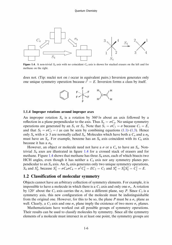
An improper rotation Sn is a rotation by 360!/n about an axis followed by areflection in a plane perpendicular to the axis. Thus Sn ¼ σCn. No unique symmetryoperations are generated by an S1 or S2. Note that S1 ¼ σC1 ¼ σ because C1 ¼ E,and that S2 ¼ σC2 ¼ i as can be seen by combining equations (1.1)–(1.3). Henceonly Sn with n ⩾ 3 are normally called Sn. Molecules which have both a Cn and a σhmust have an Sn. For example, benzene has an S6 axis coincident with its C6 axisbecause it has a σh.

However, an object or molecule need not have a σ or a Cn to have an Sn. Non-trivial S4 axes are illustrated in figure 1.4 for a crossed stack of erasers and formethane. Figure 1.4 shows that methane has three S4 axes, each of which bisects twoHCH angles, even though it has neither a C4 axis nor any symmetry planes per-pendicular to an S4 axis. An S4 axis generates only two unique symmetry operations,S4 and S3

4 , because S24 ¼ σC4σC4 ¼ σ2C2

4 ¼ EC2 ¼ C2 and S44 ¼ S2

4S24 ¼ C2

2 ¼ E.

1.2 Classification of molecular symmetryObjects cannot have an arbitrary collection of symmetry elements. For example, it isimpossible to have a molecule in which there is a C3 axis and only one σv. A rotationby 120! about the C3 axis carries the σv into a different plane, say P. Since C3 is asymmetry axis, this new configuration of the molecule must be indistinguishablefrom the original one. However, for this to be so, the plane P must be a σv plane aswell. Clearly, a C3 axis and one σv plane imply the existence of two more σv planes.

Mathematicians have worked out all possible groups of symmetry operations.Their results can be used to classify molecules by symmetry. Since all the symmetryelements of a molecule must intersect in at least one point, the symmetry groups are

C4σh

S4

1

1

2

2

3

3

4

4

S4

S4

Figure 1.4. A non-trivial S4 axis with no coincident C4 axis is shown for stacked erasers on the left and formethane on the right.

Quantum Chemistry

1-6

called point groups. Each group is designated by a symbol called the Schoenfliessymbol.

An atom has spherical symmetry and belongs to the K point group. To assign amolecule to a point group, use the flow chart given in figure 1.5. The first step is todecide whether the molecule is linear (all atoms on a straight line). If it is linear, then it

Linear? i? D∞h

C∞v

2 or more C5? i? Ih

I

2 or more C4? i? Oh

O

4 C3? σ? i? Th

T Td

Cn, n > 1? n C2 ⊥ Cn? σh? Dnh

σ? Cs σh? Cnh nσv? Dnd

i? Ci nσv? Cnv Dn

C1 S2n? S2n

Cn

Yes Yes

Yes Yes

Yes Yes

Yes Yes Yes

Yes, n ← nmax Yes Yes

Yes

Yes

Yes

Yes

Yes

Yes

No

No

No

No

No

No

No

No

No

No

No No

No

No

No

No

No

oNoN

Figure 1.5. Flow chart for determining point group symmetry.

Quantum Chemistry

1-7

has C1v orD1h symmetry depending on whether or not it has an inversion center. Forexample, carbon dioxide (O¼C¼O) has D1h symmetry but HCN has C1v symmetry.

If the molecule is not linear, then search for non-trivial axes of rotation Cn withn > 1. It helps to know that if there is a Cn axis, then all the off-axis nuclei can beseparated into sets of n equivalent nuclei. If there are multiple Cn with n > 2, thenthe molecule belongs to a high-symmetry ‘Platonic’ group. Six C5 axes indicate Ih,the point group of a perfect icosahedron or pentagonal dodecahedron, or the rare I,which has only the pure rotations of an icosahedron. Buckminsterfullerene C60 hasIh symmetry. Three C4 axes indicate Oh, the point group of a cube or a perfectoctahedron like SF6, or the rare O which has only the pure rotations of an octa-hedron. Four C3 axes and no C4 axes indicate Td, the group of a perfect tetrahedronlike methane, or the rare T which has only the rotations of Td, or Th obtained bycombining an inversion center with the rotations of T. The I, O, Th, and T pointgroups are chemically rare.

If there are no Cn axes at all with n > 1, the molecule is of low symmetry andbelongs to (a) Cs if there is a symmetry plane, (b) Ci if there is a center of inversion,and (c) C1 otherwise. If there are some Cn with n > 1, choose a principal axis with themaximum n. From this point on, n is the fixed number that you determined in thisstep. Check for nC2 axes perpendicular to the principal axis of symmetry. Next, searchfor a horizontal plane of symmetry, σh. Don’t assume that the molecular plane in aplanar molecule is a σh. For example, the molecular plane in benzene is a σh but themolecular plane in H2O is a σv. On those rare occasions when you have to look for anS2n axis, bear in mind that 2n is always even and that 2n ⩾ 4 because n > 1. Moleculeswith Dn or S2n symmetry are uncommon. For example, C(C6H5)4 has S4 symmetry,and ethane in a conformation that is neither staggered nor eclipsed has D3 symmetry.Use table 1.1 to check for all the symmetry elements characteristic of the point group.

Practice finding the point groups2 for the molecules in figure 1.6. Visualizationsoftware that allows rotation of a molecule’s ball-and-stick image in three dimen-sions is helpful. Newman projections, as taught in organic chemistry, help you seeDn, Dnd, and Dnh symmetry.

2 From left to right, first row: C1, Ci, Cs, C2; second row: C2v, C3v, C4v, C2h; third row: D2h, D3h, D6h, Oh;fourth row: D2d, D3d, Td.

Table 1.1. Characteristic symmetry elements of point groups. n ⩾ 2.

Simple Single-axis groups Dihedral groups

C1 E Cn Cn Dn Cn, nC2 ð\CnÞCs σ Cnv Cn, nσv Dnd Cn, nC2 ð\CnÞ, nσd,S2n

Ci i Cnh Cn, σh Dnh Cn, nC2 ð\CnÞ, nσv, σhInfinite groups Platonic groups

C1v C1,1σv Td 4C3, 3C2, 6σd, 3S4

D1h C1,1σv, i, σh Oh 3C4, 4C3, i, 6σd, 3σhK 1 C1 Ih 6C5, 10C3, i, 15σ

Quantum Chemistry

1-8

1.3 Implications of symmetryThe dipole moment of a molecule should not be changed either in direction or inmagnitude by a symmetry operation. This invariance to symmetry operations can berealized only if the dipole moment vector is contained in each of the symmetryelements. For example, an inversion center, more than one Cn axis, and a horizontalsymmetry plane all eliminate the possibility of a dipole moment. Therefore, amolecule can have a non-zero dipole moment only if it belongs to one of the pointgroups C1, Cs, Cn or Cnv. Thus H2O with C2v symmetry can and does have anon-zero dipole moment, but CO2 with D1h symmetry cannot and does not havea non-zero dipole moment.

A chiralmolecule is one that cannot be superimposed on its mirror image. Thus, amolecule can be chiral only if it does not have a symmetry element that converts aright-handed object to a left-handed one. In other words, a molecule can be chiralonly if it does not have a plane of symmetry or an inversion center or an improperaxis of symmetry Sn. Since S1 ¼ σ and S2 ¼ i, we can simply say that the presence ofan improper axis of symmetry rules out chirality. A molecule can be chiral only if itbelongs to a Cn or Dn point group.

In discussions of rotational spectroscopy, it is usual to classify molecules into fourkinds of rotors or tops. The correspondence between that classification and pointgroups is simple. Linear rotors are C1v or D1h molecules. Spherical tops containmore than one Cn axis with n ⩾ 3 as in Td, Oh or Ih molecules. Symmetric tops aremolecules that contain one and only one Cn axis with n ⩾ 3 or an S4 axis, and thusbelong to Cn, Cnv, Cnh, Dn, Dnh or Dnd with n ⩾ 3 or D2d or Sn ðn ¼ 4, 6, 8, . . .Þ.

CC

H

F

B

l

r

C

CH

H

B

B

l

lr

r

C

CHH

Fl

C

C

l

l

HHO

HHH

NF

F F

FF

ICC

H

H F

F

CCH H

HH

F F

F

B

F

FF

F

FF

S

C CCH

HH

H

H

H

HHH

HCH

H

H

HFigure 1.6. Molecules with various symmetries.

Quantum Chemistry

1-9

Asymmetric tops are molecules that do not contain any Cn axis with n ⩾ 3 or S4 axis,and thus belong to C1, Ci, Cs, C2, C2v, C2h, D2 or D2h.

Two symmetry operations, O1 and O2, are said to commute if the result of car-rying out one after the other does not depend upon the order in which they arecarried out. That isO1 andO2 commute ifO1O2 ¼ O2O1 whereO1O2 means first doO2 and then do O1. Symmetry operations do not always commute. For example,figure 1.7 shows that, in an equilateral triangle, reflections in the σv do not commutewith one another; in symbols, we write σ0vσv 6¼ σvσ

0v. Figure 1.7 also shows that

σ0vσv ¼ C3 and σvσ0v ¼ C2

3 .Groups in which each symmetry operation commutes with every other symmetry

operation are called Abelian. Every element of an Abelian group forms a class byitself. Note that the symmetry group of an asymmetric top molecule is always anAbelian point group. The energy levels of molecules with Abelian symmetry have aspecial simplicity as we shall see in section 4.2.

Problems (see appendix B for hints and solutions)1.1 Which of the molecules in figure 1.6 has a center of inversion?

1.2 Suppose the z axis is a C4 axis of symmetry. What will be the coordinates of anucleus after a clockwise C4 rotation if its coordinates were (x, y, z) before therotation?

σv

C3

1 2

3

σv

2 1

3

2 3

1σv σv

σv

C23 = C−1

3

1 2

3

σv

1 3

2

3 1

2σv σv

Figure 1.7. Non-commutativity of reflections in an equilateral triangle.

Quantum Chemistry

1-10

1.3 Use sketches to show all the symmetry elements in naphthalene.

1.4 Use sketches to show all the symmetry elements in the following molecules:

1.5 Find two planes of symmetry and three C2 axes in allene (C3H4).

CH

H HCC

H

Use sketches to show the symmetry elements. Drawing Newman diagrams (pro-jections) in the manner of organic chemistry books is helpful.

1.6 Find the symmetry point group for each of the following molecules. Whichmolecules are polar and which are chiral?

NH

H

H

H

HB

N

N

BN

B

H

H

H

HH

H

F

HHH Sn

Cl Cl

ClCl

1.7 Find the symmetry point group for each of the following molecules. Whichmolecules are polar and which are chiral?

C

H

H FF

1.8 A molecule has three C2 axes that are perpendicular to each other, and no othernon-trivial symmetry elements. Can such a molecule have a non-zero dipolemoment? Can it be chiral? Explain without reference to the point group of themolecule.

Quantum Chemistry

1-11

IOP Concise Physics

Quantum ChemistryA concise introduction for students of physics, chemistry, biochemistry and materials science

Ajit J Thakkar

Chapter 2

Basic quantum mechanics

2.1 Wave functions specify a system’s stateNewton’s laws do not describe correctly the behavior of electrons inmolecules; instead,quantum mechanics is required. Following early foundation work by Max Planck,Albert Einstein, Niels Bohr, and Louis de Broglie, modern quantum mechanicswas discovered in the 1920s, primarily by Werner Heisenberg, Max Born, ErwinSchrödinger, Paul Dirac, and Wolfgang Pauli. All nine won Physics Nobel Prizes.

The justification for quantum mechanics is that it provides an accurate descrip-tion of nature. As Bohr said, ‘It is wrong to think that the task of science is to findout how Nature is. Science concerns what we can say about Nature.’

In quantum mechanics, the state of a system is completely specified by a functioncalled the time-dependent state or wave function. It is a function of the time t, and ofthe three position coordinates of each of the particles in the system. A system whichis not subject to time-varying external forces can be described by a time-independentwave function ψ (read ψ as sigh), which is a function of the position coordinatesbut does not depend on the time. In this book we focus exclusively on such systems.Hence, all wave functions will be time-independent unless explicitly stated otherwise.

For example, the wave function of a one-particle system can be written as ψ(x, y, z)where (x, y, z) are the Cartesian coordinates of the position of the particle. The wavefunction contains all the information that can be known about the system. MaxBorn’s interpretation of the wave function is that jψ j2 is a probability density. Thus,for a one-particle system, the probability that the particle is in a tiny box centered at(x, y, z) with sides dx, dy, and dz is given by jψðx, y, zÞj2 dx dy dz, where dx dy dz iscalled the volume element1.

1 The probability density jψ j2 is real and non-negative, as it must be, even if the wave function ψ is complex-valued. In that case, jψ j2 ¼ ψ*ψ where the asterisk denotes complex conjugation; appendix A has a briefreview of complex numbers. In this book, we will work only with real-valued wave functions, and so jψ j2 willbe the same as ψ2.

doi:10.1088/978-1-627-05416-4ch2 2-1 ª Morgan & Claypool Publishers 2014

To ensure that the sum of the probabilities for finding the particle at all possiblelocations is finite, the wave function ψ must be square-integrable:

Rjψðx, y, zÞj2

dx dy dz<1. For example, ψ ¼ e$x2 is square-integrable over $1 ⩽ x ⩽ 1 butψ ¼ eþx2 is not.

0x

0x

e−x2

e+x2

Probabilities are usually expressed on a scale from 0 (no chance) to 1 (certainty).The certainty that the particle is somewhere leads to the normalization condition forthe wave function:

Zjψðx, y, zÞj2 dx dy dz ¼ 1: ð2:1Þ

Clearly, the wave function must be continuous for it to yield a physically sensibleprobability density. All this is summarized in:

Postulate 1. The state of a system not subject to external time-varying forces is specifiedcompletely by a continuous and square-integrable wave function ψ that depends onthe coordinates of the particles. The quantity jψ j2 dτ is the probability of finding theparticles in a volume element dτ at a given location.

2.2 Operators represent observablesIn quantum chemistry, every physical observable is represented by an operator.Hence, we first study operators and then quantum chemical ones.

2.2.1 Operators

A function of one variable, like sin(x), is a ‘black box’ that takes any real number xas input and produces a real number as output. Similarly, an operator is a black boxthat takes a function (or vector) as input and produces a function (or vector) asoutput. For example, the differentiation operator d/dx takes the function sin(x) asinput and produces the function cos(x) as output. A ‘hat’ may be used to indicatethat a symbol represents an operator; for example, A fðxÞ ¼ gðxÞ indicates that theoperator A maps the function f(x) on to the function g(x).

We have already encountered, in equations (1.1)–(1.3), the symmetry operatorsC2, σxy and i, which map a vector containing the Cartesian coordinates of a point toa vector containing the coordinates of the location to which the point is moved bythe corresponding symmetry operation. A symmetry operator can act on a functionby changing the arguments of the function. For example, the inversion operator

Quantum Chemistry

2-2

changes the sign of all the arguments of a function and this can be written asi f ðx, y, zÞ ¼ f ð$x,$y,$zÞ.

Operators work mostly as we expect. The product of a scalar (number) c andan operator A is another operator cA defined by ½cA' f ðxÞ ¼ c½Af ðxÞ'. The sum oftwo operators is defined by ½A þ B' f ðxÞ ¼ Af ðxÞ þ B f ðxÞ. The product AB of twooperators A and B is defined by AB f ðxÞ ¼ A½B f ðxÞ'. Note that the operator on theright acts first on the function and its output is acted upon by the operator onthe left. A

2is just A applied twice. In many cases, operator multiplication is non-

commutative, that is AB 6¼ BA. For example, the operator A ¼ x that multiplies afunction by x and the differentiation operator B ¼ d=dx do not commute:

AB f ðxÞ ¼ x f 0ðxÞ 6¼ BA f ðxÞ ¼ d=dx½x f ðxÞ' ¼ x f 0ðxÞ þ f ðxÞ: ð2:2Þ

Another example of operators that do not commute with each other is provided byσv and σv0 under D3h symmetry as shown in figure 1.7.

If an operator A maps a function f onto itself multiplied by a constant a, that is if

Af ðxÞ ¼ af ðxÞ, ð2:3Þ

then the function f (x) is said to be an eigenfunction of A and the constant a is calledthe corresponding eigenvalue. For example, let A ¼ d=dx and f ðxÞ ¼ 5 e3x. ThenAf ðxÞ ¼ dð5 e3xÞ=dx ¼ 15 e3x ¼ 3f ðxÞ and so 5 e3x is an eigenfunction of the dif-ferentiation operator d=dx with eigenvalue 3.

If f is an eigenfunction of A with eigenvalue a, then so is any non-zero multipleof f. To see this, note that

Aðc f Þ ¼ cðA f Þ ¼ cða f Þ ¼ aðc f Þ ð2:4Þ

in which c is a non-zero constant.An operator A is linear if, for all functions f and g, and all constants a and b, it is

true that

A a f þ b gð Þ ¼ aA f þ bA g: ð2:5Þ

Many operators, such as the differentiation operator, are linear. The square rootoperator is an example of an operator that is not linear. All quantum mechanicaloperators are linear and Hermitian. An operator A is Hermitian if

Zϕ*ðAψÞ dx ¼

Zψ*ðAϕÞ dx

! "*ð2:6Þ

is true for all functions ϕ and ψ . Hermitian operators have two important properties.(a) All the eigenvalues of a Hermitian operator are real numbers. (b) If f1ðxÞ andf2ðxÞ are any pair of distinct eigenfunctions of a Hermitian operator, then they are,or can be chosen to be, orthogonal to one another:

Z þ1

$1f1ðxÞ f2ðxÞ dx ¼ 0: ð2:7Þ

Quantum Chemistry

2-3

If the functions are complex-valued, then f1ðxÞ should be replaced by f *1 ðxÞ inequation (2.7).

2.2.2 Quantum chemical operators

Postulate 2. Every observable A is represented by a linear, Hermitian operator A. Theoperator x for each coordinate x corresponds to multiplication by x, and the operator foreach component of linear momentum px is px ¼ $iħ@=@x (read ħ as h-bar) in whichħ ¼ h=2π and h is Planck’s constant. All other operators are constructed by replacingCartesian coordinates and linear momenta in the Newtonian formula for A by these two.

Postulate 3. The only values that can be observed in a measurement of an observableA are the eigenvalues of the corresponding operator A.

The eigenvalues of postulate 3 are guaranteed to be real numbers, as they must beif they are to be the results of observations, because the operators are Hermitian.The px operator would not be Hermitian without the constant i ¼

ffiffiffiffiffiffiffi$1

p. Often the

hat ^ is left off x and other multiplicative operators. Observe that equation (2.2)shows that x does not commute with px.

All other quantum chemical operators are constructed from the position andmomentum operators. For example, the operator T x for the x component of thekinetic energy of a particle of mass m is obtained as follows:

Tx ¼p2x2m

¼ ð$iħÞ2

2m@

@x

$ %2¼ $ ħ2

2m@2

@x2: ð2:8Þ

The total kinetic energy operator for a single particle of mass m is

T ¼ Tx þ T y þ T z ¼ $ ħ2

2mr2 ð2:9Þ

in which

r2 ( @2

@x2þ @2

@y2þ @2

@z2

is called the Laplacian operator or ‘del-squared’. Sometimes r2 is denoted by Δ(read Δ as dell-tah). The potential energy V depends only on the coordinates andso V for a single particle is simply multiplication by the potential energy functionVðx, y, zÞ. The total energy operator is called the Hamiltonian operator:

H ¼ T þ V : ð2:10Þ

The hat is usually left off V because it is a multiplicative operator. Insertingequation (2.9) into equation (2.10), we get the single-particle Hamiltonian

H ¼ $ ħ2

2mr2 þ V x, y, zð Þ: ð2:11Þ

Quantum Chemistry

2-4

Hamiltonians for systems with more than one particle are discussed in section 6.2.The next section explains the fundamental role of the Hamiltonian operator.

2.3 Schrödinger’s equationPostulate 4. The wave functions ψ of a system free of time-varying external forces areeigenfunctions of the Hamiltonian operator H :

Hψ ¼ Eψ : ð2:12Þ

Postulate 3 tells us that the observable energies are eigenvalues of the energy(Hamiltonian) operator. Postulate 4 tells us that the eigenfunctions of the Hamil-tonian are precisely the wave functions of postulate 1.

Equation (2.12) is called the Schrödinger equation. Since it has many solutions,equation (2.12) is often written as

Hψn ¼ Enψn ð2:13Þ

where the quantum number n ¼ 1, 2, . . . labels the states in order of increasing energy.Since H is Hermitian, the energy eigenvalues En are real numbers as they must beand the eigenfunctions ψn are orthogonal to one another (see equation (2.7)):

Zψmψn dτ ¼ 0 for m 6¼ n: ð2:14Þ

The normalization and orthogonality conditions, equation (2.1) and equation (2.14),can be combined in the compact orthonormality condition:

Zψmψn dτ ¼

1 for m ¼ n,0 for m 6¼ n

&ð2:15Þ

in which dτ is the pertinent volume element; for example, dτ ¼ dx dy dz for a singleparticle. If the wave functions are complex-valued, then ψm should be replaced byψ*m in equations (2.14)–(2.15).Equation (2.4) tells us that if ψ 0 is an eigenfunction of H with energy E, then so is

ψ ¼ cψ 0 where c is any non-zero constant. We exploit this to choose c in a mannersuch that ψ is normalized. We require

Zjψ j2 dτ ¼

Zjc ψ 0j2 dτ ¼ jcj2

Zjψ 0j2 dτ ¼ 1:

If c is a real number, then

c ¼ )Z

jψ 0j2 dτ$ %$1=2

ð2:16Þ

and we can choose either the positive or the negative sign because both choices leadto the same probability density jψ j2. This is referred to as the choice of the phasefactor. Usually the positive sign is chosen for simplicity.

Quantum Chemistry

2-5

For example, suppose that ψ 0 ¼ e$bx2 is an unnormalized wave function for asingle particle in one dimension and that the range of x is ð$1,1Þ. Insert ψ 0 ¼ e$bx2

into the integral in equation (2.16), note that b > 0 is required for square integra-bility, and use the integral formula (A.15) on page A-3, to find that

Zjψ 0j2 dτ ¼

Z 1

$1e$2bx2 dx ¼ π

2b

' (1=2:

Choosing the positive root leads to the normalization constant c ¼ ð2b=πÞ1=4 and thenormalized wave function ψ ¼ ð2b=πÞ1=4 e$bx2 .

2.4 Measured and average valuesA way to compute the average value of an observable A that we can expect to obtainin a series of measurements on a set of identical systems is given by the next postulate.

Postulate 5. If a system is in a state described by a normalized wave function ψ , thenthe average value of the observable A with corresponding operator A is given by

hAi ¼Z

ψðAψÞ dτ: ð2:17Þ

Equation (2.17) must be written as hAi ¼Rψ*ðAψÞ dτ if the wave function is

complex-valued. An average need not coincide with any of the numbers it is con-structed from. Hence the expectation (or average) value hAi need not coincide withany of the eigenvalues of A. The variance of the values of A found by measurementson a set of identical systems is given by

σðAÞ ¼'hA2i$ hAi2

(1=2: ð2:18Þ

The Heisenberg uncertainty principle is:

σðxÞσðpxÞ⩾ħ=2: ð2:19Þ

Heisenberg’s inequality implies that σ(x) and σ( px) cannot both be zero althoughone can be zero if the other is infinite. In other words, we cannot simultaneouslymeasure the position and momentum of a particle without introducing an inherentuncertainty in one or both of these quantities. Similar Heisenberg inequalities holdfor the y and z components2.

2Moreover, Howard P Robertson showed that uncertainty relationships hold true for all pairs of operators,ðA, BÞ, that do not commute with each other:

σ Að Þσ Bð Þ⩾ 1

2hjAB $ BAji: ð2:20Þ

Inserting the quantum mechanical operators for x and px into equation (2.20) and doing some algebra (seeequation (2.2)) leads to the Heisenberg uncertainty principle given by equation (2.19).

Quantum Chemistry

2-6

If quantum mechanics makes you uneasy, pay heed to Richard Feynman (NobelPrize, 1965). He said, ‘Do not keep saying to yourself: “But how can it be like that?”because you will go down the drain into a blind alley from which nobody has yetescaped. Nobody knows how it can be like that. But all known experiments back upquantum mechanics.’

Problems (see appendix B for hints and solutions)2.1 Evaluate g ¼ Af for (a) A ¼ d2=dx2 and f ðxÞ ¼ e$ax, (b) A ¼

R a0 dx and

f ðxÞ ¼ x3 $ 2x2 þ 3x$ 4, and (c) A ¼ r2 and f ðx, y, zÞ ¼ x4y3z2.

2.2 Write down the form of the operator A2when (a) A ¼ x, (b) A ¼ d=dx, and

(c) A ¼ d=dxþ x. Make sure you include a function f before carrying out operationsto check your answer.

2.3 Which of the following functions (a) e$αx2 , (b) cos βx, and (c) 7eikx are eigen-functions of the operator $ħ2d2=dx2? For each eigenfunction, what is thecorresponding eigenvalue?

2.4 Are the functions f ðxÞ ¼ e$3x2 and gðxÞ ¼ eþ3x2 square integrable over$1 < x < 1? Would the answer change if the constant 3 in these functions waschanged to 5 or 99?

2.5 Jan and Olga were working on solutions to the Schrödinger equation for amodel one-dimensional problem. They squabbled because Jan found the ground

state wave function to be ψ ¼ ζ3=2π) *1=2

e$ajxj whereas Olga found it to be

ψ ¼ $ ζ3=2π) *1=2

e$ajxj where a and ζ are constants. Their director, Susan, explainedto them why they were both right. What was Susan’s explanation?

2.6 Write down the three mathematical statements implied by ‘the real-valuedfunctions f(x) and g(x) are orthonormal on the interval [0, 1)’.

2.7 Suppose ψ 0 ¼ e$ar is an unnormalized wave function for a single-particle,one-dimensional system. The range of r is (0,1), and a > 0 as is required for squareintegrability. Find c such that ψ ¼ cψ 0 is normalized.

Quantum Chemistry

2-7

IOP Concise Physics

Quantum ChemistryA concise introduction for students of physics, chemistry, biochemistry and materials science

Ajit J Thakkar

Chapter 3

Translation and vibration

3.1 A particle in a wireThe postulates of quantum mechanics can be understood by considering a simpleone-dimensional model of the translational motion of a particle in a wire. Many ofthe features encountered here, including quantization of energy levels, orthogonalityof wave functions, increase in energy with number of nodes in the wave function,and symmetry of wave functions, recur throughout this book.

Consider a particle of mass m that can move freely along a straight piece of wireof length a but is prevented from leaving the wire by infinitely high walls as infigure 3.1. This model of translational motion is used in statistical thermodynamicswhen the macroscopic properties of an ideal gas are related to the properties of themolecules comprising the gas.

The potential energy is zero inside the wire and at its ends, but infinite elsewhereso that the particle cannot leave the wire. Let the wire be placed along the x axis andextend from x ¼ 0 to x ¼ a. Since the particle will be restricted to the x axis, this isa one-dimensional problem. ψ(x) ¼ 0 for x < 0 and x > a because the probability of

V = ∞

ψ = 0

0

V = 0

ψ = ?

a

V = ∞

ψ = 0

xFigure 3.1. A particle in a wire.

doi:10.1088/978-1-627-05416-4ch3 3-1 ª Morgan & Claypool Publishers 2014

the particle being outside the wire is zero. To find ψ in the wire, we must solve theSchrödinger equation (2.12) using a one-particle Hamiltonian, equation (2.11),with V ¼ 0 and the kinetic energy operator containing only an x component. Thus,we must solve:

" ħ2

2md2ψdx2

¼ Eψ for 0⩽ x⩽ a: ð3:1Þ

3.1.1 Solving the Schrödinger equation

Equation (3.1) is solved by noticing that the only functions whose second derivativesare proportional to themselves, with a negative proportionality constant, are the sineand cosine functions. So we try the function:

ψðxÞ ¼ A sin αxþ B cos βx for 0⩽ x⩽ a: ð3:2Þ

Postulate 1 on page 2-2 says that ψ must be continuous everywhere. Continuity atthe left edge (x ¼ 0) requires ψð0Þ ¼ 0 which forces A× sin 0þ B× cos 0 ¼ B ¼ 0.Hence equation (3.2) reduces to ψðxÞ ¼ A sin αx in the wire. Next, continuity atx ¼ a requires ψðaÞ ¼ A sin αa ¼ 0 and hence αa ¼ &nπ or A ¼ 0 where n is aninteger. The wave function cannot be zero everywhere inside the wire and so A ¼ 0and n ¼ 0 are not physically admissible. This means that ψnðxÞ ¼ A sinðnπx=aÞ withn 6¼ 0. Changing the sign of n merely changes the sign and phase factor of ψ . Hence,the negative values of n do not lead to solutions that are physically distinct fromthose with positive n (see section 2.3), and it is sufficient to consider only positive n.The constant A can be found from the normalization condition (2.1). Using theintegral in equation (A.9) from appendix A, we get:

Z a

0jψn xð Þj2 dx ¼ jAj2

Z a

0sin2 nπx=að Þ dx ¼ jAj2a

2¼ 1: ð3:3Þ

Hence jAj ¼ffiffiffiffiffiffiffiffi2=a

pand we can choose A ¼

ffiffiffiffiffiffiffiffi2=a

p. Finally, substitute ψnðxÞ ¼

A sinðnπx=aÞ into the Schrödinger equation (3.1), and find

" ħ2

2md2ψn

dx2¼ ħ2n2π2

2ma2ψn ¼

h2n2

8ma2ψn ¼ Enψn: ð3:4Þ

In summary, we have found the wave functions

ψnðxÞ ¼2=að Þ1=2 sin nπx=að Þ inside the wire: 0⩽ x⩽ a

0 outside the wire: x< 0, x> a

(

ð3:5Þ

Quantum Chemistry

3-2

for n ¼ 1, 2, . . ., and from equation (3.4), the corresponding energies

En ¼h2n2

8ma2for n ¼ 1, 2, . . .: ð3:6Þ

The quantum number n ¼1, 2, . . . labels the wave functions and energies.

3.1.2 The energies are quantized

Equation (3.6) and figure 3.2 show that only certain energies are allowed; we say thatthe energies are quantized. The lowest energy state (n ¼ 1 in this case) is called theground state, and the higher energy states (n> 1 in this case) are called excited states.

The lowest allowable energy is called the zero-point energy and is greater thanzero in this problem. It implies that a quantum particle in a wire is always movingaround! In this model, the Heisenberg uncertainty principle makes E1 ¼ 0 impos-sible because it would imply hp2xi ¼ hpxi ¼ σðpxÞ ¼ 0 since all the energy is kinetic.That in turn would require σðxÞ to be infinite to satisfy the Heisenberg principle.However, σðxÞ cannot be infinite because the particle is confined to a wire offinite length.

The spacing between adjacent energy levels, Enþ1 " En, increases as n increases.As the wire gets longer (a increases) or the particle gets heavier (m increases), thespacings Enþ1 " En get smaller and the energy levels are squished closer together.There is almost a classical energy continuum for heavy enough particles and longenough wires. The largest quantum effects are seen for extremely light particles invery short wires.

Einstein’s relationship E ¼ hν gives ν ¼ ðEu " ElÞ=h as the frequency (read ν asnew) of a photon that can excite the particle from state l to u and of a photon emittedwhen a particle relaxes from state u to l; see problem 3.2.

νu

l

0

8ma2

h2 E

1

4

9

16

E1

E2

E3

E4

Figure 3.2. Energy levels of a particle in a wire, En ¼ h2n2=ð8ma2Þ.

Quantum Chemistry

3-3

3.1.3 Understanding and using the wave functions

The wave functions of equation (3.5) and their squares are shown in figure 3.3. Theprobability of finding the particle is not the same at all locations in the wire; seeproblem 3.4. The probability density oscillates in the excited states. In the limit asn ! 1, the peaks of the oscillations are so close together that the probability densityis essentially uniform inside the wire. The points inside the wire at which the wavefunctions cross the x axis and become zero are called nodes or zero crossings. Theenergy of a state increases with the number of nodes in the corresponding wave function.

There is a center of inversion at the midpoint of the wire, x ¼ a=2. The inversionoperator i interchanges the points a=2þ E and a=2" E (read E as ep-si-lawn) which isequivalent to the interchange of x and a" x. The wave functions for the states withodd n are symmetric under inversion—that is i ψnðxÞ ¼ ψnðxÞ for n ¼ 1, 3, 5, . . .. Thewave functions for the even n states are antisymmetric under inversion, that isi ψnðxÞ ¼ "ψnðxÞ for n ¼ 2, 4, 6, . . .. The probability densities jψnðxÞj

2 are sym-metric under inversion for all n as they must be since the two halves of the wire arephysically indistinguishable. Hence, the probability of finding the particle in eitherhalf of the wire is

R a=20 ψnj j2 dx ¼

R aa=2 ψnj j2 dx ¼ 1=2. The wave functions ψnðxÞ are

eigenfunctions of a Hermitian operator and hence orthogonal to one another (seeequation (2.14)):

Z a

0ψnðxÞψmðxÞ dx ¼ 0 for n 6¼ m: ð3:7Þ

xx

n = 1

n = 2

n = 3

n = 4

00 aa

ψn(x) |ψn(x)|2

Figure 3.3. Wave functions ψnðxÞ and probability densities jψnðxÞj2 for the four lowest states of a particle in

a wire.

Quantum Chemistry

3-4

Average values of observables can be calculated from the wave functions usingpostulate 5. For example, using the ground-state wave function ψ1ðxÞ from equation(3.5), the x operator from postulate 2, equation (2.17), and the formula of equation(A.10) from appendix A to do the final integral, we find that the average value of theposition of a particle in a wire in its ground state is:

hxi ¼Z

ψ1 xψ1ð Þ dτ ¼ 2

a

Z a

0sin πx=að Þx sin πx=að Þ dx ¼ a=2:

The result makes sense because the probability density is symmetric with respect tothe center of the wire.

3.2 A harmonic oscillatorA harmonic oscillator is a one-dimensional model for vibrational motion. Visualizeit as a ball attached to a rigid surface by an ideal spring. A particle of mass mundergoing harmonic motion in the x direction experiences a restoring force pro-portional to its displacement. We choose x ¼ 0 to be the equilibrium point of zerodisplacement; positive values of x correspond to stretching and negative values tocompression of the spring. Then F ¼ "kx in which the force constant k> 0 is ameasure of the spring’s stiffness. Since F ¼ "dV=dx, the potential is V ¼ kx2=2, andthe Schrödinger equation is

" ħ2

2md2ψdx2

þ 1

2kx2ψ ¼ Eψ : ð3:8Þ

x

V

The allowed energy levels are found, by an involved derivation, to be

Ev ¼ ħωðvþ 1=2Þ for v ¼ 0, 1, 2, . . . ð3:9Þ

in which ω ¼ k=mð Þ1=2 is the vibrational frequency (read ω as o-may-gah), and vis the quantum number. The zero-point (ground v ¼ 0 state) vibrational energyis E0 ¼ ħω=2; a quantum oscillator never stops vibrating. The energy level spacing isconstant: Evþ1 " Ev ¼ ħω; see figure 3.4. The spacing ħω and zero-point energy E0

increase as the particle mass m decreases and the force constant k increases. Lighterparticles and stiffer springs vibrate faster.

Examination of figure 3.5 reveals that ψ vðxÞ has v nodes. As it does for a particlein a wire, the energy of a state increases as the number of nodes in the wave functionincreases. The wave functions are eigenfunctions of the inversion operator i thatchanges the sign of x. The even v states are symmetric and the odd v states are

Quantum Chemistry

3-5

antisymmetric with respect to i; that is, i ψ vðxÞ ¼ ψ vðxÞ for v ¼ 0, 2, 4, . . . andi ψvðxÞ ¼ "ψ vðxÞ for v ¼ 1, 3, 5, . . ..

In Newtonian mechanics, an oscillator reaches its points of greatest displacement,called classical turning points, when all its energy is potential energy. Figure 3.5shows that as v becomes large, the probability density peaks near the classicalturning points. Observe in figure 3.5 that there is a non-zero probability of dis-placements that lie outside the classically allowed region from x ¼ "

ffiffiffiffiffiffiffiffiffiffiffiffiffiffiffiffiffiffiffiffiffiffið2vþ 1Þ=α

pto

x ¼ þffiffiffiffiffiffiffiffiffiffiffiffiffiffiffiffiffiffiffiffiffiffið2vþ 1Þ=α

p. This feature, called tunneling, is characteristic of quantum

systems. Tunneling was discovered by Friedrich Hund in the wave functions for adouble-well problem and first used by George Gamow to explain features of alphadecay. Quantum mechanical tunneling is important in many different phenomena,and is exploited in scanning tunneling microscopes invented by Gerd Binnig andHeinrich Rohrer (Physics Nobel Prize, 1986).

xx

v = 0

v = 1

v = 2

v = 3

ψv(x) |ψv(x)|2

Figure 3.5. Wave functions ψ vðxÞ and probability densities jψ vðxÞj2 for the four lowest states of a harmonic

oscillator.

01/2

3/2

5/2

7/2

E

ω

E0

E1

E2

E3

Figure 3.4. Energy levels of a harmonic oscillator.

Quantum Chemistry

3-6

The wave functions for 0⩽ v⩽ 3 are listed in table 3.1. The general form of theharmonic oscillator wave functions is

ψ vðxÞ ¼ NvHvðα1=2xÞ e"α x 2=2 ð3:10Þ

where α ¼ ðkmÞ1=2=ħ ¼ mω=ħ and Nv is a normalization constant that can bedetermined using equation (2.1). The Hermite polynomial HvðyÞ ¼ a0 þ a1yþa2y2 þ ' ' ' þ avyv in which y ¼

ffiffiffiα

px and the ai are constants. The wave functions are

eigenfunctions of a Hermitian operator and hence form an orthonormal set:

Z 1

"1ψ vðxÞψ v0ðxÞ dx ¼

1 for v ¼ v 0

0 for v 6¼ v 0:

"ð3:11Þ

Average values can be calculated using equation (2.17), wave functions fromtable 3.1, and integral formulas from appendix A. For example, the average value ofx2 in the ground state is:

hx2i ¼Z 1

"1ψ0ðxÞ½x2 ψ0ðxÞ) dx

¼#απ

$1=2 Z 1

"1e"α x 2=2 x2 e"α x 2=2 dx ¼ 1= 2αð Þ:

The probability of non-classical displacements can be calculated to be 0.16 in theground state. This probability decreases as v increases.

3.2.1 Molecular vibrations

Molecular vibrations are described by the harmonic oscillator model. A diatomicmolecule is modeled as two atoms attached to each other by an ideal spring. Thepotential energy depends only on the position of one atom relative to that of theother. A center-of-mass transformation allows one to separate external from internalcoordinates in the two-particle Schrödinger equation. Only the internal vibrationalmotion is of interest, since the external motion is simply the translational motion ofthe molecule as a whole. The Schrödinger equation for the vibrational motion differsfrom the Schrödinger equation for the harmonic oscillator only in the replacementof the mass m by the reduced mass μ ¼ m1m2=ðm1 þm2Þ (read μ as mew) of themolecule where m1 and m2 are the masses of the two atoms. Hence, the harmonic

Table 3.1. Harmonic oscillator wave functions with α ¼ mω=ħ.

ψ0ðxÞ ¼ α=πð Þ1=4 e"α x 2=2

ψ1ðxÞ ¼ 4α3=πð Þ1=4 x e"α x 2=2

ψ2ðxÞ ¼ α=4πð Þ1=4 ð2α x2 " 1Þ e"α x 2=2

ψ3ðxÞ ¼ α3=9πð Þ1=4 ð2α x3 " 3xÞ e"α x 2=2

Quantum Chemistry

3-7

oscillator wave functions and energy levels, with m replaced by μ, describe thestretching vibration of a diatomic molecule.

It requires 3N coordinates to specify the positions of the atoms in a molecule withN atoms. Three coordinates are used to specify the location of its center of mass or,in other words, to describe the translational motion of the molecule as a whole. Thedisplacements of the remaining 3N " 3 coordinates (called the remaining 3N " 3degrees of freedom) describe the internal motions of the molecule. A non-linearmolecule has three independent rotations, one about each of the three axes in acoordinate system fixed at its center of mass. However, a linear molecule has onlytwo distinct rotations, one about each of the two axes perpendicular to the molecular(z) axis. One may also think of the number of independent rotations as the numberof angles needed to describe the orientation of the molecule relative to the coordinatesystem at its center of mass. All the remaining degrees of freedom describe molecularvibrations. Therefore, a molecule has 3N " 6 distinct vibrations if it is non-linear or3N " 5 if it is linear. Each vibration can be modeled as a harmonic oscillator withdifferent parameters.

Infrared and other types of spectroscopy enable us to measure the frequencies oftransitions between vibrational energy levels of a molecule. The measured frequencycan be used to deduce the force constant using the harmonic oscillator model. Thefrequency ν is related to the wavelength λ by ν ¼ c=λ, where c is the speed of light.Moreover, ν is related to the energy-level spacing by hν ¼ ΔE. The harmonicoscillator model predicts ΔE ¼ ħω. Combining these relationships gives usω ¼ 2πν ¼ 2πc=λ. Since ω ¼ ðk=μÞ1=2, it follows that k ¼ 4π2c2μ=λ2. For example,the ‘fundamental’ v ¼ 0 ! 1 vibrational transition in 35Cl2 was observed at565 cm"1; that is, 1=λ ¼ 565 cm"1. The atomic mass of 35Cl is 34.969 u and soμ ¼ 17:4845 u for 35Cl2. Converting all quantities to SI units and substituting intok ¼ 4π2c2μ=λ2 gives k ¼ 329 N m"1. Force constants for a wide variety of molecularvibrations have been obtained in this manner. Force constants give us an indicationof the relative stiffness of bonds.

Problems (see appendix B for hints and solutions)3.1 What would happen to the energy level spacing of a particle in a wire if its masswas halved?

3.2 Calculate the wavelength of the photon emitted when an electron in a wire oflength 500 pm drops from the n ¼ 2 level to the n ¼ 1 level.

3.3 Consider a particle in a wire. For which states (values of n) are the probabilitiesof finding the particle in the four quarters of the wire (0⩽ x⩽ a=4, a=4⩽ x⩽ a=2,a=2⩽ x⩽ 3a=4, and 3a=4⩽ x⩽ a) all equal to 1=4? Explain your reasoning withsketches of pertinent jψnðxÞj

2.

3.4 Consider the ground state of a particle in a wire. Calculate the probability offinding the particle in (a) the left half of the wire, and (b) in each quarter of the wire.

Quantum Chemistry

3-8

3.5 Calculate the ground-state expectation values hxi, hx2i, hpxi, and hp2xi for aparticle in a wire. Explain how the result for hp2xi makes physical sense. Then cal-culate σðxÞσðpxÞ and check whether the Heisenberg uncertainty principle is satisfiedfor the ground state of a particle in a wire.

3.6(a) The particle in a wire can be used as a very simple model of the π electrons in

1,3-butadiene. Assume that there can be no more than two electrons per energylevel on the basis of the Pauli principle that you learned in your generalchemistry course. Choose m and a in a meaningful manner. Then write down aformula for the wavelength of a photon that has precisely the energy required toinduce the promotion of an electron from the highest filled to the lowest unfilledenergy level. Finally, find a numerical value for this wavelength.

(b) Solve the same problem for 1,3,5-hexatriene.(c) Generalize the solution to conjugated polyenes with 2N carbon atoms.

3.7 What would happen to the energy level spacing of a harmonic oscillator if itsforce constant was multiplied by four?

3.8 Calculate the ground-state expectation values hxi and hx2i for a one-dimensional harmonic oscillator. Then calculate σðxÞ.

3.9 An experimental measurement of the v ¼ 0 ! 1 vibrational transition enablesus to calculate the force constant. Vibrational transitions are usually given in wavenumbers (reciprocal wavelengths): ν=c ¼ 1=λ. The wave numbers for 1H35Cl, 1H81Br,and 1H127I were found to be 2988.9, 2649.7, and 2309:5 cm"1, respectively. Theatomic masses for 1H, 35Cl, 81Br, and 127I are 1.0078, 34.969, 80.916, and 126.90 u,respectively. Use the harmonic oscillator model of molecular vibrations to calculatethe force constants in N m"1 (equivalent to J m"2) and discuss the relative stiffness ofthe bonds.

Quantum Chemistry

3-9

IOP Concise Physics

Quantum ChemistryA concise introduction for students of physics, chemistry, biochemistry and materials science

Ajit J Thakkar

Chapter 4

Symmetry and degeneracy

4.1 A particle in a rectangular plateWe noted the link between molecular symmetry and polarity in section 1.3. We sawsymmetry in the wave functions for the model systems discussed in chapter 3. Here,we study translational motion in two dimensions as a prelude to a systematicinvestigation of how symmetry affects energy levels in section 4.2, probabilitydensities in section 4.3, and wave functions in section 4.4 and section 4.5.

Consider a particle of mass m allowed to move freely within a rectangularplate, 0⩽ x⩽ a, 0⩽ y⩽ b, but trapped in it by an infinite potential energy outside theplate as shown in figure 4.1.

The wave function ψ ¼ 0 everywhere outside the plate. Within the plate, V ¼ 0and ψ is determined by the two-dimensional Schrödinger equation:

" ħ2

2m

@2ψnx,ny

@x2" ħ2

2m

@2ψnx,ny

@y2¼ Enx,nyψnx,ny : ð4:1Þ

The two-dimensional problem requires two quantum numbers.

0 a

b

V = 0 V = ∞V = ∞

V = ∞

V = ∞ x

y

Figure 4.1. A particle in a rectangular plate.

doi:10.1088/978-1-627-05416-4ch4 4-1 ª Morgan & Claypool Publishers 2014

A partial differential equation like equation (4.1) is often difficult to solve.However, in this case the technique of separation of variables can be used. Supposethat the Hamiltonian for a two-dimensional problem is the sum of two one-dimensional Hamiltonians H ¼ H x þ H y which act only on x and y, respectively,and that their eigenvalues and eigenfunctions are known:

HxφjðxÞ ¼ ɛjφjðxÞ for j ¼ 1, 2, . . . ð4:2Þ

HyϕkðyÞ ¼ EkϕkðyÞ for k ¼ 1, 2, . . .: ð4:3ÞThen the eigenfunctions of the two-dimensional Schrödinger equation

Hψ j,kðx, yÞ ¼ Ej,kψ j,kðx, yÞ ð4:4Þare given by ψ j,kðx, yÞ ¼ φjðxÞϕkðyÞ and the corresponding eigenvalues areEj,k ¼ ɛj þ Ek.

The Hamiltonian for a particle in a rectangle is separable into two one-dimensional Hamiltonians both corresponding to a particle in a wire, see section 3.1.Hence, the energies for the particle in a rectangle are

Enx,ny ¼h2

8mn2xa2

þn2yb2

!

for nx ¼ 1, 2, . . . and ny ¼ 1, 2, . . . ð4:5Þ

and the corresponding wave functions are

ψnx,nyðx, yÞ ¼4=abð Þ1=2 sin nxπx=að Þ sin nyπy=b

! "inside the plate,

0 outside the plate:

(

ð4:6Þ

Examine the wave functions shown in figure 4.2 for the four lowest-energy states.Observe that the ground-state wave function ψ1,1 does not cross zero inside the plate;that is, ψ1,1 has no interior nodes. However, the excited state wave functions are zeroat every point along certain lines, called nodal lines, inside the plate. Notice fromfigure 4.2 that ψ2,1 has a nodal line along x ¼ a=2, that ψ1,2 has a nodal line alongy ¼ b=2, and that ψ2,2 has two nodal lines, one along x ¼ a=2 and the other alongy ¼ b=2. The energy increases with the number of nodal lines but states, like ψ1,2 andψ2,1, with the same number of nodal lines may have different energies.

4.2 Symmetry leads to degeneracyConsider the effect of introducing symmetry in the two-dimensional rectangularplate of section 4.1. For example, suppose the plate is square so that b ¼ a; then theenergies of equation (4.5) simplify to

Enx,ny ¼h2

8ma2!n2x þ n2y

": ð4:7Þ

0 a

a

x

y

Quantum Chemistry

4-2

The two lowest excited state energies are equal:

E2,1 ¼ E1,2 ¼ 5h2=ð8ma2Þ ð4:8Þ

although the corresponding wave functions are different. Each different wavefunction corresponds to a different state but more than one state may have the sameenergy (or energy level). An energy level that corresponds to more than one state iscalled degenerate, with a degeneracy equal to the number of corresponding states.Thus the second lowest energy level of a particle in a square two-dimensional plate,E ¼ 5h2=ð8ma2Þ, is two-fold degenerate, whereas the ground state has a degeneracyof one and is said to be non-degenerate. Many two-fold degeneracies arise for theparticle in a square plate because En,k ¼ Ek,n for all k 6¼ n. Indeed, a particle in asquare plate has more degenerate energy levels than non-degenerate ones, as seenclearly in figure 4.3.

Degeneracies almost always arise from some symmetry of the system. For example,a particle in a square plate has C4v symmetry, and one finds symmetry-induceddegeneracies in the energy levels. The allowed degeneracies for all the point groupsare listed in table 4.1. There are no degeneracies induced by the geometrical sym-metry if the point group is Abelian (see section 1.3). A Cn axis with n ⩾ 3 is usually agood indicator of degeneracy with exceptions only for the rarely encountered Cn andCnh groups.

00

00

00

00

aa

aa

bb

bb

xx

xx

yy

yy

ψ1,1 ψ2,1

ψ1,2 ψ2,2

Figure 4.2. Wave functions for a particle in a rectangular plate.

Quantum Chemistry

4-3

Sometimes there are accidental degeneracies. For example, consider the energiesof a particle in a square, equation (4.7). When ðnx, nyÞ differs from ðnx, nyÞ by morethan an interchange, we expect n2x þ n2y 6¼ n2x þ n2y and hence Enx,ny 6¼ Enx,ny . How-ever, there are some rare cases where equality holds. For example, 52 þ 52 ¼ 12 þ 72

leads to the accidental degeneracy E5,5 ¼ E1,7 and 12 þ 82 ¼ 42 þ 72 leads toE1,8 ¼ E4,7.

There can also be degeneracies induced by a non-geometrical symmetry; forexample, such degeneracies arise in the hydrogen atom, as will be seen in section 6.3.Understanding non-geometrical symmetry is beyond the scope of this book.

4.3 Probabilities in degenerate statesHow do degenerate states differ from one another? Consider the wave functions fora particle in a square plate. Setting b ¼ a in equation (4.6) gives:

ψnx,ny x, yð Þ ¼ 2

a

# $sin

nxπxa

% &sin

nyπya

% &: ð4:9Þ

8ma2

h2 E

0

2

5

8

10

13

17

E1, 1

E2, 1,E 1, 2

E2, 2

E3, 1,E 1, 3

E3, 2,E 2, 3

E4, 1,E 1, 4

E3, 3

Figure 4.3. Energy levels of a particle in a square two-dimensional plate.

Table 4.1. Permissible degeneracies.

Group Maximum degeneracy

C1, Ci, Cs, C2v, D2, D2h, and Cn, Cnh, S2n for n ¼ 2, 3, . . . 1D2d, and Cnv, Dn, Dnd, Dnh for n ¼ 3, 4, . . . 2T, Th, Td, O, Oh 3I, Ih 5K (sphere) 1

Quantum Chemistry

4-4

The wave function for the 2,1 state equals zero along the line x ¼ a/2, whereas thewave function for the 1,2 state equals zero along the line y ¼ a/2 as indicated infigure 4.4.

The two states are related by a rotation of 90& about the C4 axis of symmetrypassing through the center of the square, ða=2, a=2Þ, and perpendicular to it; seefigure 4.2 and figure 4.4. The 90& rotation should leave the system in a configurationthat is indistinguishable from the first. Hence, the two states should have the sameenergy and they do. However, neither jψ1,2j

2 nor jψ2,1j2 can be a valid probability

density because the two are related by a C4 rotation whereas the probability densityis an observable quantity and should not change when a symmetry operation iscarried out. The solution is to notice that when there is a degeneracy, the system isequally likely to be found in any one of the degenerate states, and hence theobservable probability density is the ensemble-average of the probability densities ofthe degenerate states. Thus, the observable probability density for the two-folddegenerate ψ1,2 and ψ2,1 states is (read ρ as row):

ρ x, yð Þ ¼ 1

2

!jψ1,2j

2 þ jψ2,1j2": ð4:10Þ

Figure 4.5 shows that ρðx, yÞ is invariant to a C4 rotation and has C4v symmetryas it should. There is a node at the center of the square, four equivalent maxima at

a0 x

y

a

+ −

a0 x

y

a

+

−

Figure 4.4. Sign patterns and nodal lines of ψ2,1 (left) and ψ1,2 (right).

0

0

a

ax

y

ρ(x, y)

Figure 4.5. The ensemble-averaged probability density for the two-fold degenerate ψ1,2 and ψ2,1 states.

Quantum Chemistry

4-5

ð0:3, 0:3Þ, ð0:3, 0:7Þ, ð0:7, 0:7Þ, and ð0:7, 0:3Þ that are related by C4 rotations, andfour equivalent saddle points at ða=2, 0:3Þ, ða=2, 0:7Þ, ð0:7, a=2Þ, and ð0:3, a=2Þ thatare related by C4 rotations.

4.4 Are degenerate wave functions unique?Suppose that ψ and φ (read φ as fye) are a pair of degenerate eigenfunctions of theHamiltonian H so that Hψ ¼ Eψ and Hφ ¼ Eφ. Then any linear combination(mixture) of ψ and φ, such as f ¼ aψ þ bφ where the constants a and b are mixingcoefficients, is also an eigenfunction of H with the same energy E. This follows fromthe linearity of H (see equation (2.5)):

H f ¼ H ðaψ þ bφÞ ¼ aHψ þ bHφ ¼ aEψ þ bEφ

¼ Eðaψ þ bφÞ ¼ Ef : ð4:11Þ

In other words, degenerate wave functions are not unique.A pair of doubly degenerate wave functions (ψ , φ) can be replaced by a different

pair of functions, f as defined above and g ¼ cψ þ dφ, provided that we take care tochoose the mixing coefficients, a, b, c, and d, such that f is normalized, g is nor-malized, and that f and g are orthogonal to each other. One degree of freedom is leftafter these three requirements on four constants are satisfied. The requirements aremet by choosing a ¼ d ¼ cosΩ and b ¼ "c ¼ sinΩ—that is, by requiring thetransformation to be unitary. Note that Ω ¼ 0& leads to no change at all (f ¼ ψ ,g ¼ φ), and that Ω ¼ 90& leads to (f ¼ φ, g ¼ "ψ), which amounts to no more thanchanging the sign of one of the functions. This transformation of degenerate wavefunctions is akin to rotating the axes of a coordinate system by an angle Ω whilepreserving the orthogonality and normalization of the basis vectors. Both pairs ofcoordinate axes in figure 4.6 are equally valid but one set may be more useful thanthe other in a particular problem. In some problems, transformations amongdegenerate wave functions can be utilized to make some aspects easier to work with.Examples of this will be mentioned in chapter 5.

Because the transformation between equivalent sets of degenerate wave functionsis unitary and preserves orthonormality, all equivalent sets of degenerate wave

0x

y

xy

Ω

Figure 4.6. Rotation of coordinate axes.

Quantum Chemistry

4-6

functions lead to the same ensemble-averaged probability density. For example, forthe f and g defined above, it is easy to prove that

ρ ¼ 1

2

!jf j2 þ jgj2

"¼ 1

2

!jψ j2 þ jφj2

": ð4:12Þ

4.5 Symmetry of wave functionsWhat do symmetry operations do to wave functions? A symmetry operation carriesa molecule into a configuration that is physically indistinguishable from the originalconfiguration. Therefore, the energy of a molecule must be the same before and aftera symmetry operation O is carried out on it. Hence, the Hamiltonian (energy)operator H commutes with each of the symmetry operators O; that is, H O ¼ OH .It follows that

H ðOψÞ ¼ OHψ ¼ OEψ ¼ EðOψÞ: ð4:13Þ

Comparison of the first and last terms above shows that Oψ is an eigenfunction of theHamiltonian with the eigenvalue E. Thus, we see that both ψ and Oψ are eigen-functions of H with the same eigenvalue E.

If the energy level E is non-degenerate, then ψ is the only eigenfunction of theHamiltonian with that eigenvalue, and it follows that Oψ can differ from ψ by atmost a phase factor, see section 2.3. This usually means that Oψ ¼ 'ψ . In otherwords, the wave function is an eigenfunction, typically with an eigenvalue of þ1or "1, of each of the symmetry operators O. In any case, the effect of O on ψ is tomultiply it by a number of unit magnitude, and hence O leaves the probabilitydensity ψj j2 unchanged as it should. We have already noted in section 3.1 that thewave functions for a particle in a wire with even and odd n are eigenfunctions of iwith eigenvalues "1 and þ1, respectively. Analogously, in section 3.2, we observedthat the wave functions for a harmonic oscillator with even and odd v are eigen-functions of i with eigenvalues þ1 and "1, respectively. The apparent differencebetween the two systems arises because the quantum numbers begin at n ¼ 1 for theparticle in a wire but at v ¼ 0 for a harmonic oscillator.

What about the symmetry of a set of g degenerate wave functions? The conclusionfrom the symmetry argument of equation (4.13)—Oψ is an eigenfunction of theHamiltonian with eigenvalue E—tells us that Oψ could be any one of the gdegenerate wave functions that correspond to the energy level E or any linearcombination (mixture) thereof. In other words, any symmetry operation of thesymmetry group of the system takes one member of a set of degenerate wavefunctions into another member of that set or a mixture of the members of thatdegenerate set. Therefore, we cannot talk about the symmetry of a single member ofa degenerate set of wave functions. Instead, we must always consider the symmetry ofan entire set of degenerate wave functions.

Quantum Chemistry

4-7

Problems (see appendix B for hints and solutions)4.1 Using the particle in a square (a ¼ b), two-dimensional, plate as a model, butwithout doing calculations, sketch the energy-level diagram for the π electrons incyclobutadiene. Assume that there can be no more than two electrons per energylevel as you expect on the basis of the Pauli principle that you learned in your generalchemistry course. Use the energy-level diagram to explain the observation that it hasnot proved possible to isolate cyclobutadiene (C4H4).

4.2 Use sketches to show the regions of different sign in the degenerate wavefunctions ψ2,3 and ψ3,2 for a particle in a square two-dimensional plate.

4.3 Use the separation of variables technique (section 4.1) to write down the energylevels of a two-dimensional harmonic oscillator with mass m and force constants kxand ky in the x and y directions, respectively. The Hamiltonian is

" ħ2

2m@2

@x2" ħ2

2m@2

@y2þ 1

2kxx2 þ

1

2kyy2:

What happens if ky ¼ kx?

4.4 The separation of variables technique also works for two groups of variables;for example, (x, y, z) could be separated into (x, y) and z. Apply this idea and usethe results of section 3.1 and section 4.1 to write down the wave functions andenergy levels of a particle of mass m confined to a three-dimensional box,0⩽ x⩽ a, 0⩽ y⩽ b, 0⩽ z⩽ c, by an infinite potential energy outside the box butallowed to move freely within it.

4.5 What happens if the box in problem 4.4 is a cube of side length a? Write downthe energy level formula. What are the quantum numbers of all the states thatcorrespond to the first excited energy level?

4.6 Decide which of the molecules in problem 1.6 will have degeneracies in theirenergy levels.

4.7 Decide which of the molecules in problem 1.7 will have degeneracies in theirenergy levels.

4.8 Explain why the ground state of an 18-electron molecule may have unpairedelectrons if it belongs to the D6h point group, whereas it must have all its electronspaired if it belongs to the D2h point group.

4.9 The inversion operator i for a particle in a wire stretching from x ¼ 0 to x ¼ ainterchanges the points x and a " x; in other words, iψnðxÞ ¼ ψnða" xÞ. Prove that

iψnðxÞ ¼þψnðxÞ for n ¼ 1, 3, 5, . . ."ψnðxÞ for n ¼ 2, 4, 6, . . .

'

Quantum Chemistry

4-8

IOP Concise Physics

Quantum ChemistryA concise introduction for students of physics, chemistry, biochemistry and materials science

Ajit J Thakkar

Chapter 5

Rotational motion

5.1 A particle on a ringIn this chapter, we examine the prototypical models for rotational motion. Thesemodels provide the foundation for rotational spectroscopy, and the wave functionsalso play an important role in the electronic structure of atoms and diatomicmolecules.

Consider a particle of mass M constrained, by infinite potentials, to move on theperimeter of a circle of radius R centered at the origin in the xy plane.

x

y

R

On the ring, the potential energy is zero and the Schrödinger equation is

! ħ2

2M@2ψ@x2

þ @2ψ@y2

! "¼ Eψ : ð5:1Þ

This two-dimensional equation can be reduced to one dimension by transformingfrom Cartesian to plane polar coordinates. Figure 5.1 shows that the plane polarcoordinates of a point P consist of its distance r from the origin O, and the angleϕ ¼+xOP (read ϕ as fye) between the x axis and the line OP. The particle isconfined to the perimeter of the circle and hence its radial coordinate remains fixedat r ¼ R. Thus, the angle ϕ suffices to determine the position of the particle and thewave function depends only upon ϕ.

doi:10.1088/978-1-627-05416-4ch5 5-1 ª Morgan & Claypool Publishers 2014

Repeated application of the chain rule allows us to express the partial derivativeswith respect to x and y in equation (5.1) in terms of partial derivatives with respectto r and ϕ. Since r is fixed at R, the derivatives with respect to r vanish, and one isleft with the one-dimensional equation:

! ħ2

2Id2ψ

dϕ2 ¼ Eψ ð5:2Þ

where I ¼ MR2 is the moment of inertia.Solving equation (5.2) leads to the energy levels:

Em ¼ ħ2m2

2Iwith m ¼ 0, &1, &2, . . .: ð5:3Þ

The ground state (m ¼ 0) is non-degenerate but the excited states are doublydegenerate because the energies of equation (5.3) are the same for the m and !mstates. The degeneracies are due to a C1ðzÞ symmetry axis; see section 4.2. Thephysical meaning of the degeneracies is easy to understand. Classically, the energy ofa rotating particle is related to its angular momentum L by E ¼ L2=ð2IÞ. Moreover,the angular momentum of the particle on the ring is all directed in the z direction,perpendicular to the ring. Hence, we can deduce from equation (5.3) that L2

z ¼ ħ2m2

and that Lz ¼ ħm. Note that ħ has the dimensions of angular momentum. We seethat the angular momenta of a pair of states with the same value of jmj⩾ 1 are equalin magnitude but opposite in sign. Therefore the difference between two states withthe same jmj⩾ 1 is the direction of motion, clockwise or counterclockwise, of theparticle around the ring.

m < 0 m > 0

Such pairs of states clearly should have the same energy and they do.A particle on a ring has no zero-point energy: E0 ¼ 0. The particle stops moving

in the ground state unlike a particle in a wire and a harmonic oscillator. Most, butnot all, systems have no rotational zero-point energy. Note from figure 5.2 that

O x

y

P

r

φ

y = r sin φ

x = r cos φFigure 5.1. Plane polar coordinates. The point P has the Cartesian coordinates (x, y) and the plane polarcoordinates ðr,ϕÞ.

Quantum Chemistry

5-2

the spacing between the levels, ΔEm ¼ Ejmjþ1 ! Ejmj, increases as jmj increases.Equation (5.3) shows that ΔEm ¼ ħ2ð2jmjþ 1Þ=ð2IÞ; hence, the level spacingincreases as the moment of inertia decreases, which happens when either theparticle mass or the radius of the ring decreases. In other words, light particles onsmall rings are the most quantum.

The wave functions are found to be:

ψmðϕÞ ¼

1ffiffiffiffiffi2π

p for m ¼ 0

1ffiffiffiπ

p cosðmϕÞ for m ¼ 1, 2, . . .

1ffiffiffiπ

p sinðmϕÞ for m ¼ !1, !2, . . .:

8>>>>>>>>><

>>>>>>>>>:

ð5:4Þ

Recall from section 4.4 that the above wave functions form> 0 are not unique1 sincethe states with &m are degenerate. The probability density must be computed as anaverage over the degenerate states (see section 4.3). Using equation (5.4) and theidentity sin2yþ cos2y ¼ 1, the ensemble-averaged probability density for the ψ&mstates is found to be:

ρ ¼ 1

2

$jψmj

2 þ jψ!mj2% ¼ 1

2πcos2ðmϕÞ þ sin2ðmϕÞ& '

¼ 1

2π: ð5:5Þ

1 In some problems, it is more convenient to work with complex-valued forms of these wave functions but wewill not deal with them in this book.

2I2 E

01

4

9

16

E0E−1, E1

E−2, E2

E−3, E3

E−4, E4

Figure 5.2. Energy levels of a particle on a ring.

Quantum Chemistry

5-3

So the probability of finding the particle is the same at all points on the ring asexpected from the C1 axis of symmetry. The wave functions are orthonormal, asexpected from equation (2.15):

Z 2π

0ψmψn dϕ ¼

1 for m ¼ n

0 for m 6¼ n:

(ð5:6Þ

5.2 A particle on a sphereNext we turn to rotational motion in three dimensions. Consider a particle of massM constrained to move on the surface of a sphere of radius R centered at the origin.

It is best to work in spherical polar coordinates, figure 5.3, which consist of thedistance r of the point P from the origin O, the polar angle θ ¼+zOP (read θ asthay-tah) between the z axis and the line OP, and the azimuthal angle ϕ ¼+xOQbetween the x axis and OQ, the projection of OP upon the xy plane. The two anglesgive the location of a point on the surface of a sphere of radius r. The polar angle is acolatitude; the point Pmoves from the North pole to the South pole as θ sweeps overits full range from θ ¼ 0 to θ ¼ π. The azimuthal angle plays the role of a longitudeand has the range 0⩽ϕ⩽ 2π. The radius r cannot be negative and has the range0⩽ r<1. Note that

r2 ¼ x2 þ y2 þ z2: ð5:7Þ

The volume elements in Cartesian and spherical polar coordinates are related by theJacobian of the transformation, r2 sin θ, as follows;

dx dy dz ¼ r2 sin θ dr dθ dϕ: ð5:8Þ

O y

z

x

z = r cos θ

P

r

θ

y = r sin θ sin φ

x = r sin θ cos φ

Q

φ

Figure 5.3. Spherical polar coordinates. The point P has Cartesian coordinates ðx, y, zÞ and spherical polarcoordinates ðr, θ,ϕÞ.

Quantum Chemistry

5-4

Since the particle is on the surface of a sphere, r ¼ R is a constant and the wavefunction depends only on the angles (θ, ϕ). The Schrödinger equation is solved byseparation of variables. The ϕ equation turns out to be the same as that for a particleon a ring, but the θ equation is complicated.

This two-dimensional problem has two quantum numbers ‘ and m restricted tothe values ‘ ¼ 0, 1, 2, . . . and m ¼ 0, &1, &2, . . . , &‘ or, more concisely, l ⩾ jmj. Theenergies depend only on ‘ as follows:

E‘,m ¼ ħ2

2I‘ð‘þ 1Þ for ‘ ¼ 0, 1, . . . ð5:9Þ

where I ¼ MR2 is the moment of inertia. As seen in figure 5.4, degenerate energy levelsoccur (see section 4.2) because a sphere has the highest possible symmetry. Thedegeneracy of the energy level with quantum number ‘ is 2‘þ 1. For example, the‘ ¼ 2 energy level is five-fold degenerate and the ‘ ¼ 2 states with !2⩽m⩽ 2 all havethe same energy. There is no zero-point rotational energy (E0,0 ¼ 0) as in most, but notall, systems involving rotational motion. The level spacing increases with ‘. Thespacing increases when either the particle mass or the radius of the sphere decreases.Light particles on tiny spheres are the most quantum. Classically, the energy of arotating particle is related to its angular momentum L by E ¼ L2=ð2IÞ. Comparisonwith equation (5.9) reveals that the square of the angular momentum ishL2i ¼ ‘ð‘þ 1Þħ2. The azimuthal quantum number m determines the z component ofthe angular momentum: hLzi ¼ mħ. In this way, the orientation of a rotating body isquantized—that is, it is restricted to particular orientations. This is called ‘spacequantization’. The other two components of the angularmomentum,Lx andLy, do nothave sharply determined values simultaneously because of the uncertainty principle2.

2I2 E

0

2

6

12

s ( = 0; m = 0)

p ( = 1; m = −1, 0, 1)

d ( = 2; m = −2, . . . , 2)

f ( = 3; m = −3, . . . , 3)

Figure 5.4. Energy levels of a particle on a sphere.

2 Each of the operators for the three Cartesian components Lx, Ly, and Lz commutes with the L2operator but Lx,

Ly, and Lz do not commute with each other. Hence, if one component is specified exactly then the others are com-pletely unspecified because of Robertson’s uncertainty principle; see equation (2.20) in the footnote on page 2-6.

Quantum Chemistry

5-5

5.2.1 Rotational wave functions

The wave functions for this problem, called spherical harmonics by mathematicians,can be written as Θ‘,jmjðcos θÞ ΦmðϕÞ where the Θ‘,jmjðcos θÞ are polynomials3 incos θ, and the ΦmðϕÞ are the wave functions given in equation (5.4) for the particle ona ring. Trigonometric identities and the relationships in figure 5.3 are used to obtainthe Cartesian forms of the spherical harmonics Y‘,m listed in table 5.1. The Y‘,m aresuitable for most problems of chemical bonding where visualization is important4. Inthat context, Y‘,m with ‘ ¼ 0, 1, 2, 3, . . . are referred to as s, p, d, f , . . . functions,respectively. Descriptive subscripts distinguish among the Y‘,m with the same ‘ butdifferent m. For example, px, pz, and py are used to denote Y1,m with m ¼ !1, 0, andþ1 respectively. Similarly, dx2!y2 , dxz, dz2 , dyz, and dxy are used to denote Y2,m withm ¼ þ2,þ1, 0,!1 and!2, respectively. Note that the power of z in Y‘,m decreases asjmj increases; for example, the d harmonics have z2 whenm ¼ 0, z whenm ¼ &1, andno z at all when m ¼ &2.

Plots of jr‘Y‘,mðθ,ϕÞj are used to visualize the wave functions. One finds a nodelesssphere for an s function, and a dumbbell-shaped object with one nodal plane for a pharmonic as shown in figure 5.5. All three p functions have the same shape but theirprincipal axes of symmetry are oriented along the x, y, and z axes, respectively.Figure 5.5 also shows the dz2 (sometimes called d2z2!x2!y2 or d3z2!r2), dx2!y2 , and dxyharmonics, each of which has two nodal planes. The principal symmetry axis of dz2 isalong the z axis. In the dx2!y2 function, theC2 axes through the lobes are directed alongthe x and y axes. On the other hand, the C2 axes through the lobes of the dxy harmonicbisect the x and y axes. The dyz and dxz harmonics have the same shape as the dxyfunction but theC2 axes through their lobes bisect the axes indicated by the subscripts.

3Review polynomials in appendix A.4Choosing ΦmðϕÞ to be the complex-valued functions mentioned in section 5.1 leads to complex-valuedspherical harmonics. The latter are preferred in problems involving external magnetic or electric fields in whichstates with different m have different energy. They are not used in this book.

Table 5.1. Spherical harmonics Y‘,m in Cartesian form. The normalization constantsare c0 ¼ r!‘

ffiffiffiffiffiffiffiffiffiffiffiffiffiffi1=ð4πÞ

p, c1 ¼

ffiffiffi3

pc0, c2 ¼

ffiffiffiffiffiffiffiffiffiffi15=4

pc0, c3 ¼

ffiffiffiffiffi15

pc0, c4 ¼

ffiffiffiffiffiffiffiffi5=4

pc0,

d0 ¼ffiffiffiffiffiffiffiffi7=4

pc0, d1 ¼

ffiffiffiffiffiffiffiffiffiffi21=8

pc0, d2 ¼

ffiffiffiffiffiffiffiffiffiffiffiffi105=4

pc0, and d3 ¼

ffiffiffiffiffiffiffiffiffiffi35=8

pc0. Different linear

combinations of the f harmonics are used when dealing with Oh symmetry.

m s ð‘ ¼ 0Þ p ð‘ ¼ 1Þ d ð‘ ¼ 2Þ f ð‘ ¼ 3Þ

3 d3 xðx2 ! 3y2Þ2 c2 ðx2 ! y2Þ d2 zðx2 ! y2Þ1 c1 x c3 xz d1 xð4z2 ! x2 ! y2Þ0 c0 c1 z c4 ð2z2 ! x2 ! y2Þ d0 zð2z2 ! 3x2 ! 3y2Þ

!1 c1 y c3 yz d1 yð4z2 ! x2 ! y2Þ!2 c3 xy d2 xyz!3 d3 yð3x2 ! y2Þ

Quantum Chemistry

5-6

Since they are eigenfunctions of a Hermitian operator (section 2.2), the sphericalharmonics form an orthonormal set. In other words, they are normalized andorthogonal to each other:

Z 2π

0

Z π

0YL,Mðθ,ϕÞY‘,mðθ,ϕÞsin θ dθ dϕ ¼

1 if L ¼ ‘ and M ¼ m

0 if L 6¼ ‘ or M 6¼ m

(ð5:10Þ

where the sin θ is part of the volume element in spherical polar coordinates;see equation (5.8). This means, for example, that p type spherical harmonics areorthogonal to all harmonics of s, d, f , . . . type.

5.3 The rigid rotor modelThe rigid rotormodel of a non-vibrating diatomic molecule is two atoms (balls) withmasses m1 and m2 attached to each other by a rigid bond (rod) of length R. A center-of-mass transformation separates external from internal coordinates in the two-particle Schrödinger equation. The internal rotational motion is of interest whereasthe external motion is just the translational motion of the diatomic molecule as awhole. The Schrödinger equation for the three-dimensional rotational motion differsfrom the Schrödinger equation for a particle on a sphere only in the replacement of themass M of the particle by the reduced mass μ ¼ m1m2=ðm1 þm2Þ of the molecule.Hence, the spherical harmonic wave functions and the energy levels of equation (5.9),withM replaced by μ, describe the rotations of a diatomic molecule. The same energylevel expression, with suitably modified definitions of I, also applies to the rotations

Figure 5.5. The top row shows, from left to right, the s, pz, and dz2 harmonics. The bottom row shows dx2!y2

(left) and dxy (right). The C2 axes are along the x and y axes in dx2!y2 but bisect them in dxy.

Quantum Chemistry

5-7

of polyatomic linear molecules and spherical top molecules (see section 1.3). Rotationsof symmetric and asymmetric tops are beyond the scope of this book.

Equation (5.9) gives the spacings between the rotational energy levels of adiatomic molecule in terms of the moment of inertia I ¼ μR2. Thus spectroscopi-cally measured spacings enable us to deduce a value of I. Since we know the reducedmass μ, we can determine the bond length R from I. This constitutes an experimentalmeasurement of the bond length. Many of the bond lengths listed in chemistrytextbooks were obtained by microwave spectroscopy.

For example, a microwave spectroscopic measurement shows that the‘ ¼ 0 ! 1 transition in 2H127I occurs at 196:912 GHz ¼ 1:96912× 1011 Hz. Fromequation (5.9), we find that the corresponding transition energy is

ΔE0!1 ¼ E1,m ! E0,m ¼ ħ2

2I1ð1þ 1Þ ! 0ð0þ 1Þ½ ( ¼ ħ2

I¼ ħ2

μR2:

The frequency of a photon that can cause this transition is then

ν ¼ ΔE0!1=h ¼ ħ2=ðhμR2Þ:

The atomic masses of mð2HÞ ¼ 2:0141 u and mð127IÞ ¼ 126:90 u lead to a reducedmass μ ¼ 1:9826 u ¼ 3:292× 10!27 kg. Inserting the SI values of ν, ħ, h, and μ intothe equation above and solving for R, we find that R ¼ 1:609× 10!10 m ¼ 1:609 A ¼160:9 pm is the measured bond length of 2H127I (also known as DI).

More generally, a selection rule states that transitions between rotational levelsare restricted to Δ‘ ¼ &1. The energy difference for allowed transitions can bewritten as

ΔE‘!‘þ1 ¼ E‘þ1,m ! E‘,m ¼ B ð‘þ 1Þð‘þ 1þ 1Þ ! ‘ð‘þ 1Þ½ (

¼ 2Bð‘þ 1Þ ð5:11Þ

in which B ¼ ħ2=ð2IÞ is called the rotational constant. Thus the gap betweenmeasured frequencies for two adjacent transitions, ‘ ! ‘þ 1 and ‘þ 1 ! ‘þ 2,gives 2B=h from which the bond length can be deduced, as in the example above.

Problems (see appendix B for hints and solutions)5.1 List two important qualitative differences between the energy levels of a particlein a wire and those of a particle on a circular ring.

5.2 What would happen to the energy level spacing of a particle on a circular ring ifthe radius of the circle was doubled?

5.3 Demonstrate that the degenerate m ¼ &1 wave functions for a particle on a ringare normalized and orthogonal to each other.

Quantum Chemistry

5-8

5.4 What is the value of the following integral involving spherical harmonicsY‘,mðθ,ϕÞ?

Z 2π

0

Z π

0Y2,!1ðθ,ϕÞY1,!1ðθ,ϕÞ sin θ dθ dϕ

5.5 Calculate the energies of the first three rotational levels of HBr using the three-dimensional rigid rotor model using mH ¼ 1:008 u, mBr ¼ 79:9 u, andR(H–Br) ¼ 1.414 Å. What are the frequencies (in GHz) of the ‘ ¼ 0 ! 1 and‘ ¼ 1 ! 2 rotational transitions?

5.6 The lowest frequency at which a rotational transition is observed experimentallyin carbon monoxide is 115.271GHz. Use the rigid rotor model to calculate the bondlength of CO given the isotope-averaged atomic masses mC ¼ 12:01 u andmO ¼ 16:00 u.

5.7 Explain how you might use the particle on a ring as a very simple model of the πelectrons in benzene. Assume that there can be no more than two electrons perenergy level on the basis of the Pauli principle that you learned in your generalchemistry course. Choose R and M in a meaningful manner. Write down a formulafor the wavelength of a photon that has precisely the energy required to induce thepromotion of an electron from the highest filled to the lowest unfilled energy level.Do not introduce numerical values of constants into the formula but use properlydefined symbols instead.

5.8(a) Calculate

$jY1,!1j2 þ jY1,0j2 þ jY1,1j2

%=3.

(b) Calculate$jY2,!2j2 þ jY2,!1j2 þ jY2,0j2 þ jY2,1j2 þ jY2,2j2

%=5:

(c) Do the above results make sense as the ensemble-averaged probability densitiesfor the ‘ ¼ 1 and ‘ ¼ 2 states of a particle on a sphere?

(d) Guess a general expression, sometimes called Unsöld’s theorem, for the sum of thesquared magnitudes of all the spherical harmonics with a fixed value of ‘.

Quantum Chemistry

5-9

IOP Concise Physics

Quantum ChemistryA concise introduction for students of physics, chemistry, biochemistry and materials science

Ajit J Thakkar

Chapter 6

The hydrogen atom

6.1 The Born–Oppenheimer approximationTo discover what quantum mechanics can tell us about atoms and molecules, weneed to solve the Schrödinger equation Hψ ¼ Eψ . The Hamiltonian operator isH ¼ T þ V ; see equation (2.10). A molecule contains both nuclei and electrons, andso the kinetic energy operator is a sum of nuclear and electronic terms: T ¼ Tn þ Te.The potential energy operator V contains terms for the various Coulomb interactionsbetween pairs of particles: electron–nucleus (en) attractions, electron–electron (ee)repulsions and internuclear (nn) repulsions. Thus V ¼ Ven þ Vee þ Vnn and

H ¼ Tn þ Te þ Ven þ Vee þ Vnn: ð6:1Þ

It is difficult to solve the Schrödinger equation with the Hamiltonian (6.1) and soit is common to simplify H . Using the observation that nuclei move much moreslowly than electrons because nuclei are much heavier than electrons1, Max Bornand J Robert Oppenheimer2 proposed treating the electronic and nuclear motions intwo separate steps.

Within the clamped nucleus or Born–Oppenheimer approximation, the nuclei areconsidered to be motionless on the timescale of electronic motion. Thus the nuclearkinetic energy Tn is omitted from H to obtain

He ¼ Te þ Ven þ Vee þ Vnn: ð6:2ÞThe electronic Hamiltonian H e depends on the positions of all the particles but itcontains only electronic coordinates as variables because the nuclei have fixedpositions. The electronic Schrödinger equation

Heψe ¼ Eeψe ð6:3Þ

1 Even the lightest possible nucleus consisting of a single proton is approximately 1836 times as heavy as an electron.2Oppenheimer’s role in the development of nuclear weapons, his later work on nuclear non-proliferation, andhis political troubles make for fascinating reading.

doi:10.1088/978-1-627-05416-4ch6 6-1 ª Morgan & Claypool Publishers 2014

gives a set of electronic wave functions ψ e and energies Ee for each fixed geometry.Observe that Vnn is a constant for a fixed geometry, and so

ðHe % VnnÞψe ¼ Heψe % Vnnψe ¼ Eeψe % Vnnψe ¼ ðEe % VnnÞψe: ð6:4Þ

Hence solving a Schrödinger equation with the Hamiltonian He % Vnn will yield thesame wave functions as solving equation (6.3) and energies ðEe % VnnÞ from whichEe can be obtained simply by adding the constant Vnn.

Repeatedly solving the electronic Schrödinger equation (6.3) at a large set of fixednuclear geometries yields the ground-state electronic energy Eeð~RÞ as a function ofthe nuclear positions ~R. The global minimum ~Re of Eeð~RÞ is the equilibriumgeometry of interest in chemistry. Other local minima on the Eeð~RÞ surface corre-spond to other stable isomers and first-order saddle points on the surface maycorrespond to transition state structures. The function W ð~RÞ ¼ Eeð~RÞ % Eel inwhich Eel ¼ Eeð~ReÞ is the potential energy surface upon which the nuclei move. Themasses of the nuclei appear only in the nuclear kinetic energy Tn. Hence the Eeð~RÞsurface and its shifted counterpart Wð~RÞ are the same for all isotopologues—molecules that differ only in their isotopic composition (see problem 6.1).

The second and last step of the Born–Oppenheimer method is to solve the nuclearmotion Schrödinger equation:

½Tn þW ð~RÞ'ψn ¼ Enψn: ð6:5Þ

The total energy of the molecule is E ¼ Eel þ En and ψ ¼ ψ eψn is the overall wavefunction of the molecule. The solution of equation (6.5) is of central importance inmolecular spectroscopy. A center-of-mass transformation followed by an approxi-mate separation of variables (see section 4.1) allows equation (6.5) to be separatedinto translational (t), vibrational (v), and rotational (r) Schrödinger equations and soEn ( Et þ Ev þ Er. For a diatomic molecule,W is a function only of the bond lengthR and the potential energy surface is just a W(R) curve of the sort seen in figure 7.5.If W(R) is nearly harmonic for distances close to the equilibrium bond length Re,then Ev can be obtained from the energy levels of a harmonic oscillator (section 3.2)and Er from the energies of a rigid rotor (section 5.3).

Since we are concerned mostly with the electronic Schrödinger equation (6.3) inthis book, we often refer to it as ‘the’ Schrödinger equation, and drop the e subscripton the electronic Hamiltonian and wave function.

6.2 The electronic HamiltonianIn quantum chemistry, it is usual to work in Hartree atomic units. These are defined asfollows. The unit ofmass is the electronmassme, the unit of charge is the proton chargee, the unit of permittivity is the vacuum value 4πɛ0, and the unit of angular momentumis ħ. It then follows that the atomic unit of length is the bohr a0 ¼ h2ɛ0=πmee2 and theatomic unit of energy is the hartree Eh ¼ e2=ð4πɛ0a0Þ. Do not confuse the atomic unitof mass me with the atomic mass unit u used in general chemistry; 1 u ( 1836:15 me.Note that the nuclear massesma do not equal one in atomic units. We use atomic unitsalmost exclusively in the rest of this book. Equations can be converted to Hartree

Quantum Chemistry

6-2

atomic units by setting e ¼ ħ ¼ me ¼ 4πɛ0 ¼ a0 ¼ Eh ¼ 1. Numerical results inatomic units can be converted to other units with the conversion factors in appendix A.

We now examine, in detail, the form of the electronic Hamiltonian He thatappears in the electronic Schrödinger equation. The total kinetic energy operator willhave, for each electron, a term of the form%ðħ2r2

j Þ=ð2meÞ whereme is the mass of anelectron and j is the label of the electron. In atomic units, the electronic kineticenergy of electron j becomes % 1

2r2j . The potential energy terms will contain a term

for every distinct pair of particles. Recall that the Coulomb energy of interactionbetween a pair of particles with charges q1 and q2 separated by a distance r is given byV ¼ ðq1q2Þ=ð4πɛ0rÞ, where ɛ0 is the electric constant. In atomic units, this Coulombenergy becomes simply V ¼ q1q2=r. In atomic units, the charge of an electron is %1and the charge of a nucleus is equal to the atomic number Z. Thus, the electron–nucleus attraction Ven will consist of a sum of terms, one for each electron–nucleuspair, of the form %Za=rja, where rja is the distance between electron j and nucleus awith atomic number Za. Similarly, the electron–electron repulsion Vee will be a sumof terms, one for each electron pair, of the form 1=rjk , where rjk is the distancebetween electrons j and k. The internuclear repulsion Vnn will be a sum of terms, onefor each nucleus pair, of the form ZaZb=Rab, where Rab is the distance between nucleia and b with atomic numbers Za and Zb, respectively.

6.3 The hydrogen atomThe hydrogen atom consists of one electron and a nucleus with atomic numberZ ¼ 1.The nucleus is placed at the origin and the spherical polar coordinates (see figure 5.3)of the electron are ðr, θ,ϕÞ. So r is the distance between the electron and nucleus.

n(0, 0, 0)

e(r, θ, φ)

r

In atomic units, the electronic kinetic energy operator is Te ¼ %r2=2 and theelectron–nucleus potential is Ven ¼ %1=r. There are no repulsions (Vee ¼ Vnn ¼ 0)for the hydrogen atom because there is only one electron and one nucleus. Using theabove operators, the electronic Schrödinger equation (6.3) is simply

%r2ψ2

% 1

rψ ¼ Eψ : ð6:6Þ

Equation (6.6) canbe solvedby separationof variables in spherical polar coordinates.Theangular ðθ,ϕÞ equation turns out to be essentially the same as that for a particle on asphere; see section 5.2.Thederivation is lengthy andonly the results are summarizedhere.

This three-dimensional problem requires three quantum numbers: n, ‘, and m.The boundary conditions restrict their values. The principal quantum numbern ¼ 1, 2, . . . is a positive integer, the angular momentum quantum number ‘ isrestricted to 0, 1, . . . , n% 1, and the magnetic or azimuthal quantum number mis restricted to %‘, %‘þ 1, . . . , ‘% 1, ‘. More concisely, n> ‘⩾ jmj. As in chapter 5,

Quantum Chemistry

6-3

the quantum numbers ‘ and m measure the state’s angular momentum L:hL2i ¼ ‘ð‘þ 1Þħ2 and hLzi ¼ mħ. States with ‘ ¼ 0, 1, 2, 3, . . . are referred to ass, p, d, f , . . . states, respectively. For example, the states with n ¼ 2 and ‘ ¼ 1 arereferred to as the 2p states and those with n ¼ 3 and ‘ ¼ 2 are called 3d states.

6.3.1 Energy levels

The spherical symmetry of the atom leads us to expect (2‘þ 1)-fold degeneracies likethose found for a particle on a sphere. However, the energies depend only on theprincipal quantum number n. More precisely,

En ¼ % 1

2n2Eh for n ¼ 1, 2, . . . ð6:7Þ

in which Eh (hartree) is the atomic unit of energy. A non-geometrical symmetrybeyond the scope of this book is responsible for the greater, n2-fold, degeneracy. The1s ground state is non-degenerate and it has an energy of E1 ¼ %ð1=2ÞEh. Degen-eracies are seen in figure 6.1 for all other values of n. For example, the 2s state andthe three 2p states of the hydrogen atom all have the same energy, E2 ¼ %ð1=8ÞEh,unlike every other atom where the 2s energy differs from the 2p energy. E ¼ 0 is theionization threshold above which there is a continuum of positive energy states. Inthe continuum (ionized) states, the electron is detached from the nucleus and therelative translational energy of the two particles is E > 0.

Continuum of ionized states

E

Eh

−1/2

−1/8

−1/18−1/32

0

s p d f g h i1 3 5 7 9 11 13

1s

2s 2p

3s 3p 3d

Figure 6.1. Energy levels (in atomic units) of the hydrogen atom. The degeneracy, 2‘þ 1, of the energy levelswith the same n and ‘ is shown at the bottom.

Quantum Chemistry

6-4

6.3.2 Orbitals

The one-electron wave functions are called orbitals and form an orthonormal set. Theycan bewritten as the product of a radial function,Rn,‘ðrÞ, and an angular functionY‘,m.The latter is exactly a spherical harmonic (studied previously in section 5.2). Thus

ψn,‘,mðr, θ,ϕÞ ¼ Rn,‘ðrÞY‘,mðθ,ϕÞ: ð6:8Þ

The first few radial functions for the hydrogen atom are listed in table 6.1. InsertingRn,‘ðrÞ from table 6.1 and the real-valued3 Y‘,m from table 5.1 into equation (6.8)gives the hydrogen orbitals listed in table 6.2. The names given to the orbitals intable 6.2 consist of the numerical value of n followed by the letter s, p, d, f , . . .corresponding to the value of ‘ and a descriptive subscript that reminds one of theangular factor for that choice of m.

Table 6.1. Radial wave functions for the hydrogen atom.

R1,0ðrÞ ¼ R1sðrÞ ¼ 2 e%r

R2,0 rð Þ ¼ R2s rð Þ ¼ 1ffiffiffi2

p 1% r=2ð Þ e%r=2

R2,1 rð Þ ¼ R2p rð Þ ¼ 1

2ffiffiffi6

p r e%r=2

R3,0 rð Þ ¼ R3s rð Þ ¼ 2

9ffiffiffi3

p 3% 2rþ 2r2=9" #

e%r=3

R3,1 rð Þ ¼ R3p rð Þ ¼ 4

27ffiffiffi6

p 2% r=3ð Þr e%r=3

R3,2 rð Þ ¼ R3d rð Þ ¼ 4

81ffiffiffiffiffi30

p r2 e%r=3

Table 6.2. Wave functions for the hydrogen atom. N2 ¼ ð32πÞ%1=2 andN3 ¼ 2=81ð2πÞ1=2 are normalization constants. Observe that all thewave functions have an e%r=n factor.

s 1s ¼ π%1=2 e%r

2s ¼ N2 ð2% rÞ e%r=2 3s ¼ ðN3=ffiffiffi6

pÞð27% 18rþ 2r2Þ e%r=3

p 2px ¼ N2 x e%r=2 3px ¼ N3 ð6% rÞx e%r=3

2py ¼ N2 y e%r=2 3py ¼ N3 ð6% rÞy e%r=3

2pz ¼ N2 z e%r=2 3pz ¼ N3 ð6% rÞz e%r=3

d 3dxy ¼ N3 xy e%r=3 3dx2%y2 ¼ ðN3=2Þðx2 % y2Þ e%r=3

3dxz ¼ N3 xz e%r=3 3dyz ¼ N3 yz e%r=3

3dz2 ¼ ðN3=ffiffiffiffiffi12

pÞð3z2 % r2Þ e%r=3

3Real-valued spherical harmonics are most convenient for the purposes of this book. Since degenerate wavefunctions are not unique (section 4.4), it is equally valid to use complex-valued spherical harmonics and ensurethat the z component of the angular momentum ismħ for the state ψn,‘,m. This is most useful when the effects ofan external electric or magnetic field are being studied.

Quantum Chemistry

6-5

The ground-state wave function ψ1,0,0 ¼ 1sð~rÞ ¼ π%1=2 e%r is spherically sym-metric as are all the excited s states. One way to visualize the shapes of the orbitalswith ‘> 0 is a plot of jr‘Y‘,mj as in figure 5.5. Schematic representations, sufficient formost purposes, of the angular parts of the hydrogen atom orbitals are shown infigure 6.2. The convention used here is that regions where an orbital is positive areshaded and regions where it is negative are unshaded. The opposite convention isused in some books. The px and py orbitals look like the pz orbital except that theypoint along the x and y axes, respectively. Schematic pictures of the dyz and dxyorbitals can be obtained from the picture of the dxz orbital by simply relabeling theaxes. These schematic pictures should be committed to memory because they areused in many qualitative arguments about molecules. The s and p orbital shapes areimportant in understanding the chemistry of all the elements. The d orbital shapesare important in transition metal and organometallic chemistry. Lanthanide andactinide chemists need the shapes of f orbitals.

The radial function Rn,‘ has n% ‘% 1 nodes and the angular part Y‘,m has ‘ nodes.Hence, the overall wave function ψn,‘,m has n % 1 nodes. Once again, the energyincreases as the number of nodes increases. The radial functions Rn,‘ grow in size withn because the exponential factor e%r=n decays more slowly as n increases. Since theradial functionsRn,‘ have a r‘ factor, they vanish at the nucleus ðr ¼ 0Þ unless ‘ ¼ 0. Itfollows that only s-type radial functions (‘ ¼ 0) have a non-zero value at the nucleus,an observation that has consequences for electron spin resonance spectroscopy.

6.3.3 Electron density and orbital size

The electron density ρ for a state with fixed n and ‘ is obtained by averaging over thedensities for the degenerate states with the same n and ‘ but different values of m; seesection 4.3. For example, we find for the 2p state that

ρ2pðr, θ,ϕÞ ¼ jR2pj2ðjY1,%1j2 þ jY1,0j2 þ jY1,1j2Þ=3 ¼ R2p$$ $$2=ð4πÞ ð6:9Þ

xx

x

x

xy

zz

zz

Figure 6.2. Schematic representation of the hydrogen orbitals. Top row: s and pz orbitals. Bottom row fromleft to right: dz2 , dx2%y2 and dxz orbitals.

Quantum Chemistry

6-6

where we have used the result of problem 5.8 to simplify the sum of the jY1,mj2.Notice that the density is spherically symmetric and does not depend on the angles.Similarly, for any ðn, ‘Þ, we obtain

ρn,‘ðrÞ ¼ jRn,‘ðrÞj2=ð4πÞ: ð6:10Þ

Let us calculate the probability DðrÞ dr that an electron is at a distance between rand rþ dr from the nucleus or, in other words, the probability of finding the electronin a thin spherical shell centered at the nucleus with inner radius r and outer radiusrþ dr. The function D(r), called the radial electron density, is obtained by inte-grating the three-dimensional electron density over all the angles. Using equation(6.10) and the volume element of equation (5.8) appropriate for spherical polarcoordinates, we find

DðrÞ dr ¼Z 2π

0

Z π

0ρn,‘ðrÞ r2 sin θ dr dθ dϕ ¼ r2jRn,‘ðrÞj2 dr: ð6:11Þ

The probability that the electron will be within a sphere of radius R centered at thenucleus is:

PðRÞ ¼Z R

0DðrÞ dr: ð6:12Þ

As R ! 1, PðRÞ ! 1. The van der Waals radius of the H atom can be chosen asthe value of R at which PðRÞ reaches a number close to 1; see problem 6.11. Theconcept of an atom’s size is fuzzy (ill-defined) because the probability densities jψ j2and D(r) do not have a finite size.

Figure 6.3 shows that the radial electron density reaches a global maximum atr ¼ 1, 5.24, 4, 13.07, 12, and 9 bohrs for the 1s, 2s, 2p, 3s, 3p, and 3d states,

00

00

055 1010 15 20

0.2

0.4

0.6

0.05

0.1

rr

D(r

)

Figure 6.3. Radial electron densities for the hydrogen atom. Left panel, 1s :%%%%%, 2s : - - - -, and 2p : ) ) ) ) ) );Right panel, 3s :%%%%%%, 3p : - - - -, and 3d) ) ) ) ) ); Note the difference in the vertical scales of the two panels.

Quantum Chemistry

6-7

respectively. These are the most probable (or modal) electron–nucleus distancesfor these states. Modal electron–nucleus distances provide another measure ofthe size of the electron cloud associated with an orbital. We shall see theirperiodic behavior for atoms in section 8.5; they can be used as covalent radii.The modal distances increase rapidly with n, but differ only by small amounts forfixed n.

A third measure of size is given by the mean value of the electron–nucleus dis-tance, which can be calculated from

hri ¼Z 1

0r DðrÞ dr: ð6:13Þ

For the ground state, using equation (A.14) from appendix A, one finds:

hri ¼Z 1

0r3jR1s rð Þj2 dr ¼ 4

Z 1

0r3 e%2rdr ¼ 4×

3!

24¼ 3

2a0

where a0 (bohr) is the atomic unit of length. A more general calculation giveshri ¼ 3n2a0=2 for s states with ‘ ¼ 0, showing that orbital size increases quadrati-cally with the principal quantum number n.

6.3.4 Spin angular momentum

Following Pauli’s proposal of a new quantum number to explain atomic spectra,Ralph Kronig, George Uhlenbeck, and Samuel Goudsmit introduced an intrinsicangular momentum called spin for elementary particles like electrons. A simplepicture of electron spin is to think of it as arising from the spinning of the electronabout its own axis. Spin has to be grafted onto non-relativistic quantum mechanicsbut arises naturally in relativistic quantum mechanics.

In analogy with the rotational angular momentum discussed in section 5.2, thesquare of the spin angular momentum is hS2i¼ sðsþ 1Þħ2, where s ¼ 1

2 for electrons,protons, and neutrons. Photons have s ¼ 1. Particles with half-integer spin s arecalled fermions after Enrico Fermi (Physics Nobel Prize, 1938), whereas thosewith integer spin are called bosons after Satyendra Bose. The z component ofthe spin angular momentum hSzi is restricted to the values msħ withms ¼ %s, %sþ 1, . . . , s% 1, s. Thus an electron has 2sþ 1 ¼ 2 degenerate spinstates, namely ms ¼ 1

2 and ms ¼ % 12, sometimes denoted m and k, respectively. These

two spin states are described by the spin functions α and β, respectively. Thesefunctions depend on a notional spin variable σ and form an orthonormal pair:Rα2 dσ ¼ 1,

Rβ2 dσ ¼ 1, and

Rαβ dσ ¼ 0.

Consideration of electron spin leads to each of the hydrogen atom orbitals ψn,‘,mbeing turned into two degenerate spin orbitals ψn,‘,mα and ψn,‘,mβ. Then, thedegeneracy of the hydrogen atom energy levels doubles to 2n2. An orbital times aspin function is called a spin orbital.

Quantum Chemistry

6-8

6.4 Hydrogen-like ionsThe hydrogen-like ions, such as Heþ and Li2þ, consist of one electron and a nucleuswith atomic number Z. They are no more difficult to deal with than the H atom. Therelevant electronic Schrödinger equation,

%r2ψ2

% Zrψ ¼ Eψ , ð6:14Þ

reduces to equation (6.6) when Z ¼ 1. If we solve equation (6.14), then the solutionsfor H, Heþ, . . . can be obtained by setting Z ¼ 1, 2, . . . , respectively. The energylevels turn out to be:

En,‘,m ¼ % Z2

2n2Eh for n ¼ 1, 2, . . .: ð6:15Þ

The wave functions are again given by equation (6.8), in which the radial functionsare different for different Z but the angular part is given by the spherical harmonicsY‘,m for all Z. The radial functions for a hydrogen-like ion with atomic number Zcan be obtained from the functions in table 6.1 by multiplying them by Z3=2 andreplacing r by Zr wherever it occurs on the right-hand side. For example, fromtable 6.1, we find that R1sðrÞ ¼ 4

ffiffiffi2

pe%2r for the helium cation Heþ which has an

atomic number of Z ¼ 2. The ground-state wave function for Heþ, the product ofR1s and Y0,0, is therefore

1s ¼ffiffiffiffiffiffiffiffi8=π

pe%2r: ð6:16Þ

The same reasoning shows that the ground-state wave function for a one-electronatom or ion with nuclear charge Z is

1s ¼ffiffiffiffiffiffiffiffiffiffiffiZ3=π

pe%Zr: ð6:17Þ

Since the decay of e%Zr is faster for larger Z, the electron density becomes morecompact as Z increases.

Problems (see appendix B for hints and solutions)6.1 The vibrational force constant does not vary from one isotopologue to another;thus, for example, the force constants for H2, HD, and D2 are all identical. Thev ¼ 0 ! 1 vibrational transition in isotopically pure 1H2 has been measured to occurat 4395:2 cm%1. Use the harmonic oscillator model to predict the same transitionin D2.

6.2 For the hydrogen atom, specify the allowed values of ‘ for n ¼ 5 and theallowed values of m for f orbitals.

6.3 Including spin considerations, give the degeneracy of the hydrogen atom energylevel with (a) n ¼ 1, (b) n ¼ 2, and (c) n ¼ 3.

Quantum Chemistry

6-9

6.4 Calculate, in atomic units, the energy required to excite an electron in thehydrogen atom from the ground state to the 2pz state. Calculate, in nanometers, thewavelength of the photon that can cause this excitation.

6.5 Calculate, in electron volts, the energy required to ionize a hydrogen atom inthe 2pz state.

6.6 The mean value hri of the distance between the nucleus and the electron in the2px state of the hydrogen atom is 5a0. Without calculation, determine the meanvalue of the distance between the nucleus and the electron in the 2pz state of thehydrogen atom. Explain your reasoning.

6.7 Calculate the expectation value hri for the 3p and 3d states of the hydrogenatom. Use either integral formulas from appendix A or mathematical software.

6.8 Calculate the expectation value hri for the ground state of the Heþ cation.Compare your result with hri for the H atom.

6.9 Write down, in atomic units, the 2s orbital for Heþ.

6.10 Without calculation, write down the value of the following integral involvinghydrogen atom orbitals. Explain your answer.

Z 2π

0

Z π

0

Z 1

03dxzð~rÞ 2pzð~rÞ r2 sin θ dr dθ dϕ

6.11(a) Derive PðRÞ, the probability that an electron will be no further than a distance

R from the nucleus, for the ground state of the hydrogen atom. Use equation(6.12) and either integral formulas from appendix A or mathematical software.

(b) Plot the above PðRÞ and use it to find the electron–nucleus distancesR at whichthe probability PðRÞ becomes 0.85, 0.95, and 0.99.

(c) Compare these distances with the van der Waals radius of H from an inorganicchemistry textbook. Which of these distances best matches the van der Waalsradius? What is the probability of finding the electron further from the nucleusthan this radius? Does the answer to the preceding question make youuncomfortable? Explain why or why not.

Quantum Chemistry

6-10

IOP Concise Physics

Quantum ChemistryA concise introduction for students of physics, chemistry, biochemistry and materials science

Ajit J Thakkar

Chapter 7

A one-electron molecule: Hþ2

The simplest molecule is the hydrogen molecule ion Hþ2 . It consists of two hydrogen

nuclei (protons) and one electron. The nuclei are stationary within the Born–Oppenheimer approximation, and they are taken to be a fixed distance R apart.The z axis is chosen to lie along the principal axis of symmetry, and the origin isplaced at the center of mass. As depicted in figure 7.1, the Cartesian coordinates of theelectron are ðx1, y1, z1Þ, the coordinates of the two nuclei a and b are (0, 0, $R/2) and(0, 0, þR/2), respectively, and r1a and r1b are the distances between the electronand the protons.

Using the ideas of section 6.2, the electronic Schrödinger equation is:

Heψ e ¼ $ 1

2r2

1 $1

r1a$ 1

r1bþ 1

R

! "ψ e ¼ Eeψe: ð7:1Þ

The first term in He is the electronic kinetic energy Te and the next two terms makeup the electron–nuclear attraction Ven. The internuclear repulsion 1/R is a constantbecause R is fixed. The interelectronic repulsion Vee ¼ 0 because there is only oneelectron. Since Hþ

2 has only one electron, the wave function will be a molecularorbital (MO).

(0, 0,−R/2) (0, 0, +R/2)a R b

r1a r1b

e(x1, y1, z1)

Figure 7.1. Coordinates for Hþ2 .

doi:10.1088/978-1-627-05416-4ch7 7-1 ª Morgan & Claypool Publishers 2014

Equation (7.1) can be solved exactly after transformation to confocal ellipticcoordinates: μ ¼ ðr1a þ r1bÞ=R, ν ¼ ðr1a $ r1bÞ=R, and the azimuthal angle ϕ. Theexact wave functions can be written as ψðμ, ν,ϕÞ ¼ FðμÞ GðνÞ ΦmðϕÞ where ΦmðϕÞ isa particle-on-a-ring wave function from equation (5.4). The wave functions withm ¼ 0, &1, &2, . . . are called σ, π, δ, . . . states, respectively. (Read δ as dell-tah.)Since there is a center of symmetry, the state label is given a subscript of eitherg (for gerade) or u (for ungerade), depending on whether the wave function is sym-metric or antisymmetric with respect to inversion. Unfortunately, the exact electronicwave functions are rather complicated. For our purposes, it is sufficient to examinesimple approximate wave functions.

7.1 The LCAO modelIf the protons are far apart and the electron is close to one of them, say nucleus a,then the MO should be approximately the 1s orbital of an isolated hydrogen atomlocated at a. Hence, a reasonable trial MO can be written as a linear combination ofatomic orbitals (LCAO):

ψ ¼ ca1sa þ cb1sb ð7:2Þ

where 1sa ¼ π$1=2 e$r1a and 1sb ¼ π$1=2 e$r1b , respectively, are 1s atomic orbitals(AOs) on protons a and b, and ca and cb are mixing coefficients. We also say that theMO has been expanded in terms of a minimal basis set of one 1s orbital on each atom.

The electron probability density ρ is

ρð~rÞ ¼ ψ2 ¼ c2að1saÞ2 þ c2bð1sbÞ

2 þ 2cacb1sa1sb: ð7:3Þ

The electron density ρ must be inversion symmetric because the molecule has D1h

symmetry, and hence c2b ¼ c2a. This implies that cb ¼ &ca. Thus, there are two MOsgiven by

1σg ¼ Ngð1sa þ 1sbÞ and 1σu ¼ Nuð1sa $ 1sbÞ ð7:4Þ

where Ng and Nu are normalization constants. The names chosen for the MOs arebased on symmetry. The labeling convention for the m quantum number tells usthat both MOs represent σ states (read σ as sigma) because they are combinations ofAOs with m ¼ 0. The 1σg and 1σu MOs have a g and u designation, respectively,since they are symmetric and antisymmetric with respect to inversion. Anticipatingthat they are the lowest-energy σ states, we call them the 1σg and 1σu MOs. Toobtain the complete electronic wave functions, the MOs are multiplied by a spinfunction (either α or β). All terms in equation (7.3) are positive when cb ¼ ca, so the1σg MO leads to a build-up of electron density between the protons and is thereforebonding in nature. Letting cb ¼ $ca makes the last term in equation (7.3) negative.This shows that the 1σu MO leads to a diminishing of electron density between theprotons because it has a nodal plane halfway between the nuclei and perpendicularto the molecular axis. The 1σu MO is therefore antibonding and higher in energythan the 1σg MO.

Quantum Chemistry

7-2

Figure 7.2 shows perspective plots of the electron density ρ in the xz plane.Clearly the electron density peaks at the nuclei. In the 1σg state there is a build-up ofdensity between the nuclei, and there is a saddle point at the middle of the bond.Such a saddle in the electron density is characteristic of a chemical bond. In general,the extrema (maxima, minima and saddle points) of the electron density havechemical significance. In the 1σu state, we see a depletion of density and a nodalplane between the nuclei.

7.2 LCAO potential energy curvesWe now turn to the calculation of energies for the ground state of Hþ

2 . The 1σg wavefunction (7.4) can be normalized by choosing Ng appropriately using the methodshown on page 2-5. First calculate the normalization integral.

Z1σ2g dτ ¼ N2

g

Z1s2a dτ þ

Z1s2b dτ þ 2

Z1sa1sb dτ

! "

¼ N2g ð2þ 2SabÞ ð7:5Þ

because the 1s AOs are normalized; Sab ¼R1sa1sb dτ is called an overlap integral.

The Ng normalization constant is now determined by setting the right-hand side ofequation (7.5) equal to one; thus

Ng ¼ ð2þ 2SabÞ$1=2: ð7:6Þ

The energy for the 1σg wave function is found by calculating the expectationvalue of the energy (Hamiltonian) operator using equation (2.17). Hence

Eg ¼Z

1σgðHe1σgÞ dτ ¼ N2g ðHaa þHab þHba þHbbÞ ð7:7Þ

where

Hpq ¼Z

1spðHe1sqÞ dτ for p, q ¼ a or b: ð7:8Þ

00

00

1

1

1

1

2

2

2

2−1−1−1−1

−2−2

−2−2 xx

zz

ρ ρ

Figure 7.2. Perspective plots of the electron density ρð~rÞ in the xz plane for the bonding 1σg (left) and anti-bonding 1σu (right) states of Hþ

2 .

Quantum Chemistry

7-3

We see that Hbb ¼ Haa by symmetry. Moreover, Hba ¼ Hab because He is both realand Hermitian (see equation (2.6)) and the 1s AOs are real-valued. Thus, we find

Eg ¼ 2N2g Haa þHabð Þ ¼ Haa þHab

1þ Sabð7:9Þ

where equation (7.6) is used to obtain the final expression. A similar calculationgives Nu ¼ ð2$ 2SabÞ$1=2 and Eu ¼ ðHaa $HabÞ=ð1$ SabÞ for the 1σu state.

Note from figure 7.3 how the overlap integral Sab varies with the bond length R.As R ! 0, the two AOs become the same and Sab ! 1 because the AOs are nor-malized. As R gets larger, the overlap decreases; hence Sab ! 0 as R ! 1. Thesame behavior would be obtained for the overlap of any two equivalent normalizedAOs placed on equivalent nuclei a and b.

Figure 7.3 shows that as R becomes large, Haa ¼R1saðHe1saÞ dτ correctly

approaches the energy of an isolated hydrogen atom, $0:5 Eh. Hab is a measureof the interaction between the 1sa and 1sb functions. Observe in figure 7.3 that, asthe two orbitals approach, Hab becomes increasingly attractive until the overlapbecomes sizeable. Then, as the bond length is shortened further, Hab rapidlybecomes less attractive and becomes repulsive.

Use of Haa, Hab and Sab in equation (7.9) and its σu analogue leads to potentialenergy curves for the σg and σu MOs, respectively. Figure 7.3 shows that, for allbond lengths R> 1:6 a0, the σg potential energy curve is lower than $0:5 Eh, the sumof the energy of an isolated hydrogen atom and a bare proton. In other words, theground 1σg state of Hþ

2 is predicted to be stable. On the other hand, the σu potentialenergy curve is higher in energy than the dissociation products for all bond lengthsand corresponds to an unbound excited state.

00

0

11

1

22 33 44 55

−0.1

−0.3

−0.5

−0.5

0.5

Inte

gral

s

E(R

)RR

σg σu

H + H+

Sab

Haa

Hab

Figure 7.3. The LCAO model of Hþ2 . Left panel: integrals. Right panel: potential energy curves for the σg and

σu states.

Quantum Chemistry

7-4

The σg potential energy curve in figure 7.3 reaches a minimum at R ¼ Re ¼2:49 a0 ¼ 132 pm. However, the exact equilibrium bond length of Re ¼ 2:00 a0 ¼106 pm is noticeably shorter than the value predicted by this simple LCAO-MO.

7.3 The variation methodWe need a method to calculate an improved bond length for Hþ

2 without resortingto the extremely complicated exact solution. Moreover, a method is requiredto solve the electronic Schrödinger equation approximately for atoms and mole-cules with more than one electron because exact solutions cannot be found in thesecases. The variation method is one of the most important methods available forthis purpose.

The variation method is based on the variational theorem: If Φ (read Φ as fye)is any well-behaved, normalized function of the coordinates of the particles of asystem described by a Hamiltonian H , then

EΦ ¼Z

ΦðHΦÞ dτ ⩾ Egs ð7:10Þ

where Egs is the true ground-state energy of the system. A well-behaved function isone that is continuous, square-integrable, satisfies the boundary conditions of theproblem, and, as we shall see in section 8.2, obeys the Pauli postulate if the systemcontains two or more identical particles. Since the integral in equation (7.10) isjust the expectation value of the energy operator using the approximate wavefunction Φ, the inequality in the variational theorem becomes an equality ifΦ ¼ ψgs, where ψgs is the true ground-state wave function. The non-trivial contentof equation (7.10) is that forming an energy expectation value with an approxi-mate wave function leads to an upper bound to the true ground-state energy1. Ifone prefers to work with unnormalized trial functions Φ, then equation (7.10) canbe rewritten as

EΦ ¼RΦðHΦÞ dτRjΦj2 dτ

⩾ Egs: ð7:11Þ

The ratio of integrals in equation (7.11) is often called the Rayleigh–Ritz quotient. IfΦ is complex-valued, then the leftmost Φ in the integrals in equations (7.10)–(7.11)must be replaced by Φ'.

A simple application of equation (7.11) is to calculate the ground-state energypredicted by a guessed wave function as in section 7.2; figure 7.4 confirms that,as predicted by the variational theorem, the LCAO energy curve lies above theexact one. In realistic applications, a trial function contains parameters that are

1This happens because it is always possible to express Φ as a linear combination, with coefficients ck , of all theeigenfunctions ψk of H . The energy of Φ is then a linear combination of the corresponding energies Ek withsquared coefficients c2k . The latter combination of energies is greater than Egs because all the c2k > 0 and all theEk ⩾Egs.

Quantum Chemistry

7-5

systematically varied to determine the values that lead to the lowest EΦ. Then, thetrial function Φ that gives the lowest EΦ is selected as the best approximation to thetrue ground-state wave function and EΦ as the best approximation to the ground-state energy. The variational method is used in this way in section 7.4 to improve theLCAO wave function for Hþ

2 .

7.4 Beyond the LCAO modelThe main deficiency of the simple LCAO model of section 7.2 is that it incorporatesonly large R behavior. In the united atom limit, R ! 0, Hþ

2 ! Heþ, and the 1sorbital should behave as e$2r; see equation (6.16). Moreover, the size of the atomicorbitals should be allowed to adapt to the molecular environment at intermediatevalues of R. This behavior can be incorporated in the MO of equation (7.4) by usinghydrogen-like ion AOs of the form (see equation (6.17)):

1sa ¼ffiffiffiffiffiffiffiffiffiffiζ3=π

qe$ζr1a and 1sb ¼

ffiffiffiffiffiffiffiffiffiffiζ3=π

qe$ζr1b ð7:12Þ

where ζ (read ζ as zay-tah) is an effective nuclear charge which changes as the bondlengthR changes. The integrals Sab,Haa andHab, and the energy are functions of bothζ andR. The variational principle (7.10) tells us that, at each fixedR, we should choosethe ζ that leads to the lowest energymaking sure to force ζ > 0 to keep the approximatewave function square-integrable. Doing this calculation gives ζ values changingsmoothly from ζ ¼ 2 at R ¼ 0 to ζ ¼ 1 as R ! 1. The resulting E(R) shown infigure 7.4 has a minimum at R ¼ Re ¼ 107 pm in good agreement with the experi-mental Re ¼ 106 pm.

1 2 3 4 5 6−0.6

−0.5

−0.4

LCAO

Exact

H + H+E

(R)

RFigure 7.4. Potential energy curves for the ground state of Hþ

2 . The simple LCAO and exact curves areshown as solid lines; sandwiched in between are the curves for the scaled LCAO (- - - -) and the polarizedmodel (( ( ( ( ( ().

Quantum Chemistry

7-6

To improve the scaled LCAO calculation, a more flexible trial function isrequired. When a proton approaches a hydrogen atom, the electron density of thehydrogen atom should polarize in the direction of the proton. In other words, theatomic orbitals must also be allowed to change their shape in the molecule. We canincorporate this effect by allowing the 1s function to be polarized by mixing or‘hybridizing’ it with a 2pz function as illustrated below. The 2pz function is called apolarization function in this context.

c+

- c

We use 1sa þ c 2pza, where c> 0 is a mixing coefficient, on the left-hand nucleus and1sb $ c 2pzb on the other nucleus so that the lobes of the two hybridized functionshave a positive overlap.

Thus, the polarized wave function for the σg state is

ψ ¼ N ð1sa þ c 2pzaÞ þ ð1sb $ c 2pzbÞ½ * ð7:13Þ

in which we use hydrogenic 1s functions as in equation (7.12), N is a normalizationconstant, and the hydrogenic 2pz functions are given by

2pza ¼ffiffiffiffiffiffiffiffiffiffiβ5=π

qz1a e$βr1a and 2pzb ¼

ffiffiffiffiffiffiffiffiffiffiβ5=π

qz1b e$βr1b ð7:14Þ

where the exponent β is another parameter. The MO (7.13) is said to be expanded ina polarized basis set consisting of four functions: 1sa, 1sb, 2pza, and 2pzb. The ideas ofpolarization functions and polarized basis sets are of general utility and will recur insection 10.2.

Minimization of the energy with respect to the three parameters, ζ, c, and β, for aseries of bond lengths R leads to the much improved potential energy curve shown infigure 7.4. This curve has a minimum at R ¼ Re ¼ 106 pm in perfect agreement withthe exact value. At the equilibrium bond length Re, the optimal parameters for thepolarized LCAO wave function are ζ ¼ 1:246, β ¼1.482, and c ¼ 0.138. Observethat the optimal ζ and β indicate that the 1s and 2pz functions are of approximatelythe same size as they should be for 2pz to polarize the 1s function. We now turnto the evaluation of two other important properties of Hþ

2 —the dissociation energyand vibrational force constant.

7.5 Force constant and dissociation energyTo predict the rotational and vibrational energy levels of a diatomic molecule suchas Hþ

2 , we should insert W ðRÞ ¼ EðRÞ $ EðReÞ into the Schrödinger equation fornuclear motion, equation (6.5), and solve by separation of variables. Since full detailis not needed, we use the approximate procedure described in section 6.1. Make a

Quantum Chemistry

7-7

Taylor expansion of E(R) around the equilibrium bond length Re, with x ¼ R$ Re

as the expansion variable, as follows:

E Rð Þ ¼ E Reð Þ þ dEdR

! "

Re

xþ 1

2

d2EdR2

! "

Re

x2 þ ( ( (: ð7:15Þ

Note that dE=dR vanishes at R ¼ Re because E(R) has a minimum there, neglect x j

terms with j ⩾ 3, and define the harmonic force constant ke ¼ ðd2E=dR2ÞRe. Then

W ðRÞ + kex2=2 which is a harmonic potential. So we use section 3.2 to find thatthe oscillator’s vibrational energy levels, in atomic units, are Ev ¼ ωðvþ 1=2Þ inwhich ω ¼ ðke=μÞ1=2, μ is the reduced mass of the molecule, and v is the vibrationalquantum number. Then, the zero-point (v ¼ 0) vibrational energy is ω=2. Theharmonic energy-level spacing will only be accurate for low-lying vibrational levelsbecause E(R) is harmonic only for R close to Re. Application of this procedure tothe potential energy curve predicted by the wave function (7.13) leads to a predictedω ¼ 2315 cm$1 to be compared with the exact value of 2297 cm$1 for Hþ

2 . Asmentioned in section 6.1, rotational energies can be computed from the rigid rotorexpression (5.9) with I ¼ μR2

e .The equilibrium dissociation energy De of a diatomic molecule is the energy

required to separate the diatomic at its equilibrium bond length Re into atomicfragments; see figure 7.5. Using the energy predicted by the wave function ofequation (7.13) we find, in atomic units, for Hþ

2 that

De ¼ EðHÞ þ EðHþÞ $ EðHþ2 ,ReÞ ¼ $0:5þ 0:0$ ð$0:6004Þ ¼ 0:1004 Eh:

Using a conversion factor from appendix A, we find De ¼ 263 kJ mol$1 to becompared with the exact value of 269 kJ mol$1.

Since a molecule is always vibrating, the dissociation energy relative to the groundvibrational state, D0 ¼ De $ ω=2 (see figure 7.5), is often more relevant than De.

Re

E(R

)

R

D0

De

v = 0

Dissociation limit

Figure 7.5. The equilibrium dissociation energyDe and the dissociation energy D0 from the vibrational groundstate v ¼ 0.

Quantum Chemistry

7-8

If the molecular gas can be well approximated as a perfect gas, then D0 is equal to theenthalpy of reaction for the process: diatomic(g) ! atoms(g) at 0K. D0 is alsocalled the atomization energy. The four quantities Re, De, D0, and ke are all accessiblethrough experiment.

7.6 Excited statesFigure 7.6 shows excited state MOs for Hþ

2 made from higher-energy AOs of H. The πlabels follow from the m ¼ &1 quantum numbers of the AOs involved (see table 5.1)and the naming scheme given on page 7-2. The σg and πu MOs are bonding MOs,whereas the σu and πg MOs are antibonding MOs. Formation of bonding MOsrequires constructive overlap of the AOs whereas destructive overlap of AOs leadsto antibonding MOs. Observe that the more nodal planes an MO has, the greaterits energy.

The MOs of Hþ2 are used as prototypes for the MOs of A2 diatomic molecules,

and so it is important to be able to sketch them. The MOs with the same symmetrylabel such as σg are sequentially numbered in order of increasing energy. In someinorganic chemistry texts, the core 1σ MOs are dropped and the remaining σ MOsare renumbered starting from 1.

Mixing of the 2s and 2pz AOs is expected in the 2σ and 3σ MOs because of thedegeneracy of 2s and 2p AOs in the H atom. However, it has been ignored here

πgx = pxa − pxb

πgy = pya − pyb

πux = pxa + pxb

πuy = pya + pyb

σu = pza + pzb

σg = pza − pzb

σu = sa − sb

σg = sa + sb

Figure 7.6. Formation of typical diatomic MOs from AOs. The shaded lobes are positive and the unshadedones negative. The πux and πgx MOs are in the xz plane and the πuy and πgy MOs are in the yz plane.

Quantum Chemistry

7-9

because these MOs are meant for a qualitative description of all homonucleardiatomic molecules A2, and 2s AOs are not degenerate with 2p AOs in many-electron atoms. The energy ordering in Hþ

2 is

1σg < 1σu < 2σg < 2σu < 1πux ¼ 1πuy < 3σg < 1πgx ¼ 1πgy < 3σu: ð7:16Þ

The ordering varies a bit in other A2 molecules.

Problems (see appendix B for hints and solutions)7.1 Write down, in atomic units, the electronic Hamiltonian for the one-electronmolecule HeH2þ. Explain the meaning of all symbols.

7.2 Prove that the 1σg and 1σu MOs of equation (7.4) are orthogonal.

7.3 Construct electron configurations for H2 and He2 using the 1σg and 1σu MOs.Can you see how the electron configuration indicates that He2 is not a stablemolecule?

7.4 Tony used the variational method for the hydrogen atom with ðζ3=πÞ1=2 e$ζr asa trial function and varied ζ to obtain the lowest possible energy. What value of ζand the energy should he have found and why? No calculations are required.

7.5 Suppose that overlap is neglected by assuming that Sab ¼ 0. How does thischange the energies of the LCAO σg and σu wave functions?

7.6 As a simple example of the use of the variation method, suppose that we did notknow how to solve the problem of a particle moving freely in a one-dimensional wirewith infinite walls. Consider

Φ xð Þ ¼xða$ xÞ for 0 ⩽ x ⩽ a,0 for x ⩾ a and x ⩽ 0

$

as a trial function. It is well-behaved, it is continuous, square-integrable, and itvanishes at the walls.(a) Calculate

RΦðHΦÞ dx where H is the Hamiltonian for a particle in a one-

dimensional wire.(b) Calculate

RjΦj2 dx.

(c) Use the results obtained above in equation (7.11) to calculate the ground-stateenergy predicted by this simple trial function. Compare it with the exact ground-state energy for this problem.

7.7 Write and sketch two MOs made up of dxz AOs placed on equivalent nuclei aand b. Assign them appropriate symbols (such as σg or ϕu) explaining your choices.Which MO is bonding and which antibonding? Are either or both of themdegenerate?

7.8 Write and sketch twoMOsmade up of dxyAOs placed on equivalent nuclei a andb. Assign themappropriate symbols (such as σg orϕu), explaining your choices.WhichMO is bonding and which antibonding? Are either or both of them degenerate?

Quantum Chemistry

7-10

7.9 Isotopically pure 1Hþ2 has an equilibrium bond length Re ¼ 106 pm, an equi-

librium dissociation energy De ¼ 269 kJ mol$1, and the fundamental vibrationalfrequency ω ¼ 2297 cm$1. The atomic masses of 1H and 2H (also known as D) are1.0078 and 2.014 u, respectively.(a) Calculate the atomization energy D0 for 1Hþ

2 .(b) What is the value of Re for Dþ

2 ? Explain your answer.(c) What is the value of De for Dþ

2 ? Explain your answer.(d) Calculate the vibrational frequency ω for Dþ

2 .(e) Calculate the atomization energy D0 for Dþ

2 .

Quantum Chemistry

7-11

IOP Concise Physics

Quantum ChemistryA concise introduction for students of physics, chemistry, biochemistry and materials science

Ajit J Thakkar

Chapter 8

Many-electron systems

8.1 The helium atomThe helium atom consists of two electrons and a He2þ nucleus (α particle) ofcharge þ2, as shown below. r1 and r2, respectively, are the distances betweenelectrons 1 and 2 and the nucleus, and r12 is the interelectronic distance.

e1 r12

(x1, y1, z1) (x2, y2, z2)e2

He2+ (0, 0, 0)

r1 r2

Following section 6.2, the electronic Hamiltonian is

He ¼ # 1

2r2

1 #1

2r2

2 #2

r1# 2

r2þ 1

r12: ð8:1Þ

The first two terms make up the electronic kinetic energy and the next twothe electron–nucleus attraction. The interelectronic repulsion term, 1=r12 ¼1=½ðx1 # x2Þ2 þ ðy1 # y2Þ2 þ ðz1 # z2Þ2'1=2, prevents use of the separation of vari-ables technique of section 4.1. Therefore, exact solutions for He or any other systemwith two or more electrons cannot be obtained; finding approximate ones is the centraltask of quantum chemistry.

Let us begin with an approximate factorization of the wave function into twoorbitals, one for each electron, as follows:

ψð~r1,~r2Þ ¼ 1sð~r1Þ1sð~r2Þ: ð8:2Þ

First, we try using 1s ¼ffiffiffiffiffiffiffiffi8=π

pe#2r, the 1s orbital for Heþ from section 6.4, because

it should be similar to the 1s orbital in He. With this guess in equation (8.2), we find

doi:10.1088/978-1-627-05416-4ch8 8-1 ª Morgan & Claypool Publishers 2014

from equation (7.11) that E ¼ #2:75 Eh. This predicts an ionization energyI ¼ EðHeþÞ # EðHeÞ ( #2 Eh # ð#2:75 EhÞ ¼ 0:75 Eh ¼ 1970 kJ mol#1 which isfar from the experimental value of I ¼ 2373 kJ mol#1. A better choice for the orbitalis to use a 1s orbital appropriate for a hydrogen-like ion with an effective nuclearcharge ζ,

1sð~rÞ ¼ ðζ3=πÞ1=2 e#ζr, ð8:3Þ

and determine ζ by the variational method (see section 7.3). Thus the model wavefunction becomes ψð~r1,~r2Þ ¼ ðζ3=πÞ e#ζr1 e#ζr2 . Substituting it into equation (7.11)and integrating gives E ¼ ζ2 # 27ζ=8. Then we minimize E with respect to ζ bysetting dE=dζ ¼ 0. This leads to ζ ¼ 27=16 ¼ 1:6875, E ¼ #2:8477 Eh, and a sig-nificantly improved value of I ¼ 2226 kJ mol#1. The effective nuclear charge issmaller than the atomic number (Z ¼ 2) because one electron is shielded from thenucleus by the other electron.

8.2 Spin and the Pauli postulateIn the hydrogen atom, we simply multiplied the 1s orbital by either α or β to obtain aspin orbital. In a similar way, we multiply the wave function (8.2) by an α forelectron 1 and a β for electron 2 to obtain:

ψð~r1, σ1,~r2, σ2Þ ¼ 1sð~r1Þ1sð~r2Þαðσ1Þβðσ2Þ: ð8:4Þ

To simplify the notation, let us use k to stand for ~rk, σk so that, for example,ψð1, 2Þ ¼ ψð~r1, σ1,~r2, σ2Þ. Further, instead of showing the α and β spins explicitly,we use a bar to indicate those spin orbitals that have β spin. For example,1sðkÞ ¼ 1sð~rkÞαðσkÞ and 1sðkÞ ¼ 1sð~rkÞβðσkÞ. Now we can write equation (8.4) as

ψð1, 2Þ ¼ 1sð1Þ1sð2Þ: ð8:5Þ

Is this correct? Wolfgang Pauli provided the answer as an additional postulate ofquantum mechanics.

Postulate 6 The wave function of a system containing two or more electrons changessign if the space and spin coordinates of any pair of electrons are interchanged.

Wave functions which satisfy the Pauli condition are said to be antisymmetric withrespect to interchange of electrons. The Pauli postulate is applicable to all fermions(see section 6.3.4); a general form of the postulate requires wave functions for sys-tems containing two or more identical bosons to remain unchanged when the spaceand spin coordinates of any pair of identical bosons are interchanged.

For a two-electron system, the Pauli postulate requires that the wave functionbe antisymmetric with respect to simultaneous interchange of electron coordinatesand spins:

ψð1, 2Þ ¼ #ψð2, 1Þ: ð8:6Þ

Quantum Chemistry

8-2

However, the wave function in equation (8.5) does not satisfy the Pauli requirementof equation (8.6) because interchanging the space and spin coordinates of the twoelectrons leads to

#ψð2, 1Þ ¼ #1sð2Þ1sð1Þ ¼ #1sð1Þ1sð2Þ, ð8:7Þ

which is clearly not equal to equation (8.5). A little thought shows that a combi-nation of the right-hand sides of equation (8.5) and equation (8.7) given by

ψð1, 2Þ ¼ ½1sð1Þ1sð2Þ #1sð1Þ1sð2Þ'=ffiffiffi2

pð8:8Þ

does satisfy the Pauli condition of equation (8.6). The factor of 1=ffiffiffi2

pkeeps the wave

function normalized. Equation (8.8) is the product of wave function (8.2) and a spinpart:

½αðσ1Þβðσ2Þ # βðσ1Þαðσ2Þ'=ffiffiffi2

p:

Thus spin can be tacked on at the end for a two-electron system in just a slightlymore complicated way than for one-electron systems, and all the results of section 8.1are valid.

A systematic procedure for generating antisymmetric wave functions was foundby John Slater. He noticed that the wave function of equation (8.8) can be rewrittenas a 2 × 2 determinant1:

ψð1, 2Þ ¼ 1ffiffiffiffi2!

p det

"""""1sð1Þ 1sð2Þ1sð1Þ 1sð2Þ

""""": ð8:9Þ

Slater saw that the determinant (8.9) can be generalized for many-electron atomsor molecules to provide a wave function that satisfies the Pauli condition. Forexample, a 3 × 3 Slater determinant for the ground state of the lithium atom canbe written as:

ψð1, 2, 3Þ ¼ 1ffiffiffiffi3!

p det

1sð1Þ 1sð2Þ 1sð3Þ1sð1Þ 1sð2Þ 1sð3Þ2sð1Þ 2sð2Þ 2sð3Þ

"""""""

""""""": ð8:10Þ

The rows correspond to spin orbitals and the columns to electrons. In an even morecompact notation, a Slater determinant is specified by a list of the spin orbitals it isconstructed from. For example, the Slater determinants of equation (8.9) andequation (8.10) can be abbreviated as j1s1sj and j1s1s2sj, respectively.

Interchanging all the coordinates of a pair of electrons amounts to interchanging apair of columns in the Slater determinant. But determinants change sign when apair of their columns (or rows) is interchanged. Thus we see that the Slater deter-minant ensures that the Pauli postulate is satisfied. Putting two electrons into the samespin orbital makes two rows of the Slater determinant identical. But determinants

1Appendix A reviews determinants.

Quantum Chemistry

8-3

with two identical rows (or columns) are equal to zero. This shows why therecan be no more than one electron per spin orbital and no more than two electrons perorbital. The latter statement is precisely the Pauli principle taught in introductorychemistry courses.

8.3 Electron densitiesPostulate 1 on page 2-2 tells us that, for a two-electron atom, jψ j2 d~r1 d~r2 is theprobability of finding an electron within an infinitesimal volume centered at~r1 andthe other electron in an infinitesimal volume centered at ~r2. jψ j2 is a complicatedfunction of six variables even though we have ignored spin. The situation gets muchworse for larger systems with Ne electrons because ψj j2 is then a function of 3Ne

space variables and Ne spin variables. Such a probability distribution contains farmore information than we can digest. For many chemical problems, all we need isthe electron density ρð~rÞ, the probability of finding an electron at a point in spaceirrespective of where the remaining electrons in the system are. ρ can be calculatedfrom the many-electron probability density by averaging over the positions of theother Ne # 1 electrons and the spins of all the electrons as follows:

ρð~r1Þ ¼ Ne

Zjψ j2 d~r2 . . . d~rNe dσ1 . . . dσNe : ð8:11Þ

The quantity ρð~rÞ d~r is the number of electrons, Ne, times the probability of findingan electron in an infinitesimal volume centered at ~r. The density ρð~rÞ can bemeasured by electron diffraction and x-ray scattering experiments.

The electron density ρð~rÞ corresponding to a Slater determinant is given by anoccupation-weighted sum of squared orbitals:

ρð~rÞ ¼ m1jφ1ð~rÞj2 þm2jφ2ð~rÞj

2 þ ) ) ) þmnjφnð~rÞj2 ð8:12Þ

where mk is the number of electrons (1 or 2) in the kth MO. For example, the orbitalwave functions for Hþ

2 (equation (7.4)), He (equation (8.9)), and Li (equation (8.10))lead to ρð~rÞ ¼ j1σgj2, ρð~rÞ ¼ 2 j1sj2, and ρð~rÞ ¼ 2 j1sj2 þ j2sj2, respectively.Figure 7.2 shows ρ for the 1σg and 1σu states of Hþ

2 .

8.4 The Hartree–Fock modelThe calculus of variations can be used to find the orbitals that result when the energyof a Slater determinant of spin orbitals is minimized using the variational method(see section 7.3). The optimal orbitals are given by the solutions of the Hartree-Fock(HF) equations, a set of equations derived by Vladimir Fock and John Slater in 1930following earlier work by Douglas Hartree. For a closed shell atom or molecule, that isone with an even number, 2n, of electrons paired off in n orbitals, the HF equations are

Fφkð~rÞ ¼ Ekφkð~rÞ for k ¼ 1, 2, . . . , n, . . .: ð8:13Þ

These coupled one-electron equations yield the orthonormal HF orbitals φk as theeigenfunctions of the Fock operator F . The corresponding eigenvalues Ek are called

Quantum Chemistry

8-4

orbital energies. Each of the n lowest-energy orbitals, called occupied orbitals, arecombined with α and β spin functions to give the 2n spin orbitals used in the Slaterdeterminant. The remaining unoccupied orbitals are called virtual orbitals.

The Fock operator is given by:

F ¼ # 1

2r2 þ vneð~rÞ þ Jð~rÞ # K ð8:14Þ

in which the first term is the kinetic energy operator for an electron, vneð~rÞ is theCoulomb attraction between an electron and each of the nuclei, and the Jð~rÞ # Kterms together account for the interelectronic repulsion. The Coulomb potential Jð~rÞis the electrostatic repulsion due to a ‘smeared-out’ cloud of all the electrons. Usingthe electron density ρð~rÞ given by equation (8.12), it can be expressed as

Jð~rÞ ¼Z

ρð~sÞj~r #~sj

d~s: ð8:15Þ

The Jð~rÞ potential incorrectly counts the repulsion of each electron with itself. Theexchange operator K serves to cancel exactly the self-interaction and also includeseffects arising from the Pauli antisymmetry. The internuclear repulsion Vnn is left outof the Fock operator because, for a fixed molecular geometry, it is a constant andcan be added to the total energy at the end of the calculation; see the discussionaround equation (6.4).

We need to know F to solve the HF equations (8.13) and find the HF orbitals φk.However, F depends on the φk because the Coulomb potential Jð~rÞ and exchangeoperator K depend on the occupied φk. In other words, we need to know F to findthe φk but we need to know the φk to find F . An iterative procedure is required toovercome this mutual dependency. An initial guess of the occupied orbitals is used togenerate ρð~rÞ, Jð~rÞ, K , and thereby F . Then, the HF equations are solved andthe resulting orbitals used to generate an updated F . This procedure is repeated untilF and the electron density ρð~rÞ are self-consistent—that is, they stop changing fromone iteration to the next. The iterative procedure is called a self-consistent-field, orSCF, procedure. Symmetry arguments apply to the Fock operator in the same wayas they do to the Hamiltonian (see section 4.5). Hence, permissible degeneracies ofthe orbitals can be determined from table 4.1.

The HF energy of a molecule is not the sum of the orbital energies. However,there is a nice physical interpretation of the occupied orbital energies Ek. TjallingKoopmans2 pointed out that if one assumes the removal of a single electron froma molecule does not affect the orbitals, then a reasonable approximation to theionization energy for removal of an electron from the orbital φk is given by #Ek.Koopmans’ approximation is a direct connection between orbital energies and

2Koopmans asked that credit for this result be shared with his physics mentor, Hans Kramer. Koopmansbegan his doctoral studies in theoretical physics but later switched to mathematical economics. He shared the1975 Nobel Memorial Prize in Economics with Leonid Kantorovich for his work on the theory of optimalresource allocation.

Quantum Chemistry

8-5

ionization energies measured by photoelectron spectroscopy. Relaxation of the orbi-tals upon ionization is included in better methods for computing ionization energies.

The method presented above for closed shell systems is sometimes referred toas the spin-restricted Hartree-Fock (RHF) method. Generalization of the RHFmethod to open-shell systems takes two common forms: the restricted open-shellHartree–Fock (ROHF) and spin-unrestricted Hartree–Fock (UHF) methods. In theROHF method, as many orbitals as possible are doubly occupied. In the UHFmethod, every electron is in a different orbital. For example, the ROHF wavefunction for Li is j1s1s2sj with one doubly occupied and one singly occupied orbital.The UHF wave function for Li is j1s1s02sj with three singly occupied orbitals. The 1sand 1s0 orbitals and their energies are very similar but not identical. Both methodshave advantages and disadvantages but UHF calculations are far more common.

8.4.1 Matrix formulation

Practically exact solutions of the HF equations can be obtained for atoms anddiatomic molecules by numerical grid methods. However, such methods are notalways feasible for polyatomic molecules. George Hall and Clemens Roothaantransformed the integro-differential HF equations into matrix3 equations. A basis setof N known real-valued functions, fg1ð~rÞ, g2ð~rÞ, . . . , gNð~rÞg, is used to expand eachof the MOs as follows:

φkð~rÞ ¼ c1kg1ð~rÞ þ c2kg2ð~rÞ þ ) ) ) þ cNkgNð~rÞ ð8:16Þ

where the real numbers cjk are called MO coefficients and need to be calculated.Recall that in section 7.1 and section 7.4, the 1σ MOs of Hþ

2 were expanded in basissets of AOs on each of the hydrogen atoms. A simple derivation proves that theproblem of finding the MO coefficients in equation (8.16) requires one to solvethe Hall–Roothaan or matrix Hartree–Fock equations:

FCk ¼ EkSCk for k ¼ 1, . . . ,N ð8:17Þ

in which F and S are N ×N matrices, and Ck is a column vector (an N × 1 matrix)that contains the expansion coefficients for the kth MO. The elements of the Fock (F)and overlap (S) matrices are given by

Fij ¼Z

gið~rÞ½F gjð~rÞ' dτ and Sij ¼Z

gið~rÞgjð~rÞ dτ: ð8:18Þ

The matrix equations (8.17) can be transformed into a matrix eigenvalue problem thatcan be solved by a computer. As on page 8-5, an iterative self-consistent-field procedureis required because the elements of the Fockmatrix depend upon the occupied orbitals.Using N basis functions leads toNMOs. Hence,Nmust always be at least as large as,and is usually much larger than, the number of occupied MOs. As N becomes suffi-ciently large, the orbitals and orbital energies approach the HF limit. The choice of asuitable basis set is discussed in section 10.2.1. Some simple examples follow.

3Appendix A reviews matrix algebra.

Quantum Chemistry

8-6

We have already done calculations equivalent to solving the matrix HF equationsfor Hþ

2 . A matrix HF calculation using the hydrogen atom 1sa and 1sb AOs as basisfunctions would lead to 2 × 2 matrices in equation (8.17). Solving the HF equationswould result in two MOs: the occupied MO would be 1σg and the virtual MO wouldbe 1σu, exactly as in equation (7.4). If we used the two 1s functions of equation (7.12)and the two 2pz AOs of equation (7.14) for a total of four basis functions, then the4 × 4 matrix HF equations would lead to one occupied MO as in equation (7.13)and three unoccupied MOs.

The 1s orbital for He in section 8.1 can be improved by a matrix HF computationusing two basis functions: s1 ¼ e#ζ1r and s2 ¼ e#ζ2r with ζ1 ¼ 1:453 and ζ2 ¼ 2:906.A basis set which contains two copies of each function which differ only in their ζvalues is called a double-zeta set. The 2 × 2 matrix HF equations lead to one occupiedand one virtual orbital. The resulting energy E ¼ #2:861 67 Eh predicts an ionizationenergy of I ¼ 2262 kJ mol#1 which is 111 kJ mol#1 smaller than experiment.

8.5 AtomsPioneering HF calculations on atoms were carried out in the early days of quantumchemistry by Douglas Hartree, his father William Hartree, John Slater, BerthaSwirles (later Lady Jeffreys), and others. The qualitative insights obtained by theirheroic4 calculations now appear in general chemistry books. It is convenient to workin spherical polar coordinates because the potential energy in an atom is sphericallysymmetric. As in the hydrogen atom, three quantum numbers (n, ‘, and m) areneeded to label the HF orbitals. Each orbital is a product of a radial function Rn,‘ðrÞand a spherical harmonic Y‘,mðθ,ϕÞ (see section 5.2). Thus, the orbitals of any atomcan be labeled 1s, 2s, 2px, . . ., just as in the hydrogen atom.

The HF orbital energies of the atoms from H to Xe are shown in figure 8.1. Notethat in atoms with two or more electrons, unlike in the hydrogen atom (see figure6.1), orbitals with the same n and different ‘ are not degenerate. For example, the 2sand 2p orbitals are degenerate in the hydrogen atom and hydrogen-like ions but theyhave different energies in any atom or atomic ion with two or more electrons.Observe also that the same orbital has a different energy in different atoms andatomic ions. For example, the energy of a 2p orbital is #0:310 Eh in B but it is#4:256 Eh in Al. This means that it is possible for the order of a pair of orbitals tochange from one atom to another; for example, 3d orbitals are lower in energy thanthe 4s orbital in Sc, but the opposite is true in K and Ca.

It is often said that to determine the electron configuration of an atom, we moveup the energy ladder filling each orbital with up to two paired electrons until allelectrons have been accounted for. Degenerate orbitals are filled keeping as manyunpaired electrons as possible; this is called Hund’s rule. However, this Aufbau(building-up) process is too simplistic and fails even in the first transition series fromSc to Zn. As figure 8.1 shows, the 3d orbital energy is lower than that of 4sthroughout this series. If strict orbital energy order was followed for Sc–Ni, then

4Keep in mind that electronic computers and calculators had not yet been invented.

Quantum Chemistry

8-7

their configurations would be [Ar]4s03dnþ2 with n ¼ 1, . . . , 8 where [Ar] is anabbreviation for the electron configuration of Ar. However, except for Cr and Cu,both the experimental and HF configurations for Sc–Ni are [Ar]4s23dn. The correctconfiguration is obtained only if one considers the total energies of various config-urations instead of orbital energies. Recall from section 8.4 that the HF energy of amolecule is not the sum of the orbital energies. Approximating the total energy bythe sum of the energies of the occupied orbitals can be useful, as in the H€uckel model(see chapter 9), but it sometimes leads to incorrect conclusions.

As an aid to remembering the electron configurations of the atoms, one can useKlechkowsky’s rule: fill atomic orbitals as if it were true that their orbital energiesincrease when nþ ‘ increases, and for fixed nþ ‘ they increase as n increases.Exceptions to this rule occur in several transition metal atoms. For example, Pd has a[Kr]5s04d10 configuration rather than [Kr]5s24d8 as predicted by Klechkowsky’s rule.

The electron density is spherically symmetric in atoms and the radial electrondensity D(r) is more useful as in section 6.3.3. For example, the electron configu-ration of Kr is 1s22s22p63s23p64s23d104p6 and equation (8.12) leads toρðrÞ ¼ 2j1sj2þ 2j2sj2þ 6j2pj2þ 2j3sj2þ 6j3pj2þ 2j4sj2þ 10j3dj2þ 6j4pj2: Figure 8.2shows DðrÞ ¼ 4πr2ρðrÞ for Kr. Observe that four peaks arise from the occupiedorbitals with n ¼ 1, 2, 3, and 4, respectively. These peaks in D(r) correspond to theK, L, M, and N shells of Kr.

The position of the outermost maximum of the orbital radial densities serves as ameasure of the covalent radius. Figure 8.3 shows that these radii exhibit periodicbehavior; in any given row of the periodic table, they generally decrease from left(alkali) to right (noble gas). The striking exception for Pd arises because it is the onlyatom in the fourth period that does not have an occupied 4s orbital; its electronconfiguration is [Kr]4d10.

0

−1

−2

−3

H C Mg Ar Cr Zn Kr Mo Cd Xe

−lo

g(−

)

Figure 8.1. Hartree–Fock atomic orbital energies: 1s–5s (x), 2p–5p (•), 3d–4d (ƒ). To identify the orbitals,note that in Xe the order is 1s, 2s, 2p, 3s, 3p, 3d, 4s, 4p, 4d, 5s, 5p. Based on calculations reported by Koga Tand Thakkar A J 1996 J. Phys. B: At. Mol. Opt. Phys. 29 2973.

Quantum Chemistry

8-8

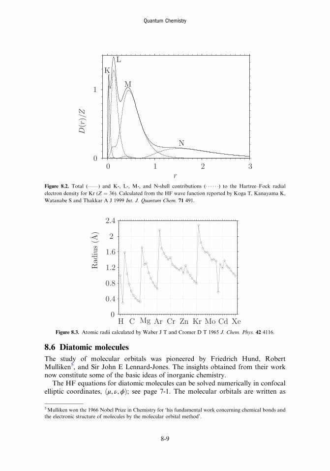
8.6 Diatomic moleculesThe study of molecular orbitals was pioneered by Friedrich Hund, RobertMulliken5, and Sir John E Lennard-Jones. The insights obtained from their worknow constitute some of the basic ideas of inorganic chemistry.

The HF equations for diatomic molecules can be solved numerically in confocalelliptic coordinates, ðμ, ν,ϕÞ; see page 7-1. The molecular orbitals are written as

5Mulliken won the 1966 Nobel Prize in Chemistry for ‘his fundamental work concerning chemical bonds andthe electronic structure of molecules by the molecular orbital method’.

00

1

1

2 3r

D(r

)/Z

KL

M

N

Figure 8.2. Total (——) and K-, L-, M-, and N-shell contributions () ) ) ) ) )) to the Hartree–Fock radialelectron density for Kr (Z ¼ 36). Calculated from the HF wave function reported by Koga T, Kanayama K,Watanabe S and Thakkar A J 1999 Int. J. Quantum Chem. 71 491.

0

0.4

0.8

1.2

1.6

2.4

2

H C Mg Ar Cr Zn Kr Mo Cd Xe

Rad

ius

(A)

Figure 8.3. Atomic radii calculated by Waber J T and Cromer D T 1965 J. Chem. Phys. 42 4116.

Quantum Chemistry

8-9

φðμ, ν,ϕÞ ¼ f ðμ, νÞΦmðϕÞ, where ΦmðϕÞ is a particle-on-a-ring wave function(equation (5.4)) and m ¼ 0, * 1, . . . for σ, π, . . . MOs, respectively. Homonucleardiatomic molecules have D1h symmetry, and their orbitals can be assigned thesymmetry labels 1σg, 1σu, 2σg, 2σu, . . . , just as in Hþ

2 . Figure 8.4 shows the orbitalenergies of the diatomics from B2 to F2. The ordering of the levels is almost the sameas in Hþ

2 (see section 7.6) except that the 3σg and 1πu energies cross twice with 1πubeing lower in B2, C2 and F2, and 3σg being lower in N2 and O2.

The content of figure 8.4 can be summarized by writing down the electronconfigurations. For example, the configuration of C2 is written as1σ2g1σ

2u2σ

2g2σ

2u1π

2ux1π

2uy. It is common to use 1π4u as shorthand for 1π2ux1π

2uy. In

inorganic chemistry textbooks, the numbering is sometimes changed to omit theMOs that contain the core electrons; as a consequence, 1σg in H2, 2σg in Li2, and 3σgin N2 may all be confusingly called 1σg.

The B2 and O2 molecules have two unpaired electrons in their highest occupied πMOs and are therefore paramagnetic. The correct prediction of the paramagnetismof O2 by the MO theory was one of its earliest major successes. A nominal bondorder is given by the number of bonding electron pairs minus the number of

B2 C2 N2 O2 F2

1σg

1σu

2σg

2σu

1πu

3σg

1πg

3σu

Figure 8.4. MO energy level diagram for homonuclear diatomics. The energies are not to scale; the 1σg and 1σuenergies are far lower than the energies of the valence MOs.

Quantum Chemistry

8-10

antibonding electron pairs. Bond orders of 1, 2, and 3 correspond to single, double,and triple bonds, respectively. Figure 8.5 shows that, for the second-period A2

molecules, the greater the bond order, the shorter the bond length and the greater thedissociation energy. Figure 8.4 suggests that Be2 and Ne2 have a bond order of zeroand are not stable molecules. In reality, these molecules are very weakly bound byvan der Waals forces.

8.7 The Kohn–Sham modelThe HF model is useful but also has severe limitations. In section 8.4 we saw thatthere is a residual error of 111 kcal mol#1 in the ionization energy of the heliumatom. Further refinement of the He orbital by using a basis set of three or moreexponential (Slater-type) functions does not help. A 5 × 5 matrix HF calculation ofthis type leads to an energy E ¼ #2:861 68 Eh, which is not much better than theenergy obtained with two functions. Unfortunately, this is the best energy that canbe obtained with a HF wave function. Moreover, the breaking of a bond is verypoorly described by the HF model if both the resulting fragments are open-shellspecies. For example, figure 8.6 shows that the HF potential energy curve for H2

diverges from the exact one as the bond is broken.The HF model wave function is unable to describe the instantaneous, short-range,

dynamical correlation of the motion of the electrons that keeps them apart. It helps tothink of electron correlation as creating a Coulomb hole or bubble around eachelectron in which the probability of finding another electron with opposite spin isgreatly reduced. We now turn to the Kohn–Sham (KS) model because it improvesupon the HF model and creates a Coulomb hole around each electron. The KS modelstems from the 1951 work of John Slater who was trying to simplify the HFmodel. Hereplaced the exchange operator K in the HF equations (8.13) by an effective exchangepotential of the form vxð~rÞ ¼ c ρð~rÞ1=3, where c is a constant. To understand the idea

0

100

100

120

140

160200

B2B2 C2C2 N2N2 O2O2 F2F2

Re

(pm

)

De

(kca

lmol

–1)

Figure 8.5. Bond lengths Re and dissociation energies De. The nominal bond order is 1, 2, 3, 2, and 1 forB2, C2, N2, O2, and F2, respectively.

Quantum Chemistry

8-11

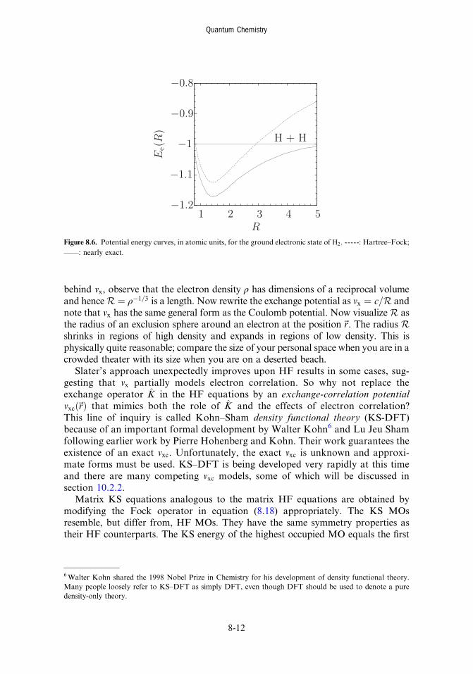
behind vx, observe that the electron density ρ has dimensions of a reciprocal volumeand henceR ¼ ρ#1=3 is a length. Now rewrite the exchange potential as vx ¼ c=R andnote that vx has the same general form as the Coulomb potential. Now visualizeR asthe radius of an exclusion sphere around an electron at the position~r. The radius Rshrinks in regions of high density and expands in regions of low density. This isphysically quite reasonable; compare the size of your personal space when you are in acrowded theater with its size when you are on a deserted beach.

Slater’s approach unexpectedly improves upon HF results in some cases, sug-gesting that vx partially models electron correlation. So why not replace theexchange operator K in the HF equations by an exchange-correlation potentialvxcð~rÞ that mimics both the role of K and the effects of electron correlation?This line of inquiry is called Kohn–Sham density functional theory (KS-DFT)because of an important formal development by Walter Kohn6 and Lu Jeu Shamfollowing earlier work by Pierre Hohenberg and Kohn. Their work guarantees theexistence of an exact vxc. Unfortunately, the exact vxc is unknown and approxi-mate forms must be used. KS–DFT is being developed very rapidly at this timeand there are many competing vxc models, some of which will be discussed insection 10.2.2.

Matrix KS equations analogous to the matrix HF equations are obtained bymodifying the Fock operator in equation (8.18) appropriately. The KS MOsresemble, but differ from, HF MOs. They have the same symmetry properties astheir HF counterparts. The KS energy of the highest occupied MO equals the first

1 2 3 4 5

−1

−0.8

−0

e

.9

−1.1

−1.2

R

E(R

)

H + H

Figure 8.6. Potential energy curves, in atomic units, for the ground electronic state of H2. -----: Hartree–Fock;——: nearly exact.

6Walter Kohn shared the 1998 Nobel Prize in Chemistry for his development of density functional theory.Many people loosely refer to KS–DFT as simply DFT, even though DFT should be used to denote a puredensity-only theory.

Quantum Chemistry

8-12

ionization energy of the molecule. Using KS orbitals in equation (8.12) gives theelectron density. However, the Slater determinant of KS orbitals is not an accuratewave function for the system of interest. Hence, it is not known how to use KS–DFTcorrectly for molecular properties that depend on quantities other than the energyand electron density.

Problems (see appendix B for hints and solutions)8.1 Using atomic units, write down the electronic Hamiltonian for the Liþ cation.Explain the physical meaning of each term.

8.2 Why is it wrong to use ½1sð1Þ1sð2Þ þ 1sð1Þ1sð2Þ'=ffiffiffi2

pas an approximate wave

function for the ground state of the helium atom?

8.3 A Slater determinant satisfies the Pauli principle. So what is wrong with usingj1s1s1sj for the ground state of the Beþ cation?

8.4 Consider an excited (triplet) state of the helium atom which has the configu-ration 1s2s and both electrons have β spin. Set up an orbital-model wave functionthat satisfies the Pauli postulate for this excited state. Write your wave function inthe form of (a) a 2 × 2 determinant, and (b) a spatial function multiplied by a spinfunction.

8.5 In the compact notation of page 8-3, write down a Slater determinant whichcould be used to represent the ground-state wave function of the boron atom in(a) the ROHF method, and (b) the UHF method.

8.6 The energies of the occupied molecular orbitals, 1a1, 2a1, and the triplydegenerate 1t2, of CH4 are #11:20, #0:93 and #0:54 Eh, respectively. Estimate theionization energy of CH4.

8.7 Consider the ground state of a system containing two electrons and a nucleus ofatomic number Z. If we use the Slater determinant of equation (8.9) with thehydrogen-like 1s function of equation (8.3) as the trial wave function in a variationalcalculation, we find E ¼ ζ2 #2Zζ þ 5ζ=8.(a) Find the ζ that should be used without using a specific value for Z. Justify your

answer. For He (Z ¼ 2), your answer should agree with the correspondingresult in section 8.1.

(b) What is the value of the ground-state energy predicted if the above ζ is used?Do not use a specific value for Z at this stage.

(c) Compare the ground-state energy of the H# anion (Z ¼ 1) predicted by thiscalculation with that of the hydrogen atom. What does this lead you to expectabout the stability of H#?

8.8 How many peaks should one see in the photoelectron spectrum of the Ar atom?Explain your answer.

8.9 Use figure 8.4 to write the ground-state electron configurations of O2 and Oþ2 .

Which should have the longer bond length and why?

Quantum Chemistry

8-13

8.10 Write the ground-state electron configuration of Li2. Draw the MO energy-level diagram and sketch the occupied MOs. What is the nominal bond order?Would Liþ2 be more or less strongly bound than Li2?

8.11 Write the ground-state electron configuration of Be2. Draw the MO energy-level diagram and sketch the occupied MOs. What is the nominal bond order? Whatis the lowest unoccupied molecular orbital (LUMO)?

Quantum Chemistry

8-14

IOP Concise Physics

Quantum ChemistryA concise introduction for students of physics, chemistry, biochemistry and materials science

Ajit J Thakkar

Chapter 9

Qualitative MO theory

9.1 The H€uckel modelIn 1930, Erich H€uckel proposed a simple model for the π MOs and energies1 ofplanar conjugated hydrocarbons; the insights his model provides have permeatedorganic chemistry. The H€uckel model remains important although far moresophisticated calculations are possible now.

The H€uckel model is ‘obtained’ from the HF model as follows.1. All σ electrons are neglected except insofar as they affect parameters of the

method. This means that all hydrogen atoms are ignored.2. The basis set for a planar hydrocarbon with N carbon atoms is chosen to be

one 2pπ AO on each carbon atom. If the hydrocarbon is in the xy-plane,these are the 2pz AOs. Thus the kth MO is given by

φk ¼ c1kp1 þ c2kp2 þ # # # þ cNkpN ð9:1Þ

where pi is the AO on carbon i, and the cik are expansion coefficients.3. The elements of the F and S matrices appearing in the matrix HF equations

(8.17) are assigned values instead of being calculated. All overlap is neglectedby setting Sij ¼ 1 when i ¼ j, and Sij ¼ 0 otherwise2. Thus, the H€uckeloverlap matrix is an N ×N identity matrix I; that is S ¼ I. This implies thatthe normalization condition for the H€uckel MO of equation (9.1) is simply

c21k þ c22k þ # # # þ c2Nk ¼ 1: ð9:2Þ

1 The MOs of planar molecules are called σ or π, respectively, depending on whether they remain unchanged orchange sign upon reflection in the molecular plane. Unfortunately, this usage is entrenched in chemistryalthough it is inconsistent with symmetry conventions. Note that degeneracy is not implied by the π label in thiscontext.2 In fact, if the carbon atoms i and j are separated by a typical CC bond distance, then the overlap betweentheir 2pπ orbitals is Sij & 0:25. However, inclusion of overlap does not change the results by huge amounts.

doi:10.1088/978-1-627-05416-4ch9 9-1 ª Morgan & Claypool Publishers 2014

4. A diagonal Fock matrix element Fii is roughly the energy of an electron inthe 2pπ AO of carbon i. They are all made equal because the carbon atoms inconjugated hydrocarbons are nearly equivalent: Fii & α. Thus, the diagonalpart of the H€uckel F is simply α I.

5. If carbon atoms i and j are not bonded to each other, their interaction issmall, and the matrix elements Fij ¼ Fji & 0. If the carbon atoms i and j arebonded to each other, then H€uckel sets the matrix elements Fij ¼ Fji to aninteraction energy, β. Moreover, this negative value β is used for all bondedpairs because all carbon atoms in conjugated hydrocarbons are nearlyequivalent and all CC bond lengths are nearly equal. Thus, the off-diagonalpart of the H€uckel F matrix is βA in which the elements of A are given byAij ¼ 1 if atoms i and j are bonded and by Aij ¼ 0 otherwise. A is called theadjacency matrix because the only information it contains is the connectivityof the molecule—which carbons are bonded to which other carbons. Puttingthe diagonal and off-diagonal parts together, the Fock matrix becomesF ¼ α Iþ βA. The H€uckel F reflects the permutational symmetry of A butdoes not contain any geometrical information. For example, in cyclobuta-diene with atoms numbered sequentially,

F ¼

α β 0 β

β α β 0

0 β α β

β 0 β α

2

6664

3

7775 ¼ α

1 0 0 0

0 1 0 0

0 0 1 0

0 0 0 1

2

6664

3

7775þ β

0 1 0 1

1 0 1 0

0 1 0 1

1 0 1 0

2

6664

3

7775:

6. The π-electron energy Eπ is taken as the sum of the orbital energies.

Inserting the H€uckel S and F into the matrix equations (8.17) leads to

ðα Iþ βAÞCk ¼ EkICk for k ¼ 1, . . . ,N: ð9:3Þ

Subtracting α ICk from both sides of equation (9.3), using ICk ¼ Ck, collectingterms, and dividing both sides by β, we find

ACk ¼ xkCk for k ¼ 1, . . . ,N ð9:4Þ

in which xk ¼ ðEk ' αÞ=β. F and A have the same eigenvectors and the H€uckelorbital energies are obtained from the eigenvalues of A using

Ek ¼ αþ xkβ for k ¼ 1, . . . ,N: ð9:5Þ

Equation (9.4) provides a route to the H€uckel orbital energies and MOs without theneed to assign numerical values to α and β.

Quantum Chemistry

9-2

9.2 CumulenesA cumulene is a conjugated non-branched chain of N carbons, HðCHÞNH.

1

2

N3

N-1

Ethene, the allyl radical, and 1,3-butadiene are cumulenes with N ¼ 2, 3, and 4,respectively. The H€uckel energies and MOs are shown in figure 9.1 for ethene. As inchapter 7, the positive lobes of the MOs are shaded. φ1 is a bonding MO because itleads to a build-up of charge between the nuclei, whereas φ2 has a nodal plane per-pendicular to the C¼C bond and is antibonding. Hence, the orbital energy αþ β is thelower one confirming that β< 0. The total π-electron energy is Eπ ¼ 2E1 ¼ 2ðαþ βÞ.

Next consider the orbital energies shown in figure 9.2 for butadiene. The fourπ-electrons occupy the two lowest energy levels. Thus, Eπ ¼ 2E1 þ 2E2 ¼ 4αþ 4:48β.If the two π-bonds were non-interacting, then we would expect a π-electron energytwice that of ethene—that is, 4ðαþ βÞ. The difference between the H€uckel Eπ andits hypothetical non-interacting counterpart is called the delocalization energy, ΔEdl.For butadiene, ΔEdl ¼ Eπ ' 4ðαþ βÞ ¼ 0:48β. The delocalization energy is due toconjugation.

The sketches of the MOs in figure 9.2 follow from the MO coefficients noting thatthe carbon atoms are numbered from left to right. The shaded lobes of the atomicp orbitals are positive and the unshaded ones are negative. The size of each atomicorbital is proportional to its coefficient in that MO. The lowest-energy MO (φ1) isbonding between each pair of adjacent carbons. The next MO, φ2, has two bondinginteractions (between carbons 1–2 and 3–4) and one antibonding interaction

2 = α − β

1 = α + β

ϕ2 = 0.71 (p1 − p2)

ϕ1 = 0.71 (p1 + p2)

Figure 9.1. H€uckel energy levels and MOs for ethene.

4 = α − 1.62β

1 = α + 1.62β

3 = α − 0.62β

2 = α + 0.62β

ϕ4 = 0.37p1 − 0.60p2 + 0.60p3 − 0.37p4

ϕ1 = 0.37p1 + 0.60p2 + 0.60p3 + 0.37p4

ϕ2 = 0.60p1 + 0.37p2 − 0.37p3 − 0.60p4

ϕ3 = 0.60p1 − 0.37p2 − 0.37p3 + 0.60p4

Figure 9.2. H€uckel energies and MOs for 1,3-butadiene.

Quantum Chemistry

9-3

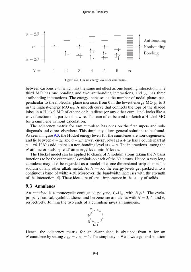
between carbons 2–3, which has the same net effect as one bonding interaction. Thethird MO has one bonding and two antibonding interactions, and φ4 has threeantibonding interactions. The energy increases as the number of nodal planes per-pendicular to the molecular plane increases from 0 in the lowest energy MO φ1 to 3in the highest-energy MO φ4. A smooth curve that connects the tops of the shadedlobes in a H€uckel MO of ethene or butadiene (or any other cumulene) looks like awave function of a particle in a wire. This can often be used to sketch a H€uckel MOfor a cumulene without calculation.

The adjacency matrix for any cumulene has ones on the first super- and sub-diagonals and zeroes elsewhere. This simplicity allows general solutions to be found.As seen in figure 9.3, the H€uckel energy levels for the cumulenes are non-degenerate,and lie between αþ 2β and α' 2β. Every energy level at αþ xβ has a counterpart atα' xβ. IfN is odd, there is a non-bonding level at E ¼ α. The interactions among theN atomic orbitals ‘spread’ an energy level into N levels.

The H€uckel model can be applied to chains of N sodium atoms taking the N basisfunctions to be the outermost 3s orbitals on each of the Na atoms. Hence, a very longcumulene may also be regarded as a model of a one-dimensional strip of metallicsodium or any other alkali metal. As N ! 1, the energy levels get packed into acontinuous band of width 4jβj. Moreover, the bandwidth increases with the strengthof the interaction jβj. These ideas are of great importance in the study of solids.

9.3 AnnulenesAn annulene is a monocyclic conjugated polyene, CNHN , with N ⩾ 3. The cyclo-propenyl radical, cyclobutadiene, and benzene are annulenes with N ¼ 3, 4, and 6,respectively. Joining the two ends of a cumulene gives an annulene.

1

2

N-1N

Hence, the adjacency matrix for an N-annulene is obtained from A for anN-cumulene by setting A1N ¼ AN1 ¼ 1. The simplicity of A allows a general solution

N = 1 2 3 4 5 6 ∞

α + 2β

α − 2β

α

Bonding

AntibondingNonbonding

Figure 9.3. H€uckel energy levels for cumulenes.

Quantum Chemistry

9-4

to be found. Note from figure 9.4 that all the annulenes have a non-degenerate levelat αþ 2β followed by doubly degenerate levels; when N is even, there is also a non-degenerate level at α' 2β. When N is even, every energy level at αþ xβ has acounterpart at α' xβ. This pairing of energy levels does not occur in annulenes withodd N. Observe that as N ! 1, the doubly degenerate energy levels get packed intoa continuous band of width 47β7.

There is a striking similarity between the H€uckel orbital energies for annulenesand the energy levels of a particle on a ring (see figure 5.2 on page 5-3). To have astable filled-subshell π-electron configuration, the number of π electrons must beNπ ¼ 2þ 4m for m ¼ 0, 1, . . .. This gives H€uckel’s 4mþ 2 rule: monocyclic conju-gated systems are most stable if they contain 4mþ 2 π electrons. Benzene and thecyclopentadienyl anion satisfy the 4mþ 2 rule with m ¼ 1 because they have sixπ electrons. Such molecules are called aromatic. The H€uckel model predicts thatannulenes with 4m π electrons are highly unstable diradicals. Monocyclic conjugatedhydrocarbons with 4m π electrons are called anti-aromatic.

The H€uckel orbital energies and MOs of benzene are shown in figure 9.5where the carbons are numbered sequentially around the ring. The lowest energyMO φ1 is bonding between each pair of adjacent carbons. The φ2 MO has fourbonding interactions (between carbons 1–2, 1–6, 3–4, and 4–5) and two anti-bonding interactions (between carbons 2–3 and 5–6) which has the same neteffect as two bonding interactions. Its degenerate partner φ3 has two bondinginteractions (between carbons 2–3 and 5–6) and no antibonding interactions. Thedegenerate MOs, φ4 and φ5, have one nodal plane perpendicular to the molecularplane. The MO energy increases with increasing number of nodal planes per-pendicular to the molecular plane; there are 0 nodal planes of this type in φ1 and3 in the k ¼ 6 MO.

The H€uckel π-electron energy for benzene is Eπ ¼ 2ðαþ 2βÞ þ 4ðαþ βÞ ¼6αþ 8β. If the three π bonds were non-interacting, then we would expect aπ-electron energy three times that of ethene—that is, 6ðαþ βÞ. The delocalizationenergy is then ΔEdl ¼ 6αþ 8β ' 6ðαþ βÞ ¼ 2β. This large delocalization energygives benzene an extra stability. It is precisely this stability that is predicted byH€uckel’s 4mþ 2 rule.

N = 3 4 5 6 ∞

α + 2β

α − 2β

α

Bonding

Nonbonding

Antibonding

Figure 9.4. H€uckel energy levels for annulenes.

Quantum Chemistry

9-5

9.4 Other planar conjugated hydrocarbonsWe now turn to other hydrocarbons. The H€uckel energy levels for planar conjugatedhydrocarbons with one or more tertiary carbon atoms bonded to three other carbonsdo not all lie between αþ 2β and α' 2β; for example, the lowest orbital energy forstyrene (phenylethene) is at αþ 2:14β. However, it is true that the H€uckel energylevels for any planar conjugated hydrocarbon always lie between αþ 3β and α' 3β.

Conjugated hydrocarbons which contain a ring with an odd number of atoms aresaid to be non-alternant. All other conjugated hydrocarbons are called alternanthydrocarbons. For any alternant hydrocarbon, it is always possible to place labels onsome of the carbons in such a manner that no two neighbors are both labeled or bothunlabeled. Such a labeling is impossible for a non-alternant hydrocarbon.

The pairing theorem states that for each H€uckel energy level at αþ xβ, analternant hydrocarbon has another one at α' xβ. We have seen this for thecumulenes in section 9.2 and for the alternant annulenes (those with an even numberN of carbon atoms) in section 9.3. A simple consequence of the pairing theorem is

ϕ1

ϕ2

ϕ4

ϕ6

α + 2β

α − 2β

α + β

α − β

ϕ3

ϕ5

ϕ6 = (p1 − p2 + p3 − p4 + p5 − p6) /√

6ϕ5 = (p2 − p3 + p5 − p6) /2

ϕ4 = (2p1 − p2 − p3 + 2p4 − p5 − p6) /√

12ϕ3 = (p2 + p3 − p5 − p6) /2

ϕ2 = (2p1 + p2 − p3 − 2p4 − p5 + p6) /√

12

ϕ1 = (p1 + p2 + p3 + p4 + p5 + p6) /√

6Figure 9.5. H€uckel energy levels and MOs for benzene.

Quantum Chemistry

9-6

that the sum of all the H€uckel energies, occupied and unoccupied, isNα for alternanthydrocarbons with N carbon atoms. This result is also true for non-alternanthydrocarbons even though the pairing theorem is inapplicable; see problem 9.10.

Several computer programs are freely available for performing numerical cal-culations to obtain detailed solutions of the H€uckel model for conjugated hydro-carbons other than cumulenes and annulenes. As an example, figure 9.6 shows theresults of a computer calculation on methylenecyclopropene. The pairing theoremdoes not apply to this molecule because it is a non-alternant hydrocarbon. Hence theenergy levels are not placed symmetrically with respect to α. Nevertheless, the sumof all four orbital energies is precisely 4α. Carbon atom 3 is bonded to three othercarbons and hence the lowest energy level is lower than αþ 2β, unlike in anycumulene or annulene. The two lowest energy levels are doubly occupied and thetotal π energy is Eπ ¼ 4αþ 4:96β corresponding to a delocalization energy ofΔEdl ¼ Eπ 'Nπðαþ βÞ ¼ 0:96β. The delocalization energy is due to conjugation.φ1 is bonding over the entire molecule. φ2 has bonding character between carbons1–2 and 3–4 but is antibonding between carbons 1–3 and 2–3, making it almostnon-bonding overall as reflected by the closeness of its energy to α.

9.5 Charges, bond orders, and reactivityEach term on the left-hand side of the normalization condition, equation (9.2), forH€uckel MO φk pertains to a different carbon atom; one may interpret jcjk j2 as thefraction of an electron in φk that resides on atom j. Adding up a contribution fromeach MO, weighted by the number of electrons in it, gives the π-electron population(or π charge) qj of atom j. Thus, we write

qj ¼ m1jcj1j2 þm2jcj2j2 þ # # # þmN jcjN j2 ð9:6Þ

in whichmk is the number of electrons in the kth MO and cjk is the coefficient of pj inthe kth MO. For example, the population on atom 4 in methylenecyclopropene,figure 9.6, is q4 ¼ 2× 0:282 þ 2× ð'0:82Þ2 ¼ 1:49 electrons. Similarly, we find thatq1 ¼ q2 ¼ 0:82 and q3 ¼ 0:88 electrons. Obviously, unoccupied MOs do not con-tribute to qj because they have mk ¼ 0. The sum of the populations on all the atomsequals the total number of π electrons in the molecule (four in this case).

1 2

3

4

α − 1.48βα − 1.00β

α + 2.17β

α + 0.31β

ϕ4 = 0.30p1 + 0.30p2 − 0.75p3 + 0.51p4

ϕ3 = 0.71p1 − 0.71p2

ϕ1 = 0.52p1 + 0.52p2 + 0.61p3 + 0.28p4

ϕ2 = 0.37p1 + 0.37p2 − 0.25p3 − 0.82p4

Figure 9.6. H€uckel energies and MOs for methylenecyclopropene.

Quantum Chemistry

9-7

The π-electron populations are indicators of reactivity. An electrophile is mostlikely to attack the carbon with the largest π charge whereas a nucleophile is mostlikely to attack the carbon with the smallest π charge. The π-electron populationscalculated above for methylenecyclopropene show a build-up of electron density atthe methylene carbon, making it a prime target for electrophilic attack.

Unfortunately, π charges are useless as reactivity indices for alternant hydro-carbons because all the carbons have the same π population. An electrophile is mostlikely to seek electrons from the highest occupied MO (HOMO), and hence therelevant measure of reactivity is the π charge in the HOMO given by c2j,HOMO.Similarly, a nucleophile is most likely to donate electrons to the lowest unoccupiedMO (LUMO) and the reactivity of carbon j to nucleophilic attack can be measuredby c2j,LUMO. These reactivity indices based on the frontier orbitals, the HOMO andLUMO, are also used as additional reactivity indices for non-alternant hydrocarbons.

Charles Coulson generalized equation (9.6) by defining the π-bond order of thebond between a pair of bonded carbon atoms i and j as follows:

Pij ¼ m1ci1cj1 þm2ci2cj2 þ # # # þmNciNcjN : ð9:7Þ

This definition leads to a π-bond order of 1 in ethene as expected. The Lewis structurefor butadiene has perfectly localized, alternating double and single bonds; in otherwords, it shows π-bond orders of P12 ¼ 1, P23 ¼ 0 and P34 ¼ 1. By contrast, substi-tuting MO coefficients from figure 9.2 into equation (9.7), the H€uckel π-bond ordersare found to be P12 ¼ 2× 0:37× 0:60þ 2× 0:60× 0:37 ¼ 0:89, P23 ¼ 2× 0:60×0:60þ 2× 0:37× ð'0:37Þ ¼ 0:45, and P34 ¼ 0:89. Comparison with the Lewis bondorders shows that the bond between the central carbons has acquired some πcharacter at the expense of the terminal bonds; in other words, the π electronsare delocalized due to conjugation. General chemistry textbook descriptions of the‘resonance’ between two equivalent Kekulé structures suggest that the CC π-bondorders in benzene should be close to 1=2. The H€uckel model predicts the CC π-bondorders in benzene to be 2=3 indicating that π-electron delocalization strengthens all theCC bonds. The π-bond order between carbon atoms 1 and 3 in methylenecyclo-propene is P13 ¼ 0:45 showing π-electron delocalization in the three-membered ring.The total bond order is 1þ Pij since there is also a σ bond between every pair ofbonded carbons.

Molecular geometry plays no role in the H€uckel model because it uses onlyconnectivity information. For example, there is no difference between cis- and trans-butadiene in the H€uckel model because both isomers have the same connectivity.However, Coulson found a relationship between H€uckel model π-bond orders Pjk

and experimental bond lengths Rjk :

Rjk & Rs 'PjkðRs ' RdÞ

Pjk þ 0:765ð1' PjkÞð9:8Þ

in which Rs ¼ 154 pm and Rd ¼ 134 pm are typical CC single and double bondlengths, respectively. Equation (9.8) is set up to predict correctly that Rjk ¼ Rs whenPjk ¼ 0 and Rjk ¼ Rd when Pjk ¼ 1. This simple empirical formula gives useful

Quantum Chemistry

9-8

predictions of CC bond lengths in conjugated hydrocarbons. For example, itcorrectly predicts CC bond lengths of 140 pm in benzene. Formula (9.8) gives aC2–C3 bond length of 144 pm in butadiene to be compared with the experimentalvalue of 146 pm.

Reaction with a free radical should proceed with the radical forming a bond to acarbon. This will be easiest with carbons which have the greatest bonding capacityleft over after accounting for the bonds that are initially present in the molecule.Thus, the free valence is the difference between the maximum π bonding a carbonatom can have and the amount of π bonding it actually has in the molecule prior toreaction. The amount of π bonding (Bk) at atom k is measured by the sum of theorders of all the π bonds involving the atom. Coulson defined the free valence indexof carbon k as

fk ¼ffiffiffi3

p' Bk ð9:9Þ

in whichffiffiffi3

pis the largest possible H€uckel value3 of Bk for any trigonally bonded

carbon. For example, using the π-bond orders calculated on page 9-8, the freevalence of carbon atom 1 in butadiene is f1 ¼

ffiffiffi3

p' P12 ¼ 1:73' 0:89 ¼ 0:84

whereas the carbon atom 2 has f2 ¼ffiffiffi3

p' P12 ' P23 ¼ 1:73' 0:89' 0:45 ¼ 0:39.

Check that f3 ¼ f2 and f4 ¼ f1. The free valence values correctly predict that theprimary carbons are more vulnerable to free radical attack than the secondarycarbons.

By and large, the various reactivity indices provide very simple and usefulmeasures of reactivity. However, none of these reactivity indices is perfect. Some-times the different indices predict different things. One must expect a model assimple as the H€uckel model to have shortcomings.

9.6 The H€uckel model is not quantitativeThe H€uckel method provides very useful qualitative results for conjugated hydro-carbons. The 4mþ 2 rule is an outstanding example of its success. Unfortunately,attempts to use the H€uckel model quantitatively by assigning numerical values to αand β revealed that different values are required for different properties to agree withexperiment. Hence, quantitative use of the H€uckel model has been abandoned.

An extended H€uckel method that includes all valence electrons plays an analo-gous role for molecules of all types, organic and inorganic. The method providesqualitative results such as the nodal structure and symmetries of molecular orbitals.The Woodward–Hoffmann4 rules used in organic chemistry were based on suchcalculations. It is not, however, a quantitative method like those discussed inchapter 10.

3 The maximal value of Bk ¼ffiffiffi3

p, and hence fk ¼ 0, is found for the central carbon atom in the diradical

CðCH2Þ3.4 Robert Woodward won the 1965 Nobel Prize in Chemistry for his work on organic synthesis, and KenichiFukui and Roald Hoffmann shared the 1981 Nobel Prize in Chemistry for their work on quantum theories ofchemical reactions.

Quantum Chemistry

9-9

Problems (see appendix B for hints and solutions)9.1 Write down the adjacency matrix for (a) butadiene (C4H6) with the atomsnumbered sequentially from left to right, and (b) benzene (C6H6) with the atomsnumbered sequentially around the ring.

9.2 Prove that the orthogonality conditionRφiφj dτ ¼ 0 for i 6¼ j can be expressed

in terms of the H€uckel MO coefficients as

c1ic1j þ c2ic2j þ # # # þ cNicNj ¼ 0 for i 6¼ j:

9.3 Show that the HOMO and LUMO in figure 9.2 are orthonormal.

9.4 Use results from section 9.2 and section 9.3 to draw a π-orbital energy leveldiagram for (a) cyclo-octatetraene and (b) octatetraene.

Which of these molecules would you expect to be more stable? Why?

9.5 Which of C5Hþ5 , C5H5 and C5H

'5 is expected to be the most stable? How does

this help to understand the structure of ferrocene, FeðC5H5Þ2?

9.6 Given α ¼ '6:15 eV and β ¼ '3:32 eV, predict the ionization energy forbenzene and compare it with the experimental value of 9.4 eV.

9.7 A student performed a H€uckel calculation on fulvene.(a) She found that C3, C4, and C5 had π-electron populations of 1.073, 1.092,

and 1.047, respectively. What were the π-electron populations on C1, C2,and C6?

1

2 3

456

(b) Use these π-electron populations to predict which carbon atom a nucleophile ismost likely to attack. Explain your choice.

(c) The student found π-bond orders of 0.76, 0.45, 0.78, and 0.52 for the C6–C5,C5–C4, C4–C3, and C3–C2 bonds, respectively. Calculate the free valence indexfor C2.

(d) Use π-bond orders and free valence indexes to predict which carbon atom a freeradical would be most likely to attack. Explain your choice.

Quantum Chemistry

9-10

9.8 A lone-pair electron on theO atom inH2C¼CH–CH¼O is promoted to the lowestunoccupied molecular orbital (LUMO). Assuming that the π-MOs of prop-2-enoneare the same as in butadiene, explainwithMOdiagrams butwithout calculationswhichCC bond you would expect to become longer and which shorter as a result of thistransition, and why.

9.9 Calculate the π-bond orders of the C1–C2 and C2–C3 bonds for butadiene usingequation (9.7) and the H€uckel MOs given in figure 9.2. Check against section 9.5.Suppose an electron moves from the π HOMO to the π LUMO in butadiene. Findthe π-bond orders for this excited state.

9.10 Calculate the trace (sum of diagonal elements) of the H€uckel F matrix. Whatdoes this tell us about the energy levels?

9.11 Alice found a pair of degenerate H€uckel MOs for cyclobutadiene:

φa ¼ ðp1 ' p3Þ=ffiffiffi2

pand φb ¼ ðp2 ' p4Þ=

ffiffiffi2

p:

However, Jim thought that the same pair of degenerate MOs were given by:

φc ¼ ðp1 ' p2 ' p3 þ p4Þ=2 and φd ¼ ðp1 þ p2 ' p3 ' p4Þ=2:

They were both right. Explain how that can be true.

Quantum Chemistry

9-11

IOP Concise Physics

Quantum ChemistryA concise introduction for students of physics, chemistry, biochemistry and materials science

Ajit J Thakkar

Chapter 10

Computational chemistry

10.1 Computations are now routineComputations complement experimental work. They are used to predict quantitiesthat are too hard, expensive, time-consuming, or hazardous to measure. For example,the structure of a transition state is easier to calculate than measure. Calculations canguide the design of experimental work. For example, pharmaceutical companiesdeveloping new drugs routinely use computational methods to screen compounds forlikely activity before synthesizing them. Computational methods can predict equi-librium geometries, transition-state structures, dipole moments, barriers to internalrotation, relative energies of isomers, enthalpies of reaction and formation, and manyother properties. It is a rare chemical problem where computational chemistry is of nohelp at all.

The HF and KS methods described in chapter 8 have been implemented in manycomputer programs, such as GAMESS, ORCA and GAUSSIAN. The programs can be runon cheap commodity computers. Virtually anyone can easily learn how to performquantum chemical calculations with them. However, it is harder to learn to recog-nize problems that are amenable to computation, choose methods appropriate to theproblem, and assess the results. The latter tasks are difficult because many choiceshave to be made. Several books have been written on the subject.

This chapter summarizes a minimal amount of essential material about quantumchemical methods to help you understand papers that use such methods. Anintroduction to basis set selection is given in section 10.2. The choice of functional ina KS-DFT calculation, the handling of heavy atoms, and methods to account forsolvent effects are discussed very briefly in section 10.2. An outline of practicalcomputational strategies and a map of the main methods of current computationalchemistry are given in section 10.3.

doi:10.1088/978-1-627-05416-4ch10 10-1 ª Morgan & Claypool Publishers 2014

10.2 So many choices to be made10.2.1 Selection of a basis set

In the Hþ2 calculations of section 7.1 and section 7.4, the MOs were represented by

linear combinations of atom-centered 1s-type functions ðe#ζrÞ and 2pz-like polar-ization functions ðze#ζrÞ. These functions are special cases of Slater-type functionsdefined by N e#ζrr‘Y‘,m where Y‘,m is a spherical harmonic (section 5.2) and N is anormalization constant; see table 10.1.

Unfortunately, the computation of the required integrals is rather time-consumingfor Slater-type functions. The integrals are greatly simplified if one uses Gaussianfunctions defined byN e#ζr2r‘Y‘,m and listed in table 10.1. However, this leads to a lossof accuracy. A solution that combines computational efficiency and accuracy is to usefixed linear combinations of Gaussians, called contracted Gaussian functions (CGF),with parameters predetermined by atomic calculations or some other prescription.For example, s1 ¼ 0:317 e#0:110 r2 þ 0:381 e#0:406 r2 þ 0:109 e#2:228 r2 is an s-typeCGF.Almost all contemporary calculations use a basis set of CGFs.

A minimal basis set contains one basis function for each type of AO that isoccupied in the ground state of each atom in the molecule. For example, a minimalbasis set contains one s-type basis function for each hydrogen atom in a moleculesince H has one occupied AO (1s). Similarly, a minimal basis set has two s-type andone set of three p-type basis functions for each second-period atom since these atomshave an occupied 1s AO in the core, and occupied 2s and 2p valence AOs1. Thus, aminimal basis set for benzene (C6H6) contains N ¼ 6× 5þ 6× 1 ¼ 36 basis func-tions. A well-known minimal CGF basis set is STO-3G in which the name denotesthat CGF consisting of three Gaussians are used for each AO.

Minimal basis sets are not accurate enough for most purposes and are not usedexcept for very large systems. Instead, minimal basis sets are conceptual buildingblocks for double-zeta (DZ) and split-valence (SV) basis sets. A double-zeta basiscontains twice as many functions as a minimal basis; each function in the minimalbasis set is replaced by two of the same type. We have already seen a double-zetabasis set for He on page 8-7. The description of an atom in a molecule may require

Table 10.1. Slater- and Gaussian-type functions in unnormalized form.

Type Slater Gaussian Type Slater Gaussian

s e#ζr e#ζr2 dxy xy e#ζr xy e#ζr2

px x e#ζr x e#ζr2 dyz yz e#ζr yz e#ζr2

py y e#ζr y e#ζr2 dxz xz e#ζr xz e#ζr2

pz z e#ζr z e#ζr2 dx2#y2 ðx2 # y2Þ e#ζr ðx2 # y2Þ e#ζr2

dz2 ð3z2 # r2Þ e#ζr ð3z2 # r2Þ e#ζr2

1 It is necessary to add p-type basis functions in Li and Be because they have unoccupied 2p-type AOs that arequite close in energy to the occupied 2s AO.

Quantum Chemistry

10-2

p functions of different sizes in different directions because the chemical environ-ment of the atom may be different in different directions.

This cannot be achieved with a minimal basis set but is clearly possible with a DZbasis set. A split-valence basis set is a minimal basis set for the core and a DZ set forthe valence region. A SV set is almost as accurate as a DZ set for many chemicalproperties because they are not affected much by the core electrons. For example, aSV basis set for a second-period atom such as C contains nine CGF: three of s typeand six of p type. Common SV basis sets include the 3-21G, 4-31G, and 6-31G basissets2. The notation 3-21G tells us that each core CGF contains three Gaussians andthere are two valence CGF—one containing two Gaussians and the other containingonly one Gaussian.

The smallest basis sets that offer a good compromise between accuracy andcomputational effort are obtained by adding polarization functions of higher angularmomentum to a DZ or SV basis set. The polarization functions help to describe howthe electron cloud of an atom polarizes (distorts) under the influence of the otheratoms in the molecule. The polarization of an s function by a pz function wasillustrated on page 7-7. The polarization of p-type functions is achieved with d-typefunctions, as shown below.

+

An SV plus polarization (SVP) basis set is an SV basis plus a set of three p-typefunctions on each hydrogen atom, a set of five d-type functions on each B, C, N, O,and F atom, and so on. A popular SVP basis set is the 6-31G** or 6-31G(d,p) set,which consists of a 6-31G set plus polarization functions. Another common SVPbasis set is cc-pVDZ. Sometimes polarization functions are included only on thenon-hydrogen atoms, as in the 6-31G* or 6-31G(d) basis set, to reduce computation.

Calculations on anions and weakly bonded systems require diffuse functions—Gaussians with relatively small exponents. The addition of diffuse functions to a basisset is often denoted by ++ or the ‘aug-’ prefix. For example, the 6-31++G(d,p) basis setconsists of the 6-31G(d,p) basis plus an s-type diffuse function on each H atom, an

2These basis sets and others named in this fashion were developed in the laboratory of John Pople who sharedthe 1998 Nobel Prize in Chemistry ‘for his development of computational methods in quantum chemistry’. Thewidely used GAUSSIAN computer program was developed by his research group.

Quantum Chemistry

10-3

s-type and a set of p-type diffuse Gaussians on each B, C, N, O, and F atom, and so on.The cc-pVDZ set with added diffuse functions is called aug-cc-pVDZ.

Larger basis sets are constructed in a similar manner. For example, one can havevalence triple-zeta basis sets with two sets of polarization functions, as in the 6-311G(2d,2p) basis set. A systematic sequence of basis sets of increasing quality is formedby the cc-pVDZ, cc-pVTZ, cc-pVQZ, cc-pV5Z, and cc-pV6Z sets, and anothersequence is formed by their aug- counterparts. The computer time required to domatrix HF or KS calculations increases with the number of basis functions N as N4.For large molecules, the computational cost increases less rapidly, roughly as N2:7

for HF and KS-DFT, because of the weak coupling between basis functions that arelocated on well-separated atoms.

10.2.2 Selecting a functional

An exchange-correlation potential vxc, or an exchange-correlation energy func-tional3 Exc, has to be specified if KS-DFT calculations are desired. Many functionalsare available but it is probably best to stick to the most heavily used and well-testedones. Functionals of the generalized gradient approximation (GGA) type dependupon both the electron density and its gradient. Popular GGA functionals includethe empirical BLYP and SOGGA functionals and the theoretically better justifiedPW91 and PBE (sometimes called PBEPBE) functionals. Computationally moreexpensive hybrid methods use a mixture of the HF exchange operator K and anapproximate vxc. B3LYP is by far the most widely used hybrid functional althoughPBE0 (sometimes called PBE1PBE) is better justified theoretically. Corrections forvan der Waals (dispersion) forces are now common as in the B3LYP-D3 scheme.Finding better functionals is a high priority in current research; new functionals areproposed almost every month.

10.2.3 Heavy atoms and relativistic effects

The observation that many chemical properties of atoms and molecules are deter-mined primarily by the valence electrons was exploited in the construction ofsmaller, but equally accurate, basis sets on page 10-2. For molecules containingatoms from the fifth period and beyond, that is Rb and heavier atoms, a muchgreater computational saving can be obtained if all terms describing the interactionof the electrons in the core orbitals with each other, with the valence electrons, andwith the nuclei, are simply replaced by an ‘effective core potential’ (ECP), and thenuclear charges Z appearing in the interaction potential between the valence elec-trons and the nuclei are replaced by effective nuclear charges Zeff ¼ Z #Nc, whereNc is the number of core electrons. In addition to the computational savings, ECPscan be made to approximate relativistic effects as well; the latter are important inatoms with a large nuclear charge because the innermost electrons move with aspeed approaching that of light. All this has to be done in a manner that does not

3The two are related by vxcð~rÞ ¼ δExc=δρð~rÞ.

Quantum Chemistry

10-4

violate the Pauli principle. The process of constructing an ECP is complex and wellbeyond the scope of this book.

The choice of Nc is important but not always intuitive. For example, to obtaingood results, it suffices to treat Si ([Ne] 3s23p2) as a 4 valence-electron system but it isnecessary to treat Ti as a 12 valence-electron system ([Ne] 3s23p63d24s2) and not as a4 valence-electron system ([Ar] 3d24s2). ECPs are often available for varying coresizes. It is usually safe to use small-core or medium-core ECPs but large-core ECPsshould be used only with caution. The most commonly used effective core potentialsinclude those from the Los Alamos National Laboratory and the Stuttgart–Dresdencollections.

10.2.4 Accounting for a solvent

All the methods discussed so far relate to molecules in the gas phase but the propertiesof a molecule in solution can be quite different from its gas-phase properties.Reaction-field methods are currently used to include solvent effects. The solvent ismodeled as a continuum of uniform dielectric constant ɛ, and the solute moleculeis placed in a cavity within the solvent field. The simple Onsager model, in which aspherical cavity is used, predicts a non-zero solvent effect only for molecules witha non-zero dipole moment. The polarizable continuummodel is a more sophisticatedmodel in which the cavity is described by a set of interlocking atomic spheres.Reaction-field calculations are routine; the only additional actions required from theuser are to specify the solvent, choose the reaction-field model, and run a calculationto estimate the cavity radius if the Onsager model is to be used.

10.3 Practical calculationsQuantum chemical calculations almost never lead to exact results; we just findinexact solutions to approximate equations. Hence, it rarely makes sense to do just asingle calculation. Instead, a series of calculations must be done to assess thereliability of the results. The size of the molecules and degree of difficulty incomputing the property of interest will determine tactical details, such as the choiceof basis sets and methods. Often, the limitations of the available computer hardwareforce one to settle for a lower level of calculation than one knows, or finds, isrequired to obtain the desired reliability.

The goal of the calculations should determine the computational strategy. If theobject is to understand or predict trends in the variation of a property across a setof molecules, then one should calculate the property using an inexpensive KS-DFTmethod which lies in the middle third of the simplified map of quantum chemicalmethods shown in figure 10.1. It is advisable to calibrate the results by performingor looking up parallel calculations on an additional set of similar molecules forwhich the trend is already known. A KS-DFT computation requires a choice ofboth basis set and functional. The usual notation for a KS-DFT calculation isthe name of the functional followed by a slash followed by the basis set name.For example, one can talk about a B3LYP/6-31G(d) or PBE/cc-pVTZ calculation.Hybrid functionals are often more accurate than GGA varieties, especially for

Quantum Chemistry

10-5

organic molecules. The most commonly reported calculations are of the B3LYP/6-31G(d,p) and B3LYP/6-31+G(d,p) varieties. However, it is more prudent to usePBE or PBE0 for molecules containing several transition metal atoms. A correctionfor dispersion (van der Waals) interactions is often applied to KS-DFT calculations.It is not uncommon to see KS-DFT calculations in a systematically improvingsequence of basis sets.

There are many other ab initio4 methods for finding wave functions better thanthe HF model but they are beyond the scope of this book. The simplest such method,called second-order Møller–Plesset (MP2) perturbation theory, is widely used tocalculate a correction to the HF energy in terms of integrals that involve all theoccupied and virtual HF orbitals. In situations where KS-DFT is known to produceresults of uneven quality, it is recommended to do MP2 calculations for calibration.A similar notation is used for MP2 computations—for example, one writes MP2/cc-pVTZ or MP2/6-311G(2d,2p). MP2 calculations typically take only twice as long asKS-DFT calculations. If both KS-DFT and MP2 results turn out to be not accurateenough for one’s purposes, then one must do systematic ab initio calculations asdescribed in the next paragraph.

If the object is to calculate as accurate a value as possible for some property of asmall molecule, then it is appropriate to perform a sequence of computations inwhich the level of both the method and the basis set are systematically increased

Hartree–Fock

Parameterize

THE,lekcuH:evitatilauQ

Older: AM1, PM3

Newer: RM1, PM6, PM7

Modify F (KS-DFT)

LDA

GGA: PBE, BLYP, SOGGA, . . .

Hybrid: PBE0, B3LYP, MPW3LYP, M06, . . .

Build upon

Perturbative: MP2, MP3, . . .

Non-linear: CCSD, CCSD(T), . . .

Variational: MCSCF, CI, MRCI, . . .

Figure 10.1. A schematic map of the quantum chemical forest.

4Ab initio derives from Latin and means ‘from first principles’.

Quantum Chemistry

10-6

until the results stabilize. KS-DFT calculations cannot be improved in a systematicmanner and one must turn to methods which begin with a HF calculation and thensystematically improve it; the latter methods are shown in the bottom third of themap in figure 10.1. The MP2 method is usually the first method in this sequence, andthe CCSD(T) coupled-cluster method is often the last. Calculations of this sortrequire some technical knowledge and experience, and so consulting an expert isusually a good idea.

If the system being studied is very large, KS-DFT calculations may be too time-consuming. Then one can use semiempirical methods based on simplified matrix HFequations in which most integrals are neglected and others are assigned numericalvalues using empirical rules or data. Semiempirical methods are ‘take-it-or-leave-it’since there is no basis set, functional, or method to vary. A simple semiempiricalmethod, useful only for qualitative purposes, is the H€uckel model detailed inchapter 9. The most widely used, quantitative, semiempirical methods are AM1(Austin model 1) and PM3 (parametric model 3)5. Recently, AM1 and PM3 havebeen reparameterized to produce the improved versions RM1 (Recife model 1),PM6, and PM7 (parametric models 6 and 7).

Further studyA practical introduction to computational chemistry is given by James Foresmanand Æleen Frisch in their Exploring Chemistry with Electronic Structure Methods(Gaussian, Inc., Pittsburgh, 2nd edition, 1996). The GAMESS computer program,and its Fortran source code, are freely available from http://www.msg.ameslab.gov/gamess/ and can be used to try out calculations. Use Ira Levine’s Quantum Chem-istry, (Prentice Hall, NJ, 5th edition, 2000) to learn much more about the methodsintroduced in this book and others. Case studies and numerical comparisons of theperformance of various basis sets, functionals, and methods can be found inChristopher Cramer’s Essentials of Computational Chemistry: Theories and Models,(Wiley, New York, 2nd edition, 2004).

5Do not confuse PM3 with MP3 (3rd-order Møller–Plesset perturbation theory).

Quantum Chemistry

10-7

IOP Concise Physics

Quantum ChemistryA concise introduction for students of physics, chemistry, biochemistry and materials science

Ajit J Thakkar

Appendix A

Reference material

Matrices and determinantsAn N ×M matrix A is a rectangular array of numbers with N rows andM columns;the number in the ith row and jth column is denoted Aij. An N × 1 matrix is acolumn vector with N components. Most matrices used in quantum chemistry areeither square matrices or column vectors. The transpose of an N × M matrix A is aM × N matrix denoted AT which has the elements AT

ij ¼ Aji. A square matrix iscalled symmetric if it is equal to its transpose. The transpose of a column vector is arow vector.

Matrices of the same size can be added element by element; C ¼ Aþ B meansthat Cij ¼ Aij þ Bij for all i, j. If A is an N ×N matrix and c is a scalar, then cA is anN ×N matrix with elements cAij. Matrices of commensurate sizes can be multiplied.If A is an N ×M matrix and B is a M ×P matrix, then C ¼ AB is an N ×P matrixwhose ijth element is given by the dot product of the ith row of A and jth columnof B. Thus,

Cij ¼ Ai1B1j þ Ai2B2j þ # # # þ AiMBMj: ðA:1Þ

The product of two squareN ×N matrices is anN ×N square matrix. Multiplicationof square matrices is not necessarily commutative; AB can be and sometimes isdifferent from BA. A square N ×N matrix times an N × 1 column vector is an N × 1column vector. A square matrix I with ones on the diagonal and zeroes elsewhere iscalled an identity matrix. When A and I are square N ×N matrices and C is an N × 1column vector, IA ¼ AI ¼ A and IC ¼ C.

A square matrix has a number, called its determinant, associated with it. For a1 × 1 matrix A, det A ¼ A11. For a 2 × 2 matrix A,

det A ¼ detA11 A12

A21 A22

!!!!

!!!! ¼ A11A22 & A21A12: ðA:2Þ

doi:10.1088/978-1-627-05416-4ch11 A-1 ª Morgan & Claypool Publishers 2014

The determinant of an N ×N matrix can be expanded ‘by minors’ as a sum of Ndeterminants of ðN & 1Þ× ðN & 1Þ matrices. For example, the determinant of a3 × 3 matrix is given by a sum of three 2 × 2 determinants:

det

A11 A12 A13

A21 A22 A23

A31 A32 A33

!!!!!!!!

!!!!!!!!

¼ A11 det

!!!!!A22 A23

A32 A33

!!!!!& A12 det

!!!!!A21 A23

A31 A33

!!!!!þ A13 det

!!!!!A21 A22

A31 A32

!!!!!: ðA:3Þ

Each scalar above is from the first row of the 3 × 3 determinant with alternatingsigns, and the jth 2 × 2 determinant is obtained by striking out the first row and jthcolumn in the parent 3 × 3 determinant. Interchanging a pair of rows or columns ofa determinant changes its sign. Hence, if a pair of rows or columns of A is identical,then det A ¼ 0.

A real, symmetric, square N × N matrix A has N eigenvalues λi andeigen(column)vectors Ci that satisfy the eigenvalue equation:

ACi ¼ λiCi: ðA:4Þ

The trace of a square N ×N matrix A is the sum of its diagonal elements:Tr A ¼ A11 þ A22 þ # # # þ ANN . The sum of the eigenvalues of A equals its trace:λ1 þ λ2 þ # # # þ λN ¼ Tr A.

MiscellaneousComplex numbers can be expressed as z ¼ aþ ib where a and b, respectively, arecalled the real and imaginary parts of z, and i ¼

ffiffiffiffiffiffiffi&1

pis called the imaginary unit.

The complex conjugate of z is denoted z' and is given by z' ¼ a& ib. Generally,setting i to &i wherever it appears suffices to find the complex conjugate. Thesquared magnitude of z is given by

jzj2 ¼ z'z ¼ ða& ibÞðaþ ibÞ ¼ a2 & ibaþ aib& i2b2 ¼ a2 þ b2: ðA:5Þ

A polynomial P(x) of degree n has the form

PðxÞ ¼ a0 þ a1xþ a2x2 þ # # # þ anxn ðA:6Þ

where the ai are constants and are called coefficients. P(x) has n roots—that is, thereare n values of x for which PðxÞ ¼ 0.

The factorial function is defined by

n! ¼ nðn& 1Þðn& 2Þ . . . 1 ðA:7Þ

and 0! ¼ 1. For example, 1! ¼ 1, 2! ¼ 2, 3! ¼ 6, and 4! ¼ 24.

Quantum Chemistry

A-2

Table of integralsZ

x sin ax dx ¼ 1

a2sin ax& x

acos ax ðA:8Þ

Zsin2 ax dx ¼ x

2& 1

4asin 2ax ðA:9Þ

Zx sin2 ax dx ¼ x2

4& x4a

sin 2ax& 1

8a2cos 2ax ðA:10Þ

Zx2 sin2 ax dx ¼ x3

6& x2

4a& 1

8a3

# $sin 2ax& x

4a2cos 2ax ðA:11Þ

Zx2eax dx ¼ eax

ax2 & 2x

aþ 2

a2

# $ðA:12Þ

Z b

af 0ðxÞgðxÞ dx ¼ ½ f ðxÞgðxÞ)ba &

Z b

af ðxÞg0ðxÞ dx ðA:13Þ

Z 1

0xne&ax dx ¼ n!

anþ1for a> 0 and n ¼ 0, 1, 2, . . . ðA:14Þ

Z 1

&1e&ax2 dx ¼ π

a

% &1=2for a> 0 ðA:15Þ

Z 1

&1x2ne&ax2 dx ¼ 1 # 3 # 5# # #ð2n& 1Þ

2nanπa

% &1=2for a> 0 and n ¼ 1, 2, . . . ðA:16Þ

Z 1

&1x2nþ1e&ax2 dx ¼ 0 for a> 0 and n ¼ 0, 1, 2, . . . ðA:17Þ

Z 1

0x2nþ1e&ax2 dx ¼ n!

2anþ1for a> 0 and n ¼ 0, 1, 2, . . . ðA:18Þ

Quantum Chemistry

A-3

Conversion factors

Constants and Greek letters

1a0 ¼ 52:918 pm

¼ 0:529 18 A1A ¼ 1:8897 a0

¼ 100 pm

1Eh ¼ 2625:5 kJ mol&1

¼ 627:51 kcal mol&1

¼ 27:211 eV

¼ 2:1947× 105 cm&1

¼ 4:3597× 10&18 J

1kJ mol&1 ¼ 3:8088× 10&4 Eh

1kcal mol&1 ¼ 1:5936× 10&3 Eh

1eV ¼ 3:6749× 10&2 Eh

1cm&1 ¼ 4:5563× 10&6 Eh

1u ¼ 1:6605× 10&27 kg

Prefix Meaning

peta P 1015

tera T 1012

giga G 109

mega M 106

kilo k 103 ¼ 1000

deci d 10&1 ¼ 0:1

centi c 10&2 ¼ 0:01

milli m 10&3 ¼ 0:001

micro μ 10&6

nano n 10&9

pico p 10&12

femto f 10&15

Value

c 2:9979× 108 m s&1

h 6:6261× 10&34 J sħ 1:0546× 10&34 J se 1:6022× 10&19 Cme 9:1094× 10&31 kg

NA 6:0221× 1023 mol&1

From: Mohr P J, Taylor B N and Newell D B2012 Rev. Mod. Phys. 84 1527

α alpha ν nuβ beta Ξ, ξ xiΓ, γ gamma o omicronΔ, δ delta Π, π piE, ɛ epsilon ρ, ϱ rhoζ zeta Σ, σ sigmaη eta τ tauΘ, θ, ϑ theta Υ, υ upsilonι iota Φ, ϕ, φ phiκ kappa χ chiΛ, λ lambda Ψ, ψ psiμ mu Ω, ω omega

Quantum Chemistry

A-4

Equation list

Photon properties E ¼ hν and λν ¼ c

Schrödinger equation Hψn ¼ Enψn

OrthonormalityRψ2m dτ ¼ 1 and

Rψmψn dτ ¼ 0 for m 6¼ n

Quantum operators x ¼ x, px ¼ &iħ@=@x, p2x ¼ &ħ2@2=@x2

T x ¼ p2x=ð2mÞ, H ¼ T þ V

Mean value hAi ¼RψðAψÞ dτ

Variance σðAÞ ¼ ðhA2i& hAi2Þ1=2

Heisenberg uncertainty principle σðxÞσðpxÞ⩾ ħ=2

Particle in a wire En ¼ n2h2=ð8ma2Þ for n ¼ 1, 2, . . .

ψnðxÞ ¼ ð2=aÞ1=2 sinðnπx=aÞ for 0⩽ x⩽ a

Particle in a Enx,ny ¼ h2ðn2x=a2 þ n2y=b2Þ=ð8mÞ

rectangular plate ψnx ,nyðx, yÞ ¼ ½4=ðabÞ)1=2 sinðnxπx=aÞ sinðnyπy=bÞinside the box, for nx, ny ¼ 1, 2, . . .

Harmonic oscillator Ev ¼ ðvþ 1=2Þħω for v ¼ 0, 1, 2, . . . ;ω ¼ffiffiffiffiffiffiffiffiffik=m

p

ψ0ðxÞ ¼ ðα=πÞ1=4 e&α x2=2 with α ¼ mω=ħ

Particle on a ring Em ¼ ħ2m2=ð2IÞ for m ¼ 0, *1, *2, . . .

ψ0ðϕÞ ¼ffiffiffiffiffiffiffiffiffiffiffiffiffiffi1=ð2πÞ

p

Particle on a sphere E‘,m ¼ ħ2‘ð‘þ 1Þ=ð2IÞ for ‘ ¼ 0, 1, . . . ; ‘⩾ jmjψ0,0ðθ,ϕÞ ¼ Y0,0ðθ,ϕÞ ¼

ffiffiffiffiffiffiffiffiffiffiffiffiffiffi1=ð4πÞ

p

hL2i ¼ ‘ð‘þ 1Þħ2, hLzi ¼ mħ

Rigid rotor I ¼ μR2 with μ ¼ m1m2=ðm1 þm2ÞCartesian/spherical r ¼ ðx2 þ y2 þ z2Þ1=2

dx dy dz ¼ r2 sin θ dr dθ dϕ

Hydrogen atom En,‘,m ¼ &Eh=ð2n2Þ for n ¼ 1, 2, . . . ; n> ‘⩾ jmjψ1,0,0ð~rÞ ¼ 1sðrÞ ¼ π&1=2 e&r

Hydrogen-like ion En,‘,m ¼ &Z2Eh=2n2 for n ¼ 1, 2, . . . ; n> ‘⩾ jmjψ1,0,0ð~rÞ ¼ 1sðrÞ ¼ Z3=πð Þ1=2 e&Zr

Variational principleRΦðHΦÞ dτ=

RjΦj2 dτ⩾Egs

Hartree–Fock Fφk ¼ Ekφk for k ¼ 1, 2, . . .

Matrix Hartree–Fock FCk ¼ EkSCk for k ¼ 1, 2, . . .

Hartree–Fock electron density ρð~rÞ ¼ m1jφ1ð~rÞj2 þm2jφ2ð~rÞj

2 þ # # # þmnjφnð~rÞj2

H€uckel matrix F ¼ αIþ βA

H€uckel MO (HMO) φk ¼ c1kp1 þ c2kp2 þ # # # þ cNkpNHMO normalization c21k þ c22k þ # # # þ c2Nk ¼ 1

H€uckel π-charges qj ¼ m1jcj1j2 þm2jcj2j2 þ # # # þmN jcjN j2

H€uckel bond orders Pij ¼ m1ci1cj1 þm2ci2cj2 þ # # # þmNciNcjNH€uckel free valence fk ¼

ffiffiffi3

p& Bk

Quantum Chemistry

A-5

IOP Concise Physics

Quantum ChemistryA concise introduction for students of physics, chemistry, biochemistry and materials science

Ajit J Thakkar

Appendix B

Problem hints and solutions

1.1 (a) SF6, (b) trans-HFC¼CHF, (c) H2C¼CH2, (d) Benzene, (e) Staggered ethane,and (f) ðCHBrClÞ2.

1.2 Hint: Apply the C4 rotation to unit vectors along the x and y axes.

1.3 Naphthalene has three C2 axes, one σh and two σv planes of symmetry, and acenter of symmetry at the center of mass. The principal C2 axis is along the CC bondshared by the rings. Another C2 axis is perpendicular to the molecular plane andpasses through the center of mass. The third C2 axis is perpendicular to the other twoand bisects the bond shared by the rings. If the origin is at the center of mass, and thex, y, and z axes lie along the three C2 axes, then the xy, yz, and xz planes aresymmetry planes.

1.4 Both molecules are planar. The molecular plane is a σ for the molecule on theleft and a σh for the molecule on the right, which also has a C2 axis and a center ofsymmetry.

1.5 Each of the symmetry planes contains all three carbon atoms and two hydrogenatoms. The principal C2 axis passes through the three carbon atoms. The other twoC2 axes can be seen with effort and help from the Newman diagram below. The lineof sight is the principal C2 axis through all carbons. The unbroken solid linerepresents the front hydrogen atoms and the broken line the back hydrogen atoms.The dashed lines are the C2 axes; they are perpendicular to the principal axis andpass through the central carbon.

doi:10.1088/978-1-627-05416-4ch12 B-1 ª Morgan & Claypool Publishers 2014

1.6 A table is the easiest way to present the results:

Molecule Point group Polar? Chiral?

Pyridine C2v Yes NoBorazine D3h No NoCH3F C3v Yes NoSnCl4 Td No No

1.7 (a) C2v, (b) D3h, (c) Cs, and (d) D2d.

1.8 A dipole moment vector can lie along at most one of the three C2 axes, andwould be moved by the other two axes. Therefore, the molecule cannot be polar. Ithas no planes of symmetry, no inversion center, and no improper axis of symmetry.Therefore, it could be chiral. See section 1.3.

2.1 (a) a2 e$ax, (b) a4=4$ ð2=3Þa3 þ ð3=2Þa2 $ 4a, and (c) 12x2y3z2 þ 6x4yz2 þ 2x4y3.

2.2 (a) A2 ¼ x2. (b) A

2 ¼ d2=dx2. (c) Recall from equation (2.2) that x and d=dx donot commute.

A2f ¼ ðd=dxþ xÞ2f ¼ ðd=dxþ xÞðdf =dxþ xf Þ

¼ d2f =dx2 þ dðxf Þ=dxþ xðdf =dxÞ þ x2f

¼ d2f =dx2 þ ðdx=dxÞf þ xðdf =dxÞ þ xðdf =dxÞ þ x2f

¼ d2f =dx2 þ f þ 2xðdf =dxÞ þ x2f

and hence

A2 ¼ d2=dx2 þ 2xðd=dxÞ þ ðx2 þ 1Þ:

2.3 The results are best presented in a table:

Function eigenfunction of $ħ2d2=dx2? eigenvalue

e$ax2 No —

cos βx Yes ħ2β2

7eikx Yes ħ2k2

2.4 Hint: Sketch the functions over the interval $1⩽ x⩽ 1. f(x) is square integrablebut g(x) is not. Changing the value of the constant does not matter as long as it iskept positive.

2.5 The wave functions differ only by a factor of $1, a phase factor. They lead toexactly the same probability density ψ2.

2.6 (a) f ðxÞ is normalized:Z 1

0f ðxÞ f ðxÞ dx ¼ 1,

Quantum Chemistry

B-2

(b) g(x) is normalized:Z 1

0gðxÞ gðxÞ dx ¼ 1,

and (c) f (x) is orthogonal to g(x):Z 1

0gðxÞ f ðxÞ dx ¼

Z 1

0f ðxÞ gðxÞ dx ¼ 0:

2.7 Using equation (2.16), the integral (A.14) from appendix A with n ¼ 0, andchoosing the positive root leads to c ¼

ffiffiffiffiffi2a

p.

3.1 It would double.

3.2 The wavelength λ ¼ c=ν where c is the speed of light and ν is the frequency of thephoton. By Einstein’s relationship, E ¼ hν and hence λ ¼ hc=E. The energy E is thedifference between the energies of the n ¼ 2 and n ¼ 1 levels, and is thereforeE ¼ h2ð22 $ 12Þ=ð8ma2Þ in which m is the mass of the electron (me) and a is thelength of the wire. Finally, we have λ ¼ 8cmea2=ð3hÞ. Inserting the various quantitiesin SI units leads to λ ¼ 275 nm which is in the near ultraviolet (UV).

3.3 Figure 3.3 shows that n ¼ 4 is one of many such states. Think about equation(3.5). Which other states satisfy these requirements?

3.4 Postulate 1 on page 2-2 tells us that calculation of the probabilities will requireintegrals of jψ1ðxÞj

2, the square of the ground-state wave function. Equation (3.5)gives us ψ2

1 ¼ ð2=aÞsin2ðπx=aÞ. The integrals can be done using equation (A.9) fromappendix A or with mathematical software. (a) The probability of finding theparticle in the left half of the wire is

Z a=2

0jψ1 xð Þj2 dx ¼ 2

a

Z a=2

0sin2 πx=að Þ dx ¼ 1=2:

(b) The probability of finding the particle in a quarter at the edge isZ a=4

0jψ1ðxÞj

2 dx ¼Z a

3a=4jψ1ðxÞj

2 dx ¼ 0:091,

and for a middle quarter it isZ a=2

a=4jψ1ðxÞj

2 dx ¼Z 3a=4

a=2jψ1ðxÞj

2 dx ¼ 0:409:

Observe that the probabilities for the four quarters add up to 1.

3.5 Section 3.1 contains a calculation of hxi. Use equation (2.17) with the ground-state wave function from equation (3.5) and the integral formula of equation (A.11)from appendix A to find that

hx2i ¼Z a

0jψ1 xð Þj2 x2 dx ¼ ð2π2 $ 3Þ

6π2a2 ¼ 0:283 a2:

Quantum Chemistry

B-3

Use px ¼ $iħ @=@x and the identity 2 sin y cos y ¼ sinð2yÞ to find that

hpxi ¼ $iħZ a

0ψ1ðxÞ dψ1=dxð Þ dx ¼ $iħ

2

a

Z a

0sinðπx=aÞd sinðπx=aÞ

dxdx

¼ $iħ2

aπa

Z a

0sinðπx=aÞ cosðπx=aÞ dx ¼ $iħ

πa2

Z a

0sinð2πx=aÞ dx ¼ 0:

Note that p2x ¼ $ħ2 @2=@x2 and do some calculation to find:

hp2xi ¼ $ħ2Z a

0ψ1ðxÞðd2ψ1=dx

2Þ dx ¼ h2=ð4a2Þ:

The average value of the kinetic energy is hT xi ¼ hp2xi=ð2mÞ. Substituting the valuecalculated above for hp2xi, we find that hT xi ¼ h2=ð8ma2Þ which equals the ground-state energy given by equation (3.6) with n ¼ 1. This makes sense because all theenergy is kinetic in this problem. Finally,

σ xð Þσ pxð Þ ¼ffiffiffiffiffiffiffiffiffiffiffiffiffiffiffiffiffiffi3π2 $ 18

p

6ħ ¼ 0:568 ħ;

which clearly satisfies the Heisenberg inequality of equation (2.19).

3.6(a) Assuming that the four π electrons occupy the two lowest states, the lowest

energy transition is the one from the highest occupied level (n ¼ 2) to the lowestunoccupied one (n ¼ 3). Using the difference between the energies of the n ¼ 3and n ¼ 2 levels of a particle in a wire, λν ¼ c, Einstein’s relation E ¼ hν, andthe mass of the electron me, you should find λ ¼ 8cmeL2=ð5hÞ in which thelength of the wire could be taken as L ¼ 2RðC¼CÞ þ RðC$CÞ. This estimateleads to a length of L & 2× 134þ 154 ¼ 422 pm for the backbone of 1,3-butadiene, and λ ¼ 117 nm. Other reasonable estimates of the length of the wirewould be acceptable.

(b) λ ¼ 8cmeL2=ð7hÞ, L & 710 pm, and λ ¼ 237 nm.(c) Hints: What will be the quantum number of the highest occupied energy level?

How many C¼C and C–C bonds are there?

3.7 It would double because ω ¼ ðk=mÞ1=2.

3.8 Hint: See page 3-7 for a derivation of one of the expectation values needed. Theground state of a harmonic oscillator is called a minimum uncertainty state.

3.9 Hints: Do not forget to use the reduced mass of the diatomic. The wave numbersneed to be converted to frequencies and all quantities should be in SI units beforefinal use. k ¼ 515:57 N m$1 for 1H35Cl.

4.1 Populating the energy levels shown in figure 4.3 with four π electrons inaccordance with the Pauli principle and Hund’s rule, we find the scheme shown

Quantum Chemistry

B-4

below. Clearly, cyclobutadiene is predicted to be a diradical and hence so veryreactive that it is nearly impossible to isolate.

8ma2

h2 E

0

2

5

8

E1, 1

E1, 2 E2, 1

E2, 2

4.2 Hint: Once you understand how figure 4.4 follows from equation (4.9), then youwill be able to use equation (4.9) to make the sketches.

4.3 The first and third terms in the Hamiltonian define a one-dimensional harmonicoscillator in the x direction and the second and fourth terms define a one-dimensionalharmonic oscillator in the y direction. Thus, the separation of variables technique(see page 4-1) allows us to write:

Evx,vy ¼ ħωxðvx þ 1=2Þ þ ħωyðvy þ 1=2Þ

in which ωx ¼ ðkx=mÞ1=2 and ωy ¼ ðky=mÞ1=2; two quantum numbers, vx ¼ 0, 1, . . .and vy ¼ 0, 1, . . . , are needed in this two-dimensional problem.

If ky ¼ kx, then ωy ¼ ωx and Evx,vy ¼ ħωxðvx þ vy þ 1Þ. Pairs of states withinterchanged quantum numbers, such as (1,2) and (2,1), become degenerate. Someaccidental degeneracies also arise exactly as in the case of a particle in a square plate;see section 4.2.

4.4 In this three-dimensional problem, there are three quantum numbers,nx ¼ 1, 2, . . . , ny ¼ 1, 2, . . . , and nz ¼ 1, 2, . . .. The wave functions outside the boxare simply ψnx,ny,nzðx, y, zÞ ¼ 0. Inside the box, the three-dimensional wave functionsare given by

ψnx,ny,nz x, y, zð Þ ¼ 8

abc

" #1=2

sinnxπxa

$ %sin

nyπyb

$ %sin

nzπzc

$ %:

The energies are given by

Enx,ny,nz ¼h2

8mn2xa2

þn2yb2

þ n2zc2

!

:

This is the fundamental model of translational motion in three dimensions. Forexample, it is used in statistical thermodynamics to calculate the properties of anideal monatomic gas, and the translational contributions to the properties of anideal molecular gas.

Quantum Chemistry

B-5

4.5 Setting b ¼ a and c ¼ a in the solutions to problem 4.4, we find that the energiesfor a particle in a cube are given by

Enx,ny,nz ¼h2

8ma2n2x þ n2y þ n2z

$ %:

The three states with ðnx, ny, nzÞ ¼ ð2, 1, 1Þ, ð1, 2, 1Þ, and ð1, 1, 2Þ all have the sameenergy 3h2=ð4ma2Þ. The first excited energy level is three-fold degenerate.

4.6 Borazine, CH3F and SnCl4 will have degeneracies in their energy levels becauseof the presence of a C3 axis. See section 4.2.

4.7 Cyclopropane (D3h) and spiropentane (D2d) have degeneracies in their energylevels. See table 4.1.

4.8 There is an even number of electrons. If there are no degeneracies in the energylevels, as is the case when a molecule belongs to the D2h point group (see table 4.1),opposite-spin pairs of electrons will occupy the lowest levels and there will be nounpaired electrons. On the other hand, in the case of a molecule with D6h symmetry,Hund’s rule may lead to unpaired electrons in the highest occupied energy level(s)because the latter could be degenerate.

4.9 Replace x by ða$ xÞ in equation (3.5) to get

ψnða$ xÞ ¼ffiffiffiffiffiffiffiffi2=a

psin½nπða$ xÞ=a(:

Note that the trigonometric identity sinðα$ βÞ ¼ sin α cos β $ sin β cosα can beapplied to ψnða$ xÞ above with α ¼ nπa=a ¼ nπ and β ¼ nπx=a. This gives us

ψn a$ xð Þ ¼ffiffiffiffiffiffiffiffi2=a

psinðnπÞ cosðnπx=aÞ $ sinðnπx=aÞ cosðnπÞ½ (:

Substitute the values sinðnπÞ ¼ 0, cosðnπÞ¼ þ1 for n ¼ 2, 4, . . . , and cosðnπÞ ¼ $1for n ¼ 1, 3, . . . , in the above to find, as required, that

ψn a$ xð Þ ¼ iψn xð Þ ¼þψnðxÞ for n ¼ 1, 3, 5, . . .$ψnðxÞ for n ¼ 2, 4, 6, . . .

&

5.1 There are two important qualitative differences:1. There are degeneracies in the energy levels of a particle on a circular ring but not

in the energy levels of a particle in a wire.2. The ground-state energy of a particle on a circular ring is zero but the ground

state energy of a particle in a wire is non-zero. In other words, there is norotational zero-point energy but there is a translational zero-point energy.

5.2 The spacing would decrease by a factor of four because R2 appears in thedenominator of the energy formula, equation (5.3).

5.3 Verify normalization by showing thatZ 2π

0jψ1j

2 dϕ ¼Z 2π

0jψ$1j

2 dϕ ¼ 1

Quantum Chemistry

B-6

and orthogonality by showing thatZ 2π

0ψ1ψ$1 dϕ ¼ 0:

Use either mathematical software or integral formulas to do the integrals.

5.4 0 because of orthogonality.

5.5 The reduced mass of HBr is

μ ¼ mHmBr=ðmH þmBrÞ ¼ 1:008× 79:9=ð1:008þ 79:9Þ ¼ 0:99544 u:

Using a conversion factor from appendix A, μ ¼ 0:99544× 1:6605× 10$27 ¼1:6529× 10$27 kg. Using equation (5.9), the difference between the energies of the‘ ¼ 0 and ‘ ¼ 1 levels is

ΔE0!1 ¼ E1,m $ E0,m ¼ ħ2

2I1 1þ 1ð Þ $ 0 0þ 1ð Þ½ ( ¼ ħ2

I¼ ħ2

μR2:

The frequency of a photon that can cause this transition is ν ¼ ΔE0!1=h; insert theSI values of h, ħ, μ in kg, and R ¼ 1:414× 10$10 m to find ν ¼ 5:079×1011 Hz ¼ 507:9 GHz. Similarly, the frequency for the ‘ ¼ 1 ! 2 transition is1016GHz.

5.6 Hint: Follow the example shown in section 5.3 to find R ¼ 113:1 pm.

5.7 Hint: This is similar to problem 3.6, for which a solution has been given, exceptthat the energy levels of a particle on a circular ring have to be used instead of thosefor a particle in a straight wire.

5.8 (a) 1=ð4πÞ, (b) 1=ð4πÞ, (c) Unsöld’s theorem states that

jY‘,$‘j2 þ jY‘,$‘þ1j2 þ ) ) ) þ jY‘,‘$1j2 þ jY‘,‘j2 ¼2‘þ 1

4π:

6.1 The vibrational transition energy is E1 $ E0 ¼ ħω. The transition energy isproportional to the frequency and to the wave number, which is the reciprocal of thewavelength. Recall that ω ¼

ffiffiffiffiffiffiffiffik=μ

p. The isotopologues H2 and D2 will have the same

k but different μ. Thus we can write

ωðD2ÞωðH2Þ

¼ffiffiffiffiffiffiffiffiffiffiffiffiffiffiffiffiffik=μðD2Þ

pffiffiffiffiffiffiffiffiffiffiffiffiffiffiffiffiffik=μðH2Þ

p ¼

ffiffiffiffiffiffiffiffiffiffiffiffiμðH2ÞμðD2Þ

s

:

From http://physics.nist.gov/cgi-bin/Compositions/stand_alone.pl we find theatomic masses of H and D to be 1.0078 and 2.0141, respectively. Sinceμ ¼ m1m2=ðm1 þm2Þ, we have μðH2Þ ¼ 0:50390 and μðD2Þ ¼ 1:00705 and

ω D2ð Þ ¼ 4395:2×

ffiffiffiffiffiffiffiffiffiffiffiffiffiffiffiffi0:50390

1:00705

r¼ 3109:0 cm$1:

The heavier molecule has a smaller vibrational frequency as expected.

Quantum Chemistry

B-7

6.2 For n ¼ 5, the allowed values of ‘ are 0, 1, 2, 3, 4 or s, p, d, f, g. For f orbitals,‘ ¼ 3 and the allowed values of m are $3,$2,$1, 0, 1, 2, 3.

6.3 (a) 2, (b) 8, and (c) 18. Why are these degeneracies equal to the number of atomsin the (a) 1st, (b) 2nd, and (c) 4th periods of the periodic table?

6.4 Use equation (6.7) to find that

ΔE ¼ E2,1,0 $ E1,0,0 ¼$1

2× 22$ $1

2× 12¼ 3

8Eh:

Combining ΔE ¼ hν and λν ¼ c, we have λ ¼ hc=ΔE. Keeping everything in SI units(ΔE has to be converted from Eh to J), we find λ ¼ 121:5 nm.

6.5 The energy of the 2pz state (n ¼ 2) is $ð1=8ÞEh and the ionization threshold is atE ¼ 0. So the ionization energy is ð1=8ÞEh ¼ 3:401 eV.

6.6 hri ¼ 5 a0 for the 2pz state just as it does for the 2px state because the value of hridepends only on the n and ‘ quantum numbers as shown by equations (6.11)–(6.13).

6.7 Using table 6.1, equation (6.13), and either integral formulas from appendix Aor mathematical software, we find hri ¼ ð25=2Þ a0 and ð21=2Þ a0 for the 3p and 3dstates respectively.

6.8 Substitute R1sðrÞ ¼ 4ffiffiffi2

pe$2r from page 6-9 into equation (6.11) to find

DðrÞ ¼ 32r2 e$4r. Inserting D(r) into equation (6.13) and using equation (A.14)leads to

hri ¼ 32

Z 1

0r3 e$4r dr ¼ 32× 3!=44 ¼ ð3=4Þ a0:

Note that hri ¼ ð3=4Þ a0 for Heþ is half the size of hri ¼ ð3=2Þ a0 for H because theelectron density of Heþ is more compact.

6.9 Taking R2s for the H atom from table 6.1 and following the prescription insection 6.4, we find for Heþ (Z ¼ 2) that

R2sðrÞ ¼ffiffiffiffiffi23

p=

ffiffiffi2

p$ %ð1$ 2r=2Þ e$2r=2 ¼ 2ð1$ rÞ e$r:

The 2s orbital for Heþ is 2s ¼ R2sY0,0 ¼ R2s=ffiffiffiffiffi4π

p¼ π$1=2ð1$ rÞ e$r.

6.10 The integral equals zero because the orbitals (wave functions) of the hydrogenatom are orthogonal to each other.

6.11(a) Using equation (6.11) with R1sðrÞ ¼ 2 e$r, one obtains

PðRÞ ¼ 1$ e$2R 1þ 2Rþ 2R2' (

:

(b) PðRÞ ¼ 0:85, 0.95, and 0.99 whenR ¼ 2:36 a0, 3:15 a0, and 4:20 a0 respectively.

Quantum Chemistry

B-8

7.1 The electronic Hamiltonian for the HeH2þ molecule with bond length R isgiven by

H e ¼ $ 1

2r2

1 $2

r1a$ 1

r1bþ 2

R

where r1a is the distance between the electron and the He nucleus (labeled a) and r1bis the distance between the electron and the proton (labeled b). The first term cor-responds to T e, the next two to Ven, and the last one to Vnn. Vee ¼ 0 because there isonly one electron. Compare with the Hamiltonian for Hþ

2 on page 7-1.

7.2 Integrate the product of the 1σg and 1σu MOs of equation (7.4) as follows:Z

1σg1σu dτ ¼NgNu

Z1s2a $ 1sa1sb þ 1sb1sa $ 1s2b' (

dτ

¼NgNu

Z1s2a dτ $

Z1s2b dτ

" #¼ NgNuð1$ 1Þ ¼ 0:

7.3 H2 has two electrons and its configuration is 1σ2g. He2 has four electrons and itsconfiguration is 1σ2g1σ

2u. He2 is not a stable molecule because the bonding effect of

1σ2g is canceled out by the antibonding effect of 1σ2u.

7.4 ζ ¼ 1 and E ¼ $ð1=2ÞEh. His trial function contains the exact wave function asa special case and so the variational method should find it.

7.5 The energies become Eg ¼ Haa þHab and Eu ¼ Haa $Hab. The two energiesare symmetrically placed below and above Haa, the non-bonding energy. Whenoverlap is included, Eu is further aboveHaa than Eg is belowHaa; in other words, 1σuis more antibonding than 1σg is bonding.

7.6(a)

RΦ HΦ' (

dx ¼ ħ2a3

6 m¼ h2a3

24π2m.

(b)RjΦj2 dx ¼ a5=30.

(c) EΦ ¼ 5

4π2h2

ma2¼ 0:12665

h2

ma2. This is 1.3% higher than the exact ground-state

energyh2

8ma2.

7.7 πg,xz ¼ dxz,a þ dxz,b and πu,xz ¼ dxz,a $ dxz,b. The MOs are labeled π becausethe dxz AOs have m ¼ 1; see the convention on page 7-2 and table 5.1. The g and udesignations indicate that the MOs are symmetric and antisymmetric with respect toinversion. Make sketches of the MOs and observe that πg,xz is antibonding and πu,xzis bonding. The πg,xz MO and the analogous πg,yz MO form a doubly degeneratepair. Similarly, the πu,xz and πu,yz MOs form a doubly degenerate pair.

7.8 δg,xy ¼ dxy,a þ dxy,b and δu,xy ¼ dxy,a $ dxy,b. The MOs are labeled δ because thedxy AOs have m ¼ 2. The g and u designations indicate that the MOs are symmetricand antisymmetric with respect to inversion. δg,xy is bonding and δu,xy is antibonding.The ðδg,xy, δg,x2$y2Þ MOs are doubly degenerate as are the ðδu,xy, δu,x2$y2Þ MOs.

Quantum Chemistry

B-9

7.9(a) We find, in appendix A, values of Eh in both kJ mol$1 and cm$1 which we can

use to convert ω to kJ mol$1 as follows:

ω ¼ 2297 cm$1 × 2625:5 kJ mol$1=ð2:1947× 105 cm$1Þ ¼ 27:48 kJ mol$1:

Thus D0 ¼ De $ ω=2 ¼ 242 kJ mol$1 (see section 7.5) for 1Hþ2 .

(b) Since Dþ2 and Hþ

2 are isotopologues, they have the same electronic Hamiltonian.Hence, within the Born–Oppenheimer approximation, they have the samepotential energy curve; see section 6.1. Therefore, Dþ

2 has Re ¼ 106 pm just asHþ

2 does.(c) For the reasons explained above, De ¼ 269 kJ mol$1 for Dþ

2 .(d) Following the solution to problem 6.1, find ω ¼ 1625 cm$1 for Dþ

2 .(e) D0 ¼ De $ ω=2 ¼ 250 kJ mol$1 for Dþ

2 . D0 is larger for Dþ2 than for Hþ

2 becausethe heavier Dþ

2 has a smaller vibrational zero-point energy.

8.1 The Liþ cation consists of two electrons and a nucleus of charge þ3. Hence,

He ¼ $ 1

2r2

1 $1

2r2

2 $3

r1$ 3

r2þ 1

r12where r1 and r2, respectively, are the distances between electrons 1 and 2 and thenucleus, and r12 is the interelectronic distance. The first two terms constitute Te , thenext two terms make up Ven, and the last term is Vee. Vnn ¼ 0 because there is onlyone nucleus. Compare with He for He.

8.2 The given wave function does not satisfy the Pauli postulate. It is symmetricrather than antisymmetric with respect to interchange of all the coordinates of theelectrons.

8.3 Observe that 1s1s1s)) )) ¼ 0 because a determinant vanishes when two of its rows

are identical. We cannot have a wave function that is zero everywhere because theelectron probability density cannot be zero everywhere.

8.4(a) Using 1sβ and 2sβ as the two occupied spin orbitals, we find

ψ 1, 2ð Þ ¼ 1ffiffiffi2

p det1sð1Þ 1sð2Þ2sð1Þ 2sð2Þ

)))))

))))):

(b) The expanded form is a product of spatial and spin functions:

ψð~r1, σ1,~r2, σ2Þ ¼ ½1sð~r1Þ2sð~r2Þ $ 2sð~r1Þ1sð~r2Þ(βðσ1Þβðσ2Þ=ffiffiffi2

p:

8.5(a) ROHF wave function: j1s1s2s2s2pzj,(b) UHF wave function: j1s1s02s2s02pzj.

Quantum Chemistry

B-10

8.6 Koopmans’ approximation predicts that the (first) ionization energy isapproximately $EHOMO. CH4 has 10 electrons and 5 doubly occupied MOs. In CH4,the HOMO is any one of the triply degenerate 1t2 MOs. Hence, from the given data,the (first) ionization energy of CH4 is 0:54 Eh.

8.7(a) Use the variational method. Choose ζ to minimize the energy. Set

dE=dζ ¼ 2ζ $ 2Z þ 5=8 ¼ 0 and find ζ ¼ Z $ 5=16. For the neutral heliumatom with Z ¼ 2, this gives ζ ¼ 2$ 5=16 ¼ 27=16 as in section 8.1.

(b) Insert the above ζ ¼ Z $ 5=16 into the given energy expression, and do a bit ofalgebraic manipulation to find E ¼ $ðZ $ 5=16Þ2.

(c) Setting Z ¼ 1 in the above formula gives E ¼ $ð11=16Þ2 & $0:47 Eh, which isabove the exact energy of a neutral H atom ($0:5 Eh). This calculation predictsthat the hydride anion H$ can gain energy by losing an electron. This is anincorrect result and another failure of the orbital model due to its neglect ofdynamical electron correlation.

8.8 The electron configuration of Ar is 1s22s22p63s23p6. There should be five peaksin the photoelectron spectrum of Ar corresponding, in order of increasing energy, toejection of an electron from a 3p, 3s, 2p, 2s, and 1s orbital. The first four peakswould be seen in a vacuum UV photoelectron spectrum and the highest-energy peakin an x-ray photoelectron spectrum. The usual (first) ionization energy is the energycorresponding to ejection of an electron from the HOMO (3p).

8.9 O2 has the electron configuration 1σ2g1σ2u2σ

2g2σ

2u3σ

2g1π

2ux1π

2uy1π

1gx1π

1gy. Removing an

electron from one of the doubly degenerate HOMOs gives the electron configurationof Oþ

2 as either 1σ2g1σ2u2σ

2g2σ

2u3σ

2g1π

2ux1π

2uy1π

1gx or 1σ2g1σ

2u2σ

2g2σ

2u3σ

2g1π

2ux1π

2uy1π

1gy.

Since the HOMOs are both antibonding orbitals, removal of an electron from eitherone of them results in strengthening the bond and shortening it. Thus, O2 should havea longer bond length than Oþ

2 .

8.10 The ground-state electron configuration of Li2 is 1σ2g1σ2u2σ

2g. Base your orbital

energy diagram on the bottom of figure 8.4. Sketches of the occupied MOs can bemade as in figure 7.6. There are two electrons in each of the bonding σg MOs andtwo electrons in the antibonding σu MO. Remembering to count electron pairs asopposed to electrons, the nominal bond order is 2$ 1 ¼ 1. Liþ2 would have one lesselectron in the bonding HOMO and a nominal bond order of 1:5$ 1 ¼ 0:5. Hence,the Liþ2 cation is less strongly bound than its neutral parent.

8.11 The ground-state electron configuration of Be2 is 1σ2g1σ2u2σ

2g2σ

2u. Base your

orbital energy diagram on the bottom of figure 8.4. Sketches of the occupied MOscan be made as in figure 7.6. There are two electrons in each of the bonding σg MOsand two electrons in each of the antibonding σu MOs. Remembering to countelectron pairs as opposed to electrons, the nominal bond order is 2$ 2 ¼ 0. TheLUMO is 1πu.

Quantum Chemistry

B-11

9.1 (a) A ¼

0 1 0 01 0 1 00 1 0 10 0 1 0

2

664

3

775, and (b) A ¼

0 1 0 0 0 11 0 1 0 0 00 1 0 1 0 00 0 1 0 1 00 0 0 1 0 11 0 0 0 1 0

2

6666664

3

7777775.

9.2 Substitute the basis set expansion of each MO (see equation (9.1)) in theorthogonality condition:

Rφiφj dτ ¼ 0 for i 6¼ j. Note that (a) all the terms involvingR

pkp‘ dτ with k 6¼ ‘ vanish because the H€uckel model assumes that the basisfunctions are orthogonal and (b) the integrals in the surviving terms are

Rp2k dτ ¼ 1

because the basis functions are normalized. It follows that

c1ic1j þ c2ic2j þ ) ) ) þ cNicNj ¼ 0 for i 6¼ j:

9.3 Insert the HOMO coefficients into equation (9.2) and find 0:602 þ 0:372 þð$0:37Þ2 þ ð$0:60Þ2 ¼ 0:994 which is normalized within rounding error. An anal-ogous result holds for the LUMO. Using the result of problem 9.2, wefind 0:60× 0:60þ 0:37× ð$0:37Þ þ ð$0:37Þ× ð$0:37Þ þ ð$0:60Þ× ð0:60Þ ¼ 0, whichproves that the HOMO is orthogonal to the LUMO.

9.4 Octatetraene because cyclo-octatetraene is seen to be a diradical.

9.5 C5H$5 by H€uckel’s 4mþ 2 rule. Think of ferrocene as an Fe2þ cation sandwiched

between two C5H$5 rings and held to each by ionic attraction.

9.6 Substitute the values of α and β in the HOMO energy from figure 9.5 and useKoopmans’ approximation to find I & $EHOMO ¼ 6:15þ 3:32 ¼ 9:47 eV, which is0.7% larger than the measured value.

9.7 Enough information is given to deduce the answers with simple logic.(a) By symmetry, q1 ¼ q4 ¼ 1:092 and q2 ¼ q3 ¼ 1:073. The qi must add up to 6. So

q6 ¼ 6$ 2× 1:092$ 2× 1:073$ 1:047 ¼ 0:623.(b) Nucleophiles will choose C6 because it has the fewest π electrons.(c) The C1–C2 π bond order must be the same as that for C3–C4 (0.78). Thus using

equation (9.9), the free valence of C2 isffiffiffi3

p$ 0:78$ 0:52 ¼ 0:43.

(d) Free radicals attack the site with the largest free valence—one for which the sumof π-bond orders is the smallest. This has to be C6.

9.8 TheMOs for butadiene are shown in figure 9.2. The LUMO, φ3, is bonding withrespect to C2 and C3 but is antibonding with respect to C1 and C2, and C3 and C4.Thus adding an electron to the LUMO will shorten the C2C3 bond and elongate theother two CC bonds.

9.9 The π-bond orders in the excited state are 0.44 for the C1–C2 bond and 0.72 forthe C2–C3 bond.

9.10 Nα. The trace also equals the eigenvalue sum (see page A-2); thus, the sum ofall the occupied and unoccupied orbital energies is Nα. A little thought shows that,

Quantum Chemistry

B-12

for alternant hydrocarbons, this result also follows from the pairing theorem. Thesurprise is that it is also true for non-alternants. Check that it works for the non-alternant hydrocarbon in figure 9.6.

9.11 Degenerate functions are not unique (see section 4.4); they can be mixedprovided that the mixtures are normalized and orthogonal to each other. Youshould check that both the sets ðφa,φbÞ and ðφc,φdÞ are orthonormal. Moreover,observe that

φc ¼ ðcos ΩÞφa þ ðsin ΩÞφb, and

φd ¼ $ðsin ΩÞφa þ ðcos ΩÞφb

with Ω ¼ $45* proving that the two sets are related by a unitary transformation asdescribed in section 4.4. As an additional exercise, find the value of ω required forthe inverse transformation given by

φa ¼ ðcos ωÞφc þ ðsin ωÞφd , and

φb ¼ $ðsin ωÞφc þ ðcos ωÞφd :

Your answer should match what you might guess from Ω and figure 4.6.

Quantum Chemistry

B-13