Quantum Computing with Superconducting Devicesweb.mit.edu/6.763/www/SpecialTopics/ST03/notes/Lecture_1.pdf · 2003. 3. 5. · The Promise of a Quantum Computer A Quantum Computer

Lecture 1: General Introduction toQuantum Computing and

Superconducting DevicesTerry P. Orlando

6.975 EECS MITFebruary 4, 2003

Orlando Group Website: http://rleweb.mit.edu/superconductivity

Some viewgraphs from Janice Lee, Ken Segall, Donald Crankshaw, Daniel Nakada, and Yang Yu.

Massachusetts Institute of Technology

Outline1. Introduction to Quantum Computation

a. The Unparalleled Power of a Quantum Computer

b. Two State Systems: Qubits

c. Types of Qubits

2. Background on Superconductors

a. What is a Superconductor

b. Uses for Superconductors

3. Quantum Circuits

4. Building a Quantum Computer with Superconductors

a. Types of Superconducting Qubits

b. Experiments on Superconducting Qubits

1. Charge qubits

2. Phase/Flux qubits

3. Hybrid qubits

c. Advantages of superconductors as qubits

5. Outline of Class


The “Magic” of Quantum Mechanics States 0 and 1 are stored and processed AT THE SAME TIME

Parallel Computation

Exponential Speedup to get Answers


Qubits: Quantum Bits

• Qubits are two level systemsa) Spin states can be true two level systems, orb) Any two quantum energy levels can also be used

• We will call the lower energy state |0i and the higher energy state |1i

• In general, the wave function can be in a superposition of these two states

|ψi=α|0i + β|1i


Computing with Quantum States• Consider two qubits, each in superposition states

|ψia=|0ia + |1ia |ψib=|0ib + |1ib

• We can rewrite these states as a single sate of the 2 spin system

|ψi= |ψia⊗ |ψib = (|0ia + |1ia)⊗(|0ib + |1ib)= |0ia|0ib+|0ia|1ib+|1ia|0ib+|1ia|1ib= |00i+|01i+|10i+|11i

• All four “numbers” (0, 1, 2, & 3 in binary notation) exist simultaneously

• Algorithm designed so that states interfere to give one “number” with high probability


Two Level Systems22 VFE +=

( )

==

01

0tψ

Eigenenergies

At F=0, let * ,

F VH

V Fα

ψβ

− − = = −

E+

E-

F

10

01

+V

-V

11

21

−11

21

( )

tVitV

eettVitVi

hh

hh

sin10

cos01

11

21

11

21

+

=

−

+

=

−ψ

System oscillates between and

with period

01

10

VhT

2=


Rabi OscillationsDrive the system with V(t)=V0 eiωt at the resonant frequency

If then

Oscillations between states can be controlled by V0 and the time of AC drive, with period

E Eω + −= −

1( 0) ,

0tψ

= =

0 1 0

( ) cos sin0 1

i toV t V tt i e ωψ

= +

h h

02VhT =


The Promise of a Quantum Computer

A Quantum Computer …

• Offers exponential improvement in speed and memoryover existing computers

• Capable of reversible computation

• e.g. Can factorize a 250-digit number in seconds while an ordinary computer will take 800 000 years!


Evolution of Computing Technology

Vacuum Tubes• Slow • Power consuming• Huge in size

Transistors • Improved size and efficiency• Heat dissipation

Integrated Circuits• Fitting everything on a chip

VLSI, ULSI• Yet smaller sizes

Quantum Computer

50s-60s 70s - ?60s-70s1940s-50s


1. Quantum Computing Roadmap Overview2. Nuclear Magnetic Resonance Approaches 3. Ion Trap Approaches 4. Neutral Atom Approaches 5. Optical Approaches 6. Solid State Approaches 7. Superconducting Approaches 8. “Unique” Qubit Approaches 9. The Theory Component of the Quantum Information

Processing and Quantum Computing Roadmap

http://qist.lanl.gov





c. Types of Qubits




3. Quantum Circuits




1. Charge qubits


3. Hybrid qubits


5. Outline of Class


What is a Superconductor?

“A Superconductor has ZERO electrical resistanceBELOW a certain critical temperature. Once set in motion, a persistent electric current will flow in thesuperconducting loop FOREVER without any power loss.”

Magnetic Levitation

A Superconductor EXCLUDES any magnetic fields that come near it.


How “Cool” are Superconductors?Below 77 Kelvin (-200 ºC):

• Some Copper Oxide Ceramics superconduct

Below 4 Kelvin (-270 ºC):

• Some Pure Metals e.g. Lead, Mercury, Niobium superconductKeeping at 4KKeeping at 77 K

Keeping at 0 ºC


Uses for Superconductors• Magnetic Levitation allows trains to

“float” on strong superconducting magnets (MAGLEV in Japan, 1997)

• To generate Huge Magnetic field e.g. for Magnetic Resonance Imaging (MRI)

• A SQUID (Superconducting Quantum Interference Device) is the most sensitive magnetometer. (sensitive to 100 billion times weaker than the Earth’s magnetic field)

• Quantum Computing

Picture source: http://www.superconductors.org





c. Types of Qubits




3. Quantum Circuits




1. Charge qubits


3. Hybrid qubits

c. Types of Superconducting Qubits

5. Outline of Class


Circuits for Qubits

• Need to find dissipationless circuits which have two “good” energy levels

• Need to be able to “manipulate” qubits and couple them together


Quantization of Circuits• Find the energy of the circuit

• Change the energy into the Hamiltonian of the circuit by identifying the canonical variables

• Quantize the Hamiltonian

• Usually we can make it look like a familiar quantum system

Harmonic Oscillator LC Circuit

1 12 22 2

21 1 1 22 2

2

H C V L I

dv and Id t L

dH C Cdt L CM M

dp C C V

dt

ω

= +

Φ Φ= =

Φ = + Φ

Φ= =

1 12 2 22 2

21 1 2 22 2

H mv m x

dxvdt

dxH m m xdt

dxp m

dt

ω

ω

= +

=

= +

=

Quantum Mechanically Quantum Mechanically/ 2

1( )2

x p

E nω

∆ ∆ ≥

= +

h

h

/ 21( )2

L C I V

E nω

∆ ∆ ≥

= +

h

h





c. Types of Qubits




3. Quantum Circuits




1. Charge qubits


3. Hybrid qubits


5. Outline of Class


The Superconducting “Quantum Bit”• An External Magnet can

induce a current in a superconducting loop

N

S• The induced current can

be in the opposite direction if we carefully choose a different magnetic field this time

N

S

• To store and process information as a computer bit, we assign:

as state | 0 ⟩ as state | 1 ⟩


Josephson Junction1

11θien=Ψ

2

22θien=Ψ

SuperconductorNb

Insulator~10Å, 2AlO

• Josephson relations: • Behaves as a nonlinear inductor:

,dtdILV J=

dtdV

II c

ϕπ

ϕ

2

sin

0Φ=

=

ϕπ cos20

cJ I

L Φ=where

ldtrArr

∫ ⋅Φ

−

−1

20

12

),(2

= π

θθϕ

mV/ GHz483.6 quantumflux 0 =Φ


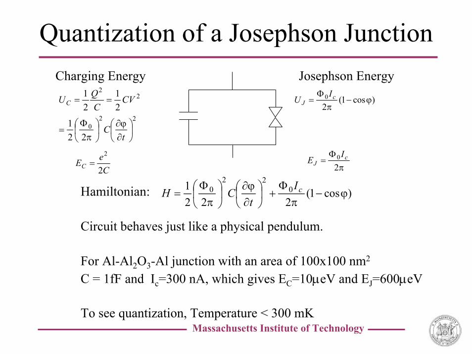
Quantization of a Josephson JunctionCharging Energy Josephson Energy

)cos1(20 ϕ−π

Φ= c

JI

U

220

22

221

21

21

∂ϕ∂

π

Φ=

==

tC

CVC

QUC

Hamiltonian:

Circuit behaves just like a physical pendulum.

For Al-Al2O3-Al junction with an area of 100x100 nm2

C = 1fF and Ic=300 nA, which gives EC=10µeV and EJ=600µeV

To see quantization, Temperature < 300 mK

)cos1(222

1 022

0 ϕ−π

Φ+

∂ϕ∂

π

Φ= cI

tCH

CeEC 2

2= π

Φ=

20 c

JI

E


Types of Superconducting Qubits

• Charge-state Qubits (voltage-controlled)– Cooper pair boxes

• Flux/Phase-state qubits (flux-current control)– Persistent Current Qubits– RF SQUID Qubits– Phase Qubits (single junction)

• Hybrid Charge-Phase Qubits


Charge-State Superconducting Qubit

TOP: “Electrical schematic”

BOTTOM: “Evidence of Rabi Oscillations”

Y. Nakamura, Yu A. Pashkin, and J.S. Tsai, Nature 398, 786 (1999).

Charge qubit a Cooper-pair box 3.0~/ CJ EE

φ

SQUID SQUID looploop

ProbeProbeBoxBoxGateGate

Tunnel Tunnel junctionjunction

SingleSingleCooperCooper--pair pair tunnelingtunneling ReservoirReservoir

Ωk 10~1R

ΩM 30~2R

Coherence up to ~ 5 ns, presently limited by background charge noise (dephasing) and by readout process (relaxation)

Y.Nakamura et al., Nature 398, 786 (1999).

Quantum Coherence in the Cooper-Pair Box Measured with an RF-SET

Schoelkopf Group, Yale University

2 e

• Superconducting charge qubit:the Cooper-pair box (CPB)

• Fast, single-charge readout:the RF single-electron transistor

• Quantum coherence of Cooper-pair box qubitobserved by CW microwave spectroscopy

RF-SETCPB

no µ-waves

40 GHz

<q>

Vg

• Transition frequency ~ 40 GHz: Qφ = ω10Tφ ~ 250 & Q1= ω10T1 > 105

• Ensemble decoherence time from linewidth: Tφ = 1 ns• Lifetime from time-resolved decay of photon peaks: T1= 1.6 µs

Funding: ARO/ARDA/NSA

Nextsteps:

• Operate @ charge-noise insensitive point to reduce decoherence• Perform time-gated, single-shot measurements


Our Persistent Current Qubit

• Depending on the direction of the current, state |0⟩and state |1⟩ will add a different magnetic field to the external magnet

• This difference is very small but can be distinguished by the extremely sensitive SQUID sensor


Quantum Computation with Superconducting Quantum DevicesT.P. Orlando, S. Lloyd, L. Levitov, J.E. Mooij - MIT

M. Tinkham – Harvard; M. Bocko, M. Feldman – U. of Rochesterin collaboration with K. Berggren, MIT Lincoln Laboratory

qubit&

readout

5 µm

Ic CJ

Ib

CsZ0qubit

ϕ2~ϕ1

~ • Persistent current qubit fabricated in Nb with submicron junctions

• Two states seen in measurement (thermal activations and energy levels)

1pF 1pF

0.45µm

1.1µm

0.55µm1.1µm

I- V-

I+ V+

Fabricationmodeling, and measurements


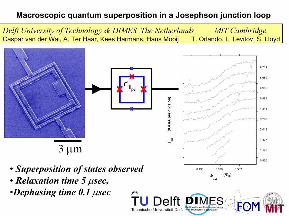
Macroscopic quantum superposition in a Josephson junction loop

Delft University of Technology & DIMES The Netherlands MIT CambridgeCaspar van der Wal, A. Ter Haar, Kees Harmans, Hans Mooij T. Orlando, L. Levitov, S. Lloyd

0.498 0.500 0.502

~

9.711

8.650

6.985

5.895

4.344

3.208

2.013

1.437

1.120

0.850

Ι SW(0

.4 n

A p

er d

ivis

ion)

Φext

(Φ0)

Ipc

3 µm

• Superposition of states observed• Relaxation time 5 µsec, •Dephasing time 0.1 µsec

TU DelftTechnische Universiteit Delft MIT

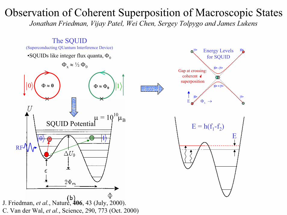
Observation of Coherent Superposition of Macroscopic StatesJonathan Friedman, Vijay Patel, Wei Chen, Sergey Tolpygo and James Lukens

|0>

|1>

|1>

|0>

|0> + |1>

|0> - |1>

Energy Levelsfor SQUID

Gap at crossing:coherent

superposition

Φx →E

The SQUID (Superconducting QUantum Interference Device)

•SQUIDs like integer flux quanta, Φ0

RF0 1

SQUID Potentialµ = 1010µB

×

>Φ ≈ 00

×

<Φ ≈ Φ0 1

J. Friedman, et al., Nature, 406, 43 (July, 2000). C. Van der Wal, et al., Science, 290, 773 (Oct. 2000)

E = h(f1-f2)E

Φx ≈ ½ Φ0

Quantum Computing with Superconducting DevicesF.C. Wellstood, C.J. Lobb, J.R. Anderson, and A.J. Dragt, Univ. of Md.

[email protected] / http://www.physics.umd.edu/sqc/

Objective Approach Status

• Measure energy levels and decoherence rates in single Josephson junctions and SQUIDs• Manipulate states of the systems• Perform 1-qubit operations• Design and test 2-qubit systems of junctions and SQUIDs

• Build Josephson junctions that are well isolated from measurement leads to achieve low dissipation and long coherence times at milliKelvin temperatures.• Measure macroscopic quantum tunneling, energy levels and decoherence rate.• Use microwaves to pump from |0> to |1> • Model SQUID qubits to guide experimental program.

• Built resistively isolated Al/AlOx/Al junctions and measured switching distributions with and without microwave excitation•Assembled SQUID detection scheme for measuring junctions and rf SQUIDs• Measured switching distributions for SQUID at mK temperatures, ∆Φ =10-3Φo

Objective

Recent Results from DURINT Quantum Computing ProjectSiyuan Han, Yang Yu et al., University of Kansas

Observation of Rabi oscillations in a Josephson Tunnel Junction

,150 A 5.8 pFc CI µ =0.30

0.25

0.20

0.15

0.10

0.05

0.00

P (

µs-1

)

20151050Time (µs)

2000

1000

0

P (

a.u.

)

2.01.51.00.50.0Time (µs)

Far off-resonance

0 1 101 ( )2 ϕγ γΓ = Γ + Γ + +

4.9decoherence time sµ>Generation and detection of RO in JJ

Quantum Computing with Current-Biased Josephson Junctions

John Martinis, S.W. Nam, J. Aumentado, C. Urbina; NIST Boulder

• Large area junctions - reliably fabricated using optical lithography

• Large capacitance allows coupling to many other qubits

Key Advantages:

VJJ = 1 mV

Measure |1> with ω12 :

ω12

0

12

VJJ = 0

U(δ)

qubit states

100 101 102 103 104

10-3

10-2

10-1

100

ω01 ω12 High Fidelity state preparation & measurement

|0> state prep : >99%|0> state meas : >99%

|1> state meas : >80%

Pro

b. in

sta

te |1

>

Power 01 µwave (cw) [arb. units]

theory

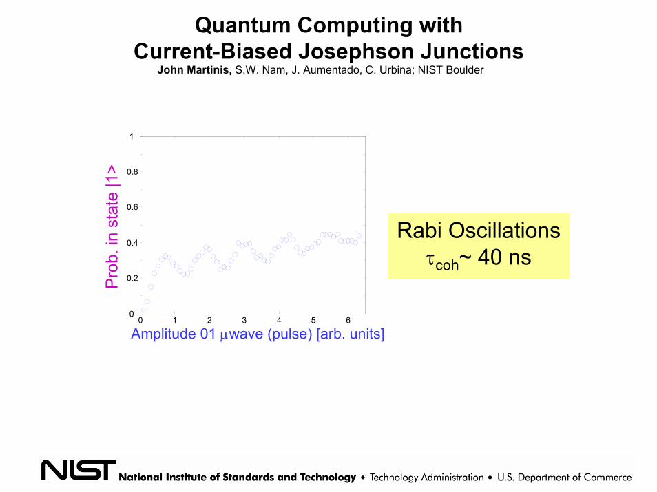
Quantum Computing with Current-Biased Josephson Junctions

John Martinis, S.W. Nam, J. Aumentado, C. Urbina; NIST Boulder

Pro

b. in

sta

te |1

>

Amplitude 01 µwave (pulse) [arb. units]

ω01 ω12

25 ns

0 1 2 3 4 5 60

0.2

0.4

0.6

0.8

1

Rabi Oscillations τcoh~ 40 ns

U WRITEPORT

READOUTPORT

Ib

Vi0

i1

ν01 TUNEPORT

largejunction

box

CHARGE-FLUXQUBIT

Quantronics GroupCEA-Saclay

France

M. Devoret (now at Yale)D. Esteve, C. UrbinaD. Vion, H. PothierP. Joyez, A. Cottet

Coherence time measuredby Ramsey fringes : 500nsQubit transition frequency:16.5 GHz; coherence qualityfactor: 25 000

0.0 0.1 0.2 0.3 0.4 0.5 0.6

30

35

40

45

sw

itchi

ng p

roba

bilit

y (%

)

time between pulses ∆t (µs)

RAMSEY FRINGES

νRF = 16409.50 MHz

0.0 0.1 0.2 0.3 0.4 0.5 0.6

30

35

40

45

sw

itchi

ng p

roba

bilit

y (%

)

time between pulses ∆t (µs)

Qϕ ~ 25000

∆t





c. Types of Qubits




3. Quantum Circuits




1. Charge qubits


3. Hybrid qubits


5. Outline of Class


Advantages of Superconductorsfor Quantum Computing

• Employs lithographic technology• Scalable to large circuits• Combined with on-chip, ultra-fast control electronics

– Microwave Oscillators – Single Flux Quantum classical electronics

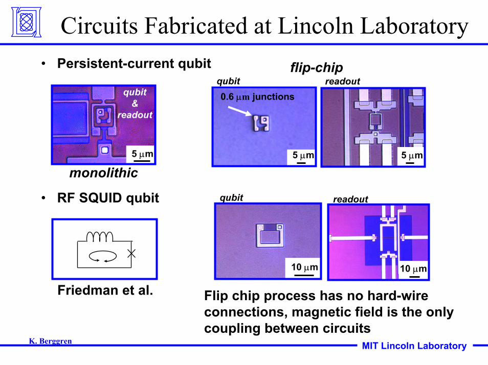
Circuits Fabricated at Lincoln Laboratory

monolithic

Flip chip process has no hard-wire connections, magnetic field is the only coupling between circuits

qubit&

readout

5 µm

Friedman et al.

5 µm5 µm

qubit

10 µm

readout

10 µm

qubit readoutflip-chip

0.6 µm junctionsqubit

• Persistent-current qubit

• RF SQUID qubit

MIT Lincoln LaboratoryK. Berggren

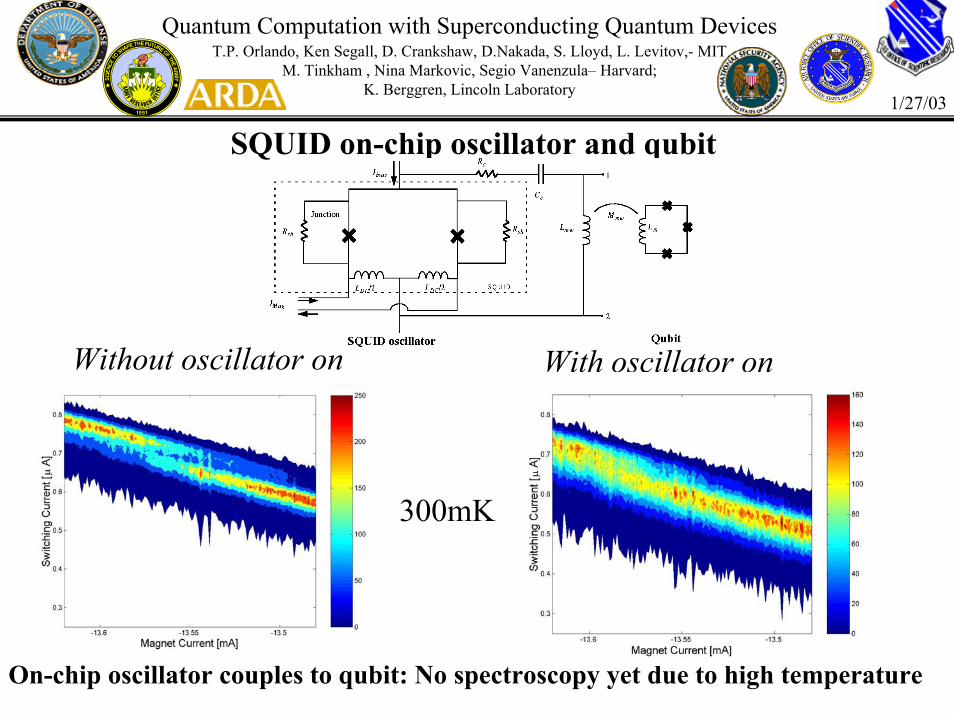
Quantum Computation with Superconducting Quantum DevicesT.P. Orlando, Ken Segall, D. Crankshaw, D.Nakada, S. Lloyd, L. Levitov,- MIT

M. Tinkham , Nina Markovic, Segio Vanenzula– Harvard;K. Berggren, Lincoln Laboratory

SQUID on-chip oscillator and qubit

On-chip oscillator couples to qubit: No spectroscopy yet due to high temperature

Without oscillator on With oscillator on

300mK

1/27/03

Feasibility of Superconductive Control Electronics Fabrication

Ope

ratin

g Sp

eed

(GH

z)

100 101 102 103 104 105 106

10

100

1

1000

qubitcontrol

SOURCESBerkeley

HitachiHypres

Lincoln LaboratoryNEC

Northrop-GrummanPhys.-Tech.-BundesanstaltState University of Moscow

U. of StonybrookTRW

others

Industry-Wide Demonstrations of Josephson Junction Circuits (at 4.2 K)

Number of Junctions

MIT Lincoln LaboratoryCompiled by K. Berggren

On-chip Control for an RF-SQUIDM.J. Feldman, M.F. Bocko, Univ. of Rochester

[email protected] www.ece.rochester.edu/~sde/


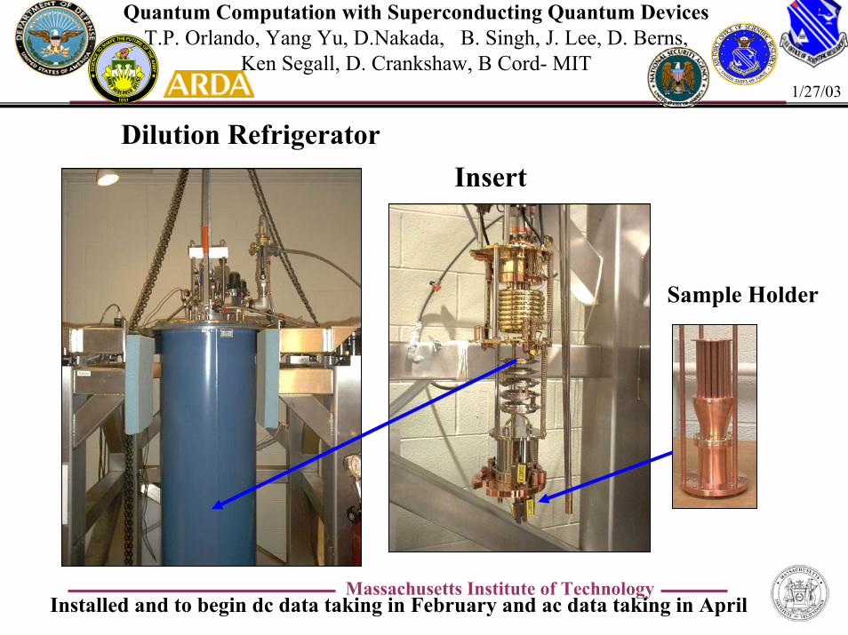
Quantum Computation with Superconducting Quantum DevicesT.P. Orlando, Yang Yu, D.Nakada, B. Singh, J. Lee, D. Berns,

Ken Segall, D. Crankshaw, B Cord- MIT1/27/03

Dilution RefrigeratorInsert

Sample Holder

Installed and to begin dc data taking in February and ac data taking in April





c. Types of Qubits




3. Quantum Circuits




1. Charge qubits


3. Hybrid qubits


5. Outline of Class


Outline of Class 6.9751. General Introduction and Overview of Quantized Circuits and Quantum Computing

2. Simple Quantized Circuits

a. Resistanceless circuits

b. Superconducting Josephson circuit elements

c. Energy storage in resistanceless circuits

d. Quantization of LC Oscillator Circuit

e. Quantization of Josephson junctions

3. Superconducting Quantum Circuits and Qubits

a. Charge and phase descriptions

b. Solutions to Schrödinger’s Equation for circuits

c. Single Josephson junction

d. Cooper pair box

e. Quantum RF SQUID

f. Persistent Current Qubits

g. Hybrid circuits


Outline of Class 6.9754. Quantum Computing

a. Two state system model

b. Qubits and coupled qubits

c. Manipulations of qubits

d. Fast control circuitry: SFQ electronics

5. Dissipation in Quantum Circuits

a. How to model a resistor

b. Decoherence: relaxation and dephasing

c. Spin-Boson model


Outline of Class 6.9756. Quantization of General Circuits

a. General network theory for classical circuits

i. Branch, nodal, and mesh formulations

ii. Inclusion of sources

iii. Lagrangian and Hamiltonian formulations

b. Network theory for quantum circuits

i. General canonical variables: charge, phase, and mesh currents

ii. Quantization without sources

iii. Transformations among canonical variables

c. Quantization with voltage and current sources

7. Assessment and Future Research in Quantum Circuits

Documents

Quantum Computing with Superconducting Devicesweb.mit.edu/6.763/www/SpecialTopics/ST03/notes/Lecture_1.pdf · 2003. 3. 5. · The Promise of a Quantum Computer A Quantum Computer