Embed Size (px)
Citation preview
Quantum Cryptography Without Basis Switching
Christian Weedbrook
B.Sc., University of Queensland, 2003.
A thesis submitted for the degree of
Bachelor of Science Honours in Physics
The Australian National University
October 2004

ii
iii
Listen, do you want to know a secret? Do you promise not to tell?
- John Lennon and Paul McCartney

iv
Declaration
This thesis is an account of research undertaken with the supervision of Dr Ping Koy Lam,
Dr Tim Ralph and Dr Warwick Bowen between February 2004 and October 2004. It is a
partial fulfilment of the requirements for the degree of a Bachelor of Science with Honours
in theoretical physics at the Australian National University, Canberra, Australia.
Except where acknowledged in the customary manner, the material presented in this
thesis is, to the best of my knowledge, original and has not been submitted in whole or
part for a degree in any university.
Christian Weedbrook
29th October 2004
v

vi
Acknowledgements
During the three years of residency, it was the relationships that got you
through.
- J.D., Scrubs
I have met a lot of people during my Honours year, and a lot of people to thank and
be thankful for. First I would like to thank my supervisors Ping Koy Lam, Tim Ralph,
Warwick Bowen and my “unofficial” supervisor Andrew Lance. Ping Koy, thank you for
your positive approach and enthusiasm. It was excellent having you as my supervisor,
as you have many ideas and the ability to know the best way to proceed. I would like
to thank you for my scholarship and also for organizing that I could do my Honours at
ANU, and to spend some time up at UQ. Tim, thanks for all your time and patience in
explaining things to me. Thanks for setting up the initial summer scholarship that lead
me to do Honours at ANU. Thank you for coming up with (and giving me) the original
idea that forms the basis of this thesis. Warwick, it was great working with you, you have
a great sense of humor that makes it more enjoyable to learn. Thank you for answering
all my questions and coming up with some great ideas. Andrew, it was great to have
been given the opportunity to work with you. You were available at any and all times to
patiently answer my questions, even when I was calling from Brisbane. Also thank you
Andrew and Warwick for initially getting me up to speed with the research. I cannot wait
to continue working with you all in the future.
Thanks to Craig Savage for all his help in making my particular arrangement possible
and for coordinating the Honours program. Next I would like to thank the head of the
Physics departments at ANU and UQ, Aiden Byrne and Halina Rubinsztein-Dunlop, for
allowing me to do my Honours program at ANU but also to spend time at UQ. I would
like to thank Aiden for organizing the Dean’s Faculty of Science scholarship. Thanks also
to Hans Bachor.
I have made a lot of friends during this year, both at the physics department and
college. I am grateful to be in such a great team as the quantum optics group, and
the friends I have made: Magnus Hsu, Andrew Lance, Thomas Symul, Katie Pilypas
(thanks for helping with my subject project), Vikram Sharma, Nicolai Grosse, and Vincent
Delaubert. I really appreciate of all your your company and help this year. I would like
to thank Amy Peng and Aditi Barthwal for their help and friendship too. Thanks also to
Max for sorting out all my computer problems while at ANU. A big part of any Honours
year is making sure that it does not become the only part of your year. And that is where
I want to thank my friends: Matthew Kinny, Chen Xu, Anna Smith, Hannah Woodall,
Will Young and Sharon Song, at John XXIII College, who provided a welcome distraction
from physics and who made my time in Canberra so much fun. I would also like to thank
the master at John XXIII College, Ken Evendon, for allowing me to stay at the college.
Thanks to all the other Honours students and various researchers who have helped me up
in Brisbane. Thanks to Aggie Branczyk for coming up with the polarizationsրւտց for my
vii
viii
thesis. And I would like to thank the quantum information people for various discussions,
particularly Andrew Doherty and Michael Nielsen.
In the last minute preparation of this thesis, I would like to thank Benedict Cusack
for helping me get it in on time. I appreciate everyone who proof read my thesis, and
corrected mistakes and made suggestions: Andrew, Ping Koy, Tim, Magnus, Vincent,
Thomas, Chen, Bobby Tonges and Alexandra Gramotnev. As the usual saying goes, if
there are still mistakes in the thesis, they are not totally to blame! This has been the best
year of my education so far and I look forward to continue working, and being with, the
same people over the next few years.
I would also like to thank my family in Brisbane. Finally and most importantly, I
would like to give my love and thanks to Alexandra, for all her love and support.
This thesis is dedicated to Alexandra.
Abstract
Quantum cryptography is one of the most interesting and popular fields in quantum in-
formation today. Its chief benefit lies in exploiting principles of quantum mechanics to
offer absolute security in the transmission of information. This thesis introduces a new
continuous variable quantum cryptographic protocol. The main difference between our
protocol and all previous ones, is the elimination of switching between measurement bases
- a step that was thought crucial in maintaining security. Our theoretical analysis shows
that by eliminating switching of measurement bases from the protocol, we still maintain
the required security, but also achieve significantly higher secret key rates than any other
known continuous variable quantum cryptographic protocol.
ix


Contents
Declaration v
Acknowledgements vii
Abstract ix
1 Introduction 3
1.1 Overview . . . . . . . . . . . . . . . . . . . . . . . . . . . . . . . . . . . . . 3
1.2 Thesis Structure . . . . . . . . . . . . . . . . . . . . . . . . . . . . . . . . . 5
1.3 Publication . . . . . . . . . . . . . . . . . . . . . . . . . . . . . . . . . . . . 5
2 Quantum Theory 7
2.1 The Uncertainty Principle . . . . . . . . . . . . . . . . . . . . . . . . . . . . 7
2.2 Phase Space Representation . . . . . . . . . . . . . . . . . . . . . . . . . . . 8
2.2.1 Coherent States . . . . . . . . . . . . . . . . . . . . . . . . . . . . . . 9
2.2.2 Squeezed State . . . . . . . . . . . . . . . . . . . . . . . . . . . . . . 10
2.3 Theoretical Concepts for Experiments . . . . . . . . . . . . . . . . . . . . . 10
2.3.1 Beam Splitters and Vacuum Noise . . . . . . . . . . . . . . . . . . . 11
2.3.2 Detecting Quantum States of Light . . . . . . . . . . . . . . . . . . . 11
2.4 Conclusion . . . . . . . . . . . . . . . . . . . . . . . . . . . . . . . . . . . . 13
3 Classical Cryptography 15
3.1 Introduction . . . . . . . . . . . . . . . . . . . . . . . . . . . . . . . . . . . . 15
3.2 A Brief History of Cryptography . . . . . . . . . . . . . . . . . . . . . . . . 16
3.3 The Distribution of Keys . . . . . . . . . . . . . . . . . . . . . . . . . . . . 17
3.3.1 Private Key Distribution . . . . . . . . . . . . . . . . . . . . . . . . 17
3.3.2 Public Key Distribution . . . . . . . . . . . . . . . . . . . . . . . . . 18
3.4 Shor’s Algorithm . . . . . . . . . . . . . . . . . . . . . . . . . . . . . . . . . 19
3.5 Conclusion . . . . . . . . . . . . . . . . . . . . . . . . . . . . . . . . . . . . 19
4 Quantum Cryptography 21
4.1 Introduction . . . . . . . . . . . . . . . . . . . . . . . . . . . . . . . . . . . . 21
4.2 Quantum Money . . . . . . . . . . . . . . . . . . . . . . . . . . . . . . . . . 21
4.2.1 The No Cloning Theorem . . . . . . . . . . . . . . . . . . . . . . . . 22
4.3 Discrete Quantum Cryptography . . . . . . . . . . . . . . . . . . . . . . . . 23
4.3.1 The BB84 Protocol . . . . . . . . . . . . . . . . . . . . . . . . . . . . 23
4.4 Continuous Variable Quantum Cryptography . . . . . . . . . . . . . . . . . 25
4.4.1 Steps of the Protocol . . . . . . . . . . . . . . . . . . . . . . . . . . . 26
4.4.2 Direct and Reverse Reconciliation Protocols . . . . . . . . . . . . . . 26
4.4.3 Eavesdropping . . . . . . . . . . . . . . . . . . . . . . . . . . . . . . 27
4.5 Key Distillation and Privacy Amplification . . . . . . . . . . . . . . . . . . 28
4.6 Experimental Quantum Cryptography . . . . . . . . . . . . . . . . . . . . . 28
xi
xii Contents
4.7 Conclusion . . . . . . . . . . . . . . . . . . . . . . . . . . . . . . . . . . . . 29
5 Quantum Cryptography Without Basis Switching 31
5.1 Introduction . . . . . . . . . . . . . . . . . . . . . . . . . . . . . . . . . . . . 31
5.2 The SQM Protocol . . . . . . . . . . . . . . . . . . . . . . . . . . . . . . . . 33
5.2.1 Steps of the SQM Protocol . . . . . . . . . . . . . . . . . . . . . . . 33
5.2.2 Conditional Variance . . . . . . . . . . . . . . . . . . . . . . . . . . . 34
5.2.3 Alice’s Conditional Variance . . . . . . . . . . . . . . . . . . . . . . . 35
5.2.4 Eve’s Conditional Variance . . . . . . . . . . . . . . . . . . . . . . . 36
5.2.5 Secret Key Rate . . . . . . . . . . . . . . . . . . . . . . . . . . . . . 36
5.3 Eavesdropping Attack . . . . . . . . . . . . . . . . . . . . . . . . . . . . . . 39
5.3.1 Feed Forward Protocol . . . . . . . . . . . . . . . . . . . . . . . . . . 39
5.3.2 Conditional Variances and Information Rates . . . . . . . . . . . . . 40
5.4 Conclusion . . . . . . . . . . . . . . . . . . . . . . . . . . . . . . . . . . . . 42
6 Conclusions and Future Work 43
6.1 Summary . . . . . . . . . . . . . . . . . . . . . . . . . . . . . . . . . . . . . 43
6.2 Future Work . . . . . . . . . . . . . . . . . . . . . . . . . . . . . . . . . . . 43
6.2.1 The SQM Protocol using Postselection . . . . . . . . . . . . . . . . . 43
6.2.2 Other Quantum Cryptographic Proposals . . . . . . . . . . . . . . . 44
6.2.3 The Accessible Information of Quantum States . . . . . . . . . . . . 44
6.3 Conclusion . . . . . . . . . . . . . . . . . . . . . . . . . . . . . . . . . . . . 45
A Matlab Code for Feed Forward Optimization 47
Bibliography 49
Index 53

List of Figures
2.1 Phase space or “ball and stick” representation of the light field. . . . . . . . 9
2.2 Three types of phase space representations. . . . . . . . . . . . . . . . . . . 10
2.3 Schematic diagram of a beam splitter . . . . . . . . . . . . . . . . . . . . . 11
2.4 Schematic diagram of direct detection. . . . . . . . . . . . . . . . . . . . . . 12
2.5 Schematic diagram of homodyne detection. . . . . . . . . . . . . . . . . . . 13
3.1 The process of cryptography . . . . . . . . . . . . . . . . . . . . . . . . . . . 16
3.2 The one-time pad . . . . . . . . . . . . . . . . . . . . . . . . . . . . . . . . . 18
4.1 Example of quantum money . . . . . . . . . . . . . . . . . . . . . . . . . . . 22
4.2 Discrete quantum cryptography or BB84 protocol . . . . . . . . . . . . . . . 25
4.3 The continuous variable quantum cryptography protocol . . . . . . . . . . 27
4.4 Sliced reconciliation protocol . . . . . . . . . . . . . . . . . . . . . . . . . . 29
5.1 Schematics of the SQM protocol . . . . . . . . . . . . . . . . . . . . . . . . 32
5.2 Contour plot of the information rate for the SQM protocol . . . . . . . . . . 34
5.3 Net information rates for the simultaneous and single quadrature schemes . 37
5.4 Feed forward schematic of the SQM protocol . . . . . . . . . . . . . . . . . 40
5.5 Information rates for the simultaneous and single quadrature schemes . . . 41
1

2 LIST OF FIGURES
Chapter 1
Introduction
O-Ren Ishii: You didn’t think it was gonna be that easy, did you?
The Bride: You know, for a second there, yeah, I kinda did.
- KILL BILL Vol.1
1.1 Overview
The desire to communicate in private has always been apart of human civilization. Al-
though its origins are unknown, it would almost certainly have started not long after the
beginning of literacy. The art of communicating in secret, between a sender and receiver,
is known as cryptography [1]. It has a long and fascinating history, full of exciting and
interesting stories: the assassination of a Queen, the world of espionage, the secret hid-
ing and disguising of messages, Enigma machines and much more [2, 1]. Cryptography
usually consists of encrypting a message with a secret key. As a result the message is
then scrambled and is only able to be read by the receiver, who also has a key. For this
reason, the key is kept private. However, cryptography was changed in the 1970’s, when
it was discovered that you could publicly distribute your key and yet still maintain secure
communications. An example of this public key distribution is the RSA code, which forms
the basis of all of today’s crypto-communication systems. Since the very beginning, there
has been a back and forth struggle between the code-maker and code-breaker to remain
dominate. However, in 1984 a new advancement in cryptography might have ended the
struggle for good, in favor of the code-maker. A new theory called quantum mechanics is
the reason why.
Since its beginnings in the early twentieth century, quantum mechanics [3] has devel-
oped a successful theoretical framework for the world around us. It is a theory based on
the atomic or microscopic world, and is probabilistic in nature. Quantum optics [4] is a
branch of quantum theory, that deals with the description and controlling of optical light
fields. It illustrates the differences between our everyday “classical” world and the weird
and wonderful quantum world, by revealing such non-classical features as squeezing [5, 6]
and entanglement [7]. During the last few decades, quantum physics, along with quantum
optics, have come together to form new ways of processing information. This is known as
quantum information [8].
Quantum information is currently receiving enormous interest and success in both
theoretical and experimental physics. It is a combination of quantum physics with com-
puter science and mathematics, with a goal of providing more efficient and secure ways of
3
4 Introduction
transmitting and processing information. Quantum information theory has lead to such
exciting and diverse topics as teleportation [9], quantum computation [10, 11], quantum
error correction [12], dense coding [13] and quantum search algorithms [14]. These appli-
cations of quantum mechanics were originally developed using discrete variables. These
discrete systems deal with the manipulation of quantum bits (qubits) or single photon
states. However there has been a move towards continuous variables, which are easier
to generate and offer higher bandwidths and higher quantum efficiency production in the
measuring of quantum states. This has lead to continuous variable quantum information
theory [15]. The main incentive for this transfer, is due to more practical considerations in
quantum information protocols. The detecting of discrete single photons has an efficiency
of about 60%, whereas the continuous systems have an efficiency of near unity. This thesis
will be concerned with continuous variable systems and in particular, continuous variable
quantum cryptography.
Quantum cryptography [16] is the science of sending secret messages using properties
of quantum mechanics. This property is namely the inability to simultaneously measure
two non-commuting observables perfectly. As it is these observables that the information is
encoded onto, any eavesdropper will ultimately disturb the quantum system and therefore
add additional noise. Consequently a sender and receiver are able to generate a correlated
secure key; provided this disturbance or noise is below a certain allowable level. Quantum
cryptography could have been invented as soon as quantum mechanics was discovered and
understood in the first few decades of the 20th century. However it was only revealed in
1984 [17] after an unpublished paper in 1970 [18]. Now quantum cryptography offers the
possibility of 100% security against any eavesdropper. Finally ending the battle between
the code-maker and the code-breaker. The first version of quantum cryptography, or
quantum key distribution (as it is also known), was using discrete photon polarizations.
In 1999 a continuous variable version was formed which offered a number of benefits
over the discrete regime [19]. All forms of quantum cryptography had what seemed an
inherent step in their protocols. The switching of measurement bases. For over 20 years
now, switching has appeared in all quantum key distribution protocols and it was thought
that the security of these protocols was due to this switching. This leads to the two main
aims of this thesis:
• Do quantum cryptographic protocols require switching?
Switching refers to a technique used by the receiver, to randomly switch the mea-
surement bases. It has long been a part of both the discrete and continuous variable
schemes of quantum cryptography. It was thought that switching offers the neces-
sary condition for security in these protocols. We will investigate whether switching
is absolutely necessary and if we can create a new continuous variable quantum cryp-
tography protocol that resists the need to randomly switch between measurement
bases.
• If no, then how does it compare to previous protocols?
The process of switching in the continuous variable regimes limits the bandwidth
in the cryptographic protocols. Therefore the elimination of switching would offer
practical advantages: simplicity and higher bandwidths. In fact, our results [20] in
Chapter 5 will show that switching, which has existed for over two decades now,
is no longer necessary. The protocol that we have developed, known as the SQM
protocol, is also applicable to previous coherent state continuous variable quantum
cryptographic protocols.
§1.2 Thesis Structure 5
1.2 Thesis Structure
This thesis consists of five main chapters. Chapter 2 introduces the major theoretical
concepts that will be used in this thesis. These concepts deal with the foundations of
quantum mechanics and the fundamentals of quantum optics. Chapter 3 introduces clas-
sical cryptography: its history, the idea of key distributions (both private and public)
and how an application of quantum theory, in the form of quantum computers, provides
insecurities in today’s classical encryption protocols. Chapter 4 introduces quantum cryp-
tography and begins with its origins in quantum money. We then discuss the two main
forms of quantum cryptography: discrete and continuous. Key distillation and privacy
amplification are then introduced with a final comment on the experimental versions of
quantum cryptography. Chapter 5 consists of the original research that was undertaken
in this thesis and introduces our new quantum cryptographic protocol. Chapter 6 ends
with concluding remarks along with the future prospects of both quantum cryptography
and quantum information in general.
1.3 Publication
A publication has resulted from the work that was carried out in this thesis. The original
research, which appears in Chapter 5, has been published in the following journal article:
• Quantum Cryptography Without Switching,
Christian Weedbrook, Andrew Lance, Warwick Bowen, Thomas Symul, Tim Ralph
and Ping Koy Lam,
Physical Review Letters 93, 170504 (2004).
6 Introduction
Chapter 2
Quantum Theory
A newspaper can be read and you don’t hurt it by reading it. For really small
things, the process of observing them disturbs them.
- Charles Bennett
Dr. Emmett Brown: 1.21 gigawatts? 1.21 gigawatts? Great Scott!
Marty McFly: What the hell is a gigawatt?
- Back to the Future
This chapter introduces a theoretical framework that will be used throughout this the-
sis. We introduce such fundamental concepts as the uncertainty principle, phase space
representation and detecting quantum states of light.
2.1 The Uncertainty Principle
We cannot know, as a matter of principle, the present in all its details.
- Werner Heisenberg
Quantum mechanics is one of the most successful theories in the history of science. It
is a probabilistic theorem, which as a result, often deals with uncertainties and statistics.
One concept, the uncertainty relation, illustrates this view of quantum mechanics and
can be derived using commutators. In quantum theory, the commutator of two arbitrary
observables1, A and B, is a mathematical operation given by
[A, B] = AB − BA (2.1)
The operators A and B are said to commute when [A, B] = 0 and are non-commuting
when [A, B] 6= 0. One physical interpretation of two observables commuting is that we
can determine their values exactly, i.e. without any uncertainty. However if they are
non-commuting then it is impossible to determine them both simultaneously, without
1An observable corresponds to the eigenvalue of its operator. It is hermitian since it has real expectationvalues.
7
8 Quantum Theory
any uncertainty or error. One such example is say, [A, B] = 2iC, where C is a complex
constant. Then the product of these uncertainties is given by
∆A∆B ≥ 〈|C|〉 (2.2)
where ∆A and ∆B are the uncertainties. Equation (2.2) is known as the Heisenberg
uncertainty principle . By taking the square of these uncertainties or standard deviations
given in Eq. (2.2), we end up with
VAVB ≥ C2 (2.3)
where VA = 〈(∆A)2〉 and VB = 〈(∆B)2〉. The standard deviation for any arbitrary
operator D is defined as
∆D =√
〈D2〉 − 〈D〉2 (2.4)
The uncertainty relation is an important consequence of quantum mechanics and can be
used, along with the non-Hermitian boson annihilation and creation operators, to give an
understanding of a quantum system. The annihilation operator a and creation operator
a† are mathematical functions that can describe the light field as either a function of time
a(t) or frequency a(ω). The operators for this thesis are assumed to be a function of time.
The boson commutator relation of these two field operators is
[a, a†] = 1 (2.5)
where a = 12(X+ + iX−) [5]. We can define a new set of operators, known as quadratures,
from the annihilation and creation operators
X+ = a† + a (2.6)
X− = i(a† − a) (2.7)
Here X+ and X− correspond to the amplitude and phase of an electric field, respectively,
and are analogous to position and momentum in classical physics. The commutator of
these quadratures is given by
[X+, X−] = 2i (2.8)
Using Eq. (2.2), this leads to uncertainty and variance relations of
∆X+∆X− ≥ 1 (2.9)
V +V − ≥ 1 (2.10)
This shows us that we cannot simultaneously measure the amplitude and phase quadra-
tures precisely or without assuming some sort of penalty. Equation (2.10) has a lower
limit of 1. This lower bound is known as the quantum noise limit or the shot noise limit.
2.2 Phase Space Representation
The phase space gives a two dimensional representation of the two orthogonal quadratures,
X+ and X−, that describe a continuous variable light field. This diagrammatic scheme
§2.2 Phase Space Representation 9
X+
X_
(X+)2
(X_)2< >
><
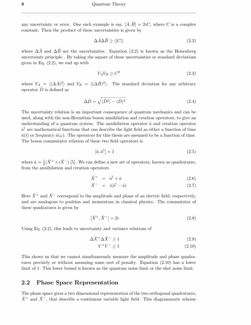
Figure 2.1: Phase space or “ball and stick” representation of the light field.
can also be viewed as a “ball and stick” picture (see Fig. 2.1). The length of the stick is the
classical field amplitude and the ball represents the quantum fluctuations or uncertainty
in both quadratures. So when the quantum uncertainty is much less than the classical
amplitude and the average fluctuations are zero, we can linearize the field operators using
a = α + δa (2.11)
a† = α∗ + δa† (2.12)
where α is a c-number representing the steady state or amplitude and δa are the quantum
fluctuations (so we are simply defining δa = a − 〈a〉). Thus in the phase space repre-
sentation the stick is the steady state or classical amplitude and the ball is the quantum
fluctuations. The diameter of the ball is regarded as the variance of each quadrature. Two
common states of light that can be represented on phase space are the coherent state and
the squeezed state.
2.2.1 Coherent States
A coherent state is the most quasi-classical of all quantum states. This is because it is
a minimum uncertainty state that lower bounds the inequality given in Eq. (2.9), i.e.
V +V − = 1. Figure (2.1) shows a coherent state as represented by a phase space diagram.
A coherent state |α〉 can be written as a sum of number or Fock states |n〉
|α〉 = e−|α2|2
∞∑
n
αn
√n!|n〉 (2.13)
where all possible Fock states can be generated by repeatedly applying the annihilation
operator on a vacuum state |0〉. This is defined mathematically as
|n〉 =(a†)n
√n!
|0〉 (2.14)
A coherent state has the following properties
a|α〉 = α|α〉 (2.15)
10 Quantum Theory
|α〉 = D|0〉 (2.16)
where D = exp(αa†−α∗a) is called the displacement operator. Therefore the coherent state
is the eigenstate of the annihilation operator and is obtained by acting the displacement
operator on the vacuum state. A type of coherent state that is worth mentioning is the
vacuum state |0〉. It has the same quantum fluctuations as a coherent state but with an
average number of photons equal to zero. So on the “ball and stick” picture it would be a
ball centered at the origin with no stick (see Fig. 2.2). One place that the vacuum state
enters into our analysis is through a beam splitter (see below).
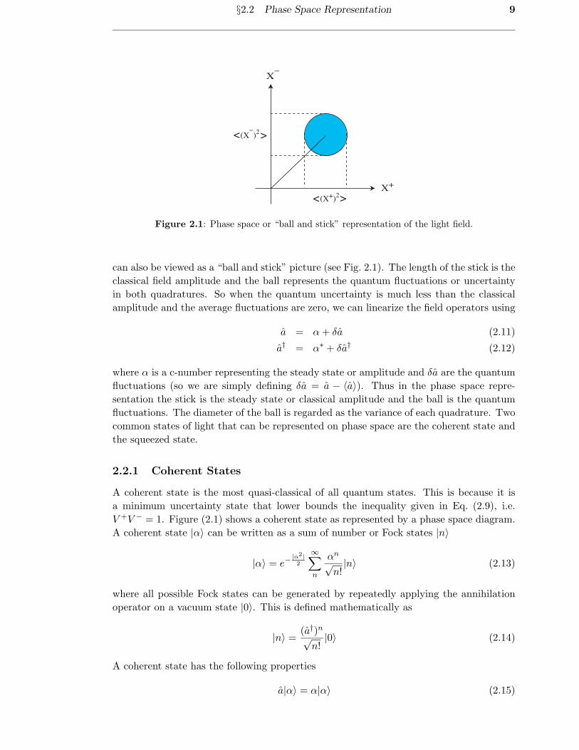
2.2.2 Squeezed State
Squeezing is when one of the uncertainties in Eq. (2.9) is reduced (“squeezed”) below the
quantum noise limit (Fig. 2.2 shows a squeezed state in phase space). In order for this
inequality to still hold, the other uncertainty is increased. Amplitude squeezing is when
V + < 1 and V − > 1 and phase squeezing is when V − < 1 and V + > 1. Perfect squeezing
in the amplitude quadrature occurs when V + → 0 resulting in the phase quadrature
V − → ∞. Anti-squeezing results when one of the quadratures is greater than 1. The
amount of squeezing is characterized by the squeezing parameter s±, where 0 ≤ s± ≤ 1.
Understanding that the uncertainty relation between the squeezing parameter and the
variable must hold, leads to
s± ≥ 1
V∓ (2.17)
which comes from the fact that V +V − = 1. The creation of squeezed light [21, 22] can
be useful in the generation of entanglement and such applications as gravitational wave
detection and quantum cryptography.
X_
(X+)2
(X_)2
(a)
< >
><X+ X+
X_
(X+)2
(X_)2
(b)
>
>
<
<
(c)
X+
X_
Figure 2.2: Three types of phase space representations. (a) Coherent State (b) A squeezed state
(amplitude squeezed) (c) Vacuum state.
2.3 Theoretical Concepts for Experiments
A number of the theoretical concepts in this thesis are based on experimental techniques,
including the use of beam splitters (and the vacuum noise associated with it) and the
measuring processes that are needed to understand and analyze the incoming light field.

§2.3 Theoretical Concepts for Experiments 11
2.3.1 Beam Splitters and Vacuum Noise
Dr. Egon Spengler : Wait! Wait! There’s something I forgot to tell you.
Dr. Peter Venkman : What?
Dr. Egon Spengler : Don’t cross the streams.
Dr. Peter Venkman : Why not?
Dr. Egon Spengler : Trust me. It would be bad.
- Ghostbusters
A beam splitter is one of the most commonly used tools in applications relating to quantum
information. It is an optical device that splits an incoming light beam into two beams:
one reflected beam and one transmitted beam. One feature of a beam splitter is the
coupling in of vacuum noise with the incoming light. This influx of vacuum noise is a
quantum mechanical feature that is necessary in order to preserve, among other things,
the uncertainty principle and the bosonic commutator relations. In Fig. 2.3, an incoming
light beam, characterized by the boson field operator a, hits a beam splitter in which
vacuum noise b has entered. The two output operators are given by the following beam
splitter equations
d =√
η a +√
1 − η b (2.18)
c =√
1 − η a −√η b (2.19)
where η is the transmission coefficient that ranges in value from 0 to 1: with 0 indicating
a
b
c
dη
Figure 2.3: Schematic diagram of a beam splitter
zero transmission and 100% refection and with 1 signifying the complement. It is important
to note that when we take the variance of Eq. (2.18), the variance of the vacuum noise
will be normalized to unity, i.e. Vb = 〈(b)2〉 = 1.
2.3.2 Detecting Quantum States of Light
The theory of measurement processes is an important part of any analysis involving quan-
tum theory. We have already introduced variances and quadratures, which are all im-
portant theoretical concepts. But how do we go about measuring them? This process
consists of a detector that transforms the incoming beam of light into a photocurrent
which is transformed into statistical data via a spectrum analyzer. Two such processes
include direct detection and standard homodyne detection.
12 Quantum Theory
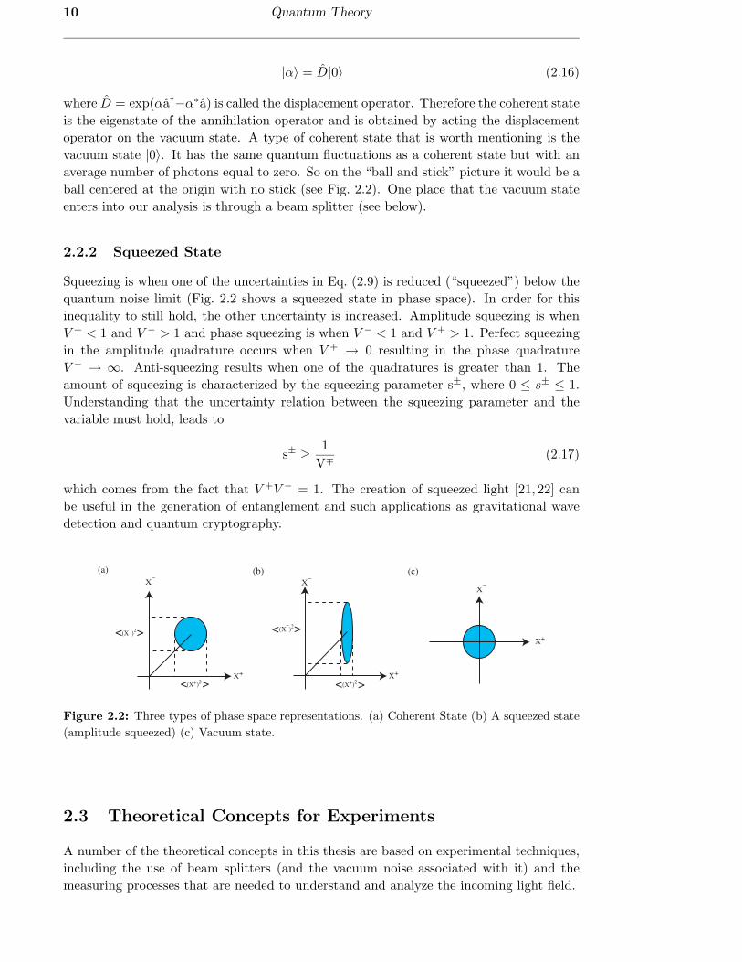
Direct Detection
Direct detection (see Fig. 2.4) is a simple optical measurement whose photocurrent I(t) is
proportional to the intensity of the light field
I(t) ∝ |α|2 + α δX+(t) (2.20)
where α is the classical amplitude. This shows us that by measuring this direct detec-
tion photocurrent we can, in principle, measure the amplitude quadrature ∆X+(t) to an
arbitrary precise value. The phase quadrature measurement can not be obtained by this
method. This is due to the destruction of the phase as a result of the rapid oscillation
of the electric field with respect to the electric current. The phase quadrature can be
measured using standard homodyne detection.
SA
I(t)a Detector
Figure 2.4: Schematic diagram of direct detection. An incoming light field, described by the
operator a, hits a detector. The light is then transformed into a photocurrent I(t), which can be
studied by a spectrum analyzer.
Standard Homodyne Detection
A homodyne detector is an experimental tool used to measure either the amplitude or
phase quadratures of a light field (see Fig. 2.5). Self-homodyning is when the incoming
light is interacted with the vacuum noise that enters into the other unused port of the
beam splitter. We can then take the sum (difference) of the photocurrents to measure
the amplitude of the incoming signal beam (vacuum noise). Homodyning with a local
oscillator2 (LO) is a form of optical mixing that allows us to determine the phase quadra-
ture. The local oscillator is a bright light (large amplitude) of a much higher photon
number than the incoming signal (sig). By taking the sum (s) and difference (d) of the
photocurrents we arrive at
I(t)s ∝ βδX+LO (2.21)
I(t)d ∝ βδX(θ+π/2) (2.22)
where β is the steady state of the local oscillator, θ is the phase between the local oscillator
and signal beam, and we have only included the quantum fluctuations. From this we see
2The phase of something is only known with respect to something else. Thus a local oscillator is abright beam of light with a known phase that acts like a clock or reference point in which other beams canthen be compared to.
§2.4 Conclusion 13
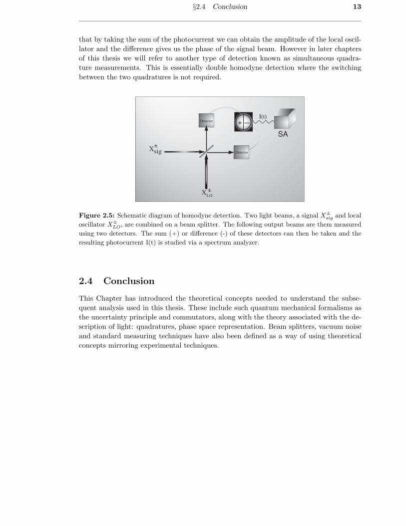
that by taking the sum of the photocurrent we can obtain the amplitude of the local oscil-
lator and the difference gives us the phase of the signal beam. However in later chapters
of this thesis we will refer to another type of detection known as simultaneous quadra-
ture measurements. This is essentially double homodyne detection where the switching
between the two quadratures is not required.
+ _
Xsig
XLO
SA
+_
+_
I(t)Detector
Detector
Figure 2.5: Schematic diagram of homodyne detection. Two light beams, a signal X±
sig and local
oscillator X±
LO, are combined on a beam splitter. The following output beams are them measured
using two detectors. The sum (+) or difference (-) of these detectors can then be taken and the
resulting photocurrent I(t) is studied via a spectrum analyzer.
2.4 Conclusion
This Chapter has introduced the theoretical concepts needed to understand the subse-
quent analysis used in this thesis. These include such quantum mechanical formalisms as
the uncertainty principle and commutators, along with the theory associated with the de-
scription of light: quadratures, phase space representation. Beam splitters, vacuum noise
and standard measuring techniques have also been defined as a way of using theoretical
concepts mirroring experimental techniques.

14 Quantum Theory
Chapter 3
Classical Cryptography
Joey: Hey Chandler, when you see Frankie tell him that Joey says hi. He’ll
know what it means.
Chandler: Gee, I don’t know. Do you think he’ll be able to crack your code?
- Friends
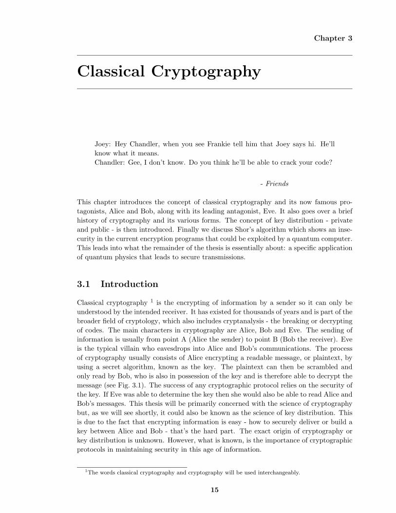
This chapter introduces the concept of classical cryptography and its now famous pro-
tagonists, Alice and Bob, along with its leading antagonist, Eve. It also goes over a brief
history of cryptography and its various forms. The concept of key distribution - private
and public - is then introduced. Finally we discuss Shor’s algorithm which shows an inse-
curity in the current encryption programs that could be exploited by a quantum computer.
This leads into what the remainder of the thesis is essentially about: a specific application
of quantum physics that leads to secure transmissions.
3.1 Introduction
Classical cryptography 1 is the encrypting of information by a sender so it can only be
understood by the intended receiver. It has existed for thousands of years and is part of the
broader field of cryptology, which also includes cryptanalysis - the breaking or decrypting
of codes. The main characters in cryptography are Alice, Bob and Eve. The sending of
information is usually from point A (Alice the sender) to point B (Bob the receiver). Eve
is the typical villain who eavesdrops into Alice and Bob’s communications. The process
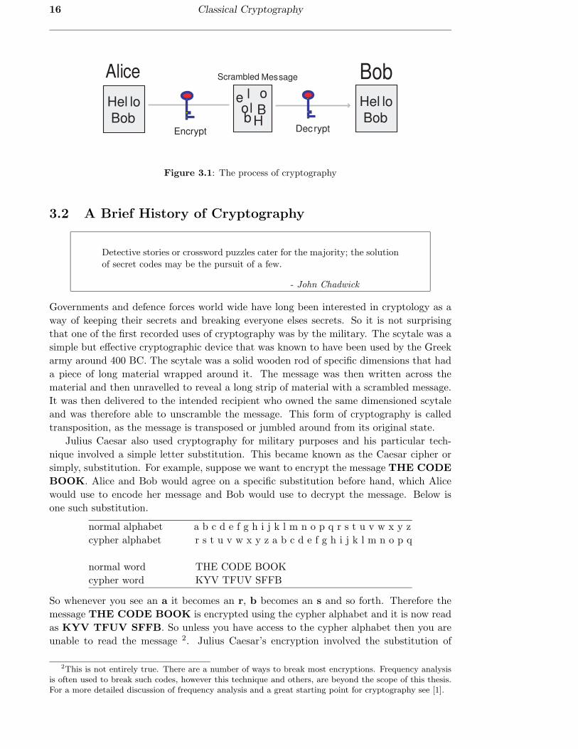
of cryptography usually consists of Alice encrypting a readable message, or plaintext, by
using a secret algorithm, known as the key. The plaintext can then be scrambled and
only read by Bob, who is also in possession of the key and is therefore able to decrypt the
message (see Fig. 3.1). The success of any cryptographic protocol relies on the security of
the key. If Eve was able to determine the key then she would also be able to read Alice and
Bob’s messages. This thesis will be primarily concerned with the science of cryptography
but, as we will see shortly, it could also be known as the science of key distribution. This
is due to the fact that encrypting information is easy - how to securely deliver or build a
key between Alice and Bob - that’s the hard part. The exact origin of cryptography or
key distribution is unknown. However, what is known, is the importance of cryptographic
protocols in maintaining security in this age of information.
1The words classical cryptography and cryptography will be used interchangeably.
15
16 Classical Cryptography
Alice Bob
Encrypt Dec rypt
Scrambled
Hel lo Bob
Hel lo BobH
ell o
Bob
Mes sage
Figure 3.1: The process of cryptography
3.2 A Brief History of Cryptography
Detective stories or crossword puzzles cater for the majority; the solution
of secret codes may be the pursuit of a few.
- John Chadwick
Governments and defence forces world wide have long been interested in cryptology as a
way of keeping their secrets and breaking everyone elses secrets. So it is not surprising
that one of the first recorded uses of cryptography was by the military. The scytale was a
simple but effective cryptographic device that was known to have been used by the Greek
army around 400 BC. The scytale was a solid wooden rod of specific dimensions that had
a piece of long material wrapped around it. The message was then written across the
material and then unravelled to reveal a long strip of material with a scrambled message.
It was then delivered to the intended recipient who owned the same dimensioned scytale
and was therefore able to unscramble the message. This form of cryptography is called
transposition, as the message is transposed or jumbled around from its original state.
Julius Caesar also used cryptography for military purposes and his particular tech-
nique involved a simple letter substitution. This became known as the Caesar cipher or
simply, substitution. For example, suppose we want to encrypt the message THE CODE
BOOK. Alice and Bob would agree on a specific substitution before hand, which Alice
would use to encode her message and Bob would use to decrypt the message. Below is
one such substitution.
normal alphabet a b c d e f g h i j k l m n o p q r s t u v w x y z
cypher alphabet r s t u v w x y z a b c d e f g h i j k l m n o p q
normal word THE CODE BOOK
cypher word KYV TFUV SFFB
So whenever you see an a it becomes an r, b becomes an s and so forth. Therefore the
message THE CODE BOOK is encrypted using the cypher alphabet and it is now read
as KYV TFUV SFFB. So unless you have access to the cypher alphabet then you are
unable to read the message 2. Julius Caesar’s encryption involved the substitution of
2This is not entirely true. There are a number of ways to break most encryptions. Frequency analysisis often used to break such codes, however this technique and others, are beyond the scope of this thesis.For a more detailed discussion of frequency analysis and a great starting point for cryptography see [1].
§3.3 The Distribution of Keys 17
Roman letters with Greek letters, which was enough to ensure his message did not fall
into his enemy’s hands.
Another form of cryptography is steganography. This form of security involved the
physical hiding of a message from the enemy. Ancient cultures would shave a messenger’s
head and write a note on it. They would then wait for the hair to grow back and send
him to the receiver who would again shave his head to reveal the message. Clearly not
the most time saving of all cryptographic protocols! Another example of steganography
occurred during World War II. A secret document would be shrunk to the size of a full
stop and then hidden over the top of a full stop on a typed page. A lot of encryption
techniques would inevitably use a combination of say, substitution and transposition, in
order to maximize the message’s security. The scytale could also used as a steganographic
device, sometimes being disguised as a belt around the messenger. The document that
was shrunk to the size of a full stop could also have been encrypted before it was reduced,
by using, for example, transposition or substitution. For a more detailed experience of the
history of cryptography see [2, 1].
3.3 The Distribution of Keys
How’s that...the key’s run off.
- Jack Sparrow, Pirates of the Caribbean
The secure delivery of a key - or key distribution as it is known - is at the heart of what
cryptography is essentially about. There are two main types of key distribution: private
and public.
3.3.1 Private Key Distribution
Private key distribution is where the security of a protocol is dependent on the safe delivery
of the key between Alice and Bob. During the Second World War, the German military
used the famous Enigma machines. The Enigma was a complex encryption device that
relied on the daily distribution of code books (the key) in order to ensure security. Because
these keys could only be entrusted to the intended recipient, it is an example of private
key distribution. Another famous protocol that relied on the distribution of a private key
was the Vernam cipher or the “one-time pad” as it is also known.
The One-Time Pad
The one-time pad was developed in 1917 by an American engineer Gilbert Vernam, and
was significantly used during the latter stages of World War 1. It is the only known
classical cypher that is proven to be 100% secure 3. The one-time pad cypher, as its name
suggests, can only be used once 4 and the randomness is the key to its security. This is
because if the key was reused a number of times, a potential code breaker could build
up patterns from the rehashed key. We will see later on that the one-time pad is also an
important tool used in quantum cryptography. Figure 3.2 gives a simple illustration of
3Its complete security was actually only proved 10 years after World War 1 by Charles Shannon.4The word pad comes from the fact that spies used to quickly write something down on a note book or
pad and then tear it off.
18 Classical Cryptography
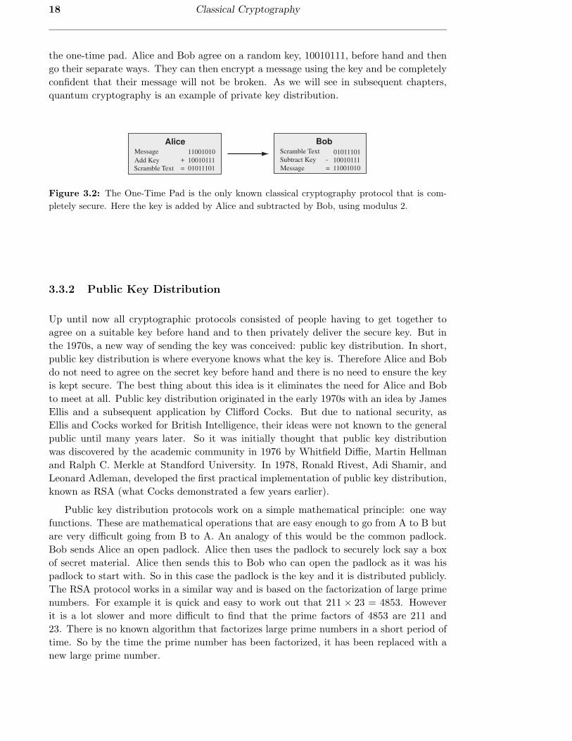
the one-time pad. Alice and Bob agree on a random key, 10010111, before hand and then
go their separate ways. They can then encrypt a message using the key and be completely
confident that their message will not be broken. As we will see in subsequent chapters,
quantum cryptography is an example of private key distribution.
Alice
Message
Add Key
Scramble Text
11001010
10010111+
= 01011101
Bob
Message
Subtract Key
Scramble Text
11001010
10010111-
=
01011101
Figure 3.2: The One-Time Pad is the only known classical cryptography protocol that is com-
pletely secure. Here the key is added by Alice and subtracted by Bob, using modulus 2.
3.3.2 Public Key Distribution
Up until now all cryptographic protocols consisted of people having to get together to
agree on a suitable key before hand and to then privately deliver the secure key. But in
the 1970s, a new way of sending the key was conceived: public key distribution. In short,
public key distribution is where everyone knows what the key is. Therefore Alice and Bob
do not need to agree on the secret key before hand and there is no need to ensure the key
is kept secure. The best thing about this idea is it eliminates the need for Alice and Bob
to meet at all. Public key distribution originated in the early 1970s with an idea by James
Ellis and a subsequent application by Clifford Cocks. But due to national security, as
Ellis and Cocks worked for British Intelligence, their ideas were not known to the general
public until many years later. So it was initially thought that public key distribution
was discovered by the academic community in 1976 by Whitfield Diffie, Martin Hellman
and Ralph C. Merkle at Standford University. In 1978, Ronald Rivest, Adi Shamir, and
Leonard Adleman, developed the first practical implementation of public key distribution,
known as RSA (what Cocks demonstrated a few years earlier).
Public key distribution protocols work on a simple mathematical principle: one way
functions. These are mathematical operations that are easy enough to go from A to B but
are very difficult going from B to A. An analogy of this would be the common padlock.
Bob sends Alice an open padlock. Alice then uses the padlock to securely lock say a box
of secret material. Alice then sends this to Bob who can open the padlock as it was his
padlock to start with. So in this case the padlock is the key and it is distributed publicly.
The RSA protocol works in a similar way and is based on the factorization of large prime
numbers. For example it is quick and easy to work out that 211 × 23 = 4853. However
it is a lot slower and more difficult to find that the prime factors of 4853 are 211 and
23. There is no known algorithm that factorizes large prime numbers in a short period of
time. So by the time the prime number has been factorized, it has been replaced with a
new large prime number.

§3.4 Shor’s Algorithm 19
3.4 Shor’s Algorithm
A quantum computer is a device that uses properties of quantum mechanics to do a
number of calculations simultaneously. In 1994 Peter Shor theoretically showed that a
quantum computer would be able to factorize a large number exponentially faster than a
classical computer - this became known as Shor’s algorithm [23]. The possible advent of
quantum computers would result in current encryption programs like RSA to be broken
almost immediately. Unlike private key distribution, where the one-time pad is 100%
secure, there are no known perfectly secure public key protocols. The RSA code can be
broken, but it takes a classical computer, say 3 months to break; but a quantum computer
has the potential to break it in a matter of seconds or minutes. However, even with the
introduction of quantum computers, the one-time pad is still completely secure. This is
an important fact, because as we will see later, the one-time pad is used in the final stage
of quantum cryptographic protocols. The reason that the one-time pad is still secure,
is because it uses a randomly generated key. So a quantum computer would generate a
number of possible random keys but it would not know which of them is the correct one.
Quantum theory is a double-sided sword. It has the potential to make current en-
cryption algorithms obsolete. However, it is also responsible for the next evolution of
code-makers: quantum cryptographers.
3.5 Conclusion
We have discussed aspects of cryptography and how it is used today in the protection
of important information. We finished off with mentioning how quantum theory will
enable us, via quantum computers, to break current public key distribution protocols such
as RSA, thus giving the code-makers an edge. However, as we will soon see, quantum
theory not only weakens current ciphers but gives us a more exciting way of encrypting
information through quantum key distribution.

20 Classical Cryptography
Chapter 4
Quantum Cryptography
I’m telling secrets to the one guy you don’t tell secrets to.
- Russell Hammond, Almost Famous
This chapter introduces quantum cryptography and begins with its origins in quantum
money. It then discusses the two main forms of quantum cryptography: discrete and
continuous. Key distillation and privacy amplification are then introduced with a final
comment on the experimental versions of quantum cryptography.
4.1 Introduction
So what is wrong with classical cryptography? Well, as we have seen from the end of
the last chapter, the security of classical cryptography is compromised with the possible
advent of a quantum computer. Historically, whenever the code-makers think they have
developed a new encryption protocol, the code-breakers come along and break it. So even
though quantum theory can be used by both code-makers and code-breakers, the struggle
might well be over. Code-makers have a new technique available that has the capacity to
encrypt secrets forever. This technique is known as quantum cryptography.
4.2 Quantum Money
(Quantum Money) Can’t Buy Me Love.
- The Quantum Beatles
Note: The Quantum Beatles, although not as famous as the Fab Four, still had a num-
ber of hits including, You Never Give Me Your Quantum Money and Quantum Money (That’s
What I Probabilistically Want).
Quantum cryptography started from an unusual idea formed in 1969 by graduate stu-
dent Steven Wiener. He decided to use properties of quantum mechanics to create bank
notes that were unable to be counterfeited. These bank notes where known as quantum
money. Each note consisted of a number of “light traps” (unseen from view) that held
a random combination of one of four possible photon polarizations: l (90 degrees) ↔ (0
21
22 Quantum Cryptography
degrees) րւ (45 degrees) and տց (135 degrees). As well as having these “light traps”,
each bank note had a corresponding serial number. The bank would keep a list of all bank
notes and their serial numbers along with their respective polarization combinations. For
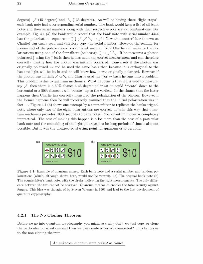
example, Fig. 4.1 (a) the bank would record that the bank note with serial number 4444
has the polarization sequence ↔ l l րւ րւ տց ↔ րւ. Now the counterfeiter (known as
Charlie) can easily read and therefore copy the serial number. However the reading (or
measuring) of the polarizations is a different manner. Now Charlie can measure the po-
larizations using one of the four filters (or bases): l ↔ րւ տց. If he measures a photon
polarized l using the l basis then he has made the correct measurement and can therefore
correctly identify how the photon was initially polarized. Conversely if the photon was
originally polarized ↔ and he used the same basis then because it is orthogonal to the
basis no light will be let in and he will know how it was originally polarized. However if
the photon was initiallyրւ orտց and Charlie used the l or ↔ basis he runs into a problem.
This problem is due to quantum mechanics. What happens is that if l is used to measure,
say րւ, then there is a 50% chance a 45 degree polarization could “rotate” down to the
horizontal or a 50% chance it will “rotate” up to the vertical. In the chance that the latter
happens then Charlie has correctly measured the polarization of the photon. However if
the former happens then he will incorrectly assumed that the initial polarization was in
fact ↔. Figure 4.1 (b) shows one attempt by a counterfeiter to replicate the banks original
note, where only two of the eight polarizations are correct. It is in this way that quan-
tum mechanics provides 100% security to bank notes! Now quantum money is completely
impractical. The cost of making this happen is a lot more than the cost of a particular
bank note and the embedding of the light polarizations for long periods of time is also not
possible. But it was the unexpected starting point for quantum cryptography.
ACM E QUANTU M MONEY
SERIAL # 4444
10$ACM E QUANTU M MONEY
SERIAL # 4444
10$(a) (b)
Figure 4.1: Example of quantum money. Each bank note had a serial number and random po-
larizations (which, although shown here, would not be viewed). (a) The original bank note (b)
The counterfeiter’s bank note, with the circles indicating the right measurements. The only differ-
ence between the two cannot be observed! Quantum mechanics enables the total security against
forgery. This idea was thought of by Steven Wiesner in 1969 and lead to the first development of
quantum cryptography.
4.2.1 The No Cloning Theorem
Before we go into quantum cryptography you might ask why don’t we just copy or clone
the particular polarizations and then we can create a perfect counterfeit? This brings us
to the non cloning theorem
An unknown quantum state cannot be cloned

§4.3 Discrete Quantum Cryptography 23
An important consequence of this theorem1 is it stops Charlie from simply copying the
specific polarizations of the bank note. This is because they are unknown states, i.e.
Charlie did not prepare them himself. So the no cloning theorem does not stop Charlie
from copying it all, but it forbids him from perfectly copying it. A short proof of the no
cloning theorem follows. We have U(|α〉|0〉) = |α〉|α〉 2 along with U(|β〉|0〉) = |β〉|β〉 with
|β〉 6= |α〉. Now if we take the inner product we have 〈α|β〉 = 〈α|〈α|β〉|β〉, which is equal
to 〈α|β〉2 = 〈α|β〉. This equation has either 1 or 0 as the solutions. So if it is 1 then α and
β are equal and are the same state. And if it is equal to 0, then α and β are orthogonal
and are therefore distinguishable. Therefore we can only copy states that are orthogonal
to each other but there does not exist a universal cloning machine that is able to copy
all nonorthogonal arbitrary states. This is an important property that is inherent in any
eavesdropping attack in quantum cryptography.
4.3 Discrete Quantum Cryptography
After discussing Wiesner’s idea with him, Charles Bennett, a scientist from Bell Labs
in New York, continuously thought of his idea over the next few years. This lead to
Bennett and another scientist, Gilles Brassard, to come up with quantum cryptography
[16]. This form of cryptography, know known as discrete quantum cryptography [17],
deals with the building and distribution of the key rather than the secure transmission of
a message. Therefore quantum cryptography is also known as quantum key distribution.
Once quantum cryptography is used to generate a secure key, the one time pad (see
Chapter 3) from classical cryptography, is used to encrypt the message. This only works
because the key is generated from a random key - which is a requirement of the one time
pad. This discrete quantum cryptographic protocol became known as the BB84 protocol,
after the authors (Bennett and Brassard) and the year it was first published (1984).
4.3.1 The BB84 Protocol
Alice and Bob have at their disposal four possible photon polarizations l ↔ րւ տց. They
then allocate a bit value of 1 to the l րւ polarizations and a bit value of 0 to the ↔ տցpolarizations. From these four polarizations there are two possible orthogonal bases: +(or
rectilinear) basis formed from the ↔ and l polarizations and the ×(or diagonal) basis
formed from the տց and րւ polarizations. The BB84 protocol goes as follows
1Even though one can clone a sheep, one cannot clone a single photon! - Andrew Steane2U here is known in quantum mechanics as the unitary operator. There is no need to go into detail
about this operator except to say that in our case its function is to evolve a ket in time.
24 Quantum Cryptography
1. Alice sends a random ensemble chosen from the four polarizations ↔, lրւտց.
2. Bob measures the ensemble Alice has sent by randomly switching between the
+ × bases.
3. Alice tells Bob (over a classically insecure channel) at which times he measured
the correct bases.
4. Alice and Bob discard the times when they did not use the same bases.
5. Alice and Bob then test the security of their key by using a randomly chosen
subset of their key. Results of their subset are compared and if errors are
detected, the transmission is insecure and they abort and start again.
6. Classical key distillation and privacy amplification techniques are used to gen-
erate a secure key.
7. The one time pad is used to encrypt a message.
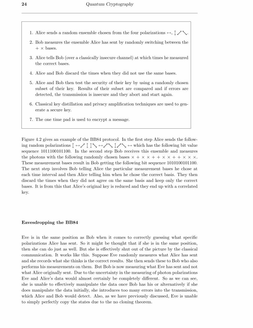
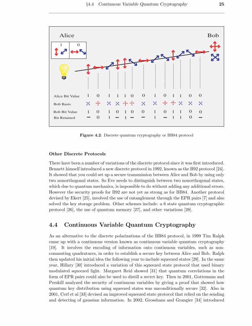
Figure 4.2 gives an example of the BB84 protocol. In the first step Alice sends the follow-
ing random polarizations l ↔րւ l lտց ↔րւտց lրւտց ↔ which has the following bit value
sequence 1011100101100. In the second step Bob receives this ensemble and measures
the photons with the following randomly chosen bases × + × × + + × × + + × × ×.
These measurement bases result in Bob getting the following bit sequence 1010100101100.
The next step involves Bob telling Alice the particular measurement bases he chose at
each time interval and then Alice telling him when he chose the correct basis. They then
discard the times when they did not agree on the same basis and keep only the correct
bases. It is from this that Alice’s original key is reduced and they end up with a correlated
key.
Eavesdropping the BB84
Eve is in the same position as Bob when it comes to correctly guessing what specific
polarizations Alice has sent. So it might be thought that if she is in the same position,
then she can do just as well. But she is effectively shut out of the picture by the classical
communication. It works like this. Suppose Eve randomly measures what Alice has sent
and she records what she thinks is the correct results. She then sends these to Bob who also
performs his measurements on them. But Bob is now measuring what Eve has sent and not
what Alice originally sent. Due to the uncertainty in the measuring of photon polarizations
Eve and Alice’s data would almost certainly be completely different. So as we can see,
she is unable to effectively manipulate the data once Bob has his or alternatively if she
does manipulate the data initially, she introduces too many errors into the transmission,
which Alice and Bob would detect. Also, as we have previously discussed, Eve is unable
to simply perfectly copy the states due to the no cloning theorem.
§4.4 Continuous Variable Quantum Cryptography 25
1 0
Alice Bob
Alice Bit Value 1 111111 000000
Bob Basis
Bob Bit Value
Bit Retained
1 11111
0
0 0 0
11111 0
0000
Figure 4.2: Discrete quantum cryptography or BB84 protocol
Other Discrete Protocols
There have been a number of variations of the discrete protocol since it was first introduced.
Bennett himself introduced a new discrete protocol in 1992, known as the B92 protocol [24].
It showed that you could set up a secure transmission between Alice and Bob by using only
two nonorthogonal states. So Eve needs to distinguish between two nonorthogonal states,
which due to quantum mechanics, is impossible to do without adding any additional errors.
However the security proofs for B92 are not yet as strong as for BB84. Another protocol
devised by Ekert [25], involved the use of entanglement through the EPR pairs [7] and also
solved the key storage problem. Other schemes include: a 6 state quantum cryptographic
protocol [26], the use of quantum memory [27], and other variations [28].
4.4 Continuous Variable Quantum Cryptography
As an alternative to the discrete polarizations of the BB84 protocol, in 1999 Tim Ralph
came up with a continuous version known as continuous variable quantum cryptography
[19]. It involves the encoding of information onto continuous variables, such as non-
commuting quadratures, in order to establish a secure key between Alice and Bob. Ralph
then updated his initial idea the following year to include squeezed states [29]. In the same
year, Hillary [30] introduced a variation of this squeezed state protocol that used binary
modulated squeezed light. Margaret Reid showed [31] that quantum correlations in the
form of EPR pairs could also be used to distill a secret key. Then in 2001, Gottesman and
Preskill analyzed the security of continuous variables by giving a proof that showed how
quantum key distribution using squeezed states was unconditionally secure [32]. Also in
2001, Cerf et al [33] devised an improved squeezed state protocol that relied on the sending
and detecting of gaussian information. In 2002, Grosshans and Grangier [34] introduced

26 Quantum Cryptography
a new continuous variable protocol that used coherent states instead of squeezed states.
They showed that coherent states afforded the same degree of security as compared to
protocols that used squeezed light and entanglement.
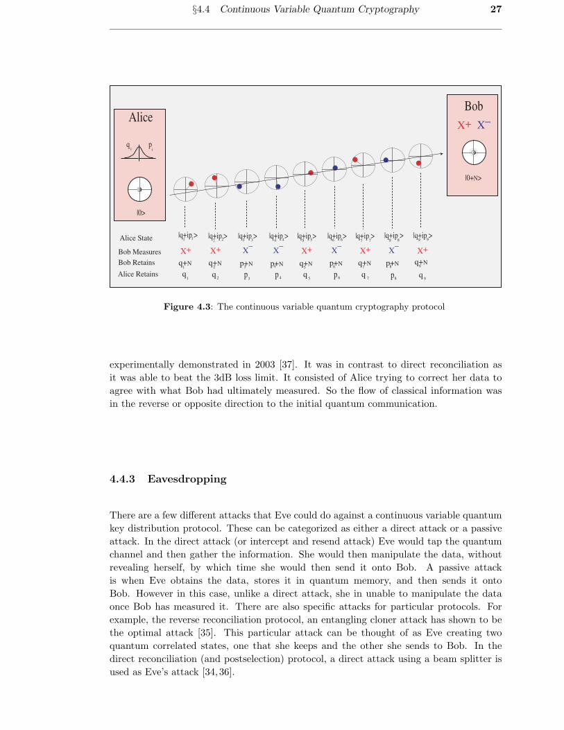
4.4.1 Steps of the Protocol
The protocol of the continuous regime is similar to that of the discrete regime and deals
with gaussian distributions and gaussian statistics in general. This is an important point,
as all analysis used in this thesis, use formulae and equations that are dependent on the
fact that we start off with and ultimately measure gaussian distributions. The continuous
variable version of our protocol is based on the one developed by Grosshans and Grang-
ier [34] and goes as follows:
1. Alice draws two real random numbers q and p from a gaussian distribution.
2. She displaces a vacuum state |0〉 by p and q to form a new random state
|q + ip〉.
3. Alice repeats steps (1) and (2) a number of times, sending the states to Bob.
4. Bob randomly switches between the measurement bases Q and P.
5. Bob tells Alice, over an insecure classical line, what basis he chose to measure
at each particular time interval.
6. Classical key distillation and privacy amplification techniques are used to gen-
erate a secure key.
7. Alice and Bob then test the security of their key by using a randomly chosen
subset of their key. Results of their subset are compared and if errors are
detected, the transmission is insecure and they abort and start again.
8. The one time pad is used to encrypt a message.
The allocation of bits for the continuous variable system is achieved during the key distilla-
tion section (see Section 4.5). Two particular continuous variable quantum cryptography
protocols are direct reconciliation and reverse reconciliation.
4.4.2 Direct and Reverse Reconciliation Protocols
The protocol above is an example of direct reconciliation as introduced by Grosshans
and Grangier [35]. This is where Bob has to correct his data to agree with what Alice
has sent. So the classical communication is in the same direction as the initial quantum
communication. Now direct reconciliation, and all previous protocols up until that point,
were thought to be secure for only line transmissions greater than 50% or 3dB line loss.
The first protocol that was shown to beat the 3dB loss limit was using postselection [36].
This is where Alice and Bob post select a subset of their data that they known is entirely
secure from Eve. Postselection is durable under high losses and is discussed in more
detail in Chapter 6. Reverse reconciliation was theoretically revealed in 2002 [35] and
§4.4 Continuous Variable Quantum Cryptography 27
Bob
X+ X_
Alice State
Bob Measures
Alice Retains
Bob Retains
X+ X_Alice
|0>
|q+ip >
q p
X+X+X+ X_
X_
X_
X+
q+N
q
|0+N>
p ppp qqqq
q+Nq+Nq+Nq+N p+N p+Np+Np+N
|q+ip >|q+ip >|q+ip >|q+ip >|q+ip >|q+ip >|q+ip >|q+ip >1
1
1
1
2 876543 9
2
22
3
33
4
44
5
55
6
66
7
77
8
88
9
99
i i
Figure 4.3: The continuous variable quantum cryptography protocol
experimentally demonstrated in 2003 [37]. It was in contrast to direct reconciliation as
it was able to beat the 3dB loss limit. It consisted of Alice trying to correct her data to
agree with what Bob had ultimately measured. So the flow of classical information was
in the reverse or opposite direction to the initial quantum communication.
4.4.3 Eavesdropping
There are a few different attacks that Eve could do against a continuous variable quantum
key distribution protocol. These can be categorized as either a direct attack or a passive
attack. In the direct attack (or intercept and resend attack) Eve would tap the quantum
channel and then gather the information. She would then manipulate the data, without
revealing herself, by which time she would then send it onto Bob. A passive attack
is when Eve obtains the data, stores it in quantum memory, and then sends it onto
Bob. However in this case, unlike a direct attack, she in unable to manipulate the data
once Bob has measured it. There are also specific attacks for particular protocols. For
example, the reverse reconciliation protocol, an entangling cloner attack has shown to be
the optimal attack [35]. This particular attack can be thought of as Eve creating two
quantum correlated states, one that she keeps and the other she sends to Bob. In the
direct reconciliation (and postselection) protocol, a direct attack using a beam splitter is
used as Eve’s attack [34,36].
28 Quantum Cryptography
4.5 Key Distillation and Privacy Amplification
I like my privacy.
- Shrek
This section will cover some concepts that are used once a raw key has been exchanged.
These are no longer quantum mechanical techniques but are purely classical in nature.
These include the correcting of errors between Alice and Bob (key distillation) and reducing
Eve’s knowledge of the final key (privacy amplification).
Key Distillation
The main point of key distillation is to produce a key between Alice and Bob which has
negligible errors. Eve also has the key but with many more errors. The two key distillation
techniques that will be used or are mentioned in this thesis, include reverse reconciliation
(see Chapter 5) and postselection (see Chapter 6). The allocation of bits in the BB84
protocol is agreed upon before Alice sends her ensemble. In the continuous variable version,
the allocation of bits occurs after Bob has recorded his results. One example of this is
the “sliced reconciliation” protocol [38]. This process can be thought of as the extraction
of a binary key from a gaussian distribution. The slice reconciliation protocol gives up
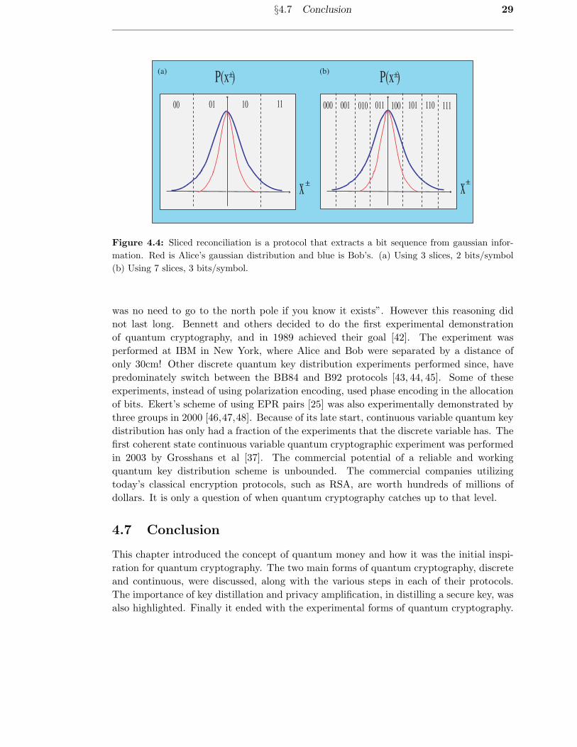
to 95% of the Shannon’s limit (see Chapter 5). Figure 4.4 gives an illustration of the
sliced reconciliation protocol. Alice has a gaussian distribution (red/thin line) from the
data that she has sent and Bob has the corresponding gaussian distribution (blue/thick
line). This is the same as Alice’s data, except that it has noise added on and so is a wider
distribution. Alice and Bob then divide their data into n slices3. Therefore there would
be n slices, with n+1 regions or bins, and n-1 bits/symbol. Examples with n=3 and n=7
are given in Fig. 4.4.
Privacy Amplification
Privacy amplification, as its name suggests, is a classical process where Alice and Bob
reduce Eve’s knowledge of the key to zero and therefore maintain their privacy. Privacy
amplification was first reported in 1988 by Bennett et al. [39,40]. This was then extended a
few years later and has also lead to interest from the classical cryptography community [41].
4.6 Experimental Quantum Cryptography
There was never any doubt that it would work, only that our
fingers would be too clumsy to build it.
- Charles Bennett
Charles Bennett was continually asked about whether the idea that he and Gilles Brassard
came up with, could be put into practice. For years he would always reply that “there
3These slices in practice would not be equal in length as they are in Fig. 4.4. Each region or bin, as itis known, would need to contain equal areas underneath the graph. This is so each bit of data is weightedequally.
§4.7 Conclusion 29
x
P(x )
x
P(x )(a) (b)
+_
_+ _+
_+
00 01 10 11 000 001 011010 100 101 110 111
Figure 4.4: Sliced reconciliation is a protocol that extracts a bit sequence from gaussian infor-
mation. Red is Alice’s gaussian distribution and blue is Bob’s. (a) Using 3 slices, 2 bits/symbol
(b) Using 7 slices, 3 bits/symbol.
was no need to go to the north pole if you know it exists”. However this reasoning did
not last long. Bennett and others decided to do the first experimental demonstration
of quantum cryptography, and in 1989 achieved their goal [42]. The experiment was
performed at IBM in New York, where Alice and Bob were separated by a distance of
only 30cm! Other discrete quantum key distribution experiments performed since, have
predominately switch between the BB84 and B92 protocols [43, 44, 45]. Some of these
experiments, instead of using polarization encoding, used phase encoding in the allocation
of bits. Ekert’s scheme of using EPR pairs [25] was also experimentally demonstrated by
three groups in 2000 [46,47,48]. Because of its late start, continuous variable quantum key
distribution has only had a fraction of the experiments that the discrete variable has. The
first coherent state continuous variable quantum cryptographic experiment was performed
in 2003 by Grosshans et al [37]. The commercial potential of a reliable and working
quantum key distribution scheme is unbounded. The commercial companies utilizing
today’s classical encryption protocols, such as RSA, are worth hundreds of millions of
dollars. It is only a question of when quantum cryptography catches up to that level.
4.7 Conclusion
This chapter introduced the concept of quantum money and how it was the initial inspi-
ration for quantum cryptography. The two main forms of quantum cryptography, discrete
and continuous, were discussed, along with the various steps in each of their protocols.
The importance of key distillation and privacy amplification, in distilling a secure key, was
also highlighted. Finally it ended with the experimental forms of quantum cryptography.

30 Quantum Cryptography
Chapter 5
Quantum Cryptography Without
Basis Switching
With quantum states, what we achieve
Defeats whatever you conceive.
So even Bob has to believe
That you can’t hear us, can you Eve?”
- John Preskill
This chapter investigates a new coherent state quantum key distribution protocol that
eliminates the need to randomly switch between measurement bases. This protocol pro-
vides significantly higher secret key rates with increased bandwidths than previous schemes
that only make single quadrature measurements. It also offers the further advantage of
simplicity compared to all previous protocols which, to date, have relied on switching.
The work presented here has been published in the journal article:
• Christian Weedbrook, Andrew Lance, Warwick Bowen, Thomas Symul, Tim Ralph
and Ping Koy Lam. Quantum Cryptography Without Switching, Physical Review
Letters 93, 170504 (2004).
5.1 Introduction
As we have seen from previous chapters, quantum cryptography is the science of sending
secret messages via a quantum channel. It uses properties of quantum mechanics [17, 18]
to establish a secure key, a process known as quantum key distribution [16]. This key
can then be used to send encrypted information. In a generic quantum key distribution
protocol, a sender (Alice) prepares quantum states which are sent to a receiver (Bob)
through a potentially noisy channel. Alice and Bob agree on a set of non-commuting bases
to measure the states with. Using various reconciliation [49,50] and privacy amplification
procedures [9], the results of measurements in these bases are used to construct a secret
key, known only to Alice and Bob. Switching randomly between a pair of non-commuting
measurement bases ensures security: in a direct attack, an eavesdropper (Eve) will only
choose the correct basis half the time; alternatively, if Eve uses quantum memory and
performs her measurements after Bob declares his basis, she is unable to manipulate what
Bob measures. It is commonly assumed that randomly switching between measurement
bases is crucial to the success of quantum key distribution protocols. In this chapter we
31
32 Quantum Cryptography Without Basis Switching
show that this is not the case, and in fact greater secret key rates can be achieved by
simultaneously measuring both bases.
The original quantum key distribution schemes in the discrete variable regime were
based on the transmission and measurement of random polarizations of single photon
states [17]. Other discrete variable quantum key distribution protocols have been pro-
posed [25] and experimentally demonstrated [46] using Bell states. However the band-
width of such schemes is experimentally limited by single photon generation and detection
techniques. Consequently in the last few years there has been considerable interest in
the field of continuous variable quantum cryptography [51], which provides an alternative
to the discrete approach and promises higher key rates. Continuous variable quantum
key distribution protocols have been proposed for squeezed and Einstein-Podolsky-Rosen
entangled states (see Chapter 4). However, these protocols require significant quantum
resources and are susceptible to decoherence due to losses. Quantum key distribution
protocols using coherent states were proposed to overcome these limitations. Originally
such schemes were only secure for line losses less than 50% or 3dB [29,34]. This apparent
limitation was overcome using the secret key distillation techniques of post-selection [36]
and reverse reconciliation [35].
S+
S-
Ν±B
X+B
X-
B
+
-
Laser
N±
η
Alice Bob
AM PM
Quantum channelX
±A
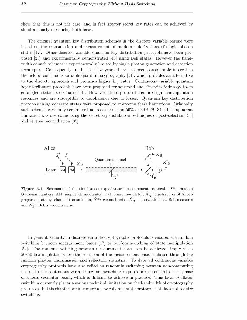
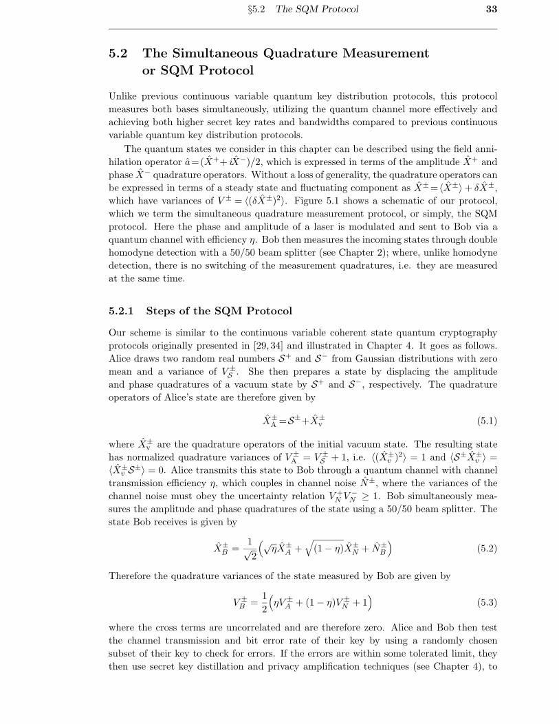
Figure 5.1: Schematic of the simultaneous quadrature measurement protocol. S±: random
Gaussian numbers, AM: amplitude modulator, PM: phase modulator, X±
A : quadratures of Alice’s
prepared state, η: channel transmission, N±: channel noise, X±
B : observables that Bob measures
and N±
B : Bob’s vacuum noise.
In general, security in discrete variable cryptography protocols is ensured via random
switching between measurement bases [17] or random switching of state manipulation
[52]. The random switching between measurement bases can be achieved simply via a
50/50 beam splitter, where the selection of the measurement basis is chosen through the
random photon transmission and reflection statistics. To date all continuous variable
cryptography protocols have also relied on randomly switching between non-commuting
bases. In the continuous variable regime, switching requires precise control of the phase
of a local oscillator beam, which is difficult to achieve in practice. This local oscillator
switching currently places a serious technical limitation on the bandwidth of cryptography
protocols. In this chapter, we introduce a new coherent state protocol that does not require
switching.
§5.2 The SQM Protocol 33
5.2 The Simultaneous Quadrature Measurement
or SQM Protocol
Unlike previous continuous variable quantum key distribution protocols, this protocol
measures both bases simultaneously, utilizing the quantum channel more effectively and
achieving both higher secret key rates and bandwidths compared to previous continuous
variable quantum key distribution protocols.
The quantum states we consider in this chapter can be described using the field anni-
hilation operator a=(X++ iX−)/2, which is expressed in terms of the amplitude X+ and
phase X− quadrature operators. Without a loss of generality, the quadrature operators can
be expressed in terms of a steady state and fluctuating component as X±=〈X±〉+ δX±,
which have variances of V ± = 〈(δX±)2〉. Figure 5.1 shows a schematic of our protocol,
which we term the simultaneous quadrature measurement protocol, or simply, the SQM
protocol. Here the phase and amplitude of a laser is modulated and sent to Bob via a
quantum channel with efficiency η. Bob then measures the incoming states through double
homodyne detection with a 50/50 beam splitter (see Chapter 2); where, unlike homodyne
detection, there is no switching of the measurement quadratures, i.e. they are measured
at the same time.
5.2.1 Steps of the SQM Protocol
Our scheme is similar to the continuous variable coherent state quantum cryptography
protocols originally presented in [29, 34] and illustrated in Chapter 4. It goes as follows.
Alice draws two random real numbers S+ and S− from Gaussian distributions with zero
mean and a variance of V ±S . She then prepares a state by displacing the amplitude
and phase quadratures of a vacuum state by S+ and S−, respectively. The quadrature
operators of Alice’s state are therefore given by
X±A =S±+X±
v (5.1)
where X±v are the quadrature operators of the initial vacuum state. The resulting state
has normalized quadrature variances of V ±A = V ±
S + 1, i.e. 〈(X±v )2〉 = 1 and 〈S±X±
v 〉 =
〈X±v S±〉 = 0. Alice transmits this state to Bob through a quantum channel with channel
transmission efficiency η, which couples in channel noise N±, where the variances of the
channel noise must obey the uncertainty relation V +N V −
N ≥ 1. Bob simultaneously mea-
sures the amplitude and phase quadratures of the state using a 50/50 beam splitter. The
state Bob receives is given by
X±B =
1√2
(√ηX±
A +√
(1 − η)X±N + N±
B
)
(5.2)
Therefore the quadrature variances of the state measured by Bob are given by
V ±B =
1
2
(
ηV ±A + (1 − η)V ±
N + 1)
(5.3)
where the cross terms are uncorrelated and are therefore zero. Alice and Bob then test
the channel transmission and bit error rate of their key by using a randomly chosen
subset of their key to check for errors. If the errors are within some tolerated limit, they
then use secret key distillation and privacy amplification techniques (see Chapter 4), to

34 Quantum Cryptography Without Basis Switching
distill a common secret key. This protocol is essentially the same as the one presented
in Section 4.4.1, except for the important fact that Bob now neglects the switching of
measurement bases, in favor of measuring both bases simultaneously. Another step that
has been changed is there is no need for Alice and Bob to classically differentiate which
quadratures were measured. It is possible to analyze our protocol using either the post-
0 0.2 0.4 0.6 0.8 11
2
3
4
5
Insecure Region
∆I≤0
∆I=0
12 34
Secure Region
∆I>0
Channel efficiency η
Ch
ann
el n
ois
e V
N
Figure 5.2: Contour plot of the information rate for the simultaneous quadrature measurement
protocol as a function of channel efficiency η and channel noise VN in units of (bits/symbol) for
VA = 100.
selection (see Chapter 6), or reverse reconciliation (see Chapter 4), secret key distillation
techniques. However, for simplicity, we limit our analysis to Grosshans and Grangier’s
reverse reconciliation protocol. In this protocol, both Alice and Eve, try to infer Bob’s
measurement results.
5.2.2 Conditional Variance
Alice’s inference can be characterized by a conditional variance which is used to calculate
the secret key rate. This conditional variance is defined as
V ±A|B = min
g±A
〈(X±B − g±AX±
A )2〉 (5.4)
and can be thought of as Alice giving her best estimate of what Bob has measured. This
is all inherent in the reverse reconciliation process. The gain g±A can be optimized to give
a minimum conditional variance. The optimization goes as follows
∂V ±A|B
g±A= − < X±
B X±A > − < X±
A X±B > +2g±A < X±2
A >= 0 (5.5)
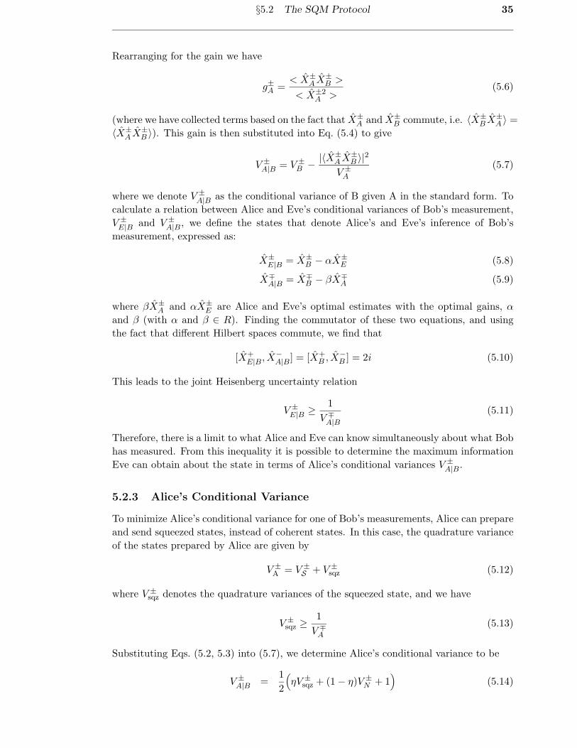
§5.2 The SQM Protocol 35
Rearranging for the gain we have
g±A =< X±
A X±B >
< X±2A >
(5.6)
(where we have collected terms based on the fact that X±A and X±
B commute, i.e. 〈X±B X±
A 〉 =
〈X±A X±
B 〉). This gain is then substituted into Eq. (5.4) to give
V ±A|B = V ±
B − |〈X±A X±
B 〉|2V ±
A
(5.7)
where we denote V ±A|B as the conditional variance of B given A in the standard form. To
calculate a relation between Alice and Eve’s conditional variances of Bob’s measurement,
V ±E|B and V ±
A|B, we define the states that denote Alice’s and Eve’s inference of Bob’s
measurement, expressed as:
X±E|B = X±
B − αX±E (5.8)
X∓A|B = X∓
B − βX∓A (5.9)
where βX±A and αX±
E are Alice and Eve’s optimal estimates with the optimal gains, α
and β (with α and β ∈ R). Finding the commutator of these two equations, and using
the fact that different Hilbert spaces commute, we find that
[X+E|B, X−
A|B] = [X+B , X−
B ] = 2i (5.10)
This leads to the joint Heisenberg uncertainty relation
V ±E|B ≥ 1
V ∓A|B
(5.11)
Therefore, there is a limit to what Alice and Eve can know simultaneously about what Bob
has measured. From this inequality it is possible to determine the maximum information
Eve can obtain about the state in terms of Alice’s conditional variances V ±A|B.
5.2.3 Alice’s Conditional Variance
To minimize Alice’s conditional variance for one of Bob’s measurements, Alice can prepare
and send squeezed states, instead of coherent states. In this case, the quadrature variance
of the states prepared by Alice are given by
V ±A = V ±
S + V ±sqz (5.12)
where V ±sqz denotes the quadrature variances of the squeezed state, and we have
V ±sqz ≥
1
V ∓A
(5.13)
Substituting Eqs. (5.2, 5.3) into (5.7), we determine Alice’s conditional variance to be
V ±A|B =
1
2
(
ηV ±sqz + (1 − η)V ±
N + 1)
(5.14)
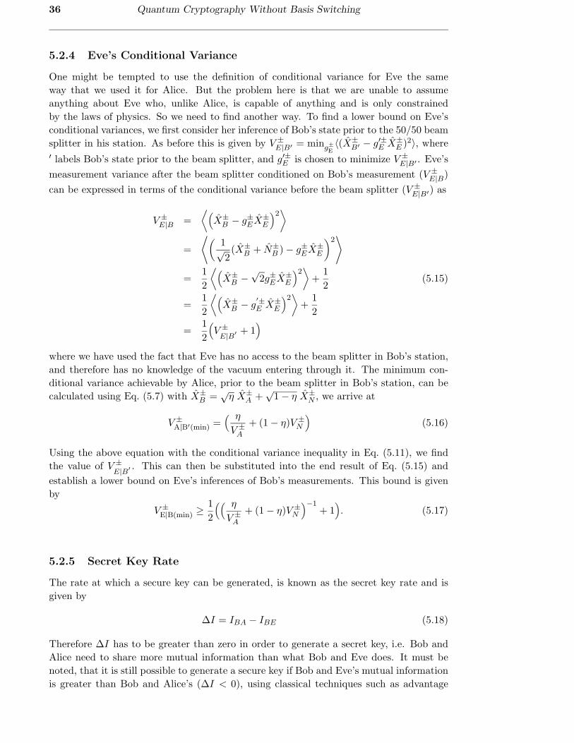
36 Quantum Cryptography Without Basis Switching
5.2.4 Eve’s Conditional Variance
One might be tempted to use the definition of conditional variance for Eve the same
way that we used it for Alice. But the problem here is that we are unable to assume
anything about Eve who, unlike Alice, is capable of anything and is only constrained
by the laws of physics. So we need to find another way. To find a lower bound on Eve’s
conditional variances, we first consider her inference of Bob’s state prior to the 50/50 beam
splitter in his station. As before this is given by V ±E|B′ = ming±
E
〈(X±B′ − g′±E X±
E )2〉, where′ labels Bob’s state prior to the beam splitter, and g′±E is chosen to minimize V ±
E|B′ . Eve’s
measurement variance after the beam splitter conditioned on Bob’s measurement (V ±E|B)
can be expressed in terms of the conditional variance before the beam splitter (V ±E|B′) as
V ±E|B =
⟨
(
X±B − g±EX±
E
)2⟩
=
⟨
(
1√2(X±
B + N±B ) − g±EX±
E
)2⟩
=1
2
⟨
(
X±B −
√2g±EX±
E
)2⟩
+1
2(5.15)
=1
2
⟨
(
X±B − g
′±E X±
E
)2⟩
+1
2
=1
2
(
V ±E|B′ + 1
)
where we have used the fact that Eve has no access to the beam splitter in Bob’s station,
and therefore has no knowledge of the vacuum entering through it. The minimum con-
ditional variance achievable by Alice, prior to the beam splitter in Bob’s station, can be
calculated using Eq. (5.7) with X±B =
√η X±
A +√
1 − η X±N , we arrive at
V ±A|B′(min) =
( η
V ±A
+ (1 − η)V ±N
)
(5.16)
Using the above equation with the conditional variance inequality in Eq. (5.11), we find
the value of V ±E|B′ . This can then be substituted into the end result of Eq. (5.15) and
establish a lower bound on Eve’s inferences of Bob’s measurements. This bound is given
by
V ±E|B(min) ≥
1
2
(( η
V ±A
+ (1 − η)V ±N
)−1+ 1
)
. (5.17)
5.2.5 Secret Key Rate
The rate at which a secure key can be generated, is known as the secret key rate and is
given by
∆I = IBA − IBE (5.18)
Therefore ∆I has to be greater than zero in order to generate a secret key, i.e. Bob and
Alice need to share more mutual information than what Bob and Eve does. It must be
noted, that it is still possible to generate a secure key if Bob and Eve’s mutual information
is greater than Bob and Alice’s (∆I < 0), using classical techniques such as advantage
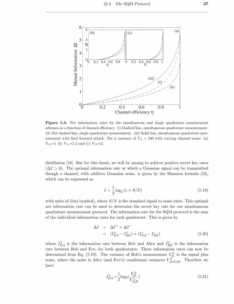
§5.2 The SQM Protocol 37
0 10
1
2
3
4
5
6
0.2 0.4 0.6 0.8
0 0.2 0.4 0.6 0.8 10 0.20
2
4
6
0.4 0.6 0.8
(a)(b) (c)
Channel efficiency η
Mu
tual
In
form
atio
n ∆I
η η
∆I(i)
(ii)
(iii)
Figure 5.3: Net information rates for the simultaneous and single quadrature measurement
schemes as a function of channel efficiency. (i) Dashed line, simultaneous quadrature measurement.
(ii) Dot dashed line, single quadrature measurement. (iii) Solid line, simultaneous quadrature mea-
surement with feed forward attack. For a variance of VA = 100 with varying channel noise: (a)
VN=1 (b) VN=1.2 and (c) VN=2.
distillation [16]. But for this thesis, we will be aiming to achieve positive secret key rates
(∆I > 0). The optimal information rate at which a Gaussian signal can be transmitted
though a channel, with additive Gaussian noise, is given by the Shannon formula [53],
which can be expressed as
I =1
2log2 (1 + S/N) (5.19)
with units of (bits/symbol), where S/N is the standard signal to noise ratio. This optimal
net information rate can be used to determine the secret key rate for our simultaneous
quadrature measurement protocol. The information rate for the SQM protocol is the sum
of the individual information rates for each quadrature. This is given by
∆I = ∆I+ + ∆I−
= (I+BA − I+
BE) + (I−BA − I−BE) (5.20)
where I±BA is the information rate between Bob and Alice and I±BE is the information
rate between Bob and Eve, for both quadratures. These information rates can now be
determined from Eq. (5.19). The variance of Bob’s measurement V ±B is the signal plus
noise, where the noise is Alice (and Eve’s) conditional variances V ±A(E)|B. Therefore we
have
I±BA =1
2log2(
V ±B
V ±A|B
) (5.21)
38 Quantum Cryptography Without Basis Switching
I±BE =1
2log2(
V ±B
V ±E|B
) (5.22)
Substituting these expressions into Eq. (5.20), the secret key rate for the simultaneous
quadrature measurement protocol can be expressed as
∆I =1
2log2
(V +E|BV −
E|BV +
A|BV −A|B
)
(5.23)
Substituting Eq. (5.14) with V ±sqz = 1 (Alice maximizes her information rate by using
coherent states), and Eq. (5.17) into Eq. (5.23), gives a lower bound on the secret key rate
∆I ≥ log2
(( ηVA
+ (1 − η)VN )−1 + 1
η + (1 − η)VN + 1
)
(5.24)
where we have assumed symmetry between the amplitude and phase quadratures. Fig-
ure 5.2 shows the secret key rate for the simultaneous quadrature measurement scheme
as a function of channel efficiency and channel noise. We see that, so long as the channel
noise VN is not excessive, a secret key can be successfully generated between Alice and
Bob, even in the limit of very small channel efficiency η. As the channel noise is reduced, or
efficiency increased, the rate at which a key can be established is enhanced. The different
shadings reveal the increase in information rate as the channel efficiency is increased. This
tends towards an information rate of just over 5.5 bits/symbol for perfect efficiency and a
coherent vacuum noise. Figure 5.3 compares the information rates of the SQM protocol
(dashed line) and single quadrature (dot dashed line) protocol, as a function of channel
efficiency. The two insets give the same comparison but for varying channel noises. In
each case, the information rate for the SQM protocol is always higher than that for single
quadrature measurement protocol. Also if Alice prepares her states with a large variance
(i.e. VA = 100) and with a high channel efficiency, the information rate for the SQM
protocol is two times that of the previous best switching scheme. Both schemes collapse
(i.e. become less secure) quickly when the channel noise is only slightly increased. This
is because we are using reverse reconciliation, which is unable to tolerate high loss. The
other solid line in this graph is a possible eavesdropping attack, which is discussed in the
next section. The individual secret key rates (i.e. IBA and IBE) for the simultaneous and
single quadrature measurement protocols can be calculated and are plotted in Fig. 5.5.
The shadings in each case, is the area between the individual information rates. Taking
the difference at each point gives the net information rate. Therefore a larger shaded area
indicates a larger information rate. Thus the SQM protocol clearly dominates the scheme
that uses switching in its protocol. It should be noted that in our protocol Eve must
attempt to determine Bob’s measurements in both the amplitude and phase quadratures
at the same time. This introduces an extra penalty to Eve, which is not included in the
lower bound for her conditional variance in Eq. (5.17). Therefore, in general, Eve will
do even worse than our analysis suggests. The dashed line on the graph is a possible
eavesdropping attack that is discussed next.
§5.3 Eavesdropping Attack 39
5.3 Eavesdropping Attack
Confound it all, Samwise Gamgee. Have you been eavesdropping?
- Gandalf, Fellowship of the Ring
To establish an upper bound on the secret key rate, we now consider the physical imple-
mentation of an eavesdropping attack for Eve for our protocol. In the case where Bob
measures a single quadrature, Grosshans and Grangier showed that an entangling cloner
attack is the optimum attack [35]. For the SQM protocol, we considered a number of
possible attacks for Eve, including various attacks where she injects entanglement into
the quantum channel, but found the most effective approach to be a simple feed forward
attack with no entanglement as shown in Fig. 5.4.
5.3.1 Feed Forward Protocol
The attack goes as follows: Eve taps off a fraction of the beam using a beam splitter with
transmission ǫ. She performs simultaneous quadrature measurements on this beam, with
measured quadratures of
X±E =
1√2
(√1 − ǫ X±
A +√
ǫ N±E1 + N±
E2
)
(5.25)
Therefore the quadrature variances of these states are
V ±E =
1
2
(
(1 − ǫ)V ±A + ǫ + 1
)
(5.26)
where we have normalized the two vacuums entering her beam splitters to one. She then
applies the measured photocurrents back onto the quantum channel using electronic feed
forward techniques with some gain g±E . Now because Eve has reduced the transmission
of the quantum channel, she will need to add additional Gaussian noise N± to remain
undetected. So after Bob has measured both quadratures simultaneously, he will have
X±B =
1√2
(
g±EX±E + N± +
√ǫX±
A +√
1 − ǫN±E1 + N±
B
)
(5.27)
where X±E is given in Eq (5.25). The variances of Bob’s measurements can then be ex-
pressed as
V ±B =
1
2
((√ǫ + g±E
√
(1 − ǫ)/2)2
V ±A + 1 (5.28)
+ V±N + g2±
E /2 +(√
1 − ǫ + g±E
√
ǫ/2)2)
The gain of Eve’s feed forward must be chosen carefully to ensure that the magnitude of
the signal detected by Bob remains invariant. So for an arbitrary channel transmission η,
Bob would be expecting a signal of√
η X±A . Now Eve knows that she is sending Bob a signal
of√
ǫ X±A +g±E
√
(1 − ǫ)/2 X±A . Therefore she wants
√η X±
A =√
ǫ X±A +g±E
√
(1 − ǫ)/2 X±A .
This leads to a gain of
g±E =
√2(√
η −√ǫ)√
1 − ǫ(5.29)
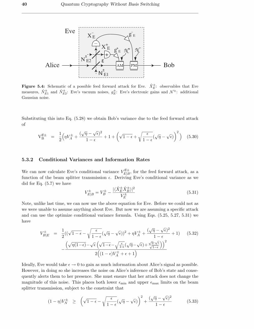
40 Quantum Cryptography Without Basis Switching
N+ N-
g+E
g-
E
AM PM
Ν±E1
N±E2 ε
Eve
Alice Bob
X+E
X-
E
+
-
Figure 5.4: Schematic of a possible feed forward attack for Eve. X±
E : observables that Eve
measures, N±
E1and N±
E2: Eve’s vacuum noises, g±E : Eve’s electronic gains and N±: additional
Gaussian noise.
Substituting this into Eq. (5.28) we obtain Bob’s variance due to the feed forward attack
of
Vff±B =
1
2
(
ηV ±A +
(√
η −√ǫ)2
1 − ǫ+ 1 +
(√1 − ǫ +
√
ǫ
1 − ǫ(√
η −√ǫ)
)2)
(5.30)
5.3.2 Conditional Variances and Information Rates
We can now calculate Eve’s conditional variance V ff±E|B, for the feed forward attack, as a
function of the beam splitter transmission ǫ. Deriving Eve’s conditional variance as we
did for Eq. (5.7) we have
V ±E|B = V ±
B − |〈X±E X±
B 〉|2V ±
E
(5.31)
Note, unlike last time, we can now use the above equation for Eve. Before we could not as
we were unable to assume anything about Eve. But now we are assuming a specific attack
and can use the optimize conditional variance formula. Using Eqs. (5.25, 5.27, 5.31) we
have
V ±B|E =
1
2((√
1 − ǫ −√
ǫ
1 − ǫ(√
η −√ǫ))2 + ηV ±
A +(√
η −√ǫ)2
1 − ǫ+ 1) (5.32)
−
(
√
η(1−ǫ)−√ǫ(√
1−ǫ−√
ǫ1−ǫ(
√η−√
ǫ)+√
η−√ǫ√1−ǫ
))2
2(
(1 − ǫ)V ±A + ǫ + 1
)
Ideally, Eve would take ǫ → 0 to gain as much information about Alice’s signal as possible.
However, in doing so she increases the noise on Alice’s inference of Bob’s state and conse-
quently alerts them to her presence. She must ensure that her attack does not change the
magnitude of this noise. This places both lower ǫmin and upper ǫmax limits on the beam
splitter transmission, subject to the constraint that
(1 − η)V ±N ≥
(√1 − ǫ −
√
ǫ
1 − ǫ(√
η −√ǫ)
)2
+(√
η −√ǫ)2
1 − ǫ(5.33)
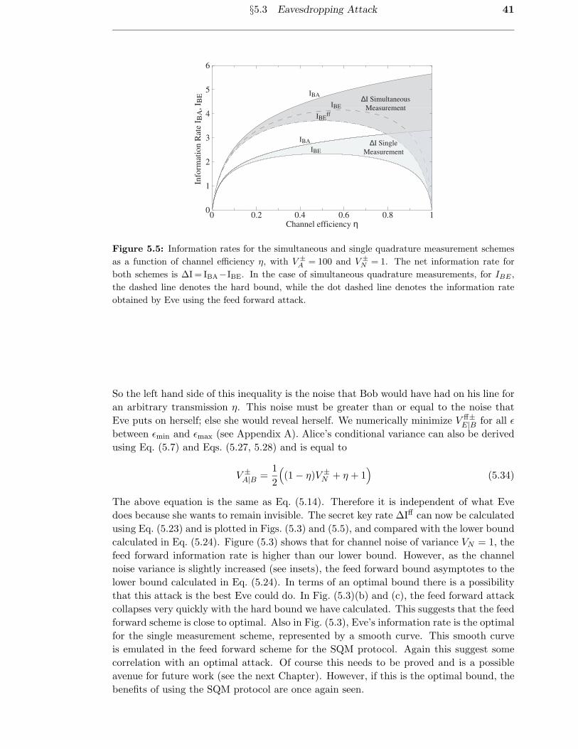
§5.3 Eavesdropping Attack 41
0 10
1
2
3
4
5
6
0.2 0.4 0.6 0.8Channel efficiency η
Info
rmat
ion R
ate
I BA
, I B
E
IBE
IBEff
IBA
IBA
∆I Simultaneous
Measurement
∆I Single
Measurement
IBE
Figure 5.5: Information rates for the simultaneous and single quadrature measurement schemes
as a function of channel efficiency η, with V ±
A = 100 and V ±
N = 1. The net information rate for
both schemes is ∆I = IBA−IBE. In the case of simultaneous quadrature measurements, for IBE ,
the dashed line denotes the hard bound, while the dot dashed line denotes the information rate
obtained by Eve using the feed forward attack.
So the left hand side of this inequality is the noise that Bob would have had on his line for
an arbitrary transmission η. This noise must be greater than or equal to the noise that
Eve puts on herself; else she would reveal herself. We numerically minimize V ff±E|B for all ǫ
between ǫmin and ǫmax (see Appendix A). Alice’s conditional variance can also be derived
using Eq. (5.7) and Eqs. (5.27, 5.28) and is equal to
V ±A|B =
1
2
(
(1 − η)V ±N + η + 1
)
(5.34)
The above equation is the same as Eq. (5.14). Therefore it is independent of what Eve
does because she wants to remain invisible. The secret key rate ∆Iff can now be calculated
using Eq. (5.23) and is plotted in Figs. (5.3) and (5.5), and compared with the lower bound
calculated in Eq. (5.24). Figure (5.3) shows that for channel noise of variance VN = 1, the
feed forward information rate is higher than our lower bound. However, as the channel
noise variance is slightly increased (see insets), the feed forward bound asymptotes to the
lower bound calculated in Eq. (5.24). In terms of an optimal bound there is a possibility
that this attack is the best Eve could do. In Fig. (5.3)(b) and (c), the feed forward attack
collapses very quickly with the hard bound we have calculated. This suggests that the feed
forward scheme is close to optimal. Also in Fig. (5.3), Eve’s information rate is the optimal
for the single measurement scheme, represented by a smooth curve. This smooth curve
is emulated in the feed forward scheme for the SQM protocol. Again this suggest some
correlation with an optimal attack. Of course this needs to be proved and is a possible
avenue for future work (see the next Chapter). However, if this is the optimal bound, the
benefits of using the SQM protocol are once again seen.
42 Quantum Cryptography Without Basis Switching
5.4 Conclusion
To summarize, we have proposed a new coherent state quantum key distribution protocol
based on simultaneous quadrature measurements. We have calculated a lower bound on
the secret key rate for this protocol, finding that in the limit of large signal variance and
high channel efficiency it approaches twice that of previous coherent state quantum key
distribution schemes. We have considered a possible eavesdropping attack in the form of
a simple feed forward scheme, which has provided us with an upper bound on the secret
key rate. An important advantage of our simultaneous quadrature measurement protocol
is the increase in total bandwidth. The absolute information rate, in bits/second, can be
expressed as I = W log2(1+S/N) [53], where W is the limiting bandwidth associated with
the state preparation or detection. Typically, in continuous variable quantum cryptogra-
phy schemes, W can be attributed to the switching time for the optical phase of the local
oscillator. The simultaneous quadrature measurement scheme does not require switching,
so that orders of magnitude increases in absolute secret key rates should be achievable.
In conclusion, we have shown that there is no need to randomly switch bases to achieve
secure quantum key distribution. By performing simultaneous quadrature measurements
in a coherent state quantum cryptography protocol, we are able to achieve a significantly
larger secret key rate than that obtained by the usual single quadrature measurements.
This new quantum key distribution protocol will allow simpler and higher bandwidth
quantum cryptographic experiments and technological applications.

Chapter 6
Conclusions and Future Work
The time-travelling is just too dangerous. Better that I devote myself to study
the other great mystery of the universe: women!
- Dr Emmett Brown, Back to the Future
6.1 Summary
In conclusion, we have introduced a new coherent state continuous variable quantum cryp-
tographic protocol, known as the simultaneous quadrature measurement protocol or the
SQM protocol. All previous quantum cryptography schemes, both discrete and continuous,
relied on a fundamental step in their protocols: basis switching. This step was thought
important in order to maintain an extra amount of security from any eavesdropper. We
have shown that this is not true. By eliminating the need to randomly switch bases,
we have shown that Alice and Bob can still build a secure secret key. Furthermore, by
measuring both quadratures simultaneously, we showed that the information rate is dou-
bled in the limit of high variance. Our protocol will also result in a simplification of any
experimental or commercial quantum cryptographic application, along with a significant
increase in bandwidth. The SQM protocol can also be applied to all previous continuous
variable quantum cryptographic protocols.
6.2 Future Work
A number of exciting future prospects have resulted from the research that was carried out
in this thesis. These include adapting the simultaneous quadrature measurement protocol
to other key distillation techniques such as postselection. As well as more fundamental
quantum information problems such as distinguishing between quantum states.
6.2.1 The SQM Protocol using Postselection
In previous chapters we discussed the concepts of reconciliation and privacy amplification
procedures. In this thesis we used reverse reconciliation which is just one possible way.
Another reconciliation and privacy amplification technique is postselection [36]. This is
when Alice and Bob post select a subset of their raw data - a subset that they know is
completely secure from Eve. Postselection results in much lower information rates than
reverse reconciliation, but it is able to tolerate significantly higher amounts of channel
43

44 Conclusions and Future Work
noise. We will briefly describe how postselection currently works, i.e. with Bob randomly
switching between his measurement bases.
Alice prepares an ensemble of quantum states from a possible choice of four coherent
states |αeiθ〉 | − αe−iθ〉 |iαeiθ〉 or | − iαe−iθ〉 which have been randomly displaced from
a vacuum state centered at the origin. Alice and Bob have previously agreed upon the
bit allocation where all the positively displaced states are a 0 and negative ones a 1, i.e.
|αeiθ〉 → 0, | − αe−iθ〉 → 1, |iαeiθ〉 → 0, | − iαe−iθ〉 → 1. She then sends this ensemble to
Bob who measures them using homodyne detection. He then randomly switches the basis
used to measure the quantum states. These measurements form two gaussian distributions
for both the amplitude and phase quadratures. These two distributions overlap at some
point creating a region of uncertainty. The quantum communication is now over and the
classical communication and thus reconciliation begins. The next step for Alice and Bob
is the securing of their raw key by putting a postselected threshold on their two gaussian
distributions. So they will keep any data over this threshold and allocate a bit value to
it, while all data within this region will be discarded. Another important point is that
because Bob and Eve’s information is uncorrelated, Eve has no way of knowing what this
threshold value is. Therefore the eavesdropper’s information is exponentially reduced to
zero.
A number of continuous variable quantum cryptographic papers have incorporated
postselection into their protocols [36, 54]. However all of these rely on basis switching.
Therefore future work could consist of adapting postsection to our simultaneous quadra-
ture measurement protocol.
6.2.2 Other Quantum Cryptographic Proposals
As we have seen from the last chapter, the question of an optimal bound is still unresolved.
An optimal bound is the maximum amount of information that Eve could obtain from
measuring both quadratures simultaneously. The determination of an optimal threshold
is directly linked to the concept of entropy and the accessible information of quantum
states [8]. Therefore our analysis in this thesis could also be transformed using entropic
relations - instead of the beam splitter equations - as a possible way of determining the
optimal bound. Further research could also consist of a comparison between the SQM pro-
tocol developed in this thesis and the information rates derived from the discrete variable
quantum cryptographic schemes.
6.2.3 The Accessible Information of Quantum States
There can’t be that much to say about two nonorthogonal states.
- Jeff Kimble
The accessible information of quantum states is not only applicable to quantum cryptog-
raphy but to quantum information in general. The only known case for the accessible
information (or mutual information)1 is for the simple two pure state case [56]. It is not
currently known for the general or mixed state cases. One of the main problems arises
from the difficulty in determining what the optimal measurement basis is for N states.
1see [8, 55] for an introduction to accessible information.
§6.3 Conclusion 45
6.3 Conclusion
Quantum information is one of the most exciting and rapidly developing fields in physics
today. It is based on the theory of quantum mechanics and has such diverse applications
as quantum computation, teleportation and quantum cryptography. This thesis has pre-
sented a new quantum cryptographic protocol that has eliminated a fundamental step that
all previous protocols were dependent on. And it is an example of the many possibilities
that lie ahead in quantum information theory.
46 Conclusions and Future Work

Appendix A
Matlab Code for Feed Forward
Optimization
The following code was written by Warwick Bowen. It is used in Chapter 5 to optimize
the feed forward scheme.
% Matlab code for Optimisation of Feed Forward
%% Use for Appendix of Thesis
clear all
%Variables
num=400; %resolution
etamin=0.0001; etamax=0.9999;
etavec=etamin:(etamax-etamin)/num:etamax;
eta=ones(size(etavec))’*etavec; %line efficiency
epsimin=0.0001; epsimax=0.9999;
epsivec=epsimin:(epsimax-epsimin)/num:epsimax;
epsi=(ones(size(epsivec))’*epsivec)’; %Eves beam splitter
\end{alltt}
Vn=1; %Channel noise
Vin=99; %Signal variance (Alice total variance = Vin+1)
%Working out what epsi’s are valid
F1=(1-eta)*Vn; F2=(sqrt(1-epsi) -
(sqrt(eta)-sqrt(epsi)).*sqrt(epsi./(1-epsi))).^2 +
(sqrt(eta)-sqrt(epsi)).^2./(1-epsi);
47

48 Matlab Code for Feed Forward Optimization
Error=0.000001;
check=(sign(F1-F2*(1-Error))+1)/2;
%Conditional variances
VBEa=0.5*(eta*(Vin+1)+(sqrt(1-epsi)-(sqrt(eta)-sqrt(epsi)).*sqrt(epsi./(1-epsi))).^2
+ (sqrt(eta)-sqrt(epsi)).^2./(1-epsi))+0.5;
VBEb=sqrt(eta.*(1-epsi))*(Vin+1) -
sqrt(epsi).*(sqrt(1-epsi)-(sqrt(eta)-sqrt(epsi)).*sqrt(epsi./(1-epsi)))+(sqrt(eta)-sqrt(epsi))./sqr
VBEc=2*((1-epsi)*Vin+2); VBE=VBEa-VBEb.^2./VBEc;
VBE=VBE+(1-check)*2^40;
VBA=0.5*(1+(1-eta)*Vn+eta);
exp=min(log2(VBE./VBA));

Bibliography
[1] S. Singh. The Code Book. Fourth Estate, London, 1999.
[2] D. Kahn. The Codebreakers. Sphere Books, London, 1974.
[3] C. Cohen-Tannoudji, Bernard Diu, and Franck Laloe. Quantum Mechanics. Wiley,
New York, 1977.
[4] D. Walls and G.J. Milburn. Quantum Optics. Springer, New York, 1994.
[5] H.A. Bachor and T.C. Ralph. A Guide to Experiments in Quantum Optics. Wiley-
VCH, Germany, 2002.
[6] M.O. Scully and M.S. Zubairy. Quantum Optics. Cambridge Unniversity Press, UK,
2002.
[7] A. Einstein, B. Podolsky, and N. Rosen. Can quantum-mechanical description of
physical reality be considered complete? Phys. Rev., 47:777, 1935.
[8] M.A. Nielsen and I.L. Chuang. Quantum information and quantum computation.
Canbridge University Press, Cambridge, UK, 2000.
[9] C.H. Bennett, G. Brassard, C. Crepeau, R. Jozsa, A. Peres, and W.K. Wooters.
Teleporting an unknown quantum state via dual classical and einstein-podolsky-rosen
channels. Phys. Rev. Lett., 70:1895, 1993.
[10] D. Deutsch. Quantum theory, the church-turing principle and the universal quantum
computer. Proc. Roy. Soc. Lond. A, 400:97, 1985.
[11] A. Steane. Quantum computing. Los Alamos ArXiv, http://arXiv.org/abs/quant-
ph/9708022, 1997.
[12] P.W. Shor. Phys. Rev. A, 52:R2493, 1995.
[13] C.H. Bennett and S.J. Wiesner. Communication via one-and two-particle operators
on einstein-podolsky-rosen states. Phys. Rev. Lett., 69:2881, 1992.
[14] L.K. Grover. Quantum mechanics helps in searching for a needle in a haystack. Phys.
Rev. Lett., 79:325, 1997.
[15] S.L. Braunstein and Arun K. Pati, editors. Quantum information with continuous
variables. Kluwer Academic Publishers, London, 2003.
[16] N. Gisin, G. Ribordy, W.Tittel, and H.Zbinden. Quantum cryptography. Rev. Mod.
Phys., 74:145, 2002.
[17] C.H. Bennet and G.Brassard. Quantum cryptography: Public key distribution and
coin tossing. Proceedings IEEE International Conference on Computers, Systems and
Signal Proceedings (Bangalore), pages 175–179, 1984.
49

50 Bibliography
[18] S.Wiesner. Conjugate coding. SIGACT News, 15:78, 1983.
[19] T.C. Ralph. Continuous-variable quantum cryptography. Phys. Rev. A, 61:010303,
1999.
[20] C. Weedbrook, A.M. Lance, W.P. Bowen, T. Symul, T.C. Ralph, and P.K. Lam.
Quantum cryptography without switching. Phys. Rev. Lett., 93:170504, 2004.
[21] P.K. Lam. Applications of quantum electro-optic control and squeezed light. PhD
Thesis, 1998.
[22] W.P. Bowen. Experiments towards a quantum information network with squeezed
light and entanglement. PhD Thesis, 2003.
[23] P.W. Shor. Polynomial-time algorithms for prime factorization and discrete loga-
rithms on a quantum computer. quant-ph/9508027, 1996.
[24] C.H. Bennett. Quantum cryptography using any two nonorthogonal states. Phys.
Rev. Lett., 68:3121, 1992.
[25] A. Ekert. Quantum cryptography based on bell’s theorem. Phys. Rev. Lett., 67:661,
1991.
[26] D. Bruss. Optimal eavesdropping in quantum cryptography with six states. Phys.
Rev. Lett., 81:3018, 1998.
[27] E. Biham, B. Huttner, and T. Mor. Quantum cryptographic network based on quan-
tum memories. Phys. Rev. A, 54:2651, 1996.
[28] P.D. Townsend. Quantum cryptography on multiuser optical fibre networks. Nature,
385:47, 1997.
[29] T.C. Ralph. Security of continuous-variable quantum cryptography. Phys. Rev. A,
62:062306, 2000.
[30] M. Hillery. Quantum cryptography with squeezed states. Phys. Rev. A, 61:022309,
2000.
[31] M.D. Reid. Quantum cryptography with a predetermined key, using continuous vari-
able einstein-podolsky-rosen correlations. Phys. Rev. A, 62:022309, 2000.
[32] D. Gottesman and J. Preskill. Secure quantum key distribution using squeezed states.
Phys. Rev. A, 63:022309, 2001.
[33] N.J. Cerf, M. Levy, and G. Van Assche. Quantum distribution of gaussian keys using
squeezed states. Phys. Rev. A, 63:052311, 2001.
[34] F. Grosshans and Ph. Grangier. Continuous variable quantum cryptography using
coherent states. Phys. Rev. Lett., 88:057902, 2002.
[35] F. Grosshans and P. Grangier. Reverse reconciliation protocols for quantum cryp-
tography with continous variables. Los Alamos ArXiv, http://arXiv.org/abs/quant-
ph/0204127, 2002.

Bibliography 51
[36] Ch. Silberhorn, T.C. Ralph, N. Lutkenhaus, and G. Leuchs. Continous variable
quantum cryptography: Beating the 3 db loss limit. Phys. Rev. Lett., 2002.
[37] F. Grosshans, G. Van Assche, J. Wenger, R. Brouri, N.J. Cerf, and Ph. Grangier.
Quantum key distribution using gaussian-modulated coherent states. Nature, 421:238,
2003.
[38] N.J. Cerf, M.Levy, and G. Van Assche. Phys. Rev. A, 63:052311, 2001.
[39] C.H. Bennett, G. Brassard, and J.M. Robert. Privacy amplification by public discus-
sion. SIAM J. Comp., 17:210, 1988.
[40] C.H. Bennett, G. Brassard, C. Crepeau, and U.M. Maurer. Generalized privacy
amplification. IEEE Trans. Information Th., 41:1915, 1995.
[41] U.M. Maurer and S. Wolf. Unconditionally secure key agreement and intrinsic infor-
mation. IEEE Transactions on Information Theory, 45:499, 1999.
[42] C.H. Bennett, F. Bessette, G. Brassard, L. Salvail, and J. Smolin. Experimental
quantum cryptography. Journal of Cryptology, 5:3, 1992.
[43] R.J. Hughes, D.M. Alde, P. Dyer, G.G. Luther, G.L. Morgan, and M. Schauer. Quan-
tum cryptography. Contemp. Phys., 36:149, 1995.
[44] G. Ribordy, J.D. Gautier, N. Gisin, O. Guinnard, and H. Zbinden. Fast and user-
friendly quantum key distribution. J. Modern Opt., 47:517, 2000.
[45] P. Townsend. Quantum cryptography on optical fibre networks. Opt. Fiber Tech.,
4:345, 1998.
[46] D. Naik, C. Peterson, A. White, A. Berglund, , and P. Kwiat. Entangled state quan-
tum cryptography: eavesdropping on the ekert protocol. Phys. Rev. Lett., 84:4733,
2000.
[47] T. Jennewein, C. Simon, G. Weihs, H. Weinfurter, and A. Zeilinger. Quantum cryp-
tography with entangled photons. Phys. Rev. Lett., 84:4729, 2000.
[48] W. Tittel, J. Brendel, H. Zbinden, and N. Gisin. Quantum cryptography using en-
tangled photons in energy-time bell states. Phys. Rev. Lett., 84:4737, 2000.
[49] U.M. Maurer. IEEE Trans. Inf. Theory, 39:733, 1993.
[50] G. Brassard and L. Salvail. Advances in cryptology-EUROCRYPT93, volume 765.
Springer-Verlag, 1994.
[51] T.C. Ralph. Quantum information theory with continuous variables, page 295.
Kluwer, Dordrecht, 2003.
[52] K. Bostrom and T. Felbinger. Deterministic secure direct communication using en-
tanglement. Phys. Rev. Lett., page 198902, 2002.
[53] C.E. Shannon. A mathematical theory of communication. Bell System Technical
Journal, 27:623, 1948.
52 Bibliography
[54] R. Namiki and T. Hirano. Security of quantum cryptography using balanced homo-
dyne detection. Phys. Rev. A, 67:022308, 2003.
[55] C.A. Fuchs. Phd thesis: Distinguishability and accessible information in quantum
theory. Los Alamos ArXiv, http://arXiv.org/abs/quant-ph/9601020, 1995.
[56] L.B. Levitin. Quantum communications and measurements, page 439. Plenum Press,
1995.
Index
Alice, Bob and Eve, 15
ball and stick picture, 9
BB84 protocol, 23
beam splitter, 11
classical cryptography, 15
coherent state, 9
commutator, 7
conditional variance, 34
cryptology, 15
detection, direct, 12
detection, standard homodyne , 12
key, 15
key distillation, 28
key distribution, 17
no cloning theorem, 22
one-time pad, 17
phase space representation, 8
plaintext, 15
postselection, 43
privacy amplification, 28
private key distribution, 17
public key distribution, 18
quadratures, 8
quantum cryptography, 21
quantum cryptography, continuous vari-
able, 25
quantum cryptography, discrete, 23
quantum cryptography, experimental, 28
quantum money, 21
reconciliation, direct, 26
reconciliation, reverse, 26
RSA code, 18
scytale, 16
secret key rate, 37
Shannon formula, 37
Shor’s algorithm, 19
SQM (Simultaneous Quadrature Measure-
ment) Protocol, 33
SQM, eavesdropping attack, 39
squeezing, 10
standard deviation, 8
steganography, 17
substitution, 16
transmission coefficient, 11
transposition, 16
uncertainty principle, 8
vacuum noise, 11
53