SciPost Phys. 4, 013 (2018)

Quantum dynamics in transverse-field Ising modelsfrom classical networks

Markus Schmitt1? and Markus Heyl2

1 Institute for Theoretical Physics, Georg-August-Universität Göttingen,Friedrich-Hund-Platz 1 - 37077 Göttingen, Germany

2 Max-Planck-Institute for the Physics of Complex Systems,Nöthnitzer Str. 38 - 01187 Dresden, Germany

? markus.schmitt@theorie.physik.uni-goettingen.de

Abstract

The efficient representation of quantum many-body states with classical resources isa key challenge in quantum many-body theory. In this work we analytically constructclassical networks for the description of the quantum dynamics in transverse-field Isingmodels that can be solved efficiently using Monte Carlo techniques. Our perturbativeconstruction encodes time-evolved quantum states of spin-1/2 systems in a network ofclassical spins with local couplings and can be directly generalized to other spin systemsand higher spins. Using this construction we compute the transient dynamics in one,two, and three dimensions including local observables, entanglement production, andLoschmidt amplitudes using Monte Carlo algorithms and demonstrate the accuracy ofthis approach by comparisons to exact results. We include a mapping to equivalent arti-ficial neural networks, which were recently introduced to provide a universal structurefor classical network wave functions.

Copyright M. Schmitt and M. Heyl.This work is licensed under the Creative CommonsAttribution 4.0 International License.Published by the SciPost Foundation.

Received 17-11-2017Accepted 16-02-2018Published 28-02-2018

Check forupdates

doi:10.21468/SciPostPhys.4.2.013

Contents

1 Introduction 2

2 Results 32.1 Classical network via cumulant expansion 32.2 Observables 42.3 Entanglement 62.4 Loschmidt amplitude 72.5 Construction of equivalent ANNs 9

3 Conclusions 10

A Perturbative classical networks 11

B Loschmidt amplitude as classical partition function 15

1

SciPost Phys. 4, 013 (2018)

C Exemplary derivation of ANN couplings from the cumulant expansion 18

References 20

1 Introduction

A key challenge in quantum many-body theory is the efficient representation of quantum many-body states using classical compute resources. The full information contained in such a many-body state in principle requires resources that grow exponentially with the number of degreesof freedom. Therefore, reliable schemes for the compression and efficient encoding of theessential information are vital for the numerical treatment of correlated systems with manydegrees of freedom. This is of particular relevance for dynamics far from equilibrium, wherelarge parts of the spectrum of the Hamiltonian play an important role.

For low-dimensional systems matrix product states [1,2] and more general tensor networkstates [3] constitute a powerful ansatz for the compressed representation of physically relevantmany-body wave functions. These allow for the efficient computation of ground states and realtime evolution. In high dimensions properties of quantum many-body systems in and out ofequilibrium can be obtained by dynamical mean field theory [4–7], which yields exact resultsin infinite dimensions. This leaves a gap at intermediate dimensions, where exciting physicsfar from equilibrium has recently been observed experimentally [8–13].

An alternative approach, which received increased attention lately, is the representation ofthe wave function based on networks of classical degrees of freedom. Given the basis vectors|~s⟩= |s1⟩⊗ |s2⟩⊗ . . .⊗|sN ⟩ of a many-body Hilbert space, where the sl label the local basis, thecoefficients of the wave function |ψ⟩ are expressed as

ψ(~s) = ⟨~s|ψ⟩= eH (~s), (1)

where H (~s) is an effective Hamilton function defining the classical network. Wave functionsof this form were used in combination with Monte Carlo algorithms for variational groundstate searches [14–16] and time evolution [17–23]. Recently, it was suggested that the wavefunction (1) can generally be encoded in an artificial neural network (ANN) trained to resem-ble the desired state [23]. This idea was seized in a series of subsequent works exploring thecapabilities of this and related representations [24–31]. Importantly, there are no principledrestrictions on dimensionality.

In this work we present a scheme to perturbatively derive analytical expressions for per-turbative classical networks (pCNs) as representation of time-evolved wave functions fortransverse-field Ising models (TFIMs) which can be extended directly also to other models. Theresulting networks consist of the same number of classical spins as the corresponding quan-tum system and exhibit only local couplings making the encoding particularly efficient. Wecompute the transient dynamics of the TFIM in one, two, and three dimensions (d = 1,2, 3)including local observables, correlation functions, entanglement production, and Loschmidtamplitudes. By comparing to exact solutions we demonstrate the accuracy of our results goingwell beyond standard perturbative approaches. This work provides a way to derive classicalnetwork structures within a constructive prescription, where other approaches rely on heuris-tics. As a specific application, we derive the structure and the time-dependent weights ofequivalent ANNs in the sense of Ref. [23].

2

SciPost Phys. 4, 013 (2018)

a© b©

Re(C

n)

0

Im(C

n)

t/tc

0

0 1 2 3 4 5 6

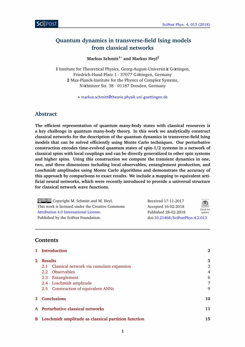
Figure 1: (a) Structure of the perturbative classical network for the TFIM in d = 2 and (b)dynamics of the couplings (color coded as in (a)). The black dots in the network structurerepresent a classical spin sl and its four neighbors in a translationally invariant square lattice.Each square with number n stands for a coupling of the connected classical spins with cou-pling constant Cn(t). The green and blue lines, respectively, correspond nearest-neighbor andnext-nearest-neighbor coupling of two spins, while the orange and red lines indicate couplingterms involving four spins each. The resulting time-dependent classical Hamiltonian functionH (~s, t) encodes quantum dynamics via Eq. (1).

2 Results

In the following we compute dynamics of TFIMs of N spins with Hamiltonian

H = −J4

∑

⟨i, j⟩

σziσ

zj −

h2

N∑

i=1

σxi , (2)

where σx/zi denote Pauli operators acting on site i and the first sum runs over neighboring

lattice sites i and j. As the computational basis we choose the spin basis states |~s⟩= |s1 . . . sN ⟩with si =↑,↓. The dynamics of Ising models is accessible experimentally with quantum simu-lators, which was demonstrated recently in various setups [32–34]. In d = 1 the dynamics ofthe TFIM can be computed analytically by means of a Jordan-Wigner transform [35–44].

In this work we are interested in the dynamics that comprise a dynamical quantum phasetransition (DQPT) [45, 46]. The signature of a DQPT is a non-analyticity in the many-bodydynamics analogous to equilibrium phase transitions where thermodynamic quantities behavenon-analytically as function of a control parameter. DQPTs were recently observed in experi-ment [11,34] and there is a series of results on TFIMs in this context [47–57].

Typically, DQPTs occur when the model is quenched across an underlying equilibrium quan-tum phase transition. A particularly insightful limit with this respect is a quench from h0 =∞to h/J 1, where, e.g., universal behavior was proven in d = 1 [51]. When quenching fromh0 =∞ to h = 0 the TFIM in d = 1,2 exhibits DQPTs at odd multiples of tc = π/J , whichwe choose as the unit of time throughout the paper. The ground state at h0 =∞ is a partic-ularly simple initial state, since ⟨~s|ψ0⟩ = 2−N/2. One could, however, go away from that limitperturbatively, e.g., by constructing a Schrieffer-Wolff transformation for an initial state withweak spin couplings.

Quench dynamics of the two-dimensional TFIM have already been studied in Refs. [20,21],but there quenches within the same phase have been considered in contrast to the extremequench across the phase boundary, which we will address in the following.

2.1 Classical network via cumulant expansion

Consider a Hamiltonian of the form H = H0 +λV , where H0 is diagonal in thespin basis, H0|~s⟩= E~s|~s⟩, V an off-diagonal operator, and λ 1. In the interaction

3

SciPost Phys. 4, 013 (2018)

picture the time evolution operator can be expressed as e−iHt = e−iH0 tWλ(t), whereWλ(t) = Tt exp

−iλ∫ t

0 d t ′V (t ′)

. In this setting time-evolved coefficients of the wave func-tion (1) can be obtained perturbatively by a cumulant expansion [58]. Denoting the initialstate with |ψ0⟩=

∑

~sψ0(~s)|~s⟩ the cumulant expansion to lowest order yields the time-evolvedstate |ψ(t)⟩=

∑

~sψ(~s, t)|~s⟩ with

ψ(~s, t)ψ0(~s)

= e−iE~s t exp

−iλ

∫ t

0

d t ′⟨~s|V (t ′)|ψ0⟩⟨~s|ψ0⟩

+O (λ2)

. (3)

By identifying H (~s, t) = −iE~s t − iλ∫ t

0 d t ′ ⟨~s|V (t′)|ψ0⟩

⟨~s|ψ0⟩the expression above takes the desired

form given in Eq. (1). Importantly, also the effective Hamilton function becomes local, when-ever H0 and V are local. It will be demonstrated below that the construction via cumulantexpansion yields much more accurate results than conventional perturbation theory. The ap-proximation can be systematically improved by taking into account higher order terms. Towhich extent it is possible to also capture long-time dynamics using such a construction, re-mains an open question and, since beyond the scope of the present work, will be left for futureresearch.

For our purposes, we identify H0 = −J4

∑

⟨i, j⟩σziσ

zj and λV = − h

2

∑

i σxi . Note that, e.g.,

a strongly anisotropic XXZ model could be treated analogously. The time-dependent V (t) isobtained by solving the Heisenberg equation of motion. The general form of the Hamiltonfunction from the first-order cumulant expansion obtained under these assumptions is

H (1)(~s, t) =z∑

n=0

Cn(t)N∑

l=1

∑

(a1,...,an)∈V ln

snl

n∏

r=1

sar, (4)

where V ln denotes the set of possible combinations of n neighboring sites of lattice site l, z is the

coordination number of the lattice, and Cn(t) are time-dependent complex couplings. ClassicalHamilton functions H (1)(~s, t) for cubic lattices in d = 1,2, 3 including explicit expressions forthe couplings Cn(t) are given in Appendix A. Fig. 1 displays the structure of the pCN in 2D andthe time evolution of the couplings Cn(t). For d = 2, 3 H (1)(~s, t) already contains couplingswith products of four or six spin variables, respectively. Thereby, the derived structure ofthe pCN markedly differs from heuristically motivated Jastrow-type wave functions, whichconstitute a common variational ansatz [17,20]. From our perturbative construction we findthat it is already at lowest order important to take into account plaquette interactions of morethan two spins in order to obtain accurate results.

The data we present in the following were obtained with h/J = 0.05. Results for largerh/J are presented in Appendix A. There we find that comparable accuracy is obtained fortimes ht 1. As we will show in the following the accuracy can be enhanced by includinghigher order contributions from the cumulant expansion. However, the resulting couplingparameters Cn(t) comprise secular terms, which grow with increasing time. We anticipatethat these secular terms restrict the time-window in which the couplings obtained from thecumulant expansions yield precise results to t < h−1. Nevertheless, we expect that an effectiveresummation of secular contributions can be achieved by combining the perturbatively derivednetwork structures with a time-dependent variational principle [17,59–61].

2.2 Observables

Plugging Eq. (1) into the time-dependent expectation value of an observable O with matrixelements ⟨~s|O|~s′⟩= O~sδ~s,~s′ results in

⟨ψ0|eiHtOe−iHt |ψ0⟩=∑

~s

eH (~s,t)O~s . (5)

4

SciPost Phys. 4, 013 (2018)

a© c©

b© d©

〈σx i〉

N = ∞ (exact)N = 50 (pCN-1)

N = 50 (pCN-2)N = 50 (tdPT)

0.0

0.5

1.0

N = 4× 4 (exact) N = 4× 4 (pCN)N = 8× 8× 8 (pCN)

〈σz iσz i+

1〉 t

×Jd

2h

t/tc

0.0

0.5

1.0

0 1 2 3 4 5 6

t/tc

0 1 2 3 4 5 6

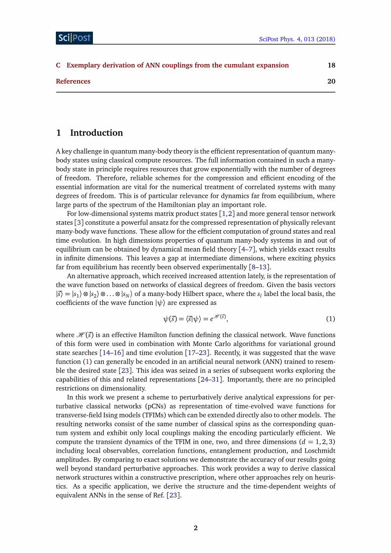
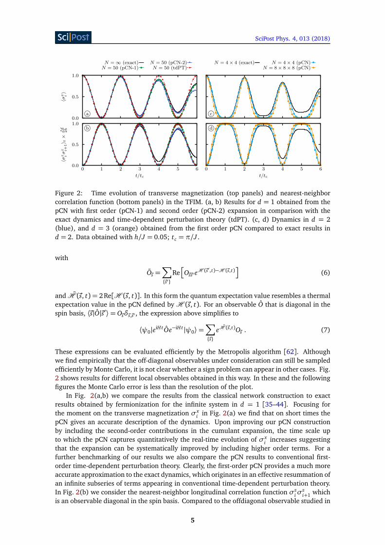
Figure 2: Time evolution of transverse magnetization (top panels) and nearest-neighborcorrelation function (bottom panels) in the TFIM. (a, b) Results for d = 1 obtained from thepCN with first order (pCN-1) and second order (pCN-2) expansion in comparison with theexact dynamics and time-dependent perturbation theory (tdPT). (c, d) Dynamics in d = 2(blue), and d = 3 (orange) obtained from the first order pCN compared to exact results ind = 2. Data obtained with h/J = 0.05; tc = π/J .

with

O~s =∑

~s′

Re

O~s~s′eH (~s′,t)−H (~s,t)

(6)

and H (~s, t) = 2Re[H (~s, t)]. In this form the quantum expectation value resembles a thermalexpectation value in the pCN defined by H (~s, t). For an observable O that is diagonal in thespin basis, ⟨~s|O|~s′⟩= O~sδ~s,~s′ , the expression above simplifies to

⟨ψ0|eiHtOe−iHt |ψ0⟩=∑

~s

eH (~s,t)O~s . (7)

These expressions can be evaluated efficiently by the Metropolis algorithm [62]. Althoughwe find empirically that the off-diagonal observables under consideration can still be sampledefficiently by Monte Carlo, it is not clear whether a sign problem can appear in other cases. Fig.2 shows results for different local observables obtained in this way. In these and the followingfigures the Monte Carlo error is less than the resolution of the plot.

In Fig. 2(a,b) we compare the results from the classical network construction to exactresults obtained by fermionization for the infinite system in d = 1 [35–44]. Focusing forthe moment on the transverse magnetization σx

i in Fig. 2(a) we find that on short times thepCN gives an accurate description of the dynamics. Upon improving our pCN constructionby including the second-order contributions in the cumulant expansion, the time scale upto which the pCN captures quantitatively the real-time evolution of σx

i increases suggestingthat the expansion can be systematically improved by including higher order terms. For afurther benchmarking of our results we also compare the pCN results to conventional first-order time-dependent perturbation theory. Clearly, the first-order pCN provides a much moreaccurate approximation to the exact dynamics, which originates in an effective resummation ofan infinite subseries of terms appearing in conventional time-dependent perturbation theory.In Fig. 2(b) we consider the nearest-neighbor longitudinal correlation function σz

iσzi+1 which

is an observable diagonal in the spin basis. Compared to the offdiagonal observable studied in

5

SciPost Phys. 4, 013 (2018)

a©a© b©Sn(t)/

log2

t/tc

N = ∞ (exact) N = 50 (pCN)N = 50 (tdPT)

0

1

2

0 1 2 3 4 5 6t/tc

N = 4× 4 (exact)N = 8× 8× 8

N = 4× 4

0 1 2 3 4 5 6t/tc

n = 8 n = 3× 2n = 3× 3

0

1

2

3

4

5

6

0 1 2 3 4 5 6

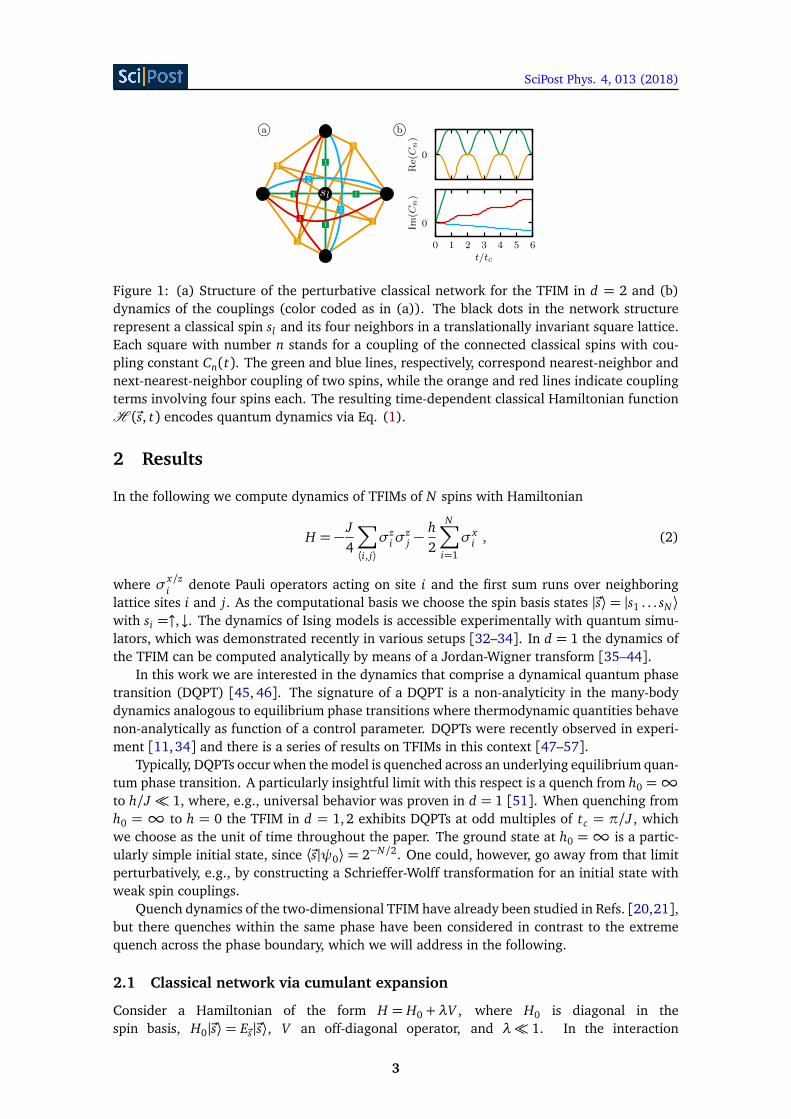
Figure 3: (a) Time evolution of the entanglement entropy for subsystems of n = 2 spinsobtained from the classical network by MC in comparison with exact results; h/J = 0.05.(b) Time evolution of the entanglement entropy for different subsystem shapes with n spinsobtained from full wave functions |ψ(t)⟩ determined from the pCN in comparison with exactresults (dashed lines). In d = 1 the system size is N = 20, in d = 2 it is N = 6×3; h/J = 0.05.

Fig. 2a we find much stronger deviations from the exact result which also cannot be improvedupon including higher orders in the cumulant expansion. However, for correlation functionsat longer distances the corrections to the first-order cumulant expansion become important;see Appendix A. The observation that the diagonal observables don’t improve with the orderof the pCN expansion we attribute to secular terms from resonant processes which are notappropriately captured by perturbative approaches such as the pCN. One possible strategy toincorporate such resonant processes is to impose a time-dependent variational principle [17,59–61] on our networks in order to obtain suitably optimized coupling coefficients. Havingdemonstrated under which circumstances the pCN can be improved by including higher ordercontributions, for the remainder of the article we focus on the capabilities of the first-orderpCN leaving further optimization strategies of the network open for the future.

In Fig. 2(c,d) we show our results for the same observables but now in d = 2 and d = 3.Compared to d = 1 we find much broader maxima and minima, respectively, close to thetimes where DQPTs occur at odd multiples of tc = π/J . In the limit h/J → 0 the shape isgiven by the power law |t − tc|z with z = 2d. This behavior was already observed for oneand two dimensional systems in Ref. [51]. For the d = 2 case we have included also exactdiagonalization data for a 4×4 lattice. Overall, we observe a similar accuracy in the dynamicsof these observables as compared to the d = 1 results.

2.3 Entanglement

Having discussed the capabilities of the pCN to encode the necessary information for the dy-namics of local observables and correlations, we would like to show now that it can also re-produce entanglement dynamics and thus the propagation of quantum information.

By sampling all correlation functions it is in principle possible to construct the re-duced density matrix of a subsystem A, ρA(t) = trB

|ψ(t)⟩⟨ψ(t)|

, where trB denotesthe trace over the complement of A, and the entanglement entropy of subsystem A givenby S(t) = −tr

ρA(t) lnρA(t)

. For subsystems with two spins at sites i and j we haveρA =

14

∑

α,α′∈0,x ,y,z⟨σαi σ

α′

j ⟩ σα ⊗σα

′, where σ0

i denotes the identity. This approach is in prin-

ciple applicable to arbitrary subsystem sizes; however, it quickly becomes unfeasible, becausethe number of correlation functions that has to be sampled grows exponentially with subsys-tem size. In order to obtain insights into the entanglement properties of larger subsystemsit might be possible to use the algorithm introduced in Ref. [63] for quantum Monte Carlo,which, however, is beyond the scope of this work. For small system sizes entanglement entropy

6

SciPost Phys. 4, 013 (2018)

for any block size can be extracted directly from the full wave function as described below.Figure 3(a) shows the entanglement entropy S2(t) of two neighboring spins. We find very

good agreement of the Monte Carlo data based on the first-order cumulant expansion with theexact results. In particular, for the entanglement entropy the classical network captures boththe decay of the maxima close to the critical times (2n+ 1)tc and the increase of the minima.As for the observables the shape in the vicinity of the maxima depends on d and is for h/J → 0given by the same power laws. Note, that the pCN correctly captures the maximal possibleentanglement Smax

2 = 2 ln2. By contrast, the result from tdPT completely misses the decay ofthe oscillations.

In order to assess the capability of the pCN to capture the entanglement dynamics of largersubsystems we compute the whole wave function |ψ(t)⟩ =

∑

~sψ(~s)|~s⟩ with the coefficientsψ(~s) as given in Eq. (3) for feasible system sizes. The entanglement entropy of arbitrarybipartitions is then obtained by a Schmidt decomposition. Fig. 3(b) shows entanglemententropies obtained in this way for subsystems of different sizes n in d = 1, 2. The results implythat at these short times only spins at the surface of the subsystem become entangled withthe rest of the system. The maxima for a subsystem of n = 8 spins in a ring of N = 20 spinsin d = 1 lie close to 2 ln 2, the theoretical maximum for the entanglement entropy of the twospins, which sit at the surface. This interpretation is supported by the results for a torus ofN = 6×3 spins with subsystems of size n= 3×2 and n= 3×3. In that case the entanglemententropy reaches maxima of 6 ln2, corresponding to 6 spins at the boundary. In both cases theresults agree well with the exact results for times t < 4tc . This again reflects the fact thatthe pCN from first-order cumulant expansion yields a good approximation of the dynamics ofneighboring spins.

2.4 Loschmidt amplitude

Next, we aim to show that not only local but also global properties are well-captured by theclassical networks. For that purpose we study the Loschmidt amplitude ⟨ψ0|ψ(t)⟩, whichconstitutes the central quantity for the anticipated DQPTs and which has been measured re-cently experimentally in different contexts [34, 64]. For a quench from h0 =∞ to h = 0 theLoschmidt amplitude

Z(t) =1

2N

∑

~s∈±1Nei J

4 t∑

⟨i, j⟩ sis j (8)

resembles the partition sum of a classical network with imaginary temperature β = −it [51].This expression is not suited for MC sampling because all weights lie on the unit circle inthe complex plane rendering importance sampling impractical and indicating a severe signproblem. These issues can be diminished by constructing an equivalent network with realweights. After integrating out every second spin on the sublattice Λ, equivalent to one deci-mation step [65], the partition sum takes the form

Z(t) =1

2N

∑

~s∈±1N/2

∏

i∈Λ2 cos

J4

t∑

⟨i, j⟩

s j

. (9)

Choosing a suited ansatz the partition sum can be rewritten as Z(t) =∑

~s eH (~s,t) with realBoltzmann weights given by an effective Hamilton function H (~s, t) that defines the classicalnetwork [51,65,66]. Generally, the effective Hamilton function takes the form

H (~s, t) =z/2∑

n=0

Cn(t)∑

l∈Λ

∑

(a1,...,a2n)∈V l2n

2n∏

r=1

sar. (10)

7

SciPost Phys. 4, 013 (2018)

a©

d = 1

b©

d = 3

b©b©

λN(t)

exactMC N = 100

0

ln 22

N = 4× 4× 4N = 4× 4× 6

Re(C

i)

t/tc

i = 1 i = 2

0

0 1 2t/tc

i = 3 i = 4

0 13

12

1 32

53

2

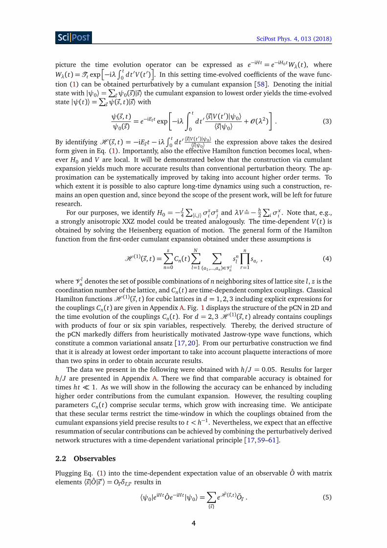
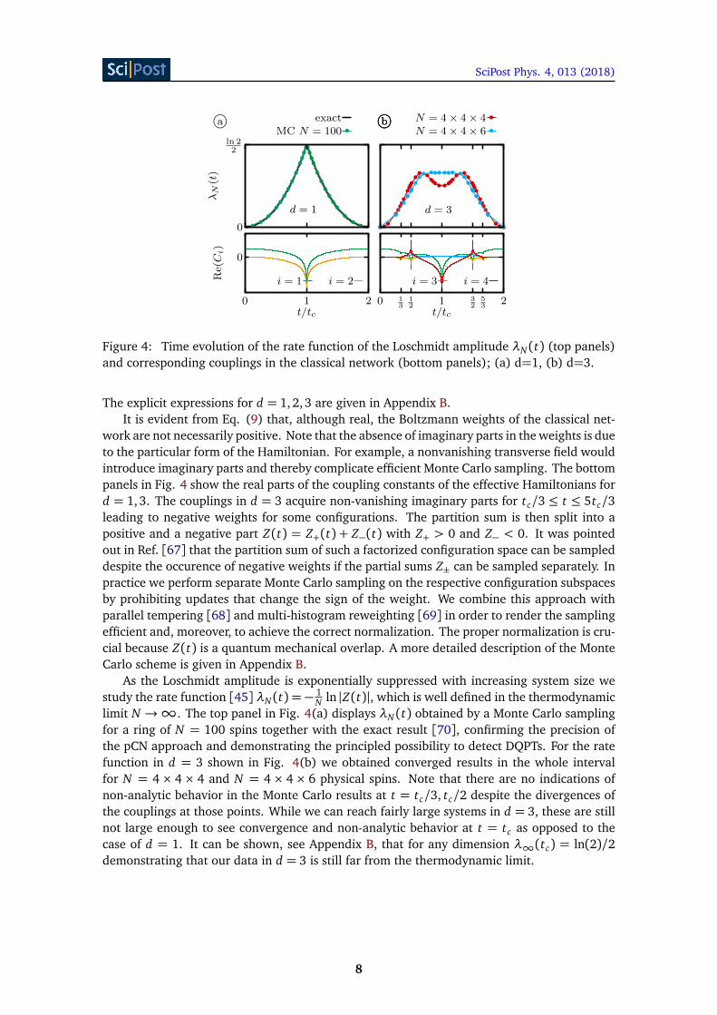
Figure 4: Time evolution of the rate function of the Loschmidt amplitude λN (t) (top panels)and corresponding couplings in the classical network (bottom panels); (a) d=1, (b) d=3.

The explicit expressions for d = 1, 2,3 are given in Appendix B.It is evident from Eq. (9) that, although real, the Boltzmann weights of the classical net-

work are not necessarily positive. Note that the absence of imaginary parts in the weights is dueto the particular form of the Hamiltonian. For example, a nonvanishing transverse field wouldintroduce imaginary parts and thereby complicate efficient Monte Carlo sampling. The bottompanels in Fig. 4 show the real parts of the coupling constants of the effective Hamiltonians ford = 1, 3. The couplings in d = 3 acquire non-vanishing imaginary parts for tc/3 ≤ t ≤ 5tc/3leading to negative weights for some configurations. The partition sum is then split into apositive and a negative part Z(t) = Z+(t) + Z−(t) with Z+ > 0 and Z− < 0. It was pointedout in Ref. [67] that the partition sum of such a factorized configuration space can be sampleddespite the occurence of negative weights if the partial sums Z± can be sampled separately. Inpractice we perform separate Monte Carlo sampling on the respective configuration subspacesby prohibiting updates that change the sign of the weight. We combine this approach withparallel tempering [68] and multi-histogram reweighting [69] in order to render the samplingefficient and, moreover, to achieve the correct normalization. The proper normalization is cru-cial because Z(t) is a quantum mechanical overlap. A more detailed description of the MonteCarlo scheme is given in Appendix B.

As the Loschmidt amplitude is exponentially suppressed with increasing system size westudy the rate function [45] λN (t) = −

1N ln |Z(t)|, which is well defined in the thermodynamic

limit N →∞. The top panel in Fig. 4(a) displays λN (t) obtained by a Monte Carlo samplingfor a ring of N = 100 spins together with the exact result [70], confirming the precision ofthe pCN approach and demonstrating the principled possibility to detect DQPTs. For the ratefunction in d = 3 shown in Fig. 4(b) we obtained converged results in the whole intervalfor N = 4 × 4 × 4 and N = 4 × 4 × 6 physical spins. Note that there are no indications ofnon-analytic behavior in the Monte Carlo results at t = tc/3, tc/2 despite the divergences ofthe couplings at those points. While we can reach fairly large systems in d = 3, these are stillnot large enough to see convergence and non-analytic behavior at t = tc as opposed to thecase of d = 1. It can be shown, see Appendix B, that for any dimension λ∞(tc) = ln(2)/2demonstrating that our data in d = 3 is still far from the thermodynamic limit.

8

SciPost Phys. 4, 013 (2018)

u(5)i,j u

(4)i,j

u(3)i,ju

(2)i,j

u(1)i,j

si,j

si,j+1

si,j−1

si+1,jsi−1,j

c© d©u(1)i

si si+1si−1

a© b©

Re( W

(n)

i

)

−101234

Im( W

(n)

i

)

t/tc

−π2

0

π2

0 1 2 3 4 5 6

Re( W

(n)

i,j

)

0

1

Im( W

(n)

i,j

)

t/tc

−π2

0

π

0 1 2 3 4 5 6

Figure 5: Structure of the ANN for the TFIM in d = 1,2 (a, c) and time evolution of the weightsobtained by first-order cumulant expansion for h/J = 0.05 (b, d). In the networks black dotsstand for physical spins and gray circles indicate hidden spins. The couplings in (b, d) arecolor coded with the corresponding lines in (a, c).

2.5 Construction of equivalent ANNs

Finally, we present an exact mapping of the pCN obtained by a cumulant expansion to anequivalent ANN as introduced in Ref. [23]. This outlines the general potential of the pCN toguide the choice of network structures, for which otherwise no generic principle exists. Sincethe mapping is exact, observables sampled from the resulting network will be identical withthe ones obtained from the pCN.

Generally, for Ising systems with translational invariance and local interactions, the cumu-lant expansion will yield a Hamilton function of the form

H (~s, t) =N∑

l=1

Pl(~s, t), (11)

where the functions Pl(~s, t) only involve a couple of spins in the neighborhood of spin l. Wecall the spins involved in Pl(~s, t) a patch. The Pl(~s, t) are invariant under Z2 and a numberof permutations of the spins in a patch due to the lattice symmetries. In terms of the Pl(~s, t)the coefficients of the wave function are given by

ψ(~s, t) = eH (~s,t) =N∏

l=1

ePl (~s,t) . (12)

To find the corresponding ANN we choose a general Z2 symmetric ansatz [23]

ψANN (~s, t) = Ω

2α

N ∑

~u(1)l ...~u(Nu)l

e∑

l,m

∑

n W (n)lm (t)smu(n)l (13)

incorporating lattice symmetries in the connectivity of physical spins sl and hidden spins u(n)l

defined by the weights W (n)lm . α denotes the number of hidden spins per physical spin and Ω

constitues an overall normalization. Upon integrating out the hidden spins we obtain

ψ(~s, t) =N∏

l=1

α∏

n=1

cosh∑

m

W (n)lm sm

. (14)

In order to determine the ANN weights we factor-wise equate the r.h.s. of Eq. (12) and Eq.(14),

∏

n

cosh∑

m

W (n)lm sm

= ePl (~s,t) , (15)

9

SciPost Phys. 4, 013 (2018)

and plug in each of the distinct spin configurations of a patch. This yields a set of equationsfor the unknown weigths W (n)

lm , which can be solved numerically. In Appendix C procedure isoutlined in detail for d = 1 and d = 2.

Fig. 5 shows the structure of the ANNs and the time-dependence of the weights obtainedin this way for d = 1 and d = 2. In d = 1 the ANN structure (Fig. 5(a)) comprises the minimalnumber of hidden spins that is possible subject to the lattice symmetries. Although unproventhe same is expected to hold for the structure for d = 2 in Fig. 5(c). Note the complexdynamics and the rapid initial change exhibited by some of the couplings. In comparison to ageneral all-to-all ansatz this construction provides a way to drastically reduce the number ofANN couplings in a controlled way, thereby restricting the variational subspace and lesseningthe computational cost for the optimization in variational algorithms.

3 Conclusions

In this work we introduced a perturbative approach based on a cumulant expansion that consti-tutes a constructive prescription to derive classical networks encoding the time-evolved wavefunction. The resulting pCNs are equivalent to corresponding ANNs, which were recently pro-posed as efficient representation of many-body states in Ref. [23]. For the quench parametersunder consideration the pCNs give a good approximation of the initial dynamics and therebyprovide a controlled benchmark for new algorithms targeting the dynamics in higher dimen-sions. In future work it is worth to explore whether the structure of the networks derived inthis way constitutes a good ansatz for numerical time evolution based on a variational prin-ciple also in the absence of a small parameter [17, 59–61]. We expect that a variational timeevolution based on the derived network structures could effectively perform the resummationof higher orders that would be necessary to overcome the problem of secular terms in theperturbative results. Moreover, the presented approach can be straightforwardly generalizedto other systems and higher spin degrees of freedom. This might be particularly interesting inmany-body-localized systems [9,71–74], where the so-called local integrals of motion providea natural basis for constructing a classical network.

Acknowledgements

The authors acknowledge helpful discussions with S. Kehrein and M. Behr. For the numericalcomputations the Armadillo library [75] was used. The iTEBD algorithm was implementedusing the iTensor library [76].

Funding information M.S. is supported by the Studienstiftung des Deutschen Volkes. M.H.acknowledges support by the Deutsche Forschungsgemeinschaft via the Gottfried WilhelmLeibniz Prize program.

10

SciPost Phys. 4, 013 (2018)

A Perturbative classical networks

A.1 Explicit expressions for the perturbative classical networks

For the cumulant expansion the time-evolved operator V (t) = eiH0 t Ve−iH0 t is required.This can be obtained by solving the corresponding Heisenberg equation of motion−i d

d t V (t) = [H0, V (t)].In 1D the Heisenberg EOM for σx

l (t) yields

σxl (t) = cos2(J t/2)σx

l −σzl−1σ

zl+1 sin2(J t/2)σx

l − i12

sin(J t)

σzl−1 +σ

zl+1

σzlσ

xl . (16)

The cumulant expansion to first-order results in classical Hamilton functions of the generalform

H (1)(~s, t) = −iE~s t − iλ∑

l

∫ t

0

d t ′⟨~s|V (t ′)|ψ0⟩⟨~s|ψ0⟩

=z∑

n=0

Cn(t)N∑

l=1

∑

(a1,...,an)∈V ln

snl

n∏

r=1

sar, (17)

where V ln denotes the set of possible combinations of n neighboring sites of lattice site l, z is

the coordination number of the lattice, and Cn(t) are time-dependent complex couplings.In d = 1 the explicit form is

H (1)1D = NC0(t) + C1(t)

∑

l

szl−1sz

l + szl sz

l+1

+ C2(t)∑

l

szl−1sz

l+1, (18)

with

C0(t) = ih

4J(J t + sin(J t)) ,

C1(t) = iJ t8+

h4J(1− cos(J t)) ,

C2(t) = −ih

4J(J t − sin(J t)) . (19)

Analogously for d = 2,

H (1)2D =

∑

l

C (1)0 (t) + C (1)1 (t)∑

a∈V l1

szasz

l + C (1)2 (t)∑

(a,b)∈V l2

szasz

b

+ C (1)3 (t)∑

(a,b,c)∈V l4

szasz

bszc sz

l + C (1)4 (t)∑

(a,b,c,d)∈V l3

szasz

bszc sz

d

, (20)

where

C (1)0 (t) = ih

2J6J t + 8 sin(J t) + sin(2J t)

16,

C (1)1 (t) = iJ t8+

h2J

1− cos4(J t/2)2J

,

C (1)2 (t) = −ih

2J2J t − sin(2J t)

16,

C (1)3 (t) = −h

2Jsin4(J t/2)

2J,

C (1)4 (t) = ih

2J6J t − 8 sin(J t) + sin(2J t)

16. (21)

11

SciPost Phys. 4, 013 (2018)

The classical network from first-order cumulant expansion in d = 3 is given by

H (1)3D =

∑

l

C (1)0 (t) + C (1)1 (t)∑

a∈V l1

szasz

l + C (1)2 (t)∑

(a,b)∈V l2

szasz

b

+ C (1)3 (t)∑

(a,b,c)∈V l3

szasz

bszc sz

l + C (1)4 (t)∑

(a,b,c,d)∈V l4

szasz

bszc sz

d

+ C (1)5 (t)∑

(a,b,c,d,e)∈V l5

szasz

bszc sz

dszesz

l + C (1)6 (t)∑

(a,b,c,d,e, f )∈V l6

szasz

bszc sz

dszesz

f

, (22)

with

C (1)0 (t) = ih

2J30J t + 45 sin(J t) + 9sin(2J t) + sin(3J t)

96,

C (1)1 (t) = iJ t8+

h2J

1− cos6(J t/2)3

,

C (1)2 (t) = −ih

2J6J t + 3sin(J t)− 3 sin(2J t)− sin(3J t)

96,

C (1)3 (t) = −h

2Jsin4(J t/2)(cos(J t) + 2)

6,

C (1)4 (t) = ih

2J6J t − 3 sin(J t)− 3sin(2J t) + sin(3J t)

96,

C (1)5 (t) =h

2Jsin6(J t/2)

3,

C (1)6 (t) = −ih

2J30J t − 45sin(J t) + 9 sin(2J t)− sin(3J t)

96. (23)

A.2 Range of applicability and effect of higher order terms

Fig. 6 shows the time evolution of transverse magnetization and nearest-neighbor spin-spincorrelation obtained from the first-order cumulant expansion for different h/J . We find thatfor ht < 1 the results from the cumulant expansion agree with the exact results to a similarextent independent of the value of h/J . For ht > 1 the cumulant expansion deviates stronglyfrom the exact results.

To second order in the cumulant expansion the wave function coefficients are approxi-mated by

ψ(~s, t)ψ0(~s)

=⟨~s|e−iHt |ψ0⟩⟨~s|ψ0⟩

≈ e−iE~s t exp

− iλ

∫ t

0

d t ′⟨~s|V (t ′)|ψ0⟩⟨~s|ψ0⟩

−λ2

∫ t

0

d t ′∫ t ′

0

d t ′′

⟨~s|V (t ′)V (t ′′)|ψ0⟩⟨~s|ψ0⟩

−⟨~s|V (t ′)|ψ0⟩⟨~s|V (t ′′)|ψ0⟩

⟨~s|ψ0⟩2

. (24)

In one dimension this yields the effective Hamilton function of the general form

H (2)(~s, t) =z∑

n1=0

z∑

n2=0

Cn1n2(t)

N∑

l=1

∑

(a1,...,an1)∈V 1l

n1

∑

(b1,...,bn2)∈V 2l

n2

sn1+n2l

n1∏

r1=1

sar1

n2∏

r2=1

sbr2, (25)

12

SciPost Phys. 4, 013 (2018)

0.0

0.5

1.0h/J = 1/20

0.0

0.5

1.0

0.0

0.5

1.0h/J = 1/10

0.0

0.5

1.0

0.0

0.5

1.0

0.0 0.5 1.0 1.5 2.0

h/J = 1/5

0.0

0.5

1.0

0.0 0.5 1.0 1.5 2.0

〈σxi 〉 〈σz

i σzi+1〉 × J/2h

exact

pCN

ht ht

Figure 6: MC data from pCN in comparison with exact results for different h/J in d = 1.The left column shows magnetization ⟨σx

i ⟩ and the right column shows spin-spin correlation⟨σz

iσzi+1⟩.

−0.12−0.10−0.08−0.06−0.04−0.020.00

0.02

0 1 2 3 4

〈σz iσz i+

2〉

t/tc

exact

1st order

2nd order

Figure 7: Next-nearest-neighbor correlation function in d = 1 obtained with first-order andsecond-order cumulant expansion in comparison with the exact result; h/J = 0.05.

where V dln denotes the set of all groups of n spins at distance d from spin l. The coupling

constants are

C00(t) = ih

4J(J t + sin(J t))−

h2

J2sin(J t/2) ,

C10(t) = iJ t8+

h4J(1− cos(J t)) + i

h2

8J2

2J t − 4sin(J t) + sin(2J t)

,

C20(t) = −ih

4J(J t − sin(J t))−

h2

J2sin(J t/2) ,

13

SciPost Phys. 4, 013 (2018)

C01(t) =h2

32J2

9− 2J2 t2 − 8cos(J t)− cos(2J t)− 4J t sin(J t)

,

C11(t) = ih2

32J2

6J t − 8J t cos(J t) + sin(2J t)

,

C21(t) =h2

16J2

sin(J t)− J t2

,

C02(t) = 0 , C12(t) = 0 , C22(t) = 0 . (26)

We observe that taking into account the second order contribution of the cumulant expansionsignificantly enhances the result for the next-nearest-neighbor correlation function as shownin Fig. A. In particular it yields corrections that are much larger than what one would expectfrom a naive perturbative expansion.

A.3 Comparison: Complexity of the equivalent iMPS

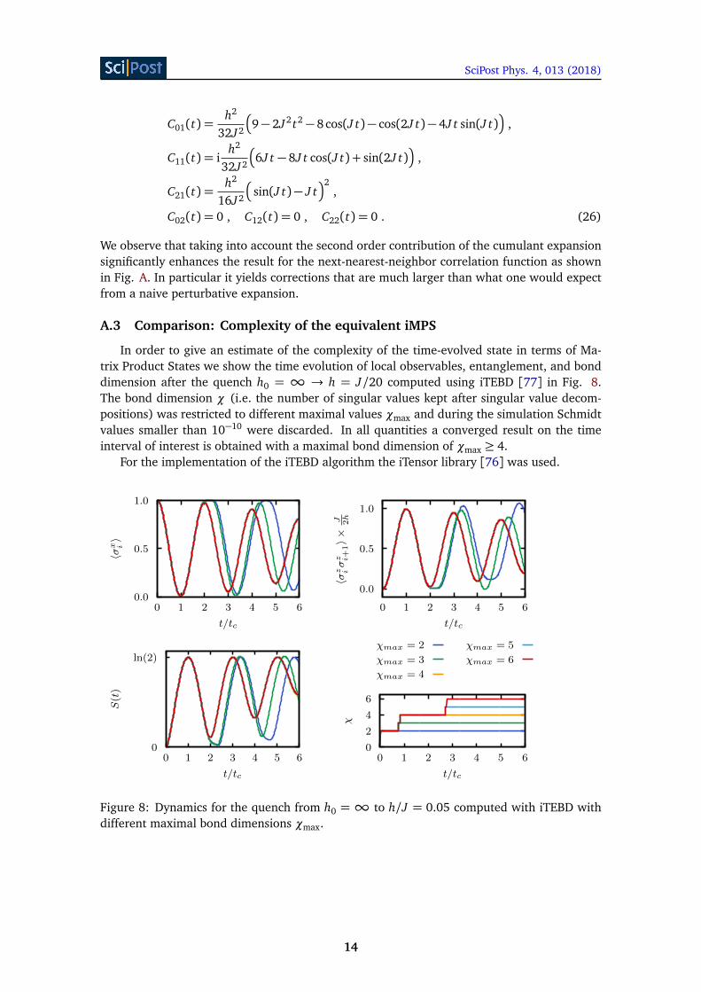
In order to give an estimate of the complexity of the time-evolved state in terms of Ma-trix Product States we show the time evolution of local observables, entanglement, and bonddimension after the quench h0 = ∞ → h = J/20 computed using iTEBD [77] in Fig. 8.The bond dimension χ (i.e. the number of singular values kept after singular value decom-positions) was restricted to different maximal values χmax and during the simulation Schmidtvalues smaller than 10−10 were discarded. In all quantities a converged result on the timeinterval of interest is obtained with a maximal bond dimension of χmax ≥ 4.

For the implementation of the iTEBD algorithm the iTensor library [76] was used.

0.0

0.5

1.0

0 1 2 3 4 5 6

0.0

0.5

1.0

0 1 2 3 4 5 6

0

ln(2)

0 1 2 3 4 5 60

2

4

6

0 1 2 3 4 5 6

〈σx i〉

t/tc

〈σz iσz i+

1〉×

J 2h

t/tc

S(t)

t/tc

χ

t/tc

χmax = 2

χmax = 3

χmax = 4

χmax = 5

χmax = 6

Figure 8: Dynamics for the quench from h0 =∞ to h/J = 0.05 computed with iTEBD withdifferent maximal bond dimensions χmax.

14

SciPost Phys. 4, 013 (2018)

B Loschmidt amplitude as classical partition function

B.1 Real weights from decimation RG

As outlined in the results section the Loschmidt amplitude (8) after integrating out every sec-ond spin, residing on sublattice Λ, can be integrated out, yielding

Z(t) =1

2N

∑

~s∈±1N/2

∏

i∈Λ2 cos

J4

t∑

⟨i, j⟩

s j

. (27)

A Hamilton function H (~s, t) defining a classical network can be obtained by choosing a gen-eral ansatz including all possible Z2-symmetric couplings of spins with a common neighboron the sublattice Λ, which takes the form given in Eq. (10). The Boltzmann weight of aconfiguration is then given by

eH (~s,t) =∏

l∈Λexp

z/2∑

n=0

Cn(t)∑

(a1,...,a2n)∈V l2n

2n∏

r=1

sar

. (28)

Equating each factor in the expression above with the corresponding factor in Eq. (27) forevery configuration of the involved spins yields a system of equations that determines thecouplings Cn(t) [65].

In d = 1 the couplings are

C0(t) = ln2+ln

cos(J t/2)

2, C1(t) =

ln

cos(J t/2)

2. (29)

The couplings in d = 2 are

C0(t) = ln 2+ln

cos(J t)

+ 4 ln

cos(J t/2)

8,

C1(t) =ln

cos(J t)

8,

C2(t) =ln

cos(J t)

− 4 ln

cos(J t/2)

8. (30)

In d = 3 the resulting couplings are

C0(t) = ln 2+ln

cos(3J t/2)

+ 6 ln

cos(J t)

+ 15 ln

cos(J t/2)

32,

C1(t) =ln

cos(3J t/2)

+ 2 ln

cos(J t)

− ln

cos(J t/2)

32,

C2(t) =ln

cos(3J t/2)

− 2 ln

cos(J t)

− ln

cos(J t/2)

32,

C3(t) =ln

cos(3J t/2)

− 6 ln

cos(J t)

+ 15 ln

cos(J t/2)

32. (31)

The time evolution of these couplings is displayed in Fig. 9.

15

SciPost Phys. 4, 013 (2018)

Re[ C

n(t)]

−3

−2

−1

0

1

2

3

C0(t) C1(t) C2(t) C3(t)

Im[ C

n(t)]

t/tc

−π

0

π

0 1 2

t/tc

0 12

1 32

2

t/tc

0 13

12

1 32

53

2

Figure 9: Time evolution of the couplings of the effective Hamilton function H (~s, t) for theLoschmidt amplitude in one, two, and three dimensions.

B.2 Monte-Carlo scheme for the Loschmidt amplitude

In order to evaluate the Loschmidt amplitude given in terms of the renormalized Boltz-mann weights (28) a combination of different Monte Carlo techniques is employed. Sincethe Loschmidt amplitude is the normalization of the Boltzmann weights a simple MetropolisMonte Carlo sampling is not sufficient. Moreover, the Monte Carlo sampling is hindered bycritical slowing down close to the critical times and the presence of negative weights leads toa sign problem.

The idea to deal with these issues is to sample for a given Hamilton function H (~s, t) theenergy histograms P±(E) = Ω±(E)eE where the density of statesΩ±(E) is the number of config-urations ~s with energy E = ReH (~s, t). The sign index indicates the sign of the correspondingBoltzmann weight. Given a good estimate of these histograms the partition sum is simply

Z(t) =∑

E,σ=±1

σ Pσ(E) . (32)

Note, however, that the histograms P±(E) must be properly normalized in order to get thecorrect result for Z(t). In order to obtain a good estimate of the normalized histogram wecombine the following techniques:

1. Separate sampling of factor graphs. In order to overcome the sign problem the configura-tion spaceX = ±1N

′is separated intoX+ = ~s|eH (~s,t) > 0 andX− = ~s|eH (~s,t) < 0;

N ′ is the number renormalized spins. Then the partition sum is split as

Z(t) = Z+(t) + Z−(t),

Z± =∑

~s∈X±

eH (~s,t) = ±∑

E

P±(E) . (33)

The partition sums Z± can be sampled separately as described in Ref. [67].

2. Importance sampling. When sampling the energy E in an importance sampling schemewith weights eE the relative frequency of samples with energy E is proportional toP±(E) = Ω±(E)eE . Therefore, a histogram of the energies sampled with MetropolisMonte Carlo updates yields the desired histograms up to normalization. Moreover, theimportance sampling allows to choose the region in the energy spectrum that is sampledby introducing an artificial temperature as described next.

16

SciPost Phys. 4, 013 (2018)

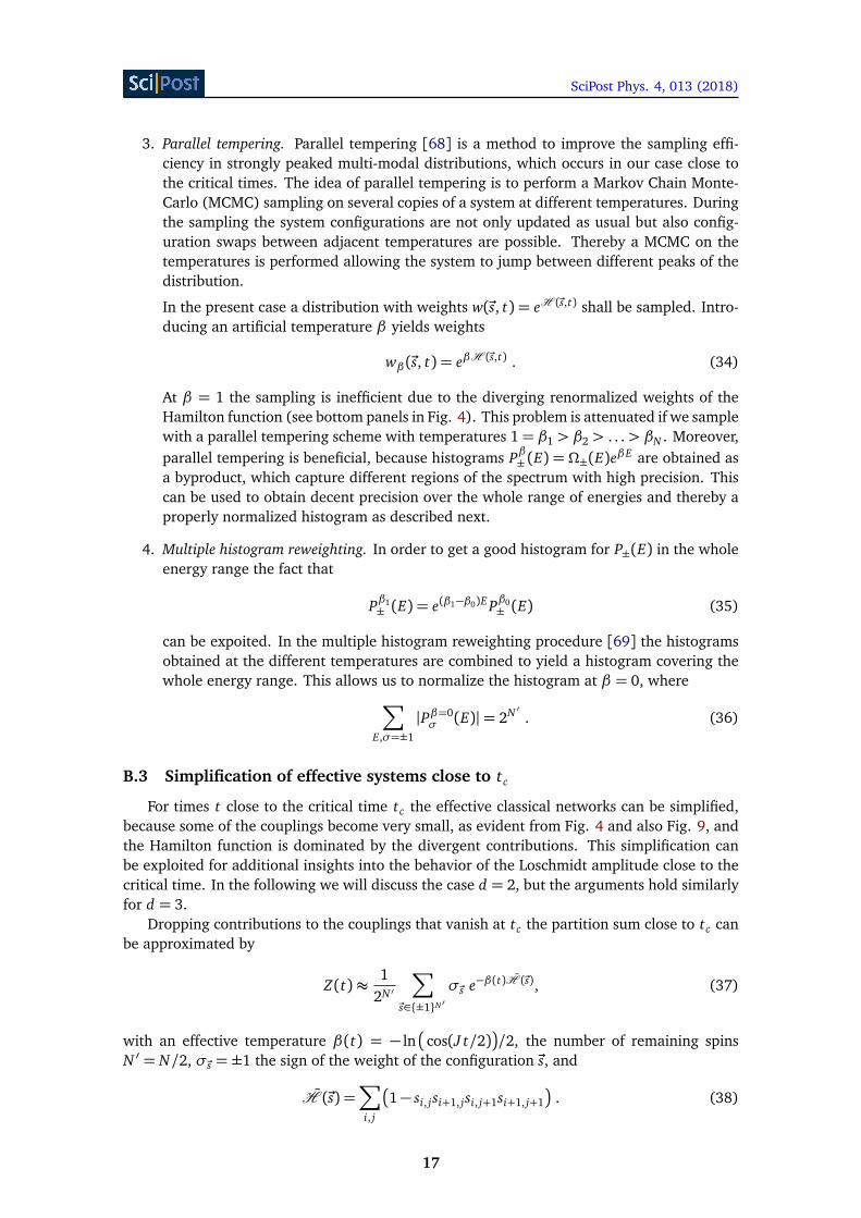
3. Parallel tempering. Parallel tempering [68] is a method to improve the sampling effi-ciency in strongly peaked multi-modal distributions, which occurs in our case close tothe critical times. The idea of parallel tempering is to perform a Markov Chain Monte-Carlo (MCMC) sampling on several copies of a system at different temperatures. Duringthe sampling the system configurations are not only updated as usual but also config-uration swaps between adjacent temperatures are possible. Thereby a MCMC on thetemperatures is performed allowing the system to jump between different peaks of thedistribution.

In the present case a distribution with weights w(~s, t) = eH (~s,t) shall be sampled. Intro-ducing an artificial temperature β yields weights

wβ(~s, t) = eβH (~s,t) . (34)

At β = 1 the sampling is inefficient due to the diverging renormalized weights of theHamilton function (see bottom panels in Fig. 4). This problem is attenuated if we samplewith a parallel tempering scheme with temperatures 1= β1 > β2 > . . .> βN . Moreover,parallel tempering is beneficial, because histograms Pβ± (E) = Ω±(E)e

βE are obtained asa byproduct, which capture different regions of the spectrum with high precision. Thiscan be used to obtain decent precision over the whole range of energies and thereby aproperly normalized histogram as described next.

4. Multiple histogram reweighting. In order to get a good histogram for P±(E) in the wholeenergy range the fact that

Pβ1± (E) = e(β1−β0)E Pβ0

± (E) (35)

can be expoited. In the multiple histogram reweighting procedure [69] the histogramsobtained at the different temperatures are combined to yield a histogram covering thewhole energy range. This allows us to normalize the histogram at β = 0, where

∑

E,σ=±1

|Pβ=0σ (E)|= 2N ′ . (36)

B.3 Simplification of effective systems close to tc

For times t close to the critical time tc the effective classical networks can be simplified,because some of the couplings become very small, as evident from Fig. 4 and also Fig. 9, andthe Hamilton function is dominated by the divergent contributions. This simplification canbe exploited for additional insights into the behavior of the Loschmidt amplitude close to thecritical time. In the following we will discuss the case d = 2, but the arguments hold similarlyfor d = 3.

Dropping contributions to the couplings that vanish at tc the partition sum close to tc canbe approximated by

Z(t)≈1

2N ′

∑

~s∈±1N ′σ~s e−β(t)H (~s), (37)

with an effective temperature β(t) = − ln

cos(J t/2)

/2, the number of remaining spinsN ′ = N/2, σ~s = ±1 the sign of the weight of the configuration ~s, and

H (~s) =∑

i, j

1− si, jsi+1, jsi, j+1si+1, j+1

. (38)

17

SciPost Phys. 4, 013 (2018)

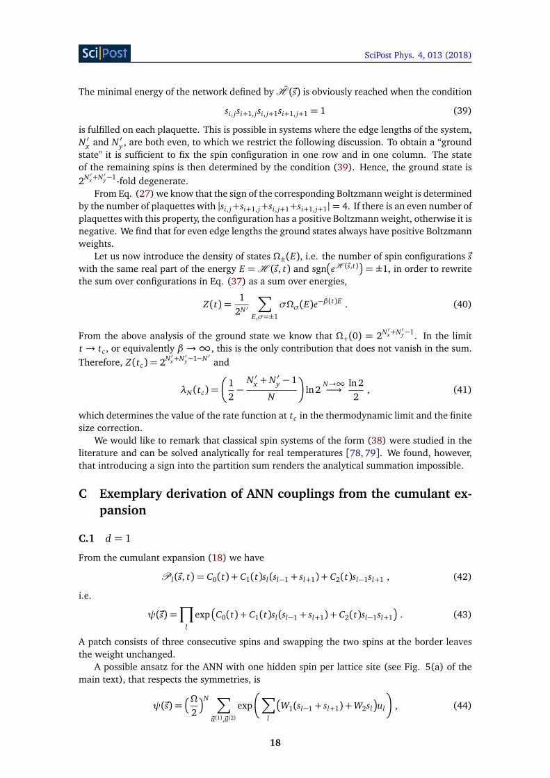
The minimal energy of the network defined by H (~s) is obviously reached when the condition

si, jsi+1, jsi, j+1si+1, j+1 = 1 (39)

is fulfilled on each plaquette. This is possible in systems where the edge lengths of the system,N ′x and N ′y , are both even, to which we restrict the following discussion. To obtain a “groundstate" it is sufficient to fix the spin configuration in one row and in one column. The stateof the remaining spins is then determined by the condition (39). Hence, the ground state is2N ′x+N ′y−1-fold degenerate.

From Eq. (27) we know that the sign of the corresponding Boltzmann weight is determinedby the number of plaquettes with |si, j+si+1, j+si, j+1+si+1, j+1|= 4. If there is an even number ofplaquettes with this property, the configuration has a positive Boltzmann weight, otherwise it isnegative. We find that for even edge lengths the ground states always have positive Boltzmannweights.

Let us now introduce the density of states Ω±(E), i.e. the number of spin configurations ~swith the same real part of the energy E =H (~s, t) and sgn

eH (~s,t)

= ±1, in order to rewritethe sum over configurations in Eq. (37) as a sum over energies,

Z(t) =1

2N ′

∑

E,σ=±1

σΩσ(E)e−β(t)E . (40)

From the above analysis of the ground state we know that Ω+(0) = 2N ′x+N ′y−1. In the limitt → tc , or equivalently β →∞, this is the only contribution that does not vanish in the sum.Therefore, Z(tc) = 2N ′x+N ′y−1−N ′ and

λN (tc) =

12−

N ′x + N ′y − 1

N

ln 2N→∞−→

ln 22

, (41)

which determines the value of the rate function at tc in the thermodynamic limit and the finitesize correction.

We would like to remark that classical spin systems of the form (38) were studied in theliterature and can be solved analytically for real temperatures [78, 79]. We found, however,that introducing a sign into the partition sum renders the analytical summation impossible.

C Exemplary derivation of ANN couplings from the cumulant ex-pansion

C.1 d = 1

From the cumulant expansion (18) we have

Pl(~s, t) = C0(t) + C1(t)sl(sl−1 + sl+1) + C2(t)sl−1sl+1 , (42)

i.e.

ψ(~s) =∏

l

exp

C0(t) + C1(t)sl(sl−1 + sl+1) + C2(t)sl−1sl+1

. (43)

A patch consists of three consecutive spins and swapping the two spins at the border leavesthe weight unchanged.

A possible ansatz for the ANN with one hidden spin per lattice site (see Fig. 5(a) of themain text), that respects the symmetries, is

ψ(~s) =Ω

2

N ∑

~u(1),~u(2)exp

∑

l

W1(sl−1 + sl+1) +W2sl

ul

, (44)

18

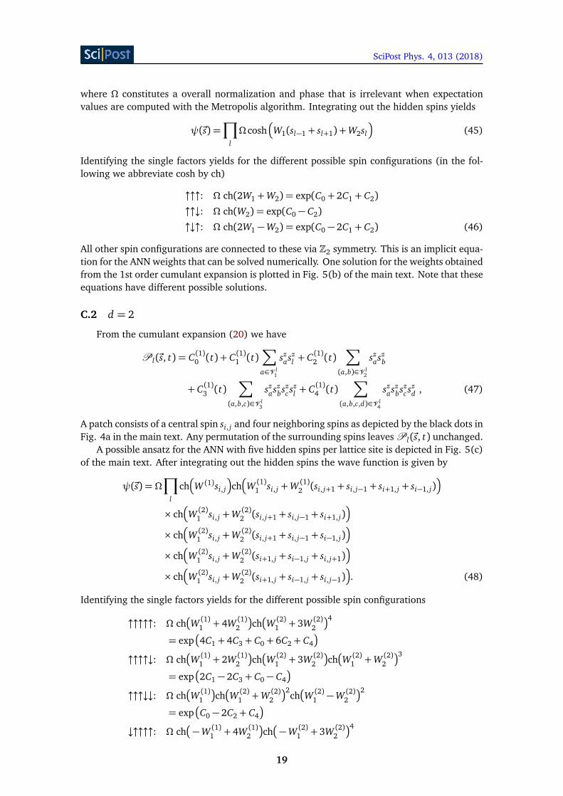
SciPost Phys. 4, 013 (2018)

where Ω constitutes a overall normalization and phase that is irrelevant when expectationvalues are computed with the Metropolis algorithm. Integrating out the hidden spins yields

ψ(~s) =∏

l

Ω cosh

W1(sl−1 + sl+1) +W2sl

(45)

Identifying the single factors yields for the different possible spin configurations (in the fol-lowing we abbreviate cosh by ch)

↑↑↑: Ω ch(2W1 +W2) = exp(C0 + 2C1 + C2)

↑↑↓: Ω ch(W2) = exp(C0 − C2)

↑↓↑: Ω ch(2W1 −W2) = exp(C0 − 2C1 + C2) (46)

All other spin configurations are connected to these via Z2 symmetry. This is an implicit equa-tion for the ANN weights that can be solved numerically. One solution for the weights obtainedfrom the 1st order cumulant expansion is plotted in Fig. 5(b) of the main text. Note that theseequations have different possible solutions.

C.2 d = 2

From the cumulant expansion (20) we have

Pl(~s, t) = C (1)0 (t) + C (1)1 (t)∑

a∈V l1

szasz

l + C (1)2 (t)∑

(a,b)∈V l2

szasz

b

+ C (1)3 (t)∑

(a,b,c)∈V l3

szasz

bszc sz

l + C (1)4 (t)∑

(a,b,c,d)∈V l4

szasz

bszc sz

d , (47)

A patch consists of a central spin si, j and four neighboring spins as depicted by the black dots inFig. 4a in the main text. Any permutation of the surrounding spins leaves Pl(~s, t) unchanged.

A possible ansatz for the ANN with five hidden spins per lattice site is depicted in Fig. 5(c)of the main text. After integrating out the hidden spins the wave function is given by

ψ(~s) = Ω∏

l

ch

W (1)si, j

ch

W (1)1 si, j +W (1)

2 (si, j+1 + si, j−1 + si+1, j + si−1, j)

× ch

W (2)1 si, j +W (2)

2 (si, j+1 + si, j−1 + si+1, j)

× ch

W (2)1 si, j +W (2)

2 (si, j+1 + si, j−1 + si−1, j)

× ch

W (2)1 si, j +W (2)

2 (si+1, j + si−1, j + si, j+1)

× ch

W (2)1 si, j +W (2)

2 (si+1, j + si−1, j + si, j−1)

. (48)

Identifying the single factors yields for the different possible spin configurations

↑↑↑↑↑: Ω ch

W (1)1 + 4W (1)

2

ch

W (2)1 + 3W (2)

2

4

= exp

4C1 + 4C3 + C0 + 6C2 + C4

↑↑↑↑↓: Ω ch

W (1)1 + 2W (1)

2

ch

W (2)1 + 3W (2)

2

ch

W (2)1 +W (2)

2

3

= exp

2C1 − 2C3 + C0 − C4

↑↑↑↓↓: Ω ch

W (1)1

ch

W (2)1 +W (2)

2

2ch

W (2)1 −W (2)

2

2

= exp

C0 − 2C2 + C4

↓↑↑↑↑: Ω ch

−W (1)1 + 4W (1)

2

ch

−W (2)1 + 3W (2)

2

4

19

SciPost Phys. 4, 013 (2018)

= exp

− 4C1 − 4C3 + C0 + 6C2 + C4

↓↑↑↑↓: Ω ch

−W (1)1 + 2W (1)

2

ch

−W (2)1 + 3W (2)

2

ch

−W (2)1 +W (2)

2

3

= exp

− 2C1 + 2C3 + C0 − C4

(49)

where the leftmost arrow in the spin configurations corresponds to the central spin of thepatch. One solution for the weights obtained from the 1st order cumulant expansion is plot-ted in Fig. 5(d) of the main text.

References

[1] S. R. White, Density matrix formulation for quantum renormalization groups, Phys. Rev.Lett. 69, 2863 (1992), doi:10.1103/PhysRevLett.69.2863.

[2] U. Schollwöck, The density-matrix renormalization group in the age of matrix productstates, Ann. Phys. 326, 96 (2011), doi:10.1016/j.aop.2010.09.012.

[3] R. Orús, A practical introduction to tensor networks: Matrix product states and projectedentangled pair states, Ann. Phys. 349, 117 (2014), doi:10.1016/j.aop.2014.06.013.

[4] A. Georges, G. Kotliar, W. Krauth and M. J. Rozenberg, Dynamical mean-field theory ofstrongly correlated fermion systems and the limit of infinite dimensions, Rev. Mod. Phys.68, 13 (1996), doi:10.1103/RevModPhys.68.13.

[5] D. Vollhardt, Dynamical mean-field theory for correlated electrons, Ann. Phys. 524, 1(2011), doi:10.1002/andp.201100250.

[6] J. K. Freericks, V. M. Turkowski and V. Zlatic, Nonequilibrium Dynamical Mean-Field The-ory, Phys. Rev. Lett. 97, 266408 (2006), doi:10.1103/PhysRevLett.97.266408.

[7] H. Aoki, N. Tsuji, M. Eckstein, M. Kollar, T. Oka and P. Werner, Nonequilibriumdynamical mean-field theory and its applications, Rev. Mod. Phys. 86, 779 (2014),doi:10.1103/RevModPhys.86.779.

[8] U. Schneider, L. Hackermuller, J. P. Ronzheimer, S. Will, S. Braun, T. Best, I. Bloch,E. Demler, S. Mandt, D. Rasch and A. Rosch, Fermionic transport and out-of-equilibriumdynamics in a homogeneous Hubbard model with ultracold atoms, Nat. Phys. 8, 213(2012), doi:10.1038/nphys2205.

[9] J.-y. Choi, S. Hild, J. Zeiher, P. Schauß, A. Rubio-Abadal, T. Yefsah, V. Khemani, D. A. Huse,I. Bloch and C. Gross, Exploring the many-body localization transition in two dimensions,Science 352, 1547 (2016), doi:10.1126/science.aaf8834.

[10] M. Mitrano, A. Cantaluppi, D. Nicoletti, S. Kaiser, A. Perucchi, S. Lupi, P. Di Pietro, D. Pon-tiroli, M. Riccò, S. R. Clark, D. Jaksch and A. Cavalleri, Possible light-induced superconduc-tivity in K3C60 at high temperature, Nature 530, 461 (2016), doi:10.1038/nature16522.

[11] N. Fläschner, D. Vogel, M. Tarnowski, B. Rem, D.-S. Lühmann, M. Heyl, H. Budich,L. Mathey, K. Sengstock and C. Weitenberg, Observation of dynamical vortices afterquenches in a system with topology, Nat. Phys. (2017), doi:10.1038/s41567-017-0013-8.

[12] S. Hild, T. Fukuhara, P. Schauß, J. Zeiher, M. Knap, E. Demler, I. Bloch and C. Gross, Far-from-Equilibrium Spin Transport in Heisenberg Quantum Magnets, Phys. Rev. Lett. 113,147205 (2014), doi:10.1103/PhysRevLett.113.147205.

20

SciPost Phys. 4, 013 (2018)

[13] P. Bordia, H. Lüschen, S. Scherg, S. Gopalakrishnan, M. Knap, U. Schneider and I. Bloch,Probing Slow Relaxation and Many-Body Localization in Two-Dimensional QuasiperiodicSystems, Phys. Rev. X 7, 041047 (2017), doi:10.1103/PhysRevX.7.041047.

[14] W. L. McMillan, Ground State of Liquid He4, Phys. Rev. 138, A442 (1965),doi:10.1103/PhysRev.138.A442.

[15] S. Sorella, Wave function optimization in the variational Monte Carlo method, Phys. Rev.B 71, 241103 (2005), doi:10.1103/PhysRevB.71.241103.

[16] M. Capello, F. Becca, M. Fabrizio and S. Sorella, Superfluid to Mott-InsulatorTransition in Bose-Hubbard Models, Phys. Rev. Lett. 99, 056402 (2007),doi:10.1103/PhysRevLett.99.056402.

[17] G. Carleo, F. Becca, M. Schiró and M. Fabrizio, Localization and Glassy Dynamics Of Many-Body Quantum Systems, Sci. Rep. 2, 243 (2012), doi:10.1038/srep00243.

[18] G. Carleo, F. Becca, L. Sanchez-Palencia, S. Sorella and M. Fabrizio, Light-cone effect andsupersonic correlations in one- and two-dimensional bosonic superfluids, Phys. Rev. A 89,031602 (2014), doi:10.1103/PhysRevA.89.031602.

[19] L. Cevolani, G. Carleo and L. Sanchez-Palencia, Protected quasilocality in quan-tum systems with long-range interactions, Phys. Rev. A 92, 041603 (2015),doi:10.1103/PhysRevA.92.041603.

[20] B. Blaß and H. Rieger, Test of quantum thermalization in the two-dimensional transverse-field Ising model, Scientific Reports 6, 38185 (2016), doi:10.1038/srep38185.

[21] J. Hafner, B. Blass and H. Rieger, Light cone in the two-dimensional transverse-field isingmodel in time-dependent mean-field theory, EPL 116, 60002 (2016), doi:10.1209/0295-5075/116/60002.

[22] G. Carleo, L. Cevolani, L. Sanchez-Palencia and M. Holzmann, Unitary Dynamics ofStrongly Interacting Bose Gases with the Time-Dependent Variational Monte Carlo Methodin Continuous Space, Phys. Rev. X 7, 031026 (2017), doi:10.1103/PhysRevX.7.031026.

[23] G. Carleo and M. Troyer, Solving the quantum many-body problem with artificial neuralnetworks, Science 355 (2017), doi:10.1126/science.aag2302.

[24] D.-L. Deng, X. Li and S. Das Sarma, Machine learning topological states, Phys. Rev. B 96,195145 (2017), doi:10.1103/PhysRevB.96.195145.

[25] D.-L. Deng, X. Li and S. Das Sarma, Quantum Entanglement in Neural Network States,Phys. Rev. X 7, 021021 (2017), doi:10.1103/PhysRevX.7.021021.

[26] Y. Huang and J. E. Moore, Neural network representation of tensor network and chiralstates, arXiv:1701.06246.

[27] J. Chen, S. Cheng, H. Xie, L. Wang and T. Xiang, Equivalence of restrictedBoltzmann machines and tensor network states, Phys. Rev. B 97, 085104 (2018),doi:10.1103/PhysRevB.97.085104.

[28] G. Torlai, G. Mazzola, J. Carrasquilla, M. Troyer, R. Melko and G. Carleo, Many-bodyquantum state tomography with neural networks, arXiv:1703.05334.

[29] Z. Cai and J. Liu, Approximating quantum many-body wave functions using artificial neuralnetworks, Phys. Rev. B 97, 035116 (2018), doi:10.1103/PhysRevB.97.035116.

21

SciPost Phys. 4, 013 (2018)

[30] X. Gao and L.-M. Duan, Efficient representation of quantum many-body states with deepneural networks, Nat. Commun. 8, 662 (2017), doi:10.1038/s41467-017-00705-2.

[31] R. Kaubruegger, L. Pastori and J. Carl Budich, Chiral Topological Phases from ArtificialNeural Networks, arXiv:1710.04713.

[32] H. Bernien, S. Schwartz, A. Keesling, H. Levine, A. Omran, H. Pichler, S. Choi, A. S.Zibrov, M. Endres, M. Greiner, V. Vuletic and M. D. Lukin, Probing many-body dynamicson a 51-atom quantum simulator, Nature 551, 579 (2017), doi:10.1038/nature24622.

[33] E. Guardado-Sanchez, P. T. Brown, D. Mitra, T. Devakul, D. A. Huse, P. Schauss and W. S.Bakr, Probing quench dynamics across a quantum phase transition into a 2D Ising antifer-romagnet, arXiv:1711.00887.

[34] P. Jurcevic et al., Direct Observation of Dynamical Quantum Phase Transitionsin an Interacting Many-Body System, Phys. Rev. Lett. 119, 080501 (2017),doi:10.1103/PhysRevLett.119.080501.

[35] E. Lieb, T. Schultz and D. Mattis, Two soluble models of an antiferromagnetic chain, Ann.Phys. 16, 407 (1961), doi:10.1016/0003-4916(61)90115-4.

[36] P. Pfeuty, The one-dimensional Ising model with a transverse field, Ann. Phys. 57, 79 (1970),doi:10.1016/0003-4916(70)90270-8.

[37] E. Barouch, B. M. McCoy and M. Dresden, Statistical mechanics of the XY model. i, Phys.Rev. A 2, 1075 (1970), doi:10.1103/PhysRevA.2.1075.

[38] E. Barouch and B. M. McCoy, Statistical mechanics of the x y model. ii. spin-correlationfunctions, Phys. Rev. A 3, 786 (1971), doi:10.1103/PhysRevA.3.786.

[39] E. Barouch and B. M. McCoy, Statistical mechanics of the XY model. iii, Phys. Rev. A 3,2137 (1971), doi:10.1103/PhysRevA.3.2137.

[40] F. Iglói and H. Rieger, Long-range correlations in the nonequilibrium quantum relaxationof a spin chain, Phys. Rev. Lett. 85, 3233 (2000), doi:10.1103/PhysRevLett.85.3233.

[41] K. Sengupta, S. Powell and S. Sachdev, Quench dynamics across quantum critical points,Phys. Rev. A 69, 053616 (2004), doi:10.1103/PhysRevA.69.053616.

[42] P. Calabrese, F. H. L. Essler and M. Fagotti, Quantum quench in the transverse field Isingchain: I. Time evolution of order parameter correlators, J. Stat. Mech.: Thoer. Exp. P07016(2012), doi:10.1088/1742-5468/2012/07/P07016.

[43] G. Vidal, J. I. Latorre, E. Rico and A. Kitaev, Entanglement in quantum critical phenomena,Phys. Rev. Lett. 90, 227902 (2002), doi:10.1103/PhysRevLett.90.227902

[44] J. I. Latorre, E. Rico and G. Vidal, Ground State Entanglement in Quantum Spin Chains,Quantum Info. Comput. 4, 48 (2004).

[45] M. Heyl, A. Polkovnikov and S. Kehrein, Dynamical Quantum Phase Transi-tions in the Transverse-Field Ising Model, Phys. Rev. Lett. 110, 135704 (2013),doi:10.1103/PhysRevLett.110.135704.

[46] M. Heyl, Dynamical quantum phase transitions: a review, arXiv:1709.07461.

22

SciPost Phys. 4, 013 (2018)

[47] F. Pollmann, S. Mukerjee, A. G. Green and J. E. Moore, Dynamics after asweep through a quantum critical point, Phys. Rev. E 81, 020101 (2010),doi:10.1103/PhysRevE.81.020101.

[48] C. Karrasch and D. Schuricht, Dynamical phase transitions after quenches in nonintegrablemodels, Phys. Rev. B 87, 195104 (2013), doi:10.1103/PhysRevB.87.195104.

[49] J. N. Kriel, C. Karrasch and S. Kehrein, Dynamical quantum phase transitionsin the axial next-nearest-neighbor Ising chain, Phys. Rev. B 90, 125106 (2014),doi:10.1103/PhysRevB.90.125106.

[50] A. J. A. James and R. M. Konik, Quantum quenches in two spatial dimen-sions using chain array matrix product states, Phys. Rev. B 92, 161111 (2015),doi:10.1103/PhysRevB.92.161111.

[51] M. Heyl, Scaling and Universality at Dynamical Quantum Phase Transitions, Phys. Rev.Lett. 115, 140602 (2015), doi:10.1103/PhysRevLett.115.140602.

[52] N. O. Abeling and S. Kehrein, Quantum quench dynamics in the transversefield Ising model at nonzero temperatures, Phys. Rev. B 93, 104302 (2016),doi:10.1103/PhysRevB.93.104302.

[53] S. Sharma, U. Divakaran, A. Polkovnikov and A. Dutta, Slow quenches in a quantumIsing chain: Dynamical phase transitions and topology, Phys. Rev. B 93, 144306 (2016),doi:10.1103/PhysRevB.93.144306.

[54] B. Zunkovic, M. Heyl, M. Knap and A. Silva, Dynamical Quantum Phase Transitions inSpin Chains with Long-Range Interactions: Merging different concepts of non-equilibriumcriticality, arXiv:1609.08482.

[55] J. C. Halimeh and V. Zauner-Stauber, Dynamical phase diagram of quantumspin chains with long-range interactions, Phys. Rev. B 96, 134427 (2017),doi:10.1103/PhysRevB.96.134427.

[56] M. Heyl, Quenching a quantum critical state by the order parameter: Dynamical quan-tum phase transitions and quantum speed limits, Phys. Rev. B 95, 060504 (2017),doi:10.1103/PhysRevB.95.060504.

[57] I. Homrighausen, N. O. Abeling, V. Zauner-Stauber and J. C. Halimeh, Anomalous dynam-ical phase in quantum spin chains with long-range interactions, Phys. Rev. B 96, 104436(2017), doi:10.1103/PhysRevB.96.104436.

[58] R. Kubo, Generalized Cumulant Expansion Method, J. Phys. Soc. Jpn. 17, 1100 (1962),doi:10.1143/JPSJ.17.1100.

[59] P. A. M. Dirac, Note on Exchange Phenomena in the Thomas Atom, Math. Proc. Camb. Phil.Soc. 26, 376 (1930), doi:10.1017/S0305004100016108.

[60] R. Jackiw and A. Kerman, Time-dependent variational principle and the effective action,Phys. Lett. A 71, 158 (1979), doi:10.1016/0375-9601(79)90151-8.

[61] J. Haegeman, J. I. Cirac, T. J. Osborne, I. Pižorn, H. Verschelde and F. Verstraete,Time-Dependent Variational Principle for Quantum Lattices, Phys. Rev. Lett. 107, 070601(2011), doi:10.1103/PhysRevLett.107.070601.

23

SciPost Phys. 4, 013 (2018)

[62] N. Metropolis, A. W. Rosenbluth, M. N. Rosenbluth, A. H. Teller and E. Teller, Equa-tion of State Calculations by Fast Computing Machines, J. Chem. Phys. 21, 1087 (1953),doi:10.1063/1.1699114.

[63] M. B. Hastings, I. González, A. B. Kallin and R. G. Melko, Measuring Renyi Entangle-ment Entropy in Quantum Monte Carlo Simulations, Phys. Rev. Lett. 104, 157201 (2010),doi:10.1103/PhysRevLett.104.157201.

[64] E. Martinez, C. Muschik, P. Schindler, D. Nigg, A. Erhard, M. Heyl, P. Hauke, M. Dalmonte,T. Monz, P. Zoller and R. Blatt, Real-time dynamics of lattice gauge theories with a few-qubitquantum computer, nature 534, 516 (2016), doi:10.1038/nature18318.

[65] B. Hu, Introduction to real-space renormalization-group methods in critical and chaoticphenomena, Phys. Rep. 91, 233 (1982), doi:10.1016/0370-1573(82)90057-6.

[66] J. F. Markham and T. D. Kieu, Simulations with complex measure, Nucl. Phys. B 516, 729(1998), doi:10.1016/S0550-3213(97)00831-6.

[67] M. Molkaraie and H.-A. Loeliger, Extending monte carlo methods to factor graphs withnegative and complex factors, Proc. 2012 IEEE Information Theory Workshop, 367 (2012),doi:10.1109/ITW.2012.6404694.

[68] D. J. Earl and M. W. Deem, Parallel tempering: Theory, applications, and new perspectives,Phys. Chem. Chem. Phys. 7, 3910 (2005), doi:10.1039/B509983H.

[69] A. M. Ferrenberg and R. H. Swendsen, Optimized Monte Carlo data analysis, Phys. Rev.Lett. 63, 1195 (1989), doi:10.1103/PhysRevLett.63.1195.

[70] S. Sachdev, Quantum Phase Transitions, Cambridge University Press, Cambridge (2011).

[71] R. Nandkishore and D. A. Huse, Many-Body Localization and Thermalization inQuantum Statistical Mechanics, Annu. Rev. Condens. Matter Phys. 6, 15 (2015),doi:10.1146/annurev-conmatphys-031214-014726.

[72] E. Altman and R. Vosk, Universal Dynamics and Renormalization in Many-Body-LocalizedSystems, Annu. Rev. Condens. Matter Phys. 6, 383 (2015), doi:10.1146/annurev-conmatphys-031214-014701.

[73] M. Schreiber, S. S. Hodgman, P. Bordia, H. P. Lüschen, M. H. Fischer, R. Vosk, E. Altman,U. Schneider and I. Bloch, Observation of many-body localization of interacting fermionsin a quasirandom optical lattice, Science 349, 842 (2015), doi:10.1126/science.aaa7432.

[74] J. Smith, A. Lee, P. Richerme, B. Neyenhuis, P. W. Hess, P. Hauke, M. Heyl, D. A. Huse andC. Monroe, Many-body localization in a quantum simulator with programmable randomdisorder, Nat. Phys. 12, 907 (2016), doi:10.1038/nphys3783.

[75] C. Sanderson and R. Curtin, Armadillo: a template-based C++ library for linear algebra,JOSS 1, 26 (2016), doi:10.21105/joss.00026.

[76] http://itensor.org/, version 2.1.0.

[77] J. A. Kjäll, M. P. Zaletel, R. S. K. Mong, J. H. Bardarson and F. Pollmann, Phase diagramof the anisotropic spin-2 XXZ model: Infinite-system density matrix renormalization groupstudy, Phys. Rev. B 87, 235106 (2013), doi:10.1103/PhysRevB.87.235106.

[78] M. Suzuki, Solution and Critical Behavior of Some "Three-Dimensional" Ising Models with aFour-Spin Interaction, Phys. Rev. Lett. 28, 507 (1972), doi:10.1103/PhysRevLett.28.507.

24

SciPost Phys. 4, 013 (2018)

[79] M. Mueller, D. A. Johnston and W. Janke, Exact solutions to plaquette Isingmodels with free and periodic boundaries, Nucl. Phys. B 914, 388 (2017),doi:10.1016/j.nuclphysb.2016.11.005.

25