Embed Size (px)
Citation preview
The Annals of Probability2016, Vol. 44, No. 6, 3804–3848DOI: 10.1214/15-AOP1061© Institute of Mathematical Statistics, 2016
QUANTUM GRAVITY AND INVENTORY ACCUMULATION
BY SCOTT SHEFFIELD
Massachusetts Institute of Technology
We begin by studying inventory accumulation at a LIFO (last-in-first-out) retailer with two products. In the simplest version, the following occurwith equal probability at each time step: first product ordered, first productproduced, second product ordered, second product produced. The inventorythus evolves as a simple random walk on Z2. In more interesting versions,a p fraction of customers orders the “freshest available” product regardlessof type. We show that the corresponding random walks scale to Brownianmotions with diffusion matrices depending on p.
We then turn our attention to the critical Fortuin–Kastelyn random pla-nar map model, which gives, for each q > 0, a probability measure on ran-dom (discretized) two-dimensional surfaces decorated by loops, related tothe q-state Potts model. A longstanding open problem is to show that asthe discretization gets finer, the surfaces converge in law to a limiting (loop-decorated) random surface. The limit is expected to be a Liouville quantumgravity surface decorated by a conformal loop ensemble, with parameters de-pending on q. Thanks to a bijection between decorated planar maps and in-ventory trajectories (closely related to bijections of Bernardi and Mullin), ourresults about the latter imply convergence of the former in a particular topol-ogy. A phase transition occurs at p = 1/2, q = 4.
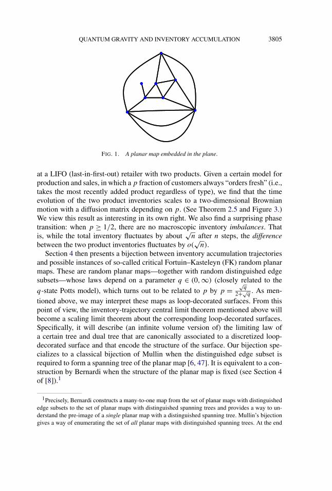
1. Introduction. A planar map is a connected planar graph together with anembedding into the sphere (which we identify with the complex plane C∪ {∞}),defined up to topological deformation. Self loops and multi-edges are allowed. SeeFigure 1.
There is a significant literature on random planar maps of various types. As weillustrate later, planar maps are in one-to-one correspondence with planar quad-rangulations, which in turn can be interpreted as Riemannian surfaces, obtainedby gluing together unit squares along their boundaries (see Figure 6). If we alsodeclare a random subset of the edges of a planar map to be “open”, we can gen-erate a set of loops on the Riemannian surface that separate open clusters fromdual clusters (see Figures 7 and 9). We are interested in the “scaling limits” ofthese random loop-decorated surfaces when the number of unit squares tends toinfinity.
However, we approach the problem from an unconventional direction. We beginin Sections 2 and 3 by stating and proving a theorem about inventory accumulation
Received June 2014; revised September 2015.MSC2010 subject classifications. 60K35, 60D05.Key words and phrases. Liouville quantum gravity, planar map, scaling limit, Schramm–Loewner
evolution, FK random cluster model, continuum random tree, mating of trees.
3804
QUANTUM GRAVITY AND INVENTORY ACCUMULATION 3805
FIG. 1. A planar map embedded in the plane.
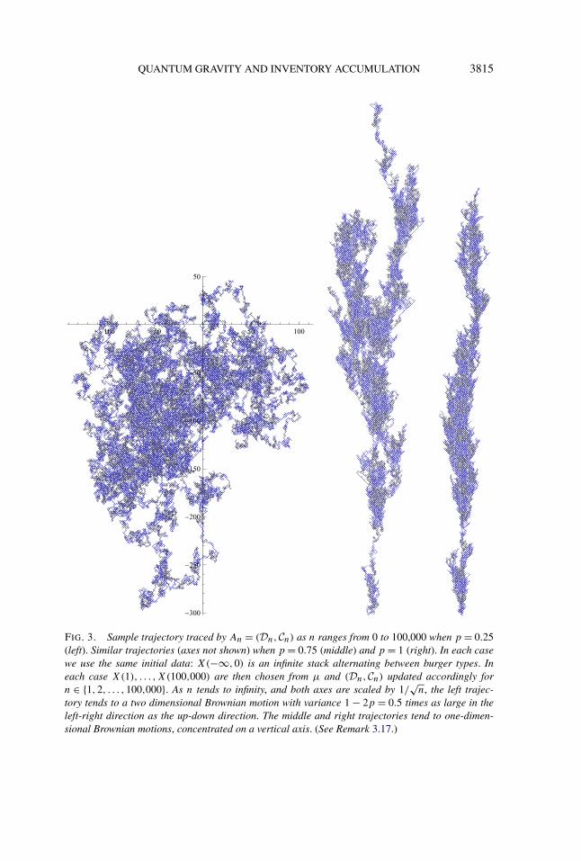
at a LIFO (last-in-first-out) retailer with two products. Given a certain model forproduction and sales, in which a p fraction of customers always “orders fresh” (i.e.,takes the most recently added product regardless of type), we find that the timeevolution of the two product inventories scales to a two-dimensional Brownianmotion with a diffusion matrix depending on p. (See Theorem 2.5 and Figure 3.)We view this result as interesting in its own right. We also find a surprising phasetransition: when p ≥ 1/2, there are no macroscopic inventory imbalances. Thatis, while the total inventory fluctuates by about
√n after n steps, the difference
between the two product inventories fluctuates by o(√
n).Section 4 then presents a bijection between inventory accumulation trajectories
and possible instances of so-called critical Fortuin–Kasteleyn (FK) random planarmaps. These are random planar maps—together with random distinguished edgesubsets—whose laws depend on a parameter q ∈ (0,∞) (closely related to the
q-state Potts model), which turns out to be related to p by p =√
q
2+√q
. As men-tioned above, we may interpret these maps as loop-decorated surfaces. From thispoint of view, the inventory-trajectory central limit theorem mentioned above willbecome a scaling limit theorem about the corresponding loop-decorated surfaces.Specifically, it will describe (an infinite volume version of) the limiting law ofa certain tree and dual tree that are canonically associated to a discretized loop-decorated surface and that encode the structure of the surface. Our bijection spe-cializes to a classical bijection of Mullin when the distinguished edge subset isrequired to form a spanning tree of the planar map [6, 47]. It is equivalent to a con-struction by Bernardi when the structure of the planar map is fixed (see Section 4of [8]).1
1Precisely, Bernardi constructs a many-to-one map from the set of planar maps with distinguishededge subsets to the set of planar maps with distinguished spanning trees and provides a way to un-derstand the pre-image of a single planar map with a distinguished spanning tree. Mullin’s bijectiongives a way of enumerating the set of all planar maps with distinguished spanning trees. At the end
3806 S. SHEFFIELD
The proofs in this paper are discrete and elementary, relying only on standardresults in probability (such as the optional stopping theorem). We remark, however,that we view this paper as part of a larger program to relate random planar maps tocontinuum objects such as Liouville quantum gravity and the Schramm–Loewnerevolution. We will not discuss these ideas in the body of the paper, but we providea brief explanation of this point of view in an Appendix. Let us note that sincethis paper was first posted to the arXiv, there have been many additional papersthat have used the theory developed here to prove the convergence the randomplanar map models to continuum models (involving conformal loop ensemblesand Liouville quantum gravity) in certain topologies [19, 27–30, 46]. Other workshave described tail exponents of the planar map models [5], a generalization tomore than two burger types [42], a further study of the infinite critical-FK randommap [12], and a related sandpile result [55].
We also remark that there is a vast operations research literature on inven-tory management protocols, including various schemes involving two products,but to our knowledge this is the first paper to address this particular model, andalso the first to make the connection between inventory trajectories and planarmaps.
2. Inventory trajectories: Setup and theorem statement. In this section,we describe a random walk on a particular semi-group (related, as we will see inSection 4, to random planar maps) and study its scaling limit. We interpret thewalk as a simple model for inventory accumulation at a LIFO (last-in-first-out)retailer with two product types and three order types (first product, second prod-uct, and “flexible”/“freshest available”) arriving at random times. As a convenientmnemonic, we refer to the two products as hamburgers and cheeseburgers (orburgers collectively).2
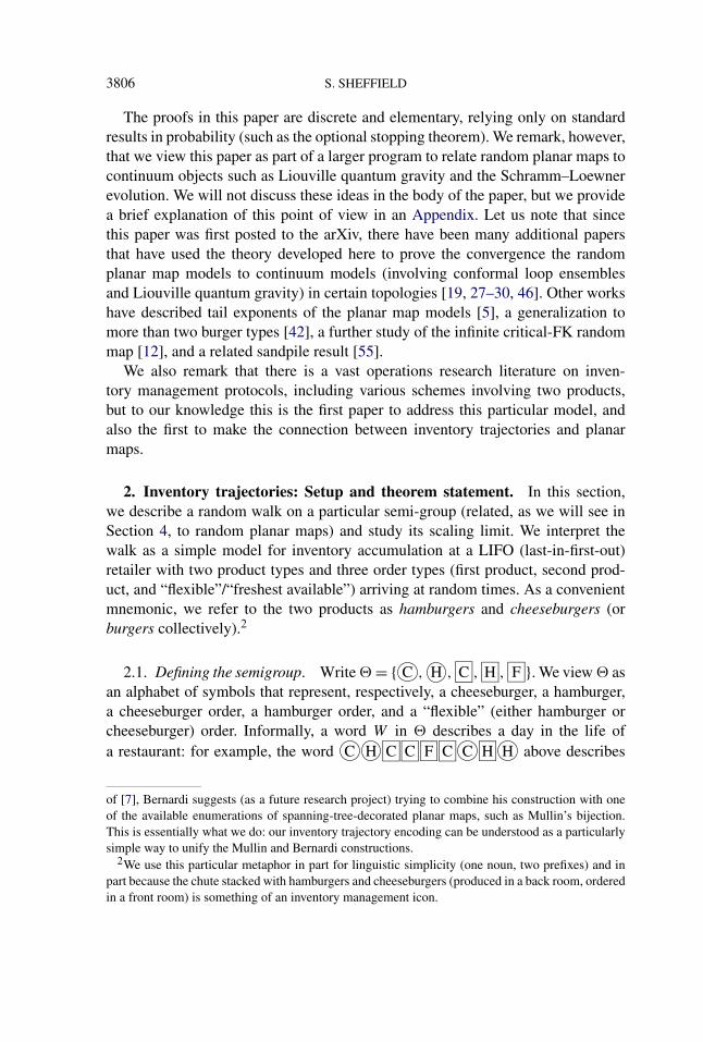
2.1. Defining the semigroup. Write � = { C , H , C , H , F }. We view � asan alphabet of symbols that represent, respectively, a cheeseburger, a hamburger,a cheeseburger order, a hamburger order, and a “flexible” (either hamburger orcheeseburger) order. Informally, a word W in � describes a day in the life ofa restaurant: for example, the word C H C C F C C H H above describes
of [7], Bernardi suggests (as a future research project) trying to combine his construction with oneof the available enumerations of spanning-tree-decorated planar maps, such as Mullin’s bijection.This is essentially what we do: our inventory trajectory encoding can be understood as a particularlysimple way to unify the Mullin and Bernardi constructions.
2We use this particular metaphor in part for linguistic simplicity (one noun, two prefixes) and inpart because the chute stacked with hamburgers and cheeseburgers (produced in a back room, orderedin a front room) is something of an inventory management icon.
QUANTUM GRAVITY AND INVENTORY ACCUMULATION 3807
a day in which first someone produced a cheeseburger (to put on the top of a“stack” of burgers), then someone produced a hamburger, then two people orderedcheeseburgers, one ordered “freshest available,” another ordered a cheeseburger,someone produced a cheeseburger, someone ordered a hamburger, and someoneproduced a hamburger. Informally, we say that whenever a burger is produced, itis added to the top of the stack, and whenever an order is placed it is fulfilled (ifpossible) by removing the highest matching burger from the stack (but an order thatcannot be filled immediately remains unfilled—because the impatient customerleaves the restaurant, say).
To describe this formally, we view the elements of � as generators for a certain(associative) semigroup G, each element of which can be represented by a word W
in the alphabet � (with the empty string ∅ as a left and right identity). This is thesemigroup of words modulo four “order fulfillment” relations
C C = H H = C F = H F =∅,
and two “commutativity” relations
C H = H C ,
H C = C H .
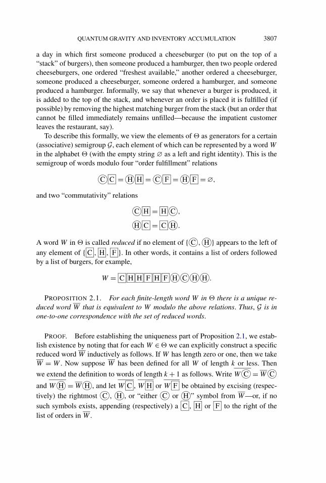
A word W in � is called reduced if no element of { C , H } appears to the left ofany element of { C , H , F }. In other words, it contains a list of orders followedby a list of burgers, for example,
W = C H H F H F H C H H .
PROPOSITION 2.1. For each finite-length word W in � there is a unique re-duced word W that is equivalent to W modulo the above relations. Thus, G is inone-to-one correspondence with the set of reduced words.
PROOF. Before establishing the uniqueness part of Proposition 2.1, we estab-lish existence by noting that for each W ∈ � we can explicitly construct a specificreduced word W inductively as follows. If W has length zero or one, then we takeW = W . Now suppose W has been defined for all W of length k or less. Then
we extend the definition to words of length k + 1 as follows. Write W C = W C
and W H = W H , and let W C , W H or W F be obtained by excising (respec-tively) the rightmost C , H , or “either C or H ” symbol from W—or, if nosuch symbols exists, appending (respectively) a C , H or F to the right of thelist of orders in W .
3808 S. SHEFFIELD
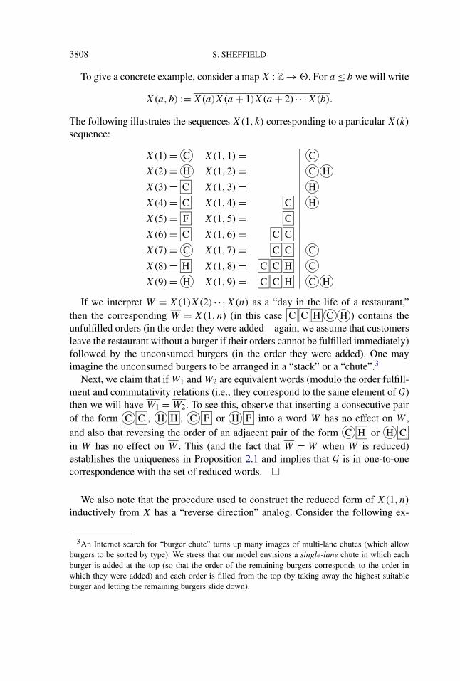
To give a concrete example, consider a map X : Z → �. For a ≤ b we will write
X(a, b) := X(a)X(a + 1)X(a + 2) · · ·X(b).
The following illustrates the sequences X(1, k) corresponding to a particular X(k)
sequence:
X(1) = C X(1,1) = C
X(2) = H X(1,2) = C H
X(3) = C X(1,3) = H
X(4) = C X(1,4) = C H
X(5) = F X(1,5) = C
X(6) = C X(1,6) = C C
X(7) = C X(1,7) = C C C
X(8) = H X(1,8) = C C H C
X(9) = H X(1,9) = C C H C H
If we interpret W = X(1)X(2) · · ·X(n) as a “day in the life of a restaurant,”then the corresponding W = X(1, n) (in this case C C H C H ) contains theunfulfilled orders (in the order they were added—again, we assume that customersleave the restaurant without a burger if their orders cannot be fulfilled immediately)followed by the unconsumed burgers (in the order they were added). One mayimagine the unconsumed burgers to be arranged in a “stack” or a “chute”.3
Next, we claim that if W1 and W2 are equivalent words (modulo the order fulfill-ment and commutativity relations (i.e., they correspond to the same element of G)then we will have W1 = W2. To see this, observe that inserting a consecutive pairof the form C C , H H , C F or H F into a word W has no effect on W ,
and also that reversing the order of an adjacent pair of the form C H or H Cin W has no effect on W . This (and the fact that W = W when W is reduced)establishes the uniqueness in Proposition 2.1 and implies that G is in one-to-onecorrespondence with the set of reduced words. �
We also note that the procedure used to construct the reduced form of X(1, n)
inductively from X has a “reverse direction” analog. Consider the following ex-
3An Internet search for “burger chute” turns up many images of multi-lane chutes (which allowburgers to be sorted by type). We stress that our model envisions a single-lane chute in which eachburger is added at the top (so that the order of the remaining burgers corresponds to the order inwhich they were added) and each order is filled from the top (by taking away the highest suitableburger and letting the remaining burgers slide down).
QUANTUM GRAVITY AND INVENTORY ACCUMULATION 3809
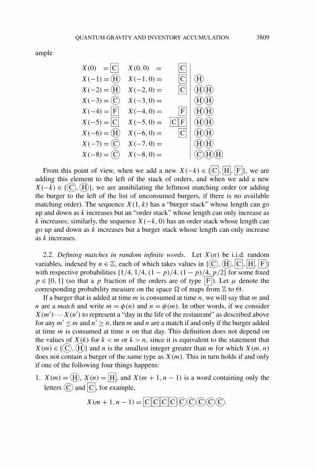
ample
X(0) = C X(0,0) = C
X(−1) = H X(−1,0) = C H
X(−2) = H X(−2,0) = C H H
X(−3) = C X(−3,0) = H H
X(−4) = F X(−4,0) = F H H
X(−5) = C X(−5,0) = C F H H
X(−6) = H X(−6,0) = C H H
X(−7) = C X(−7,0) = H H
X(−8) = C X(−8,0) = C H H
From this point of view, when we add a new X(−k) ∈ { C , H , F }, we areadding this element to the left of the stack of orders, and when we add a newX(−k) ∈ { C , H }, we are annihilating the leftmost matching order (or addingthe burger to the left of the list of unconsumed burgers, if there is no availablematching order). The sequence X(1, k) has a “burger stack” whose length can goup and down as k increases but an “order stack” whose length can only increase ask increases; similarly, the sequence X(−k,0) has an order stack whose length cango up and down as k increases but a burger stack whose length can only increaseas k increases.
2.2. Defining matches in random infinite words. Let X(n) be i.i.d. randomvariables, indexed by n ∈ Z, each of which takes values in { C , H , C , H , F }with respective probabilities {1/4,1/4, (1 − p)/4, (1 − p)/4,p/2} for some fixedp ∈ [0,1] (so that a p fraction of the orders are of type F ). Let μ denote thecorresponding probability measure on the space � of maps from Z to �.
If a burger that is added at time m is consumed at time n, we will say that m andn are a match and write m = φ(n) and n = φ(m). In other words, if we considerX(m′) · · ·X(n′) to represent a “day in the life of the restaurant” as described abovefor any m′ ≤ m and n′ ≥ n, then m and n are a match if and only if the burger addedat time m is consumed at time n on that day. This definition does not depend onthe values of X(k) for k < m or k > n, since it is equivalent to the statement thatX(m) ∈ { C , H } and n is the smallest integer greater than m for which X(m,n)
does not contain a burger of the same type as X(m). This in turn holds if and onlyif one of the following four things happens:
1. X(m) = H , X(n) = H , and X(m + 1, n − 1) is a word containing only theletters C and C , for example,
X(m + 1, n − 1) = C C C C C C C C C .
3810 S. SHEFFIELD
2. X(m) = C , X(n) = C , and X(m + 1, n − 1) is a word containing only theletters H and H , for example,
X(m + 1, n − 1) = H H H H H H H .
3. X(m) = H , X(n) = F and X(m + 1, n − 1) is a word containing only theletter C , for example,
X(m + 1, n − 1) = C C C C .
4. X(m) = C , X(n) = F and X(m + 1, n − 1) is a word containing only theletter H , for example,
X(m + 1, n − 1) = H H H H H H H H .
If X(m) ∈ { C , H } and m has no match [i.e., the burger added at time m
is never consumed—which would be the case, for example, if we had X(k) ∈{ C , H } for all k > m]—we write φ(m) = ∞. If X(n) ∈ { C , H , F } and n hasno match (i.e., the order at time n is unfulfilled, no matter how far back in time onestarts), then we write φ(n) = −∞.
For example, in the sequence
X(1) = C X(1,1) = C
X(2) = H X(1,2) = C H
X(3) = C X(1,3) = H
X(4) = C X(1,4) = C H
X(5) = F X(1,5) = C
X(6) = C X(1,6) = C C
X(7) = C X(1,7) = C C C
X(8) = H X(1,8) = C C H C
X(9) = H X(1,9) = C C H C H
described above, we have φ(3) = 1; φ(1) = 3 and φ(2) = 5; φ(5) = 2, but the val-ues of φ(4), φ(6), φ(7), φ(8), φ(9) necessarily lie outside the interval {1,2, . . . ,9}and are not determined by X(1),X(2), . . . ,X(9).
PROPOSITION 2.2. It is μ almost surely the case that for every m ∈ Z, wehave φ(m) /∈ {−∞,∞}. In other words, every X(j) has a unique match, almostsurely, so that φ is an involution on Z.
PROOF. We first claim that this holds whenever X(m) ∈ { C , H }. Observethat the net number of burgers (i.e., the number of burger symbols minus the num-ber of order symbols) added between times m and n, as a function of n, is a simple

QUANTUM GRAVITY AND INVENTORY ACCUMULATION 3811
random walk on Z. It follows that there will almost surely exist values of n > m forwhich this quantity is arbitrarily negative, and hence X(m + 1, n) contains an ar-bitrarily long sequence of orders. [Recall that the number of orders in X(m+ 1, n)
is nondecreasing as n increases.] If X(m) = C , then the first time that a C orF is added to this list of orders will be a time at which X(m) is consumed; thus,
on the event that m has no match it is almost surely the case that the number of Horders in X(m + 1, n) tends to infinity as n → ∞ while the number of C ordersremains zero. If this happens for some m, then there cannot be an m′ for whichthe same thing happens with the roles of hamburgers and cheeseburgers reversed[since X(m + 1,m′) is a fixed finite length word—appending it on the left can-not remove an arbitrarily long sequence of C elements from the correspondingreduced word]. Thus, it is almost surely the case that either every cheeseburgeradded (at any integer time) is ultimately consumed or every hamburger added (atany integer time) is ultimately consumed. Since each of these two events is trans-lation invariant, the zero-one law for translation invariant events (see any textbookwith an introduction to ergodic decompositions, e.g., [25]) implies that each hasprobability zero or probability one. As observed above, the union of these twoevents has probability one, so by symmetry each of them separately has μ proba-bility one. Thus, μ a.s. every burger of either type is ultimately consumed, whichimplies the claim. A similar argument (in the reverse direction) shows that φ(n) isa.s. finite whenever X(n) ∈ { C , H , F }. �
The following is an immediate consequence of the above construction.
PROPOSITION 2.3. The reduced word X(1, n) contains precisely those X(k)
corresponding to the k ∈ {1,2, . . . , n} for which φ(k) /∈ {1,2, . . . , n}. In otherwords, it contains the list of unmatched orders [in order of appearance in the se-quence X(1),X(2), . . . ,X(n)] followed by the ordered list of unmatched burgers[in order of appearance in X(1),X(2), . . . ,X(n)].
2.3. Infinite stacks and random walks: Main theorem. By analogy with Propo-sition 2.3, we define X(−∞, n) to be the ordered sequence of X(k) for whichk ≤ n but φ(k) > n. Informally, we can write
X(−∞, n) = · · ·X(−3)X(−2)X(−1)X(0)X(1)X(2) · · ·X(n),
and interpret X(−∞, n) as the reduced form word corresponding to the productof all X(k) with k ≤ n. We view X(−∞, n) as a semi-infinite stack of C andH symbols, indexed by the negative integers; it has a unique top element but no
bottom element. [The number of elements in X(−∞, n) is μ a.s. infinite for all n
by Proposition 2.2—if it were some finite value k, then with positive probabilitythere would be a consecutive sequence of k + 1 orders after time n, and at leastone order would have no match.]
3812 S. SHEFFIELD
We similarly write
X(n,∞) := X(n)X(n + 1), . . . ,
which we interpret to mean the ordered sequence of X(k) for which k ≥ n butφ(k) < n. It is natural to represent X(n,∞) as a sequence of { C , H , F } val-ues indexed by the positive integers. While the X(−∞, n) can be interpreted asa semi-infinite stack of burgers waiting to be consumed (as n increases in time),the stack X(n,∞) can be interpreted as a semi-infinite queue of customers wait-ing to be served (as n decreases in time). A useful equivalent definition is thatX(n,∞) is the limit of the order stacks of X(n,m) (which only increase in lengthas m increases, with new orders being added on the right), as m → ∞. Similarly,X(−∞, n) is the limit of the burger stacks of X(m,n) (which only increase inlength as m decreases, with new burgers being added on the left) as m → −∞.
Next, define
Y(n) :=
⎧⎪⎪⎨⎪⎪⎩
X(n), X(n) ∈ {C , H , C , H
},
C , X(n) = F , X(φ(n)
) = C ,
H , X(n) = F , X(φ(n)
) = H .
In other words, Y(n) is obtained from X(n) by replacing each F with a C orH , depending on which burger type was actually consumed by the F order. Fora ≤ b, we also write
Y(a, b) := Y(a)Y (a + 1) · · ·Y(b),
and observe that this is the same as X(a, b) except that each F is replaced withthe corresponding C or H symbol.
For every word W in the symbols { C , H , C , H , F }, we write C(W) forthe net burger count (i.e., the number of { C , H } symbols minus the numberof { C , H , F } symbols in W ). Analogously, if W has no F symbols, then wedefine D(W) to be the net discrepancy of hamburgers over cheeseburgers (i.e., thenumber of { H , C } symbols minus the number of { C , H } symbols).
DEFINITION 2.4. Given the infinite X(n) sequence, let Cn be the integer val-ued process defined by C0 = 0 and Cn − Cn−1 = C(Y (n)) for all n. Similarly,write D0 = 0 and Dn − Dn−1 = D(Y (n)). Thus, Cn and Dn keep track of thenet change in the burger count and the burger discrepancy since time zero. Whenn ≥ 0 we have Cn = C(Y (1, n)) and Dn = D(Y (1, n)). [For this purpose, we willwrite Y(1,0) = ∅ by convention.] When n < 0, we have Cn = −C(Y (n + 1,0))
and Dn = −D(Y (n + 1),0). As a shorthand and slight abuse of notation, we willalso write, when a and b are integers,
C(a) = C(Y(a)
), C(a, b) = C
(Y(a, b)
),
D(a) = D(Y(a)
), D(a, b) =D
(Y(a, b)
).
QUANTUM GRAVITY AND INVENTORY ACCUMULATION 3813
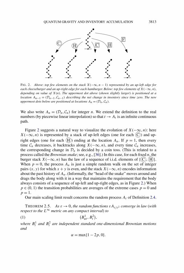
FIG. 2. Above: top few elements on the stack X(−∞, n − 1) represented by an up-left edge foreach cheeseburger and an up-right edge for each hamburger. Below: top few elements of X(−∞, n),depending on value of X(n). The uppermost dot above (shown slightly larger) is positioned at alocation An−1 = (Dn−1,Cn−1) describing the net change in inventory since time zero. The newuppermost dots below are positioned at locations An = (Dn,Cn).
We also write An = (Dn,Cn) for integer n. We extend the definition to the realnumbers (by piecewise linear interpolation) so that t → At is an infinite continuouspath.
Figure 2 suggests a natural way to visualize the evolution of X(−∞, n): hereX(−∞, n) is represented by a stack of up-left edges (one for each C ) and up-right edges (one for each H ) ending at the location An. If p = 1, then everytime Cn decreases, it backtracks along X(−∞, n), and every time Cn increases,the corresponding change in Dn is decided by a coin toss. (This is related to aprocess called the Brownian snake; see, e.g., [36].) In this case, for each fixed n, theburger stack X(−∞, n) has the law of a sequence of i.i.d. elements of { C , H }.When p = 0, the process An is just a simple random walk on the set of integerpairs (x, y) for which x + y is even, and the stack X(−∞, n) encodes informationabout the past history of An. (Informally, the “head of the snake” moves around anddrags the body along with it in a way that maintains the requirement that the bodyalways consists of a sequence of up-left and up-right edges, as in Figure 2.) Whenp ∈ (0,1) the transition probabilities are averages of the extreme cases p = 0 andp = 1.
Our main scaling limit result concerns the random process At of Definition 2.4.
THEOREM 2.5. As ε → 0, the random functions εAt/ε2 converge in law (withrespect to the L∞ metric on any compact interval) to(
B1αt ,B
2t
),(1)
where B1t and B2
t are independent standard one-dimensional Brownian motionsand
α = max{1 − 2p,0}.
3814 S. SHEFFIELD
In particular, the above theorem implies that Cn scales to ordinary Brownianmotion, which is not surprising since it is just a simple random walk on Z regard-less of p. When p = 0, the processes Dn and Cn are independent simple randomwalks on Z, and it is also unsurprising that An = (Dn,Cn) scales to an ordinarytwo-dimensional Brownian motion in this case. When p = 1 (and one only re-moves burgers from the top of the stack, because all orders are flexible), the lawof X(−∞, n) (for any fixed n) is that of an i.i.d. sequence of C and H values.In this case, the fact that inventory changes tend to be “well balanced” betweenhamburgers and cheeseburgers [so that the first term in (1) is identically zero andεAt/ε2 concentrates on the vertical axis as ε → 0] can be deduced from the law oflarge numbers. Indeed, when p = 1, the magnitude of Cn has order n1/2 with highprobability, while the magnitude of Dn has order n1/4 = o(n1/2). To see where then1/4 comes from, recall that C0 = 0 and condition on m := min{Cj : 0 ≤ j ≤ n}and on Cn, noting that C0 − m and Cn − m are both of order
√n. Note that the top
C0 −m burgers in the time zero stack fill the orders remaining in the reduced wordX(1, n), and the top Cn −m burgers in the time n stack are the types of the burgersin X(1, n). The types of the top C0 − m burgers in the time zero stack and the topCn − m burgers in the time n stack can then be determined with independent coin
tosses, so that Dn is of order√√
n = n1/4 = o(n1/2).The theorem states that as long as p ≥ 1/2 this balance continues to hold:
when n is large, the net inventory accumulation between time zero and n is closeto evenly divided between hamburgers and cheeseburgers, with high probability.When p < 1/2 the fluctuations of Dn are on the same order as those of Cn. Put dif-ferently, a LIFO retailer accumulates major inventory discrepancies (on the sameorder as the total inventory fluctuation) if and only if more than half of its cus-tomers have a product preference. Figure 3 illustrates sample trajectories of An forboth p < 1/2 and p > 1/2.
3. Inventory trajectories: Constructions and proofs. The primary goal ofthis section is to prove Theorem 2.5. On the way, we will establish some indepen-dently interesting lemmas involving properties of “excursion words” of varioustypes, equivalent formulations of the p = 1/2 phase transition, typical lengths ofrandom reduced words, and monotonicity properties for the time evolution of aninventory stack.
We recall that the optional stopping theorem states that if X0,X1,X2, . . . isa martingale (resp., supermartingale) and K is a bounded stopping time thenE[XK ] = E[X0] (resp., E[XK ] ≤ E[X0]). Furthermore, if K is an arbitrary (possi-bly unbounded) stopping time and X1,X2, . . . is a martingale (or supermartingale)whose values are bounded below then E[XK ] ≤ E[X0]. By symmetry, this alsoimplies that if K is an arbitrary stopping time and X1,X2, . . . is a martingale (orsubmartingale) whose values are bounded above then E[XK ] ≥ E[X0]. We willuse these facts frequently.
QUANTUM GRAVITY AND INVENTORY ACCUMULATION 3815
FIG. 3. Sample trajectory traced by An = (Dn,Cn) as n ranges from 0 to 100,000 when p = 0.25(left). Similar trajectories (axes not shown) when p = 0.75 (middle) and p = 1 (right). In each casewe use the same initial data: X(−∞,0) is an infinite stack alternating between burger types. Ineach case X(1), . . . ,X(100,000) are then chosen from μ and (Dn,Cn) updated accordingly forn ∈ {1,2, . . . ,100,000}. As n tends to infinity, and both axes are scaled by 1/
√n, the left trajec-
tory tends to a two dimensional Brownian motion with variance 1 − 2p = 0.5 times as large in theleft-right direction as the up-down direction. The middle and right trajectories tend to one-dimen-sional Brownian motions, concentrated on a vertical axis. (See Remark 3.17.)
3816 S. SHEFFIELD
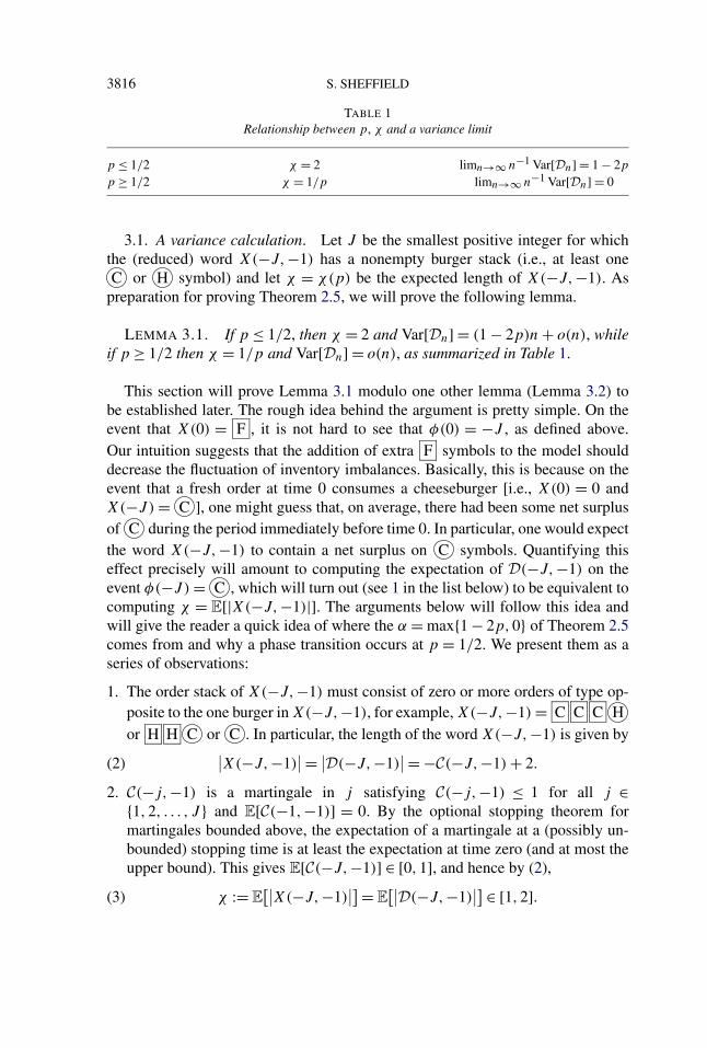
TABLE 1Relationship between p, χ and a variance limit
p ≤ 1/2 χ = 2 limn→∞ n−1 Var[Dn] = 1 − 2p
p ≥ 1/2 χ = 1/p limn→∞ n−1 Var[Dn] = 0
3.1. A variance calculation. Let J be the smallest positive integer for whichthe (reduced) word X(−J,−1) has a nonempty burger stack (i.e., at least oneC or H symbol) and let χ = χ(p) be the expected length of X(−J,−1). As
preparation for proving Theorem 2.5, we will prove the following lemma.
LEMMA 3.1. If p ≤ 1/2, then χ = 2 and Var[Dn] = (1 − 2p)n + o(n), whileif p ≥ 1/2 then χ = 1/p and Var[Dn] = o(n), as summarized in Table 1.
This section will prove Lemma 3.1 modulo one other lemma (Lemma 3.2) tobe established later. The rough idea behind the argument is pretty simple. On theevent that X(0) = F , it is not hard to see that φ(0) = −J , as defined above.Our intuition suggests that the addition of extra F symbols to the model shoulddecrease the fluctuation of inventory imbalances. Basically, this is because on theevent that a fresh order at time 0 consumes a cheeseburger [i.e., X(0) = 0 andX(−J ) = C ], one might guess that, on average, there had been some net surplusof C during the period immediately before time 0. In particular, one would expectthe word X(−J,−1) to contain a net surplus on C symbols. Quantifying thiseffect precisely will amount to computing the expectation of D(−J,−1) on theevent φ(−J ) = C , which will turn out (see 1 in the list below) to be equivalent tocomputing χ = E[|X(−J,−1)|]. The arguments below will follow this idea andwill give the reader a quick idea of where the α = max{1 − 2p,0} of Theorem 2.5comes from and why a phase transition occurs at p = 1/2. We present them as aseries of observations:
1. The order stack of X(−J,−1) must consist of zero or more orders of type op-posite to the one burger in X(−J,−1), for example, X(−J,−1) = C C C Hor H H C or C . In particular, the length of the word X(−J,−1) is given by∣∣X(−J,−1)
∣∣ = ∣∣D(−J,−1)∣∣ = −C(−J,−1) + 2.(2)
2. C(−j,−1) is a martingale in j satisfying C(−j,−1) ≤ 1 for all j ∈{1,2, . . . , J } and E[C(−1,−1)] = 0. By the optional stopping theorem formartingales bounded above, the expectation of a martingale at a (possibly un-bounded) stopping time is at least the expectation at time zero (and at most theupper bound). This gives E[C(−J,−1)] ∈ [0,1], and hence by (2),
χ := E[∣∣X(−J,−1)
∣∣] = E[∣∣D(−J,−1)
∣∣] ∈ [1,2].(3)
QUANTUM GRAVITY AND INVENTORY ACCUMULATION 3817
3. By (2) and (3), we have E[C(−J,−1)] = E[C(−1,−1)] = 0 if and only if χ =2. Since the optional stopping theorem implies
E[C(−1,−1)
] = E[C(−J,−1)1J≤n
] +E[C(−n,−1)1J>n
],
and the former term on the RHS tends to E[C(−J,−1)] we have
χ = 2 if and only if limn→∞E
[C(−n,−1)1J>n
] = 0.(4)
4. By (3), the expectation E[D(−J,−1)] exists and, by symmetry,
E[D(−J,−1)
] = 0.(5)
By (4) and the fact that |D(−n,−1)| ≤ |C(−n,−1)| = −C(−n,−1) if n < J ,
χ = 2 implies limn→∞E
[∣∣D(−n,−1)∣∣1J>n
] = 0.(6)
5. On the event X(0) = F the value D(0) is determined by X(0) independentlyof D(−J,−1). Hence, by (5), the expectation of D(0)D(−J,−1) restricted tothis event is zero. On the event X(0) = F we have J = φ(0) and hence D(0)
has sign opposite that of D(−J,−1). Since X(0) = F with probability p/2and [even after conditioning on X(0) = F ] we have E[|D(−J,−1)|] = χ , thisimplies
E[D(0)D(−J,−1)
] = −χp
2.(7)
6. On the event that J < n the expectation of D(0)D(−n,−J − 1) is zero, sinceD(−n,−J − 1) is independent of D(0) on this event [because X(−J,0) con-tains no F symbols, and one can swap the roles of hamburgers and cheeseburg-ers in the word X(−J )X(−J + 1) · · ·X(0) independently of the values of Xj
for j < −J ]. Thus the expectations of D(0)D(−n,−1) and D(0)D(−J,−1)
are the same on the event J < n (and trivially also the same on the event J = n).Thus,
E[D(0)D(−n,−1)
](8)
= E[D(0)D(−J,−1)1J≤n
] +E[D(0)D(−n,−1)1J>n
].
By (6), the latter term in (8) tends to zero as n → ∞ when χ = 2. Thus,
χ = 2 implies limn→∞E
[D(0)D(−n,−1)
] = −χp
2= −p.(9)
Using translation invariance of the law of Yj and (9), we obtain that
χ = 2 implies(10)
Var[Dn] =n∑
i=1
E[D(Yi)
2] + 2n∑
i=2
E[D(i)D(1, i − 1)
] = n − 2χp
2n + o(n),
which in particular implies that 1 − χp ≥ 0 so that
χ = 2 implies both p ≤ 1/2 and Var[Dn] = (1 − 2p)n + o(n).(11)
3818 S. SHEFFIELD
7. Lemma 3.2 below states that the conclusion of (6) holds even if χ = 2. Fornow, we note that that the above calculations show that the conclusions of (9)and hence (10) remain true when χ = 2 contingent on this claim:
limn→∞E
[∣∣D(−n,−1)∣∣1J>n
] = 0 implies Var[Dn] = n − χpn + o(n).(12)
From this and (3), we see the following:
Var[Dn] = o(n) and limn→∞E
[∣∣D(−n,−1)∣∣1J>n
] = 0 together imply(13)
1 − χp = 0 and hence χ = 1/p and p ≥ 1/2.
The following lemma will be proved later.
LEMMA 3.2. If χ = 2, then Var[Dn] = o(n) and limn→∞E[|D(−n,−1)| ×1J>n] = 0.
Lemma 3.2 states, in other words, that for each p ∈ [0,1], either the left state-ment in (11) (that χ = 2) is true or the left statements in (13) (that Var[Dn] = o(n)
and limn→∞E[|D(−n,−1)|1J>n] = 0) are true. We now claim that Lemma 3.1 isa consequence of (6), (11), (13), and Lemma 3.2. One hand Lemma 3.2 and (13)imply that if p < 1/2 then χ = 2 and (11) gives the top row of Lemma 3.1. Onthe other hand (11) implies that if p > 1/2 then χ = 2, and Lemma 3.2 and (13)give the bottom row. If p = 1/2, then the top and bottom row are equivalent, andwe must have χ = 2 [giving the desired result by (11)] since χ = 2 would lead toa contradiction using Lemma 3.1 and (13).
In preparation for proving Lemma 3.2, we will derive several additional conse-quences of the assumption that χ = 2 in Section 3.3.
3.2. Two simple finite expectation criteria. This section makes two simple ob-servations that will be useful in Section 3.3. The first is a special case of what issometimes called Wald’s identity. (We include a short proof for convenience incase the reader has not seen this before.)
LEMMA 3.3. Let Z1,Z2, . . . be i.i.d. random variables on some measurespace and ψ a measurable function on that space for which E[ψ(Z1)] is welldefined and finite. Let T be a stopping time of the process Z1,Z2, . . . with theproperty that E[T ] is finite. Then E[∑T
j=1 ψ(Zj )] is also well defined and finite.
PROOF. It is enough to consider the case that ψ is nonnegative (since we canwrite a general ψ as a difference of nonnegative functions). Since T is a stoppingtime, we know that for each fixed j , the value of Zj is independent of the event
QUANTUM GRAVITY AND INVENTORY ACCUMULATION 3819
that T ≥ j . Thus
E
[T∑
j=1
ψ(Zj)
]=
∞∑j=1
E[ψ(Zj )1T ≥j
](14)
=∞∑
j=1
E[ψ(Zj )
]E[1T ≥j ] = E
[ψ(Z1)
]E[T ].
�
LEMMA 3.4. Let Z1,Z2, . . . be i.i.d. random variables on some measurespace and let Zn be a nonnegative-integer-valued process adapted to the filtra-tion of the Zn (i.e., each Zn is a function of Z1,Z2, . . . ,Zn) that has the followingproperties:
1. Bounded initial expectation: E[Z1] < ∞.2. Positive chance to hit zero when close to zero: For each k > 0, there exists a
positive pk such that P[Zn+1 = 0|Z1, . . . ,Zk] ≥ pk on {Zn = k}.3. Uniformly negative drift when far from zero: There exist positive constants C
and c such that E[Zn+1 −Zn|Z1, . . . ,Zk] ≤ −c on {Zn ≥ C}.4. Bounded expectation when near zero: There further exists a constant b such
that E[Zn+1|Z1, . . . ,Zn] < b on {Zn < C}.Then
E[min{n : Zn = 0}] < ∞.
PROOF. The uniformly negative drift assumption implies that the quantityYn = Zn + cn is a supermartingale until time K = min{n ≥ 0 : Zn < C}. Inparticular, this fact together with the optional stopping theorem implies that asa function of k the quantity E[YK∧k] is bounded above independently of k. Onthe event K ≥ k we have Yk ≥ ck. Since YK∧k is non-negative, this implies thatckP[K ≥ k] ≤ E[YK∧k]. In particular, this implies that limk→∞P[K ≥ k] = 0 sothat K is a.s. finite.
Next, by the optional stopping theorem for non-negative supermartingales,E[YK ] ≤ E[Y1] which implies E[cK] ≤ E[Y1] and E[K] ≤ E[Y1]/c. Now letT1, T2, . . . denote the successive times when Zn < C. Then we claim that a similaranalysis implies that E[Tk+1 − Tk|Z1,Z2, . . . ,ZTk
] ≤ β for some positive con-stant β . To carry out this analysis, we will write Yn = ZTk+n + cn, and note thatthe same argument as above (using probability conditioned on Z1,Z2, . . . ,ZTk
andnoting that E[Y1|Z1,Z2, . . . ,ZTk
] ≤ b + c) shows that
E[Tk+1 − Tk|Z1,Z2, . . . ,ZTk] ≤ E[Y1|Z1,Z2, . . . ,ZTk
]/c ≤ (C + c)/c =: β.
Next, recall that whenever Zn < C, there is a probability of at least δ = min{pk :k ≤ C} > 0 that Zn+1 = 0. This implies that if S := min{n : Zn = 0} then P[S >

3820 S. SHEFFIELD
Tk] ≤ δk−1. Since
E[S] ≤ E[T1] + E
[ ∞∑k=1
(Tk+1 − Tk)1S>Tk
](15)
≤ E[K] +∞∑
k=1
P[Tk > S]E[Tk+1 − Tk|S > Tk](16)
≤ E[K] +∞∑
k=1
δk−1β < ∞.(17)�
3.3. Excursion words. In Section 3.1, we considered the random wordX(−J,−1), where J was the smallest integer for which this word had at leastone C or H symbol. We found that the expected word length E[|X(−J,−1)|]was a constant χ ∈ [1,2]. In this section, we will consider different words andshow that they all have finite expected length provided that χ < 2.
Suppose that K is the smallest k ≥ 0 for which Ck+1 = C(1, k + 1) < 0. IfX(1) ∈ { C , H , F } then K = 0. Otherwise, K is a positive value for which CK =C(1,K) = 0, so that X(1,K) is “balanced” in the sense that it has the same numberof burgers as orders. Call E = X(1,K) the excursion word beginning at time zero(writing E =∅ if K = 0). We make a few observations about E:
1. E a.s. contains no F symbols. [Indeed, one can check inductively that X(1, k)
contains no F symbols for any 1 ≤ k ≤ K .]2. If p = 1, then E = ∅ almost surely.3. The law of K is independent of p ∈ [0,1]. Its law is that of the number of steps
taken by a simple random walk on Z, started at 0, before it first hits −1. (Inparticular, E[K] = ∞.)
We denote by Vi the symbol corresponding to the ith record minimum of Cn,counting forward from zero, if i is positive, and the −ith record minimum of Cn,counting backward from zero, if i is negative (see Figure 4). We will introducenotation to describe the locations of the Vi in the proof of Lemma 3.5.
Denote by Ei the reduced form of the word strictly in between the symbols cor-responding to Vi and Vi−1 (if i is positive) or between Vi and Vi+1 (if i is negative),where V0 is for the moment formally taken to be the “zero point” located betweenthe symbols X(0) and X(1) (see Figure 4). We do not define Ei for i = 0. Notethat the Vi are i.i.d. equal to H or C (each with probability 0.5) when i < 0 andequal to H , C , or F [with probabilities (1−p)/2, (1−p)/2 and p] when i > 0.The Ei are i.i.d. excursion words, each with same law as the E described above,and are independent of the Vi . (The fact that E1 and E−1 are identically distributedfollows from the fact that an excursion of the simple random walk Cn is equivalentin law to its time reversal. Indeed, once we condition on the trajectory of Cn over
QUANTUM GRAVITY AND INVENTORY ACCUMULATION 3821
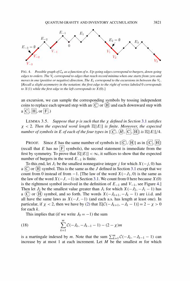
FIG. 4. Possible graph of Cn as a function of n. Up-going edges correspond to burgers, down-goingedges to orders. The Vi correspond to edges that reach record minima when one starts from zero andmoves in one (positive or negative) direction. The Ei correspond to the excursions in between the Vi .[Recall a slight asymmetry in the notation: the first edge to the right of vertex labeled 0 correspondsto X(1) while the first edge to the left corresponds to X(0).]
an excursion, we can sample the corresponding symbols by tossing independentcoins to replace each upward step with an C or H and each downward step witha C , H , or F .)
LEMMA 3.5. Suppose that p is such that the χ defined in Section 3.1 satisfiesχ < 2. Then the expected word length E[|E|] is finite. Moreover, the expectednumber of symbols in E of each of the four types in { C , H , C , H } is E[|E|]/4.
PROOF. Since E has the same number of symbols in { C , H } as in { C , H }(recall that E has no F symbols), the second statement is immediate from thefirst by symmetry. To prove that E[|E|] < ∞, it suffices to show that the expectednumber of burgers in the word E−1 is finite.
To this end, let J1 be the smallest nonnegative integer j for which X(−j,0) hasa C or H symbol. This is the same as the J defined in Section 3.1 except that wecount from 0 instead of from −1. [The law of the word X(−J1,0) is the same asthe law of the word X(−J,−1) in Section 3.1. We count from 0 here because X(0)
is the rightmost symbol involved in the definition of E−1 and V−1, see Figure 4.]Then let J2 be the smallest value greater than J1 for which X(−J2,−J1 − 1) hasa C or H symbol, and so forth. The words X(−Jk+1,−Jk − 1) are i.i.d. andall have the same laws as X(−J,−1) (and each a.s. has length at least one). Inparticular, if χ < 2, then we have by (2) that E[C(−Jk+1,−Jk − 1)] = 2 − χ > 0for each k.
This implies that (if we write J0 = −1) the summ∑
k=1
C(−Jk,−Jk−1 − 1) − (2 − χ)m(18)
is a martingale indexed by m. Note that the sum∑m
k=1 C(−Jk,−Jk−1 − 1) canincrease by at most 1 at each increment. Let M be the smallest m for which

3822 S. SHEFFIELD
∑mk=1 C(−Jk,−Jk−1 −1) = 1. The fact that
∑mk=1 C(−Jk,−Jk−1 −1) = 1 is a sum
of i.i.d. integer-valued random variables, each with expectation greater than zero,together with the law of large numbers implies that the sum tends to ∞ as m → ∞.Since each of the random variables in the sum is at most 1 we conclude thatM < ∞ a.s. Since the martingale (18) is bounded above up to time M , the optionalstopping theorem for martingales bounded above implies that the expected valueof (18) at this stopping time is at least 0, which implies that E[1 − (2 − χ)M] ≥ 0and hence E[M] ≤ 1/(2 − χ). Since C(−JM,0) = 1, it follows that −JM is leftof the location of V−1 (since the latter corresponds to the first time the countreaches 1, counting left from zero). Since the number of burgers in X(−j,0) isincreasing in j , it follows that X(−JM,0) has at least as many burgers as V−1E−1.The expectation of the number of burgers in X(−JM,0) is finite [since X(−JM,0)
has at most M burgers], and hence so is the expectation of the latter. �
The lemmas that follow will involve several sequences related to the Jm definedabove (each defined for m ≥ 1). For convenience, we define them here:
1. mth empty order stack: Om is the mth smallest value of j ≥ 0 with the propertythat X(−j,0) has an empty order stack. We have not proved that O1 is a.s.finite, but if it is then we may observe that the words X(−Om,−Om−1 − 1) arei.i.d. (if we formally set O0 = −1) and that each has an empty order stack.
2. mth empty burger stack: Bm is the mth smallest value of j ≥ 1 with the propertythat X(1, j) has an empty burger stack. We have not proved that B1 is a.s. finite,but if it is, then we may observe that the words X(Bm−1 + 1,Bm) are i.i.d. (ifwe formally set B0 = 0) and that each has an empty burger stack.
3. mth left record minimum: Lm is the smallest value of j ≥ 0 for whichC(−j,0) = m. Thus X(−Lm,0) = V−mE−m · · ·V−1E−1 and X(−Lm,
−Lm−1 − 1) = V−mE−m (if we formally set L0 = −1).4. mth right record minimum: Rm is the smallest value of j ≥ 1 for which
C(1, j) = −m. Thus X(1,Rm) = E1V1 · · ·EmVm and X(Rm−1 + 1,Rm) =EmVm (if we formally set R0 = −1).
5. mth hamburger-order-free left minimum: LHm is the mth smallest value of j ≥ 0
with the property that X(−LHj ,0) has no hamburger orders and LH
j = Lj ′ for
some j ′ [i.e., −LHj corresponds to a new record minimum of C(·,0)]. As in
the cases above, the words X(−LHj ,−LH
j−1 − 1) are i.i.d., and each one is aproduct of some sequence of words of the form X(−Lj ′,−Lj ′−1 − 1).
6. mth hamburger-free right minimum: similarly, RHm is the mth smallest value of
j ≥ 1 with the property that X(1,RHm ) has no hamburgers and RH
j = Rj ′ forsome j ′.
LEMMA 3.6. The following are equivalent:
1. E[|E|] < ∞.
QUANTUM GRAVITY AND INVENTORY ACCUMULATION 3823
2. E[|X(−LH1 ,0)|] < ∞.
3. E[|X(1,RH1 )|] < ∞.
4. O1 is a.s. finite and E[|X(−O1,0)|] < ∞.5. B1 is a.s. finite and E[|X(1,B1)|] < ∞.
PROOF. 1 implies 2: Assume 1. Recall that the words E−j are i.i.d., thateach a.s. has no F symbols and as many orders as burgers (possible example:
C H H C C C C H ), that the expected number of symbols of each of the
types { C , H , C , H } in E−1 is finite, and that these expectations are equal. Re-call also that the Vj (for j < 0) are independent i.i.d. samples from { C , H }. LetH(m) be the number of hamburger orders in X(−Lm,0) = V−mE−m · · ·V−1E−1.Note that for any m > 1 we have that
H(m) = max{H(m − 1) − hm,0
} + om,(19)
where hm is the number of hamburgers in V−mE−m and om is the number of ham-burger orders in V−mE−m. Note that the pair (hm, om) is independent of H(m−1).Note also that E[hm] = E[om] + 0.5 (since the expected number of hamburger or-ders in E equals the expected number of hamburgers and V−m = H with proba-bility 0.5).
Now we can rewrite (19), using the fact that max{A,0} = A − 1A<0A, as
H(m) − H(m − 1) = om − hm + (hm − H(m − 1)
)1{H(m−1)−hm<0},
and E[(hm − k)1hm>k] ≤ E[hm1hm>k] ↓ 0 as k → ∞ by assumption. Thus, thereexists a C > 0 such that for all k > C we have E[H(m) − H(m − 1)|H(m − 1) =k] ≤ −0.4. It follows from Lemma 3.4, applied with Zm = H(m) and Zm =V−mE−m, that the expected number of V−jE−j sequences concatenated to pro-duce X(−LH
1 ,0) is finite, and it then follows from 1 and Lemma 3.3 that theexpected sum of the lengths of these words is finite.
1 implies 3: The argument used to show that 1 implies 2 applies almost verbatimhere, using Rm in place of Lm.
2 implies 4: We use the argument used to show 1 implies 2. In that case,we concatenated i.i.d. words of the form X(−Lm,−Lm−1 − 1) = V−mE−m
until we produced a word with no hamburger orders, which was equal toX(−LH
1 ,0). In this case, we start by concatenating the i.i.d. words of the formX(−LH
m,−LHm−1 − 1), each of which has no orders of type H or F (possible
example: C C C C C H C C C H ), and we continue until we produce aword with no orders at all. This word is necessarily at least as long as X(−O1,0)
[since the burger stack is increasing in time, and X(−O1,0) corresponds to thefirst time the order stack is empty], so it suffices to bound its expected length.
We are assuming that the expected length of X(−LH1 ,0) is finite; since this
word has at least as many burgers as X(−L1,0), this implies that the expected
3824 S. SHEFFIELD
number of burgers in X(−L1,0) is also finite, and since the number of orders inX(−L1,0) is one less than the number of burgers, we find that the expected totallength of X(−L1,0) is finite, as is the expected total length of E−1. That is, wehave established that 2 implies 1. We may therefore use the fact (established at theend of the 1 implies 2 argument) that the expected number of V−jE−j sequencesconcatenated to produce X(−LH
1 ,0) is some finite number k.Note that the expected net number of cheeseburgers in X(−Lm,−Lm−1 − 1) =
V−mE−m (i.e., the expected number of C symbols minus the number of C sym-bols) is 1/2, since this net number is additive when we concatenate words withno F symbols. We similarly conclude by (14) that the expected net number ofcheeseburgers in X(−LH
1 ,0) is k/2, where k is as defined just above.As we concatenate i.i.d. copies of the word X(−LH
1 ,0), the number of C sym-bols in the reduced form of the concatenated word is a Markov chain on Z+. Theabove observations imply that the expected change in this Markov chain value,during a step that starts at position j , is a value that tends to −k/2 as j → ∞.For any j , this expected change is bounded above by the finite expected length ofX(−LH
1 ,0). Thus, Lemma 3.4, implies that the expected number of steps until thischain reaches zero is finite. Similarly, Lemma 3.3 then implies that the expectedtotal length of the words concatenated is finite.
3 implies 5: This is essentially the same as the proof that 2 implies 4.Either 4 or 5 implies 1: Note that the number of burgers in X(−O1,0) is at least
the number in E−1, and the number of orders in X(1,B1) is at least the numberin E1. Thus if either E[|X(−O1,0)|] < ∞ or E[|X(1,B1)|] < ∞, then (recallingthat the expected number of orders in E equals the expected number of burgers inE) we have E[|E|] < ∞. �
LEMMA 3.7. If E[|E|] < ∞, then the limit, as n → ∞, of the fractions ofH symbols among the top n elements in X(−∞,0) is equal to 0.5 almost surely.
Similarly, as n tends to infinity, the fraction of C , H and F symbols among theleftmost n elements of X(1,∞) tend almost surely to constants (the first two equal,by symmetry). These constants are all positive (except in case p = 1, where onehas only F symbols and no C or H symbols).
On the other hand, if E[|E|] = ∞ then the limit as n → ∞ of the fraction of Fsymbols among the leftmost n elements of X(1,∞) tends almost surely to zero.
PROOF. Consider the sequence of words X(−k,0), indexed by positive k. Aswe have noted before, the words X(−Om,−Om−1 − 1) are i.i.d., each consistingentirely of burgers, and X(−∞,0) is the concatenation of these all-burger words.Lemma 3.6 implies that if E[|E|] < ∞, then the lengths of these burger sequenceshave finite expectation, and the law of large numbers then implies the number ofhamburgers and cheeseburgers in X(−Om,0) are both [up to o(m) errors] givenby constant multiples of m, almost surely. This implies the first statement in the
QUANTUM GRAVITY AND INVENTORY ACCUMULATION 3825
lemma. The proof of the second statement is analogous, using Bm instead of Om.To see that the constants are positive, it suffices to observe that X(1,B1) has somepositive probability of containing an order of each of the three order types.
For the final statement, we note that an F symbol can be added to the orderstack of the sequence X(1, k) only at times when the burger stack is empty. Thenumber of F symbols in X(1,Bm) can grow as a function of m, but it can growby at most 1 each time that m increases by 1. If E[|E|] = ∞, then Lemma 3.6 andthe law of large numbers imply that the number of orders in X(1,Bm) a.s. growsfaster than any constant times m, while the number of F symbols grows like aconstant times m. �
The following proposition is not needed for the proof of Theorem 2.5, but weinclude it because it will be interesting from the point of view of random planarmaps. (In a sense, it will imply that the infinite random surface models one obtainswhen p > 1/2 a.s. have infinitely many small bottlenecks surrounding any givenpoint.)
PROPOSITION 3.8. Let K be the infimum over the set of positive numbers suchthat there exist m− < 0 and m+ > 0 such that:
1. X(m−,0) is a word with no orders and K burgers.2. X(1,m+) is a word with no burgers and K orders.3. X(m−,m+) = ∅.
If E[|E|] < ∞, then K is a.s. finite and E[K] < ∞.
PROOF. Assume E[|E|] < ∞. As noted in the proof of Lemma 3.7, the gapsbetween am := |X(−Om,0)| (as m increases) and between bm := |X(1,Bm)| (asm increases) are i.i.d. positive random variables with finite expectation (and clearlyevery possible positive gap length has positive probability).
Write αk = k − max{am : am ≤ k} and βk = k − max{bm : bm ≤ k}. Both αk andβk can be understood as ergodic Markov chains. To see this, note that if αk = j ,then αk+1 ∈ {j + 1,0} and P[αk+1 = 0|αk = j ] = P[a1 = j + 1|a1 > j ]. The tran-sition kernel for βk can be written similarly. Since a· and b· each have incrementswith finite expectation, the corresponding ergodic Markov chains assume the value0 (at stationarity) with probability one over the corresponding expectation. Sinceα· and β· are independent, the pair (α·, β·) is also a Markov chain that (at station-arity) assumes the value (0,0) with positive probability.
Call a nonnegative integer M a “match up length” if there exists an i such thatai = |X(−Oi,0)| = M and a j such that bj = |X(1,Bj )| = M . The match uplengths are a random subset of Z+ and correspond to the k for which (αk, βk) =(0,0). The discussion above implies that the gaps between successive match uplengths are i.i.d. random variables with finite expectation. Denote by Mk the kthsuch match up length.
3826 S. SHEFFIELD
For each Mk , we have a word X(−Oi,0) of length Mk comprised entirely ofburgers and a word X(1,Bj ) of length Mk , comprised entirely of orders. We claimthat X(−Oi,Bj ) is a word that consists of a sequence of orders of one type (eitherC or H ) followed by a same-length sequence of burgers of opposite type (eitherC or H ), for example,
C C C C C H H H H H .
[This can be seen by starting with the all-burger word X(−Oi,0) and multiplyingon the right by the symbols in X(1,Bj ) one at a time. The only way there can beorders in X(−Oi,Bj ) is if all of the burgers of one type are consumed before thisprocess terminates, and in that case only orders corresponding to that burger typecan appear in X(−Oi,Bj ).] When we shift from k to k + 1, we multiply this wordon the left and right by random words W1 and W2. We know that C(W1)+C(W2) =0. By symmetry, the expected number of symbols of type H in this pair of wordsequals the expected number of symbols of type C . (These expectations are finiteby Lemma 3.6.) Similarly for H and C symbols. The expected number of Fsymbols is some positive constant a.
If the length of X(−Oi,Bj ) is long enough, then the probability that either W1or W2 is longer than half of that length is close to zero. Thus, conditioned on thelength being at least some constant value, the expected change in length as onegoes from k to k + 1 is close to −a/2. It then follows from Lemma 3.4 that theexpected value of the smallest k for which this length is zero is finite, and the resultthen follows from Lemma 3.3. �
3.4. Some monotonicity observations. In this section, it will be convenient tofix a semi-infinite stack present at time zero [the stack X(−∞,0)] and also to relaxthe assumption in Definition 2.4 that (Dn,Cn) = (0,0). To give some notation forthis, let S0 be a semi-infinite stack of burgers containing infinitely many burgersof each type together with a corresponding diagram in R
2 such as the one given inFigure 2. The diagram is determined by the burger stack once we know the locationof the uppermost vertex (the tip) in Figure 2, which we now allow to be any latticepoint of Z2 whose coordinate sum is even. Slightly abusing notation, we will write(D0,C0) for the location of the tip of S0 (which, in this section only, we do notrequire to be at the origin).
Given S0, we can generate a sequence of stacks S1, S2, . . . in the usual mannerby applying the moves in Figure 2 that correspond to X(1),X(2), . . . . For n > 0,we write (Dn,Cn) := (D0 + D(1, n),C0 + C(1, n)) as before, so that (Dn,Cn) isthe location of the tip of Sn.
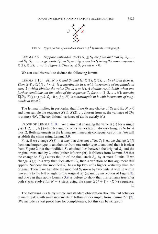
Given any such embedded stacks S and S, we write S ≤ S if the tips of the pathlie on the same horizontal line and the path describing S (as in Figure 2) lies to theleft of the path describing S—that is, every horizontal line intersects the S path ata point equal to or left of where it intersects the S path, see Figure 5. The followinglemma is immediate from an inspection of the cases in Figure 2.
QUANTUM GRAVITY AND INVENTORY ACCUMULATION 3827
FIG. 5. Upper portion of embedded stacks S ≤ S (partially overlapping).
LEMMA 3.9. Suppose embedded stacks S0 ≤ S0 are fixed and that S1, S2, . . .
and S1, S2, . . . are generated from S0 and S0 respectively using the same sequenceX(1),X(2), . . . as in Figure 2. Then Sn ≤ Sn for all n > 0.
We can use this result to deduce the following lemma.
LEMMA 3.10. Fix N > 0 and S0 and let X(1),X(2), . . . be chosen from μ.Then E[DN |X(j) : j ≤ k] is a martingale in k with increments of magnitude atmost 2 (which obtains the value DN at k = N ). A similar result holds when onefurther conditions on the value of the sequence Cn for n ∈ {1,2, . . . ,N}: namely,E[DN |X(j) : j ≤ k,Cj : 0 ≤ j ≤ N ] is a martingale in k with increments of mag-nitude at most 2.
The lemma implies, in particular, that if we fix any choice of S0 and fix N > 0and then sample the sequence X(1),X(2), . . . chosen from μ, the variance of DN
is at most 4N . (The conditional variance of CN is exactly N .)
PROOF OF LEMMA 3.10. We claim that changing the value X(j) for a singlej ∈ {1,2, . . . ,N} (while leaving the other values fixed) always changes DN by atmost 2. Both statements in the lemma are immediate consequences of this. We willestablish the claim using Lemma 3.9.
First, if we change X(j) in a way that does not affect Cj [i.e., we change X(j)
from one burger type to another, or from one order type to another] then it is clearfrom Figure 2 that the modified Sj obtained lies between the original Sj and theoriginal translated by 2 units (either left or right). It follows from Lemma 3.9 thatthe change to X(j) alters the tip of the final stack SN by at most 2 units. If wechange X(j) in a way that does affect Cj , then a variation of this argument stillapplies. Suppose the modified Sj has a tip two units higher vertically than theoriginal. Then if we translate the modified Sj down by two units, it will lie withintwo units to the left or right of the original Sj (again, by inspection of Figure 2),and one can then apply Lemma 3.9 as before to show that this remains true afterboth stacks evolve for N − j steps using the same X(j + 1) · · ·X(n) sequence.
�
The following is a fairly simple and standard observation about the tail behaviorof martingales with small increments. It follows for example, from Lemma 2 of [2].(We include a short proof here for completeness, but this can be skipped.)
3828 S. SHEFFIELD
LEMMA 3.11. Let βj be a martingale in j whose increments have magnitudeat most 1, with β0 = 0. Then for each real a > 0 and integer n > 0 we have
P(
maxj∈{1,2,...,n}n
−1/2βj ≥ a)
≤ e−a+1/2.
PROOF. First, we observe that eb+e−b
2 ≤ eb2/2 for all b. [Indeed, by Taylorexpansion, the left side is 1 + b2/2! + b4/4! + b6/6! + · · · while the right sideis 1 + b2/(211!) + b4/(222!) + b6/(233!) + · · · .] Thus, if the increments of βj
were exactly ±1 (each with probability 1/2), with β0 = 1, then we would haveE[ebβ1] ≤ eb2/2 and E[ebβ1−b2/2] ≤ 1. We claim that the same is true if we al-low for β1 /∈ {−1,1} and insist only that |β1| ≤ 1 a.s. and Eβ1 = 0. (Indeed, onemay first choose an increment β1, and then, given this, choose a “modified incre-ment” β ′
1 ∈ {−1,1} using a biased coin whose probability is chosen so that con-ditional expectation of the modified increment is β1. Jensen’s inequality impliesE[ebβ1] ≤ E[ebβ ′
1].) The argument above shows more generally that ebβj−jb2/2 is asupermartingale indexed by j .
Taking b = n−1/2 produces a supermartingale in j whose value at time j = 0 is1 and whose value at general j time is en−1/2βj−j/(2n). The expectation of the latterquantity is at most 1, by the optional stopping theorem, so the probability that itever reaches ea−1/2 is at most e−a+1/2. To conclude, we note that n−1/2βj ≥ a
implies en−1/2βj−j/(2n) ≥ ea−1/2 for j ∈ {1,2, . . . , n}. �
LEMMA 3.12. Fix any p ∈ [0,1]. Fix the time zero stack S0. Then there arepositive constants C1 and C2 such that, for any choice of S0, a > 0, and n ≥ 1, theprobability that |Dj | > a
√n for some j ∈ {0,1,2, . . . , n} is at most C1e
−C2a .
PROOF. Without loss of generality, assume C0 = D0 = 0. To sample X(1),X(2), . . . we may first sample the sequence C1,C2, . . . and then conditioned onthat choose the types of the burgers and orders (which in turn determine the Dj
sequence). Write M = a√
n/8 and note that
P
{max
j∈{1,2,...,n} |Cj | > M}
≤ 2e−a/8+1/2(20)
by Lemma 3.11. Thus, we may restrict attention to the event En that this does notoccur, in which case we are conditioning on values of Cj that satisfy |Cj | ≤ M forj ∈ {1,2, . . . , n}.
Using Lemma 3.10, we have that
mj := E[Dn|X(i) : i ≤ j,Ci : 0 ≤ i ≤ n
](21)
is a martingale in j for j ∈ {0,1, . . . , n} with increments of size at most 2. Thevalue of Dj depends on the stack at time j and does not depend on any of the
QUANTUM GRAVITY AND INVENTORY ACCUMULATION 3829
edges in S0 that lie below −M . This is because if one considers two differentchoices of S0 which agree above level −M , and then takes the same choice ofsymbols X(0),X(1),X(2), . . . whose values imply |Cj | ≤ M for j ∈ {1,2, . . . , n},then by induction the updated stack Sj will look the same above level −M for eachj between 0 and n, and since all F symbols get matched to burgers above level−M , we may conclude that (on the event En) Dj does not depend on the choice ofS0 below level −M . We can also rewrite (21) as mj = E[Dn|Sj ,Ci : 0 ≤ i ≤ n].
Now fix some value j ∈ {1,2, . . . , n} and let Sj be the stack obtained by swap-ping the burgers in Sj above level −M and subsequently translating the stackby 4M units to the left (i.e., translating the stack by the amount that ensuresthat the corresponding Dj value is translated by 4M , but Cj remains the same).Then we see that Sj lies strictly to the left of Sj . One can then see inductively(by Lemma 3.9) that this will continue to be the case if we evolve both stacksin parallel by adding the same symbols Xj+1,Xj+2, . . . to each. Let Dj be thediscrepancy of Sj , so that (by definition) we have Dj = Dj − 4M . Let Di forj ≤ i ≤ n be obtained by letting the stack evolve by the addition of the sym-bols Xj + 1,Xj + 2, . . . ,Xn. Set mj = E[Dn|Sj ;Ci ,0 ≤ i ≤ n], which is alsoE[Dn|Sj ,Ci : 0 ≤ i ≤ n]. Now observe by symmetry that on the event En we have
Dj − mj = −(Dj − mj).(22)
By the fact (noted above) that Si is left of Si for j ≤ i ≤ n one has Dn ≤ Dn andtherefore mj ≤ mj , and we also recall that Dj = Dj − 4M . Rewriting the LHSof (22) using these two facts, we get
Dj − 4M − mj ≤ −Dj + mj,
which implies Dj − mj ≤ 2M on En.An analogous statement holds if we define Sj using translation to the right in-
stead of to the left. Thus, on the event En, we have |Dj − mj | ≤ 2M = a4
√n
for all j ∈ {0,1, . . . , n}. Thus, in order to have |Dj − D0| ≥ a√
n for somej ∈ {1,2, . . . , n} we must have |mj − m0| ≥ a
√n/2. Applying Lemma 3.11 to
mj/2, we find that the conditional probability (given En) that |mj − m0| exceeds√na/2 on the interval {1,2, . . . , n} is at most e−a/4+1/2. This combined with (20)
gives the lemma. �
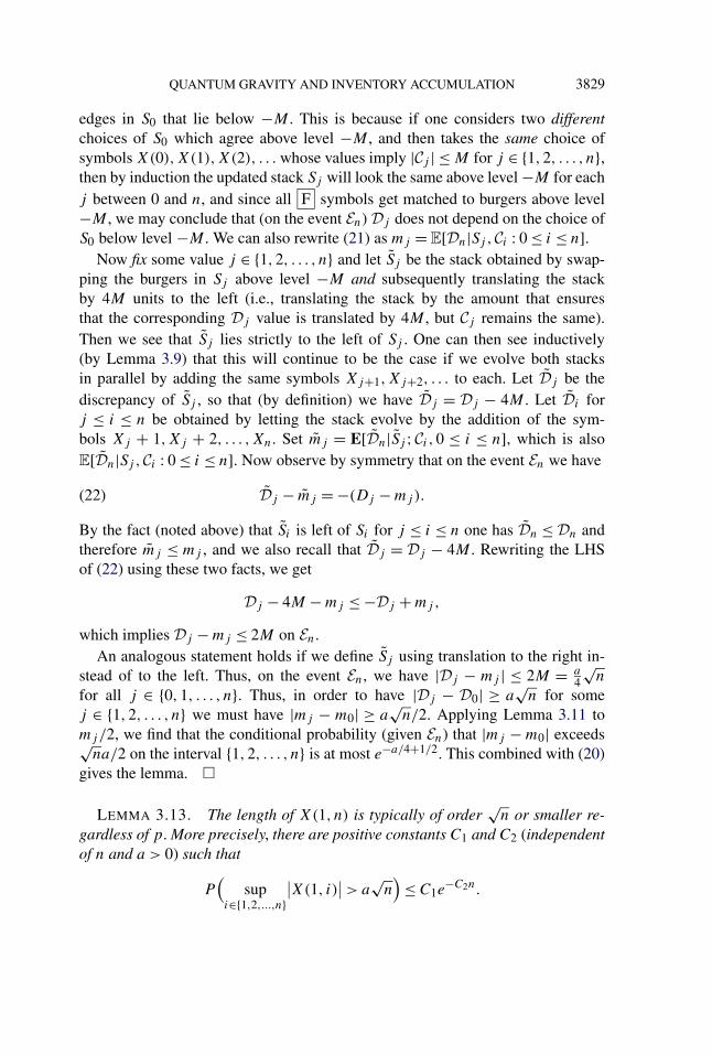
LEMMA 3.13. The length of X(1, n) is typically of order√
n or smaller re-gardless of p. More precisely, there are positive constants C1 and C2 (independentof n and a > 0) such that
P(
supi∈{1,2,...,n}
∣∣X(1, i)∣∣ > a
√n)
≤ C1e−C2n.

3830 S. SHEFFIELD
PROOF. Fix an initial stack S0 to be alternating between C and H . Thenobserve that if Dk and Ck both fluctuate by at most a
√n/5, as k ranges from 1
to n, then no burger on the stack S0 strictly below height −2a√
n/5 will havebeen consumed during the first n steps. (If the first burger below that height to beconsumed were consumed at step j , then all of the burgers above it in the stack atstep j—let k be the number of such burgers—would have to be of the same type.This would require that either k < a
√n/5, in which case |Cj | would have to exceed
the assumed bound, or that k ≥ a√
n/5, in which case |Dj | would have to exceedthe assumed bound, since all the burgers below the top k must strictly alternatebetween C and H .) Thus, on this event the total number of orders in X(1, i) isless than 2a
√n/5 for each i ∈ {1,2, . . . , n}. Since Ck fluctuates by at most a
√n/5
this also implies that the total number of burgers in X(1, i) is at most 3a√
n/5 foreach i ∈ {1,2, . . . , n}, and hence |X(1, i)| < a
√n for each i ∈ {1,2, . . . , n}. The
result thus follows from Lemma 3.12 and the analogous bound that applies whenD is replaced by C. �
3.5. Proof of Lemma 3.2. Lemma 3.2 should not seem very surprising in lightof the results we have established so far. Lemma 3.5 and Lemma 3.7 show thatwhen the Lemma 3.2 hypothesis holds (i.e., χ = 2) the stack X(−∞,0), embed-ded in the manner of Figure 2, scales to a vertical line a.s. as one zooms out. Itis thus natural to expect that the left-right fluctuation of the time-evolution of thestack is small compared to the up-down fluctuation. We divide Lemma 3.2 intoLemmas 3.14 and 3.16, which we state and prove below.
LEMMA 3.14. If χ = 2, then Var[D(n)] = o(n).
PROOF. First, we claim that if χ = 2 then n−1/2Dn tends to zero in probability.To see this, recall that the stacks X(−∞,0) and X(−∞, n) agree in law, and thatthe collection of the top a
√n burgers (for any fixed a) is likely to contain a roughly
even distribution of hamburgers and cheeseburgers, in the sense of Lemma 3.7. ByLemma 3.13, the probability that the two stacks agree except for the top a
√n
burgers [i.e., that one can find j, k ≤ a√
n such that X(−∞,0) with the top j
burgers removed is the same as X(−∞, n) with the top k burgers removed] is aquantity that remains bounded below as n tends to infinity, and the bound can bemade arbitrarily close to 1 by making a large enough. It follows from this that therandom variables n−1/2Dn tend to zero in probability. We still need to show thatthe variances E[n−1D2
n] tend to zero. This follows from the fact that the randomvariables n−1D2
n tend to zero in probability, together with the uniform bounds ontheir tails given by Lemma 3.12. �
LEMMA 3.15. If Var[D(n)] = o(n) then n−1/2 max{|Dj | : 1 ≤ j < nt} con-verges to zero in probability for each fixed t > 0.
QUANTUM GRAVITY AND INVENTORY ACCUMULATION 3831
PROOF. The variance assumption immediately implies that n−1/2D nt� con-verges to zero in probability for each fixed t . It also implies that the joint law ofn−1/2D nt� at any fixed collection of t values tends to zero in probability.
Now, suppose that we divide the first t units of time into equal increments oflength δ (for some small δ). Then on each such increment, we would guess thatwith high probability the fluctuation of n−1/2D tn�, as t ranges through an intervalof length δ, should be very small when n is sufficiently large and δ is small andfixed. Indeed, the bound in Lemma 3.12 (applied with a = δ1/6) implies that theprobability that there is even a single interval on which the fluctuation magnitude isgreater than aδ1/2 = δ2/3 will remain bounded above by some constant as n → ∞,and this constant can be made arbitrarily small by taking δ sufficiently small. Sincewe can take δ as close to zero as we like, the lemma follows. �
LEMMA 3.16. If χ = 2 and Var[D(n)] = o(n), then
limn→∞E
[∣∣D(−n,−1)∣∣1J>n
] = 0.
PROOF. Let us assume Var[D(n)] = o(n) and proceed to derive the conclu-sion of the lemma. Let I be the smallest value of j ≥ 0 for which C(−j,−1) = 1.For each n, let μn be the measure whose Radon–Nikodym derivative with re-spect to μ is given by the (a.s. nonnegative) quantity (1 − C(−n,−1))1I≥n. Since(1 − C(−n,−1)) is a martingale (which reaches zero at time I ) the optional stop-ping theorem implies that the expectation of (1 − C(−n,−1))1I≥n is 1, so that μn
is in fact a probability measure. Informally, μn is the measure obtained from μ byconditioning on aj := (1 − C(−j,−1)) being positive until time n and multiply-ing the probability of each X(−n) · · ·X(−1) sequence by a quantity proportionalto an.
Note that if we just consider the law μ conditioned on having aj eventually hitsome C > n before hitting zero, then the law of {a1, a2, . . . , an} under this condi-tional law agrees with μn. In both measures, if we are given the values of ai upto some j ∈ {0,1, . . . , n − 1}, then the conditional probabilities that aj goes up toaj + 1 and down to aj − 1 are proportional, respectively, to aj + 1 and aj − 1.Thus, there exists a measure μ∞ whose law restricted to X(j) : j ≤ n agrees withμn, for each n. One can sample from μ∞ by first sampling the an for all n (anordinary simple random walk for negative n, a walk “conditioned to stay positivefor all time” for positive n), which determines C(−n,−1), and then conditionedon that, choosing the burger and order types for each step independently from theusual conditional laws. It is well known that the μ∞ law of the process n−1/2a tn�(where n is fixed, t is a parameter) converges to that of a three-dimensional Besselprocess as n tends to infinity (which can be understood as “Brownian motion con-ditioned to stay positive for all time”). In particular, this implies that for everyδ > 0 there exists a b = b(δ) > 0 such that
μn
{b−1 < n−1/2∣∣C(−n,−1)
∣∣ < b} ≥ 1 − δ(23)
3832 S. SHEFFIELD
for all sufficiently large n.Using the measure μ∞ allows us to convert an expectation into a probability:
by definition, since J ≤ I ,
Eμ
[∣∣1 − C(−n,−1)∣∣1J>n
] = μn{J > n} = μ∞{J > n}.(24)
We remark that by (2), (3), (4) and our assumption that χ = 2, together with thefact that the quantity C(−n,−1)1J>n that appears in (4) is nonpositive, the valuesμ∞{J > n} converge to a positive constant as n → ∞. In other words, there isa positive μ∞ probability that J = ∞, even though J is μ a.s. finite. An analogto (24) is the following:
Eμ
[∣∣D(−n,−1)∣∣1J>n
] = Eμ∞
[ |D(−n,−1)|1 − C(−n,−1)
1J>n
].(25)
The quantity on the right is an expectation of a value that is bounded above. Hence,to show that it tends to zero, it suffices to show that the quantity |D(−n,−1)|
1−C(−n,−1)tends
to zero in probability under the μ∞ measure.For this, in light of (23), it suffices to show that for every b > 0 and b′ > 0, we
have
limn→∞μ∞
{b−1 < n−1/2∣∣C(−n,−1)
∣∣ < b and n−1/2∣∣D(−n,−1)∣∣ > b′} = 0.(26)
We now fix such a b and b′ and proceed to prove (26). First, let us make a remarkabout the strategy. We want to understand the measure μ∞ (where we conditionaj to be positive) but most of the results in this paper apply to μ (which does nothave such conditioning). The rough idea that helps us make the connection is thatif we produce the simple walk aj using μ and then recenter at a place where aj
is locally minimal, then the recentered process looks (locally) similar to a samplefrom μ∞.
Precisely, we may sample from μ and let j be the (smallest) value j ∈{0,1, . . . ,2n} where aj obtains its minimum. With probability at least 0.25, wehave j ∈ {0,1, . . . , n/2} for even n. Conditioned on j and a
j, the law of ak for
k ≥ j is just that of a simple random walk conditioned not to go below aj untiltime 2n. We claim that the conditional μ law of a
j−j− a
jfor j ∈ {1,2, . . . , n}
is similar to the μ∞ law of aj for j ∈ {1,2, . . . , n} in the sense that the Radon–Nikodym derivative between the two remains bounded between positive constantsas n tends to infinity.
Indeed, we can describe this Radon–Nikodym derivative explicitly. We have twoprobability measures on sequences of the form r1, r2, . . . , rn. The Radon–Nikodymderivative is a function of rn alone; recall that we restricting attention to paths forwhich rn < 2bn1/2. In the μ∞ case, the probability of each path is proportionalto rn, which is in turn proportional to the probability that a random walk startedat rn reaches height 2b
√n before reaching zero. In the case of the conditional μ
law, the probability of a path is proportional to the probability that walk started at
QUANTUM GRAVITY AND INVENTORY ACCUMULATION 3833
rn fails to hit zero until at least the end what was the original length 2n interval(i.e., at least n/2 more steps). It is not hard to see that given that a particular one ofthese two events occurs (reaching height 2b
√n before zero or staying positive for
n/2 more steps) the conditional probability that the other occurs is at least someconstant (which does not tend to zero as n → ∞), and that this implies the claim.
In light of the above claim, (26) follows from Lemma 3.15. If the μ∞ lawof n−1/2D(−n,−1) [conditioned on b−1 < n−1/2|C(−n,−1)| < b] failed to con-verge to zero, then the μ law of the maximum of (2n)−1/2|D(−j,−1)| obtainedon (0,2n) would have to also fail to converge to zero uniformly, contradictingLemma 3.15. �
3.6. Proof of Theorem 2.5. We now complete the proof of Theorem 2.5. Thecase p ≥ 1/2 follows from Lemma 3.1 and Lemma 3.15, so we may assumep < 1/2. For each fixed value of t , the variance limits described in Lemma 3.1guarantee that the variance of n−1/2D tn� converges to αt as n → ∞, whereα = max{1 − 2p,0} as in the statement of Theorem 2.5. This implies that, atleast subsequentially, the random variables n−1/2Atn converge in law to a limitas n → ∞ for each fixed t . The same is true of the joint law of n−1/2A tn�, wheret ranges over a finite set of values t1, t2, . . . , tk . Our first step toward proving The-orem 2.5 will be to show that for any such t1, t2, . . . , tk this joint law converges inlaw to the law of the corresponding Brownian motion restricted to these values.
To begin, we claim that if p < 1/2 then E[|E|] = ∞. We argue the contraposi-tive: that if E[|E|] < ∞ then p ≥ 1/2. Lemma 3.7 states that if E[|E|] < ∞ thenthe fraction of H symbols among the top n elements in X(−∞,0) a.s. tends to 0.5as n → ∞. One may deduce from this [and the fact that, by stationarity, X(−∞,0)
agrees in law with X(−∞, tn�)] that n−1/2D tn� must converge in probabilityto zero in this case; together with the bounds in Lemma 3.13 this implies thatVar[Dn] = o(n) in this case, so that (by Lemma 3.1) we must have p ≥ 1/2.
Now, by Lemma 3.7, we must have (since we are assuming p < 1/2) that asn → ∞ the fraction of F symbols among the leftmost n elements of X(1,∞)
tends a.s. to zero. Thus, the number of F symbols in X(1, tn�) is o(n1/2) withprobability tending to 1 as n → ∞. Thus if t3 = t1 + t2 then A t3n� is equal toA t1n� plus something with the law of A t2n� plus an error which is o(n1/2) [whicharises when we determine the values of Yj for the Xj in the sequence that are equalto F , and also take into account the O(1) rounding error from the ·�] with highprobability. Similarly, A tn� is equal in law to the sum of k independent copiesof A (t/k)n� plus a term that is o(n1/2) with high probability. From this it followsthat any subsequential weak limit of the random variable n−1/2A tn� is infinitelydivisible with the appropriate exponent and mean zero, hence a centered Gaussianwith some covariance matrix; moreover, if we consider a finite collection of t val-ues, the corresponding limiting joint law has independent Gaussian increments.Next, we claim that C (t/k)n� and D (t/k)n� converge separately to Brownian mo-tions each with the correct variance. Indeed, recalling the variance limit described
3834 S. SHEFFIELD
in Lemma 3.1, this follows from the tightness of the random variable sequencesn−1D2
n and n−1C2n , which is implied by the uniform decay bound of Lemma 3.13.
This determines the diagonal elements of the diffusion covariance matrix for thelimit of n−1/2A tn�, but we still need to rule out the possibility of off-diagonalelements. However, it suffices to observe that the law must be symmetric underthe operation that replaces all { H , H } symbols with the corresponding { C , C }symbols, so that by symmetry the limiting covariance between the C and D compo-nents must be zero. The extension from the finite-dimensional convergence resultabove to the stronger form of convergence claimed in the theorem statement fol-lows from exactly same argument used to establish the p ≥ 1/2 case in the proofof Lemma 3.15 (noting that Lemma 3.12 can be used to bound the oscillation ofD on small intervals).
REMARK 3.17. When p ≤ 1/2, the conclusion of Theorem 2.5 holds for t ∈[0,∞) even if we condition on an arbitrary time-zero burger stack S0 in place ofX(−∞,0), because the number of F symbols in X(1, n) is o(n1/2) with highprobability. When p > 1/2, the argument combined with the monotonicity resultsshows that the convergence still holds if we condition on an initial stack that is wellbalanced in the sense that the fraction of hamburgers among its top k elementstends to 1/2 as k tends to infinity.
4. Random planar maps.
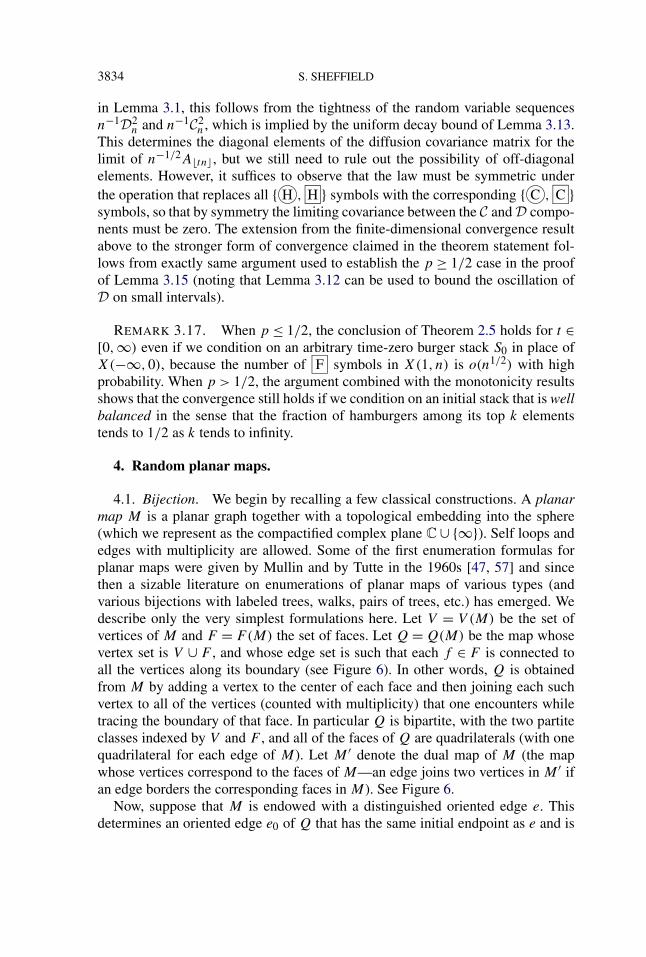
4.1. Bijection. We begin by recalling a few classical constructions. A planarmap M is a planar graph together with a topological embedding into the sphere(which we represent as the compactified complex plane C ∪ {∞}). Self loops andedges with multiplicity are allowed. Some of the first enumeration formulas forplanar maps were given by Mullin and by Tutte in the 1960s [47, 57] and sincethen a sizable literature on enumerations of planar maps of various types (andvarious bijections with labeled trees, walks, pairs of trees, etc.) has emerged. Wedescribe only the very simplest formulations here. Let V = V (M) be the set ofvertices of M and F = F(M) the set of faces. Let Q = Q(M) be the map whosevertex set is V ∪ F , and whose edge set is such that each f ∈ F is connected toall the vertices along its boundary (see Figure 6). In other words, Q is obtainedfrom M by adding a vertex to the center of each face and then joining each suchvertex to all of the vertices (counted with multiplicity) that one encounters whiletracing the boundary of that face. In particular Q is bipartite, with the two partiteclasses indexed by V and F , and all of the faces of Q are quadrilaterals (with onequadrilateral for each edge of M). Let M ′ denote the dual map of M (the mapwhose vertices correspond to the faces of M—an edge joins two vertices in M ′ ifan edge borders the corresponding faces in M). See Figure 6.
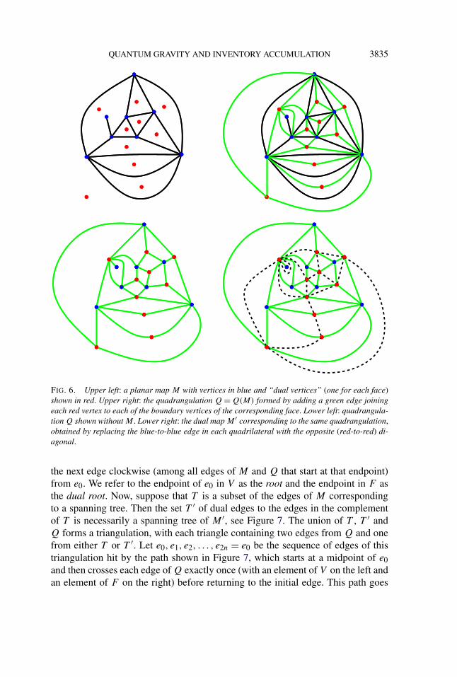
Now, suppose that M is endowed with a distinguished oriented edge e. Thisdetermines an oriented edge e0 of Q that has the same initial endpoint as e and is
QUANTUM GRAVITY AND INVENTORY ACCUMULATION 3835
FIG. 6. Upper left: a planar map M with vertices in blue and “dual vertices” (one for each face)shown in red. Upper right: the quadrangulation Q = Q(M) formed by adding a green edge joiningeach red vertex to each of the boundary vertices of the corresponding face. Lower left: quadrangula-tion Q shown without M . Lower right: the dual map M ′ corresponding to the same quadrangulation,obtained by replacing the blue-to-blue edge in each quadrilateral with the opposite (red-to-red) di-agonal.
the next edge clockwise (among all edges of M and Q that start at that endpoint)from e0. We refer to the endpoint of e0 in V as the root and the endpoint in F asthe dual root. Now, suppose that T is a subset of the edges of M correspondingto a spanning tree. Then the set T ′ of dual edges to the edges in the complementof T is necessarily a spanning tree of M ′, see Figure 7. The union of T , T ′ andQ forms a triangulation, with each triangle containing two edges from Q and onefrom either T or T ′. Let e0, e1, e2, . . . , e2n = e0 be the sequence of edges of thistriangulation hit by the path shown in Figure 7, which starts at a midpoint of e0and then crosses each edge of Q exactly once (with an element of V on the left andan element of F on the right) before returning to the initial edge. This path goes
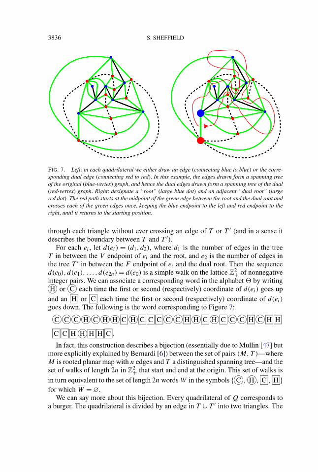
3836 S. SHEFFIELD
FIG. 7. Left: in each quadrilateral we either draw an edge (connecting blue to blue) or the corre-sponding dual edge (connecting red to red). In this example, the edges drawn form a spanning treeof the original (blue-vertex) graph, and hence the dual edges drawn form a spanning tree of the dual(red-vertex) graph. Right: designate a “root” (large blue dot) and an adjacent “dual root” (largered dot). The red path starts at the midpoint of the green edge between the root and the dual root andcrosses each of the green edges once, keeping the blue endpoint to the left and red endpoint to theright, until it returns to the starting position.
through each triangle without ever crossing an edge of T or T ′ (and in a sense itdescribes the boundary between T and T ′).
For each ei , let d(ei) = (d1, d2), where d1 is the number of edges in the treeT in between the V endpoint of ei and the root, and e2 is the number of edges inthe tree T ′ in between the F endpoint of ei and the dual root. Then the sequenced(e0), d(e1), . . . , d(e2n) = d(e0) is a simple walk on the lattice Z2+ of nonnegativeinteger pairs. We can associate a corresponding word in the alphabet � by writingH or C each time the first or second (respectively) coordinate of d(ei) goes up
and an H or C each time the first or second (respectively) coordinate of d(ei)
goes down. The following is the word corresponding to Figure 7:
C C C H C H H C H C C C C C H H C H C C C H C H H
C C H H H H C .
In fact, this construction describes a bijection (essentially due to Mullin [47] butmore explicitly explained by Bernardi [6]) between the set of pairs (M,T )—whereM is rooted planar map with n edges and T a distinguished spanning tree—and theset of walks of length 2n in Z
2+ that start and end at the origin. This set of walks is
in turn equivalent to the set of length 2n words W in the symbols { C , H , C , H }for which W =∅.
We can say more about this bijection. Every quadrilateral of Q corresponds toa burger. The quadrilateral is divided by an edge in T ∪ T ′ into two triangles. The
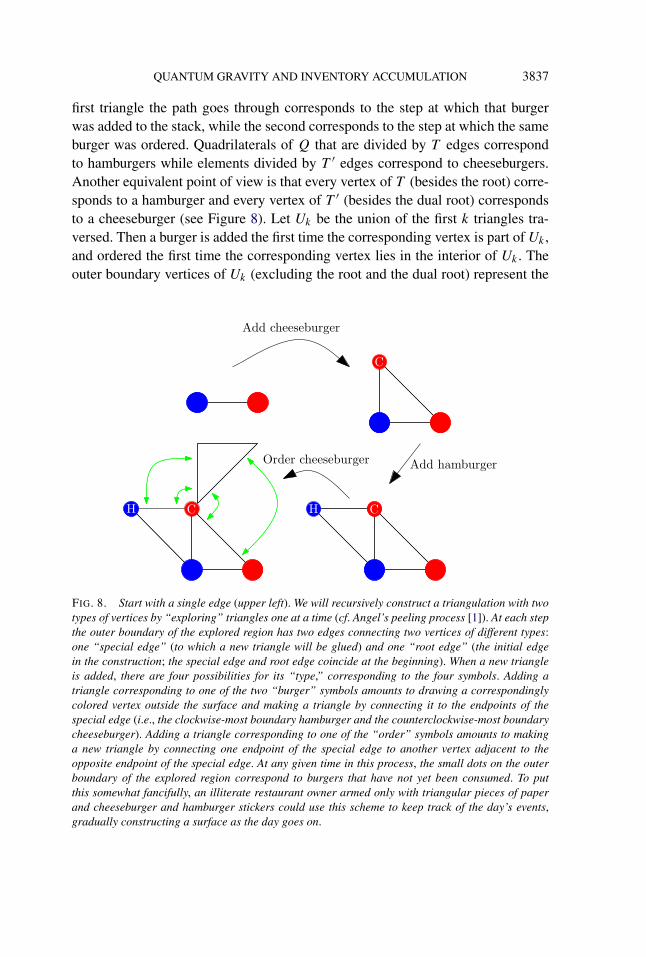
QUANTUM GRAVITY AND INVENTORY ACCUMULATION 3837
first triangle the path goes through corresponds to the step at which that burgerwas added to the stack, while the second corresponds to the step at which the sameburger was ordered. Quadrilaterals of Q that are divided by T edges correspondto hamburgers while elements divided by T ′ edges correspond to cheeseburgers.Another equivalent point of view is that every vertex of T (besides the root) corre-sponds to a hamburger and every vertex of T ′ (besides the dual root) correspondsto a cheeseburger (see Figure 8). Let Uk be the union of the first k triangles tra-versed. Then a burger is added the first time the corresponding vertex is part of Uk ,and ordered the first time the corresponding vertex lies in the interior of Uk . Theouter boundary vertices of Uk (excluding the root and the dual root) represent the
FIG. 8. Start with a single edge (upper left). We will recursively construct a triangulation with twotypes of vertices by “exploring” triangles one at a time (cf. Angel’s peeling process [1]). At each stepthe outer boundary of the explored region has two edges connecting two vertices of different types:one “special edge” (to which a new triangle will be glued) and one “root edge” (the initial edgein the construction; the special edge and root edge coincide at the beginning). When a new triangleis added, there are four possibilities for its “type,” corresponding to the four symbols. Adding atriangle corresponding to one of the two “burger” symbols amounts to drawing a correspondinglycolored vertex outside the surface and making a triangle by connecting it to the endpoints of thespecial edge (i.e., the clockwise-most boundary hamburger and the counterclockwise-most boundarycheeseburger). Adding a triangle corresponding to one of the “order” symbols amounts to makinga new triangle by connecting one endpoint of the special edge to another vertex adjacent to theopposite endpoint of the special edge. At any given time in this process, the small dots on the outerboundary of the explored region correspond to burgers that have not yet been consumed. To putthis somewhat fancifully, an illiterate restaurant owner armed only with triangular pieces of paperand cheeseburger and hamburger stickers could use this scheme to keep track of the day’s events,gradually constructing a surface as the day goes on.
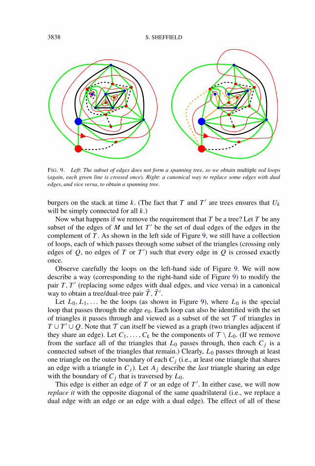
3838 S. SHEFFIELD
FIG. 9. Left: The subset of edges does not form a spanning tree, so we obtain multiple red loops(again, each green line is crossed once). Right: a canonical way to replace some edges with dualedges, and vice versa, to obtain a spanning tree.
burgers on the stack at time k. (The fact that T and T ′ are trees ensures that Uk
will be simply connected for all k.)Now what happens if we remove the requirement that T be a tree? Let T be any
subset of the edges of M and let T ′ be the set of dual edges of the edges in thecomplement of T . As shown in the left side of Figure 9, we still have a collectionof loops, each of which passes through some subset of the triangles (crossing onlyedges of Q, no edges of T or T ′) such that every edge in Q is crossed exactlyonce.
Observe carefully the loops on the left-hand side of Figure 9. We will nowdescribe a way (corresponding to the right-hand side of Figure 9) to modify thepair T ,T ′ (replacing some edges with dual edges, and vice versa) in a canonicalway to obtain a tree/dual-tree pair T , T ′.
Let L0,L1, . . . be the loops (as shown in Figure 9), where L0 is the specialloop that passes through the edge e0. Each loop can also be identified with the setof triangles it passes through and viewed as a subset of the set T of triangles inT ∪ T ′ ∪ Q. Note that T can itself be viewed as a graph (two triangles adjacent ifthey share an edge). Let C1, . . . ,Ck be the components of T \ L0. (If we removefrom the surface all of the triangles that L0 passes through, then each Cj is aconnected subset of the triangles that remain.) Clearly, L0 passes through at leastone triangle on the outer boundary of each Cj (i.e., at least one triangle that sharesan edge with a triangle in Cj ). Let Aj describe the last triangle sharing an edgewith the boundary of Cj that is traversed by L0.
This edge is either an edge of T or an edge of T ′. In either case, we will nowreplace it with the opposite diagonal of the same quadrilateral (i.e., we replace adual edge with an edge or an edge with a dual edge). The effect of all of these
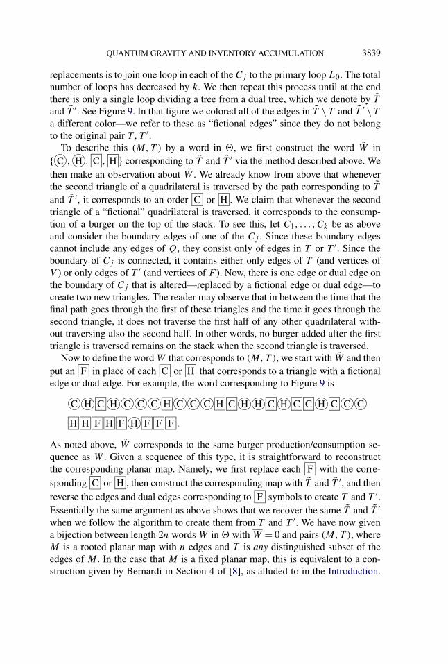
QUANTUM GRAVITY AND INVENTORY ACCUMULATION 3839
replacements is to join one loop in each of the Cj to the primary loop L0. The totalnumber of loops has decreased by k. We then repeat this process until at the endthere is only a single loop dividing a tree from a dual tree, which we denote by T
and T ′. See Figure 9. In that figure we colored all of the edges in T \ T and T ′ \ T
a different color—we refer to these as “fictional edges” since they do not belongto the original pair T ,T ′.
To describe this (M,T ) by a word in �, we first construct the word W in{ C , H , C , H } corresponding to T and T ′ via the method described above. Wethen make an observation about W . We already know from above that wheneverthe second triangle of a quadrilateral is traversed by the path corresponding to T
and T ′, it corresponds to an order C or H . We claim that whenever the secondtriangle of a “fictional” quadrilateral is traversed, it corresponds to the consump-tion of a burger on the top of the stack. To see this, let C1, . . . ,Ck be as aboveand consider the boundary edges of one of the Cj . Since these boundary edgescannot include any edges of Q, they consist only of edges in T or T ′. Since theboundary of Cj is connected, it contains either only edges of T (and vertices ofV ) or only edges of T ′ (and vertices of F ). Now, there is one edge or dual edge onthe boundary of Cj that is altered—replaced by a fictional edge or dual edge—tocreate two new triangles. The reader may observe that in between the time that thefinal path goes through the first of these triangles and the time it goes through thesecond triangle, it does not traverse the first half of any other quadrilateral with-out traversing also the second half. In other words, no burger added after the firsttriangle is traversed remains on the stack when the second triangle is traversed.
Now to define the word W that corresponds to (M,T ), we start with W and thenput an F in place of each C or H that corresponds to a triangle with a fictionaledge or dual edge. For example, the word corresponding to Figure 9 is
C H C H C C C H C C C H C H H C H C C H C C C
H H F H F H F F F .
As noted above, W corresponds to the same burger production/consumption se-quence as W . Given a sequence of this type, it is straightforward to reconstructthe corresponding planar map. Namely, we first replace each F with the corre-sponding C or H , then construct the corresponding map with T and T ′, and thenreverse the edges and dual edges corresponding to F symbols to create T and T ′.Essentially the same argument as above shows that we recover the same T and T ′when we follow the algorithm to create them from T and T ′. We have now givena bijection between length 2n words W in � with W = 0 and pairs (M,T ), whereM is a rooted planar map with n edges and T is any distinguished subset of theedges of M . In the case that M is a fixed planar map, this is equivalent to a con-struction given by Bernardi in Section 4 of [8], as alluded to in the Introduction.
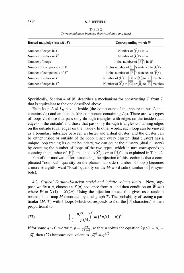
3840 S. SHEFFIELD
TABLE 2Correspondences between decorated map and word
Rooted map/edge set: (M,T ) Corresponding word: W
Number of edges in T Number of H ’s in W
Number of edges in T ′ Number of C ’s in W
Number of loops 1 plus number of F ’s in W
Number of components of T 1 plus number of F ’s matched to C ’s
Number of components of T ′ 1 plus number of F ’s matched to H ’s
Number of edges in T Number of H to H or C to F matches
Number of edges in T ′ Number of C to C or H to F matches
Specifically, Section 4 of [8] describes a mechanism for constructing T from T
that is equivalent to the one described above.Each loop L = L0 has an inside (the component of the sphere minus L that
contains L0) and an outside (the component containing L0). There are two typesof loops L: those that pass only through triangles with edges on the inside (dualedges on the outside) and those that pass only through triangles containing edgeson the outside (dual edges on the inside). In other words, each loop can be viewedas a boundary interface between a cluster and a dual cluster, and the cluster canbe either inside or outside of the loop. Since every cluster (dual cluster) has aunique loop tracing its outer boundary, we can count the clusters (dual clusters)by counting the number of loops of the two types, which in turn corresponds tocounting the number of F ’s matched to C ’s or to H ’s, as explained in Table 2.
Part of our motivation for introducing the bijection of this section is that a com-plicated “nonlocal” quantity on the planar map side (number of loops) becomesa more straightforward “local” quantity on the �-word side (number of F sym-bols).
4.2. Critical Fortuin–Kastelyn model and infinite volume limits. Now, sup-pose we fix a p, choose an X(n) sequence from μ, and then condition on W = 0where W = X(1) · · ·X(2n). Using the bijection above, this gives us a randomrooted planar map M decorated by a subgraph T . The probability of seeing a par-ticular (M,T ) with � loops (which corresponds to � of the F characters) is thenproportional to (
p/2
(1 − p)/4
)�
= (2p/(1 − p)
)�.(27)
If for some q > 0, we write p =√
q
2+√q
, so that p solves the equation 2p/(1−p) =√
q , then (27) becomes equivalent to√
q� = q�/2.
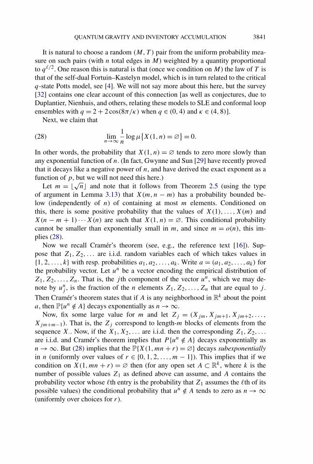
QUANTUM GRAVITY AND INVENTORY ACCUMULATION 3841
It is natural to choose a random (M,T ) pair from the uniform probability mea-sure on such pairs (with n total edges in M) weighted by a quantity proportionalto q�/2. One reason this is natural is that (once we condition on M) the law of T isthat of the self-dual Fortuin–Kastelyn model, which is in turn related to the criticalq-state Potts model, see [4]. We will not say more about this here, but the survey[32] contains one clear account of this connection [as well as conjectures, due toDuplantier, Nienhuis, and others, relating these models to SLE and conformal loopensembles with q = 2 + 2 cos(8π/κ) when q ∈ (0,4) and κ ∈ (4,8)].
Next, we claim that
limn→∞
1
nlogμ
{X(1, n) = ∅
} = 0.(28)
In other words, the probability that X(1, n) = ∅ tends to zero more slowly thanany exponential function of n. (In fact, Gwynne and Sun [29] have recently provedthat it decays like a negative power of n, and have derived the exact exponent as afunction of p, but we will not need this here.)
Let m = √n� and note that it follows from Theorem 2.5 (using the typeof argument in Lemma 3.13) that X(m,n − m) has a probability bounded be-low (independently of n) of containing at most m elements. Conditioned onthis, there is some positive probability that the values of X(1), . . . ,X(m) andX(n − m + 1) · · ·X(n) are such that X(1, n) = ∅. This conditional probabilitycannot be smaller than exponentially small in m, and since m = o(n), this im-plies (28).
Now we recall Cramér’s theorem (see, e.g., the reference text [16]). Sup-pose that Z1,Z2, . . . are i.i.d. random variables each of which takes values in{1,2, . . . , k} with resp. probabilities a1, a2, . . . , ak . Write a = (a1, a2, . . . , ak) forthe probability vector. Let un be a vector encoding the empirical distribution ofZ1,Z2, . . . ,Zn. That is, the j th component of the vector un, which we may de-note by un
j , is the fraction of the n elements Z1,Z2, . . . ,Zn that are equal to j .
Then Cramér’s theorem states that if A is any neighborhood in Rk about the point
a, then P{un /∈ A} decays exponentially as n → ∞.Now, fix some large value for m and let Zj = (Xjm,Xjm+1,Xjm+2, . . . ,
Xjm+m−1). That is, the Zj correspond to length-m blocks of elements from thesequence X·. Now, if the X1,X2, . . . are i.i.d. then the corresponding Z1,Z2, . . .
are i.i.d. and Cramér’s theorem implies that P {un /∈ A} decays exponentially asn → ∞. But (28) implies that the P{X(1,mn + r) = ∅} decays subexponentiallyin n (uniformly over values of r ∈ {0,1,2, . . . ,m − 1}). This implies that if wecondition on X(1,mn + r) = ∅ then (for any open set A ⊂ R
k , where k is thenumber of possible values Z1 as defined above can assume, and A contains theprobability vector whose �th entry is the probability that Z1 assumes the �th of itspossible values) the conditional probability that un /∈ A tends to zero as n → ∞(uniformly over choices for r).

3842 S. SHEFFIELD
From this, we may conclude that if one chooses X(1) · · ·X(N) conditionedon X(1,N) = ∅ and then picks a random k and recenters the sequence at X(k),then one obtains a sequence of random recentered processes whose infinite vol-ume limit is a random process with law μ. In this sense, μ describes an infinitevolume limit of the critical Fortuin–Kastelyn models. Given a sequence X(·) sam-pled from μ, the corresponding sequence Y(·) can be then used to construct aninfinite random surface with an infinite spanning tree and spanning dual tree (inthe manner described above for finite words). From this perspective, Theorem 2.5can be understood a scaling limit result about this random pair of infinite trees(which in turn encode the structure of a random infinite planar map).
APPENDIX: BACKGROUND: CONTEXT AND MOTIVATION
We now say a bit more about the larger project that motivated this work, namely,the problem of relating discrete random surfaces to continuum objects like Li-ouville quantum gravity, conformal loop ensembles, and the Schramm–Loewnerevolution.
A longstanding open physics-motivated problem is to show that as the num-ber of edges in the random maps described here tends to infinity, the correspond-ing loop-decorated surfaces (appropriately rescaled) converge in law to a limitingloop-decorated random surface M. The physics literature provides ample heuris-tic evidence, in various settings, for the existence of a phase transition analogousto the p = 1/2 transition we present: p > 1/2 corresponds to what is called thebranched polymer (a.k.a. continuum random tree) phase, while p < 1/2 is the Li-ouville quantum gravity phase. The literature is too vast for us to properly surveyhere, but sample works in this direction include [3, 9–11, 13–15, 17, 18, 23, 24,31, 34, 35, 56]. This paper presents a clear and rigorous illustration of the phasetransition.
The p > 1/2 case is relatively simple. Applying Theorem 2.5 when p > 1/2 wesee that in the scaling limit, the spanning tree and the dual spanning tree that weconstruct converge in law to a.s. identical continuum random trees. The collectionof quadrilaterals corresponding to the tree and the collection corresponding to thedual tree can each be interpreted as approximations of the same continuum randomtree: gluing the two together produces a surface that, as a metric space, shouldapproximate the same tree. [Note that since X(−∞, n) corresponds to a branchof a tree and X(n,∞) a branch of the corresponding dual tree, Proposition 3.8implies that when we glue these surfaces together a positive fraction of the pointsalong any branch of the tree or dual tree correspond to length-one loops that are“bottlenecks” of the combined surface. We do not know whether this remains truewhen p = 1/2.]
The p < 1/2 case is more interesting. Based on various theorems and heuristics,we expect the limiting surface M to be a Liouville quantum gravity (LQG) surfacedecorated by a conformal loop ensemble (CLE), with respective parameters γ and
QUANTUM GRAVITY AND INVENTORY ACCUMULATION 3843
κ depending on q . Precise formulations of this conjecture, along with definitionsof LQG surfaces (whose laws depend on a parameter γ ) and CLEs (whose lawsdepend on a parameter κ , and are based on the Schramm–Loewner evolution withparameter κ), can be found in [21, 22, 52, 53] (along with much more extensivelists of references; the CLEs relevant to this paper have a parameter κ ∈ (4,8],while the κ ≤ 4 case is discussed in [54]). But in a sense this question has beenaround since the 1980s when Polyakov first introduced Liouville quantum gravity[48, 49] (see also [33]).
Polyakov writes in a recent memoir [50] that he first became convinced of theconnection between the discrete models and Liouville quantum gravity after jointlyderiving, with Knizhnik and Zamolodchikov, the KPZ formula for so-called LQGscaling dimensions and comparing these dimensions with known combinatorialresults for the discrete models [33]. The KPZ formula was recently proved math-ematically in [20, 21] and can indeed be interpreted as evidence for the conver-gence conjectures. But actually proving these conjectures, even in a physics sense,remains a challenge.
There are various ways to formulate a convergence statement, depending onwhat topology one uses when talking about convergence in law [52]. One approachis to consider a model without loops and to interpret the discrete surfaces as ran-dom metric spaces. If one uses the Gromov–Hausdorff topology on metric spaces,then recent independent works by Miermont and Le Gall show that these metricspaces converge in law to a limiting random metric space called the Brownian map[39, 44]. Prior to these recent works, it was known that these discrete random met-ric spaces converge in law to limiting random metric spaces along subsequences,and that any subsequential limit is a random metric space that is almost surelyhomeomorphic to the sphere; see [37, 38, 41, 43], as well as the recent survey[40]. The Brownian map is conjecturally equivalent, as a metric space, to an LQGsurface with γ = √
8/3 [52].4 So far, there has been little success in extendingthe metric space theory to more general FK-weighted random surfaces, which arebelieved to correspond to other values of γ .
Another approach to the convergence problem is to ignore metric space struc-ture and focus instead on conformal structure. In this case, one may consider aconformal map from a random discretized surface to the sphere, and then studythe induced area measure on the sphere and the images of the loops on the sphere.The conformal point of view plays a central role in the physics literature on Liou-ville quantum gravity and “random metrics”, which has been developed as part ofa general subject called conformal field theory. (In this literature, the term “met-ric” refers most directly to a Riemannian metric tensor, not a two-point distance
4One barrier to establishing this equivalence is that it remains an open question even to show thatLQG surfaces have a canonical metric space structure. There is an obvious way to define a two-pointdistance function on an LQG surface in terms of limits, as explained in a footnote in [52], but it hasnot been proved that these limits exist and are nontrivial.
3844 S. SHEFFIELD
function.) Various precise conjectures along these lines are presented in [21, 52],along with a more extensive bibliography.
This paper takes a third approach. We encode loop-decorated surfaces by walkson Z
2 (“inventory trajectories”). Roughly speaking, the loops determine a canoni-cal non-self-intersecting “exploration path” which goes through every face on thesurface and more or less traces all the loops. This path divides the surface into a“tree” and a “dual tree”—and the exploration driving function encodes the struc-ture of this pair of trees. If we consider a topology in which two loop-decoratedsurfaces are considered close when their exploration driving functions are close,then Theorem 2.5 can be interpreted as a scaling limit result for the random sur-faces. It describes the limiting law of the pair of trees and the manner in whichthey are glued together. (Note: the symmetry between the tree and dual tree makesour approach very different from the version of the Schaeffer bijection [51] usedto define the Brownian map [40]. The latter involves a breadth-first search treewith geodesic branches and a dual tree that looks completely different from thetree itself—in particular, its diameter scales like a different power of the numberof edges.)
It turns out that if one replaces discrete loops with a continuum CLE, then theloops determine a continuum (space-filling) analog of the “exploration path” de-scribed above, which traces through all of the loops in a canonical way [45, 53].We can interpret this continuum exploration process as tracing the boundary be-tween a continuum (space-filling) tree and a continuum (space-filling) dual tree.If one draws these trees on a Liouville quantum gravity random surface, then thelengths of branches of the tree are well defined a.s. by the results of [52], so thatone can construct a continuum analog of the exploration driving function describedin this paper.
As mentioned in the Introduction, since this paper was originally posted thearXiv there have been several additional papers that have extended the theory de-veloped here. One recently completed work with Bertrand Duplantier and JasonMiller [19] demonstrates that LQG surfaces decorated by CLEs indeed have well-defined exploration driving functions themselves, and that their laws are those ofprecisely the same kinds of Brownian motions as long as the parameters p,q, κ, γ
are matched up correctly.5 As in the discrete case, the continuum exploration driv-ing function should encode the metric space structure of a certain tree (here acontinuum random tree) and a dual-tree. The simplest case is when κ = 8, corre-sponding to the case p = 0. The results of this paper are trivial (following fromthe classical central limit theorem for simple random walks) in that case, but theLiouville quantum gravity construction is still interesting.
5Specifically, p ∈ [0,1/2), q ∈ [0,4), κ ∈ (4,8], γ ∈ [√2,2) and q = 2 + 2 cos 8πκ , γ = √
16/κ ,
p =√
q
2+√q
.
QUANTUM GRAVITY AND INVENTORY ACCUMULATION 3845
As explained in [19], this program allows us to interpret the results presentedhere to mean that the discrete loop-decorated surfaces of this paper converge toCLE-decorated Liouville quantum gravity in a topology where two configurationsare close if the corresponding driving functions are close. Extensions of this resultto stronger topologies (which encode lengths and intersection locations of loopconfigurations) have been established in works by (various subsets of) Cheng Mao,Ewain Gwynne, Jason Miller, and Xin Sun [27–30]. See also the related results in[5, 12].
Moving from this kind of convergence to convergence in topologies that moredirectly encode the metric space and/or conformal structure of the random surfacesthemselves appears difficult, but conceivably possible. One way to do this would beto show that if one couples a discrete loop-decorated surface with a CLE-decoratedLQG surface in such a way that their driving functions are likely to be close, thenit is likely that the two surfaces are also in some sense close as metric spaces, oras Riemannian manifolds with a conformal structure. We expect statements of thiskind to be true, but proving them will require new ideas.
Since we would ultimately like to extend the results presented here to othertopologies, we conclude with one relevant question. If two discrete loop-decoratedsurfaces M1 and M2 are conditioned to have exploration driving functions thatare close in the L∞ sense for all time, is it then the case that (with high prob-ability) one can conformally map M1 to M2 in such a way that the image ofthe exploration path in M1 is close to the exploration path in M2 (at least on afixed compact interval of time)? This question is already interesting in the casethat p = 0. The results by Gill and Rohde in [26] about Brownian motion on theserandom surfaces, and the parabolicity of the infinite volume surfaces, constitute apromising step in this direction.
Acknowledgments. We thank Olivier Bernardi, Bertrand Duplantier, EwainGwynne, Nike Sun, Xin Sun, and Sam Watson for very helpful comments on draftsof this paper. We thank an anonymous referee for proposing many improvementsthat were incorporated into the text.
REFERENCES
[1] ANGEL, O. (2003). Growth and percolation on the uniform infinite planar triangulation. Geom.Funct. Anal. 13 935–974. MR2024412
[2] AZUMA, K. (1967). Weighted sums of certain dependent random variables. Tôhoku Math. J.(2) 19 357–367. MR0221571
[3] BAILLIE, C. F. and JOHNSTON, D. A. (1992). Multiple Potts models coupled to two-dimensional quantum gravity. Phys. Lett. B 286 44–52.
[4] BAXTER, R. J., KELLAND, S. B. and WU, F. Y. (1976). Equivalence of the Potts model orWhitney polynomial with an ice-type model. J. Phys. A: Math. Gen. 9 397.
[5] BERESTYCKI, N., LASLIER, B. and RAY, G. (2015). Critical exponents on Fortuin–Kastelynweighted planar maps. Preprint. Available at arXiv:1502.00450.
3846 S. SHEFFIELD
[6] BERNARDI, O. (2007). Bijective counting of tree-rooted maps and shuffles of parenthesis sys-tems. Electron. J. Combin. 14 Research Paper 9, 36 pp. (electronic). MR2285813
[7] BERNARDI, O. (2008). A characterization of the Tutte polynomial via combinatorial embed-dings. Ann. Comb. 12 139–153. MR2428901
[8] BERNARDI, O. (2008). Tutte polynomial, subgraphs, orientations and sandpile model:New connections via embeddings. Electron. J. Combin. 15 Research Paper 109, 53.MR2438581
[9] BERNARDI, O. and BOUSQUET-MÉLOU, M. (2011). Counting colored planar maps: Alge-braicity results. J. Combin. Theory Ser. B 101 315–377. MR2802884
[10] BOROT, G. and EYNARD, B. (2011). Enumeration of maps with self-avoiding loops and theO(n) model on random lattices of all topologies. J. Stat. Mech. Theory Exp. 1 P01010,62. MR2770626
[11] CATES, M. E. (1988). The Liouville field theory of random surfaces: When is the bosonicstring a branched polymer? EPL (Europhysics Letters) 7 719.
[12] CHEN, L. (2015). Basic properties of the infinite critical-FK random map. Preprint. Availableat arXiv:1502.01013.
[13] DAUL, J.-M. (1995). Q-States Potts model on a random planar lattice. Preprint. Available atarXiv:hep-th/9502014.
[14] DAVID, F. (1985). Planar diagrams, two-dimensional lattice gravity and surface models. Nu-clear Phys. B 257 45–58. MR0788098
[15] DAVID, F. (1997). A scenario for the c > 1 barrier in non-critical bosonic strings. NuclearPhys. B 487 633–649. MR1432821
[16] DEMBO, A. and ZEITOUNI, O. (2010). Large Deviations Techniques and Applications.Stochastic Modelling and Applied Probability 38. Springer, Berlin. MR2571413
[17] DUPLANTIER, B. and KOSTOV, I. (1988). Conformal spectra of polymers on a random surface.Phys. Rev. Lett. 61 1433–1437. MR0960093
[18] DUPLANTIER, B. and KOSTOV, I. K. (1990). Geometrical critical phenomena on a randomsurface of arbitrary genus. Nuclear Phys. B 340 491–541. MR1068092
[19] DUPLANTIER, B., MILLER, J. and SHEFFIELD, S. (2014). Liouville quantum gravity as amating of trees. Preprint. Available at arXiv:1409.7055.
[20] DUPLANTIER, B. and SHEFFIELD, S. (2009). Duality and the Knizhnik–Polyakov–Zamolodchikov relation in Liouville quantum gravity. Phys. Rev. Lett. 102 150603, 4.MR2501276
[21] DUPLANTIER, B. and SHEFFIELD, S. (2011). Liouville quantum gravity and KPZ. Invent.Math. 185 333–393. MR2819163
[22] DUPLANTIER, B. and SHEFFIELD, S. (2011). Schramm–Loewner evolution and Liouvillequantum gravity. Phys. Rev. Lett. 107 131305.
[23] EYNARD, B. (2011). Formal matrix integrals and combinatorics of maps. In Random Matrices,Random Processes and Integrable Systems. 415–442. Springer, New York. MR2858440
[24] EYNARD, B. and BONNET, G. (1999). The Potts-q random matrix model: Loop equations,critical exponents, and rational case. Phys. Lett. B 463 273–279. MR1722272
[25] GEORGII, H.-O. (2011). Gibbs Measures and Phase Transitions, 2nd ed. de Gruyter Studiesin Mathematics 9. de Gruyter, Berlin. MR2807681
[26] GILL, J. T. and ROHDE, S. (2013). On the Riemann surface type of random planar maps. Rev.Mat. Iberoam. 29 1071–1090. MR3090146
[27] GWYNNE, E., MAO, C. and SUN, X. (2015). Scaling limits for the critical Fortuin–Kasteleynmodel on a random planar map I: Cone times. Preprint. Available at arXiv:1502.00546.
[28] GWYNNE, E. and MILLER, J. (2015). Convergence of the topology of critical Fortuin–Kasteleyn planar maps to that of CLEκ on a Liouville quantum surface. In preparation.
QUANTUM GRAVITY AND INVENTORY ACCUMULATION 3847
[29] GWYNNE, E. and SUN, X. (2015). Scaling limits for the critical Fortuin–Kastelyn model ona random planar map II: Local estimates and empty reduced word exponent. Preprint.Available at arXiv:1505.03375.
[30] GWYNNE, E. and SUN, X. (2015). Scaling limits for the critical Fortuin–Kastelyn model on arandom planar map III: Finite volume case. In preparation.
[31] HARRIS, G. (1994). Percolation on strings and the cover-up of the c = 1 disaster. NuclearPhys. B 418 278–304. MR1281359
[32] KAGER, W. and NIENHUIS, B. (2004). A guide to stochastic Löwner evolution and its appli-cations. J. Stat. Phys. 115 1149–1229. MR2065722
[33] KNIZHNIK, V. G., POLYAKOV, A. M. and ZAMOLODCHIKOV, A. B. (1988). Fractal structureof 2D-quantum gravity. Modern Phys. Lett. A 3 819–826. MR0947880
[34] KOSTOV, I. K. (1989). O(n) vector model on a planar random lattice: Spectrum of anomalousdimensions. Modern Phys. Lett. A 4 217–226. MR1016518
[35] KOSTOV, I. K. (1989). The ADE face models on a fluctuating planar lattice. Nuclear Phys. B326 583–612. MR1028516
[36] LE GALL, J.-F. (1995). The Brownian snake and solutions of �u = u2 in a domain. Probab.Theory Related Fields 102 393–432. MR1339740
[37] LE GALL, J.-F. (2007). The topological structure of scaling limits of large planar maps. Invent.Math. 169 621–670. MR2336042
[38] LE GALL, J.-F. (2010). Geodesics in large planar maps and in the Brownian map. Acta Math.205 287–360. MR2746349
[39] LE GALL, J.-F. (2013). Uniqueness and universality of the Brownian map. Ann. Probab. 412880–2960. MR3112934
[40] LE GALL, J.-F. and MIERMONT, G. (2012). Scaling limits of random trees and planar maps.In Probability and Statistical Physics in Two and More Dimensions. Clay Math. Proc. 15155–211. Amer. Math. Soc., Providence, RI. MR3025391
[41] LE GALL, J.-F. and PAULIN, F. (2008). Scaling limits of bipartite planar maps are homeomor-phic to the 2-sphere. Geom. Funct. Anal. 18 893–918. MR2438999
[42] MAO, C., SUN, X. and ZHOU, T. (2014). Inventory accumulation with k products. In prepara-tion.
[43] MIERMONT, G. (2008). On the sphericity of scaling limits of random planar quadrangulations.Electron. Commun. Probab. 13 248–257. MR2399286
[44] MIERMONT, G. (2013). The Brownian map is the scaling limit of uniform random plane quad-rangulations. Acta Math. 210 319–401. MR3070569
[45] MILLER, J. and SHEFFIELD, S. (2013). Imaginary geometry IV: Interior rays, whole-planereversibility, and space-filling trees. Preprint. Available at arXiv:1302.4738.
[46] MILLER, J. and SHEFFIELD, S. (2015). Liouville quantum gravity spheres as matings of finite-diameter trees. Preprint. Available at arXiv:1506.03804.
[47] MULLIN, R. C. (1967). On the enumeration of tree-rooted maps. Canad. J. Math. 19 174–183.MR0205882
[48] POLYAKOV, A. M. (1981). Quantum geometry of bosonic strings. Phys. Lett. B 103 207–210.MR0623209
[49] POLYAKOV, A. M. (1981). Quantum geometry of fermionic strings. Phys. Lett. B 103 211–213.MR0623210
[50] POLYAKOV, A. M. (2008). From Quarks to Strings. Preprint. Available at arXiv:0812.0183.[51] SCHAEFFER, G. (1997). Bijective census and random generation of Eulerian planar maps with
prescribed vertex degrees. Electron. J. Combin. 4 Research Paper 20, 14 pp. (electronic).MR1465581
[52] SHEFFIELD, S. (2005). Conformal weldings of random surfaces: SLE and the quantum gravityzipper. Preprint. Available at arXiv:1012.4797.
3848 S. SHEFFIELD
[53] SHEFFIELD, S. (2009). Exploration trees and conformal loop ensembles. Duke Math. J. 14779–129. MR2494457
[54] SHEFFIELD, S. and WERNER, W. (2012). Conformal loop ensembles: The Markovian charac-terization and the loop-soup construction. Ann. of Math. (2) 176 1827–1917. MR2979861
[55] SUN, X. and WILSON, D. B. (2015). Sandpiles and unicycles on random planar maps. Preprint.Available at arXiv:1506.08881.
[56] THORLEIFSSON, G. (1993). Coupling of multiple q-state Potts models to 2d gravity. In Pro-ceedings of the International Symposium on Nuclear Physics B—Proceedings Supple-ments 30 787–790.
[57] TUTTE, W. T. (1968). On the enumeration of planar maps. Bull. Amer. Math. Soc. 74 64–74.MR0218276
DEPARTMENT OF MATHEMATICS
MASSACHUSETTS INSTITUTE OF TECHNOLOGY
77 MASSACHUSETTS AVENUE
CAMBRIDGE, MASSACHUSETTS 02139USAE-MAIL: [email protected]