Embed Size (px)
Citation preview
Quantum Haar Wavelet Transformsand Their Applications
Darwin Gosal∗ and Wayne Lawton†
National University of Singapore, Singapore 119260
November 5, 2001
Fourier transform has been shown to be a powerful tool in many area ofscience. However, there is another class of unitary transforms, the wavelettransforms, which are as useful as the Fourier transform. Wavelet transformsare used to expose the multi-scale structure of a signal and very useful forimage processing and data compression. In this paper, we construct quantumalgorithms for Haar wavelet transforms and show its application in analyzingthe multi-scale structure of the dynamical system by the Logistic Map (x→λx(1− x)), where λ takes value in the interval [0, 4).
1 Introduction
Information is stored, transmitted and processed by physical means 1. Thus,the concept of information and computation can be formulated in the contextof a physical theory and the study of information requires experimentation.This sentence leads to non-trivial consequences in the world of quantummechanics.
The field of quantum information science has undergone explosive activ-ity over the past few years. This quantum information science has generatedthree great developments in the latter part of the 20th century, they arequantum computation, quantum cryptography, and quantum error correc-tion. These three developments in quantum information science all posegreat challenges for both 21st century science and technology.
Quantum Computation not only fascinates physicists, it also interestscomputer scientists and mathematicians. For computer scientist, quantum∗Email: [email protected]†Email: [email protected] what Rolf Landauer said “Information is physical”
1
computation introduces new complexity classes that can transform some NP-Complete problems to the Polynomial complexity.
Several quantum algorithms are known, the most famous example isDeutsch’s algorithm for deciding whether a function is even or balanced.One of the most remarkable quantum algorithms is Shor’s algorithm. Thisalgorithm basically depends on quantum Fourier transform (QFT). As weknow the Fourier transform is good for analyzing the periodicity of a func-tion, but wavelet transform is able to analyze the multiscale structure of thefunction.
It is sufficient to use some basic empirically-based principles of quantumbehavior in order to explain the basic principles of Quantum Computing andto develop quantum algorithms. In order to formulate these principles weneed to introduce some basic concepts.
2 Quantum Mechanics
Quantum theory is a mathematical model of the physical world. To charac-terize the model, we need to specify how it represents: states, observables,measurement, and dynamics.
2.1 Axioms of quantum mechanics
Quantum mechanics is a mathematical framework for the development ofphysical theories. On its own quantum mechanics doesn’t tell you whatlaws a physical system must obey, but it does provide a mathematical andconceptual framework for the development of such laws. Therefore, we needsome axioms to provide a connection between the physical world and themathematical formalism of quantum mechanics.
States Associated to any isolated physical system is a complex vector spacewith inner product (that is, a Hilbert space2) known as the state spaceof the system. The system is completely described by its state vec-tor, which is a unit vector in the system’s state space. In short, astate vector (which is a ray in a Hilbert space) can be thought of asthe mathematical representative of the physical notion of ‘state’ of thesystem.
Observables An observable is a property of a physical system that in prin-ciple can be measured.The observables of the system can be represented
2which I will elaborate more on the next subsection
2
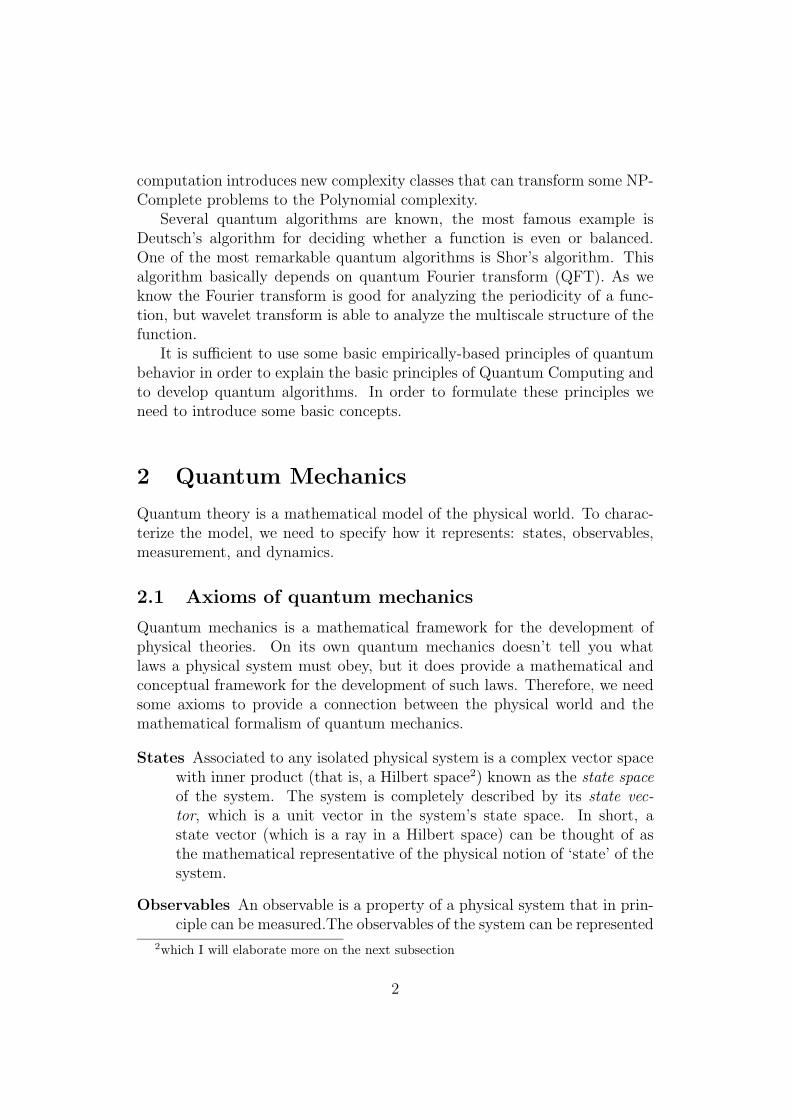
mathematically by self-adjoint operator that act on the Hilbert spaceH. An operator is a linear map taking vectors to vectors
A : |ψ〉 → A|ψ〉,A (a|ψ〉+ b|ψ〉) = aA|ψ〉+ bA|ψ〉 (1)
A is self-adjoint3 if and only if A = A†.
Measurement Quantum measurements are described by a collection {Mm}of measurement operators. These are operators acting on the statespace of the system being measured. The index m refers to the mea-surement outcomes that may occur in the experiment. If the state ofthe quantum system is |ψ〉 immediately before the measurement thenthe probability that result m occurs is given by
P (m) = 〈ψ|M†mMm|ψ〉 (2)
and the state of the system after measurement is
Mm|ψ〉√〈ψ|M†
mMm|ψ〉. (3)
The measurement operators satisfy the completeness equation,
∑m
M†mMm = I (4)
The completeness equation expresses the fact that probabilities sum toone.
Dynamics The evolution of a closed quantum system is described by aunitary transformation. That is, the state |ψ〉 of the system at timet1 is related to the state |ψ′〉 of the system at time t2 by a unitaryoperator U which depends only on the times t1 and t2,
|ψ′〉 = U|ψ〉. (5)
The time evolution of the state of a closed quantum system is describedby the Schrodinger equation,
3or Hermitian
3
i~d|ψ〉dt
= H|ψ〉. (6)
where H is a fixed Hermitian operator knowns as the Hamiltonian ofthe closed system. In the case where H is t-independent; it can beshown that U = e−itH.
This completes the mathematical formulation of quantum mechanics.Further reading on the foundation of quantum mechanics can be found on [8].A very useful bibliographic guide to the foundations of quantum mechanicsand quantum information can be found on [11].
2.2 Hilbert space
In this subsection I will define Hilbert spacesH that furnishes the mathemat-ical basis for the treatment of quantum mechanics in terms of those conceptswhich are subsequently needed in quantum mechanics.
Hilbert space is a vector space over complex numbers C. In the following Ishall denote the points of Hilbert space by |φ〉, |χ〉, |ψ〉, . . ., complex numbersby a, b, c, . . ., and positive integers by i, j, k, . . ..
These are the five Hilbert spaces axioms:
First axiom A linear vector space S, with a carrier H, over a field K withthe carrier K is an algebra S = 〈H,+,−1 ,0, K,+f ,×f , 0, 1, ·〉 such that〈H,+,−1 ,0〉 is a commutative group, K = 〈K,+f ,×f , 0, 1〉 is a field,and · : K × H → H is a scalar multiplication satisfying the followingaxioms for any a, b ∈ K, |φ〉, |ψ〉, and |χ〉 ∈ H:
• Commutative law of addition
|ψ〉+ |φ〉 = |φ〉+ |ψ〉
• Associative law of addition
(|φ〉+ |ψ〉) + |χ〉 = |φ〉+ (|ψ〉+ |χ〉)
• Distributive law of multiplication
(a+f b)|ψ〉 = a · |ψ〉+ b · |ψ〉a · (|φ〉+ |ψ〉) = a · |φ〉+ a · |ψ〉
4
• Associative law of multiplication
(a×f b) · |ψ〉 = a · (b · |ψ〉)
• Role of 0 and 1
0 · |ψ〉 = 0 ; 1 · |ψ〉 = |ψ〉
Second axiom A complex inner-product space H is a vector space with acarrier H over the field of complex numbers, equipped with an innerproduct (also called scalar product or Hermitian scalar product) 〈·|·〉 :H×H → C satisfying, for any |φ〉, |ψ〉, and |χ〉 ∈ H, and any c1, c2 ∈ C,the following properties:
• Hermitian symmetry
〈ψ|φ〉 = 〈φ|ψ〉∗
• Definite form
〈ψ|ψ〉 ≥ 0 and 〈ψ|ψ〉 = 0 if and only if |ψ〉 = 0
• Associative and distributive law
〈ψ|c1φ+ c2χ〉 = c1〈ψ|φ〉+ c2〈ψ|χ〉
The inner product introduces on H the norm ‖ψ‖H =√〈ψ|ψ〉 and the
distance between ψ and φ is ‖ψ − φ‖.
Third axiom There are arbitrarily many linearly independent vectors. thatis, for each k = 1, 2, . . . , we can specify k such vectors.
Fourth axiom An inner-product space H is complete. That is, if for anysequence {|ψi〉}∞i=1 in H satisfies the Cauchy convergence criterion (foreach ε > 0, there exist an N = N(ε), such that ‖ψm − ψn‖ < ε for allm,n ≥ N), then it is convergent. A complete inner-product space iscalled a Hilbert space.
Fifth axiom H is separable. That is, there is a sequence |ψ1〉, |ψ2〉, . . . in Hwhich is everywhere dense in H.
5
Note:To each continuous linear mapping f : H → C, the Riesz representation
theorem ensure that there exists a unique φf ∈ H such that f(ψ) = 〈φf |ψ〉for any ψ ∈ H. The space of all linear mapping (called also functionals) ofa Hilbert space H forms again a Hilbert space, called dual Hilbert space (orconjugate Hilbert space). The mapping fφ(ψ) = 〈φ|ψ〉 is a functional for anyφ ∈ H. Thus a bra-vector 〈·| can be seen as the operator that maps eachstate φ into a functional 〈φ| such that 〈φ|(|ψ〉) = 〈φ|ψ〉 for every state.
A rigorous mathematical treatment for Hilbert space can be found on [9]
2.3 The density matrix
The axioms of quantum mechanics that discussed in the subsection 2.1 pro-vide a perfectly acceptable general formulation of the quantum theory. Thetrouble is that our axioms are intended to characterize the quantum behaviorof the entire universe. In practice, the observations are always limited to asmall part of a much larger quantum system. When we limit our attentionto just part of a larger system, then:
1. States are not rays.
2. Measurements are not orthogonal projections.
3. Evolution is not unitary.
We can best understand these points by considering the bipartite systemor a system that undergoes decoherence. Therefore, states that are not pureare called mixed states.
Consider a mixed state ρ := (|ψ1〉, |ψ2〉, . . . , |ψn〉; p1, p2, . . . , pn) where∑ni=1 pi = 1. Let A be any operator. Now let |ψ〉 in H. Then
〈A〉ψ = 〈ψ|A|ψ〉 =N∑j=1
〈ψ|A|ej〉〈ej|ψ〉 ≡N∑j=1
〈ej|ψ〉〈ψ|A|ej〉
=N∑j=1
〈ej|ρψA|ej〉 = Tr(ρψA) (7)
where ρψ := |ψ〉〈ψ|Now define the mixed-state operator ρ by
ρ ≡∑i
pi|ψi〉〈ψi| (8)
The operator ρ has the following properties:
6
1. ρ is self-adjoint: ρ = ρ†
2. ρ is a positive, semi-definite operator: 〈ψ|ρ|ψ〉 ≥ 0 for all |ψ〉
3. Tr(ρ) = 1
It follows that ρ can be diagonalized, that the eigenvalues are all realand non-negative, and that the eigenvalues sum up to one. In general, anyoperator satisfying these three conditions is called a density matrix. Notethat a pure density matrix has the property ρ2 = ρ. Hence, the densitymatrix ρ is a “generalization” of the notion of state and it represent all andonly information which can be learned by sampling the ensemble.
3 Quantum Computation and Information
Quantum computation and quantum information is the study of the informa-tion processing tasks that can be accomplished using quantum mechanicalsystems that we described earlier. Two key problems here are: how to rep-resent information and how to manipulate quantum information.
3.1 Qubits and entanglement
The most fundamental concept of classical computation and classical infor-mation is bit (binary digit). This is a system that can take on one of twovalues, such as true and false or 0 and 1. Qubit (Quantum bit) is the quantumanalog of a bit. Just as a classical bit, it has two states.
LetH be a two-dimensional quantum system with two orthonormal states,denoted by |0〉 and |1〉, that can be considered as forming standard basis ofH. A qubit is a quantum state
|ψ〉 = α|0〉+ β|1〉 (9)
where α, β ∈ C and |α|2 + |β|2 = 1.One picture useful in thinking about qubits is the following representa-
tion.
|ψ〉 = cosθ
2|0〉+ eiϕ sin
θ
2|1〉 (10)
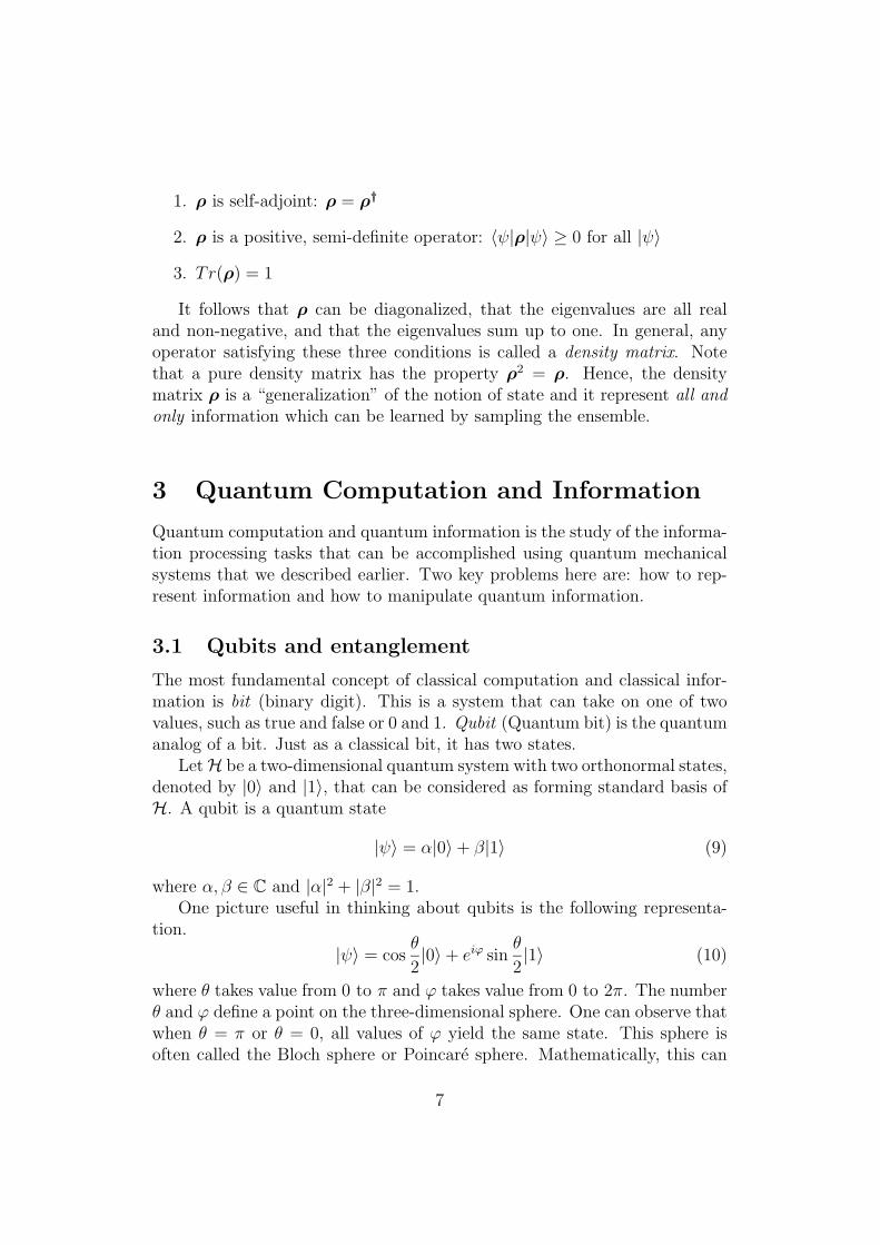
where θ takes value from 0 to π and ϕ takes value from 0 to 2π. The numberθ and ϕ define a point on the three-dimensional sphere. One can observe thatwhen θ = π or θ = 0, all values of ϕ yield the same state. This sphere isoften called the Bloch sphere or Poincare sphere. Mathematically, this can
7
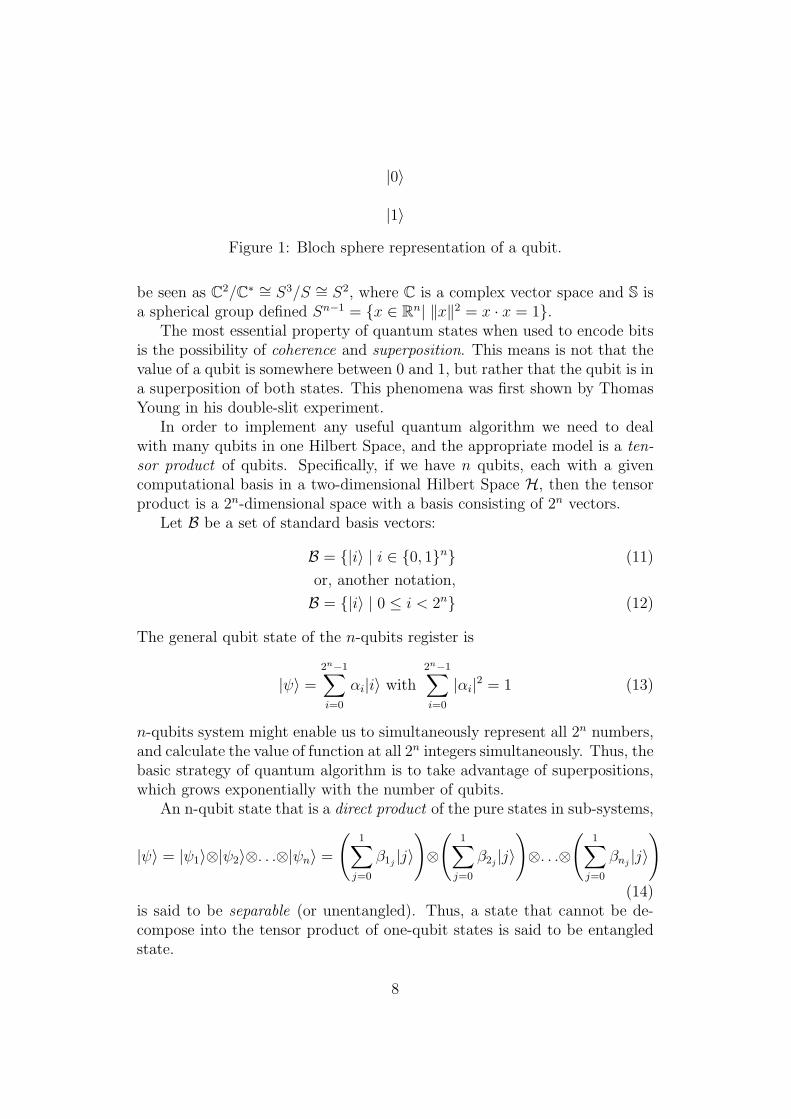
|0〉
|1〉
Figure 1: Bloch sphere representation of a qubit.
be seen as C2/C∗ ∼= S3/S ∼= S2, where C is a complex vector space and S isa spherical group defined Sn−1 = {x ∈ Rn| ‖x‖2 = x · x = 1}.
The most essential property of quantum states when used to encode bitsis the possibility of coherence and superposition. This means is not that thevalue of a qubit is somewhere between 0 and 1, but rather that the qubit is ina superposition of both states. This phenomena was first shown by ThomasYoung in his double-slit experiment.
In order to implement any useful quantum algorithm we need to dealwith many qubits in one Hilbert Space, and the appropriate model is a ten-sor product of qubits. Specifically, if we have n qubits, each with a givencomputational basis in a two-dimensional Hilbert Space H, then the tensorproduct is a 2n-dimensional space with a basis consisting of 2n vectors.
Let B be a set of standard basis vectors:
B = {|i〉 | i ∈ {0, 1}n} (11)
or, another notation,
B = {|i〉 | 0 ≤ i < 2n} (12)
The general qubit state of the n-qubits register is
|ψ〉 =2n−1∑i=0
αi|i〉 with2n−1∑i=0
|αi|2 = 1 (13)
n-qubits system might enable us to simultaneously represent all 2n numbers,and calculate the value of function at all 2n integers simultaneously. Thus, thebasic strategy of quantum algorithm is to take advantage of superpositions,which grows exponentially with the number of qubits.
An n-qubit state that is a direct product of the pure states in sub-systems,
|ψ〉 = |ψ1〉⊗|ψ2〉⊗. . .⊗|ψn〉 =
(1∑j=0
β1j |j〉
)⊗
(1∑j=0
β2j |j〉
)⊗. . .⊗
(1∑j=0
βnj |j〉
)(14)
is said to be separable (or unentangled). Thus, a state that cannot be de-compose into the tensor product of one-qubit states is said to be entangledstate.
8
An important example of entangled states is the Bell state or EPR pair,i.e.
|Φ+〉 =1√2
(|00〉+ |11〉) (15)
This innocuous-looking state is responsible for a remarkable phenomenacalled non-locality and is at the heart of EPR (Einstein-Podolsky-Rosen)paradox. The set of Bell states (Ψ± and Φ±) is the key ingredient in quantumteleportation and super-dense coding. A further reading on entanglement canbe found in [10], [5], and [3]
3.2 Quantum Gates
Classical computer circuits consist of wires and logic gates. In a similar way,quantum computer have a quantum gates from which quantum computingdevices are designed.
Quantum gates on a n-qubit can be described by a 2n by 2n matrices.Because of the normalization condition requires
∑2n−1i=0 |αi|2 = 1, there is a
constrain for matrices that can be used as quantum gates. It turns out thatthe appropriate condition is that the matrix U describing the quantum gatemust be unitary, that is U†U = I. The implication of this, is that a unitaryoperation implies a reversible operation.
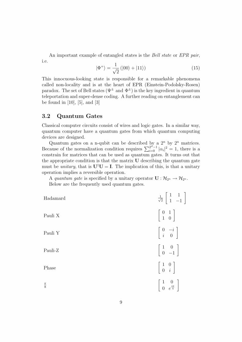
A quantum gate is specified by a unitary operator U : H2n → H2n .Below are the frequently used quantum gates.
Hadamard 1√2
[1 11 −1
]
Pauli X
[0 11 0
]
Pauli Y
[0 −ii 0
]
Pauli-Z
[1 00 −1
]
Phase
[1 00 i
]π8
[1 0
0 eiπ4
]
9
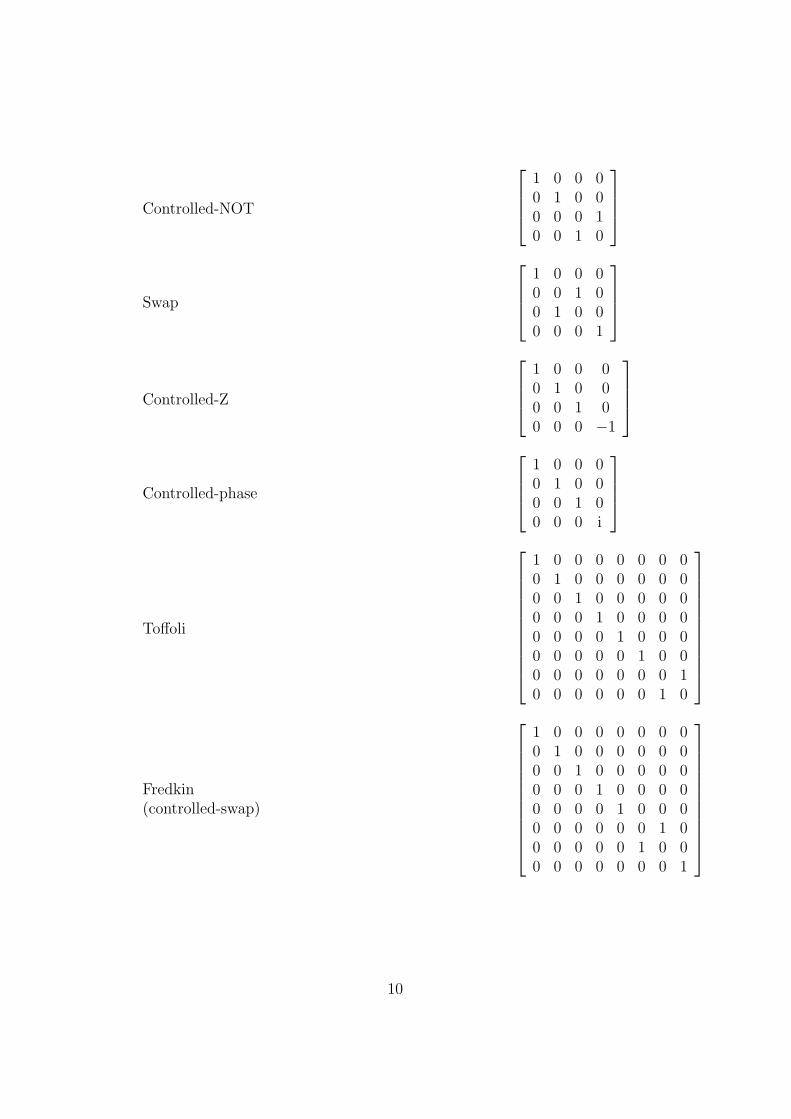
Controlled-NOT
1 0 0 00 1 0 00 0 0 10 0 1 0
Swap
1 0 0 00 0 1 00 1 0 00 0 0 1
Controlled-Z
1 0 0 00 1 0 00 0 1 00 0 0 −1
Controlled-phase
1 0 0 00 1 0 00 0 1 00 0 0 i
Toffoli
1 0 0 0 0 0 0 00 1 0 0 0 0 0 00 0 1 0 0 0 0 00 0 0 1 0 0 0 00 0 0 0 1 0 0 00 0 0 0 0 1 0 00 0 0 0 0 0 0 10 0 0 0 0 0 1 0
Fredkin(controlled-swap)
1 0 0 0 0 0 0 00 1 0 0 0 0 0 00 0 1 0 0 0 0 00 0 0 1 0 0 0 00 0 0 0 1 0 0 00 0 0 0 0 0 1 00 0 0 0 0 1 0 00 0 0 0 0 0 0 1
10
3.3 Quantum Circuits
Quantum circuit is a collection of quantum gates acyclicly4 connected by“quantum wires”5. There are few features allowed in classical circuits thatare not present in quantum circuits. First of all, classical circuits allow wiresto be ’joined’ together, an operation known as fanin. Secondly, the inverseoperation, fanout whereby several copies of a bit is produced, is also notallowed in quantum circuits.
The size and the depth of a circuit refer to the number of nodes anddepth of the underlying connection graph. The circuit is to be read from theleft-to-right. It is conventional to assume that the state input to the circuit isa computational basis state, usually the state consisting of all |0〉’s. We shallfind quantum circuits useful as models of all quantum processes, includingbut not limited to computation, communication, and even quantum noise.
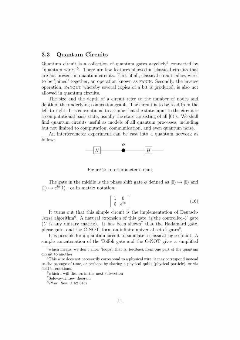
An interferometer experiment can be cast into a quantum network asfollow:
H H
φx
Figure 2: Interferometer circuit
The gate in the middle is the phase shift gate φ defined as |0〉 7→ |0〉 and|1〉 7→ eiφ|1〉 , or in matrix notation,[
1 00 eiφ
](16)
It turns out that this simple circuit is the implementation of Deutsch-Jozsa algorithm6. A natural extension of this gate, is the controlled-U gate(U is any unitary matrix). It has been shown7 that the Hadamard gate,phase gate, and the C-NOT, form an infinite universal set of gates8.
It is possible for a quantum circuit to simulate a classical logic circuit. Asimple concatenation of the Toffoli gate and the C-NOT gives a simplified
4which means, we don’t allow ’loops’, that is, feedback from one part of the quantumcircuit to another
5This wire does not necessarily correspond to a physical wire; it may correspond insteadto the passage of time, or perhaps by sharing a physical qubit (physical particle), or viafield interactions.
6which I will discuss in the next subsection7Solovay-Kitaev theorem8Phys. Rev. A 52 3457
11
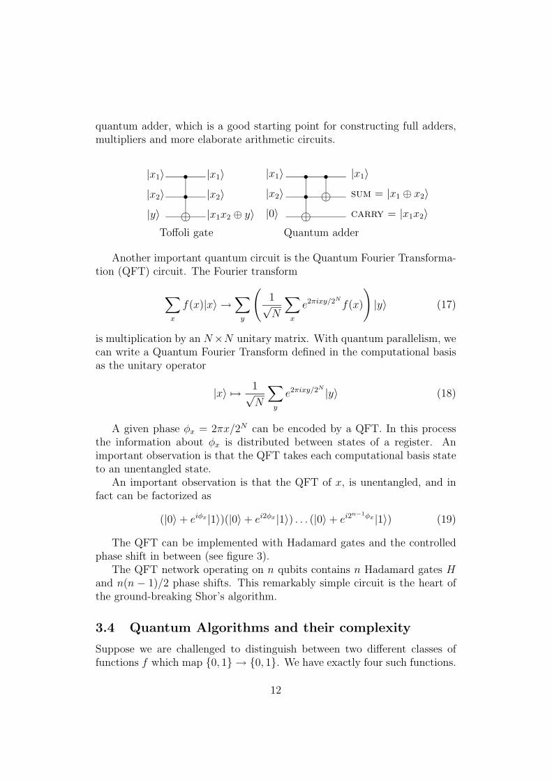
quantum adder, which is a good starting point for constructing full adders,multipliers and more elaborate arithmetic circuits.
|x1〉
|x2〉
|y〉
ssh|x1〉
|x2〉
|x1x2 ⊕ y〉
|x1〉
|x2〉
|0〉
|x1〉
sum = |x1 ⊕ x2〉
carry = |x1x2〉
sshsh
Toffoli gate Quantum adder
Another important quantum circuit is the Quantum Fourier Transforma-tion (QFT) circuit. The Fourier transform
∑x
f(x)|x〉 →∑y
(1√N
∑x
e2πixy/2Nf(x)
)|y〉 (17)
is multiplication by an N×N unitary matrix. With quantum parallelism, wecan write a Quantum Fourier Transform defined in the computational basisas the unitary operator
|x〉 7→ 1√N
∑y
e2πixy/2N |y〉 (18)
A given phase φx = 2πx/2N can be encoded by a QFT. In this processthe information about φx is distributed between states of a register. Animportant observation is that the QFT takes each computational basis stateto an unentangled state.
An important observation is that the QFT of x, is unentangled, and infact can be factorized as
(|0〉+ eiφx|1〉)(|0〉+ ei2φx|1〉) . . . (|0〉+ ei2n−1φx|1〉) (19)
The QFT can be implemented with Hadamard gates and the controlledphase shift in between (see figure 3).
The QFT network operating on n qubits contains n Hadamard gates Hand n(n − 1)/2 phase shifts. This remarkably simple circuit is the heart ofthe ground-breaking Shor’s algorithm.
3.4 Quantum Algorithms and their complexity
Suppose we are challenged to distinguish between two different classes offunctions f which map {0, 1} → {0, 1}. We have exactly four such functions.
12
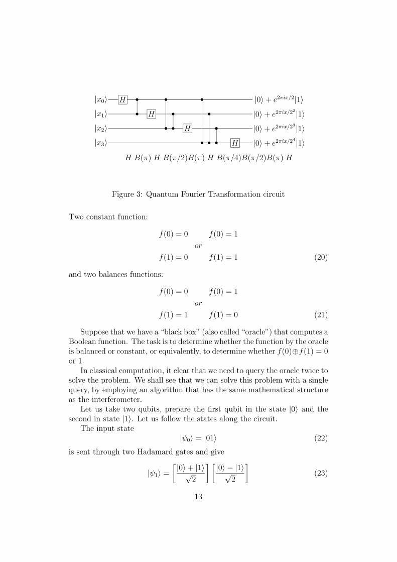
|x3〉
|x2〉
|x1〉
|x0〉
|0〉+ e2πix/24|1〉
|0〉+ e2πix/23|1〉
|0〉+ e2πix/22|1〉
|0〉+ e2πix/2|1〉
H B(π) H B(π/2)B(π) H B(π/4)B(π/2)B(π) H
H
H
H
H sssssss s s
sss
Figure 3: Quantum Fourier Transformation circuit
Two constant function:
f(0) = 0 f(0) = 1
or
f(1) = 0 f(1) = 1 (20)
and two balances functions:
f(0) = 0 f(0) = 1
or
f(1) = 1 f(1) = 0 (21)
Suppose that we have a “black box” (also called “oracle”) that computes aBoolean function. The task is to determine whether the function by the oracleis balanced or constant, or equivalently, to determine whether f(0)⊕f(1) = 0or 1.
In classical computation, it clear that we need to query the oracle twice tosolve the problem. We shall see that we can solve this problem with a singlequery, by employing an algorithm that has the same mathematical structureas the interferometer.
Let us take two qubits, prepare the first qubit in the state |0〉 and thesecond in state |1〉. Let us follow the states along the circuit.
The input state|ψ0〉 = |01〉 (22)
is sent through two Hadamard gates and give
|ψ1〉 =
[|0〉+ |1〉√
2
] [|0〉 − |1〉√
2
](23)
13
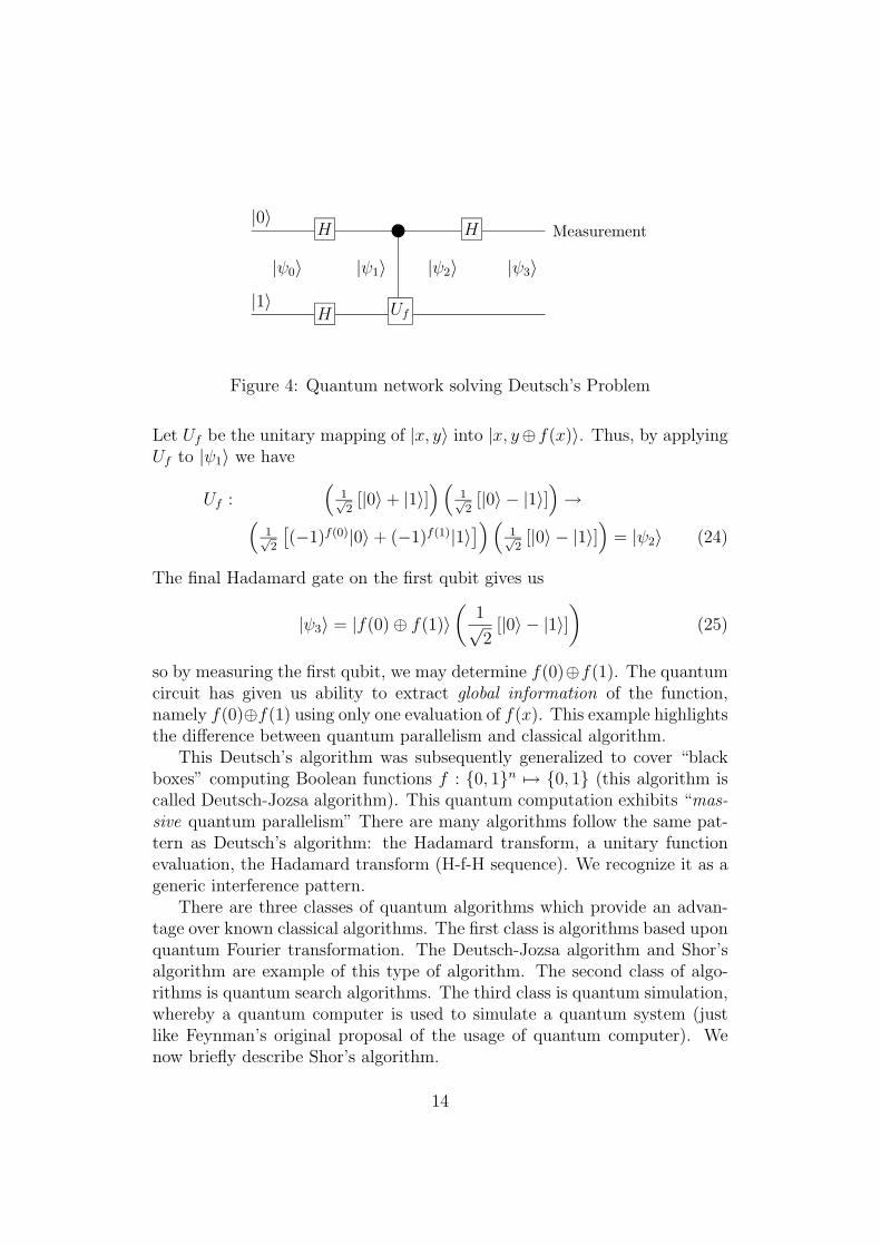
Measurement
|1〉
|0〉
|ψ0〉 |ψ1〉 |ψ2〉 |ψ3〉
x
UfH
H H
Figure 4: Quantum network solving Deutsch’s Problem
Let Uf be the unitary mapping of |x, y〉 into |x, y⊕f(x)〉. Thus, by applyingUf to |ψ1〉 we have
Uf :(
1√2
[|0〉+ |1〉])(
1√2
[|0〉 − |1〉])→(
1√2
[(−1)f(0)|0〉+ (−1)f(1)|1〉
]) (1√2
[|0〉 − |1〉])
= |ψ2〉 (24)
The final Hadamard gate on the first qubit gives us
|ψ3〉 = |f(0)⊕ f(1)〉(
1√2
[|0〉 − |1〉])
(25)
so by measuring the first qubit, we may determine f(0)⊕f(1). The quantumcircuit has given us ability to extract global information of the function,namely f(0)⊕f(1) using only one evaluation of f(x). This example highlightsthe difference between quantum parallelism and classical algorithm.
This Deutsch’s algorithm was subsequently generalized to cover “blackboxes” computing Boolean functions f : {0, 1}n 7→ {0, 1} (this algorithm iscalled Deutsch-Jozsa algorithm). This quantum computation exhibits “mas-sive quantum parallelism” There are many algorithms follow the same pat-tern as Deutsch’s algorithm: the Hadamard transform, a unitary functionevaluation, the Hadamard transform (H-f-H sequence). We recognize it as ageneric interference pattern.
There are three classes of quantum algorithms which provide an advan-tage over known classical algorithms. The first class is algorithms based uponquantum Fourier transformation. The Deutsch-Jozsa algorithm and Shor’salgorithm are example of this type of algorithm. The second class of algo-rithms is quantum search algorithms. The third class is quantum simulation,whereby a quantum computer is used to simulate a quantum system (justlike Feynman’s original proposal of the usage of quantum computer). Wenow briefly describe Shor’s algorithm.
14
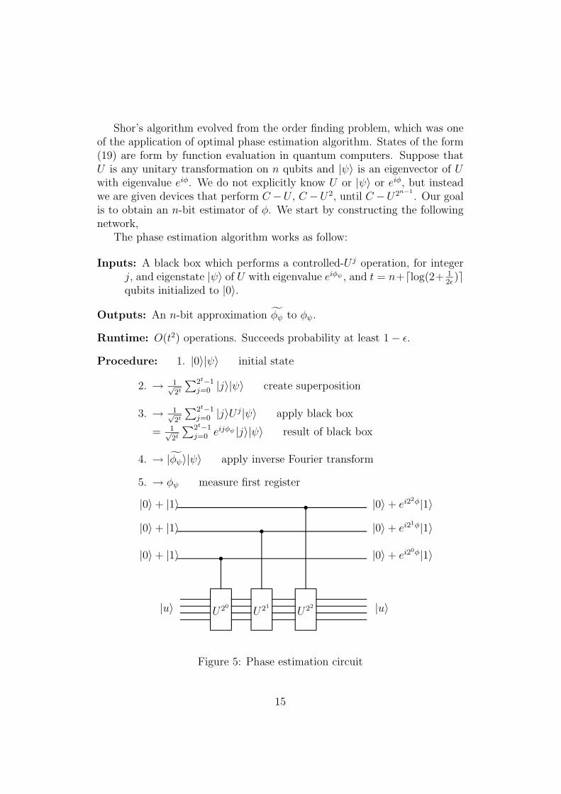
Shor’s algorithm evolved from the order finding problem, which was oneof the application of optimal phase estimation algorithm. States of the form(19) are form by function evaluation in quantum computers. Suppose thatU is any unitary transformation on n qubits and |ψ〉 is an eigenvector of Uwith eigenvalue eiφ. We do not explicitly know U or |ψ〉 or eiφ, but insteadwe are given devices that perform C −U , C −U2, until C −U2n−1
. Our goalis to obtain an n-bit estimator of φ. We start by constructing the followingnetwork,
The phase estimation algorithm works as follow:
Inputs: A black box which performs a controlled-U j operation, for integerj, and eigenstate |ψ〉 of U with eigenvalue eiφψ , and t = n+dlog(2+ 1
2ε)e
qubits initialized to |0〉.
Outputs: An n-bit approximation φψ to φψ.
Runtime: O(t2) operations. Succeeds probability at least 1− ε.
Procedure: 1. |0〉|ψ〉 initial state
2. → 1√2t
∑2t−1j=0 |j〉|ψ〉 create superposition
3. → 1√2t
∑2t−1j=0 |j〉U j|ψ〉 apply black box
= 1√2t
∑2t−1j=0 eijφψ |j〉|ψ〉 result of black box
4. → |φψ〉|ψ〉 apply inverse Fourier transform
5. → φψ measure first register
U20U21
U22|u〉 |u〉
|0〉+ |1〉
|0〉+ |1〉
|0〉+ |1〉
|0〉+ ei20φ|1〉
|0〉+ ei21φ|1〉
|0〉+ ei22φ|1〉
sss
Figure 5: Phase estimation circuit
15
This algorithm can be applied to make quantum order-finding algorithm,which is the heart of Shor’s factoring algorithm.
The quantum order-finding algorithm work as follow:
Inputs: A black-box Ux,N which performs the transformation |j〉|k〉 → |j〉|xjk mod N〉,for x co-prime to L-bit numbers N , t = 2L + 1 + dlog(2 + 1
2ε)e qubits
initialized to |0〉, and L qubits initialized to the state |1〉.
Outputs: The least integer r > 0 such that xr = 1( mod N).
Runtime: O(L3) operations. Succeeds with probability O(1).
Procedure: 1. |0〉|1〉 initial state
2. → 1√2t
∑2t−1j=0 |j〉|1〉 create superposition
3. → 1√2t
∑2t−1j=0 |j〉|xj mod N〉 apply Ux,N
≈ 1√r2t
∑r−1s=0
∑2t−1j=0 eisj/r|j〉|ψs〉
4. → 1√r
∑r−1s=0 |s/r〉|ψs〉 apply inverse Fourier transform to first
register
5. → s/r measure first register
6. → r apply continued fractions algorithm
It has been shown that a factoring problem can be reduced to order-finding problem. The Shor’s algorithm can be summarized as follow:
Inputs: A composite number N
Outputs: A non-trivial factor of N
Runtime: O(log3 N) operations. Succeeds with probability O(1).
Procedure: 1. If n is even, return the factor 2.
2. Determine whether N = ab for integers a ≥ 1 and b ≥ 2, and ifso return the factor a
3. Randomly choose x in the range 1 to N − 1. If gcd(x,N) > 1then return the factor gcd(x,N).
4. Use order-finding subroutine to find the order r of x modulo N .
16
5. If r is even and xr/2 6= −1 (mod N) then compute gcd(xr/2−1, N)and gcd(xr/2 +1, N), and test to see if one of these is a non-trivialfactor, returning that factor if so. Otherwise, the algorithm fails.
More of quantum algorithms can be found in [4], [13], [15], and [6]. Webresources on Quantum information can be found in: http://www.qubit.organd http://www.physics.nus.edu.sg/ phyohch/hyperqc2.htm.
4 Wavelet
4.1 General characteristic of wavelets
Data as a bit (binary digit) is just a mathematical representation for thecomputation. But in our daily life, what we see is continuous wave. Thereforewe need to make this into a digital signal and analyse it. A wave is usuallydefined as an oscillating function of time or space, such as a sinusoid.
There are three ways to transform (or analyse) this signals:
1. by Fourier transform. This method expands signals in terms of cosinewaves, which has proven to be extremely important for periodic, time-invariant, or stationary phenomena. The practicality problem of thismethod is that, it need many frequencies for a high-fidelity signal.
2. into short time Fourier transform. Short segments of the signals aretransformed separately. In each segment, the signal is expanded intocosine wave as before. The disadvantage of this method is there aresudden breaks between segments (“blocking effect”).
3. into wavelets. A wavelet is a “small wave” that start and stop. It hasenergy concentrated in time, which useful to analyze transient, non-stationary, or time-varying phenomena. All wavelets come from onebasic wavelet ψ(t).
A signal f(t) can be expressed as a linear decomposition by
f(t) =∑l
alψl(t) (26)
The series representation of f in (26) is called a wavelet series. If the expan-sion (26) is unique, the set is called a basis for the class of functions. If thebasis is orthogonal, meaning
〈ψk(t)|ψl(t)〉 =
∫ψk(t)ψl(t) = 0 k 6= l (27)
17

then the coefficients can be calculated by the inner product
ak = 〈f(t)|ψk(t)〉 =
∫f(t)ψk(t)dt. (28)
For wavelet expansion, a two-parameter system is constructed such that (26)becomes
f(t) =∑k
∑j
aj,kψj,k(t) (29)
The ψj,k(t) are the wavelet expansion functions that usually form an orthogo-nal basis. The set of expansion coefficients aj,k are called the discrete wavelettransform (DWT) of f(t).
The wavelet expansion set is not unique, but all seem to have the followinggeneral characteristics:
1. A wavelet system is a set of building block to construct or represent asignal or function. It is a two-dimensional expansion set for some classof one-(or higher) dimensional signals.
2. The wavelet expansion gives a time-frequency localization of the sig-nal. This means most of the energy of the signal of the signal is wellrepresented by a few expansion coefficients.
3. The calculation of the coefficients from the signal can be done ef-ficiently. It turns out that many wavelet transforms can be calcu-lated with O(N) operations. More general wavelet transforms requireO(N log(N)) operations, the same as for the FFT.
4. All wavelet systems are generated from a single scaling function orwavelet by simple binary scaling(i.e. dilation by 2j) and dyadic trans-lation (of k/2j). The two-dimensional parameterization is achievedfrom the generating wavelet ψ(t) by
ψj,k(t) = 2j/2ψ(2jt− k) j, k ∈ Z (30)
5. Almost all useful wavelet systems also satisfy the multi-resolution con-ditions. This means that if a set of signals can be represented by aweighted sum of (t − k), then a larger set (including the original) canbe represented by a weighted sum of ϕ(2t− k).
6. The lower resolution coefficients can be calculated from higher reso-lution coefficients by a tree-structured algorithm called a filter bank.Filter bank is a set of linear time-invariant operator.
18
Before going any further, we will see the connection between filter banksand wavelets, and you will see that the high-pass filter leads to ψ(t) and thelow-pass filter leads to scaling function ϕ(t).
4.2 Filter banks
Filter bank is a set of filters. The analysis bank often has two filters, low-pass and high-pass. They separate input signal into frequency bands. Thosesub-signals can be compressed much more efficiently than the original signal.A filter is a linear time-invariant operator that acts on input vector x andgives an output vector y which is the convolution of x with a fixed vector h.The vector h contains the filter coefficients.
y(n) =∑k
h(k)x(n− k) = h ∗ x (convolution in the time domain) (31)
4.2.1 Low-pass Filter / Moving Average
We go forward by introducing the simplest low-pass filter. Low-pass filterhas its output at time t = n as the average of the input x(n) and the inputx(n− 1):
y(n) =1
2x(n) + 1
2x(n−1) (32)
The filter coefficients are h(0) = 12
and h(1) = 12. It is a moving average,
because the output averages the current component with the previous one.
4.2.2 High-pass Filter / Moving Difference
High-pass filter has its output at time t = n as the difference of the inputx(n) and the input x(n− 1):
y(n) = 12x(n)− 1
2x(n−1) (33)
The filter coefficients are h(0) = 12
and h(1) =− 12. It is a moving difference.
4.3 Scaling function and wavelets
Corresponding to the low-pass filter, there is a continuous-time scaling func-tion ϕ(t). The dilation equation for the scaling function ϕ(t) is
ϕ(t) = 2N∑k=0
h(k)ϕ(2t− k) (34)
19
Corresponding to the high-pass filter, there is a continuous-time scalingfunction wavelet ψ(t). It is a direct equation that gives ψ(t) immediatelyand explicitly from ϕ(t):
ψ(t) = 2∑
h1(k)φ(2t− k) (35)
4.4 Haar wavelet
In our example, ϕ(t) is a box function and its dilations ϕ(2t − k) are halfboxes, then the wavelet is:
ψ(t) = 2∑
h1(k)φ(2t− k) (36)
Explicitly, ψ(t) = 1 for 0 ≤ t < 12
and ψ(t) = −1 for 12≤ t < 1. This is the
Haar wavelet.Length 2 Haar wavelet can be represented as:
1√2
[1 11 −1
](37)
A sequence with length � 2, can be calculated faster with fast wavelettransform (FWT). Fast wavelet transform is a tree-structured filter bank.The algorithm of FWT can be found on the appendix9.
A more rigorous mathematical approach can be found on [16], [17], [18],and [19]. More resource on wavelet can be found on the web:http://www.amara.com/current/wavelet.html.
5 Quantum Haar Wavelet
Transition for “classical” wavelet transform to quantum wavelet transformcan be approached by factoring the classical operators for the transformationinto direct sums, direct products, and dot products of unitary matrices. Indoing so, we will find that permutation matrices play a vital role.
Two fundamental permutation matrices for quantum haar transform arethe perfect shuffle Π2n and the bit reversal P2n .
Description of the matrix Π2n in terms of its element Πij can be given as
Πij =
{1 if j = 1/2 and i is even, or if j = (i− 1)/2 + 2n−1 and i is odd0 otherwise
(38)
9fwt.m
20
As noted by Hoyer, a quantum description of Π2n can be given by
Π2n : |an−1an−2 · · · a1a0〉 7→ |a0an−1an−2 · · · a1〉 (39)
Here we can see that a swap gate Π4 is a special case of permutation matrix.Description of the matrix P2n in terms of its element Pij can be given as
Πij =
{1 if j is bit reversal of i0 otherwise
(40)
A quantum description of P2n can be given by
P2n : |an−1an−2 · · · a1a0〉 7→ |a0a1 · · · an−2an−1〉 (41)
P2n can be factorized in terms of Π2i and Π2i can be factorized in termof Π4. From previous section we know that the swap gate can be made by 2CNOT gates. Therefore the whole permutation matrices can be implementon the quantum computer.
Based on recursive definition of Haar matrices, we can factorize H2n as
H2n = (I2n−1 ⊗W ) · · · (I2n−i ⊗W ⊕ I2n−2n−i+1) · · · (W ⊕ I2n−2)×(Π4I2n−4) · · · (Π2iI2n−2i) · · · (Π2n−1I2n−1)Π2n (42)
where W is the Hadamard matrix.More on the Quantum wavelet transform can be found on [1] and [2].
6 Logistic Mapping
Chaotic dynamics was made popular by the computer experiments of RobertMay and Mitchell Feigenbaum on a mapping known as the logistic map.The remarkable feature of the logistic map is in the simplicity of its form(quadratic) and the complexity of its dynamics. It is the simplest modelthat shows chaos. Through logistic map Feigenbaum number was discovered.It is the limit of the ratio between one bifurcation and the next, in logisticmapping; the same number turns up in various chaotic systems, it is about4.669.
The logistic map is the simplest model in population dynamics that incor-porates the effects of both birth and death rates. It is given by the formula:
xn+1 = f(xn) = λ · xn · (1− xn) (43)
where the function f is called the logistic mapping and the parameter λmodels the effective growth rate. The population size, (xn) at the nth year, is
21
defined relative to the maximum population size the ecosystem can sustainand is therefore a number between 0 and 1. The parameter λ is also restrictedbetween 0 and 4 to keep the system bounded and therefore the model willmake physical sense.
The logistic equation gives the rule for determining the relative populationxn+1 at the (n+1)th year in terms of the population in the nth year. To get aphysical understanding of the terms in the the logistic equation, we can thinkof the λ ·xn term as a positive feedback term in the sense that as xn increasesso does the value of b xn. This is same as saying that the population size inthe next year (xn+1) is determined by the product of the previous populationsize xn and the rate λ at which the population grows. Similarly, the term(1 − xn) can be thought of as a negative feedback, since increasing xn willdecrease (1 − xn) and therefore (1 − xn) can be thought of as populationdecline due to over population and scarce resources. Logistic mapping is thesimplest one dimensional, nonlinear (x squared term), single parameter λmodel that shows an amazing variety of dynamical response.
The graph corresponding to the logistic function y = λ · x · (1 − x) is aparabola which passes through the points (0,0) and (1,0) independent of thechoice of the parameter λ. The maxima of the parabola, which is alwayslocated at x = 0.5, is 0.25 · λ. There is a nice graphical visualization of theiteration process of logistic map via what is called the graphical iterationplot which shows how the iterates x0, x1, x2, . . . can be obtained graphically.
It is clear that for values of λ between [0,1], if we start iterating theequation with any value of x the value of x will settle down to 0. This canbe understood from the fact that the the logistic equation is a product ofthree numbers, namely, λ, xn and (1− xn) which are all between [0,1], x atthe next time step must always be smaller than what is at the current timestep. The point zero is called the fixed point of the system and is stable forλ = [0, 1].
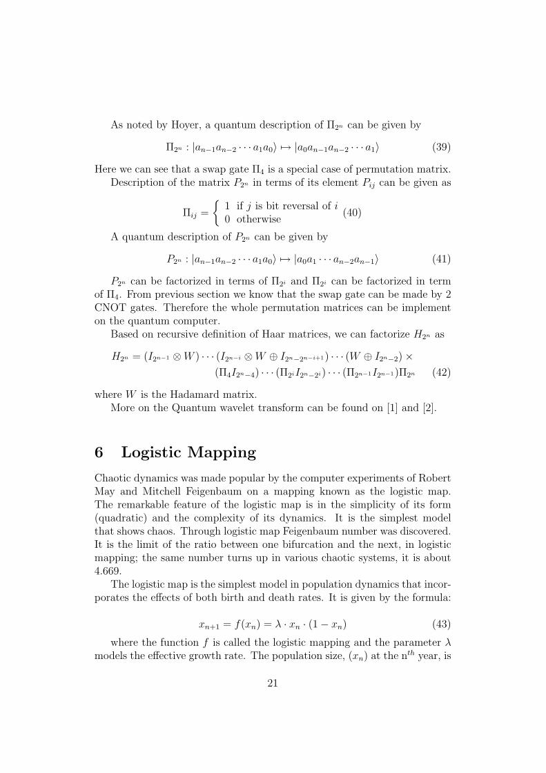
For values of λ between (1,3) the iterates instead of being attracted tozero, get attracted to a different fixed point. A fixed point is a point whichwhen fed back into the map gives back the same point. Mathematically, thisis expressed by the condition x = λ · x · (1− x). The long term behavior ofthe logistic equation when λ ≥ 3, show that the system settles down to aperiod ≥ 2 limit cycle. Figure 6 shows that the initial x attracted to a singlenon-zero fixed point.
The existence of n period limit cycle is established by real solutions to
Figure 6: Iteration with x0 = 0.2, and λ = 2.8
22
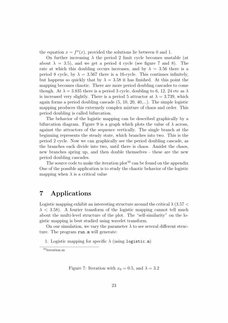
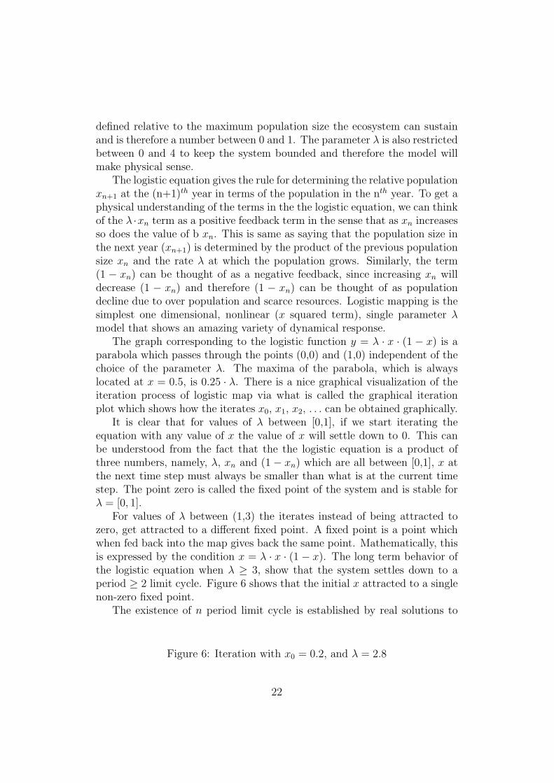
the equation x = fn(x), provided the solutions lie between 0 and 1.On further increasing λ the period 2 limit cycle becomes unstable (at
about λ = 3.5), and we get a period 4 cycle (see figure 7 and 8). Therate at which this doubling occurs increases, and by λ = 3.56 there is aperiod 8 cycle, by λ = 3.567 there is a 16-cycle. This continues infinitely,but happens so quickly that by λ = 3.58 it has finished. At this point themapping becomes chaotic. There are more period doubling cascades to comethough. At λ = 3.835 there is a period 3 cycle, doubling to 6, 12, 24 etc as λis increased very slightly. There is a period 5 attractor at λ = 3.739, whichagain forms a period doubling cascade (5, 10, 20, 40,...). The simple logisticmapping produces this extremely complex mixture of chaos and order. Thisperiod doubling is called bifurcation.
The behavior of the logistic mapping can be described graphically by abifurcation diagram. Figure 9 is a graph which plots the value of λ across,against the attractors of the sequence vertically. The single branch at thebeginning represents the steady state, which branches into two. This is theperiod 2 cycle. Now we can graphically see the period doubling cascade, asthe branches each divide into two, until there is chaos. Amidst the chaos,new branches spring up, and then double themselves - these are the newperiod doubling cascades.
The source code to make the iteration plot10 can be found on the appendixOne of the possible application is to study the chaotic behavior of the logisticmapping when λ is a critical value
7 Applications
Logistic mapping exhibit an interesting structure around the critical λ (3.57 <λ < 3.58). A fourier transform of the logistic mapping cannot tell muchabout the multi-level structure of the plot. The “self-similarity” on the lo-gistic mapping is best studied using wavelet transform.
On our simulation, we vary the parameter λ to see several different struc-ture. The program run.m will generate:
1. Logistic mapping for specific λ (using logistic.m)
10iteration.m
Figure 7: Iteration with x0 = 0.5, and λ = 3.2
23
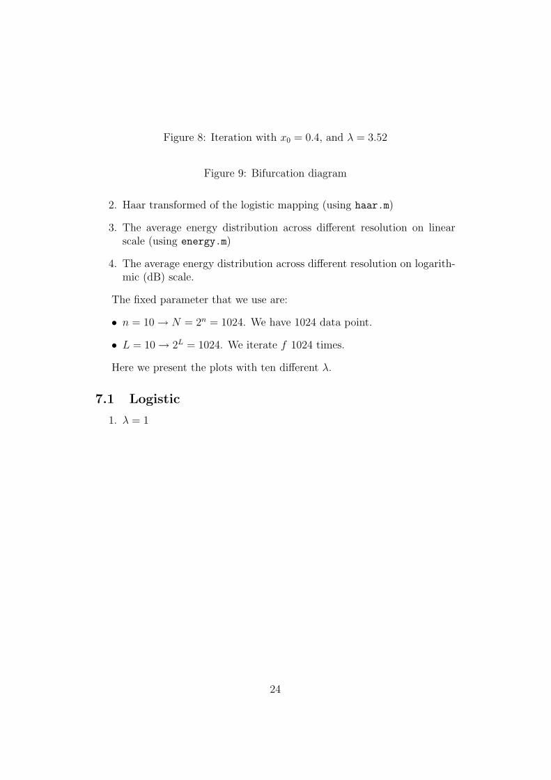
Figure 8: Iteration with x0 = 0.4, and λ = 3.52
Figure 9: Bifurcation diagram
2. Haar transformed of the logistic mapping (using haar.m)
3. The average energy distribution across different resolution on linearscale (using energy.m)
4. The average energy distribution across different resolution on logarith-mic (dB) scale.
The fixed parameter that we use are:
• n = 10→ N = 2n = 1024. We have 1024 data point.
• L = 10→ 2L = 1024. We iterate f 1024 times.
Here we present the plots with ten different λ.
7.1 Logistic
1. λ = 1
24
Figure 10: Logistic
Figure 11: Haar transformed
Figure 12: Linear scale
Figure 13: Logaritmic scale
25

2. λ = 2.8
Figure 14: Logistic
Figure 15: Haar transformed
Figure 16: Linear scale
26

Figure 17: Logaritmic scale
27

3. λ = 3.1
Figure 18: Logistic
Figure 19: Haar transformed
Figure 20: Linear scale
28
Figure 21: Logaritmic scale
29

4. λ = 3.54
Figure 22: Logistic
Figure 23: Haar transformed
Figure 24: Linear scale
30
Figure 25: Logaritmic scale
31
5. λ = 3.57
Figure 26: Logistic
Figure 27: Haar transformed
Figure 28: Linear scale
32
Figure 29: Logaritmic scale
33

6. λ = 3.575
Figure 30: Logistic
Figure 31: Haar transformed
Figure 32: Linear scale
34
Figure 33: Logaritmic scale
35

7. λ = 3.5925721
Figure 34: Logistic
Figure 35: Haar transformed
Figure 36: Linear scale
36

Figure 37: Logaritmic scale
37
8. λ = 3.6785735
Figure 38: Logistic
Figure 39: Haar transformed
Figure 40: Linear scale
38
Figure 41: Logaritmic scale
39

9. λ = 3.7
Figure 42: Logistic
Figure 43: Haar transformed
Figure 44: Linear scale
40
Figure 45: Logaritmic scale
41
10. λ = 4
Figure 46: Logistic
Figure 47: Haar transformed
Figure 48: Linear scale
42

Figure 49: Logaritmic scale
43
To proceed to a further analysis, we choose one λ (λ = 3.57) and lengthenthe number of points to 212 = 4096. Since the haar transform that we haveis combination of different scales and the average energy of coarser scale ismuch higher than finer level, we need to plot different scale separately.
7.2 Multi-Resolution
Figure 50: First scale
Figure 51: Second scale
Figure 52: Third scale
44
Figure 53: Fourth scale
Figure 54: Fifth scale
Figure 55: Sixth scale
Figure 56: Seventh scale
Figure 57: Eighth scale
Figure 58: Ninth scale
Figure 59: 10th scale
Figure 60: 11th scale
45
The best representation of these multi-resolution haar transform is bystack them one after another, and make an image representation of it. Thebrightness is related to the activity in that region (the mod square of thehaar transformed signal).
Figure 61: Image representation of multi-resolution Haar transform
The structure of the logistic map around critical lambda are interesting.But in the “sea of chaos” there are λ that give a nice structure. For examplethe “island of period three” can be found at λ = 3.835. As we can seethat the number of points is grow exponentially when we go down to thefiner scale, and as λ is bigger 3.57 we need more iteration to get a betterresolution. Therefore, to study the structure at these region, we need apowerful computer to do the computation.
At this situation quantum computer can give a better algorithm to solvethe problem. Before going any further, we will explain how quantum me-chanic do the computation.
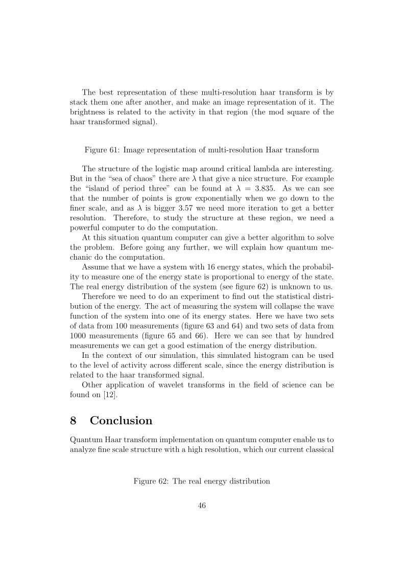
Assume that we have a system with 16 energy states, which the probabil-ity to measure one of the energy state is proportional to energy of the state.The real energy distribution of the system (see figure 62) is unknown to us.
Therefore we need to do an experiment to find out the statistical distri-bution of the energy. The act of measuring the system will collapse the wavefunction of the system into one of its energy states. Here we have two setsof data from 100 measurements (figure 63 and 64) and two sets of data from1000 measurements (figure 65 and 66). Here we can see that by hundredmeasurements we can get a good estimation of the energy distribution.
In the context of our simulation, this simulated histogram can be usedto the level of activity across different scale, since the energy distribution isrelated to the haar transformed signal.
Other application of wavelet transforms in the field of science can befound on [12].
8 Conclusion
Quantum Haar transform implementation on quantum computer enable us toanalyze fine scale structure with a high resolution, which our current classical
Figure 62: The real energy distribution
46
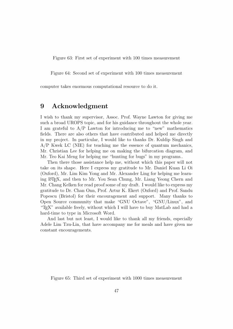
Figure 63: First set of experiment with 100 times measurement
Figure 64: Second set of experiment with 100 times measurement
computer takes enormous computational resource to do it.
9 Acknowledgment
I wish to thank my supervisor, Assoc. Prof. Wayne Lawton for giving mesuch a broad UROPS topic, and for his guidance throughout the whole year.I am grateful to A/P Lawton for introducing me to “new” mathematicsfields. There are also others that have contributed and helped me directlyin my project. In particular, I would like to thanks Dr. Kuldip Singh andA/P Kwek LC (NIE) for teaching me the essence of quantum mechanics,Mr. Christian Lee for helping me on making the bifurcation diagram, andMr. Teo Kai Meng for helping me “hunting for bugs” in my programs..
Then there those assistance help me, without which this paper will nottake on its shape. Here I express my gratitude to Mr. Daniel Kuan Li Oi(Oxford), Mr. Lim Kim Yong and Mr. Alexander Ling for helping me learn-ing LATEX, and then to Mr. You Sean Chung, Mr. Liang Yeong Chern andMr. Chang Kelken for read proof some of my draft. I would like to express mygratitude to Dr. Chan Onn, Prof. Artur K. Ekert (Oxford) and Prof. SanduPopescu (Bristol) for their encouragement and support. Many thanks toOpen Source community that make “GNU Octave”, “GNU/Linux”, and“TEX” available freely, without which I will have to buy MatLab and had ahard-time to type in Microsoft Word.
And last but not least, I would like to thank all my friends, especiallyAdele Lim Tzu-Lin, that have accompany me for meals and have given meconstant encouragements.
Figure 65: Third set of experiment with 1000 times measurement
47
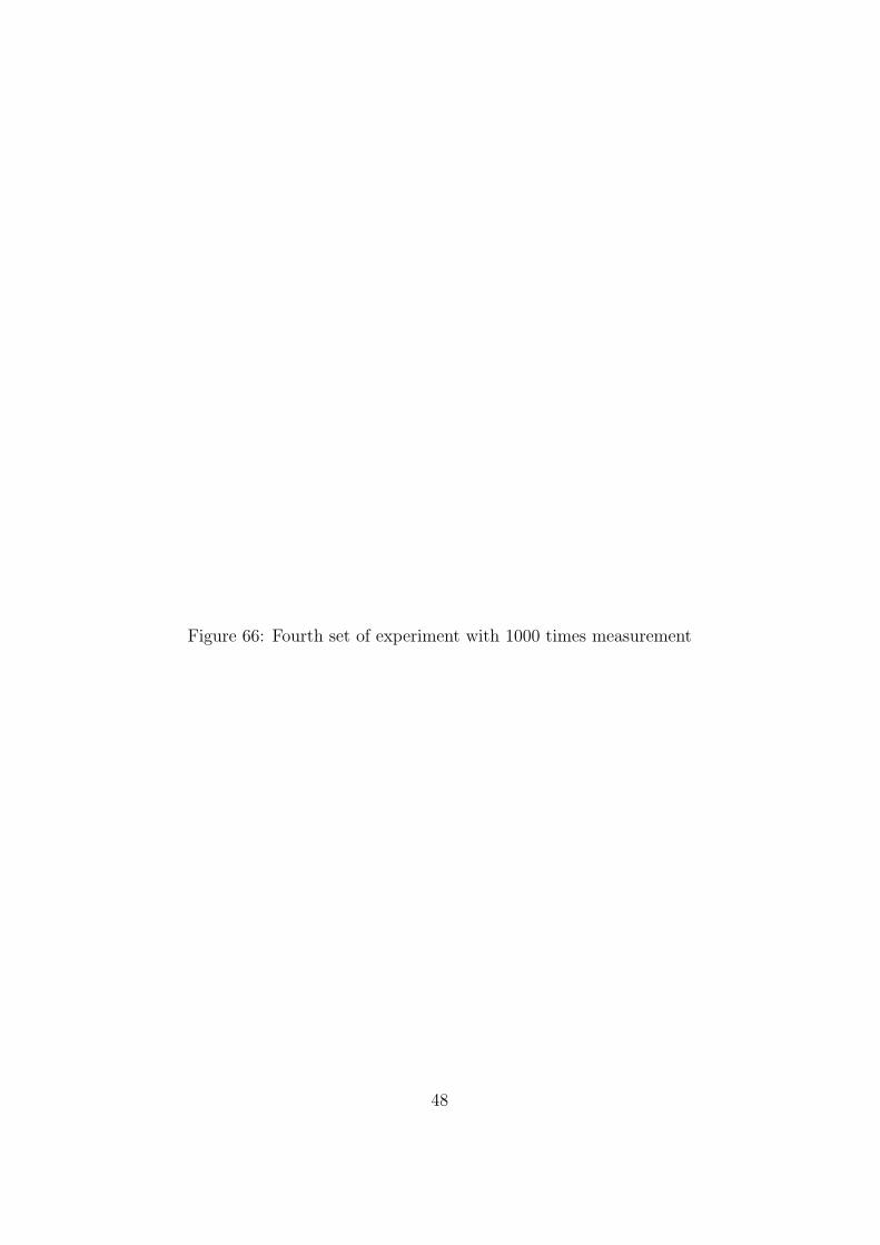
Figure 66: Fourth set of experiment with 1000 times measurement
48
Appendix
A M-files source-code:
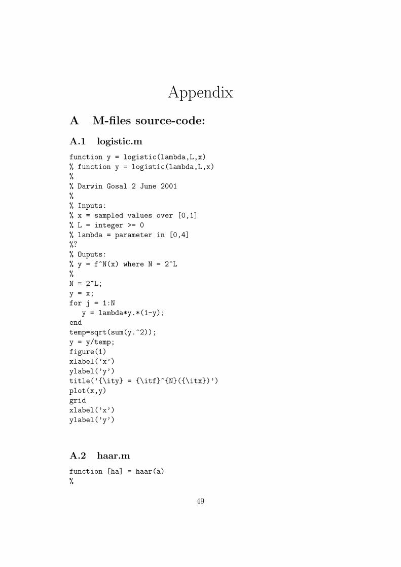
A.1 logistic.m
function y = logistic(lambda,L,x)
% function y = logistic(lambda,L,x)
%
% Darwin Gosal 2 June 2001
%
% Inputs:
% x = sampled values over [0,1]
% L = integer >= 0
% lambda = parameter in [0,4]
%?% Ouputs:
% y = f^N(x) where N = 2^L
%
N = 2^L;
y = x;
for j = 1:N
y = lambda*y.*(1-y);
end
temp=sqrt(sum(y.^2));
y = y/temp;
figure(1)
xlabel(’x’)
ylabel(’y’)
title(’{\ity} = {\itf}^{N}({\itx})’)
plot(x,y)
grid
xlabel(’x’)
ylabel(’y’)
A.2 haar.m
function [ha] = haar(a)
%
49
% function [ha] = haar(a)
%
% Darwin Gosal 7 June 2001
%
% Inputs:
% a = row array of length N=2^L
% L = integer >= 0
%
% Ouputs:
% ha = Haar transform of a
% low-frequencies/course scale on left
%
N = size(a,2);
L = log(N)/log(2);
ha = a;
for j = L:-1:1
M = 2^j;
e = ha(1:2:M);
o = ha(2:2:M);
ha(1:M) = (1/sqrt(2))*[o+e o-e];
end
A.3 haar.m
function E = energy(ha)
%
% function E = energy(ha)
%
% Darwin Gosal 8 June 2001
%
% Inputs:
% ha = the signal after Haar transform
%
% Ouputs:
% E = energy level distribution across different level
%
k = log2(max(size(ha)))-1;
for i=1:k
50
E(i)=0;
for j=2^i+1:2^(i+1)
E(i) = E(i) + ha(j)^2;
end
E(i)=E(i)/2^i;
end
Et = sum(E);
E = E/Et;
A.4 run.m
function [y, ha, E] = run(n,lambda,L)
%
% function run(n,lambda,L)
%
% Darwin Gosal 8 June 2001
%
% Inputs:
% n = the power of sample size N (N=2^n)
% L = number of iterations integer >= 0
% lambda = the variable of the logistic mapptinf
%
% Ouputs:
% It will make:
% y = which is the logistic mapping to the corresponding paramaters
% ha = which is the haar transform or y
% E = energy distribution of the mapping.
%
x = 0:1/(2^n-1):1;
y = logistic(lambda,L,x);
ha = haar(y);
figure(2);
title(’Haar transform of the signal’);
plot(5:2^n,ha(5:2^n));
E = energy(ha);
figure(3);
title(’Energy distribution on dB scale’);
plot(log10(E));
51
title(’Energy distribution on linear scale’);
figure(4);
plot(E);
A.5 mkimg.m
function img = mkimg(ha,l)
%
% function img = mkimg(ha,l)
%
% Darwin Gosal 11 June 2001
%
% Inputs:
% ha = the haar transform that going to be displayed as image
% l = number of pixels per level
%
n = log2(size(ha,2));
for i=1:n-1
c=2^(n-i-1);
for j = 2^i+1:2^(i+1)
k=j-2^i-1;
img(i,k*c+1:(k+1)*c)=ha(j);
end
end
temp=img;
for i=1:n-1
for j=l*(i-1)+1:l*i
img(j,:)=temp(i,:);
end
end
A.6 simulate.m
function B = simulate(n,s)
52
% function B = simulate(n,s);
%?% Darwin Gosal 10 June 2001
%
% Inputs:
% n = number of possible energy state
% s = number of points (degree of precision)
%
% Output:
% B = Energy distribution
A = rand(1,n);
A = A/sum(A);
A = round(A*s);
A(n)=A(n)+s-sum(A);
C = cumsum(A);A
B = ones(1,C(1));
for i=1:n-1
for m=C(i)+1:C(i+1)
B(m)=i+1;
end
end
size(B)
hist(B,n)
A.7 iteration.m
function iteration(x0,a);
% function iteration(x0,lambda);
% Darwin Gosal 12 June 2001
% x0 = starting point
% lambda = growth rate
%
X = 0:1/(2^10-1):1;
for i=1:2^10
F(i) = a*X(i)*(1-X(i));
G(i) = X(i);
end
53
clear x;
for i=0:2:100
if i==0
x(i+1)=x0;
y(i+1)=a*x(i+1)*(1-x(i+1));
x(i+2)=y(i+1);
y(i+2)=y(i+1);
else
x(i+1)=y(i-1);
y(i+1)=a*x(i+1)*(1-x(i+1));
x(i+2)=y(i+1);
y(i+2)=y(i+1);
endif
end
plot(x,y)
hold
plot(X’,F)
plot(X’,G)
A.8 fwt.m
function h = fwt(m,l)
% function h = fwt(m,l)
%
% Dariwn Gosal, June 6, 2001
%
% Inputs:
% m = input size
% l = level
%
% Output:
% h = l level haar decomposition
if(nargin != 2)
54
error("fwt:invalid number of arguments");
endif
n=log2(m);
if(l > n)
error("fwt: 2nd parameter must be less the the log2 of the first parameter");
endif
h=eye(m);
for i=1:l
B=[1 1];
C=[1 -1];
D=[]; E=[];
k=m/2^i;
for j=1:k
D=blkdiag(D,B);
E=blkdiag(E,C);
end
F=(1/sqrt(2))*[D zeros(k,m-2*k); E zeros(k,m-2*k);
zeros(m-2*k,2*k) eye(m-2*k)];
h = F*h;
end
55
References
[1] Andreas Klappenecker, Wavelets and Wavelet Packets on QuantumComputers. quant-ph/9909014
[2] Amir Fijany and Colin P. Williams, Quantum Wavelet Transforms: FastAlgorithms and Complete Circuits. quant-ph/9809004
[3] Michael A. Nielsen and Isaac L. Chuang, Quantum computation andquantum information. Cambridge University Press, 2000.
[4] Arthur O. Pittenger, An introduction to quantum computing algo-rithms. Birkhauser, 2000.
[5] Dirk Bouwmeester, Artur K. Ekert, and Anton Zeilinger, The physics ofquantum information : quantum cryptography, quantum teleportation,quantum computation. New York, Springer, 2000.
[6] Jozef Gruska, Quantum computing. London, McGraw-Hill, 1999.
[7] Gennady P. Berman (et al.), Introduction to quantum computers. WorldScientific, 1998.
[8] Chris J. Isham, Lectures on quantum theory : mathematical and struc-tural foundations. Imperial College Press, London, 1995.
[9] John von Neumann, Mathematical Foundations of Quantum Mechanics.Princeton University Press, 1983.
[10] Macchiavello C., Palma G.M., Zeilinger A., Quantum Computation andQuantum Information Theory. World Scientific, 2000.
[11] Cabello A., Bibliographic guide to the foundations of quantum mechan-ics and quantum information. quant-ph/0012089
[12] Dremin I.M., Ivanov O.V., Nechitailo V.A., Wavelets and Their Use.hep-ph/0101182
[13] Richard Jozsa, Quantum Algorithms and the Fourier Transform. quant-ph/9707033
[14] John Preskill, The Future of Quantum Information Science. A talk atthe NSF Workshop on Quantum Information Science, 28 October 1999.
[15] Ekert A., Hayden P., and Inamori H., Basic Concepts in Quantum Com-putation. quant-ph/0011013
56
[16] Gilbert Strang and Truong Nguyen, Wavelets and Filter Banks.Wellesley-Cambridge Press, 1996.
[17] Burrus C.S., Gopinath R.A., Guo H., Introduction to Wavelets andWavelet Transforms: A Primer. Prentice-Hall, 1998.
[18] Charles K. Chui, An Introduction to Wavelets. Academic Press, 1992.
[19] Chan A.K. and Liu S.J., Wavelet Toolware: Software for Wavelet Train-ing. Academic Press, 1998.
57