arX

iv:2

109.

0844

0v1

[he

p-ph

] 1

7 Se

p 20

21

Quantum Kinetic Theory with Vector and Axial Gauge Fields

Zhou Chen∗ and Shu Lin†

School of Physics and Astronomy, Sun Yat-Sen University, Zhuhai 519082, China

(Dated: September 20, 2021)

Abstract

In this paper we introduce the axial gauge field to the framework of the quantum kinetic theory

with vector gauge field in the massless limit. Treating axial-gauge field on an equal footing with the

vector-gauge field, we construct a consistent solution to the kinetic equations up to the first order in

gradient expansion or equivalently the semi-classical expansion. The intuitive extension of quantum

kinetic theory presented in this work provides a natural generalization, and turns out to give rise

to the covariant anomaly and the covariant currents. The corresponding consistent currents can

be obtained from the covariant ones by adding the Chern-Simons current. We use the consistent

currents to calculate various correlation functions among currents and energy-momentum tensor

in equilibrium state.

∗ chenzh339@mail2.sysu.edu.cn† linshu8@mail.sysu.edu.cn

1

I. INTRODUCTION

The quantum kinetic theories for spinning particles has received much attention over

the past few years. The most prominent one is quantum kinetic theory for spin one half

particle, which has been widely used in the studies of spin sensitive transports. Its massless

limit, chiral kinetic theory(CKT) [1–18], has provided a novel description of the celebrated

chiral magnetic effect [19–21] and chiral vortical effect [22–25]. More recently, generalization

to the massive case, axial kinetic theory(AKT) [26–30], has revealed additional degrees of

freedom not present in the CKT. The inclusion of mass is a crucial step towards realistic

description of particle polarization. The axial kinetic theory has been applied to physics of

spin polarization in heavy ion collisions, see [31] for a review. Collisional effects have been

studied in [5, 32–44]. Quantum kinetic theory for particles with other spins have been also

constructed [45–47].

The quantum kinetic theory also offers a way to derive hydrodynamics from a microscopic

theory. A key element of hydrodynamics is the response of spin one half particles to external

sources, including vector gauge field and torsionful metric. These allow for derivation of

anomalous hydrodynamics [15, 48–51], magnetohydrodynamics [17] and spin hydrodynamics

[37, 52–54][55]. In fact, a more complete anomalous hydrodynamics also include response to

axial gauge field [24, 56]. It is desirable to extend the present framework of quantum kinetic

theory to incorporate axial gauge field as well. The purpose of introducing axial gauge

field is twofold. On one hand, while axial gauge field is not a physical gauge field, it can be

mimicked in system like Weyl semi-metal leading to physical effects [57]. On the other hand,

the axial gauge field can also serve as a convenient tool for deriving correlation functions of

axial current. In the same spirit, vierbein and spin connection in torsionful metric allows for

derivation of correlation functions of energy-momentum tensor and spin tensor [58]. Since

spin tensor and axial current are related, our approach can be an alternative to theory with

torsionful metric.

As is well known, introducing the axial gauge field leads to ambiguity in the definition

of current: consistent current versus covariant current, see [59] for a review. The purpose

of this study is to integrate axial field in the framework of quantum kinetic theory. As

we shall see, it is convenient to treat vector/axial gauge fields on the equal footing. This

corresponds to working with covariant current. The derivation of correlation functions uses

2

consistent current instead. We will illustrate how to calculate correlation functions with

simple examples.

This paper is structured as follows: in Section II, we derive chiral kinetic theory with

vector/axial gauge field in the collisionless limit; in Section III, we present solution of the

kinetic equation up to first order in gradient; Section IV is devoted to the calculation of

one-point functions, which give rise to anomalous transports and multi-point correlation

functions. We summarize and provide an outlook in Section V. Detail of calculations is left

to two appendices.

II. QUANTUM KINETIC EQUATIONSWITH VECTOR/AXIAL GAUGE FIELDS

With both the vector and axial gauge fields, the chiral fermion Lagrangian with the gauge

fields as backgrounds is given by

L = iψ /Dψ. (1)

Dµ = ∂µ+iAµ+iγ5A5

µ is the extended covariant derivative, with Aµ and A5µ being the vector

and axial gauge potential, respectively. And the coupling constants have been absorbed

into the corresponding gauge potentials. In the current work, we restrict ourselves to the

collisionless limit. The kinetic equation is formulated in terms of the Wigner function defined

as

S<

αβ(x, y) = 〈ψβ(y)ψα(x)〉,

S<αβ(p,X) =

∫

d4seip·sS<

αβ(x, y), (2)

with X = x+y

2and s = x− y. S

<

αβ(x, y) satisfies the Dirac equation

DxS<

αβ(x, y) = 0. (3)

Assuming constant field strength for the vector and axial fields, we can Fourier transform

Eq.(3) to obtain the EOM of S<αβ(p,X)

γµ

(

Kµ +i

2Dµ + γ5Πµ

)

S<(p,X) = 0, (4)

where Kµ = pµ −Aµ, Dµ = ∂X,µ + (∂X,νAµ)∂νp and Πµ = A5

µ +i2(∂X,νA

5µ)∂

νp . Dµ and Πµ are

organized as a gradient expansion in ∂X [60], with Aµ, A5µ ∼ O(∂0X). To avoid the subtleties of

3

the axial-gauge symmetry, we proceed by solving Eq.(4) directly without defining any gauge

link. It turns out that the gauge-linked Wigner function can be obtained from the bare

one by replacing the canonical momentum pµ by the kinetic momentum kµ = pµ −Aµ ∓A5µ

corresponding to right and left-handed components respectively. It follows that the resulting

solution is invariant under both vector and axial gauge symmetry, leading to covariant vector

and axial currents.

TheWigner function S<(p,X), satisfying the “hermitian” condition S<(p,X) = γ0S<(p,X)†γ0,

can be decomposed in terms of 16 independent generators of the Clifford algebra,

S<(p,X) =1

4

[

F + iγ5P + γµVµ + γ5γµAµ +σµν

2Sµν

]

, (5)

with the real coefficients F , P, Vµ, Aµ and Sµν being its scalar, pseudo-scalar, vector,

axial-vector and tensor components respectively. To lighten the notation, the phase-space

coordinates (p,X) of the Clifford-algebra coefficients have been omitted. We can further

derive

γµS<(p,X) =1

4

[

Vµ − γ5Aµ + γν (gµνF + iSµν)

+γ5γν

(

Sµν − igµνP)

−σαβ2

(

ǫµναβAν + i(

gµαVβ − gµβVα))

]

,(6)

γ5γµS<(p,X) =1

4

[

−Aµ + γ5Vµ + γν

(

Sµν − igµνP)

+γ5γν (gµνF + iSµν) +

σαβ2

(

ǫµναβVν + i(

gµαAβ − gµβAα))

]

,(7)

where we have used the dual tensor Sµν = 12ǫµνρσSρσ and the following identities:

γµγαγβ = gµαγβ − gµβγα + gαβγµ − iǫµαβλγ5γλ, γ5σµν =i

2ǫµνκλσ

κλ. (8)

Inserting Eqs.(6) and (7) into Eq.(4), and comparing the real and imaginary parts of the

coefficients in the Clifford-algebra basis, we will obtain two sets of equations. We see that

the equations for Aµ and Vµ are decoupled from other components,

KµVµ −A5

µAµ = 0,

DµAµ + (∂X,λA

5µ)∂

λpV

µ = 0,

KµAν −KνAµ − A5µVν + A5

νVµ +1

2ǫµναβD

αVβ +1

2ǫµναβ(∂λA

α5 )∂

λpA

β = 0,

(9)

KµAµ − A5

µVµ = 0,

DµVµ + (∂X,λA

5µ)∂

λpA

µ = 0,

KµVν −KνVµ − A5µAν + A5

νAµ +1

2ǫµναβD

αAβ +1

2ǫµναβ(∂λA

α5 )∂

λpV

β = 0.

(10)

4

The equations can be further decoupled in the chiral basis

ksµJµs = 0, (11)

∇sµJ

µs = 0, (12)

kµsJνs − kνsJ

µs +

s

2ǫµναβ∇s

αJsβ = 0, (13)

where the chiral components J µs of the Wigner function are defined as

J µs =

1

2(Vµ + sAµ) , (14)

with s = + and s = − for right-handed and left-handed fermions respectively. ksµ = pµ−Asµ

is the kinetic momentum with the gauge potential in the chiral basis being Asµ = Aµ + sA5

µ.

∇sµ = ∂µ + (∂νA

sµ)∂

νp is the covariant derivative at O(∂X). Note that the kinetic momenta

and covariant derivatives differ for the right and left handed components in the presence of

axial gauge field.

III. SOLUTION TO THE KINETIC EQUATIONS

We solve Jµ by gradient expansion up to first order,

J sµ = J s(0)

µ + J s(1)µ + · · · , (15)

where the superscripts (0), (1), · · · denotes the orders in the expansion. Substituting this

expansion into Eqs.(11)-(13) and requiring that the equations hold order by order, the

equations for Js(n)µ with n = 1 and n = 0 read

ksµJs(n)µ = 0, (16)

∇sµJ

s(n)µ = 0, (17)

ksµJs(n)ν − ksνJ

s(n)µ +

s

2ǫµναβ∇

αsJ

s(n−1)β = 0, (18)

where we have defined Js(−1)µ = 0. Contracting both sides of Eq.(18) with kµs and using

Eq.(16), we have

k2sJs(n)µ =

s

2ǫµναβk

νs∇

αsJ

s(n)β. (19)

5

The solution of Eq.(19) implies a general form of Js(n)µ :

J s(n)µ = Js(n)

µ δ(k2s) +s

2k2sǫµναβk

νs∇

αsJ

s(n−1)β , (20)

where Js(n)µ is nonsingular at k2s = 0, and can be constrained by substituting Eq.(20) back into

Eq.(18). From Eq.(16), we can also obtain a further constraint for Js(n)µ : kµs J

s(n)µ δ(k2s) = 0.

When n = 0, the equation of motion depend on kinetic momentum only. It is straight-

forward to write down the solution,

J s(0)µ = ksµδ(k

2s)fs(ks, X). (21)

To be specific, in this paper we choose the zeroth order distribution function to be Fermi-

Dirac distribution in kinetic momentum

fs(ks, X) =2

(2π)3[θ(u · ks)fFD(β · ks − µs) + θ(−u · ks)fFD(−β · ks + µs)] , (22)

where the Fermi-Dirac distribution function fFD(z) ≡ [exp(z) + 1]−1, βµ ≡ βuµ with β =

βµuµ ≡ 1/T being the inverse temperature and uµ being the fluid velocity, and µs = βµs

with µs = µ + sµ5 being the chemical potential for chirality s = ±1. The hydrodynamic

quantities βµ, β and µs can be dependent on X .

Using the definitions of ksµ and ∇sµ given in Sec.II, we can derive the following useful

identities,

∇sµk

sν = −F s

µν ,

∇sµδ

(n)(k2s) = −2F sµνk

νs δ

(n+1)(k2s),(23)

where we have defined F sµν ≡ ∂µA

sν − ∂νA

sµ = Fµν + sF 5

µν and δ(n)(k2) =(

ddk2

)nδ(k2).

Especially, it follows that ∇sµ [k

µs δ(k

2s)] = 0. Using this identity, it is easy to show that

∇sµJ

(0)µs = ∇µ

[

kµs δ(k2s)fs(X, ks)

]

= δ(k2s)kµs∇µfs(X, ks).

(24)

It implies the constraint equation kµs∇s,µfs = 0 in order for Eq.(17) to hold. With the

distribution function given by Eq.(22), we can evaluate kµs∇s,µfs = 0 as

kµs∇sµfs =

∂fs∂(β · ks)

kµs[

∇µ(β · ks)−∇sµµs

]

=∂fs

∂(β · ks)kµs

[

kνs∂µβν − ∂µµs − F sµνβ

ν]

.

(25)

6

Accordingly we deduce the conditions for the chiral systems to be in global equilibrium, that

is

∂µβν + ∂νβµ = 0, (26)

∂µµs = −F sµνβ

ν . (27)

Eq.(26) is the Killing condition for βµ which leads to the solution βµ = bµ − Ωµνxν with

bµ and the thermal vorticity Ωµν = 12(∂µβν − ∂νβµ) being constants. Eq.(27) takes a more

familiar form in the original basis. With µ = 12(µ+ + µ−) and µ5 =

12(µ+ − µ−), we have

∂µµ = −Fµνβν , (28)

∂µµ5 = −F 5µνβ

ν . (29)

Eq.(28) implies the electric field is balanced by gradient of chemical potential. Eq.(29) is

just the axial counterpart of Eq.(28).

With the help of the conditions given by Eqs.(26) and (27), we can derive that

∇µfs = f ′sΩµνk

νs , (30)

where f ′s ≡

∂fs∂(β·ks)

. Substituting the zeroth order solution Eq.(21) into Eq.(20) gives the first

order solution (n = 1):

J s(1)µ = Js(1)

µ δ(k2s) +s

2k2sǫµναβk

νs∇

αsJ

s(0)β

= Js(1)µ δ(k2s) + sF s

µνkνsfsδ

′(k2s),

(31)

where we have used F sµν = 1

2ǫµναβF

αβs and δ′(k2s) = −δ(k2s)/k

2s . Then, substituting Eqs.(21)

and (31) into Eq.(18), we arrive at

ksµ

(

Js(1)ν δ(k2s) + sF s

νρkρsfsδ

′(k2s))

− [µ ↔ ν] = −s

2ǫµναρ∇

αs

[

kρsfsδ(k2s)]

. (32)

It help us to determine Js(1)µ = − s

2Ωµνk

νsf

′s. Details of the determination are presented in

Appendix A. We summarize the solution of the Wigner function up to the first order:

J sµ = kµs δ(k

2s)fs −

s

2Ωµνk

νs δ(k

2s)f

′s + sF s

µνkνs δ

′(k2s)fs. (33)

Eq.(33) generalizes the known solution to the case with axial gauge fields [15]. In fact,

we can show they are equivalent upon proper identification. In the absence of axial gauge

field, the vector gauge link is inserted as

S<

link(x, y) = S<(x, y)e−i

∫x

ydz·A(z) = S

<(x, y)e−is·A(X) +O(∂2X). (34)

7

We have used the subscript link to indicate that the corresponding quantities have explicit

gauge link insertion. The vector gauge invariant S<

link(x, y) is then Wigner transformed with

kinetic momentum:

S<link(k,X) =

∫

d4seik·sS<

link(x, y), (35)

generating the gauge invariant observables from components of Wigner function. Impor-

tantly the momentum appearing in Eq.(35) should be the gauge invariant kinetic momentum

k. We choose to work with bare Wigner function, which is then transformed with canonical

momentum p. From Eq.(34), we can easily obtain

eik·sS<

link(x, y) = eip·sS<(x, y)

⇒ S<link(k,X) = S<(p,X). (36)

It shows that up to O(∂X), our bare Wigner function is also vector gauge invariant: the

gauge dependence in our bare Wigner function is canceled by the gauge dependence in the

canonical momentum in the Wigner transform. Therefore components of our S<(p,X) is

also gauge invariant, whose momentum integration give rise to physical observables. When

the axial gauge field is present, it is straightforward to deduce S<(p,X) is invariant under

both vector and axial gauges. In fact, we may equivalently working with Wigner functions

for right and left-handed fermions with appropriate gauge link insertion:

Ss(x, y) = 〈ψs(x)ψ†s(y)〉,

Ss,link(x, y) = Si(x, y)e−i∫x

ydz·As(z), (37)

with ψ+ ≡ ψR and ψ− ≡ ψL standing for right and left handed fermions respectively.

IV. ANOMALOUS TRANSPORTS AND CORRELATION FUNCTIONS

Integrating Eq.(33) over the kinetic momentum ks, we obtain the left-handed and right-

handed currents jµs (X) up to the first order in ∂X

jµs (X) =

∫

d4ksJµs (ks, X), (38)

Both the solution Eq.(33) and integration measure are vector/axial gauge invariant, it follows

that the resulting currents are gauge invariant.

8

After the four-momentum integrations, we have the zeroth order contribution given by

J(0)µs , and the first order contribution given by J

(1)µs :

j(0)µs = nsuµ, (39)

j(1)µs = ξsωµ + ξBsB

µs , (40)

with ns being the fermion number density, ξs and ξBs related to transport coefficients of chiral

vortical effect (CVE), chiral magnetic effect (CME) and chiral separation effect (CSE). The

vorticity and magnetic field are defined as ωµ = T Ωµνuν and Bµs = F µν

s uν respectively

according to the decomposition,

F sµν = Bs

µuν − Bsνuµ − ǫµναβu

αEβs , F s

µν = Esµuν −Es

νuµ + ǫµναβuαBβ

s , (41)

T Ωµν = ωµuν − ωνuµ − ǫµναβuαεβ, TΩµν = εµuν − ενuµ + ǫµναβu

aωβ. (42)

And the coefficients ns, ξs and ξBs are given by

ns =µs

6π2

(

π2

β2+ µ2

s

)

, (43)

ξs =s

12π2

(

π2

β2+ 3µ2

s

)

. (44)

ξBs =s

4π2µs (45)

The vector and axial currents can be obtained from the linear combinations of jµ±:

jµ = jµ+ + jµ−, jµ5 = jµ+ − jµ−. (46)

Then the zeroth order vector and axial currents read

j(0)µ = nuµ, (47)

j(0)µ5 = n5u

µ. (48)

From the first order currents, we can obtain the vector and axial currents in the CVE

jµω = ξωµ, (49)

jµ5,ω = ξ5ωµ, (50)

while the vector and axial currents in the CME are

jµB = ξBBµ + ξB5B

µ5 , (51)

9

jµ5,B = ξB5Bµ + ξBB

µ5 , (52)

where

n =µ

3π2

(

π2

β2+ µ2 + 3µ2

5

)

, n5 =µ5

3π2

(

π2

β2+ 3µ2 + µ2

5

)

,

ξ =µµ5

π2, ξ5 =

1

6β2+

µ2

2π2+

µ25

2π2, ξB =

µ5

2π2, ξB5 =

µ

2π2.

(53)

The gauge invariant canonical energy-momentum tensor can be obtained by

T µν =

∫

d4k+Jµ+(k+, X)kν+ +

∫

d4k−Jµ−(k−, X)kν−

≡ T µν+ + T µν

− .

(54)

Then we can perform the four momentum integrals to obtain

T (0)µνs =

(

uµuν −1

3∆µν

)

ρs, (55)

T (1)µνs = sns(u

µων+uνωµ)+ξs2(uµBν

s +uνBµ

s − ǫµναβuαE

sβ)−

sns

2(uµων −uνωµ+ ǫµναβuαεβ),

(56)

with

ρs =7

120

π2

β4+

1

4

µ2s

β2+

1

8π2µ4s. (57)

Eqs.(56) and (57) generalize the first order results in [15] to the case with axial gauge field.

We can further separate the symmetric and anti-symmetric parts of the canonical energy-

momentum tensor as[61]

T (0)µν =

(

uµuν −1

3∆µν

)

ρ, (58)

T (1)µν = n5(uµων + uνωµ) +

ξ

2(uµBν + uνBµ) +

ξ52(uµBν

5 + uνBµ5 ), (59)

T (1)[µν] = −ξ

2ǫµναβuαEβ −

ξ52ǫµναβuαE

5β −

n5

2(uµων − uνωµ + ǫµναβuαεβ), (60)

where T µν ≡ Tµν+T νµ

2and T [µν] ≡ Tµν−T νµ

2. ρ = 7

60π2

β4 + 12

µ2+µ2

5

β2 + 14π2 (µ

4 + 6µ2µ25 + µ4

5) is

the energy density. The RHS of Eq.(59) corresponds to heat flow along vorticity, magnetic

and axial magnetic fields respectively. The first two need chiral imbalance in the fluid to

exist while the last one exists even in the neutral medium. As we shall see shortly, the

10

last one can be related to axial chiral vortical effect by Onsager relation. Using the Killing

conditions, we show in Appendix B the following conservation equations

∂µjµ =

1

2π2

(

~E5 · ~B + ~E · ~B5

)

, (61)

∂µjµ5 =

1

2π2

(

~E · ~B + ~E5 · ~B5

)

, (62)

∂µTµν = F νµjµ + F µν

5 j5,µ, (63)

∂µT[µν] = 0, (64)

T [µν] = ∂λSλµν . (65)

Eqs.(61) and (62) are current conservation equations. Eqs.(63) and (64) are the energy-

momentum conservation subject to external force by vector and axial gauge fields. Eq.(65)

corresponds to change rate of spin tensor Sλµν .

We will be mainly interested in correlation functions among vector/axial currents, which

are obtainable by functional derivatives with respect to vector/axial gauge potential. For

this purpose, we may turn off the vorticity and set uµ = (1, 0, 0, 0). The Killing condition

∂µβν + ∂νβµ = 0 implies a homogeneous temperature.

It is known that the definition of current is not unique when axial gauge field is present.

One can choose either consistent current and covariant current [59], with the former always

conserve vector current and the latter is symmetric with respect to the interchange of vec-

tor/axial components. The construction of our solution suggests the corresponding current

to be covariant current. Indeed, the anomaly equations we obtained Eqs.(61) and (62) agree

with those of covariant current.

Now we turn to the calculation of correlation functions. A convenient way to calcu-

late correlation function is to take functional derivatives with respect to vector/axial gauge

potential. Note that each functional derivative brings down a consistent current as

δ

δAµ(x)eiΓ[A,A5] = jµcons(x)e

iΓ[A,A5],δ

δA5µ(x)

eiΓ[A,A5] = jµ5,cons(x)eiΓ[A,A5], (66)

with Γ[A,A5] being the effective action. Taking multiple derivatives give multi-point corre-

lation functions. We illustrate this with examples of two and three point functions. Instead

of finding the effective action, we start with one-point function of consistent currents, which

11

are related to the covariant currents in Eqs.(51) and (52) by [59]

jµcov = jµcons +1

4π2ǫµνρσA5,νFρσ,

jµ5,cov = jµ5,cons +1

12π2ǫµνρσA5,νF5ρσ. (67)

From Eqs.(51) and (52), we obtain

jicons =1

2π2(µ5 − A5

0)Bi +1

2π2µBi

5,

ji5cons =1

2π2(µ5 −

A50

3)B5

i +1

2π2µBi. (68)

Possible contribution from vector/axial electric fields are not included in Eq.(68) for the

following reason: they need to be balanced by gradients of corresponding chemical potentials.

Since we will calculate correlation functions in system with constant chemical potential and

temperature, we simply turn them off. We will calculate correlation functions for equilibrium

state without axial gauge field, i.e. A5,µ = 0. Eq.(68) indicates the only nonvanishing

correlation functions are two-point and three-point ones. The former comes from CME and

CSE terms (and their analogs with axial magnetic field). Fourier transforms of these terms

give

jicons(k) =1

2π2µ5Bi(k) +

1

2π2µBi

5(k),

ji5,cons(k) =1

2π2µ5B

5i (k) +

1

2π2µBi(k), (69)

where we use tilde to indicate operators in Fourier space. The absence of electric fields re-

quires momenta appearing in the Fourier transforms contain no temporal components. Tak-

ing functional derivative once, and noting the coupling∫

d4xAµ(x)jµcons(x) =

∫

d4k(2π)4

Aµ(k)jµcons(−k)

and similarly for axial counterpart, we obtain

〈jicons(k)jjcons(−k)〉 =

iµ5ǫijkkk

2π2,

〈jicons(k)jj5,cons(−k)〉 =

iµǫijkkk

2π2,

〈ji5,cons(k)jj5,cons(−k)〉 =

iµ5ǫijkkk

2π2,

〈ji5,cons(k)jjcons(−k)〉 =

iµǫijkkk

2π2, (70)

where the LHS are defined by 〈X(k)Y (p)〉 = 〈X(k)Y (−k)〉(2π)4δ(4)(k + p). The terms

quadratic in A(A5) give rise to the three-point correlation functions. Fourier transforms of

12

these terms are given by

jicons(q) =

∫

d4k

(2π)4[

−1

2π2A5

0(q − k)Bi(k)]

,

ji5,cons(q) =

∫

d4k

(2π)4[

−1

6π2A5

0(q − k)B5i (k)

]

. (71)

Taking functional derivatives twice, we obtain the following three-point correlation functions

〈jicons(q)j05,cons(k − q)jjcons(−k)〉 = −iǫijk

kk

2π2,

〈ji5,cons(q)j05,cons(k − q)jj5,cons(−k)〉 = −iǫijk

kk

6π2, (72)

where the LHS are defined by 〈X(k)Y (q)Z(p)〉 = 〈X(k)Y (q)Z(−k− q)〉(2π)4δ(4)(k+ q+ p).

In the limit q → k, Eq.(72) are in agreement with the results obtained with field theory and

holography [25].

We can also calculate correlation functions between energy-momentum tensor and cur-

rents. From Eq.(59) and the fact Eµ = E5,µ = 0, it is clear the nonvanishing correlation

functions involves only symmetric part of the energy-momentum tensor:

〈T 0i(k)jjcons(−k)〉 =ξ

2ǫijkikk,

〈T 0i(k)jj5,cons(−k)〉 =ξ52ǫijkikk, (73)

Indeed, they can be related to CVE in Eq.(50). Noting that ω can be induced by metric

perturbation as

ωj = −1

2ǫijk∂kh0i, (74)

we find from Eqs.(49) and (50)

〈jjcons(k)T0i(−k)〉 =

ξ

2ǫijkikk,

〈jj5,cons(k)T0i(−k)〉 =

ξ52ǫijkikk. (75)

Eq.(75) and Eq.(73) are consistent with Onsager relation[62].

V. SUMMARY AND OUTLOOK

We have derived chiral kinetic theory with both vector and axial gauge fields. We have

also found a solution preserving both vector and axial gauge symmetry, leading to covariant

13

vector and axial currents. The introduction of axial gauge field allows us to derive correlation

functions of vector/axial current. This is done by first converting covariant currents to

consistent current and then taking functional derivatives with respect to vector/axial gauge

fields. We find the resulting correlation functions in agreement with known field theoretic

results.

The present work can be extended in two aspects. Firstly, mass effect can be included.

Since mass breaks axial symmetry explicitly, it requires non-trivial modification to the solu-

tion presented in this work. It is known that mass introduces additional degrees of freedoms.

It would be interesting to see how the dynamics of these degrees of freedoms are affected by

the presence of axial gauge field. More interestingly, collisional effect should be included for

a complete description of dynamics, in particular for axial current (or spin density). This

would provide a route to spin hydrodynamics for weakly interacting fermion system.

Appendix A: Verification of Eqs.(17) and determination of Js(1)µ

We determine Js(1)µ from Eq.(32):

(

ksµJs(1)ν − ksνJ

s(1)µ

)

δ(k2s) = −s(

ksµFsνρ − ksνF

sµρ

)

kρsfsδ′(k2s)−

s

2ǫµναρ∇

αs

[

kρsfsδ(k2s)]

= −s(

ksµFsνρ − ksνF

sµρ + ksρF

sµν

)

kρsfsδ′(k2s) +

s

2ǫµνραk

ρs∇

αs

[

fsδ(k2s)]

= sǫµνραFαβs ksβk

ρsfsδ

′(k2s) +s

2ǫµνραk

ρs∇

αs

[

fsδ(k2s)]

=s

2ǫµνραk

ρsΩ

αβksβf′sδ(k

2s),

(A1)

where we have used Eqs.(23,30), and the Schouten identity

gρσǫµναβ + gβσǫ

ρµνα + gασǫβρµν + gνσǫ

αβρµ + gµσǫναβρ = 0, (A2)

from which we can show that kµs Fνρs + kρs F

µνs + kνs F

ρµs + ǫµνραF s

αβkβs = 0 by contracting both

sides with F sαβkσ and using the antisymmetric nature of the field strength tensors. At this

stage, we can express the tensor in terms of the dual tensor: Ωαβ = −12ǫαβκλΩκλ. And the

Levi-Civita tensors can be contracted as

ǫµνρσǫµναβ = −2! δρσαβ = −2(δραδσβ − δρβδ

σα),

ǫµκρσǫµναβ = −δκρσναβ = −δκν (δραδ

σβ − δρβδ

σα)− δκα(δ

ρβδ

σν − δρνδ

σβ )− δκβ(δ

ρνδ

σα − δραδ

σν ).

(A3)

14

Using these contract relations, we can further derive for two arbitrary antisymmetric tensors,

e.g. Ωµν and F sµν , that

1

2ΩµνF s

µνk2s = ΩµαF s

µρksαk

ρs + ΩµαF s

µρksαk

ρs , (A4)

and especially,

ΩµνΩµνk2s = 4ΩµαΩµρk

sαk

ρs ,

F µνs F s

µνk2s = 4F µα

s F sµρk

sαk

ρs .

(A5)

Then Eq.(A1) can be written as

(

ksµJ(1)ν − ksνJ

(1)µ

)

δ(k2s) =s

2ǫµνραk

ρsΩ

αβksβf′Sδ(k

2s)

= −s

4ǫµνραǫ

αβκλΩκλkρsk

sβf

′sδ(k

2s)

= −s

4δβκλµνρ k

ρs Ωκλk

sβf

′sδ(k

2s)

= −s

2

(

ksµΩνρkρs − ksνΩµρk

ρs

)

f ′δ(k2s).

(A6)

We have thrown away the terms proportional to k2sδ(k2s) = 0. In fact, Eq.(A6) cannot exclude

the correction of the form δJ(1)µ = ksµX

(1), which involves an unknown regular function X(1)

that should be identified as of the first order in gradient. We may absorb this undetermined

correction into the first order distribution function which we do not consider in this work.

After that, we can set Js(1)µ = − s

2Ωµνk

νsf

′s in line with Eq.(A6).

Now we check if the first-order solution given by Eq.(33) satisfies Eq.(17) with the global

equilibrium conditions which have been embedded into Eq.(30). For convenience, we divide

the Wigner function into two parts, Js(1)µΩ and J

s(1)µEM , which are generated by vorticity and

background fields respectively. We note that the vorticity Ωµν is constant due to the Killing

condition ∂µβν + ∂νβµ = 0. Assuming the constant field strength tensors, i.e. ∂ρFsµν = 0, we

can show that

∇sµJ

s(1)µΩ = −

s

2Ωµν∇s

µ

[

ksνf′sδ(k

2s)]

=s

2ΩµνF s

µνf′sδ(k

2s) + sΩµνF s

µρksνk

ρsf

′sδ

′(k2s)−s

2ΩµνΩµρk

sνk

ρsf

′′s δ(k

2s)

= −sΩµν F sµρk

sνk

ρsf

′sδ

′(k2s),

(A7)

and

∇sµJ

s(1)µEM = sF µν

s ∇sµ

[

ksνfsδ′(k2s)

]

= −sF µνs F s

µνfsδ′(k2s)− 2sF µν

s F sµρk

sνk

ρsfsδ

′′(k2s) + sF µνs Ωµρk

sνk

ρsf

′sδ

′(k2s)

= sF µνs Ωµρk

sνk

ρsf

′sδ

′(k2s).

(A8)

15

where we have used δ′(k2) = −δ(k2)/k2, δ′′(k2) = −2δ′(k2)/k2 and Eq.(A5). By taking the

sum of Eq.(A7) and Eq.(A8), we obtain

∇µJ(1)µ = 0. (A9)

Appendix B: Conservation equations

Using Eqs.(26) and (42) with the definition βµ ≡ βuµ = uµ/T , we can easily show that

∂µβµ ≡ ∂µ

uµ

T= 0, (B1)

∂µβ = uν∂µβν − βuν∂µuν = uνΩµν = βεµ. (B2)

u · ∂β = 0, ∂µuµ = 0 (B3)

∂µuν = TΩµν − εµuν (B4)

And we have used u · ε = 0, u2 = 1 and uν∂µuν = 0. Then from Eqs.(28) and (29), we have

∂µµ = −µεµ − Fµνuν = −µεµ −Eµ, (B5)

∂µµ5 = −µ5εµ − F 5µνu

ν = −µ5εµ −E5µ, (B6)

and the integrability conditions for constant Fµν(F5µν):

F µ

(5)λΩνλ − F ν

(5)λΩµλ = 0, (B7)

or equivalently,

ǫµναβ(Eα(5)ω

β − εαBβ

(5)) = 0, ǫµναβ(Eα(5)ε

β + ωαBβ

(5)) = 0. (B8)

Especially, we see that

u · ∂µ = u · ∂µ5 = 0. (B9)

Finally we can derive the following useful identities:

∂µn = −3nεµ − 2ξ5Eµ − 2ξE5µ, (B10)

∂µn5 = −3n5εµ − 2ξ5E5µ − 2ξEµ, (B11)

∂µξ5 = −2ξ5εµ − 2ξB5Eµ − 2ξBE5µ, (B12)

16

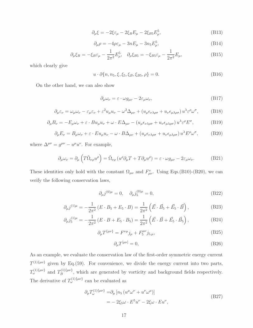
∂µξ = −2ξεµ − 2ξBEµ − 2ξB5E5µ, (B13)

∂µρ = −4ρεµ − 3nEµ − 3n5E5µ, (B14)

∂µξB = −ξBεµ −1

2π2E5

µ, ∂µξB5 = −ξB5εµ −1

2π2Eµ, (B15)

which clearly give

u · ∂n, n5, ξ, ξ5, ξB, ξB5, ρ = 0. (B16)

On the other hand, we can also show

∂µων = ε · ωgµν − 2εµων , (B17)

∂µεν = ωµων − εµεν + ε2uµuν − ω2∆µν + (uµǫνλρσ + uνǫµλρσ) uλερωσ, (B18)

∂µBν = −Eµων + ε · Buµuν + ω · E∆µν − (uµǫνλρσ + uνǫµλρσ) uλερEσ, (B19)

∂µEν = Bµων + ε · Euµuν − ω · B∆µν + (uµǫνλρσ + uνǫµλρσ)uλEρωσ, (B20)

where ∆µν = gµν − uµuν. For example,

∂µων = ∂µ

(

T Ωνρuρ)

= Ωνρ (uρ∂µT + T∂µu

ρ) = ε · ωgµν − 2εµων . (B21)

These identities only hold with the constant Ωµν and F sµν . Using Eqs.(B10)-(B20), we can

verify the following conservation laws,

∂µj(0)µ = 0, ∂µj

(0)µ5 = 0, (B22)

∂µj(1)µ = −

1

2π2(E · B5 + E5 ·B) =

1

2π2

(

~E · ~B5 + ~E5 · ~B)

, (B23)

∂µj(1)µ5 = −

1

2π2(E · B + E5 · B5) =

1

2π2

(

~E · ~B + ~E5 · ~B5

)

, (B24)

∂µTµν = F νµjµ + F µν

5 j5,µ, (B25)

∂µT[µν] = 0, (B26)

As an example, we evaluate the conservation law of the first-order symmetric energy current

T (1)µν given by Eq.(59). For convenience, we divide the energy current into two parts,

T(1)µνω and T

(1)µνB , which are generated by vorticity and background fields respectively.

The derivative of T(1)µνω can be evaluated as

∂µT(1)µνω =∂µ [n5 (u

µων + uνωµ)]

=− 2ξ5ω ·E5uν − 2ξω · Euν ,(B27)

17

while the derivative of T(1)µνB is

∂µT(1)µνB =∂µ

[

ξ

2(uµBν + uνBµ) +

ξ52(uµBν

5 + uνBµ5 )

]

=ξω · Euν + ξ5ω · E5uν + ξǫνµρσω

µuρBσ + ξ5ǫνµρσωµuρBσ

5

− uνE · (ξBB + ξB5B5)− uνE5 · (ξB5B + ξBB5),

(B28)

Then we can verify the conservation law of the first-order symmetric energy-momentum

tensor:

∂µT(1)µν =∂µT

(1)µνω + ∂µT

(1)µνB

=− uνE · j − uνE5 · j5 + ξǫνµρσωµuρBσ + ξ5ǫνµρσω

µuρBσ5

=F νµjµ + F νµ5 j5,µ,

(B29)

where we have used the decomposition of Eq.(41) in the third line.

In addition to the conservation of currents and energy-momentum tensor, we can also

obtain a relation between T (1)[µν] and spin tensor Sλµν . The latter is determined by the axial

current as

Sλµν =1

2ǫηλµνj5η. (B30)

Integrating Eq.(13) over ks, we identify the first two terms as T(1)[µν]s . The last term gives

s2ǫµναβ∂αj

sβ, while the term dependent on As

µ inside ∇sµ simply drops out as a total derivative

term. By taking the sum of right and left handed contributions, we arrive at

T (1)[µν] = ∂λSλµν . (B31)

ACKNOWLEDGMENTS

This work is in part supported by NSFC under Grant Nos 12075328, 11735007 and

11675274.

[1] Dam Thanh Son and Naoki Yamamoto. Kinetic theory with Berry curvature from quantum

field theories. Phys. Rev. D, 87(8):085016, 2013.

[2] M. A. Stephanov and Y. Yin. Chiral Kinetic Theory. Phys. Rev. Lett., 109:162001, 2012.

18

[3] Shi Pu, Jian-hua Gao, and Qun Wang. A consistent description of kinetic equation with

triangle anomaly. Phys. Rev. D, 83:094017, 2011.

[4] Jiunn-Wei Chen, Shi Pu, Qun Wang, and Xin-Nian Wang. Berry Curvature and Four-

Dimensional Monopoles in the Relativistic Chiral Kinetic Equation. Phys. Rev. Lett.,

110(26):262301, 2013.

[5] Yoshimasa Hidaka, Shi Pu, and Di-Lun Yang. Relativistic Chiral Kinetic Theory from Quan-

tum Field Theories. Phys. Rev. D, 95(9):091901, 2017.

[6] Cristina Manuel and Juan M. Torres-Rincon. Kinetic theory of chiral relativistic plasmas and

energy density of their gauge collective excitations. Phys. Rev. D, 89(9):096002, 2014.

[7] Cristina Manuel and Juan M. Torres-Rincon. Chiral transport equation from the quantum

Dirac Hamiltonian and the on-shell effective field theory. Phys. Rev. D, 90(7):076007, 2014.

[8] Anping Huang, Shuzhe Shi, Yin Jiang, Jinfeng Liao, and Pengfei Zhuang. Complete and

Consistent Chiral Transport from Wigner Function Formalism. Phys. Rev. D, 98(3):036010,

2018.

[9] Stefano Carignano, Cristina Manuel, and Juan M. Torres-Rincon. Consistent relativistic chiral

kinetic theory: A derivation from on-shell effective field theory. Phys. Rev. D, 98(7):076005,

2018.

[10] Jian-Hua Gao, Zuo-Tang Liang, Qun Wang, and Xin-Nian Wang. Disentangling covariant

Wigner functions for chiral fermions. Phys. Rev. D, 98(3):036019, 2018.

[11] Ziyue Wang, Xingyu Guo, Shuzhe Shi, and Pengfei Zhuang. Mass Correction to Chiral Kinetic

Equations. Phys. Rev. D, 100(1):014015, 2019.

[12] Shu Lin and Aradhya Shukla. Chiral Kinetic Theory from Effective Field Theory Revisited.

JHEP, 06:060, 2019.

[13] Jian-Hua Gao, Zuo-Tang Liang, and Qun Wang. Dirac sea and chiral anomaly in the quantum

kinetic theory. Phys. Rev. D, 101(9):096015, 2020.

[14] Tomoya Hayata, Yoshimasa Hidaka, and Kazuya Mameda. Second order chiral kinetic theory

under gravity and antiparallel charge-energy flow. JHEP, 05:023, 2021.

[15] Shi-Zheng Yang, Jian-Hua Gao, Zuo-Tang Liang, and Qun Wang. Second-order charge cur-

rents and stress tensor in a chiral system. Phys. Rev. D, 102(11):116024, 2020.

[16] Shu Lin and Lixin Yang. Chiral kinetic theory from Landau level basis. Phys. Rev. D,

101(3):034006, 2020.

19

[17] Shu Lin and Lixin Yang. Magneto-vortical effect in strong magnetic field. JHEP, 06:054, 2021.

[18] Xiao-Li Luo and Jian-Hua Gao. Covariant Chiral Kinetic Equation in Non-Abelian Gauge

field from ”covariant gradient expansion”. 7 2021.

[19] Dmitri Kharzeev. Parity violation in hot QCD: Why it can happen, and how to look for it.

Phys. Lett. B, 633:260–264, 2006.

[20] D. Kharzeev and A. Zhitnitsky. Charge separation induced by P-odd bubbles in QCD matter.

Nucl. Phys. A, 797:67–79, 2007.

[21] Kenji Fukushima, Dmitri E. Kharzeev, and Harmen J. Warringa. The Chiral Magnetic Effect.

Phys. Rev. D, 78:074033, 2008.

[22] Johanna Erdmenger, Michael Haack, Matthias Kaminski, and Amos Yarom. Fluid dynamics

of R-charged black holes. JHEP, 01:055, 2009.

[23] Nabamita Banerjee, Jyotirmoy Bhattacharya, Sayantani Bhattacharyya, Suvankar Dutta,

R. Loganayagam, and P. Surowka. Hydrodynamics from charged black branes. JHEP, 01:094,

2011.

[24] Yasha Neiman and Yaron Oz. Relativistic Hydrodynamics with General Anomalous Charges.

JHEP, 03:023, 2011.

[25] Karl Landsteiner, Eugenio Megias, and Francisco Pena-Benitez. Gravitational Anomaly and

Transport. Phys. Rev. Lett., 107:021601, 2011.

[26] Koichi Hattori, Yoshimasa Hidaka, and Di-Lun Yang. Axial Kinetic Theory and Spin Trans-

port for Fermions with Arbitrary Mass. Phys. Rev. D, 100(9):096011, 2019.

[27] Nora Weickgenannt, Xin-Li Sheng, Enrico Speranza, Qun Wang, and Dirk H. Rischke. Kinetic

theory for massive spin-1/2 particles from the Wigner-function formalism. Phys. Rev. D,

100(5):056018, 2019.

[28] Jian-Hua Gao and Zuo-Tang Liang. Relativistic Quantum Kinetic Theory for Massive

Fermions and Spin Effects. Phys. Rev. D, 100(5):056021, 2019.

[29] Yu-Chen Liu, Kazuya Mameda, and Xu-Guang Huang. Covariant Spin Kinetic Theory I:

Collisionless Limit. Chin. Phys. C, 44(9):094101, 2020. [Erratum: Chin.Phys.C 45, 089001

(2021)].

[30] Xingyu Guo. Massless Limit of Transport Theory for Massive Fermions. Chin. Phys. C,

44(10):104106, 2020.

[31] Jian-Hua Gao, Guo-Liang Ma, Shi Pu, and Qun Wang. Recent developments in chiral and

20

spin polarization effects in heavy-ion collisions. Nucl. Sci. Tech., 31(9):90, 2020.

[32] Jun-jie Zhang, Ren-hong Fang, Qun Wang, and Xin-Nian Wang. A microscopic description

for polarization in particle scatterings. Phys. Rev. C, 100(6):064904, 2019.

[33] Shiyong Li and Ho-Ung Yee. Quantum Kinetic Theory of Spin Polarization of Massive Quarks

in Perturbative QCD: Leading Log. Phys. Rev. D, 100(5):056022, 2019.

[34] Stefano Carignano, Cristina Manuel, and Juan M. Torres-Rincon. Chiral kinetic theory from

the on-shell effective field theory: Derivation of collision terms. Phys. Rev. D, 102(1):016003,

2020.

[35] Di-Lun Yang, Koichi Hattori, and Yoshimasa Hidaka. Effective quantum kinetic theory for

spin transport of fermions with collsional effects. JHEP, 07:070, 2020.

[36] Ziyue Wang, Xingyu Guo, and Pengfei Zhuang. Local Equilibrium Spin Distribution From

Detailed Balance. 9 2020.

[37] Shuzhe Shi, Charles Gale, and Sangyong Jeon. From chiral kinetic theory to relativistic viscous

spin hydrodynamics. Phys. Rev. C, 103(4):044906, 2021.

[38] Nora Weickgenannt, Enrico Speranza, Xin-li Sheng, Qun Wang, and Dirk H. Rischke. Gen-

erating Spin Polarization from Vorticity through Nonlocal Collisions. Phys. Rev. Lett.,

127(5):052301, 2021.

[39] Defu Hou and Shu Lin. Polarization Rotation of Chiral Fermions in Vortical Fluid. Phys.

Lett. B, 818:136386, 2021.

[40] Naoki Yamamoto and Di-Lun Yang. Chiral Radiation Transport Theory of Neutrinos.

Astrophys. J., 895(1):56, 2020.

[41] Nora Weickgenannt, Enrico Speranza, Xin-li Sheng, Qun Wang, and Dirk H. Rischke. Deriva-

tion of the nonlocal collision term in the relativistic Boltzmann equation for massive spin-1/2

particles from quantum field theory. Phys. Rev. D, 104(1):016022, 2021.

[42] Xin-Li Sheng, Nora Weickgenannt, Enrico Speranza, Dirk H. Rischke, and Qun Wang.

From Kadanoff-Baym to Boltzmann equations for massive spin-1/2 fermions. Phys. Rev.

D, 104(1):016029, 2021.

[43] Ziyue Wang and Pengfei Zhuang. Damping and polarization rates in near equilibrium state.

5 2021.

[44] Shu Lin. Quantum Kinetic Theory for Quantum Electrodynamics. 9 2021.

[45] Xu-Guang Huang and Andrey V. Sadofyev. Chiral Vortical Effect For An Arbitrary Spin.

21

JHEP, 03:084, 2019.

[46] Xu-Guang Huang, Pavel Mitkin, Andrey V. Sadofyev, and Enrico Speranza. Zilch Vortical

Effect, Berry Phase, and Kinetic Theory. JHEP, 10:117, 2020.

[47] Koichi Hattori, Yoshimasa Hidaka, Naoki Yamamoto, and Di-Lun Yang. Wigner functions

and quantum kinetic theory of polarized photons. JHEP, 02:001, 2021.

[48] Daisuke Satow. Nonlinear electromagnetic response in quark-gluon plasma. Phys. Rev. D,

90(3):034018, 2014.

[49] E. V. Gorbar, D. O. Rybalka, and I. A. Shovkovy. Second-order dissipative hydrodynamics

for plasma with chiral asymmetry and vorticity. Phys. Rev. D, 95(9):096010, 2017.

[50] M. Buzzegoli, E. Grossi, and F. Becattini. General equilibrium second-order hydrodynamic

coefficients for free quantum fields. JHEP, 10:091, 2017. [Erratum: JHEP 07, 119 (2018)].

[51] M. Buzzegoli and F. Becattini. General thermodynamic equilibrium with axial chemical po-

tential for the free Dirac field. JHEP, 12:002, 2018.

[52] Wojciech Florkowski, Avdhesh Kumar, and Radoslaw Ryblewski. Relativistic hydrodynamics

for spin-polarized fluids. Prog. Part. Nucl. Phys., 108:103709, 2019.

[53] Samapan Bhadury, Wojciech Florkowski, Amaresh Jaiswal, Avdhesh Kumar, and Radoslaw

Ryblewski. Relativistic dissipative spin dynamics in the relaxation time approximation. Phys.

Lett. B, 814:136096, 2021.

[54] Hao-Hao Peng, Jun-Jie Zhang, Xin-Li Sheng, and Qun Wang. Ideal spin hydrodynamics from

Wigner function approach. 7 2021.

[55] The derivation based on responses works for more general systems where kinetic description

might not apply, see [58, 63–65] and references therein.

[56] Dam T. Son and Piotr Surowka. Hydrodynamics with Triangle Anomalies. Phys. Rev. Lett.,

103:191601, 2009.

[57] A. A. Zyuzin, Si Wu, and A. A. Burkov. Weyl semimetal with broken time reversal and

inversion symmetries. Phys. Rev. B, 85:165110, 2012.

[58] Masaru Hongo, Xu-Guang Huang, Matthias Kaminski, Mikhail Stephanov, and Ho-Ung Yee.

Relativistic spin hydrodynamics with torsion and linear response theory for spin relaxation.

7 2021.

[59] Karl Landsteiner. Notes on Anomaly Induced Transport. Acta Phys. Polon. B, 47:2617, 2016.

[60] In the absence of collision term, the expansion in ∂X is equivalent to expansion in ~.

22

[61] Implicitly we assume that the fluid velocity is not redefined in the presence of external sources

including vector/axial gauge fields and vorticity. This chooses a particular hydrodynamic

frame, termed thermodynamic frame in literature [66].

[62] See [67] for the case with a background magnetic field.

[63] Nabamita Banerjee, Jyotirmoy Bhattacharya, Sayantani Bhattacharyya, Sachin Jain, Shiraz

Minwalla, and Tarun Sharma. Constraints on Fluid Dynamics from Equilibrium Partition

Functions. JHEP, 09:046, 2012.

[64] Juan Hernandez and Pavel Kovtun. Relativistic magnetohydrodynamics. JHEP, 05:001, 2017.

[65] A. D. Gallegos, U. Gursoy, and A. Yarom. Hydrodynamics of spin currents. SciPost Phys.,

11:041, 2021.

[66] Kristan Jensen, Matthias Kaminski, Pavel Kovtun, Rene Meyer, Adam Ritz, and Amos

Yarom. Towards hydrodynamics without an entropy current. Phys. Rev. Lett., 109:101601,

2012.

[67] Yanyan Bu and Shu Lin. Magneto-vortical effect in strongly coupled plasma. Eur. Phys. J.

C, 80(5):401, 2020.

23