Quantum Lattice Models&

Introduction to Exact Diagonalization

ALPS User Workshop CSCS Manno, 28/9/2004

Andreas LäuchliIRRMA – EPF Lausanne

!=! EH

28/9/2004 ALPS User Workshop Manno 2

Outline of this lecture:

Quantum Lattice Models Lattices and Models in general and in ALPS

Exact Diagonalization (ED) The Method and its applications Ingredients

ED Extensions Finite Temperature Lanczos Methods Contractor Renormalization (CORE)

Quantum Lattice Models

kagome lattice Volborthite

28/9/2004 ALPS User Workshop Manno 4

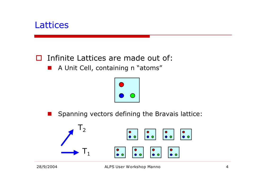
Lattices

Infinite Lattices are made out of: A Unit Cell, containing n “atoms”

Spanning vectors defining the Bravais lattice:

T1

T2

28/9/2004 ALPS User Workshop Manno 5

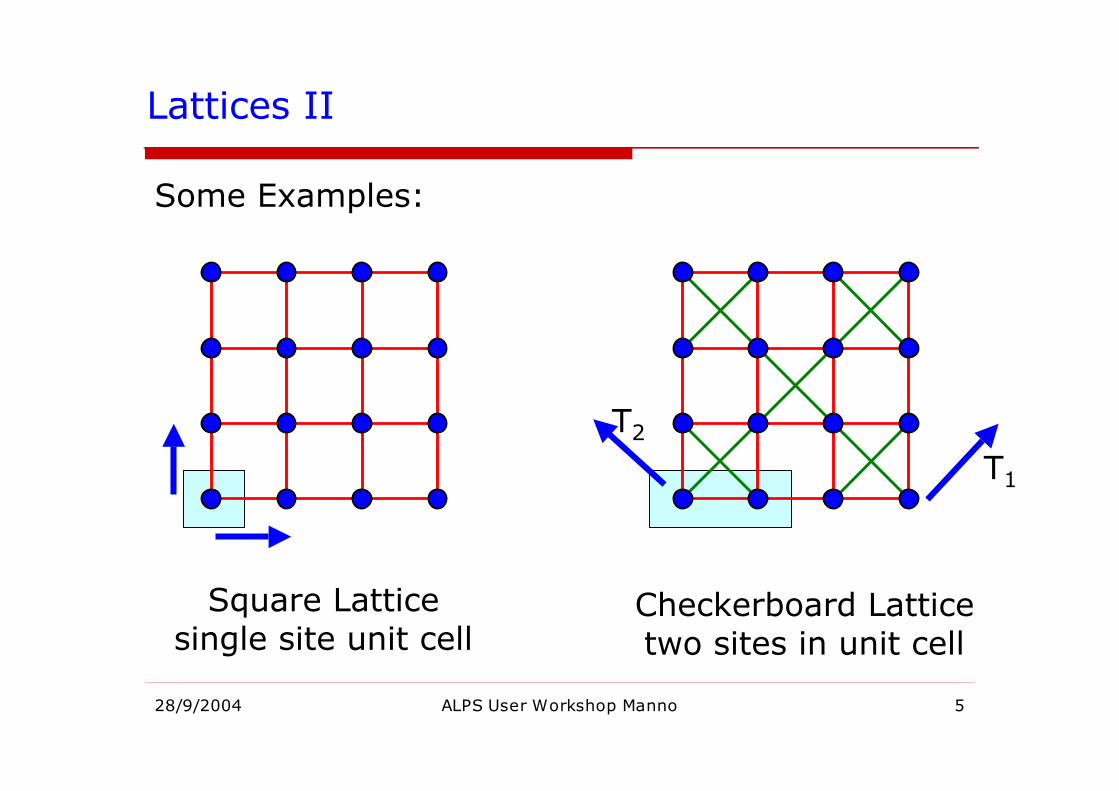
Square Latticesingle site unit cell

Lattices II

Some Examples:

Checkerboard Latticetwo sites in unit cell

T1

T2

28/9/2004 ALPS User Workshop Manno 6

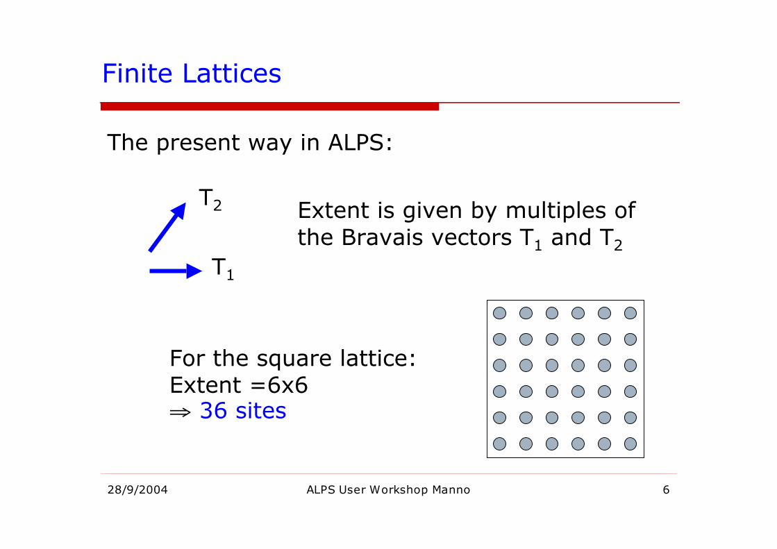
Finite Lattices

The present way in ALPS:

T1

T2 Extent is given by multiples ofthe Bravais vectors T1 and T2

For the square lattice:Extent =6x6⇒ 36 sites

28/9/2004 ALPS User Workshop Manno 7

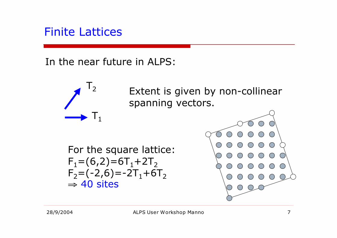
Finite Lattices

In the near future in ALPS:

T1

T2 Extent is given by non-collinearspanning vectors.

For the square lattice:F1=(6,2)=6T1+2T2F2=(-2,6)=-2T1+6T2⇒ 40 sites

28/9/2004 ALPS User Workshop Manno 8

Models

Many Body Lattice Models

Single Particle Lattice Models

Constrained Models

28/9/2004 ALPS User Workshop Manno 9

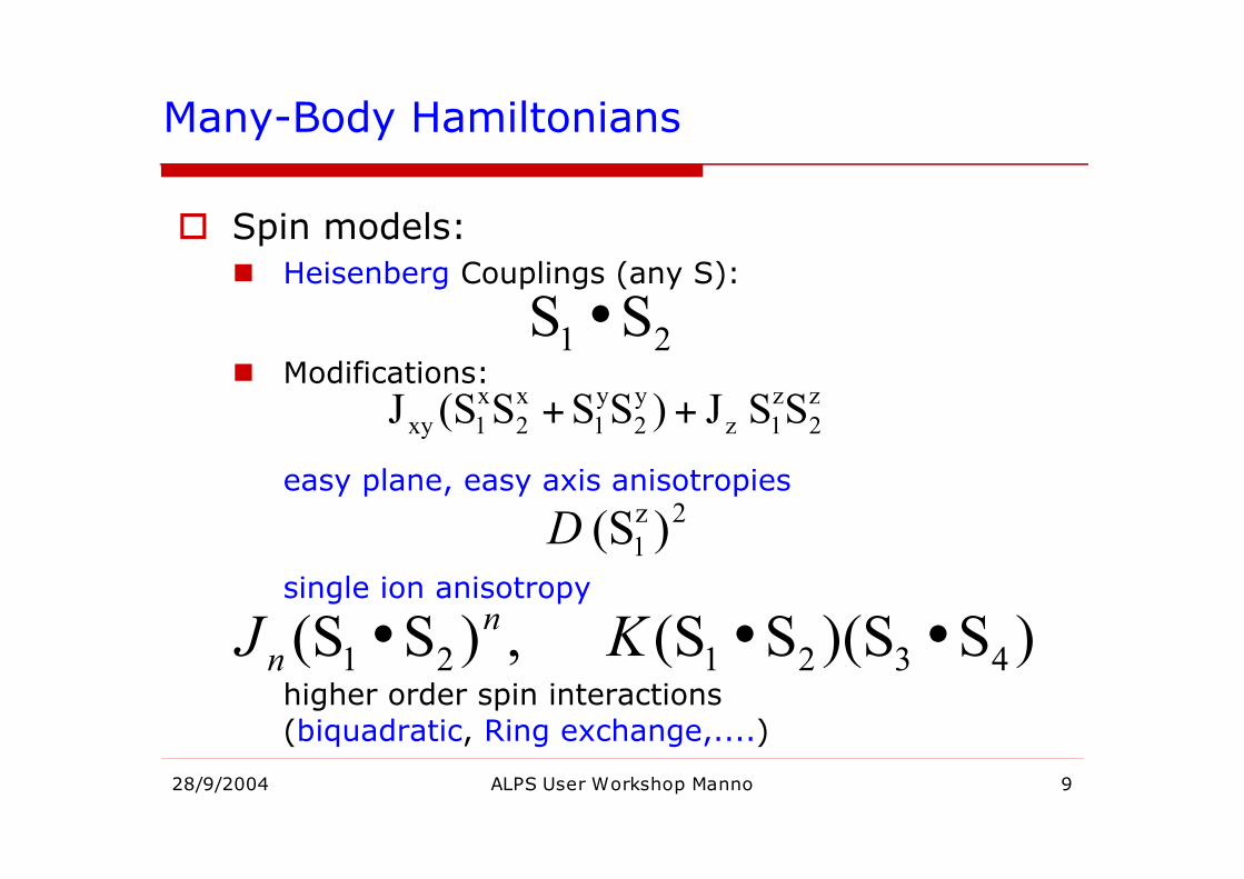
Many-Body Hamiltonians

Spin models: Heisenberg Couplings (any S):

Modifications:

easy plane, easy axis anisotropies

single ion anisotropy

higher order spin interactions(biquadratic, Ring exchange,....)

21SS •

2z

1 )(S D

)S(S)S(S ,)S(S 432121 ••• KJn

n

z

2

z

1z

y

2

y

1

x

2

x

1xy SS J)SSS(SJ ++

28/9/2004 ALPS User Workshop Manno 10

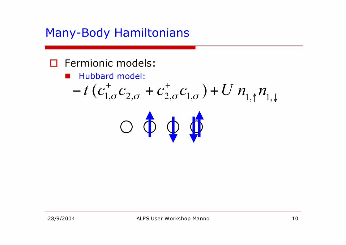
Many-Body Hamiltonians

Fermionic models: Hubbard model:

!"

++++#

,1,1,1,2,2,1 )( nnUcccct $$$$

28/9/2004 ALPS User Workshop Manno 11

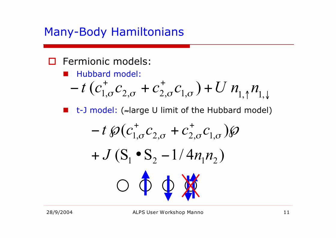
Many-Body Hamiltonians

Fermionic models: Hubbard model:

t-J model: (≈large U limit of the Hubbard model)

!"

++++#

,1,1,1,2,2,1 )( nnUcccct $$$$

)4/1S(S

)(

2121

,1,2,2,1

nnJ

cccct

!•+

"+"!++

####

28/9/2004 ALPS User Workshop Manno 12

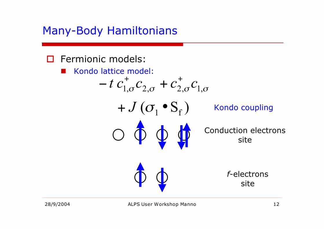
Many-Body Hamiltonians

Fermionic models: Kondo lattice model:

)S(

f1

,1,2,2,1

•+

+!++

"

""""

J

cccct

Conduction electronssite

f-electronssite

Kondo coupling

28/9/2004 ALPS User Workshop Manno 13

Single Particle Models

Disordered potentials and hoppings⇒ Anderson Localization

Hopping phases⇒ Hofstadter Butterfly

Jordan-Wigner transformation⇒ Disordered XX-spin chains

28/9/2004 ALPS User Workshop Manno 14

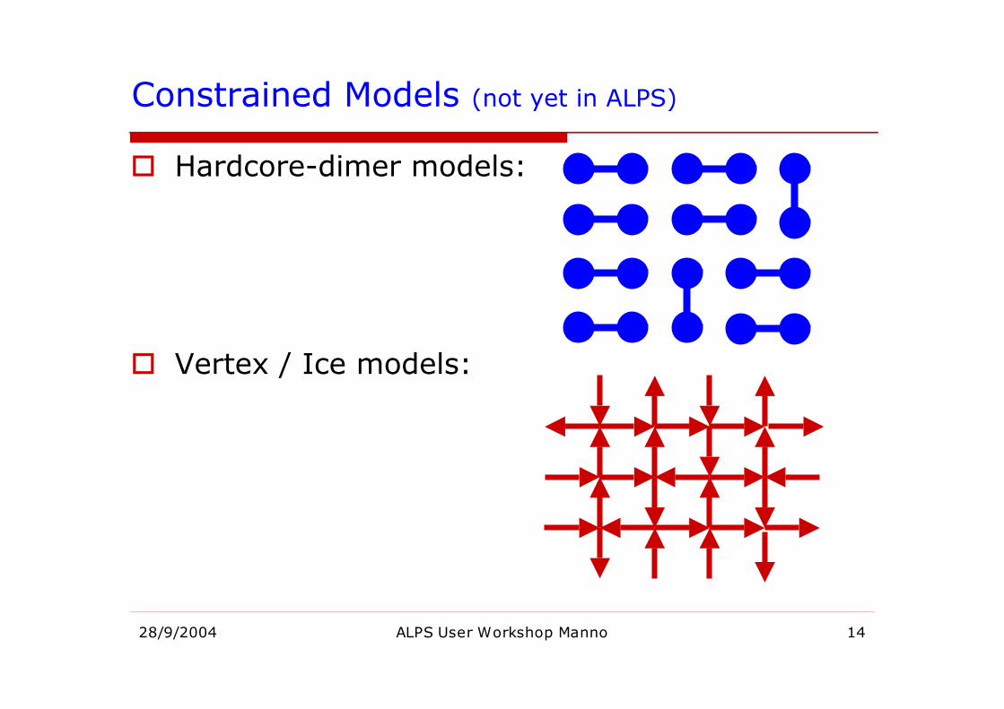
Constrained Models (not yet in ALPS)

Hardcore-dimer models:

Vertex / Ice models:

Exact Diagonalization

!=! EH

28/9/2004 ALPS User Workshop Manno 16

Exact Diagonalization

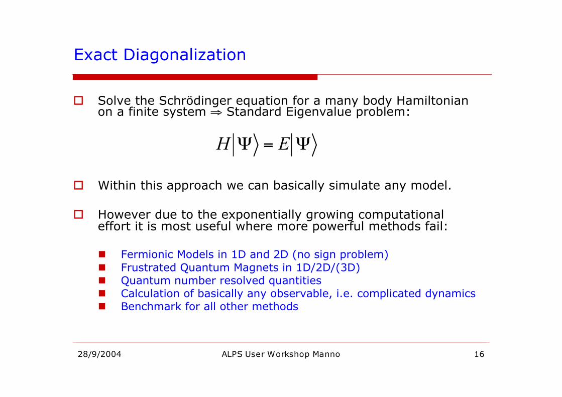
Solve the Schrödinger equation for a many body Hamiltonianon a finite system ⇒ Standard Eigenvalue problem:

Within this approach we can basically simulate any model.

However due to the exponentially growing computationaleffort it is most useful where more powerful methods fail:

Fermionic Models in 1D and 2D (no sign problem) Frustrated Quantum Magnets in 1D/2D/(3D) Quantum number resolved quantities Calculation of basically any observable, i.e. complicated dynamics Benchmark for all other methods

!=! EH

28/9/2004 ALPS User Workshop Manno 17

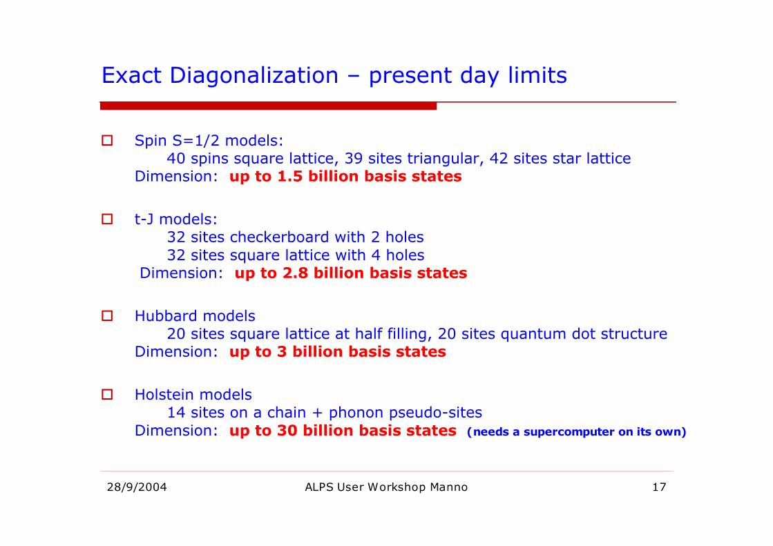
Exact Diagonalization – present day limits

Spin S=1/2 models:40 spins square lattice, 39 sites triangular, 42 sites star lattice

Dimension: up to 1.5 billion basis states

t-J models:32 sites checkerboard with 2 holes32 sites square lattice with 4 holes

Dimension: up to 2.8 billion basis states

Hubbard models20 sites square lattice at half filling, 20 sites quantum dot structure

Dimension: up to 3 billion basis states

Holstein models14 sites on a chain + phonon pseudo-sites

Dimension: up to 30 billion basis states (needs a supercomputer on its own)

28/9/2004 ALPS User Workshop Manno 18

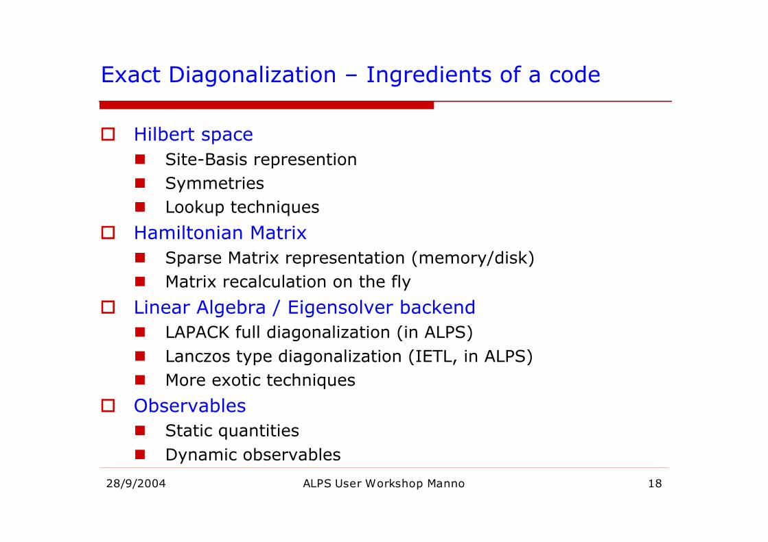
Exact Diagonalization – Ingredients of a code

Hilbert space Site-Basis represention Symmetries Lookup techniques

Hamiltonian Matrix Sparse Matrix representation (memory/disk) Matrix recalculation on the fly

Linear Algebra / Eigensolver backend LAPACK full diagonalization (in ALPS) Lanczos type diagonalization (IETL, in ALPS) More exotic techniques

Observables Static quantities Dynamic observables

28/9/2004 ALPS User Workshop Manno 19

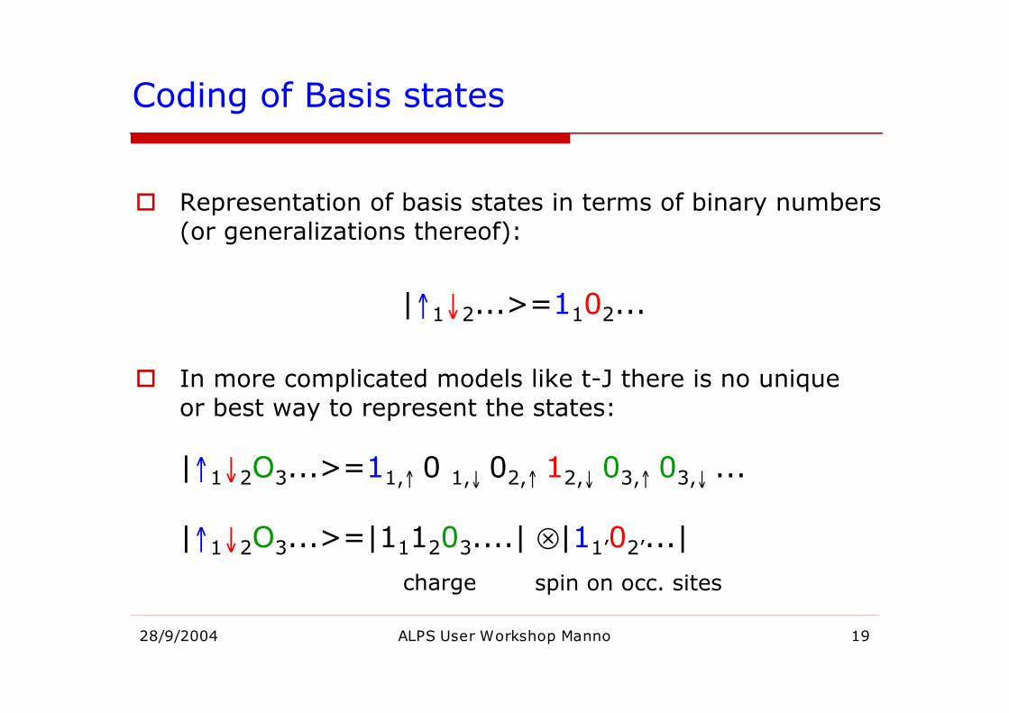
Coding of Basis states

Representation of basis states in terms of binary numbers(or generalizations thereof):

|↑1↓2...>=1102...

In more complicated models like t-J there is no uniqueor best way to represent the states:

|↑1↓2O3...>=11,↑ 0 1,↓ 02,↑ 12,↓ 03,↑ 03,↓ ...

|↑1↓2O3...>=|111203....| ⊗|11’02’...|charge spin on occ. sites

28/9/2004 ALPS User Workshop Manno 20

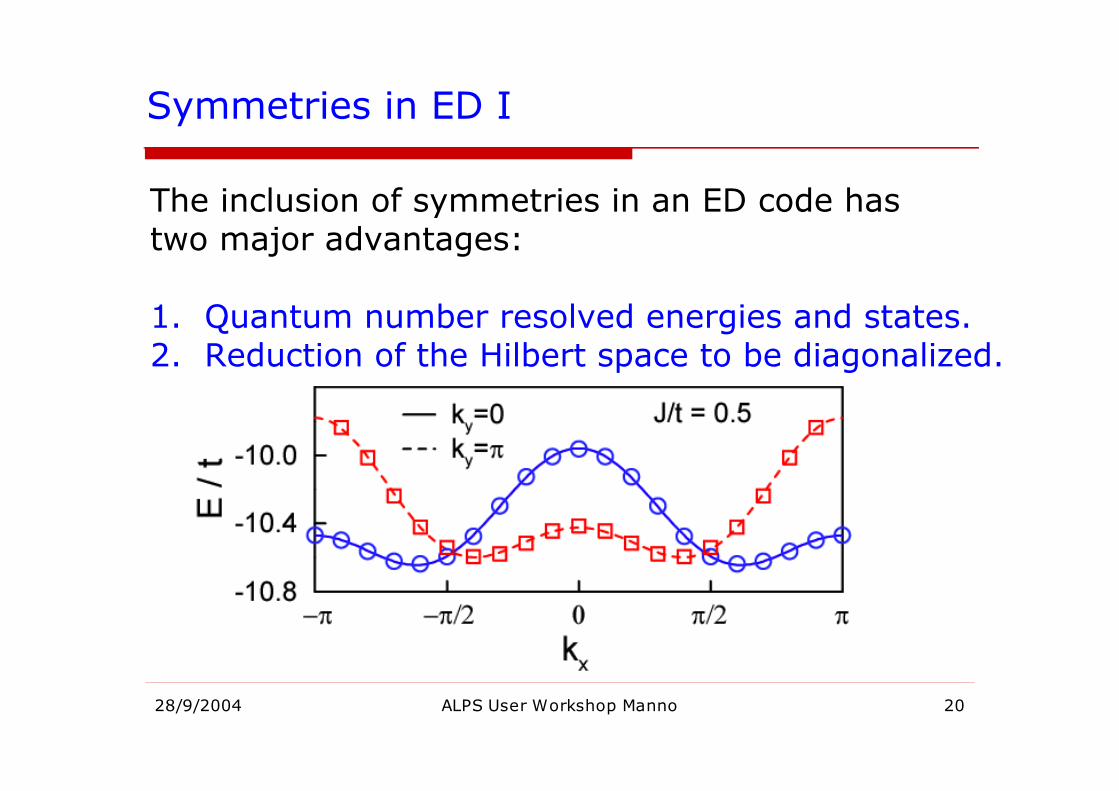
Symmetries in ED I

The inclusion of symmetries in an ED code has two major advantages:

1. Quantum number resolved energies and states.2. Reduction of the Hilbert space to be diagonalized.

28/9/2004 ALPS User Workshop Manno 21

Symmetries in ED II

U(1) related symmetries: Conservation of particle number(s) Conservation of total Sz

Spatial symmetry groups: Translation symmetry (abelian symmetry, therefore 1D irreps) Pointgroup symmetries (in general non-abelian)

SU(2) symmetry Difficult to implement together with spatial symmetries For Sz=0 an operation called “spin inversion” splits the

Hilbert space in even and odd spin sectors.

28/9/2004 ALPS User Workshop Manno 22

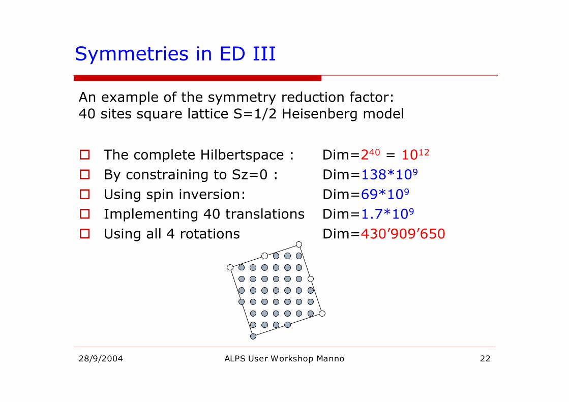
The complete Hilbertspace : Dim=240 = 1012

By constraining to Sz=0 : Dim=138*109

Using spin inversion: Dim=69*109

Implementing 40 translations Dim=1.7*109

Using all 4 rotations Dim=430’909’650

Symmetries in ED III

An example of the symmetry reduction factor:40 sites square lattice S=1/2 Heisenberg model

28/9/2004 ALPS User Workshop Manno 23

Linear Algebra in Exact Diagonalization I

Lanczos algorithm:C. Lanczos, , J. Res. Natl. Bur. Stand. 45, 255 (1950).

Iterative “Krylov”-space method which bringsmatrices into tridiagonal form. Method of choicein many large-scale ED programs. Very rapid convergence. Memory requirements between 2 and 4 vectors. Numerically unstable, but with suitable techniques

this is under control (Cullum and Willoughby). Easy to implement.

Z. Bai, J. Demmel, J. Dongarra, A. Ruhe and H. van der Vorst (eds), Templates for the solution of Algebraic Eigenvalue Problems:

A Practical Guide . SIAM, Philadelphia, 2000http://www.cs.ucdavis.edu/~bai/ET/contents.html

28/9/2004 ALPS User Workshop Manno 24

Jacobi-Davidson Algorithm:E. R. Davidson, Comput. Phys. 7, 519 (1993).

Rapid convergence, especially for diagonallydominant matrices (Hubbard model).

Varying number of vectors in memory. Often used in DMRG programs as well.

“modified Lanczos” algorithm:E. Gagliano, et al. Phys. Rev. B 34, 1677 (1986).

actually more like a Power-method,therefore rather slow convergence.

needs only two vectors in memory. At each step the approximate groundstate

wavefunction is available. Difficult to get excited states.

Linear Algebra in Exact Diagonalization II

28/9/2004 ALPS User Workshop Manno 25

Lanczos Algorithm I

!!!!!

"

#

$$$$$

%

&

=

n

n

a

ab

bab

ba

T

...

...32

221

11

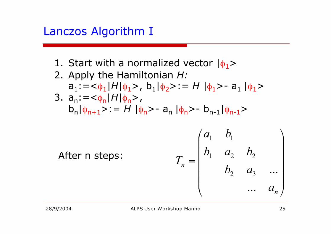
1. Start with a normalized vector |φ1>2. Apply the Hamiltonian H:

a1:=<φ1|H|φ1>, b1|φ2>:= H |φ1>- a1 |φ1>3. an:=<φn|H|φn>,

bn|φn+1>:= H |φn>- an |φn>- bn-1|φn-1>

After n steps:

28/9/2004 ALPS User Workshop Manno 26

Lanczos Algorithm II

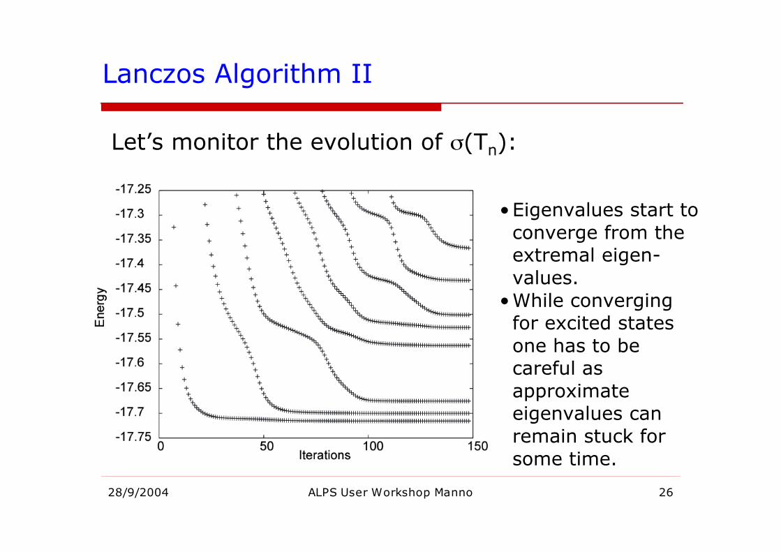
Let’s monitor the evolution of σ(Tn):

•Eigenvalues start toconverge from theextremal eigen-values.

•While convergingfor excited statesone has to becareful asapproximateeigenvalues canremain stuck forsome time.

28/9/2004 ALPS User Workshop Manno 27

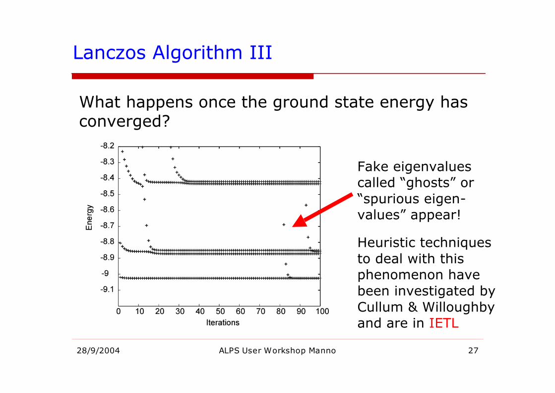
Lanczos Algorithm III

What happens once the ground state energy hasconverged?

Fake eigenvaluescalled “ghosts” or“spurious eigen-values” appear!

Heuristic techniquesto deal with thisphenomenon havebeen investigated byCullum & Willoughbyand are in IETL

28/9/2004 ALPS User Workshop Manno 28

Observables in ED

Energy, as function of quantum numbers! “Diagonal” correlation functions:

easy to calculate in the chosen basis, i.e. Sz-correlations,density correlations, string order parameter,...

Off-diagonal correlations: Sx-Sx, kinetic energy Higher order correlation functions:

dimer-dimer correlations, vector chirality correlationfunctions, pairing correlations,...

Dynamical correlations of all sorts (⇒ talk by D. Poilblanc)

Note that evaluation of complicated observablescan become as important as obtaining the groundstate!

Note also that in general the precision on correlationfunctions is not as high as the energy!

28/9/2004 ALPS User Workshop Manno 29

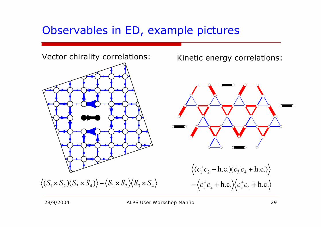
Observables in ED, example pictures

43214321 ))(( SSSSSSSS !!"!!

Vector chirality correlations: Kinetic energy correlations:

h.c.h.c.

)h.c.)(h.c.(

4321

4321

++!

++

++

++

cccc

cccc

28/9/2004 ALPS User Workshop Manno 30

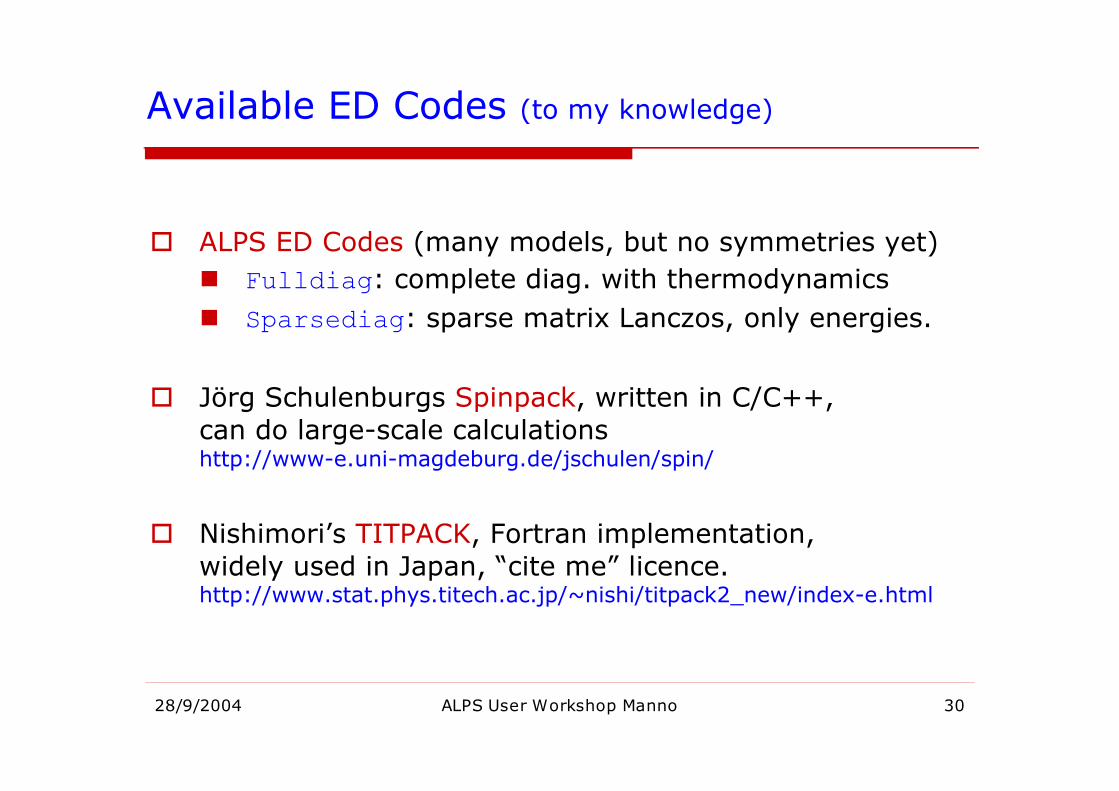
Available ED Codes (to my knowledge)

ALPS ED Codes (many models, but no symmetries yet) Fulldiag: complete diag. with thermodynamics Sparsediag: sparse matrix Lanczos, only energies.

Jörg Schulenburgs Spinpack, written in C/C++,can do large-scale calculationshttp://www-e.uni-magdeburg.de/jschulen/spin/

Nishimori’s TITPACK, Fortran implementation,widely used in Japan, “cite me” licence.http://www.stat.phys.titech.ac.jp/~nishi/titpack2_new/index-e.html

Extensions of Exact Diagonalization

Finite Temperature Lanczos Methods:

Contractor Renormalization (CORE):

Extensions of Exact Diagonalization

Finite Temperature Lanczos Methods:• J. Jaklic and P. Prelovsek, Adv. Phys. 49, 1 (2000).• M. Aichhorn et al., Phys. Rev. B 67, 161103 (2003).

28/9/2004 ALPS User Workshop Manno 33

These methods (FTLM,LTLM) combine the Lanczosmethod and random sampling to go to larger systems.

For high to moderate temperatures these methodscan obtain results basically in the thermodynamiclimit.

The Low Temperature Lanczos Method can also go tolow temperatures to get correct results on a givensample. Finite size effects however persist.

Like the T=0 ED method it is most useful, where QMCor T-DMRG etc fail, such as frustrated and fermionicmodels.

Possibly in ALPS in the not so distant future...

Finite Temperature Lanczos Methods

Extensions of Exact Diagonalization

Contractor Renormalization (CORE):• C.J. Morningstar and M. Weinstein,

Phys. Rev. D 54 4131 (1996).• E. Altman and A. Auerbach,

Phys. Rev. B 65, 104508 (2002).• S. Capponi, A. Läuchli and M. Mambrini,

cond-mat/0404712, to be published in PRB

28/9/2004 ALPS User Workshop Manno 35

CORE – Basic Idea

Choose a suitable decomposition of yourlattice and keep a certain number of suitablestates

Determine the effective Hamiltonian byrequiring to reproduce the low energyspectrum of the non-truncated system onsmall clusters.

Simulate (or treat analytically) the neweffective Hamiltonian.

28/9/2004 ALPS User Workshop Manno 36

Contractor Renormalization

How to choose the states to keep?

Low energy states of the local building block

States with the highest weight in the local density matrix

28/9/2004 ALPS User Workshop Manno 37

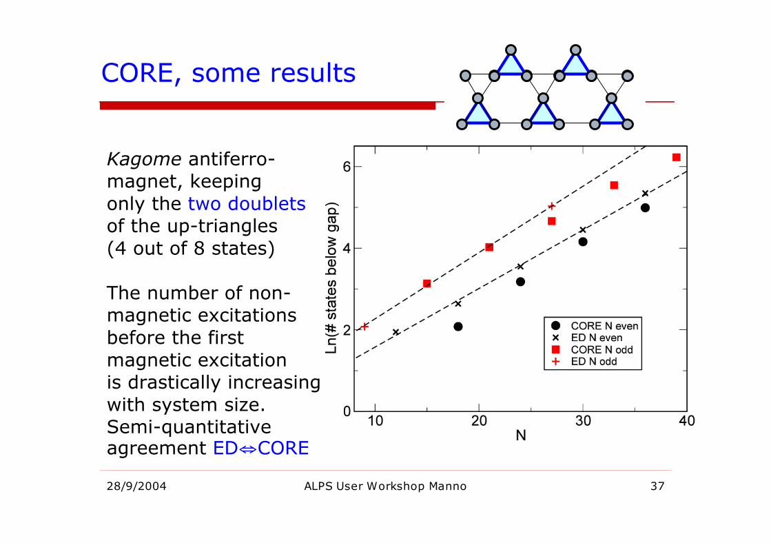
CORE, some results

Kagome antiferro-magnet, keepingonly the two doubletsof the up-triangles(4 out of 8 states)

The number of non-magnetic excitationsbefore the first magnetic excitationis drastically increasingwith system size.Semi-quantitativeagreement ED⇔CORE