Embed Size (px)
Citation preview
Quantum Learning Algorithms
and Post-Quantum Cryptography∗
Alexander M. Poremba
1 QMATH, Department of Mathematical Sciences, University of Copenhagen,
1165 Copenhagen, Denmark.
2 Department of Physics and Astronomy, University of Heidelberg,
69047 Heidelberg, Germany.
Abstract. Quantum algorithms have demonstrated promising speed-ups over
classical algorithms in the context of computational learning theory - despite the
presence of noise. In this work, we give an overview of recent quantum speed-ups,
revisit the Bernstein-Vazirani algorithm in a new learning problem extension over
an arbitrary cyclic group and discuss recent applications in cryptography, such as
the Learning with Errors problem.
We turn to post-quantum cryptography and investigate attacks in which an ad-
versary is given quantum access to a classical encryption scheme. In particular, we
consider new notions of security under non-adaptive quantum chosen-ciphertext
attacks and propose symmetric-key encryption schemes based on quantum-secure
pseudorandom functions that fulfil our definitions. In order to prove security, we
introduce a novel relabeling game and show that, in an oracle model, no quantum
algorithm making superposition queries can reliably distinguish between the class
of functions that are randomly relabeled at a small subset of the domain.
Finally, we discuss current progress in quantum computing technology, particu-
larly with regard to the ion-trap architecture, as well as the implementation of
quantum algorithms. Moreover, we shed light on the relevance and effectiveness
of common noise models adopted in computational learning theory.
∗This work was carried out as part of my Master’s thesis at the University of Heidelberg.
Contact: [email protected]
arX
iv:1
712.
0928
9v2
[qu
ant-
ph]
1 J
an 2
018
Principal supervisor:
Gorjan Alagic,
Joint Center for Quantum Information
and Computer Science,
University of Maryland, College Park, MD
Co-supervisor:
Thomas Gasenzer,
Kirchhoff-Institute for Physics,
University of Heidelberg, Germany.
Table of Contents
1 List of Abbreviations . . . . . . . . . . . . . . . . . . . . . . . . . . . . . . . . . . . . . . . . . . . . . . . . . . . . . . . . . 5
2 Introduction . . . . . . . . . . . . . . . . . . . . . . . . . . . . . . . . . . . . . . . . . . . . . . . . . . . . . . . . . . . . . . . . 6
3 Main Results . . . . . . . . . . . . . . . . . . . . . . . . . . . . . . . . . . . . . . . . . . . . . . . . . . . . . . . . . . . . . . . . 11
4 Cryptography . . . . . . . . . . . . . . . . . . . . . . . . . . . . . . . . . . . . . . . . . . . . . . . . . . . . . . . . . . . . . . . 15
4.1 Preliminaries . . . . . . . . . . . . . . . . . . . . . . . . . . . . . . . . . . . . . . . . . . . . . . . . . . . . . . . . . . . 15
4.2 Symmetric-Key Cryptography . . . . . . . . . . . . . . . . . . . . . . . . . . . . . . . . . . . . . . . . . . . . 16
4.3 Security Notions . . . . . . . . . . . . . . . . . . . . . . . . . . . . . . . . . . . . . . . . . . . . . . . . . . . . . . . . 17
Computational Security . . . . . . . . . . . . . . . . . . . . . . . . . . . . . . . . . . . . . . . . . . . . . . . . . 17
Computational Indistinguishability. . . . . . . . . . . . . . . . . . . . . . . . . . . . . . . . . . . . . . . . 17
Semantic Security. . . . . . . . . . . . . . . . . . . . . . . . . . . . . . . . . . . . . . . . . . . . . . . . . . . . . . . 19
4.4 Pseudorandom Functions . . . . . . . . . . . . . . . . . . . . . . . . . . . . . . . . . . . . . . . . . . . . . . . . 20
4.5 Learning with Errors . . . . . . . . . . . . . . . . . . . . . . . . . . . . . . . . . . . . . . . . . . . . . . . . . . . . 21
Decision Learning with Errors. . . . . . . . . . . . . . . . . . . . . . . . . . . . . . . . . . . . . . . . . . . . 22
Symmetric-Key Constructions and Security. . . . . . . . . . . . . . . . . . . . . . . . . . . . . . . . . 22
Separation Result. . . . . . . . . . . . . . . . . . . . . . . . . . . . . . . . . . . . . . . . . . . . . . . . . . . . . . . 23
5 Quantum Computation . . . . . . . . . . . . . . . . . . . . . . . . . . . . . . . . . . . . . . . . . . . . . . . . . . . . . . . 25
5.1 Formalism . . . . . . . . . . . . . . . . . . . . . . . . . . . . . . . . . . . . . . . . . . . . . . . . . . . . . . . . . . . . . 25
5.2 Unitary Evolution . . . . . . . . . . . . . . . . . . . . . . . . . . . . . . . . . . . . . . . . . . . . . . . . . . . . . . 27
5.3 Quantum Measurement . . . . . . . . . . . . . . . . . . . . . . . . . . . . . . . . . . . . . . . . . . . . . . . . . . 28
5.4 Universal Quantum Gates . . . . . . . . . . . . . . . . . . . . . . . . . . . . . . . . . . . . . . . . . . . . . . . 29
5.5 The No-Cloning Theorem . . . . . . . . . . . . . . . . . . . . . . . . . . . . . . . . . . . . . . . . . . . . . . . . 31
5.6 The Quantum Circuit Model . . . . . . . . . . . . . . . . . . . . . . . . . . . . . . . . . . . . . . . . . . . . . 32
5.7 Quantum Parallelism . . . . . . . . . . . . . . . . . . . . . . . . . . . . . . . . . . . . . . . . . . . . . . . . . . . . 33
5.8 Decoherence . . . . . . . . . . . . . . . . . . . . . . . . . . . . . . . . . . . . . . . . . . . . . . . . . . . . . . . . . . . 35
Quantum Noise Models. . . . . . . . . . . . . . . . . . . . . . . . . . . . . . . . . . . . . . . . . . . . . . . . . . 35
Independent Noise Models. . . . . . . . . . . . . . . . . . . . . . . . . . . . . . . . . . . . . . . . . . . . . . . . 36
5.9 Error Correcting Codes . . . . . . . . . . . . . . . . . . . . . . . . . . . . . . . . . . . . . . . . . . . . . . . . . . 37
5.10 Quantum Oracles . . . . . . . . . . . . . . . . . . . . . . . . . . . . . . . . . . . . . . . . . . . . . . . . . . . . . . . 39
Membership Oracles. . . . . . . . . . . . . . . . . . . . . . . . . . . . . . . . . . . . . . . . . . . . . . . . . . . . . 40
Example Oracles. . . . . . . . . . . . . . . . . . . . . . . . . . . . . . . . . . . . . . . . . . . . . . . . . . . . . . . . 41
6 Quantum Algorithms . . . . . . . . . . . . . . . . . . . . . . . . . . . . . . . . . . . . . . . . . . . . . . . . . . . . . . . . . 42
6.1 Deutsch-Josza Algorithm . . . . . . . . . . . . . . . . . . . . . . . . . . . . . . . . . . . . . . . . . . . . . . . . 43
6.2 Bernstein-Vazirani Algorithm . . . . . . . . . . . . . . . . . . . . . . . . . . . . . . . . . . . . . . . . . . . . 44
7 The Quantum Fourier Transform . . . . . . . . . . . . . . . . . . . . . . . . . . . . . . . . . . . . . . . . . . . . . . 47
7.1 The Quantum Fourier Transform over Finite Abelian Groups . . . . . . . . . . . . . . . . . 48
7.2 Efficient Circuit Implementations . . . . . . . . . . . . . . . . . . . . . . . . . . . . . . . . . . . . . . . . . 51
8 Quantum Learning Algorithms . . . . . . . . . . . . . . . . . . . . . . . . . . . . . . . . . . . . . . . . . . . . . . . . 53
8.1 Computational Learning Theory . . . . . . . . . . . . . . . . . . . . . . . . . . . . . . . . . . . . . . . . . . 53
Exact Learning. . . . . . . . . . . . . . . . . . . . . . . . . . . . . . . . . . . . . . . . . . . . . . . . . . . . . . . . . 54
PAC Learning. . . . . . . . . . . . . . . . . . . . . . . . . . . . . . . . . . . . . . . . . . . . . . . . . . . . . . . . . . 54
8.2 Learning Parity With Noise. . . . . . . . . . . . . . . . . . . . . . . . . . . . . . . . . . . . . . . . . . . . . . 56
8.3 Extended Bernstein-Vazirani Algorithm. . . . . . . . . . . . . . . . . . . . . . . . . . . . . . . . . . . . 59
8.4 Learning With Errors. . . . . . . . . . . . . . . . . . . . . . . . . . . . . . . . . . . . . . . . . . . . . . . . . . . . 61
9 Relabeling in Quantum Algorithms . . . . . . . . . . . . . . . . . . . . . . . . . . . . . . . . . . . . . . . . . . . . 62
9.1 The Relabeling Game . . . . . . . . . . . . . . . . . . . . . . . . . . . . . . . . . . . . . . . . . . . . . . . . . . . 62
9.2 Relabeling Lemma . . . . . . . . . . . . . . . . . . . . . . . . . . . . . . . . . . . . . . . . . . . . . . . . . . . . . . 63
10 Post-Quantum Cryptography . . . . . . . . . . . . . . . . . . . . . . . . . . . . . . . . . . . . . . . . . . . . . . . . . . 66
10.1 Security Under Non-adaptive Quantum Chosen-Ciphertext Attacks . . . . . . . . . . . 66
Indistinguishability. . . . . . . . . . . . . . . . . . . . . . . . . . . . . . . . . . . . . . . . . . . . . . . . . . . . . . 67
Semantic Security. . . . . . . . . . . . . . . . . . . . . . . . . . . . . . . . . . . . . . . . . . . . . . . . . . . . . . . 67
Equivalence of Indistinguishability and Semantic Security. . . . . . . . . . . . . . . . . . . . 68
10.2 Quantum-secure Pseudorandom Functions and Permutations . . . . . . . . . . . . . . . . . 68
10.3 Secure Constructions . . . . . . . . . . . . . . . . . . . . . . . . . . . . . . . . . . . . . . . . . . . . . . . . . . . . 70
11 The Physical Realization of Quantum Computation . . . . . . . . . . . . . . . . . . . . . . . . . . . . . . 77
11.1 DiVincenzo Criteria . . . . . . . . . . . . . . . . . . . . . . . . . . . . . . . . . . . . . . . . . . . . . . . . . . . . . 77
11.2 Ion-Trap Implementation . . . . . . . . . . . . . . . . . . . . . . . . . . . . . . . . . . . . . . . . . . . . . . . . 79
Hyperfine Structure. . . . . . . . . . . . . . . . . . . . . . . . . . . . . . . . . . . . . . . . . . . . . . . . . . . . . 79
Experimental Setup. . . . . . . . . . . . . . . . . . . . . . . . . . . . . . . . . . . . . . . . . . . . . . . . . . . . . 81
The Hamiltonian. . . . . . . . . . . . . . . . . . . . . . . . . . . . . . . . . . . . . . . . . . . . . . . . . . . . . . . . 84
Single-Qubit Gates. . . . . . . . . . . . . . . . . . . . . . . . . . . . . . . . . . . . . . . . . . . . . . . . . . . . . . 87
Two-Qubit Gates. . . . . . . . . . . . . . . . . . . . . . . . . . . . . . . . . . . . . . . . . . . . . . . . . . . . . . . 89
Quantum Algorithms with Trapped Ions. . . . . . . . . . . . . . . . . . . . . . . . . . . . . . . . . . . 91
Decoherence and Sources of Error. . . . . . . . . . . . . . . . . . . . . . . . . . . . . . . . . . . . . . . . . 94
11.3 Performance Comparison of Quantum Computing Architectures. . . . . . . . . . . . . . . 96
12 Conclusion . . . . . . . . . . . . . . . . . . . . . . . . . . . . . . . . . . . . . . . . . . . . . . . . . . . . . . . . . . . . . . . . . . 97
13 Open Problems . . . . . . . . . . . . . . . . . . . . . . . . . . . . . . . . . . . . . . . . . . . . . . . . . . . . . . . . . . . . . . 98
A Supplementary Material . . . . . . . . . . . . . . . . . . . . . . . . . . . . . . . . . . . . . . . . . . . . . . . . . . . . . . 100
1 List of Abbreviations
⊥ reject symbol
CPA chosen-plaintext attack
CPTP completely positive and trace preserving
CCA1 non-adaptive chosen-ciphertext attack
CCA2 adaptive chosen-ciphertext attack
DecLWE Decision Learning with Errors
IND indistinguishable encryptions
IND-CPA indistinguishable encryptions under chosen-plaintext attack
IND-CCA1 indistinguishable encryptions under non-adaptive chosen-ciphertext attack
IND-CCA2 indistinguishable encryptions under adaptive chosen-ciphertext attack
IND-QCPA indistinguishable encryptions under quantum chosen-plaintext attack
IND-QCCA1 indistinguishable encryptions under non-adaptive quantum chosen-ciphertext
IND-QCCA2 indistinguishable encryptions under adaptive quantum chosen-ciphertext attack
LWE Learning with Errors
LPN Learning Parity with Noise
NP nondeterministic polynomial time
P polynomial time
PAC probably approximately correct
PPT probabilistic polynomial time
POVM positive operator valued measure
PRF pseudorandom function
PRP pseudorandom permutation
QCPA quantum chosen-plaintext attack
QCCA1 non-adaptive quantum chosen-ciphertext attack
QCCA2 adaptive quantum chosen-ciphertext attack
QFT quantum Fourier transform
QPRF quantum-secure pseudorandom function
QPRP quantum-secure pseudorandom permutation
QPT quantum polynomial time
SKES symmetric-key encryption scheme
SEM semantic security
SEM-CCA1 semantic security under non-adaptive chosen-ciphertext attack
SEM-CCA2 semantic security under adaptive chosen-ciphertext attack
SEM-QCCA1 semantic security under non-adaptive quantum chosen-ciphertext attack
2 Introduction
Most of our present day communication takes place on the internet and produces enormous
amounts of personal data. Whereas traditional notions of security are concerned with electronic
mail or bank transfers, today’s security needs have since expanded to many unexpected areas
such as smartcards, medical devices or modern cars. Cryptography, understood as the science
of secure communication, is becoming increasingly relevant for our safety in the modern world.
For many years, popular cryptographic protocols such as RSA, the Diffie-Hellman key-exchange
(D-H) or ellyptic curve cryptography (ECC), have served greatly as building blocks for estab-
lishing secure communication, despite lower costs and ever increasing computational power on
the markets. In 1994, Peter Shor proposed an efficient quantum algorithm for the factoring of
integers and the computation of discrete logarithms [Sho94], a profound discovery that drew the
attention towards the field of quantum computation and its potential impact on cryptography.
Many of the protocols still in use today, such as RSA, D-H or ECC, are completely broken by
attackers in possession of quantum computers running Shor’s algorithm. This discovery is of-
tentimes regarded as the beginning of a new race towards post-quantum cryptography, a security
standard for secure classical communication, even in the presence of quantum computers [BL17].
At the same time, modern quantum technology also enables entirely new forms of communica-
tion, such as quantum key distribution [BB84]. Due to both practical and economical reasons,
it is nevertheless reasonable to suspect that some form of classical communication will continue
to exist for years to come, particularly for implementations on light-weight devices. Even as re-
liably fault-tolerant quantum computers have yet to be built, the cryptographic community has
already started shifting towards a new direction in which the feasibility of classical cryptography
in a quantum world presents us with a paramount challenge.
A fundamental approach in cryptography is the integration of hard computational problems
towards the implementation of secure communication. Consider, for example, the RSA protocol
whose security is based on the fact that factoring large integers appears to be computationally
intractable on a classical computer. Ever since the discovery of Shor’s algorithm, the search
towards computational hardness in a quantum world has dominated the cryptographic commu-
nity. Since 2005, the Learning with Errors (LWE) problem [Reg05] has gained the status of a
promising cryptographic basis of hardness, in particular in a post-quantum setting. The central
promise of the LWE problem lies in a reduction in which it is shown to be as hard as worst-case
lattice problems [Reg09], a class of computational problems believed to be hard for more than
two decades. Consequently, it is tempting to build cryptographic constructions on the basis of
the LWE problem and achieve security under the assumption that worst-case lattice problems
are likely to remain hard for quantum computers. Apart from being a candidate for security
against quantum computers, many private companies have also shown interest in variants of
LWE due to its promise for light-weight implementation, as compared to many other promising
schemes in post-quantum cryptography. As of today, the security of lattice-based cryptography
against quantum computers remains one of the key areas of modern research in cryptography.3
In a nutshell, given an integer n, a modulus q and secret string s ∈ (Z/qZ)n, the LWE problem
can be stated as follows:
Recover a secret string s given a set of noisy linear equations on s.
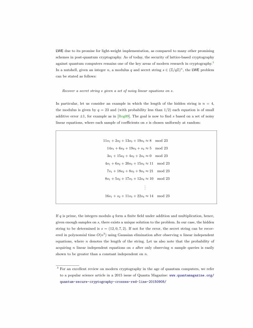
In particular, let us consider an example in which the length of the hidden string is n = 4,
the modulus is given by q = 23 and (with probability less than 1/2) each equation is of small
additive error ±1, for example as in [Reg09]. The goal is now to find s based on a set of noisy
linear equations, where each sample of coefficients on s is chosen uniformly at random:
11s1 + 2s2 + 13s3 + 19s4 ≈ 8 mod 23
14s1 + 6s2 + 19s3 + s4 ≈ 5 mod 23
3s1 + 15s2 + 4s3 + 2s4 ≈ 0 mod 23
4s1 + 6s2 + 20s3 + 15s4 ≈ 11 mod 23
7s1 + 18s2 + 8s3 + 9s4 ≈ 21 mod 23
8s1 + 5s2 + 17s3 + 12s4 ≈ 10 mod 23
...
16s1 + s2 + 11s3 + 22s4 ≈ 14 mod 23
If q is prime, the integers modulo q form a finite field under addition and multiplication, hence,
given enough samples on s, there exists a unique solution to the problem. In our case, the hidden
string to be determined is s = (12, 0, 7, 2). If not for the error, the secret string can be recov-
ered in polynomial time O(n3) using Gaussian elimination after observing n linear independent
equations, where n denotes the length of the string. Let us also note that the probability of
acquiring n linear independent equations on s after only observing n sample queries is easily
shown to be greater than a constant independent on n.
3 For an excellent review on modern cryptography in the age of quantum computers, we refer
to a popular science article in a 2015 issue of Quanta Magazine: www.quantamagazine.org/
quantum-secure-cryptography-crosses-red-line-20150908/
The difficulty in decoding noisy linear equations lies in the fact that the errors propagate dur-
ing the computation, hence amplify the uncertainty and ultimately lead to no information on
the actual secret string. As the best known algorithm for the LWE problem runs in time O(2n)
[BKW03], the problem is believed to be asymptotically intractible for classical computers. More-
over, due to the reduction in [Reg05], any breakthrough in LWE would also most likely imply
an algorithm for lattice-based problems.
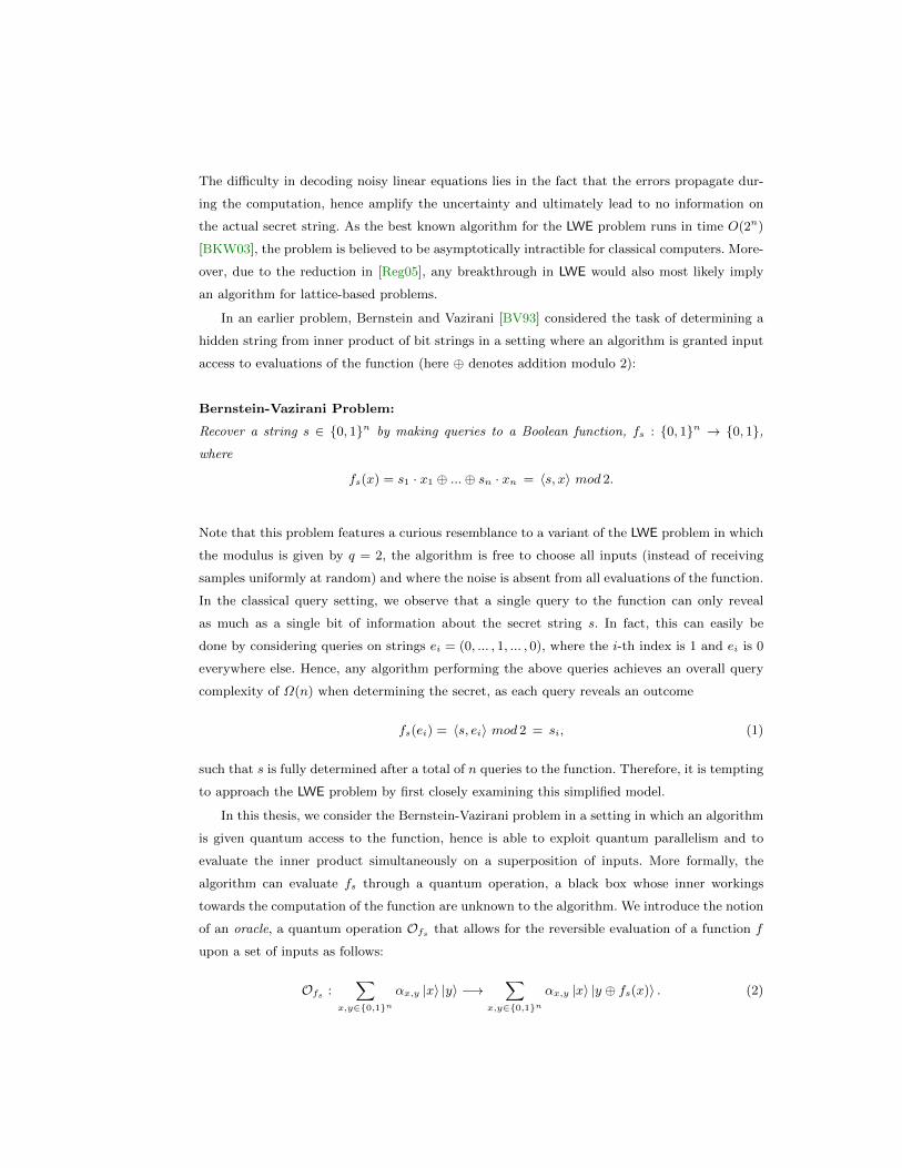
In an earlier problem, Bernstein and Vazirani [BV93] considered the task of determining a
hidden string from inner product of bit strings in a setting where an algorithm is granted input
access to evaluations of the function (here ⊕ denotes addition modulo 2):
Bernstein-Vazirani Problem:
Recover a string s ∈ 0, 1n by making queries to a Boolean function, fs : 0, 1n → 0, 1,
where
fs(x) = s1 · x1 ⊕ ...⊕ sn · xn = 〈s, x〉 mod 2.
Note that this problem features a curious resemblance to a variant of the LWE problem in which
the modulus is given by q = 2, the algorithm is free to choose all inputs (instead of receiving
samples uniformly at random) and where the noise is absent from all evaluations of the function.
In the classical query setting, we observe that a single query to the function can only reveal
as much as a single bit of information about the secret string s. In fact, this can easily be
done by considering queries on strings ei = (0, ... , 1, ... , 0), where the i-th index is 1 and ei is 0
everywhere else. Hence, any algorithm performing the above queries achieves an overall query
complexity of Ω(n) when determining the secret, as each query reveals an outcome
fs(ei) = 〈s, ei〉 mod 2 = si, (1)
such that s is fully determined after a total of n queries to the function. Therefore, it is tempting
to approach the LWE problem by first closely examining this simplified model.
In this thesis, we consider the Bernstein-Vazirani problem in a setting in which an algorithm
is given quantum access to the function, hence is able to exploit quantum parallelism and to
evaluate the inner product simultaneously on a superposition of inputs. More formally, the
algorithm can evaluate fs through a quantum operation, a black box whose inner workings
towards the computation of the function are unknown to the algorithm. We introduce the notion
of an oracle, a quantum operation Ofs that allows for the reversible evaluation of a function f
upon a set of inputs as follows:
Ofs :∑
x,y∈0,1nαx,y |x〉 |y〉 −→
∑x,y∈0,1n
αx,y |x〉 |y ⊕ fs(x)〉 . (2)
Remarkably, as Bernstein and Vazirani [BV93] showed, only a single oracle query to the the
function as in Eq.(2) is sufficient to determine the secret string. We generalize this model to
a group Z/qZ of arbitrary positive integers q under cyclic addition in a new learning problem
extension of the Bernstein-Vazirani algorithm and discuss its speed-up over classical algorithms.
Cross et al. [CSS14] have recently demonstrated a robustness of quantum learning for certain
classes of noise in which samples are also likely to be corrupted. While this setting is known to
cause most learning problems intractable for classical algorithms, the analogue using quantum
samples remains easy. Recently, Grilo et al. [GK17] independently considered a similar algorithm
for LWE, a special variant of our proposed extended Bernstein-Vazirani algorithm in which q is
prime. While this algorithm does not solve the LWE problem in its original formulation using
classical samples, it does however suggest further caution when allowing access to quantum
samples in any cryptographic application. Nevertheless, not even a quantum computer receiving
classical LWE samples, i.e. classical strings of noisy linear equations, seems to be able to challenge
the hardness of LWE [Reg09]. For this reason, LWE is still believed to be an excellent basis of
hardness in post-quantum cryptography.
While quantum superposition access is regularly shown to be a powerful model, it also pos-
sesses limitations. Our goal in this work is also to find such limitations in order to provide
quantum-secure encryption schemes, even in a setting in which an attacker has quantum access
to the encryption procedure. An essential building block for the construction of secure crypto-
graphic schemes is found in so-called pseudorandom functions, a family of keyed functions that
seem indistuinguishable from perfectly random functions to any adversary with limited compu-
tational recources. In fact, recent breakthroughs in quantum cryptography allow for quantum-
secure pseudorandom functions that are secure, even if an adversary is given the ability to
evaluate the function using quantum superpositions. Remarkably, as shown by Zhandry in 2012,
such constructions can be built using the classical sample hardness of LWE in the quantum world
[Zha12]:
If LWE with classical samples is hard for quantum computers, then there exist quantum-
secure pseudorandom functions.
As parallelism remains one of the key features of quantum algorithms, modern research is con-
cerned with exploitation of the nature of complex-valued amplitudes of quantum states in order
to cause them to interfere around the desired outputs through the use of quantum operations.
Only then, a final measurement of the state collapses the superposition into the desired outcome
with high probability. The following fact guarantees that quantum parallelism can be achieved
for all efficiently computable functions [NC10]:
Any classical efficiently computable function has an efficient circuit description, hence can also
be implemented efficiently using a quantum computer. Moreover, the quantum circuit for the
function consists entirely of unitary gates and can thus be evaluated on a superposition of inputs
due to the linearity of quantum mechanics.
A fundamental question arises immediately. Just how powerful is knowledge represented in
a quantum superposition evaluating a function on all of its inputs? This thesis is concerned
with both the limitation and exploitation of quantum parallelism in the context of modern
cryptography.
An important attack model in cryptanalysis is that of chosen-ciphertext attacks, a setting in
which an adversary exercises control over the encryption scheme, for example by manipulating
an honest party into generating both encryptions and decryptions of plaintexts or ciphertexts.
The security under chosen-ciphertext attacks is commonly formalized in an indistinguishability
game that takes place in two phases. In the pre-challenge phase, the adversary is allowed to
perform encryption and decryption queries. Then, upon a pair of two messages, the adversary
receives a challenge ciphertext, an encryption of one of the two messages at random, and proceeds
with another query phase. Typically, we grant encryption access during both phases, while for
decryption access, we differentiate between two important variants:
• (adaptive access) the adversary exercises full control and can perform informed decryption
queries both before and after the challenge phase begins, with the exception of the challenge
ciphertext itself.
• (non-adaptive access) the adversary exercises partial control and can only generate decryp-
tions prior to seeing the challenge ciphertext.
Oftentimes in cryptography jargon, the term lunchtime attack is adopted in order to highlight
a possible realistic setting for a non-adaptive attack model, whereas an adaptive attack corre-
sponds to full control over an honest party.
At STOC 2000, Katz and Yung [KY00] offered a complete characterization of classical se-
curity notions for private-key encryption. In the case of classical communication in a quantum
world, many of these security notions are still widely unexplored, and only few separation re-
sults have been successfully proven in recent years. At CRYPTO 2013, Boneh and Zhandry first
introduced the notion of adaptive quantum chosen-ciphertext security and proposed classical en-
cryption schemes for which such security can be achieved [BZ13]. An interesting open problem
concerns the class of non-adaptive quantum chosen-ciphertext attacks, a security notion in which
we allow adversaries to issue quantum superposition queries to encryption and non-adaptively
to decryption. In particular, it is unknown whether many of the standard encryption schemes
satisfy such a weaker notion of security.
3 Main Results
Let us now give an overview of the main contents provided in this thesis.
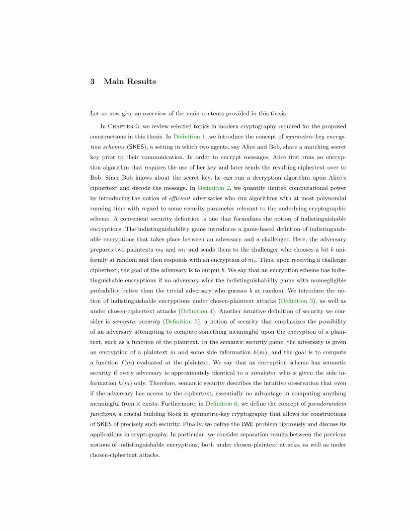
In Chapter 3, we review selected topics in modern cryptography required for the proposed
constructions in this thesis. In Definition 1, we introduce the concept of symmetric-key encryp-
tion schemes (SKES), a setting in which two agents, say Alice and Bob, share a matching secret
key prior to their communication. In order to encrypt messages, Alice first runs an encryp-
tion algorithm that requires the use of her key and later sends the resulting ciphertext over to
Bob. Since Bob knows about the secret key, he can run a decryption algorithm upon Alice’s
ciphertext and decode the message. In Definition 2, we quantify limited computational power
by introducing the notion of efficient adversaries who run algorithms with at most polynomial
running time with regard to some security parameter relevant to the underlying cryptographic
scheme. A convenient security definition is one that formalizes the notion of indistinguishable
encryptions. The indistinguishability game introduces a game-based defintion of indistinguish-
able encryptions that takes place between an adversary and a challenger. Here, the adversary
prepares two plaintexts m0 and m1 and sends them to the challenger who chooses a bit b uni-
formly at random and then responds with an encryption of mb. Thus, upon receiving a challenge
ciphertext, the goal of the adversary is to output b. We say that an encryption scheme has indis-
tinguishable encryptions if no adversary wins the indistinguishability game with nonnegligible
probability better than the trivial adversary who guesses b at random. We introduce the no-
tion of indistinguishable encryptions under chosen-plaintext attacks (Definition 3), as well as
under chosen-ciphertext attacks (Definition 4). Another intuitive definition of security we con-
sider is semantic security (Definition 5), a notion of security that emphasizes the possibility
of an adversary attempting to compute something meaningful upon the encryption of a plain-
text, such as a function of the plaintext. In the semantic security game, the adversary is given
an encryption of a plaintext m and some side information h(m), and the goal is to compute
a function f(m) evaluated at the plaintext. We say that an encryption scheme has semantic
security if every adversary is approximately identical to a simulator who is given the side in-
formation h(m) only. Therefore, semantic security describes the intuitive observation that even
if the adversary has access to the ciphertext, essentially no advantage in computing anything
meaningful from it exists. Furthermore, in Definition 6, we define the concept of pseudorandom
functions, a crucial building block in symmetric-key cryptography that allows for constructions
of SKES of precisely such security. Finally, we define the LWE problem rigorously and discuss its
applications in cryptography. In particular, we consider separation results between the previous
notions of indistinguishable encryptions, both under chosen-plaintext attacks, as well as under
chosen-ciphertext attacks.
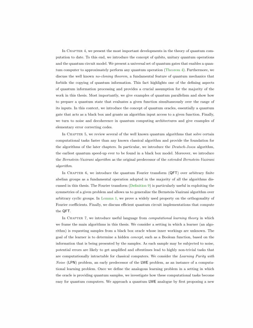
In Chapter 4, we present the most important developments in the theory of quantum com-
putation to date. To this end, we introduce the concept of qubits, unitary quantum operations
and the quantum circuit model. We present a universal set of quantum gates that enables a quan-
tum computer to approximately perform any quantum operation (Theorem 4). Furthermore, we
discuss the well known no-cloning theorem, a fundamental feature of quantum mechanics that
forbids the copying of quantum information. This fact highlights one of the defining aspects
of quantum information processing and provides a crucial assumption for the majority of the
work in this thesis. Most importantly, we give examples of quantum parallelism and show how
to prepare a quantum state that evaluates a given function simultaneously over the range of
its inputs. In this context, we introduce the concept of quantum oracles, essentially a quantum
gate that acts as a black box and grants an algorithm input access to a given function. Finally,
we turn to noise and decoherence in quantum computing architectures and give examples of
elementary error correcting codes.
In Chapter 5, we review several of the well known quantum algorithms that solve certain
computational tasks faster than any known classical algorithm and provide the foundation for
the algorithms of the later chapters. In particular, we introduce the Deutsch-Josza algorithm,
the earliest quantum speed-up ever to be found in a black box model. Moreover, we introduce
the Bernstein-Vazirani algorithm as the original predecessor of the extended Bernstein-Vazirani
algorithm.
In Chapter 6, we introduce the quantum Fourier transform (QFT) over arbitrary finite
abelian groups as a fundamental operation adopted in the majority of all the algorithms dis-
cussed in this thesis. The Fourier transform (Definition 9) is particularly useful in exploiting the
symmetries of a given problem and allows us to generalize the Bernstein-Vazirani algorithm over
arbitrary cyclic groups. In Lemma 1, we prove a widely used property on the orthogonality of
Fourier coefficients. Finally, we discuss efficient quantum circuit implementations that compute
the QFT.
In Chapter 7, we introduce useful language from computational learning theory in which
we frame the main algorithms in this thesis. We consider a setting in which a learner (an algo-
rithm) is requesting samples from a black box oracle whose inner workings are unknown. The
goal of the learner is to determine a hidden concept, such as a Boolean function, based on the
information that is being presented by the samples. As each sample may be subjected to noise,
potential errors are likely to get amplified and oftentimes lead to highly non-trivial tasks that
are computationally intractable for classical computers. We consider the Learning Parity with
Noise (LPN) problem, an early predecessor of the LWE problem, as an instance of a computa-
tional learning problem. Once we define the analogous learning problem in a setting in which
the oracle is providing quantum samples, we investigate how these computational tasks become
easy for quantum computers. We approach a quantum LWE analogue by first proposing a new
generalization of the Bernstein-Vazirani algorithm over an arbitrary cyclic group and show that
the secret string can be determined with high probability.
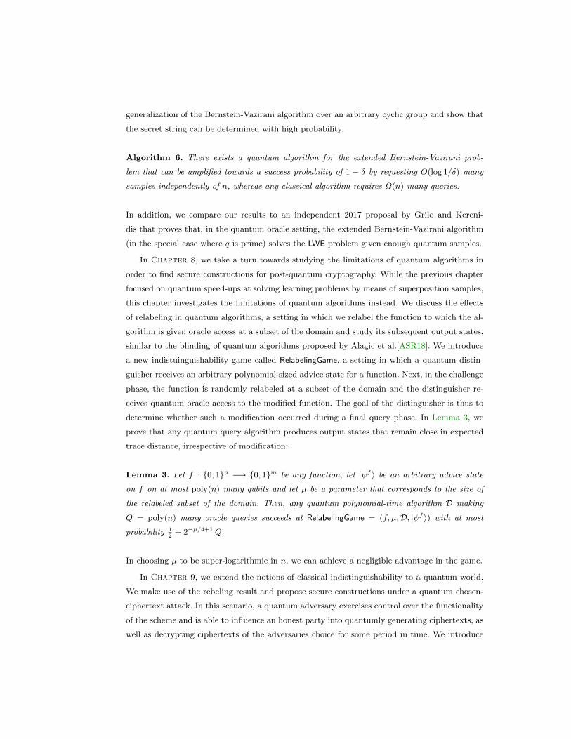
Algorithm 6. There exists a quantum algorithm for the extended Bernstein-Vazirani prob-
lem that can be amplified towards a success probability of 1 − δ by requesting O(log 1/δ) many
samples independently of n, whereas any classical algorithm requires Ω(n) many queries.
In addition, we compare our results to an independent 2017 proposal by Grilo and Kereni-
dis that proves that, in the quantum oracle setting, the extended Bernstein-Vazirani algorithm
(in the special case where q is prime) solves the LWE problem given enough quantum samples.
In Chapter 8, we take a turn towards studying the limitations of quantum algorithms in
order to find secure constructions for post-quantum cryptography. While the previous chapter
focused on quantum speed-ups at solving learning problems by means of superposition samples,
this chapter investigates the limitations of quantum algorithms instead. We discuss the effects
of relabeling in quantum algorithms, a setting in which we relabel the function to which the al-
gorithm is given oracle access at a subset of the domain and study its subsequent output states,
similar to the blinding of quantum algorithms proposed by Alagic et al.[ASR18]. We introduce
a new indistuinguishability game called RelabelingGame, a setting in which a quantum distin-
guisher receives an arbitrary polynomial-sized advice state for a function. Next, in the challenge
phase, the function is randomly relabeled at a subset of the domain and the distinguisher re-
ceives quantum oracle access to the modified function. The goal of the distinguisher is thus to
determine whether such a modification occurred during a final query phase. In Lemma 3, we
prove that any quantum query algorithm produces output states that remain close in expected
trace distance, irrespective of modification:
Lemma 3. Let f : 0, 1n −→ 0, 1m be any function, let |ψf 〉 be an arbitrary advice state
on f on at most poly(n) many qubits and let µ be a parameter that corresponds to the size of
the relabeled subset of the domain. Then, any quantum polynomial-time algorithm D making
Q = poly(n) many oracle queries succeeds at RelabelingGame = (f, µ,D, |ψf 〉) with at most
probability 12
+ 2−µ/4+1Q.
In choosing µ to be super-logarithmic in n, we can achieve a negligible advantage in the game.
In Chapter 9, we extend the notions of classical indistinguishability to a quantum world.
We make use of the rebeling result and propose secure constructions under a quantum chosen-
ciphertext attack. In this scenario, a quantum adversary exercises control over the functionality
of the scheme and is able to influence an honest party into quantumly generating ciphertexts, as
well as decrypting ciphertexts of the adversaries choice for some period in time. We introduce
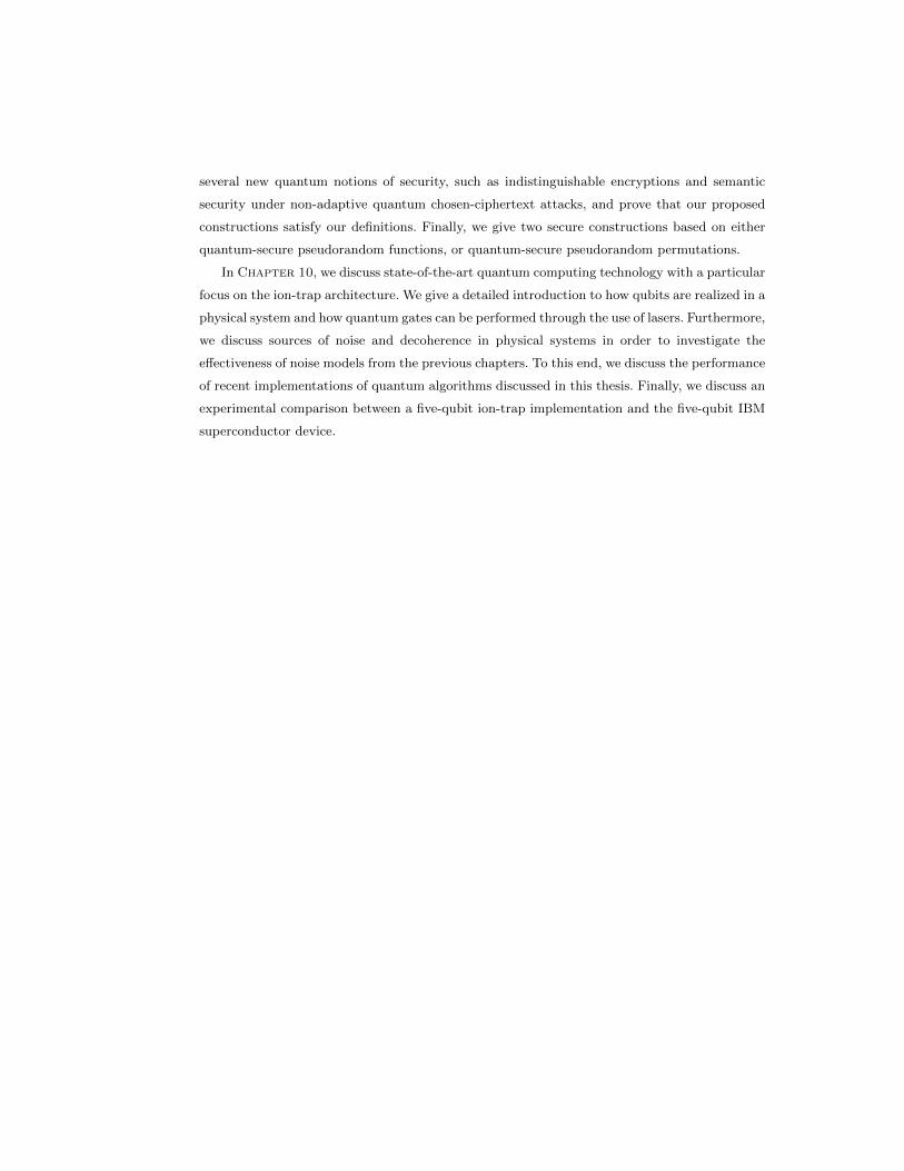
several new quantum notions of security, such as indistinguishable encryptions and semantic
security under non-adaptive quantum chosen-ciphertext attacks, and prove that our proposed
constructions satisfy our definitions. Finally, we give two secure constructions based on either
quantum-secure pseudorandom functions, or quantum-secure pseudorandom permutations.
In Chapter 10, we discuss state-of-the-art quantum computing technology with a particular
focus on the ion-trap architecture. We give a detailed introduction to how qubits are realized in a
physical system and how quantum gates can be performed through the use of lasers. Furthermore,
we discuss sources of noise and decoherence in physical systems in order to investigate the
effectiveness of noise models from the previous chapters. To this end, we discuss the performance
of recent implementations of quantum algorithms discussed in this thesis. Finally, we discuss an
experimental comparison between a five-qubit ion-trap implementation and the five-qubit IBM
superconductor device.
4 Cryptography
The history of cryptography dates back to over two millenia. Ever since the birth of civilization
and the invention of writing, people required ways of transmitting secret messages using ciphers,
intended to be read only by the receiver and yet difficult to decode for others. Since the 1970s,
cryptography amounted to a well-established scientific discipline by henceforth adopting a rigor-
ous mathematical foundation. This crucial change marks the beginning of modern cryptography.
Many of the popular encryption schemes still in use today, such as the RSA encryption scheme,
were already developed in the early years of modern cryptography. Typically, it is the hardness
of certain computational problems that serves as a foundation for security. For example, as in
the case of RSA, the security of the encryption scheme is related to the hardness of factor-
ing large integers. In other words, we believe a scheme is secure, if no efficient adversary with
limited computational recources is capable of breaking the scheme. Peter Shor’s discovery of an
efficient quantum algorithm for the factoring of integers marked the beginning of an entirely new
era of cryptography, a so-called post-quantum cryptography. It is from here on, that the search
for quantum-secure cryptography began. In the following sections, we provide an overview of
selected topics in modern cryptography required for the main results in this thesis.
4.1 Preliminaries
Let us first introduce some necessary notation and formalism from theoretical computer science
and cryptography. For additional reading, we refer to [KL15].
For bit strings x ∈ 0, 1n of arbitrary length n = |x|, we associate a product space 0, 1∗
containing all such strings of finite length. A function ε : N→ R is called negligible if, for every
polynomial p, there exists an integer N such that for all n > N , it holds that: ε(n) < 1p(n)
.
Typically, we adopt negligible functions in the context of a success probability that decreases
to an inverse-superpolynomial rate, hence cannot be amplified to a constant by a polynomial
amount of repetitions. An algorithm is a sequence of (possibly nondeterministic) operations
that terminates after a finite amount of steps upon any given input, say x ∈ 0, 1∗. We say
an algorithm is efficient if it has polynomial running time with respect to a size parameter of
a given computational problem, i.e. if there exists a polynomial p(x) such that, for any input
x ∈ 0, 1∗, the computation of A(x) terminates after at most p(|x|) steps. A probabilistic poly-
nomial time (PPT) algorithm is a procedure with an additional random tape (such as a random
number generator) that results in efficient, yet possibly nondeterministic, computations. We
adopt the popular unary convention of representing the seed of efficient randomized algorithms
by 1n = 11...1, highlighting a polynomial dependence with respect to the length of the input,
contrary to a polylog dependence in the general case where dlog2(n)e bits are needed to specify
the length of a given input (here, d·e denotes the ceiling function). With x $←−X, we denote a
procedure an outcome x is sampled uniformly at random from a finite set X. If D is a proba-
bility distribution, we denote the sampling of an outcome according to D by using the notation
x← D. Upon finite sets X and Y , we define the corresponding (finite) set of all possible func-
tions from X to Y as F : X → Y. An oracle is a black box machine O that assists a given
algorithm with a particular computational task at unit cost, for example in an evaluation of an
unknown function upon a given input or the sampling from an unknown probability distribution.
Typically, if A is an algorithm, we denote oracle access to O using the notation AO. Finally,
throughout this thesis, we employ the usual asymptotic O-notation denoting an upper bound,
where for a given function g(n), we define O(g(n)) = f(n) : ∃c ∈ R, ∃n ∈ N such that 0 ≤
f(n) ≤ c g(n), ∀n ≥ n0. Similarly, we denote an asymptotic lower-bound Ω(g(n)) as the set of
functions Ω(g(n)) = f(n) : ∃c ∈ R,∃n ∈ N such that 0 ≤ c g(n) ≤ f(n), ∀n ≥ n0.
4.2 Symmetric-Key Cryptography
Symmetric-key cryptography concerns the scenario in which two agents, say Alice and Bob,
share a mutual secret key k prior to their communication and want to send messages to each
other. In order to encrypt messages, Alice first chooses a message m and runs an encryption
algorithm Enck(m) that requires the use of her key and later sends the resulting ciphertext c
over to Bob. Since Bob knows about the secret key, he can run a decryption algorithm Deck(c)
upon Alice’s ciphertext and decode the message. In general, we consider randomized encryption
in order to avoid replay attacks, while only requiring decryption to be deterministic.
Definition 1. A symmetric-key encryption scheme (SKES) Π = (KeyGen,Enc,Dec) is a triple
of PPT algorithms on a finite key space K, message space M and ciphertext space C, where
KeyGen : N → K, Enc : K ×M → C, Dec : K × C → M and, for a security parameter n, we
require:
1. (key generation) KeyGen: on input 1n, generate a key k ← KeyGen(1n);
2. (encryption) Enck: on message m ∈M, output a ciphertext Enck(m);
3. (decryption) Deck: on cipher c ∈ C, output a message Deck(c);
4. (correctness) (Deck Enck)(m) = m.
In order for communication under a given symmetric-key encryption scheme to be secure against
eavesdroppers, we require that, without knowledge of the secret key, any ciphertext must look
sufficiently random and reveal little to no information about the actual message.
In the next section, we provide several widely used notions of security for symmetric-key en-
cryption. For further reading, we refer to [KL15].
4.3 Security Notions
Computational Security Due to the well known P-NP problem, i.e. the seeming impossibil-
ity of finding efficient algorithms for certain hard computational problems, and the fact that we
consider adversaries who operate probabilistically, an important notion of security is provided
by computational security based on the following principle:
A successful cipher must be practically secure against adversaries with limited computational
recources.
This brings us to the following definition of computational security:
Definition 2 (Computational Security). A scheme Π = (KeyGen,Enc,Dec) is computa-
tionally (or asymptotically) secure if every PPT adversary succeeds at breaking Π with at most
negligible probability with respect to the security parameter of Π.
Since a negligible success probability is smaller than the inverse of any polynomial, no efficient
algorithm is capable of amplifying the success probability, i.e. capable of breaking the encryption
scheme by sheer repetition. Therefore, we regard any algorithm that breaks a particular scheme
with at most negligible probability as not significant.
Computational Indistinguishability. Another important notion of security for a given
symmetric-key encryption scheme is indistinguishability of encryptions, in particular under a
chosen-plaintext attack. In this model, an adversary has partial control over the encryption
procedure and can generate encryptions of arbitrary messages. This attack corresponds to a
scenario in which an attacker is able to influence an honest party into generating ciphertexts of
the adversaries choice, thus potentially resulting in an advantage at decoding other ciphers of
interest. In the following, we specify this model in a security game between an adversary and a
challenger:
Definition 3 (IND-CPA).
Let Π = (KeyGen,Enc,Dec) be a symmetric-key encryption scheme and consider the IndGame
between a PPT adversary and challenger, defined as follows:
1. (initial phase) the challenger chooses a key k ← KeyGen(1n) and bit b $←−0, 1;
2. (pre-challenge phase) as part of a learning phase, the adversary is given access to an en-
cryption oracle Enck in order to generate encryptions. Upon each choice of message m, the
adversary receives a ciphertext c ← Enck(m). Finally, the adversary chooses two messages
m0 and m1, and sends them to the challenger.
3. (challenge phase) the challenger replies with Enck(mb) and the adversary continues to have
oracle access to Enck;
4. (resolution) the adversary outputs a bit b′ and wins the game if b′ = b.
We say that Π has indistinguishable encryptions under a chosen-plaintext attack (or is IND-CPA-
secure) if, for every PPT A, there exists a negligible function ε(n) such that:
Pr[A wins IndGame] ≤ 1/2 + ε(n).
An even stronger notion of security for a given symmetric-key encryption scheme is security
under chosen-ciphertext attacks. In this variant of the IndGame, an adversary not only exercises
control over the encryption scheme as before, but can also non-adaptively decrypt messages
unrelated to a ciphertext of interest (as highlighted in the pre-challenge and challenge phase).
Therefore, such an attack corresponds to a scenario in which an attacker is able to exercise
control over an honest party into generating ciphertexts, as well as decrypting ciphertexts of the
adversaries choice for some period in time. In the following, we specify this model in another
security game between an adversary and a challenger:
Definition 4 (IND-CCA1).
Let Π = (KeyGen,Enc,Dec) be a symmetric-key encryption scheme and consider the IndGame
between a PPT adversary and challenger, defined as follows:
1. (initial phase) the challenger chooses a key k ← KeyGen(1n) and bit b $←−0, 1;
2. (pre-challenge phase) as part of a learning phase, the adversary is given access to both an
encryption oracle Enck and decryption oracle Deck. Upon each choice of message m, the
adversary receives a ciphertext Enck(m) and, upon each ciphertext c, the adversary receives
a plaintext Deck(c). Finally, the adversary chooses two messages m0 and m1, and sends
them to the challenger.
3. (challenge phase) the challenger replies with Enck(mb) and the adversary continues to have
oracle access to Enck only;
4. (resolution) the adversary outputs a bit b′ and wins the game if b′ = b.
We say that Π has indistinguishable encryptions under a chosen-ciphertext attack (or is IND-CCA1-
secure) if, for every PPT A, there exists a negligible function ε(n) such that:
Pr[A wins IndGame] ≤ 1/2 + ε(n).
Finally, we can additionally extend the previous notion of IND-CCA1 security by also granting
the adversary adaptive decryption access after the challenge phase. This model corresponds to
IND-CCA2 security, a variant in which the adversary exercises full control over the encryption
scheme, both before and after the challenge phase. Remarkably, there exist classical symmetric-
key encryption schemes that satisfy each of the security definitions provided in this chapter.
A major contribution of this thesis is to provide constructions that satisfy these notions, even
in a setting in which the adversary is granted quantum superposition access, again both to
the encryption and decryption procedure. In the next section, we introduce important tools to
realize such cryptographic schemes.
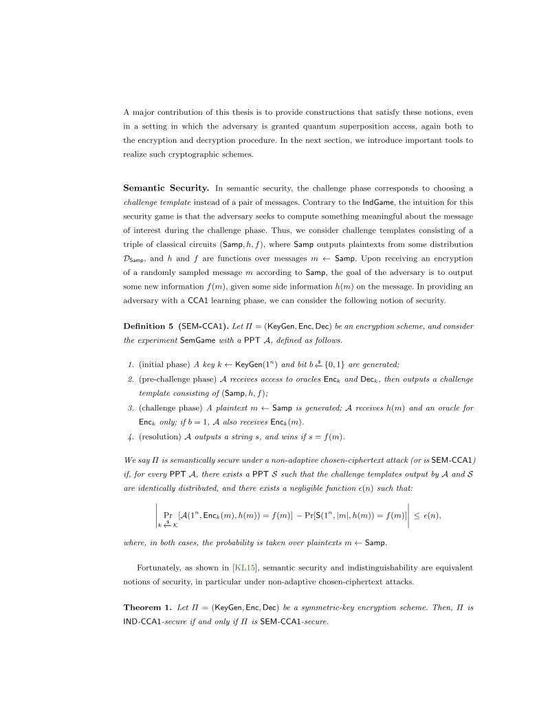
Semantic Security. In semantic security, the challenge phase corresponds to choosing a
challenge template instead of a pair of messages. Contrary to the IndGame, the intuition for this
security game is that the adversary seeks to compute something meaningful about the message
of interest during the challenge phase. Thus, we consider challenge templates consisting of a
triple of classical circuits (Samp, h, f), where Samp outputs plaintexts from some distribution
DSamp, and h and f are functions over messages m ← Samp. Upon receiving an encryption
of a randomly sampled message m according to Samp, the goal of the adversary is to output
some new information f(m), given some side information h(m) on the message. In providing an
adversary with a CCA1 learning phase, we can consider the following notion of security.
Definition 5 (SEM-CCA1). Let Π = (KeyGen,Enc,Dec) be an encryption scheme, and consider
the experiment SemGame with a PPT A, defined as follows.
1. (initial phase) A key k ← KeyGen(1n) and bit b $←−0, 1 are generated;
2. (pre-challenge phase) A receives access to oracles Enck and Deck, then outputs a challenge
template consisting of (Samp, h, f);
3. (challenge phase) A plaintext m ← Samp is generated; A receives h(m) and an oracle for
Enck only; if b = 1, A also receives Enck(m).
4. (resolution) A outputs a string s, and wins if s = f(m).
We say Π is semantically secure under a non-adaptive chosen-ciphertext attack (or is SEM-CCA1)
if, for every PPT A, there exists a PPT S such that the challenge templates output by A and S
are identically distributed, and there exists a negligible function ε(n) such that:∣∣∣∣∣ Prk
$←−K[A(1n,Enck(m), h(m)) = f(m)] − Pr[S(1n, |m|, h(m)) = f(m)]
∣∣∣∣∣ ≤ ε(n),
where, in both cases, the probability is taken over plaintexts m← Samp.
Fortunately, as shown in [KL15], semantic security and indistinguishability are equivalent
notions of security, in particular under non-adaptive chosen-ciphertext attacks.
Theorem 1. Let Π = (KeyGen,Enc,Dec) be a symmetric-key encryption scheme. Then, Π is
IND-CCA1-secure if and only if Π is SEM-CCA1-secure.
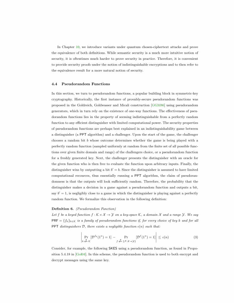
In Chapter 10, we introduce variants under quantum chosen-ciphertext attacks and prove
the equivalence of both definitions. While semantic security is a much more intuitive notion of
security, it is oftentimes much harder to prove security in practice. Therefore, it is convenient
to provide security proofs under the notion of indistinguishable encryptions and to then refer to
the equivalence result for a more natural notion of security.
4.4 Pseudorandom Functions
In this section, we turn to pseudorandom functions, a popular building block in symmetric-key
cryptography. Historically, the first instance of provably-secure pseudorandom functions was
proposed in the Goldreich, Goldwasser and Micali construction [GGM86] using pseudorandom
generators, which in turn rely on the existence of one-way functions. The effectiveness of pseu-
dorandom functions lies in the property of seeming indistinguishable from a perfectly random
function to any efficient distinguisher with limited computational power. The security properties
of pseudorandom functions are perhaps best explained in an indistinguishability game between
a distinguisher (a PPT algorithm) and a challenger. Upon the start of the game, the challenger
chooses a random bit b whose outcome determines whether the game is being played with a
perfectly random function (sampled uniformly at random from the finite set of all possible func-
tions over given finite domain and range) of the challengers choice, or a pseudorandom function
for a freshly generated key. Next, the challenger presents the distinguisher with an oracle for
the given function who is then free to evaluate the function upon arbitrary inputs. Finally, the
distinguisher wins by outputting a bit b′ = b. Since the distinguisher is assumed to have limited
computational recources, thus essentially running a PPT algorithm, the claim of pseudoran-
domness is that the outputs will look sufficiently random. Therefore, the probability that the
distinguisher makes a decision in a game against a pseudorandom function and outputs a bit,
say b′ = 1, is negligibly close to a game in which the distinguisher is playing against a perfectly
random function. We formalize this observation in the following definition:
Definition 6. (Pseudorandom Function)
Let f be a keyed function f : K×X → Y on a key-space K, a domain X and a range Y. We say
PRF = fkk∈K is a family of pseudorandom functions if, for every choice of key k and for all
PPT distinguishers D, there exists a negligible function ε(n) such that:∣∣∣∣∣ Prk
$←−K[Dfk (1n) = 1] − Pr
f$←− F:X→Y
[Df (1n) = 1]
∣∣∣∣∣ ≤ ε(n) (3)
Consider, for example, the following SKES using a pseudorandom function, as found in Propo-
sition 5.4.18 in [Gol04]. In this scheme, the pseudorandom function is used to both encrypt and
decrypt messages using the same key.
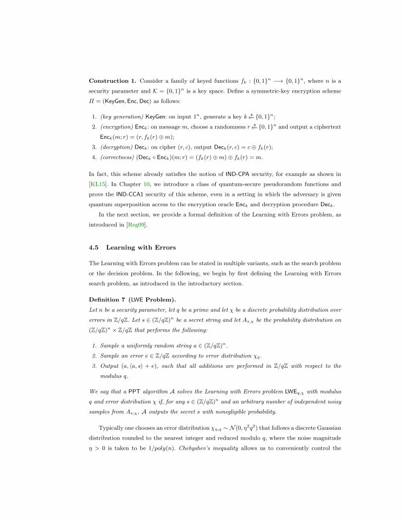
Construction 1. Consider a family of keyed functions fk : 0, 1n −→ 0, 1n, where n is a
security parameter and K = 0, 1n is a key space. Define a symmetric-key encryption scheme
Π = (KeyGen,Enc,Dec) as follows:
1. (key generation) KeyGen: on input 1n, generate a key k $←−0, 1n;
2. (encryption) Enck: on message m, choose a randomness r $←−0, 1n and output a ciphertext
Enck(m; r) = (r, fk(r)⊕m);
3. (decryption) Deck: on cipher (r, c), output Deck(r, c) = c⊕ fk(r);
4. (correctness) (Deck Enck)(m; r) = (fk(r)⊕m)⊕ fk(r) = m.
In fact, this scheme already satisfies the notion of IND-CPA security, for example as shown in
[KL15]. In Chapter 10, we introduce a class of quantum-secure pseudorandom functions and
prove the IND-CCA1 security of this scheme, even in a setting in which the adversary is given
quantum superposition access to the encryption oracle Enck and decryption procedure Deck.
In the next section, we provide a formal definition of the Learning with Errors problem, as
introduced in [Reg09].
4.5 Learning with Errors
The Learning with Errors problem can be stated in multiple variants, such as the search problem
or the decision problem. In the following, we begin by first defining the Learning with Errors
search problem, as introduced in the introductory section.
Definition 7 (LWE Problem).
Let n be a security parameter, let q be a prime and let χ be a discrete probability distribution over
errors in Z/qZ. Let s ∈ (Z/qZ)n be a secret string and let As,χ be the probability distribution on
(Z/qZ)n × Z/qZ that performs the following:
1. Sample a uniformly random string a ∈ (Z/qZ)n.
2. Sample an error e ∈ Z/qZ according to error distribution χq.
3. Output (a, 〈a, s〉 + e), such that all additions are performed in Z/qZ with respect to the
modulus q.
We say that a PPT algorithm A solves the Learning with Errors problem LWEq,χ with modulus
q and error distribution χ if, for any s ∈ (Z/qZ)n and an arbitrary number of independent noisy
samples from As,χ, A outputs the secret s with nonegligible probability.
Typically one chooses an error distribution χη,q ∼ N (0, η2q2) that follows a discrete Gaussian
distribution rounded to the nearest integer and reduced modulo q, where the noise magnitude
η > 0 is taken to be 1/poly(n). Chebyshev’s inequality allows us to conveniently control the
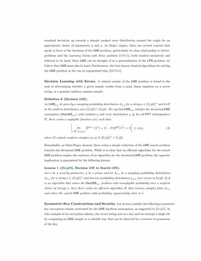
standard deviation ηq towards a sharply peaked error distribution around the origin for an
appriopriate choice of parameters η and q. As Regev argues, there are several reasons that
speak in favor of the hardness of the LWE problem, particularly its close relationship to lattice-
problems and the Learning Parity with Noise problem [CSS14], both studied extensively and
believed to be hard. Since LWE can be thought of as a generalization of the LPN problem, we
believe that LWE must also be hard. Furthermore, the best known classical algorithms for solving
the LWE problem so far run in exponential time [BKW03].
Decision Learning with Errors. A related variant of the LWE problem is found in the
task of determining whether a given sample results from a noisy linear equation on a secret
string, or a genuine uniform random sample.
Definition 8 (Decision LWE).
Let LWEq,χ be given by a sampling probability distribution As,χ for a string s ∈ (Z/qZ)n and let O
be the uniform distribution over (Z/qZ)n×Z/qZ. We say that LWEq,χ satisfies the decisional LWE
assumption (DecLWEq,χ) with modulus q and error distribution χ if, for all PPT distinguishers
D, there exists a negligible function ε(n) such that:∣∣∣∣∣ Prs
$←− (Z/qZ)n[DAs,χ(1n) = 1] − Pr[DO(1n) = 1]
∣∣∣∣∣ ≤ ε(n), (4)
where O outputs uniform samples (a, u) $←− (Z/qZ)n × Z/qZ.
Remarkably, as Oded Regev showed, there exists a simple reduction of the LWE search problem
towards the decisional LWE problem. While it is clear that an efficient algorithm for the search
LWE problem implies the existence of an algorithm for the decisional LWE problem, the opposite
implication is guaranteed by the following lemma:
Lemma 1 ([Reg09], Decision LWE to Search LWE).
Let n be a security parameter, q be a prime and let As,χ be a sampling probability distribution
As,χ for a string s ∈ (Z/qZ)n and discrete probability distribution χq,η over errors in Z/qZ. If A
is an algorithm that solves the DecLWEq,χ problem with nonegligible probability over a uniform
choice of strings s, then there exists an efficient algorithm A′ that receives samples from As,χ
and solves the search LWE problem with probability exponentially close to 1.
Symmetric-Key Constructions and Security. Let us now consider the following symmetric-
key encryption scheme motivated by the LWE hardness assumption, as suggested in [Reg05]. In
this example of an encryption scheme, the secret string acts as a key and we encrypt a single bit
by computing an LWE sample in a suitable way that can be detected by a receiver in possession
of the key.
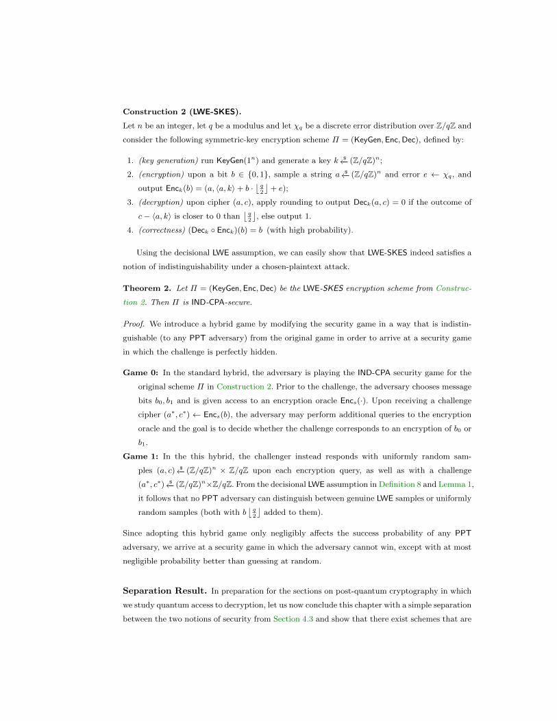
Construction 2 (LWE-SKES).
Let n be an integer, let q be a modulus and let χq be a discrete error distribution over Z/qZ and
consider the following symmetric-key encryption scheme Π = (KeyGen,Enc,Dec), defined by:
1. (key generation) run KeyGen(1n) and generate a key k $←− (Z/qZ)n;
2. (encryption) upon a bit b ∈ 0, 1, sample a string a $←− (Z/qZ)n and error e ← χq, and
output Enck(b) = (a, 〈a, k〉+ b ·⌊q2
⌋+ e);
3. (decryption) upon cipher (a, c), apply rounding to output Deck(a, c) = 0 if the outcome of
c− 〈a, k〉 is closer to 0 than⌊q2
⌋, else output 1.
4. (correctness) (Deck Enck)(b) = b (with high probability).
Using the decisional LWE assumption, we can easily show that LWE-SKES indeed satisfies a
notion of indistinguishability under a chosen-plaintext attack.
Theorem 2. Let Π = (KeyGen,Enc,Dec) be the LWE-SKES encryption scheme from Construc-
tion 2. Then Π is IND-CPA-secure.
Proof. We introduce a hybrid game by modifying the security game in a way that is indistin-
guishable (to any PPT adversary) from the original game in order to arrive at a security game
in which the challenge is perfectly hidden.
Game 0: In the standard hybrid, the adversary is playing the IND-CPA security game for the
original scheme Π in Construction 2. Prior to the challenge, the adversary chooses message
bits b0, b1 and is given access to an encryption oracle Encs(·). Upon receiving a challenge
cipher (a∗, c∗) ← Encs(b), the adversary may perform additional queries to the encryption
oracle and the goal is to decide whether the challenge corresponds to an encryption of b0 or
b1.
Game 1: In the this hybrid, the challenger instead responds with uniformly random sam-
ples (a, c) $←− (Z/qZ)n × Z/qZ upon each encryption query, as well as with a challenge
(a∗, c∗) $←− (Z/qZ)n×Z/qZ. From the decisional LWE assumption in Definition 8 and Lemma 1,
it follows that no PPT adversary can distinguish between genuine LWE samples or uniformly
random samples (both with b⌊q2
⌋added to them).
Since adopting this hybrid game only negligibly affects the success probability of any PPT
adversary, we arrive at a security game in which the adversary cannot win, except with at most
negligible probability better than guessing at random.
Separation Result. In preparation for the sections on post-quantum cryptography in which
we study quantum access to decryption, let us now conclude this chapter with a simple separation
between the two notions of security from Section 4.3 and show that there exist schemes that are
IND-CPA-secure but not IND-CCA1-secure. Using the LWE-SKES scheme, we can easily prove
such a separation. The intuition is that decryption oracle access in this scheme allows the
adversary to evaluate the noisy inner product upon arbitrary inputs. As a result, the adversary
can determine parts of the secret key using only a few queries to its decryption oracle.
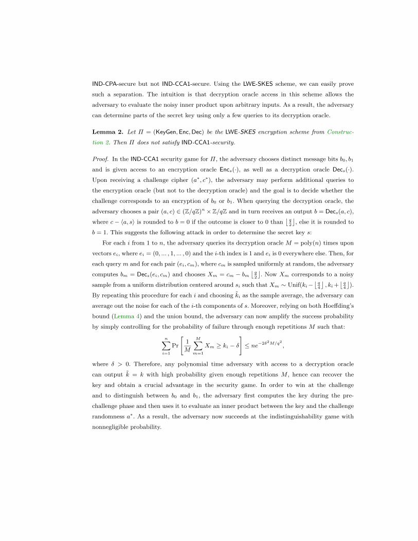
Lemma 2. Let Π = (KeyGen,Enc,Dec) be the LWE-SKES encryption scheme from Construc-
tion 2. Then Π does not satisfy IND-CCA1-security.
Proof. In the IND-CCA1 security game for Π, the adversary chooses distinct message bits b0, b1
and is given access to an encryption oracle Encs(·), as well as a decryption oracle Decs(·).
Upon receiving a challenge cipher (a∗, c∗), the adversary may perform additional queries to
the encryption oracle (but not to the decryption oracle) and the goal is to decide whether the
challenge corresponds to an encryption of b0 or b1. When querying the decryption oracle, the
adversary chooses a pair (a, c) ∈ (Z/qZ)n ×Z/qZ and in turn receives an output b = Decs(a, c),
where c− 〈a, s〉 is rounded to b = 0 if the outcome is closer to 0 than⌊q2
⌋, else it is rounded to
b = 1. This suggests the following attack in order to determine the secret key s:
For each i from 1 to n, the adversary queries its decryption oracle M = poly(n) times upon
vectors ei, where ei = (0, ... , 1, ... , 0) and the i-th index is 1 and ei is 0 everywhere else. Then, for
each query m and for each pair (ei, cm), where cm is sampled uniformly at random, the adversary
computes bm = Decs(ei, cm) and chooses Xm = cm − bm⌊q2
⌋. Now Xm corresponds to a noisy
sample from a uniform distribution centered around si such that Xm ∼ Unif(ki−⌊q4
⌋, ki+
⌊q4
⌋).
By repeating this procedure for each i and choosing ki as the sample average, the adversary can
average out the noise for each of the i-th components of s. Moreover, relying on both Hoeffding’s
bound (Lemma 4) and the union bound, the adversary can now amplify the success probability
by simply controlling for the probability of failure through enough repetitions M such that:
n∑i=1
Pr
[1
M
M∑m=1
Xm ≥ ki − δ
]≤ ne−2δ2M/q2 ,
where δ > 0. Therefore, any polynomial time adversary with access to a decryption oracle
can output k = k with high probability given enough repetitions M , hence can recover the
key and obtain a crucial advantage in the security game. In order to win at the challenge
and to distinguish between b0 and b1, the adversary first computes the key during the pre-
challenge phase and then uses it to evaluate an inner product between the key and the challenge
randomness a∗. As a result, the adversary now succeeds at the indistinguishability game with
nonnegligible probability.
5 Quantum Computation
Quantum information processing is concerned with the storage and manipulation of information
in a quantum system. The fundamental unit of information is the qubit, a quantum two-level
system of states |0〉 and |1〉. Fortunately, nature presents us with many ways of realizing a qubit
in a physical system. Typical representations of a qubit are found in the two spin 1/2 states of
a particle, the vertical or horizontal polarization of a photon or simply a ground and excited
state in the energy spectrum of an atom. In this chapter, we give a brief overview of the most
important concepts in the theory of quantum computing to date. For further reading, we refer
to [NC10]. Finally, with regard to the physical realization of quantum computers, we refer to
Chapter 11.
5.1 Formalism
A quantum system is a Hilbert space H, a complex vector space together with an inner product
〈·|·〉. A qubit is a quantum system |ψ〉 of mutually orthogonal basis states |0〉 and |1〉, given by
a normalized state vector of amplitudes |α|2 + |β|2 = 1, where
|ψ〉 = α |0〉+ β |1〉 . (5)
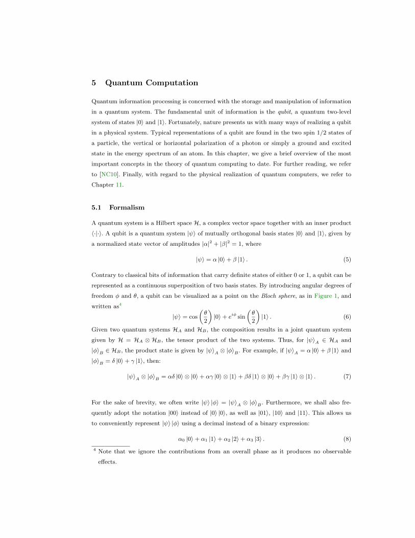
Contrary to classical bits of information that carry definite states of either 0 or 1, a qubit can be
represented as a continuous superposition of two basis states. By introducing angular degrees of
freedom φ and θ, a qubit can be visualized as a point on the Bloch sphere, as in Figure 1, and
written as4
|ψ〉 = cos
(θ
2
)|0〉+ eiφ sin
(θ
2
)|1〉 . (6)
Given two quantum systems HA and HB , the composition results in a joint quantum system
given by H = HA ⊗ HB , the tensor product of the two systems. Thus, for |ψ〉A ∈ HA and
|φ〉B ∈ HB , the product state is given by |ψ〉A ⊗ |φ〉B . For example, if |ψ〉A = α |0〉+ β |1〉 and
|φ〉B = δ |0〉+ γ |1〉, then:
|ψ〉A ⊗ |φ〉B = αδ |0〉 ⊗ |0〉+ αγ |0〉 ⊗ |1〉+ βδ |1〉 ⊗ |0〉+ βγ |1〉 ⊗ |1〉 . (7)
For the sake of brevity, we often write |ψ〉 |φ〉 = |ψ〉A ⊗ |φ〉B . Furthermore, we shall also fre-
quently adopt the notation |00〉 instead of |0〉 |0〉, as well as |01〉, |10〉 and |11〉. This allows us
to conveniently represent |ψ〉 |φ〉 using a decimal instead of a binary expression:
α0 |0〉+ α1 |1〉+ α2 |2〉+ α3 |3〉 . (8)
4 Note that we ignore the contributions from an overall phase as it produces no observable
effects.
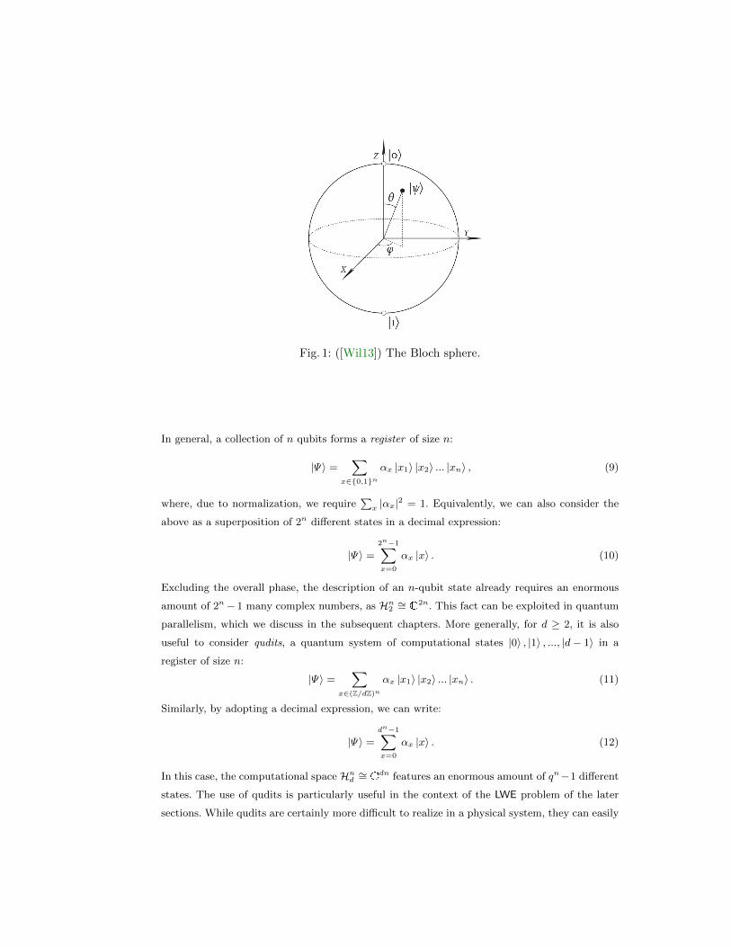
Fig. 1: ([Wil13]) The Bloch sphere.
In general, a collection of n qubits forms a register of size n:
|Ψ〉 =∑
x∈0,1nαx |x1〉 |x2〉 ... |xn〉 , (9)
where, due to normalization, we require∑x |αx|
2 = 1. Equivalently, we can also consider the
above as a superposition of 2n different states in a decimal expression:
|Ψ〉 =
2n−1∑x=0
αx |x〉 . (10)
Excluding the overall phase, the description of an n-qubit state already requires an enormous
amount of 2n− 1 many complex numbers, as Hn2 ∼= C2n. This fact can be exploited in quantum
parallelism, which we discuss in the subsequent chapters. More generally, for d ≥ 2, it is also
useful to consider qudits, a quantum system of computational states |0〉 , |1〉 , ..., |d− 1〉 in a
register of size n:
|Ψ〉 =∑
x∈(Z/dZ)nαx |x1〉 |x2〉 ... |xn〉 . (11)
Similarly, by adopting a decimal expression, we can write:
|Ψ〉 =
dn−1∑x=0
αx |x〉 . (12)
In this case, the computational space Hnd ∼= Cdn features an enormous amount of qn−1 different
states. The use of qudits is particularly useful in the context of the LWE problem of the later
sections. While qudits are certainly more difficult to realize in a physical system, they can easily
be emulated with qubits by using a block encoding in which each qudit is packed into dlog2(d)e
many qubits.
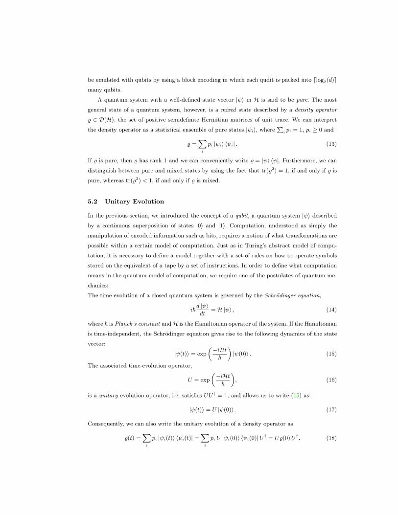
A quantum system with a well-defined state vector |ψ〉 in H is said to be pure. The most
general state of a quantum system, however, is a mixed state described by a density operator
% ∈ D(H), the set of positive semidefinite Hermitian matrices of unit trace. We can interpret
the density operator as a statistical ensemble of pure states |ψi〉, where∑i pi = 1, pi ≥ 0 and
% =∑i
pi |ψi〉 〈ψi| . (13)
If % is pure, then % has rank 1 and we can conveniently write % = |ψ〉 〈ψ|. Furthermore, we can
distinguish between pure and mixed states by using the fact that tr(%2) = 1, if and only if % is
pure, whereas tr(%2) < 1, if and only if % is mixed.
5.2 Unitary Evolution
In the previous section, we introduced the concept of a qubit, a quantum system |ψ〉 described
by a continuous superposition of states |0〉 and |1〉. Computation, understood as simply the
manipulation of encoded information such as bits, requires a notion of what transformations are
possible within a certain model of computation. Just as in Turing’s abstract model of compu-
tation, it is necessary to define a model together with a set of rules on how to operate symbols
stored on the equivalent of a tape by a set of instructions. In order to define what computation
means in the quantum model of computation, we require one of the postulates of quantum me-
chanics:
The time evolution of a closed quantum system is governed by the Schrodinger equation,
i~d |ψ〉dt
= H |ψ〉 , (14)
where ~ is Planck’s constant andH is the Hamiltonian operator of the system. If the Hamiltonian
is time-independent, the Schrodinger equation gives rise to the following dynamics of the state
vector:
|ψ(t)〉 = exp
(−iHt~
)|ψ(0)〉 . (15)
The associated time-evolution operator,
U = exp
(−iHt~
), (16)
is a unitary evolution operator, i.e. satisfies UU† = 1, and allows us to write (15) as:
|ψ(t)〉 = U |ψ(0)〉 . (17)
Consequently, we can also write the unitary evolution of a density operator as
%(t) =∑i
pi |ψi(t)〉 〈ψi(t)| =∑i
pi U |ψi(0)〉 〈ψi(0)|U† = U%(0)U†. (18)
Since an ideal qubit is required to be a closed quantum system, any unitary time-evolution
describing a computation corresponds to a rotation on the Bloch sphere. Furthermore, the time-
evolution of a quantum system under a given stationary Hamiltonian is reversible through its
Hermitian adjoint U†. Consequently, all unitary quantum gates must be inherently reversible.
As we discuss in the next sections, this fact has important consequences for many elementary
operations.
5.3 Quantum Measurement
The measurement postulate of quantum mechanics specifies how information is retrieved in the
quantum model of computation. Thus, in accordance with the laws of quantum mechanics, a
measurement of a quantum state translates into classical measurement outcomes according to a
set of rules. In this section, we highlight the most relevant notions of measurement required for
the work contained in this thesis.
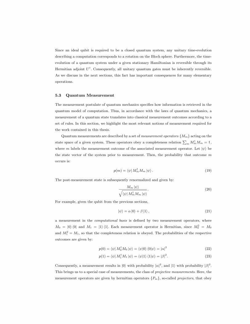
Quantum measurements are described by a set of measurement operators Mm acting on the
state space of a given system. These operators obey a completeness relation∑mM
†mMm = 1,
where m labels the measurement outcome of the associated measurement operator. Let |ψ〉 be
the state vector of the system prior to measurement. Then, the probability that outcome m
occurs is:
p(m) = 〈ψ|M†mMm |ψ〉 . (19)
The post-measurement state is subsequently renormalized and given by:
Mm |ψ〉√〈ψ|M†mMm |ψ〉
. (20)
For example, given the qubit from the previous sections,
|ψ〉 = α |0〉+ β |1〉 , (21)
a measurement in the computational basis is defined by two measurement operators, where
M0 = |0〉 〈0| and M1 = |1〉 〈1|. Each measurement operator is Hermitian, since M20 = M0
and M21 = M1, so that the completeness relation is obeyed. The probabilities of the respective
outcomes are given by:
p(0) = 〈ψ|M†0M0 |ψ〉 = 〈ψ|0〉 〈0|ψ〉 = |α|2 (22)
p(1) = 〈ψ|M†1M1 |ψ〉 = 〈ψ|1〉 〈1|ψ〉 = |β|2. (23)
Consequently, a measurement results in |0〉 with probability |α|2, and |1〉 with probability |β|2.
This brings us to a special case of measurements, the class of projective measurements. Here, the
measurement operators are given by hermitian operators Pm, so-called projectors, that obey
a completeness relation∑m Pm = 1 and satisfy PnPm = δn,mPm.
The probability to observe the outcome m is given by:
p(m) = 〈ψ|Pm |ψ〉 , (24)
whereas the post-measurement state is
Pm |ψ〉√〈ψ|Pm |ψ〉
. (25)
A final class of more general measurements we consider is that of POVM measurements (Positive-
Operator-Valued Measure) [NC10], where the post-measurement state is of little interest and
the concern lies on the outcome probabilities corresponding to a set of measurement operators.
In this context, a set of positive semidefinite measurement operators Em is employed such
that∑mEm = 1.
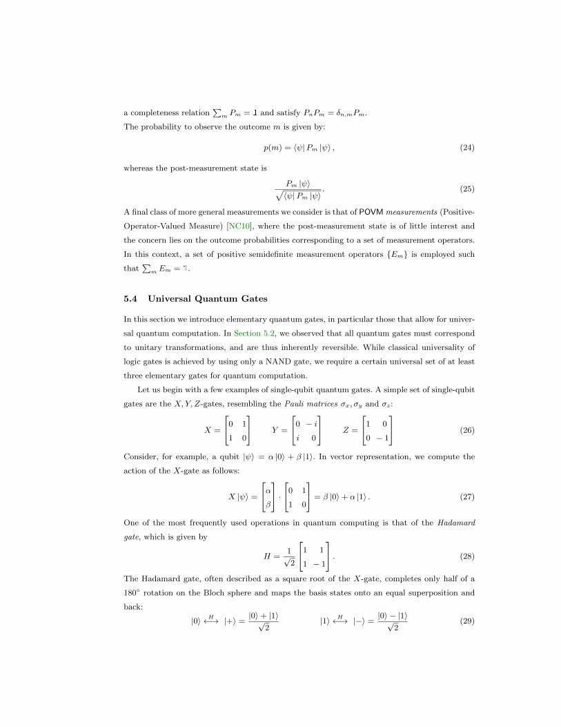
5.4 Universal Quantum Gates
In this section we introduce elementary quantum gates, in particular those that allow for univer-
sal quantum computation. In Section 5.2, we observed that all quantum gates must correspond
to unitary transformations, and are thus inherently reversible. While classical universality of
logic gates is achieved by using only a NAND gate, we require a certain universal set of at least
three elementary gates for quantum computation.
Let us begin with a few examples of single-qubit quantum gates. A simple set of single-qubit
gates are the X,Y, Z-gates, resembling the Pauli matrices σx, σy and σz:
X =
0 1
1 0
Y =
0 − i
i 0
Z =
1 0
0 − 1
(26)
Consider, for example, a qubit |ψ〉 = α |0〉 + β |1〉. In vector representation, we compute the
action of the X-gate as follows:
X |ψ〉 =
αβ
·0 1
1 0
= β |0〉+ α |1〉 . (27)
One of the most frequently used operations in quantum computing is that of the Hadamard
gate, which is given by
H =1√2
1 1
1 − 1
. (28)
The Hadamard gate, often described as a square root of the X-gate, completes only half of a
180 rotation on the Bloch sphere and maps the basis states onto an equal superposition and
back:
|0〉 H←→ |+〉 =|0〉+ |1〉√
2|1〉 H←→ |−〉 =
|0〉 − |1〉√2
(29)
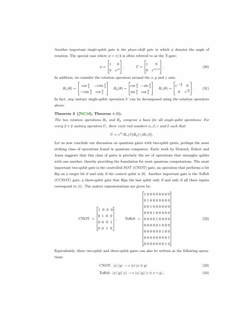
Another important single-qubit gate is the phase-shift gate in which φ denotes the angle of
rotation. The special case where φ = π/4 is often referred to as the T-gate:
φ =
1 0
0 eiφ
, T =
1 0
0 eiπ/4
. (30)
In addition, we consider the rotation operators around the x, y and z axis:
Rx(θ) =
cos θ2−i sin θ
2
−i sin θ2
cos θ2
Ry(θ) =
cos θ2− sin θ
2
sin θ2
cos θ2
Rz(θ) =
e−i θ2 0
0 eiθ2
. (31)
In fact, any unitary single-qubit operation U can be decomposed using the rotation operators
above.
Theorem 3 ([NC10], Theorem 4.10).
The two rotation operations Rx and Ry comprise a basis for all single-qubit operations: For
every 2× 2 unitary operation U , there exist real numbers α, β, γ and δ such that:
U = eiαRx(β)Ry(γ)Rx(δ).
Let us now conclude our discussion on quantum gates with two-qubit gates, perhaps the most
striking class of operations found in quantum computers. Early work by Deutsch, Eckert and
Josza suggests that this class of gates is precisely the set of operations that entangles qubits
with one another, thereby providing the foundation for most quantum computations. The most
important two-qubit gate is the controlled-NOT (CNOT) gate, an operation that performs a bit
flip on a target bit if and only if the control qubit is |0〉. Another important gate is the Toffoli
(CCNOT) gate, a three-qubit gate that flips the last qubit only if and only if all three inputs
correspond to |1〉. The matrix representations are given by:
CNOT =
1 0 0 0
0 1 0 0
0 0 0 1
0 0 1 0
, Toffoli =
1 0 0 0 0 0 0 0 0
0 1 0 0 0 0 0 0 0
0 0 1 0 0 0 0 0 0
0 0 0 1 0 0 0 0 0
0 0 0 0 1 0 0 0 0
0 0 0 0 0 1 0 0 0
0 0 0 0 0 0 1 0 0
0 0 0 0 0 0 0 0 1
0 0 0 0 0 0 0 1 0
(32)
Equivalently, these two-qubit and three-qubit gates can also be written as the following opera-
tions:
CNOT: |x〉 |y〉 −→ |x〉 |x⊕ y〉 (33)
Toffoli: |x〉 |y〉 |z〉 −→ |x〉 |y〉 |z ⊕ x ∧ y〉 , (34)
where ⊕ denotes addition modulo 2 and ∧ denotes the AND operation (Table 1). Finally, we
also consider the controlled-Z (CZ) gate, an operation that features an additional minus sign
and has the following matrix representation:
CZ =
1 0 0 0
0 1 0 0
0 0 1 0
0 0 0 −1
(35)
The following theorem states ensures that quantum computation is indeed universal using only
a limited set of gates.
Theorem 4 ([Deu89] [Kit97], Universal set of quantum operations).
The Hadamard gate, the Toffoli gate and phase-shift gate comprise a universal basis for any
quantum operation: For every D ≥ 3, there exists l ≤ 100(D log 1ε)3 such that every unitary
D ×D matrix U can be approximated by a sequence of the above unitary gates to ε > 0 degree
of accuracy:
|Ui,j − (Ul · · · U1)i,j | < ε,
where the index (i, j) denotes the entries of the respective matrices.
While a basis for quantum computation is not limited to precisely the set as given in Theorem 4,
it nevertheless provides a convenient choice of elementary gates.
5.5 The No-Cloning Theorem
One of the most defining aspects of quantum information is the fact that it cannot be copied.
The no-cloning theorem is attributed to Wooters and Zurek [WZ82] and can in brief be stated
as follows:
There exists no universal quantum operation that can make an identical copy of an unknown
quantum state.
We give a short proof by contradiction, as for example found in [Wil13], that illustrates the
impossibility of such an operation: Suppose there exists a two-qubit operator U with the above
properties. Thus, if we take an arbitrary qubit |ψ〉 = α |0〉+ β |1〉 as input, we expect:
U |ψ〉 |0〉 → |ψ〉 |ψ〉 (36)
= (α |0〉+ β |1〉)(α |0〉+ β |1〉) (37)
= α2 |0〉 |0〉+ αβ |0〉 |1〉+ βα |1〉 |0〉+ β2 |1〉 |1〉 . (38)
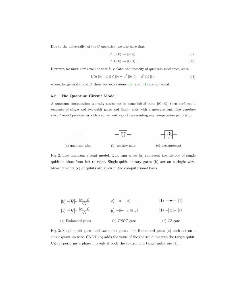
Due to the universality of the U operation, we also have that:
U |0〉 |0〉 → |0〉 |0〉 (39)
U |1〉 |0〉 → |1〉 |1〉 . (40)
However, we must now conclude that U violates the linearity of quantum mechanics, since
U(α |0〉+ β |1〉) |0〉 = α2 |0〉 |0〉+ β2 |1〉 |1〉 , (41)
where, for general α and β, these two expressions (38) and (41) are not equal.
5.6 The Quantum Circuit Model
A quantum computation typically starts out in some initial state |00...0〉, then performs a
sequence of single and two-qubit gates and finally ends with a measurement. The quantum
circuit model provides us with a convenient way of representing any computation pictorially.
(a) quantum wire
U
(b) unitary gate (c) measurement
Fig. 2: The quantum circuit model. Quantum wires (a) represent the history of single
qubit in time from left to right. Single-qubit unitary gates (b) act on a single wire.
Measurements (c) of qubits are given in the computational basis.
|0〉
|1〉
H
H
|0〉+|1〉√2
|0〉−|1〉√2
(a) Hadamard gates
|x〉
|y〉
|x〉
|x⊕ y〉
(b) CNOT-gate
|1〉
|1〉 Z
|1〉
|i〉
(c) CZ-gate
Fig. 3: Single-qubit gates and two-qubit gates. The Hadamard gates (a) each act on a
single quantum wire. CNOT (b) adds the value of the control qubit into the target qubit.
CZ (c) performs a phase flip only if both the control and target qubit are |1〉.
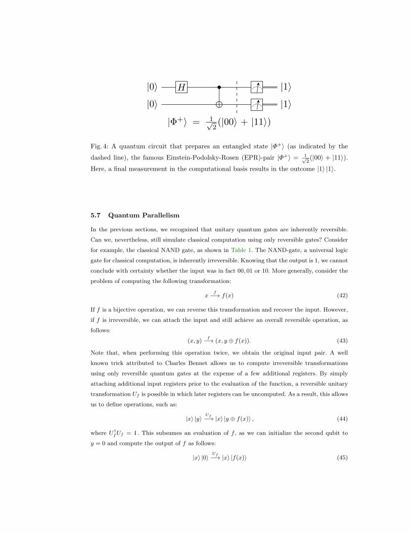
|0〉|0〉
H
|Φ+〉 = 1√2(|00〉 + |11〉)
|1〉|1〉
Fig. 4: A quantum circuit that prepares an entangled state |Φ+〉 (as indicated by the
dashed line), the famous Einstein-Podolsky-Rosen (EPR)-pair |Φ+〉 = 1√2(|00〉 + |11〉).
Here, a final measurement in the computational basis results in the outcome |1〉 |1〉.
5.7 Quantum Parallelism
In the previous sections, we recognized that unitary quantum gates are inherently reversible.
Can we, nevertheless, still simulate classical computation using only reversible gates? Consider
for example, the classical NAND gate, as shown in Table 1. The NAND-gate, a universal logic
gate for classical computation, is inherently irreversible. Knowing that the output is 1, we cannot
conclude with certainty whether the input was in fact 00, 01 or 10. More generally, consider the
problem of computing the following transformation:
xf−→ f(x) (42)
If f is a bijective operation, we can reverse this transformation and recover the input. However,
if f is irreversible, we can attach the input and still achieve an overall reversible operation, as
follows:
(x, y)f−→ (x, y ⊕ f(x)). (43)
Note that, when performing this operation twice, we obtain the original input pair. A well
known trick attributed to Charles Bennet allows us to compute irreversible transformations
using only reversible quantum gates at the expense of a few additional registers. By simply
attaching additional input registers prior to the evaluation of the function, a reversible unitary
transformation Uf is possible in which later registers can be uncomputed. As a result, this allows
us to define operations, such as:
|x〉 |y〉Uf−→ |x〉 |y ⊕ f(x)〉 , (44)
where U†fUf = 1. This subsumes an evaluation of f , as we can initialize the second qubit to
y = 0 and compute the output of f as follows:
|x〉 |0〉Uf−→ |x〉 |f(x)〉 (45)
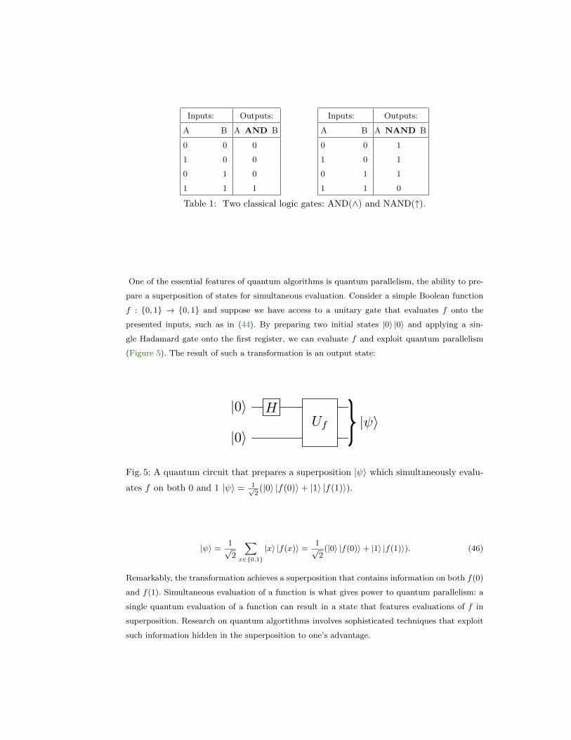
Inputs: Outputs:
A B A AND B
0 0 0
1 0 0
0 1 0
1 1 1
Inputs: Outputs:
A B A NAND B
0 0 1
1 0 1
0 1 1
1 1 0
Table 1: Two classical logic gates: AND(∧) and NAND(↑).
One of the essential features of quantum algorithms is quantum parallelism, the ability to pre-
pare a superposition of states for simultaneous evaluation. Consider a simple Boolean function
f : 0, 1 → 0, 1 and suppose we have access to a unitary gate that evaluates f onto the
presented inputs, such as in (44). By preparing two initial states |0〉 |0〉 and applying a sin-
gle Hadamard gate onto the first register, we can evaluate f and exploit quantum parallelism
(Figure 5). The result of such a transformation is an output state:
|0〉
|0〉
HUf |ψ〉
Fig. 5: A quantum circuit that prepares a superposition |ψ〉 which simultaneously evalu-
ates f on both 0 and 1 |ψ〉 = 1√2(|0〉 |f(0)〉+ |1〉 |f(1)〉).
|ψ〉 =1√2
∑x∈0,1
|x〉 |f(x)〉 =1√2
(|0〉 |f(0)〉+ |1〉 |f(1)〉). (46)
Remarkably, the transformation achieves a superposition that contains information on both f(0)
and f(1). Simultaneous evaluation of a function is what gives power to quantum parallelism: a
single quantum evaluation of a function can result in a state that features evaluations of f in
superposition. Research on quantum algortithms involves sophisticated techniques that exploit
such information hidden in the superposition to one’s advantage.
5.8 Decoherence
As with any physical implementation of a computing device, not all operations can be done
perfectly and there remains an unavoidable risk of error. Typically, one distinguishes between
two classes of errors. We encounter both memory errors that occur during storage of information,
as well as operational errors that occur during manipulation of stored information. In the section
on error correcting codes, we provide further discussion on how to correct for such errors.
Quantum Noise Models. In order to develop a successful noise model, we follow [NC10] and
adopt a theory of quantum channels and the operator-sum-representation. In this framework,
we consider noise models as discrete state changes without reference to time.
For the remainder of the section, we let % be a quantum system of computational states |0〉
and |1〉 and define the action of a noisy quantum channel by a completely positive and trace
preserving (CPTP) operation E , where for operation elements E0 and E1, we have:
% −→ E(%) = E0%E†0 + E1%E
†1 . (47)
A simple quantum noise channel is the bit-flip channel that, with probability η > 0, maps the
state |0〉 to the state |1〉 and vice-versa:
E0 =√
1− η ·
1 0
0 1
, E1 =√η ·
0 1
1 0
. (48)
Thus, in the operator-sum-representation, we can now write the bit-flip channel as:
% −→ EX(%) = (1− η)%+ η X%X†, (49)
where X corresponds to the bit-flip gate from the earlier sections.
Consider now the case of a single qubit, a quantum system that starts out in a pure state
% = |ψ〉 〈ψ|, where |ψ〉 = α |0〉 + β |1〉. Under the bit-flip channel E , the state evolves into a
statistical mixture according to (49). Therefore, with probability 1− η, we recover the original
state,
|ψ〉 = α |0〉+ β |1〉 , (50)
and, with probability η, we find the system in a state:
|ψ⊥〉 = β |0〉+ α |1〉 . (51)
This noise model is often called classification noise and will be highly relevant for the quantum
learning algorithms of the later sections.
Another elementary quantum noise channel is the phase-flip channel that, with probability
η > 0, maps the state |1〉 to the state − |1〉, where
E0 =√
1− η ·
1 0
0 1
, E1 =√η ·
1 0
0 − 1
. (52)
Thus, in the operator-sum-representation, we can also write the phase-flip channel as:
% −→ EZ(%) = (1− η)%+ η Z%Z†, (53)
where Z corresponds to the phase-flip gate from the earlier sections.
A much more ideal noise model for quantum computation is the amplitude damping channel.
This noise channel EAD corresponds to a scenario in which a photon is spontaneously emitted
with some probability γ.
% −→ EAD(%) = E0%E†0 + E1%E
†1 , (54)
where the transition matrix operators are given by:
E0 =
1 0
0√
1− γ
, E1 =
1√γ
0 0
. (55)
Thus, E1 corresponds to the emission of a photon and a quantum of energy is lost to the
environment. The operator E0, corresponds to the case where the state remains unchanged and
a photon is not yet lost but the amplitudes are adjusted appropriately.
Finally, we consider the depolarizing channel, a devastating type of noise model in which
all quantum information is lost to the environment and the quantum state gets replaced by a
maximally mixed state with some probability η:
% −→ ED(%) = (1− η)%+ η1
2, (56)
where 1
2is the maximally mixed state.
Independent Noise Models. The most commonly adopted noise model in computational
learning theory is that of independent noise. For example, in the LWE probblem each state or
sample is independently corrupted by some probability. Most generally in the context of qubits,
we consider independent noise by extending the noise models from this section onto quantum
registers. Consider a register of n qubits |Ψ〉, where
|Ψ〉 =∑
x∈0,1nαx |x1〉 |x2〉 ... |xn〉 . (57)
By, for example, extending the bit-flip channel from this section independently onto the entire
register, the result is a state
|Ψ〉 =∑
x∈0,1nαx |x1 ⊕ e1〉 |x2 ⊕ e2〉 ... |xn ⊕ en〉 , (58)
where each error ei is sampled from a Bernoulli distribution of noise rate η > 0:
Bern(η) =
1, with probability η
0, with probability 1− η.(59)
Note that, upon a choice of error distribution, an independent noise model also translates nat-
urally in the context of qudits instead of qubits.
5.9 Error Correcting Codes
In his seminal 1948 paper A Mathematical Theory of Communication [Sha48], Claude Shannon
put forward a revolutionary view on the concept information and errors in communication. In-
stead of investing tedious effort to avoid them on a technical level, it is not only possible, but
oftentimes even favorable, to simply correct them. In the 1950s, John von Neumann developed
very successful error correcting codes in order to address noise originating in the relay archi-
tecture of present computer technology. Today’s transistors achieve near-perfect fault tolerance,
hence error correcting codes often do not even have to be applied. In a nutshell, by adding
additional redundant information to each bit of information, one can realize error correction.
Suppose the task is to store a single bit of information for some desired time interval T ≥ 0.
Regardless of whether an operation takes place, we consider memory errors that can occur
spontaneously. We denote the probability that such an error occurs after time T by p. A simple
way to protect the storage of information against these affects is by adding redundance. For
example, consider the following three copies of each instance of the bit:
0 −→ 000 (60)
1 −→ 111. (61)
The probability that there are no errors is given by (1 − p)3. Hence, after time T , the three
bits 000 remain the same. The probability that there is an error in one of the bits is 3p(1− p)2,
resulting in either 001, 010 or 100. Finally, the probability that there are two or more errors is
3p2(1 − p) + p3. The error correction scheme now works as follows. By measuring all the bits
and taking the majority vote, we can easily rule out single bit errors. Our correction method
thus assigns the measurement outcomes of the bitstrings as follows:
000, 001, 010, 100 −→ 0 (62)
111, 110, 101, 011 −→ 1. (63)
The error correction method above is correct with probability pc = 1 − 3p2 + 2p3. Compared
to the previous error probability of p, we gain as long as pc ≥ 1 − p. This translates into an
error probability of at most p < 12. By dividing the time interval into slices ∆t = T/N and
applying the error correcting code repeatedly after reach slice, one can reach arbitrarily close
success probabilities which grow in N [NC10][CZ01].
Consider now the problem of quantum error correction by analogy to classical error correc-
tion. Due to the quantum nature of information, a new framework is needed to correct for errors.
This becomes apparent as we consider a number of differences as compared to classical error cor-
rection. According to the no-cloning theorem 5.5, there is no machine that can make a copy of an
unknown quantum state. Therefore, the naive attempt of simply copying quantum information
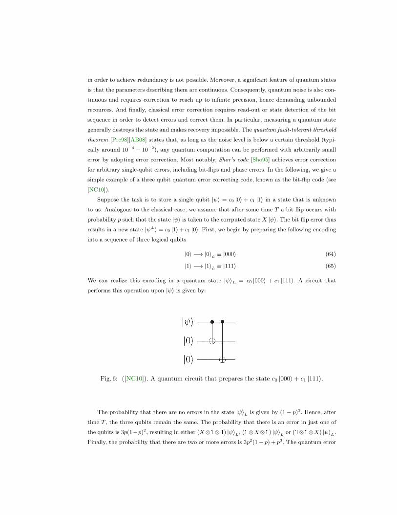
in order to achieve redundancy is not possible. Moreover, a signifcant feature of quantum states
is that the parameters describing them are continuous. Consequently, quantum noise is also con-
tinuous and requires correction to reach up to infinite precision, hence demanding unbounded
recources. And finally, classical error correction requires read-out or state detection of the bit
sequence in order to detect errors and correct them. In particular, measuring a quantum state
generally destroys the state and makes recovery impossible. The quantum fault-tolerant threshold
theorem [Pre98][AB08] states that, as long as the noise level is below a certain threshold (typi-
cally around 10−4 − 10−2), any quantum computation can be performed with arbitrarily small
error by adopting error correction. Most notably, Shor’s code [Sho95] achieves error correction
for arbitrary single-qubit errors, including bit-flips and phase errors. In the following, we give a
simple example of a three qubit quantum error correcting code, known as the bit-flip code (see
[NC10]).
Suppose the task is to store a single qubit |ψ〉 = c0 |0〉 + c1 |1〉 in a state that is unknown
to us. Analogous to the classical case, we assume that after some time T a bit flip occurs with
probability p such that the state |ψ〉 is taken to the corrputed state X |ψ〉. The bit flip error thus
results in a new state |ψ⊥〉 = c0 |1〉+ c1 |0〉. First, we begin by preparing the following encoding
into a sequence of three logical qubits
|0〉 −→ |0〉L ≡ |000〉 (64)
|1〉 −→ |1〉L ≡ |111〉 . (65)
We can realize this encoding in a quantum state |ψ〉L = c0 |000〉 + c1 |111〉. A circuit that
performs this operation upon |ψ〉 is given by:
Fig. 6: ([NC10]). A quantum circuit that prepares the state c0 |000〉+ c1 |111〉.
The probability that there are no errors in the state |ψ〉L is given by (1− p)3. Hence, after
time T , the three qubits remain the same. The probability that there is an error in just one of
the qubits is 3p(1−p)2, resulting in either (X⊗1⊗1) |ψ〉L, (1⊗X⊗1) |ψ〉L or (1⊗1⊗X) |ψ〉L.
Finally, the probability that there are two or more errors is 3p2(1− p) + p3. The quantum error
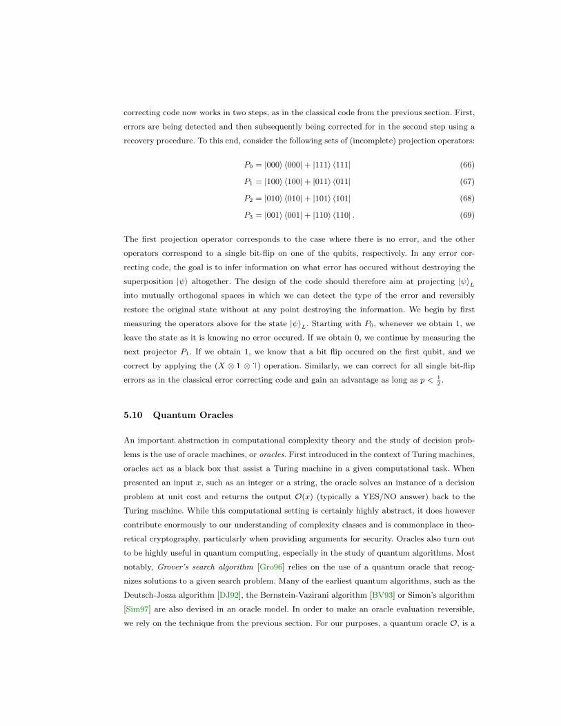
correcting code now works in two steps, as in the classical code from the previous section. First,
errors are being detected and then subsequently being corrected for in the second step using a
recovery procedure. To this end, consider the following sets of (incomplete) projection operators:
P0 = |000〉 〈000|+ |111〉 〈111| (66)
P1 = |100〉 〈100|+ |011〉 〈011| (67)
P2 = |010〉 〈010|+ |101〉 〈101| (68)
P3 = |001〉 〈001|+ |110〉 〈110| . (69)
The first projection operator corresponds to the case where there is no error, and the other
operators correspond to a single bit-flip on one of the qubits, respectively. In any error cor-
recting code, the goal is to infer information on what error has occured without destroying the
superposition |ψ〉 altogether. The design of the code should therefore aim at projecting |ψ〉Linto mutually orthogonal spaces in which we can detect the type of the error and reversibly
restore the original state without at any point destroying the information. We begin by first
measuring the operators above for the state |ψ〉L. Starting with P0, whenever we obtain 1, we
leave the state as it is knowing no error occured. If we obtain 0, we continue by measuring the
next projector P1. If we obtain 1, we know that a bit flip occured on the first qubit, and we
correct by applying the (X ⊗ 1 ⊗ 1) operation. Similarly, we can correct for all single bit-flip
errors as in the classical error correcting code and gain an advantage as long as p < 12.
5.10 Quantum Oracles
An important abstraction in computational complexity theory and the study of decision prob-
lems is the use of oracle machines, or oracles. First introduced in the context of Turing machines,
oracles act as a black box that assist a Turing machine in a given computational task. When
presented an input x, such as an integer or a string, the oracle solves an instance of a decision
problem at unit cost and returns the output O(x) (typically a YES/NO answer) back to the
Turing machine. While this computational setting is certainly highly abstract, it does however
contribute enormously to our understanding of complexity classes and is commonplace in theo-
retical cryptography, particularly when providing arguments for security. Oracles also turn out
to be highly useful in quantum computing, especially in the study of quantum algorithms. Most
notably, Grover’s search algorithm [Gro96] relies on the use of a quantum oracle that recog-
nizes solutions to a given search problem. Many of the earliest quantum algorithms, such as the
Deutsch-Josza algorithm [DJ92], the Bernstein-Vazirani algorithm [BV93] or Simon’s algorithm
[Sim97] are also devised in an oracle model. In order to make an oracle evaluation reversible,
we rely on the technique from the previous section. For our purposes, a quantum oracle O, is a
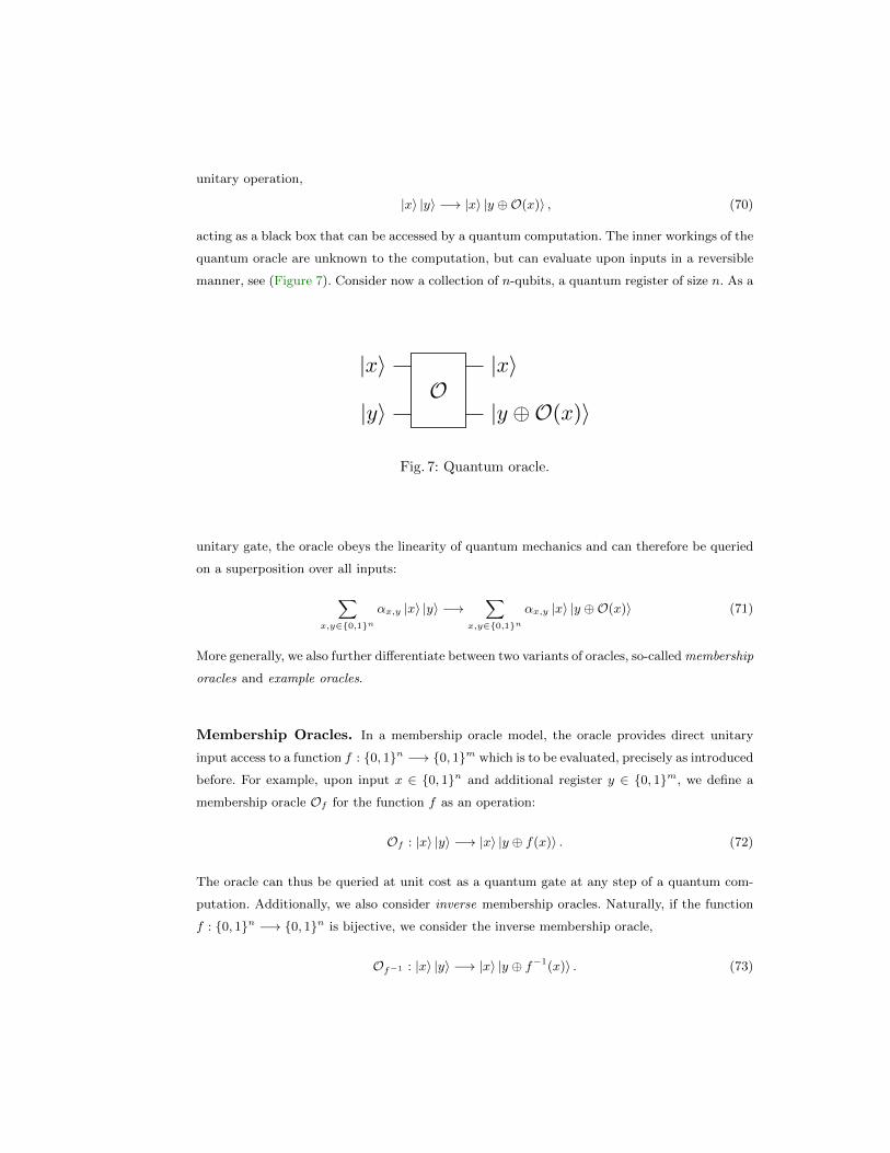
unitary operation,
|x〉 |y〉 −→ |x〉 |y ⊕O(x)〉 , (70)
acting as a black box that can be accessed by a quantum computation. The inner workings of the
quantum oracle are unknown to the computation, but can evaluate upon inputs in a reversible
manner, see (Figure 7). Consider now a collection of n-qubits, a quantum register of size n. As a
|x〉
|y〉O
|x〉
|y ⊕O(x)〉
Fig. 7: Quantum oracle.
unitary gate, the oracle obeys the linearity of quantum mechanics and can therefore be queried
on a superposition over all inputs:
∑x,y∈0,1n
αx,y |x〉 |y〉 −→∑
x,y∈0,1nαx,y |x〉 |y ⊕O(x)〉 (71)
More generally, we also further differentiate between two variants of oracles, so-called membership
oracles and example oracles.
Membership Oracles. In a membership oracle model, the oracle provides direct unitary
input access to a function f : 0, 1n −→ 0, 1m which is to be evaluated, precisely as introduced
before. For example, upon input x ∈ 0, 1n and additional register y ∈ 0, 1m, we define a
membership oracle Of for the function f as an operation:
Of : |x〉 |y〉 −→ |x〉 |y ⊕ f(x)〉 . (72)
The oracle can thus be queried at unit cost as a quantum gate at any step of a quantum com-
putation. Additionally, we also consider inverse membership oracles. Naturally, if the function
f : 0, 1n −→ 0, 1n is bijective, we consider the inverse membership oracle,
Of−1 : |x〉 |y〉 −→ |x〉 |y ⊕ f−1(x)〉 . (73)
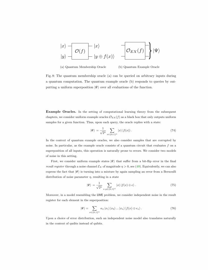
|x〉
|y〉O(f)
|x〉
|y ⊕ f(x)〉
(a) Quantum Membership Oracle
OEX(f) |Ψ〉
(b) Quantum Example Oracle
Fig. 8: The quantum membership oracle (a) can be queried on arbitrary inputs during
a quantum computation. The quantum example oracle (b) responds to queries by out-
putting a uniform superposition |Ψ〉 over all evaluations of the function.
Example Oracles. In the setting of computational learning theory from the subsequent
chapters, we consider uniform example oracles OEX(f) as a black box that only outputs uniform
samples for a given function. Thus, upon each query, the oracle replies with a state:
|Ψ〉 =1√2n
∑x∈0,1n
|x〉 |f(x)〉 . (74)
In the context of quantum example oracles, we also consider samples that are corrupted by
noise. In particular, as the example oracle consists of a quantum circuit that evaluates f on a
superposition of all inputs, this operation is naturally prone to errors. We consider two models
of noise in this setting.
First, we consider uniform example states |Ψ〉 that suffer from a bit-flip error in the final
result register through a noise channel EX of magnitude η > 0, see (49). Equivalently, we can also
express the fact that |Ψ〉 is turning into a mixture by again sampling an error from a Bernoulli
distribution of noise parameter η, resulting in a state
|Ψ〉 =1√2n
∑x,y∈0,1n
|x〉 |f(x)⊕ e〉 . (75)
Moreover, in a model resembling the LWE problem, we consider independent noise in the result
register for each element in the superposition:
|Ψ〉 =∑
x∈0,1nαx |x1〉 |x2〉 ... |xn〉 |f(x)⊕ ex〉 . (76)
Upon a choice of error distribution, such an independent noise model also translates naturally
in the context of qudits instead of qubits.
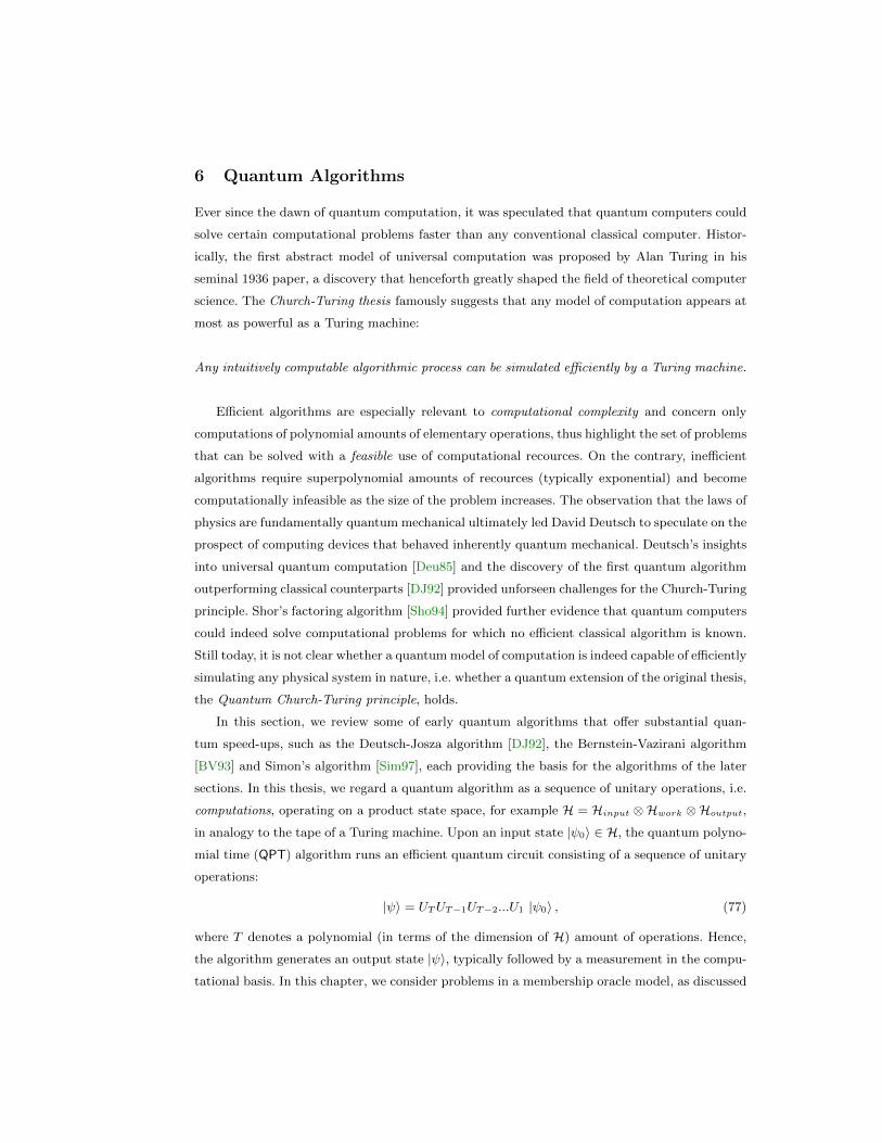
6 Quantum Algorithms
Ever since the dawn of quantum computation, it was speculated that quantum computers could
solve certain computational problems faster than any conventional classical computer. Histor-
ically, the first abstract model of universal computation was proposed by Alan Turing in his
seminal 1936 paper, a discovery that henceforth greatly shaped the field of theoretical computer
science. The Church-Turing thesis famously suggests that any model of computation appears at
most as powerful as a Turing machine:
Any intuitively computable algorithmic process can be simulated efficiently by a Turing machine.
Efficient algorithms are especially relevant to computational complexity and concern only
computations of polynomial amounts of elementary operations, thus highlight the set of problems
that can be solved with a feasible use of computational recources. On the contrary, inefficient
algorithms require superpolynomial amounts of recources (typically exponential) and become
computationally infeasible as the size of the problem increases. The observation that the laws of
physics are fundamentally quantum mechanical ultimately led David Deutsch to speculate on the
prospect of computing devices that behaved inherently quantum mechanical. Deutsch’s insights
into universal quantum computation [Deu85] and the discovery of the first quantum algorithm
outperforming classical counterparts [DJ92] provided unforseen challenges for the Church-Turing
principle. Shor’s factoring algorithm [Sho94] provided further evidence that quantum computers
could indeed solve computational problems for which no efficient classical algorithm is known.
Still today, it is not clear whether a quantum model of computation is indeed capable of efficiently
simulating any physical system in nature, i.e. whether a quantum extension of the original thesis,
the Quantum Church-Turing principle, holds.
In this section, we review some of early quantum algorithms that offer substantial quan-
tum speed-ups, such as the Deutsch-Josza algorithm [DJ92], the Bernstein-Vazirani algorithm
[BV93] and Simon’s algorithm [Sim97], each providing the basis for the algorithms of the later
sections. In this thesis, we regard a quantum algorithm as a sequence of unitary operations, i.e.
computations, operating on a product state space, for example H = Hinput ⊗Hwork ⊗Houtput,
in analogy to the tape of a Turing machine. Upon an input state |ψ0〉 ∈ H, the quantum polyno-
mial time (QPT) algorithm runs an efficient quantum circuit consisting of a sequence of unitary
operations:
|ψ〉 = UTUT−1UT−2...U1 |ψ0〉 , (77)
where T denotes a polynomial (in terms of the dimension of H) amount of operations. Hence,
the algorithm generates an output state |ψ〉, typically followed by a measurement in the compu-
tational basis. In this chapter, we consider problems in a membership oracle model, as discussed
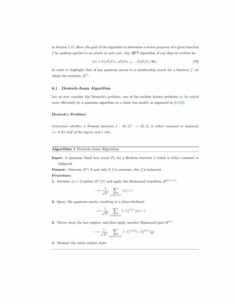
in Section 5.10. Here, the goal of the algorithm is determine a secret property of a given function
f by making queries to an oracle at unit cost. Any QPT algorithm A can thus be written as:
|ψ〉 = UTOfUT−1OfUT−2 . . . U2OfU1 |Ψ0〉 . (78)
In order to highlight that A has quantum access to a membership oracle for a function f , we
adopt the notation A|f〉.
6.1 Deutsch-Josza Algorithm
Let us now consider the Deutsch’s problem, one of the earliest known problems to be solved
more efficiently by a quantum algorithm in a black box model, as appeared in [DJ92]:
Deutsch’s Problem:
Determine whether a Boolean function f : 0, 1n → 0, 1 is either constant or balanced,
i.e. 0 for half of the inputs and 1 else.
Algorithm 1 Deutsch-Josza Algorithm
Input: A quantum black box oracle Of for a Boolean function f which is either constant or
balanced.
Output: Outcome |0n〉 if and only if f is constant, else f is balanced.
Procedure:
1. Initialize (n+ 1)-qubits |0n〉 |1〉 and apply the Hadamard transform H⊕(n+1):
−→ 1√2n
∑x∈0,1n
|x〉 |−〉
2. Query the quantum oracle, resulting in a phase-kickback :
−→ 1√2n
∑x∈0,1n
(−1)f(x) |x〉 |−〉
3. Throw away the last register and then apply another Hadamard gate H⊗n:
−→ 1√2n
∑x,y∈0,1n
(−1)〈x,y〉(−1)f(x) |y〉
4. Measure the entire output state.
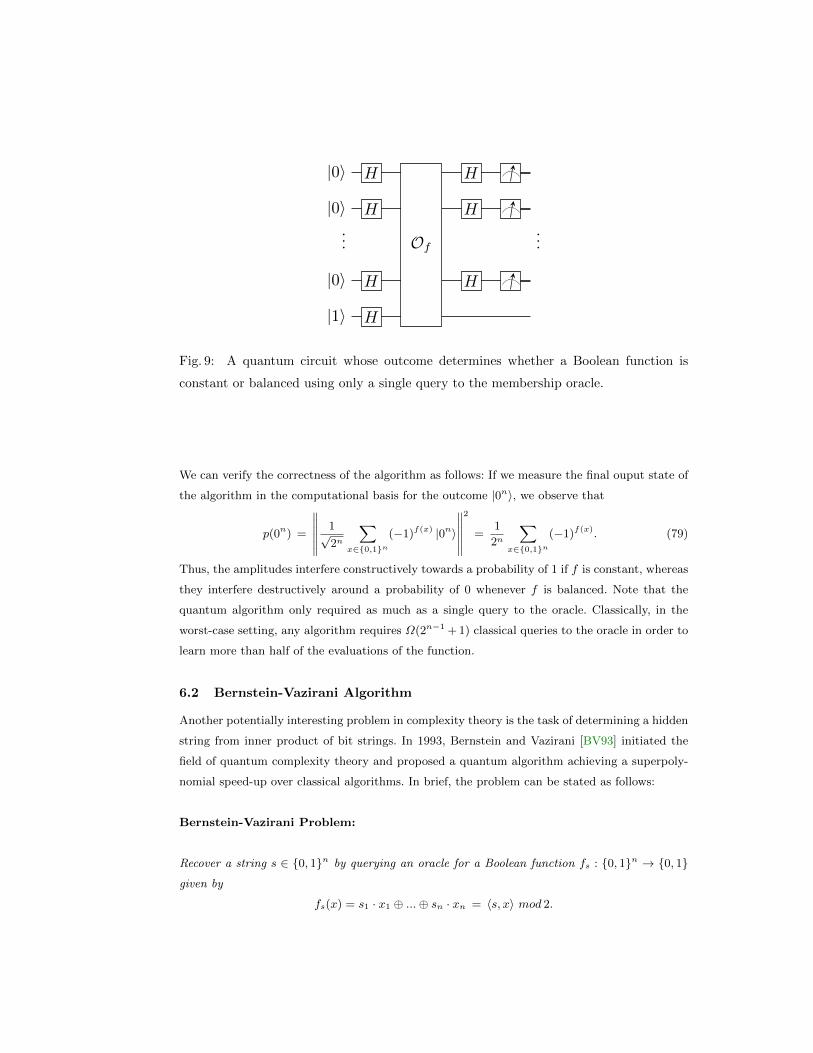
|0〉
|0〉...
|0〉
|1〉
H
H
H
H
Of
H
H
H
...
Fig. 9: A quantum circuit whose outcome determines whether a Boolean function is
constant or balanced using only a single query to the membership oracle.
We can verify the correctness of the algorithm as follows: If we measure the final ouput state of
the algorithm in the computational basis for the outcome |0n〉, we observe that
p(0n) =
∥∥∥∥∥∥ 1√2n
∑x∈0,1n
(−1)f(x) |0n〉
∥∥∥∥∥∥2
=1
2n
∑x∈0,1n
(−1)f(x). (79)
Thus, the amplitudes interfere constructively towards a probability of 1 if f is constant, whereas
they interfere destructively around a probability of 0 whenever f is balanced. Note that the
quantum algorithm only required as much as a single query to the oracle. Classically, in the
worst-case setting, any algorithm requires Ω(2n−1 + 1) classical queries to the oracle in order to
learn more than half of the evaluations of the function.
6.2 Bernstein-Vazirani Algorithm
Another potentially interesting problem in complexity theory is the task of determining a hidden
string from inner product of bit strings. In 1993, Bernstein and Vazirani [BV93] initiated the
field of quantum complexity theory and proposed a quantum algorithm achieving a superpoly-
nomial speed-up over classical algorithms. In brief, the problem can be stated as follows:
Bernstein-Vazirani Problem:
Recover a string s ∈ 0, 1n by querying an oracle for a Boolean function fs : 0, 1n → 0, 1
given by
fs(x) = s1 · x1 ⊕ ...⊕ sn · xn = 〈s, x〉 mod 2.
In the classical membership oracle setting, we observe that a single query to the function can
only ever reveal as much as one bit of information about the secret string s. In fact, this can
easily be done by considering queries on strings ei = (0, ... , 1, ... , 0), where the i-th index is 1
and ei is 0 everywhere else. An algorithm performing such queries achieves an overall query
complexity of Ω(n) when determining the secret, as each iteration reveals only a single bit of
the hidden string by querying
fs(ei) = 〈s, ei〉 mod 2 = si, (80)
so that s is fully determined after a total of n queries to the function.
In the quantum membership oracle model, Bernstein and Vazirani showed that only a single
quantum query to the oracle is sufficient [BV93]:
Algorithm 2 Bernstein-Vazirani Algorithm
Input: A quantum black box oracle Ofs for a Boolean function fs, where fs(x) = 〈s, x〉. The
task is to determine s ∈ 0, 1n.
Output: The secret string with only a single query to the oracle.
Procedure:
1. Initialize (n+ 1)-qubits to |0n〉 |1〉 and apply the Hadamard transform H⊕(n+1):
−→ 1√2n
∑x∈0,1n
|x〉 |−〉
2. Query the quantum oracle, resulting in a phase-kickback :
−→ 1√2n
∑x∈0,1n
(−1)〈s,x〉 |x〉 |−〉
3. Throw away the last register and then apply a Hadamard gate H⊗n:
−→ 1√2n
∑x,y∈0,1n
(−1)〈s,x〉(−1)x·y |y〉
4. Measure the entire output state.
|0〉
|0〉...
|0〉
|1〉
H
H
H
H
Ofs
H
H
H
...
Fig. 10: A quantum circuit for the Bernstein-Vazirani problem. The secret string is
determined after only a single query to the membership oracle.
Thus, if we now measure the final ouput state of the algorithm in the computational basis for a
particular outcome m ∈ 0, 1n, we observe that
p(m) =
∥∥∥∥∥∥ 1√2n
∑x∈0,1n
(−1)〈s,x〉(−1)x·m |m〉
∥∥∥∥∥∥2
(81)
=1
2n
∑x∈0,1n
(−1)(s1⊕m1)x1(−1)(s2⊕m2)x2 · · · (−1)(sn⊕mn)xn (82)
=1
2n
∑x1∈0,1
(−1)(s1⊕m1)x1
∑x2∈0,1
(−1)(s2⊕m2)x2
· · · ∑xn∈0,1
(−1)(sn⊕mn)xn
=
1
2n
n∏j=1
1∑xj=0
(−1)(sj⊕mj)xj (83)
=1
2n
n∏j=1
(1 + (−1)sj⊕mj
). (84)
Note that the probabilities of measuring any output states m 6= s vanish due to (84). Conse-
quently, the amplitudes interfere constructively towards a probability of 1 if every bit of the
output state m is equal to s.
7 The Quantum Fourier Transform
The quantum Fourier transform (QFT) is arguably the most important and most widely used
tool in the design of quantum algorithms. Many of the known algorithms, such as the Deutsch-
Josza algorithm, Shor’s factoring algorithm, quantum phase estimation, quantum order finding,
Simon’s algorithm [Sim97] or the Bernstein-Vazirani algorithm rely substantially on its use. In
the previous section, we encountered the Hadamard transform as a single qubit gate H that
performs the following operation:
H |x〉 =1√2
1∑y=0
(−1)x·y |y〉. (85)
Implicitly, we have already encountered the single-qubit quantum Fourier transform of order
n = 1. In fact, the Hadamard transform can be thought of as a QFT over the group Z/2Z
that takes single qubits in the computational basis and maps them to the Hadamard basis. The
underlying principle of the Fourier transform already starts to show, namely, that the QFT acts
as a change of basis in which the amplitudes of individual states of the computational basis are
related to the amplitudes of the entire computational space. The amplitudes of the transformed
states are the so-called characters of the Fourier transform.
In this chapter, our goal is to introduce a general qudit extension of the Hadamard transform,
the QFT on the cyclic group Z/qZ, where q is any integer. By extension, we also obtain the QFT
over any finite Abelian group. More importantly, we discuss how the QFT can be efficiently
implemented on a quantum computer. Historically, the earliest non-trivial variant known to be
efficiently computable on a quantum computer is the Fourier transform over the group Z/2nZ,
due to Deutsch [Deu85]. The general variant of the quantum Fourier transform where q is an
arbitrary integer is less common, but also mentioned as a side note in [NC10]. Kitaev [Kit95]
was the first to generalize this variant of the Fourier transform using quantum phase estimation.
Evidently, this breakthrough immediately led to the generalization over finite Abelian groups,
as we will discuss in detail in the next section. In both cases, we review efficient quantum circuit
implementations and thus provide the basis for addressing the QFT in the extended Bernstein-
Vazirani problem.
7.1 The Quantum Fourier Transform over Finite Abelian Groups
The Fourier transform can be defined on arbitrary groups and we can extend the same principle
of basis change into the language of groups and group algebras. For further reading on the
Fourier transform on groups, we refer to the survey [CD10] or the supplementary chapters in
[NC10]. In this thesis, we concern ourselves with the case of finite Abelian groups.
Consider a finite Abelian group (G, ∗) of order |G| = N and let CG = span|g〉 : g ∈ G be the
associated group algebra of G over C. Each element |x〉 ∈ CG can be uniquely expressed as a
linear combination of basis vectors and complex coefficients:
|x〉 =∑g∈G
αg |g〉 , where αg ∈ C. (86)
Since G is finite Abelian, there exists a basis G ⊆ CG of dimension |G| = N that consists of
N distinct irreducible characters χ ∈ G, where χ : G −→ C and χ(a ∗ b) = χ(a) · χ(b) ([CD10],
Appendix B). Moreover, if χ, χ′ ∈ G are two irreducible characters, then:∑x∈G
χ(x) ∗ χ′(x) = N δχ,χ′ . (87)
Definition 9. Let (G, ∗) be a finite Abelian group of order |G| = N and let G be the basis
containing the set of N distinct characters χ : G −→ C.
The quantum Fourier transform FG on the group G is defined as the operation:
|x〉 −→ 1√N
∑χ∈G
χ(x) |χ〉 . (88)
Consider now the case where G is given by the group G = (Z/NZ,+) and N is any integer. In
this case, the irreducible characters χ : Z/NZ −→ C are given precisely by the primitive N th
roots of unity ωN = e2πiN . Thus, for every y ∈ Z/NZ, the character χy(x) = ωxyN is uniquely
determined. By choosing an orthonormal basis |0〉 , |1〉 , ..., |N〉 of G in Fourier space, we can
identify (88) as:
|x〉 −→ 1√N
∑y∈Z/NZ
ωx·yN |y〉 . (89)
Furthermore, we can associate the Fourier transform FG with the operator:
FG =1√N
∑x,y∈Z/NZ
ωx·yN |y〉 〈x| . (90)
Let us briefly state the following fact, analogous to as in Eq.(87), regarding orthogonality of the
roots of unity:
Proposition 1. ∑y∈Z/NZ
ωx·yN ω−x′·y
N = N δx,x′ . (91)
Proof. Consider first the case when x = x′. Then, for all y ∈ Z/NZ, we find ω(x−x′)yN = 1 and
the above sum clearly adds up to N . If x 6= x′, we can apply the partial sum formula of the
geometric series and compute:
1 + ωx−x′
N + (ωx−x′
N )2 + ...+ (ωx−x′
N )N−1 =1− (ωx−x
′
N )N
1− ωx−x′N
= 0. (92)
We can apply Proposition 1 in order to show that FG is indeed a well defined unitary operation:
FGF†G =1
N
∑x,y∈Z/NZ
ωx·yN |x〉 〈y|∑
x′,y′∈Z/NZ
ω−y′·x′
N |y′〉 〈x′| (93)
=1
N
∑x,x′,y,y′∈Z/NZ
ωx·y−x′·y′
N δy,y′ |x〉 〈x′| (94)
=1
N
∑x,x′,y∈Z/NZ
ω(x−x′)·yN |x〉 〈x′| =
∑x,x′∈Z/NZ
δx,x′ |x〉 〈x′| = 1. (95)
According to the fundamental classification of finite abelian groups [CD10], any finite Abelian
group G is structurally equivalent, i.e. isomorphic, to a direct product of cyclic factors whose
orders are prime powers. Let |G| = N and let N = pr11 . . . prkk be the unique prime factorization
of N , then:
G ∼= Z/pr11 Z× . . .× Z/prkk Z. (96)
Moreover, the basis G of irreducible characters is given by products of irreducible characters of
the respective factors in (96). Consequently, following [CD10], the quantum Fourier transform
on finite Abelian groups G is given by:
FG = FZ/pr11 Z ⊗ . . .⊗FZ/prkk Z. (97)
For example, let G = ((Z/NZ)n ,+). Then, for any y ∈ (Z/NZ)n, we can associate a unique
irreducible character χy : Z/NZ −→ C such that for all x ∈ (Z/NZ)n:
χy(x) = χy(x1) · · · χy(xn) = ωx1·y1+...+xn·ynN . (98)
Hence, the quantum Fourier transform FG over the group G = (Z/NZ)n is given by:
|x1〉 |x2〉 . . . |xn〉 −→1√Nn
∑y∈(Z/NZ)n
ωx1·y1+...+xn·ynN |y1〉 |y2〉 . . . |yn〉 , (99)
where, from now on, 〈x, y〉 = x1 ·y1 + . . .+xn ·yn. In the following sections, we consider different
variants of groupsG and derive a quantum circuit implementation that realizes the corresponding
Fourier transformations. Before we give efficient circuit implementations, we require additional
remarks.
Let G be the group G = (Z/NZ,+) and consider the shift operator U(1) that performs the the
following operation:
U(1) : |x〉 −→ |x+ 1〉 , (100)
where x + 1 is the cyclic addition mod N . We can verify that U(1) =∑x∈Z/NZ |x+ 1〉 〈x| is
unitary, since:
U(1)U(1)† =∑
x∈Z/NZ
|x+ 1〉 〈x|∑
x′∈Z/NZ
|x′〉 〈x′ + 1| (101)
=∑
x,x′∈Z/NZ
|x+ 1〉 〈x|x′〉 〈x′ + 1| =∑
x∈Z/NZ
|x+ 1〉 〈x+ 1| = 1. (102)
Therfore, we can prove the following statement that connects our previous discussion on the
quantum Fourier transform with the shift operator, as appeared in the work of Kitaev [Kit95]:
Proposition 2. The shift operator U(1) is diagonal in the Fourier basis:
FG U(1)F†G =∑
y∈Z/NZ
ωyN |y〉 〈y| . (103)
Proof. Let the operators be represented by:
FG =1√N
∑x,y∈Z/NZ
ωx·yN |y〉 〈x| , U(1) =∑
z∈Z/NZ
|z + 1〉 〈z| and
F†G =1√N
∑x′,y′∈Z/NZ
ω−y′·x′
N |y′〉 〈x′| .
Using Proposition 1, we compute:
FG U(1)F†G =1
N
∑x,y,x′,y′∈Z/NZ
ωx·yN ω−y′·x′
N |y〉 〈x | y′ + 1〉 〈x′| (104)
=1
N
∑y,x′,y′∈Z/NZ
ω(y′+1)·yN ω−y
′·x′N |y〉 〈x′| (105)
=∑
y,x′∈Z/NZ
ωyN
1
N
∑y′∈Z/NZ
ωy′·yN ω−y
′·x′N
|y〉 〈x′| (106)
=∑
y,x′∈Z/NZ
ωyN δy,x′ |y〉 〈x′| (107)
=∑
y∈Z/NZ
ωyN |y〉 〈y| . (108)
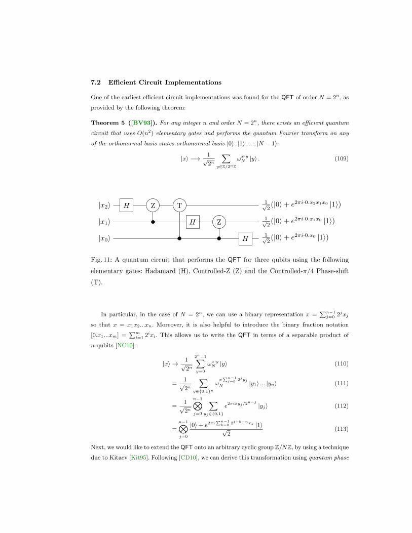
7.2 Efficient Circuit Implementations
One of the earliest efficient circuit implementations was found for the QFT of order N = 2n, as
provided by the following theorem:
Theorem 5 ([BV93]). For any integer n and order N = 2n, there exists an efficient quantum
circuit that uses O(n2) elementary gates and performs the quantum Fourier transform on any
of the orthonormal basis states orthonormal basis |0〉 , |1〉 , ..., |N − 1〉:
|x〉 −→ 1√2n
∑y∈Z/2nZ
ωx·yN |y〉 . (109)
|x2〉
|x1〉
|x0〉
H Z T
H Z
H
1√2(|0〉+ e2πi·0.x2x1x0 |1〉)
1√2(|0〉+ e2πi·0.x1x0 |1〉)
1√2(|0〉+ e2πi·0.x0 |1〉)
Fig. 11: A quantum circuit that performs the QFT for three qubits using the following
elementary gates: Hadamard (H), Controlled-Z (Z) and the Controlled-π/4 Phase-shift
(T).
In particular, in the case of N = 2n, we can use a binary representation x =∑n−1j=0 2jxj
so that x = x1x2...xn. Moreover, it is also helpful to introduce the binary fraction notation
[0.x1...xm] =∑mi=1 2ixi. This allows us to write the QFT in terms of a separable product of
n-qubits [NC10]:
|x〉 → 1√2n
2n−1∑y=0
ωx·yN |y〉 (110)
=1√2n
∑y∈0,1n
ωx∑n−1j=0 2jyj
N |y1〉 ... |yn〉 (111)
=1√2n
n−1⊗j=0
∑yj∈0,1
e2πixyj/2n−j|yj〉 (112)
=
n−1⊗j=0
|0〉+ e2πi∑n−1k=0
2j+k−nxk |1〉√2
(113)
Next, we would like to extend the QFT onto an arbitrary cyclic group Z/NZ, by using a technique
due to Kitaev [Kit95]. Following [CD10], we can derive this transformation using quantum phase
estimation, an efficient quantum procedure for the estimation of eigenvalues for a given unitary
operator [NC10]. The goal is to perform the QFT over FZ/NZ and map a state |x〉 into the
Fourier basis |x〉, as follows:
|x〉 −→ |x〉 =1√N
∑y∈Z/NZ
ωx·yN |y〉 . (114)
Let us first note that by additionally attaching the input state in Eq.(114), it is straightforward
to realize the above operation as a two-qubit operation using elementary gates. This can be
verified as follows: First prepare the state |x〉 |0〉 and create a uniform superposition in the
second register:
|x〉 |0〉 −→ 1√N
∑y∈Z/NZ
|x〉 |y〉 . (115)
Consider now applying a controlled phase-shift gate |x〉 |y〉 −→ ωx·yN |x〉 |y〉. As a result, the
output is thus transformed into:
1√N
∑y∈Z/NZ
|x〉 |y〉 −→ 1√N
∑y∈Z/NZ
ωx·yN |x〉 |y〉 . (116)
However, due to entanglement of the registers, straightforward erasure of the first register is not
possible. At this point, however, we can make use of the quantum phase estimation procedure
that allows us to efficiently approximate the eigenvalues of a given unitary operator with n =
O(logN) bits of precision [NC10]. According to Lemma 2, the eigenvalues of the shift operator
U(1) are precisely given by the roots of unity ωN . Thus, we can approximately perform the
following unitary operation P:
|x〉 |0〉 −→ |x〉 |x〉 (117)
By reversing the above operation and applying P†, we arrive at the desired outcome:
|x〉 |x〉 −→ |x〉 |0〉 . (118)
Finally, we refer to the following highly efficient realization of the QFT due to Hales and Hallgren:
Theorem 6 ([HH00]). For arbitrary integers N , where n = log(N), and any ε > 0, there
exists an efficient quantum circuit that uses O(n log nε
+ log2 1ε) many gates and approximately
performs the quantum Fourier transform on orthonormal basis states |0〉 , |1〉 , ..., |N − 1〉 up to
a fidelity of ε:
|x〉 −→ 1√N
∑y∈Z/NZ
ωx·yN |y〉 . (119)
8 Quantum Learning Algorithms
Quantum computers can indeed solve certain problems faster than classical computers, as
demonstrated in Section 6. The tasks we considered so far all concerned static learning tasks
with well-defined entities free of noise and error. As decoherence still poses a major threat to
current quantum computing architectures, the promise of successfully running quantum algo-
rithms is still largely dependent on the extent to which fault-tolerant computing is currently
realized. The theory of quantum error correction has been crucial in establishing the prospect
of fault-tolerant quantum computing in the near future. Currently, noise in quantum comput-
ing architectures is regarded as fatal and believed to substantially slow down most quantum
improvements over classical algorithms. In this chapter, we review recent work by Cross, Smith
and Smolin [CSS14], showing that quantum algorithms can indeed solve certain tasks in the
presence of certain classes of noise, much to the contrary of their classical counterparts. We
introduce tasks from computational learning theory, such as the Learning Parity with Noise
(LPN) problem which concerns the decoding of random linear binary codes. The LPN problem is
conjectured to be classically intractable, as the best known algorithms require sub-exponential
numbers of recources [BKW94]. However, learning in the quantum setting remains easy despite
the presence of noise. Furthermore, we discuss its consequences in a related setting in which we
consider the LWE problem with quantum samples. To this end, we propose a new generalization
of the Bernstein-Vazirani algorithm of Section 6 and present recent results by Grilo and Kereni-
dis [GK17], demonstrating a successful amplification of the success probability in the presence
of noise.
8.1 Computational Learning Theory
We begin by introducing a few basic notions from computational learning theory, following a
recent survey on quantum learning theory by Arunachalam and de Wolf [AdW17].
Let us start with a few relevant definitions regarding the objectives of learning.
A concept class C =⋃n≥1
Cn is a collection of concepts (typically Boolean functions) in which
each set Cn is to contains all concepts f : 0, 1n −→ 0, 1. We consider learning problems
as a setting in which a learner A, i.e. an algorithm, is given access to either a membership or
example oracle for a target concept f ∈ Cn and the task is to then find a hypothesis h ∈ Cn that
agrees with the concept f upon some measure of accuracy. In other words, having access to a
black box oracle, the goal of the learner is to correctly identify the oracle that corresponds to the
target concept. Note that all definitions in this section also translate naturally in the context
of a computational space Z/qZ, where q is any positive integer. Next, we specify variants of
learning models, both in the classical, as well as in the quantum setting.
Exact Learning.
Definition 10 (Classical Exact Learning).
In a classical exact learning model, a learner A for a concept class Cn is given access to a
membership oracle Of for a target concept f ∈ Cn and the task is to find a hypothesis h ∈ Cnthat agrees with the target concept f on all the inputs in 0, 1n. Upon input x ∈ 0, 1n, the
membership oracle Of outputs a label f(x).
We say an efficient algorithm A is an exact learner for Cn if, for every f ∈ Cn, there exists δ > 0
such that, with probability 1−δ, A outputs a hypothesis h where for all x ∈ 0, 1n : h(x) = f(x).
We refer to the query complexity of A as the maximum number of requests to the membership
oracle, over all f ∈ Cn, as well as over the internal randomness needed to achieve the desired
success probability of 1− δ.
Definition 11 (Quantum Exact Learning).
In a quantum exact learning model, a learner A for a concept class Cn is given access to a
quantum membership oracle Of for a target concept f ∈ Cn and the task is to find a hypothesis
h ∈ Cn that agrees with the target concept f on all the inputs in 0, 1n. Upon input x ∈ 0, 1n
and y ∈ 0, 1, the membership oracle performs the operation:
Of : |x〉 |y〉 −→ |x〉 |y ⊕ f(x)〉 .
We say an efficient quantum algorithm A is an exact learner for Cn if, for every f ∈ Cn,
there exists δ > 0 such that, with probability 1 − δ, A outputs a hypothesis h where for all
x ∈ 0, 1n : h(x) = f(x).
Similarly, we now refer to the quantum query complexity of A as the maximum number of quan-
tum queries to the membership oracle, over all f ∈ Cn, as well as over the internal randomness
needed to achieve the desired success probability of 1− δ.
PAC Learning. In this section, we introduce a variant called probably approximately correct
(PAC) learning, a model in which we consider uniform example oracles contrary to membership
oracles. We begin by specifying the learning model in the classical, as well as quantum setting.
Definition 12 (Classical PAC Learning).
In a PAC learning model, a learner A for a concept class Cn is given access to a uniform example
oracle OEX(f) for a target concept f ∈ Cn and the task is to find a hypothesis h ∈ Cn that agrees
with the target concept f on at least a 1− ε fraction of the inputs in 0, 1n.
Upon each query, the example oracle OEX(f) samples a label f(x) uniformly at random.
We say an algorithm A is a PAC learner for Cn if, for every f ∈ Cn, there exists an ε > 0 and
δ > 0 such that, with probability 1− δ, A outputs a hypothesis h, where:
1. Prx∈0,1n
[h(x) = f(x)] ≥ 1− ε.
2. A runs in time and uses a number of queries that is poly(n, 1/ε, 1/δ).
We refer to the query complexity of A as the maximum number of requests to the example
oracle, over all f ∈ Cn, as well as over the internal randomness needed to achieve the desired
success probability of 1 − δ. The (ε, δ)-PAC sample complexity of a concept class C is given by
the minimum sample complexity over all (ε, δ)-PAC learners for Cn.
Definition 13 (Quantum PAC Learning).
In a quantum PAC learning model, a learner A for a concept class Cn is given access to a
quantum example oracle OEX(f) for a target concept f ∈ Cn and the task is to find a hypothesis
h ∈ Cn that agrees with the target concept f on at least a 1− ε fraction of the inputs in 0, 1n.
When queried, the example oracle OEX(f) responds with a quantum state:
1√2n
∑x∈0,1n
|x1〉 . . . |xn〉 |f(x)〉 .
We say a quantum algorithm A is a quantum PAC learner for Cn if, for every f ∈ Cn, there
exists an ε > 0 and δ > 0 such that, with probability 1− δ, A outputs a hypothesis h, where:
1. Prx∈0,1n
[h(x) = f(x)] ≥ 1− ε.
2. A runs in time and uses a number of queries that is poly(n, 1/ε, 1/δ).
We refer to the query complexity of A as the maximum number of requests (at unit cost) to the
example oracle, over all f ∈ Cn, as well as over the internal randomness needed to achieve the
desired success probability of 1 − δ. The (ε, δ)-PAC sample complexity of a concept class C is
given by the minimum sample complexity over all (ε, δ)-PAC learners for Cn.
Definition 14 (PAC Learnable Classes).
We say a concept class C =⋃n≥1
Cn is classically (or quantumly) PAC learnable if, given an
example oracle for any target concept f ∈ C, there exists a PAC algorithm such that, for any
ε, δ ∈ (0, 1/2), the algorithm
1. outputs an ε-approximation h of f with probability 1− δ.
2. runs in time and uses a number of queries that is poly(n, 1/ε, 1/δ).
In the next section, we apply these definitions to the learning party with noise problem and
consider classical, as well as quantum algorithms.
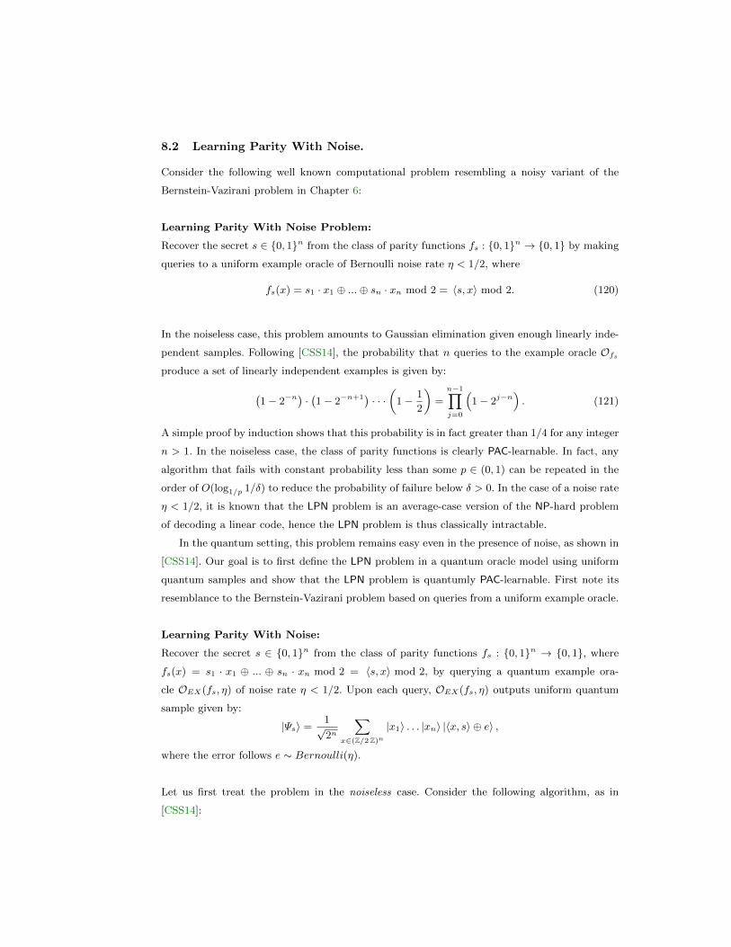
8.2 Learning Parity With Noise.
Consider the following well known computational problem resembling a noisy variant of the
Bernstein-Vazirani problem in Chapter 6:
Learning Parity With Noise Problem:
Recover the secret s ∈ 0, 1n from the class of parity functions fs : 0, 1n → 0, 1 by making
queries to a uniform example oracle of Bernoulli noise rate η < 1/2, where
fs(x) = s1 · x1 ⊕ ...⊕ sn · xn mod 2 = 〈s, x〉 mod 2. (120)
In the noiseless case, this problem amounts to Gaussian elimination given enough linearly inde-
pendent samples. Following [CSS14], the probability that n queries to the example oracle Ofsproduce a set of linearly independent examples is given by:
(1− 2−n
)·(1− 2−n+1) · · · (1− 1
2
)=
n−1∏j=0
(1− 2j−n
). (121)
A simple proof by induction shows that this probability is in fact greater than 1/4 for any integer
n > 1. In the noiseless case, the class of parity functions is clearly PAC-learnable. In fact, any
algorithm that fails with constant probability less than some p ∈ (0, 1) can be repeated in the
order of O(log1/p 1/δ) to reduce the probability of failure below δ > 0. In the case of a noise rate
η < 1/2, it is known that the LPN problem is an average-case version of the NP-hard problem
of decoding a linear code, hence the LPN problem is thus classically intractable.
In the quantum setting, this problem remains easy even in the presence of noise, as shown in
[CSS14]. Our goal is to first define the LPN problem in a quantum oracle model using uniform
quantum samples and show that the LPN problem is quantumly PAC-learnable. First note its
resemblance to the Bernstein-Vazirani problem based on queries from a uniform example oracle.
Learning Parity With Noise:
Recover the secret s ∈ 0, 1n from the class of parity functions fs : 0, 1n → 0, 1, where
fs(x) = s1 · x1 ⊕ ... ⊕ sn · xn mod 2 = 〈s, x〉 mod 2, by querying a quantum example ora-
cle OEX(fs, η) of noise rate η < 1/2. Upon each query, OEX(fs, η) outputs uniform quantum
sample given by:
|Ψs〉 =1√2n
∑x∈(Z/2 Z)n
|x1〉 . . . |xn〉 |〈x, s〉 ⊕ e〉 ,
where the error follows e ∼ Bernoulli(η).
Let us first treat the problem in the noiseless case. Consider the following algorithm, as in
[CSS14]:
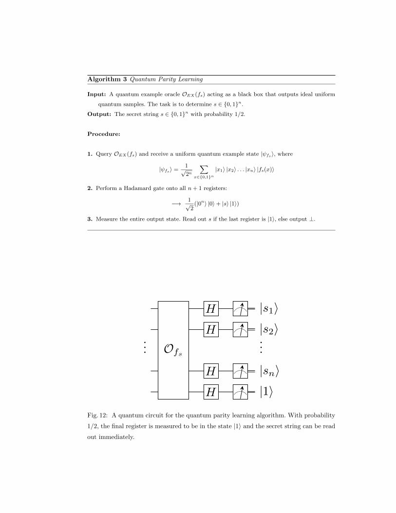
Algorithm 3 Quantum Parity Learning
Input: A quantum example oracle OEX(fs) acting as a black box that outputs ideal uniform
quantum samples. The task is to determine s ∈ 0, 1n.
Output: The secret string s ∈ 0, 1n with probability 1/2.
Procedure:
1. Query OEX(fs) and receive a uniform quantum example state |ψfs〉, where
|ψfs〉 =1√2n
∑x∈0,1n
|x1〉 |x2〉 . . . |xn〉 |fs(x)〉
2. Perform a Hadamard gate onto all n+ 1 registers:
−→ 1√2
(|0n〉 |0〉+ |s〉 |1〉)
3. Measure the entire output state. Read out s if the last register is |1〉, else output ⊥.
... Ofs
H
H
H
H
|s1〉|s2〉...
|sn〉|1〉
Fig. 12: A quantum circuit for the quantum parity learning algorithm. With probability
1/2, the final register is measured to be in the state |1〉 and the secret string can be read
out immediately.
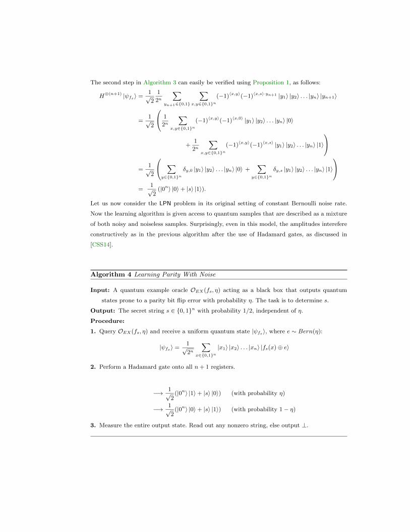
The second step in Algorithm 3 can easily be verified using Proposition 1, as follows:
H⊗(n+1) |ψfs〉 =1√2
1
2n
∑yn+1∈0,1
∑x,y∈0,1n
(−1)〈x,y〉(−1)〈x,s〉·yn+1 |y1〉 |y2〉 . . . |yn〉 |yn+1〉
=1√2
1
2n
∑x,y∈0,1n
(−1)〈x,y〉(−1)〈x,0〉 |y1〉 |y2〉 . . . |yn〉 |0〉
+1
2n
∑x,y∈0,1n
(−1)〈x,y〉(−1)〈x,s〉 |y1〉 |y2〉 . . . |yn〉 |1〉
=
1√2
∑y∈0,1n
δy,0 |y1〉 |y2〉 . . . |yn〉 |0〉 +∑
y∈0,1nδy,s |y1〉 |y2〉 . . . |yn〉 |1〉
=
1√2
(|0n〉 |0〉+ |s〉 |1〉).
Let us now consider the LPN problem in its original setting of constant Bernoulli noise rate.
Now the learning algorithm is given access to quantum samples that are described as a mixture
of both noisy and noiseless samples. Surprisingly, even in this model, the amplitudes interefere
constructively as in the previous algorithm after the use of Hadamard gates, as discussed in
[CSS14].
Algorithm 4 Learning Parity With Noise
Input: A quantum example oracle OEX(fs, η) acting as a black box that outputs quantum
states prone to a parity bit flip error with probability η. The task is to determine s.
Output: The secret string s ∈ 0, 1n with probability 1/2, independent of η.
Procedure:
1. Query OEX(fs, η) and receive a uniform quantum state |ψfs〉, where e ∼ Bern(η):
|ψfs〉 =1√2n
∑x∈0,1n
|x1〉 |x2〉 . . . |xn〉 |fs(x)⊕ e〉
2. Perform a Hadamard gate onto all n+ 1 registers.
−→ 1√2
(|0n〉 |1〉+ |s〉 |0〉) (with probability η)
−→ 1√2
(|0n〉 |0〉+ |s〉 |1〉) (with probability 1− η)
3. Measure the entire output state. Read out any nonzero string, else output ⊥.
8.3 Extended Bernstein-Vazirani Algorithm.
In this chapter, we introduce a novel qudit extension of the well known Bernstein-Vazirani prob-
lem in a computational learning setting by considering the problem over the group Z/qZ under
cyclic addition, where q is any integer. In solving this problem, we provide the basis for the LWE
problem in a quantum example oracle model.
Extended Bernstein-Vazirani Problem:
Recover the secret s ∈ (Z/qZ)n from the class of functions fs : (Z/qZ)n → Z/qZ by making
queries to a uniform example oracle for
fs(x) = s1 · x1 + ...+ sn · xn mod q = 〈s, x〉 mod q, (122)
where q is any positive integer.
Similar to the noiseless LPN problem, the classical query complexity of the above problem
is given by Ω(n). In the quantum setting, we are given a quantum example oracle Ofs and
the goal is to solve the extended Bernstein-Vazirani problem. In the following, we show that
the above problem is exactly learnable by Algorithm 5 and discuss its applications for the LWE
problem. Surprisingly, our proposed algorithm achieves a success probability in terms of Euler’s
totient function ϕ : N −→ N. Upon input q, the output ϕ(q) is defined as the number of integers
k such that gcd(k, q) = 1. Using Euler’s product formula, we can also write the probability that
Algorithm 5 succeeds as:ϕ(q)
q=
∏primes p|q
(1− 1
p
). (123)
The curious quotient ϕ(q)/q is of deep importance to number theory and has been studied for
many decades. In the 1950ies, Schinzel and Sierpinski proved that ϕ(n)/n : n = 1, 2, ... is
dense in the interval (0, 1) ⊂ R, highlighting that the ratio is highly nontrivial. Therefore, it is
not possible to find a unique limit as q approaches infinity. Euler’s product formula, Eq. (123),
gives us an intuition on how large ϕ(q)/q is, depending on the prime factorization of q. If q is
prime, we observe a simple ratio of q−1q
, hence a high probability for Algorithm 5 to succeed.
Using a result due to Rosser and Schoenfeld [RS62], we can also bound the success probability
of Algorithm 5 in the case where q > 2:5
ϕ(q)
q>
1
eγ log log(q) + 3log log(q)
, (124)
where eγ = 1.7810724... is Euler’s constant. For our purposes, this ratio is still constant and the
algorithm can be repeated to amplify the success probability as it fails with constant probability
5 In the case of q = 2, the problem is the noiseless variant of the LPN problem from Section 8.2.
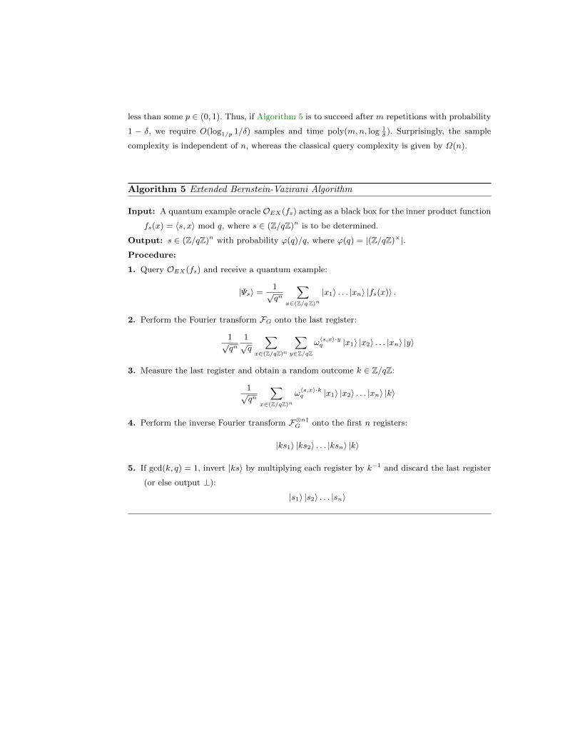
less than some p ∈ (0, 1). Thus, if Algorithm 5 is to succeed after m repetitions with probability
1 − δ, we require O(log1/p 1/δ) samples and time poly(m,n, log 1δ). Surprisingly, the sample
complexity is independent of n, whereas the classical query complexity is given by Ω(n).
Algorithm 5 Extended Bernstein-Vazirani Algorithm
Input: A quantum example oracle OEX(fs) acting as a black box for the inner product function
fs(x) = 〈s, x〉 mod q, where s ∈ (Z/qZ)n is to be determined.
Output: s ∈ (Z/qZ)n with probability ϕ(q)/q, where ϕ(q) = |(Z/qZ)×|.
Procedure:
1. Query OEX(fs) and receive a quantum example:
|Ψs〉 =1√qn
∑x∈(Z/q Z)n
|x1〉 . . . |xn〉 |fs(x)〉 .
2. Perform the Fourier transform FG onto the last register:
1√qn
1√q
∑x∈(Z/qZ)n
∑y∈Z/qZ
ω〈s,x〉·yq |x1〉 |x2〉 . . . |xn〉 |y〉
3. Measure the last register and obtain a random outcome k ∈ Z/qZ:
1√qn
∑x∈(Z/qZ)n
ω〈s,x〉·kq |x1〉 |x2〉 . . . |xn〉 |k〉
4. Perform the inverse Fourier transform F⊗n†G onto the first n registers:
|ks1〉 |ks2〉 . . . |ksn〉 |k〉
5. If gcd(k, q) = 1, invert |ks〉 by multiplying each register by k−1 and discard the last register
(or else output ⊥):
|s1〉 |s2〉 . . . |sn〉
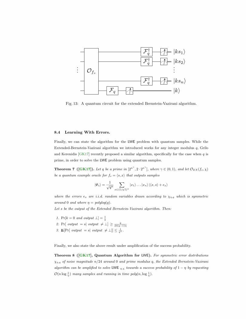
... Ofs
Fq
F†q
F†q
F†q
|ks1〉|ks2〉...
|ksn〉|k〉
Fig. 13: A quantum circuit for the extended Bernstein-Vazirani algorithm.
8.4 Learning With Errors.
Finally, we can state the algorithm for the LWE problem with quantum samples. While the
Extended-Bernstein-Vazirani algorithm we introduced works for any integer modulus q, Grilo
and Kerenidis [GK17] recently proposed a similar algorithm, specifically for the case when q is
prime, in order to solve the LWE problem using quantum samples.
Theorem 7 ([GK17]). Let q be a prime in [2nγ
, 2 · 2nγ
], where γ ∈ (0, 1), and let OEX(fs, χ)
be a quantum example oracle for fs = 〈s, x〉 that outputs samples
|Ψs〉 =1√qn
∑x∈(Z/q Z)n
|x1〉 . . . |xn〉 |〈x, s〉+ ex〉
where the errors ex are i.i.d. random variables drawn according to χη,q which is symmetric
around 0 and where η = polylog(q).
Let s be the output of the Extended Bernstein-Vazirani algorithm. Then:
1. Pr[k = 0 and output ⊥] = 1q
2. Pr[ output = s| output 6= ⊥] ≥ q24(q−1)η
3. E[Pr[ output = s| output 6= ⊥]] ≤ 1qn
.
Finally, we also state the above result under amplification of the success probability.
Theorem 8 ([GK17], Quantum Algorithm for LWE). For symmetric error distributions
χη,q of noise magnitude n/24 around 0 and prime modulus q, the Extended Bernstein-Vazirani
algorithm can be amplified to solve LWE q,χ towards a success probability of 1− η by requesting
O(n log 1η
) many samples and running in time poly(n, log 1η
).
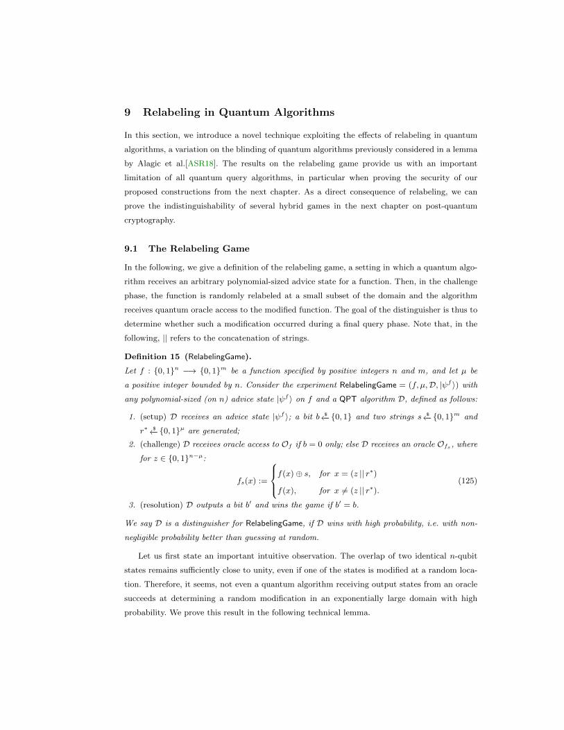
9 Relabeling in Quantum Algorithms
In this section, we introduce a novel technique exploiting the effects of relabeling in quantum
algorithms, a variation on the blinding of quantum algorithms previously considered in a lemma
by Alagic et al.[ASR18]. The results on the relabeling game provide us with an important
limitation of all quantum query algorithms, in particular when proving the security of our
proposed constructions from the next chapter. As a direct consequence of relabeling, we can
prove the indistinguishability of several hybrid games in the next chapter on post-quantum
cryptography.
9.1 The Relabeling Game
In the following, we give a definition of the relabeling game, a setting in which a quantum algo-
rithm receives an arbitrary polynomial-sized advice state for a function. Then, in the challenge
phase, the function is randomly relabeled at a small subset of the domain and the algorithm
receives quantum oracle access to the modified function. The goal of the distinguisher is thus to
determine whether such a modification occurred during a final query phase. Note that, in the
following, || refers to the concatenation of strings.
Definition 15 (RelabelingGame).
Let f : 0, 1n −→ 0, 1m be a function specified by positive integers n and m, and let µ be
a positive integer bounded by n. Consider the experiment RelabelingGame = (f, µ,D, |ψf 〉) with
any polynomial-sized (on n) advice state |ψf 〉 on f and a QPT algorithm D, defined as follows:
1. (setup) D receives an advice state |ψf 〉; a bit b $←−0, 1 and two strings s $←−0, 1m and
r∗ $←−0, 1µ are generated;
2. (challenge) D receives oracle access to Of if b = 0 only; else D receives an oracle Ofs , where
for z ∈ 0, 1n−µ:
fs(x) :=
f(x)⊕ s, for x = (z || r∗)
f(x), for x 6= (z || r∗).(125)
3. (resolution) D outputs a bit b′ and wins the game if b′ = b.
We say D is a distinguisher for RelabelingGame, if D wins with high probability, i.e. with non-
negligible probability better than guessing at random.
Let us first state an important intuitive observation. The overlap of two identical n-qubit
states remains sufficiently close to unity, even if one of the states is modified at a random loca-
tion. Therefore, it seems, not even a quantum algorithm receiving output states from an oracle
succeeds at determining a random modification in an exponentially large domain with high
probability. We prove this result in the following technical lemma.
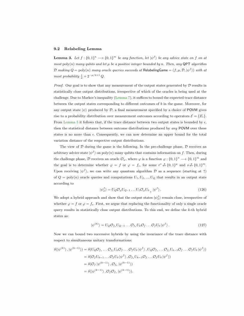
9.2 Relabeling Lemma
Lemma 3. Let f : 0, 1n −→ 0, 1m be any function, let |ψf 〉 be any advice state on f on at
most poly(n) many qubits and let µ be a positive integer bounded by n. Then, any QPT algorithm
D making Q = poly(n) many oracle queries succeeds at RelabelingGame = (f, µ,D, |ψf 〉) with at
most probability 12
+ 2−µ/4+1Q.
Proof. Our goal is to show that any measurement of the output states generated by D results in
statistically close output distributions, irrespective of which of the oracles is being used at the
challenge. Due to Markov’s inequality (Lemma 7), it suffices to bound the expected trace distance
between the output states corresponding to different outcomes of b in the game. Moreover, for
any output state |ψ〉 produced by D, a final measurement specified by a choice of POVM gives
rise to a probability distribution over measurement outcomes according to operators E = Ei.
From Lemma 5 it follows that, if the trace distance between two output states is bounded by ε,
then the statistical distance between outcome distributions produced by any POVM over these
states is no more than ε. Consequently, we can now determine an upper bound for the total
variation distance of the respective output distributions.
The view of D during the game is the following. In the pre-challenge phase, D receives an
arbitrary advice state |ψf 〉 on poly(n) many qubits that contains information on f . Then, during
the challenge phase, D receives an oracle Oϕ, where ϕ is a function ϕ : 0, 1n −→ 0, 1m and
the goal is to determine whether ϕ = f or ϕ = fs, for some r∗ $←−0, 1µ and s $←−0, 1m.
Upon receiving |ψf 〉, we can write any quantum algorithm D as a sequence (starting at ↑)
of Q = poly(n) oracle queries and computations U1, U2, ..., UQ that results in an output state
according to
|ψfϕ〉 = UQOϕUQ−1 . . . U1OϕU0↑|ψf 〉 . (126)
We adopt a hybrid approach and show that the output states |ψfϕ〉 remain close, irrespective of
whether ϕ = f or ϕ = fs. First, we argue that replacing the functionality of only a single oracle
query results in statistically close output distributions. To this end, we define the k-th hybrid
states as:
|ψ(k)〉 = UQOfsUQ−1 . . .OfsUkOf . . .OfU0 |ψf 〉 . (127)
Now we can bound two successive hybrids by using the invariance of the trace distance with
respect to simultaneous unitary transformations:
δ(|ψ(k)〉 , |ψ(k−1)〉) = δ(UQOfs . . .OfsUkOf . . .OfU0 |ψf 〉 , UQOfs . . .OfsUk−1Of . . .OfU0 |ψf 〉)
= δ(OfUk−1 . . .OfU0 |ψf 〉 ,OfsUk−1Of . . .OfU0 |ψf 〉)
= δ(Of |ψ(k−1)〉 ,Ofs |ψ(k−1)〉)
= δ(|ψ(k−1)〉 ,OfOfs |ψ(k−1)〉).
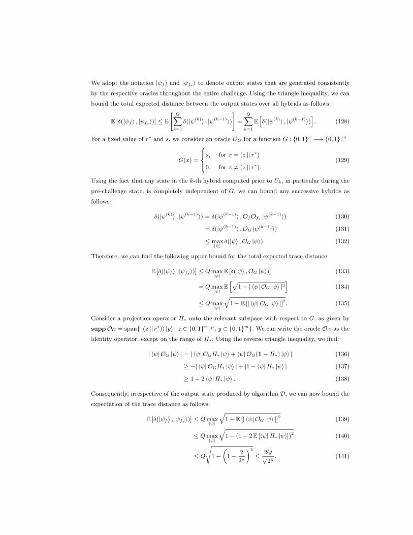
We adopt the notation |ψf 〉 and |ψfs〉 to denote output states that are generated consistently
by the respective oracles throughout the entire challenge. Using the triangle inequality, we can
bound the total expected distance between the output states over all hybrids as follows:
E [δ(|ψf 〉 , |ψfs〉)] ≤ E
[Q∑k=1
δ(|ψ(k)〉 , |ψ(k−1)〉)
]=
Q∑k=1
E[δ(|ψ(k)〉 , |ψ(k−1)〉)
]. (128)
For a fixed value of r∗ and s, we consider an oracle OG for a function G : 0, 1n −→ 0, 1,m
G(x) =
s, for x = (z || r∗)
0, for x 6= (z || r∗).(129)
Using the fact that any state in the k-th hybrid computed prior to Uk, in particular during the
pre-challenge state, is completely independent of G, we can bound any successive hybrids as
follows:
δ(|ψ(k)〉 , |ψ(k−1)〉) = δ(|ψ(k−1)〉 ,OfOfs |ψ(k−1)〉) (130)
= δ(|ψ(k−1)〉 ,OG |ψ(k−1)〉) (131)
≤ max|ψ〉
δ(|ψ〉 ,OG |ψ〉). (132)
Therefore, we can find the following upper bound for the total expected trace distance:
E [δ(|ψf 〉 , |ψfs〉)] ≤ Qmax|ψ〉
E [δ(|ψ〉 ,OG |ψ〉)] (133)
= Qmax|ψ〉
E[√
1− | 〈ψ| OG |ψ〉 |2]
(134)
≤ Qmax|ψ〉
√1− E [| 〈ψ| OG |ψ〉 |]2. (135)
Consider a projection operator Π∗ onto the relevant subspace with respect to G, as given by
suppOG = span |(z || r∗)〉 |y〉 | z ∈ 0, 1n−µ, y ∈ 0, 1m. We can write the oracle OG as the
identity operator, except on the range of Π∗. Using the reverse triangle inequality, we find:
| 〈ψ| OG |ψ〉 | = | 〈ψ| OGΠ∗ |ψ〉+ 〈ψ| OG(1−Π∗) |ψ〉 | (136)
≥ −| 〈ψ| OGΠ∗ |ψ〉 |+ |1− 〈ψ|Π∗ |ψ〉 | (137)
≥ 1− 2 〈ψ|Π∗ |ψ〉 . (138)
Consequently, irrespective of the output state produced by algorithm D, we can now bound the
expectation of the trace distance as follows:
E [δ(|ψf 〉 , |ψfs〉)] ≤ Qmax|ψ〉
√1− E [| 〈ψ| OG |ψ〉 |]2 (139)
≤ Qmax|ψ〉
√1− (1− 2E [〈ψ|Π∗ |ψ〉])2 (140)
≤ Q
√1−
(1− 2
2µ
)2
≤ 2Q√2µ. (141)
Using Markov’s inequality, we conclude that there exists a distance 2−µ/4 such that:
Prs,r∗
[δ(|ψf 〉 , |ψfs〉) ≥ 2−µ/4
]≤ 2µ/4 E [δ(|ψf 〉 , |ψfs〉)] ≤ 2−µ/4+1Q, (142)
where both the probability and the expectation are taken over all respective outcomes of sam-
pling r∗ $←−0, 1µ and s $←−0, 1m. Finally, from Lemma 5, it follows that any POVM measure-
ment of the final output states of D reveals statistically close outcome distributions:∣∣∣∣Pr[Df (1n) = 1]− Prs,r∗
[Dfs(1n) = 1]
∣∣∣∣ ≤ 2−µ/4+1Q. (143)
Finally, we can choose µ appropriately and achieve a negligible success probability.
Corollary 1. Let f : 0, 1n −→ 0, 1m be any function, let |ψf 〉 be an arbitrary advice state
on f on at most poly(n) many qubits and let µ be a super-logarithmic parameter in n. Then, any
QPT algorithm D succeeds at RelabelingGame = (f, µ,D, |ψf 〉) with at most negligible probability.
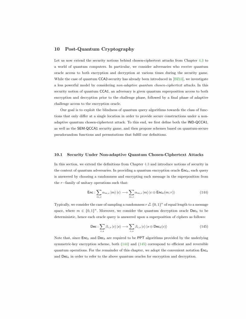
10 Post-Quantum Cryptography
Let us now extend the security notions behind chosen-ciphertext attacks from Chapter 4.3 to
a world of quantum computers. In particular, we consider adversaries who receive quantum
oracle access to both encryption and decryption at various times during the security game.
While the case of quantum CCA2-security has already been introduced in [BZ13], we investigate
a less powerful model by considering non-adaptive quantum chosen-ciphertext attacks. In this
security notion of quantum CCA1, an adversary is given quantum superposition access to both
encryption and decryption prior to the challenge phase, followed by a final phase of adaptive
challenge access to the encryption oracle.
Our goal is to exploit the blindness of quantum query algorithms towards the class of func-
tions that only differ at a single location in order to provide secure constructions under a non-
adaptive quantum chosen-ciphertext attack. To this end, we first define both the IND-QCCA1,
as well as the SEM-QCCA1 security game, and then propose schemes based on quantum-secure
pseudorandom functions and permutations that fulfill our definitions.
10.1 Security Under Non-adaptive Quantum Chosen-Ciphertext Attacks
In this section, we extend the definitions from Chapter 4.3 and introduce notions of security in
the context of quantum adversaries. In providing a quantum encryption oracle Enck, each query
is answered by choosing a randomness and encrypting each message in the superposition from
the r−family of unitary operations such that:
Enc :∑m,c
αm,c |m〉 |c〉 −→∑m,c
αm,c |m〉 |c⊕ Enck(m; r)〉 (144)
Typically, we consider the case of sampling a randomness r $←−0, 1n of equal length to a message
space, where m ∈ 0, 1n. Moreover, we consider the quantum decryption oracle Deck to be
deterministic, hence each oracle query is answered upon a superposition of ciphers as follows:
Dec :∑c,s
βc,s |c〉 |s〉 −→∑c,s
βc,s |c〉 |s⊕ Deck(c)〉 (145)
Note that, since Enck and Deck are required to be PPT algorithms provided by the underlying
symmetric-key encryption scheme, both (144) and (145) correspond to efficient and reversible
quantum operations. For the remainder of this chapter, we adopt the convenient notation Enck
and Deck in order to refer to the above quantum oracles for encryption and decryption.
Indistinguishability. We begin by first introducing a notion of indistinguishability in the
context of a quantum chosen-ciphertext attacks.
Definition 16 (IND-QCCA1).
Let Π = (KeyGen,Enc,Dec) be a symmetric-key encryption scheme and consider the IndGame
between a QPT adversary A and challenger C, defined as follows:
1. (initial phase) On input 1n, C generates a key k ← KeyGen(1n) and a bit b $←−0, 1;
2. (pre-challenge phase) A receives oracles Enck and Deck, then sends (m0,m1) to C;
3. (challenge phase) C replies with Enck(mb) and A receives an oracle for Enck only;
4. (resolution phase) A outputs a bit b′, and wins if b = b′.
We say Π has indistinguishable encryptions under non-adaptive quantum chosen-ciphertext at-
tack (or is IND-QCCA1-secure) if, for every QPT A, there exists a negligible function ε(n) such
that: Pr[A wins IndGame] ≤ 1/2 + ε(n).
Semantic Security. In this section, we first introduce semantic security under a QCCA1
learning phase and then prove an important equivalence between our notion of indistinguisha-
bility and semantic security.
Definition 17 (SEM-QCCA1). Let Π = (KeyGen,Enc,Dec) be an encryption scheme, and con-
sider the experiment SemGame with a QPT A, defined as follows.
1. (initial phase) A key k ← KeyGen(1n) and bit b $←−0, 1 are generated;
2. (pre-challenge phase) A receives access to oracles Enck and Deck, then outputs a classical
challenge template consisting of (Samp, h, f);
3. (challenge phase) A plaintext m ← Samp is generated; A receives h(m) and an oracle for
Enck only; if b = 1, A also receives Enck(m).
4. (resolution) A outputs a string s, and wins if s = f(m).
We say Π is semantically secure under non-adaptive quantum chosen ciphertext attack (or is
SEM-QCCA1) if, for every QPT A, there exists a QPT S such that the challenge templates output
by A and S are identically distributed, and there exists a negligible function ε(n) such that:∣∣∣∣∣ Prk
$←−K[A(1n,Enck(m), h(m)) = f(m)] − Pr[S(1n, |m|, h(m)) = f(m)]
∣∣∣∣∣ ≤ ε(n),
where, in both cases, the probability is taken over plaintexts m← Samp.
Equivalence of Indistinguishability and Semantic Security. Let us now show the
equivalence of the new security notions we introduced in this chapter. In the following, we
provide a standard proof, following related approaches in [GHS16].
Theorem 9. Let Π = (KeyGen,Enc,Dec) be a symmetric-key encryption scheme. Then, Π is
IND-QCCA1-secure if and only if Π is SEM-QCCA1-secure.
Proof. Suppose Π is IND-QCCA1-secure, i.e. has indistinguishable encryptions. Let A be a QPT
algorithm against SEM that receives a challenge Enck(m). Define a QPT simulator S that also
challenges SEM but simply runs A as a subroutine as follows: Instead of receiving Enck(m)
during the SEM challenge, S relies only on the side information h(m), in particular the plaintext
length |m|, and simulates A’s encryption and decryption oracles by making use of its own QCCA1
learning phase. At the challenge phase, S simply encrypts the string 1|m| and forwards Enck(1|m|)
to A. After another emulated learning phase, S finally outputs the same target f(m) that A
outputs. Since Π has indistuinguishable encryptions by assumption, A’s success probability
must be negligibly close to the original SEM game of S.
Now, suppose Π is not IND-QCCA1-secure, hence there exists a QPT distinguisher A against
IND-QCCA1-security. This allows us to build a distinguisher D running A as a subroutine against
the SEM security game as follows: By using its oracles from the QCCA1 learning phases, D
simulates the IND-QCCA1 security game of A by simply forwarding all queries to its own oracles.
At the QIND challenge phase, A prepares two messages (m0,m1) and presents them to D. Then,
D prepares a SEM challenge template (U, h, f), where U describes the uniform distribution over
plaintexts m0,m1, the side information is given by the length of the messages and where the
target function f(m) concerns the function that distinguishes between m0 and m1, i.e. f(m0) = 0
and f(m1) = 1. Using this SEM template, D receives a ciphertext Enck(m) and presents it to
A as an IND-QCCA1 challenge. Finally, D simply outputs whatever target bit A outputs. By
assumption, A succeeds with nonnegligible probability and therefore D breaks the SEM-QCCA1
security game.
10.2 Quantum-secure Pseudorandom Functions and Permutations
In order to find constructions for quantum-secure symmetric-key cryptography, we require the
use of appropriate building blocks. Let us now extend the concept of secure pseudorandom func-
tions from Chapter 4.4 to a setting in which an adversary in possession of a quantum computer
can query the function on a superposition of inputs. Remarkably, one can find quantum-secure
constructions for pseudorandom functions that are secure in this model. Moreover, as shown
by Zhandry [Zha12], one can construct quantum-secure PRF’s either from the assumption that
LWE is hard with classical samples or from the existence of quantum one-way functions.
Definition 18 (Quantum-secure Pseudorandom Function).
Let fkk∈K be a family of pseudorandom functions on a key-space K, a domain X and a range
Y. QPRF = fkk∈K is a function family of quantum-secure pseudorandom functions if (for
every choice of key k) fk looks indistinguishable from a perfectly random function, hence if, for
every QPT distinguisher D, there exists a negligible function ε(n) such that:∣∣∣∣∣ Prk
$←−K[D|fk〉(1n) = 1] − Pr
f$←− F:X→Y
[D|f〉(1n) = 1]
∣∣∣∣∣ ≤ ε(n) (146)
A special variant of pseudorandom functions is realized in keyed permutations on strings,
which can be obtained directly from purely standard assumptions on the existence of one-way
functions [Zha16]. We distinguish between quantum-secure and strong quantum-secure pseudo-
random permutations.
Definition 19 (Quantum-secure Pseudorandom Permutation).
Let πkk∈K be a family of keyed permutations operating on bit strings of domain X upon a key-
space K. QPRP = πkk∈K is a funcion family of quantum-secure pseudorandom permutations
if (for every choice of key k) πk looks indistinguishable from a random permutation on strings
in X , hence if, for every QPT distinguisher D, there exists a negligible function ε(n) such that:∣∣∣∣∣ Prk
$←−K[D|πk〉(1n) = 1] − Pr
π$←− SX
[D|π〉(1n) = 1]
∣∣∣∣∣ ≤ ε(n), (147)
where SX denotes the set of all permutations over strings in X .
In order to realize security under a quantum chosen-ciphertext attack, we require an even
stronger notion of pseudorandomness, in particular in the presence of a decryption oracle. For-
tunately, there exist constructions for the following standard, as considered in [Zha16].
Definition 20 (Strong Quantum-secure Pseudorandom Permutation).
A family of pseudorandom permutations πkk∈K is a function family of strong quantum-secure
pseudorandom permutations QPRP if πk together with its inverse permutation π−1k look indis-
tinguishable from a random permutation, hence if, for every QPT distinguisher D, there exists
a negligible function ε(n) such that:∣∣∣∣∣ Prk
$←−K[D|πk〉|π
−1k〉(1n) = 1] − Pr
π$←− SX
[D|π〉|π−1〉(1n) = 1]
∣∣∣∣∣ ≤ ε(n). (148)
Finally, we provide schemes based on the above building blocks of pseudorandom functions
and permutations that are quantumly secure under a quantum-chosen ciphertext attack we
introduced in this thesis.
10.3 Secure Constructions
We consider the PRF scheme in Construction 1 and show that it is secure under a non-adaptive
quantum chosen-ciphertext attack. The intuition is that, once the pseudorandom function is
taken to be quantum-secure, the pre-challenge phase reveals at most a polynomial amount of
evaluations of the pseudorandom function, despite the presence of a decryption oracle. Note
that, in this scheme, the encryption oracle only reveals a single functional evaluation of the PRF
at a random location at a time, while the decryption oracle can additionally serve as a quantum
oracle for the function of the underlying encryption scheme. In fact, the adversary can generate
superposition queries to a PRF fk over the entire input space by simply initializing both the
ciphertext and plaintext register to the all-zero state and preparing a superposition over the
random register:
Deck :∑
τ∈0,1nβτ |0〉 |τ〉 |0〉 −→
∑τ∈0,1n
βτ |0〉 |τ〉 |fk(τ)〉 . (149)
At first sight, however, it is not clear whether being able to generate superpositions gives the
adversary additional power during the challenge phase. Therefore, we have to bound the amount
of information that quantum query algorithms can learn in a suitable way. Our contribution is
to show that this advantage is still negligible and that Construction 1 has indistinguishable
encryptions, even in the presence of decryption oracles under a non-adaptive quantum chosen-
ciphertext attack. Finally, due to the equivalence results from the previous section, our proposed
scheme then also satisfies indistinguishability of encryptions and semantic security.
Theorem 10. Let QPRF be a family of quantum-secure pseudorandom functions. Then, the
scheme Π = (KeyGen,Enc,Dec) from Construction 1 is IND-QCCA1-secure.
Proof. Our goal is to show that any QPT adversary A wins IndGame. under a QCCA1 learning
phase with at most negligible probability. To this end, we introduce a sequence of indistinguish-
able hybrid games until we arrive at a security game in which the challenge is perfectly hidden
and the adversary cannot win. Let us sketch the proof.
First, we replace the QPRF from the standard security game with a perfectly random func-
tion. According to QPRF security, we only negligibly affect the overall success probability of the
adversary. In the IND-CCA1 model in which the adversary is classical, this hybrid already com-
pletes the proof, as the probability of observing the same randomness outside of the challenge
is negligible. However, since the adversary in the quantum model is allowed to issue quantum
queries, the previous observation does not translate directly to a QPT adversary who can eval-
uate the function in superposition over the entire input space.
Therefore, we introduce a final hybrid game and relabel the challenge value of the function
uniformly at random. For the remainder of the game, we respond to encryption queries with
the same function, now modified at a single location. Due to Corollary 1, no QPT algorithm
can distinguish between these two hybrids, else it would imply a successful distinguisher against
RelabelingGame.
With this in mind, we consider the following sequence of indistinguishable hybrid games:
Game 0: The adversary is playing the standard IndGame for the scheme Π. In the pre-challenge
phase, the adversary receives oracles Enck and Deck, whereas in the challenge phase, oracle
access is restricted to Enck only. A challenge ciphertext (r∗, fk(r∗) ⊕mb) is produced and
the goal of the adversary is to output a bit b′ = b.
Game 1: The QPRF fk from the previous scheme is replaced by a perfectly random function
f throughout the entire security game.
Game 2: If a challenge ciphertext is generated using a randomness already known to the ad-
versary from the pre-challenge phase, the game is aborted and the adversary wins.
Game 3: Until the challenge phase, the security game takes place as in the previous hybrid. At
the start of the next phase, the challenge value of the function is replaced by f(r∗)⊕s, where
s is a uniformly random string s $←−0, 1n. For the remainder of the game, all encryption
queries are answered using the function
fs(x) =
f(r∗)⊕ s, for x = r∗
f(x), for x 6= r∗.(150)
Suppose there exists a QPT adversary A that wins Game 0 with nonnegligible probability, hence
there exists some polynomial p(n) such that:
Pr[A wins IndGame] ≥ 1/2 + 1/p(n). (151)
Our claim is that the same adversary must (up to at most negligible probability) also succeed
at Game 3 in which the challenge is perfectly hidden by means of a hybrid argument.
Game 0 vs. Game 1:
Since we assumed the PRF fk to be quantum-secure, we can replace it with a perfectly random
function and only negligibly affect the success probability in Eq.(151). Note that an adversary
A that succeeds at Game 0 but not at Game 1 (i.e. A only wins with at most negligible
probability), allows us to build an fk−distinguisher that violates QPRF security. We can verify
this fact, as follows. Let D be the distinguisher that is given quantum oracle access Oϕ to a
function ϕ : 0, 1n −→ 0, 1n, and the goal is to output 0, whenever ϕ is a perfectly random
function, and to output 1, if ϕ = fk for some k. Let D now proceed as follows. It simulates the
IND-QCCA1 security game of A by responding to quantum queries using oracles Encϕ and Decϕ
that can be implemented based on the output of Oϕ. If A wins IndGame and outputs b′ = b,
then D outputs 1, else D outputs 0 otherwise. Moreover, since A succeeds with nonnegligible
probability in Game 0, so does the distinguisher D, and for infinitely many n:∣∣∣∣∣ Prk
$←− 0,1n[D|fk〉(1n) = 1] − Pr
f$←− F:X→Y
[D|f〉(1n) = 1]
∣∣∣∣∣ ≥ 1/p(n)− ε(n).
Therefore, our crucial assumption of QPRF security is broken by this distinguisher and we
conclude that A must also win Game 1 with nonnegligible probability.
Game 1 vs. Game 2:
In this hybrid, a fresh randomness is guaranteed for each encryption, else the game is aborted.
As the probability of sampling the same randomness twice is negligible, the difference between
these two games is only negligible with respect to the overall success probability in the security
game.
Game 2 vs. Game 3:
Any quantum adversary against the IND-QCCA1 security game can be separated into a pre-
challenge quantum query routine, as well as final challenge routine. We can describe the QPT
adversary A from Game 2 as follows. Upon an initial state A performs T = poly(n) unitary
computations U1, U2, ..., UT and alternating queries to the encryption and decryption oracle,
and outputs:
|Ψf 〉 = UTODecUT−1OEncUT−2 . . . U2ODecU1OEncU0 |Ψ0〉 . (152)
In the challenge phase, A continues to perform encryption oracle queries with respect to f , as
well as final unitary computations UQ+1, UQ+2, ..., UQ upon |Ψf 〉, and generates:
|Ψff 〉 = UQOEncUQ−1 . . . UT+2OEncUT+1 |Ψf 〉 , (153)
Finally, after completing both routines, A measures the final output state and outputs b′. Sup-
pose now that the adversary A succeeds at Game 2 but not at Game 3, i.e. A only wins with at
most negligible probability. We argue that the same adversary serves as a distinguisher against
RelabelingGame, hence must violate Corollary 1.
Let D be a QPT adversary against RelabelingGame that receives a polynomial-sized advice
state on f (such as a classical circuit description) that allows for the implementation of Of .
D now proceed as follows. It simulates the IND-QCCA1 security game of A by responding to
quantum queries using oracles Encf and Decf that can be implemented based on the output of
Of . Consequently, D can emulate any query sequence in Eq.(152) during the security game. In
the challenge phase, D receives a quantum oracle Oϕ for a function ϕ : 0, 1n −→ 0, 1n, whose
goal is to output 0, whenever ϕ is a perfectly random function, and to output 1, if ϕ = fs for
some x∗ $←−0, 1n and s $←−0, 1n. Similarly, D can respond to encryption queries by emulating
an oracle Encϕ based on the output of Oϕ. If A wins the IndGame game and outputs b′ = b,
then D outputs 1, else D outputs 0. Since A succeeds with nonnegligible probability in Game
2, so does the distinguisher D, and for infinitely many n:∣∣∣∣∣Pr[D|f〉(1n) = 1]− Prs,r∗
$←− 0,1n[D|fs〉(1n) = 1]
∣∣∣∣∣ ≥ 1/p(n)− ε(n). (154)
Consequently, we conclude that A must also win Game 3 with nonnegligible probability, else A
would imply the existence of a distinguisher against RelabelingGame, thus violate Corollary 1.
Since the challenge ciphertext in Game 3 is given by (r∗, f(r∗) ⊕ s ⊕ mb), the IndGame
challenge now amounts to an information-theoretically secure one-time pad, hence the impossible
task of distinguishing between two uniformly random strings. Therefore, since the view of A
is indistinguishable from such a challenge of perfect secrecy, we must now arrive at an overall
contradiction and conclude that no such QPT algorithm A with nonnegligible success probability
exists. In summary, we must conclude that for any QPT adverdary A playing the IND-QCCA1
game:
Pr[A wins IndGame] ≤ 1
2+ ε(n). (155)
Finally, as a direct consequence of the equivalance results of Section 10.1, let us conclude the
previous result with the following additional observation:
Corollary 2. Let QPRF be a function family of quantum-secure pseudorandom functions. Then,
Π = (KeyGen,Enc,Dec) from Construction 1 is SEM-QCCA1-secure.
It is well known, see for example [KL15], that the PRF scheme is easily malleable by an adversary
with adaptive decryption oracle access in a CCA2 learning phase. Therefore, Construction 1 is
neither secure under classical nor quantum adaptive chosen-ciphertext attacks.
Finally, we provide another symmetric-key encryption scheme based on pseudorandom per-
mutations that recently appeared in work by Gagliardoni et al. [GHS16]. As for the previous
construction, we follow a similar proof and introduce indistinguishable hybrids and a blinding
argument.
Construction 3. Consider a family of keyed permutations πkk∈K operating on bit strings of
length 2n, where n is a security parameter and K = 0, 1n is a key space. Define a symmetric-
key encryption scheme Π = (KeyGen,Enc,Dec) as follows:
1. (key generation) KeyGen: on input 1n, generate a key k $←−0, 1n;
2. (encryption) Enck: on message m ∈ 0, 1n, choose a randomness r $←−0, 1n and output
Enck(m; r) = πk(m||r);
3. (decryption) Deck: on cipher c ∈ 0, 12n, output the first n bits of the string produced by
Deck(c) = π−1k (c)1,...,n = (m || r)1,...,n = m;
4. (correctness) (Deck Enck)(m; r) = (π−1k (πk(m||r)))1,...,n = m.
Let us now consider the security under a non-adaptive quantum chosen-ciphertext attack. Again,
the intuition is that, once the strong pseudorandom permutation is taken to be quantum-secure,
the pre-challenge phase reveals at most a polynomial amount of evaluations of the pseudorandom
permutation, despite the presence of a decryption oracle for the permutation and its inverse.
Therefore, no adaptive access to a quantum encryption oracle is sufficient to succeed at the
challenge.
Theorem 11. Let QPRP be a family of strong pseudorandom permutations. Then, the scheme
Π = (KeyGen,Enc,Dec) from Construction 3 is IND-QCCA1-secure.
Proof. As in the previous construction, our goal is to show that any QPT adversary A wins
the IND-QCCA1 security game with at most negligible probability. We introduce a sequence
of indistinguishable hybrid games until we arrive at a security game in which the challenge is
perfectly hidden through relabeling and the adversary cannot win. Let us first sketch the proof.
First, we replace the strong QPRP from the original security game with a perfectly random
permutation operating on bit strings of length 2n. According to QPRP security, we only neg-
ligibly affect the overall success probability. Next, we introduce a hybrid that guarantees fresh
randomness for each encryption, else we abort the game. Finally, we introduce a hybrid game
in which we relabel challenge values of the permutation uniformly at random on a negligible
subset of the domain. For the remainder of the game, we respond to encryption queries with the
same modified function. Due to Corollary 1, no QPT algorithm can distinguish between these
two hybrids, else it would imply a successful distinguisher against RelabelingGame.
Consider the following sequence of indistinguishable hybrid games:
Game 0: The adversary is playing the standard IndGame for the scheme Π. In the pre-challenge
phase, the adversary receives oracles Enck and Deck, whereas in the challenge phase, oracle
access is restricted to Enck only. A challenge ciphertext πk(mb||r∗) is produced and the goal
of the adversary is to output a bit b′ = b.
Game 1: The QPRP πk is replaced by a random permutation π ∈ S2n.
Game 2: Fresh randomness is guaranteed for each new encryption, else the game is aborted
and the adversary wins.
Game 3: At the beginning of the challenge phase, the permutation is relabeled upon all strings
corresponding to the challenge randomness. For a uniformly random string s $←−0, 12n, all
encryption queries during the challenge phase are now answered with
πs(x) =
π(x)⊕ s, for x = (z || r∗)
π(x), for x 6= (z || r∗).(156)
Suppose there exists a QPT adversary A that wins Game 0 with nonnegligible probability,
hence there exists some polynomial p(n) such that:
Pr[A outputs b′ = b] ≥ 1/2 + 1/p(n). (157)
As before, our claim is that the same adversary must (up to at most negligible probability) also
succeed at Game 3 in which the challenge is perfectly hidden by means of a hybrid argument.
Game 0 vs. Game 1:
Since we assumed the strong QPRP πk to be quantum-secure, we can replace it with a random
permutation π on the bit strings of length 2n and only negligibly affect the success probability
in Eq.(157). Note that an adversary A that succeeds at Game 0 but not at Game 1 (i.e. A only
wins with at most negligible probability), allows us to build a πk−distinguisher that violates
QPRP security when receiving quantum oracle access to Oϕ and Oϕ−1 , where ϕ is a function
ϕ : 0, 12n −→ 0, 12n. As in the previous proof, we can construct a distinguisher D by running
A such that for infinitely many n:∣∣∣∣∣ Prk
$←− 0,1n[D|πk〉|π
−1k〉(1n) = 1] − Pr
π$←− S2n
[D|π〉|π−1〉(1n) = 1]
∣∣∣∣∣ ≥ 1/p(n)− ε(n). (158)
Therefore, our crucial assumption of strong QPRP security is broken by this distinguisher and
we conclude that A must also win Game 1 with nonnegligible probability.
Game 1 vs. Game 2:
In this hybrid, a fresh randomness is guaranteed for each encryption, else the game is aborted.
As the probability of sampling the same randomness twice is negligible, the difference between
these two games is only negligible with respect to the overall success probability in the security
game.
Game 2 vs. Game 3:
Any quantum adversary against the IND-QCCA1 security game can be separated into a pre-
challenge quantum query routine, as well as final challenge routine. We can describe the QPT
adversary A from Game 2 as follows. Upon an initial state A performs T = poly(n) unitary
computations U1, U2, ..., UT and alternating queries to the encryption and decryption oracle,
and outputs:
|Ψπ〉 = UQODecUQ−1OEncUQ−2 . . . U2ODecU1OEncU0 |Ψ0〉 . (159)
In the challenge phase, A applies final encryption and decryption oracle queries with respect
to π, as well as Q = poly(n) final unitary computations UQ+1, UQ+2, ..., UQ upon |Ψπ〉, and
generates:
|Ψππ 〉 = UQODecUQ−1OEncUQ−2 . . . U2ODecU1OEncUQ+1 |Ψπ〉 , (160)
Finally, after completing both routines, A measures the output state and outputs b′. Suppose
now that the adversary A succeeds at Game 2 but not at Game 3, i.e. A only wins with at
most negligible probability. We will show that the same adversary must win RelabelingGame,
thus must violate Corollary 1.
Let D be a QPT adversary against RelabelingGame that receives a polynomial-sized advice
state on π (such as a classical circuit description) that allows for the implementation of Oπ and
Oπ−1 . D now proceed as follows. It simulates the IND-QCCA1 security game of A by responding
to quantum queries using oracles Encπ and Decπ that can be implemented based on the output
of Oπ and Oπ−1 . Consequently, D can emulate any query sequence in Eq.(159) during the
security game. Next, in the challenge phase of RelabelingGame, D receives oracle access to Oϕ,
where ϕ : 0, 12n −→ 0, 12n, and the goal is to output 0, whenever ϕ is a perfectly random
permutation and to output 1, if ϕ = πs for some r∗ $←−0, 1n and s $←−0, 12n. Similarly, D can
respond to encryption queries by emulating an oracle Encϕ based on the output of Oϕ. If A wins
the IND-QCCA1 and outputs b′ = b, then D outputs 1, else D outputs 0. Since we assumed that
A succeeds with nonnegligible probability in Game 2, so must D, and for infinitely many n:∣∣∣∣Prs,r∗
[D|πs〉(1n) = 1] − Pr[D|π〉(1n) = 1]
∣∣∣∣ ≥ 1/p(n)− ε(n). (161)
Therefore, we conclude that A must also win Game 3 with nonnegligible probability, in violation
of Corollary 1.
As in the previous proof, the IndGame challenge now amounts to the impossible task of
distinguishing between two uniformly random strings. Therefore, since the view of A is indistin-
guishable from such a challenge of perfect secrecy, we must now arrive at an overall contradiction
and conclude that no such QPT algorithm A with nonnegligible success probability exists. In
summary, we must conclude that for any QPT adverdary A playing the IND-QCCA1 game:
Pr[A wins IndGame] ≤ 1
2+ ε(n). (162)
Consequently, again as a direct consequence of the equivalance between IND-QCCA1 and
SEM-QCCA1, we can conclude the previous result with the following additional observation:
Corollary 3. Let QPRP be a function family of quantum-secure pseudorandom permutations.
Then, the scheme Π = (KeyGen,Enc,Dec) from Construction 3 is both IND-QCCA1-secure, as
well as SEM-QCCA1-secure.
11 The Physical Realization of Quantum Computation
The simulation of quantum systems turns out to scale surprisingly poorly on conventional clas-
sical computers. In order to simulate N spin 1/2 particles and to solve the Schrodinger equation,
one needs to store vectors of size 2N , as well as manipulate matrices of size 2N × 2N . Due to
this exponential scaling, it is well known that classical computers are highly inefficient in simu-
lating the dynamics of quantum systems. This fact has already puzzled physicists in the 1980s,
who hypothesized that an intrinsically quantum mechanical computer could potentially be more
suitable for these tasks. In fact, it is often attributed to Richard Feynman [Fey82] to have been
the first to speculate on the possibility of building quantum computers. The prospect of building
a computer that would outperform any classical computing architecture and efficiently simu-
late quantum physics seemed captivating. In 1989, David Deutsch gave the first example of a
quantum algorithm for a black box problem which could be solved faster with quantum me-
chanical means than with classical ones [Deu89]. Perhaps most notably, it was Peter Shor’s 1994
discovery of efficient quantum algorithms for the factoring of integers and computing discrete
logarithms [Sho94] that truly drew the attention towards the field of quantum computation.
Only a few years later, Ignacio Cirac and Peter Zoller proposed a physical system of trapped
ions on which quantum information processing could be realized [CZ95]. In this architecture,
single trapped ions are engineered to carry quantum information and are both manipulated and
measured with focused laser beams. Already within a year’s time, David Wineland’s group at
National Institute of Standards and Technology achieved a breakthrough in ion-trap quantum
computers [MMKW99], namely a controlled bit flip on a single ion. This experiment is often
considered as the birth of experimental quantum computation. In this chapter, we give a ba-
sic introduction to trapped-ion quantum computers. To this end, we follow an excellent survey
on trapped-ion computation by Haffner and Blatt [HRB08]. In later sections, we also describe
recent implementations of quantum algorithms and further advances in the field.
11.1 DiVincenzo Criteria
All quantum information processing is concerned with the storage and coherent manipulation of
information in a quantum system. In the previous chapters, we showed how quantum computers
could solve certain mathematical problems faster than classical computers using the principles
of quantum mechanics. In order to harness this quantum speed-up, however, one has to realize
quantum computation in a physical system. Fortunately, nature presents us with many possible
ways of realizing a qubit in a physical system. As typical representations of a qubit are found in
the two states of a spin 1/2 particle, the vertical or horizontal polarization of a photon or simply
the ground and excited states of an atom, each representation comes with its own drawbacks
and advantages. While photons are easy to generate, they have proven to be difficult to interact
on the basis of nonlinear materials alone [NC10]. Similarly, both the observation and control
of spin states poses great difficulty, unless a carefully engineered environment is achieved. An
example of such circumstances is realized in a trapped-ion quantum computer, where ions are
confined in a potential trap and subsequently cooled.
In 1996, David DiVincenzo, at the IBM Thomas J. Watson Research Center, proposed the
following list of guidelines for a successful physical implementation of a quantum computer:
[DiV00]
1. A scalable physical system with well characterized qubits.
2. The ability to initialize the state of the qubits to a simple initial state.
3. Long relevant decoherence times, much longer than the gate operation time.
4. A universal set of quantum gates.
5. A qubit-specific measurement capability.
Having the possibility of a functioning interface between quantum computers and devices for
quantum communication in mind, DiVincenzo also added two additional requirements:
6. The ability to interconvert stationary and flying qubits.
7. The ability to faithfully transmit flying qubits between specified locations.
Currently, the trapped-ion computer is oftentimes regarded as the leading quantum computing
architecture, while the runner-up technology is believed to be that of the solid-state architecture
of superconducting qubits [LMRD17]. In this thesis, we present the ion-trap quantum computer
as a model for quantum computation and discuss its fundamental properties and capabilities.
When performing quantum information processing, such as the algorithms from the previous
chapters, the ability to coherently manipulate as well as store information with low rates of error
is crucial. Decoherence of quantum systems poses enormous difficulty to both of these tasks.
In the next section, we will outline the extent to which trapped ion computation satisfies these
criteria.
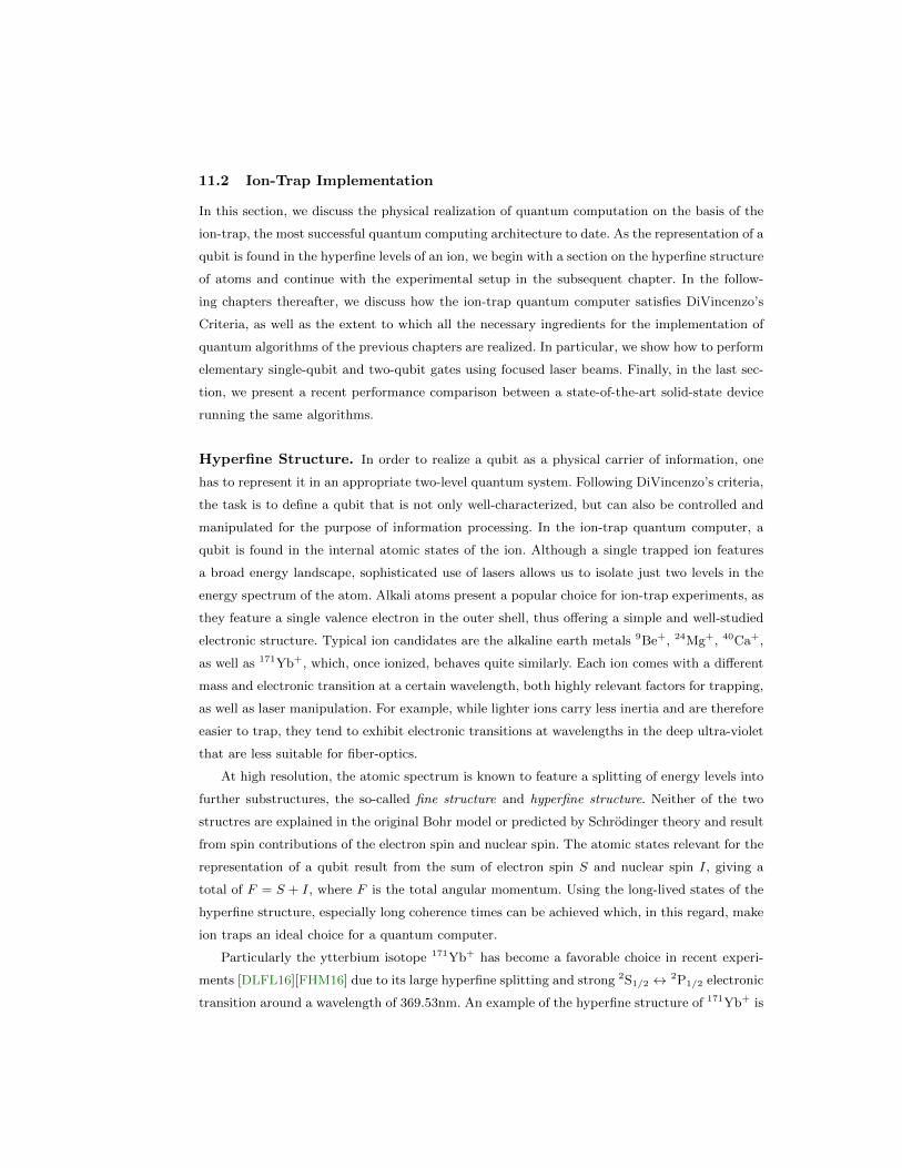
11.2 Ion-Trap Implementation
In this section, we discuss the physical realization of quantum computation on the basis of the
ion-trap, the most successful quantum computing architecture to date. As the representation of a
qubit is found in the hyperfine levels of an ion, we begin with a section on the hyperfine structure
of atoms and continue with the experimental setup in the subsequent chapter. In the follow-
ing chapters thereafter, we discuss how the ion-trap quantum computer satisfies DiVincenzo’s
Criteria, as well as the extent to which all the necessary ingredients for the implementation of
quantum algorithms of the previous chapters are realized. In particular, we show how to perform
elementary single-qubit and two-qubit gates using focused laser beams. Finally, in the last sec-
tion, we present a recent performance comparison between a state-of-the-art solid-state device
running the same algorithms.
Hyperfine Structure. In order to realize a qubit as a physical carrier of information, one
has to represent it in an appropriate two-level quantum system. Following DiVincenzo’s criteria,
the task is to define a qubit that is not only well-characterized, but can also be controlled and
manipulated for the purpose of information processing. In the ion-trap quantum computer, a
qubit is found in the internal atomic states of the ion. Although a single trapped ion features
a broad energy landscape, sophisticated use of lasers allows us to isolate just two levels in the
energy spectrum of the atom. Alkali atoms present a popular choice for ion-trap experiments, as
they feature a single valence electron in the outer shell, thus offering a simple and well-studied
electronic structure. Typical ion candidates are the alkaline earth metals 9Be+, 24Mg+, 40Ca+,
as well as 171Yb+, which, once ionized, behaves quite similarly. Each ion comes with a different
mass and electronic transition at a certain wavelength, both highly relevant factors for trapping,
as well as laser manipulation. For example, while lighter ions carry less inertia and are therefore
easier to trap, they tend to exhibit electronic transitions at wavelengths in the deep ultra-violet
that are less suitable for fiber-optics.
At high resolution, the atomic spectrum is known to feature a splitting of energy levels into
further substructures, the so-called fine structure and hyperfine structure. Neither of the two
structres are explained in the original Bohr model or predicted by Schrodinger theory and result
from spin contributions of the electron spin and nuclear spin. The atomic states relevant for the
representation of a qubit result from the sum of electron spin S and nuclear spin I, giving a
total of F = S + I, where F is the total angular momentum. Using the long-lived states of the
hyperfine structure, especially long coherence times can be achieved which, in this regard, make
ion traps an ideal choice for a quantum computer.
Particularly the ytterbium isotope 171Yb+ has become a favorable choice in recent experi-
ments [DLFL16][FHM16] due to its large hyperfine splitting and strong 2S1/2 ↔ 2P1/2 electronic
transition around a wavelength of 369.53nm. An example of the hyperfine structure of 171Yb+ is
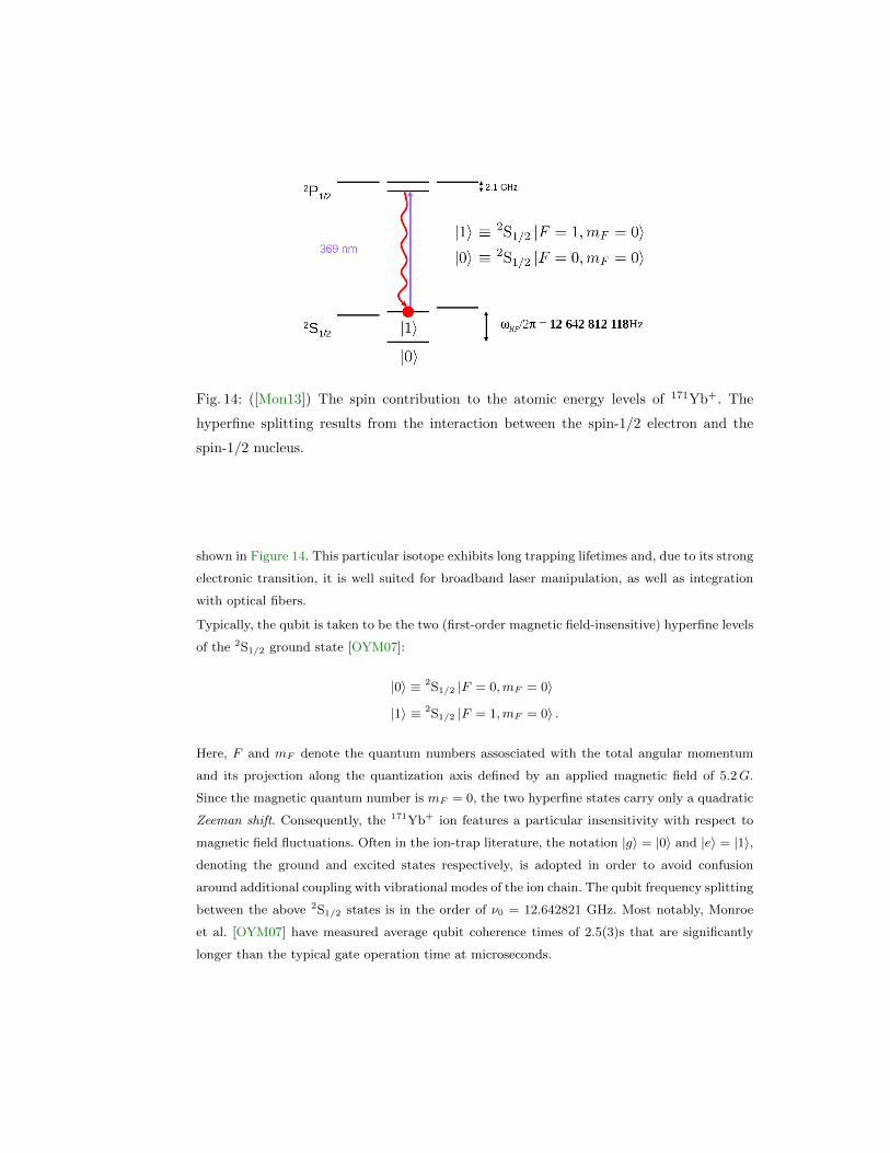
Fig. 14: ([Mon13]) The spin contribution to the atomic energy levels of 171Yb+. The
hyperfine splitting results from the interaction between the spin-1/2 electron and the
spin-1/2 nucleus.
shown in Figure 14. This particular isotope exhibits long trapping lifetimes and, due to its strong
electronic transition, it is well suited for broadband laser manipulation, as well as integration
with optical fibers.
Typically, the qubit is taken to be the two (first-order magnetic field-insensitive) hyperfine levels
of the 2S1/2 ground state [OYM07]:
|0〉 ≡ 2S1/2 |F = 0,mF = 0〉
|1〉 ≡ 2S1/2 |F = 1,mF = 0〉 .
Here, F and mF denote the quantum numbers assosciated with the total angular momentum
and its projection along the quantization axis defined by an applied magnetic field of 5.2G.
Since the magnetic quantum number is mF = 0, the two hyperfine states carry only a quadratic
Zeeman shift. Consequently, the 171Yb+ ion features a particular insensitivity with respect to
magnetic field fluctuations. Often in the ion-trap literature, the notation |g〉 = |0〉 and |e〉 = |1〉,
denoting the ground and excited states respectively, is adopted in order to avoid confusion
around additional coupling with vibrational modes of the ion chain. The qubit frequency splitting
between the above 2S1/2 states is in the order of ν0 = 12.642821 GHz. Most notably, Monroe
et al. [OYM07] have measured average qubit coherence times of 2.5(3)s that are significantly
longer than the typical gate operation time at microseconds.
Fig. 15: ([Mon13]) The University of Maryland ion-trap at the Chris Monroe lab, 2013.
Each dot represents a single 171Yb+ ion exhibiting state dependent fluorescence when
driven by individual focused laser beams. A CCD camera collects fluorescence from the
scattering of photons and creates an image over thousands of measurements.
Experimental Setup. The main component of an ion-trap quantum computer is an elec-
tromagnetic trap, a vacuum chamber surrounded by four cylindrical electrodes. In order to
produce the necessary trapping potential towards axial confinement of the ions, the end caps
of the rods are biased at different voltages. However, as we will show now, trapping ions by
means of static electric fields alone is not possible. Earnshaw’s theorem states that a charged
particle cannot be confined in three dimensions by static electric fields, as the divergence of the
field vanishes in empty space. This fact can easily be verified in the following short argument.
Let r0 = (x0, y0, z0) denote the coordinates of the charge. Then, for any trapping potential, we
require that the particle returns to its equilibrium position once it is displaced. Consequently,
we demand from the potential energy U(r) that:
∇U(r0) = 0, ∇2U(r0) > 0. (163)
However, since the electric potential energy is given by U(r) = q Φ(r), where Φ is the electrostatic
potential, we must conclude from Gauss’ law that:
∇2U(r) = q∇2Φ(r) = 0. (164)
Thus, the electric potential obeys the Laplace equation and violates the previous condition
Eq.(163) we required for the desired potential trap. In order to achieve confinement, one has to
adopt time-varying electric fields that, on average, create an effective trap in three dimensions.
In practice, this is can be realized in a rf Paul trap [POF58], where a combination of both
static as well as oscillating electric fields switching at rates around radio frequency produce
an effective harmonic trap. As a result, a potential of quadropole geometry is generated that
confines a charge in all three dimensions. A linear rf Paul trap can also succesfully confine
several ions simultaneously along its trap axis (typically taken to be the z-axis)[Pau90]. Since
the vibrations of trapped ions around their equilibrium positions are strongly coupled due to the
Coulomb interaction, motion of any one single ion induces a joint oscillation in all other ions.
The Hamiltonian describing the motion of N confined ions together with the Coulomb repulsion
is given by:
H =
N∑j=1
M
2
(p2jM2
+ ω2xx
2j + ω2
yy2j + ω2
zz2j
)+
N∑j=1
∑i>j
e2
4πε0|rj − ri|, (165)
where M is the mass of a single ion and ωx, ωy and ωz describe the frequency of oscillation along
the respective directions. For the sake of simplicity, one typically considers a linear Paul trap
design in which only a single motional direction along the trap axis is selected for in which all
ions lie along the z-axis. If the displacement due to the oscillations is much smaller than the
spatial separation between the ions, we can describe the vibrations (i.e. phonons) in an harmonic
oscillator approximation [WMI98]. At low temperature, the linear chain of ions freezes into a
crystal where, for a quantum of vibrational energy ~ωz, the desired cooling requires both that
kBT ~ωz, as well as that the thermal energy T drops below the energy difference of the
two atomic levels. A chain of N ions exhibits various normal modes of vibration, both radial
and axial, each at frequencies independent of N . The axial mode of lowest frequency is given
by the center-of-mass mode (COM), a collective motion of the entire ion chain along the trap
axis. In order to control and encourage such joint motion in the COM mode, it is necessary to
surpress vibrational modes of higher frequency (such as relative or radial motion) by applying
Doppler-cooling and preparing the ions in their motional ground state [WI79].
The use of resonant laser light is a fundamental component of the ion-trap computer and
appears throughout multiple stages of quantum information processing, such as groundstate-
cooling, qubit initialization, qubit gate-operations and state detection. In order to achieve state
initialization, sophisticated use of optical pumping can drive hyperfine transitions into short-lived
and energetically distant states that subsequently decay back to the ground state according to
known selection rules (Figure 16). Measurement, or state detection, works using state dependent
fluorescence as follows: If the qubit state is in the excited state |1〉, the 369.53 nm light applied for
detection is nearly on resonance, and the ion exhibits fluorescence by scattering many photons.
If, however, the state is in the ground state |0〉, very few photons are scattered and we observe a
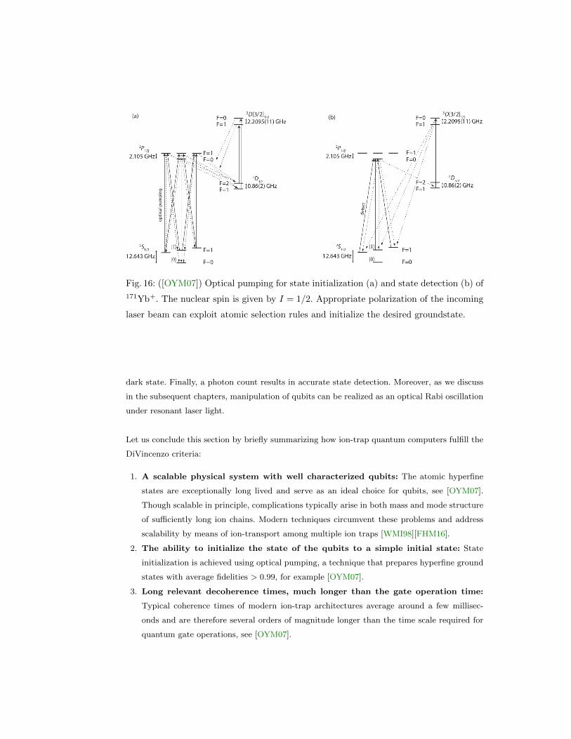
Fig. 16: ([OYM07]) Optical pumping for state initialization (a) and state detection (b) of
171Yb+. The nuclear spin is given by I = 1/2. Appropriate polarization of the incoming
laser beam can exploit atomic selection rules and initialize the desired groundstate.
dark state. Finally, a photon count results in accurate state detection. Moreover, as we discuss
in the subsequent chapters, manipulation of qubits can be realized as an optical Rabi oscillation
under resonant laser light.
Let us conclude this section by briefly summarizing how ion-trap quantum computers fulfill the
DiVincenzo criteria:
1. A scalable physical system with well characterized qubits: The atomic hyperfine
states are exceptionally long lived and serve as an ideal choice for qubits, see [OYM07].
Though scalable in principle, complications typically arise in both mass and mode structure
of sufficiently long ion chains. Modern techniques circumvent these problems and address
scalability by means of ion-transport among multiple ion traps [WMI98][FHM16].
2. The ability to initialize the state of the qubits to a simple initial state: State
initialization is achieved using optical pumping, a technique that prepares hyperfine ground
states with average fidelities > 0.99, for example [OYM07].
3. Long relevant decoherence times, much longer than the gate operation time:
Typical coherence times of modern ion-trap architectures average around a few millisec-
onds and are therefore several orders of magnitude longer than the time scale required for
quantum gate operations, see [OYM07].
4. A universal set of quantum gates: All single-qubit gates can be performed using laser
pulses that drive Rabi oscillations between the two atomic levels. Two-qubit gates are imple-
mented by exploiting the long range Coulomb interaction, such as in the original proposal
by Cirac and Zoller [CZ95]. Quantum information from a single ion can be transferred into
the common motional degree of freedom of the entire ion string using a sideband transition
by focused laser pulses. Such conditional quantum dynamics are sufficient to give rise to
elementary two-qubit gates needed for universal computation. Moreover, sources of error
during larger scale quantum operations can be controlled for by more sophisticated types
of multiparticle entanglement, such as Mølmer-Sørensen interactions [MS99].
5. A qubit-specific measurement capability: Measurements are performed using state
dependent fluorescence in which photon scattering allows for state read-out of individual
qubits.
The Hamiltonian. In this section, we discuss the basic Hamiltonian of a single trapped ion
interacting with near resonant laser light. The two-level approximation is valid in this regime,
as all other atomic levels are energetically far away and highly detuned. Similar to a spin-1/2
system under a time-dependent magnetic field, the two-level atom undergoes an optical Rabi
oscillation under the action of the electromagnetic field.
Let us consider a Hamiltonian of a two-level system interacting with a quantized harmonic
oscillator of vibrational modes through a laser beam, where:
H = Hatom +Hfree +Hint. (166)
Recall from the previous section that the Hamiltonian describing the free motion of a single ion
along the trap axis in an effective harmonic potential can be written as:
Hfree =p2
2M+
1
2Mω2
zz2, (167)
where ωz is the frequency of oscillation around the equilibrium position in the z direction. If the
coupling to the external field is small and the ion inside the vaccum chamber is well isolated
from its surroundings, its motion becomes quantized and we can introduce raising and lowering
operators z =√
~2Mωz
(a + a†) and p = i√
~Mωz2
(a − a†). Consequently, together with the
Hamiltonian corresponding to the internal atomic levels, we can write:
Hatom = ~ωegσz2
(168)
Hfree = ~ωz(a†a+
1
2
). (169)
In the following, we will denote H0 = Hatom +Hfree. The Hamiltonian Hint describes the atom-
light interaction of the ion with the laser. Following Wineland et al. [WBB03], the interaction
between the ion and the electric field of the laser beam is given by:
Hint(t) = −d ·E = −d · E0 εL cos(kz − ωLt+ φ), (170)
where d is the electric dipole operator, E is the (classical) electric field, E0 the field strength, z
is the position operator of the ion for displacement from its equilibrium position, εL is the laser
beam polarization, ωL is the frequency of the laser, k is the laser beam’s k-vector parallel to
z (the axis of the trap) and where φ is the phase of the laser at the mean position of the ion.
In the dipole approximation, d can be further expanded in terms of the internal states of the
atom, since it is proportional to σ+ + σ−, where σ+ = |e〉 〈g| and σ− = |g〉 〈e|. By introducing
the Rabi flop frequency Ω = −E0~ 〈e|d · εL|g〉 and the Lamb-Dicke parameter η = k
√~
2Mωz, we
can express Eq.(170) as:
Hint(t) = ~Ω2
(σ+ + σ−)(ei(η(a+a
†)−ωLt+φ) + e−i(η(a+a†)−ωLt+φ)
). (171)
Taking the width of the ion’s oscillation along the trap axis at low temperatures to be small
compared to the wavelength of the incoming laser beam, we can apply the Lamb-Dicke limit
(η√〈(a+ a†)2〉 1) and further expand the relevant exponential from Eq.(171):
eiη(a+a†) = 1 + iη (a+ a†) + O(η2). (172)
It is now convenient to work in the interaction picture H′int = eiH0t/~Hinte−iH0t/~. Using the
Baker-Campbell-Hausdorff lemma,
eαABe−αA = B + α [A,B] +α2
2![A, [A,B]] +
α3
3![A, [A, [A,B]]] + ..., (173)
we get the following identities:
eiωza†a t[1 + iη (a+ a†)
]e−iωza
†a t = 1 + iη (ae−iωzt + a†eiωzt) (174)
eiωegσzt/2σ+e−iωegσzt/2 = σ+e
iωegt. (175)
By applying a rotating wave approximation and assuming near resonance ∆ = ωL − ωeg ≈ 0,
we ignore all rapidly oscillating terms of the form exp(±i(ωL + ωeg)t) and find:
H′int(t) = ~Ω2σ+ e
−i(∆t−φ)[1 + iη (ae−iωzt + a†eiωzt)
]+ h.c. + O(η2). (176)
A second rotating wave approximation assumes that only one transition at a time is considered,
now gives the Hamiltonian:
H′int(t) =~Ω2
[σ+e
−i(∆t−φ) + σ−ei(∆t−φ) + iη(σ+e
−i(∆t−φ) − σ−e−i(∆t−φ))(ae−iωzt + a†eiωzt)]
(177)
We can now identify three different cases of interest with respect to the detuning of the laser
beam, the so-called carrier and sideband transitions:[HRB08]
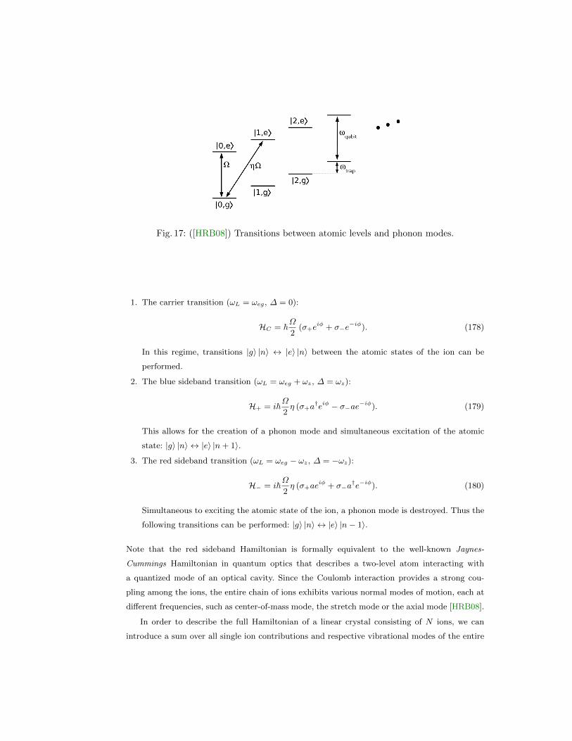
Fig. 17: ([HRB08]) Transitions between atomic levels and phonon modes.
1. The carrier transition (ωL = ωeg, ∆ = 0):
HC = ~Ω2
(σ+eiφ + σ−e
−iφ). (178)
In this regime, transitions |g〉 |n〉 ↔ |e〉 |n〉 between the atomic states of the ion can be
performed.
2. The blue sideband transition (ωL = ωeg + ωz, ∆ = ωz):
H+ = i~Ω2η (σ+a
†eiφ − σ−ae−iφ). (179)
This allows for the creation of a phonon mode and simultaneous excitation of the atomic
state: |g〉 |n〉 ↔ |e〉 |n+ 1〉.
3. The red sideband transition (ωL = ωeg − ωz, ∆ = −ωz):
H− = i~Ω2η (σ+ae
iφ + σ−a†e−iφ). (180)
Simultaneous to exciting the atomic state of the ion, a phonon mode is destroyed. Thus the
following transitions can be performed: |g〉 |n〉 ↔ |e〉 |n− 1〉.
Note that the red sideband Hamiltonian is formally equivalent to the well-known Jaynes-
Cummings Hamiltonian in quantum optics that describes a two-level atom interacting with
a quantized mode of an optical cavity. Since the Coulomb interaction provides a strong cou-
pling among the ions, the entire chain of ions exhibits various normal modes of motion, each at
different frequencies, such as center-of-mass mode, the stretch mode or the axial mode [HRB08].
In order to describe the full Hamiltonian of a linear crystal consisting of N ions, we can
introduce a sum over all single ion contributions and respective vibrational modes of the entire
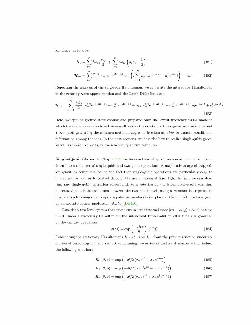
ion chain, as follows:
H0 =
N∑j=1
~ωegσzj2
+
N∑l=1
~ωzl
(a†l al +
1
2
)(181)
H′int =
N∑j=1
~Ωj2
σ+j e−i(∆t−φ) exp
(i
N∑l=1
ηjl [ale−iωzt + a†l e
iωzt]
)+ h.c.. (182)
Repeating the analysis of the single-ion Hamiltonian, we can write the interaction Hamiltonian
in the rotating wave approximation and the Lamb-Dicke limit as:
H′int =
N∑j,l=1
~Ωj2
[σ(j)+ e−i(∆t−φ) + σ
(j)− ei(∆t−φ) + iηjl(σ
(j)+ e−i(∆t−φ) − σ(j)
− ei(∆t−φ))(ale−iωzt + a†l e
iωzt)]
(183)
Here, we applied ground-state cooling and prepared only the lowest frequency COM mode in
which the same phonon is shared among all ions in the crystal. In this regime, we can implement
a two-qubit gate using the common motional degree of freedom as a bus to transfer conditional
information among the ions. In the next sections, we describe how to realize single-qubit gates,
as well as two-qubit gates, in the ion-trap quantum computer.
Single-Qubit Gates. In Chapter 5.4, we discussed how all quantum operations can be broken
down into a sequence of single qubit and two-qubit operations. A major advantage of trapped-
ion quantum computers lies in the fact that single-qubit operations are particularly easy to
implement, as well as to control through the use of resonant laser light. In fact, we can show
that any single-qubit operation corresponds to a rotation on the Bloch sphere and can thus
be realized as a Rabi oscillation between the two qubit levels using a resonant laser pulse. In
practice, such tuning of appropriate pulse parameters takes place at the control interface given
by an acousto-optical modulator (AOM) [DHL05].
Consider a two-level system that starts out in some internal state |ψ〉 = cg |g〉+ce |e〉 at time
t = 0. Under a stationary Hamiltonian, the subsequent time-evolution after time τ is governed
by the unitary dynamics:
|ψ(τ)〉 = exp
(−iHτ
~
)|ψ(0)〉 . (184)
Considering the stationary Hamiltonians HC ,H+ and H− from the previous section under ra-
diation of pulse length τ and respective detuning, we arrive at unitary dynamics which induce
the following rotations:
RC (θ, φ) = exp(−iθ/2 (σ+e
iφ + σ−e−iφ)
)(185)
R+ (θ, φ) = exp(−iθ/2 (σ+a
†eiφ − σ−ae−iφ))
(186)
R− (θ, φ) = exp(−iθ/2 (σ+ae
iφ + σ−a†e−iφ)
), (187)
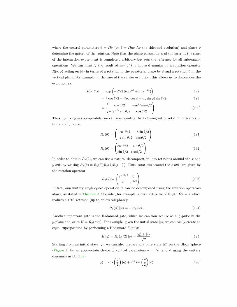
where the control parameters θ = Ωτ (or θ = Ωητ for the sideband evolution) and phase φ
determine the nature of the rotation. Note that the phase parameter φ of the laser at the start
of the interaction experiment is completely arbitrary but sets the reference for all subsequent
operations. We can identify the result of any of the above dynamics by a rotation operator
R(θ, φ) acting on |ψ〉 in terms of a rotation in the equatorial plane by φ and a rotation θ in the
vertical plane. For example, in the case of the carrier evolution, this allows us to decompose the
evolution as:
RC (θ, φ) = exp(−iθ/2 (σ+e
iφ + σ−e−iφ)
)(188)
= 1 cos θ/2− i(σx cosφ− σy sinφ) sin θ/2 (189)
=
cos θ/2 −ieiφ sin θ/2
−ie−iφ sin θ/2 cos θ/2
(190)
Thus, by fixing φ appropriately, we can now identify the following set of rotation operators in
the x and y plane:
Rx(θ) =
cos θ/2 −i sin θ/2
−i sin θ/2 cos θ/2
(191)
Ry(θ) =
cos θ/2 − sin θ/2
sin θ/2 cos θ/2
(192)
In order to obtain Rz(θ), we can use a natural decomposition into rotations around the x and
y axis by writing Rz(θ) = Ry(π2
)Rx(θ)Ry(−π2
). Thus, rotations around the z axis are given by
the rotation operator:
Rz(θ) =
e−iθ/2 0
0 eiθ/2
(193)
In fact, any unitary single-qubit operation U can be decomposed using the rotation operators
above, as stated in Theorem 3. Consider, for example, a resonant pulse of length Ωτ = π which
realizes a 180 rotation (up to an overall phase):
Rx(π) |ψ〉 = −iσx |ψ〉 . (194)
Another important gate is the Hadamard gate, which we can now realize as a π2
-pulse in the
y-plane and write H = Ry(π/2). For example, given the initial state |g〉, we can easily create an
equal superposition by performing a Hadamard π2
-pulse:
H |g〉 = Ry(π/2) |g〉 =|g〉+ |e〉√
2. (195)
Starting from an initial state |g〉, we can also prepare any pure state |ψ〉 on the Bloch sphere
(Figure 1) by an appropriate choice of control parameters θ = Ωτ and φ using the unitary
dynamics in Eq.(188):
|ψ〉 = cos
(θ
2
)|g〉+ eiφ sin
(θ
2
)|e〉 . (196)
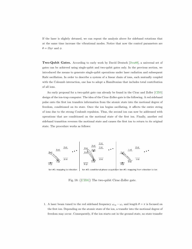
If the laser is slightly detuned, we can repeat the analysis above for sideband rotations that
at the same time increase the vibrational modes. Notice that now the control parameters are
θ = Ωητ and φ.
Two-Qubit Gates. According to early work by David Deutsch [Deu89], a universal set of
gates can be achieved using single-qubit and two-qubit gates only. In the previous section, we
introduced the means to generate single-qubit operations under laser radiation and subsequent
Rabi oscillation. In order to describe a system of a linear chain of ions, each mutually coupled
with the Coloumb interaction, one has to adopt a Hamiltonian that includes total contribution
of all ions.
An early proposal for a two-qubit gate can already be found in the Cirac and Zoller [CZ95]
design of the ion-trap computer. The idea of the Cirac-Zoller-gate is the following. A red sideband
pulse onto the first ion transfers information from the atomic state into the motional degree of
freedom, conditioned on its state. Once the ion begins oscillating, it affects the entire string
of ions due to the strong Coulomb repulsion. Thus, the second ion can now be addressed with
operations that are conditioned on the motional state of the first ion. Finally, another red
sideband transition reverses the motional state and causes the first ion to return to its original
state. The procedure works as follows:
Fig. 18: ([CZ01]) The two-qubit Cirac-Zoller gate.
1. A laser beam tuned to the red sideband frequency ωeg − ωz and length θ = π is focused on
the first ion. Depending on the atomic state of the ion, a transfer into the motional degree of
freedom may occur. Consequently, if the ion starts out in the ground state, no state transfer
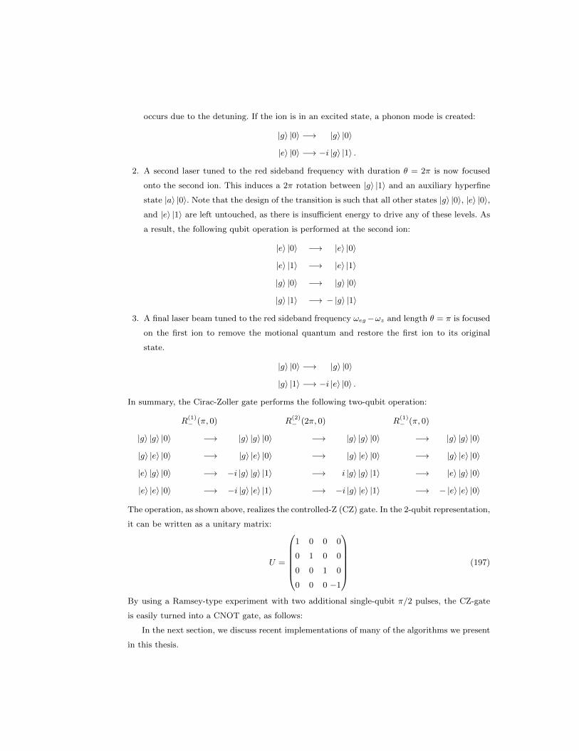
occurs due to the detuning. If the ion is in an excited state, a phonon mode is created:
|g〉 |0〉 −→ |g〉 |0〉
|e〉 |0〉 −→ −i |g〉 |1〉 .
2. A second laser tuned to the red sideband frequency with duration θ = 2π is now focused
onto the second ion. This induces a 2π rotation between |g〉 |1〉 and an auxiliary hyperfine
state |a〉 |0〉. Note that the design of the transition is such that all other states |g〉 |0〉, |e〉 |0〉,
and |e〉 |1〉 are left untouched, as there is insufficient energy to drive any of these levels. As
a result, the following qubit operation is performed at the second ion:
|e〉 |0〉 −→ |e〉 |0〉
|e〉 |1〉 −→ |e〉 |1〉
|g〉 |0〉 −→ |g〉 |0〉
|g〉 |1〉 −→ − |g〉 |1〉
3. A final laser beam tuned to the red sideband frequency ωeg−ωz and length θ = π is focused
on the first ion to remove the motional quantum and restore the first ion to its original
state.
|g〉 |0〉 −→ |g〉 |0〉
|g〉 |1〉 −→ −i |e〉 |0〉 .
In summary, the Cirac-Zoller gate performs the following two-qubit operation:
R(1)− (π, 0) R
(2)− (2π, 0) R
(1)− (π, 0)
|g〉 |g〉 |0〉 −→ |g〉 |g〉 |0〉 −→ |g〉 |g〉 |0〉 −→ |g〉 |g〉 |0〉
|g〉 |e〉 |0〉 −→ |g〉 |e〉 |0〉 −→ |g〉 |e〉 |0〉 −→ |g〉 |e〉 |0〉
|e〉 |g〉 |0〉 −→ −i |g〉 |g〉 |1〉 −→ i |g〉 |g〉 |1〉 −→ |e〉 |g〉 |0〉
|e〉 |e〉 |0〉 −→ −i |g〉 |e〉 |1〉 −→ −i |g〉 |e〉 |1〉 −→ − |e〉 |e〉 |0〉
The operation, as shown above, realizes the controlled-Z (CZ) gate. In the 2-qubit representation,
it can be written as a unitary matrix:
U =
1 0 0 0
0 1 0 0
0 0 1 0
0 0 0 −1
(197)
By using a Ramsey-type experiment with two additional single-qubit π/2 pulses, the CZ-gate
is easily turned into a CNOT gate, as follows:
In the next section, we discuss recent implementations of many of the algorithms we present
in this thesis.
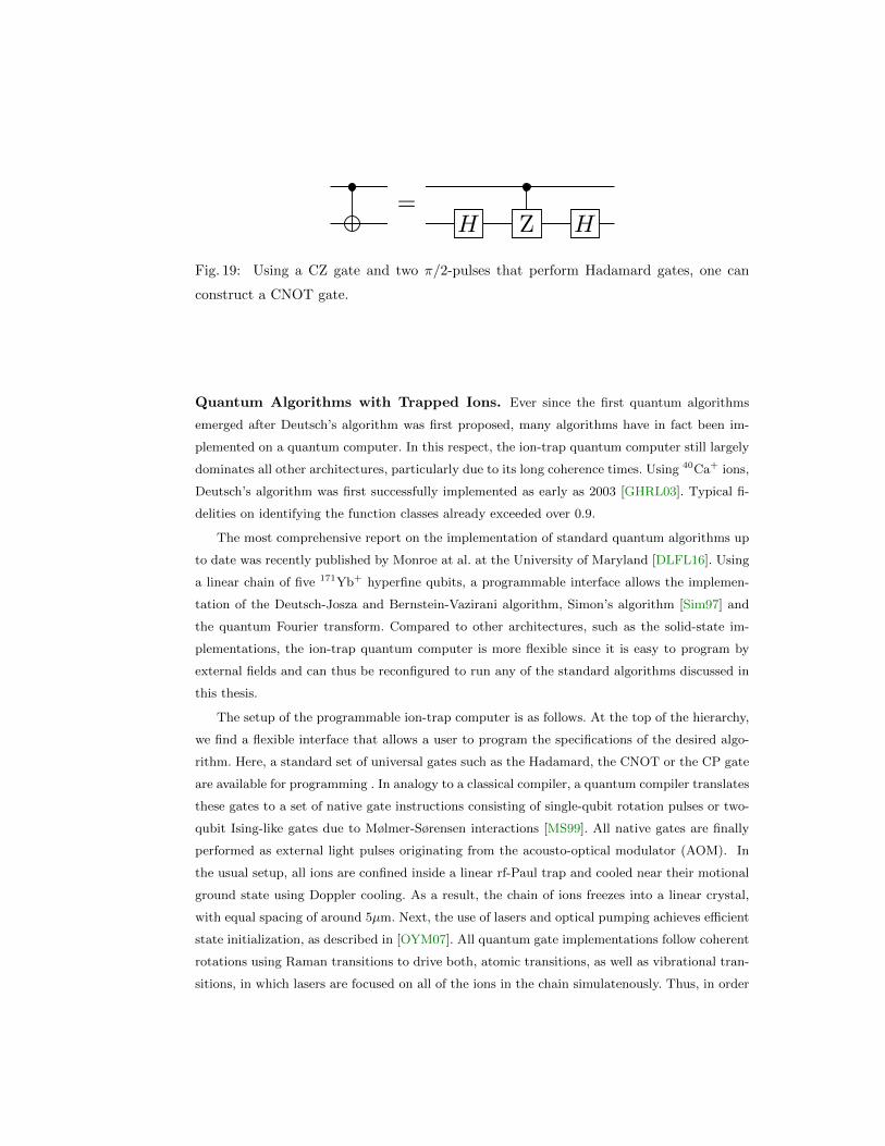
=H Z H
Fig. 19: Using a CZ gate and two π/2-pulses that perform Hadamard gates, one can
construct a CNOT gate.
Quantum Algorithms with Trapped Ions. Ever since the first quantum algorithms
emerged after Deutsch’s algorithm was first proposed, many algorithms have in fact been im-
plemented on a quantum computer. In this respect, the ion-trap quantum computer still largely
dominates all other architectures, particularly due to its long coherence times. Using 40Ca+ ions,
Deutsch’s algorithm was first successfully implemented as early as 2003 [GHRL03]. Typical fi-
delities on identifying the function classes already exceeded over 0.9.
The most comprehensive report on the implementation of standard quantum algorithms up
to date was recently published by Monroe at al. at the University of Maryland [DLFL16]. Using
a linear chain of five 171Yb+ hyperfine qubits, a programmable interface allows the implemen-
tation of the Deutsch-Josza and Bernstein-Vazirani algorithm, Simon’s algorithm [Sim97] and
the quantum Fourier transform. Compared to other architectures, such as the solid-state im-
plementations, the ion-trap quantum computer is more flexible since it is easy to program by
external fields and can thus be reconfigured to run any of the standard algorithms discussed in
this thesis.
The setup of the programmable ion-trap computer is as follows. At the top of the hierarchy,
we find a flexible interface that allows a user to program the specifications of the desired algo-
rithm. Here, a standard set of universal gates such as the Hadamard, the CNOT or the CP gate
are available for programming . In analogy to a classical compiler, a quantum compiler translates
these gates to a set of native gate instructions consisting of single-qubit rotation pulses or two-
qubit Ising-like gates due to Mølmer-Sørensen interactions [MS99]. All native gates are finally
performed as external light pulses originating from the acousto-optical modulator (AOM). In
the usual setup, all ions are confined inside a linear rf-Paul trap and cooled near their motional
ground state using Doppler cooling. As a result, the chain of ions freezes into a linear crystal,
with equal spacing of around 5µm. Next, the use of lasers and optical pumping achieves efficient
state initialization, as described in [OYM07]. All quantum gate implementations follow coherent
rotations using Raman transitions to drive both, atomic transitions, as well as vibrational tran-
sitions, in which lasers are focused on all of the ions in the chain simulatenously. Thus, in order
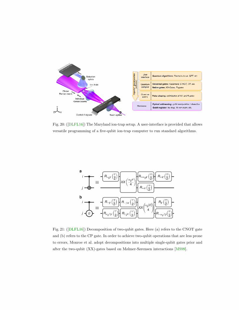
Fig. 20: ([DLFL16]) The Maryland ion-trap setup. A user-interface is provided that allows
versatile programming of a five-qubit ion-trap computer to run standard algorithms.
Fig. 21: ([DLFL16]) Decomposition of two-qubit gates. Here (a) refers to the CNOT gate
and (b) refers to the CP gate. In order to achieve two-qubit operations that are less prone
to errors, Monroe et al. adopt decompositions into multiple single-qubit gates prior and
after the two-qubit (XX)-gates based on Mølmer-Sørensen interactions [MS99].
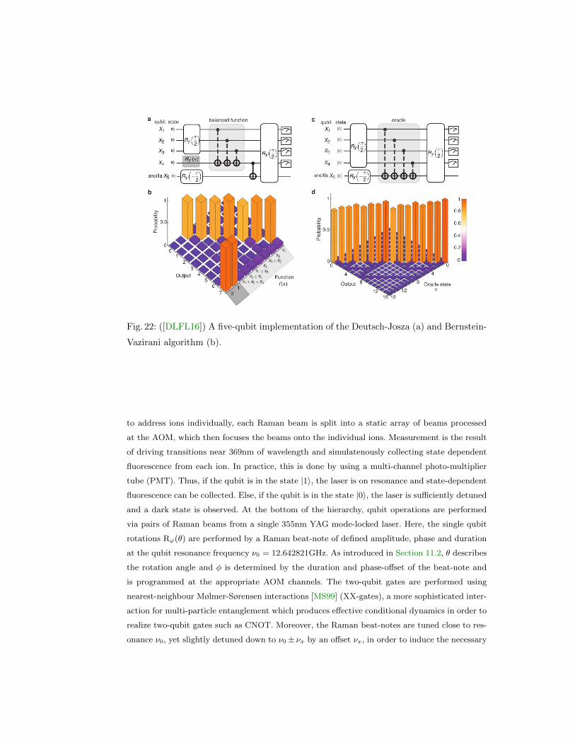
Fig. 22: ([DLFL16]) A five-qubit implementation of the Deutsch-Josza (a) and Bernstein-
Vazirani algorithm (b).
to address ions individually, each Raman beam is split into a static array of beams processed
at the AOM, which then focuses the beams onto the individual ions. Measurement is the result
of driving transitions near 369nm of wavelength and simulatenously collecting state dependent
fluorescence from each ion. In practice, this is done by using a multi-channel photo-multiplier
tube (PMT). Thus, if the qubit is in the state |1〉, the laser is on resonance and state-dependent
fluorescence can be collected. Else, if the qubit is in the state |0〉, the laser is sufficiently detuned
and a dark state is observed. At the bottom of the hierarchy, qubit operations are performed
via pairs of Raman beams from a single 355nm YAG mode-locked laser. Here, the single qubit
rotations Rϕ(θ) are performed by a Raman beat-note of defined amplitude, phase and duration
at the qubit resonance frequency ν0 = 12.642821GHz. As introduced in Section 11.2, θ describes
the rotation angle and φ is determined by the duration and phase-offset of the beat-note and
is programmed at the appropriate AOM channels. The two-qubit gates are performed using
nearest-neighbour Mølmer-Sørensen interactions [MS99] (XX-gates), a more sophisticated inter-
action for multi-particle entanglement which produces effective conditional dynamics in order to
realize two-qubit gates such as CNOT. Moreover, the Raman beat-notes are tuned close to res-
onance ν0, yet slightly detuned down to ν0± νx by an offset νx, in order to induce the necessary
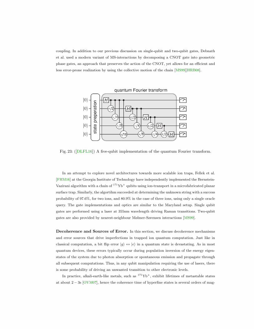
coupling. In addition to our previous discussion on single-qubit and two-qubit gates, Debnath
et al. used a modern variant of MS-interactions by decomposing a CNOT gate into geometric
phase gates, an approach that preserves the action of the CNOT, yet allows for an efficient and
less error-prone realization by using the collective motion of the chain [MS99][HRB08].
Fig. 23: ([DLFL16]) A five-qubit implementation of the quantum Fourier transform.
In an attempt to explore novel architectures towards more scalable ion traps, Fellek et al.
[FHM16] at the Georgia Institute of Technology have independently implemented the Bernstein-
Vazirani algorithm with a chain of 171Yb+ qubits using ion-transport in a microfabricated planar
surface trap. Similarly, the algortihm succeeded at determining the unknown string with a success
probability of 97.6%, for two ions, and 80.9% in the case of three ions, using only a single oracle
query. The gate implementations and optics are similar to the Maryland setup. Single qubit
gates are performed using a laser at 355nm wavelength driving Raman transitions. Two-qubit
gates are also provided by nearest-neighbour Mølmer-Sørensen interactions [MS99].
Decoherence and Sources of Error. In this section, we discuss decoherence mechanisms
and error sources that drive imperfections in trapped ion quantum computation. Just like in
classical computation, a bit flip error |g〉 ↔ |e〉 in a quantum state is devastating. As in most
quantum devices, these errors typically occur during population inversion of the energy eigen-
states of the system due to photon absorption or spontaneous emission and propagate through
all subsequent computations. Thus, in any qubit manipulation requiring the use of lasers, there
is some probability of driving an unwanted transition to other electronic levels.
In practice, alkali-earth-like metals, such as 171Yb+, exhibit lifetimes of metastable states
at about 2− 3s [OYM07], hence the coherence time of hyperfine states is several orders of mag-
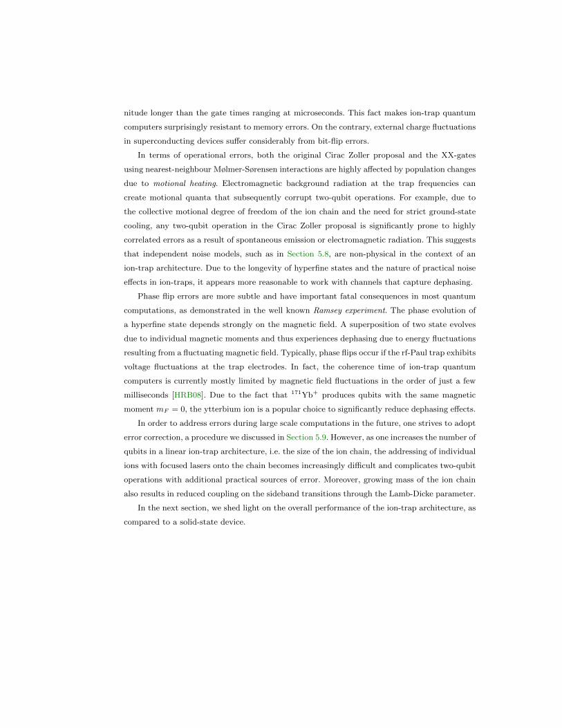
nitude longer than the gate times ranging at microseconds. This fact makes ion-trap quantum
computers surprisingly resistant to memory errors. On the contrary, external charge fluctuations
in superconducting devices suffer considerably from bit-flip errors.
In terms of operational errors, both the original Cirac Zoller proposal and the XX-gates
using nearest-neighbour Mølmer-Sørensen interactions are highly affected by population changes
due to motional heating. Electromagnetic background radiation at the trap frequencies can
create motional quanta that subsequently corrupt two-qubit operations. For example, due to
the collective motional degree of freedom of the ion chain and the need for strict ground-state
cooling, any two-qubit operation in the Cirac Zoller proposal is significantly prone to highly
correlated errors as a result of spontaneous emission or electromagnetic radiation. This suggests
that independent noise models, such as in Section 5.8, are non-physical in the context of an
ion-trap architecture. Due to the longevity of hyperfine states and the nature of practical noise
effects in ion-traps, it appears more reasonable to work with channels that capture dephasing.
Phase flip errors are more subtle and have important fatal consequences in most quantum
computations, as demonstrated in the well known Ramsey experiment. The phase evolution of
a hyperfine state depends strongly on the magnetic field. A superposition of two state evolves
due to individual magnetic moments and thus experiences dephasing due to energy fluctuations
resulting from a fluctuating magnetic field. Typically, phase flips occur if the rf-Paul trap exhibits
voltage fluctuations at the trap electrodes. In fact, the coherence time of ion-trap quantum
computers is currently mostly limited by magnetic field fluctuations in the order of just a few
milliseconds [HRB08]. Due to the fact that 171Yb+ produces qubits with the same magnetic
moment mF = 0, the ytterbium ion is a popular choice to significantly reduce dephasing effects.
In order to address errors during large scale computations in the future, one strives to adopt
error correction, a procedure we discussed in Section 5.9. However, as one increases the number of
qubits in a linear ion-trap architecture, i.e. the size of the ion chain, the addressing of individual
ions with focused lasers onto the chain becomes increasingly difficult and complicates two-qubit
operations with additional practical sources of error. Moreover, growing mass of the ion chain
also results in reduced coupling on the sideband transitions through the Lamb-Dicke parameter.
In the next section, we shed light on the overall performance of the ion-trap architecture, as
compared to a solid-state device.
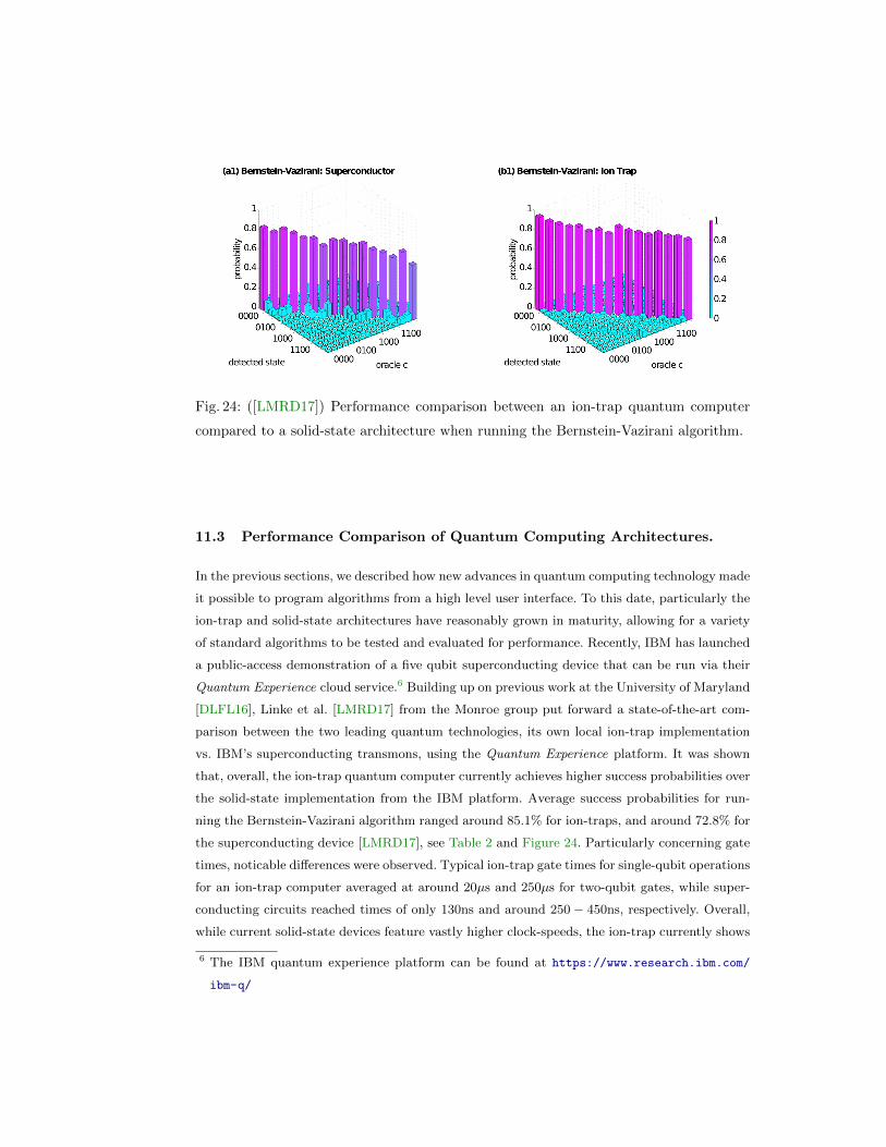
Fig. 24: ([LMRD17]) Performance comparison between an ion-trap quantum computer
compared to a solid-state architecture when running the Bernstein-Vazirani algorithm.
11.3 Performance Comparison of Quantum Computing Architectures.
In the previous sections, we described how new advances in quantum computing technology made
it possible to program algorithms from a high level user interface. To this date, particularly the
ion-trap and solid-state architectures have reasonably grown in maturity, allowing for a variety
of standard algorithms to be tested and evaluated for performance. Recently, IBM has launched
a public-access demonstration of a five qubit superconducting device that can be run via their
Quantum Experience cloud service.6 Building up on previous work at the University of Maryland
[DLFL16], Linke et al. [LMRD17] from the Monroe group put forward a state-of-the-art com-
parison between the two leading quantum technologies, its own local ion-trap implementation
vs. IBM’s superconducting transmons, using the Quantum Experience platform. It was shown
that, overall, the ion-trap quantum computer currently achieves higher success probabilities over
the solid-state implementation from the IBM platform. Average success probabilities for run-
ning the Bernstein-Vazirani algorithm ranged around 85.1% for ion-traps, and around 72.8% for
the superconducting device [LMRD17], see Table 2 and Figure 24. Particularly concerning gate
times, noticable differences were observed. Typical ion-trap gate times for single-qubit operations
for an ion-trap computer averaged at around 20µs and 250µs for two-qubit gates, while super-
conducting circuits reached times of only 130ns and around 250 − 450ns, respectively. Overall,
while current solid-state devices feature vastly higher clock-speeds, the ion-trap currently shows
6 The IBM quantum experience platform can be found at https://www.research.ibm.com/
ibm-q/
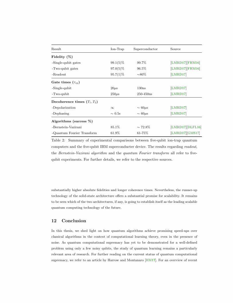
Result Ion-Trap Superconductor Source
Fidelity (%)
-Single-qubit gates 99.1(5)% 99.7% [LMRD17][FHM16]
-Two-qubit gates 97.0(5)% 96.5% [LMRD17][FHM16]
-Readout 95.7(1)% ∼80% [LMRD17]
Gate times (τop)
-Single-qubit 20µs 130ns [LMRD17]
-Two-qubit 250µs 250-450ns [LMRD17]
Decoherence times (T1, T2)
-Depolarization ∞ ∼ 60µs [LMRD17]
-Dephasing ∼ 0.5s ∼ 60µs [LMRD17]
Algorithms (success %)
-Bernstein-Vazirani 85.1% ∼ 72.8% [LMRD17][DLFL16]
-Quantum Fourier Transform 61.9% 61-75% [LMRD17][GMS17]
Table 2: Summary of experimental comparisons between five-qubit ion-trap quantum
computers and the five-qubit IBM superconducter device. The results regarding readout,
the Bernstein-Vazirani algorithm and the quantum Fourier transform all refer to five-
qubit experiments. For further details, we refer to the respective sources.
substantially higher absolute fidelities and longer coherence times. Nevertheless, the runner-up
technology of the solid-state architecture offers a substantial promise for scalability. It remains
to be seen which of the two architectures, if any, is going to establish itself as the leading scalable
quantum computing technology of the future.
12 Conclusion
In this thesis, we shed light on how quantum algorithms achieve promising speed-ups over
classical algorithms in the context of computational learning theory, even in the presence of
noise. As quantum computational supremacy has yet to be demonstrated for a well-defined
problem using only a few noisy qubits, the study of quantum learning remains a particularly
relevant area of research. For further reading on the current status of quantum computational
supremacy, we refer to an article by Harrow and Montanaro [HM17]. For an overview of recent
progress in quantum learning theory, we refer to the survey by Arunachalam and de Wolf
[AdW17].
By investigating the limitations of quantum algorithms through the use of relabeling, we
proposed suitable constructions for new notions of security under non-adaptive quantum chosen-
ciphertext attacks. The pursuit of useful quantum-secure classical encryption schemes remains
one of the key challenges in post-quantum cryptography. Therefore, further research is now
needed to investigate whether classical communication is ultimately feasibile in a quantum
world. Finally, for further reading on the current status of post-quantum cryptography, we refer
to a recent article by Bernstein and Lange [BL17].
13 Open Problems
Due to the fact that LWE is easy once algorithms receive quantum superposition access to noisy
samples on the secret string, it is tempting to explore circumstances in cryptography under
which such access is granted. While it is reasonable to assume that providing such quantum
access is ill-advised for public-key cryptography, it remains an open problem whether there are
other realistic scenarios. One possible direction to investigate is program obfuscation, a recent
breakthrough in cryptography which concerns the process of obscuring software or code in order
to preserve functionality, yet hide sensitive information on the program itself with at most
polynomial slowdown. An attacker in possession of a quantum computer could, in principle,
implement the obfuscated circuit and then query it in superposition. Since indistinguishability
obfuscation allows us to turn symmetric-key encryption schemes into public-key encryption
schemes [SW14], this could potentially open up a door to providing quantum access to LWE
samples in the context of the LWE-SKES.
Many of the classical notions of security are still widely unexplored in a quantum world, mak-
ing both quantum cryptography and classical quantum-safe cryptography a highly relevant field
of research. In 2016, Gagliardoni, Hulsing and Schaffner [GHS16] provided security standards
of quantum indistuingishability under quantum chosen-plaintext-attacks and proposed secure
quantum encryption schemes for which such security notions can be achieved. Further research
is now needed to investigate secure constructions under a quantum chosen-ciphertext attack,
in particular regarding a quantum indistinguishability notion of QIND-QCCA1. This indistin-
guishability setting naturally generalizes the QCCA1 learning phase we considered in this thesis
to a now fully quantum challenge phase in which the challenge ciphertext is also a quantum
state. Thus, in the QIND-QCCA1 indistinguishability game, both the learning phase and the
challenge phase concern fully quantum communication. While many classical constructions for
CCA2 security already exist, it also remains an open problem to define a fully quantum notion
of indistinguishability for QCCA2 that allows for secure quantum encryption schemes.
Acknowledgments
I want to thank my supervisor Gorjan Alagic for his support and mentorship, and for inspiring
me to pursue a thesis in cryptography. I also want to thank Thomas Gasenzer for making this
thesis collaboration possible. Finally, I want to thank everyone who offered additional support,
contributed with comments or engaged in useful discussions, especially everyone at QMATH:
Matthias Christandl, Florian Speelman, Chris Perry, Roberto Ferrara and Christian Majenz, as
well as Benjamin Freist at Heidelberg University.
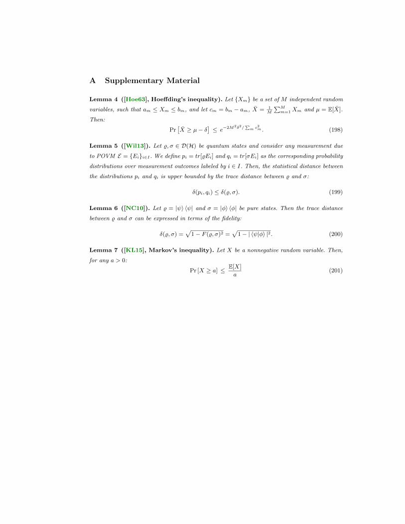
A Supplementary Material
Lemma 4 ([Hoe63], Hoeffding’s inequality). Let Xm be a set of M independent random
variables, such that am ≤ Xm ≤ bm, and let cm = bm − am, X = 1M
∑Mm=1Xm and µ = E[X].
Then:
Pr[X ≥ µ− δ
]≤ e−2M2δ2/
∑m c2m . (198)
Lemma 5 ([Wil13]). Let %,σ ∈ D(H) be quantum states and consider any measurement due
to POVM E = Eii∈I . We define pi = tr[%Ei] and qi = tr[σEi] as the corresponding probability
distributions over measurement outcomes labeled by i ∈ I. Then, the statistical distance between
the distributions pi and qi is upper bounded by the trace distance between % and σ:
δ(pi, qi) ≤ δ(%, σ). (199)
Lemma 6 ([NC10]). Let % = |ψ〉 〈ψ| and σ = |φ〉 〈φ| be pure states. Then the trace distance
between % and σ can be expressed in terms of the fidelity:
δ(%, σ) =√
1− F (%, σ)2 =√
1− | 〈ψ|φ〉 |2. (200)
Lemma 7 ([KL15], Markov’s inequality). Let X be a nonnegative random variable. Then,
for any a > 0:
Pr [X ≥ a] ≤ E[X]
a(201)
Bibliography
[AB08] Aharonov, D., and M. Ben-Or, Fault-tolerant quantum computation with constant error
rate, SIAM Journal on Computing 38(4), pp. 1207-1282, 2008.
[AdW17] Arunachalam, S., de Wolf, R., A survey of quantum learning theory, CoRR,
abs/1701.06806, 2017.
[ASR18] Alagic, G., Song, F., Russel, A., Private Communication, 2018.
[BB84] Bennett, C., Brassard, G., Quantum cryptography: Public key distribution and coin toss-
ing, In Proceedings of the International Conference on Computers, Systems, and Signal
Processing, pages 175-179, 1984.
[BKW94] Blum, A., Furst, M.L., Kearns, M.J., Lipton, R.J., Cryptographic Primitives Based on
Hard Learning Problems, Stinson, D.R. (ed.) CRYPTO 1993. LNCS, vol. 773, pp. 278-291.
Springer, Heidelberg, 1994.
[BKW03] Blum, A., Kalai, A., and Wasserman, H., Noise-tolerant learning, the parity problem,
and the statistical query model, Journal of the ACM, 50(4):506-519, 2003.
[BL17] Bernstein, D., J., Lange, T., Post-quantum cryptography, Nature 549, 188-194,
doi:10.1038/nature23461, 2017.
[BV93] Bernstein, E., Vazirani, U., Quantum Complexity Theory, Proc. 25th ACM Symposium
on Theory of Computation, pp. 11-20, 1993.
[BZ13] Boneh, D., Zhandry, M., Secure Signatures and Chosen Ciphertext Security in a Quan-
tum Computing World, Proceedings of CRYPTO, 2013.
[CD10] Childs, A., van Dam, W., Quantum algorithms for algebraic problems, Reviews of Mod-
ern Physics 82, 1-52, 2010.
[CSS14] Cross, A. W., Smith, G., Smolin, J. A., Quantum learning robust against noise, Physical
Review A, 92(1):012327, 2015.
[CZ95] Cirac, J. I., Zoller, P., Quantum computations with cold trapped ions, Phys. Rev. Lett.
74 (20), 4091-4094, 1995.
[CZ97] Cirac, I., Zoller, P., Kimble, J., Mabuchi, H., Quantum state transfer and entanglement
distribution among distant nodes in a quantum network, Phys. Rev. Lett. 78, 3221, 1997.
[CZ01] Cirac, J. I., Duan, L. M., Zoller, P., Quantum optical implementation of quantum infor-
mation processing, Lecture notes, ”Experimental Quantum Computation and Information”
Proceedings of the International School of Physics ”Enrico Fermi” (2001), Course CXLVIII,
p. 263, arXiv:quant-ph/0405030v1
[Deu85] Deutsch, D., Quantum theory, the Church-Turing principle and the universal quantum
computer, Proceedings of the Royal Society of London A400, pp. 97-117, 1985.
[Deu89] Deutsch, D., Quantum Computational Networks, Proceedings of the Royal Society of
London A425:73, 1989.
[DHL05] Donley, E. A., Heavner, T. P., Levi, F., Tataw, M. O., Jefferts, S. R., Double-pass
acousto-optic modulator system, Rev. Sci. Inst. 76, 063112, 2005.
[DiV00] DiVincenzo, D., The Physical Implementation of Quantum Computation, Fortschritte
der Physik, Volume 48, Issue 9-11 September, pages 771-783, 2000.
[DJ92] Deutsch, D., Josza, R., Rapid solution of problems by quantum computation, Proc. R.
Soc. Lond. A 1992 439 553-558; DOI: 10.1098/rspa.1992.0167, 1992.
[DLFL16] Debnath, S., Linke, N. M., Figatt, C., Landsman, K. A., Wright, K., Monroe, C.,
Demonstration of a small programmable quantum computer with atomic qubits, Nature 536,
63-66, (04 August 2016) doi:10.1038/nature18648, 2016.
[Fey82] Feynman, R., Simulating physics with computers, Int. J. Theoret. Phys. 21, 467, 1982.
[FHM16] Fallek, S. D., Herold, C. D., McMahon, B. J., Maller, K. M., Brown, K. R., Amini, J.
M., 1,5 Transport implementation of the Bernstein-Vazirani algorithm with ion qubits, New
J. Phys. 18 (2016), doi:10.1088/1367-2630/18/8/083030, 2016.
[GGM86] Goldreich, O., Goldwasser, S., Micali, S., How to construct random functions, Journal
of the ACM , 33(4):792-807, 1986.
[GHRL03] Gulde, S., Haffner, H., Riebe, M., Lancaster, G., Becher, C., Eschner, J., Schmidt-
Kaler, F., Chuang, I. L., Blatt, R., Quantum information processing with trapped Ca+ ions,
Proc. R. Soc. Lond. A 361, 1363-1374, 2003.
[GHS16] Gagliardoni, T., Hulsing, A., Schaffner, C., Semantic security and indistinguishability
in the quantum world, in Advances in Cryptology - CRYPTO 2016 - 36th Annual Interna-
tional Cryptology Conference, Santa Barbara, CA, USA, August 14-18, 2016, Proceedings,
Part III, pages 60-89, 2016.
[GK17] Grilo, A., Kerenidis, I., Learning with Errors is easy with quantum samples, as appeared
in QCRYPT’17, Cambridge, UK, 2017.
[GMS17] Garcia-Martin, D,, Sierra German, Five Experimental Tests on the 5-qubit IBM Quan-
tum Computer, arXiv:1712.05642, 2017.
[Gol04] Goldreich, O., Foundations of Cryptography: Volume 2, Cambridge University Press,
New York, NY, USA, 2004.
[Gro96] Grover, L., A fast quantum mechanical algorithm for database search, In STOC, pages
212-219, ACM, 22-24, 1996.
[HH00] Hales, L., Hallgren, S., An improved quantum Fourier transform algorithm and applica-
tions, Proceedings of the 41st IEEE Symposium, pp. 515- 525, 2000.
[HM17] Harrow, A., W., Montanaro, A., Quantum computational supremacy, Nature 549, 203-
209, doi:10.1038/nature23458, 2017.
[Hoe63] Hoeffding, W., Probability inequalities for sums of bounded random variables, Journal
of the American Statistical Association. 58 (301): 13-30. 1963.
[HRB08] H. Haffner, C.F. Roos, R. Blatt, Quantum computing with trapped ions, Phys. Rep.
469, 155-203, 2008.
[Kit95] Kitaev, A. Y., Quantum measurements and the Abelian stabilizer problem, arXive e-
print quant-ph/9511026, 1995.
[Kit97] Kitaev, A. Y., Quantum operations: Algorithms and error correction, RMS: Russian
Mathematical Surveys, 52(6):1191-1249, 1997.
[KL15] Katz, J., Lindell, Y., Introduction to Modern Cryptography, CRC Press, 2nd Edition,
2015.
[KLLP16] Kaplan, M., Leurent, G., Leverrier, A., Naya-Plasencia, M., Breaking Symmet-
ric Cryptosystems using Quantum Period Finding, CRYPTO, Springer, pages 207-233,
doi=10.1007/978-3-662-53008-5-8, 2016.
[KY00] Katz, J., Yung, M., Characterization of Security Notions for Probabilistic Private-Key
Encryption, STOC, 2000.
[LOJC05] Langer, C., Ozeri, R., Jost, J. D., Chiaverini, J., Demarco, B., Ben-Kish, A.,
Blakestad, R. B., Britton, J., Hume, D. B., Itano, W. M., Leibfried, D., Reichle, R., Rosen-
band, T., Schaetz, T., Schmidt, P. O., Wineland, D. J., Long-lived qubit memory using
atomic ions, Phys. Rev. Lett. 95, 060502, 2005.
[LMRD17] Linke, N. M., Maslov, D., Roetteler, M., Debnath, S., Figatt, C., Landsman, K.
A., Wright, K., Monroe, C., Experimental Comparison of Two Quantum Computing Archi-
tectures, doi: 10.1073/pnas.1618020114, PNAS March 28, 2017, vol. 114 no. 13 3305-3310,
2017.
[MMKW99] Monroe, C., Meekhof, D. M., King, B. E., Itano, W. M., Wineland, D. J., Demon-
stration of a fundamental quantum logic gate, Phys. Rev. Lett. 75 (25), 4714-4717, 1995.
[Mon13] Monroe, C., Quantum Simulations with Trapped Atomic Ions, Slides from the Varenna
Summer School on Ion Traps and Quantum Simulation, 2013. http://iontrap.umd.edu/
wp-content/uploads/2014/01/Lecture1_QSIM.pptx, (04.11.2017).
[MS99] Mølmer K., Sørensen A., Multiparticle entanglement of hot trapped ions, Phys. Rev.
Lett. 82:1835-1838, 1999.
[NC10] Nielsen, M. A., Chuang, I. L., Quantum Computation and Quantum Information, Cam-
bridge Univ. Press, Cambridge, 9th ed., 2010.
[OYM07] S. Olmschenk, K. C. Younge, D. L. Moehring, D. Matsukevich, P. Maunz, C. Mon-
roe, Manipulation and Detection of a Trapped Yb+ Ion Hyperfine Qubit, Phys. Rev. A 76,
052314, Published 19 November, 2007.
[Pau90] Paul, W., Electromagnetic traps for charged and neutral particles, Rev. Mod. Phys., vol.
62, pages 531-540, 1990.
[POF58] Paul, W., Osberghaus, O., and Fischer, E., Ein Ionenkafig, Forschungsberichte des
Wirtschafts- und Verkehrsministeriums Nordrhein-Westfalen 415, Westfalischer Verlag, 4,
15, 1958.
[Pre98] Preskill, J., Reliable quantum computers, Proceedings of the Royal Society A 454, pp.
385-410, eprint quant-ph/9705031, 1998.
[Reg05] Regev, O., On lattices, learning with errors, random linear codes, and cryptography,
Journal of the ACM, 56(6):34, 2009. Preliminary version in STOC’05.
[Reg09] Regev, O., The Learning with Errors problem, Invited survey in CCC 2010, www.cims.
nyu.edu/~regev/papers/lwesurvey.pdf, 2009.
[RS62] Rosser, J. Barkley; Schoenfeld, Lowell, Approximate formulas for some functions of
prime numbers, Illinois J. Math. 6 (1): 64-94, 1962.
[Sha48] Shannon, C., A Mathematical Theory of Communication, Bell System Technical Jour-
nal. 27 (3): 379-423. doi:10.1002/j.1538-7305.1948.tb01338.x, 1948.
[Sho94] Shor, P. W., Algorithms for quantum computation: discrete logarithms and factoring,
Proceedings of the 35th Annual Symposium on Foundations of Computer Science, Santa
Fe, NM, Nov. 20-22, IEEE Computer Society Press, pp. 124-134, 1994.
[Sho95] Shor, P. W., Scheme for reducing decoherence in quantum computer memory, Phys.
Rev. A 52, R2493(R), 1995.
[Sim97] Simon, D.R., On the power of quantum computation, SIAM journal on computing 26(5),
1474-1483, 1997.
[SW14] Sahai, A., Waters, B., How to use indistinguishability obfuscation: Deniable encryption,
and more., STOC, 2014.
[WBB03] D. J. Wineland, M. Barrett, J. Britton, J. Chiaverini, B. DeMarco, W. M. Itano,
B. Jelenkovic, C. Langer, D. Leibfried, V. Meyer, T. Rosenband, T. Schatz, Quantum
information processing with trapped ions, Phil. Trans. Royal Soc. London A, vol. 361, no.
1808, pages 1349-1361, 2003.
[WI79] Wineland, D. J. and Itano, W. M., Laser cooling of atoms, Phys. Rev. A, 20, 1521-1540,
1979.
[WMI98] D.J. Wineland, C. Monroe, W.M. Itano, D. Leibfried, B.E. King, D.M. Meekhof,
Experimental issues in coherent quantum-state manipulation of trapped atomic ions, J. Res.
Natl. Inst. Stand. Technol., vol. 103, pages 259-328, 1998.
[Wil13] Wilde, M., Quantum Information Theory, Cambridge University Press, 9781139525343,
2013.
[WZ82] W. K. Wootters, W. H. Zurek, A single quantum cannot be cloned, Nature 299, 802 -
803 (28 October 1982); doi:10.1038/299802a0, 1982.
[Zha12] Zhandry, M., How to construct quantum random functions, In Proceedings of
FOCS, 2012. Full version available at the Cryptology ePrint Archives: http://eprint.iacr.
org/2012/182/, 2012.
[Zha16] Zhandry, M., A Note on Quantum-Secure PRPs, arXiv:cs.CR/1611.05564v2, 2016.


![東京大学¢ quantum algorithms for combinatorial triangle finding [Le Gall 2011] ¢ quantum algorithms for pattern matching [Montanaro2014] ¢ quantum algorithms for distributed](https://img.pdfslide.net/doc/110x75/5f15864e5bf5a054b31ee16e/-quantum-algorithms-for-combinatorial-triangle-finding-le-gall-2011.jpg)

![Quantum Algorithms for Quantum Field Theories - … · Quantum Algorithms for Quantum Field Theories Stephen Jordan Joint work with Keith Lee John Preskill [arXiv:1111.3633 and 1112.4833]](https://img.pdfslide.net/doc/110x75/5b8b4e6509d3f2d13d8b474a/quantum-algorithms-for-quantum-field-theories-quantum-algorithms-for-quantum.jpg)