Embed Size (px)
Citation preview
HAL Id: tel-00964641https://tel.archives-ouvertes.fr/tel-00964641
Submitted on 24 Mar 2014
HAL is a multi-disciplinary open accessarchive for the deposit and dissemination of sci-entific research documents, whether they are pub-lished or not. The documents may come fromteaching and research institutions in France orabroad, or from public or private research centers.
L’archive ouverte pluridisciplinaire HAL, estdestinée au dépôt et à la diffusion de documentsscientifiques de niveau recherche, publiés ou non,émanant des établissements d’enseignement et derecherche français ou étrangers, des laboratoirespublics ou privés.
Quantum Magnetism, Interacting Bosons, and LowDimensionality
Edmond Orignac
To cite this version:Edmond Orignac. Quantum Magnetism, Interacting Bosons, and Low Dimensionality. QuantumGases [cond-mat.quant-gas]. Ecole normale supérieure de lyon - ENS LYON, 2013. tel-00964641
ECOLE NORMALE SUPERIEURE DE LYON
Memoire d’Habilitation a diriger des recherchesVersion of March 24, 2014
Specialite: Physique
Edmond ORIGNAC
SUJET: Magnetisme Quantique, Bosons en interaction et basse dimensionnalite
Composition de la commission d’examen
MM. B. Doucot Rapporteur
T. Jolicoeur Rapporteur
P. Holdsworth Examinateur
F. Mila Rapporteur
S. Eggert Examinateur
Laboratoire de Physique de l’Ecole Normale Superieure de Lyon46, Allee d’Italie, 69007 Lyon France
Contents
I Introduction to one-dimensional systems 4
1 one-dimensional fermions and bosonization 51.1 The Tomonaga-Luttinger model . . . . . . . . . . . . . . . . . . . . . . . . . . . 6
1.1.1 Definition of the model . . . . . . . . . . . . . . . . . . . . . . . . . . . . 61.1.2 Diagonalization of the model using the density variables . . . . . . . . . 71.1.3 Expressing the operators in terms of the density variables . . . . . . . . . 10
1.2 The XXZ spin-chain model . . . . . . . . . . . . . . . . . . . . . . . . . . . . . . 141.2.1 Jordan-Wigner transformation and derivation of a bosonized Hamiltonian 141.2.2 Derivation of a bosonized representation for spin operators . . . . . . . . 15
1.3 Hard core bosons . . . . . . . . . . . . . . . . . . . . . . . . . . . . . . . . . . . 161.4 The Tomonaga-Luttinger liquid concept . . . . . . . . . . . . . . . . . . . . . . 171.5 Multicomponent systems . . . . . . . . . . . . . . . . . . . . . . . . . . . . . . . 22
1.5.1 The case of fermions with spin . . . . . . . . . . . . . . . . . . . . . . . . 221.5.2 General multicomponent models . . . . . . . . . . . . . . . . . . . . . . . 28
2 The sine-Gordon model 312.1 Renormalization group approach . . . . . . . . . . . . . . . . . . . . . . . . . . . 32
2.1.1 The operator product expansion approach . . . . . . . . . . . . . . . . . 322.1.2 Renormalization group for the sine Gordon model . . . . . . . . . . . . . 33
2.2 The Luther-Emery point and the Ising model . . . . . . . . . . . . . . . . . . . 342.2.1 Fermionization of the sine-Gordon model at the Luther-Emery point . . . 342.2.2 The double Ising model and Dirac fermions in two dimensions . . . . . . 35
2.3 Integrability of the sine-Gordon model and the Form-factor approach . . . . . . 382.3.1 S-matrix . . . . . . . . . . . . . . . . . . . . . . . . . . . . . . . . . . . . 382.3.2 Bethe Ansatz at the reflectionless points . . . . . . . . . . . . . . . . . . 402.3.3 The form factor expansion . . . . . . . . . . . . . . . . . . . . . . . . . . 42
3 A brief review of experimental systems 453.1 Quasi-one dimensional conductors . . . . . . . . . . . . . . . . . . . . . . . . . . 45
3.1.1 TTF-TCNQ . . . . . . . . . . . . . . . . . . . . . . . . . . . . . . . . . . 453.1.2 The Bechgaard and Fabre salts . . . . . . . . . . . . . . . . . . . . . . . 463.1.3 Inorganic one-dimensional conductors . . . . . . . . . . . . . . . . . . . . 48
3.2 Carbon nanotubes . . . . . . . . . . . . . . . . . . . . . . . . . . . . . . . . . . 49
1
3.3 spin-1/2 chains . . . . . . . . . . . . . . . . . . . . . . . . . . . . . . . . . . . . 503.4 Cold atomic gases . . . . . . . . . . . . . . . . . . . . . . . . . . . . . . . . . . . 53
II Quantum magnetism 58
4 the two-leg ladder 594.1 Bosonization . . . . . . . . . . . . . . . . . . . . . . . . . . . . . . . . . . . . . . 60
4.1.1 General case . . . . . . . . . . . . . . . . . . . . . . . . . . . . . . . . . . 604.1.2 Isotropic case . . . . . . . . . . . . . . . . . . . . . . . . . . . . . . . . . 62
4.2 Semi-infinite ladder . . . . . . . . . . . . . . . . . . . . . . . . . . . . . . . . . . 654.2.1 Open boundary conditions in a spin-1/2 chain . . . . . . . . . . . . . . . 654.2.2 Two-leg ladder with open boundary conditions . . . . . . . . . . . . . . . 66
4.3 Ladders under a magnetic field . . . . . . . . . . . . . . . . . . . . . . . . . . . 694.4 Ladders with Dzyaloshinskii-Moriya interaction . . . . . . . . . . . . . . . . . . 72
4.4.1 Uniform Dzyaloshinskii-Moriya interaction . . . . . . . . . . . . . . . . . 744.4.2 Staggered Dzyaloshinskii-Moriya interaction . . . . . . . . . . . . . . . . 76
5 the spin-Peierls transition 825.1 Mean-field theory . . . . . . . . . . . . . . . . . . . . . . . . . . . . . . . . . . . 83
III Interacting bosons 88
6 Dipolar bosons 896.1 qualitative considerations . . . . . . . . . . . . . . . . . . . . . . . . . . . . . . . 896.2 Determination of the Luttinger exponent . . . . . . . . . . . . . . . . . . . . . . 91
7 Bosonic ladders under field 93
8 Disordered bosons 978.1 The Aubry-Andre transition . . . . . . . . . . . . . . . . . . . . . . . . . . . . . 978.2 Effect of interaction . . . . . . . . . . . . . . . . . . . . . . . . . . . . . . . . . . 98
2
General introduction
I began my research experience in the field of correlated low-dimensional systems during myPhD thesis under the direction of Thierry Giamarchi from 1994 to 1998 at the Laboratoire dePhysique des solides of the University Paris-Sud. The subject of my thesis was the effect ofdisorder in ladder systems, and was in part motivated by the discovery of superconductivity inthe ladder material Sr14Cu24O41 under high pressure. During that period, I became acquaintedwith the bosonization technique and the renormalization group.
After the PhD, I moved to Rutgers University (Piscataway, New Jersey) for a postdoctoralfellowship. During that period, I got interested in the spin-tube system as well as Kondo-Heisenberg chains. The work with Natan Andrei led me the learn integrable models andconformal field theory techniques. During that period, I started to collaborate with R. Citro(U. Salerno, Italy). I was hired in 1999 by CNRS, at the laboratoire de Physique theoriquede l’Ecole Normale Superieure. During that period, I worked with P. Lecheminant (Universityof Cergy) and R. Chitra (then at Universite Pierre et Marie Curie, now at ETH Zurich). Myprincipal fields of study was then quantum magnetism in low dimensions, and I was partiallysupported by an ACI grant from the French Ministry of Research jointly with R. Moessner.I stayed in Paris until 2005, then moved to the ENS-Lyon. There, I started a collaborationwith David Carpentier on transport in mesoscopic spin glasses and more recently on topologicalinsulators. In parallel, I started to work on interacting boson systems, motivated in part byexperiments on ultracold gases. In the present habilitation thesis, I have chosen to focus on theclosely related topics of quantum magnetism and interacting bosons in low dimensionality. Ina first part, I will introduce the field of interacting systems in one-dimension. I will review thebosonization technique as well as the theory of the quantum sine-Gordon model. In a secondpart, I will describe my work on quantum spin systems, starting with two leg ladder systems,and ending with the spin-Peierls transition. In the last part, I will describe the research oninteracting bosons.
Note concerning this version of the manuscript
The thesis that was reviewed before the habilitation defense also included copies of articlespublished in peer-reviewed journals. For copyright reasons, the articles cannot be includedin this version. Instead, when necessary, I have introduced a note in a boxed frame at thebeginning of the chapter indicating on which articles it is based.
3
Part I
Introduction to one-dimensionalsystems
4
Chapter 1
one-dimensional fermions andbosonization
In three dimensional systems of interacting fermions, such as electrons in a metal or liquid 3He,the thermodynamics and the low energy response can be described in terms of the LandauFermi liquid theory.[1, 2, 3, 4] In Landau Fermi liquid theory, the elementary excitations of thesystem are fermionic quasiparticles possessing a residual interaction. The energy of an excitedstate is:
δE =∑
k,σ
ǫ(k, σ)δnk,σ +1
2
∑
k,k′σ,σ′
f(k, σ; k′, σ′)δnk,σδnk′,σ′ , (1.1)
where ǫ(k, σ) is a renormalized dispersion for the quasiparticles,1, δn(k, σ) is the variation ofquasiparticle occupation number in the state k, σ and f(k, σ; k′, σ′) is the residual interaction.Eq.(1.1) leads to a specific heat behaving as:
Cv =π2k2BT
3ρ(ǫF ), (1.2)
where ρ(ǫ) is the density of states resulting from the renormalized dispersion ǫ(k, σ). Consid-ering a variation of the density, one finds that[4]:
∂µ
∂N=
π2
L3kFm∗ +
∫
dΩ
8πf(k,k′), (1.3)
i. e. the residual interactions between the quasiparticles renormalizes the compressibility ofthe Fermi liquid. The magnetic susceptibility χM is also renormalized[4], with:
(gµB)2
χM
=4π2
m∗kF+L3
2π
∫
dΩ[f(k, ↑,k′, ↑)− f(k, ↑,k′, ↓)] (1.4)
1often taken in the form ǫ(k) = vF (kF )(k−kF ) with vF = kF /m∗, m∗ being an effective mass different from
the electron mass, containing renormalizations coming from the interactions
5
The Landau Fermi liquid theory can be justified in the framework of many-body diagrammaticperturbation theory from some plausible hypotheses[5] and experiments on heavy fermion ma-terials have shown that quasiparticles with a mass 100 times the electron mass could accountfor the thermodynamics of these systems, indicating that in strongly correlated systems verystrong renormalizations of the dispersion can be obtained without a breakdown of the Fermiliquid state. Despite its robustness, the Fermi liquid theory is known to break down in low-dimensional systems. The most well known examples are the fractional quantum hall effect,where the physical properties can be described in terms of quasiparticles of fractional chargepossessing anyonic statistics and the one-dimensional systems where the quasiparticles are re-placed by collective charge and spin excitations propagating at different velocities, the so-calledTomonaga-Luttinger liquid.[6, 7] The case of one-dimensional systems is not only a theoreti-cal counterexample to Landau Fermi liquid theory. It is also relevant to various experimentalsystems such as the organic conductors (TMTTF)2X, (TMTSF)2X inorganic conductors suchas Li0.9Mo6O17, or carbon nanotubes. Moreover, the Tomonaga-Luttinger liquid concept is notrestricted to fermionic systems, but is also applicable to spin systems and systems of interactingbosons. As a result, it has found applications to low dimensional quantum antiferromagnetssuch as KCuF3 as well as ultracold atomic gases. In the rest of this chapter, I will review thesolution the the Tomonaga-Luttinger model, and I will introduce the spin-charge separationconcept. I will then discuss the extension of the Tomonaga-Luttinger liquid concept to spinsystems and interacting bosons. I will then turn to perturbations of the Tomonaga-Luttingermodel, and introduce the concept of the Luther-Emery liquid and the quantum sine-Gordonmodel. I will end with a survey of the experimental systems.
1.1 The Tomonaga-Luttinger model
1.1.1 Definition of the model
To obtain the Tomonaga-Luttinger model, we start with a model on one-dimensional interactingspinless fermions with Hamiltonian:
H = H0 + V (1.5)
H0 =∑
k
ǫ(k)c†kck (1.6)
V =1
L
∑
k1,k2,q
V (q)c†k1+qc†k2−qck2ck1 . (1.7)
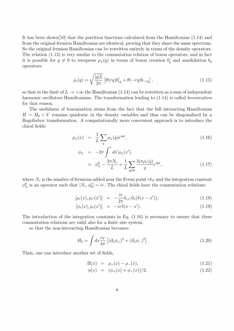
Our aim is to understand the low-energy spectrum of the Hamiltonian (1.5). Since we arerestricting to low energy excitations, it is justified to linearize the spectrum around the twoFermi points ±kF , as shown on the Fig. 1.1. Our Hamiltonian can then be rewritten in termsof left moving (−) and right moving (+) fermions as:
H =∑
k,r
vF rkc†k,rck,r (1.8)
6
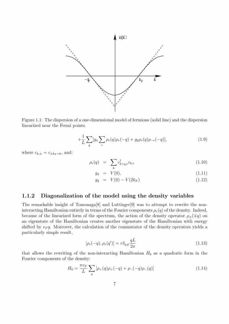
ε( )k
kF−kF k
Figure 1.1: The dispersion of a one-dimensional model of fermions (solid line) and the dispersionlinearized near the Fermi points.
+1
L
∑
q
[g4∑
r
ρr(q)ρr(−q) + g2ρr(q)ρ−r(−q)], (1.9)
where ck,± = c±kF+k, and:
ρr(q) =∑
k
c†k+q,rck,r (1.10)
g4 = V (0), (1.11)
g2 = V (0)− V (2kF ) (1.12)
1.1.2 Diagonalization of the model using the density variables
The remarkable insight of Tomonaga[8] and Luttinger[9] was to attempt to rewrite the non-interacting Hamiltonian entirely in terms of the Fourier components ρr(q) of the density. Indeed,because of the linearized form of the spectrum, the action of the density operator ρ±(∓q) onan eigenstate of the Hamiltonian creates another eigenstate of the Hamiltonian with energyshifted by vF q. Moreover, the calculation of the commutator of the density operators yields aparticularly simple result,
[ρr(−q), ρr(q′)] = rδq,q′qL
2π(1.13)
that allows the rewriting of the non-interacting Hamiltonian H0 as a quadratic form in theFourier components of the density:
H0 =πvFL
∑
q
[ρ+(q)ρ+(−q) + ρ−(−q)ρ−(q)] (1.14)
7
It has been shown[10] that the partition functions calculated from the Hamiltonian (1.14) andfrom the original fermion Hamiltonian are identical, proving that they share the same spectrum.So the original fermion Hamiltonian can be rewritten entirely in terms of the density operators.The relation (1.13) is very similar to the commutation relation of boson operators, and in factit is possible for q 6= 0 to reexpress ρ±(q) in terms of boson creation b†q and annihilation bqoperators:
ρr(q) =
√
|q|L2π
[
θ(rq)b†rq + θ(−rq)b−rq
]
, (1.15)
so that in the limit of L→ +∞ the Hamiltonian (1.14) can be rewritten as a sum of independentharmonic oscillators Hamiltonians. The transformation leading to (1.14) is called bosonization
for that reason.The usefulness of bosonization stems from the fact that the full interacting Hamiltonian
H = H0 + V remains quadratic in the density variables and thus can be diagonalized by aBogoliubov transformation. A computationally more convenient approach is to introduce thechiral fields:
ρ±(x) =1
L
∑
q
ρ±(q)eiqx, (1.16)
φ± = −2π
∫ x
dx′ρ±(x′),
= φ0± − 2πNr
L+
1
L
∑
q 6=0
2iπρr(q)
qeiqx, (1.17)
whereNr is the number of fermions added near the Fermi point rkF and the integration constantφ0± is an operator such that [Nr, φ
r0] = ir. The chiral fields have the commutation relations:
[ρr(x), ρr′(x′)] = − ir
2πδr,r′∂x(δ(x− x′)), (1.18)
[φr(x), ρr(x′)] = −irδ(x− x′). (1.19)
The introduction of the integration constants in Eq. (1.16) is necessary to ensure that thesecommutation relations are valid also for a finite size system.
so that the non-interacting Hamiltonian becomes:
H0 =
∫
dxvF4π
[
(∂xφ+)2 + (∂xφ−)
2]
. (1.20)
Then, one can introduce another set of fields,
Π(x) = ρ+(x)− ρ−(x), (1.21)
φ(x) = (φ+(x) + φ−(x))/2, (1.22)
8
having Fourier decomposition:
Π(x) =J
L+
1
L
∑
q 6=0
[ρ+(q)− ρ−(q)]eiqx, (1.23)
φ(x) =1
2(φ0
+ + φ−0 )−
πNx
L− π
L
∑
q
ρ+(q) + ρ−(q)
iqeiqx, (1.24)
with J = N+ − N− and N = N+ + N−. The fields defined in (1.21) satisfy the canonicalcommutation relation [φ(x),Π(x′)] = iδ(x− x′) and allow the rewriting of the non-interactingHamiltonian in the form:
H0 = vF
∫
dx
2π
[
(πΠ)2 + (∂xφ)2]
, (1.25)
and of the interaction term in the form:
V =
∫
dxg42
(
Π2 +(∂xφ)
2
π
2)
+
∫
dxg22
(
−Π2 +(∂xφ)
2
π
2)
, (1.26)
giving for the full Hamiltonian:
H =
∫
dx
2π
[
uK(πΠ)2 +u
K(∂xφ)
2]
, (1.27)
where:
u2 =(
vF +g4π
)2
−(
2g2π
)2
(1.28)
K =
√
πvF + g4 − 2g2πVF + g4 + 2g2
(1.29)
The Hamiltonian can be brought back to the non-interacting form by a simple rescaling of thefields, φ = φ/
√K and Π =
√KΠ, which is equivalent to the Bogoliubov transformation. In
the form (1.27), the Hamiltonian describes one-dimensional phonons, with a displacement fieldφ(x) and a momentum density Π(x). Indeed, if we consider a one-dimensional harmonic chain,with Hamiltonian:
H =∑
n
[
p2n2m
+k
2(un − un+1)
2
]
, (1.30)
and [un, pm] = iδn,m, calling a the lattice spacing, we can introduce the continuum fieldsP (na) = pn/a and u(na) = un, and obtain the commutation relation [u(x), P (x′)] = iδ(x− x′)with the continuum Hamiltonian:
H =
∫
dx
[
P 2
2ρ+κ
2(∂xu)
2
]
, (1.31)
9
where we have defined ρ = m/a and κ = ka, which is precisely the form (1.27). The analogycan be pushed further by noting that with our definitions, the density ρ(x) = ρ+(x) + ρ−(x) =−∂xφ/π, which corresponds to the usual definition of the density[11] as a function of the dis-placement in elasticity theory, ρ(x) = −∂xu. Following that analogy, we can view bosonizationas a consequence of having particles moving along a line. When a particle is moving, it isforced to interact with its neighbors, and exchange some momentum with them. As a result,the individual motion of a particle is quickly transformed into a collective motion representedby a compression wave.
1.1.3 Expressing the operators in terms of the density variables
Having found the spectrum, the next step is to calculate the correlation functions of the model.In particular, it is useful to determine the fermion Green’s functions. To do that, one canremark that the commutation relations of the density with the fermion annihilation operatorare:
[ρ(x), ψ(x)] = δ(x− x′)ψ(x) (1.32)
Thus, the fermion annihilation operator has the same commutation relation with the densityas the exponential e−irφr(x), and it is expected that ψr(x) ∼ e−irφr(x).
Indeed, the fermion annihilation and creation operators can be written[12, 10]:
ψ+(x) =1√L
: e−iφ+(x) :, (1.33)
ψ−(x) =1√L
: eiφ−(x) :, (1.34)
where : . . . : indicates normal ordering. Using the relations:
[φr(x), ψr(x′)] = iπrδ(x− x′), [φ+(x), φ−(x
′)] = iπ, (1.35)
where the last commutator is a consequence of the choice of commutator [φ0+, φ
0−] = iπ, and
using the Glauber identity eAeB = eA+Be12[A,B] valid for [A, [A,B]] = [B, [A,B]] = 0, one can
check that (1.33) indeed reproduce the commutation relations of the fermion operators.A less rigorous version of (1.33) is obtained keeping the cutoff finite and neglecting the
normal ordering. One can then write:
ψ+(x) =ei(θ−φ)
√2πα
, (1.36)
ψ−(x) =ei(θ+φ)
√2πα
, (1.37)
where we have introduced θ = (φ− − φ+)/2. With (1.36) and , the retardated Green’s functionat T = 0 of right moving fermions is obtained in the form:
G+(x, t) =1
2π(x− ut− i0+)
(
α2
x2 − (ut+ i0+)2
)(√K−1/
√K)2/4
(1.38)
10
taking the Fourier transform of the Green’s function, the spectral function is[13]:
A+(k, ω) =π
Γ(λ)Γ(λ+ 1)
[
(ωα
v
)2
− (qα)2]K−1/K
Θ(ω − vq)Θ(ω + vq)
ω − vq(1.39)
The delta peak at ω = vq is changed into a power-law singularity that indicated that theFermion excitations have become incoherent, the true long lived excitations being the densitymodes (1.16). Also, a threshold is present for ω = −vq which is a sign of the interaction of thetwo Fermi points. The calculation of the momentum distribution shows also that the step at theFermi energy is replaced by a power law singularity n(k) ∼ 1
2+C|k−kF |
12(K+1/K−2)sign(kF −k).
The energy distribution obeys the same law, n(ǫ) ∼ 12+ C|ǫ− ǫF |
12(K+1/K−2)sign(ǫF − ǫ).
For finite temperature, the spectral functions can be derived in a similar manner. TheGreen’s function takes the form:
G+(x, t) =−i2πα
(
πTα
iu sinh πTu(x− ut)
) 14(K+ 1
K+2)(
πTα
−iu sinh πTu(x+ ut)
) 14(K+ 1
K−2)
, (1.40)
Leading to the spectral function[14]:
A+(k, ω) ∼(
πTα
u
) 12(K+K−1)
Re
[
(2i)γB
(
γ
2− i
uq − ω
4πT, 1− γ
)]
Re
[
(2i)γ+1B
(
γ + 1
2− i
uq + ω
4πT,−γ
)]
,
(1.41)where we have defined γ = (K + K−1 − 2)/4. In the case of finite size, the Fermion Green’sfunctions have been obtained at T = 0 as well as for finite temperature[15]. The derivationrequires a more careful treatment of the boundary conditions and of the zero modes than inthe present introduction.
Besides the obtention of the Fermion Green’s function, the Eq. (1.36) also allow us to obtaina more complete representation of the density operator. Indeed, since ψ(x) = eikF xψ+(x) +e−ikF xφ−(x), we can write the density as:
ρ(x) = ψ†(x)ψ(x), (1.42)
=∑
r
ψ†r(x)ψr(x)e
2ikF xψ†−(x)ψ+(x) + e2ikF xψ†
+(x)ψ−(x), (1.43)
= − 1
π∂xφ+
sin(2φ(x)− 2kFx)
πα, (1.44)
Therefore, an oscillating component of the density, of wavevector ±2kF is also present. Thiscomponent is the order parameter for 2kF charge density wave ordering. Using Wick’s theorem,it can be shown that for zero temperature:
〈Tτe2iφ(x,τ)e−2iφ(0,0)〉 = e−2〈Tτ (φ(x,τ)−φ(0,0))2〉(
α2
x2 + (uτ)2
)K
, (1.45)
11
so that no long range order, but only quasi-long range order is possible in the ground state, inagreement with the Mermin-Wagner-Hohenberg theorem.[16, 17, 18] The order parameter for
superconductivity, OSC = ψ+(x)ψ−(x) ∼ e2iθ(x)
2παcan also be considered. One has:
〈Tτei2θ(x,τ)e−2iθ(0,0)〉 =(
α2
x2 + (uτ)2
)1/K
, (1.46)
so that superfluid correlations are also quasi-long range ordered. The superfluid exponent is theinverse of the density wave exponent. This can be understood as the consequence of a dualityproperty. Indeed, the Hamiltonian (1.27) can be rewritten:
H =
∫
dx
2π
[ u
K(πP )2 + uK(∂xθ)
2]
, (1.47)
where ∂xφ = πP . One has the commutation relations [θ(x), P (x′)] = iδ(x − x′) so that theHamiltonian (1.47) can be changed into (1.27) by the substitution θ(x) → φ(x), P (x) → Π(x)and K → 1/K. As a result, the correlations of exponentials of the θ field are obtained from thecorrelation of the φ fields by the substitutionK → 1/K. In general, with the Hamiltonian (1.27)the two-point ground state correlation functions are of the form:
〈Tτeiλφ(x,τ)e−iλφ(0,0)〉 = e−λ2〈Tτ (φ(x,τ)−φ(0,0))2〉/2 =
(
α2
x2 + (u|τ |+ α)2
)λ2K/4
(1.48)
〈eiλθ(x,τ)e−iλθ(0,0)〉 = e−λ2〈Tτ (φ(x,τ)−φ(0,0))2〉/2 =
(
α2
x2 + (u|τ |+ α)2
)λ2K−1/4
(1.49)
In the language of the renormalization group, the operator eiλφ has the scaling dimension λ2K/4while the operator eiλθ has scaling dimension λ2/(4K). An operator ei(αθ+λφ) has a scalingdimension (α2/K + λ2K)/4, but its correlation function also contains a phase factor. TheFourier transform of the correlation functions (1.48) gives the Matsubara response functions.For a general correlation function of the form:
〈TτO(x, τ)O(0, 0)〉 =(
α2
x2 + (uτ)2
)γ
, (1.50)
The Fourier transform is (for γ < 1):
χO(q, iω) =π22(1−γ)Γ(1−γ)
uΓ(γ)α2γ
(
q2 +ω2
u2
)(γ−1)
, (1.51)
giving after analytic continuation iω → ω + i0 the response function. For γ < 1, the responsefunction is divergent. This implies a divergent density-wave response for K < 1 (i. e. repulsiveinteractions) and a divergent superconducting response forK > 1 (i. e. attractive interactions).
For positive temperature, the correlation functions take the form:
12
〈Tτ (φ(x, τ)− φ(0, 0))2〉 = −K2ln
x2 + (u|τ |+ α)2
α2
Γ4(
1 + αβu
)
Γ(
1 + α−izβu
)
Γ(
1 + α+izβu
)
Γ(
1 + α−izβu
)
Γ(
1 + α+izβu
)
(
〈Tτ (θ(x, τ)− θ(0, 0))2〉 = − 1
2Kln
x2 + (u|τ |+ α)2
α2
Γ4(
1 + αβu
)
Γ(
1 + α−izβu
)
Γ(
1 + α+izβu
)
Γ(
1 + α−izβu
)
Γ(
1 + α+izβu
)
(
where β = 1/(kBT ), z = x − iuτ , z = x + iuτ and Γ is the Gamma function[19]. As afunction of Matsubara time, the correlation functions are periodic of period β, as required bythe Kubo-Martin-Schwinger condition[20]. In the limit α ≪ βu, |z|, the expressions (1.52) canbe simplified, using the identity (6.1.17) in [19] yielding the approximate correlation functions:
〈Tτeiλφ(x,τ)e−iλφ(0,0)〉 ≃
π2α2
β2u2 sinh(
πzβu
)
sinh(
πzβu
)
λ2K/4
, (1.54)
〈Tτeiλθ(x,τ)e−iλθ(0,0)〉 ≃
π2α2
β2u2 sinh(
πzβu
)
sinh(
πzβu
)
λ2K−1/4
. (1.55)
For long distances, the correlation functions (1.54) decay exponentially with distance. Thecharacteristic length πu/(kBT ) is the thermal length. The result (1.54) can be derived withconformal field theory[21] by mapping the plane on a cylinder of circumference β. In thatlanguage, the origin of the exponential decay of the correlation functions is the fact that thesystem has the same correlation functions as a quasi-one dimensional system. The responsefunctions corresponding to (1.54) have been obtained[22, 23] from the integral (convergent forγ < 1/2):
Iγ(q, ω) =
∫ +∞
−∞dx
∫ β
0
dτei(qx−ωτ)
∣
∣
∣sinh(
π(x+iuτ)βu
)∣
∣
∣
2γ (1.56)
=β2u sin(πγ)
(2π)2B
(
1− γ,γ
2+β(|ωn|+ iuq)
4π
)
B
(
1− γ,γ
2+β(|ωn| − iuq)
4π
)
The finite temperature response functions are finite for q, ω → 0, however they diverge as apower law of temperature when T → 0.
To summarize that section: We have seen that with spinless fermions in one dimension, thelong-lived low energy excitations are not fermionic quasiparticles as in the three dimensionalcase, but instead are bosonic collective modes analogous to sound waves. These modes aredescribed by a one-dimensional harmonic Hamiltonian. The fermion excitations are incoherent,and the ground state superconducting and density wave correlations have only quasi-long rangeorder, with corresponding power law divergences of the response functions.
13
1.2 The XXZ spin-chain model
1.2.1 Jordan-Wigner transformation and derivation of a bosonizedHamiltonian
The Tomonaga-Luttinger liquid Hamiltonian (1.27) is also applicable to the study of spin-1/2chains. That can be understood by considering the Jordan-Wigner transformation[24]:
S+n = (−)nc†ne
iπ∑
m<n c†mcm , (1.57)
Szn = c†ncn −
1
2, (1.58)
where Sx,y,zn are spin-1/2 operators, S+
n = Sxn + iSy
n, and the cn are fermion annihilation oper-ators. While spin-1/2 operators anticommute on the same site, but commute on different site,fermion operators always anticommute. The Jordan-Wigner operator:
eiπ∑
m<n c†mcm (1.59)
compensates the anticommutation relation of the fermion operators on different sites and thuspermits to reproduce exactly the spin-1/2 operator algebra.
As a result, the Hamiltonian of the XXZ spin chain:
H =∑
n
[
J(SxnS
xn+1 + Sy
nSyn+1) + JzS
znS
zn+1 − hSz
n
]
, (1.60)
is mapped to the t− V model of interacting fermions.
H =∑
n
[
−t(c†n+1cn + c†ncn+1) + V (c†ncn − 1/2)(c†n+1cn+1 − 1/2)− µc†ncn
]
, (1.61)
with t = J/2, V = Jz and µ = h. The phase factor (−)n in (1.57) has been inserted toensure that for V = 0 the minimum of the kinetic energy is at k = 0. In the limit V ≪ t,a bosonized representation of the Hamiltonian (1.61) can be derived. For V = 0, we willhave two Fermi points at ±kF with µ = −2t cos(kFa) where a is the lattice spacing of ourmodel. We can also relate the Fermi wavevector to the magnetization of the XXZ model using:m = 〈Sz〉 = kF/π − 1/2. For h 6= 0, we can take the continuum limit as we did for Eq. (1.5),and we obtain a bosonized Hamiltonian of the for (1.27). For h = 0, a more careful treatmentis required. Indeed, for h = 0, the t− V model is at half-filling and kF = π/(2a) so that:
c†ncn = a
[
∑
r
ψ†rψr + eiπ
xa
∑
r
ψ†rψ−r
]
, (1.62)
and since we have a discrete sum in (1.61), the terms ψ†+ψ
†+ψ−ψ− +H.c. do not drop out from
the Hamiltonian. In more physical terms, when kF = π/(2a), we have 4kF = 2π/a i.e. 4kF is
14
a reciprocal lattice vectors, and interactions can include umklapp terms[25]. Using (1.36), wecan nevertheless derive a bosonized representation of the Hamiltonian (1.61):
H =
∫
dx
2π
[
uK(πΠ)2 +u
K(∂xφ)
2]
− 2V
(2πα)2
∫
dx cos 4φ, (1.63)
Since the scaling dimension of cos 4φ is 4K, this term is irrelevant in the renormalization groupsense as long as K > 1/2. Within the perturbative treatment, K ≃ 1, so the renormalizationgroup fixed point is a still Hamiltonian of the form (1.27) with renormalized parameters u∗ andK∗.
1.2.2 Derivation of a bosonized representation for spin operators
Using the relations (1.57), it is possible to derive a bosonized representation of the spin op-erators. First, we need to use a slightly modified expression of the Jordan-Wigner operatorcompared with (1.59), that has the advantage to yield a hermitian expression in the continuumlimit[26], i. e.
eiπ∑
m<n c†mcm = cos
[
π∑
m<n
c†mcm
]
. (1.64)
On the lattice, the expressions (1.59) and (1.64) are completely equivalent, but (1.64) becomesafter bosonization:
cos(φ− kFx), (1.65)
while (1.59) would give a non-hermitian expression. The reason for such difference is that wehave approximated a field taking only discrete values by a field taking its value in a continuum.Using the bosonized expressions of the fermion operators, we derive a bosonized representationof the spin operators:
S+(x) =S+n
α=eiθ(x)√πα
[
(−)x/a + cos(2φ(x)− 2kFx+ πx/a)]
, (1.66)
Sz(x) =Szn
a= − 1
π∂xφ− 1
παsin(2φ− 2kFx), (1.67)
In the representation (1.66), θ plays the role of an azimuthal angle. To derive (1.67), the Glauberidentity and the commutators (1.35) have been used to express the products ψ†
RψL + H.c.. Itis also possible to derive a bosonized representation of the operator S+
n+1S−n of the form:
S+n+1Sn =
u
2π
[
(πΠ)2 + (∂xφ)2]
+cos(2φ− 2kFx)
πα. (1.68)
Such representation allows us to find the correlation functions of the XXZ spin chain at T = 0and find that it has only quasi-long range order in the vicinity of Jz = 0.
15
1.3 Hard core bosons
Using the Holstein Primakoff representation[27], one can write a spin S operator as:
Szn = b†nbn − S, (1.69)
S+n = b†n
√
2S − b†nbn, (1.70)
with the constraint b†nbn ≤ 2S. For S = 1/2, Eq. (1.69) shows that a spin-1/2 is equivalent toa hard core boson. In particular, the Jordan-Wigner transformation (1.57) can also be usedto represent hard core bosons in terms of fermions.2 The Eqs. (1.66)– (1.67) thus also yield abosonized representation of hard-core bosons. It is important to note that the representationthus obtained is non-trivial. The bosonic modes that enter the problem can be understoodas the density modes of the hard core boson system as we discussed previously for fermions.Hard core bosons can also be considered directly in the continuum [28] and the bosonizedrepresentation that we have derived is also applicable.
Another instructive manner to arrive at the bosonized representation of boson operatorsis by considering the number-phase representation. In that representation, we first considerthe number operator Nn = b†nbn and define its canonically conjugate variable θn such that[Nn, θn] = i. We can then rewrite the boson annihilation operator as bn = eiθn
√Nn and
the boson creation operator as b†n =√Nne
−iθn .3 Taking the continuum limit, we find theannihilation operator in the form ψB(x) = bn/
√α = eiθ
√
ρB(x), where ρB(x) is the bosonicparticle density, and θ(x) is the superfluid phase of the boson field. The commutator becomes[ρ(x), θ(x′)] = iδ(x − x′). This result is also consistent with the form of the order parameterfor superfluidity of the spinless fermions. Moreover, in a model of interacting bosons such asthe Lieb-Liniger model[29]:
H =
∫
dx
[
1
2m∂xψ
†B∂xψB(x)− µψ†
BψB(x) +g
2ψ†Bψ
†BψBψB(x)
]
(1.71)
the number phase representation leads to the Hamiltonian:
H =
∫
dx
[
1
2m
(
(∂xρB)2
4ρB+√ρB(∂xθ)
2√ρB)
− µρB +g
2ρ2B
]
. (1.72)
Minimizing the classical energy with respect to the boson density, we obtain an average bosondensity 〈ρB〉 = µ/g. Replacing in (1.72) the operator ρB by 〈ρB〉δρB and expanding to quadraticorder, we obtain a Hamiltonian:
H =
∫
dx
[
1
2m
(
(∂xδρB)2
4〈ρB〉+ 〈ρB〉(∂xθ)2
)
+g
2(δρB)
2
]
(1.73)
2In that case the phase factor (−)n can be removed, provided that the kinetic energy of the bosons withouthard core interaction is minimal for k = 0
3With that representation, we are actually enlarging the Hilbert space adding an unphysical space whereNn takes negative values. However, the bn operators annihilate the states with Nn = 0, so that no admixturebetween the physical and unphysical Hilbert space can take place when the boson Hamiltonian is normal ordered.
16
Neglecting the (∂xδρB)2 term, the Hamiltonian (1.73) reduces to a Hamiltonian of the form (1.47)
with uK = π〈ρB〉/m, u/K = g/π, δρ = −πP . The Hamiltonian (1.73) yields the same dis-persion relation for the low-energy modes as the Bogoliubov approximation, but does not relyon the incorrect assumption of Bose condensation. If we return to the Hamiltonian (1.71) andderive equations of motion for the fields θ and ρ, we obtain:
∂tρ+ ∂x(ρ∂xθ/m) = 0 (1.74)
∂tθ +(∂xθ)
2
2m=
δ
δρ
(
−µρ+ gρ2/2 + (∂xρ)2/(8mρ)
)
(1.75)
The first equation is the continuity equation, the second one is the Euler equation with velocitypotential θ/m. This shows that bosonization can be viewed as linearized quantum hydrody-namics, and that the linearly dispersing excitations predicted by bosonization can be viewedas sound modes, as already suggested by the one-dimensional phonon analogy (1.30). In thispicture, we can view the Tomonaga-Luttinger liquid as a one-dimensional crystal melt by quan-tum fluctuations. Such hydrodynamic interpretation is independent of particle statistics. Whenconsidering the picture obtained from the phase representation, we can alternatively view theTomonaga-Luttinger liquid as a superfluid whose long range order is turned into quasi-longrange order by quantum fluctuations. Thus, the absence of ordering breaking the continuousU(1) translation symmetry and U(1) global gauge symmetry appears to place one-dimensionalsystems of interacting particles in a kind of “fluctuating supersolid” state, with both quasi-longrange crystalline and superfluid order.
1.4 The Tomonaga-Luttinger liquid concept
Until now, we have discussed the solution of the Tomonaga-Luttinger model within a perturba-tive framework. However, it has been argued by Luther[30] and Haldane[31] that the bosonizedHamiltonian offered a more general description of the low energy physics of interacting parti-cles in one-dimension than suggested by the perturbative treatment. Indeed, the theoreticaltreatment shows that the Tomonaga-Luttinger model is scale invariant, and can be viewedas a renormalization group fixed point[6]. This suggests that the Hamiltonian can be viewedin general as the fixed point Hamiltonian of a gapless model of interacting particles. Such afixed point is characterized by two parameters, the velocity of excitations and the Luttingerparameter. The fixed point is called the Tomonaga-Luttinger liquid. In a more modern lan-guage, one would note that a model in which the low energy dispersion of excitation is linearis at a renormalization group fixed point with a dynamical exponent z = 1. For such a fixedpoint, space and rescaled Matsubara time are equivalent, and as a result, the scale invarianceof the fixed point implies the full conformal invariance of the model.[32] Conformal field theoryallows for a classification of the conformally invariant fixed points. Since the model has U(1)symmetry, a plausible fixed point is the c = 1 conformal field theory generated by the U(1)Katz-Moody algebra the Hamiltonian of which is precisely (1.27). The interpretation of K inthe language of conformal field theory is simply that K is the compactification radius of theconformal field theory. From a practical point of view, in order to characterize a system in
17
the Tomonaga-Luttinger liquid state, one has to determine the velocity of excitations and theTomonaga-Luttinger parameter from the macroscopic observables. A simple approach is tocalculate the charge (or spin) stiffness and the compressibility with the help of the fixed pointHamiltonian and relate them with the exact quantities. First, if we consider the compressibil-ity, with the help of (1.23), we see that adding one particle to our system is going to makeφ(x) → −πx/L. Using the Hamiltonian (1.27), we see that this is going to shift the energy bythe amount πu/(2KL). If we consider the ground state energy change, since in an extensivesystem the ground state energy E0(N,L) − µN behaves as: E0(N,L) = Le(N/L) − µN , wefind that the ground state energy changes by: e′(N/L) − µ + e”(N/L)/(2L), so that, sincee′(N/L) = µ, we have:
e”(N/L) =πu
K(1.76)
Using the definition of the compressibility as:
κ = − 1
L
(
∂L
∂P
)
N
(1.77)
= − 1
ρ0(∂P/∂ρ0), (1.78)
where the pressure P = −(∂E0/∂L)N , we find that κ = 1/(ρ20e”(ρ0)) = K/(πuρ20). Now, if weturn to the stiffness, we have to consider our system under a change of boundary conditionssuch that ψ(L) = eiϕψ(0). Such a change of boundary condition amounts to making θ(x) →θ(x) + ϕx/L giving a shift of the ground state energy from (1.27) equal to uKϕ2/(2πL). Thisgives us the second relation:
πL∂2E0
∂2ϕ= uK. (1.79)
In the case of a Galilean invariant model, the relation (1.79) can be further simplified.Indeed, under a Galilean boost, ψ(x, t) → eimvx−mv2t/2ψ(x, t) so that θ(x, t) → θ(x, t) +mvx−mv2t/2 and πΠ → πΠ+mv. In the Hamiltonian (1.27), this gives a shift of the energy equal touK(mv)2L/(2π). But in a Galilean invariant model, the energy is simply shifted by Nmv2/2in the moving frame. Equating the two quantities, we find that uK = πN/(mL) i. e.
uK =πρ0m
. (1.80)
Such an approach has been applied to the t − V model (or equivalently the XXZ chain)of Eq. (1.61) by Haldane. The t − V model is integrable by the Bethe Ansatz (BA), andthe low energy spectrum as well as the stiffness and the compressibility can be obtained non-perturbatively. The Tomonaga-Luttinger theory then fixes relation between the velocity ofexcitations u, the compressibility and the stiffness which have been checked on the BA solution.For h = 0, an analytic expression of u,K is available:
K =1
2− 2πarccos V
2t
u = π
√
t2 − V 2
4
arccos(
V2t
) (1.81)
18
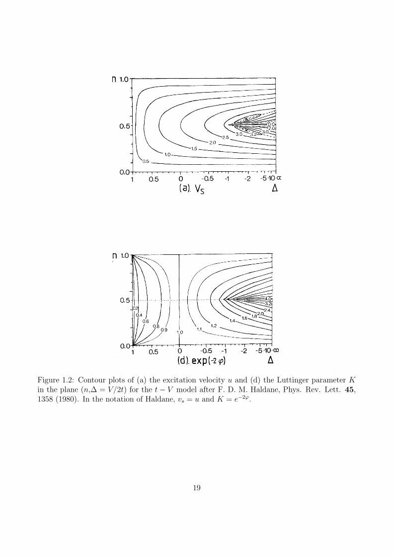
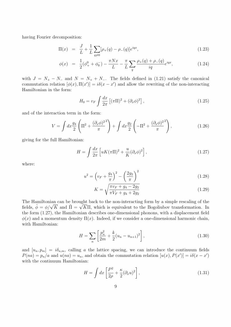
Figure 1.2: Contour plots of (a) the excitation velocity u and (d) the Luttinger parameter Kin the plane (n,∆ = V/2t) for the t − V model after F. D. M. Haldane, Phys. Rev. Lett. 45,1358 (1980). In the notation of Haldane, vs = u and K = e−2ϕ.
19
which becomes in the case of the XXZ chain:
K =1
2− 2πarccos Jz
J
u =π√
J2 − J2z
2 arccos(
JzJ
) (1.82)
These expressions are defined only for |Jz| < J (or |V | < 2t in the t− V model). For Jz < −J ,the XXZ chain has a ferromagnetic long range order, and for Jz > J it has an antiferromagneticlong range order. The phase transitions from the Luttinger liquid state to the ferromagnet andto the antiferromagnet belong to different universality classes. In the case of the transitionto the ferromagnetic state, the Luttinger exponent is diverging at the transition, while thevelocity is vanishing[33, 34]. On the ferromagnetic side, the dispersion of excitations is gaplessand quadratic. In the case of the transition to the antiferromagnetic state, both the velocityand the Luttinger exponent remain finite at the transition, but the excitations become gapful onthe antiferromagnetic side. The latter type of transition belong to the Berezinskii-Kosterlitz-Thouless[35, 36] to be discussed in chapter 2. For now, let us just note that for J = Jzthe scaling dimensions of the operators eiθ and cos 2φ, as well as eiθ cos 2φ and ∂xφ in (1.66)and (1.67) become respectively 1/2 and 1, as we would expect from SU(2) invariance. Thequantities u,K have also been derived for the Lieb-Liniger model.[37] They only depend on thedimensionless parameter γ = mg/ρ0. For γ ≪ 1, their behavior follows the prediction fromthe Bogoliubov approximation (1.73). For γ → ∞, the bosons behave as hard core bosons andK → 1, u → πρ0/m. There are two ways to reach that limit, the first one is by sending g toinfinity, the second one is by sending the density to zero.
The Tomonaga-Luttinger exponent has also been obtained for the non-integrable Bose-Hubbard model[38].
Besides knowing the expression of the fixed point bosonized Hamiltonian, we also need arepresentation of the density and particle creation and annihilation operators in terms of thefields that enter the Hamiltonian (1.27). Haldane[39] proposed the following arguments tojustify such a representation.
First, we will consider classical particles along a line, and call xm the positions of theparticles. We will then define a field φ(x) such that φ(xm) = mπ and φ(x) is an increasingfunction of x. The particle density will then be given by
ρ(x) =∞∑
m=−∞δ(x− φ−1(mπ)), (1.83)
=∞∑
m=−∞δ(φ(x)−mπ)
dφ
dx, (1.84)
=1
π
∞∑
k=−∞e2ikφ(x)
dφ
dx, (1.85)
where in the last line we have applied the Poisson summation formula. For a given averagedensity of particles ρ0, there are ρ0x particles between the position 0 and the position x > 0,
20
so we expect that φ(x) = πρ0x− φ(x), yielding:
ρ(x) =
(
ρ0 −1
π∂xφ
) ∞∑
k=−∞e2ik(πρ0x−φ(x)). (1.86)
That formula is analogous to the formula giving the particle density in Eq. (1.42). It is assumedthat for the quantum system, a similar formula holds, with:
ρ(x) = ρ0 −1
π∂xφ+
∑
m
Ame2im(φ(x)−2πρ0x). (1.87)
The coefficients Am cannot in general be predicted from bosonization as they depend on thedetails of the model. In perturbative bosonization, only the terms A±1 are nonzero. The originof the higher order terms can be understood by the following argument.
The 4kF component of the density is given by an operator ρ(4kF ) =∑
q c†kF+qc−3kF+q. In
first order perturbation theory, the ground state of the interacting system is given by:
|0〉+ V (2kF − q − q′)
ǫ(3kF − q′) + ǫ(kF − q′)− ǫ(kF − q)− ǫ(kF + q)c†−3kF+q′c
†kF−q′c−kF+qc−kF+q|0〉+ . . . ,(1.88)
Acting on that state with ρ(4kF ) and neglecting approximating ǫ(nkF + q) ∼ ǫ(nkF ), V (2kF +q) ∼ V (2kF ) yields a contribution proportional to:
ρ(4kF ) ∼V (2kF )
ǫ(3kF )− ǫ(kF )
∑
q,q′
c†kF+q′c†kF−q′c−kF+qc−kF+q (1.89)
(1.90)
the bosonized expression of which is:
ρ4kF (x) ∼V (2kF )
ǫ(3kF )− ǫ(kF )e4i(φ(x)−πρ0x) (1.91)
Turning to the expression of the particle annihilation operator, one can start from the phaserepresentation (1.72) encountered, with:
ψB(x) = eiθ(x)√
ρ(x) (1.92)
It is of course difficult to define properly the square root of an operator which is a sum of deltafunctions. However, since ρ(x) is a periodic function of φ(x), the square root should preservethat property. This leads to the representation:
ψB(x) = eiθ(x)
[ ∞∑
m=−∞Bme
i2m(φ(x)−πρ0x)
]
, (1.93)
21
where again the parameters Bm are not universal. In the perturbative approach, only B0 andB1 are nonzero. With the help of the Jordan-Wigner transformation (1.57), the correspondingrepresentation for fermions is:
ψF (x) = eiθ(x)
[ ∞∑
m=−∞Bme
i(2m+1)(φ(x)−πρ0x)
]
, (1.94)
The non-universal amplitudes have been computed for the XXZ spin chain[40]. One has:
σ+n = eiθ
(−)n√
A
2+
√
A
2cos 2φ+ . . .
(1.95)
σzn = − 1
π∂xφ+ (−)n
√
Az
2cos 2φ+ . . . (1.96)
with:
A =2K2
(2K − 1)2
[
Γ(
14K−2
)
2√πΓ(
K2K−1
)
] 12K
exp
[
−∫ ∞
0
dt
t
(
sinh(
t2K
)
sinh t cosh(
1− 12K
)
t− e−2t
2K
)]
(1.97)
A =8K2
2K − 1
[
Γ(
14K−2
)
2√πΓ(
K2K−1
)
]2K+ 12K
(1.98)
× exp
[
−∫ ∞
0
dt
t
(
cosh(
tK
)
e−2t − 1
2 sinh t2K
sinh t cosh(
1− 12K
)
t+
1
sinh t2K
−(
2K +1
2K
)
e−2t
)]
Az =8
π2
[
Γ(
14K−2
)
2√πΓ(
K2K−1
)
]2K
exp
[
−∫ ∞
0
dt
t
(
sinh(
1K− 1)
t
sinh t2K
cosh(
1− 12K
)
t− 2(1−K)e−2t
)]
(1.99)
The expressions of the higher order terms can be found in [40]. The amplitudes in (1.97) aredivergent in the limit K = 1/2. This is an indication of the presence of logarithmic correctionsto the correlation functions in the SU(2) symmetric case.[41] We will defer their discussion toChapter 2.
1.5 Multicomponent systems
1.5.1 The case of fermions with spin
Derivation of the bosonized Hamiltonian
In the case of non-interacting fermions with spin, we can separately obtain a boson representa-tion of the type (1.36) of the spin up and spin down fermions, with two separate Hamiltonians
22
of the form (1.27) for each spin. However, when considering a Hubbard type interaction:
Hint = g
∫
dxρ↑(x)ρ ↓ (x) (1.100)
= g
∫
dx
[
− 1
π∂xφ↑ +
cos(2φ↑ − 2kF,↑x)
πα
] [
− 1
π∂xφ↓ +
cos(2φ↓ − 2kF,↓x)
πα
]
,(1.101)
when kF,↑ = kF,↓, we note that there is an extra term in the Hamiltonian, of the form:
cos 2(φ↑ − φ↓) (1.102)
Also, when kF,↑ + kF,↓ = 2π/a in a system of spin-1/2 fermions on a lattice (of lattice spacinga) a term of the form:
cos(φ↑ + φ↓) (1.103)
is present in the Hamiltonian.Introducing the new canonically conjugate operators,
φρ =φ↑ + φ↓√
2,Πρ =
Π↑ +Π↓√2
, (1.104)
φσ =φ↑ − φ↓√
2,Πσ =
Π↑ − Π↓√2
, (1.105)
it is possible to rewrite the Hamiltonian in the form:
H = Hρ +Hσ, (1.106)
Hρ =
∫
dx
2π
[
uρKρ(πΠρ)2 +
uρKρ
(∂xφρ)2
]
, (1.107)
Hσ =
∫
dx
2π
[
uσKσ(πΠσ)2 +
uσKσ
(∂xφσ)2
]
− 2g1⊥(2πα)2
∫
dx cos√8φσ, (1.108)
in which the charge excitations (ρ) and the spin excitations (σ) are decoupled. We note thatcos
√8φρ and cos
√8φσ are marginal perturbations in the vicinity of the non-interacting point.
We will defer the renormalization group treatment to a later section, but we already note that amarginally irrelevant operator can give rise to logarithmic corrections to the power-law behaviorof the correlation functions. It should be noted that by the rescaling φσ =
√2φ, θσ = θ/
√2
and Kσ = 2K, the bosonized spin Hamiltonian is mapped on the spin chain Hamiltonian.
Derivation of the bosonized expression of the operators
The fermion creation and annihilation operators take the form:
ψr,σ =e
i√2[θρ−rφρ+σ(θσ−rφσ)]
√2πα
ησ, (1.109)
23
where the operators ησ are Majorana fermion operators with the anticommutation relationησησ′ + ησ′ησ = δσσ′ . It is necessary to introduce the operators to ensure the anticommutationof fermion operators of opposite spins.4 With Eq. (1.109), it is possible to rewrite the chargeand spin density in the form:
ρ(x) =∑
r,σ
ψ†r,σψr,σ (1.110)
= −√2
π∂xφρ +
2
παcos(
√2φρ − 2kFx) cos
√2φσ (1.111)
σ+(x) =∑
r
ψ†r,↑ψr,↓ (1.112)
=ei
√2(θσ−φσ)
2παη↑η↓ +
ei√2(θσ−φσ)
2παη↑η↓ + ei
√2θσ cos(
√2φρ − 2kFx)η↑η↓ (1.113)
σz(x) =1
2
∑
r,σ
σψ†r,σψr,σ (1.114)
= − 1
π√2∂xφσ +
2
παcos(
√2φρ − 2kFx) sin
√2φσ (1.115)
Using the rescaling θσ =√2φ, θσ = θ/
√2, the expressions of the spin density can be brought to
a form reminiscent of Eqs. (1.66)–(1.67). The difference between the two expressions is coming
from the factor ei2kF x−√2φρ . In the case of lattice fermions at half filling kF = π/2a and a charge
gap opens for repulsive interactions giving 〈φρ〉 = 0 , so that the expression (1.112) becomesidentical to the bosonized representation of the spin chain. In that way, the equivalence betweena system of spin-1/2 fermions with a Mott gap and an antiferromagnet is recovered. When thesystem is not at half filling, the presence of the operator φρ is the expression (1.112) is anindication that the carriers of the magnetic moments can have a fluctuating position[43, 44]when charge degrees of freedom are not frozen.
If we consider the spin-spin correlation functions, we observe that the scaling dimensions ofthe operators forming the uniform and staggered parts of σ+ and σz are identical only whenKσ = 1, so that Kσ = 1 is a necessary condition for spin rotational invariance. This conditioncorresponds to K = 1/2 in the XXZ spin-1/2 chain, in agreement with Eq. (1.82). As a result,in a case with SU(2) invariance, only 3 parameters uρ, Kρ and uσ have to be determine todefine non-perturbatively the fixed point bosonized Hamiltonian. For the Hubbard model,these parameters have been determined from the Bethe Ansatz[45]. It has been shown thatKρ > 1/2 for any U .
In the case of a non-integrable model such as the extended Hubbard model at quarter filling,the Tomonaga-Luttinger parameters have been obtained from numerical computation[46].
4Actually, Eq. (1.109) is not a fully rigorous representation. A more correct treatment would use operatorsthat change the fermion number[31, 42], of which the Majorana fermion representation is only an approximation.
24
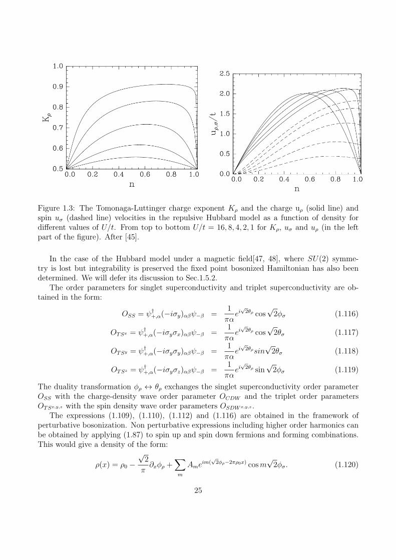
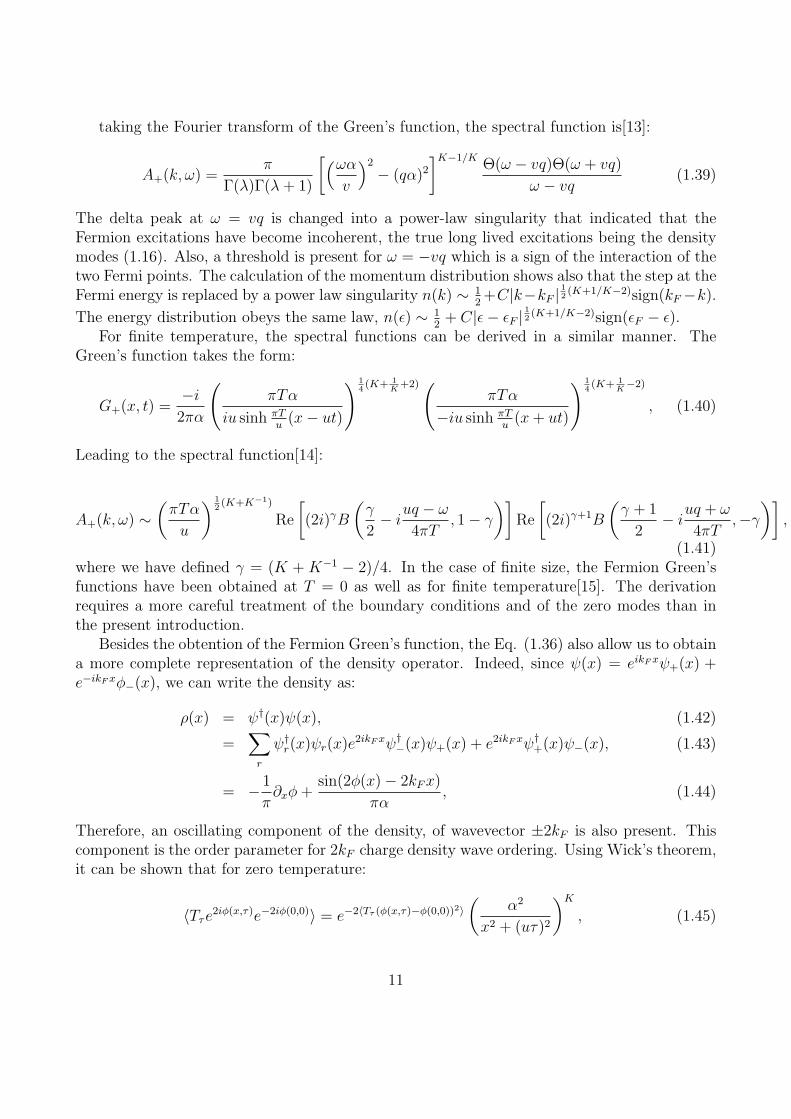
Figure 1.3: The Tomonaga-Luttinger charge exponent Kρ and the charge uρ (solid line) andspin uσ (dashed line) velocities in the repulsive Hubbard model as a function of density fordifferent values of U/t. From top to bottom U/t = 16, 8, 4, 2, 1 for Kρ, uσ and uρ (in the leftpart of the figure). After [45].
In the case of the Hubbard model under a magnetic field[47, 48], where SU(2) symme-try is lost but integrability is preserved the fixed point bosonized Hamiltonian has also beendetermined. We will defer its discussion to Sec.1.5.2.
The order parameters for singlet superconductivity and triplet superconductivity are ob-tained in the form:
OSS = ψ†+,α(−iσy)αβψ−β =
1
παei
√2θρ cos
√2φσ (1.116)
OTSx = ψ†+,α(−iσyσx)αβψ−β =
1
παei
√2θρ cos
√2θσ (1.117)
OTSy = ψ†+,α(−iσyσy)αβψ−β =
1
παei
√2θρsin
√2θσ (1.118)
OTSz = ψ†+,α(−iσyσz)αβψ−β =
1
παei
√2θρ sin
√2φσ (1.119)
The duality transformation φρ ↔ θρ exchanges the singlet superconductivity order parameterOSS with the charge-density wave order parameter OCDW and the triplet order parametersOTSx,y,z with the spin density wave order parameters OSDWx,y,z .
The expressions (1.109), (1.110), (1.112) and (1.116) are obtained in the framework ofperturbative bosonization. Non perturbative expressions including higher order harmonics canbe obtained by applying (1.87) to spin up and spin down fermions and forming combinations.This would give a density of the form:
ρ(x) = ρ0 −√2
π∂xφρ +
∑
m
Ameim(
√2φρ−2πρ0x) cosm
√2φσ. (1.120)
25
However, this expression must be corrected to take into account the presence of the termcos
√8φσ. In perturbative expansions, powers of this term cancel the cos 2m
√2φσ in (1.120)
leading to the corrected expression:
ρ(x) = ρ0 −√2
π∂xφρ +
∑
m
A′2m+1e
i(2m+1)(√2φρ−2πρ0x) cos
√2φσ +
∑
m
A′2me
i2m(√2φρ−2πρ0x)(1.121)
Concerning the spin density, a similar procedure leads to:
S+(x) ∼ ei√2θσ∑
m
A2m+1,xei(2m+1)(
√2φρ−2kF x)
+ei√2θσ cos
√2φσ
∑
m
A2m,xei2m(
√2φρ−2kF x). (1.122)
Sz(x) = − 1
π√2∂xφσ
∑
m
A2m,z sin 2m(√2φρ − 2kFx)
+∑
m
A2m+1,z sin√2φσ sin(2m+ 1)(
√2φρ − 2kFx). (1.123)
It should be noted that in the limit of U/t → +∞, in the Hubbard model, the spins upand down cannot occupy the same site. The charge density is then the same as the one of asystem of spinless fermions having a density equal to the sum of the density of spins up andspins down. Meanwhile, the spin excitations become highly degenerate with a vanishing uσ. Asa result, although the total charge excitations can still be described by bosonization, the spinexcitations require a completely different description. Such limit is called the spin-incoherentTomonaga-Luttinger liquid.[49, 50, 51] and requires a special treatment.
Correlation functions
The ground state response functions for the case of general Kρ and Kσ have been obtained in[52] in terms of the Appell generalized hypergeometric function of two variables F1.[53] Startingfrom the general correlation function:
〈TτO(x, τ)O(0, 0)〉 =
(
α2
(x2 + (uρτ)2
)ηρ ( α2
(x2 + (uστ)2
)ησ
, (1.124)
the Feynman identity[54]:
1∏n
j=1Aαj
j
=Γ(
∑
j αj
)
∏
j Γ(αj)
∫ n∏
j=1
dujuαj−1j
δ(
1−∑j uj
)
(
∑nj=1 ujAj
)−∑
j αj, (1.125)
is used to rewrite the Fourier transform of the Matsubara correlation function (1.124) in theform:
χO(q, ω) =
∫
dxdτ
∫
dvvηρ−1(1− v)ησ−1 α2(ηρ+ησ)eiqx−ωτ
(
x2 + vu2ρτ2 + (1− v)u2στ
2)ηρ+ησ
, (1.126)
26
leading with the help of (1.51) to:
χ(q, ω) =π22(1−ηρ−ησ)α2(ηρ+ησ)Γ(1−ηρ−ησ)
Γ(ηρ + ησ)u2(ηρ+ησ−1)σ
(ω2 + u2σq2)ηρ+ησ−1
×F1
(
ηρ; ηρ + ησ − 1/2, 1− ηρ − ησ; ηρ + ησ, 1− u2ρ/u2σ,
(u2σ − u2ρ)q2
ω2 + u2σq2
)
(1.127)
After analytic continuation, power-law singularities appear in the response function for ω = uσqand ω = uρq. Such singularities mark the presence of a spin and a charge continuum.
In the ground state, and for the spin-isotropic case of Kσ = 1, the spectral functions canbe expressed in terms of the Gauss hypergeometric functions[55]. In the case uρ > uσ and withγρ = (Kρ +K−1
ρ − 2)/8 we have for ω > uρq
A+,s(q, ω) =α2γρ
Γ(γρ)Γ(γρ + 1)
(ω + uρq)γρ(ω − uσq)
γρ−1
(2uρ)γρ+1/2(uρ + uσ)γρ−1/2 2F1
(
1− γρ, γρ +1
2; γρ + 1;
uρ − uσ2uρ
ω + uρq
ω − uσq
)
,
(1.128)
for uσq < ω < uρq,
A+,s(q, ω) =α2γρ
Γ(1/2)Γ(2γρ + 1/2)
(ω + uρq)−1/2(ω − uσq)
2γρ−1/2
(uρ + uσ)γρ−1/2(uρ − uσ)γρ+1/2 2F1
(
1
2, γρ +
1
2; 2γρ +
1
2;
2uρuρ − uσ
ω − uσω + uρ
(1.
and for ω < −uρq,
A+,σ(q, ω) =α2γρ
Γ(γρ)Γ(γρ + 1)
|ω − uσq|γρ−1|ω + uρq|γρ(uρ + uσ)γρ−1/2(2uρ)γρ+1/2 2
F1
(
1− γρ, γρ +1
2; γρ + 1;
uρ − uσ2uρ
ω + uρq
ω − uσq
)
.
(1.130)
In the articles [56, 57], we expressed the spectral functions of the general two-component modelin terms of Appell F2 and F1 functions.
For 0 < uσq < ω < uρq, the spectral function is expressed as:
As(kF,s + q, ω)|uσq<ω<uρq =(α/∆u)νs−1(|ω| − uσq)
νs,ρ+ν′s,σ+ν′s,ρ−1(−|ω|+ uρq)νs,σ+ν′s,σ+ν′s,ρ−1
Γ(νs,ρ + ν ′s,ρ + ν ′s,σ)Γ(νs,σ)(|ω|+ uρq)ν′s,ρ(|ω|+ uσq)
ν′s,σ
× F1
(
νs − 1; ν ′s,ρ, ν′s,σ; νs,ρ + ν ′s,ρ + ν ′s,σ;
2uρ(|ω| − uσq)
∆u(|ω|+ uρq),2u(|ω| − uσq)
∆u(|ω|+ uσq)
)
, (1.131)
and for ω > uρq, as:
As(kF,s + q, ω)|ω>uρq =(α/2uρ)
νs−1(|ω| − uρq)νs,σ+ν′s,ρ+ν′s,σ−1(|ω|+ uρq)
νs,ρ+νs,σ+ν′s,σ−1
Γ(νs,ρ + νs,σ)Γ(ν ′s,ρ + ν ′s,σ)(|ω| − uσq)νs,σ(|ω|+ uσq)ν′s,σ
×F2
(
νs − 1; νs,σ, ν′s,σ, νs,ρ + νs,σ, ν
′s,ρ + ν ′s,σ;
∆u(|ω|+ uρq)
2uρ(|ω| − uσq),∆u(|ω| − uρq)
2uρ(|ω|+ uσq)
)
,(1.132)
27
where u = uρ+uσ, ∆u = uρ−uσ > 0, νs,β = (√
Kβ −1/√
Kβ)2/8, ν ′s,β = (
√
Kβ +1/√
Kβ)2/8,
νs =∑
β(νs,β + ν ′s,β) and F1(α; β, β′; γ; x, y) and F2(α; β, β
′; γ, γ′; x, y) are respectively the firstand second Appell hypergeometric functions [53]. For ω < 0 the spectral function for −uρq <ω < −uσq and for ω < −uρq is obtained by interchanging (1.131) and (1.132) respectively [56].We find As(kF,s+ q, ω) = 0 for |ω| < uσq. The singularities of the spectral functions[58, 59] canbe recovered from these expressions. We have:
AR,s(q, ω) ∝
|ω − uρq|βs,ρ (for ω → +uρq ± 0)(ω − uσq)
βs,σ (for ω → +uσq + 0)(ω + uσq)
β′s,σ (for ω → −uσq − 0)
C + |ω + uρq|β′s,ρ (for ω → −uρq ± 0)
, (1.133)
where
βs,ρ ≡ 1
8(Kρ +K−1
ρ + 2Kσ + 2K−1σ − 2)− 1, (1.134)
βs,σ ≡ ,1
8(2Kρ + 2K−1
ρ +Kσ +K−1σ − 2)− 1 (1.135)
β′s,σ ≡ 1
8(2Kρ + 2K−1
ρ +Kσ +K−1σ + 2)− 1, (1.136)
β′s,ρ ≡ 1
8(Kρ +K−1
ρ + 2Kσ + 2K−1σ + 2)− 1, (1.137)
We have β′s,ρ/σ > 0, so that the singularities for ω = −uρ,σq are cusp singularities, while βs,ρ/σ =
β′s,ρ − 1/2. For weak interactions, the singularities at ω = +uρ,σq are peak singularities, and
turn into cusp singularities for stronger interaction. For finite temperature, spectral functionsand response functions have been expressed as convolution integrals in [14] but no closed formexpression is known in the general case. The integrals giving the spectral functions have beenconsidered numerically in [60].
1.5.2 General multicomponent models
Bosonization is of course also applicable to multicomponent models. Such models can beencountered for instance in ladder or nanotube systems (that will be discussed later) or inKugel-Khomskii models.[61] In the case where all densities are incommensurate, the low-energyHamiltonian takes the form:
H =
∫
dx
2π
∑
a,b
[
π2MabΠaΠb +Nab∂xφa∂xφb
]
, (1.138)
with [φa(x),Πb(x′)] = iδabδ(x − x′). In (1.138) the matrices M and N are real symmetric and
are defined in terms of the variations of the ground state energy EGS of a finite system of sizeL from (respectively) change of boundary conditions ψa(L) = eiϕaψa(0) and change of particledensities ρa = Na/L:
Mab = πL∂2EGS
∂ϕa∂ϕb
, (1.139)
28
Nab =1
πL
∂2EGS
∂ρa∂ρb. (1.140)
The fields φa and θa have the decomposition:
φa(x) = φ(a)0 − πNa
Lx+
1√L
∑
q 6=0
φa(q)eiqx
θa(x) = θ(a)0 − πJa
Lx+
1√L
∑
q 6=0
θa(q)eiqx (1.141)
where πΠa(x) = ∂xθa, [φa(q), θa(−q′)] = −δabδq,q′/q, [φ(a)0 , Jb] = −iδab and [θ
(a)0 , Nb] = −iδab.
The spectrum of the general bosonized Hamiltonian (1.138) is obtained by a linear transformation[62]of the fields Πa and φa:
Πb =∑
β
PbβΠβ, (1.142)
φa =∑
α
Qaαφα, (1.143)
where P tQ = 1 in order to preserve the canonical commutation relations.[63] The matrices Pand Q are calculated explicitly by applying a succession of linear transformations. We define therotation matrix R1 that diagonalizes M , i. e. tR1MR1 = ∆1 with ∆1 a diagonal matrix, andthe matrix N1 = tR1NR1. Since the matrix ∆
1/21 N1∆
1/21 is symmetric, it can be diagonalized
by a second rotation R2, i.e. ∆1/21 N1∆
1/21 = R2∆2
tR2 with ∆2 a second diagonal matrix. Thetransformations P and Q are then:
P = R1∆−1/21 R2(∆2)
1/4, (1.144)
Q = R1∆1/21 R2(∆2)
−1/4, (1.145)
and we have: tPMP = (∆2)1/2 and tQNQ = (∆2)
1/2, giving the transformed Hamiltonian:
H =
∫
dx
2π
[
π2 tΠ(∆2)1/2Π+ t(∂xφ)(∆2)
1/2(∂xφ)]
. (1.146)
In this last equation, the elements on the diagonal of (∆2)1/2 are the velocities uβ of the
decoupled modes of the Hamiltonian (1.138).The definition (1.144) implies in particular that: tPMNQ = ∆2 i.e. Q−1MNQ = ∆2, and
by taking the transpose, P−1NMP = ∆2.The stability of the multicomponent TL liquid state requires that all the velocities are real,
i.e., that the matrix MN has only positive eigenvalues.With the notations of [47, 48], the matrices P and Q are Q = U−1Z, P = tU t(Z−1) where:
U =
(
1 10 1
)
, (1.147)
29
and:
Z =
(
Zcc Zcs
Zsc Zss
)
. (1.148)
The result (1.146) implies that the correlation functions of operators ei∑
a(λaφa+µaθa) can befactorized into products of correlators. We have for zero temperature:
〈Tτei∑n
a=1(λaφa+µaθa)(x,τ)ei∑n
a=1(λaφa+µaθa)(x,τ)〉 = (1.149)n∏
β=1
∏
r=±
(
α
α + uβτ + irx
)2∆(r)β
, (1.150)
where:
2∆(r)β =
1
4
[
n∑
a=1
µaPaβ + rλaQaβ
]2
. (1.151)
Further details can be found in the articles [64, 56, 65].
30
Chapter 2
The sine-Gordon model
Until now, we have deferred the discussion of the sine-Gordon Hamiltonian that was obtainedin systems with umklapp processes or with spin degrees of freedom. In the present chapter,we wish to review the main important results on the sine-Gordon model. We will write thesine-Gordon model in the form:
H =
∫
dx
2π
[
uK(πΠ)2 +u
K(∂xφ)
2]
− 2g
(2πα)2cos
√8φ, (2.1)
which is the one appropriate for the spin sector of the Hubbard model in one dimension. Forthe XXZ spin chain, the bosonized Hamiltonian can be brought to the form (2.1) by a rescalingof the fields. In the case of a dimerized spin-1/2 chain[66] one has to rescale φ → φ/
√2. The
case of the spin chain in staggered field along x can also be reduced to (2.1) by a dualitytransformation.
Classically, the sine-Gordon model is integrable, and the solution of the sine-Gordon equa-tions of motion can be described in terms of solitons, antisolitons and breathers[67]. At theclassical level, the ground state of the sine Gordon Hamiltonian is given by φ = nπ/
√2 with n
integer. A soliton interpolates between the ground state with φ = nπ/√2 at−∞ and the ground
state with φ = (n+1)π/√2 at +∞, while an antisoliton interpolates between φ = (n+1)π/
√2
at −∞, and φ = nπ/√2 at +∞. Breathers are bound states of solitons and antisolitons. All
these excitations have a relativistic-like dispersion E =√
u2p2 +∆2, where ∆ is the mass ofthe excitation and p its momentum. In the classical case, the parameter K plays no role. Bycontrast, in the quantum case, the parameter K is important. As the renormalization grouptreatment will show, the parameter K determines whether the quantum sine-Gordon modelis gapful or gapless. Moreover, in the gapful case, the parameter K also determines whichexcitations are present and how these excitations scatter.
31
2.1 Renormalization group approach
2.1.1 The operator product expansion approach
A very convenient method for deriving RG equations is the operator product expansion technique.[68]The Hamiltonian is written:
H = H0 +∑
i
gi
∫
dxdτOi(x, τ), (2.2)
where H0 is the fixed point Hamiltonian and Oi is an operator of scaling dimension di i. e.
〈Oi(x, τ)Oi(0, 0)〉H0 =
(
α2
x2 + (uτ)2
)di
, (2.3)
where α is a real space cutoff and u is a velocity. The evolution operator in Matsubara time iswritten:
U = exp
[
−∑
i
gi
∫
dxdτOi(x, τ)
]
, (2.4)
and we want to determine how the coupling constants gi will change under a rescaling of thereal space cutoff α → αedℓ. The idea of the method is to consider the product of two normalordered operators Oi(z) and Oj(z
′). The product can be expanded as:
Oi(x, τ)Oj(0, 0) =∑
k
ϕkij(x, τ)Ok(0, 0) + regularterms, (2.5)
Then, if one expands the Matsubara evolution operator (2.4) to second order in the inter-actions, and change the cutoff, a correction to the coupling constants gk will be generated bythe integration over distances α2 < x2 + (uτ)2 < α2e2dℓ. That step gives:
δgk = −1
2
∑
i,j
∫
α2<x2+(uτ)2<α2e2dℓdxdτϕk
ij(x, τ)gjgk, (2.6)
= −πdℓ∑
i,j
Ckijgigj, (2.7)
where we have defined:
Ckij = α2
∫
dθ
2πϕ(α cos θ, α sin θ/u) (2.8)
The second step is a rescaling of the fields to restore the original cutoff. Under the rescaling,gk → (1 + (2− dk)dℓ)gk, leading to the final renormalization group equations:
dgkdl
= (2− dk)gk − π∑
i,j
Ckijgigj (2.9)
32
K
y
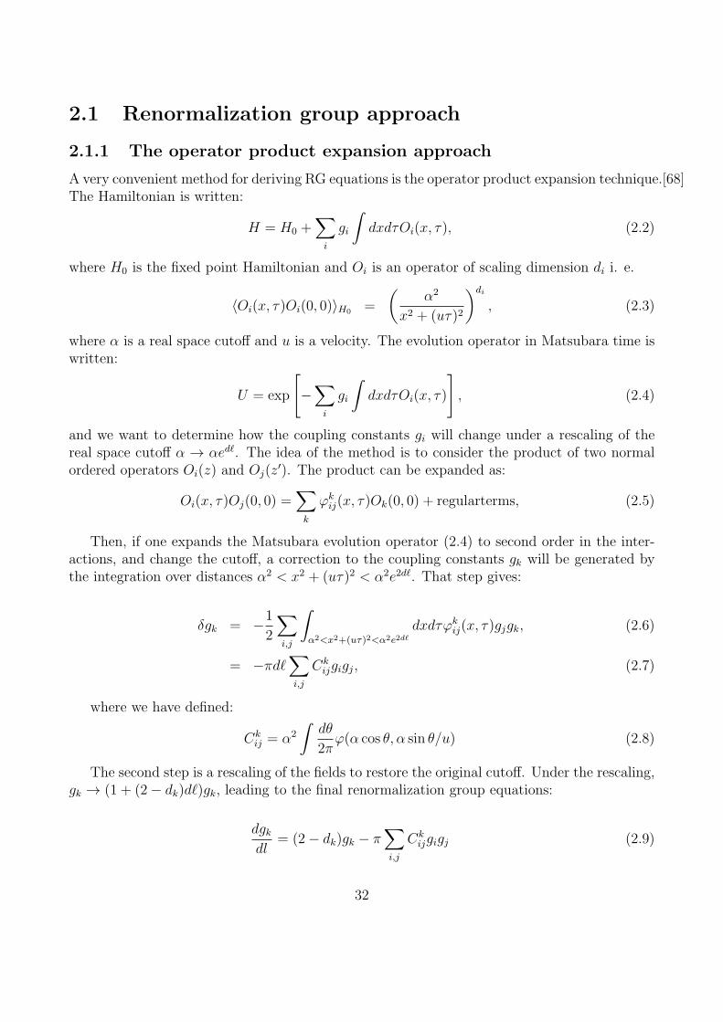
Figure 2.1: The renormalization group flow of the sine Gordon model. A stable fixed line existsfor K > 1.
2.1.2 Renormalization group for the sine Gordon model
The operator product expansion of the operators:
cos βφ(x, τ) cos βφ(0) =
(
α2
x2 + (uτ)2
)β2K/4 [
1− β2
2(x∂xφ+ τ∂τφ)
2 + . . .
]
+ . . . (2.10)
leads to the Kosterlitz-Thouless renormalization group equations:
dK
dℓ= −K
2
2
( g
πu
)2
(2.11)
dg
dℓ= 2(1−K)g (2.12)
It is convenient to introduce the dimensionless variable y(ℓ) = g(ℓ)/(πu). Because the flow issymmetric under y → −y and K → K, it is sufficient to discuss the case of y > 0. The flowdiagram is represented on the Figure. 2.1.
When K > 1, the cosine operator is irrelevant and the Luttinger liquid fixed point is stable.When K < 1 the cosine is relevant, the system flows to a strong coupling fixed point. At thestrong coupling fixed point, it is legitimate to expand the cosine around φ = 0, yielding a massterm ∝ φ2 which shows that the spectrum is fully gapped. For K far from 1, the RG flow isnearly vertical, and the gap behaves as ∆ ∼ u/α(g/u)1/(2−2K).
At the transition between the gapful and the gapless regime, there is a marginal flow, withthe cosine being marginally irrelevant. On that line, K(ℓ) = 1 + y(ℓ)/2 and the RG equationsreduce to a single equation:
dy
dℓ= −y(ℓ)2, (2.13)
with solution:
y(ℓ) =y(0)
1 + y(0)ℓ, (2.14)
33
with y(ℓ) → 0 for ℓ → ∞. Such marginal flow gives rise to logarithmic correlations to thecorrelation functions[41, 69]. One has in particular:
〈ei√2θ(x,τ)e−i
√2θ(0,0)〉 =
α
r[ln(r/α)1/2], (2.15)
〈cos√2φ(x, τ) cos
√2φ(0, 0)〉 =
α
r[ln(r/α)1/2], (2.16)
〈sin√2φ(x, τ) sin
√2φ(0, 0)〉 =
α
r[ln(r/α)−3/2], (2.17)
so that fluctuations towards antiferromagnetic ordering are enhanced over the fluctuations to-wards dimer order in the spin-1/2 chain at the isotropic point. In the Hubbard model withrepulsive interaction, this implies that spin density wave order dominates over charge densitywave order. The logarithmic corrections also affect macroscopic observables such as the mag-netic susceptibility. In, particular, in the spin-1/2 chain, with finite temperature, the RG flowhas to stop when the running cutoff αel
∗is of the order of the thermal length u/T giving at
finite temperature
K(T ) = 1 +1
2
y(0)
1 + y(0) ln(uα/T )≃ 1 +
1
2 ln(T0/T ), (2.18)
giving a susceptibility varying as[70]
χ(T ) =1
π2J
[
1 +1
2 ln(T0/T )
]
(2.19)
A similar logarithmic dependence of the magnetic susceptibility on the magnetic field can bededuced from Eq.(2.14). There exists also a line of marginally relevant flow with K = 1− y/2.Such a case is realized with the spin sector of the Hubbard model when U < 0, or the chargesector of the half-filled Hubbard model when U > 0 or with the frustrated antiferromagneticspin-1/2 chain with nearest neighbor exchange J1 and next-nearest neighbor exchange J2 >0.24J1. This time, the coupling constant is diverging at a scale ℓ∗ = −1/y(0). The excitationsof the sine-Gordon model are gapped.[66] and its spectrum is formed of massive solitons. Inthe J1 − J2 chain or the spin sector of the Hubbard model with U < 0, the massive solitons arespin-1/2 spinons. Since the total spin can only change by 1, these spinons are always formedor annihilated in pairs, giving a simple example of fractionnalized excitations.
2.2 The Luther-Emery point and the Ising model
2.2.1 Fermionization of the sine-Gordon model at the Luther-Emery
point
An interesting special point of the sine Gordon model is the Luther-Emery point[71] obtainedfor K = 1/2. At that point, the sine-Gordon model is a bosonized representation of a model
34
of free gapful fermions. Indeed, under the rescaling φ = φ/√2 and Π =
√2Π, the sine Gordon
Hamiltonian becomes:
H =
∫
dx
2πu[
(πΠ)2 + (∂xφ)2]
+2g
(2πα)2cos 2φ, (2.20)
Undoing the bosonization transformation by introducing the free fermions ψr = ei(θ−rφ)√2πα
yieldsthe Hamiltonian:
H =
∫
dx
[
−iu∑
r
rψ†r∂xψr +
g
πα
∑
r
ψ†rψ−r
]
, (2.21)
with gapful spectrum E(k) = ±√
(uk)2 + [g/(πα)]2.
2.2.2 The double Ising model and Dirac fermions in two dimensions
A mapping from the gapful free fermion model to a doubled Ising chain can be derived.[72, 73]For a single Ising chain,
H = −J∑
j
σxj σ
xj+1 − h
∑
j
σzj , (2.22)
there is a phase transition between a ferromagnetic phase with 〈σxj 〉 = ±σ0 6= 0 at small h
and a paramagnetic phase 〈σxj 〉 = 0 at large h. The Ising chain is known to possess a duality
transformation:
µzj = 2σx
j σxj+1, (2.23)
σzj = 2µx
jµxj+1, (2.24)
which exchanges J and 2h. For J = 2h the model is self-dual, indicating the transition point.The Jordan-Wigner transformation (1.57) allows to rewrite the Hamiltonian in terms of pseud-ofermions1:
H = −J4
∑
j
(c†j − cj)(c†j+1 + cj+1)− h
∑
j
(c†jcj − 1/2), (2.25)
It is convenient to introduce the Majorana fermions operators:
ζj =c†j − cj
i√2, (2.26)
ηj =c†j + cj√
2, (2.27)
1We don’t include the (−)n factor in that case.
35
that satisfy ζj = ζ†j , η=η†j and the anticommutation relations ζj, ζk = δjk and ηj, ηk = δjk
to rewrite:
H = −iJ2
∑
j
ζjηj+1 − ih∑
j
ζjηj. (2.28)
In terms of the Majorana fermion operators,
σxj =
ηj√2
∏
k<j
(2iηjζk) (2.29)
σzj = iζjηj, (2.30)
µzj = iζjηj+1, (2.31)
µxj =
∏
k<j
(2iηjζk) (2.32)
After a rotation in Majorana fermion space,
ζj =1√2(ψR,j − ψL,j), (2.33)
ηj =1√2(ψR,j + ψL,j), (2.34)
The Ising Hamiltonian is finally rewritten as:
H = − iJ4
∑
j
(ψR,jψR,j+1 − ψL,jψL,j+1) +∑
n
(
iJ
2ψR,j+1ψL,j+1 − ihψR,jψL,j
)
, (2.35)
Taking the continuum limit, the Hamiltonian becomes:
H = − iJ4
∑
j
(ψR(x)∂xψR(x)− ψL(x)∂xψL(x)) + i(J/2− h)
∫
dxψR(x)ψL(x), (2.36)
indicating that the Ising transition is obtained when the Majorana fermions become massless.If we now consider two Ising chains,
H = H1 +H2 (2.37)
Hn = −J∑
j
σxj,nσ
xj+1,n − h
∑
j
σzj,n, (2.38)
We can apply the previous mapping to each chain and derive a continuum representation ofthe form (2.36):
H =∑
n=1,2
[
− iJ4
∑
j,n
(ψ(n)R (x)∂xψ
(n)R (x)− ψ
(n)L (x)∂xψ
(n)L (x)) + i(J/2− h)
∫
dxψ(n)R (x)ψ
(n)L (x)
]
,(2.39)
36
which can be rewritten into a single Dirac fermion representation by introducing:
ΨR/L =1√2(ψ
(1)R/L + iψ
(1)R/L), (2.40)
so that:
H = −iv∫
dx(Ψ†R∂xΨR −Ψ†
L∂xΨL) + im
∫
dx(Ψ†RΨL −Ψ†
LΨR). (2.41)
If we now turn to the disorder operators, we have that:
2µxj,n =
∏
k<j
(2iζkηk) =∏
k<j
(2iψ(n)R,jψ
(n)L,k), (2.42)
So:
4µxj,1µ
xj,2 =
∏
k<j
∏
n=1,2
(2iψ(n)R,jψ
(n)L,k), (2.43)
=∏
k<j
(2Ψ†R,jΨR,j − 1)(2Ψ†
L,jΨL,j − 1) (2.44)
=∏
k<j
eiπ(Ψ†R,j
ΨR,j+Ψ†L,j
ΨL,j) (2.45)
= cos
[
π∑
k<j
(Ψ†R,jΨR,j +Ψ†
L,jΨL,j)
]
. (2.46)
We also have:
4σxj,1µ
xj,2 = (ψ
(1)R + ψ
(1)L ) cos
[
π∑
k<j
(Ψ†R,jΨR,j +Ψ†
L,jΨL,j)
]
, (2.47)
4µxj,1σ
xj,2 = (ψ
(2)R + ψ
(2)L ) cos
[
π∑
k<j
(Ψ†R,jΨR,j +Ψ†
L,jΨL,j)
]
, (2.48)
and:
4σxj,1σ
xj,2 = (ψ
(1)R + ψ
(1)L )(ψ
(2)R + ψ
(2)L ) cos
[
π∑
k<j
(Ψ†R,jΨR,j +Ψ†
L,jΨL,j)
]
, (2.49)
Applying bosonization, we obtain the relations:
µx1(x)µ
x2(x) = cosφ(x) (2.50)
σx1 (x)µ
x2(x) = cos θ(x) (2.51)
µx1(x)σ
x2 (x) = sin θ(x) (2.52)
σx1 (x)σ
x2 (x) = sinφ(x) (2.53)
The correlation functions of the two-dimensional Ising model in the vicinity of the critical pointare known[74] to be expressible in terms of Painleve III functions[75]. This allows us to obtainthe correlation functions of the sine-Gordon fields at the Luther-Emery point. We see that theoperators eiθ always have short range order, while the operators eiφ present a long range order.
37
2.3 Integrability of the sine-Gordon model and the Form-
factor approach
The integrability of the classical sine-Gordon model persists at the quantum level. Indeed,the quantum sine-Gordon model can be mapped in all generality to the massive Thirringmodel which is known from the work of Bergknoff and Thacker to be integrable by the BetheAnsatz[76, 77].
The excited states of the quantum sine-Gordon model can be described in terms of solitonsof mass uM/α, antisolitons of mass uM/α and (possibly) breathers. The dimensionless massM depends on g/u as[78] as:
M =2Γ(
K2−2K
)
Γ(1/2)Γ(
12−2K
)
[
Γ(1−K)
Γ(K)
g
4πu
] 12−2K
. (2.54)
The ground state expectation value of the exponential fields is conjectured to be[79]:
〈ein√2φ〉 =
[
πΓ(1−K)
Γ(K)
g
4π2u
] n2K(4−4K)
exp
∫ ∞
0
dt
t
[
sinh2(nKt)
2 sinh(Kt) sinh t cosh(1−K)t− n2K
2e−2t
]
,
(2.55)
with n < 1/K. However, in contrast to the classical sine-Gordon model, the breather massesuMn/α are quantized and satisfy the condition:
Mn = 2M sin
(
nπ
2
K
1−K
)
(2.56)
with n an integer, taking values from 1 to the integer part of 1/K−1. The condition (2.56) canbe derived from a semiclassical analysis[80]. According to (2.56), the breathers exist only forK < 1/2 i. e. only below the Luther-Emery point. The interpretation of this result is that forK < 1/2 the interaction between the Luther-Emery fermions is repulsive. As a result, a boundstate can be formed between a Luther-Emery hole (antisoliton) and a Luther-Emery fermion(soliton). For K > 1/2, the Luther-Emery fermion and the Luther-Emery hole repel each otherand no bound state can form.
In the case of the Hubbard model for U < 0 and |U | ≪ t, or the frustrated spin-1/2 chain,K < 1 and we have only massive spin-1/2 solitons. In the case of the dimerized spin-1/2 chain,K = 1/4, so that two breathers of masses M1 = 2M sin(π/6) = M and M2 = 2M sin(π/3) =M
√3 are present. The light breather of mass M and spin Sz = 0 forms a triplet with the
the soliton of spin Sz = 1 and the antisoliton of spin Sz = −1. The heavy breather of massM2 =M
√3 is a singlet excitation.[66, 81, 82]
2.3.1 S-matrix
The integrability of the quantum sine-Gordon model can be used to derive the exact free energy,but also to obtain the correlation functions using the Form factor expansion. To do that, it
38
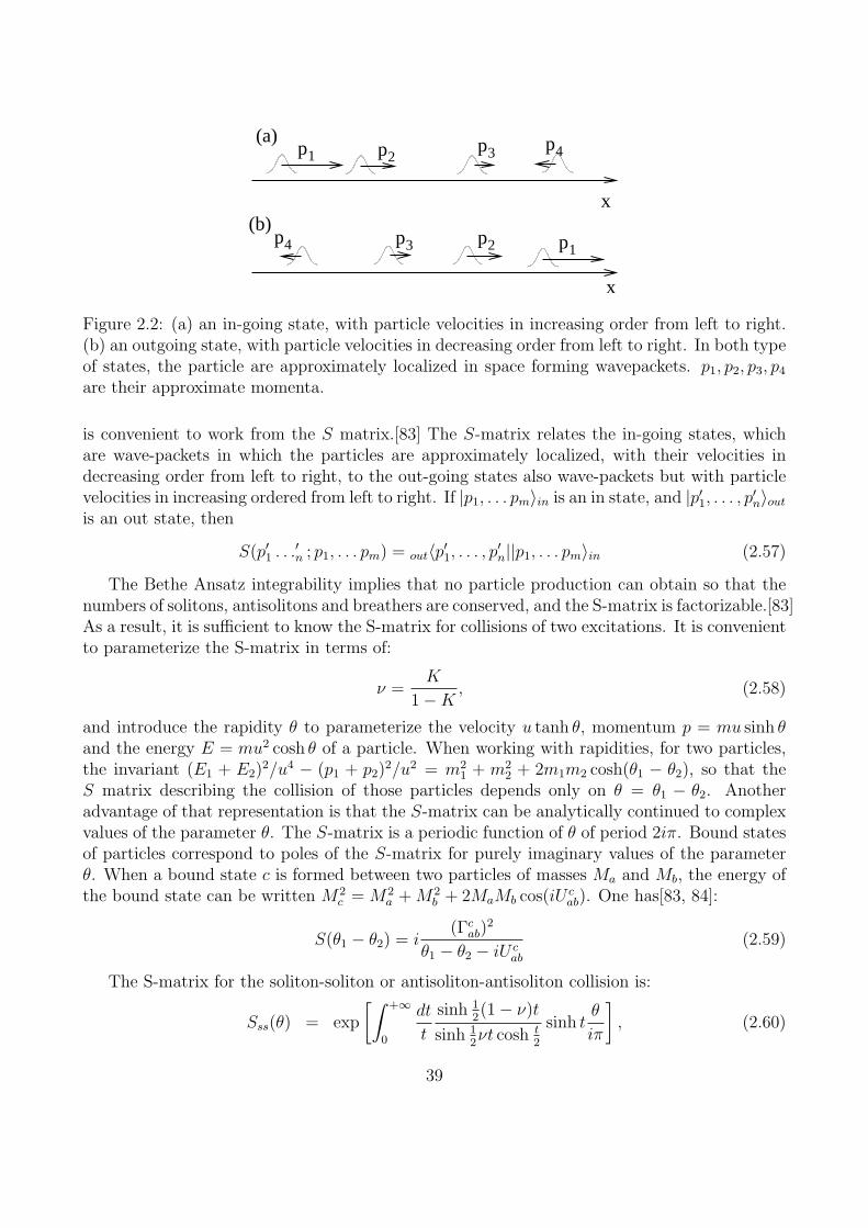
p1
p1
p2
p2
p3
p3
p4
p4
x
x
(a)
(b)
Figure 2.2: (a) an in-going state, with particle velocities in increasing order from left to right.(b) an outgoing state, with particle velocities in decreasing order from left to right. In both typeof states, the particle are approximately localized in space forming wavepackets. p1, p2, p3, p4are their approximate momenta.
is convenient to work from the S matrix.[83] The S-matrix relates the in-going states, whichare wave-packets in which the particles are approximately localized, with their velocities indecreasing order from left to right, to the out-going states also wave-packets but with particlevelocities in increasing ordered from left to right. If |p1, . . . pm〉in is an in state, and |p′1, . . . , p′n〉outis an out state, then
S(p′1 . . .′n ; p1, . . . pm) = out〈p′1, . . . , p′n||p1, . . . pm〉in (2.57)
The Bethe Ansatz integrability implies that no particle production can obtain so that thenumbers of solitons, antisolitons and breathers are conserved, and the S-matrix is factorizable.[83]As a result, it is sufficient to know the S-matrix for collisions of two excitations. It is convenientto parameterize the S-matrix in terms of:
ν =K
1−K, (2.58)
and introduce the rapidity θ to parameterize the velocity u tanh θ, momentum p = mu sinh θand the energy E = mu2 cosh θ of a particle. When working with rapidities, for two particles,the invariant (E1 + E2)
2/u4 − (p1 + p2)2/u2 = m2
1 + m22 + 2m1m2 cosh(θ1 − θ2), so that the
S matrix describing the collision of those particles depends only on θ = θ1 − θ2. Anotheradvantage of that representation is that the S-matrix can be analytically continued to complexvalues of the parameter θ. The S-matrix is a periodic function of θ of period 2iπ. Bound statesof particles correspond to poles of the S-matrix for purely imaginary values of the parameterθ. When a bound state c is formed between two particles of masses Ma and Mb, the energy ofthe bound state can be written M2
c =M2a +M2
b + 2MaMb cos(iUcab). One has[83, 84]:
S(θ1 − θ2) = i(Γc
ab)2
θ1 − θ2 − iU cab
(2.59)
The S-matrix for the soliton-soliton or antisoliton-antisoliton collision is:
Sss(θ) = exp
[∫ +∞
0
dt
t
sinh 12(1− ν)t
sinh 12νt cosh t
2
sinh tθ
iπ
]
, (2.60)
39
The S-matrix describing a collision between soliton and antisoliton without momentumexchange is:
S(t)ss (θ) =
sinh θ/ν
sinh(iπ − θ)/νSss(θ), (2.61)
while the S-matrix describing a collision between soliton and antisoliton with momentumexchange is:
S(r)ss (θ) =
sinh iπ/ν
sinh(iπ − θ)/νSss(θ), (2.62)
We notice that when 1/ν is integer, the matrix describing reflection vanishes. The pointsare called reflectionless points.
When breathers exist, we also have soliton-breather:
Ssbk(θ) = (−)k exp
[∫ +∞
0
dt
t
2 cosh ν2t sinh ν
2kt
sinh 12νt cosh t
2
sinh tθ
iπ
]
, (2.63)
and breather-breather (k < l):
Sbkbl(θ) = (−)k exp
[∫ +∞
0
dt
t
4 cosh ν2t sinh ν
2kt cosh 1
2(1− νl)t
sinh 12νt cosh t
2
sinh tθ
iπ
]
, (2.64)
Sbkbk(θ) = (−)k exp
[∫ +∞
0
dt
t2cosh ν
2t sinh 1
2(2kν − 1)t+ sinh 1
2(1− ν)t
sinh 12νt cosh t
2
sinh tθ
iπ
]
. (2.65)
2.3.2 Bethe Ansatz at the reflectionless points
At the reflectionless points, there is no backscattering of solitons, antisolitons or breathers andthe S-matrix is simply describing a phase-shift of the particles after a collision. Such situationmakes the description of the conditions to be satisfied by the rapidities of the particles whenperiodic boundary conditions are imposed particularly simple to write.[85] Indeed, if we considera particle of rapidity θj and mass mj going from position x to position x+L ≡ x it will receive aphase-shift eimj sinh θjL resulting from its momentum, and another phase-shift
∏
j 6=k Sjk(θk − θj)from the collisions with the other particles. These phase shifts have to compensate each otherso that the periodic boundary conditions are satisfied and:
eimj sinh θjL∏
k 6=j
Sjk(θj − θk) = 1. (2.66)
Taking the logarithm of (2.66), we find:
mjL sinh θj +1
i
∑
j 6=k
lnSjk(θk − θj) = 2πIj, (2.67)
40
where the Ij’s are integer. Introducing the densities of solitons, antisolitons and breathers, theequations (2.67) can be rewritten as integral equations[85]:
Mα cosh θ +∑
β
∫ ∞
−∞Kαβ(θ − θ′)ρβ(θ
′) = 2π[ρβ(θ) + ρhβ(θ′)], (2.68)
where α = s, s, bj indicates whether ρα(θ) is a density of solitons (s), antisolitons (s) or breathers(bj), ρ
hβ(θ) being a density of unoccupied soliton, antisoliton or breather states. We have also
defined:
Kαβ(θ) =1
i
d
dθlnSαβ(θ). (2.69)
The dimensionless free energy F = (α2/u)F is obtained from the method of Yang and Yang.[86,87, 88] The total energy of an excited state is given by:
E = EGS +
∫
dθ∑
α
Mα cosh θρα(θ), (2.70)
with the dimensionless ground state energy density EGS given by:
EGS = −M2
4tan
(
πK
2− 2K
)
(2.71)
while the entropy is given by:
S =∑
α
∫
dθ[(ρα + ρhα)(θ) ln(ρα + ρhα)(θ)− ρα(θ) ln ρα(θ)− ρhα(θ) ln ρhα(θ)]. (2.72)
We have to minimize the free energy F = E−TS with respect to the densities ρ and ρh subjectto the condition (2.68). Introducing the pseudoenergies:
ρα(θ)
ρhα(θ)= e−ǫα(θ)/T , (2.73)
we find:
0 = δF =∑
α
[
mα cosh θ − T ln(1 + eǫα(θ)/T )]
δρα − T ln(1 + e−ǫα(θ)/T )δρhα (2.74)
δρhα = −δρα +1
2π
∑
β
∫
dθ′Kαβ(θ − θ′)δρβ(θ′) (2.75)
substituting the second line into the first equation, we obtain:
mα cosh θ = ǫα(θ)−T
2π
∫
dθ′∑
β
Kαβ(θ − θ′) ln(1 + e−ǫβ(θ′)/T ). (2.76)
41
The non-linear integral equations (2.76) must be solved in order to obtain the pseudoenergies.Once the pseudoenergies are known, it is possible to express the free energy using:
F = EGS +
∫
dθ
[
∑
α
∫
dθmα cosh θ − ǫα(θ)ρα(θ)− T (ρα + ρhα) ln(1 + e−ǫα/T )
]
(2.77)
= EGS − T
2π
∫
dθ∑
α
mα cosh θ ln(1 + e−ǫα/T ), (2.78)
where, to obtain the last line we have used the integral equations (2.76) and the condition (2.68).
2.3.3 The form factor expansion
The form factor expansion allows the calculation of correlation functions in integrable models.It has been applied to the calculation of conductivity in one-dimensional Mott insulators[89, 90,91], spin-spin correlation functions in gapful spin chains [92, 93, 94, 95] and spectral functionsin metals with spin gap[96]. In the present section, we will first describe the principle of theForm factor expansion, and we will then describe the calculation of the simplest form factors.
Principle of the method
For any translationally invariant system, the Matsubara correlation functions in the groundstate can be written as:
〈A(x, τ)A(0, 0)〉 =∑
n
〈0|e−iPx+τHAeiPx−τH |n >< n|A|0 > (2.79)
=∑
n
| < n|A|0 > |2eiPnx−Enτ , (2.80)
where |n > is a simultaneous eigenstate of the energy operator H|n >= En|n > and of themomentum operator P |n >= Pn|n >. In a general model, the computation of all eigenval-ues and eigenstates is a daunting task. However, in the case of an integrable model such asthe sine-Gordon model, the problem is simpler. First, the eigenstates are simply describedin terms of the rapidities of the solitons, antisolitons and breathers, and the eigenvalues aresimply Pn =
∑
j mj sinh θj and En =∑
j mj cosh θj. Second, it is possible to obtain equationsrelating the matrix elements FA(θ1, . . . , θn) = 〈θ1, . . . , θn|A|0〉 (these matrix elements are calledform factors) to the S-matrix.[97] Solving these equations allows to write a series expansion ofEq. (2.79) the terms of which are indexed by the number of solitons, antisolitons and breathersin the expansion. Finally, for gapped models such as the sine-Gordon model, the term e−Enτ
decays exponentially with τ over a scale inversely proportional to the sum of the masses ofthe breathers, solitons and antisolitons appearing in the eigenstate |n >. As a result, the firstterms of the series already give an accurate approximation of the Matsubara correlation func-tion (2.79). If we were considering the imaginary part of a response function, the situationwould be even better. Indeed, the expression of the response function being:
IA(q, ω) =∑
n
| < n|A|0 > |2δ(q − Pn)δ(ω − En), (2.81)
42
for ω < En, the contribution of the eigenstate |n > to the response function is exactly zero. Sofor fixed ω and with a gapful model, only the terms with a total mass of the excitations lessthan ω need to be summed in (2.81) to obtain the exact answer.
The equations defining the form factors
For the n-particle form factor, we define[97]:
〉0|A(x)|〈θ1, . . . θn〉in = eix(m1 sinh θ1+...+sinh θn)F(n)A (θ1, . . . θn) (2.82)
As a result of the Lorentz-like invariance of the sine-Gordon model, FA(θj) depends only onthe differences θj − θk. The form factor possesses invariance under the combination of chargeconjugation, parity and time reversal, so that:
〉0|A(x)|〈θ1, . . . , θn〉out = F(n)A (−θ1, . . . ,−θn) (2.83)
It also possesses the crossing symmetry, such that:
out〈θ1, . . . , θm|A(x)|〈θm+1, . . . , θn〉in = F(n)A (2.84)
If we consider the two-particle form-factor and insert a resolution of the identity in Eq. (2.82)using the out-going state as a basis, we find with (2.83) that:
F(2)A (θ2 − θ1) = S(θ1 − θ2)FA(θ1 − θ2) (2.85)
and from (2.84):
FA(iπ − θ) = FA(iπ + θ) (2.86)
The equation (2.85) is called Watson’s equation. It allows to find the two-particle form factorby solving a Riemann-Hilbert problem.[98] When the S matrix can be written as:
S(θ) = exp
[∫ +∞
0
dtf(t) sinhtθ
iπ
]
, (2.87)
The minimal solution of the Riemann Hilbert problem is given by[97, 99]:
Fmin.(θ) = exp
[∫ +∞
0
dtf(t)sin2[t(iπ − θ)/2π]
sinh t
]
(2.88)
The solution (2.88) is free from poles. The general solution is of the form:
F (θ) = K(θ)Fmin.(θ), (2.89)
where K(θ) = K(−θ) = K(θ + 2iπ). The factor K(θ) contains all the poles of the physicalform factor.
43
In the case of the general multi-particle form-factors, the set of equations to be solved isdiscussed in[84, 100, 99]. This set of equation is:
FA(θ1, . . . θj, θj+1, . . . , θn) = S(θj − θj + 1)FA(θ1, . . . θj+1, θj , . . . , θn) (2.90)
FA(2iπ + θ1, θ2, . . . , θn) = FA(θ2, . . . , θn, θ1) (2.91)
To these equations, conditions fixing the position of the poles must be added. The first oneis related to kinematic poles:
−i limθ→θ′
(θ − θ′)FA(θ′ + iπ, θ, θ1, . . . , θn) =
(
1−n∏
l=1
S(θ − θl)
)
FA(θ1, . . . θn),
(2.92)
where θ and θ′ are the rapidities of a soliton and and an antisoliton. These poles correspondthe annihilation of a particle and an antiparticle, the total energy being 4M2 cosh(iπ/2)2 = 0when θ−θ′ = iπ. These poles relate the n+2 particle form factor to the n particle form factor.The other one is related to bound state poles. When a bound state exists, one has the relation(with the same notations as in (2.59):
−i limθ−θ′→iUc
ab
F (θ, θ′, θ1, . . . , θn) = ΓcabF
(
θ + θ′
2, θ1, . . . , θn
)
, (2.93)
which relates the n + 1 particles form factor to the n-particles form factor (the first particlebeing a bound state).
44
Chapter 3
A brief review of experimental systems
3.1 Quasi-one dimensional conductors
These systems are three-dimensional solids with a highly anisotropic structure that can beviewed as an an array of weakly coupled one-dimensional chains. As a result, they can beexpected to show some Tomonaga-Luttinger liquid features. However, in all those quasi-onedimensional conductors, interchain couplings are relevant perturbations that destabilize theLuttinger liquid fixed point[101]. If we call t⊥ the interchain hopping, a renormalization groupargument shows that, when t⊥ is relevant, below a temperature:
TX ∝ TF
(
t⊥EF
)
4Kρ
6Kρ−K2ρ−1
, (3.1)
the one-dimensional chains cannot be considered decoupled and a Fermi liquid is restored.[101]One may hope that since t⊥ is irrelevant for eitherKρ < 3−2
√2 orKρ > 3+2
√2 the Tomonaga-
Luttinger liquid could be stable for large interactions. However, interchain exchange couplingand interchain Josephson coupling are also present[102, 103, 104] and become relevant forrespectivelyKρ < 1 andKρ > 1 giving rise respectively to antiferromagnetic or superconductinglong range order. As a result, the hints of Tomonaga-Luttinger liquid physics can only beobserved in a regime of sufficiently large temperature or high frequency. With these limitationsin mind, we discuss some of the hints of Tomonaga-Luttinger liquid properties in these materials.
3.1.1 TTF-TCNQ
The organic conductor TTF-TCNQ (tetrathiafulvalenium-tetracyanoquinodimethane) is madeof chains of stacked organic molecules TTF and TCNQ. The structure is monoclinic, with spacegroup P21/c, and lattice parameters a = 12, 298 A, b = 3, 819 A, c = 18, 468 Aet β = 104, 46o.The electronic orbitals overlap most strongly along the b axis, and more weakly along the otherdirections. TCNQ is an electron acceptor molecule, while TTF is an electron donor molecule,and as a result of electron transfer, the TTF chains are hole doped (nh = 1.41)while the TCNQchains are electron doped (ne = 0.59). A Peierls instability exists for T < 54K. It is know
45
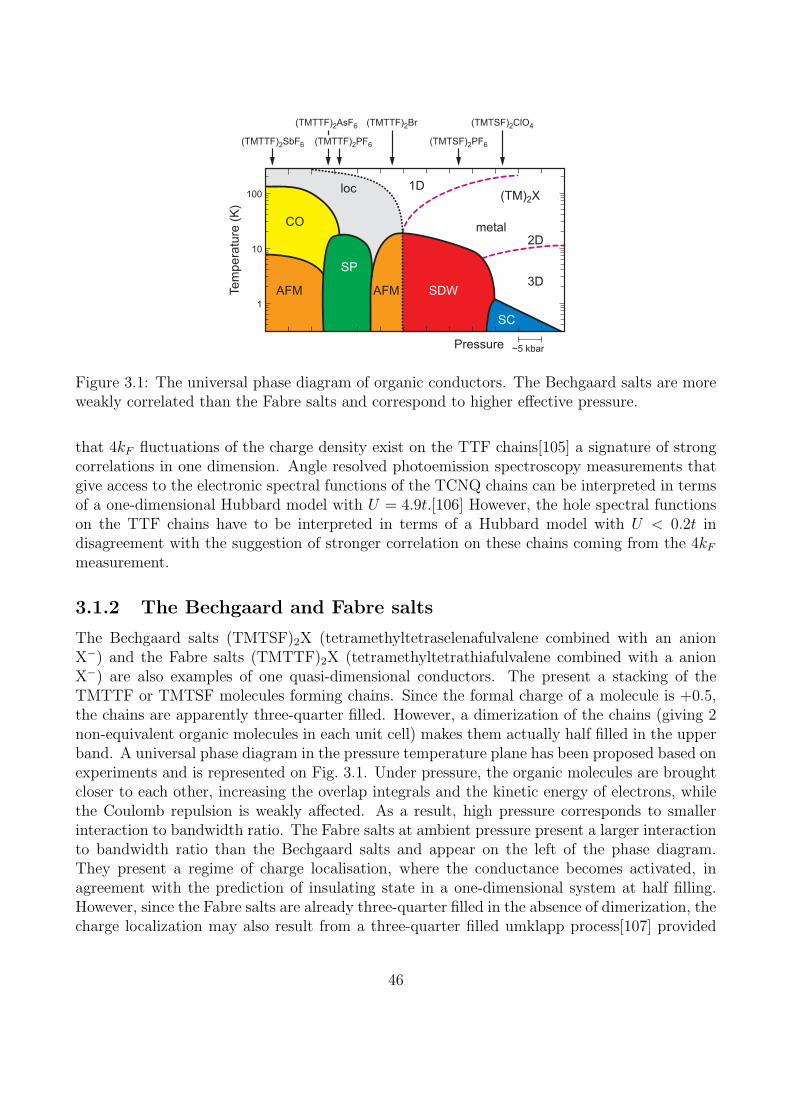
10
100
1
(TMTSF)2PF6
(TMTTF)2Br(TMTTF)2AsF6 (TMTSF)2ClO4
Pressure
SP
loc
CO
SC
AFMAFM SDW
metal
~5 kbar
Te
mp
era
ture
(K
)
(TM)2X1D
2D
3D
(TMTTF)2PF6(TMTTF)2SbF6
Figure 3.1: The universal phase diagram of organic conductors. The Bechgaard salts are moreweakly correlated than the Fabre salts and correspond to higher effective pressure.
that 4kF fluctuations of the charge density exist on the TTF chains[105] a signature of strongcorrelations in one dimension. Angle resolved photoemission spectroscopy measurements thatgive access to the electronic spectral functions of the TCNQ chains can be interpreted in termsof a one-dimensional Hubbard model with U = 4.9t.[106] However, the hole spectral functionson the TTF chains have to be interpreted in terms of a Hubbard model with U < 0.2t indisagreement with the suggestion of stronger correlation on these chains coming from the 4kFmeasurement.
3.1.2 The Bechgaard and Fabre salts
The Bechgaard salts (TMTSF)2X (tetramethyltetraselenafulvalene combined with an anionX−) and the Fabre salts (TMTTF)2X (tetramethyltetrathiafulvalene combined with a anionX−) are also examples of one quasi-dimensional conductors. The present a stacking of theTMTTF or TMTSF molecules forming chains. Since the formal charge of a molecule is +0.5,the chains are apparently three-quarter filled. However, a dimerization of the chains (giving 2non-equivalent organic molecules in each unit cell) makes them actually half filled in the upperband. A universal phase diagram in the pressure temperature plane has been proposed based onexperiments and is represented on Fig. 3.1. Under pressure, the organic molecules are broughtcloser to each other, increasing the overlap integrals and the kinetic energy of electrons, whilethe Coulomb repulsion is weakly affected. As a result, high pressure corresponds to smallerinteraction to bandwidth ratio. The Fabre salts at ambient pressure present a larger interactionto bandwidth ratio than the Bechgaard salts and appear on the left of the phase diagram.They present a regime of charge localisation, where the conductance becomes activated, inagreement with the prediction of insulating state in a one-dimensional system at half filling.However, since the Fabre salts are already three-quarter filled in the absence of dimerization, thecharge localization may also result from a three-quarter filled umklapp process[107] provided
46
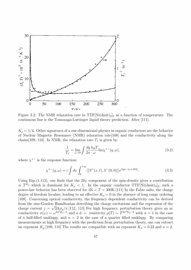
Figure 3.2: The NMR relaxation rate in TTF[Ni(dmit)2]2 as a function of temperature. Thecontinuous line is the Tomonaga-Luttinger liquid theory prediction. After [111].
Kρ < 1/4. Other signatures of a one-dimensional physics in organic conductors are the behaviorof Nuclear Magnetic Resonance (NMR) relaxation rate[108] and the conductivity along thechains[109, 110]. In NMR, the relaxation rate T1 is given by:
1
T1= lim
ω→0
∫
dq
2π
kBT
ωImχ+−(q, ω), (3.2)
where χ+− is the response function:
χ+−(q, ω) = i
∫
dx
∫ +∞
0
〈[S+(x, t), S−(0, 0)]〉ei[qx−(ω+i0)t]. (3.3)
Using Eqs.(1.112), one finds that the 2kF component of the spin-density gives a contribution∝ TKρ which is dominant for Kρ < 1. In the organic conductor TTF[Ni(dmit)2]2, such apower-law behavior has been observed for 1K < T < 300K.[111] In the Fabre salts, the chargedegree of freedom localize, leading to an effective Kρ = 0 in the absence of long range ordering[108]. Concerning optical conductivity, the frequency dependent conductivity can be derivedfrom the sine-Gordon Hamiltonian describing the charge excitations and the expression of thecharge current j =
√2∂tφρ/π.[112, 113] For high frequency, perturbation theory gives an ac
conductivity σ(ω) ∼ ω4n2Kρ−5 and a d. c. resistivity ρ(T ) ∼ T 4n2Kρ−3 with n = 1 in the caseof a half-filled umklapp, and n = 2 in the case of a quarter filled umklapp. By comparingmeasurements at high frequency with the prediction from perturbation theory, one can extractan exponent Kρ.[109, 110] The results are compatible with an exponent Kρ = 0.22 and n = 2.
47
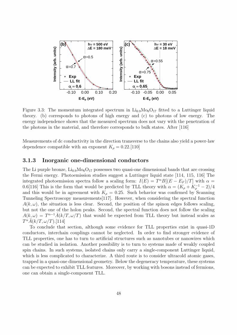
Inte
nsi
ty (
arb
. un
its)
0.200.100.00-0.10
E-EF (eV)
Exp LL fit !" 0.6
α=0.5
α=0.7
Inte
nsi
ty (
arb
. un
its)
-0.10 -0.05 0.00 0.05
E-EF (eV)
Exp LL fit !"!0.65
α=0.75
α=0.55
(b) h# = 500 eV h# = 30 eV (c)$E = 180 meV $E = 18 meV
#
$
Figure 3.3: The momentum integrated spectrum in Li0.9Mo6O17 fitted to a Luttinger liquidtheory. (b) corresponds to photons of high energy and (c) to photons of low energy. Theenergy independence shows that the measured spectrum does not vary with the penetration ofthe photons in the material, and therefore corresponds to bulk states. After [116]
Measurements of dc conductivity in the direction transverse to the chains also yield a power-lawdependence compatible with an exponent Kρ = 0.22.[110]
3.1.3 Inorganic one-dimensional conductors
The Li purple bronze, Li0.9Mo6O17 possesses two quasi-one dimensional bands that are crossingthe Fermi energy. Photoemission studies suggest a Luttinger liquid state [114, 115, 116] Theintegrated photoemission spectra follow a scaling form: I(E) = T αB[(E − EF )/T ] with α =0.6[116] This is the form that would be predicted by TLL theory with α = (Kρ +K−1
ρ − 2)/4and this would be in agreement with Kρ = 0.25. Such behavior was confirmed by ScanningTunneling Spectroscopy measurements[117]. However, when considering the spectral functionA(k, ω), the situation is less clear. Second, the position of the spinon edges follows scaling,but not the one of the holon peaks. Second, the spectral function does not follow the scalingA(k, ω) = T α−1A(k/T, ω/T ) that would be expected from TLL theory but instead scales asT αA(k/T, ω/T ).[114]
To conclude that section, although some evidence for TLL properties exist in quasi-1Dconductors, interchain couplings cannot be neglected. In order to find stronger evidence ofTLL properties, one has to turn to artificial structures such as nanotubes or nanowires whichcan be studied in isolation. Another possibility is to turn to systems made of weakly coupledspin chains. In such systems, isolated chains only carry a single-component Luttinger liquid,which is less complicated to characterize. A third route is to consider ultracold atomic gases,trapped in a quasi-one dimensional geometry. Below the degeneracy temperature, these systemscan be expected to exhibit TLL features. Moreover, by working with bosons instead of fermions,one can obtain a single-component TLL.
48
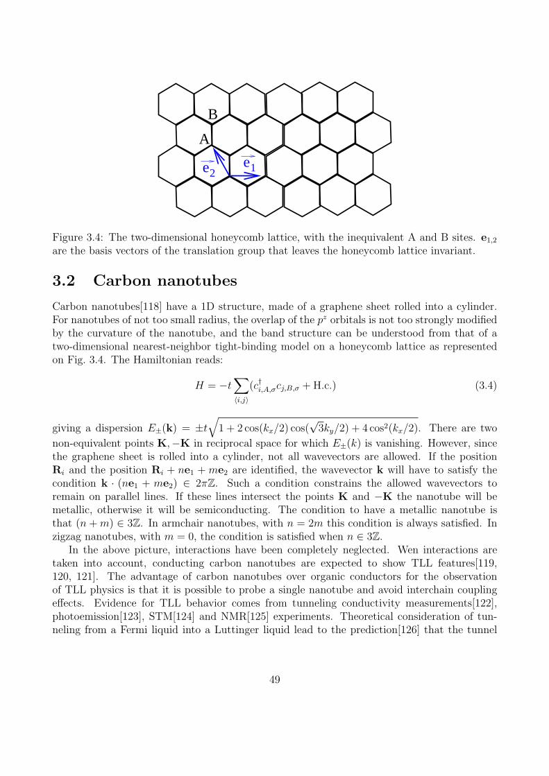
e1
A
B
e2
Figure 3.4: The two-dimensional honeycomb lattice, with the inequivalent A and B sites. e1,2are the basis vectors of the translation group that leaves the honeycomb lattice invariant.
3.2 Carbon nanotubes
Carbon nanotubes[118] have a 1D structure, made of a graphene sheet rolled into a cylinder.For nanotubes of not too small radius, the overlap of the pz orbitals is not too strongly modifiedby the curvature of the nanotube, and the band structure can be understood from that of atwo-dimensional nearest-neighbor tight-binding model on a honeycomb lattice as representedon Fig. 3.4. The Hamiltonian reads:
H = −t∑
〈i,j〉(c†i,A,σcj,B,σ +H.c.) (3.4)
giving a dispersion E±(k) = ±t√
1 + 2 cos(kx/2) cos(√3ky/2) + 4 cos2(kx/2). There are two
non-equivalent points K,−K in reciprocal space for which E±(k) is vanishing. However, sincethe graphene sheet is rolled into a cylinder, not all wavevectors are allowed. If the positionRi and the position Ri + ne1 + me2 are identified, the wavevector k will have to satisfy thecondition k · (ne1 + me2) ∈ 2πZ. Such a condition constrains the allowed wavevectors toremain on parallel lines. If these lines intersect the points K and −K the nanotube will bemetallic, otherwise it will be semiconducting. The condition to have a metallic nanotube isthat (n+m) ∈ 3Z. In armchair nanotubes, with n = 2m this condition is always satisfied. Inzigzag nanotubes, with m = 0, the condition is satisfied when n ∈ 3Z.
In the above picture, interactions have been completely neglected. Wen interactions aretaken into account, conducting carbon nanotubes are expected to show TLL features[119,120, 121]. The advantage of carbon nanotubes over organic conductors for the observationof TLL physics is that it is possible to probe a single nanotube and avoid interchain couplingeffects. Evidence for TLL behavior comes from tunneling conductivity measurements[122],photoemission[123], STM[124] and NMR[125] experiments. Theoretical consideration of tun-neling from a Fermi liquid into a Luttinger liquid lead to the prediction[126] that the tunnel
49
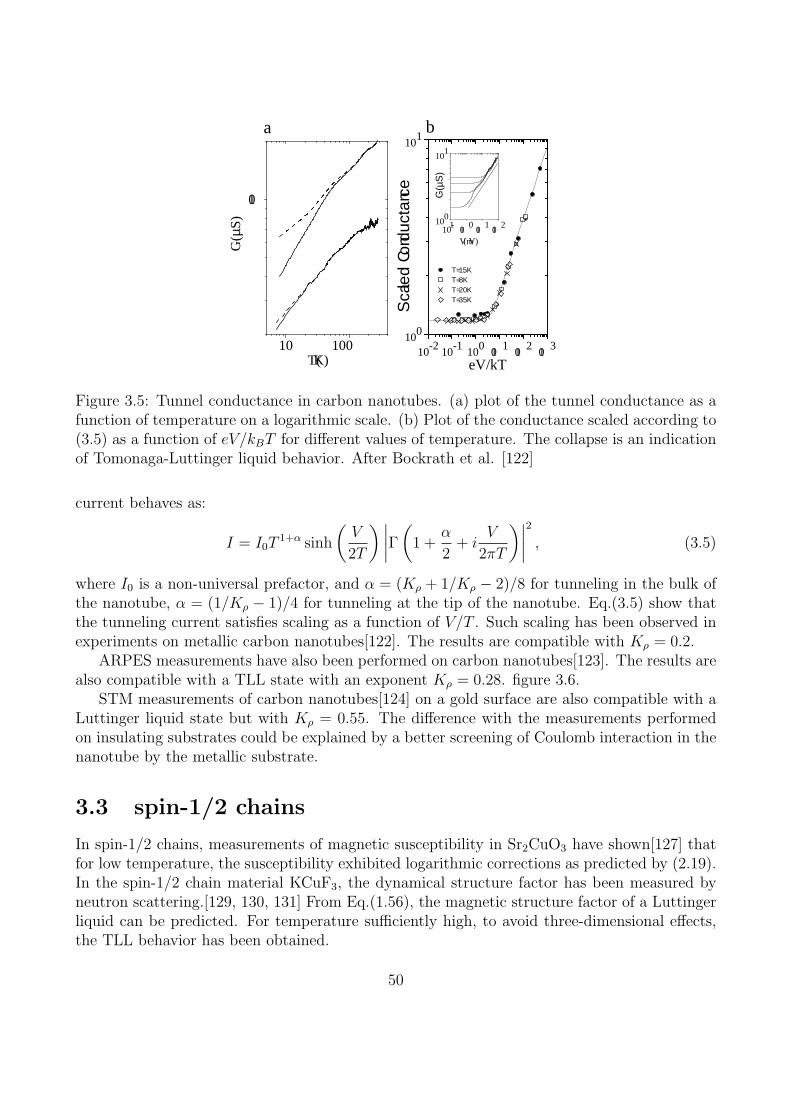
10 -2 10 -1 10 0 1 0 1 1 0 2 1 0 3 10 0
10 1
G( µ
S)
Sca
led
C on
duct
an ce
T= 1. 5 K T= 8 K T= 20 K T= 35 K
eV/kT
10 - 1
1 0 0
1 0 1
1 0 2 10
0
10 1
V (m V)
10 100
1 0
G( µ
S)
T( K)
a b
Figure 3.5: Tunnel conductance in carbon nanotubes. (a) plot of the tunnel conductance as afunction of temperature on a logarithmic scale. (b) Plot of the conductance scaled according to(3.5) as a function of eV/kBT for different values of temperature. The collapse is an indicationof Tomonaga-Luttinger liquid behavior. After Bockrath et al. [122]
current behaves as:
I = I0T1+α sinh
(
V
2T
) ∣
∣
∣
∣
Γ
(
1 +α
2+ i
V
2πT
)∣
∣
∣
∣
2
, (3.5)
where I0 is a non-universal prefactor, and α = (Kρ + 1/Kρ − 2)/8 for tunneling in the bulk ofthe nanotube, α = (1/Kρ − 1)/4 for tunneling at the tip of the nanotube. Eq.(3.5) show thatthe tunneling current satisfies scaling as a function of V/T . Such scaling has been observed inexperiments on metallic carbon nanotubes[122]. The results are compatible with Kρ = 0.2.
ARPES measurements have also been performed on carbon nanotubes[123]. The results arealso compatible with a TLL state with an exponent Kρ = 0.28. figure 3.6.
STM measurements of carbon nanotubes[124] on a gold surface are also compatible with aLuttinger liquid state but with Kρ = 0.55. The difference with the measurements performedon insulating substrates could be explained by a better screening of Coulomb interaction in thenanotube by the metallic substrate.
3.3 spin-1/2 chains
In spin-1/2 chains, measurements of magnetic susceptibility in Sr2CuO3 have shown[127] thatfor low temperature, the susceptibility exhibited logarithmic corrections as predicted by (2.19).In the spin-1/2 chain material KCuF3, the dynamical structure factor has been measured byneutron scattering.[129, 130, 131] From Eq.(1.56), the magnetic structure factor of a Luttingerliquid can be predicted. For temperature sufficiently high, to avoid three-dimensional effects,the TLL behavior has been obtained.
50
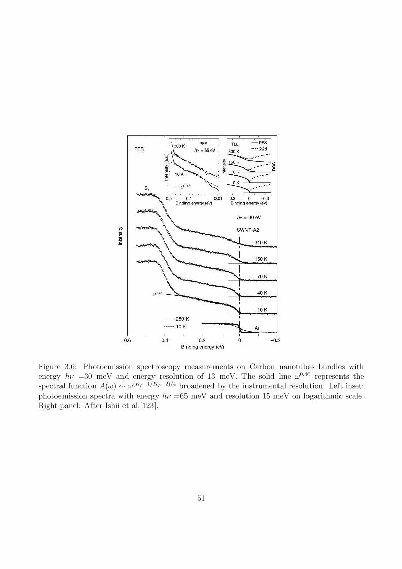
Figure 3.6: Photoemission spectroscopy measurements on Carbon nanotubes bundles withenergy hν =30 meV and energy resolution of 13 meV. The solid line ω0.46 represents thespectral function A(ω) ∼ ω(Kρ+1/Kρ−2)/4 broadened by the instrumental resolution. Left inset:photoemission spectra with energy hν =65 meV and resolution 15 meV on logarithmic scale.Right panel: After Ishii et al.[123].
51
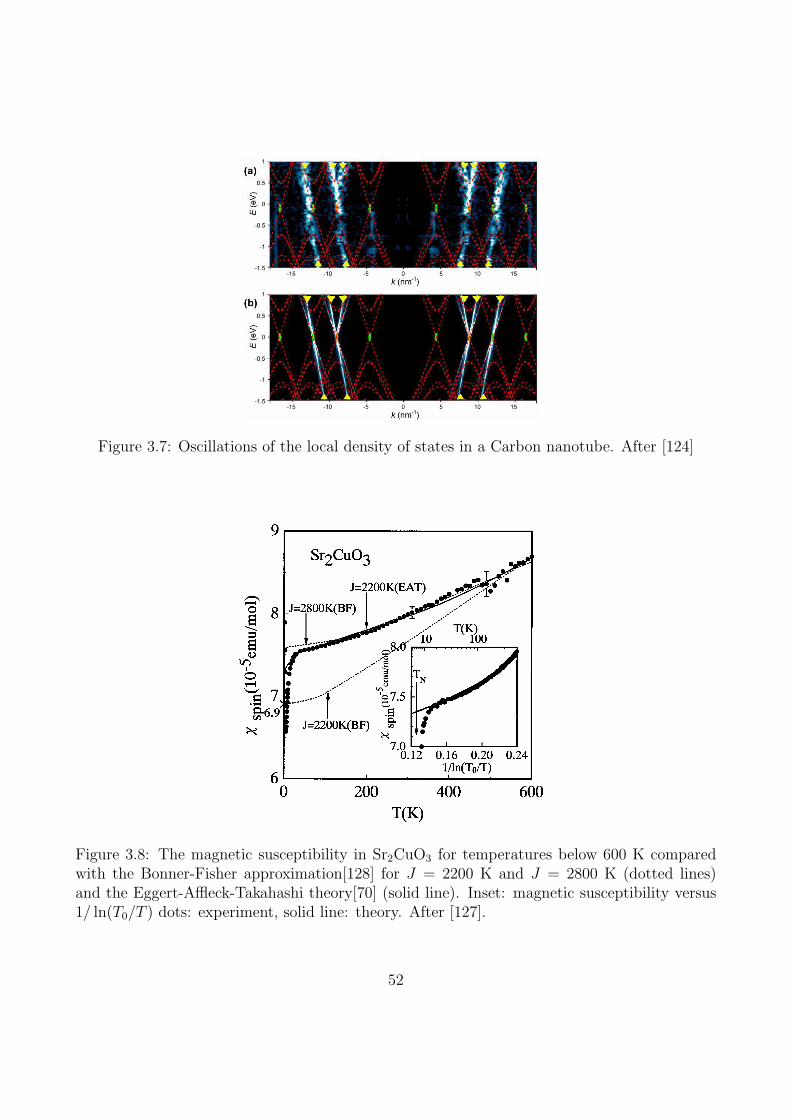
Figure 3.7: Oscillations of the local density of states in a Carbon nanotube. After [124]
Figure 3.8: The magnetic susceptibility in Sr2CuO3 for temperatures below 600 K comparedwith the Bonner-Fisher approximation[128] for J = 2200 K and J = 2800 K (dotted lines)and the Eggert-Affleck-Takahashi theory[70] (solid line). Inset: magnetic susceptibility versus1/ ln(T0/T ) dots: experiment, solid line: theory. After [127].
52
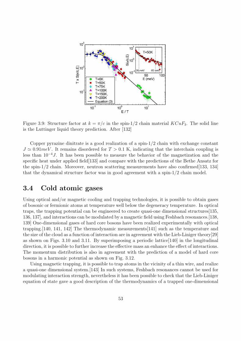
Figure 3.9: Structure factor at k = π/c in the spin-1/2 chain material KCuF3. The solid lineis the Luttinger liquid theory prediction. After [132]
Copper pyrazine dinitrate is a good realization of a spin-1/2 chain with exchange constantJ ≃ 0.91meV . It remains disordered for T > 0.1 K, indicating that the interchain coupling isless than 10−4J . It has been possible to measure the behavior of the magnetization and thespecific heat under applied field[133] and compare with the predictions of the Bethe Ansatz forthe spin-1/2 chain. Moreover, neutron scattering measurements have also confirmed[133, 134]that the dynamical structure factor was in good agreement with a spin-1/2 chain model.
3.4 Cold atomic gases
Using optical and/or magnetic cooling and trapping technologies, it is possible to obtain gasesof bosonic or fermionic atoms at temperature well below the degeneracy temperature. In opticaltraps, the trapping potential can be engineered to create quasi-one dimensional structures[135,136, 137], and interactions can be modulated by a magnetic field using Feshbach resonances.[138,139] One-dimensional gases of hard core bosons have been realized experimentally with opticaltrapping.[140, 141, 142] The thermodynamic measurements[141] such as the temperature andthe size of the cloud as a function of interaction are in agreement with the Lieb-Liniger theory[29]as shown on Figs. 3.10 and 3.11. By superimposing a periodic lattice[140] in the longitudinaldirection, it is possible to further increase the effective mass an enhance the effect of interactions.The momentum distribution is also in agreement with the prediction of a model of hard corebosons in a harmonic potential as shown on Fig. 3.12.
Using magnetic trapping, it is possible to trap atoms in the vicinity of a thin wire, and realizea quasi-one dimensional system.[143] In such systems, Feshbach resonances cannot be used formodulating interaction strength, nevertheless it has been possible to check that the Lieb-Linigerequation of state gave a good description of the thermodynamics of a trapped one-dimensional
53
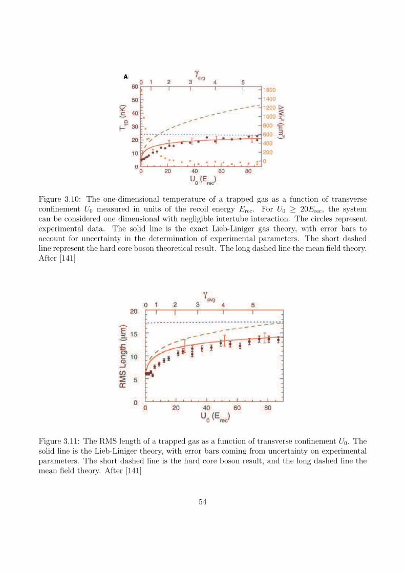
Figure 3.10: The one-dimensional temperature of a trapped gas as a function of transverseconfinement U0 measured in units of the recoil energy Erec. For U0 ≥ 20Erec, the systemcan be considered one dimensional with negligible intertube interaction. The circles representexperimental data. The solid line is the exact Lieb-Liniger gas theory, with error bars toaccount for uncertainty in the determination of experimental parameters. The short dashedline represent the hard core boson theoretical result. The long dashed line the mean field theory.After [141]
Figure 3.11: The RMS length of a trapped gas as a function of transverse confinement U0. Thesolid line is the Lieb-Liniger theory, with error bars coming from uncertainty on experimentalparameters. The short dashed line is the hard core boson result, and the long dashed line themean field theory. After [141]
54
Figure 3.12: The momentum distribution in an array of trapped atomic gases in double loga-rithmic scale. The circles are experimental data, the thick solid line is the theoretical result fora gas of hard core bosons in a harmonic potential. The thin solid line materializes the n(p) ∼ pα
behavior of the momentum distribution. From (b) to (f), the axial lattice depth Vax/Erec, thetemperature T/J , the exponent α of n(p) ∼ p−α and the interaction parameter γ = U/J are:(b) 4.6, 0.5,1.9, 5.5 (c) 7.4,0.7,1.4,13.7 (d) 9.3, 0.9, 1.2, 23.6 (e) 12, 1.3,0.8,47.6 (f) 18.5, 3.9,0.6, 204.5. For (a) there is no superimposed periodic potential in the longitudinal direction,and α = 2.2 and γ = 0.5. After [140]
55
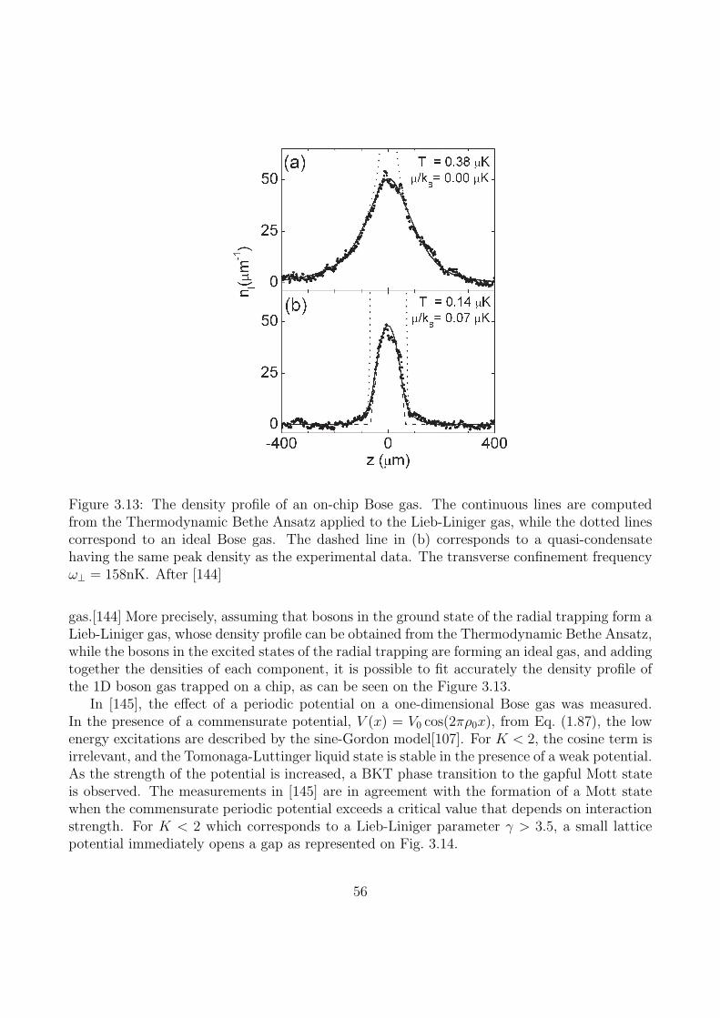
Figure 3.13: The density profile of an on-chip Bose gas. The continuous lines are computedfrom the Thermodynamic Bethe Ansatz applied to the Lieb-Liniger gas, while the dotted linescorrespond to an ideal Bose gas. The dashed line in (b) corresponds to a quasi-condensatehaving the same peak density as the experimental data. The transverse confinement frequencyω⊥ = 158nK. After [144]
gas.[144] More precisely, assuming that bosons in the ground state of the radial trapping form aLieb-Liniger gas, whose density profile can be obtained from the Thermodynamic Bethe Ansatz,while the bosons in the excited states of the radial trapping are forming an ideal gas, and addingtogether the densities of each component, it is possible to fit accurately the density profile ofthe 1D boson gas trapped on a chip, as can be seen on the Figure 3.13.
In [145], the effect of a periodic potential on a one-dimensional Bose gas was measured.In the presence of a commensurate potential, V (x) = V0 cos(2πρ0x), from Eq. (1.87), the lowenergy excitations are described by the sine-Gordon model[107]. For K < 2, the cosine term isirrelevant, and the Tomonaga-Luttinger liquid state is stable in the presence of a weak potential.As the strength of the potential is increased, a BKT phase transition to the gapful Mott stateis observed. The measurements in [145] are in agreement with the formation of a Mott statewhen the commensurate periodic potential exceeds a critical value that depends on interactionstrength. For K < 2 which corresponds to a Lieb-Liniger parameter γ > 3.5, a small latticepotential immediately opens a gap as represented on Fig. 3.14.
56

Figure 3.14: The phase diagram of a Bose gas under a periodic potential in the plane oflattice depth V0 and inverse Lieb-Liniger parameter. The solid line is the prediction from thesine-Gordon theory, while the dashed line is from the Bose-Hubbard model[146]. For stronginteraction and weak lattice depth, the sine-Gordon model describes the phase transition. Theinset shows the behavior of the gap as a function of the lattice depth. The solid line is theprediction from the sine-Gordon model (2.54), and the dashed line the result for free fermions.After [145]
57

Part II
Quantum magnetism
58
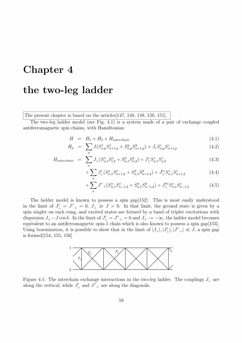
Chapter 4
the two-leg ladder
The present chapter is based on the articles[147, 148, 149, 150, 151].
The two-leg ladder model (see Fig. 4.1) is a system made of a pair of exchange coupledantiferromagnetic spin chains, with Hamiltonian:
H = H1 +H2 +Hinterchain (4.1)
Hp =∑
n
J(Sxn,pS
xn+1,p + Sy
n,pSyn+1,p) + JzS
zn,pS
zn+1,p (4.2)
Hinterchain =∑
n
J⊥(Sxn,1S
xi,2 + Sy
n,1Syn,2) + Jz
⊥Szn,1S
zn,2 (4.3)
+∑
n
J ′⊥(S
xn,1S
xn+1,2 + Sy
n,1Syn+1,2) + J ′z
⊥Szn,1S
zn+1,2 (4.4)
+∑
n
J”⊥(Sxn,1S
xn−1,2 + Sy
n,1Syn−1,2) + J ′′z
⊥ Szn,1S
zn−1,2 (4.5)
The ladder model is known to possess a spin gap[152]. This is most easily understoodin the limit of J ′
⊥ = J”⊥ = 0, J⊥ ≫ J > 0. In that limit, the ground state is given by aspin singlet on each rung, and excited states are formed by a band of triplet excitations withdispersion J⊥−J cos k. In the limit of J ′
⊥ = J”⊥ = 0 and J⊥ → −∞, the ladder model becomesequivalent to an antiferromagnetic spin-1 chain which is also known to possess a spin gap[153].Using bosonization, it is possible to show that in the limit of |J⊥|, |J ′
⊥|, |J”⊥| ≪ J , a spin gapis formed[154, 155, 156]
⊥J’
⊥J
⊥J"1
2
Figure 4.1: The interchain exchange interactions in the two-leg ladder. The couplings J⊥ arealong the vertical, while J ′
⊥ and J”⊥ are along the diagonals.
59
4.1 Bosonization
4.1.1 General case
Starting from the boson representation of the single chain, and using Eqs. (1.66)–(1.67) oneobtains[154, 155, 156] the following bosonized representation of the two-leg ladder model:
Hp =
∫
dx
2π
[
upKp(πΠp)2 +
upKp
(∂xφp)2
]
− 2∆p
(2πα)2
∫
dx cos 4φp (4.6)
Hinterchain =
∫ [
2g1(2πa)2
cos(θ1 − θ2) +2g2
(2πa)2cos 2(φ1 − φ2) +
2g3(2πa)2
cos 2(φ1 + φ2)
]
dx
+Jz⊥a
∫
dx∂xφ1∂xφ2
π2(4.7)
Near the XY symmetric point, the coupling constants are given by:
g1 = π(J⊥ − J ′⊥ − J”⊥)a
g2 = (Jz⊥ − J ′z
⊥ − J ′′z⊥ )a
g3 = (Jz⊥ − J ′z
⊥ − J ′′z⊥ )a (4.8)
More generally, the amplitudes are renormalized by interactions. It is convenient to rewritethe Hamiltonian in terms of the fields:
φa =φ1 − φ2√
2, φs =
φ1 + φ2√2
(4.9)
which yields:
H = Hs +Ha
Ha =
∫
dx
2π
[
uaKa(πΠa)2 +
uaKa
(∂xφa)2
]
+2g3
(2πα)2
∫
dx cos(√8φa) +
2g1(2πα)2
∫
dx cos(√2θa)
Hs =
∫
dx
2π
[
usKs(πΠs)2 +
usKs
(∂xφs)2
]
+2g2
(2πα)2
∫
dx cos(√8φs) (4.10)
Where:
us = u
(
1 +KJz
⊥a
2πu
)
, Ks = K
(
1− KJz⊥a
2πu
)
ua = u
(
1− KJz⊥a
2πu
)
, Ka = K
(
1 +KJz
⊥a
2πu
)
(4.11)
60
It is worthwhile to note that the Hamiltonian 4.10 was obtained previously in a bosonizationstudy of the spin-1 chain[23], in which the spin-1 operators were represented as a symmetriccombination of spins-1/2. That result hints that spin-1 chains and two-leg ladders shouldpresent similar physical properties at low energy.
The phase diagram can be obtained from the self-consistent harmonic approximation[154]or the renormalization group[156]. For Ks < 1, the field φs becomes long range ordered, andthe Hamiltonian Hs has a gap in its excitation spectrum. In the Hamiltonian Ha as discussedin [155, 156] at least one of the operators is relevant so that the Hamiltonian is always gapped.Two phases are possible, one with φa long range ordered, and the other with θa long rangeordered. The different regimes are represented on the tables4.1 and 4.2 . The phases arenamed according to the terminology of the paper by H. J. Schulz[157]. In the phase calledXY 1 the correlations of S+
1 − sign(J⊥)S+2 are quasi-long range ordered. In the phase called
XY 2, the correlations of Sz1 − sign(Jz
⊥)Sz2 are long range ordered. In the singlet phase and
the Haldane gap phase, all the local operators have only short range order correlations. It ispossible however to construct a non-local order parameter[158] for these phases analogous tothe VBS order parameter[159, 160, 161] of the spin-1 chain. We will consider first the case ofJ⊥ − J ′
⊥ − J”⊥ < 0, where the Haldane gap phase is expected. The VBS order parameter C isa nonlocal order parameter defined for a spin-1 chain as:
C = lim|k−j|→∞
〈Szk exp(iπ
∑
k<n<j
Szn)S
zj 〉 (4.12)
In the Haldane gap phase, all the spin-spin correlation functions decay exponentially but C 6= 0.A non-zero VBS order parameter indicates that if all the sites where Sz
n = 0 are removed froma spin-1 antiferromagnetic chain the remaining (“squeezed”) chain has antiferromagnetic order.For our ladder system, the VBS order parameter takes the form[162, 147]:
Oodd = lim|k−j|→∞
〈(Szk,1 + Sz
k,2) exp
[
iπ∑
k<n<j
(Sn,1 + Szn,2)
]
(Szj,1 + Sz
j,2)〉 (4.13)
To derive a representation of the string operator, we first use the identity: exp(iπ(Sz1+S
z2)) =
− exp(iπ(Sz1 − Sz
2)), yielding:
∏
k<n<j
exp(iπ(Sz1 + Sz
2)) = (−)j−k−1 exp(∑
k<n<j
iπ(Sz1 − Sz
2)), (4.14)
which is straightforwardly bosonized in the form (−)k−j cos√2(φa(ka) − φa(ja)). Using the
bosonized expression of Sz1 + Sz
2 = Sz, the VBS order parameter is obtained in the form:
Oodd ∝ lim|x−y|→∞
〈cos√2φs(x) cos
√2φs(y)〉 = (〈cos
√2φs〉)2 (4.15)
Since in the Haldane gap phase, 〈φs〉 = 0 (see table 4.1) the VBS order parameter is non-zero. Turning to the case of J⊥ − J ′
⊥ − J”⊥ > 0, we have to consider another VBS-like order
61
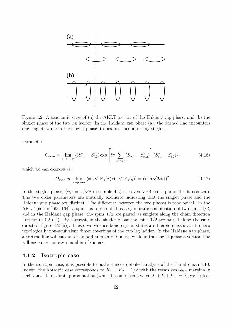
(a)
(b)
Figure 4.2: A schematic view of (a) the AKLT picture of the Haldane gap phase, and (b) thesinglet phase of the two leg ladder. In the Haldane gap phase (a), the dashed line encountersone singlet, while in the singlet phase it does not encounter any singlet.
parameter:
Oeven = lim|i−j|→∞
〈(Szi,1 − Sz
i,2) exp
[
iπ∑
i<n<j
(Sn,1 + Szn,2)
]
(Szj,1 − Sz
j,2)〉, (4.16)
which we can express as:
Oeven ∝ lim|x−y|→∞
〈sin√2φs(x) sin
√2φs(y)〉 = (〈sin
√2φs〉)2 (4.17)
In the singlet phase, 〈φs〉 = π/√8 (see table 4.2) the even VBS order parameter is non-zero.
The two order parameters are mutually exclusive indicating that the singlet phase and theHaldane gap phase are distinct. The difference between the two phases is topological. In theAKLT picture[163, 164], a spin-1 is represented as a symmetric combination of two spins 1/2,and in the Haldane gap phase, the spins 1/2 are paired as singlets along the chain direction(see figure 4.2 (a)). By contrast, in the singlet phase the spins 1/2 are paired along the rungdirection figure 4.2 (a)). These two valence-bond crystal states are therefore associated to twotopologically non-equivalent dimer coverings of the two leg ladder. In the Haldane gap phase,a vertical line will encounter an odd number of dimers, while in the singlet phase a vertical linewill encounter an even number of dimers.
4.1.2 Isotropic case
In the isotropic case, it is possible to make a more detailed analysis of the Hamiltonian 4.10.Indeed, the isotropic case corresponds to K1 = K2 = 1/2 with the terms cos 4φ1,2 marginallyirrelevant. If, in a first approximation (which becomes exact when J⊥+J
′⊥+J”⊥ = 0), we neglect
62
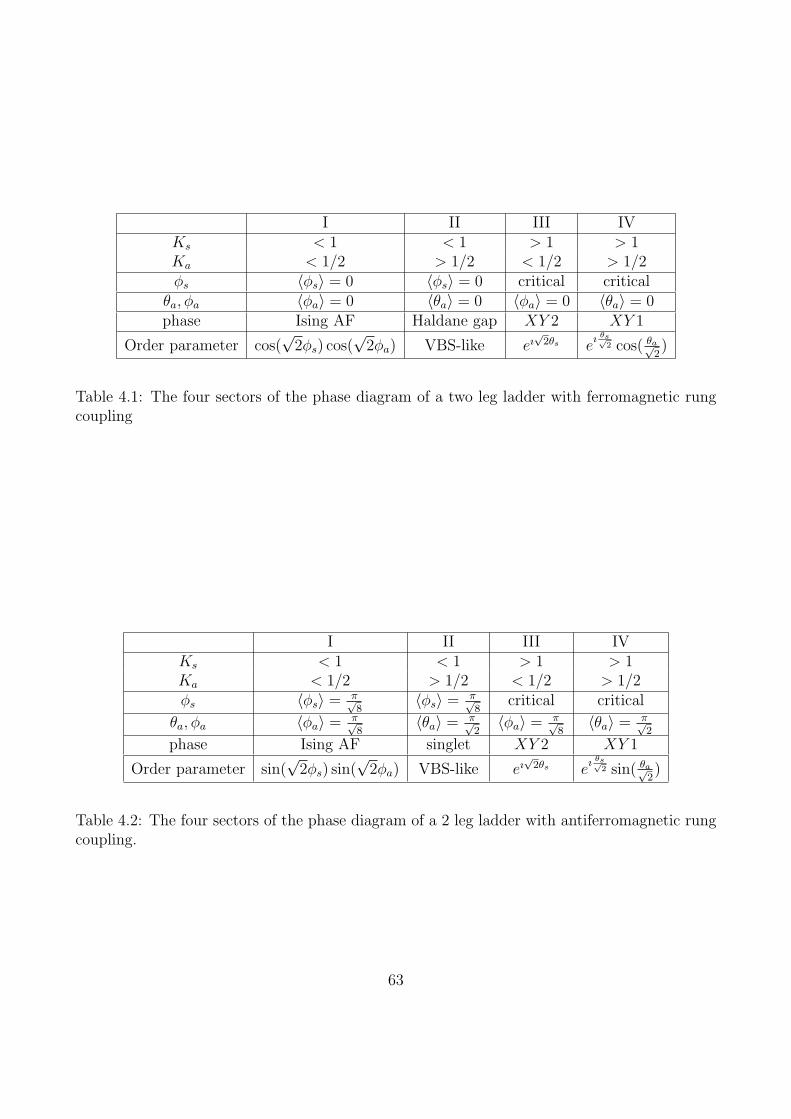
I II III IVKs < 1 < 1 > 1 > 1Ka < 1/2 > 1/2 < 1/2 > 1/2φs 〈φs〉 = 0 〈φs〉 = 0 critical critical
θa, φa 〈φa〉 = 0 〈θa〉 = 0 〈φa〉 = 0 〈θa〉 = 0phase Ising AF Haldane gap XY 2 XY 1
Order parameter cos(√2φs) cos(
√2φa) VBS-like eı
√2θs e
ı θs√2 cos( θa√
2)
Table 4.1: The four sectors of the phase diagram of a two leg ladder with ferromagnetic rungcoupling
I II III IVKs < 1 < 1 > 1 > 1Ka < 1/2 > 1/2 < 1/2 > 1/2φs 〈φs〉 = π√
8〈φs〉 = π√
8critical critical
θa, φa 〈φa〉 = π√8
〈θa〉 = π√2
〈φa〉 = π√8
〈θa〉 = π√2
phase Ising AF singlet XY 2 XY 1
Order parameter sin(√2φs) sin(
√2φa) VBS-like eı
√2θs e
ı θs√2 sin( θa√
2)
Table 4.2: The four sectors of the phase diagram of a 2 leg ladder with antiferromagnetic rungcoupling.
63
all the marginal operators in the Hamiltonian 4.10 we can make the rescaling φa → φa/√2,
θa →√2θa and fermionize the resulting Hamiltonian[162]. It is convenient to rewrite the
Hamiltonian using a Majorana fermion representation:1
H = −iu2
2∑
a=0r=±
∫
dxrζr,a∂xζr,a (4.18)
+im
∫
dx
(
3∑
a=1
ζa,+ζa,− − 3ζ0,+ζ0,−
)
, (4.19)
showing that the spectrum consists of a triplet of Majorana fermions of mass m and a singletMajorana fermion of mass −3m. Moreover, using the relation between massive Majoranafermions and the Ising model, a representation of the spin-operators can be derived.[162] If onewrites: Sn,p = Jp(x) + (−)nn(x), then one has:
Mx = nx1 + nx
2 = λσ1µ2σ3σ0 (4.20)
My = ny1 + ny
2 = λµ1σ2σ3σ0 (4.21)
Mz = nz1 + nz
2 = λσ1σ2µ3σ0 (4.22)
mx = nx1 − nx
2 = λµ1σ2µ3µ0 (4.23)
my = ny1 − ny
2 = λσ1µ2µ3µ0 (4.24)
mz = nz1 − nz
2 = λµ1µ2σ3µ0 (4.25)
Using the results of[74], this allows the calculation of zero temperature correlation functions interms of Painleve III functions. The results of such computations are in good agreement withnumerical work[166]. The uniform component of the magnetization can be directly expressedin terms of the Majorana fermion operators as:
Jx1 + Jx
2 =i
2(ζ+,2ζ+,3 + ζ−,2ζ−,3) (4.26)
Jy1 + Jy
2 =i
2(ζ+,3ζ+,1 + ζ−,3ζ−,1) (4.27)
Jy1 + Jy
2 =i
2(ζ+,1ζ+,2 + ζ−,1ζ−,3) (4.28)
Jx1 − Jx
2 =i
2(ζ+,0ζ+,1 + ζ−,0ζ−,1) (4.29)
Jy1 − Jy
2 =i
2(ζ+,0ζ+,2 + ζ−,0ζ−,2) (4.30)
Jz1 − Jz
2 =i
2(ζ+,0ζ+,3 + ζ−,0ζ−,3) (4.31)
1This technique is also applicable in the presence of biquadratic spin-spin interaction[165].
64
4.2 Semi-infinite ladder
In the case of the semi-infinite spin-1 chain, it has been shown, by considering the topologicalterm in the path integral representation,[167] that in the Haldane gap phase, spin-1/2 edgestates would be obtained. A simple picture of this result can be obtained by considering theAKLT ground state: cutting the chain anywhere will necessarily cut a dimer a leave one freespin-1/2. The same question can be asked in the case of the two-leg ladder, i. e. whethera semi-infinite ladder will present edge states. In fact, the edge states are only obtained[149]when the ladder is in the Haldane gap state with Oodd 6= 0. To discuss that result, we firstneed to consider the case of a spin-1/2 chain with open boundary conditions.[168, 169]
4.2.1 Open boundary conditions in a spin-1/2 chain
Let us first consider the spin-1/2 chain with open boundary conditions in the XY limit. TheHamiltonian reads:
H = J
+∞∑
n=1
(S+n S
−n+1 + S−
n S+n+1), (4.32)
and becomes, after the Jordan-Wigner transformation (1.57):
J = −J+∞∑
n=1
(c†ncn+1 + c†n+1cn), (4.33)
giving the eigenvalue equations:
Ecn = −J(cn+1 + cn−1), (n ≥ 2) (4.34)
Ec1 = −Jc2, (4.35)
These equations can be reduced to a single equation by introducing a fictitious site 0 such thatc0 = 0. The Hamiltonian (4.33) is then diagonalized by introducing:
cn =
√
2
N
∑
k>0
ck sin(kn), (4.36)
H =∑
k>0
ǫ(k)c†kck. (4.37)
Taking the continuum limit of that Hamiltonian, we find:
cn√a
= eiπ2nψ+(na)− e−iπ
2nψ+(−na), (4.38)
H = −iv∫ ∞
−∞dxψ†
+∂xψ+ (4.39)
65
We notice that we can bring that representation to the same form as in the case of the infinitesystem simply by introducing ψ−(x) = −ψ+(−x). In terms of the bosonized representation,the latter condition is simply φ+(x) + φ−(−x) = π. Using the equation of motions of thechiral fields, φr(x, t) = φr(x − rut, 0) = φr(0, t − rx/u) that condition can be rewritten asφ(0, t) = π/2 ∀t. So we see that the bosonized representation of a semi-infinite XY spin chainis obtained simply by imposing a boundary condition φ(0, t) = π/2. Such boundary conditioncan be viewed as the condition that sin 2φ(0, t) = 0 i. e. that the staggered component ofthe magnetization (1.67) vanishes. Simultaneously, the staggered dimerization operator (1.68)takes at the edge of the chain its maximal value. In the interacting case, the boundary conditionis preserved, and the general XXZ spin-1/2 chain bosonized Hamiltonian is:
H =
∫ ∞
0
dx
2π
[
uK(πΠ)2 +u
K(∂xφ)
2]
− 2∆
(2πα)2
∫
dx cos 4φ (4.40)
φ(0) = π/2 (4.41)
Indeed, with the boundary condition φ(0) = π/2, we ensure that the staggered component of themagnetization vanishes on the edge, irrespective of interaction. By defining φ(x) = π/2+
√Kφ
and θ(x) = ˜theta(x)/√K, we can transform the Hamiltonian (4.40) into a non-interacting
Hamiltonian. We then find that the boundary condition φ(0, t) = 0 is solved by introducingthe chiral field φ+(x, t) = φ+(x− ut, 0) and writing:
φ(x, t) =1
2(φ+(x− ut)− φ+(−x− ut)); θ(x, t) = −1
2(φ+(x− ut) + φ+(−x− ut)), (4.42)
so that:
φ(x, t) =π
2+
√K
2(φ+(x− ut)− φ+(−x− ut)) (4.43)
θ(x, t) = − 1
2√K
(φ+(x− ut) + φ+(−x− ut)) (4.44)
With Eq. (4.43), we find that in a semi-infinite chain, 〈eiλθ(x)+µφ(x)〉 = 0 and 〈eiλφ(x)〉 =eiλ
π2 [α/(2x)]λ
2K/4. In the absence of an external magnetic field, this leads to 〈Sx,y,zn 〉 = 0.
When a magnetic field is applied along the z direction, kF 6= π/2 and Friedel oscillations ofthe magnetization appear. In the case of a spin-1/2 chain, we can turn the boundary conditionφ(0) = π/2 into the simpler boundary condition φ(0) = 0 provided that we change the sign ofsin 2φ and cos 2φ in Eqs.(1.66)– (1.68).
4.2.2 Two-leg ladder with open boundary conditions
We are now considering a semi-infinite ladder model with open boundary conditions. We canstill apply bosonization, but the Hamiltonian (4.10) is now restricted to x > 0 with boundaryconditions φs(0) = 0 and φa(0) = 0. The ladder can still be fermionized, but a relation nowexists between the right moving and the left moving fields[149]:
ζ+,n(0) = ζ−,n(0), (4.45)
66
for 0 ≤ n ≤ 3. To find the eigenstates of the fermionized Hamiltonian, it is sufficient to considerfor each n the 1D Dirac equation:
(−iuσ3∂x +mnσ2)Ψn(x) = EΨn(x), (4.46)
where Ψ(x) is a two-component column vector,
Ψn(x) =
(
ζn,+ζn,−
)
. (4.47)
The general solution taking into account the boundary condition (4.45) reads:
Ψn (x, t) =1√2L
∑
k>0
ak
(
cos (kx+ θk) + i sin (kx)cos (kx+ θk)− i sin (kx)
)
e−iǫkt +H.c.
+
√
mn
u
(
11
)
e−mnx/u θ (mn) ηn,
(4.48)where ǫ(k) =
√
(uk)2 +m2, ak is a fermion annihilation operator, eiθk = (uk + im)/ǫ(k), andη is a Majorana fermion operator. The Majorana fermion is present only when mn > 0. Asa result, in the case of a ladder with J⊥ − J ′
⊥ − J ′′⊥ < 0, a triplet of Majorana fermion bound
states is formed near the edge, while in the opposite case, a singlet Majorana fermion boundstate is formed.
In the case where a triplet of Majorana fermions is formed, since from (4.26) the uniformmagnetization is:
Mc =
∫ ∞
0
dx(J+,c + J−,c) = iǫabc2
∫
dx(ζ+,aζ+,b + ζ−,aζ−,b), (4.49)
after integration, a contribution to the magnetization:
Mc =i
2ǫabcηaηb, (4.50)
where ηa are the Majorana fermion operators associated with the bound state. Eq. (4.50) isprecisely the representation of a spin-1/2 in terms of Majorana fermion operators[170]. Thepresence of a spin-1/2 excitation at the edge in a ladder with ferromagnetic coupling can beunderstood from the limit of infinite ferromagnetic rung coupling where the ladder becomes aspin-1 chain. It is known that the spin-1 chain in the Haldane gap phase with open boundarycondition possesses spin-1/2 edge modes[167]. Those edge modes can be understood from theAKLT picture[163, 164]. In that picture, each spin-1 is decomposed into two spins 1/2. Thespins 1/2 are then paired with their nearest neighbors in singlets so that one of the spins ispaired with a spin on the left, and the other with a spin on the right, thus leaving an infinitechain translationally invariant. It is clear in that picture that cutting the spin 1 chain anywhere,will leave a free spin-1/2 edge state.
The Majorana fermion representation also allows the calculation of the staggered magnetiza-tion and the staggered dimerization in the semi-infinite two-leg ladder. Indeed, as we have seenin Sec. 2.2.2, massive Majorana fermions on an infinite line are related with the one-dimensional
67
quantum Ising chain and the two-dimensional classical Ising model. In the case of a semi-infiniteline, the equivalence persists, but the boundary conditions on the Majorana fermions translateinto boundary conditions on the Ising degrees of freedom. Fortunately, the latter conditionsare quite simple. When the Majorana fermions obey the boundary condition ζ+(0) = ζ−(0),the spins σ satisfy the free boundary condition, whereas when the Majorana fermions obeyζ+(0) = −ζ−(0), the spins satisfy the fixed boundary conditions σ(0) = 1.[171, 172, 173] Sinceunder a duality transformation the order (σ) and the disorder (µ) parameter are exchanged,free boundary conditions for the spin σ translate into fixed boundary conditions for µ and vice-versa. In the Ising language, the semi-infinite ladder is therefore equivalent to four decoupledsemi-infinite Ising models with free boundary conditions. A positive mass for the Majoranafermions corresponds to a two-dimensional Ising model below its critical temperature. Withfree boundary conditions, the localized Majorana fermion mode corresponds to a domain wallbound to the edge in the Ising model. When the mass is negative, the Ising model is abovethe critical temperature, and no domain wall is attached to the edge. Using the results from[171, 172, 173, 174, 175], we obtain the following expression for the staggered magnetization:
〈nz+ (x)〉 ∼
(
m3t |ms|a4v3t vs
)1/8
e−mtx/vtH2
(
mtx
vt
)
G
(
mtx
vt
)
G
( |ms|xvs
)
, (4.51)
where the functions G and H can be expressed terms of a solution to the Painleve III differentialequation:
1
η
d2η
dθ2=
(
1
η
dη
dθ
)2
− 1
θη
dη
dθ+ η2 − 1
η2. (4.52)
with boundary conditions on η :
η(θ) ∼ −θ[
lnθ
4+ γE
]
(θ → 0)
η(θ) ∼ 1− K0(2θ)
2π(θ → ∞), (4.53)
γE being the Euler’s constant. The functions G and H are defined by:
G(y) = η−1/4(y) exp
[
∫ ∞
y
dθ
θ
8η−2(θ)
(
(1− η2(θ))2 −(
dη
dθ
)2)
− 1
2(1− η(θ))
]
H(y) = η1/4(y) exp
[
∫ ∞
y
dθ
θ
8η−2(θ)
(
(1− η2(θ))2 −(
dη
dθ
)2)
− 1
2(η−1(θ)− 1)
]
.(4.54)
There is an apparent paradox in having a non vanishing staggered magnetization in theabsence of an external magnetic field since this violates the SU(2) invariance of the model.Actually, the Eq. (4.51) is only valid when Sz
tot. = 0. Such a state is only invariant underrotations around the z-axis, and can sustain a staggered magnetization, as has been observedin DMRG calculations[176, 177]. A staggered dimerization is also present. Using the bosonized
68
expression (1.68), and the mapping to the Ising spins, we find that the staggered dimerizationis ǫ+ ∼ µ1µ2µ3µ0. The expectation value is then:
〈ǫ+ (x)〉 ∼(
m3t |ms|a4v3t vs
)1/8
e−3mtx/vtG3
(
mtx
vt
)
G
( |ms|xvs
)
. (4.55)
for ferromagnetic rung interaction, and:
〈ǫ+ (x)〉 ∼( |mt|3msa
4
v3t vs
)1/8
e−msx/vtG3
( |mt|xvt
)
G
(
msx
vs
)
, (4.56)
for antiferromagnetic rung interaction.We can also obtain the staggered magnetization profile when the edge spin is polarized by
an external magnetic field. We find in the ferromagnetic rung case:
〈nx+ (x)〉 ∼ e−|mt|x/vtG3
( |mt|xvt
)
G
(
msx
vs
)
, (4.57)
and in the antiferromagnetic rung case:
〈nx+ (x)〉 ∼ e−2mtx/vt−|ms|x/vsG3
(
mtx
vt
)
G
( |ms|xvs
)
, (4.58)
4.3 Ladders under a magnetic field
Until now, we have restricted ourselves to ladders in zero external magnetic field. In thepresence of an applied field, one must add a term:
Hfield = −hπ
∫
dx∂x(φ1 + φ2) (4.59)
= −h√2
π
∫
dx∂xφs. (4.60)
When Hs is gapped in zero magnetic field, that term induces a commensurate-incommensuratetransition[178, 179]. For h > hc, the Hamiltonian Hs + Hfield has a Luttinger liquid groundstate with gapless spectrum[180, 181, 182]. The Singlet or Haldane phase are turned into theXY 1 phase, while the Ising antiferromagnetic phase are turned into the XY 2 phase. Thetransition is most easily understood in the SU(2) invariant limit. Indeed, in that case, we canfermionize Hs +Hfield in the form;
H =
∫
dx
[
−ius(ψ†+∂xψ+ − ψ†
−∂xψ−)dx+ i∆s
∫
(ψ†+ψ− − ψ†
−ψ+)− h(ψ†+ψ+ + ψ†
−ψ−)
]
,(4.61)
and the energy of excitations is simply E±(k) = ±√
(usk)2 +∆2s −hs. When |hs| < |∆s|, there
are no zero energy excitations, and the system remains gapped. When |hs| > |∆s|, a fermion or
69
hole Fermi surface is formed with a Fermi momentum kF =√
h2s −∆2s/us. This implies that
the ladder is becoming magnetized, with a magnetization proportional to kF . Moreover, we canderive a bosonized description of the fermions, which leads to a Hamiltonian of the form (1.27)for the φs modes,
H =
∫
dx
2π
[
u∗s(h)K∗s (h)(πΠs)
2 +u∗s(h)
K∗s (h)
(∂xφs)2
]
(4.62)
Since the fermions are non-interacting, we have K∗s = 1 and u∗s(h) = us
√
1− (∆s/h)2 inEq.(4.59). Away from the non-interacting point Ks = 1, it has been shown[183] that when hgoes to the critical field hc the Tomonaga-Luttinger exponent Ks goes to 1. For the generalsine-Gordon model, the velocity and exponent were derived in[184]. Right at the critical field,the dispersion of the excitations is quadratic, and the system is at a z = 2 quantum criticalpoint[185]. The spin-spin correlation functions in the magnetized phase have been derivedexplicitly in [181, 182].
Such a transition can be observed in organic two-leg ladders such as BPCB.[186] In sucha system however, the rung coupling is larger than the leg coupling, and the weak couplingbosonization analysis is not justified. However, in the limit of J⊥ ≫ J , an effective XXZ spinchain model can be derived to describe the low energy physics of the model.[187, 188] In thederivation, one first neglects J and considers simply the eigenstates of a simple dimer. Theyare formed of a singlet of energy −3J⊥/4 and a triplet with energies J⊥/4 + h, J⊥, J⊥ − h. Forh = J⊥, the singlet and the triplet with both spins polarized along the magnetic field (i. e.Sz = 1) exchange stability. Thus, one can choose a low-energy subspace formed of two states,the singlet and the Sz = 1 triplet on each rung, and apply perturbation theory to derive theeffective Hamiltonian. The two states can be represented with a pseudospin τ z with τ z = −1/2in the singlet state and τ z = 1/2 in the triplet state so that Sz = 1/2 + τ z. The effective spinchain Hamiltonian reads:
H = −J∑
n
(τxnτxn+1 + τ ynτ
yn+1 +
1
2τ znτ
zn+1)− (h− J⊥)
∑
n
τ zn , (4.63)
and the local magnetization in the plane orthogonal to the magnetic field can be written as:
S+n,p =
(−1)pτ+n√2
(4.64)
In the partially magnetized phase, the spin chain described by the Hamiltonian (4.63) is in aTomonaga-Luttinger liquid state. With the representation (1.69), we can interpret the tripletsas hard core boson particles, and the singlet as a particle vacuum. In that picture, the mag-netized ladder can be viewed as a Tomonaga-Luttinger liquid of hard-core bosons. Using theBethe Ansatz solution of the XXZ chain, (4.63) the velocity and Tomonaga-Luttinger expo-nents have been derived[182]. Moreover, when the magnetization is at half the saturation value,τ zn = 0 and the amplitudes in Eqs. (1.95) are given by (1.97). In the intermediate case of BPCB,where J‖ = 3.55 K and J⊥ = 12.6 K, a numerical approach is necessary. The method used in[151] is the Density Matrix Renormalization Group (DMRG).[189, 190] In its simplest version,
70
this method allows to find the ground state of a two leg ladder with open boundary conditionsand obtain equal time correlation functions. Since the low-energy physics is described by aTomonaga-Luttinger liquid model with a known representation of spin the operators, it is pos-sible to calculate the Friedel oscillations of the spin as a function of the Tomonaga-Luttingerexponent[191, 192, 193] By fitting the Friedel oscillations, the Tomonaga-Luttinger exponentcan be extracted. The velocity is extracted from the magnetic susceptibility.
In the BPCB compound, the ladders are not strictly isolated. There is an interladderexchange Jx which is smaller than the leg and rung exchanges. For sufficiently low temperature,the existence of this interladder exchange destabilizes the Tomonaga-Luttinger liquid. The spinsthen develop a long-range antiferromagnetic ordering on the ladders, and satisfy the constraintsimposed by the interladder exchange. The long range ordering is of the easy plane type, withthe spins lying in the plane orthogonal to the applied field. In a bosonization description, theeffective model that describes the coupled ladders takes the form:
H =∑
m
∫
dx
2π
[
u∗(h)K∗(h)(πΠm)2 +
u∗(h)
K∗(h)(∂xφm)
2
]
− J ′∑
〈m,m′〉Ax
0(h)
∫
dx cos(θm − θm′)(x)(4.65)
where m is the ladder index, J ′ is the interladder exchange, and Ax0(h) is an amplitude as in
Eq. (1.95). The Hamiltonian (4.65) can be treated in mean field theory.[194] The mean field is:
hMF = zJ ′Ax0(h)〈cos θm〉HMF
, (4.66)
where z is the number of nearest neighbors of a given ladder, and the mean-field Hamiltonianused to determine hMF selfconsistently reads:
HMF =
∫
dx
2π
[
u∗(h)K∗(h)(πΠ)2 +u∗(h)
K∗(h)(∂xφ)
2 − hMF
∫
dx cos θ
]
. (4.67)
such a Hamiltonian can be brought to the form (2.1) by a duality transformation and a rescaling.Using perturbation theory, it is possible to derive the critical temperature. Indeed, (4.66) canbe rewritten as:
hMF = zJ ′Ax0(h)〈TτehMF
∫
dx∫ β
0 dτ cos θ(x,τ) cos θ(0, 0)〉. (4.68)
Expanding to first order in hMF we find that the self-consistency condition is going to besatisfied at a temperature βc such that:
1 = zJ ′Ax0(h)
∫
dx
∫ βc
0
dτ〈Tτ cos θ(x, τ) cos θ(0, 0)〉. (4.69)
Using Eq. (1.56), we obtain the critical temperature.
Tc =u
2π
[
sin( π
4K
)
B2
(
1
8K, 1− 1
4K
)
· zJ′Ax
0(h)
2u
] 2K4K−1
. (4.70)
It is possible to go further and obtain also the order parameter for zero temperature usingthe results of [79]
71
mx = F (K) ·√
Ax0
(
πzJ ′Ax0
2u
) 18K−2
, (4.71)
where
F (K) =
π2
sin( π8K−1
)· 8K8K−1
[
Γ(1− 18K
)
Γ( 18K
)
]8K
8K−1
Γ(
4K8K−1
)2Γ(
16K−316K−2
)2
8K−18K−2
.
The parameters u(h), K(h), A0(h) can be obtained from DMRG calculations[151, 195, 196, 197].A comparison of the experimental transition temperature and zero temperature magnetizationwith the theoretical result is shown on Figs. 4.3 (c)-(d). For the critical temperature, the fittingparameter is J ′ = 20 mK. With that fitting parameter, the amplitude of the order parametercan be obtained. After adjusting for an overall scale, the staggered magnetization obtained inNMR can be compared with the theoretical prediction. Neutron scattering allows to measureprecisely the amplitude of the order parameter, without adjustable overall amplitude.
4.4 Ladders with Dzyaloshinskii-Moriya interaction
Besides the Heisenberg exchange interaction, localized spin systems can also present the Dzyaloshinskii-Moriya interaction[198, 199]. This interaction originates in relativistic effects that give rise tospin orbit interactions. In a tight binding formulation, the spin-orbit interaction takes the formof a spin-dependent hopping integral:
H = −∑
i,j
Tij;αβc†i,αcj,β, (4.72)
Tij;αβ = t0ijδαβ + tij · σαβ (4.73)
When this hopping integral is inserted in the Hubbard model[200, 201, 202] and second orderperturbation theory is used to eliminate the doubly occupied sites, it gives rise, besides theHeisenberg exchange term, to a spin-spin interaction of the form:
∑
ij
Dij · (Si × Sj) + Aαβij S
αi S
βj , (4.74)
where Dij is the Dzyaloshinskii-Moriya (DM) vector and Aαβij is the Kaplan-Shekhtman-Entin-
Wolfmann-Aharony (KSEA) tensor. A necessary condition for the presence of a DM interactionis the absence of an inversion center in the middle of the bond ij. When the on-site interactionspossess the full SU(2) symmetry, the KSEA tensor and the Dzyaloshinskii-Moriya vector arenot independent from each other.[200, 201, 202] The interaction (4.74) can be rewritten in theform:
∑
ij
DSαi Rαβ
ij Sβj , (4.75)
72
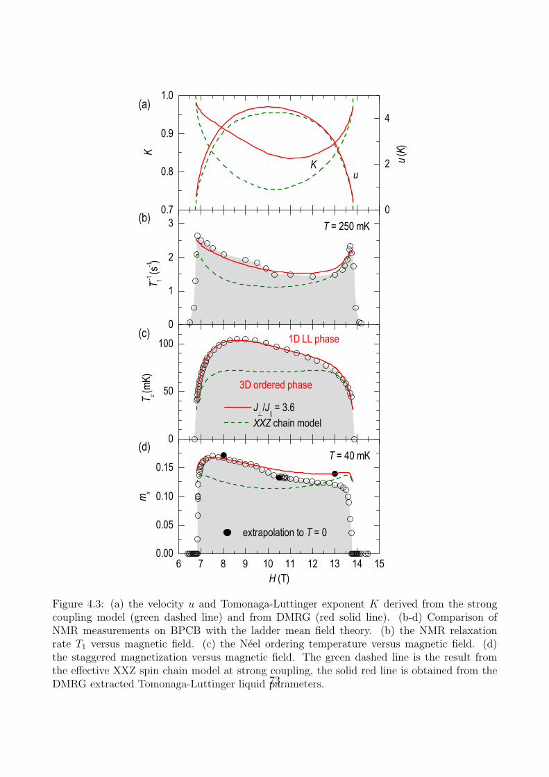
Figure 4.3: (a) the velocity u and Tomonaga-Luttinger exponent K derived from the strongcoupling model (green dashed line) and from DMRG (red solid line). (b-d) Comparison ofNMR measurements on BPCB with the ladder mean field theory. (b) the NMR relaxationrate T1 versus magnetic field. (c) the Neel ordering temperature versus magnetic field. (d)the staggered magnetization versus magnetic field. The green dashed line is the result fromthe effective XXZ spin chain model at strong coupling, the solid red line is obtained from theDMRG extracted Tomonaga-Luttinger liquid parameters.73
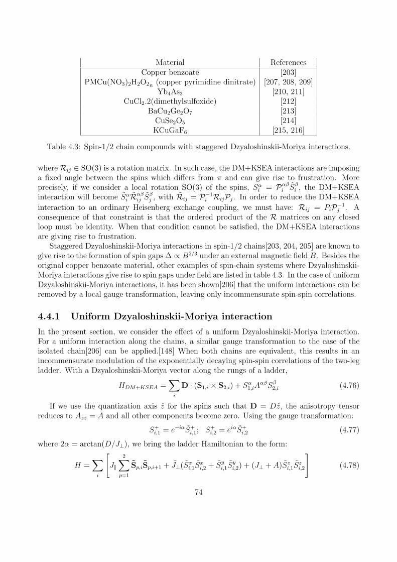
Material ReferencesCopper benzoate [203]
PMCu(NO3)2H2O2n (copper pyrimidine dinitrate) [207, 208, 209]Yb4As3 [210, 211]
CuCl2.2(dimethylsulfoxide) [212]BaCu2Ge2O7 [213]CuSe2O5 [214]KCuGaF6 [215, 216]
Table 4.3: Spin-1/2 chain compounds with staggered Dzyaloshinskii-Moriya interactions.
where Rij ∈ SO(3) is a rotation matrix. In such case, the DM+KSEA interactions are imposinga fixed angle between the spins which differs from π and can give rise to frustration. Moreprecisely, if we consider a local rotation SO(3) of the spins, Sα
i = Pαβi Sβ
i , the DM+KSEAinteraction will become Sα
i Rαβij S
βj , with Rij = P−1
i RijPj. In order to reduce the DM+KSEA
interaction to an ordinary Heisenberg exchange coupling, we must have: Rij = PiP−1j . A
consequence of that constraint is that the ordered product of the R matrices on any closedloop must be identity. When that condition cannot be satisfied, the DM+KSEA interactionsare giving rise to frustration.
Staggered Dzyaloshinskii-Moriya interactions in spin-1/2 chains[203, 204, 205] are known togive rise to the formation of spin gaps ∆ ∝ B2/3 under an external magnetic field B. Besides theoriginal copper benzoate material, other examples of spin-chain systems where Dzyaloshinskii-Moriya interactions give rise to spin gaps under field are listed in table 4.3. In the case of uniformDzyaloshinskii-Moriya interactions, it has been shown[206] that the uniform interactions can beremoved by a local gauge transformation, leaving only incommensurate spin-spin correlations.
4.4.1 Uniform Dzyaloshinskii-Moriya interaction
In the present section, we consider the effect of a uniform Dzyaloshinskii-Moriya interaction.For a uniform interaction along the chains, a similar gauge transformation to the case of theisolated chain[206] can be applied.[148] When both chains are equivalent, this results in anincommensurate modulation of the exponentially decaying spin-spin correlations of the two-legladder. With a Dzyaloshinskii-Moriya vector along the rungs of a ladder,
HDM+KSEA =∑
i
D · (S1,i × S2,i) + Sα1,iA
αβSβ2,i (4.76)
If we use the quantization axis z for the spins such that D = Dz, the anisotropy tensorreduces to Azz = A and all other components become zero. Using the gauge transformation:
S+i,1 = e−iαS+
i,1; S+i,2 = eiαS+
i,2 (4.77)
where 2α = arctan(D/J⊥), we bring the ladder Hamiltonian to the form:
H =∑
i
[
J‖
2∑
p=1
Sp,iSp,i+1 + J⊥(Sxi,1S
xi,2 + Sy
i,1Syi,2) + (J⊥ + A)Sz
i,1Szi,2
]
(4.78)
74
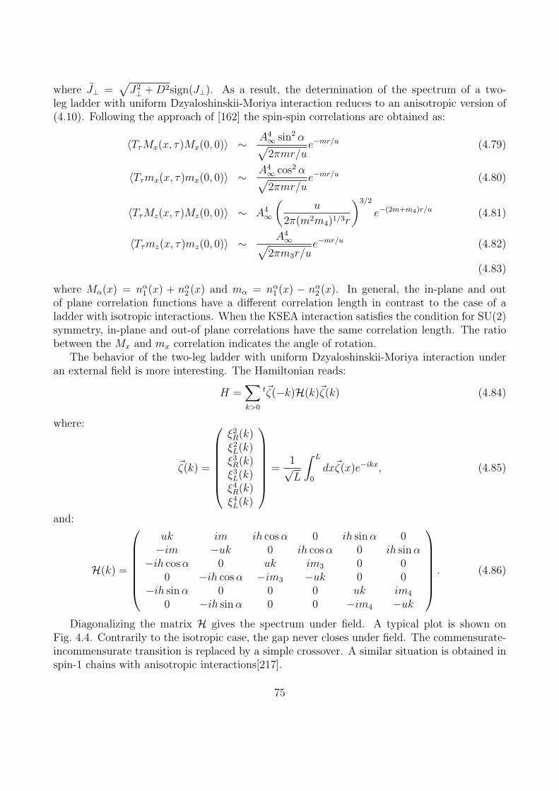
where J⊥ =√
J2⊥ +D2sign(J⊥). As a result, the determination of the spectrum of a two-
leg ladder with uniform Dzyaloshinskii-Moriya interaction reduces to an anisotropic version of(4.10). Following the approach of [162] the spin-spin correlations are obtained as:
〈TτMx(x, τ)Mx(0, 0)〉 ∼ A4∞ sin2 α
√
2πmr/ue−mr/u (4.79)
〈Tτmx(x, τ)mx(0, 0)〉 ∼ A4∞ cos2 α
√
2πmr/ue−mr/u (4.80)
〈TτMz(x, τ)Mz(0, 0)〉 ∼ A4∞
(
u
2π(m2m4)1/3r
)3/2
e−(2m+m4)r/u (4.81)
〈Tτmz(x, τ)mz(0, 0)〉 ∼ A4∞
√
2πm3r/ue−mr/u (4.82)
(4.83)
where Mα(x) = nα1 (x) + nα
2 (x) and mα = nα1 (x) − nα
2 (x). In general, the in-plane and outof plane correlation functions have a different correlation length in contrast to the case of aladder with isotropic interactions. When the KSEA interaction satisfies the condition for SU(2)symmetry, in-plane and out-of plane correlations have the same correlation length. The ratiobetween the Mx and mx correlation indicates the angle of rotation.
The behavior of the two-leg ladder with uniform Dzyaloshinskii-Moriya interaction underan external field is more interesting. The Hamiltonian reads:
H =∑
k>0
t~ζ(−k)H(k)~ζ(k) (4.84)
where:
~ζ(k) =
ξ2R(k)ξ2L(k)ξ3R(k)ξ3L(k)ξ4R(k)ξ4L(k)
=1√L
∫ L
0
dx~ζ(x)e−ikx, (4.85)
and:
H(k) =
uk im ih cosα 0 ih sinα 0−im −uk 0 ih cosα 0 ih sinα
−ih cosα 0 uk im3 0 00 −ih cosα −im3 −uk 0 0
−ih sinα 0 0 0 uk im4
0 −ih sinα 0 0 −im4 −uk
. (4.86)
Diagonalizing the matrix H gives the spectrum under field. A typical plot is shown onFig. 4.4. Contrarily to the isotropic case, the gap never closes under field. The commensurate-incommensurate transition is replaced by a simple crossover. A similar situation is obtained inspin-1 chains with anisotropic interactions[217].
75
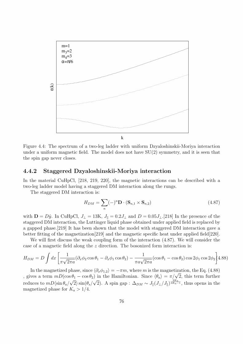
ε(k)
k
m=1
m3=2
m4=3
α=π/6
Figure 4.4: The spectrum of a two-leg ladder with uniform Dzyaloshinskii-Moriya interactionunder a uniform magnetic field. The model does not have SU(2) symmetry, and it is seen thatthe spin gap never closes.
4.4.2 Staggered Dzyaloshinskii-Moriya interaction
In the material CuHpCl, [218, 219, 220], the magnetic interactions can be described with atwo-leg ladder model having a staggered DM interaction along the rungs.
The staggered DM interaction is:
HDM =∑
n
(−)nD · (Sn,1 × Sn,2) (4.87)
with D = Dy. In CuHpCl, J⊥ = 13K, J‖ = 0.2J⊥ and D = 0.05J⊥.[218] In the presence of thestaggered DM interaction, the Luttinger liquid phase obtained under applied field is replaced bya gapped phase.[219] It has been shown that the model with staggered DM interaction gave abetter fitting of the magnetization[219] and the magnetic specific heat under applied field[220].
We will first discuss the weak coupling form of the interaction (4.87). We will consider thecase of a magnetic field along the z direction. The bosonized form interaction is:
HDM = D
∫
dx
[
1
π√2πa
(∂xφ2 cos θ1 − ∂xφ1 cos θ2)−1
πa√2πa
(cos θ1 − cos θ2) cos 2φ1 cos 2φ2
]
.(4.88)
In the magnetized phase, since 〈∂xφ1,2〉 = −πm, wherem is the magnetization, the Eq. (4.88), gives a term mD(cos θ1 − cos θ2) in the Hamiltonian. Since 〈θa〉 = π/
√2, this term further
reduces to mD〈sin θa/√2〉 sin(θs/
√2). A spin gap : ∆DM ∼ J‖(J⊥/J‖)
2Ka4Ka−1 , thus opens in the
magnetized phase for Ka > 1/4.
76
In the strong coupling limit, we can use the mapping [221, 188] to an XXZ spin chain, andobtain an effective interaction:
HDM =D√2
∑
n
(−1)nτxn . (4.89)
A bosonized form of that Hamiltonian can be derived:
H =
∫
dx
2π
[
uK(πΠ)2+u
K(∂xφ)
2]
+λD
a√2
∫
dx cos θ, (4.90)
The model (4.90) possesses for K > 1/4 breathers with masses:
Mn = 2M0 sin
(
π
2
n
8K − 1
)
, (4.91)
In order to observe those breather excitations, it is not possible to rely on ESR measurementsas ESR absorption intensity is proportional to an autocorrelation function of (Sx
1 +Sx2 ), but this
operator becomes zero in the strong coupling model. However, Raman scattering can be usedto probe the breather modes. In the Fleury-Loudon approximation[222], valid for frequencies ofincoming radiation much smaller than the Mott gap of the material[223], the Raman operatortakes the form:
HR =∑
i,j
Jij(eO · nij)(eI · nij)Si · Sj, (4.92)
where nij is the unit vector connecting the sites i and j,eI the polarization vector of theincoming radiation, eO is the polarization vector of the outgoing radiation. In full generality,the amplitude Jij depends on the geometry [224] but, as in most studies [225], we take itconstant i.e. Jij = γ.
For simplicity, here we restrict ourselves to simple geometrical setups, e.g. to the XX,YY and X’Y’ geometries corresponding to eI and eO, both along the chains direction, bothperpendicular to the chains and at 45-degrees from the crystal axes (X’=X+Y, Y’=X-Y),respectively. The corresponding Raman operators can then be written as,
OXXR = γ
∑
n
(Sn,1 · Sn+1,1 + Sn,2 · Sn+1,2) , (4.93)
OY YR = γ
∑
n
Sn,1 · Sn,2 , (4.94)
OX′Y ′R =
1
2(OXX
R − OY YR ) . (4.95)
Going to the continuum limit, it is convenient to introduce a density for the Raman operator,Oαβ
R (x) so that OalphaβR =
∫
OαβR (x)dx. Using the density of Raman operator, and the standard
definition of Raman scattering intensity, we finally find that:
IR,‖(ω) =∑
n
|〈n,Pn = 0|OXXR (0)|0〉|2δ(ω − En) (4.96)
77
where |0〉 is the ground state (GS) of the system and |n,Pn〉 is the n−th excited state withPn its total momentum. Since the Raman operator is a sum over all sites, Raman scattering isconserving photon momenta. This explains why only the states with zero momenta (i.e. havingthe same momentum as the ground state) contribute to the sum (4.96).
In the following, we compute the Raman intensity for frequencies smaller than 2J⊥ usingthe strong coupling theory. We consider first the case of a field parallel to the legs in Sec. 4.4.2,and then the case of a field parallel to the rungs in Sec. 4.4.2.
Electric field along the legs
In the strong coupling limit, we can rewrite the Raman operator (4.93) as,
OXXR =
γ
2
∑
n
(τ+n τ−n+1 + τ+n+1τ
−n
+ (τ zn + 1/2)(τ zn+1 + 1/2)), (4.97)
yielding the expression:
OXXR = γ
H −HDM + (h− J⊥ − J‖/2)∑
τ znJ‖
+ const., (4.98)
where H is the full strong coupling effective spin chain Hamiltonian. In the computation ofthe Raman scattering intensity time independent terms do not contribute. Therefore, we canconsider the effective Raman operator:
OXXR = γ(h0
∑
n
τ zn −HDM)/J‖, (4.99)
where h0 = h− J⊥ − J‖/2.In the continuum limit, we have the following bosonized expression for the density OXX
R inthe Raman operator.
OXXR (x) =
γ
J‖
(
λD
a√2cos θ(x)− h0
π∂xφ
)
(4.100)
Using the symmetries of the operators in Eq. (4.100), it is possible to further simplify theexpression of the Raman intensity. The sine-Gordon Hamiltonian (4.90) is invariant underthe simultaneous transformations θ → −θ and φ → −φ, and its eigenstates can be classifiedaccording to their parity under this transformation. The operator cos θ is even under suchtransformation, while the operator ∂xφ is odd. Therefore, the non-vanishing matrix elementsof cos θ are between the ground state and even states, whereas those of ∂xφ are between theground state and the odd states. Thus :
IR,‖(ω) = I(o)R,‖(ω) + I
(e)R,‖(ω), (4.101)
78
where:
I(o)R,‖(ω) =
(
γh0πJ‖
)2∑
|n〉odd|〈n|∂xφ|0〉|2δ(ω − En) (4.102)
I(e)R,‖(ω) =
(
λγD
aJ‖√2
)2∑
|n〉even|〈n| cos θ|0〉|2δ(ω − En)
The intensity I(e)R,‖(ω) has been computed previously in Ref. [93] in the context of spin chains with
staggered Dzyaloshinskii-Moriya interactions. From the results of Ref. [93], I(e)R,‖(ω) contains
delta-function peaks at the frequencies of even breathers, and thresholds at frequencies equalto twice the soliton frequency, and to frequencies equal to the sum of the masses of two breathersof identical parity. The lowest threshold is therefore obtained at the frequency ω = 2M1. Sincethat threshold is below the energies of the breathers of mass M2 and M4, peaks are obtainedin the continuum. Of course, in a more realistic model, the conservation laws that make thesine Gordon model integrable are absent, and the peaks become resonances whose width isdetermined by the coupling with the two-breathers continuum. If the deviations of the latticemodel from the continuum sine-Gordon model become too important (for instance when thegap is so large that the continuum limit is not justified), the resonances may not even exist.
Similarly, the intensity I(o)R,‖(ω), can be related to the electrical conductivity of a one di-
mensional Mott insulator [90, 91] using the equation of motion ∂tθ = uK∂xφ, In [91], it was
shown that if the sine-Gordon model describing the low energy charge excitations of the Mottinsulator possesses breathers in its spectrum, the conductivity of the Mott insulator has deltapeaks at the breather frequencies. In the Raman scattering context, this implies that I
(o)R,‖(ω)
has delta function peaks at the frequencies of the odd breathers. Moreover, there are thresholdsat frequencies equal to twice the soliton mass and to the sum of two breather masses of differentparities. The first threshold in I
(o)R,‖(ω) is thus at the frequency ω =M1 +M2.
Combining the two contributions, all breather modes contribute a peak in the Raman inten-sity. Moreover, the Raman intensity exhibits thresholds for all frequencies equal to the sum oftwo breather masses or to twice the soliton mass. A qualitative sketch of the Raman intensityis visible on the figure 4.5.
In the special case of heff = 0, the intensity I(o)R,‖ is vanishing and only the even breathers
contribute to the Raman spectrum.The weight of the delta peaks has been computed from the Form factor expansion using
the pole structure (2.93) of the two-particle form factors.[226, 91] In the case of K = 3/4,which corresponds to a magnetization equal to half the saturation magnetization in the strongcoupling limit (4.90), the sine-Gordon model (4.90) has 4 breathers. The weight of the peakassociated with the first breather is obtained numerically as 0.345C1. For the peak associatedwith the third breather the weight is only 0.0116C1 i.e. about 3% of the weight of the firstbreather. Similarly, the weight of the second breather, we is 0.0367C2 and the weight of thefourth breather is 0.0058C2 i. e. about 16% of the intensity associated of the second breather.Note that the ratio C2/C1 depends not only on the Luttinger parameter but also on the ratioD/J‖.
79
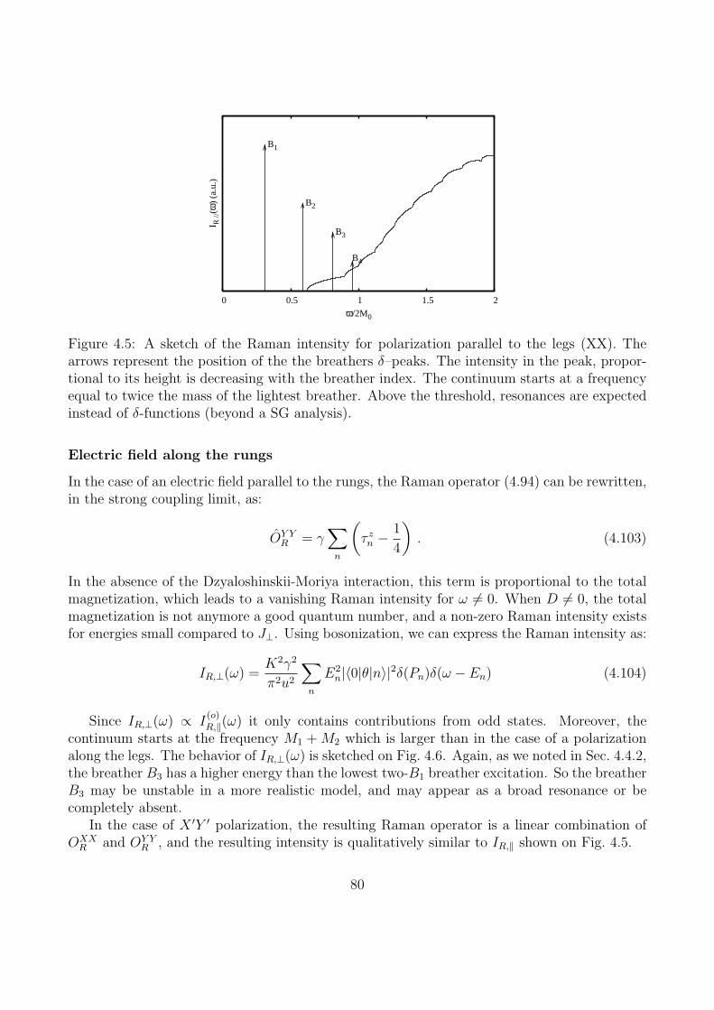
0 0.5 1 1.5 2
I R //
(ω)
(a.u
.)
ω/2M0
B1
B2
B3
B4
Figure 4.5: A sketch of the Raman intensity for polarization parallel to the legs (XX). Thearrows represent the position of the the breathers δ–peaks. The intensity in the peak, propor-tional to its height is decreasing with the breather index. The continuum starts at a frequencyequal to twice the mass of the lightest breather. Above the threshold, resonances are expectedinstead of δ-functions (beyond a SG analysis).
Electric field along the rungs
In the case of an electric field parallel to the rungs, the Raman operator (4.94) can be rewritten,in the strong coupling limit, as:
OY YR = γ
∑
n
(
τ zn − 1
4
)
. (4.103)
In the absence of the Dzyaloshinskii-Moriya interaction, this term is proportional to the totalmagnetization, which leads to a vanishing Raman intensity for ω 6= 0. When D 6= 0, the totalmagnetization is not anymore a good quantum number, and a non-zero Raman intensity existsfor energies small compared to J⊥. Using bosonization, we can express the Raman intensity as:
IR,⊥(ω) =K2γ2
π2u2
∑
n
E2n|〈0|θ|n〉|2δ(Pn)δ(ω − En) (4.104)
Since IR,⊥(ω) ∝ I(o)R,‖(ω) it only contains contributions from odd states. Moreover, the
continuum starts at the frequency M1 +M2 which is larger than in the case of a polarizationalong the legs. The behavior of IR,⊥(ω) is sketched on Fig. 4.6. Again, as we noted in Sec. 4.4.2,the breather B3 has a higher energy than the lowest two-B1 breather excitation. So the breatherB3 may be unstable in a more realistic model, and may appear as a broad resonance or becompletely absent.
In the case of X ′Y ′ polarization, the resulting Raman operator is a linear combination ofOXX
R and OY YR , and the resulting intensity is qualitatively similar to IR,‖ shown on Fig. 4.5.
80
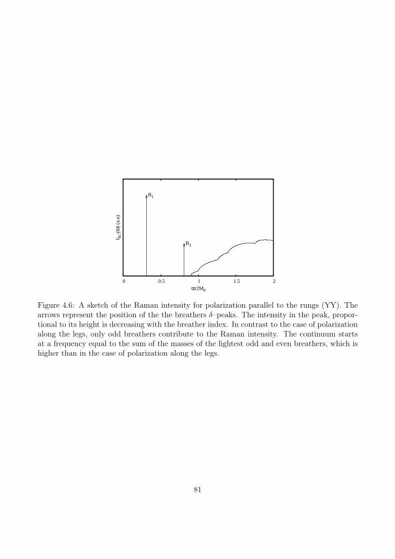
0 0.5 1 1.5 2
I R⊥
(ω)
(a.u
)
ω/2M0
B1
B3
Figure 4.6: A sketch of the Raman intensity for polarization parallel to the rungs (YY). Thearrows represent the position of the the breathers δ–peaks. The intensity in the peak, propor-tional to its height is decreasing with the breather index. In contrast to the case of polarizationalong the legs, only odd breathers contribute to the Raman intensity. The continuum startsat a frequency equal to the sum of the masses of the lightest odd and even breathers, which ishigher than in the case of polarization along the legs.
81
Chapter 5
the spin-Peierls transition
The present chapter is based on the article[227]
It is well known that one-dimensional metals on a deformable lattice are unstable[228]: adeformation of the lattice of wavevector 2kF creates a periodic potential that opens a gap at theFermi level turning the one-dimensional metal into a band insulator. In a mean-field theory,the gap can be shown to possess a BCS-like expression. Since we have seen that a XY spin-1/2chain could be mapped to one dimensional spinless fermions on a lattice, an XY spin-1/2 chainwill exhibit the same instability, with a lattice modulation of wavevector π/a (where a is thelattice spacing) in zero external field.[229, 230, 231] This instability is called the spin-Peierlsinstability. In the case of the XXZ chain, the Hamiltonian takes the form:
H = J∑
n
(1 + λ(un+1 − un))(SxnS
xn+1 + Sy
nSyn+1 +∆Sz
nSzn+1) +Hphonons, (5.1)
where un is the displacement of the n-th site, g is a spin-phonon coupling constant, ∆ = Jz/Jis the anisotropy. In the spin-Peierls phase, 〈un〉 = (−)nu. The presence of Jz 6= 0, the spin-phonon is renormalized by Jz. A mean-field theory taking into account such renormalizationwas developed in 1979.[232] The bosonized theory takes the form:
H =
∫
dx
2π
[
uK(πΠ)2 +u
K(∂xφ)
2]
− 2gδ
(2πα)2cos
√2φ+
k
2δ2, (5.2)
where the dimensionless dimerization parameter δ = 2λu and k depends on the elastic con-stants of the lattice. The amplitude g is coming from the bosonized form of the dimerizationoperator (1.68) and is a non-universal parameter, not known in general. The notation in (5.2)is chosen so that the case with SU(2) symmetry corresponds to K = 1 while the case ∆ = 0corresponds to K = 2.
For δ 6= 0, the cost in elastic energy is kδ2/2, while the energy gained from the openingof a spin gap is obtained from scaling as: ∼ δδK/(4−K) = δ4/(4−K). The case K = 2 is themarginal case (where the energy gain actually contains a logarithmic factor). For K > 2 (i.e. Jz < 0), the energy gained from the opening of the spin gap is insufficient to compensatethe cost in elastic energy, while for K < 2 (i. e. Jz < 0) the energy gained makes it always
82
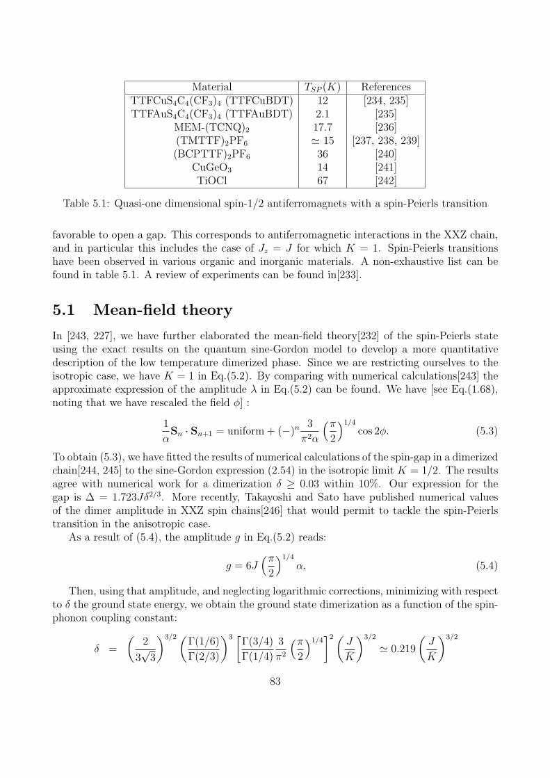
Material TSP (K) ReferencesTTFCuS4C4(CF3)4 (TTFCuBDT) 12 [234, 235]TTFAuS4C4(CF3)4 (TTFAuBDT) 2.1 [235]
MEM-(TCNQ)2 17.7 [236](TMTTF)2PF6 ≃ 15 [237, 238, 239](BCPTTF)2PF6 36 [240]
CuGeO3 14 [241]TiOCl 67 [242]
Table 5.1: Quasi-one dimensional spin-1/2 antiferromagnets with a spin-Peierls transition
favorable to open a gap. This corresponds to antiferromagnetic interactions in the XXZ chain,and in particular this includes the case of Jz = J for which K = 1. Spin-Peierls transitionshave been observed in various organic and inorganic materials. A non-exhaustive list can befound in table 5.1. A review of experiments can be found in[233].
5.1 Mean-field theory
In [243, 227], we have further elaborated the mean-field theory[232] of the spin-Peierls stateusing the exact results on the quantum sine-Gordon model to develop a more quantitativedescription of the low temperature dimerized phase. Since we are restricting ourselves to theisotropic case, we have K = 1 in Eq.(5.2). By comparing with numerical calculations[243] theapproximate expression of the amplitude λ in Eq.(5.2) can be found. We have [see Eq.(1.68),noting that we have rescaled the field φ] :
1
αSn · Sn+1 = uniform + (−)n
3
π2α
(π
2
)1/4
cos 2φ. (5.3)
To obtain (5.3), we have fitted the results of numerical calculations of the spin-gap in a dimerizedchain[244, 245] to the sine-Gordon expression (2.54) in the isotropic limit K = 1/2. The resultsagree with numerical work for a dimerization δ ≥ 0.03 within 10%. Our expression for thegap is ∆ = 1.723Jδ2/3. More recently, Takayoshi and Sato have published numerical valuesof the dimer amplitude in XXZ spin chains[246] that would permit to tackle the spin-Peierlstransition in the anisotropic case.
As a result of (5.4), the amplitude g in Eq.(5.2) reads:
g = 6J(π
2
)1/4
α, (5.4)
Then, using that amplitude, and neglecting logarithmic corrections, minimizing with respectto δ the ground state energy, we obtain the ground state dimerization as a function of the spin-phonon coupling constant:
δ =
(
2
3√3
)3/2(Γ(1/6)
Γ(2/3)
)3 [Γ(3/4)
Γ(1/4)
3
π2
(π
2
)1/4]2(
J
K
)3/2
≃ 0.219
(
J
K
)3/2
83
∆ =2√π
3√3
(
Γ(1/6)
Γ(2/3)
)3 [Γ(3/4)
Γ(1/4)
3
π2
(π
2
)1/4]2J2
K≃ 0.627
J2
K, (5.5)
where K = kα.Using high-temperature perturbation theory as in 4.3, we obtain the approximate expression
of the free energy:
Fs(T, δ) = − π
6uT 2 − a
4
(
2gδ
(2πa)2
)2π2
Γ(3/4)4T
= − π
6uT 2 − 9J2δ2
4π2Γ(34)4aT
(π
2
)1/2
, (5.6)
from which we deduce:
TSP =9
2π2Γ(3/4)4
(π
2
)1/2 J2
K= 0.25342
J2
K(5.7)
Compared with the original mean-field theory[232], the exponents are of course recovered, butthe amplitudes are also determined. Moreover, for 0 < T < TSP , it is possible to use the resultsof [86, 87, 88] to calculate at any temperature the Free energy of the sine-Gordon model. Usingδ as a parameter, we can minimize the sum of the sine Gordon free energy and the elasticenergy. This allows us to obtain the temperature dependence of δ. In turn, knowing thatquantity allows the quantitative determination of the free energy.
The sine-Gordon model with K = 1/2 and cos 2φ is mapped to the form (2.1) by therescaling φ →
√2φ and K → K/2. Using the Eq.(2.56) with K = 1/4 we note that there
are two breathers, a light one of mass M1 = M and a heavy one of mass M2 = M√3. The
light breather has the same mass as the solitons, and possesses a spin Sz = 0 while the solitonand antisoliton possess the spins Sz = ±1. Together, they form a massive spin triplet[81, 82]with the heavy breather forming a spin singlet. The sine-Gordon model is at a reflectionlesspoint, and as a consequence of the SU(2) symmetry, there are only three different S-matrixamplitudes corresponding to triplet-triplet collisions (S11), singlet-triplet collisions (S12) andsinglet-singlet collisions (S22).
Knowing the masses of the excitations, we can thus use (2.76) to determine the free energya for given dimerization.
We have obtained the following equations[227]:
Fs(T, δ) = − T
2πu
∫ ∞
−∞dθ∆cosh θ
[
3 ln(1 + e−ǫ1(θ)/T ) +√3 ln(1 + e−ǫ2(θ)/T )
]
− u
a2tan
π
6
M2
4(5.8)
where the pseudoenergies are solutions of the integral equations:
ǫ1(θ) = ∆cosh θ +3T
2π
∫ ∞
−∞dθ′K11(θ − θ′) ln(1 + e−ǫ1(θ′)/T ) +
T
2π
∫ ∞
−∞dθ′K12(θ − θ′) ln(1 + e−ǫ2(θ′)/T ),
ǫ2(θ) = ∆√3 cosh θ +
3T
2π
∫ ∞
−∞dθ′K12(θ − θ′) ln(1 + e−ǫ1(θ′)/T ) +
T
2π
∫ ∞
−∞dθ′K22(θ − θ′) ln(1 + e−ǫ2(θ′)/T ),
(5.9)
84
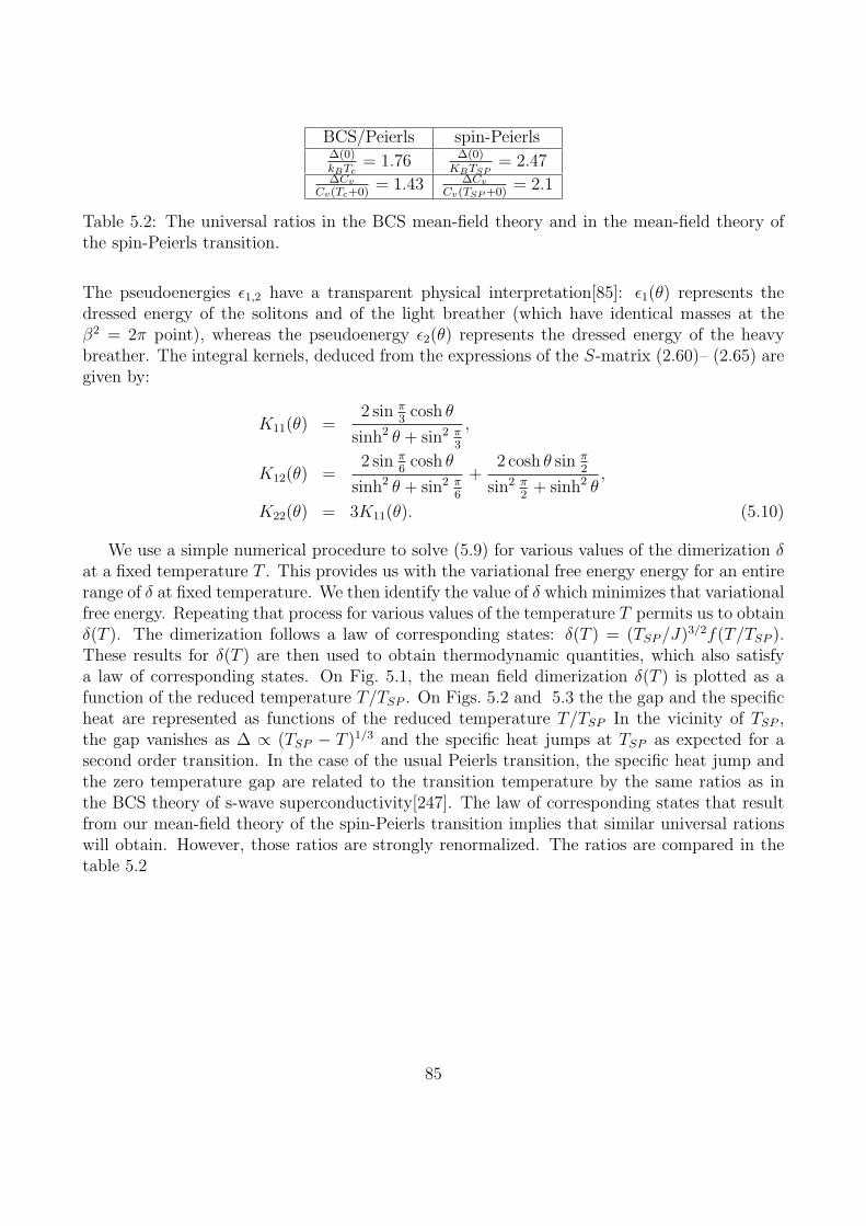
BCS/Peierls spin-Peierls∆(0)kBTc
= 1.76 ∆(0)KBTSP
= 2.47∆Cv
Cv(Tc+0)= 1.43 ∆Cv
Cv(TSP+0)= 2.1
Table 5.2: The universal ratios in the BCS mean-field theory and in the mean-field theory ofthe spin-Peierls transition.
The pseudoenergies ǫ1,2 have a transparent physical interpretation[85]: ǫ1(θ) represents thedressed energy of the solitons and of the light breather (which have identical masses at theβ2 = 2π point), whereas the pseudoenergy ǫ2(θ) represents the dressed energy of the heavybreather. The integral kernels, deduced from the expressions of the S-matrix (2.60)– (2.65) aregiven by:
K11(θ) =2 sin π
3cosh θ
sinh2 θ + sin2 π3
,
K12(θ) =2 sin π
6cosh θ
sinh2 θ + sin2 π6
+2 cosh θ sin π
2
sin2 π2+ sinh2 θ
,
K22(θ) = 3K11(θ). (5.10)
We use a simple numerical procedure to solve (5.9) for various values of the dimerization δat a fixed temperature T . This provides us with the variational free energy energy for an entirerange of δ at fixed temperature. We then identify the value of δ which minimizes that variationalfree energy. Repeating that process for various values of the temperature T permits us to obtainδ(T ). The dimerization follows a law of corresponding states: δ(T ) = (TSP/J)
3/2f(T/TSP ).These results for δ(T ) are then used to obtain thermodynamic quantities, which also satisfya law of corresponding states. On Fig. 5.1, the mean field dimerization δ(T ) is plotted as afunction of the reduced temperature T/TSP . On Figs. 5.2 and 5.3 the the gap and the specificheat are represented as functions of the reduced temperature T/TSP In the vicinity of TSP ,the gap vanishes as ∆ ∝ (TSP − T )1/3 and the specific heat jumps at TSP as expected for asecond order transition. In the case of the usual Peierls transition, the specific heat jump andthe zero temperature gap are related to the transition temperature by the same ratios as inthe BCS theory of s-wave superconductivity[247]. The law of corresponding states that resultfrom our mean-field theory of the spin-Peierls transition implies that similar universal rationswill obtain. However, those ratios are strongly renormalized. The ratios are compared in thetable 5.2
85
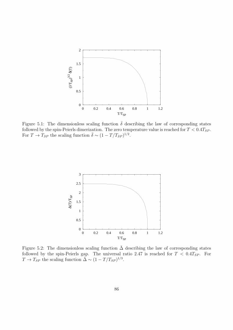
0
0.5
1
1.5
2
0 0.2 0.4 0.6 0.8 1 1.2
(J/T
SP)3/
2 δ(T
)
T/TSP
Figure 5.1: The dimensionless scaling function δ describing the law of corresponding statesfollowed by the spin-Peierls dimerization. The zero temperature value is reached for T < 0.4TSP .For T → TSP the scaling function δ ∼ (1− T/TSP )
1/2.
0
0.5
1
1.5
2
2.5
3
0 0.2 0.4 0.6 0.8 1 1.2
∆(T
)/T
SP
T/TSP
Figure 5.2: The dimensionless scaling function ∆ describing the law of corresponding statesfollowed by the spin-Peierls gap. The universal ratio 2.47 is reached for T < 0.4TSP . ForT → TSP the scaling function ∆ ∼ (1− T/TSP )
1/3.
86
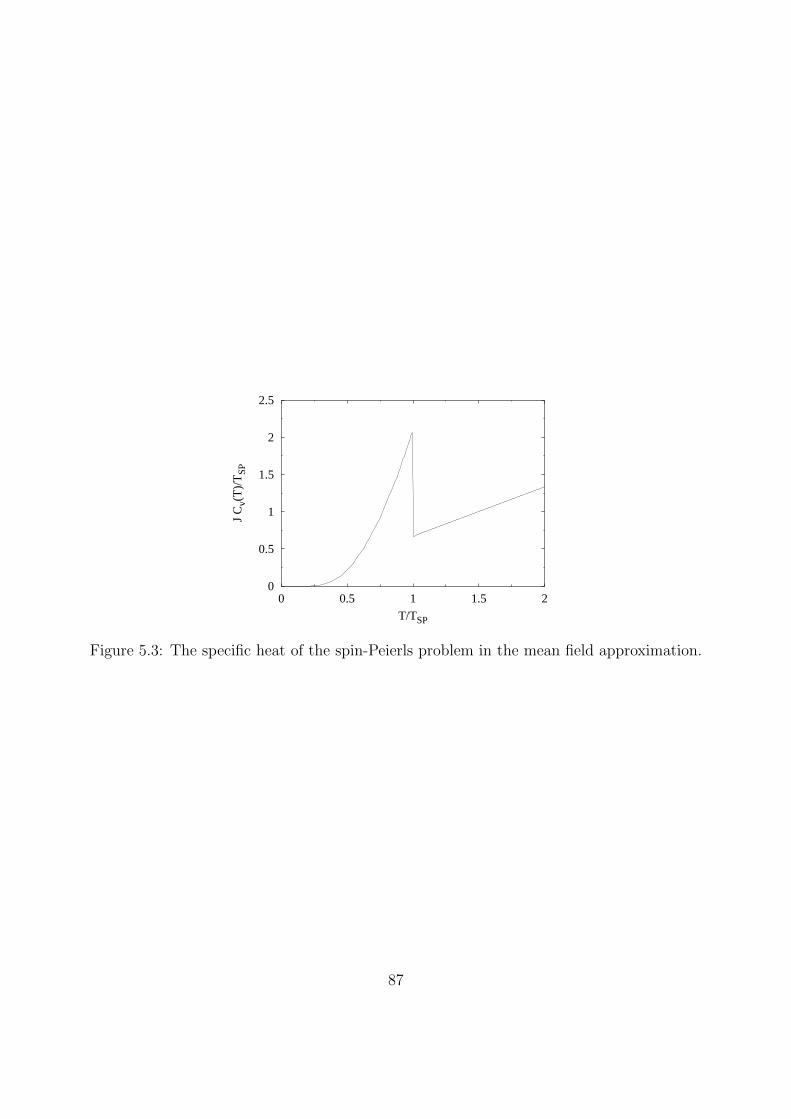
0
0.5
1
1.5
2
2.5
0 0.5 1 1.5 2
J C
v(T
)/T
SP
T/TSP
Figure 5.3: The specific heat of the spin-Peierls problem in the mean field approximation.
87
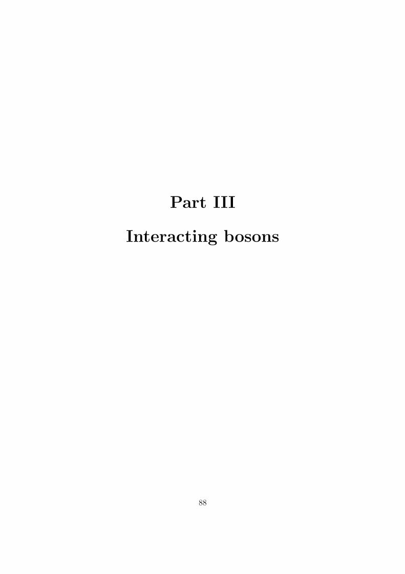
Part III
Interacting bosons
88
Chapter 6
Dipolar bosons
The present chapter is based on the articles[248, 249, 250, 251].
6.1 qualitative considerations
In trapped gases, the atoms are neutral, and their interactions are of the Van der Waals type.A phenomenological description of the interaction is obtained by using a contact interactionwhich reproduces the scattering cross section,
V (r) =4πa
mδ(r). (6.1)
In the case of gases trapped in a quasi-one dimensional geometry, the transverse degrees offreedom are frozen, and the interaction becomes a one-dimensional δ interaction. One obtainsthe Lieb-Liniger model[29] which is integrable. Experiments with trapped gases has beensucessfully interpreted within that framework[144, 142, 140]. Recently, atomic gases carrying apermanent magnetic dipolar moment have been trapped[252, 253] If those gases are polarizedby an applied magnetic field, a dipole-dipole interaction
Vdip.(r) =µ0
4π
m1 ·m2 − 3(m1 · r)(m1 · r)|r|3 , (6.2)
where m is the magnetic moment of an atom, and r = r/|r| is present. Moreover, moleculeswith permanent electric dipoles have been also trapped (but not cooled to degeneracy) andin these systems electric dipole forces are also present. When the dipoles are polarized in adirection orthogonal to the axis, the forces are repulsive, and vary as C/r3.
In one-dimension, dipolar interactions are short range forces, with∫∞a
|Vdip.(r)|dr < ∞,where a is a short distance cutoff. The Mermin-Wagner-Hohenberg theorem ensures that theycannot induce a crystalline order[16, 17, 18] and a Tomonaga-Luttinger liquid is still expected.However, for short distances, in one dimension, the dipolar forces are strongly repulsive. Indeed,if we consider a two-body Schrodinger equation,
H = − 1
2m∂2xψ +
C
|x|3ψ = Eψ, (6.3)
89
where x is the relative coordinate, a semiclassical WKB approximation gives a wavefunctionψ(x) varying as:
ψ(x) ∼ 1√mC
e−2
√
mC|x| , (6.4)
and vanishing when the particles are coming in contact. As a result, in a dilute gas of dipo-lar particles, where three-body interactions are infrequent, one expects that the many-bodywavefunction vanishes anytime two particles are at the same point. Such a condition is alsosatisfied in a fermionic gas. However, the wavefunction of a fermion gas is antisymmetric underpermutation of particles, while the wavefunction of a Bose gas is symmetric under particlepermutation. This difference can be corrected by multiplying the fermion wavefunction by afactor:
∏
i<j
sign(xi − xj) = sign
[
∏
i<j
(xi − xj)
]
, (6.5)
indeed, the expression in the right hand-side of (6.5) is the sign of a Vandermonde determinant(the columns of which are successive powers of the coordinates of the particles) which is changingsign under permutation of the particle coordinates. Multiplying the factor (6.5) by a fermionicwavefunction gives a function that does not change sign under permutation of particles butvanishes every time two particles are at the same point. This process in in fact[254] a firstquantized version of the Jordan-Wigner transformation (1.57). Since in a dilute dipolar gasinteractions beyond two body can be neglected, one can take as the fermionic wavefunctiona Slater determinant of plane waves. This leads us to expect that the dilute gas of bosonicparticles has the same thermodynamics as a free fermionic gas, with an energy per unit lengthvarying as e(n0) ∝ n3
0. In the opposite limit of high density, if we were dealing with a classicalgas, the repulsion between the particles would give us a one dimensional crystal. In such acrystal, the energy per unit length would be:
e(n0) = Cζ(3)n40, (6.6)
where n0 is the number of particles per unit length, and would dominate the kinetic energyfrom zero point motion, ∝ n3
0. Since the system is in the Tomonaga-Luttinger liquid state, wecan use (6.6) to estimate the particle velocity and Tomonaga-Luttinger exponent. By Galileaninvariance (1.80),
uK =πn0
M, (6.7)
and by the compressibility relation (1.76), giving
K =π
√
12ζ(3)Mn0
. (6.8)
From these qualitative considerations, we expect that for low density K → 1 and for highdensity K → 0. This is to be contrasted with the behavior of the Luttinger exponent in theLieb-Liniger gas, where K → +∞ for high density, and K → 1 for low density. The dipolar iscovering a range of Tomonaga-Luttinger exponent complementary to that of the Lieb-Linigergas.
90
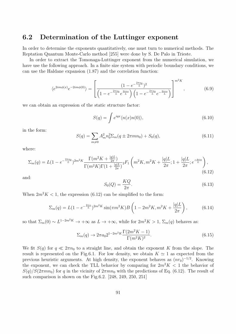
6.2 Determination of the Luttinger exponent
In order to determine the exponents quantitatively, one must turn to numerical methods. TheReptation Quantum Monte-Carlo method [255] were done by S. De Palo in Trieste.
In order to extract the Tomonaga-Luttinger exponent from the numerical simulation, wehave use the following approach. In a finite size system with periodic boundary conditions, wecan use the Haldane expansion (1.87) and the correlation function:
〈e2imφ(x)e−2imφ(0)〉 =
(1− e−2πa0L )2
(
1− e−2πa0L e
2iπxL
)(
1− e−2πa0L e−
2iπxL
)
m2K
, (6.9)
we can obtain an expression of the static structure factor:
S(q) =
∫
eiqx〈n(x)n(0)〉, (6.10)
in the form:S(q) =
∑
m 6=0
A2mn
20Σm(q ± 2πmn0) + S0(q), (6.11)
where:
Σm(q) = L(1− e−2πa0L )2m
2K Γ(m2K + |q|L2π
)
Γ(m2K)Γ(1 + |q|L2π
)2F1
(
m2K,m2K +|q|L2π
; 1 +|q|L2π
; e−4πα
L
)
,
(6.12)and:
S0(Q) =KQ
2π. (6.13)
When 2m2K < 1, the expression (6.12) can be simplified to the form:
Σm(q) = L(1− e−2παL )2m
2K sin(πm2K)B
(
1− 2m2K,m2K +|q|L2π
)
, (6.14)
so that Σm(0) ∼ L1−2m2K → +∞ as L→ +∞, while for 2m2K > 1, Σm(q) behaves as:
Σm(q) → 2πa021−2m2K Γ(2m2K − 1)
Γ(m2K)2. (6.15)
We fit S(q) for q ≪ 2πn0 to a straight line, and obtain the exponent K from the slope. Theresult is represented on the Fig.6.1. For low density, we obtain K ≃ 1 as expected from theprevious heuristic arguments. At high density, the exponent behaves as (nr0)
−1/2. Knowingthe exponent, we can check the TLL behavior by comparing for 2m2K < 1 the behavior ofS(q)/S(2πmn0) for q in the vicinity of 2πmn0 with the predictions of Eq. (6.12). The result ofsuch comparison is shown on the Fig.6.2. [248, 249, 250, 251]
91
S(k
)
k/n
0.01
0.1
1
10
100
0.01 0.1 1 10 100 1000
K
nr0
Figure 6.1: The Tomonaga-Luttinger exponent of the one-dimensional gas of dipoles as afunction of density. The squares are the numerically computed exponent, the dotted line is thehard-core boson exponent, the dashed line the high density limit. In the inset, the structurefactor for different values of the density has been represented. The linear slope at the origindirectly gives the Tomonaga-Luttinger exponent. From [248]
0.001
0.01
0.1
1
-4 -3 -2 -1 0 1 2 3 4
S(k
)/S
(2π)
N(k/n -2π)/40
N=40N=60N=80
N=100LL
Figure 6.2: Scaling of the structure factor in the vicinity of the peak k = 2πρ0 at fixed densityand for an increasing system size. The solid line is the prediction from the Tomonaga-Luttingerliquid theory. From [248]
92
Chapter 7
Bosonic ladders under field
The present chapter is based on the article [256].
We consider two one-dimensional bosonic chains coupled by interchain repulsion and inter-chain hopping. Those systems can be realized either by coupling Josephson junctions or bycoupling two one-dimensional trapped atomic gases. The Hamiltonian of coupled Josephsonjunctions reads[257, 258, 259]
H = −∑
n,p
[
J‖ cos(θn,p − θn+1,p) +e2
2CN2
n,p − eVgNn,p
]
−∑
n
[
J⊥ cos(θn,1 − cos θn,2) +e2
C⊥Nn,1Nn,2
]
, (7.1)
where J‖, J⊥ are the longitudinal and transverse Josephson couplings, C is the capacity to theground, and Vg is the gate voltage. From the Eqs. (1.93) and (1.87), it is easily seen thatthose systems have the same Hamiltonian (4.10) as two-leg spin ladders. The phase diagramof the spin ladders translate directly into a phase diagram for the boson ladders. However,in Josephson ladders, the Cooper pairs are charged, and are sensitive to an applied externalmagnetic field. To consider the effect of an external magnetic field, we must first remark that(7.1) is not gauge invariant. Indeed, under a gauge transformation of the vector potentialA→ A+∇χ, the Cooper pair creation operator transforms as:
eiθn,p → eiθn,p+2eχn,p , (7.2)
so that in order to obtain a gauge invariant expression we have to make the Peierls substitution:
ei(θn−θm) → ei(θn−θm)−2e∫m
nAdr, (7.3)
We can choose a gauge with the vector potential A = −Byex along the chains. In that gauge,the longitudinal Josephson couplings become:
J‖ cos (θn,p − θn+1,p − eB(p− 1/2)ba) , (7.4)
where a is the length of a junction along the chain, and b is the length of a rung junction and thetransverse couplings are unchanged. In the case of coupled one-dimensional gases, it is possible
93
to create artificial gauge fields that simulate the effect of a uniform magnetic field.[260, 261, 262]After bosonization, the Hamiltonian becomes[263]
H = Hs +Ha
Ha =
∫
dx
2π
[
uaKa(πΠa − e∗Aa)2 +
uaKa
(∂xφa)2
]
− J⊥πa
∫
dx cos(√2θa)
+2V a
(2πa)2
∫
dx cos√8φa, (7.5)
with V ∼ e2/C⊥ and the currents are:
ja = uKe∗√2(Πν −
e∗
πAν) (7.6)
j⊥ =e∗J⊥πa
sin(√2θa) (7.7)
The Hamiltonian (7.5) also describes a two-leg spin ladder having different uniform Dzyaloshinskii-Moriya interactions on the two legs.
With a weak external field, the Hamiltonian Ha remains gapped with 〈ja〉 = −uK (e∗)2Φπa
and 〈j⊥〉 = 0. There is only a current circulating along the edge of the system, with no currentin the bulk of the ladder. That low field phase can be identified with a Meissner phase[258].Under a stronger field, a commensurate-incommensurate transition as discussed in Sec.4.3 canbe obtained. There are however two differences with the case of the ladder in applied field.The obvious first one is that now the field θa is coupled to the applied magnetic field insteadof the field φs. The second, and more important difference, is that the field cos
√8φa is also
present in Ha. Since at the transition K∗a = 1/2, that field is relevant, the commensurate-
incommensurate transition is avoided[264] and the system remains gapped across the transition.In the magnetized phase, the system is showing power-law density wave correlations withexponential decay of the bosonic correlation functions 〈eiθn,pe−iθm,p〉.
For sufficiently large field, we can have K∗a(h) > 1 and cos
√8φa again irrelevant. The
spectrum of Ha is then gapless and both density wave and bosonic correlations decay as power-laws. The gapful regime and the gapless regime are separated by a Kosterlitz-Thouless phasetransition.
In the presence of a stronger flux, close to a rational number p/q of quantum of flux perplaquette e∗Φ = 2π p
q+δΦ, with the denominator q not too large and δΦ ≪ 2π p
q, the gauge with
the vector potential along the legs of the ladder is not convenient for perturbative bosonizationas it would give an very large field. The most convenient gauge choice is instead A⊥(n) =n(2πe∗p)/q and Aa = (δΦ)/(a
√2). With such a gauge choice, the interchain Josephson coupling
is of the form:J⊥∑
n
cos(θn,1 − θn,2 − A⊥(n)), (7.8)
which is in general an oscillating term and gives a vanishing contribution to the Hamiltonianin bosonization. However, perturbation theory to order q will give a term:
(J⊥)q/Jq−1
‖
∑
n
cos q(θn,1 − θn,2), (7.9)
94
which is not oscillating since qA⊥(n) is an integer multiple of 2π. After bosonization, we obtaina Hamiltonian of the form:
Ha =
∫
dx
2π
[
uaKa(πΠa − e∗Aa)2 +
uaKa
(∂xφa)2
]
− Jq⊥
πJq−1‖ a
∫
dx cos(q√2θa)
+2V a
(2πa)2
∫
dx cos√8φa, (7.10)
which, when 4Ka > q2 can present a gapful phase for small δΦ and a gapless phase for larger δΦ.We note that for q ≥ 2, the cos
√8φa term is irrelevant, and will not modify the commensurate
incommensurate transition in contrast to the zero-flux case. In the gapful phase, the gappedexcitations are vortices carrying a fractional flux 2π/q. The gauge transformation makes thetransverse current j⊥ = J⊥ sin(
√2θa − A⊥(n)) a spatially modulated quantity. In the gapful
phase, 〈j⊥〉(x) becomes a periodic function of x, while the longitudinal current 〈j‖〉 = 0.Returning to the original gauge, this indicates that θn,1 − θn,2 is growing linearly with n i.
e. that a commensurate vortex lattice is formed. When δΦ is such that the system is in theincommensurate phase, 〈j⊥(x)〉 = 0 while 〈j‖〉 ∝ δΦ. That phase can be seen as a Luttingerliquid of vortices (carrying the fractional flux 2π/q). This leads us to conjecture the followingform of the vortex density:
ρV (x) =1
π√2∂xθa +
m=∞∑
m=−∞
Cm
πaeim[2πρV x+
√2(θa−〈θa〉)] (7.11)
When the density of vortices is p/q, the potential energy term (7.9) can be interpreted as thecoupling of the vortex density to a pinning potential of period q lattice spacings.
In the classical case [265], a vortex lattice phase is obtained each time the flux per plaquettein a rational multiple of the quantum of flux, leading to a devil’s staircase structure in thebehavior of the magnetization. Here, the quantum fluctuations wipe out the large fractions forwhich q2 > 4Ka, so only some plateaux remain as shown on Fig. 7.1.
It is also possible to use the fermionization approach to calculate the behavior of the currentin the ladder in the vicinity of the commensurate-incommensurate transition for q > 1. Wefind that the current behaves as:
〈ja〉 =u(e∗)2
2πa(√
Φ2 − Φ2cθ(Φ
2 − Φ2c)− Φ) (7.12)
For Φ < Φc, the current is linear in flux, producing a one-dimensional analog of the Meissnereffect. When Φ > Φc, vortices appear in the ladder, and the applied flux is only partiallyscreened.
95
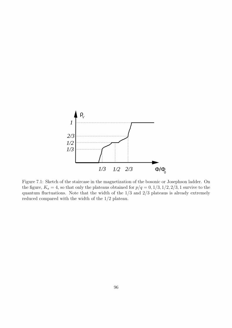
1/2
V
1/3
1
2/3
1/21/3 2/3 Φ/Φ0
ρ
Figure 7.1: Sketch of the staircase in the magnetization of the bosonic or Josephson ladder. Onthe figure, Ka = 4, so that only the plateaus obtained for p/q = 0, 1/3, 1/2, 2/3, 1 survive to thequantum fluctuations. Note that the width of the 1/3 and 2/3 plateaus is already extremelyreduced compared with the width of the 1/2 plateau.
96
Chapter 8
Disordered bosons
The present chapter is based on the articles [266, 267].
8.1 The Aubry-Andre transition
The Aubry-Andre transition was predicted in tight-binding chains with an on-site quasiperiodicpotential.[268] The Aubry-Andre Hamiltonian reads:
H = −t∑
n
(a†nan+1 + a†n+1an) + ∆∑
n
cos(2πQn)a†nan, (8.1)
where Q is an irrational number so that the potential in (8.1) is not periodic. Going to Fourierspace,
an =1√N
∑
n
akeikn, (8.2)
we rewrite the Hamiltonian (8.1) as:
H =∑
k
[
−2t cos(k)a†kak +∆eiφ
2a†kak−2πQ +
∆e−iφ
2a†kak+2πQ
]
(8.3)
We note that the Hamiltonian (8.3) is of a form similar to (8.1), the sites being the momen-tas 2πnQ, the kinetic energy −2t cos(2πnQ) being the on-site energy, and the hopping being∆/2.Here, the irrationality of Q plays a crucial role. The set of numbers nQ+m with n,m ∈ Z
is dense in the set of real numbers allowing us to approximate any momentum k as 2πnQ forsome n. The mapping of the Hamiltonian (8.1) on the Hamiltonian (8.3) is a duality transfor-mation, that exchanges ∆ with 2t. For small ∆/(2t), the eigenstates of (8.1) are extended inreal space, and the eigenstates of (8.3) are localized. Vice-versa, for large ∆/(2t), the eigen-states of (8.1) are localized, while those of (8.3) are extended. Thus, a transition from extendedto localized eigenstates is expected in the Aubry-Andre model at the self-dual point ∆ = 2t.Under that hypothesis, the localization length in the phase ∆ > 2t can be obtained from the
97
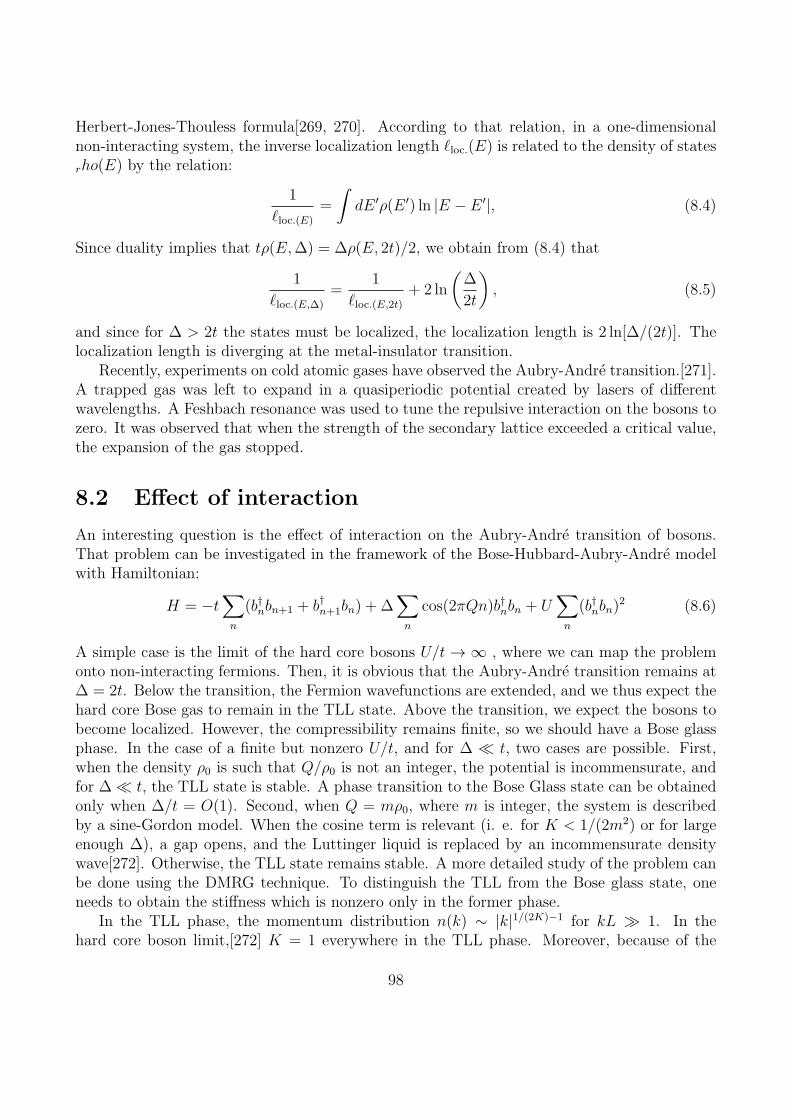
Herbert-Jones-Thouless formula[269, 270]. According to that relation, in a one-dimensionalnon-interacting system, the inverse localization length ℓloc.(E) is related to the density of states
rho(E) by the relation:
1
ℓloc.(E)
=
∫
dE ′ρ(E ′) ln |E − E ′|, (8.4)
Since duality implies that tρ(E,∆) = ∆ρ(E, 2t)/2, we obtain from (8.4) that
1
ℓloc.(E,∆)
=1
ℓloc.(E,2t)
+ 2 ln
(
∆
2t
)
, (8.5)
and since for ∆ > 2t the states must be localized, the localization length is 2 ln[∆/(2t)]. Thelocalization length is diverging at the metal-insulator transition.
Recently, experiments on cold atomic gases have observed the Aubry-Andre transition.[271].A trapped gas was left to expand in a quasiperiodic potential created by lasers of differentwavelengths. A Feshbach resonance was used to tune the repulsive interaction on the bosons tozero. It was observed that when the strength of the secondary lattice exceeded a critical value,the expansion of the gas stopped.
8.2 Effect of interaction
An interesting question is the effect of interaction on the Aubry-Andre transition of bosons.That problem can be investigated in the framework of the Bose-Hubbard-Aubry-Andre modelwith Hamiltonian:
H = −t∑
n
(b†nbn+1 + b†n+1bn) + ∆∑
n
cos(2πQn)b†nbn + U∑
n
(b†nbn)2 (8.6)
A simple case is the limit of the hard core bosons U/t → ∞ , where we can map the problemonto non-interacting fermions. Then, it is obvious that the Aubry-Andre transition remains at∆ = 2t. Below the transition, the Fermion wavefunctions are extended, and we thus expect thehard core Bose gas to remain in the TLL state. Above the transition, we expect the bosons tobecome localized. However, the compressibility remains finite, so we should have a Bose glassphase. In the case of a finite but nonzero U/t, and for ∆ ≪ t, two cases are possible. First,when the density ρ0 is such that Q/ρ0 is not an integer, the potential is incommensurate, andfor ∆ ≪ t, the TLL state is stable. A phase transition to the Bose Glass state can be obtainedonly when ∆/t = O(1). Second, when Q = mρ0, where m is integer, the system is describedby a sine-Gordon model. When the cosine term is relevant (i. e. for K < 1/(2m2) or for largeenough ∆), a gap opens, and the Luttinger liquid is replaced by an incommensurate densitywave[272]. Otherwise, the TLL state remains stable. A more detailed study of the problem canbe done using the DMRG technique. To distinguish the TLL from the Bose glass state, oneneeds to obtain the stiffness which is nonzero only in the former phase.
In the TLL phase, the momentum distribution n(k) ∼ |k|1/(2K)−1 for kL ≫ 1. In thehard core boson limit,[272] K = 1 everywhere in the TLL phase. Moreover, because of the
98
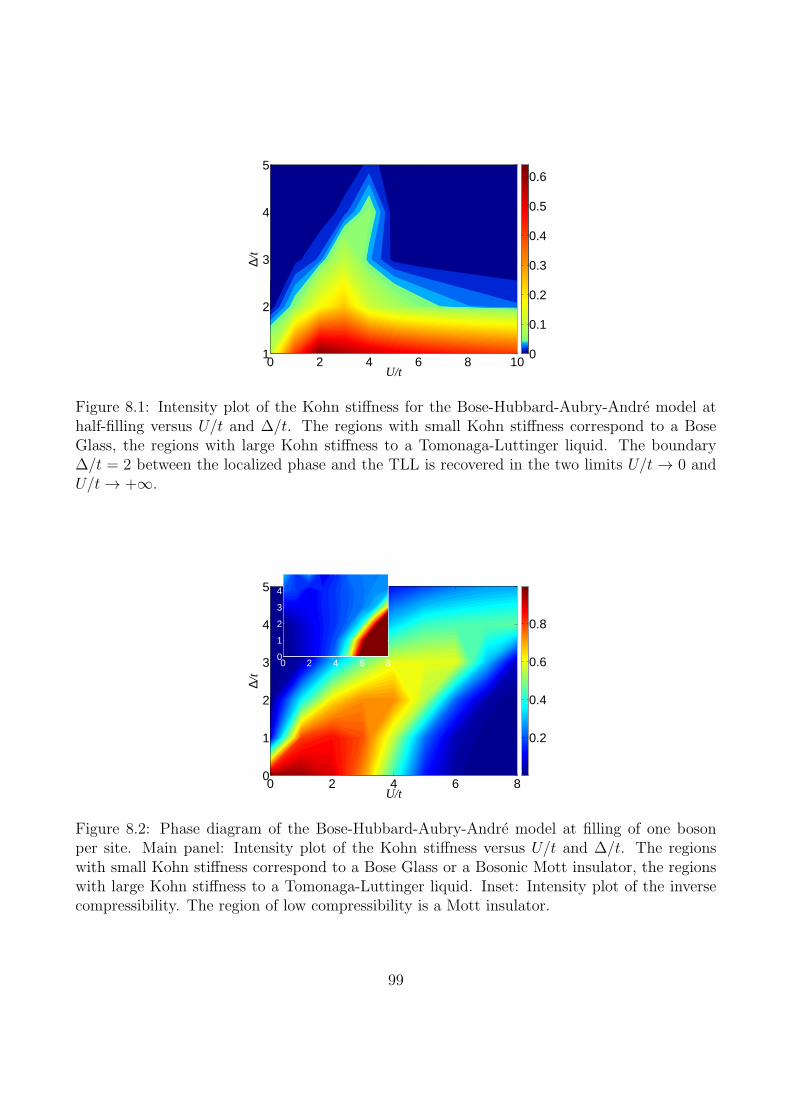
U/t
∆/t
0 2 4 6 8 101
2
3
4
5
0
0.1
0.2
0.3
0.4
0.5
0.6
Figure 8.1: Intensity plot of the Kohn stiffness for the Bose-Hubbard-Aubry-Andre model athalf-filling versus U/t and ∆/t. The regions with small Kohn stiffness correspond to a BoseGlass, the regions with large Kohn stiffness to a Tomonaga-Luttinger liquid. The boundary∆/t = 2 between the localized phase and the TLL is recovered in the two limits U/t → 0 andU/t→ +∞.
U/t
∆/t
0 2 4 6 80
1
2
3
4
5
0.2
0.4
0.6
0.8
0 2 4 6 80
1
2
3
4
5
Figure 8.2: Phase diagram of the Bose-Hubbard-Aubry-Andre model at filling of one bosonper site. Main panel: Intensity plot of the Kohn stiffness versus U/t and ∆/t. The regionswith small Kohn stiffness correspond to a Bose Glass or a Bosonic Mott insulator, the regionswith large Kohn stiffness to a Tomonaga-Luttinger liquid. Inset: Intensity plot of the inversecompressibility. The region of low compressibility is a Mott insulator.
99
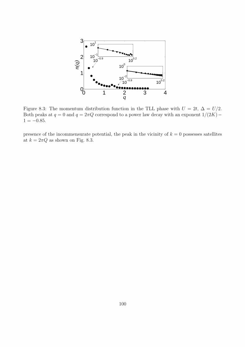
0 1 2 3 40
1
2
3
q
n(q
) 10−0.9
100.210
−1
101
10−0.9
100.210
−2
100
Figure 8.3: The momentum distribution function in the TLL phase with U = 2t, ∆ = U/2.Both peaks at q = 0 and q = 2πQ correspond to a power law decay with an exponent 1/(2K)−1 = −0.85.
presence of the incommensurate potential, the peak in the vicinity of k = 0 possesses satellitesat k = 2πQ as shown on Fig. 8.3.
100
Bibliography
[1] L. D. Landau, Sov. Phys. JETP 3, 920 (1957).
[2] L. D. Landau, Sov. Phys. JETP 5, 101 (1957).
[3] L. D. Landau, Sov. Phys. JETP 8, 70 (1958).
[4] P. Nozieres, Theory of Interacting Fermi Systems, Benjamin, New York, 1961.
[5] A. A. Abrikosov, L. P. Gorkov, and I. E. Dzyaloshinski, Methods of Quantum Field
Theory in Statistical Physics, Dover, New York, 1963.
[6] J. Solyom, Adv. Phys. 28, 209 (1979).
[7] V. J. Emery, Theory of the one-dimensional electron gas, in Highly conducting one-
dimensional solids, edited by J. T. Devreese, R. P. Evrard, and V. E. van Doren, page247, New York and London, 1979, Plenum Press.
[8] S. Tomonaga, Prog. Theor. Phys. 5, 544 (1950).
[9] J. M. Luttinger, J. Math. Phys. 4, 1154 (1963).
[10] F. D. M. Haldane, J. Phys. C 14, 2585 (1981).
[11] L. D. Landau and E. M. Lifshitz, Theory of Elasticity, Pergamon Press, New York, 1959.
[12] D. C. Mattis and E. H. Lieb, J. Math. Phys. 6, 304 (1965).
[13] A. Luther and I. Peschel, Phys. Rev. B 9, 2911 (1974).
[14] D. Orgad, Phil. Mag. B 81, 377 (2001).
[15] A. E. Mattson, S. Eggert, and H. Johannesson, Phys. Rev. B 56, 15615 (1997).
[16] N. D. Mermin and H. Wagner, Phys. Rev. Lett. 17, 1133 (1967).
[17] N. D. Mermin, Phys. Rev. 176, 250 (1968).
[18] P. C. Hohenberg, Phys. Rev. 158, 383 (1967).
101
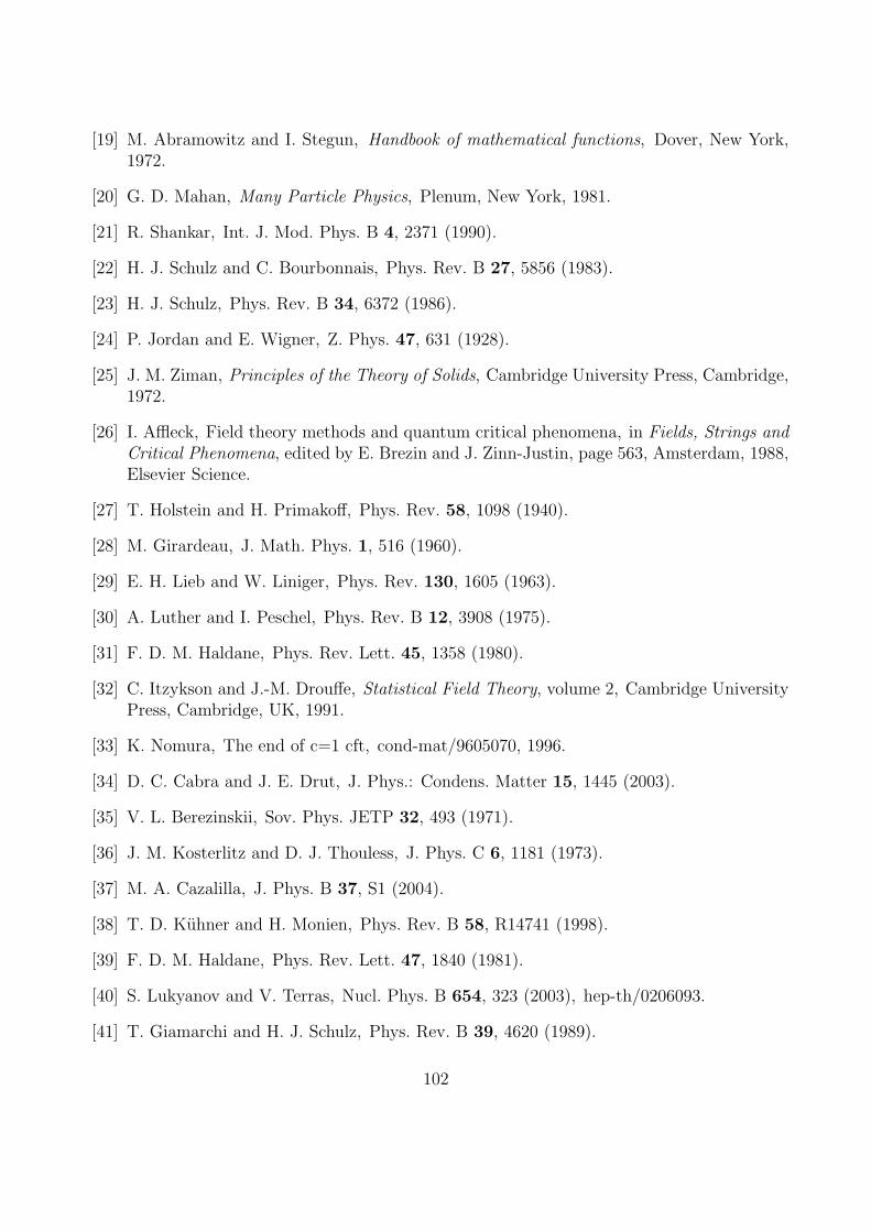
[19] M. Abramowitz and I. Stegun, Handbook of mathematical functions, Dover, New York,1972.
[20] G. D. Mahan, Many Particle Physics, Plenum, New York, 1981.
[21] R. Shankar, Int. J. Mod. Phys. B 4, 2371 (1990).
[22] H. J. Schulz and C. Bourbonnais, Phys. Rev. B 27, 5856 (1983).
[23] H. J. Schulz, Phys. Rev. B 34, 6372 (1986).
[24] P. Jordan and E. Wigner, Z. Phys. 47, 631 (1928).
[25] J. M. Ziman, Principles of the Theory of Solids, Cambridge University Press, Cambridge,1972.
[26] I. Affleck, Field theory methods and quantum critical phenomena, in Fields, Strings and
Critical Phenomena, edited by E. Brezin and J. Zinn-Justin, page 563, Amsterdam, 1988,Elsevier Science.
[27] T. Holstein and H. Primakoff, Phys. Rev. 58, 1098 (1940).
[28] M. Girardeau, J. Math. Phys. 1, 516 (1960).
[29] E. H. Lieb and W. Liniger, Phys. Rev. 130, 1605 (1963).
[30] A. Luther and I. Peschel, Phys. Rev. B 12, 3908 (1975).
[31] F. D. M. Haldane, Phys. Rev. Lett. 45, 1358 (1980).
[32] C. Itzykson and J.-M. Drouffe, Statistical Field Theory, volume 2, Cambridge UniversityPress, Cambridge, UK, 1991.
[33] K. Nomura, The end of c=1 cft, cond-mat/9605070, 1996.
[34] D. C. Cabra and J. E. Drut, J. Phys.: Condens. Matter 15, 1445 (2003).
[35] V. L. Berezinskii, Sov. Phys. JETP 32, 493 (1971).
[36] J. M. Kosterlitz and D. J. Thouless, J. Phys. C 6, 1181 (1973).
[37] M. A. Cazalilla, J. Phys. B 37, S1 (2004).
[38] T. D. Kuhner and H. Monien, Phys. Rev. B 58, R14741 (1998).
[39] F. D. M. Haldane, Phys. Rev. Lett. 47, 1840 (1981).
[40] S. Lukyanov and V. Terras, Nucl. Phys. B 654, 323 (2003), hep-th/0206093.
[41] T. Giamarchi and H. J. Schulz, Phys. Rev. B 39, 4620 (1989).
102
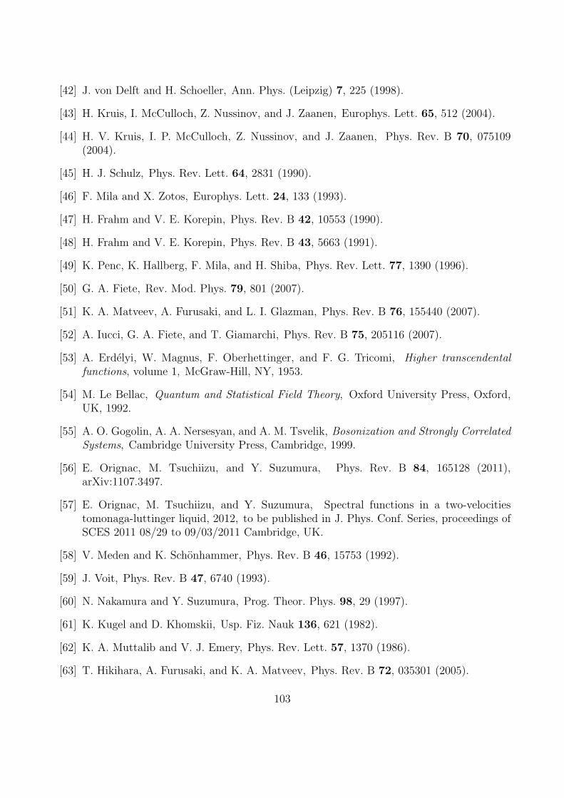
[42] J. von Delft and H. Schoeller, Ann. Phys. (Leipzig) 7, 225 (1998).
[43] H. Kruis, I. McCulloch, Z. Nussinov, and J. Zaanen, Europhys. Lett. 65, 512 (2004).
[44] H. V. Kruis, I. P. McCulloch, Z. Nussinov, and J. Zaanen, Phys. Rev. B 70, 075109(2004).
[45] H. J. Schulz, Phys. Rev. Lett. 64, 2831 (1990).
[46] F. Mila and X. Zotos, Europhys. Lett. 24, 133 (1993).
[47] H. Frahm and V. E. Korepin, Phys. Rev. B 42, 10553 (1990).
[48] H. Frahm and V. E. Korepin, Phys. Rev. B 43, 5663 (1991).
[49] K. Penc, K. Hallberg, F. Mila, and H. Shiba, Phys. Rev. Lett. 77, 1390 (1996).
[50] G. A. Fiete, Rev. Mod. Phys. 79, 801 (2007).
[51] K. A. Matveev, A. Furusaki, and L. I. Glazman, Phys. Rev. B 76, 155440 (2007).
[52] A. Iucci, G. A. Fiete, and T. Giamarchi, Phys. Rev. B 75, 205116 (2007).
[53] A. Erdelyi, W. Magnus, F. Oberhettinger, and F. G. Tricomi, Higher transcendental
functions, volume 1, McGraw-Hill, NY, 1953.
[54] M. Le Bellac, Quantum and Statistical Field Theory, Oxford University Press, Oxford,UK, 1992.
[55] A. O. Gogolin, A. A. Nersesyan, and A. M. Tsvelik, Bosonization and Strongly Correlated
Systems, Cambridge University Press, Cambridge, 1999.
[56] E. Orignac, M. Tsuchiizu, and Y. Suzumura, Phys. Rev. B 84, 165128 (2011),arXiv:1107.3497.
[57] E. Orignac, M. Tsuchiizu, and Y. Suzumura, Spectral functions in a two-velocitiestomonaga-luttinger liquid, 2012, to be published in J. Phys. Conf. Series, proceedings ofSCES 2011 08/29 to 09/03/2011 Cambridge, UK.
[58] V. Meden and K. Schonhammer, Phys. Rev. B 46, 15753 (1992).
[59] J. Voit, Phys. Rev. B 47, 6740 (1993).
[60] N. Nakamura and Y. Suzumura, Prog. Theor. Phys. 98, 29 (1997).
[61] K. Kugel and D. Khomskii, Usp. Fiz. Nauk 136, 621 (1982).
[62] K. A. Muttalib and V. J. Emery, Phys. Rev. Lett. 57, 1370 (1986).
[63] T. Hikihara, A. Furusaki, and K. A. Matveev, Phys. Rev. B 72, 035301 (2005).
103
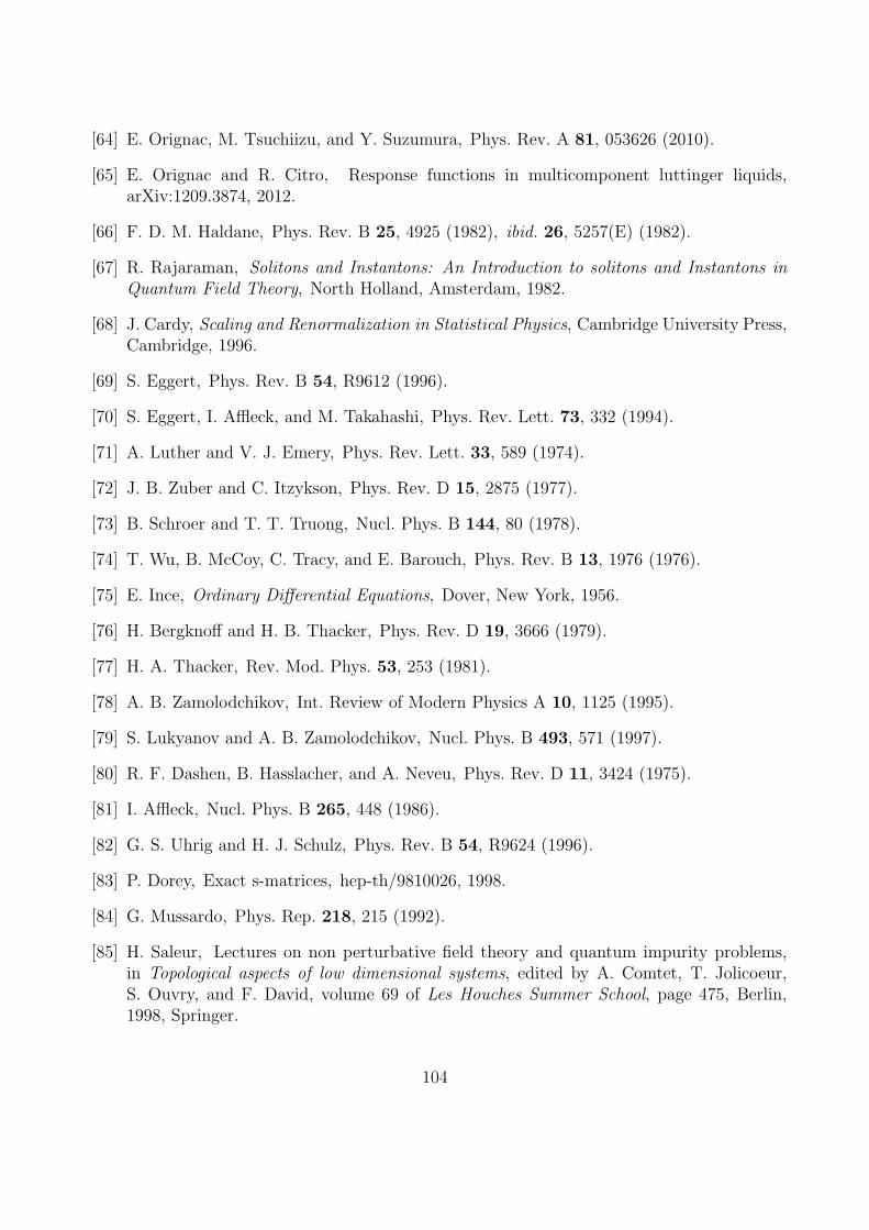
[64] E. Orignac, M. Tsuchiizu, and Y. Suzumura, Phys. Rev. A 81, 053626 (2010).
[65] E. Orignac and R. Citro, Response functions in multicomponent luttinger liquids,arXiv:1209.3874, 2012.
[66] F. D. M. Haldane, Phys. Rev. B 25, 4925 (1982), ibid. 26, 5257(E) (1982).
[67] R. Rajaraman, Solitons and Instantons: An Introduction to solitons and Instantons in
Quantum Field Theory, North Holland, Amsterdam, 1982.
[68] J. Cardy, Scaling and Renormalization in Statistical Physics, Cambridge University Press,Cambridge, 1996.
[69] S. Eggert, Phys. Rev. B 54, R9612 (1996).
[70] S. Eggert, I. Affleck, and M. Takahashi, Phys. Rev. Lett. 73, 332 (1994).
[71] A. Luther and V. J. Emery, Phys. Rev. Lett. 33, 589 (1974).
[72] J. B. Zuber and C. Itzykson, Phys. Rev. D 15, 2875 (1977).
[73] B. Schroer and T. T. Truong, Nucl. Phys. B 144, 80 (1978).
[74] T. Wu, B. McCoy, C. Tracy, and E. Barouch, Phys. Rev. B 13, 1976 (1976).
[75] E. Ince, Ordinary Differential Equations, Dover, New York, 1956.
[76] H. Bergknoff and H. B. Thacker, Phys. Rev. D 19, 3666 (1979).
[77] H. A. Thacker, Rev. Mod. Phys. 53, 253 (1981).
[78] A. B. Zamolodchikov, Int. Review of Modern Physics A 10, 1125 (1995).
[79] S. Lukyanov and A. B. Zamolodchikov, Nucl. Phys. B 493, 571 (1997).
[80] R. F. Dashen, B. Hasslacher, and A. Neveu, Phys. Rev. D 11, 3424 (1975).
[81] I. Affleck, Nucl. Phys. B 265, 448 (1986).
[82] G. S. Uhrig and H. J. Schulz, Phys. Rev. B 54, R9624 (1996).
[83] P. Dorey, Exact s-matrices, hep-th/9810026, 1998.
[84] G. Mussardo, Phys. Rep. 218, 215 (1992).
[85] H. Saleur, Lectures on non perturbative field theory and quantum impurity problems,in Topological aspects of low dimensional systems, edited by A. Comtet, T. Jolicoeur,S. Ouvry, and F. David, volume 69 of Les Houches Summer School, page 475, Berlin,1998, Springer.
104
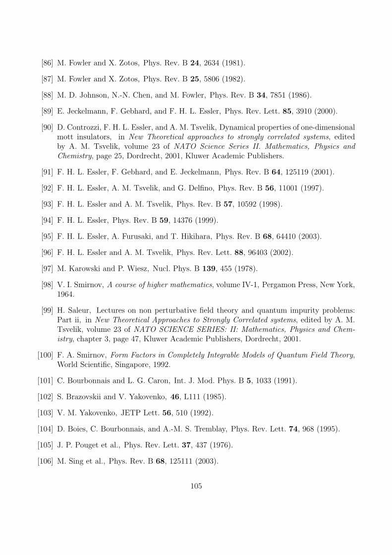
[86] M. Fowler and X. Zotos, Phys. Rev. B 24, 2634 (1981).
[87] M. Fowler and X. Zotos, Phys. Rev. B 25, 5806 (1982).
[88] M. D. Johnson, N.-N. Chen, and M. Fowler, Phys. Rev. B 34, 7851 (1986).
[89] E. Jeckelmann, F. Gebhard, and F. H. L. Essler, Phys. Rev. Lett. 85, 3910 (2000).
[90] D. Controzzi, F. H. L. Essler, and A. M. Tsvelik, Dynamical properties of one-dimensionalmott insulators, in New Theoretical approaches to strongly correlated systems, editedby A. M. Tsvelik, volume 23 of NATO Science Series II. Mathematics, Physics and
Chemistry, page 25, Dordrecht, 2001, Kluwer Academic Publishers.
[91] F. H. L. Essler, F. Gebhard, and E. Jeckelmann, Phys. Rev. B 64, 125119 (2001).
[92] F. H. L. Essler, A. M. Tsvelik, and G. Delfino, Phys. Rev. B 56, 11001 (1997).
[93] F. H. L. Essler and A. M. Tsvelik, Phys. Rev. B 57, 10592 (1998).
[94] F. H. L. Essler, Phys. Rev. B 59, 14376 (1999).
[95] F. H. L. Essler, A. Furusaki, and T. Hikihara, Phys. Rev. B 68, 64410 (2003).
[96] F. H. L. Essler and A. M. Tsvelik, Phys. Rev. Lett. 88, 96403 (2002).
[97] M. Karowski and P. Wiesz, Nucl. Phys. B 139, 455 (1978).
[98] V. I. Smirnov, A course of higher mathematics, volume IV-1, Pergamon Press, New York,1964.
[99] H. Saleur, Lectures on non perturbative field theory and quantum impurity problems:Part ii, in New Theoretical Approaches to Strongly Correlated systems, edited by A. M.Tsvelik, volume 23 of NATO SCIENCE SERIES: II: Mathematics, Physics and Chem-
istry, chapter 3, page 47, Kluwer Academic Publishers, Dordrecht, 2001.
[100] F. A. Smirnov, Form Factors in Completely Integrable Models of Quantum Field Theory,World Scientific, Singapore, 1992.
[101] C. Bourbonnais and L. G. Caron, Int. J. Mod. Phys. B 5, 1033 (1991).
[102] S. Brazovskii and V. Yakovenko, 46, L111 (1985).
[103] V. M. Yakovenko, JETP Lett. 56, 510 (1992).
[104] D. Boies, C. Bourbonnais, and A.-M. S. Tremblay, Phys. Rev. Lett. 74, 968 (1995).
[105] J. P. Pouget et al., Phys. Rev. Lett. 37, 437 (1976).
[106] M. Sing et al., Phys. Rev. B 68, 125111 (2003).
105
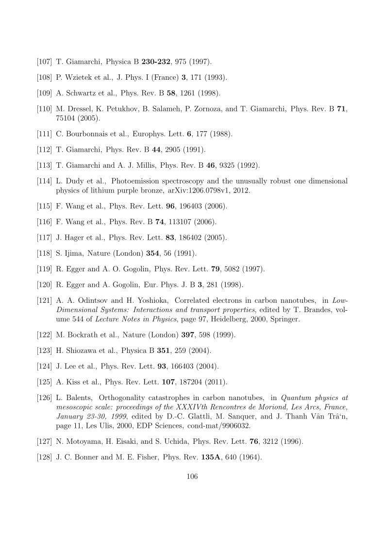
[107] T. Giamarchi, Physica B 230-232, 975 (1997).
[108] P. Wzietek et al., J. Phys. I (France) 3, 171 (1993).
[109] A. Schwartz et al., Phys. Rev. B 58, 1261 (1998).
[110] M. Dressel, K. Petukhov, B. Salameh, P. Zornoza, and T. Giamarchi, Phys. Rev. B 71,75104 (2005).
[111] C. Bourbonnais et al., Europhys. Lett. 6, 177 (1988).
[112] T. Giamarchi, Phys. Rev. B 44, 2905 (1991).
[113] T. Giamarchi and A. J. Millis, Phys. Rev. B 46, 9325 (1992).
[114] L. Dudy et al., Photoemission spectroscopy and the unusually robust one dimensionalphysics of lithium purple bronze, arXiv:1206.0798v1, 2012.
[115] F. Wang et al., Phys. Rev. Lett. 96, 196403 (2006).
[116] F. Wang et al., Phys. Rev. B 74, 113107 (2006).
[117] J. Hager et al., Phys. Rev. Lett. 83, 186402 (2005).
[118] S. Ijima, Nature (London) 354, 56 (1991).
[119] R. Egger and A. O. Gogolin, Phys. Rev. Lett. 79, 5082 (1997).
[120] R. Egger and A. Gogolin, Eur. Phys. J. B 3, 281 (1998).
[121] A. A. Odintsov and H. Yoshioka, Correlated electrons in carbon nanotubes, in Low-
Dimensional Systems: Interactions and transport properties, edited by T. Brandes, vol-ume 544 of Lecture Notes in Physics, page 97, Heidelberg, 2000, Springer.
[122] M. Bockrath et al., Nature (London) 397, 598 (1999).
[123] H. Shiozawa et al., Physica B 351, 259 (2004).
[124] J. Lee et al., Phys. Rev. Lett. 93, 166403 (2004).
[125] A. Kiss et al., Phys. Rev. Lett. 107, 187204 (2011).
[126] L. Balents, Orthogonality catastrophes in carbon nanotubes, in Quantum physics at
mesoscopic scale: proceedings of the XXXIVth Rencontres de Moriond, Les Arcs, France,
January 23-30, 1999, edited by D.-C. Glattli, M. Sanquer, and J. Thanh Van Tra‘n,page 11, Les Ulis, 2000, EDP Sciences, cond-mat/9906032.
[127] N. Motoyama, H. Eisaki, and S. Uchida, Phys. Rev. Lett. 76, 3212 (1996).
[128] J. C. Bonner and M. E. Fisher, Phys. Rev. 135A, 640 (1964).
106
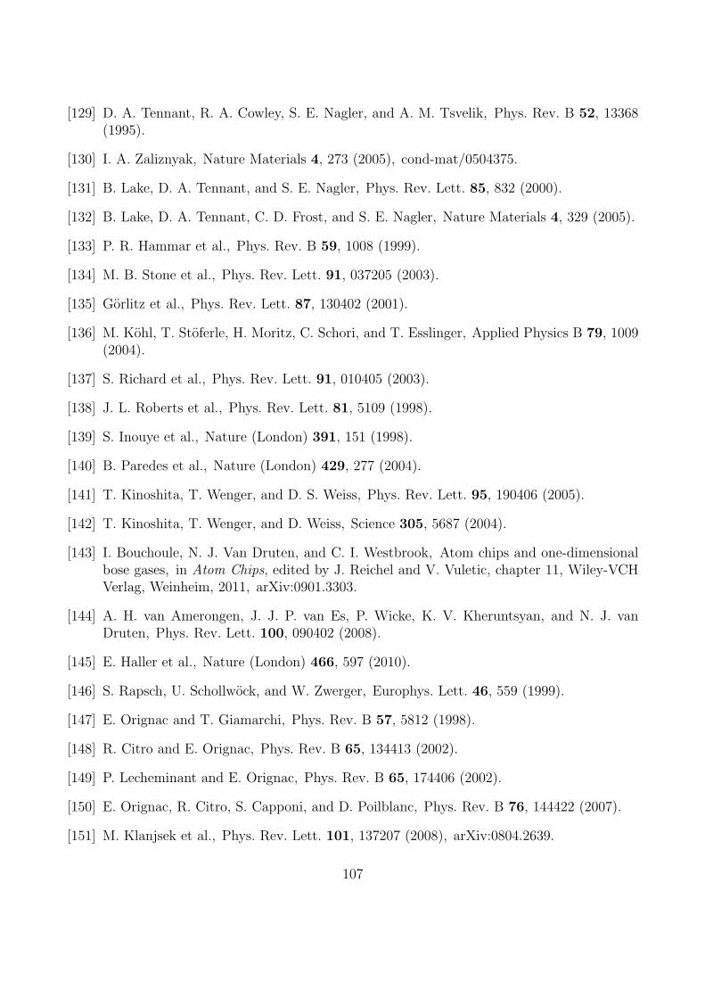
[129] D. A. Tennant, R. A. Cowley, S. E. Nagler, and A. M. Tsvelik, Phys. Rev. B 52, 13368(1995).
[130] I. A. Zaliznyak, Nature Materials 4, 273 (2005), cond-mat/0504375.
[131] B. Lake, D. A. Tennant, and S. E. Nagler, Phys. Rev. Lett. 85, 832 (2000).
[132] B. Lake, D. A. Tennant, C. D. Frost, and S. E. Nagler, Nature Materials 4, 329 (2005).
[133] P. R. Hammar et al., Phys. Rev. B 59, 1008 (1999).
[134] M. B. Stone et al., Phys. Rev. Lett. 91, 037205 (2003).
[135] Gorlitz et al., Phys. Rev. Lett. 87, 130402 (2001).
[136] M. Kohl, T. Stoferle, H. Moritz, C. Schori, and T. Esslinger, Applied Physics B 79, 1009(2004).
[137] S. Richard et al., Phys. Rev. Lett. 91, 010405 (2003).
[138] J. L. Roberts et al., Phys. Rev. Lett. 81, 5109 (1998).
[139] S. Inouye et al., Nature (London) 391, 151 (1998).
[140] B. Paredes et al., Nature (London) 429, 277 (2004).
[141] T. Kinoshita, T. Wenger, and D. S. Weiss, Phys. Rev. Lett. 95, 190406 (2005).
[142] T. Kinoshita, T. Wenger, and D. Weiss, Science 305, 5687 (2004).
[143] I. Bouchoule, N. J. Van Druten, and C. I. Westbrook, Atom chips and one-dimensionalbose gases, in Atom Chips, edited by J. Reichel and V. Vuletic, chapter 11, Wiley-VCHVerlag, Weinheim, 2011, arXiv:0901.3303.
[144] A. H. van Amerongen, J. J. P. van Es, P. Wicke, K. V. Kheruntsyan, and N. J. vanDruten, Phys. Rev. Lett. 100, 090402 (2008).
[145] E. Haller et al., Nature (London) 466, 597 (2010).
[146] S. Rapsch, U. Schollwock, and W. Zwerger, Europhys. Lett. 46, 559 (1999).
[147] E. Orignac and T. Giamarchi, Phys. Rev. B 57, 5812 (1998).
[148] R. Citro and E. Orignac, Phys. Rev. B 65, 134413 (2002).
[149] P. Lecheminant and E. Orignac, Phys. Rev. B 65, 174406 (2002).
[150] E. Orignac, R. Citro, S. Capponi, and D. Poilblanc, Phys. Rev. B 76, 144422 (2007).
[151] M. Klanjsek et al., Phys. Rev. Lett. 101, 137207 (2008), arXiv:0804.2639.
107
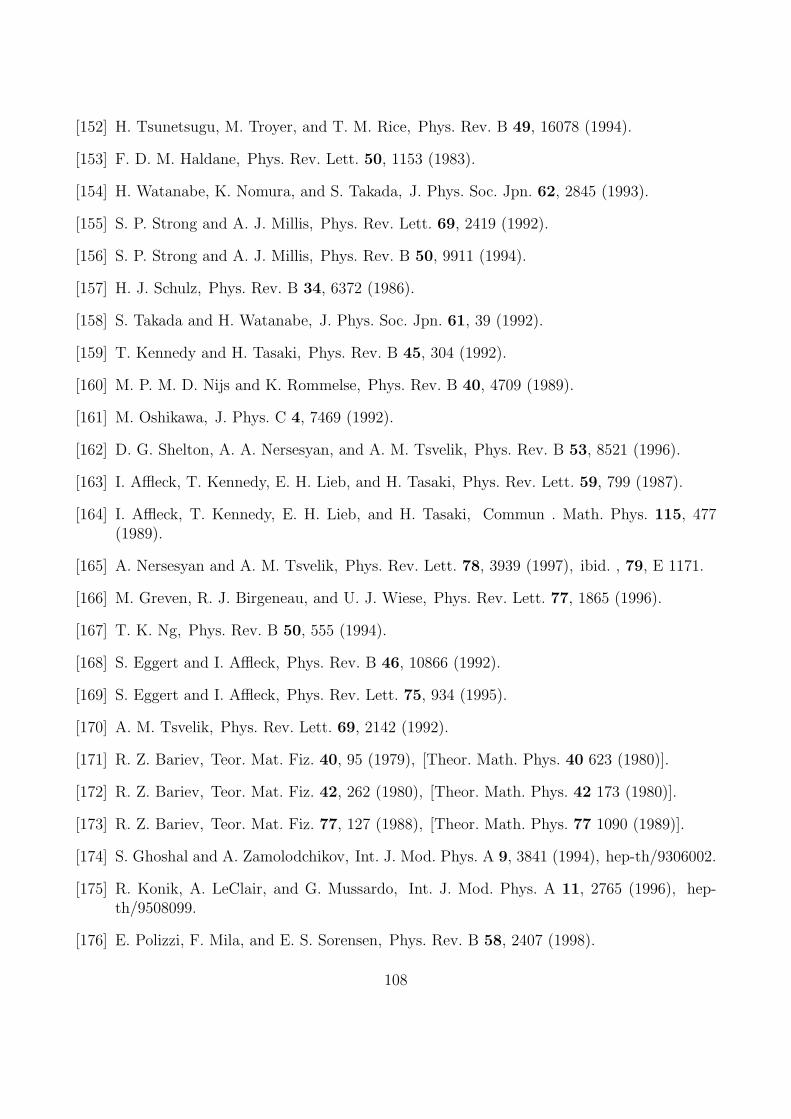
[152] H. Tsunetsugu, M. Troyer, and T. M. Rice, Phys. Rev. B 49, 16078 (1994).
[153] F. D. M. Haldane, Phys. Rev. Lett. 50, 1153 (1983).
[154] H. Watanabe, K. Nomura, and S. Takada, J. Phys. Soc. Jpn. 62, 2845 (1993).
[155] S. P. Strong and A. J. Millis, Phys. Rev. Lett. 69, 2419 (1992).
[156] S. P. Strong and A. J. Millis, Phys. Rev. B 50, 9911 (1994).
[157] H. J. Schulz, Phys. Rev. B 34, 6372 (1986).
[158] S. Takada and H. Watanabe, J. Phys. Soc. Jpn. 61, 39 (1992).
[159] T. Kennedy and H. Tasaki, Phys. Rev. B 45, 304 (1992).
[160] M. P. M. D. Nijs and K. Rommelse, Phys. Rev. B 40, 4709 (1989).
[161] M. Oshikawa, J. Phys. C 4, 7469 (1992).
[162] D. G. Shelton, A. A. Nersesyan, and A. M. Tsvelik, Phys. Rev. B 53, 8521 (1996).
[163] I. Affleck, T. Kennedy, E. H. Lieb, and H. Tasaki, Phys. Rev. Lett. 59, 799 (1987).
[164] I. Affleck, T. Kennedy, E. H. Lieb, and H. Tasaki, Commun . Math. Phys. 115, 477(1989).
[165] A. Nersesyan and A. M. Tsvelik, Phys. Rev. Lett. 78, 3939 (1997), ibid. , 79, E 1171.
[166] M. Greven, R. J. Birgeneau, and U. J. Wiese, Phys. Rev. Lett. 77, 1865 (1996).
[167] T. K. Ng, Phys. Rev. B 50, 555 (1994).
[168] S. Eggert and I. Affleck, Phys. Rev. B 46, 10866 (1992).
[169] S. Eggert and I. Affleck, Phys. Rev. Lett. 75, 934 (1995).
[170] A. M. Tsvelik, Phys. Rev. Lett. 69, 2142 (1992).
[171] R. Z. Bariev, Teor. Mat. Fiz. 40, 95 (1979), [Theor. Math. Phys. 40 623 (1980)].
[172] R. Z. Bariev, Teor. Mat. Fiz. 42, 262 (1980), [Theor. Math. Phys. 42 173 (1980)].
[173] R. Z. Bariev, Teor. Mat. Fiz. 77, 127 (1988), [Theor. Math. Phys. 77 1090 (1989)].
[174] S. Ghoshal and A. Zamolodchikov, Int. J. Mod. Phys. A 9, 3841 (1994), hep-th/9306002.
[175] R. Konik, A. LeClair, and G. Mussardo, Int. J. Mod. Phys. A 11, 2765 (1996), hep-th/9508099.
[176] E. Polizzi, F. Mila, and E. S. Sorensen, Phys. Rev. B 58, 2407 (1998).
108
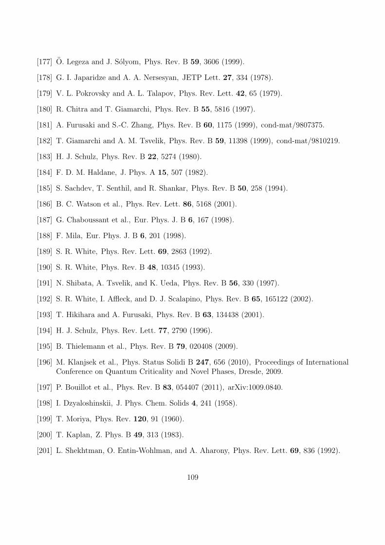
[177] O. Legeza and J. Solyom, Phys. Rev. B 59, 3606 (1999).
[178] G. I. Japaridze and A. A. Nersesyan, JETP Lett. 27, 334 (1978).
[179] V. L. Pokrovsky and A. L. Talapov, Phys. Rev. Lett. 42, 65 (1979).
[180] R. Chitra and T. Giamarchi, Phys. Rev. B 55, 5816 (1997).
[181] A. Furusaki and S.-C. Zhang, Phys. Rev. B 60, 1175 (1999), cond-mat/9807375.
[182] T. Giamarchi and A. M. Tsvelik, Phys. Rev. B 59, 11398 (1999), cond-mat/9810219.
[183] H. J. Schulz, Phys. Rev. B 22, 5274 (1980).
[184] F. D. M. Haldane, J. Phys. A 15, 507 (1982).
[185] S. Sachdev, T. Senthil, and R. Shankar, Phys. Rev. B 50, 258 (1994).
[186] B. C. Watson et al., Phys. Rev. Lett. 86, 5168 (2001).
[187] G. Chaboussant et al., Eur. Phys. J. B 6, 167 (1998).
[188] F. Mila, Eur. Phys. J. B 6, 201 (1998).
[189] S. R. White, Phys. Rev. Lett. 69, 2863 (1992).
[190] S. R. White, Phys. Rev. B 48, 10345 (1993).
[191] N. Shibata, A. Tsvelik, and K. Ueda, Phys. Rev. B 56, 330 (1997).
[192] S. R. White, I. Affleck, and D. J. Scalapino, Phys. Rev. B 65, 165122 (2002).
[193] T. Hikihara and A. Furusaki, Phys. Rev. B 63, 134438 (2001).
[194] H. J. Schulz, Phys. Rev. Lett. 77, 2790 (1996).
[195] B. Thielemann et al., Phys. Rev. B 79, 020408 (2009).
[196] M. Klanjsek et al., Phys. Status Solidi B 247, 656 (2010), Proceedings of InternationalConference on Quantum Criticality and Novel Phases, Dresde, 2009.
[197] P. Bouillot et al., Phys. Rev. B 83, 054407 (2011), arXiv:1009.0840.
[198] I. Dzyaloshinskii, J. Phys. Chem. Solids 4, 241 (1958).
[199] T. Moriya, Phys. Rev. 120, 91 (1960).
[200] T. Kaplan, Z. Phys. B 49, 313 (1983).
[201] L. Shekhtman, O. Entin-Wohlman, and A. Aharony, Phys. Rev. Lett. 69, 836 (1992).
109
[202] L. Shekhtman, A. Aharony, and O. Entin-Wohlman, Phys. Rev. B 47, 174 (1993).
[203] D. Dender, P. R. Hammar, D. H. Reich, C. Broholm, and G. Aeppli, Phys. Rev. Lett.79, 1750 (1997).
[204] M. Oshikawa and I. Affleck, Phys. Rev. Lett. 79, 2883 (1997).
[205] I. Affleck and M. Oshikawa, Phys. Rev. B 60, 1039 (1999), Phys. Rev. B 62, 9200(E)(2000).
[206] D. N. Aristov and S. V. Maleyev, Phys. Rev. B 62, R751 (2000).
[207] S. A. Zvyagin, A. K. Kolezhuk, J. Krzystek, and R. Feyerherm, Phys. Rev. Lett. 93,027201 (2004).
[208] S. A. Zvyagin, A. K. Kolezhuk, J. Krzystek, and R. Feyerherm, Phys. Rev. Lett. 95,017207 (2005).
[209] S. A. Zvyagin et al., Phys. Rev. B 83, 060409 (2011).
[210] M. Kohgi et al., Phys. Rev. Lett. 86, 2439 (2001).
[211] R. Matysiak, G. Kamieniarz, P. Gegenwart, and A. Ochiai, Phys. Rev. B 79, 224413(2009).
[212] M. Kenzelmann, Y. Chen, C. Broholm, D. H. Reich, and Y. Qiu, Phys. Rev. Lett. 93,017204 (2004).
[213] S. Bertaina, V. A. Pashchenko, A. Stepanov, T. Masuda, and K. Uchinokura, Phys. Rev.Lett. 92, 057203 (2004).
[214] M. Herak et al., Phys. Rev. B 84, 184436 (2011).
[215] I. Umegaki, H. Tanaka, T. Ono, H. Uekusa, and H. Nojiri, Phys. Rev. B 79, 184401(2009).
[216] I. Umegaki, H. Tanaka, T. Ono, M. Oshikawa, and K. Sakai, Phys. Rev. B 85, 144423(2012).
[217] A. M. Tsvelik, Phys. Rev. B 42, 10499 (1990).
[218] M. Clemancey et al., Phys. Rev. Lett. 97, 167204 (2006).
[219] S. Miyahara et al., Phys. Rev. B 75, 184402 (2006).
[220] S. Capponi and D. Poilblanc, Phys. Rev. B 75, 092406 (2007), cond-mat/0612162.
[221] G. Chaboussant et al., Eur. Phys. J. B 6, 167 (1998).
[222] P. A. Fleury and R. Loudon, Phys. Rev. 166, 514 (1968).
110
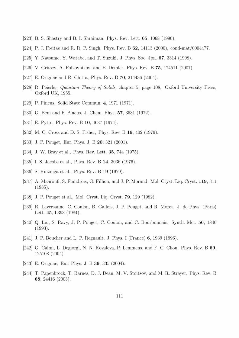
[223] B. S. Shastry and B. I. Shraiman, Phys. Rev. Lett. 65, 1068 (1990).
[224] P. J. Freitas and R. R. P. Singh, Phys. Rev. B 62, 14113 (2000), cond-mat/0004477.
[225] Y. Natsume, Y. Watabe, and T. Suzuki, J. Phys. Soc. Jpn. 67, 3314 (1998).
[226] V. Gritsev, A. Polkovnikov, and E. Demler, Phys. Rev. B 75, 174511 (2007).
[227] E. Orignac and R. Chitra, Phys. Rev. B 70, 214436 (2004).
[228] R. Peierls, Quantum Theory of Solids, chapter 5, page 108, Oxford University Press,Oxford UK, 1955.
[229] P. Pincus, Solid State Commun. 4, 1971 (1971).
[230] G. Beni and P. Pincus, J. Chem. Phys. 57, 3531 (1972).
[231] E. Pytte, Phys. Rev. B 10, 4637 (1974).
[232] M. C. Cross and D. S. Fisher, Phys. Rev. B 19, 402 (1979).
[233] J. P. Pouget, Eur. Phys. J. B 20, 321 (2001).
[234] J. W. Bray et al., Phys. Rev. Lett. 35, 744 (1975).
[235] I. S. Jacobs et al., Phys. Rev. B 14, 3036 (1976).
[236] S. Huizinga et al., Phys. Rev. B 19 (1979).
[237] A. Maaroufi, S. Flandrois, G. Fillion, and J. P. Morand, Mol. Cryst. Liq. Cryst. 119, 311(1985).
[238] J. P. Pouget et al., Mol. Cryst. Liq. Cryst. 79, 129 (1982).
[239] R. Laversanne, C. Coulon, B. Gallois, J. P. Pouget, and R. Moret, J. de Phys. (Paris)Lett. 45, L393 (1984).
[240] Q. Liu, S. Ravy, J. P. Pouget, C. Coulon, and C. Bourbonnais, Synth. Met. 56, 1840(1993).
[241] J. P. Boucher and L. P. Regnault, J. Phys. I (France) 6, 1939 (1996).
[242] G. Caimi, L. Degiorgi, N. N. Kovaleva, P. Lemmens, and F. C. Chou, Phys. Rev. B 69,125108 (2004).
[243] E. Orignac, Eur. Phys. J. B 39, 335 (2004).
[244] T. Papenbrock, T. Barnes, D. J. Dean, M. V. Stoitsov, and M. R. Strayer, Phys. Rev. B68, 24416 (2003).
111
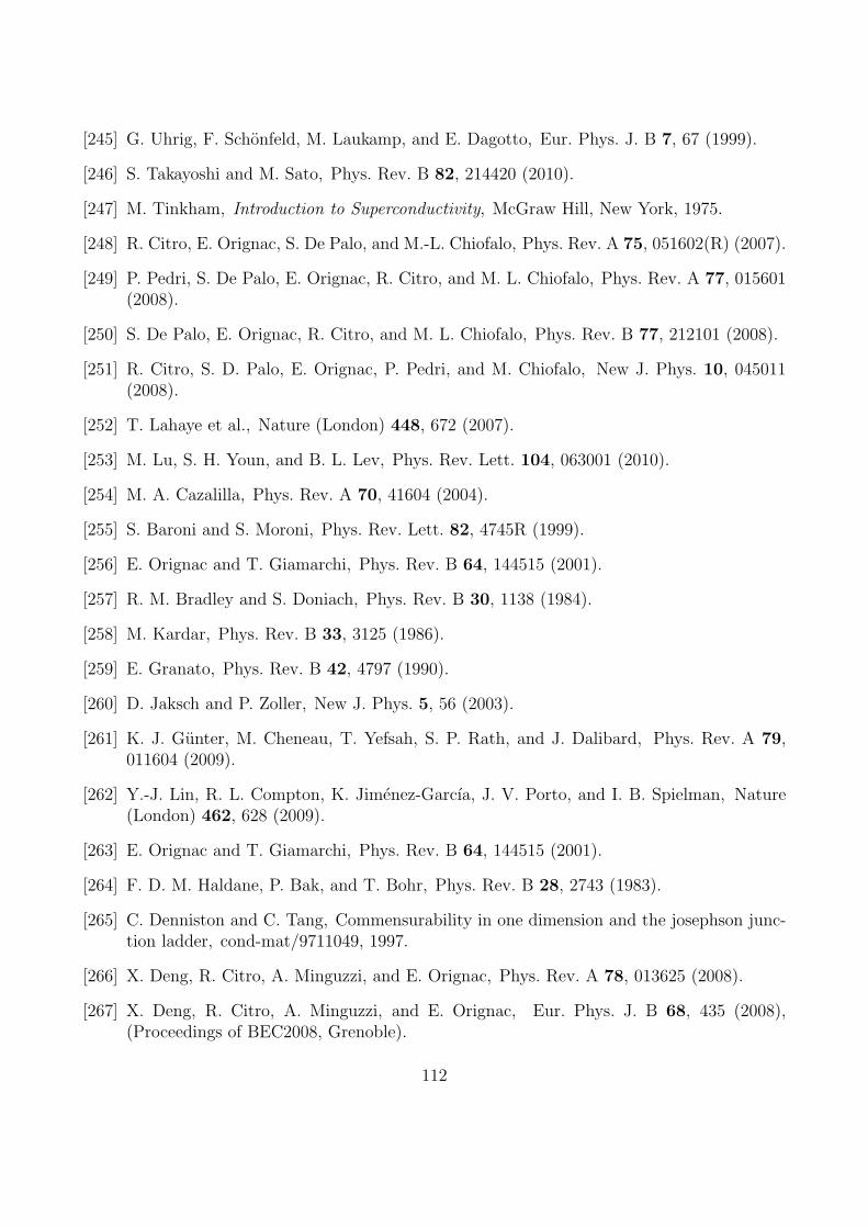
[245] G. Uhrig, F. Schonfeld, M. Laukamp, and E. Dagotto, Eur. Phys. J. B 7, 67 (1999).
[246] S. Takayoshi and M. Sato, Phys. Rev. B 82, 214420 (2010).
[247] M. Tinkham, Introduction to Superconductivity, McGraw Hill, New York, 1975.
[248] R. Citro, E. Orignac, S. De Palo, and M.-L. Chiofalo, Phys. Rev. A 75, 051602(R) (2007).
[249] P. Pedri, S. De Palo, E. Orignac, R. Citro, and M. L. Chiofalo, Phys. Rev. A 77, 015601(2008).
[250] S. De Palo, E. Orignac, R. Citro, and M. L. Chiofalo, Phys. Rev. B 77, 212101 (2008).
[251] R. Citro, S. D. Palo, E. Orignac, P. Pedri, and M. Chiofalo, New J. Phys. 10, 045011(2008).
[252] T. Lahaye et al., Nature (London) 448, 672 (2007).
[253] M. Lu, S. H. Youn, and B. L. Lev, Phys. Rev. Lett. 104, 063001 (2010).
[254] M. A. Cazalilla, Phys. Rev. A 70, 41604 (2004).
[255] S. Baroni and S. Moroni, Phys. Rev. Lett. 82, 4745R (1999).
[256] E. Orignac and T. Giamarchi, Phys. Rev. B 64, 144515 (2001).
[257] R. M. Bradley and S. Doniach, Phys. Rev. B 30, 1138 (1984).
[258] M. Kardar, Phys. Rev. B 33, 3125 (1986).
[259] E. Granato, Phys. Rev. B 42, 4797 (1990).
[260] D. Jaksch and P. Zoller, New J. Phys. 5, 56 (2003).
[261] K. J. Gunter, M. Cheneau, T. Yefsah, S. P. Rath, and J. Dalibard, Phys. Rev. A 79,011604 (2009).
[262] Y.-J. Lin, R. L. Compton, K. Jimenez-Garcıa, J. V. Porto, and I. B. Spielman, Nature(London) 462, 628 (2009).
[263] E. Orignac and T. Giamarchi, Phys. Rev. B 64, 144515 (2001).
[264] F. D. M. Haldane, P. Bak, and T. Bohr, Phys. Rev. B 28, 2743 (1983).
[265] C. Denniston and C. Tang, Commensurability in one dimension and the josephson junc-tion ladder, cond-mat/9711049, 1997.
[266] X. Deng, R. Citro, A. Minguzzi, and E. Orignac, Phys. Rev. A 78, 013625 (2008).
[267] X. Deng, R. Citro, A. Minguzzi, and E. Orignac, Eur. Phys. J. B 68, 435 (2008),(Proceedings of BEC2008, Grenoble).
112
[268] S. Aubry and G. Andre, Ann. Isr. Phys. Soc. 3, 113 (1980).
[269] D. J. Thouless, Phys. Rep. 13, 93 (1974).
[270] I. M. Lifshitz, L. P. Pastur, and S. Gredeskul, Introduction to the theory of disordered
systems, Wiley and Sons, New York, 1988.
[271] G. Roati et al., Nature (London) 453, 895 (2008).
[272] G. Roux et al., Phys. Rev. A 78, 023628 (2008).
113