Quantum Mechanics

1 Big Picture

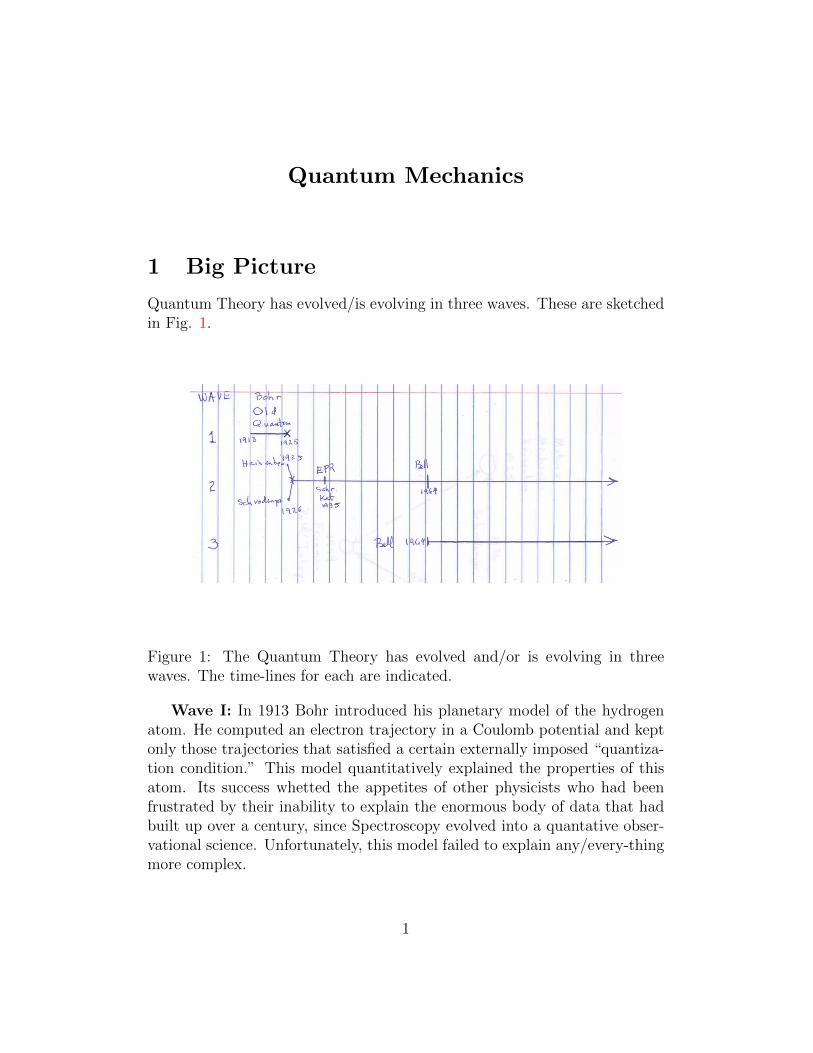
Quantum Theory has evolved/is evolving in three waves. These are sketchedin Fig. 1.

Figure 1: The Quantum Theory has evolved and/or is evolving in threewaves. The time-lines for each are indicated.

Wave I: In 1913 Bohr introduced his planetary model of the hydrogenatom. He computed an electron trajectory in a Coulomb potential and keptonly those trajectories that satisfied a certain externally imposed “quantiza-tion condition.” This model quantitatively explained the properties of thisatom. Its success whetted the appetites of other physicists who had beenfrustrated by their inability to explain the enormous body of data that hadbuilt up over a century, since Spectroscopy evolved into a quantative obser-vational science. Unfortunately, this model failed to explain any/every-thingmore complex.

1

Wave IIa - Matrix Mechanics: In 1925 Heisenberg (Bohr’s pro-tege) realized that tables of transition frequencies can be treated as ma-trices. He formulated a quantum theory in terms of matrices. In this the-ory these frequencies, or matrix elements, are the only observables. “If itisn’t observed, it doesn’t exist.” Born, Heisenberg, and Jordan complete the“DreiMannerArbeit” (“Three men’s work”) in which they create a formalprescription (algorithm) that allows them to start from a Hamiltonian thatdescribes a classical atomic puzzle (planetary model of an atom) and convertit to a Matrix Mechanics description of the same puzzle. This algorithm wasvery difficult to apply, especially given the fact that no physicists knew howto work with, or even knew about, matrices at that time. Only Pauli wasable to use this prescription to solve the hydrogen atom problem. His solu-tion involved not only the obvious symmetry (rotation symmetry, or SO(3)symmetry), but the even larger symmetry [SO(4), SO(3, 1)] presented bythe invariance of the Runge-Lenz vector. The “DreiMannerArbeit” servedas the template for Herbert Goldstein’s beautiful book Classical Mechanics,Addison-Wesley, 1950. This book was written with an eye to tailoring thefoundations of Classical Mechanics for Quantum Mechanics courses.

Wave IIb - Wave Mechanics: In 1926 Schrodinger submitted his firstWave Mechanics paper (QAEP-1). It was sent to the journal simultaneously(and independently of) Pauli’s solution of the hydrogen atom problem usingMatrix Mechanics. In his paper Schrodinger formulated the hydrogen atomproblem as a partial differential equation. At the time partial differentialequations were far more familiar to physicists than matrices. In this paper hesolved the hydrogen atom for both the discrete and the continuous spectrumusing the (then) widely known and powerful techniques of complex variabletheory.

Six months later Schrodinger showed the equivalence of his Wave Mechan-ics with the Matrix Mechanics of Born, Heisenberg, and Jordan. In the con-test between partial differential equations and matrices, PDEs (Schrodinger)trumped matrices (Heisenberg) hands down. To get back into the ring,Heisenberg proposed the Uncertainty Principle in 1927.

In later years (after 1943) effective ways of solving PDEs by convertingthem to matrix equations are supplementing/ have supplemented Wave Me-chanics. And later yet, in 1949 Feynman proposed a third very intuitive wayof formulating Quantum Theory as a sum-over-all-paths theory.

The relations among these three ways of formulating Quantum Mechanicsis summarized in Fig. 2.

2

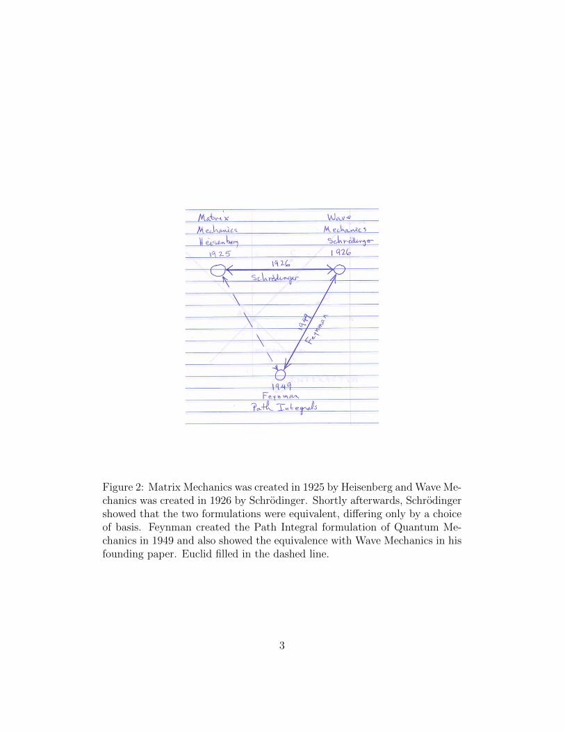
Figure 2: Matrix Mechanics was created in 1925 by Heisenberg and Wave Me-chanics was created in 1926 by Schrodinger. Shortly afterwards, Schrodingershowed that the two formulations were equivalent, differing only by a choiceof basis. Feynman created the Path Integral formulation of Quantum Me-chanics in 1949 and also showed the equivalence with Wave Mechanics in hisfounding paper. Euclid filled in the dashed line.

3

III - Schrodinger and Einstein Strike Back: In 1935 both Schrodingerand Einstein vented their frustration with Quantum Theory. The EPR man-ifesto proposed a gedankenexperiment to highlight the incompleteness ofquantum theory as then formulated. They introduced a concept that wenow call “entanglement” (Schrodinger’s term for it is ‘intrication’). Thispaper encouraged Schrodinger to express his disenchantment with his ownchild. He did so by proposing the “Cat Paradox”. This is now usually ad-dressed under the name “decoherence”, while the EPR challenge is discussedin terms of “Spooky Action at a Distance”.

The EPR challenge seemed to be a purely philosophical debate betweenEinstein and Bohr until

a. In 1957 Bohm proposed a different way to formulate the experiment.

b. In 1964 Bell showed how Einstein and Bohr predicted different outcomesfor a class of experiments.

The result (so far): Before, only determinism could create correlations amongmeasurements. Now, there is a brand new resource, measurement, that cancreate correlations. We (still) don’t fully understand how Nature works.

All these developments took place subject to the constraints of Thermo-dynamics and its Big Brother, Statistical Mechanics. The principles of thesesubjects, especially in the hands of Maxwell, Boltzmann, Wein, Planck, andEinstein, placed severe constraints on the evolution of the Quantum Theoryof Radiation. They continue to do so, at least as of 1976 with the discoveryof Black Hole Thermodynamics and Hawking Radiation.

2 Elaboration

Wave I: Bohr’s “Old Quantum Theory” is a beautiful theory for historicalstudy. We won’t study it. It is not correct. In 1917 Einstein pointedly showedthat it couldn’t be correct. In a paper that was largely ignored (uncited for50 years) he showed that the Bohr-Sommerfeld quantization condition ontrajectories could be written in the form∮

Ci

p · dq = nih (1)

4

where the contour integral is taken around each of k independent loops of a k-degree of freedom system. This works when the classical system is integrableand trajectories live on a k-dimensional torus in a 2k-dimensional phasespace. The loops Ci form a basis for the homotopy group of the torus T k.If the system is not integrable this quantization condition falls apart. Thisfatal objection to the Old Quantum Theory did not kill it: It lasted until itcould be replaced by (first) Matrix Mechanics and (very shortly afterward)by Wave Mechanics.

The Old Quantum Theory gave rise to several concepts that were radicaland fascinating at the time, but have grown old and useless, if not outrightwrong, at the present. Nevertheless, academic inertia is such that these (e.g,Correspondence Principle) have failed to be relegated to oblivion.

Wave II: Schrodinger did two things in the first two pages of his firstpaper on Wave Mecanics:

a. He introduced a variational formulation for a field ψ(x) (now called “wavefunction”):

J =∫ (

K(∇ψ(x))2 + V (x)(ψ(x))2)dV

δJ = 0 K =h2

2m

(2)

He also pointed out that the action J is a quadratic form in both ψ and∇ψ. The implications are profound (fast forward many years): Thisvariation equation can “easily” be solved using matrix methods.

b. He reduced the variational problem to a linear equation involving thepotential V (x) and the second derivative operator ∇2 using a stan-dard integration by parts procedure and separately addressing bound-ary conditions. Thus the Schrodinger equation is a consequence of thevariational formulation of Wave Mechanics:

−∇(K∇ψ) + V ψ = Eψ (3)

In this equation the energy, E, enters as a Lagrange multiplier and hasa physical interpretation as energy.

The remainder of his first paper on Wave Mechanics is devoted to solvingthe hydrogen atom problem and wrestling with the interpretation of the newfield, ψ, that he introduced.

5

3 Summary of Schrodinger’s Annus Mirabilis

of 1926

Schrodinger published six fundamental papers on Quantum Mechanics in1926. They are collected in: Collected Papers on Quantum Mechanics -Schrodinger, AMS Chelsea Publishing Co., Providence, RI, 2001, 2003. Thiscollection also contains three later papers and four of his lectures.

The six papers are summarized here.

Quantization as an Eigenvalue Problem I.a. Variational formulation, quadratic form in ψ and ∇ψb. Differential equation formc. Solution hydrogen atomd. ? What have I wrought ?

Quantization as an Eigenvalue Problem II.a. Wave optics — Wave mechanics analogyb. Harmonic oscillatorc. Rigid rotorsd. Rotating oscillator as model for moleculese. ? What have I wrought ?

The Continuous Transformation from Micro- to Macro-Mechanicsa. Quantum system closest to classical harmonic oscillatorb. Coherent states (now foundation of Quantum Optics)

On the Relation Between the Quantum Mechanics of Born, Heisenberg,and Jordan and that of Schrodinger

a. Two two are equivalentb. They differ by a change of basis

Quantization as an Eigenvalue Problem III.a. Time independent perturbation theory introducedb. Applied to describe the Stark effect

Quantization as an Eigenvalue Problem IV.a. Time dependent Schrodinger Equation introducedb. Time dependent perturbation theory introducedc. Excited atoms, discrete and continuous spectrad. Resonancese. Magnetic and relativistic generalizationsf. ? What have I wrought ?

6

4 Bell and the Third Wave

Bohr and Einstein carried out an argument about Quantum Mechanics thatwas unresolved at their deaths. In essence, Einstein argued that the ulti-mately measured properties of a physical system were written into the waveat the time of its creation. Bohr argued that they were created only at thetime of the measuremewnt of the wavefunction. The rest of the Physics com-munity regarded their argument as akin to the medieval argument about howmany angels could dance on the head of a pin.

With the greatest of apologies to Bohr and Einstein, their argument onthe foundations of Quantum Mechanics is summarized in Fig. 3. In thisfigure a measurement is carried out at spacetime point A. The question is:Are measurements at spacetime points B, C, D correlated with those at A?Everybody agrees that measurements at A and B can be correlated, since Bcan be connected to A by a time-like signal. Same for A and C. Everybodyalso agrees that measurements at B and C can also be correlated, even ifthese two points are space-like separated, if both are in the lightcone of A,as both can be influenced by events at A.

Einstein argues that events at A cannot influence measurements at Dwhen A and D are spacelike separated. Bohr argues that measurements atA and D can be correlated provided that the two have interacted sometimein the past and they are in an “entangled” state.

Experiments have been done. At present, they show that Bohr is correctand Einstein is not. This raises philosophical issues. These resutls showus that we do not “understand” the working of Nature. These results alsoopen a brand new resource for Physicists. This resource allows correlationsamong events in nature to be created in a third way: Not only by directcausality (B and A in Fig. 3) and indirect causality (B and C in Fig. 3),but also through “entanglement”. This resource is currently being exploitedin securing communications.

7

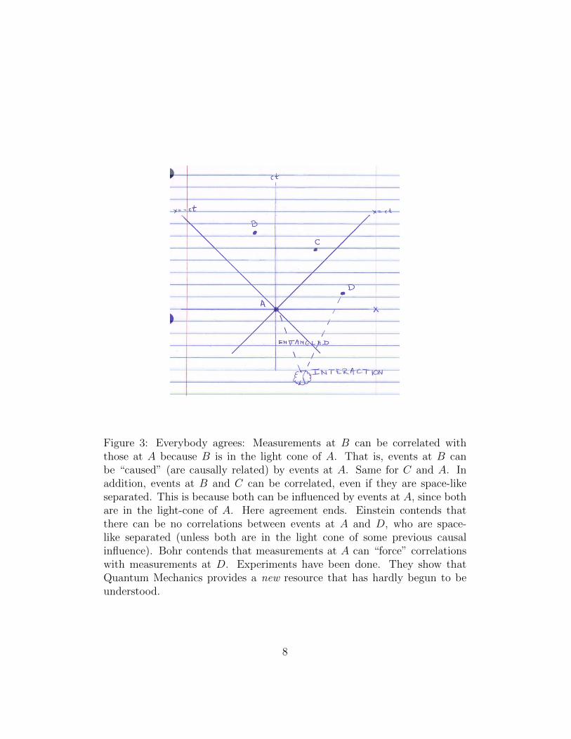
Figure 3: Everybody agrees: Measurements at B can be correlated withthose at A because B is in the light cone of A. That is, events at B canbe “caused” (are causally related) by events at A. Same for C and A. Inaddition, events at B and C can be correlated, even if they are space-likeseparated. This is because both can be influenced by events at A, since bothare in the light-cone of A. Here agreement ends. Einstein contends thatthere can be no correlations between events at A and D, who are space-like separated (unless both are in the light cone of some previous causalinfluence). Bohr contends that measurements at A can “force” correlationswith measurements at D. Experiments have been done. They show thatQuantum Mechanics provides a new resource that has hardly begun to beunderstood.

8

5 Schrodinger’s First Paper

Schrodinger’s initial formulation of Wave Mechanics was through the follow-ing variational principle:

J =∫

(K(∇ψ)2 + V (x)ψ2) dV

δJ = 0 and∫ψ2 d3x = 1

(4)

The normalization condition∫ψ2dV = 1 is enforced to avoid the uninter-

esting trivial solution ψ(x) = 0. For dimensional reasons [KL−2] = [V ] =ML2T−2 ⇒ [K] = (ML2T−1)2/M . This means that K is h2/m, up to aproportionality factor. He determined this proportionality factor by solvingthis equation for the hydrogen atom and comparing the predicted spectrumwith the observed spectra. He found K = h2/2m. At this time he did notseem to be aware that the wave function could be complex.

His next step was to convert this equation from an expression quadratic ingradients to linear in second derivative operators. The standard way for doingthis was used. The function ψ was modified: ψ(x) → ψ(x) = ψ(x) + εφ(x)and this modified expression was used in the variational expression. Thisproduced a function, J(ε), quadratic in the perturbation parameter ε. It wasalso quadratic in φ and ∇φ. The standard procedure involves computingdJ(ε)/dε) and setting this derivative equal to zero in an attempt to findstationary solutions for J :

dJ(ε)

dε|ε=0 = 2

∫K∇φ · ∇ψ + φ(V (x)− E)ψ d3x (5)

The normalization condition of Eq. (4) is enforced by introducing a Lagrangemultiplier, called E here in view of its subsequent interpretation as an energy.

In order to convert the dependence on ∇φ in the first term to a depen-dence on φ the first term is integrated by parts:∫

K∇φ · ∇ψ d3x =∫∇ (Kφ∇ψ) d3x−

∫φ (∇(K∇ψ)) d3x (6)

The first term on the right leads to a surface integral and the second can becombined with the remaining terms linear in φ in Eq. (5), which becomes

dJ(ε)

dε|ε=0 = 2K

∮φ∇ψ·dS + 2

∫φ (−∇K∇ψ + (V (x)− E)ψ) d3x = 0 (7)

9

This expression is required to vanish for an arbitrary test function φ(x). Tothis end the surface integral (on the left) and the volume integral (on theright) must separately vanish. We assume the integral extends over all space.We force the surface integral to vanish by requiring φ∇ψ goes to zero fasterthan 1/r2 as r → ∞. As for the volume integral, if we set φ equal to therest of the expression in that integral (i.e., φ = −∇K∇ψ+(V (x)−E)ψ), wefind that the volume integral of a perfect square over all space must vanish.That is (

−K∇2 + V (x))ψ = Eψ (8)

This is the Schrodinger equation with K = h2/2m:(−(h∇)2

2m+ V (x)

)ψ = Eψ (9)

This expression looks suspiciously like the classical Hamiltonian for a particleof mass m:

H =p2

2m+ V (x) (10)

As a consequence, through this correspondence it is possible to create abeautiful algorithm for the transition from classical to quantum mechanics:

1. Write down the Hamiltonian for the classical system, expressed in termsof the coordinates qi and canonically conjugate momenta pj.

2. Replace pj → hi∂∂qj

.

3. Let this operator act on functions ψ(q) that are defined on the config-uration part (q) of the total phase space (q, p).

4. Solve the eigenvalue equation.

The formal statement representing the step from Classical Mechanics toQuantum Mechanics involves defining the commutator in Quantum Mechan-ics in terms of the Poisson Bracket of Classical Mechanics:

[A,B] = ih {A,B} (11)

The classical Poisson bracket is defined by {A,B} =∑nj=1

∂A∂qj

∂B∂pj− ∂A

∂pj

∂B∂qj

.

10

We will solve the hydrogen atom problem in two ways. First by thevariational principle, Eq. (4), and then by the Schrodinger equation Eq. (9).

For a spherically symmetric potential, e.g., V (x) = −e2/|x|, where e isthe charge on the central proton and −e is the charge on the electron, wecan assume that the wavefunction separates in the usual way

ψ(x)→ ψ(r, θ, φ) = R(r)Θ(θ)Φ(φ) (12)

The pieces of this product obey the following normalization conditions

∫ ∫(Θ(θ)Φ(φ))∗ (Θ(θ)Φ(φ)) sin θdθdφ = 1

∫ ∞0

R2(r)r2dr = 1 (13)

The gradient is

∇ψ −→ rdR

drΘ(θ)Φ(φ) +

θ

rR(r)

dΘ

dθΦ(φ) +

φ

r sin θR(r)Θ(θ)

dΦ

dφ(14)

and the inner product of the gradient with itself reduces to

∇ψ · ∇ψ →(dR

dr

)2

Θ2Φ2 +R2

(1

r

dΘ

dθ

)2

Φ2 +R2Θ2

(1

r sin θ

dΦ

dφ

)2

(15)

Some simplifications are possible. First, the function Φ(φ) must be sin-gle valued: Φ(φ + 2π) = Φ(φ). The only possible solutions have the formcosmφ, sinmφ or e±imφ. Using the real functions the last term in Eq. (15)becomes proportional to (mRΘΦ)2. A similar but more difficult argument,which is postponed until later, shows that the function Θ(θ) must also besingle valued, and that the two terms together consolidate themselves toR2 l(l+1)

r2Θ2Φ2. When the θ, φ dependence is integrated out, what is left is

Jrad =∫ ∞

0K

(dRdr

)2

+l(l + 1)

r2R2

+ V (r)R2 − ER2 r2dr (16)

In general, there are only a few radial potentials V (r) that can be solvedanalytically. We (Schrodinger) is lucky that the Coulomb potential V (r) =−e2/r is one of them. In more general cases another approach must be taken

11

to construct radial solutions and spectra. We will hint at these methods afterthis equation is solved.

The variational problem is a quadratic form in both the unknown functionR(r) and its first derivative dR/dr. We assume that R(r) is a known solutionand look at how a perturbation affects it: R(r)→ R(r) + εg(r). This ansatzis substituted into Eq. (16), the derivative with respect to ε is taken, andthe result is set to zero. This is done since we assume that R(r) (set ε = 0)is an actual solution:

dJ(ε)

dε|ε=0 = 2

∫K

((dR

dr

dg(r)

dr

)+l(l + 1)

r2R(r)g(r)

)+

V (r)R(r)g(r)− λR(r)g(r) r2dr = 0

(17)

It is essential that this holds for any value of the function g(r). In order toreplace dg/dr by g(r) an integration by parts is carried out:

∫ dR

dr

dg(r)

drr2dr =

∫ d

dr

(g(r)

dR

drr2

)− g(r)

d

dr

(dR

drr2

)dr =

(g(r)

dR

drr2

)∞0

−∫ ∞

0

1

r2

d

dr

(dR

drr2

)r2dr

(18)

The surface term must vanish at r = 0 and as r → ∞. The remainingintegral is combined with the terms containing the potential energy and theenergy to give

∫ ∞0

g(r)

(− h2

2m

1

r2

d

dr

(dR

drr2

)+h2

2m

l(l + 1)

r2+ (V (r)− E)R(r)

)= 0 (19)

Since g(r) is arbitrary, the expression within the brackets must vanish. Thisgives the radial equation

− h2

2m

1

r2

d

dr

(dR

drr2

)+h2

2m

l(l + 1)

r2+ (V (r)− E)R(r) = 0 (20)

To proceed we multiply through by −2m/h2

12

1

r2

d

dr

(r2dR

dr

)− l(l + 1)

r2+

2me2

h2

1

rR(r) +

2mE

h2 R(r) = 0 (21)

It is convenient to use the identity

1

r2

d

dr

(r2dR

dr

)=

(1

r

d

drr

)2

R(r) =1

r

(d

dr

)2

rR(r) (22)

This identity cries out for the simplification R(r) = 1rf(r). The radial equa-

tion correspondingly simplifies to

d2f(r)

dr2+

(− l(l + 1)

r2+

2me2

h2

1

r+

2mE

h2

)f(r) = 0 (23)

At this point we could be tempted to look up the solution. We expectsolutions to all reasonable second order ODEs to be tabulated for manyyears. There is a slight problem. This equation carries dimensions (r isa distance) and it is reasonable to tabulate only dimensionless equations.Accordingly, we introduce a dimensionless parameter z and a scale factor γwhose dimensions are L and substitute r = γz into the equation above. Aftera slight amount of housecleaning we find

d2f(z)

dz2+

(− l(l + 1)

z2+γ 2me2

h2

1

z+γ2 2mE

h2

)f(z) = 0 (24)

We then search through a convenient tabulation of second order differentialequations, as occurs in Abramowitz and Stegen, Handbook of MathematicalFunctions, and we find in Table 22.6.17 on p. 781 (Google: Abramowitzand Stegun, click on ‘Electronic page index’, go to 781 22.6 DifferentialEquations, and viola!)

d2y(x)

dx2+

(1− α2

4x2+

2n+ α + 1

2x− 1

4

)y(x) = 0 (25)

The solution of this equation is y(x) = e−x/2xα+ 12Lαn(x) where the strange

functions Lαn(x) are associated Laguerre polynomials.It is now time to compare the physical parameters with the mathematical:

13

Physics Mathematics ⇒

−l(l + 1)1

4− (

α

2)2 α = 2l + 1

γ · 2me2

h2 n+α + 1

2γ =

h2

2me2(n+ l + 1)

γ2 · 2mEh2 −1

4−me

4

2h2

1

(n+ l + 1)2

(26)

The wave function is constructed from these pieces as

ψ(r, θ, φ) = R(r)Θ(θ)Φ(φ) =1

rf(r)Y l

m(θ, φ) =1

xe−x/2xl+1L(2l+1)

n (x)Y lm(θ, φ)

(27)where x = r/γ and γ = 1

2NaB, where the principle quantum number N is

related to the orbital angular momentum quantum number l and the radialquantum number n by N = n+ l+ 1 and aB is the expression for the radiusof the hydrogen atom in its ground state: aB = h2/me2 (Bohr radius or Bohrorbit).

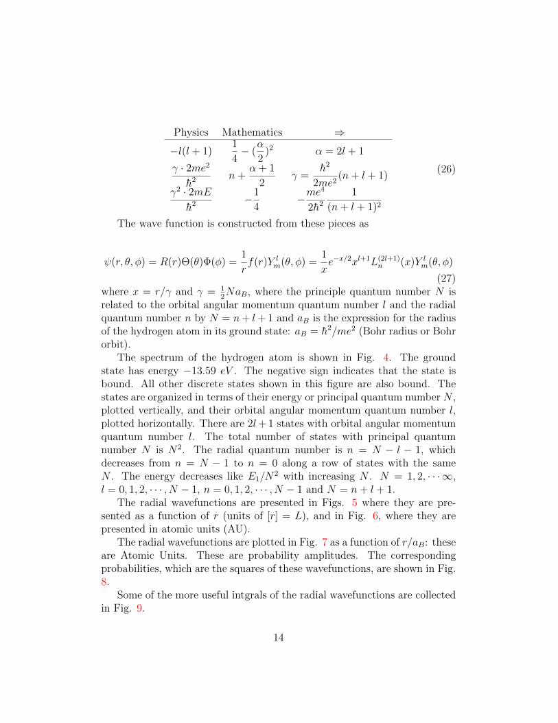
The spectrum of the hydrogen atom is shown in Fig. 4. The groundstate has energy −13.59 eV . The negative sign indicates that the state isbound. All other discrete states shown in this figure are also bound. Thestates are organized in terms of their energy or principal quantum number N ,plotted vertically, and their orbital angular momentum quantum number l,plotted horizontally. There are 2l+ 1 states with orbital angular momentumquantum number l. The total number of states with principal quantumnumber N is N2. The radial quantum number is n = N − l − 1, whichdecreases from n = N − 1 to n = 0 along a row of states with the sameN . The energy decreases like E1/N

2 with increasing N . N = 1, 2, · · ·∞,l = 0, 1, 2, · · · , N − 1, n = 0, 1, 2, · · · , N − 1 and N = n+ l + 1.

The radial wavefunctions are presented in Figs. 5 where they are pre-sented as a function of r (units of [r] = L), and in Fig. 6, where they arepresented in atomic units (AU).

The radial wavefunctions are plotted in Fig. 7 as a function of r/aB: theseare Atomic Units. These are probability amplitudes. The correspondingprobabilities, which are the squares of these wavefunctions, are shown in Fig.8.

Some of the more useful intgrals of the radial wavefunctions are collectedin Fig. 9.

14

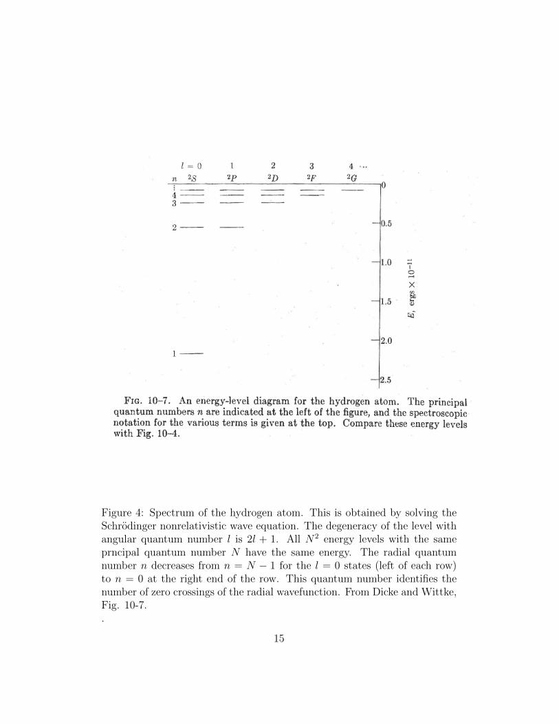
Figure 4: Spectrum of the hydrogen atom. This is obtained by solving theSchrodinger nonrelativistic wave equation. The degeneracy of the level withangular quantum number l is 2l + 1. All N2 energy levels with the sameprncipal quantum number N have the same energy. The radial quantumnumber n decreases from n = N − 1 for the l = 0 states (left of each row)to n = 0 at the right end of the row. This quantum number identifies thenumber of zero crossings of the radial wavefunction. From Dicke and Wittke,Fig. 10-7..

15

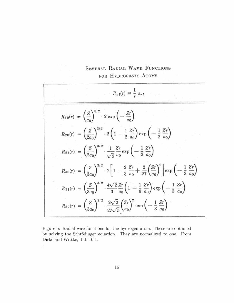
Figure 5: Radial wavefunctions for the hydrogen atom. These are obtainedby solving the Schrodinger equation. They are normalized to one. FromDicke and Wittke, Tab 10-1..

16

Figure 6: Radial wavefunctions of the hydrogen atom, expressed in terms ofatomic units. From Condon and Shortley, Table 15.

17

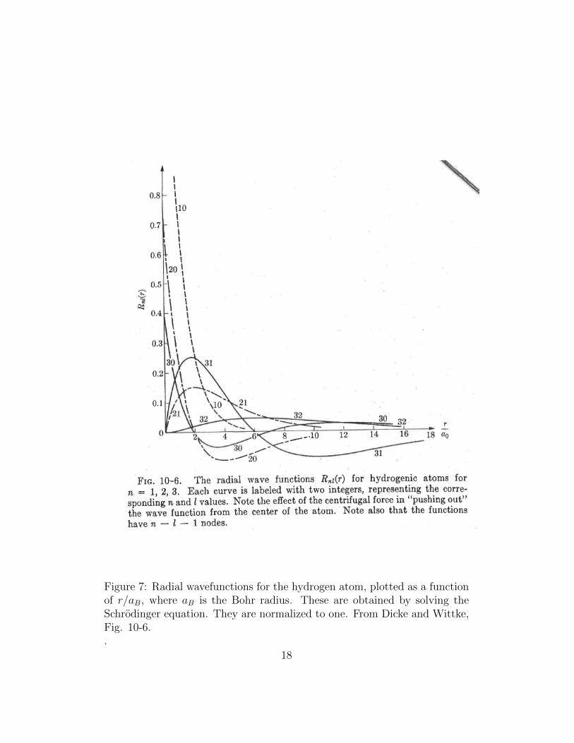
Figure 7: Radial wavefunctions for the hydrogen atom, plotted as a functionof r/aB, where aB is the Bohr radius. These are obtained by solving theSchrodinger equation. They are normalized to one. From Dicke and Wittke,Fig. 10-6..

18

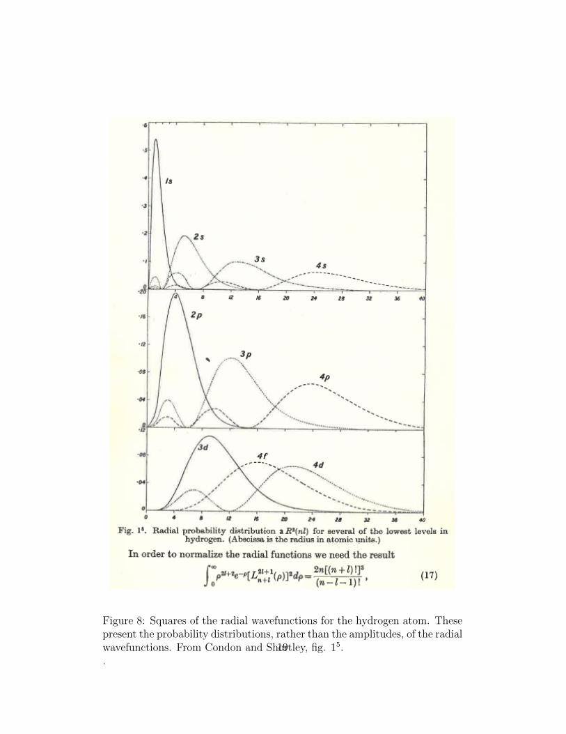
Figure 8: Squares of the radial wavefunctions for the hydrogen atom. Thesepresent the probability distributions, rather than the amplitudes, of the radialwavefunctions. From Condon and Shortley, fig. 15..

19

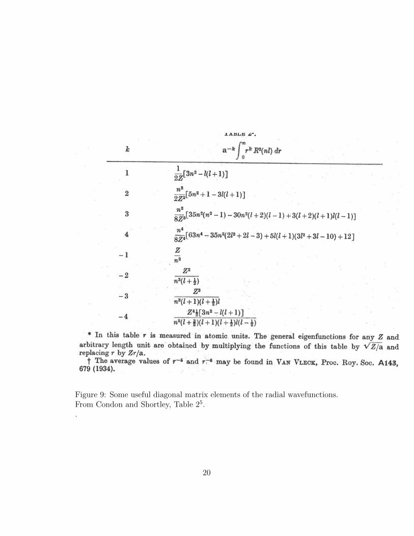
Figure 9: Some useful diagonal matrix elements of the radial wavefunctions.From Condon and Shortley, Table 25..

20

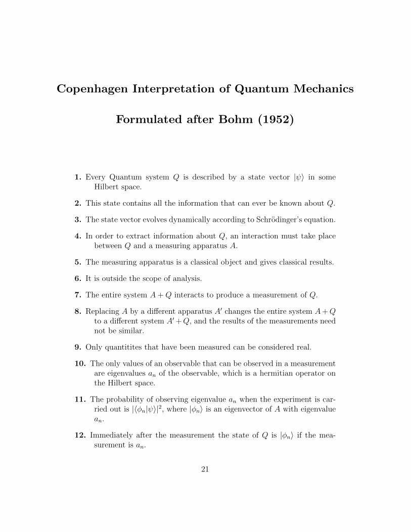
Copenhagen Interpretation of Quantum Mechanics

Formulated after Bohm (1952)

1. Every Quantum system Q is described by a state vector |ψ〉 in someHilbert space.

2. This state contains all the information that can ever be known about Q.

3. The state vector evolves dynamically according to Schrodinger’s equation.

4. In order to extract information about Q, an interaction must take placebetween Q and a measuring apparatus A.

5. The measuring apparatus is a classical object and gives classical results.

6. It is outside the scope of analysis.

7. The entire system A+Q interacts to produce a measurement of Q.

8. Replacing A by a different apparatus A′ changes the entire system A+Qto a different system A′+Q, and the results of the measurements neednot be similar.

9. Only quantitites that have been measured can be considered real.

10. The only values of an observable that can be observed in a measurementare eigenvalues an of the observable, which is a hermitian operator onthe Hilbert space.

11. The probability of observing eigenvalue an when the experiment is car-ried out is |〈φn|ψ〉|2, where |φn〉 is an eigenvector of A with eigenvaluean.

12. Immediately after the measurement the state of Q is |φn〉 if the mea-surement is an.

21

Remarks:

2. This philosophical point is not universally shared.

4. “Measuring apparatus” remains undefined.

5. It is claimed that von Neumann formulated things so the measuring appa-ratus could also be quantum mechanical. In view of his failures (Bohm’shidden variables theory is a counterexample to his “proof” that hiddenvariables theories are impossible; the laser is a counterexample to hisand Bohr’s adamant claims that masers/lasers violate the uncertaintyrelations and are therefore impossible), I cannot give credance to thisclaim.

6. This is a cop out.

8. Complementarity!

9. Einstein, Schrodinger have difficulty with this.

11. Born’s probabilistic interpretation.

12. Collapse of the wavefunction. There is no theory for this.

Some Questions:

1. What is the origin and meaning of the uncertainty relations? Or moregenerally of the noncommutativity of observables?

2. Where is the boundary in A+Q?

3. How does the apparatus force the “collapse of the wavefunction” |ψ〉 →|φn〉 during a measurement?

22

“Newtonian Formulation” of Copenhagen Interpretation

Definition of Coordinate System: The playing field on which QuantumMechanics takes place is a Hilbert space. A quantum system Q isrepresented by a state vector |ψ〉 in this Hilbert space, or more generallyby a density operator ρ on this space. Observables are represented byhermitian operators acting on this space.

Dynamics: The state |ψ〉 or ρ representing a quantum system evolves underthe Schrodinger equation.

Action and Reaction — Measurement: The quantum systemQ and theapparatus A measuring the value of an observable interact with eachother during a measurement. Q acts on A to produce an eigenvaluean with probability |〈φn|ψ〉|2, where |φn〉 is a normalized eigenvectorof the hermitian operator A with eigenvalue an. A back-reaction of Aon Q guarantees that Q is in the eigenstate |φn〉 immediately after themeasurement.

23