Quantum Mechanics

B. Sathiapalan

July 7, 2004

1 Course Contents

1. Free Particle: (9 lectures)

(a) Schroedinger Equation, Hamiltonian, Commutation Relations,Wave functions, Probability Interpretation, Currents, Measure-ment, Plane waves, Normalization, Boundary conditions, Dis-crete Space and Regularization, delta function, Wave packets,group velocity. (1 1/2 lectures)

(b) Postulates of QMech, Bra-ket notation, Fourier Transform, Vec-tor Space. (1 1/2 )

(c) Matrices, Hermitian, Unitary, Tensor Product, Projection Oper-ator.(1)

(d) Schroedinger and Heisenberg Representation, Evolution Opera-tor.(1)

(e) Feynman Path Integral.(2)

(f) Density Operator, Quantum Statistical Mechanics. (2)

2. Spin-1/2 system:(3 lectures)

(a) Stern Gerlach, Illustrating q mech., Atom in a magnetic field,Dynamics of two level systems. (2)

(b) Quantum Computer.(1)

3. Rotation Group: (4 lectures)

(a) Symmetries and Conservation Laws, Lie Groups, Rotation, Lorentz,Poincare, Global and local invariances (gauge invariance).(2)

1

(b) Spin and Orbital Angular Momentum, Spherical harmonics.(2)

(c) Discrete Symmetries:C,P,T. (1)

4. Harmonic Oscillator: (4 lectures)

(a) Path Integral treatment. (2)

(b) Anharmonic Oscillator.(1/2)

(c) Coherent states.(1/2)

(d) Introduction to field theory.(1)

5. Perturbation Theory: (5 lectures)

(a) Time Independent (Degenerate and Non-degenerate Pert. The-ory).(1)

(b) Time Dependent Perturbation Theory, Sinusoidal perturbations,Fermi Golden Rule.(1)

(c) Scattering Theory.(3)

6. Interaction of Charged Particles:(11 lectures)

(a) Hamiltonian and Lagrangian, Gauge Invariance. (1/2)

(b) Bohm-Aharanov Effect.

(c) Path Integral.(1 1/2)

(d) Hydrogen Atom, Diatomic Molecule. (2)

(e) Atom in an Electric and Magnetic Field, NMR. (2)

(f) Fine and Hyperfine Structure, Lamb Shift.(1)

(g) Electron in a Magnetic Field. , Landau levels, QHE (Q HallEffect).(1)

(h) QED, Scattering, Dipole Radiation.(3)

7. Dirac Equation and Klein Gordon Equation.(4 lectures)

Text Books:

1. Cohen-Tannoudji....

2. Landau and Lifshitz....

3. Feynman and Hibbs ....

2

These notes foloow these books quite closely.Grading Policy:

Homework : 30 %Mid-term examination: : 20 %Final Examination: : 50 %Total : 100 %

Other points:

1. Homework assignments will be given out once a week and will be dueback in exactly one week. Homeworks handed in late will not begraded. You may consult with each other on the homework problems(indeed this is a very good thing), but the final solution should beyours. You may also be asked occasionally to work out problems onthe board.

2. Basic knowledge of quantum mechanics is assumed. The aim of thecourse is to extend your formalistic and mathematical skills and alsodevelop physical intuition.

3. Although text books have been specified we will not follow the orderof presentation of any particular book. In terms of material Cohen-Tannoudji will be followed quite closely. For path integrals Feynmanand Hibbs. The quasi-classical approximation is taken from Landau-Lifshitz. There are many other good books, such as those by Dirac,Schiff, Sakurai...

3

2 Free Particle

2.1 Basics

In classical mechanics a free particle is described by specifying its mass m,position x and momentum p. The Hamiltonian is given by

H =p2

2m(1)

In Heisenberg’s formulation this equation continues to be true butx, p are non-commuting operators that satisfy

[x, p] = ih (2)

Dimensions: xp has dimensions L2T−1M - dimensions of angular mo-mentum. This is also ML2T−2T which is energy × time. This has di-mensions of “action”. In q.mech. we often use units where h = 1. ThenE ≈ T−1. Also P ≈ L−1. Then action can be said to be dimensionless.In relativistic sytems it is common to set c = 1 (c=vel. of light). (Soh = c = 1). L ≈ T ≈ E−1 ≈ P−1 ≈ M−1. Thus in these units, p,E,m allhave dimensions of 1/length. However for non-relativistic quantum mechwe usually keep the constants.

(H.W: Show that e2

4πε0hcis dimensionless. What is it’s value? Can you

define something analogous using the other important constants in nature:G gravitaional constant? Should the fundamental constants in nature bedimensionful or dimensionless? What if we had a universe where h hastwice its present value, and all other (dimensionless nos.) are the same.What would be different? Think about these things.)

e = 1, 6× 10−19 Coul

h = 1.05× 10−34 J − s

c = 3× 108 m/s

14πε0

= 8.98× 109 Nm2

coul2

G = 6.6× 10−11 Nm2

kg2

In this formulation the possible values that can result when momentumis measured(what does this mean??) are the eigenvalues of the operator

4

p. Same for x. Operators can be represented by matrices. Eigenvalues ofH are thus the measured values of energy. In particular at the end of ameasurement the particle has that measured value i.e. it is in an eigenstateof that operator. As x and p do not commute, it follows that the particlecannot be simultaneously an eigenstate of both. Therefore if it has a precisevalue of momentum, it cannot have a precise value of position, and viceversa. This observation is embodied in the “Heisenberg UncertaintyRelation”

∆x∆p ≥ h

2(3)

In the Heisenberg formalism one has to diagonalise matrices.(Do they know Fourier Transforms?) This is trivially a consequence of

the mathematical properties of FT.In the Schroedinger formulation one has to solve a linear differential

equation:

Hψ = ih∂ψ

∂t(4)

where H is a linear differential operator. It is equal to − 12m

∂2

∂x2 From study-ing differential equations we know that this also reduces to an eigenvalueproblem. Thus the space of solutions of Schroedinger’s equation forms avector space on which H, p, x can be represented as (infinite dimensional,why?) matrices. These matrices satisfy Heisenberg’s commutation relations.

In a nutshell these are the two (equivalent) descriptions of quantummechanics discovered in the 1920’s. R.P. Feynman discovered (1940?)another formulation called the path integral formulation. We will discussthis soon. This idea is used a lot in Quantum Field Theory.

Schroedinger’s formulation is more convenient for Non-relativistic QM.Things you should know:1. The wave function represents what? Born’s probability interpretation:

dP ∝| ψ |2 dx1.1. Given a wave function, physical quantities that can be calculated

are expectation values of operators such as x, p, .. and functions thereof:∫ +∞

−∞ψ∗Oψdx =< O >

2. Normalization :∫+∞−∞ | ψ |2 dx = 1. This is a physical requirement

and constrains the solutions of SE.3. In this representation p is represented by −ih ∂

∂x .

5

3.1. Proof of uncertainty reln.:Consider for α real:∫ +∞

−∞| αxψ + ∂

∂xψ |2 dx ≥ 0

The three terms are:

α2∫x2 | ψ |2 dx = α2(∆x)2

∫| ∂∂xψ |

2 dx =(∆p)2

h2

∫αx(ψ ∂

∂xψ∗ + ψ∗ ∂∂xψ)dx = −α

They add up to

α2(∆x)2 − α+(∆p)2

h2 ≥ 0

This means the discriminant has to be≤ 0. So

1− 4(∆x)2(∆p)2

h2 ≤ 0

This gives

(∆x)(∆p) ≥ h

2

4. The eigenfns of p are Aeikx and have ev hk. “plane waves”5. These plane waves are not normalizable.

∫+∞−∞ | ψ |2 dx = ∞. Dirac

introduced a “delta function” to deal with these. The Dirac Delta Functionδ(x) is zero everywhere except at x = 0 where it is infinite. It also satisfies∫dxδ(x) = 1. And

∫dxf(x)δ(x) = f(0). Using this notation one can show

that (HW)∫+∞−∞ | ψ |2 dx =| A |2 2πδ(0). (for plane wave states). These

are called “plane wave normalizable”. Although these states are not allowedstrictly speaking we will use them as an approximation and for practicalconvenience.

Another way to deal with plane waves is to put it in a box:Size L. So if Ψ(x) = Aikx is plane wave, then |A|2 = 1√

L. This is

infrared regularization. What is the smallest value: Depends on bc.If we have standing waves, then we have states with sin kx and k = nπ

L .(Periodic?)

6

Ultraviolet gularizatipon assume k has a max. As in a crystal withspacing a. k ≤ 2π

a . And Na = L. So k takes N values.dx→

∑Nn=1 a. dk →

∑Nm=1

2πL . Try evaluationg

∫dxeikx and

∫dk∫dxeikx

and figure out properties of delta-function.6.Probability density of finding a particle in such a state (=constant)7. Probability current:

Jx =h

2im[ψ∗∂xψ − c.c.] =

hk

m︸︷︷︸velocity

| A |2︸ ︷︷ ︸number density

(5)

8. Current Conservation ∂xJx − ∂tJt = 0 where Jt = ψ∗ψ = numberdensity.

9. States havind a definite time dependence e−iEt satisfy the time inde-pendent SE Hψ = Eψ. For plane wave states clearly E = (hk)2

2m .10. We usually require E to be real. what if it is not? Calculate ∂t(ψ∗ψ).11. Continuous versus discrete E. Confining potentials and bound

states. Particle in a box. HW.12. Prove current conservation using SE. Starting with − h2∂2ψ

2m∂x2 = i h∂ψ∂twe get (multiply by ψ∗, integrate by parts and subtract c.c) −∂xJx on theLHS and i∂t(ψ∗ψ) on the RHS. QED.

12. HW problem with particle leaking out of a box.13. Given a wave function, physical quantities that can be calculated

are expectation values of operators such as x, p, .. and functions thereof:∫ +∞

−∞ψ∗Oψdx =< O >

14.For a plane wave what is < x >,< x2 >? What does it mean?15. Given the above, how does one construct a classical looking particle?

ANS “wave packet”. Superpose different harmonics: Draw. eg ψ(x) =

Ae−(x−vt)2

2b2 . Do you know how to fix A? This represents a particle movingalong the trajectory x = vt. At least initially. After some time? calculate!

16. Group velocity is dωdk is k

m . But what is k? ψ is peaked around somek. Consider the wave fn.

ψ = A

∫dkeikxe−

b2(hk−mv)2

2 e−ih2k2t2m (6)

This represents a superposition of plane waves of momentum hk and theappropriate time dependence. k peaked around mv. Do the integral. Set

7

h = 1. The exponent is:

−k2(b2

2+ i

t

2m) + k(b2mv + ix)− m2v2b2

2

= −(b2

2+ i

t

2m)(k − (b2mv + ix)

(b2 + i tm))2 +

(b2mv + ix)2

2(b2 + i tm)− m2v2b2

2

After doing the k integral we are left with a term in the exponent:

(b2mv + ix)2

2(b2 + i tm)− m2v2b2

2

We expand this for large m but small mb to get

ψ ≈ e−(x−vt)2

2b2−itmv2

2+imvx (7)

We can also calculate | ψ | by adding to the exponent its c.c. to get

| ψ |≈ e− b2(x−vt)2

(b4+ t2

m2 ) (8)

This clearly represents a ‘semi-classical’ wave function of a particle mov-ing along a trajectory with vel v. The t and x dependences give the classicalenergy and momentum respectively.

The Feynman Path Integral (FPI) approach is best suited to demonstratethis. Later.

2.2 Postulates of Q.M.

1. The space of allowed “wave-fns” is a vector space over complex nos.(Hilbert space). The wave fns have to be square integrable and smoooth.

i) Superposition: ψ = a1ψ1 + a2ψ2, a1, a2 ∈ C is also a physical state.ii)Scalar product

∫d3rφ∗(r)ψ(r) =< φ | ψ > has the following props:

a)< φ | ψ >∗=< ψ | φ >b)Linear < φ | a1ψ1 + a2ψ2 >= a1 < φ | ψ1 > +a2 < φ | ψ2 >c)anti linear < a1ψ1 + a2ψ2 | φ >= a∗1 < ψ1 | φ > +a∗2 < ψ2 | φ >d) Norm < φ | φ >=

∫d3rφ∗φ > 0 and is =0 iff φ = 0. 2.Dirac’s

Notation:| ψ > represents a state. Inner product of | ψ > and | φ > is denoted by

< φ | ψ >

8

Thusψ(r) ↔| ψ >

“ket” ∫d3rφ∗(r)ψ(r) ↔< φ | ψ >

Dual space: The space of linear functionals:defn of lin fnl: χ is a linear fnl ⇒ it assigns a complex no. to every ket

| ψ >.χ(| ψ >) = c

The space of χ’s is the dual vector space.Linear i.e. aχ1(| ψ >) + bχ2(| ψ >) = aχ1 + bχ2(| ψ >)Hilbert space and its dual are isomorphic. (Except for plane wave states!)A particular linear functional ψdual can be associated with a ket | ψ >

by:ψdual(| φ >) ≡< ψ | φ >

This defines the bra < φ |≡ φdual.3. Basis vectors: | ei > i = 1, N for an N dim space. Completenes.

Discrete and continuous.Orthonormal:< en | em >= δnm or < e(λ) | e(λ′) >= δ(λ− λ′)Thus usual wave fn ψ(r) =< r | ψ >

| ψ >=∫d3rψ(r) | r >

< r | r >= δ(0) = ∞ not normalizable.Momentum basis:

ψ(r) =∫

d3p

(2π)3ψ(p)eip.r

“Fourier transform”

ψ(p) =∫d3re−ip.rψ(r)

Check .Define | p > by ψ(p) =< p | ψ >. and

| ψ >=∫

d3p

(2π)3ψ(p) | p >

9

This requires < p | ∂′ >= (2π)3δ3(p− p′)

| ψ >=∫d3r

∫d3p

(2π)3ψ(p) | r >

=∫

d3p

(2π)3ψ(p)

∫d3reip.r | r >︸ ︷︷ ︸

|p>

Thus < r | p >= eip.r.Thus inserting

∫ d3p(2π)3

| p >< p | or∫d3r | r >< r | is equivalent to FT.

4. Operators: Linear operator: A | ψ >=| φ > and correspondinglyAψ(r) = φ(r) where A is a differential operator.

Aψ(r) =< r | A | ψ >=∫d3r′ < r | A | r′ > ψ(r′)

< r | A | r′ > are matrix elements. Operators are represented by matrices.Discrete or continuous depends on basis.

eg A is -id/dx what is A?

−id/dxψ(x) =∫dx′id/dx′δ(x− x′)ψ(x′)

=∫dx′id/dx′ < x | x′ > ψ(x′)

=∫dx′[< x | id/dx′ | x′ >]ψ(x′)

< x | A | x′ >=< x | id/dx′ | x′ >= id/dx′δ(x− x′)

. (Note the sign change)

< p | A | p′ >=∫dxp′ei(p

′−p)x = 2πδ(p′ − p)p′

5. Hermiticity: A = A†

< χ | Aψ >∗=< ψ | A† | χ >

∫dx(χ∗Aψ)∗ =

∫dxψ∗A†χ =

∫dx(Aψ)∗χ

10

eg A = d/dx:∫(χ∗(x)dψ/dx)∗ =

∫dψ∗/dxχ(x) = −

∫dxψ∗dχ/dx

Note - sign. We have “integrated by parts”. (What boundary conditionsare required?) Thus A† here is −d/dx. Thus it is anti-Hermitian. Thus i ddxis Hermitian.

6. Eigenvalues and eigenvectors.If A|ψn >= an|ψn > then an is an eigenvalue and |ψn > is an eigen

vector.

2.3 Matrices

If ei ≈ |i > are a orthonormal basis then the matrix Aij =< i|A|j > is thematrix representaion of the operator A. Thus

A|j >=∑k

Akj |k >

< i|A|j >=∑k

Akj < i|k >= Aij

Thus if |ψ >=∑an|n > the column vector (an) represents the state

|ψ >. ThenA|ψ >=

∑i

A|i >< i|ψ >=∑i

aiA|i >

=∑i

ai∑j

|j >< j|A|i >

=∑j

(∑i

Ajiai)|j >

So the numbers∑iAjiai represents A|ψ >.

Diagonal rep of matrix : Choose a (orthonormal) basis consisting ofeigenvectors ofA. In this basisA is a diagonal matrix: A = diag(a1, a2, a3...aN ).Then A = A† implies that the eigevalues are real. Physical (i.e. experimen-tally measurable) quantities must be represented by Hermitian matrices.eg. energy, momentum,...Hermitian means real symmetric, or imaginaryantisymmetric. eg Pauli matrices.

Unitary matrices: UU † = U †U = I.They are important - they preserve norm:

< Uψ|Uψ >=< ψ|U †U |ψ >=< ψ|ψ >

11

Det(UU †) = DetUDetU † = |DetU |2 = 1

So DetU = ±1. If we diagonalise U then since U−1 = U † = U∗ the diagonalelements must be of the form eiθn where θn is real.

Thus U = eiA where A is hermitian. (iA is anti Hermitian).If A is small, the U = 1+iA, and U † = 1−iA. A Unitary transformation

isUFU † = (1 + iA)F (1− iA)

= F + i[A,F ]

ThusδF = i[A,F ]

is the form of the infinitesimal transformation. eg eiεPh is a translation by ε.

δF = iε[P

h, F ] = iε(−idF

dx

= εdF

dx

2.4 Tensor Products

V1, V2 are two vector spaces. The tensor product is a vector space V1 ⊗ V2.If |e1i >, i = 1−N1, |e2j >, j = 1−N2 are the bases of V1, V2, then the N1N2

states |e1i > ⊗|e2j > are the basis states of V1 ⊗ V2.eg |px, py, pz > actually is a state in the tensor product space |px >

⊗|py > ⊗|pz >. Similarly, multiparticle states.1.

λ[|φ1 > ⊗|χ2 >] = λ[|φ1 >]⊗ |χ2 >= |φ1 > ⊗λ[|χ2 >]

2.|φ1 > ⊗[|χ1 > +|χ2 >] = |φ1 > ⊗|χ1 > +|φ1 > ⊗|χ2 >]

3. If |φ1 >=∑N1n=1 an|e1n > and |χ1 >=

∑N2m=1 bm|e2m >, then

|φ1 > ⊗|χ1 >=∑N1n=1

∑N2m=1 anbm︸ ︷︷ ︸

N1+N2

|e1n.⊗ |e2m >

4. But the general state is |Ψ >=∑N1n=1

∑N2M=1 cn,m︸︷︷︸

N1N2

|e1n > ⊗|e2m >

5. Scalar product |φ1 > ⊗|χ1 > and |φ2 > ⊗|χ2 >

12

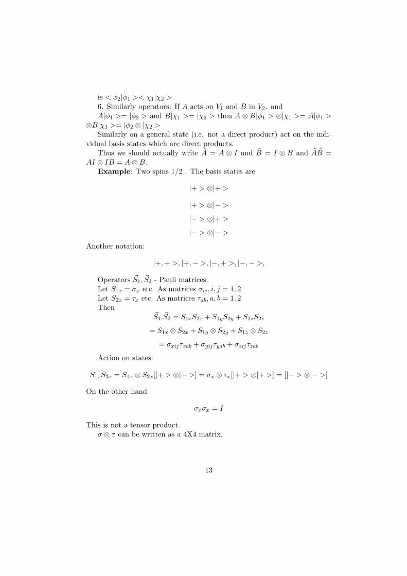
is < φ2|φ1 >< χ1|χ2 >.6. Similarly operators: If A acts on V1 and B in V2. andA|φ1 >= |φ2 > and B|χ1 >= |χ2 > then A ⊗ B|φ1 > ⊗|χ1 >= A|φ1 >

⊗B|χ1 >= |φ2 ⊗ |χ2 >Similarly on a general state (i.e. not a direct product) act on the indi-

vidual basis states which are direct products.Thus we should actually write A = A ⊗ I and B = I ⊗ B and AB =

AI ⊗ IB = A⊗B.Example: Two spins 1/2 . The basis states are

|+ > ⊗|+ >

|+ > ⊗|− >

|− > ⊗|+ >

|− > ⊗|− >

Another notation:

|+,+ >, |+,− >, |−,+ >, |−,− >,

Operators ~S1, ~S2 - Pauli matrices.Let S1x = σx etc. As matrices σij , i, j = 1, 2Let S2x = τx etc. As matrices τab, a, b = 1, 2Then

~S1.~S2 = S1xS2x + S1yS2y + S1zS2z

= S1x ⊗ S2x + S1y ⊗ S2y + S1z ⊗ S2z

= σxijτxab + σyijτyab + σzijτzab

Action on states:

S1xS2x = S1x ⊗ S2x[|+ > ⊗|+ >] = σx ⊗ τx[|+ > ⊗|+ >] = [|− > ⊗|− >]

On the other hand

σxσx = I

This is not a tensor product.σ ⊗ τ can be written as a 4X4 matrix.

13

2.5 CSCO

Complete Set of Commuting Observables: How do you specify a state com-pletely?

Let the eigenvectors of A be |an >, i.e. A|an >= an|an >. There maybe many of these. So label by another index: |an, i >, i : 1−Nn. How doesone label them? Use another observable B such that [A,B] = 0. B will notchange A eigenvalue. So

B|an, i >=∑j

bij |an, j >

Thus B is block diagonal. Draw. Let us diagonalise B in each block. Soinstead of i use bm, Thus the states are labelled by |an, bm >,m : 1−Nb. IfNb = Nn then we have a distinct eigenvalue for each state. If Nb < Nn

then then we have many states with same values an, bm. Thus we callthem |an, bm, k > where k : 1 − Nn,m. Find another operator C such that[A,C] = [B,C] = 0. This is block diagonal in the block labelled by an, bm.Diagonalise it. Let the ev be cp. If all ev are distinct we are done. Otherwisekeep going. In this way we get a CSCO: A,B,C,D, ... and a set of labelsthat uniquely specify the state |an, bm, cp, dq, ... >. The set is not unique.

eg Plane waves in three dimensions.

2.6 Projection Operators

P is a projection operator if P 2 = P . Eigenvalues are 1,0.Projector into a state |ψ > is |ψ><ψ|√

<ψ|ψ>

2.7 Schroedinger, Heisenberg and Interaction Representa-tion

1.ψ(x, t) = e−

ihHtψ(x, 0) (9)

if H is time independent.2.

ψ(x, t) = Pe−ih

∫ t

0H(t′)dt′︸ ︷︷ ︸

EvolutionOperator

ψ(x, 0) (10)

if H is time dependent. P stands for “Path Ordering”.3. The evolution operator U(t, 0) is unitary if H is Hermitian. U(t, 0) =

U(t, t1)U(t1, 0).

14

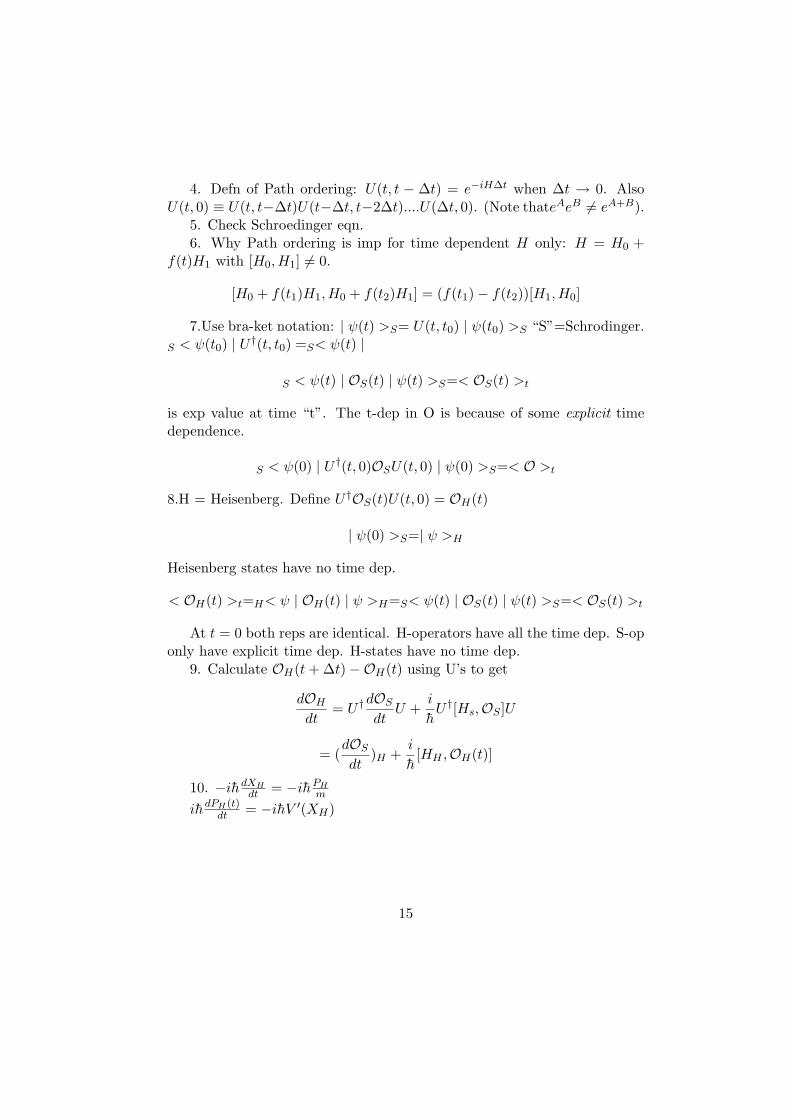
4. Defn of Path ordering: U(t, t − ∆t) = e−iH∆t when ∆t → 0. AlsoU(t, 0) ≡ U(t, t−∆t)U(t−∆t, t−2∆t)....U(∆t, 0). (Note thateAeB 6= eA+B).

5. Check Schroedinger eqn.6. Why Path ordering is imp for time dependent H only: H = H0 +

f(t)H1 with [H0,H1] 6= 0.

[H0 + f(t1)H1,H0 + f(t2)H1] = (f(t1)− f(t2))[H1,H0]

7.Use bra-ket notation: | ψ(t) >S= U(t, t0) | ψ(t0) >S “S”=Schrodinger.S < ψ(t0) | U †(t, t0) =S< ψ(t) |

S < ψ(t) | OS(t) | ψ(t) >S=< OS(t) >t

is exp value at time “t”. The t-dep in O is because of some explicit timedependence.

S < ψ(0) | U †(t, 0)OSU(t, 0) | ψ(0) >S=< O >t

8.H = Heisenberg. Define U †OS(t)U(t, 0) = OH(t)

| ψ(0) >S=| ψ >H

Heisenberg states have no time dep.

< OH(t) >t=H< ψ | OH(t) | ψ >H=S< ψ(t) | OS(t) | ψ(t) >S=< OS(t) >t

At t = 0 both reps are identical. H-operators have all the time dep. S-oponly have explicit time dep. H-states have no time dep.

9. Calculate OH(t+ ∆t)−OH(t) using U’s to get

dOHdt

= U †dOSdt

U +i

hU †[Hs,OS ]U

= (dOSdt

)H +i

h[HH ,OH(t)]

10. −ihdXHdt = −ihPH

m

ihdPH(t)dt = −ihV ′(XH)

15

2.8 Path Integral

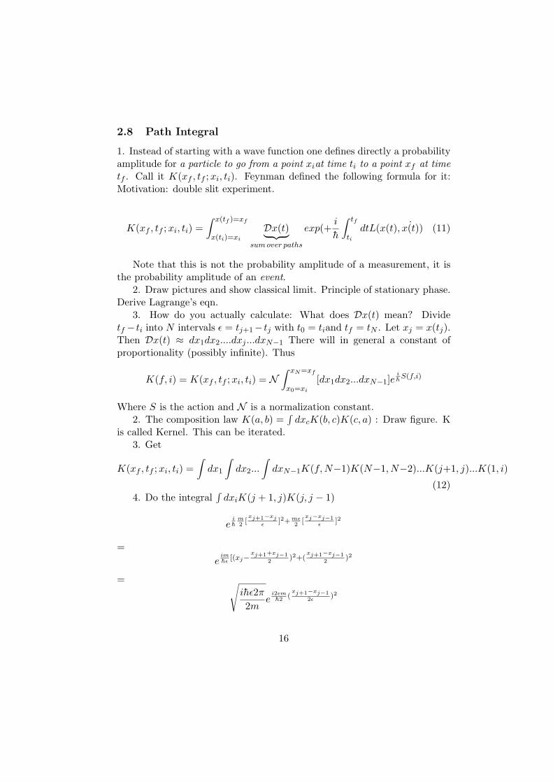
1. Instead of starting with a wave function one defines directly a probabilityamplitude for a particle to go from a point xiat time ti to a point xf at timetf . Call it K(xf , tf ;xi, ti). Feynman defined the following formula for it:Motivation: double slit experiment.

K(xf , tf ;xi, ti) =∫ x(tf )=xf

x(ti)=xi

Dx(t)︸ ︷︷ ︸sumover paths

exp(+i

h

∫ tf

ti

dtL(x(t), ˙x(t)) (11)

Note that this is not the probability amplitude of a measurement, it isthe probability amplitude of an event.

2. Draw pictures and show classical limit. Principle of stationary phase.Derive Lagrange’s eqn.

3. How do you actually calculate: What does Dx(t) mean? Dividetf − ti into N intervals ε = tj+1− tj with t0 = tiand tf = tN . Let xj = x(tj).Then Dx(t) ≈ dx1dx2....dxj ...dxN−1 There will in general a constant ofproportionality (possibly infinite). Thus

K(f, i) = K(xf , tf ;xi, ti) = N∫ xN=xf

x0=xi

[dx1dx2...dxN−1]eihS(f,i)

Where S is the action and N is a normalization constant.2. The composition law K(a, b) =

∫dxcK(b, c)K(c, a) : Draw figure. K

is called Kernel. This can be iterated.3. Get

K(xf , tf ;xi, ti) =∫dx1

∫dx2...

∫dxN−1K(f,N−1)K(N−1, N−2)...K(j+1, j)...K(1, i)

(12)4. Do the integral

∫dxiK(j + 1, j)K(j, j − 1)

eih

m2

[xj+1−xj

ε]2+mε

2[xj−xj−1

ε]2

=e

imhε

[(xj−xj+1+xj−1

2)2+(

xj+1−xj−12

)2

= √ihε2π2m

ei2εmh2

(xj+1−xj−1

2ε)2

16

This is clearly proportional to K(j+ 1, j− 1). The factor in square rootis the normalization factor. If we use the Gaussian normalization factor foreach of the unit K’s , i.e.

√m

2πεhi , we get the final result

√m

2π2εhie

i2εmh2

(xj+1−xj−1

2ε)2

which has the correct normalization.Clearly this process can be iterated to replace 2ε by Nε = tf − ti. Thus

K(xf , tf ;xi, ti) =√

m

2π(tf − ti)hie

i(tf−ti)m

h2((xf−xi)

(tf−ti))2

(13)

5. Relation to wave functions - evolution operator.

ψ(xf , tf ) = e−i∫ tf

tiHdt

ψ(xi, ti) =∫K(xf , tf ;xi, ti)ψ(xi, ti)dxi (14)

5.5) Expansion of K(xf , tf ;xi, ti) in terms of wave functions

K(xf , tf ;xi, ti) =∑n

ψn(xf )ψ∗n(xi)e−i

En(tf−ti)

h

6. Derivation of Schroedinger’s eqn.Consider infinitesimal evolution from t to t+ ε. The evolution operator

is

K(xf , tf ;xi, ti) =∫ x(tf )=xf

x(ti)=xiDx(t)︸ ︷︷ ︸

sumover paths

exp(+ ih

∫ tfti dtL(x(t), ˙x(t))

We set tf = ti + ε to get

ψ(xf , ti+ε) =∫ x(ti+ε)=xf

x(ti)=xi

Dx(t)︸ ︷︷ ︸sumover paths

exp(i

h

∫ ti+ε

ti

dtL(x(t), ˙x(t))ψ(xi, ti)dxi

For infinitesimal evolution

ψ(xf , ti + ε) = N∫e

ih

m2ε[

xf−xiε

]2ψ(xi, ti)dxi

17

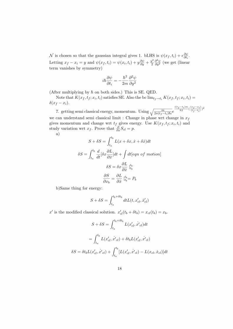
N is chosen so that the gaussian integral gives 1. bLHS is ψ(xf , ti) + ε ∂ψ∂ti .

Letting xf − xi = y and ψ(xf , ti) = ψ(xi, ti) + y ∂ψ∂y + y2

2∂2ψ∂y2

(we get (linearterm vanishes by symmetry)

ih∂ψ

∂ti= − h2

2m∂2ψ

∂y2

(After multiplying by h on both sides.) This is SE. QED.Note thatK(xf , tf ;xi, ti) satisfies SE. Also the bc limtf→ti K(xf , tf ;xi, ti) =

δ(xf − xi).

7. getting semi classical energy, momentum. Using√

m2π(tf−ti)hie

i(tf−ti)m

h2((xf−xi)

(tf−ti))2

we can understand semi classical limit : Change in phase wrt change in xfgives momentum and change wrt tf gives energy. Use K(xf , tf ;xi, ti) andstudy variation wrt xf . Prove that ∂

∂xScl = p.a)

S + δS =∫ tb

taL(x+ δx, x+ δx)dt

δS =∫ tb

ta

d

dt[δx

∂L

∂x]dt+

∫dt[eqn of motion]

δS = δx∂L

∂x|tbtb

∂S

∂xb=∂L

∂x|tbtb= Pb

b)Same thing for energy:

S + δS =∫ tb+δtb

tadtL(t, x′cl, x

′cl)

x′ is the modified classical solution. x′cl(tb + δtb) = xcl(tb) = xb.

S + δS =∫ tb+δtb

taL(x′cl, x′cl)dt

=∫ tb

taL(x′cl, x′cl) + δtbL(x′cl, x′cl)

δS = δtbL(x′cl, x′cl) +∫ tb

ta[L(x′cl, x′cl)− L(xcl, xcl)]dt

18

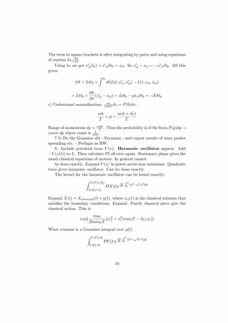
The term in square brackets is after integrating by parts and using equationsof motion δxcl δLδx .

Using bc we get x′cl(tb) + x′clδtb = xcl. So x′cl − xcl = −x′clδtb. All thisgives:

δS = Lδtb +∫ tb

dt[L(t, x′cl, x′cl)− L(t, xcl, xcl)

= Lδtb +∂L

∂x(x′cl − xcl) = Lδtb − pxclδtb = −Eδtb.

c) Understand normalization: m2πhT dx = P (b)dx.

mb

T< p <

m(b+ dx)T

Range of momentum dp = mdxT . Thus the probability is of the form P (p)dp =

const dp where const is 12πh .

7.5) Do the Gaussian slit - Feynman - and repeat results of wave packetspreading etc. - Perhaps as HW.

8. Include potential term V (x). Harmonic oscillator approx. Add−V (x(t)) to L. Then calculate PI all over again. Stationary phase gives theusual classical equations of motion. In general cannot

be done exactly. Expand V (x) in power series near minimum. Quadraticterm gives harmonic oscillator. Can be done exactly.

The kernel for the harmonic oscillator can be found exactly:∫ X(T )=Xf

X(0)=Xi

DX(t)eim2h

∫ T

0(x2−ω2x2)dt

Expand X(t) = Xclassical(t)+ y(t), where xcl(t) is the classical solution thatsatisfies the boundary conditions. Expand. Purely classical piece give theclassical action. This is

exp imω

2hsinωT[(x2

f + x2i )cosωT − 2xfxi]

What remains is a Gaussian integral over y(t)∫ Y (T )=0

Y (0)=0DY (t)e

im2h

∫ T

0(Y 2−ω2Y 2)dt

19

Expand y(t) =∑n ansin(nπtT )

KE = T∑n

a2n

12(nπ

T)2

PE = T∑n

12a2nω

2

Do integral over an (Jacobian is a constant) : the integral is of the formeconsta

2n((nπ

T)2−ω2). The constant is independent of ω and has the same value

when ω = 0. This integral is const′ × (1− ω2T 2

n2π2 )−12 .Product over all n gives

( sinωTωT )−1/2. Comparing with free particle gives const′ = ( m2πihT )1/2.

The final result:

(mω

2πihsinωT)1/2exp imω

2hsinωT[(x2

f + x2i )cosωT − 2xfxi]

9. Do with forcing function. Only classical action will be different.10. Several degrees of freedom. K(xf , Xf , tf ;xi, Xi, ti). The conve-

nience of the formalism. Separable systems. S(x,X) = S1(x) +S2(X). Theconcept The final result:

(mω

2πihsinωT)1/2exp imω

2hsinωT[(x2

f + x2i )cosωT − 2xfxi]

9. Do with forcing function. Only classical action will be different.10. Several degrees of freedom. K(xf , Xf , tf ;xi, Xi, ti). The conve-

nience of the formalism. Separable systems. S(x,X) = S1(x) +S2(X). Theconcept of “integrating out” degrees of freedom. When would you want todo that: unobservables : eg ren group - effective actions, thermodynamicheat bath or the rest of the universe,

2.9 Statistical Mechanics and the Density Matrix

1.Elementary Quantum Stat Mech: Expectation value of an operator inequilibrium so that states are weighted with Boltzmann factor < A >=∑i piAi where pi = 1

Z e−βEi

Z The partition fn. Free energy.F (T, V,N)or E(S, V,N).2.Other infmn P (x)? Need the unintegrated form of the partition fn i.e.

density matrix.3. P (x) = 1

Z

∑i φ

∗i (x)φi(x)e

−βEi

20

Similarly

< A >=1Z

∑i

Aie−βEi

=1Z

∑i

φ∗i (x)Aφi(x)e−βEi =

1Z

∑i

< φi | A | φi > e−βEi

Defineρ(x′, x) =

∑i

φi(x′)φ∗i (x)e−βEi

ρ =∑i

| φi >< φi | e−βEi

=∑i

| φi >< φi |︸ ︷︷ ︸1

e−βH

= 1.e−βH

“Density Matrix”.

< A >=1ZTr[Aρ] =

∫dxAρ(x′, x)δ(x− x′)

where Z = Tr[ρ] =∫dxρ(x, x)

4. Consider

K(xf , tf ;xi, ti) =∑n

ψn(xf )ψ∗n(xi)e− i

hEn(tf−ti)

If we let i(tf − ti) = βh we have the density matrix!Thus can use path integral with ith replaced by u to evaluate ρ:

ρ(x′, x) = K(x′, βh;x, 0) =∫x(0)=x,x(βh)=x′

(exp−1h

∫ β

0h[m

2x2(u)+V (x)]du)Dx(u)

To calculate Z = Tr[ρ] set x′ = x and integrate over x, i.e. sum over allperiodic paths.

5. Density operator in general:a) Pure case : ρk =| ψk >< ψk |. Assume normalized. ρ2 = ρ. Trρ = 1.In terms of some energy eigenstates (say):| ψk >=

∑n cn | φn > with∑

n c∗ncn = 1. So

ρk =∑n,m

c∗ncm | φm >< φn |

21

Trρ = 1 clearly. Off diagonal elements are “coherences”.Time evolution: ρk(t) =| ψk(t) >< ψk(t) | So dρ

dt = 1ih [H, ρ].

Note that only coherences have non zero time dependence.b) Mixed case

ρ =∑k

pkρk

pk is a probability :∑k pk = 1. Motivation for this can be from thermo or

from integrating out.Trρ = 1 obviously. But ρ2 ≤ ρ. Equals sign only in pure case.Time evolution: same as pure case. In the case of e−βH obviously time

dependence is not there.6. Several variables and partial traces - that discussion can be carried

over to density matrices. Tensor product. In general the density matrix isnot a direct product of two density matrices. If the systems are physicallyindependent it will be a direct product.

i)Direct product:ρ = ρφ ⊗ ρξρφ = p1 | φ1 >< φ1 | +p2 | φ2 >< φ2 |ρξ = q1 | ξ1 >< ξ1 | +q2 | ξ2 >< ξ2 |Partial trace over φ gives ρξ and vice versa.ii) Considerρ = p1 | φ1 >| ξ1 >< φ1 |< ξ1 | +p2 | φ2 >| ξ2 >< φ2 |< ξ2 |.Trφρ = ρξ defined above, and vice versa but this ρ is not a direct product.iii) Start with pure state dm: 1√

2(| φ1 >| ξ1 > + | φ2 >| ξ2 >)(< φ1 |<

ξ1 | + < φ2 |< ξ2 |) 1√2

This is a pure state. But Trφρ = 12(| ξ1 >< ξ1 | + | ξ2 >< ξ2 |)

which is not a pure state.

3 Spin half system

3.1 Stern Gerlach

1. Force on silver atoms in a non-uniform magnetic field ~F = ∇(~µ. ~B). µ ∝S(spin). Classically spin is in a random direction. The no. of spins dN(θ)aligned at an angle θ w.r.t. z-axis is ∝ 2πsinθdθ (solid angle). Force is ∝ Szand thus the displacement ∆z is also ∝ Sz = Smaxcosθ. So d∆z ∝ sinθdθ.Thus we get that dN(θ) ∝ sinθdθ ∝ d(∆z). So dN(∆z) = const d(∆z).In other word a constant no. density fn. What is observed are two peakscorresponding to Sz = ±1/2 h. ⇒quantization of spin.

22

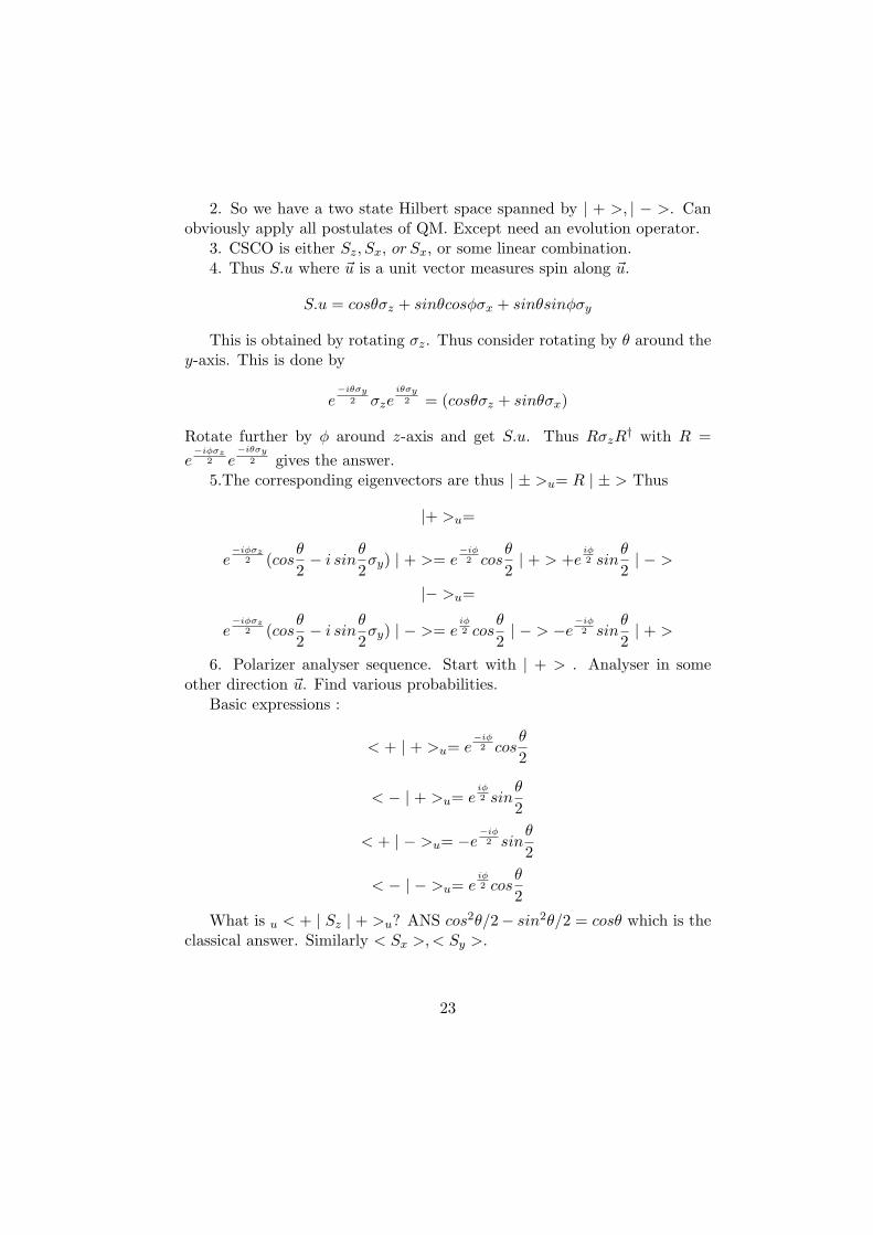
2. So we have a two state Hilbert space spanned by | + >, | − >. Canobviously apply all postulates of QM. Except need an evolution operator.

3. CSCO is either Sz, Sx, or Sx, or some linear combination.4. Thus S.u where ~u is a unit vector measures spin along ~u.

S.u = cosθσz + sinθcosφσx + sinθsinφσy

This is obtained by rotating σz. Thus consider rotating by θ around they-axis. This is done by

e−iθσy

2 σzeiθσy

2 = (cosθσz + sinθσx)

Rotate further by φ around z-axis and get S.u. Thus RσzR† with R =e−iφσz

2 e−iθσy

2 gives the answer.5.The corresponding eigenvectors are thus | ± >u= R | ± > Thus

|+ >u=

e−iφσz

2 (cosθ

2− i sinθ

2σy) | + >= e

−iφ2 cos

θ

2| + > +e

iφ2 sin

θ

2| − >

|− >u=

e−iφσz

2 (cosθ

2− i sinθ

2σy) | − >= e

iφ2 cos

θ

2| − > −e

−iφ2 sin

θ

2| + >

6. Polarizer analyser sequence. Start with | + > . Analyser in someother direction ~u. Find various probabilities.

Basic expressions :

< + | + >u= e−iφ2 cos

θ

2

< − | + >u= eiφ2 sin

θ

2

< + | − >u= −e−iφ2 sin

θ

2

< − | − >u= eiφ2 cos

θ

2What is u < + | Sz | + >u? ANS cos2θ/2− sin2θ/2 = cosθ which is the

classical answer. Similarly < Sx >,< Sy >.

23

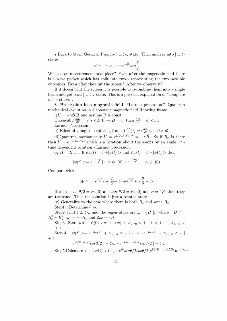
7.Back to Stern Gerlach. Prepare | ± >u state. Then analyze into | ± >states.

< + | − >u= −e−iφ2 sin

θ

2When does measurement take place? Even after the magenetic field thereis a wave packet which has split into two - representing the two possibleoutcomes. Even after they hit the screen? After we observe it?

If it doesn’t hit the screen it is possible to recombine them into a singlebeam and get back | ± >u state. This is a physical explanation of “completeset of states”.

8. Precession in a magnetic field. “Larmor precession.” Quantummechanical evolution in a constant magnetic field Rotating frame.

i)H = −γS.B and assume B is const.Classically d~m

dt = γ ~m×B If −γ ~B = ~ω, then d~mdt = ~ω × ~m.

Larmor Precession.ii) Effect of going to a rotating frame (d~mdt )X = (d~mdt )x − ~ω × ~m

iii)Quantum mechanically U = ei/2γ~B.~σt ~ω = −γ ~B. So if Bx is there

then U = e−i/2ωxσxt which is a rotation about the x-axis by an angle ωt -time dependent rotation - Larmor precession.

eg H = Hzσz. If ψ+(t) =< +|ψ(t) > and ψ−(t) =< −|ψ(t) > then

|ψ(t) >= e−iHzt

h |+ > ψ+(0) + e+iHzt

h |− > ψ−(0)

Compare with

|+ >u= e−iφ2 cos

θ

2|+ > +e

+iφ2 sin

θ

2|− >

If we set cos θ/2 = ψ+(0) and sin θ/2 = ψ−(0) and φ = Hzth then they

are the same. Thus the solution is just a rotated state.iv) Generalize to the case where there is both Bz and some Bx.Step1 : Determine θ, φ.Step2 Find | ± >u and the eigenvalues are ± | γB |. where | B |2=

B2x +B2

z . ω1 = −γBx and ∆ω = γBzStep3. Start with | ψ(0) >=| + >=| + >u .u < + | + > + | − >u .u <

− | + >Step 4. | ψ(t) >= e−iω+t | + >u .u < + | + > +e−iω−t | − >u .u < − |

+ >= eiφ/2−iω+tcosθ/2 | + >u −e−iφ/2−iω−tsinθ/2 | − >u

Step5:Calculate< − | ψ(t) > to get eiφsinθ/2cosθ/2(ei∆Ωt−e−i∆Ωt)e−iωavgt

24

Prob (t)= sin2θsin2∆Ωt where (∆Ω)2 = (∆ω)2 + ω21 and tan θ = ω1

∆ω9. Rotating magnetic field. Classical picture of resonance. Quantum

picture. NMR. d~mdt = γ ~m× (Bz ez +B1coswtex +B1sinwtey)

Go to rotating frame where B1(t) is time independent.(d~mdt )X = (d~mdt )x − ~ω × ~mIf γBz = −ω0 then we get(d~mdt )X = ~m× (w − w0)ez − ~m× w1eX.qm: Time dependent Hamiltonian!.

H = h/2

(ω0 ω1e

−iωt

ω1e+iωt ω0

)(15)

Going to rotating frame qm is done by | ψ >= e−iwt/2σzχ > is a definitionof χ > where Hamiltonian becomes time independent.

Equation becomes (Use e−iwtσz/2σxe+i.. = coswtσx + isinwtσy

ih ∂∂te

−iwt/2σz | χ >= e−iwt/2σz h/2(ω0σz + ω1σx) | χ >

⇒ ih ∂∂t | χ >= h/2[(ω0 − ω)σz + ω1σx] | χ >

P+−(t) =w2

1

w21 + (∆w)2

sin2(√w2

1 + ∆w2)t/2

When ∆ω = 0, the probability becomes 1 at some time. This is whenresonance occurs. So ω0 = ω. ω is the energy of the photon correspondingto oscillating field. ω0 is the energy difference. So hω = ∆E.

10. Other 2-level systems....(K0 − K0system). “Regeneration”. Gen-eral two level sytem and Spin 1/2 analogy.

25

4 Rotation Group

4.1 Symmetries and Conservation Laws

1. Physical idea of symmetry - translation, rotation, Lorentz transformation.Connection to coordinate transformation - the idea of manifest invariance ofequations/Hamiltonian/Lagrangian. Distinction between active and passivetransformation - one involves a physical movement whereas the other isa change of coordinates. But ultimately they amount to the same thingbecause “if the coordinate change leaves H invariant “you can’t tell fromwithin the system that you have moved”.

If H is invariant under translations, then [P,H] = 0. But this also meansP is constant in time. Conservation of momentum.

2. Transformation of other quantities: eg. background fields. If B 6= 0then rotation is not a symmetry, unless you rotate B also.

3. Practical application:i) when you choose a convenient coordinate sys-tem.

ii)Intuitive idea that the final result cannot contain such and such term:e.g by rotation/reflection symmetry the energy of a magnetic field cannotcontain Bx. It must be B2.

These ideas are made precise by group theory.4. Groups: mathematical objects that describe symmetry operations.

Multiplication, inverse, identity, closure. Discrete vs continuous. (Note:gh 6= hg in general - non commutative, but associative)

5. Discrete vs continuous groups. Lie groups. Lie algebras (additionis also included). Illustrate with translations. Dx(a) = eiaPx The idea ofexponentiation.

Generator = PxSimilarly Dy(b). Px, Py form an algebra. Dx, Dy form a group. Commu-

tation relation for algebra. Commutative (Abelian) vs Non abelian groups.

Dx(a)Dx(b) = Dx(a+ b) = Dx(b)Dx(a)

....Dx(a)Dy(b) = Dy(b)Dx(a)

Equivalent to[Px, Py] = 0

Explain the action on coordinates, wave functions, etc.Dx(a) : x→ x+ a and Dx(a)xD−1

x = x+ a (prove to second order)

26

[Px, x] = −iHere x is being treated as an operator.[iPx, x] = ∂xx = 1 is a particular representation of the operators in

x-space. Then Dx(a) = ea∂x

Acting on functions Dx(a)ψ(x) = ψ(x+ a).Rotations:

x′ = xcosθ + ysinθ

y′ = −xsinθ + ycosθ

Can write as a matrix. R(θ) = .... Also abelian - any one generator groupis abelian by defn.

6. Implications for qm: [G,H] = 0 G is the generator of a transfor-mation. Degeneracy. R(orG) | 1 >=| 2 > | 1 >, | 2 > have same energy.R | 2 >=| 3 > ... It will probably end somewhere if the group is compact.This defines an irrep. Dimension of the irrep is known from group theory.eg for rotation group. eg of spin 1/2. 2j + 1.

How does one define transf of wave fns.

ψ′(r′) = ψ(r)

Why? Defines a scalar. If r′ = Rr Then

ψ′(r′) = ψ(R−1r′)

⇒ ψ′(r) = Rψ(r) = ψ(R−1r)

eg Translations:

ψ′(x) = Rψ(x) = ψ(x− a) = e−a∂xψ(x)

where R is the effect of a translation by +a on the state. This gives

R = Dx(−a) = e−a∂x = e−iaPx

Note the signs.Action on kets:

| ψ′ >= R | ψ >

⇒< r | ψ′ >=< r | R | ψ >=< R−1r | ψ >

ThusR† | r >=| R−1r >

27

Clearly R†R = RR† = I So R is unitary. It is obviously linear. Soon states it is represented by a unitary matrix and the generators by aHermitian matrix.

Action on operators A′ = RAR†.7. Let us use this to find R for rotations: eg

ψ′(r) = Rψ(r) = ψ(R−1r) = ψ(x+ydφ, y−xdφ) = [1−dφ(x∂y−y∂x)]ψ(x, y)

Letx∂y − y∂x =

i

hLz

ThusR = 1− dφ i

hLz

This can be defined as the action of (infinitesimal) rotation about z on states.For finite rotaions Rz(φ) = e

−iφLzh . Physically: Rotates your system by +φ.

So if Hamiltonian is rotationally invariant about Z- axis [Lz,H] = 0.What is Lz? It is angular momentum. Check : Classically L = r X P . SoLz = xPy − yPx = −ih(x∂y − y∂x)

Similarlyi

hLx = y∂z − z∂y

i

hLy = z∂x − x∂z

Commutation relations

[Li, Lj ] = ihεijkLk

8. Implications for matrix elements. eg for integration : even and oddfns. The analog of this for more complicated groups. eg

∫einθdθ Using

invariance of measure dθ under θ → θ + a show that integral must bezero. So only singlets can be integrated to get non zero answer.∫ 2π

0dθf(θ) =

∫ 2π

0dθ′f(θ′)

Choose θ′ = θ + a. Consider In =∫ 2π0 dθeinθ. By change of variables

In =∫ 2π0 dθ′einθ

′=∫ 2π0 dθein(θ+a) = einaIn. We have used dθ = dθ′. ⇒

In[1− eina] = 0. So either n = 0 or In = 0.Get result that the integral is zero unless f is a singlet.

28

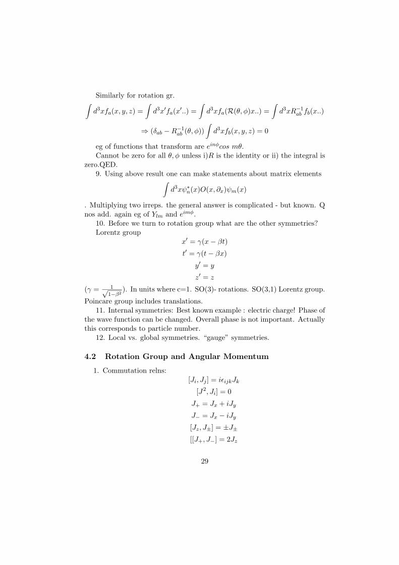
Similarly for rotation gr.∫d3xfa(x, y, z) =

∫d3x′fa(x′..) =

∫d3xfa(R(θ, φ)x..) =

∫d3xR−1

ab fb(x..)

⇒ (δab −R−1ab (θ, φ))

∫d3xfb(x, y, z) = 0

eg of functions that transform are einφcos mθ.Cannot be zero for all θ, φ unless i)R is the identity or ii) the integral is

zero.QED.9. Using above result one can make statements about matrix elements∫

d3xψ∗n(x)O(x, ∂x)ψm(x)

. Multiplying two irreps. the general answer is complicated - but known. Qnos add. again eg of Ylm and eimφ.

10. Before we turn to rotation group what are the other symmetries?Lorentz group

x′ = γ(x− βt)t′ = γ(t− βx)

y′ = y

z′ = z

(γ = 1√1−β2

). In units where c=1. SO(3)- rotations. SO(3,1) Lorentz group.

Poincare group includes translations.11. Internal symmetries: Best known example : electric charge! Phase of

the wave function can be changed. Overall phase is not important. Actuallythis corresponds to particle number.

12. Local vs. global symmetries. “gauge” symmetries.

4.2 Rotation Group and Angular Momentum

1. Commutation relns:[Ji, Jj ] = iεijkJk

[J2, Ji] = 0

J+ = Jx + iJy

J− = Jx − iJy[Jz, J±] = ±J±[[J+, J−] = 2Jz

29

2. CSCO

3. How nonlinearity fixes normalization. Thus σi do not satisfy the com-mutation relns: σi

2 do. Unlike Abelian case.

4. J± are raising lowering operators.

J+ | m >= const | m+ 1 >.

5. Show that |j,m > and |j,m±1 > are orthogonal using Jz, J+ commu-tation. Thus the states generated by rotations span a vector space ofsome dimensionality that can be worked out. This is the represen-taion. Explain the concept of a representation.

Fix const by using | J− | j,m >|2=< j,m | J+J− | j,m >

= j(j + 1)−m2 +m = (j +m)(j −m+ 1)

Eigenvalue of J2 being j(j + 1) is a convention. j is a real number.

| J+ | j,m >|2=< j,m | J−J+ | j,m >

= j(j + 1)−m2 −m = (j −m)(j +m+ 1)

SoJ+|j,m >=

√j(j + 1)−m(m+ 1)|j,m+ 1 >

.

6. Show

:i) −j ≤ m ≤ j

ii) J− | j,−j >= 0 but J−|j,−j + ε >6= 0.

J+ | j, j >= 0 but J+|j,m− ε >6= 0.

iii) The value of m closest to −j, if it is a little larger than −j (canalways be made to lie between −j,−j + 1) we get a contradiction.Because on the one hand J− acting on that has to give zero, becausem − 1 < −j. On the other hand the norm of J−|j,m > is not zero ifm > −j. Only possibility is that the m must be precisely = −j.Thus the difference between −j and m must be an integer. Similarlybetween j and m. Thus we have :m− p = −j and m+ q = j.

Therefore j = (q + p)/2.⇒ j is integer or half integer

30

7. Matrix elements :

< j,m | Jz | j′,m′ >= δj,j′δm,m′m

< j,m | J± | j′,m′ >= δj,j′δm,m′±1

√j(j + 1)−m(m± 1)

As an example of the group theoretic selection rule.

8. Examples of representations: j=0,1/2,1. What they act on.

4.3 Orbital Angular Momentum and Ylm1.

Lx =h

i(y∂z − z∂y)

etc. Physical idea of orbital vs spin.

Write this in terms of θ, ∂θ, φ, ∂φ

2. Change of variables:x, y, z → r, θ, φ. Volume element d3x = r2drdΩ =r2drdφd(cosθ)

Ylm =< θ, φ | l,m >

This is the definition. Like

< x | k >= eikx

3. Just as eikx is a soln of ∂xψ(x) = kψ(x) we need eqns for Ylm.

L+Yll = 0

LzYlm = mYlm

4. Need Lj expressions in spherical coordinates.

Lx = i(sinφ∂θ +cosφ

tanθ∂φ)

Ly = i(−cosφ∂θ +sinφ

tanθ∂φ)

31

Lz = −i∂φL+ = eiφ(∂θ + icotθ∂φ)

L− = e−iφ(−∂θ + icotθ∂φ)

L2 = −(∂2θ +

1tanθ

∂θ +1

sin2θ∂2φ)

Need ∂φ∂y etc. Work out one say Lx.

y∂

∂z= y

∂

∂φ

∂φ

∂z+

∂

∂θ

∂θ

∂z

z = rcos θ

ρ = rsin θ =√x2 + y2

Suppose we change z to z + dz. Clearly φ doesn’t change. So firstterm is zero.

tan (θ + dθ) = tan θ + sec2 θdθ

=ρ

z + dz=ρ

z− ρdz

z2= tan θ − sin θ

rcos2 θdz

Sodθ

dz= −1

rsin θ

z∂

∂y= z

∂

∂φ

∂φ

∂y+

∂

∂θ

∂θ

∂y

Change y to y + dy.

tan (θ + dθ) = tan θ + sec2 θdθ =ρ+ dρ

z

=ρ

z+ydy

ρz= tan θ +

sin θdy

rcos θ

∂θ

∂y= cos θsin φ

32

Thus toatl coefficient of ∂∂θ is −sin φ.

Coefficient of ∂∂φ :

y + dy

ρ+ dρ= sin(φ+ dφ)

y

ρ+dy

ρ− ydρ

ρ2= sin φ+

x2dy

ρ3

⇒ cos φdφ =cos2 φ

rsin θdy

So z∂y = cosφtanθ∂φ

Add everything to get Lx. etc.... ..

.

5. Using Lz get Ylm(θ, φ) = Flm(θ)eimφ

andL+Yll = 0 ⇒ [−∂θ + cotθl]Fll = 0

dF =ld(sinθ)sinθ

F

F = c(sinθ)l

Yll = ceilφsinlθ

Get the rest by using lowering operators.

Example:Y11(θ, φ) = c eiφsin θ

where c is a normalization constant.

L−Y11 = e−iφ(∂θ + icot θ∂φ)(ceiφsin θ)

⇒√

2Y10 = −2c cos θ

Y10 = c√

2cos θ

L−Y10 =√

2Y1−1 =√

2 c e−iφsin θ

⇒ Y1−1 = c e−iφsin θ

33

6. Orthogonality: ∫dΩY ∗lm(θ, φ)Ylm(θ′, φ, ) = δll′δm,m′

Closure:∞∑l=0

Ylm(θ, φ)Y ∗lm(θ′, φ′) = δ(cosθ − cosθ′)δ(φ− φ′)

The delta fns satisfy∫dΩδ2 = 1

7. Explicit expressions:

Y1,±1(θ, φ) =√

38πsinθe±iφ

Y1,0 =√

34πcosθ

Cartesian representation x,y,z !!!

Similarly Y2,m(θ, φ) are essentially xixj these five.

Check that they satisfy Rψ(r) = ψ(R−1r)

8. Observables transform as A′ = RAR†

[V, Ji] = 0 ⇒ V is a scalar

[Vi, Jj ] = iεijkVk ⇒ V is a vector.

J itself is therefore a vector.

9. Spin vs Orbital ang momentum. eg. If ψ itself happens to be avector, ψ′(Rr) = Rψ(r). Thus ψ′(r) = Rψ(R−1r). The R outsideis implemented by ~dφ × ~ψ. Which is −i ~dφ.~S where S is i times thematrix that implements the cross product. eg

Sz = i

0 −1 01 0 00 0 0

(16)

implements rotaion about z-axis. (−i.i = 1). The R−1 inside is im-plemented as already seen by −i ~dφ.~L. So total generator is S + L. Sis spin.

34

10. Addition of Angular Momentum - Clebsch Gordan coeff.

The product of two representations must be a representation - in thesense that the generators will not take you out of that set. But it maybe reducible. Thus:

∑j

c(j) | j,m(= m1 +m2) >=| j1,m1 > ⊗ | j2,m2 >

The max value on RHS is m1 = j1 and m2 = j2. So max on LHS ismmax = j1 + j2. This must be the max value of m of some jmax Thusjmax = j1 + j2. No other (smaller) value of j can give this m. Thuswe have

|j1 + j2, j1 + j2 >= |j1, j1 > ⊗|j2, j2 >

Use J± | j,m >=√j(j + 1)−m(m± 1) | j,m± 1 > Get

| j1+j2, j1+j2−1 >=

√j1

j1 + j2| j1−1 > ⊗ | j2 > +

√j2

j1 + j2| ji > ⊗ | j2−1 >

The orthogonal state is

| j1+j2−1, j1+j2−1 >=

√j2

j1 + j2| j1−1 > ⊗ | j2 > −

√j1

j1 + j2| ji > ⊗ | j2−1 >

Example: spin 1/2| 1, 1 >=| ++ >

| 1, 0 >=√

12[| +− > + | −+ >]

| 1,−1 >=| −− >

The orthogonal combination:

| 0, 0 >=√

12[| +− > − | −+ >]

The above was an example of calculation of Clebsch-Gordan coeffi-cients.

35

11. Clebsch-Gordan:

| J,M >=∑

m1,m2

| j1,m1; j2,m2 > < j1,m1; j2,m2 | J,M >︸ ︷︷ ︸Clebsch−Gordan

| j1 − j2 |≤ J ≤ j1 + j2

Recursion reln for C-G:

Act with J− on LHS and J1− + J2− on RHS and apply< m′1,m

′2 | to

get

√J(J + 1)−M(M − 1) < m′

1,m′2 | J,M − 1 >

=√j1(j1 + 1)−m′

1(m′1 + 1) < m′

1 + 1,m′2 | J,M >

+√j2(j2 + 1)−m′

2(m′2 + 1) < m′

1,m′2 + 1 | J,M >

Another reln where +1 and -1 are interchanged. General procedure:

As in the example above we started with |j1 + j2, j1 + j2 > and got|j1 + j2, j1 + j2 − 1 >. Then by orthogonality we got |j1 + j2 − 1, j1 +j2 − 1 >.

Continue: Use these relations to get |j1 + j2, j1 + j2 − 2 >, |j1 + j2 −1, j1 + j2 − 2 >. Then by orthogonality get |j1 + j2 − 2, j1 + j2 − 2 >.Keep going and work out all the C-G’s.

12. Wigner-Eckart:

i). Scalar operator A: Using [J2, A] = 0 = [Ji, A] we can show that

< j′,m′ | A | j,m >= δjj′δmm′a(j)

From

< j′,m′|[J2, A]|j,m > = 0 = < j′,m′|[Jz, A]|j,m >

we see that j = j′ and m = m′.

To see that the matrix element doesn’t depend on m:

< j,m|J−AJ+|j,m >= [j(j + 1)−m(m+ 1)] < j,m+ 1|A|j,m+ 1 >

36

Also:

< j,m|J−AJ+|j,m >=< j,m|AJ−J+|j,m >= [j(j+1)−m(m+1)] < j,m|A|j,m >

Thus the matrix elements do not depend on m. So any two scalarsmatrix elements are proportional in the entire (j,m) subspace.

ii) For vectors ~V : Can show that:

< j,m′ | ~V | j,m >= a(j) < j,m′ | ~J | j,m >

i.e. the prop const is ind of m:

Use [V+, J+] = 0 and the fact that V+ has m = 1. Thus

< j,m+ 2|V+J+|j,m >=< j,m+ 2|J+V+|j,m >

Insert complete set of states: Only |j,m+ 1 > contribute. so

< j,m+2|V+|j,m+1 >< j,m+1|J+|j,m >=< j,m+2|J+|j,m+1 >< j,m+1|V+|j,m >

Thus

< j,m+ 2|V+|j,m+ 1 >< j,m+ 2|J+|j,m+ 1 >

=< j,m+ 1|V+|j,m >

< j,m+ 1|J+|j,m >= C+(j)

Similarly with V− we get C−.

Finally, using [V+, J−] = 2Vz we find on inserting a complete set ofstates, < j,m|Vz|j,m >= C+m. If we use [V−, J+] = −2Vz we get< j,m|Vz|j,m >= C−m. Thus C+ = C−.

Thus if P is proj operator into j-subspace:

PJ.V P = a(j)PJ.JP = a(j)j(j + 1)P

⇒ a(j) =J.V

j(j + 1)

in the given subspace.

Useful: iii) spinning electron in a magnetic field: H1 = wl(Lz + 2Sz).

J = L+ S

CSCO:Jz, J2, L2, S2

37

Thus if we neglect mixing between different valus of j for small B-field.

< J,M, S, L | H1 | J,M, S, L >= wl< J.L > +2 < S.L >

J(J + 1)Jz

= (3/2 +S(S + 1)− L(L+ 1)

2J(J + 1))Mwl

“Lande’s g-factor” - splits the degeneracy.

iv) General Wigner-Eckart: matrix elements of TQ,K are proportionalto clebsch-Gordan:

< j,m | TQ,K | j′,m′ >= a(j, j′)< j,m | Q,K; j′m′ >︸ ︷︷ ︸C−G

Use CG to write

TQ,K | j′,m′ >=∑J

NJ | J,M >< J,M | Q,K; j′,m′ >

TQ,K | j′,m′ >=∑J

| J,M >< J,M | TQK | j′,m′ >

These two equations are proportional in each J, j′, Q sector. Becauserotaion of coordinate systems will change M,K,m′ in exactly the sameway in both equations. So the proportionality constant NJ cannotdepend on M .

As a special case consider

TQQ|j′, j′ >= a(Q+ j′, j′)|Q+ j′, Q+ j′ >

Let

TQ,Q−1|j′, j′ >=

√Q

Q+ j′a1|Q+j′, Q+j′−1 > −

√j′

Q+ j′b1|Q+j′−1, Q+j′−1 >

Take the matrix element:

< Q+ j′, Q+ j′ − 1|TQQ−1|j′, j′ >=

√Q

Q+ j′a1

38

LHS can be written as

1√2(Q+ j′)

< Q+j′, Q+j′|J+TQQ−1|j′, j′ >=1√

2(Q+ j′)< Q+j′, Q+j′|[J+, TQQ−1]|j′, j′ >

=

√Q

Q+ j′< Q+ j′, Q+ j′|TQQ|j′, j′ >=

√Q

Q+ j′a(Q+ j′, j′)

a1 = a(Q+ j′, j′)

Similarly for the rest, by recursion. The above calculation implementsthe idea od rotating the coordinate system.

More general proof (a la Schiff): Want to show that TKQ|j,m >=∑J |J,M >>< J,M |Q,m >. Here< J,M |Q,m > are the C-G’s. The

sum is over all allowed values of J. |J,M >> transforms like an angularmomentum state, but its normalization depends on T . Want to showthat this normalization cannot depend on M . So invert the above:

|J,M >>=∑Q,m

TKQ|jm >< Q,m|J,M >

Act with J+.

RHS gives:∑Q,m

√K(K + 1)−Q(Q+ 1)TKQ+1|j,m >< Q,m|J,M >

+√j(j + 1)−m(m+ 1)TKQ|j,m+ 1 >< Q,m|J,M >

Let Q′ = Q+ 1 in the first term and m′ = m+ 1 in the second term.

=∑Q′,m

√K(K + 1)−Q′(Q′ − 1)TKQ′ |j,m >< Q′ − 1,m|J,M >

+∑Q,m′

√j(j + 1)−m′(m′ − 1)TKQ|j,m >< Q,m′ − 1|J,M >

Note that the range of Q′,m′ is the same as Q,m because the extraterm vanishes anyway. Drop the primes.

39

If you use the recursion relation RHS becomes√J(J + 1)−M(M + 1)

∑Q,m

TKQ|j,m >< Q,m|J,M + 1 >

=√J(J + 1)−M(M + 1)|J,M + 1 >>

.

The last equality implies that the proprtionality between |J,M > andJ,M >> is the same for all M . In particular if we know one <j′,m′|TKQ|j,m > we know all the rest (i.e. other values of m,m′, Qand same j, j′,K) by using C-G relations. This is the Wigner EckartTheorem.

4.4 P,T,C

Motivate by asking the question “ How does one communicate the conceptof left-handed to a Martian?” This is the idea of symmetry. Ans. W−

decay. It decays into left handed electrons!Parity:1.

P~r = −~r

On the ket:P |r >= | − r > .

i)As a matrix P has det =-1. Not a rotataionii)Mirror Reflection (z → −z) followed bey rotation about z-axis by 180

gives parity.2.

ψ′(r′) = wψ(r)

Allowed as parity is discrete.

Pψ(r) = wψ(−r)

However for integer spin can require that P 2 = 1 So w2 = 1 and w = ±1.Thus for the operator r

3. PrP−1 = −r , PpP−1 = −p but PLP−1 = L same for S and J .In polar coordinates θ → π−θ and φ→ φ+π. Ylm → (−1)lYl,m. Check.Current: ~j → −~j and ρ→ ρ.

40

So φ(x) → φ(−x), ~A → − ~A Thus photon has intrinsic parity -1. E →−E B → B (Axial vectors)

4. If parity is conserved PHP−1 = H. This implies PSP−1 = S.eg π0 → 2γ. What is the intrinsic parity of π0 Does it have defn parity?

If yes : J=0 means the final state wave fn must be a scalar depending on~ε1,~ε2, k.

~ε1.~ε2

or(~ε1 × ~ε2).k

It is found that π0 has P=-1 - pseudoscalar.In terms of helicities ψRR ± ψLL are the two photon states with defn

parity.5. Parity is violated.eg when a W decays (e−, ν) the electron coming out

is always left helicity.Charge ConjugationSupoose the Martian doesn’t know what is +ve and -ve charge. Then

how would he distinguish between theW− decaying into left handed electronand W+ decaying into right handed positrons? He can’t!

1.e− → e+

CH = HC and so CS = SC. Unitary.2.

φ→ −φ~A→ − ~A

⇒ photon has intrinsic C of -1. Does nothing to r, t.examples: 3. π0 → 2γ 2 photons state has C =+1. So the pion has

C=+1. Which means π → 3γ is not allowed!4.Furry’s theorem: No. of external photons must be even. (−1)n =

(−1)m ⇒ n+m is even.5. Positronium: e+e−. The electron has r, S, C quantum nos and we

interchange electron and positron. Fermions , so overall sign has to benegative.

(−1)l(−1)s+1C = −1

So C = (−1)l+s. Thus1S0 → 2γ

(spin =0, l=0)3S1 → 3γ

41

(spin 1, l=0) but not 2γ.6.CPK0 = sd and K0 = sd.

K0 − K0

√2

has C=-1 and P=-1 so CP=1

K0 + K0

√2

has C=1 and P=-1 so CP=-12π0 has P=1 (S-wave), C=1 So CP=1. 3π0 has P=-1 (S-wave) and C=1

so CP=-1. (It has to be S-wave because the K’s are J=0)The K-Kbar goes into 2π and is faster decay - henceKS and the other one

is called KL CP odd and longer lived. These are also the mass eigenstates.But in fact occasionally KL decays into 2π: violates CP.So in fact there may be a difference between W+ decay and W− decay!

So the Martian will be able to distinguish between left and right after all!.Unless he doesn’t know the difference between time going forwards and

backwards!Time Reversal:1. Tψ(x, t) = cψ(x,−t) Schroedinger eqn doesn’t have this symmetry!

Because it is first order. Assume T is unitary. If we take a state at t=0 andpropagate to t and then time reverse, or time reverse and then propgate to-t, we should get the same answer.

Te−iEtu = e−iEtTu

other wayeiEtTu

. Want anti linear: T (aψ(x, t)) = a∗T (ψ(x,−t))This will solve the problem. So

T = UK

where U is unitary and K is antilinear - “complex conjugation” - i.e Kψ =ψ∗.

< φ | ψ >=< ψ | φ >∗=< Tψ | Tφ >

But in general U,K will depend on the representation.

42

2.rT = Tr

pT = −Tp

TL = −LT

TYlm = Y ∗lm

(T does nothing to θ, φ)

ρ→ ρ

j → −j

φ→ φ

A(x, t) → −A(x,−t)

E → E

B → −B

3. Spin is like L. Want to reverse. σy is imaginary so K does the job.σx , σz need to be reversed: e−iπSy will do that. So

T = e−iπSyK

. This argument works for any spin. Sy can always be chosen imaginary.For spin 1/2 T = −iσyK.T 2 = e−i2πSy which is +1 on integer spin and -1 on half integer.4. Application Kramer’s degeneracy. Can electric field lift degeneracy?Suppose there is no degeneracy due to T. Then Tuk = cuk must be true

for c a number. T 2uk =| c |2 uk. Now if we are talking of a half integer then| c |2= −1 is a contradiction. So there must be a degeneracy! Regardlesshow complicated the electric field.

B breaks the symmetry.TYlm = cYlm is possible only for m=0 or for states like Ylm±Yl−m. Thus

m is not a good quantum no.

43

5 Harmonic Oscillator

5.1 Review

1. Importance of harmonic oscillator: Leading Aproximation.

2. Hamiltonian and Lagrandgian.

H =P 2

2m+mω2

2X2

Rescaling variables.

Let X ′ =√mX and P ′ = P√

m. [X ′, P ′] = ih.

H =12(P ′2 + ω2X ′2)

Rescale again: X = 1√ωX ′ and P =

√ωP ′.

H =ω

2(P 2 + X2)

Thus x =√ωx′ =

√mωx. Drop hats from now on.

Creation operator a† = (X − iP )/√

2h and [a, a†] = i.

3. Eigenstates: | n > : a† | n >=√n+ 1 | n + 1 > Number operator

N = a†a , H = hω(N + 1/2).

4. Wave fns.(x+

∂

∂x)ψ = 0 ⇒ d(ln ψ) = −1

2d(x2)

ψ(x) ≈ e−x2

2 ≈ e−mωx2

2

We have rescaled from hat variables to ordinary variables.

φ0 = (mωπh )1/4e−mωx2

2h X Hermite polynomials.

44

5.2 Path Integral Treatment

1. Doing Gauusian integrals:∫ x(tf )=xf

x(ti)=xiDx(t)︸ ︷︷ ︸

sumover paths

exp(+ ih

∫ tfti dtL(x(t), ˙x(t))

with L = T − V (x) where V is quadratic.Let x(t) = xc(t) + y(t). Then Xc satisfies bc. So y is 0 at both ends. So

we get∫ x(tf )=xf

x(ti)=xiDx(t)︸ ︷︷ ︸

sumover paths

exp(+ ih

∫ tfti dtL(x(t), ˙x(t)) = F (ta, tb)e

ihScl

whereF (ta, tb) =

∫y(ta)=y(tb)=0

Dy(t)ei∫ tb

tadtL(y,y,t)

and of course L is quadratic.Time independent implies F (ta − tb)2. Do the calc for SHO. First Sc, then F. Done before.3. Evaluate φ0(x) and φ1(x) by expanding kernel.

2 coswt = eiwt(1 + e−2iwt)

2i sinwt = eiwt(1− e−2iwt)

5.3 1-dim crystal and field theory

1. Want to solve:

L =N∑j=1

1/2q2j − ν2/2(qj+1 − qj)2

2. Special case of coupled oscillators:

L =12[(q21 + q22) + q21 + q22 + αq1q2]

If we define Q = q1+q2√2

and q = q1−q2√2

, then

45

L =12[(Q2 + (1 + α)Q2 + q2 + (1− α)q2].

Gives a decoupled system.

Can get q1(t) = Q(t)+q(t)√2

and q2(t) = Q(t)−q(t)√2

.

If α = −1, then we have diatomic molecule - centre of mass is free.The crystal is a generalization of this.

Now general case:

3. Periodic bc qN+1 = q0.

4. Eqn of motion.

d2qndt2

= ν2(qn+1 − qn) + (qn−1 − qn)

Solns. Use translation inv. to get the normal modes.

qn = eiβn

are the form of normal modes with β = 2πkN

eiβn−ωt = eiβa(x−aνt)

vel is

c = aν

w2 = ν2(4sin2β

2)

5. Show that normal modes are decoupled oscillators.

qn =1√N

∑k

akeiβkn

L = 1/2∑k

[aka−k − 4ν2sin2βk/2aka−k]

Also need to divide by√N to get finite limit.

46

Reality of qn(t) implies a∗k(t) = a−k(t) But a−k = aN−k. So a∗k =aN−k. Define

bk = 1/2(ak + a∗k) = 1/2(ak + aN−k)

andck = 1/2i(ak − aN−k)

The index on b,c clearly go only to N/2. In terms of b,c:

L = 1/2

N2∑

k=1

[(bk)2 − 4ν2sin2βk2b2k] + same for c

With time dep

qn(t) = akeiβkn−iwkt + a∗ke

−iβkn+iwkt

= bk cos(βkn− wkt)− ck sin(βkn− wkt)

What happened to waves in the opp direction: by changing βk →βk− 2π = βk−N we get waves moving the opposite way! So if we wantwe can change all the indices on the c to negative. Thus N − k ≡ −k.Whichever way you count there are N oscillators.

6. Continuum limit. “ Free Field Theory”. The velocity of light emerges.qn(t) → q(x, t).

L = 1/2∫dx[

q2

a− ν2a(q′)2]

1/2∫dx[Q2 − c2Q′2]

where q = Q√a

In terms of oscillators ∑k

b2k − 4ν2sin2(βk2

)b2k

In cont. limit 4ν2sin2... = (2πkνN )2 = w2

k. Thus we have harmonic oscwith energy quanta =

hw =h2πkνN

=h2πkL

c = pc

phonons / photons ...

47

5.4 Coherent States

1. Rescale √mwX = x

P√mw

= p

.

2. Classical eqns x = ωp and p = −ωx. Can be written as

α = −iωα

Want same eqns qm.for < a >

ihd/dt < a >=< [a,H] >= ω < a > (t)

3. Find a state such that < a >= α0 and also < H >= hω | α0 |2 =classical.

Leta | α >= α | α >

This will solve the problem.

| α >= e−|α|2/2∑n

αn√n| φn >

4. Props: i) closure

1π

∫dRe αd Im α|α >< α| =

∑n

|n >< n| = 1.

Note that the measure is dx dp2π .

ii) not ortho. They are over complete:

< α | α′ >= e−|α|2

2 e−|α′|2

2

∑n

(α∗)n√n

(α′)n√n

= e−|α|2

2 e−|α′|2

2 eα∗α′

Thus | < α|α′ > |2 = e−|α−α′|2 6= 0.

48

5.

< H >α= hw[| α |2 +1/2]

< H2 >α= hw[| α |4 +2 | α |2 +1/4]

∆H = αw∆HH

= 1/α ≈ 0

Same for X,P

< X >,< P >= Re, Im(α)√

2

< X2 > − < X >2= 1/2

Find∆X∆P = 1/2

Minimum uncertainty.

6. Unitary operator D(α) | 0 >=| α >D = eαa

†−α∗a. DD† = 1.

< x | α >=< x | D | 0 >

αa† − α∗a = (α− α∗)x/√

2− i(α+ α∗)P/√

2

Using eA+B = eAeBe−12[A,B],

D = eα∗2−α2

4 e(α−α∗)x√

2 e−i(α+α∗)p√

2

It follows that

ψ(x, 0) = eiθei<P>xφ0(x− < X >)

φ0 is the gnd statet wave fn. Width of gaussian is 1/√

2 for x or√

h2mw

for x.

7. Time dependences of everything. Coherent states remain coherent.

| α(t) >= e−iwt/2 | α(0)e−iwt >

Wave packet remains a wave packet. So at later times also we getsame wave fn except that < x > and < p > change with time as coswt , sin wt etc. and also we get an overall phase.

49

6 Perturbation Theory

6.1 Stationary Perturbation Theory

1.H = H0 + V

Matrix elements of V are assumed to be smaller than E0n−E0

p Let V = λWwhere λ is a small number and matrix elements of W are not small.

2.H(λ) | ψ(λ) >= E(λ) | ψ(λ) >

LetE(λ) = ε0 + λε1 + λ2ε2 + ...

| ψ(λ) >=| 0 > +λ | 1 > +λ2 | 2 > +...

We getH0 | 0 >= ε0 | 0 >

(H0 − ε0) | 1 > +(W − ε1) | 0 >= 0

(H0 − ε0) | 2 > +(W − ε1) | 1 > −ε2 | 0 >= 0

Assume < ψ | ψ >= 1 and phase convention < ψ | 0 > is real.⇒< 0 | 0 > +λ < 0 | 1 > is real. So < 0 | 1 > is real.Also < 0 | 0 > +λ < 0 | 1 > + < 1 | 0 >= 1. Plugging in lowest order

solution which is < 0 | 0 >= 1 and using reality get < 1 | 0 >= 0.Solution:Zeroeth order gives

| 0 >=| φn >

1st order Applying < φn |

ε1 =< φn |W | φn >

Applying < φp | gives

| 1 >=∑p,p6=n

< φp |W | φn >En − Ep

| φp >

2nd order Apply < φn| to second order equation:

ε2 =∑p,p6=n

< φn |W | φp >< φp |W | φn >En − Ep

50

Note sign: decided by En − Ep. eigen value repulsion.2. Degenerate Perturbation theoryLet | φin > : i = 1, .., gn be states degenerate in energy.first order eqn is modified: get a matrix eqn insted of a single eqn:

Apply< φin | to get

< φin |W | 0 >= ε1 < φin | 0 >

Insert complete set of states and use orthogonality to restrict sum to sub-space. ∑

j

< φin |W | φjn >︸ ︷︷ ︸gn×gn matrix

< φjn | 0 >= ε1 < φin | 0 >

This may or may not split degeneracy. But W has been diagonalized soneed not fear infinite denominators.

Degeneracy is important because it is qualitative and not quantitative.If due to symmetry, higher orders will not resolve it.

6.2 Applications

1.Anharmonic oscillator

H0 = 1/2hw(P 2 +X2)

V = λhwX3

Non zero matrix elements of pert:

< φn+3 | V | φn >=hw

2√

2

√(n+ 1)(n+ 2)(n+ 3)

< φn−3 | V | φn >=hw

2√

2

√n(n− 1)(n− 2)

< φn+1 | V | φn >=3hw2√

2

√(n+ 1)3

< φn−1 | V | φn >=3hw2√

2

√n3

ε1 =< φn | V | φn >= 0

51

2nd order

| < φn+3|V |φn > |2

−3hω= − hω

3(n+ 1)(n+ 2)(n+ 3)

8

| < φn−3|V |φn > |2

+3hω=hω

3n(n− 1)(n− 2)

8

| < φn+1|V |φn > |2

−hω= −9hω

(n+ 1)3

8

hw

−24(n+ 1)(n+ 2)(n+ 3) +

hw

24n(n− 1)(n− 2) + w9/8n4 − hw9/8(n+ 1)3

= −15/4(n+ 1/2)2hw − 15/2nhw

×λ2.Note En−En−1 = hw−15/2nλhw. The energy difference is not constant.Eigenstate is of the form

| ψn >=| φn > +O(λ)(| φn+3 >, | φn−3 >, | φn+1 >, | φn−1 >)

,2. Applications : Oscillating dipole normally radiates only Bohr frequen-

cies w. But the anharmonic X connects n with n+2 and also n-2.This is because < ψ2|X|ψ0 >≈ λ < φ1|X|φ0 > O(λ) 6= 0. So we get

frequencies corresponding to E2 − E0 ≈ 2ω. So we get 2w also.Even < ψn | X | ψn >6= 0, ≈ O(−λn3/2). This implies at higher n

the dipole stretches. When λ is negative it is easier to move to the right(+ve x) than to the left. Vice versa when λ is positive. So at higher energylevels expect that average x will change in the direction which is easier. Thisexplains the sign in the equation and also explains why materials expand onheating.

Van der Waal’s force

1. Potential due to a charge = φ(r) = qr . Potential due to a dipole

φ(r) =q

r− q

r + δr=qδr

r2=q~rD.r

r2=~p.r

r2=~p.~r

r3

52

Electric field due to dipole:

Ei = −∂iφ(r) = −(pi

r3+ ~p.~r

∂

∂i(

1r3

))

= −(pi

r3+ ~p.~r(

−3ri

r5))

Ei = −pj [δijr3− 3rirj

r5]

Energy − ~E1.~p2:

W = pi1pj2[δijr3− 3rirj

r5]

2. We are considering force between two neutral atoms, that have nodipole moments. Say, hydrogen atoms in their ground states. Thestate is |ψ0 >= |1 > ⊗|2 > orψ0(r1)ψ0(r2). We are given that <1|p1|1 >=< 2|p2|2 >= 0. Therefore < ψ|W |ψ >= 0.

No first order correction.

3. Second order: ∑n6=0 < ψn|W |ψ0 > |2

E0 − En

Note the sign: it is negative (E0 < En) : ⇒ attractive.

Since W ≈ 1r3

, the van der Waal correction is ≈ 1r6

. ∆E = − cr6

. Letus estimate c.

4. E0 = E10 + E2

0 . For each atom, |En| = |E0n2 | << |E0|. So we drop En.

Then

∆E =∑n

| < n|W |0 > |2

E0

=< 0|W 2|0 >

E0

Choose the direction between the atoms to be z. So we get

W ≈ p1xp2x + p1yp2y − 2p1zp2z

W 2 = e4(x1x2 + y1y2 − 2z1z2)2

53

We need < 0|W 2|0 > so all cross terms can be dropped.

< W >=< x1x1 >< x2x2 > + < y1y1 >< y2y2 > +4 < z1z1 >< z2z2 >

By symmetry they are all equal to < r2

3 >< r2

3 > . For the hydrogenatom < r2

3 >= a20. Also E0 = 2 e2

2a20

- the factor of 2 because there are

two atoms. Thus we get c = 6e2a50.

5. Physical mechanism: QMec fluctuation produces a dipole moment inone atom, which induces a dipole in the second atom and they attract.These two dipoles are correlated because one is induced by the other.The uncorrelated fluctuations average out.

Because one dipole induces the other there is a time lag. So when thetime taken for influence is of the order of Bohr frequency, this approxbreaks down. Thus r < c

ν = λ. Also R should be large enough thatthe independent wave function approx holds.So r >> a0.

6.3 Time dependent pert theory

We ask for transition prob from some initial state i to some final state fusually during the perturbation or after. Usually i and f are eigenstates ofunperturbed H. Special case 1) Adiabatic 2) Sudden.

Otherwise do pert in λ as before.

ihd/dt | ψ(t) >= (H0 + λV | ψ(t) >

ψ(0) >=| φi >

Reqd:Pfi(t) =|< φf | ψ(t) >|2

|ψ(t) >=∑k

ck(t)|φk >

ck(0) = δki Project < φn | to get

ihcn =< φn | H0 + λW |∑k

ck | φk >

Insert complete set of states:

=∑m

(Enδnm + λWnm)cm(t)

54

Redefine cn(t) = bn(t)e−iEnt to get

ihd/dtbn(t) = λ∑

Wnmeiwnmtbm

Now expandbn = b0n + λb1n + ..

Solnb0n = const = δni

b1n(t) =1ih

∫ t

0dtWnie

iwnitdt

Pfi(t) = 1/h2 |∫ t

0dtWnie

iwnitdt |2

special case i) harmonic perturbation W (t) = Wsinwt or Wcoswt. Ifω = 0 use cos to get:

|Wfi |2

h2 [sinwfit/2wfi/2

]2

If w 6= 0 use 2sin wt and get same formula with wfi → wfi − w.Coupling to continuum:Use (sinwt/2/w/2)2 = 2πthδ(Ef − Ei).Derivation: ∫ ∞

−∞eixtdt = 2πδ(x)

= limT→∞

∫ T

−Teixtdt =

2i sin xTix

⇒ LimT→∞sin xT

x= πδ(x)

LimT→∞(sin xT

x)2 = πδ(x)

sin xT

x= πTδ(x).

For the case ω = 0,

dPfi/unittime/dβ =2πh|< β,E |W | φi >|2 ρ(β,E = Ef = Ei)

Here β represents any other continuous parameter (eg. angle). ρ(β,E)is the no. of states per unit ∆E, per unit ∆β. (“number density of states”).This is Fermi Golden Rule

55

2. Prove Born scattering formula: Take initial state to be | pi > andfinal state to be | pf >. Note: < x|p >= eip.r This is different from that insome books where < x|p >= 1

(2πh)32eip.r.

Calculate ρ(E). ∫d3p

(2πh)3=∫dΩdEρ(E)

(In the other normalization there would be no factors of 2π.)∫p2dpdΩ(2πh)3

=∫

pm

(2πh)3dEdΩ =

∫ √2mEm

(2πh)3dEdΩ

Thus ρ(E) = m√

2mE(2πh)3

.Divide final probability/unit time by flux (= p

m)to get prob /unit flux/unittime.

m2

4π2h4 |∫d3rei(pf−pi).rW (r) |2

[If we use the other normalization we also get same. But ρ(E) = m√

2mE.The factors of 2π are in the matrix element.]

This is called the “differential scattering cross section”.The total scattering cross section will now involve integration over dΩ.

6.4 Scattering

1.

dn = σ(θ, φ) Fi dΩ

where Fi is the incident flux and σ(θ, φ) is the differential scatteringcross ection. It is no. of scattered particles per unit incident particleper unit solid angle. ∫

dΩσ(θ, φ) = σ

is total scattering cross section.

2. Calculation of σ.

Look for stationary states:

[− h2

2m4+ V (r)]φ(~r) = Eφ

56

Let 2mV/h2 = U and let h2k2 = 2mE, then

[4+ k2]φ(~r) = U(r)φ(~r)

Now the soln we want has the asymptotic form

φ(r) ≈ eikz + f(θ, φ)eikr/r

Because it has the form of incident wave plus outgoing scattered wave.and eikr/r is also a soln to the homogeneous eqn as long as r > 0. Tosee that:

4(1/r) = 4πδ(~r)

- from electrostatics. Note that this is the three-dimensional deltafunction. Can check that − e±ikr

4πr = G±(r) is the Green fn [Do theyknow what it is?] for Scattering eqn above. [Use 4 = ∂2

∂r2+ 2∂

r∂r ]

The incident flux is hkm and scattered flux is |f |2

r2hkm .This is flux per

unit area. Multiply by r2dΩ to get : no. of particles per unit timedn = |f |2dΩ hk

m . Thus from the definition of σ, σ(θ, φ) = |f |2. So weneed f .

3. There will be interference in forward direction between scattered andincident flux. This follows from unitarity - conservation of particles.Thus we can expect total scattering probability (∝ |f |2) to be relatedto this interference term (∝ f). This is the content of the opticaltheorem -which is done later.

4. Actually the interference should not be only in the forward direction,because we have an infinite plane wave front. Resolution: The infinitefront is an idealization. Actually it is a narrow beam. So we reallyshould be taking a superposition of several ~ki with small amounts ofkx, ky. Rotated ki has the effect of changing θ, φ in f . Thus it is as ifone has to take f and average over a small range of θ, φ. However iff is a smooth function (which it is) this makes very little difference.So we can pretend there is only one ~ki = kz z and inspite of having aninfinite wave front, pretend there is a small beam, and therefore ignoreinterference in all but the forward direction. It is like having the cakeand eating it too! The idealization should be such that it simplifiesthe calculation but doesn’t change the answer.

57

5. So we get soln

φ(r) = φ0(r) +∫d3r′G+(r − r′)U(r′)φ(r′)

where φ0 solves the hom eqn.

Iterate by plugging in for φ back into the eqn:

φ(r) = φ0(r)+∫d3r′G+(r−r′)U(r′)φ0(r′)+

∫d3r′

∫d3r′′G+(r−r′)U(r′)G+(r′−r′′)U(r′′)φ(r′′)

Hopefully each term is smaller than the other. Keep leading term andget “Born approx” with φ0 = eikz

Using (for large r) | ~r−~r′ |≈ r− u.~r′ where u is the unit vector in thedirection of ~r which is also the direction of scattered particle. Thusuk = ~kf

we get

φ(r) ≈ eikz − eikr/4πr∫d3r′e−iku~r

′U(r′)ei~ki.~r

′

for large r.

Sof(θ, φ) = −1/4π

∫d3r′e−i

~kf~r′U(r′)ei~ki.~r

′

.= − 2m

h24π

∫d3r′e−i

~kf~r′V (r′)ei~ki.~r

′

And so we get σ also. This is Born (differential) scattering cross sec-tion.

6. Path integral approach

K(b, a) = K(xf , tf ;xi, ti) =∫ x(tf )=xf

x(ti)=xiDx(t)︸ ︷︷ ︸

sumover paths

exp(+ ih

∫ tfti dtL(x(t), ˙x(t))

L=T-V. So expand in powers of V:

K(b, a) =∫ x(tf )=xf

x(ti)=xi

Dx(t)︸ ︷︷ ︸sumover paths

exp(+i

h

∫ tf

ti

dtT (x(t), ˙x(t))[1− ih

∫ tf

ti

dt′V (x(t′))+

58

+12!i

h

∫ tf

ti

dt′V (x(t′))i

h

∫ tf

ti

dt′′V (x(t′′)) + ...]

= K0(b, a)−i

h

∫ ∫K0(b, c)V (x(tc))K0(c, a)dtcdx(tc) + ...

Only diff with other series: This has t - the other is in energy variable.So do FT. Thus (T = tf − ti)∫ ∞

−∞dteiωtK(x, t;x′, 0) = −iG(x− x′, ω)

where G satisfies (− h2

2m∂2

∂x2 − ω)G(x− x′, E) = δ(x− x′).(Note that K is zero if tf < ti). To see this∫ ∞

0dteiωtK(x, t;x′, 0) =

∑n

ψn(x)ψ∗n(x′)∫ ∞

0dte−iEnt+iωt

=∑n

ψn(x)ψ∗n(x′)

i(En − ω)

Thus acting with Schroedinger equation cancels En − ω and we get−iδ(x− x′).If we let hk = p and hω = E in G+ defined earlier we get G

2m .

Also multiply by φ(x, 0) to get in terms of wave fns.

−iG =∫ ∞

0dt eiωt

∫d3p

(2π)3e−i

p2

2mtei~p.~r

= −∫ ∞

0

p2dp

8π3

∫ 2π

0dφ

∫ 1

−1d cosθeipr cosθ

1

i( p2

2m −k2

2m)

(Note the sign from : d cosθ = −d sin θdθ)

= − 2π8π3ir

∫ ∞

0pdp

eipr

i( p2

2m −k2

2m)− cc

We have set ω = k2

2m . Extend range −∞ to +∞ by combining cc. anddo contour int. The iε prescription is ω+ iε. So (p−k− iε)(p+k+ iε).Pick p = +k since r > 0, to get 2me+ikr

i4πr = i2mG+. Thus G = −2mG+.

59

This is a series for K. Act on initial state ψi(x′, t):

ψf (x, t) =∫d3x′K(x, t;x′, t′)ψi(x′, t′)

Take t′ → −∞ so that ψi is a plane wave state =ψ0(x) = eikz. Ithas definite energy Ek = h2k2

2m . The integral over tc from −∞,+∞guarantees energy conservation in all interacting terms.

7. Eikonal approx Instead of eikz for φ(r) use eiS0(r). whose eqn is

(∇S0)2 = 2m(E − V (r))

If ∂S0∂z is much larger than other variations then,

∂S0

∂z≈ hk − V (x, y, z)

v

Approx soln is

S0 = hkz − 1/vel∫ z

−∞V (x, y, z′)dz′

Thus momentum depends on V - better approx.

F (θ, φ) = − 14π

∫ei(~ki−~kf ).~r′U(r′) e[−

ihv

∫ z

−∞ V (x,y,z′)dz′]︸ ︷︷ ︸extra factor

d3r′

Clearly when velocity is very small or∫V dz′ is large (not V) this term

cannot be neglected. Better than Born. Born requires large vel andweak potentials.

8. Yukawa ∫ei(ki−kf ).rV0

e−αr

rd3r

Straightforward integration (and multiplication by 2mh24π

) gives:

f = V02m

h2(k2 + α2)

where k = |~ki − ~kf | = 2kisin θ/2

Also set α = 0 to get Rutherford scatterin:

Z21Z

22e

4

h216E2sin4θ/2

60

9. Partial Wave method

This is for central potentials, where ~L is conserved.

i) Expand eikz in partial waves φ0kl(r, θ, φ) which are solns of free eqn.

φ0klm = Rk,l,mYlm(r)(θ, φ)

where

h2

2m(−d2/dr2 +

2r

d

dr︸ ︷︷ ︸1r

d2

dr2 r

+l(l + 1)r2

)Rkl(r) = Ek,lRkl(r)

Set rRkl(r) = ukl(r). For large r: u = e±ikr

r . For general r

φklm(r, θ, φ) =√

2k2/πjl(kr)Ylm(θ, φ)

The boundary condition used is that u(0) = 0.

jl(ρ) ≈ ρl/(2l + 1)!! for small ρ. So the fn is negligible for ρ < l.⇒ kr > l or if the range of the potential is small only very small l’swill contribute. r = l/k is the analog of the classical impact parameter.

Without any potential we have incoming plane waves, which can bedecomposed as:

eikz =∞∑l=0

eilπ/2√

4π(2l + 1)jl(kr)Yl0(θ)

Note: m=0 because eikz = eikrcosθ has no φ dependence.

For large r

jl(kr) ≈ sin (kr − lπ/2)/kr = (eikre−ilπ/2 − e−ikreilπ/2)/2ikr

ii) Now turn on the potential. The only effect can be to change therelative phase of the ingoing and outgoing waves. Magnitudes cannotchange because ingoing flux has to equal outgoing flux. Also sinceHamiltonian does not mix different values of l, the magnitude of eachl- component must not change - it is unitary evolution.

[h2

2m(−d2/dr2 + +

l(l + 1)r2

) + V (r)]ukl(r) = Ek,lukl(r)

61

For large r:

u =Aeikr +Be−ikr

r≈ Csin (kr − βl)

(Since |A| = |B|) Thus when V = 0, βl = lπ2 . We can thus assume

that phase changes by an amount δl (β → β + δ), when V 6= 0. Totalchange is 2δl. Thus we try

−∑l

il√

4π(2l + 1)Yl0(θ)(e−ikre

ilπ2 − eikre

−ilπ2 e2iδl)

2ikr

. [Note: Whenδ = 0 it reduces to eikz.] So e2iδl−1 = 2isin δleiδl is theeffect of scattering and will produce the f term. If |ηl| = |e2iδl | < 1then we have lost some particles. This is inelastic scattering.

The rest of it will give eikz. So

fk(θ, φ) =1k

∑l

sinδleiδl√

4π(2l + 1)Yl0(θ)

σelastic =∫dΩ | f |2= 4π

k2

∑l

sin2δl(2l + 1)

Note also that:

f(0) =1k

∑l

sin δl eiδl√

4π(2l + 1)Yl(0)

Imf(0) =1k

∑l

sin2 δl

√4π(2l + 1)Yl(0)

=1k

∑l

sin2 δl(2l + 1)

(Using Yl(0) =√

2l+14π ).

4πkImf(0) = σel.

This is the Optical theorem.

62

Do hard sphere. s-wave gives 4πsin2(kr0)/k2 ≈ 4πr20

fk = 1/ksin δ0eiδ0

σ(θ) = 1/k2sin2δ0

Eqn for large r is

(d2

dr2+ k2)u = 0

The soln is≈ sin k(r − r0)

(Using b.c. that u(r0) = 0). β0 = 0 for l − 0.

⇒ δ0 = kr0

Q.E.D.

10. Absorption.

|ηl| =| e2iδl |< 1 ⇒ absorption. Calculate probability current intotarget (outgoing - ingoing).

∫r2dΩ[Rev(r) h

im∂rv∗(r)]. ∝ (1− | ηl |2

). σ is ∝| ηl − 1 |2. Add the two to get Re(ηl − 1). But Imf ∝Im(1/ik (ηl − 1)) ∝ this also. Get

4πkImf(0) = σtotal

Optical theorem.

Landau-Lifshitz define S-matrix and optical theorem in terms ofthat.

Simplified analysis:

Define S matrix as evolution operator for scattering problem. Thus< f |S|i > is amplitude that at t = −∞ a particle with momentum kiscatters into the state kf at t = +∞.

Let S = I + iT . Then if no potential T = 0. Thus scattering proba-bility (due to potential) is < f |T |i >. S†S = I ⇒ i(T − T †) = T †T .Thus < i|i(T − T †)|i >=< i|T †T |i >=

∑n | < n|T |i > |2. LHS is

Im part of forward scattering amplitude. RHS is total probability ofscattering (into any state).

63

7 Identical Particles

1. In classical mechanics there is never any ambiguity about which par-ticle is which because one can always track the trajectory. In QMwhen wavefunctions overlap, this is not possible. Thus |+,− > and|−,+ > are both acceptable descriptions for a state with one up andone down spin. So are α|+,− > +β| − + >. Need a prescription forα, β. Symmetrization Postulate resolves this.

2. Permutations: Let |1, ui; 2, uj > be basis states of two particles. |ui >is a basis for one particle states.Then define

P21|1, ui; 2, uj >= |2, ui; 1, uj >

(Pnq means replace 1 by n and 2 by q.) Note that |1, ui; 2, uj >=|2, uj ; 1, ui >.

3. Action on wave function:

|ψ >=∑ε,ε′

∫d3r

∫d3r′ψε,ε′(r, r′)|1, r, ε; 2, r′, ε′ > .

P21|ψ >=∑ε,ε′

∫d3r

∫d3r′ψε,ε′(r, r′)P21|1, r, ε; 2, r′, ε′ > .

=∑ε,ε′

∫d3r

∫d3r′ψε,ε′(r, r′)|2, r, ε; 1, r′, ε′ > .

=∑ε,ε′

∫d3r

∫d3r′ψε,ε′(r, r′)|1, r′, ε′; 2, r, ε > .

=∑ε,ε′

∫d3r

∫d3r′ψε′,ε(r′, r)|1, r, ε; 2, r′, ε′ > .

We have exchanged the primed and unprimed variables - being dummyvariables. Thus we can define the action of P21 on the wave function:P21ψε,ε′(r, r′) = ψε′,ε(r′, r).

4. Obviously P 221 = I. Also P †21 = P21 Thus P †P = I thus it is unitary.

5. If P21|ψ >= |ψ > then it is a symmetric state. If P21|ψ >= −|ψ >then it is antisymmetric.

64

6. Define projection operators S = 1+P212 and A = 1−P21

2 .

S2 = S, A2 = A, SA = 0, A + S = 1. Also P21S|ψ >= |ψ >P21A|ψ >= −A|ψ >

7. Action of P on observables. P21O(1)P †21 = O(2). Check by actingon a state. Assume that |ui > has ev oi for observable O. SimilarlyP21O(1, 2)P †21 = O(2, 1).

Observables can be symmetric or not. Hamiltonian for identical par-ticles should be symmetric.

8. For three particles: Pnpq|1, ui; 2, uj ; 3, uk >= |n, ui; p, uj ; q, uk >.

There are 3! such permutations. For N-particles :N! permutations.

They form a group: i) Identity=P123 ii)product of two is a perm iii)Inverse also exists. eg P−1

312 = P231.

9. Any permutation can be expressed as a product of transpositionswhcih are perms that interchange two only. This decomposition is notunique. However the parity - which is whether it involves even no.or odd number of transpositions - is. Define εα - parity of perm Pα =+1 if even and = -1 if odd.

Then S = 1N !

∑α Pα and A = 1

N !

∑α εαPα

are the projection operators for N -particle wave functions..

Pα0A = εα0A. (Proof: Let Pα0Pα = Pβ. Then εα0εα = εβ. Thus

Pα0

∑α

εαPα =∑α

εαPα0Pα

=∑α

εα0εβPβ = εα0

∑β

εβPβ

Summation over α has ben changed to β.)

10. For bosons we get a symmetric state classified by occupation numbersN1, N2...Nk with N1 +N2 + ..Nk = N .

S|1, u1; 2, u1, N1, u1;N1 + 1, u2;N1 + 2, u2; ...;N1 +N2, u2; ....N, uk >

The number of permutations are now N !N1!N2!..Nk! . The normalization

constant will be inverse of the square root of this.

For fermions we get the Slater determinant. 1√N !det|i, uj >. Note that

if ui = uj the determinant vanishes - Pauli exclusion.

65

11. Amplitude for transition/scattering:

Let initial states be |φ > and |χ >. Then the symmetrized stateis 1√

2(|1, φ; 2, χ > ±|2, φ; 1, χ >). Let final state be |ui > and |uj >.

Then the symmetrized state is 1√2(|1, ui; 2, uj > ±|2, ui; 1, uj >). Thus

amplitude is

A =< ui|φ >< uj |χ > ± < uj |φ >< ui|χ >. The first term is thedirect term and the second is the exchange term.

Note that when ui = uj for fermions the amplitude vanishes. Forbosons the final state is then |1, ui; 2, ui >. A =

√2 < ui|φ >< ui|χ >.

Prob = |A|2.Classically we would just add the probabilities for the two. So wewould have | < ui|φ >< uj |χ > |2 + | < uj |φ >< ui|χ > |2. If they areidentical then | < ui|φ >< ui|χ > |2 - which is less than the quantumone by a factor of 2.

12. When can the effect of symmetrization be neglected: If for some reasonthe exchange term is very small. eg if the two one particle statesare spatially very far apart. eg an electron on earth need not besymmetrized with the electron on the moon.

8 Applications of QM

8.1 Hydrogen atom

1.Pauli’s solution.H = P 2/2m− c/r

has ~L and also ~M = (~P × ~L − ~L × ~P )/2m − c~r/r Runge Lenz vector asconserved quantities. Commutation relns

[M,H] = [L,H] = 0 L.M = M.L = 0

M2 =2Hm

(L2 + h2) + c2

[Mi, Lj ] = iεijkMk

obviously - being a vector.

[Mi,Mj ] = −2imHεijkLk

66

Working on energy eigenfns can redefine M ′ = (−m/2E)1/2M

[M ′i ,M

′j ] = iεijkLk

and it is clear that M,L form SO(4) algebra. Split into SU(2)XSU(2): I =L+M ′ and K = L−M ′.

In SO(4) notation

[Lij , Lkl] = iδikLjl + iδjlLik − iδilLjk − iδjkLil

where Li4 = M ′i Also I2 = K2 (from L.M=0). And I2 + K2 = 2k(k + 1)

AlsoM ′2 + L2 = −h2 − c2m/2E

So

h2E =−c2m

4k(k + 1) + 1=−e4mn2

2. Fine structure and Hyperfine structure (Students work it outon the board)

8.2 Interaction of an atom with plane waves

1. To calculate transition rate we use Golden rule: dPdβ = 2π

h |Wfi|2ρ(Ef , β)(withenergy conservation ).

2. W = e(p.A+A.p)2m . e is charge of electron. We will use semiclassical

treatment whereby A = aeeikX−iωt

3. Normalization : Energy in em fld = 12ε0E

2 + B2

2µ0. E = −∂A

∂t ≈ ωA

Thus 1/2ε0ω2a2×2(B−fld)×1/2(time average) is the energy density.This must be equal to hω (1 photon per unit volume) Thus a2 = 2h

ε0ω.

We have assumed that A(t) = acos ωt. The normalization of onephoton per unit volume is arbitrary. That fixes the overall scale only.If there are two, we get twice the absorbtion or induced emission rate.For N photons we get a factor of N . When we include spontaneousemission, N → N + 1.

Thus a =√

2hε0ω

. If we want the coefficient of eiωt rather than cos then

we get a factor of 1/2’: a =√

h2ε0ω

.

4. Dipole Approximation: Let eikX ≈ 1. Thus W = ae.~pm .

67

5.

Wfi =e

m< f |~p|i > .ea = eωfi ~Xfi.e

6. phase space :d3p

(2πh)3δ(Ef − Ei − ω).

Also pc = E.

=E2dΩ

(2πhc)3

=ω2dΩ

(2πc)3h

We have used up the energy delta fn to do dE.

7. Put everything together:

a2e2ω2| ~Xfi.e|2dΩω2

(2πc)3h2πh

dP =e2

2ε0ω3

(2πc)32πh| ~Xfi.e|2dΩ

8. Do the angular integral: Choose z axis along ~Xfi. Then θ is anglemade by ~k the direction of the photon. e is perpendicular to ~k. Thus~X.e = | ~X|sin θ. Thus we have to do

∫ 1−1 dcos θsin

2 θ∫dφ = 2π 4

3 .

P =e2

4πε0hc43ω3

c2|Xfi|2

where~Xfi =< f | ~X|i >=

∫d3zψ∗f (x)~xψi(x).

If we have n photons then the answer is nP . Actually if we includespontaneous emission the answer is (n + 1)P . We can also express nin terms of Intensity of the plane wave.

68

8.3 Charge particle in a magnetic field

1. Classicalmv2

r (−r) = q~v × ~B. Thus ω = qBm . Direction of motion: Current

induced opposes build up of B.

2. Quantum Mechanically

12m

(p− eA)2Ψ = EΨ

⇒ 12m

[Π2x + Π2

y]Ψ = EΨ

Πx = (−ih ∂∂x − eAx) etc.

[Πx,Πy] = ihe[∂Ay∂x

− ∂Ax∂y

] = iheBz

Define Πx = Πx√eB

, Πy = Πy√eB

Then [Πx, Πy] = ih and

H =eB

2m(Π2

x + Π2y) =

12ω(P 2 + X2)

= (N +12)hω

Thus we have the energy levels and in principle a wave fn. What aboutdegeneracy? Classically the centre of the orbit can be anywhere.

3. Simple solution: Choose gauge that separates x, y: Ax = −By

H = (−i∂x + eBy)2 + (−i∂y)2

= −(∂2x + ∂2

y) + e2B2y2 − 2ieyB∂x

Choose x−dependence eikxX where kx = 2πnLx

.

ThenH = −∂2

y + h2k2x + e2B2y2 + 2eBhkxy

= −∂2y + e2B2(y +

BhkxeB2

)2

Thus the y dependence is that of a harmonic oscillator with centerhkxeB . Note when hkx

eB = Ly we cannot shift any further. Thus we get2πnmaxh = LyLxBe Thus nmax = Φ

2πhe

= ΦΦ0

Thus we have a degeneracy of Nφ = Φφ0

.

69

4. More elegant methoods:

Choose circular gauge: Ax = −By2 and Ay = Bx

2 . DefineKx = −ih∂x+eAx and Ky = −ih∂y + eAy

Check that the following are true:

[Kx,Πx] = [Kx,Πy] = [Ky,Πy] = [Ky,Πx] = 0

[Kx,Ky] = −ieBh

Thus[H,Kx] = [H,Ky] = 0

. Kx,Ky are symmetry generators. They are like translation operators: call them “magnetic translation operators”.

If we define Tx = ei Lx

NφKx

Tx = ei

LyNφ

Ky then

TxTy = TyTxe

i2LxLy

N2φ

[Kx,Ky ]

= TyTxei2πNφ

This means Tx, Ty can be written as Nφ ×Nφ matrices. We can diag-onalize one of them.

Thus let TxΨn,0 = eiλ0Ψn,0 and HΨn,0 = (n+ 12)hωψn,0.

Then it is easy to see that Tmy Ψn,0 ≡ Ψn,m satisfies TxΨn,m = ei( 2πm

Nφ+λ0)

Ψn,m.

Thus clearly m = 0, 1, ..., Nφ.

5. Even more elegant (!): Choose complex notation:

Define(Πx + iΠy)

2= P :

(Πx − iΠy)2

= P

The following can be checked:

P = (∂z +eBz

4)

P = (∂z −eBz

4)

70

K = (∂z −eBz

4)

K = (∂z +eBz

4)

where K, K are defined analogously. and z = x+ iy.

Define T = eiLNφ

KT = e

iLNφ

K

Ψn,0 = zne−eB4h|z|2 satisfies HΨn,0 = (n+ 1

2)hωΨn,0.

Elegant way to check this: Find action of P, P :

PΨn,0 = −eB2

Ψn+1,0

PΨn,0 = hnΨn−1,0

and H = −PP+PPm .

Also KΨn,0 = 0. Thus TΨn,0 = Ψn,0.

Now act on it with Tm to get Ψn,m.

8.4 Bohm-Aharanov Effect, Monopole etc

1. Aµ = (φ, ~A), Aµ = (−φ, ~A)

Fij = ∂iAj − ∂jAi = εijkBk

F 0i = −F0i = Ei

2. Bohm-Aharanov Effect

Can associate a phase eih

∫ x

0A.dx in the Feynman sum over paths. The

phase depends on the path. However if B = 0 the phase does not de-pend on path. If we have a solenoid of flux, and electron is not allowedto see solenoid, then the propagator will have such a factor for eachpath in the sum. Depending on whether the path is on one side of the

solenoid or the other there will be a phase difference eie∮

B.ds

h = eieΦh .

Thus there can be destructive or constructive interference dependingon Φ even if electron never actually sees the magnetic field. Note: ifeΦ = 2πnh the flux tube has no effect!

71

3. monopole

Dirac said: Have an infinitely thin tube of flux coming out of themonopole to satisfy div of B =0. If the flux satisfies eφ = 2nπh,we see from the discussion of B0hm-Aharanov effect that the tube isinvisible. So if g = φ = 2nπ

h monopoles can exist!

8.5 Semi-classical techniques (see Landau-Lifshitz)

1. When system is almost classical, we can assume a form eihScl for the

particle propagator. Motivated by this try a solution of the formψ(x) = e

ihS and expand S in a power series in h:

S = S0 + (h

i)S1 + (

h

i)2S2 + ...

2. Schrodinger’s eqn is

− h2

2m∂2xψ + V (x)ψ = Eψ

⇒ − h2

2m[i

hS′′ + (

iS′

h)2] + V (x) = E

12m

(S′)2 − ih

2mS′′ = E − V

This is non-linear in S. Substitute above series:

12m

[(S′0)2 + (

h

i)2(S′1)

2 + 2h

iS′0S

′1]−

ih

2mS′′0 −

h2

2mS′′1 = E − V

O(h0)S′20 = 2m(E − V ) = p2

S0(x) = ±∫ x

a

√2m(E − V (x))dx+ S0(a) = ±

∫ x

p dx

O(h)

S′0S′1 +

12S′′0 = 0

⇒ S′1 = − p′

2p

72

S1 = −12ln p

ψ =1√p(C1e

ih

∫ x

ap dx + C2e

− ih

∫ x

ap dx)

This is the leading non-trivial part of semiclassical (WKB) approxi-mation for the wave function.

3. Normalization: 1p ≈ (velocity)−1. This is expected since the prob of

finding a particle betwen x and x+ dx is prop to time it spends there,which is inversely prop to velocity.

4. Taking the exponent∫p dx would be exact if hS′′ << S′2.

h|d(1/S′)

dx| << 1

λdλ

dx<< λ

The change in de-Broglie wavelength over a wavelength should be lessthan the wavelength itself. In particular when p → 0 this cannot betrue. These are the classical turning points.

5. If p is imaginary then we have a rising exponential and falling exp.Can keep the falling one only if rising one is strictly zero. This has tobe imposd as a boundary condition.

6. Thus for a rising potential with x = a as the turning point:

ψ =1√p(C1e

ih

∫ x

ap dx + C2e

− ih

∫ x

ap dx)

for x << a

and1√pCe−

1h

∫ x

a|p| dx

for x >> a.

To find the relation between the coefficients do an analytic continu-ation of p in a semi circle around x = a. In this region we assumeV (x)− E = V ′(a)(x− a).

73

So p =√

2mV ′(a)(a− x).Let x − a = ρeiθ. When θ = 0, x is to the right of a. Here theexponentially falling solution is assumed. Now let θ increase to π.Start with x > a and θ = 0,∫ x

a|p| dx =

∫ x

a

√(x− a) dx =

∫ρ i dθ eiθ

√ρeiθ/2

=23ρ

32 e

i3θ2

= −i23ρ

32 at θ = π

Soe−

1h

∫ x

a

√x−a dx → e+iφ

Where φ is a positive real number.

Thus we conclude that

e−1h

∫ x

a|p| dx → e−

ih

∫ x

a|p| dx

when we go to the classically allowed region x < a. Note that becausex < a the integral is -ve and so phase is positive as required.

Another way is to see that (x − a)12 → (a − x)

12 (+i) when we go on

the upper semi circle. Thus we get exponent of C2 term.

This is the C2 term in the wave function. Also√|p| = (x − a)

14 →

(a− x)14 e

iπ4 Thus C2 = Ce

−iπ4

Similarly we get C1 piece by going on the lower semi circle. C1 = Ceiπ4 .

Thusψ =

C√|p|e−

1h

∫ x

a|p| dx when x > a

=1√p(Ce

iπ4 e

ih

∫ x

a|p| dx + Ce

−iπ4 e−

ih

∫ x

a|p| dx) when x < a

This is the main result. Rest are applications.

74

7. Barrier tunnneling

Three regions:

x < a :I to left of barrier where we have incoming and reflected wave.

a < x < b: II - inside barrier, where we have a falling exponential.

x > b: III - to right of barrier where we have only right moving wave.

• Start with right moving soln in III. Analytically continue over asemi circle to make sure that in II we get a falling exponential.Now we again analytically continue as in the previous para to getthe C1,2 terms in region I.

• Assume that in region II, we have D√|p|e

ih

∫ x

b|p| dx+ iπ

4 . which is a

wave travelling to right.Analytically continue as before. x−b = ρeıθ. We have to go fromθ = 0 to θ = ±π depending on whether we go along upper semicircle or lower one.θ = π gives :

√x− b =

√ρe

iθ2 → √

ρi

θ = −π gives :√x− b =

√ρe

iθ2 → √

ρ(−i)

i

∫ x

b|p| dx→ −

∫ x

b|p| dx for θ = π

This is positive because x < b and becomes zero at b. So it is afalling exponential, which is what we want. Also since (x−b)

14 →

ρ14 e

iπ4 we get

D√|p|e−

1h

∫ x

b|p| dx for x < b.

(Note: Exponent is 0 at x = b and +ve for x < b so it is a falingexp as reqd.)

=D√|p|e+

1h

∫ b

a|p| dx−

∫ x

a|p| dx

Thus comparing with the WKB expresion we get C = De∫ b

a|p| dx.

Thus tunnelling probability is |D/C|2 = e−2∫ b

a|p| dx.

75

8. Energy Splitting due to tunneling

Given a double well with a barrier. In lowest order approx there aretwo degenerate eigenstates: If x = 0 is the symmetric point (V (x) =V (−x)) then ψ0(x) is a wave fn mainly in well I, the ψ0(−x) is thesolution in the other well, II.

ψ1(x) =1√2[ψ0(x) + ψ0(−x)]

ψ2(x) =1√2[ψ0(x)− ψ0(−x)]

Thus, to lowest order these have same energy as ψ0, but in next orderthey don’t.

Assume that ψ0(x)ψ0(−x) << 1 because the wave fns are stronglydamped outside the well.

ψ′′0 + 2m(E0 − V )ψ0 = 0

ψ′′1 + 2m(E1 − V )ψ1 = 0

Multiply first by ψ1 and second by ψ0 and subtract and integrate from0−∞: ∫ ∞

0(ψ1ψ

′′0 − ψ0ψ

′′1) dx+

2mh2 (E0 − E1)

∫ ∞

0dx ψ0ψ1

Integrate by parts: first term is ψ1ψ′0|∞0 − ψ0ψ

′1|∞0 At x = ∞, ψ1 =

ψ0 = 0. At x = 0, ψ′1 = 0. Thus we get −ψ1ψ′0(0) = −

√2ψ0ψ

′0(0).

Second term:∫∞0 dx ψ0ψ1 =

∫dx

ψ20√2

= 1√2

So eqn becomes

−√

2ψ0ψ′0(0) +

√2mh2 (E0 − E1) = 0

⇒ E1 − E0 = − h2

mψ0ψ

′0(0)

Similarly E2 − E0 is the opposite sign. Thus

E2 − E1 =2h2

mψ0ψ

′0(0)

76

Using ψ0(x) = C√|p|e∫ x

a|p| dx for x < a

ψ0(0) =C√|p|e−

1h

∫ a

0|p| dx

andψ′0(0) =

p

hψ0(0)

ThusE2 − E1 =

2hpm

ψ0(0)2.

The normalization C is fixed by assuming the cosine soln ( 2C√pcos..)

inside the well:∫dx 4C2

2p = 1 (Average of cos is 1/2). Using p = mdxdt

we get∫ dx

p =∫ badtm = T

2m where T is time period T = 2πω . Thus

C22πmω = 1. C2 = mω

2π . C√p =

√ω

2πv .

Thus ∆E = hωπ e

−2∫ a

0|p| dx = hω

π e−∫ a

−a|p| dx.

8.6 Dirac Equation

We want a Lorentz covariant version of Schrodinger equation to describerelativistic quantum particles. Klein Gordon eqn has problems with squareroot etc. Try for an equation linear in derivatives.

1.

ih∂ψ

∂t= ihαi

∂ψ

∂xi+mβψ

Or better stillihγµ

∂ψ

∂xµ= mψ

Conventions: ηµν = (−,+++). xµ = (t, ~x). p0 = E = −p0, pi = ~p.

pµpµ = −p0p0 + pipi = −E2 + ~p.~p = −m2

pµ = −ih ∂∂xµ = −ih( ∂∂t ,

∂∂xi ) E = p0 = −p0 = ih ∂

∂t

If we act again with ihγµpµ we get

−h2γµγν∂2

∂xµ∂xνψ = m2ψ

77

If we require γµ, γν = −2ηµν then the above equation will become

h2[− ∂2

∂t2+

∂2

∂xi2]ψ = m2ψ

So (γ0)2 = 1 and the eigenvalues are ±1. γ0 is Hermitian. (γi)2 = −1and γi are anti Hermitian, with eigenvalues ±i.Explicitly

γ0 =

(I 00 −I

)γi =

(0 σi

−σi 0

)(17)

Note γ0γi is Hermitian.

Thusih∂ψ

∂t+ ihγ0γi

∂ψ

∂xi= mγ0ψ

is Dirac equation in its original form, with α, β matrices.

2. Solutions in the rest frame:

ih∂ψ

∂t= mγ0ψ

ψ =

e−imtψ1(0)e−imtψ2(0)e+imtψ3(0)e+imtψ4(0)

Why shouldn’t a positive energy particle fall into the negative energystate with emission of photon? Dirac postulated a “sea” of filled neg-ative energy states. Pauli exclusion ensures that positive energy elec-tron will not fall into these states. Also this means that a photon canknock an electron from a filled negative energy state to a higher energypositive state. Effectively creating an electron and a hole (positron).This was the theoretical discovery of anti-particle.

3. Reduction to nrSE with spin (Pauli eqn):

Couple to em : pµ → pµ − eAµ. A0 = Φ, Ai = ~A

−ihγ0∂ψ

∂t− ihγi ∂ψ

∂xi+ eγ0Φ− eγiAiψ = −mψ

78

Negative energy solutions need an interpretation. For the momentassume ψ3,4 = 0.

Assume:

ψ =

[φχ

]

γ0ψ =

[φ−χ

]

γiψ =

[σiχ−σiφ

]

−ih∂φ∂t− ihσi ∂χ

∂xi+ eΦφ− eσiAiχ = −mφ

+ih∂χ

∂t+ ihσi

∂φ

∂xi− eΦχ+ eσiAiφ = −mχ

Set φ = e−imtφ and χ = e−imtχ - take out the main time dependence.

−mφ− ih∂φ∂t− ihσi ∂χ

∂xi+ eΦφ− eσiAiχ = −mφ

+mχ+ ih∂χ

∂t+ ihσi

∂φ

∂xi− eΦχ+ eσiAiφ = −mχ

−ih∂φ∂t

= ihσi∂χ

∂xi− eΦφ+ eσiAiχ

+ih∂χ

∂t= −ihσi ∂φ

∂xi+ eΦχ− eσiAiφ− 2mχ

The dominant term involving χ is −2mχ. Thus

ihσi∂φ

∂xi+ eσiAiφ = −2mχ

χ =(ihσi ∂

∂xi + eAi)φ−2m

=Πiφ

2m

Thus χ << φ is called the small component and φ is the large compo-nent. Eqn for φ:

79

ih∂φ

∂t=σiσjΠiΠjφ

2m+ eΦφ

where Π = p− eA.

Using σiσj = δij + iεijkσk we get

Π2

2mφ− ehεijk ∂Aj

∂xiφ+ eΦφ = (

Π2

2m− ehσkBk

2m+ eΦ)φ

Thus we get the Pauli equation. Using σh = 2S we get eh~S. ~Bm . This

is the correct gyromagnetic ratio: because e(p.A + A.p) → eL.B ina uniform magnetic field. So we get the expected − e

2m(~L + 2~S). ~Bcoupling.

4. Lorentz Covariance:

Want ψ′(x′) = Sψ(x) or ψ′(x) = Sψ(R−1x). S represents spin.

(γµpµ+m)ψ(x) = 0 ⇒ (γµp′µ+m)ψ′(x′) = (−ihγµ ∂

∂x′µ+m)ψ′(x′) = 0

(−ihγµ ∂

∂xµ+m)ψ(x) = (−ih∂x

′ν

∂xµ∂

∂x′ν+m)ψ(R−1x′)︸ ︷︷ ︸

S−1ψ′(x′)

= 0

x′µ = Rµνx

ν

⇒ (−ihγµRνµ

∂

∂x′ν+m)S−1ψ′(x′) = 0

Thus we want SγµS−1Rνµ = γν .

Rµν = δµν + εµν with εµν = −ενµ.

Let S = 1 + iεµνσµν

We find:S−1γµS = γµ + εµνγ

ν

−iερσ[σρσ, γµ] = εµνγν

Find σρσ = i8 [γρ, γσ].

80

Note: [γ0, γ1] is Hermitian. [γ2, γ1] is Anti-Hermitian. Srot is Unitary.But S†boost = Sboost.

We can check that all S satisfy: γ0S†γ0 = S−1

Using this can show that ψ†γ0γµψ is a 4-vector.

Define ψ = ψ†γ0. Then the four vector is ψγµψ. Clearly ψψ is ascalar.

5. Can define various tensors...HW. Need γ5 = iγ0γ1γ2γ3. γ52 = 1.

Under parity :γi → −γi. So γ5 → −γ5. Thus ψγ5ψ is a pseu-doscalar. Check that it is a scalar under LT.

6. Parity: P−1γµP = Rµνγ

ν . WhereR is the diagonal matrix: (1,−1,−1,−1).γ0 satisfies this property. Thus ψ′(x′) = γ0ψ(x) where x′ = Rx. Thuswe can check that ψγ5ψ is a pseudoscalar.

7. current:ih∂ψ

∂x0= −ihγ0γi

∂ψ

∂xi+mγ0ψ

ihψ†∂ψ

∂x0= −ihψ†γ0γi

∂ψ

∂xi+mψ†γ0ψ

−ih∂ψ†

∂x0= +ih

∂ψ†

∂xi(γ0γi)† +mψ†γ0

−ih∂ψ†

∂x0ψ = +ih

∂ψ†

∂xiγ0γiψ +mψ†γ0ψ

Subtracting,

⇒ ih∂

∂t(ψ†ψ) = −ih ∂

∂xi(ψ†γ0γiψ)

Thus j0 = ψ†ψ and ji = ψ†γ0γiψ. Thus jµ = ψγµψ is a conservedcurrent.

8. Spin 4-vector: Define sµ = (0, ~s) in the rest frame of the parti-cle. This is the usual spin. Then the general 4-vector is defined byLT of this: s′µ = aµνs

ν . Another way (more formal) Define Wµ =εµνσρPνJσρ. For a massive particle this is m0s

µ where s is a s definedabove. (Note: εijkJjk = J i).

Note that pµsµ = 0 in the rest fram and hence in all frames. It is alsomanifest that pµWµ = 0.

81

9. Can construct explicit solutions of Dirac equation corresponding tomoving particles by boosying the rest fram solutions.

Finite S = eiωµνσµν . We use ω = ω01 for finite LT. What is this

parameter physically? Try on 4-vectors

eiωM =

cosh ω −sinh ω 0 0−sinh ω cosh ω 0 0

0 0 1 00 0 0 1

This is obtained by exponentiating M defined by δx0 = εMx = −εx1

and δx1 = −εx0.

M =

0 −1 0 0−1 0 0 00 0 0 00 0 0 0

Thus tanh ω = β = v

c and cosh ω = γ = 1√1−β2

. Also

σ01 =i

4

(0 σ1

σ1 0

)

S = e2iωσ01 . Note: σ201 = I Thus

S = coshω

2

1 0 0 −tanh ω

20 1 −tanh ω

2 00 −tanhω2 1 0

−tanh ω2 0 0 1

10. Express in terms of p,E etc: (Note: sin iθ = isinh θ , cos iθ =

cosh θ) Use tanh x = 2tanh x2

tanh2 x2+1

and invert to get tanh ω2 = tanh ω

1+√

1−tanh 2ω=

β1+ 1

γ

= pE+m0

. and cosh ω2 =

√E+m02m0

.

Use this in the matrix and get

ψ(x, t) =

√E +m0

2m0

1 0 0 −p

E+m0

0 1 −pE+m0

00 −p

E+m01 0

−pE+m0

0 0 1

1000

e−i(Et−px)

82

=

√E +m0

2m0

100−p

E+m0

e−i(Et−px)Note the presence of large and small components of the spinor. Simi-lary we get three other solutions including 2 negative energy ones.

83