Embed Size (px)
Citation preview
Louisiana State UniversityLSU Digital Commons
LSU Doctoral Dissertations Graduate School
2009
Quantum optical improvements in metrology,sensing, and lithographySean DuCharme HuverLouisiana State University and Agricultural and Mechanical College, [email protected]
Follow this and additional works at: https://digitalcommons.lsu.edu/gradschool_dissertations
Part of the Physical Sciences and Mathematics Commons
This Dissertation is brought to you for free and open access by the Graduate School at LSU Digital Commons. It has been accepted for inclusion inLSU Doctoral Dissertations by an authorized graduate school editor of LSU Digital Commons. For more information, please [email protected].
Recommended CitationHuver, Sean DuCharme, "Quantum optical improvements in metrology, sensing, and lithography" (2009). LSU Doctoral Dissertations.1058.https://digitalcommons.lsu.edu/gradschool_dissertations/1058
QUANTUM OPTICAL IMPROVEMENTS IN METROLOGY, SENSING, AND LITHOGRAPHY
A Dissertation
Submitted to the Graduate Faculty of theLouisiana State University and
Agricultural and Mechanical Collegein partial fulfillment of the
requirements for the degree ofDoctor of Philosophy
in
The Department of Physics and Astronomy
bySean DuCharme Huver
B.S. Physics, University of California Los Angeles, 2005May, 2009
Acknowledgments
This dissertation would not be possible without the incredible support of my mother Rita
DuCharme, and step-father Lynn Muskat. Their sacrifices and encouragement are what have
allowed me to pursue my goals and I am eternally grateful. I would like to thank my father,
Charles Huver, for showing by example that pursuing anything other than what you love is
simply not acceptable. This dissertation is dedicated to these three who all had a hand in
raising me.
I am very indebted to Prof. Jonathan Dowling, whose mentoring began at NASA’s Jet
Propulsion Lab in Pasadena and carried on as my adviser in graduate school. His continued
support and advice on academic and non-academic issues alike have been much appreciated.
I will be hard-pressed to find anyone for whom I enjoy working for and respect as much as
Jon.
A big thank you to Prof. Hwang Lee, who always found time to answer a question I might
have no matter how busy his schedule. Many thanks are owed to Christoph Wildfeuer, who
served as a terrific sounding board and source of advice for what became my first lead author
publication. I would like to thank other postdoctoral researchers in our group who have had
an influence on me as well: Pavel Lougovski, Hugo Cable, Sue Thanavanthri, Kurt Jacobs,
and Petr Anisimov.
Life as a graduate student would have been much more difficult, and not nearly as fun,
if it weren’t for the companionship of fellow group members Ryan Glasser, Bill Plick, and
Sai Vinjanampathy. Our shared misery and love of many nerdy things have forged great
friendships.
A sincere thank you to Azeen Sadeghian for her friendship and support during the stressful
period of qualifying exams. I am also grateful to Morris and Mitra Sadeghian for their
kindness and generous hospitality.
ii
I would like to thank my close friends from the Rogue Squad crew of UCLA, including: Al-
fonso Vergara, Daniel Maronde, Michael Erickson, Gerardo Alvarado, and Rashid Williams-
Garcia. Special thanks also goes to Fatima Martins during my time in Los Angeles; she was
and continues to be a wonderful surrogate big sister to me. A very appreciative thank you
to Autumn Crossett, who has always been there when I needed a word of advice or just
a good laugh. Thanks to Jeff Kissel, Ashley Pagnotta, Jen Andrews, Christine Crumbley,
Scott King, and Marigny Armand for their friendship and many good memories.
Thank you to my two sisters, Helene Huver, and Josie Bisaro, who have always been there
for me, as well as my extended family.
iii
Table of Contents
ACKNOWLEDGMENTS . . . . . . . . . . . . . . . . . . . . . . . . . . . . . . . . . . . . . . . . . . . . . . . . . ii
ABSTRACT . . . . . . . . . . . . . . . . . . . . . . . . . . . . . . . . . . . . . . . . . . . . . . . . . . . . . . . . . . . . . . vi
1 INTRODUCTION. . . . . . . . . . . . . . . . . . . . . . . . . . . . . . . . . . . . . . . . . . . . . . . . . . . . . . . 11.1 Birth of Quantum Mechanics . . . . . . . . . . . . . . . . . . . . . . . . . . . . . . . . . . . . . . 11.2 The Emergence of Quantum Optics . . . . . . . . . . . . . . . . . . . . . . . . . . . . . . . . . 3
1.2.1 The First Quantum Revolution. . . . . . . . . . . . . . . . . . . . . . . . . . . . . . . . 31.2.2 The Impending Second Revolution . . . . . . . . . . . . . . . . . . . . . . . . . . . . . 4
1.3 Quantum Optical Interferometry . . . . . . . . . . . . . . . . . . . . . . . . . . . . . . . . . . . 61.3.1 The Shot-Noise Limit . . . . . . . . . . . . . . . . . . . . . . . . . . . . . . . . . . . . . . 91.3.2 The Heisenberg Limit . . . . . . . . . . . . . . . . . . . . . . . . . . . . . . . . . . . . . . 13
1.4 Quantum Imaging. . . . . . . . . . . . . . . . . . . . . . . . . . . . . . . . . . . . . . . . . . . . . . . 151.5 Quantum Computing . . . . . . . . . . . . . . . . . . . . . . . . . . . . . . . . . . . . . . . . . . . . 18
2 ENGINEERING QUANTUM OPTICAL LOGIC GATES FOR QUAN-TUM COMPUTING . . . . . . . . . . . . . . . . . . . . . . . . . . . . . . . . . . . . . . . . . . . . . . . . . . . 202.1 Linear Optical Logic Gates . . . . . . . . . . . . . . . . . . . . . . . . . . . . . . . . . . . . . . . . 202.2 LOQSG Formalism . . . . . . . . . . . . . . . . . . . . . . . . . . . . . . . . . . . . . . . . . . . . . . 212.3 Unitary Transformation Process . . . . . . . . . . . . . . . . . . . . . . . . . . . . . . . . . . . . 222.4 Fidelity and Success Probability Definitions . . . . . . . . . . . . . . . . . . . . . . . . . . . 232.5 The NS and CS Gates. . . . . . . . . . . . . . . . . . . . . . . . . . . . . . . . . . . . . . . . . . . . 242.6 The Genetic Algorithm with Simulated Annealing Optimization . . . . . . . . . . . 26
3 CREATING ENTANGLED STATES OF LIGHT THAT ARE MORE RO-BUST TO LOSS . . . . . . . . . . . . . . . . . . . . . . . . . . . . . . . . . . . . . . . . . . . . . . . . . . . . . . . 313.1 The N00N State . . . . . . . . . . . . . . . . . . . . . . . . . . . . . . . . . . . . . . . . . . . . . . . . 313.2 Environmental Decoherence . . . . . . . . . . . . . . . . . . . . . . . . . . . . . . . . . . . . . . . 353.3 The M&M’ State . . . . . . . . . . . . . . . . . . . . . . . . . . . . . . . . . . . . . . . . . . . . . . . 363.4 Operator Selection and Visibility . . . . . . . . . . . . . . . . . . . . . . . . . . . . . . . . . . . 393.5 Increased Robustness of the M&M’ State to Photon Loss . . . . . . . . . . . . . . . . 403.6 Other Considerations for Quantum Sensing . . . . . . . . . . . . . . . . . . . . . . . . . . . 45
3.6.1 Atmospheric and Scattering Losses . . . . . . . . . . . . . . . . . . . . 463.7 M&M’ Conclusion. . . . . . . . . . . . . . . . . . . . . . . . . . . . . . . . . . . . . . . . . . . . . . . 46
4 IMPROVEMENT OF FABRY-PEROT INTERFEROMETERS WITH EN-TANGLED STATE INPUT. . . . . . . . . . . . . . . . . . . . . . . . . . . . . . . . . . . . . . . . . . . . . 484.1 Quantum Mie Scattering . . . . . . . . . . . . . . . . . . . . . . . . . . . . . . . . . . . . . . . . . 49
4.1.1 Classical Comparison of an FPI . . . . . . . . . . . . . . . . . . . . . . . . . . . . . . 504.1.2 Nonclassical Input for an FPI . . . . . . . . . . . . . . . . . . . . . . . . . . . . . . . . 51
4.2 Sensitivity of Length Measurements with Nonclassical Input . . . . . . . . . . . . . . 544.3 Conclusion . . . . . . . . . . . . . . . . . . . . . . . . . . . . . . . . . . . . . . . . . . . . . . . . . . . . 57
iv
5 IMPROVING OPTICAL PROPERTIES OF MATERIALS WITH PHO-TONIC BANDGAP COATINGS . . . . . . . . . . . . . . . . . . . . . . . . . . . . . . . . . . . . . . . 595.1 Introduction to Photonic Bandgap Materials . . . . . . . . . . . . . . . . . . . . . . . . . . 59
5.1.1 Planewave Expansion Modeling of a PBG . . . . . . . . . . . . . . . . . . . . . . . 615.2 Transfer Matrix Method for Evaluating Thermal Emissivity . . . . . . . . . . . . . . . 615.3 Creating Photonic BandGap Coatings to Alter the Emissive Properties of Ma-
terials . . . . . . . . . . . . . . . . . . . . . . . . . . . . . . . . . . . . . . . . . . . . . . . . . . . . . . . 635.4 Preliminary Results of the Genetic Algorithm . . . . . . . . . . . . . . . . . . . . . . . . . 645.5 Conclusion . . . . . . . . . . . . . . . . . . . . . . . . . . . . . . . . . . . . . . . . . . . . . . . . . . . . 66
REFERENCES . . . . . . . . . . . . . . . . . . . . . . . . . . . . . . . . . . . . . . . . . . . . . . . . . . . . . . . . . . . 67
VITA . . . . . . . . . . . . . . . . . . . . . . . . . . . . . . . . . . . . . . . . . . . . . . . . . . . . . . . . . . . . . . . . . . . . . 72
v
Abstract
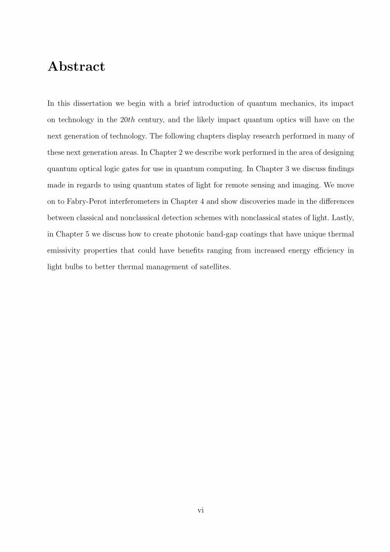
In this dissertation we begin with a brief introduction of quantum mechanics, its impact
on technology in the 20th century, and the likely impact quantum optics will have on the
next generation of technology. The following chapters display research performed in many of
these next generation areas. In Chapter 2 we describe work performed in the area of designing
quantum optical logic gates for use in quantum computing. In Chapter 3 we discuss findings
made in regards to using quantum states of light for remote sensing and imaging. We move
on to Fabry-Perot interferometers in Chapter 4 and show discoveries made in the differences
between classical and nonclassical detection schemes with nonclassical states of light. Lastly,
in Chapter 5 we discuss how to create photonic band-gap coatings that have unique thermal
emissivity properties that could have benefits ranging from increased energy efficiency in
light bulbs to better thermal management of satellites.
vi
1 Introduction
1.1 Birth of Quantum Mechanics
The birth of quantum optics can be traced back to the enigma that surrounded blackbody
radiation, which amounted to finding the relationship between heated matter and its emitted
light. A blackbody is an object which absorbs all incident electromagnetic radiation, allowing
none to pass through and none to be reflected. Having no electromagnetic radiation reflected,
including visible light, means the object appears black when not heated. However when the
object is subject to radiation its properties cause it to act as an ideal thermal radiator,
emitting on average just the same amount as it absorbs, at every wavelength, when in
thermal equilibrium with its environment.
A conflict arose in the late 19th century when physicists were struggling to create a theoret-
ical explanation of what was seen experimentally. Wilhelm Wien first derived an expression
which accurately described the behavior of a blackbody in the low wavelength limit, but
quickly failed when applied to the long wavelength regime [1]. The Wien approximation may
be written as
IW (λ, T ) =2hc2
λ5e−hcλkT , (1)
where c is the speed of light, h is Planck’s constant, k is Boltzmann’s constant, T is
temperature, and λ is wavelength.
Lord Rayleigh and Sir James derived the Rayleigh-Jeans law which agreed with blackbody
long wavelength results, but gave an answer diverging to infinity when applied to the small
wavelength regime, leading it to be dubbed “The Ultra-Violet Catastrophe” [2]. The Rayleigh-
Jeans law may be written as
IR(λ, T ) =2ckT
λ4. (2)
1
Together, the Rayleigh-Jeans law and the Wien approximation were capable of accurate
predictions when each was used in its respective region, however a complete solution derived
classically by treating light as a wave would remain elusive to theorists.
The solution to the blackbody problem came in 1899 when Planck discovered a formula
that would fit the experimental data for all wavelengths, and then set about finding a deriva-
tion for it. In the derivation he realized that he could recover his original formula if he modeled
the walls of the cavity as oscillators, and allowed their energy to be discrete integer multi-
pliers of some fundamental unit of energy which was proportional to the frequency. Planck’s
law is given as
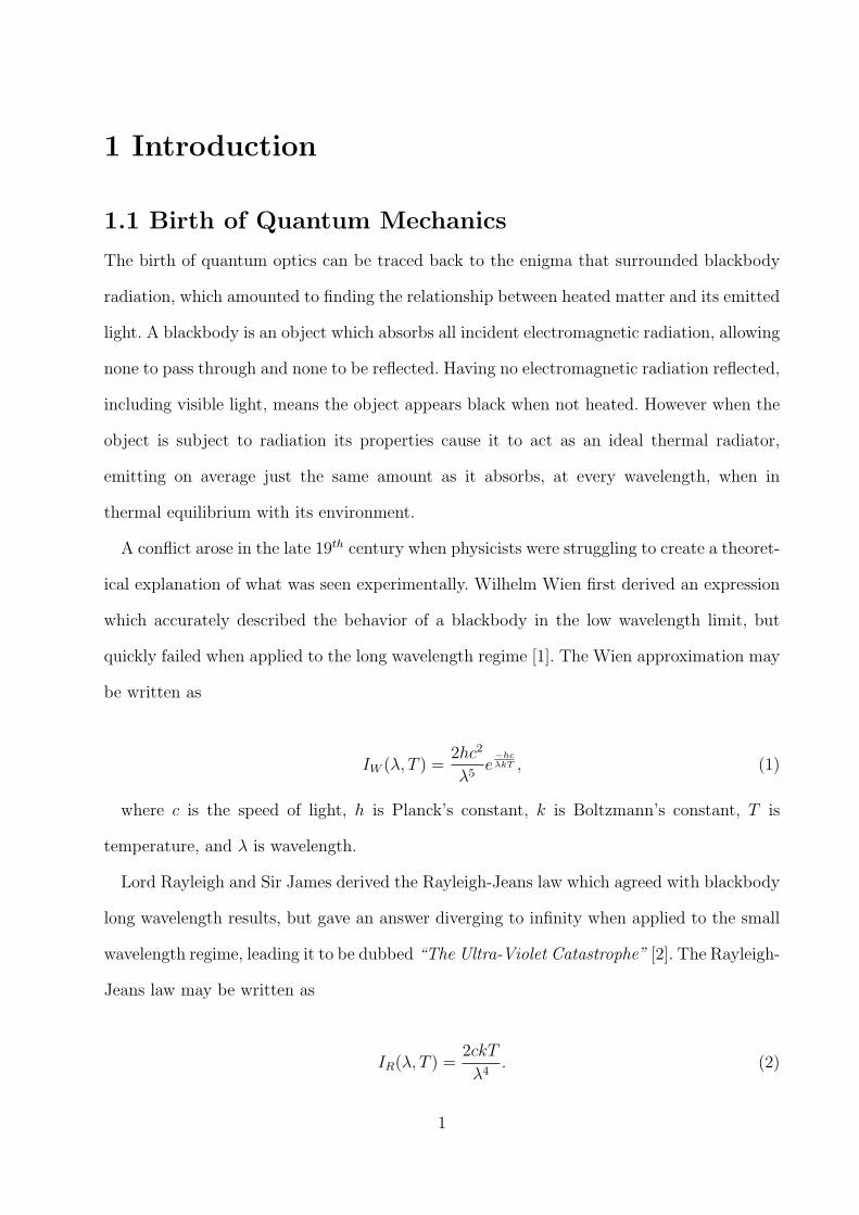
IP (λ, T ) =2hc2
λ5
1
ehc
λkT − 1(3)
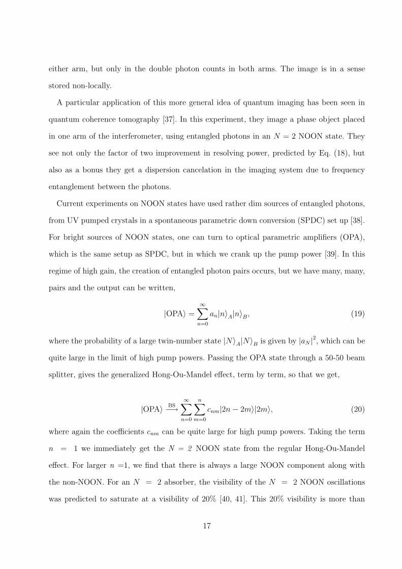
0 1.´10-6 2.´10-6 3.´10-6 4.´10-6 5.´10-60
2.´1011
4.´1011
6.´1011
8.´1011
1.´1012
1.2´1012
1.4´1012
Λ
IHΛ
,TL
FIGURE 1: Plots of Wien Approximation (dashed line), Rayleigh-Jeans law (straight line),and Planck’s Law (dotted line), versus wavelength (meters). Wien, Rayleigh-Jeans, andPlanck’s functions are in units of emitted power per unit area, per unit solid angle, perunit wavelength.
Contrary to many popular accounts, Planck did not quantize light itself, and did not truly
develop the idea of quantization as it is known in the context of quantum mechanics [3]. Six
years later, in 1905, Einstein showed that the photoelectric effect could only be explained
if light itself was quantized and treated as a particle, a photon [4]. He then described the
2
photons themselves as having discrete energy values in the form of E = hν. Planck’s theory
of discrete energy levels coupled with Einstein’s photon hypothesis led to the creation of
what we now know as the field of quantum mechanics.
“It cannot be denied that there is a broad group of facts concerning radiation, which show
that light has certain fundamental properties that can be much more readily understood from
the standpoint of Newtonian emission theory than from the standpoint of the wave theory.
It is, therefore, my opinion that the next stage of the development of theoretical physics will
bring us a theory of light which can be regarded as a kind of fusion of the wave theory and
the emission theory a profound change in our views of the nature and constitution of light
is indispensable.”
A. Einstein - 1909
1.2 The Emergence of Quantum Optics
The first 50 years of study of quantum mechanical interactions between light and matter was
considered a study of matter itself, and was typically described as atomic physics. This would
change in 1953 with the development of Microwave Amplification by Stimulated Emission
of Radiation (Maser)[5], and soon after in 1960 with Light Amplification by Stimulated
Emission of Radiation (Laser)[6]. Both the Maser and Laser are based on atomic stimulated
emission; first proposed by Einstein in 1917 to predict the ability of atoms in an excited
state to return to their ground state when stimulated by an external photon at a specific
frequency particular to the atom and the original excited energy level [7]. The research into
design and application of these new discoveries caused greater emphasis to be placed on the
study of the properties of light and the field soon came to be known as quantum optics.
1.2.1 The First Quantum Revolution
The understanding of electronic wavefunctions thanks to the development of quantum me-
chanics allowed for the complete understanding of the periodic table and all chemical reac-
3
tions. These developments were chiefly responsible for the creation of semiconductor materi-
als which in turn helped usher in what we know as the Information Age, a revolution which
has transformed the workplace, education, and communication abilities of every technologi-
cally developed society on the planet [8].
Much of the 20th century technological innovation has been focused on the attempt to
miniaturize technology; the ability to make a transistor smaller leads to cheaper and typically
faster electronics with less required resources. There are, however, limits at the bottom.
Moore’s law of computing development predicts the doubling of computer power every 18
months, leading to an exponential growth curve over the long-term. A fundamental problem
exists at the smallest scales where the laws of quantum mechanics trumps those of classical
mechanics. If the size of transistors are to be on the order of magnitude the same as hundreds
of atoms, the ability to manipulate those atoms in a precise way is needed.
The first quantum revolution brought us the semiconductor and the laser, both composed
of materials built by classical means but capable of exploiting useful quantum phenomena.
The next revolution in technology will hinge on our ability to manipulate new devices and
the way they are built at the smallest levels; a top-down design process completely in the
quantum realm.
1.2.2 The Impending Second Revolution
The newly emergent fields of quantum sensing and imaging utilize quantum entanglement —
the same subtle effects exploited in quantum information processing—to push the capability
of precision measurements and image construction using interferometers to the ultimate
quantum limit of resolution [9, 10]. Migdall at the US National Institute of Technology, for
example, has proposed and implemented a quantum optical technique for calibrating the
efficiency of photo-detectors using the temporal correlations of entangled photon pairs [11].
It was one of the first practical applications of quantum optics to optical metrology, and has
produced a technique to calibrate detectors without the need for an absolute standard.
4
These quantum effects can also be applied to increase the signal-to-noise ratio in an array of
sensors from Laser Interferometer Gravitational Wave Observatory (LIGO) to Laser Light
Detection and Ranging (LIDAR) systems, and to synchronized atomic clocks. Quantum
imaging exploits similar quantum ideas to beat the Rayleigh diffraction limit in resolution of
an imaging system, such as used in optical lithography. We present an introduction to these
exciting fields and their recent development.
Entanglement is the most profound property of quantum mechanical systems. First we
need to define entanglement. For simplification let us consider a system of two modes A and
B only. Mode A and B may describe the two spatial paths of a Mach-Zehnder interferometer
or two different polarization modes in an optical cavity. We can put a photon in either of
the modes or let them remain empty. Let us suppose a general state of mode A which is a
superposition of the two possible states, therefore we obtain α|0〉A + β|1〉A, where α and β
may be complex and |α|2 + |β|2 = 1 is required for proper normalization of the state. We also
write a superposition for a general state for mode B, i.e., γ|0〉B + δ|1〉B and |γ|2 + |δ|2 = 1.
Now consider the combined two-mode state |Ψ〉 = (|1〉A|0〉B + |0〉A|1〉B)/√
2, where either
a photon is in mode A or B. It is easy to see that this state cannot be decomposed into a
product state for mode A and mode B only, i.e., we cannot find any coefficients α, β, γ, δ such
that the equation (α|0〉A + β|1〉A) (γ|0〉B + δ|1〉B) = (|1〉A|0〉B + |0〉A|1〉B)/√
2 is satisfied.
The state|Ψ〉 is an example for a non-separable state. In general any non-separable state of
two or more systems is called entangled. Erwin Schrdinger was the first who coined the term
entanglement [12], although he is by far more prominent for his Schrdinger cat. Now we have
a proper definition for pure entangled states. But what is the definition for entangled mixed
states? Let us suppose two systems A and B that can be inn different mixed states ρAi and ρB
i
with i = 1, . . . , n. A separable mixed state may be written asρ =∑
i piρAi ⊗ ρB
i where thepi
are probabilities. It is basically a linear combination of product states. Mathematicians call
this particular sum a convex combination. Now we can define entanglement for mixed states
5
in excluding just these separable states. We say, if the bipartite system cannot be written in
the above way we call it entangled [13].
Entanglement is not necessarily a useful physical quantity. Entanglement is usually dis-
cussed together with non-local correlations. These non-local correlations can be verified by
Bell experiments [14]. For a nice review of the current status of Bell experiments see, e.g.,
Ref.[15]. The violation of a Bell inequality by a specific quantum state is an indication that
the state is able to exhibit non-local correlations. It is known that for any entangled pure
state of any number of quantum systems one may violate a generalized Bell inequality [16].
An extension of this statement for mixed entangled states has not been found. Furthermore
Werner provided in 1989 an example of non-separable mixed states that do not violate a Bell
inequality [13]. This demonstrated that the class of entangled states decomposes into states
that are entangled but do not show non-local correlations and those that are entangled and
are non-local. The state |Ψ〉 is clearly entangled but only until very recently it has been
proven in several experiments that this state violates a Bell inequality [14]. Generalizations
of this state where the single photon is replaced by N photons will play an important role
in applications described later in this chapter. That also this generalization for N photons
in either of the modes violates a Bell inequality has been proven in Ref. [17] very recently.
This shows that the connection of entanglement and non-local correlations is still a very
hot research topic. Now we will introduce a much studied and very practical application, an
optical interferometer.
1.3 Quantum Optical Interferometry
We adopt the convention that the light field always picks up a π/2 phase shift upon reflection
off of a mirror or off of a BS, and also no phase shift upon transmission through a BS. Then,
the two light fields emerging from the second BS out the upper port C are precisely π out of
phase with each other, and hence completely cancel out due to destructive interference (the
dark port). Consequently, the two light fields recombine completely in phase as they emerge
6
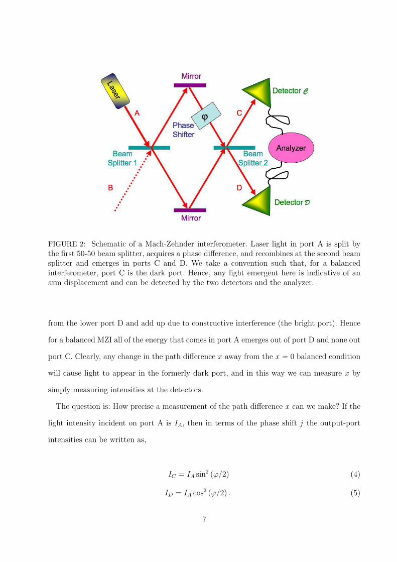
FIGURE 2: Schematic of a Mach-Zehnder interferometer. Laser light in port A is split bythe first 50-50 beam splitter, acquires a phase difference, and recombines at the second beamsplitter and emerges in ports C and D. We take a convention such that, for a balancedinterferometer, port C is the dark port. Hence, any light emergent here is indicative of anarm displacement and can be detected by the two detectors and the analyzer.
from the lower port D and add up due to constructive interference (the bright port). Hence
for a balanced MZI all of the energy that comes in port A emerges out of port D and none out
port C. Clearly, any change in the path difference x away from the x = 0 balanced condition
will cause light to appear in the formerly dark port, and in this way we can measure x by
simply measuring intensities at the detectors.
The question is: How precise a measurement of the path difference x can we make? If the
light intensity incident on port A is IA, then in terms of the phase shift j the output-port
intensities can be written as,
IC = IA sin2 (ϕ/2) (4)
ID = IA cos2 (ϕ/2) . (5)
7
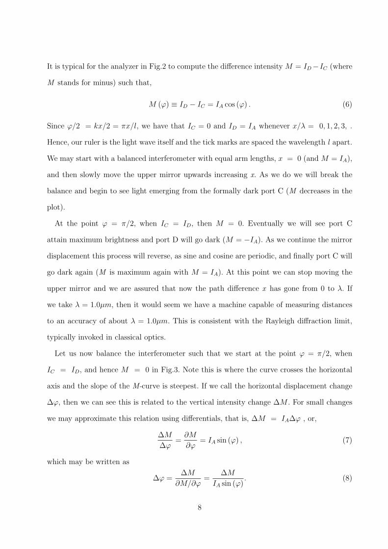
It is typical for the analyzer in Fig.2 to compute the difference intensity M = ID−IC (where
M stands for minus) such that,
M (ϕ) ≡ ID − IC = IA cos (ϕ) . (6)
Since ϕ/2 = kx/2 = πx/l, we have that IC = 0 and ID = IA whenever x/λ = 0, 1, 2, 3, .
Hence, our ruler is the light wave itself and the tick marks are spaced the wavelength l apart.
We may start with a balanced interferometer with equal arm lengths, x = 0 (and M = IA),
and then slowly move the upper mirror upwards increasing x. As we do we will break the
balance and begin to see light emerging from the formally dark port C (M decreases in the
plot).
At the point ϕ = π/2, when IC = ID, then M = 0. Eventually we will see port C
attain maximum brightness and port D will go dark (M = −IA). As we continue the mirror
displacement this process will reverse, as sine and cosine are periodic, and finally port C will
go dark again (M is maximum again with M = IA). At this point we can stop moving the
upper mirror and we are assured that now the path difference x has gone from 0 to λ. If
we take λ = 1.0µm, then it would seem we have a machine capable of measuring distances
to an accuracy of about λ = 1.0µm. This is consistent with the Rayleigh diffraction limit,
typically invoked in classical optics.
Let us now balance the interferometer such that we start at the point ϕ = π/2, when
IC = ID, and hence M = 0 in Fig.3. Note this is where the curve crosses the horizontal
axis and the slope of the M-curve is steepest. If we call the horizontal displacement change
∆ϕ, then we can see this is related to the vertical intensity change ∆M . For small changes
we may approximate this relation using differentials, that is, ∆M = IA∆ϕ , or,
∆M
∆ϕ=
∂M
∂ϕ= IA sin (ϕ) , (7)
which may be written as
∆ϕ =∆M
∂M/∂ϕ=
∆M
IA sin (ϕ). (8)
8
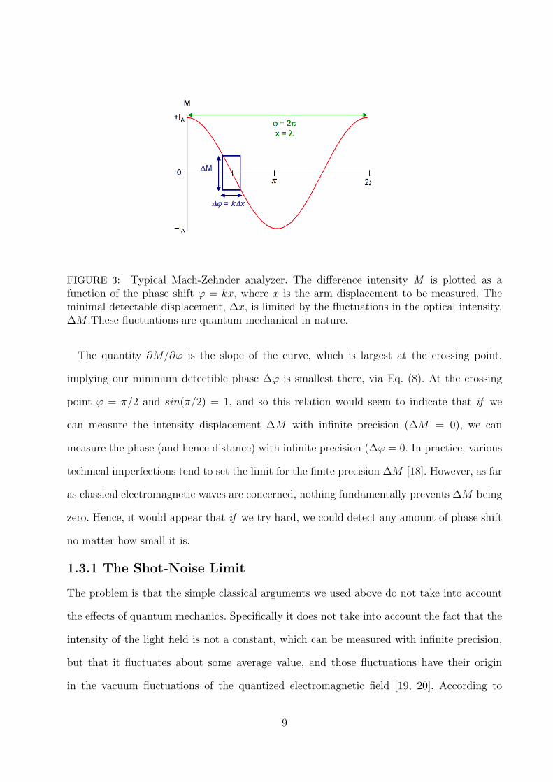
FIGURE 3: Typical Mach-Zehnder analyzer. The difference intensity M is plotted as afunction of the phase shift ϕ = kx, where x is the arm displacement to be measured. Theminimal detectable displacement, ∆x, is limited by the fluctuations in the optical intensity,∆M .These fluctuations are quantum mechanical in nature.
The quantity ∂M/∂ϕ is the slope of the curve, which is largest at the crossing point,
implying our minimum detectible phase ∆ϕ is smallest there, via Eq. (8). At the crossing
point ϕ = π/2 and sin(π/2) = 1, and so this relation would seem to indicate that if we
can measure the intensity displacement ∆M with infinite precision (∆M = 0), we can
measure the phase (and hence distance) with infinite precision (∆ϕ = 0. In practice, various
technical imperfections tend to set the limit for the finite precision ∆M [18]. However, as far
as classical electromagnetic waves are concerned, nothing fundamentally prevents ∆M being
zero. Hence, it would appear that if we try hard, we could detect any amount of phase shift
no matter how small it is.
1.3.1 The Shot-Noise Limit
The problem is that the simple classical arguments we used above do not take into account
the effects of quantum mechanics. Specifically it does not take into account the fact that the
intensity of the light field is not a constant, which can be measured with infinite precision,
but that it fluctuates about some average value, and those fluctuations have their origin
in the vacuum fluctuations of the quantized electromagnetic field [19, 20]. According to
9
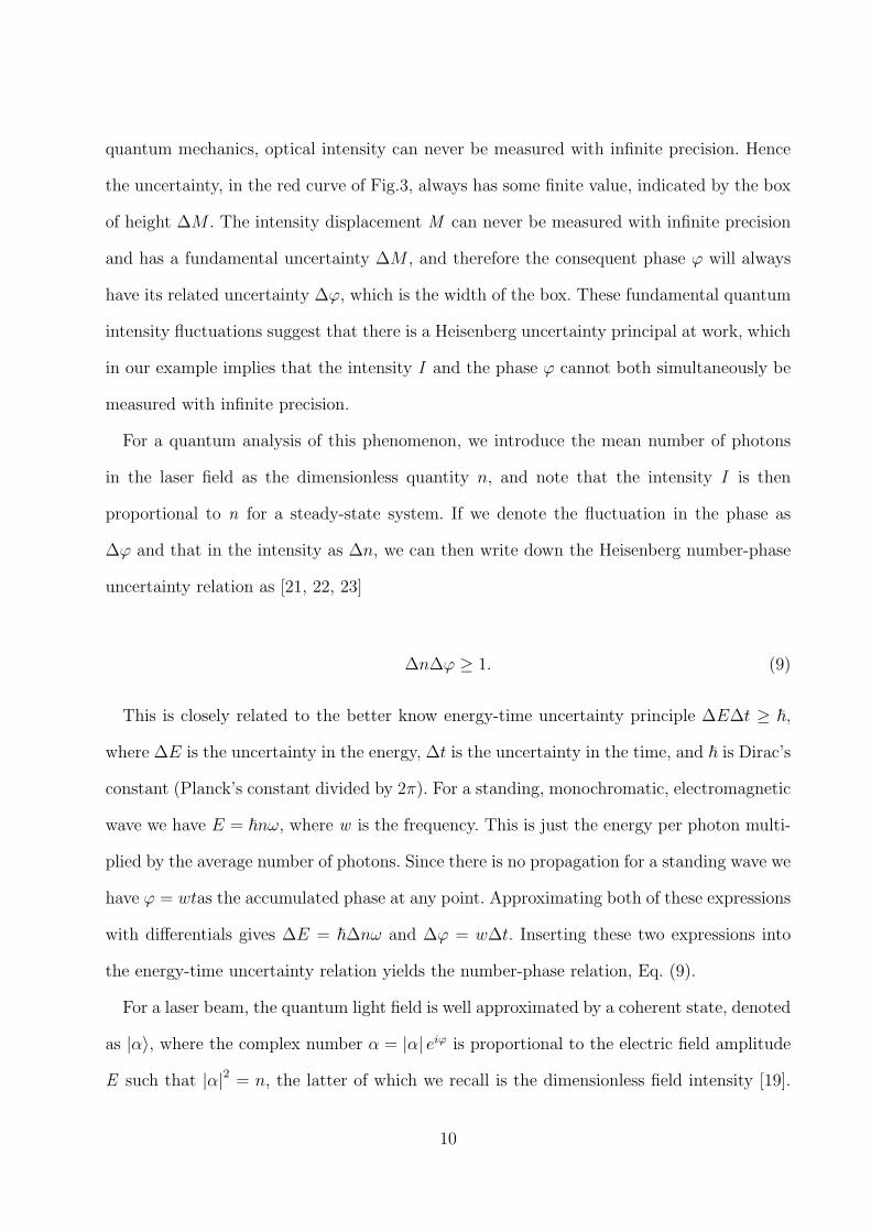
quantum mechanics, optical intensity can never be measured with infinite precision. Hence
the uncertainty, in the red curve of Fig.3, always has some finite value, indicated by the box
of height ∆M . The intensity displacement M can never be measured with infinite precision
and has a fundamental uncertainty ∆M , and therefore the consequent phase ϕ will always
have its related uncertainty ∆ϕ, which is the width of the box. These fundamental quantum
intensity fluctuations suggest that there is a Heisenberg uncertainty principal at work, which
in our example implies that the intensity I and the phase ϕ cannot both simultaneously be
measured with infinite precision.
For a quantum analysis of this phenomenon, we introduce the mean number of photons
in the laser field as the dimensionless quantity n, and note that the intensity I is then
proportional to n for a steady-state system. If we denote the fluctuation in the phase as
∆ϕ and that in the intensity as ∆n, we can then write down the Heisenberg number-phase
uncertainty relation as [21, 22, 23]
∆n∆ϕ ≥ 1. (9)
This is closely related to the better know energy-time uncertainty principle ∆E∆t ≥ ~,where ∆E is the uncertainty in the energy, ∆t is the uncertainty in the time, and ~ is Dirac’s
constant (Planck’s constant divided by 2π). For a standing, monochromatic, electromagnetic
wave we have E = ~nω, where w is the frequency. This is just the energy per photon multi-
plied by the average number of photons. Since there is no propagation for a standing wave we
have ϕ = wtas the accumulated phase at any point. Approximating both of these expressions
with differentials gives ∆E = ~∆nω and ∆ϕ = w∆t. Inserting these two expressions into
the energy-time uncertainty relation yields the number-phase relation, Eq. (9).
For a laser beam, the quantum light field is well approximated by a coherent state, denoted
as |α〉, where the complex number α = |α| eiϕ is proportional to the electric field amplitude
E such that |α|2 = n, the latter of which we recall is the dimensionless field intensity [19].
10
This is the dimensionless quantum version of the classical relation |E|2 = I = I0n. The full
dimensional form is E = E0
√n where I0 = |E0|2 = ~ω
(ε0V ), which in SI units, ~ is Dirac’s
constant, ε0 is the free-space permittivity, and V is the mode volume for the electromagnetic
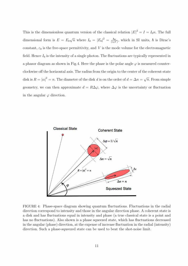
field. Hence I0 is the intensity of a single photon. The fluctuations are typically represented in
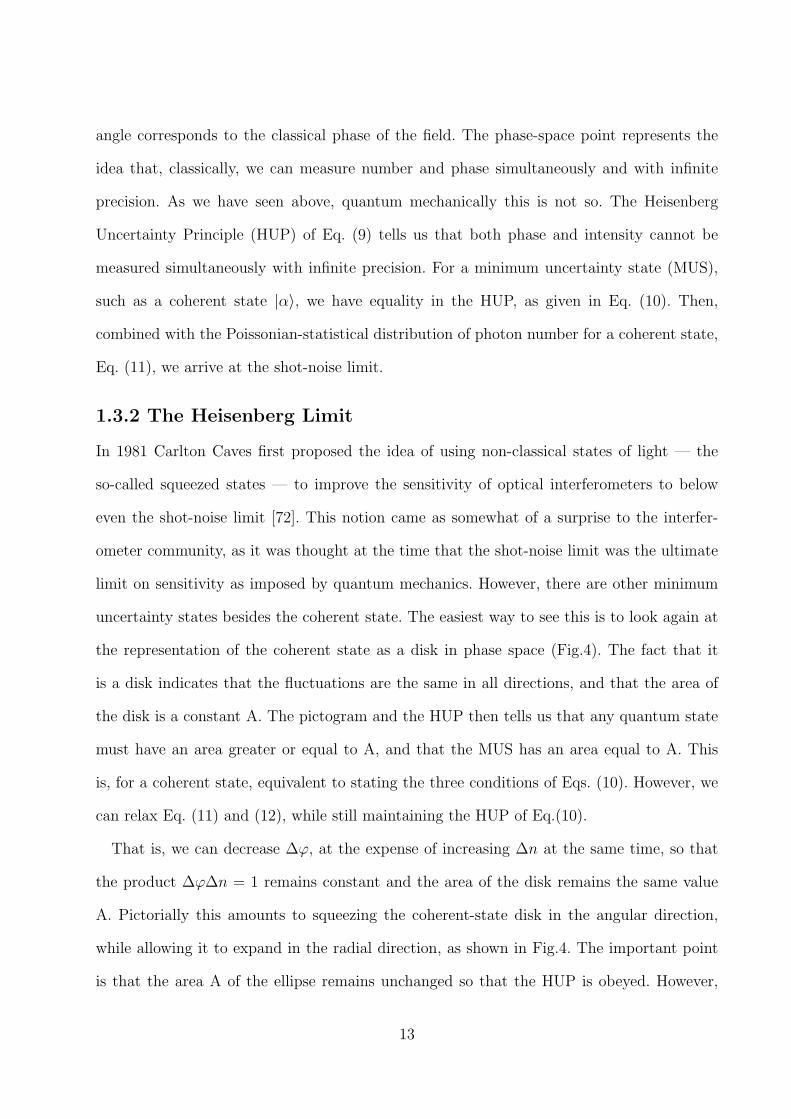
a phasor diagram as shown in Fig.4. Here the phase is the polar angle ϕ is measured counter-
clockwise off the horizontal axis. The radius from the origin to the center of the coherent-state
disk is R = |α|2 = n. The diameter of the disk d is on the order of d = ∆n =√
n. From simple
geometry, we can then approximate d = R∆ϕ, where ∆ϕ is the uncertainty or fluctuation
in the angular ϕ direction.
FIGURE 4: Phase-space diagram showing quantum fluctuations. Fluctuations in the radialdirection correspond to intensity and those in the angular direction phase. A coherent state isa disk and has fluctuations equal in intensity and phase (a true classical state is a point andhas no fluctuations). Also shown is a phase squeezed state, which has fluctuations decreasedin the angular (phase) direction, at the expense of increase fluctuation in the radial (intensity)direction. Such a phase-squeezed state can be used to beat the shot-noise limit.
11
Combining all this we arrive at the fundamental relationships between number (intensity)
and phase uncertainty for a coherent-state laser beam,
∆n∆ϕ = 1, (10)
∆n =√
n, (11)
∆ϕSNL
=1
∆n=
1√n
. (12)
The first relation, Eq.(10), tells us that we have equality in Eq.(9); that is a coherent
state is a minimum uncertainty state (MUS). Such a state saturates the Heisenberg number-
phase uncertainty relation with equality. This is the best you can do according to the laws
of quantum mechanics. The second relation, Eq. (11), describes the fact that the number
fluctuations are Poissonian with a mean of n and a deviation of ∆n =√
n, a well-known
property of the Poisson distribution and the consequent number statistics for coherent-state
laser beams [20]. Putting back the dimensions we arrive at,
∆ϕSNL =
√I0
I, (13)
which is called the shot-noise limit (SNL). The term shot noise comes from the notion that
the photon-number fluctuations arise from the scatter in arrival times of the photons at
the beam splitter, much like buckshot from a shotgun ricocheting off a metal plate. We
can also import the SNL into our classical analysis above. Consider Eq. (8), where we now
take IA = I0n, ∆M =√
I0n, and ϕ = π/2. We again recover Eq. (12) for the phase
uncertainty. Hence quantum mechanics puts a quantitative limit on the uncertainty of the
optical intensity, and that intensity reflects itself in a consequent quantitative uncertainty of
the phase measurement.
In classical electromagnetism, we can also represent a monochromatic plane wave on the
phasor diagram of Fig.4 — but instead of a disk the classical field is depicted as a point.
The radial vector to the point is proportional to the electric field amplitude E and the phase
12
angle corresponds to the classical phase of the field. The phase-space point represents the
idea that, classically, we can measure number and phase simultaneously and with infinite
precision. As we have seen above, quantum mechanically this is not so. The Heisenberg
Uncertainty Principle (HUP) of Eq. (9) tells us that both phase and intensity cannot be
measured simultaneously with infinite precision. For a minimum uncertainty state (MUS),
such as a coherent state |α〉, we have equality in the HUP, as given in Eq. (10). Then,
combined with the Poissonian-statistical distribution of photon number for a coherent state,
Eq. (11), we arrive at the shot-noise limit.
1.3.2 The Heisenberg Limit
In 1981 Carlton Caves first proposed the idea of using non-classical states of light — the
so-called squeezed states — to improve the sensitivity of optical interferometers to below
even the shot-noise limit [72]. This notion came as somewhat of a surprise to the interfer-
ometer community, as it was thought at the time that the shot-noise limit was the ultimate
limit on sensitivity as imposed by quantum mechanics. However, there are other minimum
uncertainty states besides the coherent state. The easiest way to see this is to look again at
the representation of the coherent state as a disk in phase space (Fig.4). The fact that it
is a disk indicates that the fluctuations are the same in all directions, and that the area of
the disk is a constant A. The pictogram and the HUP then tells us that any quantum state
must have an area greater or equal to A, and that the MUS has an area equal to A. This
is, for a coherent state, equivalent to stating the three conditions of Eqs. (10). However, we
can relax Eq. (11) and (12), while still maintaining the HUP of Eq.(10).
That is, we can decrease ∆ϕ, at the expense of increasing ∆n at the same time, so that
the product ∆ϕ∆n = 1 remains constant and the area of the disk remains the same value
A. Pictorially this amounts to squeezing the coherent-state disk in the angular direction,
while allowing it to expand in the radial direction, as shown in Fig.4. The important point
is that the area A of the ellipse remains unchanged so that the HUP is obeyed. However,
13
we can decrease phase uncertainty at the expense of increasing the number uncertainty.
Furthermore, it is possible to produce such squeezed states of light in the laboratory, using
nonlinear optical devices and ordinary lasers [25, 26, 27, 28].
Now the question is: What is the most uncertainty we can produce in photon number,
given that the mean photon number n is a fixed constant, and that we still want to maintain
the MUS condition— that the area of the ellipse remains a constant A. Intuitively one cannot
easily imagine a scenario where the fluctuations in the energy, ∆E = ~ω∆n, exceeds the
total energy of the laser beam, E = ~ωn. Hence the best we can hope to achieve is ∆E = E
or, canceling out some constants, ∆n = n. Inserting this expression in the HUP of Eq.(10),
we obtain what is called the Heisenberg limit:
∆ϕHL =1
n. (14)
Putting back the dimensions we get
∆ϕHL =I0
I. (15)
This is exactly the limit one gets with a rigorous derivation using squeezed light in the limit
of infinite squeezing [29, 30]. It is called the Heisenberg limit as it saturates the number-
phase HUP, and also because it can be proven that this is the best you can do in a passive
interferometer with finite average photon number n. Converting to minimum detectable
displacement we get,
∆x =λ
n= λ
I0
I. (16)
where I0 is the single photon intensity, defined above.
So far, we have considered the situation that we send light in port A and analyzed what
came out ports C and D for the MZI shown in Fig. 1. What about input port B? Classically
there is no light coming in port B, and hence it is irrelevant. But, it is not so. In his 1981
paper, Caves showed that no matter what state of the photon field you put in port A, so
14
long as you put nothing (quantum vacuum) in port B, you will always recover the SNL. In
quantum electrodynamics, even an interferometer mode with no photons in it experiences
electric field fluctuations in that mode.
In the MZI these vacuum fluctuations have another important effect; at the first BS they
enter through port B and mix with whatever is coming in port A to give the SNL in overall
sensitivity. It becomes clear then, from this result, that the next thing to try would be to
plug that unused port B with something besides vacuum. It was Caves’ idea to plug the
unused port B with squeezed light (squeezed vacuum to be exact). That, with coherent laser
light in port A as before — and in the limit of infinite squeezing — then the SNL rolls over
into the HL.
In the laboratory, however, infinite squeezing is awfully hard to come by. With current
technology [31, 32, 33], the expected situation is to sit somewhere between the shot-noise limit
(SNL) and the Heisenberg limit (HL) but a lot closer to the former than the latter. Recent
analyses by a Caltech group, on exploiting squeezed light in LIGO, indicates a potential
for about a one-order-of-magnitude improvement in a future LIGO upgrade [34]. Not the
twelve orders of magnitude that was advertised above, but enough to allow the observatory
to sample about eighty times the original volume of Space for gravitational-wave sources.
That, for LIGO, is a big deal.
In Chapter 3 we will show specific quantum states capable of achieving the Heisenberg
limit, as well as others that approach it but also perform well when undergoing photon loss.
1.4 Quantum Imaging
Quantum imaging is a new sub-field of quantum optics that exploits quantum correlations,
such as quantum entanglement of the electromagnetic field, in order to image objects with
a resolution (or other imaging criteria) that is beyond what is possible in classical optics.
Examples of quantum imaging are quantum ghost imaging, quantum lithography, and sub-
Rayleigh imaging [74, 75]. In 2000 it was pointed out that NOON states had the capability
15
to beat the Rayleigh diffraction limit by a factor of N. This super resolution feature is due
to the high-frequency oscillations of the NOON state in the interferometer, as illustrated in
Fig. 4. For the quantum lithography application, the idea is to realize that if one has an
N-photon absorbing material, used as a lithographic resist, then these high-frequency oscil-
lations are written onto the material in real space and are not just a trace on an oscilloscope.
Mathematically, the N -photon absorption and the N-photon detection process have a similar
structure, that is,
〈NOON| (a†)N(a)N |NOON〉 = 1 + cos (Nϕ) , (17)
where a and a†are the mode annihilation and creation operators. From Fig. 4, we see in the
green curve this oscillates N times faster than if we were using single photons, or coherent
light, as in the red curve. Recall that, for our MZI, we have ϕ = kx = 2πx/λ, where x is
the displacement between the two arms. For lithography x is also the distance measured on
the photographic plate or lithographic resist. If we compare the classical resolution to the
NOON resolution we may write, ϕNOON = Nϕclassical, which we can solve for,
λNOON =λclassical
N. (18)
Written this way, we can say the effective wavelength of the N photons bundled together
N at a time into the NOON state is N times smaller than the classical wavelength. This is
another way to understand the super-resolution effect. The N entangled photons conspire
to behave as a single classical photon of a wavelength smaller by a factor of N [35]. Since
the Rayleigh diffraction limit for lithography is couched in terms of the minimal resolvable
distance ∆x = λ classical, then we have ∆xN00N = λN00N = λclasssical/N .
Another interesting application is so-called ghost imaging. This effect exploits the temporal
and spatial correlations of photon pairs, also from spontaneous parametric down conversion,
to image an object in one branch of the interferometer by looking at correlations in the
coincidence counts of the photons [36]. There is no image in the single-photon counts in
16
either arm, but only in the double photon counts in both arms. The image is in a sense
stored non-locally.
A particular application of this more general idea of quantum imaging has been seen in
quantum coherence tomography [37]. In this experiment, they image a phase object placed
in one arm of the interferometer, using entangled photons in an N = 2 NOON state. They
see not only the factor of two improvement in resolving power, predicted by Eq. (18), but
also as a bonus they get a dispersion cancelation in the imaging system due to frequency
entanglement between the photons.
Current experiments on NOON states have used rather dim sources of entangled photons,
from UV pumped crystals in a spontaneous parametric down conversion (SPDC) set up [38].
For bright sources of NOON states, one can turn to optical parametric amplifiers (OPA),
which is the same setup as SPDC, but in which we crank up the pump power [39]. In this
regime of high gain, the creation of entangled photon pairs occurs, but we have many, many,
pairs and the output can be written,
|OPA〉 =∞∑
n=0
an|n〉A|n〉B, (19)
where the probability of a large twin-number state |N〉A|N〉B is given by |aN |2, which can be
quite large in the limit of high pump powers. Passing the OPA state through a 50-50 beam
splitter, gives the generalized Hong-Ou-Mandel effect, term by term, so that we get,
|OPA〉 BS−→∞∑
n=0
n∑m=0
cnm|2n− 2m〉|2m〉, (20)
where again the coefficients cnm can be quite large for high pump powers. Taking the term
n = 1 we immediately get the N = 2 NOON state from the regular Hong-Ou-Mandel
effect. For larger n =1, we find that there is always a large NOON component along with
the non-NOON. For an N = 2 absorber, the visibility of the N = 2 NOON oscillations
was predicted to saturate at a visibility of 20% [40, 41]. This 20% visibility is more than
17
enough to exploit for lithography and imaging, and has recently been measured in a recent
experiment in the group of DeMartini in Rome [42], in collaboration with our activity at
Louisiana State University.
1.5 Quantum Computing
The main focus within the field of quantum technologies has undoubtedly been quantum
computing. Starting in 1994, with Peter Shor’s discovery that quantum computers could
break public-key cryptography systems in polynomial time rather than the conventional
exponential time [43], researchers have focused their attention on how to build both the
hardware and software for such a machine. While the idea of encoding information with the
rules of quantum mechanics had been around since 1984 [44], Shor’s paper was the first to
show how to decode classically encrypted material relatively quickly by nonclassical means;
a revolutionary idea that has major security and national intelligence implications. If Shor’s
algorithm was implemented by a hostile entity, private and commercial internet traffic would
become very vulnerable to eavesdropping and disruption. Understandably, research dollars
have poured in from intelligence agencies hoping to claim such power as their own.
There are numerous competing methods for building the physical implementation of a
quantum computer; they include: superconductors, trapped ions, optical lattices, quantum
dots, nuclear magnetic resonance (NMR), quantum optics, Bose-Einstein condensates, and
even a diamond-based implementation [45]. In this thesis we will restrict ourselves to matters
associated with quantum optics based computing. In this picture, a quantum computer would
ideally be built with single photon on-demand sources, high efficiency single photon detec-
tors, low-loss scalable optical circuits for photons to traverse, and minimal environmental
interaction.
Any computer, be it classical or nonclassical, needs a mechanism by which to manipulate
data. This mechanism is termed a logic gate; a conditional set of instructions that changes
input data into desired output data in the course of performing a task. For classical com-
18
puters logic gates are encoded electronically using transistors, a method not suitable for our
nonclassical computer. A quantum optical logic gate needs to follow the rules of quantum
mechanics, meaning it must evolve in a unitary fashion and in such a manner as to not
introduce decoherence to the system. Any device that behaves in a unitary fashion may
be mathematically expressed as a unitary matrix, which may then in turn be physically
expressed by a series of optical elements including interferometers and beam-splitters. In
Chapter 2 we will explore the process behind the discovery of such matrices, and how they
are optimized for maximum efficiency. The creation and optimization of unitary matrices
which represent physical quantum logic gates lies at the very heart of the ongoing task to
create a scalable, fault-tolerant quantum computer.
19
2 Engineering Quantum Optical Logic GatesFor Quantum Computing
2.1 Linear Optical Logic Gates
Linear optics has become a leading contender for the method of choice in building a quantum
computer, alongside super-conducting quantum dots and ion trapping, in large part due to
the work of Knill, Laflamme and Milburn (KLM)[46] and their scheme for designing non-
determinate quantum logic gates using projective measurement. Their scheme was the first
to show how one can build elementary quantum gates with only linear optical elements, a
task much easier than using nonlinear optical elements and their demand of large photon
flux to produce a relatively small amount of output. The tradeoff in this scheme is that the
gates can only be made with a certain probability of correctly working, i.e., they are non-
deterministic. Therefore, the main goal in designing a linear optical logic gate is to figure
out how to achieve a design with the highest success probability possible, and do so while
maintaining a high level of fidelity.
A linear optical quantum state generator (LOQSG) can simply be viewed as a unitary
operation which transforms an input state into a desired output state. The main aim of
designing a LOQSG is to obtain a unitary matrix which accomplishes the desired trans-
formation and whose elements can then be realized with linear optical devices within the
mentioned KLM scheme, such as beamsplitters and phase shifters [47, 48]. In this chapter we
will describe work done using genetic algorithms with a simulated annealing process that was
used to find and optimize suitable unitary matrices. We begin by first testing our method
on the non-linear sign gate, chosen because its maximum success probability is known to be
1/4 without any special feed-forward information [49, 50]. We then attempt to obtain a new
global maximum for success probability with the case of the controlled-sign (CZ) gate, as it
is as of yet theoretically unknown what the maximum is.
20
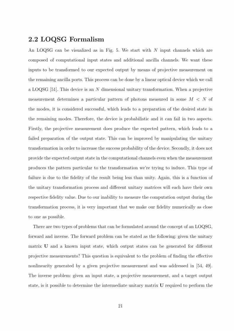
2.2 LOQSG Formalism
An LOQSG can be visualized as in Fig. 5. We start with N input channels which are
composed of computational input states and additional ancilla channels. We want these
inputs to be transformed to our expected output by means of projective measurement on
the remaining ancilla ports. This process can be done by a linear optical device which we call
a LOQSG [51]. This device is an N dimensional unitary transformation. When a projective
measurement determines a particular pattern of photons measured in some M < N of
the modes, it is considered successful, which leads to a preparation of the desired state in
the remaining modes. Therefore, the device is probabilistic and it can fail in two aspects.
Firstly, the projective measurement does produce the expected pattern, which leads to a
failed preparation of the output state. This can be improved by manipulating the unitary
transformation in order to increase the success probability of the device. Secondly, it does not
provide the expected output state in the computational channels even when the measurement
produces the pattern particular to the transformation we’re trying to induce. This type of
failure is due to the fidelity of the result being less than unity. Again, this is a function of
the unitary transformation process and different unitary matrices will each have their own
respective fidelity value. Due to our inability to measure the computation output during the
transformation process, it is very important that we make our fidelity numerically as close
to one as possible.
There are two types of problems that can be formulated around the concept of an LOQSG,
forward and inverse. The forward problem can be stated as the following: given the unitary
matrix U and a known input state, which output states can be generated for different
projective measurements? This question is equivalent to the problem of finding the effective
nonlinearity generated by a given projective measurement and was addressed in [54, 49].
The inverse problem: given an input state, a projective measurement, and a target output
state, is it possible to determine the intermediate unitary matrix U required to perform the
21
FIGURE 5: An generalized Linear Optical Quantum State Generator. It exploits linearoperations, which eventually can be represented as a unitary transformation, and projectivemeasurements to convert an input state into a target output state
necessary unitary transformation of the LOQSG? In the following work we developed ways
to solve the second problem numerically using an annealing genetic algorithm that would
identify an optimum Unitary transformation matrix which would simultaneously have the
highest possible success probability while maintaining a fidelity very close to one.
2.3 Unitary Transformation Process
The linear optical measurement-assisted transformation works as follows. We start from
a computational input state |ψCin〉 of N − M modes, combined with ancilla state |ψA
in〉 in
M modes so that the input state is written as |Ψin〉 = |ψCin〉 ⊗ |ψA
in〉. The optical device
induces a unitary transformation U of the |Ψin〉 state. After that a number-resolving photo-
counting measurement is applied to the M ancilla modes. The latter is formally described
by a Kraus POVM operator in ancilla modes P = |vacuumA〉〈kN−M+1, kN−M+2, ..., kN−M |.The resulting transformation of the computational state |ψC
in〉 is a contraction quantum map
|ψCout〉 = A|ψC
in〉/‖ψCin‖ [52], where the action of the linear operator A is given by the following
projection
A|ψCin〉 = 〈kN−M+1, kN−M+2, ..., kN−M |U|ψC
in〉 ⊗ |ψAin〉. (21)
In the context of the LOQSG problem, operator A contains all the information of state
transformation.
22
The optical interferometer is considered formally as canonical transformation of creation
operators a†i → Uija†j induced by an N × N unitary matrix U . If the input state is given
in the Fock representation as |Ψin〉 = |n1, n2, ..., nN−M〉 ⊗ |nN−M+1, ..., nN〉, the unitary
transformation U in equation (21) is given by
|Φout〉 = U|Ψin〉 =N∏
i=1
1√ni!
(∑j=1
Ui,ja†j
)ni
|0〉. (22)
Transformation of Eq. (22) is a high-dimensional irreducible representation of the N × N
matrix of the optical transformation U [53]. In Fock representation, matrix elements of
〈n|U |n′〉 are calculated as permanents of matrix U [51].
Now we specify main properties of the Eq. (21) relevant to numerical implementation of
the optimization algorithm. In the computational Fock basis |nc〉, the Eq. (21) is described
by matrix Anc1,nc
2= 〈nc
1|A|nc2〉, which is simply a submatrix of 〈n|U |n〉. Thus A has a form
of a set of polynomial functions in variables uij, computed using Eq. (22), so that Eq. (22)
specifies an explicit algebraic form of dependence of A on U . If the total number of measured
photons in ancilla modes∑N
i=N−M+1 ki is the same as the number of input ancilla photons
∑Ni=N−M+1 ni, then Eq. (21) leaves the number of computational photons invariant. Since
the dual-rail computational basis is just a subset of all possible states in the computational
modes, the transformation matrix Anc1,nc
2is in general a non-square matrix, mapping the
Hilbert space of the computation basis to a larger Hilbert space. For example, Anc1,nc
2for the
CS is a 10× 4 matrix.
2.4 Fidelity and Success Probability Definitions
We now introduce the notion of operational fidelity of a transformation, which in general
differs from the common measure of fidelity for a state transformation. From a physical point
of view, the transformation A satisfies a 100% fidelity criteria if it is proportional to the tar-
get transformation operation AT , i.e., A ≡ αAT , where α is an arbitrary complex number.
Since the target transformation is supposed to be a unitary gate, i.e., ATTarATar = I. The op-
23
erational fidelity condition also requires that desired transformation A satisfies operational
unitarity condition AT A = SI, where S = |α|2 is the success probability of the transfor-
mation [54]. To formulate an algebraic estimate for the accuracy of the transformation, we
consider complex rays βA and αAT as elements of complex projective space. The measure
of closeness of elements in such a projective space is given by the Fubini-Study distance
γ(u) = arccos
√〈A|ATar〉〈ATar|A〉〈A|A〉〈ATar|ATar〉
, (23)
where the Hermitian inner product is 〈A|B〉 ≡ Tr(AB†)/Dc, and Dc is the dimensionality
of computational space.
In the numerical implementation of the optimization we used a nonsingular variable F =
cos γ2, which we will refer to as fidelity in the rest of the chapter.
The success probability S of the transformation depends on the initial state |ψc〉 . The up-
per bound of S is determined by the operator norm ‖A‖Max = Max(〈ψc|A†A|ψc〉/〈ψc|ψc〉),and correspondingly the lower bound of S is ‖A‖Min = Min(〈ψc|A†A|ψc〉/〈ψc|ψc〉). As
a measurement of the success probability, we use the Hilbert-Schmidt norm ‖A‖(HS) =√Tr(A†A)/Dc. It is easy to verify that ‖A‖Min ≤ ‖A‖(HS) ≤ ‖A‖Max. As fidelity F → 1,
‖A‖Min/‖A‖Max → 1 and S becomes a well defined parameter equal to ‖A‖(HS). We will
refer to the Hilbert-Schmidt norm ‖A‖(HS) as success probability, keeping in mind that such
a definition may not correspond to a success probability of transformation of specific state
initial state.
2.5 The NS and CS Gates
As an example, let us consider first the nonlinear sign (NS) gate. The NS gate with 2 ancilla
modes is as follows
α|010〉+ β|110〉+ γ|210〉 −→ α|010〉+ β|110〉 − γ|210〉 (24)
24
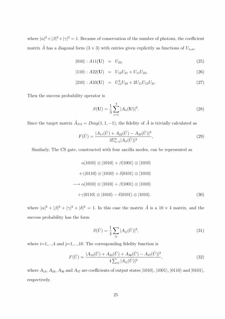
where |α|2 + |β|2 + |γ|2 = 1. Because of conservation of the number of photons, the coefficient
matrix A has a diagonal form (3× 3) with entries given explicitly as functions of Un,m.
|010〉 : A11(U) = U22, (25)
|110〉 : A22(U) = U12U21 + U11U22, (26)
|210〉 : A33(U) = U211U22 + 2U11U12U21. (27)
Then the success probability operator is
S(U) =1
3
3∑i=1
|Aii(U)|2. (28)
Since the target matrix ANS = Diag(1, 1,−1), the fidelity of A is trivially calculated as
F (U) =|A11(U) + A22(U)− A33(U)|2
3Σ3i=1|Aii(U)|2 , (29)
Similarly, The CS gate, constructed with four ancilla modes, can be represented as
α|1010〉 ⊗ |1010〉+ β|1001〉 ⊗ |1010〉
+γ|0110〉 ⊗ |1010〉+ δ|0101〉 ⊗ |1010〉
−→ α|1010〉 ⊗ |1010〉+ β|1001〉 ⊗ |1010〉
+γ|0110〉 ⊗ |1010〉 − δ|0101〉 ⊗ |1010〉. (30)
where |α|2 + |β|2 + |γ|2 + |δ|2 = 1. In this case the matrix A is a 10 × 4 matrix, and the
success probability has the form
S(U) =1
4
∑ij
|Aij(U)|2, (31)
where i=1,...,4 and j=1,...,10. The corresponding fidelity function is
F (U) =|A13(U) + A24(U) + A36(U)− A47(U)|2
4∑
ij |Aij(U)|2 , (32)
where A13, A24, A36 and A47 are coefficients of output states |1010〉, |1001〉, |0110〉 and |0101〉,respectively.
25
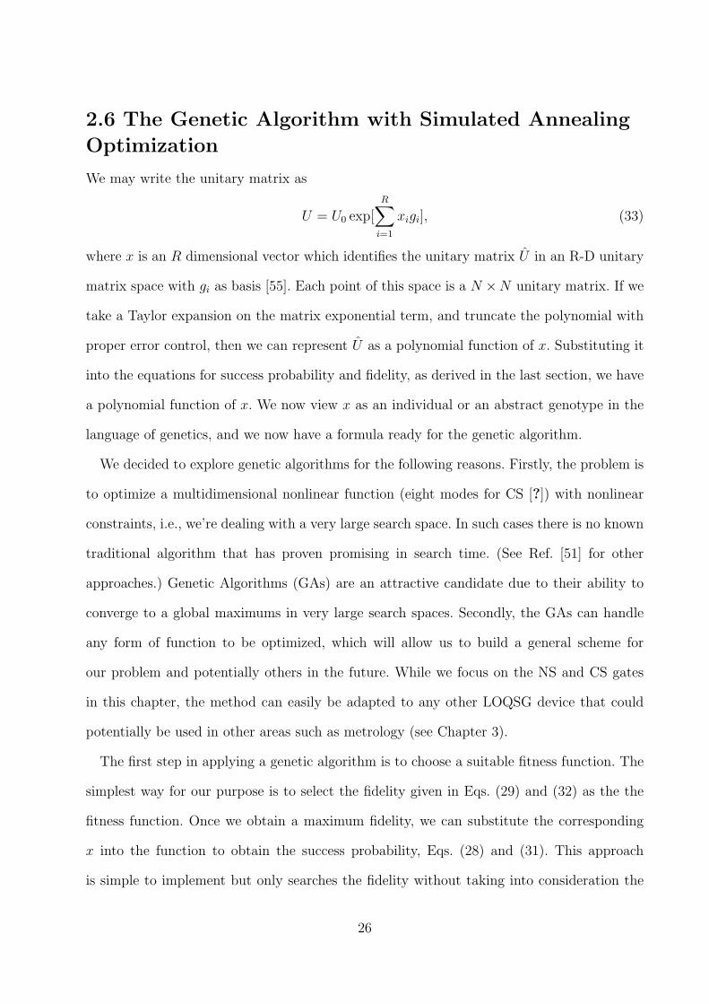
2.6 The Genetic Algorithm with Simulated Annealing
Optimization
We may write the unitary matrix as
U = U0 exp[R∑
i=1
xigi], (33)
where x is an R dimensional vector which identifies the unitary matrix U in an R-D unitary
matrix space with gi as basis [55]. Each point of this space is a N ×N unitary matrix. If we
take a Taylor expansion on the matrix exponential term, and truncate the polynomial with
proper error control, then we can represent U as a polynomial function of x. Substituting it
into the equations for success probability and fidelity, as derived in the last section, we have
a polynomial function of x. We now view x as an individual or an abstract genotype in the
language of genetics, and we now have a formula ready for the genetic algorithm.
We decided to explore genetic algorithms for the following reasons. Firstly, the problem is
to optimize a multidimensional nonlinear function (eight modes for CS [?]) with nonlinear
constraints, i.e., we’re dealing with a very large search space. In such cases there is no known
traditional algorithm that has proven promising in search time. (See Ref. [51] for other
approaches.) Genetic Algorithms (GAs) are an attractive candidate due to their ability to
converge to a global maximums in very large search spaces. Secondly, the GAs can handle
any form of function to be optimized, which will allow us to build a general scheme for
our problem and potentially others in the future. While we focus on the NS and CS gates
in this chapter, the method can easily be adapted to any other LOQSG device that could
potentially be used in other areas such as metrology (see Chapter 3).
The first step in applying a genetic algorithm is to choose a suitable fitness function. The
simplest way for our purpose is to select the fidelity given in Eqs. (29) and (32) as the the
fitness function. Once we obtain a maximum fidelity, we can substitute the corresponding
x into the function to obtain the success probability, Eqs. (28) and (31). This approach
is simple to implement but only searches the fidelity without taking into consideration the
26
success probability. Knowing the fidelity must be close to one to have a reliable result, we can
consider fidelity as being the chief constraint and success probability as the fitness function.
There are many different types of constrained genetic algorithms [56], one of them being the
simulated annealing method [58]. Using this particular method, we need to reformulate the
fitness function to contain the constraint. The new fitness function can be written as
φ(x) = α(F (x), T )S(x), (34)
with
α(F (x), T ) = e−(1−F (x))/T , (35)
where F (x) is the fidelity function used as the constraint. The second parameter, referred to
as the temperature T , is a function of the running time of the algorithm; T tends to 0 (or
very small values numerically) as execution proceeds. S(x) is the success probability, and
α(F (x), T ) acts as a penalty so that the constraint can eventually be satisfied. When the
GA begins, we want the penalty to be small, i.e., α ≈ 1, so that the algorithm can search a
larger space to find the global maximum. When T is large, which happens at the beginning
of the execution, then α ≈ 1. As time goes on, T → 0, then α → 0. It means the fitness
tends to zero unless the constraint is satisfied, i.e., F (x) ≈ 1. Therefore, at the end of the
GA run, we can obtain the optimized success probability with a fidelity of one. The details
of this simulated annealing genetic algorithm are described in Ref. [58].
The annealing genetic algorithm provides a way to search the global maximum of suc-
cess probability of a LOQSG system and guarantees that fidelity is equal, or numerically
approximate to one at the same time. The main disadvantage of this particular approach is
the efficiency delicately depends on the choice of the temperature annealing rate [56]. In the
following section, we investigate this problem using the NS gate as an example.
We used the MIT Evolutionary Library (EOlib) [58] as the source for our genetic algo-
rithm framework. In the case of the NS gate, we compared efficiency for different approaches
27
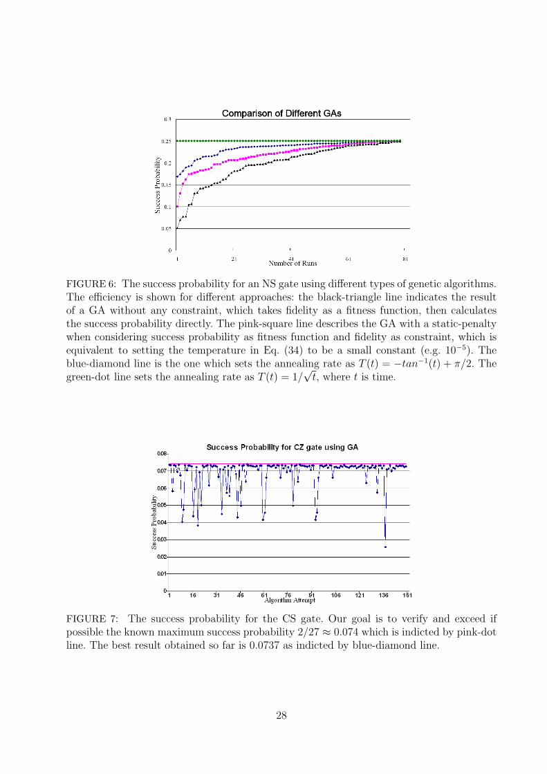
FIGURE 6: The success probability for an NS gate using different types of genetic algorithms.The efficiency is shown for different approaches: the black-triangle line indicates the resultof a GA without any constraint, which takes fidelity as a fitness function, then calculatesthe success probability directly. The pink-square line describes the GA with a static-penaltywhen considering success probability as fitness function and fidelity as constraint, which isequivalent to setting the temperature in Eq. (34) to be a small constant (e.g. 10−5). Theblue-diamond line is the one which sets the annealing rate as T (t) = −tan−1(t) + π/2. Thegreen-dot line sets the annealing rate as T (t) = 1/
√t, where t is time.
FIGURE 7: The success probability for the CS gate. Our goal is to verify and exceed ifpossible the known maximum success probability 2/27 ≈ 0.074 which is indicted by pink-dotline. The best result obtained so far is 0.0737 as indicted by blue-diamond line.
28
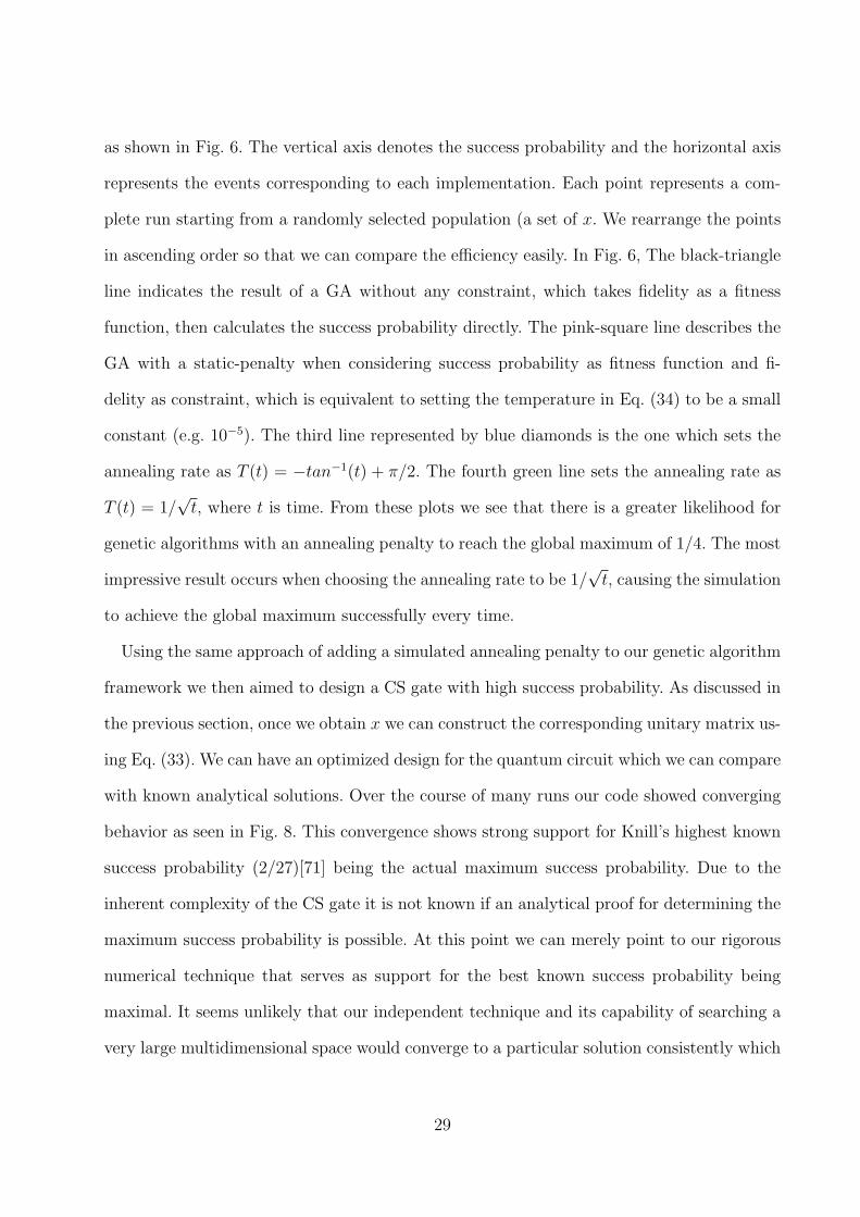
as shown in Fig. 6. The vertical axis denotes the success probability and the horizontal axis
represents the events corresponding to each implementation. Each point represents a com-
plete run starting from a randomly selected population (a set of x. We rearrange the points
in ascending order so that we can compare the efficiency easily. In Fig. 6, The black-triangle
line indicates the result of a GA without any constraint, which takes fidelity as a fitness
function, then calculates the success probability directly. The pink-square line describes the
GA with a static-penalty when considering success probability as fitness function and fi-
delity as constraint, which is equivalent to setting the temperature in Eq. (34) to be a small
constant (e.g. 10−5). The third line represented by blue diamonds is the one which sets the
annealing rate as T (t) = −tan−1(t) + π/2. The fourth green line sets the annealing rate as
T (t) = 1/√
t, where t is time. From these plots we see that there is a greater likelihood for
genetic algorithms with an annealing penalty to reach the global maximum of 1/4. The most
impressive result occurs when choosing the annealing rate to be 1/√
t, causing the simulation
to achieve the global maximum successfully every time.
Using the same approach of adding a simulated annealing penalty to our genetic algorithm
framework we then aimed to design a CS gate with high success probability. As discussed in
the previous section, once we obtain x we can construct the corresponding unitary matrix us-
ing Eq. (33). We can have an optimized design for the quantum circuit which we can compare
with known analytical solutions. Over the course of many runs our code showed converging
behavior as seen in Fig. 8. This convergence shows strong support for Knill’s highest known
success probability (2/27)[71] being the actual maximum success probability. Due to the
inherent complexity of the CS gate it is not known if an analytical proof for determining the
maximum success probability is possible. At this point we can merely point to our rigorous
numerical technique that serves as support for the best known success probability being
maximal. It seems unlikely that our independent technique and its capability of searching a
very large multidimensional space would converge to a particular solution consistently which
29
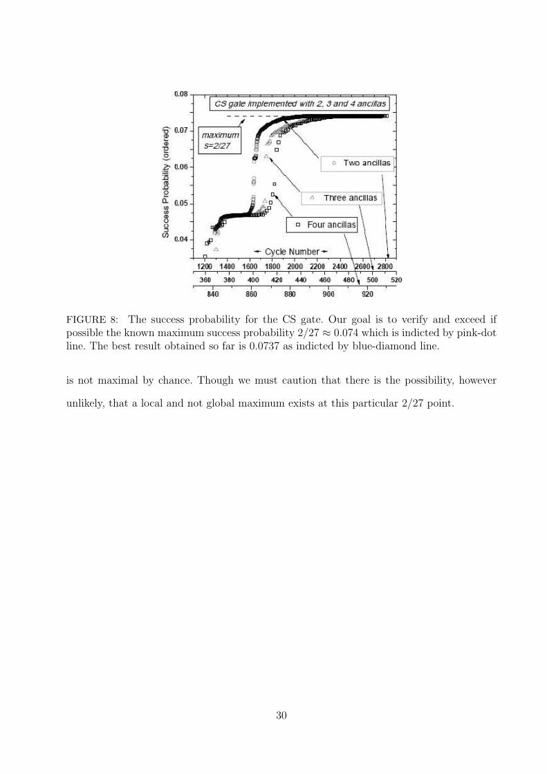
FIGURE 8: The success probability for the CS gate. Our goal is to verify and exceed ifpossible the known maximum success probability 2/27 ≈ 0.074 which is indicted by pink-dotline. The best result obtained so far is 0.0737 as indicted by blue-diamond line.
is not maximal by chance. Though we must caution that there is the possibility, however
unlikely, that a local and not global maximum exists at this particular 2/27 point.
30
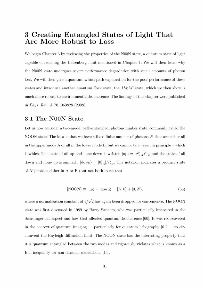
3 Creating Entangled States of Light ThatAre More Robust to Loss
We begin Chapter 3 by reviewing the properties of the N00N state, a quantum state of light
capable of reaching the Heisenberg limit mentioned in Chapter 1. We will then learn why
the N00N state undergoes severe performance degradation with small amounts of photon
loss. We will then give a quantum which-path explanation for the poor performance of these
states and introduce another quantum Fock state, the M&M ′ state, which we then show is
much more robust to environmental decoherence. The findings of this chapter were published
in Phys. Rev. A 78, 063828 (2008).
3.1 The N00N State
Let us now consider a two-mode, path-entangled, photon-number state, commonly called the
NOON state. The idea is that we have a fixed finite number of photons N that are either all
in the upper mode A or all in the lower mode B, but we cannot tell—even in principle—which
is which. The state of all up and none down is written |up〉 = |N〉A|0〉B and the state of all
down and none up is similarly |down〉 = |0〉A|N〉B. The notation indicates a product state
of N photons either in A or B (but not both) such that
|NOON〉 ≡ |up〉+ |down〉 = |N, 0〉+ |0, N〉. (36)
where a normalization constant of 1/√
2 has again been dropped for convenience. The NOON
state was first discussed in 1989 by Barry Sanders, who was particularly interested in the
Schrdinger-cat aspect and how that affected quantum decoherence [60]. It was rediscovered
in the context of quantum imaging — particularly for quantum lithography [61] — to cir-
cumvent the Rayleigh diffraction limit. The NOON state has the interesting property that
it is quantum entangled between the two modes and rigorously violates what is known as a
Bell inequality for non-classical correlations [14].
31
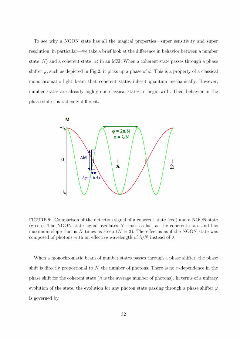
To see why a NOON state has all the magical properties—super sensitivity and super
resolution, in particular—we take a brief look at the difference in behavior between a number
state |N〉 and a coherent state |α〉 in an MZI. When a coherent state passes through a phase
shifter ϕ, such as depicted in Fig.2, it picks up a phase of ϕ. This is a property of a classical
monochromatic light beam that coherent states inherit quantum mechanically. However,
number states are already highly non-classical states to begin with. Their behavior in the
phase-shifter is radically different.
FIGURE 9: Comparison of the detection signal of a coherent state (red) and a NOON state(green). The NOON state signal oscillates N times as fast as the coherent state and hasmaximum slope that is N times as steep (N = 3). The effect is as if the NOON state wascomposed of photons with an effective wavelength of λ/N instead of λ
When a monochromatic beam of number states passes through a phase shifter, the phase
shift is directly proportional to N, the number of photons. There is no n-dependence in the
phase shift for the coherent state (n is the average number of photons). In terms of a unitary
evolution of the state, the evolution for any photon state passing through a phase shifter ϕ
is governed by
32
U (ϕ) ≡ exp (iϕn) (37)
where n is the photon number operator. The phase shift operator can be shown to have
the following two different effects on coherent vs. number states [20]
Uϕ|α〉 =∣∣eiϕα
⟩, (38)
Uϕ|N〉 = eiNϕ|N〉. (39)
Notice that the phase shift for the coherent state is independent of number, but that there
is an N dependence in the exponential for the number state. The number state then evolves
in phase N-times more rapidly than the coherent state. After the phase shifter the NOON
state evolves into,
|N, 0〉+ |0, N〉 → eiNϕ|N, 0〉+ |0, N〉, (40)
which is the origin of the quantum improvement phase sensitivity. If we now carry out
an N-photon detecting analyzer (still different from the conventional difference intensity
measurement), we obtain
MNOON (ϕ) = IA cos (Nϕ) , (41)
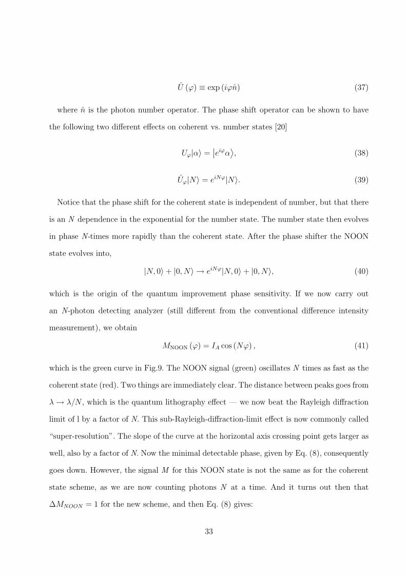
which is the green curve in Fig.9. The NOON signal (green) oscillates N times as fast as the
coherent state (red). Two things are immediately clear. The distance between peaks goes from
λ → λ/N , which is the quantum lithography effect — we now beat the Rayleigh diffraction
limit of l by a factor of N. This sub-Rayleigh-diffraction-limit effect is now commonly called
“super-resolution”. The slope of the curve at the horizontal axis crossing point gets larger as
well, also by a factor of N. Now the minimal detectable phase, given by Eq. (8), consequently
goes down. However, the signal M for this NOON state is not the same as for the coherent
state scheme, as we are now counting photons N at a time. And it turns out then that
∆MNOON = 1 for the new scheme, and then Eq. (8) gives:
33
∆ϕNOON = 1/N, (42)
which is precisely the Heisenberg limit of Eq. (14). This Heisenberg limit, or the beating of
the shot-noise limit, is now commonly called super sensitivity.
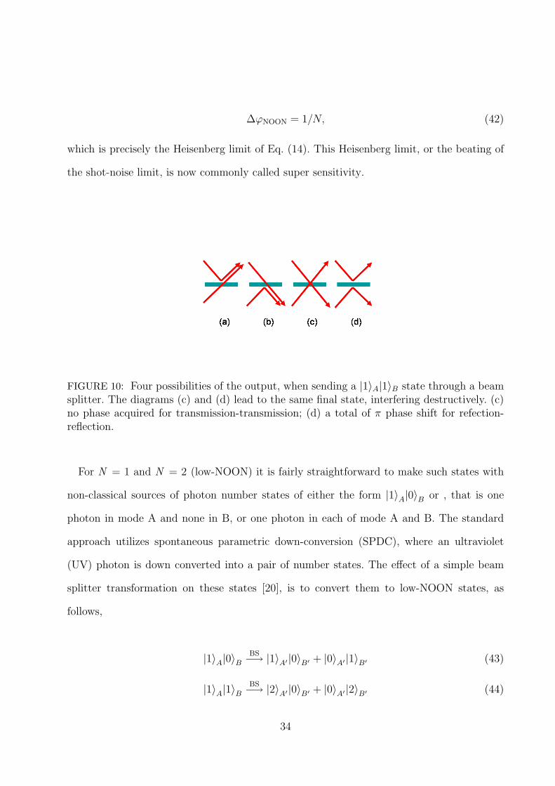
FIGURE 10: Four possibilities of the output, when sending a |1〉A|1〉B state through a beamsplitter. The diagrams (c) and (d) lead to the same final state, interfering destructively. (c)no phase acquired for transmission-transmission; (d) a total of π phase shift for refection-reflection.
For N = 1 and N = 2 (low-NOON) it is fairly straightforward to make such states with
non-classical sources of photon number states of either the form |1〉A|0〉B or , that is one
photon in mode A and none in B, or one photon in each of mode A and B. The standard
approach utilizes spontaneous parametric down-conversion (SPDC), where an ultraviolet
(UV) photon is down converted into a pair of number states. The effect of a simple beam
splitter transformation on these states [20], is to convert them to low-NOON states, as
follows,
|1〉A|0〉BBS−→ |1〉A′|0〉B′ + |0〉A′|1〉B′ (43)
|1〉A|1〉BBS−→ |2〉A′|0〉B′ + |0〉A′|2〉B′ (44)
34
where Eq. (43) shows that a single photon cannot be split in two, and Eq. (44) is illustrative
of the more subtle Hong-Ou-Mandel effect — if two single photons are incident on a 50-50
beam splitter they will stick and both photons will go one way or both will go the other way,
but you never get one photon out each port [62].
As depicted in Fig.10, it is the probability amplitude for the transition |1〉A|1〉BBS−→
|1〉A′|1〉B′ that completely cancels out due to destructive interference. On the other hand, the
probability amplitude for the transition indicated by Eq. (44) adds up, due to constructive
interference. So it is relatively easy, once you have a source of single photons, to create
low-NOON states. The current ongoing challenge is to find practical ways of making high
numbered NOON states.
Now that we have reviewed the basic properties of NOON states, we are prepared to
examine what happens to them when they encounter real-world losses.
3.2 Environmental Decoherence
A realistic model of propagation loss is essential in determining the usefulness of entangled
states for real-world applications. Studies have recently appeared that deal with limits to
phase measurement precision specifically for N00N states that experience loss [63, 64]. These
studies conclude that loss in either arm diminishes phase sensitivity rapidly, and under
some limits sensor performance is worse than with coherent light. This loss issue presents a
potential problem for any type of sensor application using N00N states.
In this section we address how environmental interaction brings about decoherence for a
more generalized Fock state with photons in both modes, and we have discovered a class of
states that improve drastically on the performance of N00N states when loss is present. We
find with these new states that while minimum sensitivity is slightly decreased, robustness
against decoherence is greatly increased.
For practical purposes phase sensitivity is typically obtained by the linear error propa-
gation method, (see however Ref. [65]), where O represents the operator for the detection
35
scheme being used,
δφ =∆O∣∣∣ ∂〈O〉/∂φ
∣∣∣, (45)
and ∆ON =
√〈O2〉 − 〈O〉2. Eq. (45), for a N00N state with no loss, and a detection operator
AN = |0, N〉 〈N, 0|+ |N, 0〉 〈0, N | , (46)
which can be implemented with coincidence measurements [66], reduces to the Heisenberg
limit, δφ = 1/N , which is a√
N improvement over the shot-noise limit.
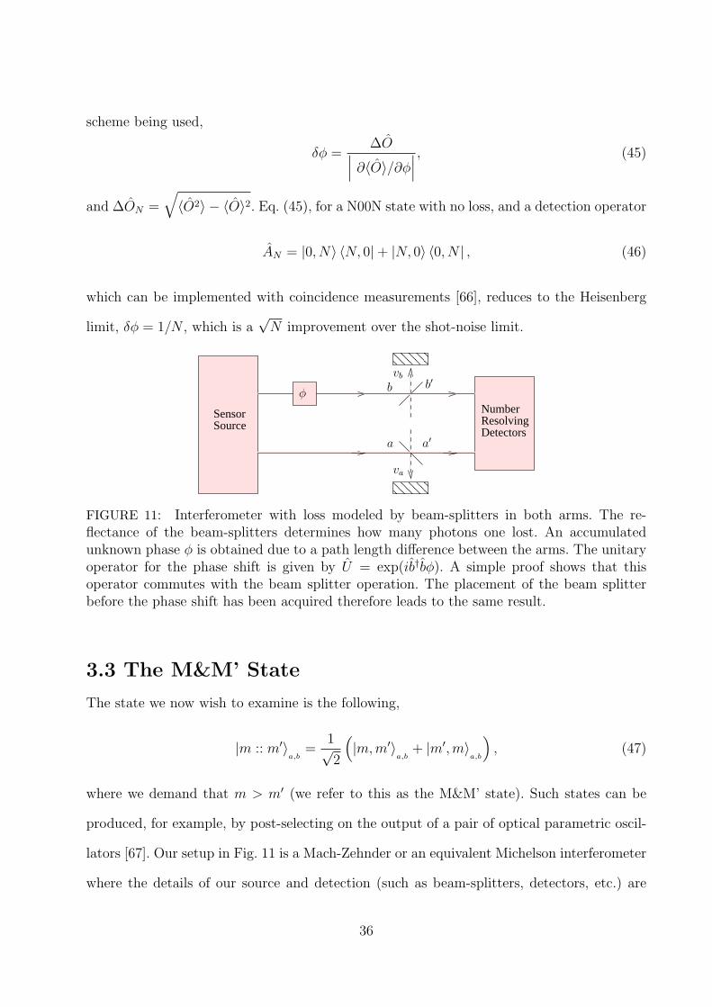
SensorSource
NumberResolvingDetectors
b′
vb
a′
b
va
a
φ
FIGURE 11: Interferometer with loss modeled by beam-splitters in both arms. The re-flectance of the beam-splitters determines how many photons one lost. An accumulatedunknown phase φ is obtained due to a path length difference between the arms. The unitaryoperator for the phase shift is given by U = exp(ib†bφ). A simple proof shows that thisoperator commutes with the beam splitter operation. The placement of the beam splitterbefore the phase shift has been acquired therefore leads to the same result.
3.3 The M&M’ State
The state we now wish to examine is the following,
|m :: m′〉a,b
=1√2
(|m,m′〉
a,b+ |m′,m〉
a,b
), (47)
where we demand that m > m′ (we refer to this as the M&M’ state). Such states can be
produced, for example, by post-selecting on the output of a pair of optical parametric oscil-
lators [67]. Our setup in Fig. 11 is a Mach-Zehnder or an equivalent Michelson interferometer
where the details of our source and detection (such as beam-splitters, detectors, etc.) are
36
contained in their respective boxes. Here we are concerned primarily with how the state
evolves with respect to loss, which is typically modeled by additional beam-splitters coupled
to the environment [68].
Similar to the approach of Ref. [64], we model loss in the interferometer with fictitious
beam-splitters, but in our case these are added to both arms of the interferometer. However
we assume unit detection efficiency for the detectors. We develop the photon statistics as a
function of beam-splitter transmittance as well as derive a reduced density matrix, which
characterizes the propagation losses inside of the interferometer. Loss is represented by pho-
tons being reflected into the environment [69]. The beam-splitter transforms the modes
according to [20],
a′ = taa + r∗aav ,
b′ = tbb + r∗b bv , (48)
where tu =√
Tu exp(iϕu) and ru =√
Ru exp(iψu), u = a, b, are the complex transmission
and reflectance coefficients, for mode a and b, respectively. The input M&M’ state |m :: m′〉acquires an unknown phase shift φ and the beam splitter transformations are applied,
|ψ〉 =1√
2m!m′!
m∑
k=0
m′∑
l=0
m
k
m′
l
[(m− k)!k!(m′ − l)!l!]1/2
× (t∗m−ka r∗ka (t∗be
iφ)m′−lr∗lb |m− k, m′ − l〉a′,b′|k, l〉va,vb
+ t∗m′−l
a r∗la (t∗beiφ)m−kr∗kb |m′ − l, m− k〉a,b′|l, k〉va,vb
). (49)
37
We then trace over the environmental modes, to model the photons lost, and we obtain
the reduced density matrix ρa′,b′ = Trva,vb[|ψ〉〈ψ|], which leads to
ρa′,b′ =m∑
k=0
m′∑
l,l′=0
|ak,l|2|m− k, m′ − l〉〈m− k, m′ − l|
+ |bk,l|2|m′ − l, m− k〉〈m′ − l,m− k|
+ a∗l,l′bl′,l|m′ − l, m− l′〉〈m− l,m′ − l′|
+ al′,lb∗l,l′|m− l′,m′ − l〉〈m′ − l′,m− l| . (50)
Here the ak,l and bk,l coefficients are defined as
|ak,l|2 ≡ γ2k,lT
m−ka Rk
aTm′−lb Rl
b ,
|bk,l|2 ≡ γ2k,lT
m′−la Rl
aTm−kb Rk
b ,
a∗l,l′bl′,l ≡ γl,l′γl′,lTm+m′−2l
2a Rl
aTm+m′−2l′
2b Rl′
b e−i(m−m′)(φ+ϕb−ϕa) ,
al′,lb∗l,l′ ≡ γl′,lγl,l′T
m+m′−2l′2
a Rl′aT
m+m′−2l2
b Rlbe
i(m−m′)(φ+ϕb−ϕa), (51)
and
γk,l ≡ 1√2m!m′!
m
k
m′
l
[(m− k)!k! (m′ − l)!l!]
1/2. (52)
Without loss of generality we can set the transmission phases of the two beam splitters
ϕa = ϕb = 0.
The reduced density matrix in Eq. (50) appears as an incoherent mixture plus interference
terms, which survive with loss in either mode up to the limit of m′. The surviving interference
terms all carry amplified phase information in the quantity (m −m′)φ. Thus the best-case
minimum phase sensitivity, under no loss, is reduced from the Heisenberg limit, δφN00N =
1/N , to δφm,m′ = 1/(m −m′). Although this sensitivity is less than what N00N states are
capable of achieving (in the absence of loss), the fact that many more interference terms
survive than with N00N states suggests that these states are more robust against photon
loss. For comparison, we can easily see the reduced density matrix for a NOON state by
38
setting m′ = 0 in Eq.50,
ρN00N =m∑
k=0
|ak,0|2|N − k, 0〉〈N − k, 0|
+ |bk,0|2|0, N − k〉〈0, N − k|
+ a∗0,0b0,0|0, N〉〈N, 0|
+ a0,0b∗0,0|N, 0〉〈0, N |. (53)
We see in Eq. (53) why NOON states are so fragile; the only off-diagonal terms in the reduced
density matrix that survive are for the case in which there is absolutely no photon loss. If a
NOON state loses a single photon anywhere in the interferometer the collapsed state provides
zero phase information.
3.4 Operator Selection and Visibility
To maximize phase information we choose a detection operator of the form
A =m′∑
r,s=0
|m′ − r,m− s〉〈m− r,m′ − s|
+|m− r,m′ − s〉〈m′ − r,m− s| , (54)
which we will show is theoretically optimal. This operator is a more general summation over
all possible cases up to m′ photons in either arm than the AN operator (traditionally used
for N00N states [9]). Using the reduced density matrix we derived with the NOON state in
Eq.53 we obtain for the expectation value of AN
〈AN〉 = Tr[AN ρa′,b′ ] = 2Re(a∗0,0b0,0
)
= (TaTb)N2 cos(Nφ) . (55)
39
The expectation value of the operator A given in Eq. (54) for the M&M’ state shows the
benefit of having many more interference terms compared to the N00N state
〈A〉 = Tr[Aρa′,b′ ] = 2Re
(m′∑
l,l′=0
a∗l,l′bl′,l
)
= 2m′∑
l,l′=0
∣∣a∗l,l′bl′,l∣∣ cos[(m−m′)φ] . (56)
To prove that we have chosen the best possible theoretical operator we use the work of
Mandel, who showed the visibility of any pure or attenuated mixed state in an interferometer
may be expressed as a function of the off-diagonal terms in the reduced density matrix from
Eq. (50) [70],
Vf = 2 |ρ1,2| = 2
∣∣∣∣∣m′∑
l,l′=0
a∗l,l′bl′,l
∣∣∣∣∣ = 2m′∑
l,l′=0
∣∣a∗l,l′bl′,l∣∣ , (57)
where we call Vf the fundamental visibility and ρ1,2 is taken from one of the off-diagonal
terms in the density matrix in Eq. (50). Our task now is to choose an operator capable of
sensing at the fundamental visibility limit. Any detection operator O exhibiting an amplitude
smaller than Vf , i.e., Vf ≥ 〈O〉Φ=0, is not using all available off-diagonal terms, and thus
not optimal. From Eqs. (56,57) we see that the expectation value of A may be written as
〈A〉 = Vf cos[(m−m′)φ]. We call the visibility of a particular detection scheme the detection
visibility, Vdet = 〈O〉φ=0. We see that the AN operator, and its more general form A in
Eq. (54), are both optimal for N00N and M&M’ states, respectively, and give a detection
visibility equivalent to the fundamental visibility. The fundamental visibility for a N00N
state is simply Vf = (TaTb)N/2, which is just the probability the N00N state arrives at the
detector with no loss.
3.5 Increased Robustness of the M&M’ State to
Photon Loss
The M&M’ states, with m − m′ = N , are capable of producing the same resolution as a
N photon N00N state, but at the cost of requiring m′ more photons to do so, and thus
40
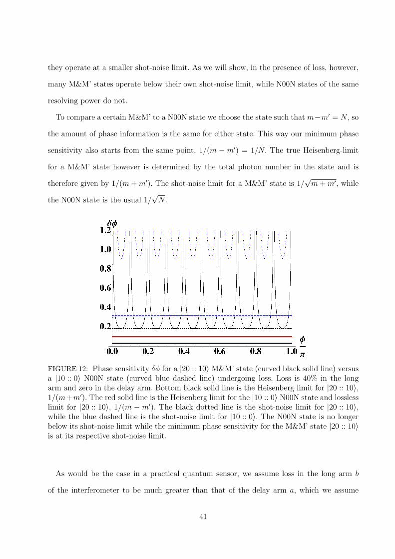
they operate at a smaller shot-noise limit. As we will show, in the presence of loss, however,
many M&M’ states operate below their own shot-noise limit, while N00N states of the same
resolving power do not.
To compare a certain M&M’ to a N00N state we choose the state such that m−m′ = N , so
the amount of phase information is the same for either state. This way our minimum phase
sensitivity also starts from the same point, 1/(m − m′) = 1/N. The true Heisenberg-limit
for a M&M’ state however is determined by the total photon number in the state and is
therefore given by 1/(m + m′). The shot-noise limit for a M&M’ state is 1/√
m + m′, while
the N00N state is the usual 1/√
N .
FIGURE 12: Phase sensitivity δφ for a |20 :: 10〉 M&M’ state (curved black solid line) versusa |10 :: 0〉 N00N state (curved blue dashed line) undergoing loss. Loss is 40% in the longarm and zero in the delay arm. Bottom black solid line is the Heisenberg limit for |20 :: 10〉,1/(m+m′). The red solid line is the Heisenberg limit for the |10 :: 0〉 N00N state and losslesslimit for |20 :: 10〉, 1/(m − m′). The black dotted line is the shot-noise limit for |20 :: 10〉,while the blue dashed line is the shot-noise limit for |10 :: 0〉. The N00N state is no longerbelow its shot-noise limit while the minimum phase sensitivity for the M&M’ state |20 :: 10〉is at its respective shot-noise limit.
As would be the case in a practical quantum sensor, we assume loss in the long arm b
of the interferometer to be much greater than that of the delay arm a, which we assume
41
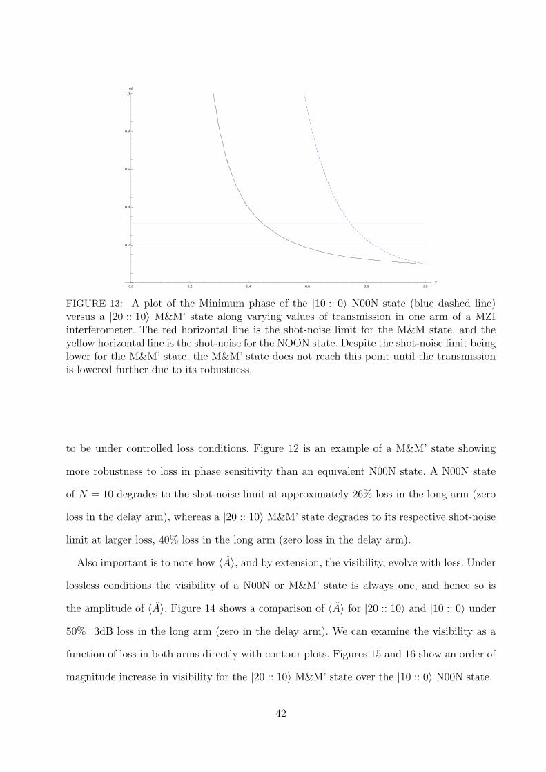
0.0 0.2 0.4 0.6 0.8 1.0T
0.2
0.4
0.6
0.8
1.0
∆Φ
FIGURE 13: A plot of the Minimum phase of the |10 :: 0〉 N00N state (blue dashed line)versus a |20 :: 10〉 M&M’ state along varying values of transmission in one arm of a MZIinterferometer. The red horizontal line is the shot-noise limit for the M&M state, and theyellow horizontal line is the shot-noise for the NOON state. Despite the shot-noise limit beinglower for the M&M’ state, the M&M’ state does not reach this point until the transmissionis lowered further due to its robustness.
to be under controlled loss conditions. Figure 12 is an example of a M&M’ state showing
more robustness to loss in phase sensitivity than an equivalent N00N state. A N00N state
of N = 10 degrades to the shot-noise limit at approximately 26% loss in the long arm (zero
loss in the delay arm), whereas a |20 :: 10〉 M&M’ state degrades to its respective shot-noise
limit at larger loss, 40% loss in the long arm (zero loss in the delay arm).
Also important is to note how 〈A〉, and by extension, the visibility, evolve with loss. Under
lossless conditions the visibility of a N00N or M&M’ state is always one, and hence so is
the amplitude of 〈A〉. Figure 14 shows a comparison of 〈A〉 for |20 :: 10〉 and |10 :: 0〉 under
50%=3dB loss in the long arm (zero in the delay arm). We can examine the visibility as a
function of loss in both arms directly with contour plots. Figures 15 and 16 show an order of
magnitude increase in visibility for the |20 :: 10〉 M&M’ state over the |10 :: 0〉 N00N state.
42
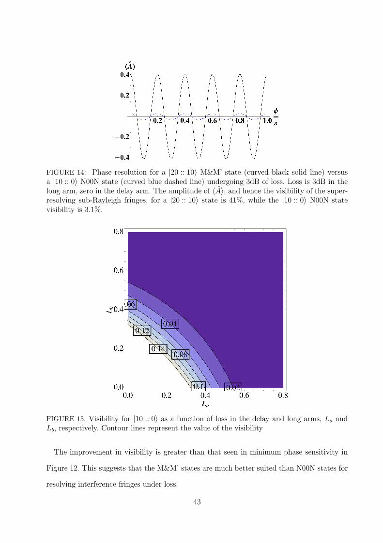
FIGURE 14: Phase resolution for a |20 :: 10〉 M&M’ state (curved black solid line) versusa |10 :: 0〉 N00N state (curved blue dashed line) undergoing 3dB of loss. Loss is 3dB in thelong arm, zero in the delay arm. The amplitude of 〈A〉, and hence the visibility of the super-resolving sub-Rayleigh fringes, for a |20 :: 10〉 state is 41%, while the |10 :: 0〉 N00N statevisibility is 3.1%.
FIGURE 15: Visibility for |10 :: 0〉 as a function of loss in the delay and long arms, La andLb, respectively. Contour lines represent the value of the visibility
The improvement in visibility is greater than that seen in minimum phase sensitivity in
Figure 12. This suggests that the M&M’ states are much better suited than N00N states for
resolving interference fringes under loss.
43
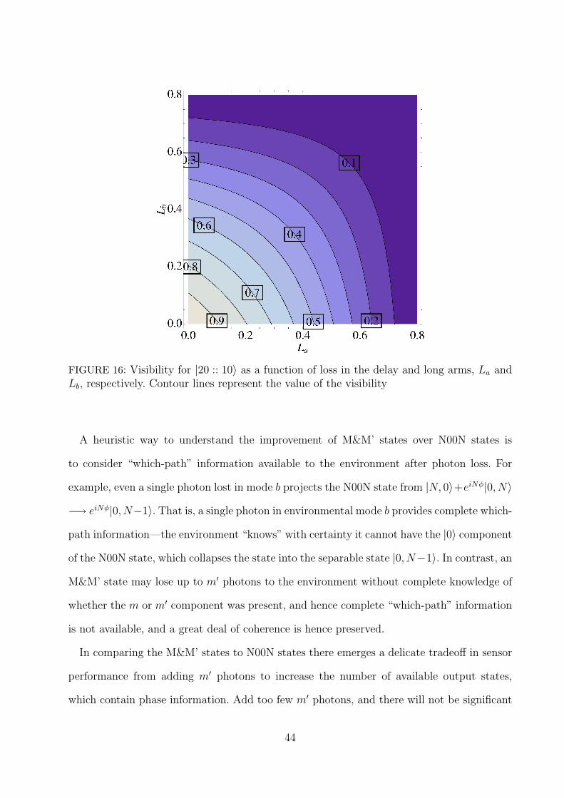
FIGURE 16: Visibility for |20 :: 10〉 as a function of loss in the delay and long arms, La andLb, respectively. Contour lines represent the value of the visibility
A heuristic way to understand the improvement of M&M’ states over N00N states is
to consider “which-path” information available to the environment after photon loss. For
example, even a single photon lost in mode b projects the N00N state from |N, 0〉+eiNφ|0, N〉−→ eiNφ|0, N−1〉. That is, a single photon in environmental mode b provides complete which-
path information—the environment “knows” with certainty it cannot have the |0〉 component
of the N00N state, which collapses the state into the separable state |0, N−1〉. In contrast, an
M&M’ state may lose up to m′ photons to the environment without complete knowledge of
whether the m or m′ component was present, and hence complete “which-path” information
is not available, and a great deal of coherence is hence preserved.
In comparing the M&M’ states to N00N states there emerges a delicate tradeoff in sensor
performance from adding m′ photons to increase the number of available output states,
which contain phase information. Add too few m′ photons, and there will not be significant
44
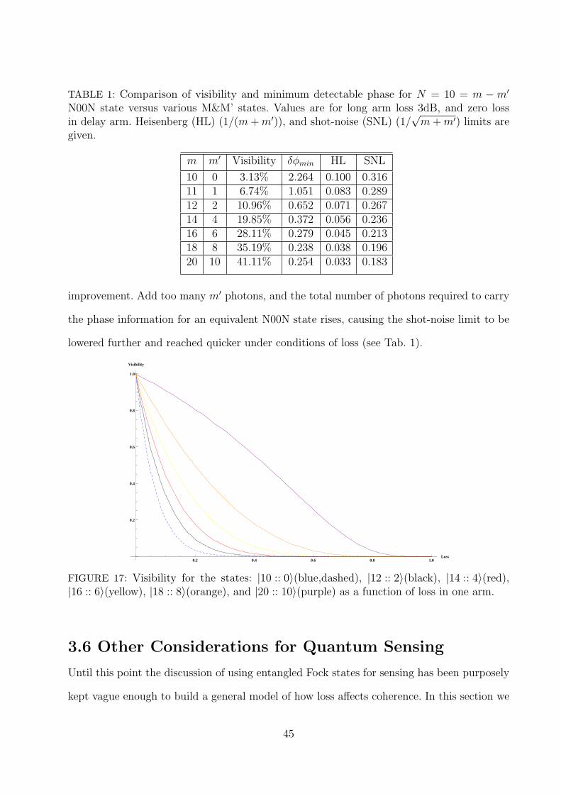
TABLE 1: Comparison of visibility and minimum detectable phase for N = 10 = m − m′
N00N state versus various M&M’ states. Values are for long arm loss 3dB, and zero lossin delay arm. Heisenberg (HL) (1/(m + m′)), and shot-noise (SNL) (1/
√m + m′) limits are
given.
m m′ Visibility δφmin HL SNL
10 0 3.13% 2.264 0.100 0.31611 1 6.74% 1.051 0.083 0.28912 2 10.96% 0.652 0.071 0.26714 4 19.85% 0.372 0.056 0.23616 6 28.11% 0.279 0.045 0.21318 8 35.19% 0.238 0.038 0.19620 10 41.11% 0.254 0.033 0.183
improvement. Add too many m′ photons, and the total number of photons required to carry
the phase information for an equivalent N00N state rises, causing the shot-noise limit to be
lowered further and reached quicker under conditions of loss (see Tab. 1).
0.2 0.4 0.6 0.8 1.0Loss
0.2
0.4
0.6
0.8
1.0
Visibility
FIGURE 17: Visibility for the states: |10 :: 0〉(blue,dashed), |12 :: 2〉(black), |14 :: 4〉(red),|16 :: 6〉(yellow), |18 :: 8〉(orange), and |20 :: 10〉(purple) as a function of loss in one arm.
3.6 Other Considerations for Quantum Sensing
Until this point the discussion of using entangled Fock states for sensing has been purposely
kept vague enough to build a general model of how loss affects coherence. In this section we
45
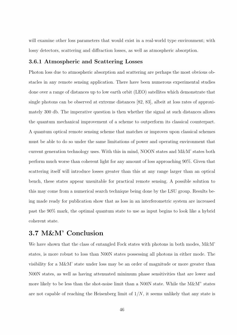
will examine other loss parameters that would exist in a real-world type environment; with
lossy detectors, scattering and diffraction losses, as well as atmospheric absorption.
3.6.1 Atmospheric and Scattering Losses
Photon loss due to atmospheric absorption and scattering are perhaps the most obvious ob-
stacles in any remote sensing application. There have been numerous experimental studies
done over a range of distances up to low earth orbit (LEO) satellites which demonstrate that
single photons can be observed at extreme distances [82, 83], albeit at loss rates of approxi-
mately 300 db. The imperative question is then whether the signal at such distances allows
the quantum mechanical improvement of a scheme to outperform its classical counterpart.
A quantum optical remote sensing scheme that matches or improves upon classical schemes
must be able to do so under the same limitations of power and operating environment that
current generation technology uses. With this in mind, NOON states and M&M’ states both
perform much worse than coherent light for any amount of loss approaching 90%. Given that
scattering itself will introduce losses greater than this at any range larger than an optical
bench, these states appear unsuitable for practical remote sensing. A possible solution to
this may come from a numerical search technique being done by the LSU group. Results be-
ing made ready for publication show that as loss in an interferometric system are increased
past the 90% mark, the optimal quantum state to use as input begins to look like a hybrid
coherent state.
3.7 M&M’ Conclusion
We have shown that the class of entangled Fock states with photons in both modes, M&M’
states, is more robust to loss than N00N states possessing all photons in either mode. The
visibility for a M&M’ state under loss may be an order of magnitude or more greater than
N00N states, as well as having attenuated minimum phase sensitivities that are lower and
more likely to be less than the shot-noise limit than a N00N state. While the M&M” states
are not capable of reaching the Heisenberg limit of 1/N , it seems unlikely that any state is
46
capable of reaching this precision in the limit of practical sensing with appreciable photon
loss. While M&M’ states are more robust, they do appear to have loss-induced limitations
as well. For many M&M’ states visibility drops to approximately 10% around the 70% loss
level in one arm, assuming perfect transmission in the other.
Other issues that need consideration are how to produce M&M’ states and how to optimally
detect them. As of yet there is no efficient, on demand, Fock number state generator. However
the output from a optical parametric amplifier (OPA) is essentially a summation of many
M&M’ states as well as several N00N states. While we know what the optimal operators look
like mathematically, it is also currently unknown how to produce these in the lab. There is
ongoing work analyzing the sensing capabilities for the entire output state of an OPA, as
well as schemes for generating M&M’ states from an OPA output with post-selection. There
have also been preliminary results which indicate that M&M’ photons may have properties
which make them better suited for material absorption [86].
As of this writing there are preliminary results from Professor Kwiat’s group at Illinois
Urbana-Champaign that M&M states have been made experimentally, and may in fact be
easier to produce than NOON states.
47
4 Improvement of Fabry-PerotInterferometers with Entangled State Input
In this chapter we present a model for quantum Mie scattering in one dimension, and show
that quantum states of light, such as Fock states, exhibit the same transmission functions
as coherent states for an ordinary intensity measurement. However, if a number-resolving
measurement is carried out instead, we observe narrower transmission functions than for the
classical case. We discuss applications of this effect for high-precision length measurements
in interferometry. The findings of this chapter were published in Proc. SPIE, Vol. 7225,
72250Q (2009).
Quantum states of light play an important role for applications such as metrology, imaging,
and sensing. We have just scratched the surface of this new field of quantum enhanced
technologies, and progress has been reported for many metrology schemes. However, for real
world applications, diffraction, scattering, and absorption of quantum states of light need to
be taken into account. Many quantum enhanced metrology schemes perform poorly when a
considerable amount of loss is present [63, 64, 81]. However, quantum states that are more
resilient to loss have recently been found [87]. These states still outperform classical light
sources under a moderate 3 dB of loss. So stand-off applications with limited range, such as
a LADAR (Light RADAR) with nonclassical light, seems to be within reach.
An important problem in conventional radar ranging and imaging applications is Mie scat-
tering. To determine the correct radar cross section of a spherical object, which is about the
size of the wavelength, we must use Mie scattering theory. The scattering of plane waves
off homogeneous spherical objects is very well described by the Mie scattering solution of
the Maxwell equations [88]. But what happens if we replace the classical incoming elec-
tromagnetic wave with a nonclassical state of light? Does the nonclassical light obey the
same scattering solution? To answer this question we need to develop a fully quantized Mie
scattering theory.
48
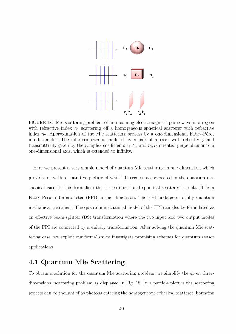
FIGURE 18: Mie scattering problem of an incoming electromagnetic plane wave in a regionwith refractive index n1 scattering off a homogeneous spherical scatterer with refractiveindex n2. Approximation of the Mie scattering process by a one-dimensional Fabry-Perotinterferometer. The interferometer is modeled by a pair of mirrors with reflectivity andtransmittivity given by the complex coefficients r1, t1, and r2, t2 oriented perpendicular to aone-dimensional axis, which is extended to infinity.
Here we present a very simple model of quantum Mie scattering in one dimension, which
provides us with an intuitive picture of which differences are expected in the quantum me-
chanical case. In this formalism the three-dimensional spherical scatterer is replaced by a
Fabry-Perot interferometer (FPI) in one dimension. The FPI undergoes a fully quantum
mechanical treatment. The quantum mechanical model of the FPI can also be formulated as
an effective beam-splitter (BS) transformation where the two input and two output modes
of the FPI are connected by a unitary transformation. After solving the quantum Mie scat-
tering case, we exploit our formalism to investigate promising schemes for quantum sensor
applications.
4.1 Quantum Mie Scattering
To obtain a solution for the quantum Mie scattering problem, we simplify the given three-
dimensional scattering problem as displayed in Fig. 18. In a particle picture the scattering
process can be thought of as photons entering the homogeneous spherical scatterer, bouncing
49
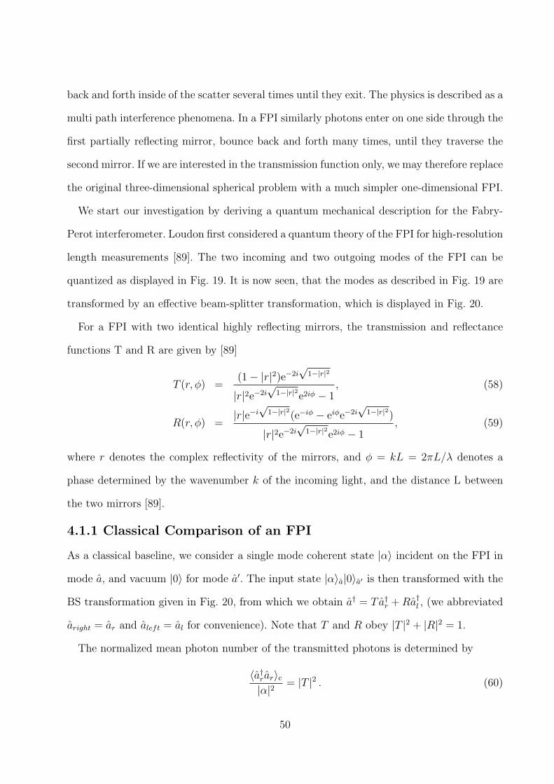
back and forth inside of the scatter several times until they exit. The physics is described as a
multi path interference phenomena. In a FPI similarly photons enter on one side through the
first partially reflecting mirror, bounce back and forth many times, until they traverse the
second mirror. If we are interested in the transmission function only, we may therefore replace
the original three-dimensional spherical problem with a much simpler one-dimensional FPI.
We start our investigation by deriving a quantum mechanical description for the Fabry-
Perot interferometer. Loudon first considered a quantum theory of the FPI for high-resolution
length measurements [89]. The two incoming and two outgoing modes of the FPI can be
quantized as displayed in Fig. 19. It is now seen, that the modes as described in Fig. 19 are
transformed by an effective beam-splitter transformation, which is displayed in Fig. 20.
For a FPI with two identical highly reflecting mirrors, the transmission and reflectance
functions T and R are given by [89]
T (r, φ) =(1− |r|2)e−2i
√1−|r|2
|r|2e−2i√
1−|r|2e2iφ − 1, (58)
R(r, φ) =|r|e−i
√1−|r|2(e−iφ − eiφe−2i
√1−|r|2)
|r|2e−2i√
1−|r|2e2iφ − 1, (59)
where r denotes the complex reflectivity of the mirrors, and φ = kL = 2πL/λ denotes a
phase determined by the wavenumber k of the incoming light, and the distance L between
the two mirrors [89].
4.1.1 Classical Comparison of an FPI
As a classical baseline, we consider a single mode coherent state |α〉 incident on the FPI in
mode a, and vacuum |0〉 for mode a′. The input state |α〉a|0〉a′ is then transformed with the
BS transformation given in Fig. 20, from which we obtain a† = T a†r + Ra†l , (we abbreviated
aright = ar and aleft = al for convenience). Note that T and R obey |T |2 + |R|2 = 1.
The normalized mean photon number of the transmitted photons is determined by
〈a†rar〉c|α|2 = |T |2 . (60)
50
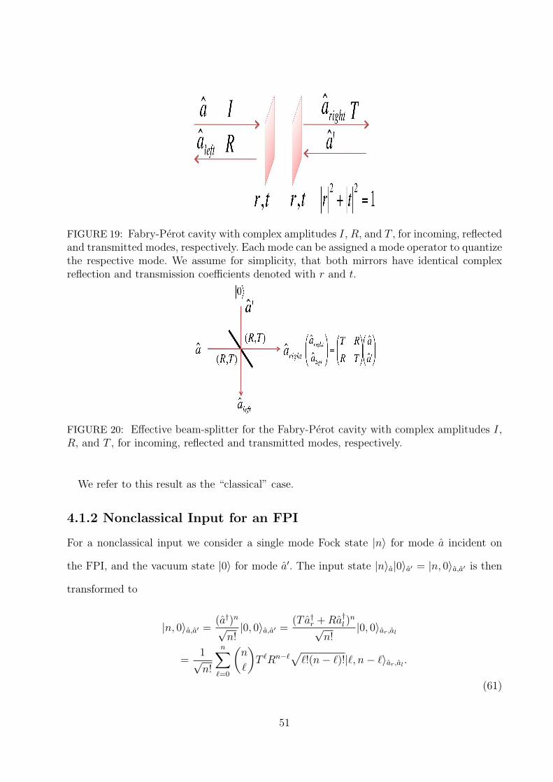
FIGURE 19: Fabry-Perot cavity with complex amplitudes I, R, and T , for incoming, reflectedand transmitted modes, respectively. Each mode can be assigned a mode operator to quantizethe respective mode. We assume for simplicity, that both mirrors have identical complexreflection and transmission coefficients denoted with r and t.
FIGURE 20: Effective beam-splitter for the Fabry-Perot cavity with complex amplitudes I,R, and T , for incoming, reflected and transmitted modes, respectively.
We refer to this result as the “classical” case.
4.1.2 Nonclassical Input for an FPI
For a nonclassical input we consider a single mode Fock state |n〉 for mode a incident on
the FPI, and the vacuum state |0〉 for mode a′. The input state |n〉a|0〉a′ = |n, 0〉a,a′ is then
transformed to
|n, 0〉a,a′ =(a†)n
√n!|0, 0〉a,a′ =
(T a†r + Ra†l )n
√n!
|0, 0〉ar,al
=1√n!
n∑
`=0
(n
`
)T `Rn−`
√`!(n− `)!|`, n− `〉ar,al
.
(61)
51
The normalized mean photon counts at the output of the FPI are obtained from the expec-
tation value
〈a†rar〉Fn
= |T |2 . (62)
We obtain the same transmission function as in the classical case. However, if we make a
number resolving measurement described by the detection operator C = |n〉〈n| for mode ar,
we obtain a different behavior given by
〈C〉 = Tr(CρF
)= |T |2n . (63)
Where ρF is the reduced density matrix for the Fock state in mode ar. It turns out that the
transmission function becomes narrower as a function of the photon number n (see Fig. 21).
It still remains to be checked whether replacing an ordinary mean intensity measurement
with the number resolving detection operator C always leads to a narrowing of the trans-
mission functions. Therefore we consider the coherent state |α, 0〉a,a′ , and apply a n-photon
detection C = |n〉〈n| for mode ar, which leads to the expression
〈C〉 = Tr(Cρc
)
= e−|α|2∞∑
k=n
|α|2k
n!(k − n)!|T |2n|R|2(k−n). (64)
Where ρc is the reduced density matrix for the coherent state in mode ar. We display this
result, and all previous results in Fig. 21 for comparison.
The coherent state input, together with a number resolving measurement, leads to a broad-
ening of the transmission function with a low amplitude of the transmission maxima com-
pared to a mean intensity measurement. On the other hand we observe that the transmission
function for the two-photon Fock state and a two-photon detection clearly becomes narrower
than in the classical case.
So far, our simple model for quantum Mie scattering provides us with the answer of
what differences between classical and nonclassical input states with particular detection
52
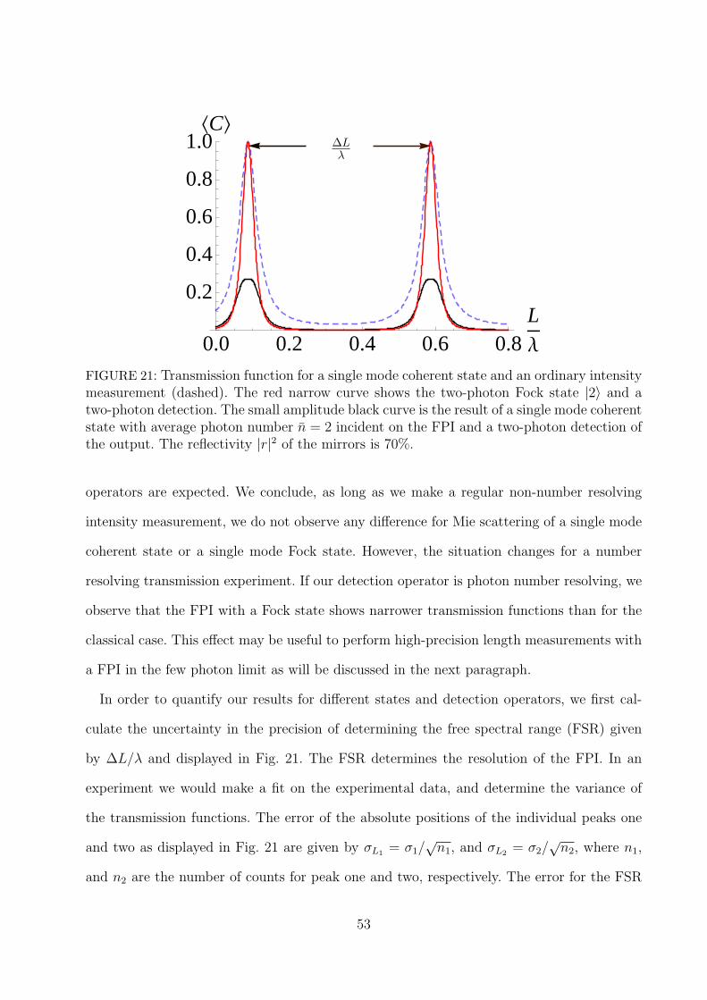
0.0 0.2 0.4 0.6 0.8LΛ
0.2
0.4
0.6
0.8
1.0XC\
∆L
λ
FIGURE 21: Transmission function for a single mode coherent state and an ordinary intensitymeasurement (dashed). The red narrow curve shows the two-photon Fock state |2〉 and atwo-photon detection. The small amplitude black curve is the result of a single mode coherentstate with average photon number n = 2 incident on the FPI and a two-photon detection ofthe output. The reflectivity |r|2 of the mirrors is 70%.
operators are expected. We conclude, as long as we make a regular non-number resolving
intensity measurement, we do not observe any difference for Mie scattering of a single mode
coherent state or a single mode Fock state. However, the situation changes for a number
resolving transmission experiment. If our detection operator is photon number resolving, we
observe that the FPI with a Fock state shows narrower transmission functions than for the
classical case. This effect may be useful to perform high-precision length measurements with
a FPI in the few photon limit as will be discussed in the next paragraph.
In order to quantify our results for different states and detection operators, we first cal-
culate the uncertainty in the precision of determining the free spectral range (FSR) given
by ∆L/λ and displayed in Fig. 21. The FSR determines the resolution of the FPI. In an
experiment we would make a fit on the experimental data, and determine the variance of
the transmission functions. The error of the absolute positions of the individual peaks one
and two as displayed in Fig. 21 are given by σL1 = σ1/√
n1, and σL2 = σ2/√
n2, where n1,
and n2 are the number of counts for peak one and two, respectively. The error for the FSR
53
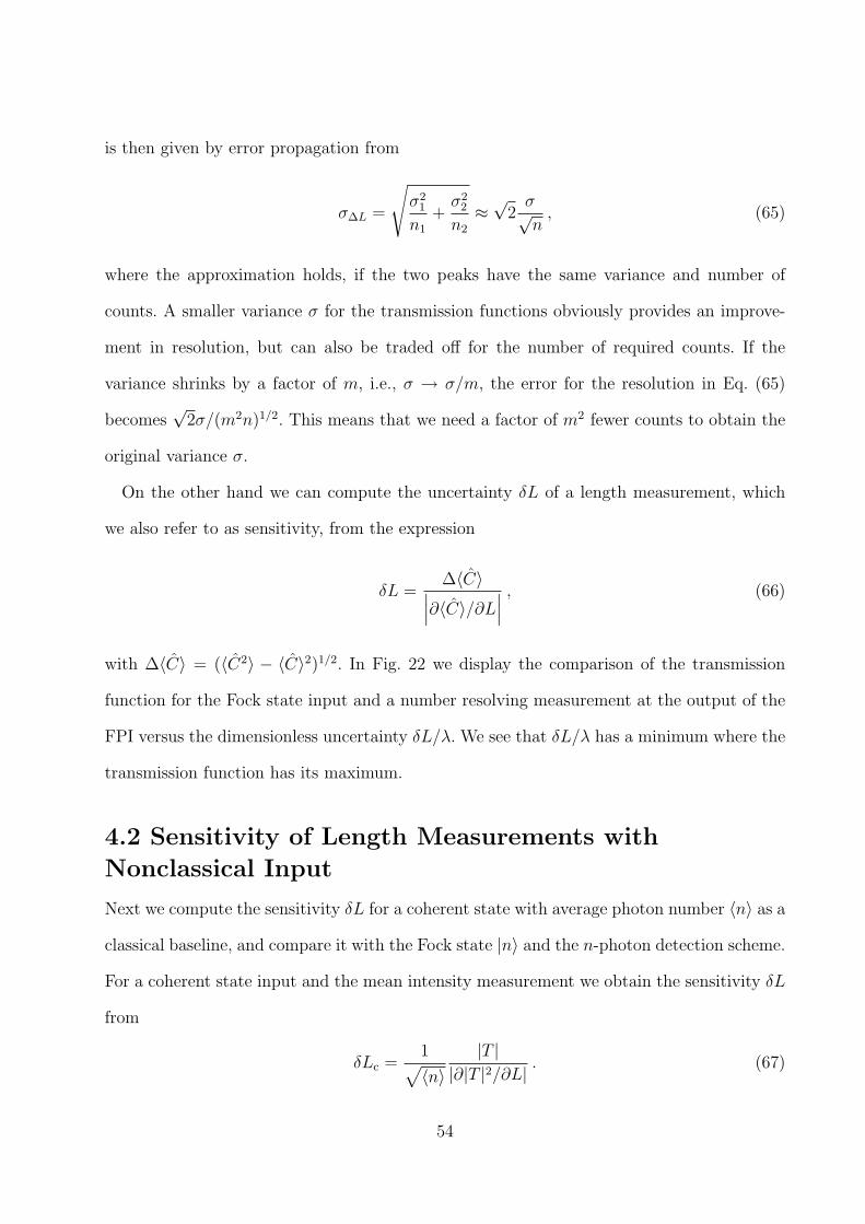
is then given by error propagation from
σ∆L =
√σ2
1
n1
+σ2
2
n2
≈√
2σ√n
, (65)
where the approximation holds, if the two peaks have the same variance and number of
counts. A smaller variance σ for the transmission functions obviously provides an improve-
ment in resolution, but can also be traded off for the number of required counts. If the
variance shrinks by a factor of m, i.e., σ → σ/m, the error for the resolution in Eq. (65)
becomes√
2σ/(m2n)1/2. This means that we need a factor of m2 fewer counts to obtain the
original variance σ.
On the other hand we can compute the uncertainty δL of a length measurement, which
we also refer to as sensitivity, from the expression
δL =∆〈C〉∣∣∣∂〈C〉/∂L
∣∣∣, (66)
with ∆〈C〉 = (〈C2〉 − 〈C〉2)1/2. In Fig. 22 we display the comparison of the transmission
function for the Fock state input and a number resolving measurement at the output of the
FPI versus the dimensionless uncertainty δL/λ. We see that δL/λ has a minimum where the
transmission function has its maximum.
4.2 Sensitivity of Length Measurements with
Nonclassical Input
Next we compute the sensitivity δL for a coherent state with average photon number 〈n〉 as a
classical baseline, and compare it with the Fock state |n〉 and the n-photon detection scheme.
For a coherent state input and the mean intensity measurement we obtain the sensitivity δL
from
δLc =1√〈n〉
|T ||∂|T |2/∂L| . (67)
54
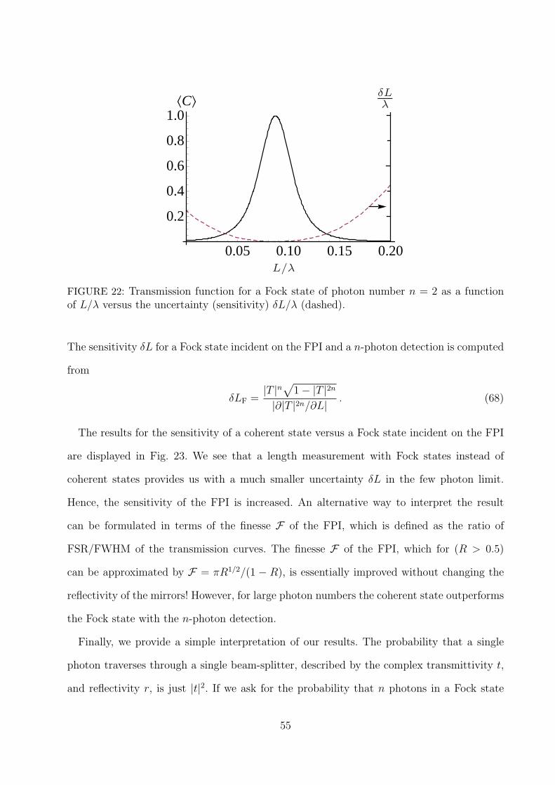
0.05 0.10 0.15 0.20
0.2
0.4
0.6
0.8
1.0XC\
L/λ
δLλ
FIGURE 22: Transmission function for a Fock state of photon number n = 2 as a functionof L/λ versus the uncertainty (sensitivity) δL/λ (dashed).
The sensitivity δL for a Fock state incident on the FPI and a n-photon detection is computed
from
δLF =|T |n
√1− |T |2n
|∂|T |2n/∂L| . (68)
The results for the sensitivity of a coherent state versus a Fock state incident on the FPI
are displayed in Fig. 23. We see that a length measurement with Fock states instead of
coherent states provides us with a much smaller uncertainty δL in the few photon limit.
Hence, the sensitivity of the FPI is increased. An alternative way to interpret the result
can be formulated in terms of the finesse F of the FPI, which is defined as the ratio of
FSR/FWHM of the transmission curves. The finesse F of the FPI, which for (R > 0.5)
can be approximated by F = πR1/2/(1 − R), is essentially improved without changing the
reflectivity of the mirrors! However, for large photon numbers the coherent state outperforms
the Fock state with the n-photon detection.
Finally, we provide a simple interpretation of our results. The probability that a single
photon traverses through a single beam-splitter, described by the complex transmittivity t,
and reflectivity r, is just |t|2. If we ask for the probability that n photons in a Fock state
55
200 400 600 800Xn\0.000
0.002
0.004
0.006
0.008
0.010
∆LΛ
FIGURE 23: Comparison of the sensitivity δL/λ for a coherent state (solid line) versus a Fockstate with n-photon resolving measurement as a function of the photon number, slightly awayfrom the transmission maximum.
traverse through the BS we obtain |t|2n (compare with Eq. (63)). So the n photons in a
Fock state appear to be uncorrelated, since this is just the probability one would obtain
for n uncorrelated single photons traversing through the BS. In our quantum mechanical
model for the FPI we use an effective BS transformation where the matrix elements of the
unitary BS transformation are given by the complex functions T and R defined in Eq. (59).
We observe then the same functional behavior as for the regular BS and Fock states. The
transmission function for the FPI, given the n photons in a Fock state have traversed the
FPI is |T |2n, Eq. (63). As |T | becomes smaller than one, the probability of transmitting
the n photons decreases more rapidly than for single photons or a coherent state, which is
observed as narrower transmission curves. This feature may find applications in interferom-
etry for high-precision length measurements as, e.g., in a laser interferometer gravitational
wave observatory (LIGO). The quantum light source may provide a high sensitivity at a
much reduced optical power. The FPI can also be nested in a Michelson or Mach-Zehnder
interferometer to boost the sensitivity and resolving power even higher as, e.g., done at
LIGO.
56
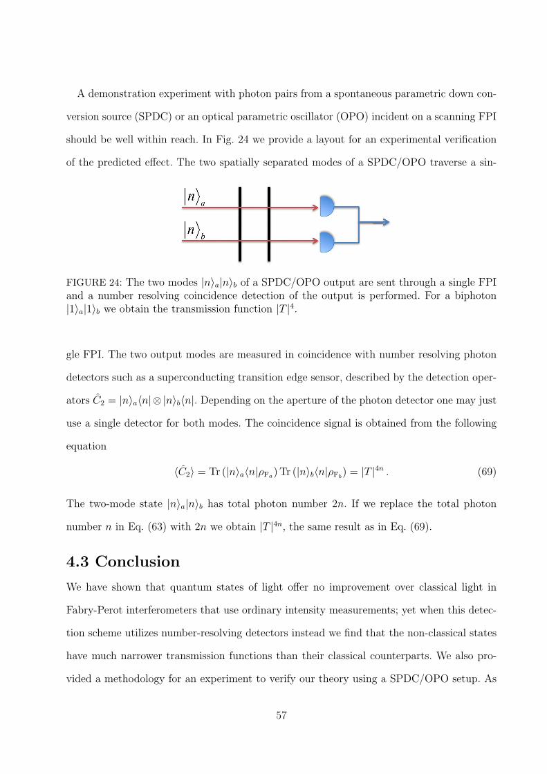
A demonstration experiment with photon pairs from a spontaneous parametric down con-
version source (SPDC) or an optical parametric oscillator (OPO) incident on a scanning FPI
should be well within reach. In Fig. 24 we provide a layout for an experimental verification
of the predicted effect. The two spatially separated modes of a SPDC/OPO traverse a sin-
FIGURE 24: The two modes |n〉a|n〉b of a SPDC/OPO output are sent through a single FPIand a number resolving coincidence detection of the output is performed. For a biphoton|1〉a|1〉b we obtain the transmission function |T |4.
gle FPI. The two output modes are measured in coincidence with number resolving photon
detectors such as a superconducting transition edge sensor, described by the detection oper-
ators C2 = |n〉a〈n|⊗ |n〉b〈n|. Depending on the aperture of the photon detector one may just
use a single detector for both modes. The coincidence signal is obtained from the following
equation
〈C2〉 = Tr (|n〉a〈n|ρFa) Tr (|n〉b〈n|ρFb) = |T |4n . (69)
The two-mode state |n〉a|n〉b has total photon number 2n. If we replace the total photon
number n in Eq. (63) with 2n we obtain |T |4n, the same result as in Eq. (69).
4.3 Conclusion
We have shown that quantum states of light offer no improvement over classical light in
Fabry-Perot interferometers that use ordinary intensity measurements; yet when this detec-
tion scheme utilizes number-resolving detectors instead we find that the non-classical states
have much narrower transmission functions than their classical counterparts. We also pro-
vided a methodology for an experiment to verify our theory using a SPDC/OPO setup. As
57
of this writing Allen Migdall of NIST and Christoph Wildfueuer of LSU have finished the
experiment proposed and will soon be submitting a paper on their findings.
Also of relevance, recently completed calculations by Jonathan Dowling and Christoph
Wildfueuer show that similarly, coherent states of light may show non-classical features when
measured by number resolving detectors. Those results combined with this chapter suggest
that there may be a large area of uncharted research in the examination of seemingly classical
states by non-classical detection methods.
58
5 Improving Optical Properties of Materialswith Photonic BandGap Coatings
Photonic Band Gap Materials are periodic dielectric or metallic structures that are designed
to alter the propagation of electromagnetic waves in an analogous fashion to a semiconduc-
tor’s affect on electron motion [90]. An overview is given into the optical properties, research
performed, and potential applications of such materials. My research is described in the area
of designing photonic crystals that have unique thermal emissivity properties and their ap-
plications to areas of research such as single photon sources and thermo-photovoltaic solar
energy conversion.
5.1 Introduction to Photonic Bandgap Materials
A crystal lattice is an arrangement of atoms or molecules that presents a periodic potential
to an electron propagating through it; the geometry of this arrangement determines many
of the bandgap properties, areas where propagation is limited. This knowledge has led to
the development of semiconductor technology, a 21st century revolution in our ability to
use physics to control microscopic properties of materials. In 1987, both Eli Yablonovitch
and Sajeev John independently proposed the idea to find materials that could produce
similar band gaps for electromagnetic radiation [91, 92]. Their goals were markedly different;
Yablonovitch, at Bell Labs, intended to find a way to reduce energy consumption in lasing,
where much of the electric current is wasted as spontaneous light emission, while John,
at Princeton, was pursuing a band gap which would lead to light localization. After an
experimental realization of the initial Photonic Crystal proposals, an influx of researchers
have come to the field to work on applications including communications, photovoltaic solar
energy, laser efficiency, medical lasers, and many more. These crystals have been built into 1,
2, and 3 dimensional structures, each with their own unique advantages and disadvantages for
various applications. One of the first recognizable applications was to create a new optical
fiber out of photonic crystal materials. These fibers are typically designed to have small
59
periodic holes of air in glass. The most common design has a triangular pattern of air holes,
with one hole missing in the center. In most cases the photonic crystal is made out of two
different periodic dielectric or metal materials; and in the 2 and 3-dimensional cases, the
geometry of the structure itself plays a crucial role in its properties.
The most common fabrication technique for creating photonic crystals, much like semi-
conductor chips, is lithography. Lithography is an efficient means of production for one
and two-dimensional structures, yet 3-dimensional structures become time-consuming and
very expensive for this process. Etching takes place on a micron scale, yet photonic crys-
tals are typically much larger than semiconductor chips; they’re on the order of millimeters
or centimeters for many applications. While incredibly accurate for building crystals and
adding defects, lithography becomes too cumbersome for large scale applications, such as
coating satellites. It appears unlikely that lithography will ever become practical for large
length-scales. A relatively recent advancement in large-scale fabrication has been to use the
idea of spontaneous crystallization, or self-assembly. The spontaneous crystallization of col-
loids (hard particles in suspension), provides an attractive alternative to the more time and
money intensive lithography method. While relatively cheap and much quicker, the downside
to self-assembly is in the control. Much of the ability to direct electromagnetic propagation
in photonic crystals comes from the carefully placed defects in the structure. While many
are skeptical about the number and type of defects that will be available to a self-assembly
process, its sheer ease of production make it an avenue worth pursuing.
There are several prominent methods for modeling the propagation of light through pho-
tonic crystals: plane-wave expansion, transfer matrices, and green’s functions represent the
three most frequently used. However green’s functions are quite cumbersome to work with,
leaving the first two options as the most desirable. Transfer matrices are for static cases
where the electromagnetic field doesn’t change with time. Plane-wave expansion methods
60
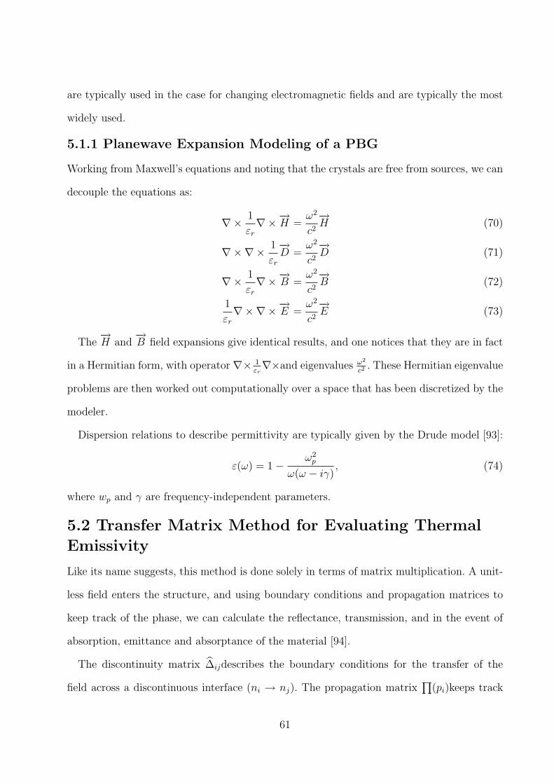
are typically used in the case for changing electromagnetic fields and are typically the most
widely used.
5.1.1 Planewave Expansion Modeling of a PBG
Working from Maxwell’s equations and noting that the crystals are free from sources, we can
decouple the equations as:
∇× 1
εr
∇×−→H =ω2
c2
−→H (70)
∇×∇× 1
εr
−→D =
ω2
c2
−→D (71)
∇× 1
εr
∇×−→B =ω2
c2
−→B (72)
1
εr
∇×∇×−→E =ω2
c2
−→E (73)
The−→H and
−→B field expansions give identical results, and one notices that they are in fact
in a Hermitian form, with operator ∇× 1εr∇×and eigenvalues ω2
c2. These Hermitian eigenvalue
problems are then worked out computationally over a space that has been discretized by the
modeler.
Dispersion relations to describe permittivity are typically given by the Drude model [93]:
ε(ω) = 1− ω2p
ω(ω − iγ), (74)
where wp and γ are frequency-independent parameters.
5.2 Transfer Matrix Method for Evaluating Thermal
Emissivity
Like its name suggests, this method is done solely in terms of matrix multiplication. A unit-
less field enters the structure, and using boundary conditions and propagation matrices to
keep track of the phase, we can calculate the reflectance, transmission, and in the event of
absorption, emittance and absorptance of the material [94].
The discontinuity matrix ∆ijdescribes the boundary conditions for the transfer of the
field across a discontinuous interface (ni → nj). The propagation matrix∏
(pi)keeps track
61
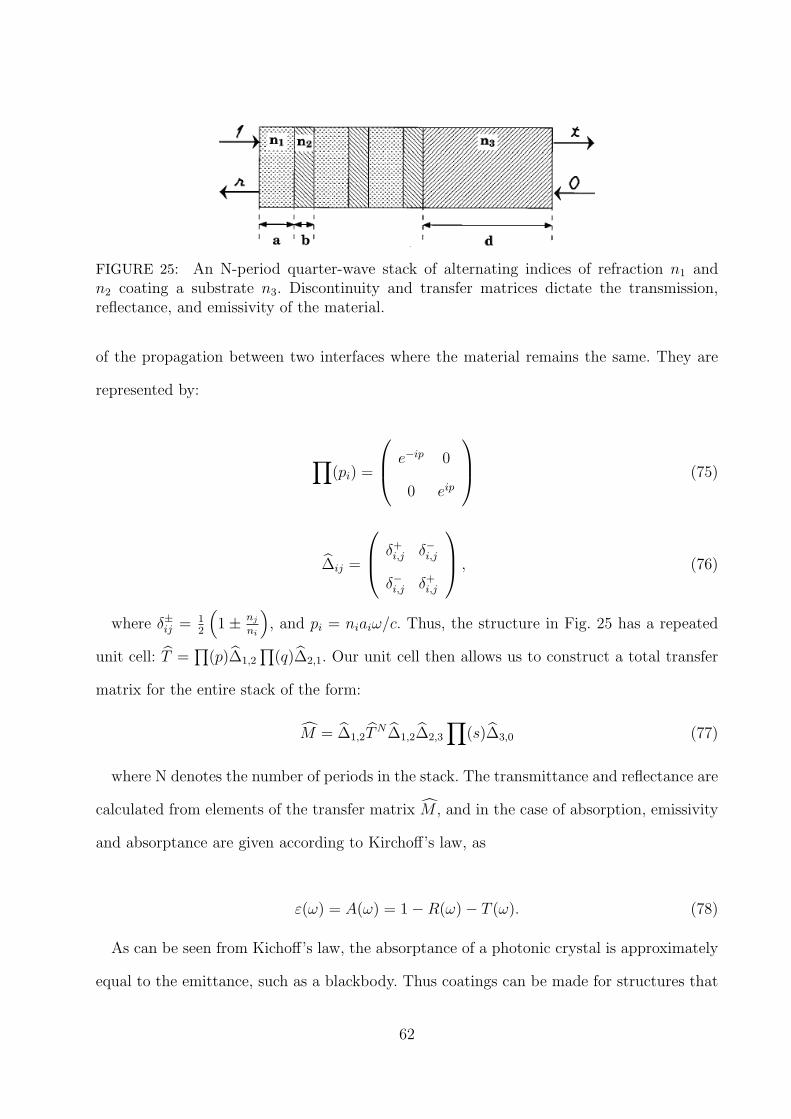
FIGURE 25: An N-period quarter-wave stack of alternating indices of refraction n1 andn2 coating a substrate n3. Discontinuity and transfer matrices dictate the transmission,reflectance, and emissivity of the material.
of the propagation between two interfaces where the material remains the same. They are
represented by:
∏(pi) =
e−ip 0
0 eip
(75)
∆ij =
δ+i,j δ−i,j
δ−i,j δ+i,j
, (76)
where δ±ij = 12
(1± nj
ni
), and pi = niaiω/c. Thus, the structure in Fig. 25 has a repeated
unit cell: T =∏
(p)∆1,2
∏(q)∆2,1. Our unit cell then allows us to construct a total transfer
matrix for the entire stack of the form:
M = ∆1,2TN∆1,2∆2,3
∏(s)∆3,0 (77)
where N denotes the number of periods in the stack. The transmittance and reflectance are
calculated from elements of the transfer matrix M , and in the case of absorption, emissivity
and absorptance are given according to Kirchoff’s law, as
ε(ω) = A(ω) = 1−R(ω)− T (ω). (78)
As can be seen from Kichoff’s law, the absorptance of a photonic crystal is approximately
equal to the emittance, such as a blackbody. Thus coatings can be made for structures that
62
selectively absorb less or more electromagnetic radiation in specified frequencies, with the
blackbody limit being the boundary. Practical applications for such a coating range from
reducing infra-red emittance of large buildings during winter, to lowering the absorptance of
solar radiation on satellites, to increasing the absorptance on solar cells.
5.3 Creating Photonic BandGap Coatings to Alter the
Emissive Properties of Materials
It has been the LSU Quantum Science and Technology group’s aim to create new ways of
designing photonic crystals for specified applications. Much of the current theory work in
the field revolves around discoveries of unique properties attributed to new and unique man-
made geometries. Thus, much of the design work involves intuition and luck, two attributes
that due not guarantee convergence to a solution.
In order to design and model new potential photonic bandgap materials, a process is desired
which is capable of optimization over a large parameter space. Our intent is to build such
a software process from the ground up using Genetic Algorithms (GA) as our optimization
technique, and emissivity as our target feature to design for. Our initial goal is a complete
1-dimensional design and modeling process, which gives qualitative 3-dimensional results as
per the John-Wang model [92], and then we plan to develop 2 and 3-dimensional design
programs.
GA’s work well in this capacity because of the large number of parameter possibilities, be
it layer lengths of the coating materials, variable ordering of the materials in the unit cell
(including the possibility of more than 2 materials), and the number of periods of the unit
cell. The flexibility of GA’s will further become essential in the 2 and 3-dimensional design
cases where the shapes of our structures have countless possible geometries, many of which
are difficult to predict before such an optimization process. The GA optimizes all tunable
variables to design a structure whose emissivity is iteratively closer to a desired emissivity
63
curve input from the designer. Many thousands of generations of designs can be created,
modeled, and then evolved towards a target solution.
Thermal management of satellites is an application ideally suited for this type of process.
We envision using this method to design a satellite PBG coating whose emissivity approaches
the blackbody limit in the IR, and is minimized in the Visible spectrum, so as to more effi-
ciently dispense with produced internal heat and lower the absorption of solar radiation. An
increase in satellite thermal efficiency will allow for higher power-density levels of operation
and for new satellite designs to have reduced size and weight.
Similarly, we hope for this process to aid in making solar cells more efficient by increasing
absorption across the spectrum emitted by the sun.
5.4 Preliminary Results of the Genetic Algorithm
At the time of this writing we have several proof of principle results to show that we may
numerically evolve structures that have desirable emissivity profiles. Starting from a point
of complete ignorance about how a structure is made, we use a desired emissivity as input,
and then our algorithm evolves a solution which matches our desired output as well as tells
us how to make the structure, i.e., the thickness of the different components of the repeating
structure as well as their indices of refraction.
As an example, we took Fig.26 from the Cornelius and Dowling paper to be our desired
emissivity profile.
After evolving two thousand generations of possible structure lengths with varying indices
of refraction our returned structure had a very similar emissivity profile, as can be seen
in Fig.27. What is interesting about this result is that it provides a very good match for
our desired emissivity, yet provides us with different indices of refraction. The immediate
suspicion is that there are many solutions in such a large search space that can provide
nearly identical results, and we may in fact achieve different solutions to the same problem
each time we run an analysis. While it is encouraging to know we can find a solution, the
64
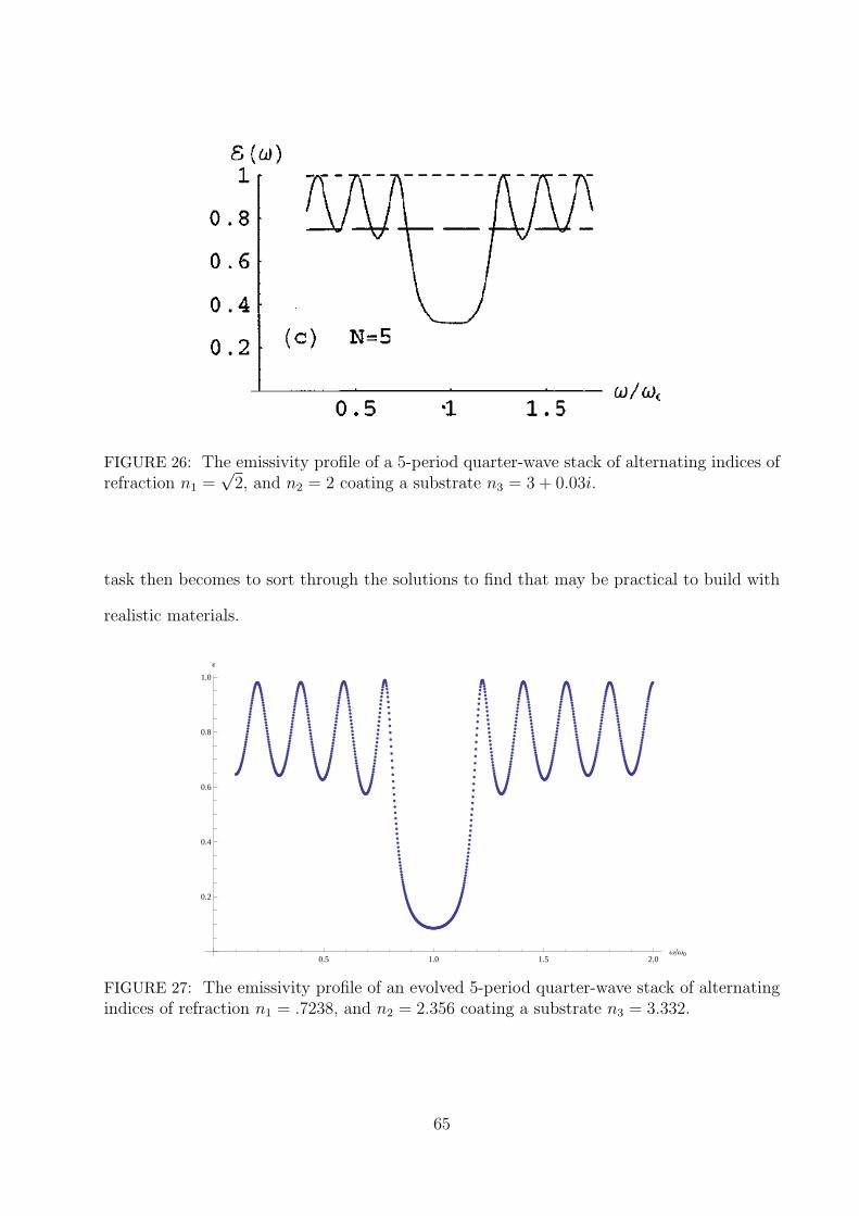
FIGURE 26: The emissivity profile of a 5-period quarter-wave stack of alternating indices ofrefraction n1 =
√2, and n2 = 2 coating a substrate n3 = 3 + 0.03i.
task then becomes to sort through the solutions to find that may be practical to build with
realistic materials.
0.5 1.0 1.5 2.0ΩΩ0
0.2
0.4
0.6
0.8
1.0
Ε
FIGURE 27: The emissivity profile of an evolved 5-period quarter-wave stack of alternatingindices of refraction n1 = .7238, and n2 = 2.356 coating a substrate n3 = 3.332.
65
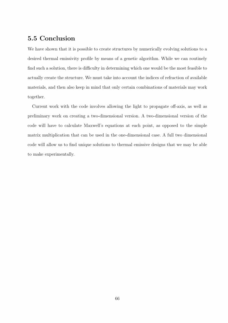
5.5 Conclusion
We have shown that it is possible to create structures by numerically evolving solutions to a
desired thermal emissivity profile by means of a genetic algorithm. While we can routinely
find such a solution, there is difficulty in determining which one would be the most feasible to
actually create the structure. We must take into account the indices of refraction of available
materials, and then also keep in mind that only certain combinations of materials may work
together.
Current work with the code involves allowing the light to propagate off-axis, as well as
preliminary work on creating a two-dimensional version. A two-dimensional version of the
code will have to calculate Maxwell’s equations at each point, as opposed to the simple
matrix multiplication that can be used in the one-dimensional case. A full two dimensional
code will allow us to find unique solutions to thermal emissive designs that we may be able
to make experimentally.
66
References
[1] J. Mehra, H. Rechenberg (1982). The Historical Development of Quantum Theory.New York: Springer-Verlag.
[2] T. Khun (1978). Black-Body Theory and the Quantum Discontinuity: 1894-1912. Ox-ford: Clarendon Press.
[3] M. Planck, Annalen der Physik, 4: 553 (1901).
[4] A. Einstein, Annalen der Physik, 17: 132-148 (1905).
[5] J.P. Gordon, H.J. Zeiger, and C.H. Townes, Phys. Rev. 95, 282 (1954).
[6] A.L. Schawlow, and C.H. Townes, Phys. Rev. 112, (1960).
[7] A. Einstein, Phys. Z. 18, 121-128,(1917).
[8] J.P. Dowling and G. Milburn, Philosophical Transactions of the Royal Society of Lon-don A, 361 (2003).
[9] H. Lee, P. Kok, and J. P. Dowling, J. Mod. Opt.,49,2325 (2002).
[10] V. Giovannetti, S. Lloyd, and L. Maccone, Science 306, 1330 (2004).
[11] A. L. Migdall, IEEE Trans. Instrum. Meas., 50, 478 (2001).
[12] E. Schrdinger, Die Naturwissenschaften 23 , 827 (1935).
[13] R. F. Werner, Phys. Rev. A, 40, 4277 (1989).
[14] J.S. Bell, Physics 1, 195 (1964).
[15] M. Genovese, Phys. Rep. 413, 319 (2005).
[16] N. Gisin and A. Peres, Phys. Lett. A 162, 15 (1992); S. Popescu and D. Rohrlich,Phys. Lett. A, 166, 293 (1992).
[17] C. F. Wildfeuer, A. P. Lund, and J. P. Dowling, Phys. Rev. A, 76, 052101 (2007).
[18] J. Fraden, Handbook of Modern Sensors, Springer-Verlag (1996).
[19] M. O. Scully and M. S. Zubairy, Quantum Optics, Cambridge University Press (1997).
[20] C. C. Gerry and P. L. Knight, Introductory Quantum Optics, Cambridge UniversityPress (2005).
[21] P. A. M. Dirac, Proc. Roy. Soc. A114, 243 (1927).
[22] W. Heitler, The Quantum Theory of Radiation, Oxford Unversity Press (1954).
67
[23] R. Loudon, The Quantum Thoery of Light, Oxford University Press (2000).
[24] C. M. Caves, Phys. Rev. D 23, 1693 (1981).
[25] D. Walls, Nature 306,141 (1983).
[26] M. Xiao, L.-A. Wu, H. J. Kimble, Phys. Rev. Lett. 59, 278 (1987).
[27] P.Grangier et al., Phys. Rev. Lett . 59, 2153 (1987).
[28] R. Loudon and P. L. Knight, J. Mod. Opt., 34, 709 (1987).
[29] A. S. Lane, S. L. Braunstein, and C. M. Caves, Phys. Rev. A 47, 1667 (1993).
[30] Z. Y. Ou, Phys. Rev. Lett. 77, 2352 (1996).
[31] V. V. Dodonov, J. Opt. B, 4, R1 (2002).
[32] T. Corbitt and N. Mavalvala, J. Opt. B, 6, S675 (2004).
[33] H.-A. Bachor and T. C. Ralph, A Guide to Experiments in Quantum Optics, 2ndedition (Wiley-VCH 2004).
[34] H. J. Kimble et al., Phys. Rev. D 65, 022002 (2001).
[35] J. Jacobson et al., Phys. Rev. Lett., 74, 4835 (1995).
[36] Y. Shih, IEEE J. Sel. Top. Quantum Electronics, 13, 1016 (2007).
[37] M. B. Nasr et al., Phys. Rev. Lett., 91, 083601 (2003).
[38] J. G. Rarity et al., Phys. Rev. Lett., 65, 1348 (1990).
[39] W. Boyd, Nonlinear Optics, 2nd edition (Academic Press, 2003).
[40] E. M. Nagasako et al., Phys. Rev. A, 64, 043802 (2001).
[41] G. S. Agarwal et al., J. Opt. Soc. Am. B, 24, 270 (2007).
[42] F. Scarrino et al., Phys. Rev. A, 77, 012324 (2008).
[43] P. W. Shor, Proc. 35th Annual Symposium on Foundations of Computer Science (ShafiGoldwasser, ed.),124-134, IEEE Computer Society Press (1994).
[44] C. H. Bennet and G. Brassard, Proceedings of the IEEE International Conference onComputers, Systems, and Signal Processing, Bangalore, p. 175 (1984).
[45] P. Neumann, et al., Science 320, 5881 (2008).
[46] E. Knill, R. Laflamme, and G.J. Milburn, Nature 409, 46 (2001).
[47] M. Reck, A. Zeilinger, H. J. Bernstein, and P. Bertani, Phys. Rev. Lett. 73, 58 (1994).
68
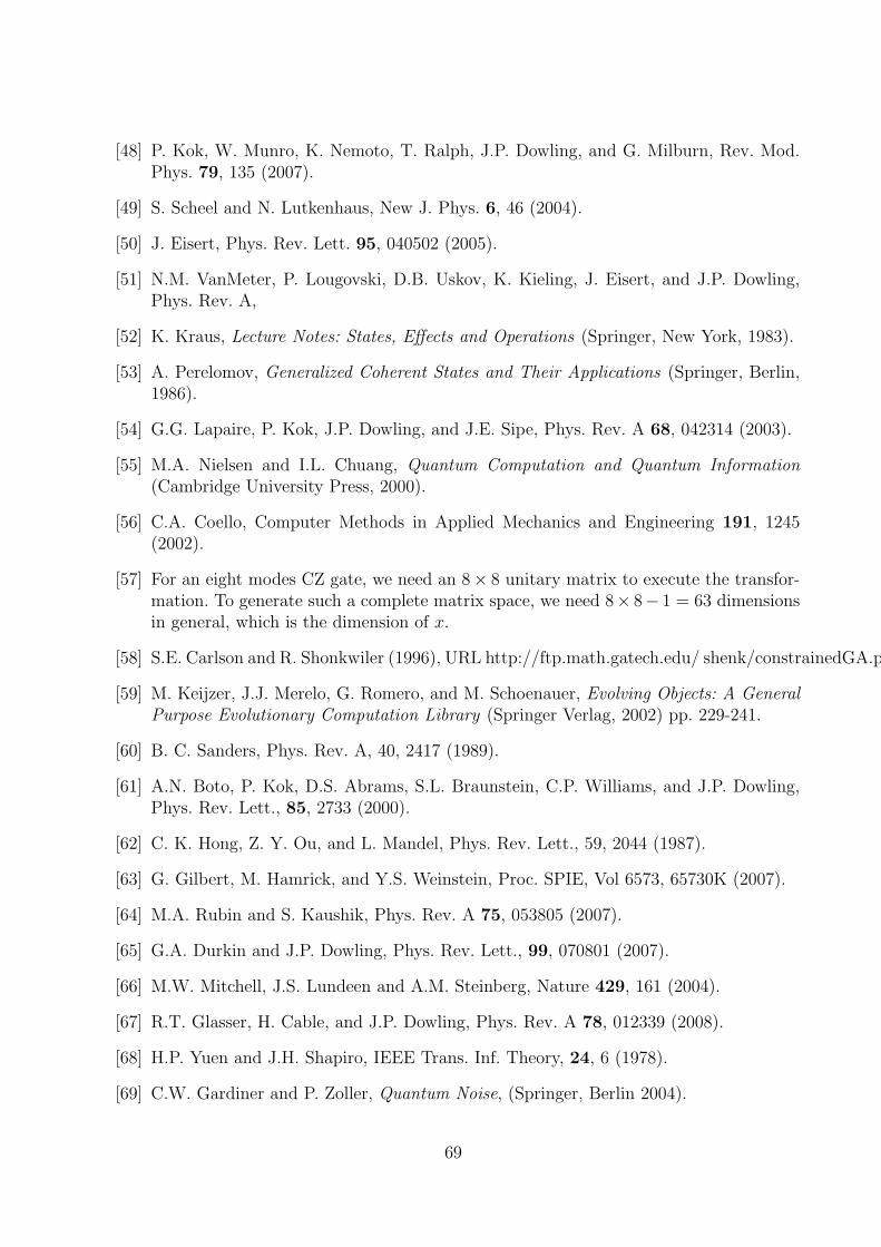
[48] P. Kok, W. Munro, K. Nemoto, T. Ralph, J.P. Dowling, and G. Milburn, Rev. Mod.Phys. 79, 135 (2007).
[49] S. Scheel and N. Lutkenhaus, New J. Phys. 6, 46 (2004).
[50] J. Eisert, Phys. Rev. Lett. 95, 040502 (2005).
[51] N.M. VanMeter, P. Lougovski, D.B. Uskov, K. Kieling, J. Eisert, and J.P. Dowling,Phys. Rev. A,
[52] K. Kraus, Lecture Notes: States, Effects and Operations (Springer, New York, 1983).
[53] A. Perelomov, Generalized Coherent States and Their Applications (Springer, Berlin,1986).
[54] G.G. Lapaire, P. Kok, J.P. Dowling, and J.E. Sipe, Phys. Rev. A 68, 042314 (2003).
[55] M.A. Nielsen and I.L. Chuang, Quantum Computation and Quantum Information(Cambridge University Press, 2000).
[56] C.A. Coello, Computer Methods in Applied Mechanics and Engineering 191, 1245(2002).
[57] For an eight modes CZ gate, we need an 8× 8 unitary matrix to execute the transfor-mation. To generate such a complete matrix space, we need 8× 8− 1 = 63 dimensionsin general, which is the dimension of x.
[58] S.E. Carlson and R. Shonkwiler (1996), URL http://ftp.math.gatech.edu/ shenk/constrainedGA.pdf
[59] M. Keijzer, J.J. Merelo, G. Romero, and M. Schoenauer, Evolving Objects: A GeneralPurpose Evolutionary Computation Library (Springer Verlag, 2002) pp. 229-241.
[60] B. C. Sanders, Phys. Rev. A, 40, 2417 (1989).
[61] A.N. Boto, P. Kok, D.S. Abrams, S.L. Braunstein, C.P. Williams, and J.P. Dowling,Phys. Rev. Lett., 85, 2733 (2000).
[62] C. K. Hong, Z. Y. Ou, and L. Mandel, Phys. Rev. Lett., 59, 2044 (1987).
[63] G. Gilbert, M. Hamrick, and Y.S. Weinstein, Proc. SPIE, Vol 6573, 65730K (2007).
[64] M.A. Rubin and S. Kaushik, Phys. Rev. A 75, 053805 (2007).
[65] G.A. Durkin and J.P. Dowling, Phys. Rev. Lett., 99, 070801 (2007).
[66] M.W. Mitchell, J.S. Lundeen and A.M. Steinberg, Nature 429, 161 (2004).
[67] R.T. Glasser, H. Cable, and J.P. Dowling, Phys. Rev. A 78, 012339 (2008).
[68] H.P. Yuen and J.H. Shapiro, IEEE Trans. Inf. Theory, 24, 6 (1978).
[69] C.W. Gardiner and P. Zoller, Quantum Noise, (Springer, Berlin 2004).
69
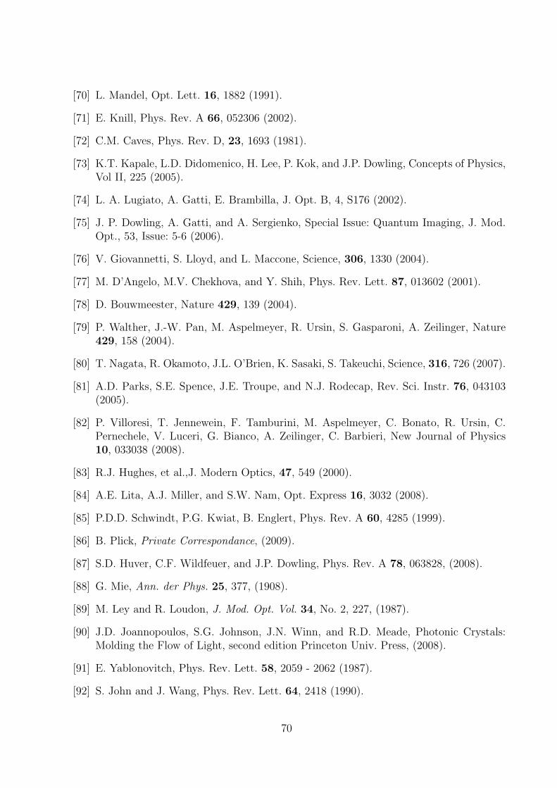
[70] L. Mandel, Opt. Lett. 16, 1882 (1991).
[71] E. Knill, Phys. Rev. A 66, 052306 (2002).
[72] C.M. Caves, Phys. Rev. D, 23, 1693 (1981).
[73] K.T. Kapale, L.D. Didomenico, H. Lee, P. Kok, and J.P. Dowling, Concepts of Physics,Vol II, 225 (2005).
[74] L. A. Lugiato, A. Gatti, E. Brambilla, J. Opt. B, 4, S176 (2002).
[75] J. P. Dowling, A. Gatti, and A. Sergienko, Special Issue: Quantum Imaging, J. Mod.Opt., 53, Issue: 5-6 (2006).
[76] V. Giovannetti, S. Lloyd, and L. Maccone, Science, 306, 1330 (2004).
[77] M. D’Angelo, M.V. Chekhova, and Y. Shih, Phys. Rev. Lett. 87, 013602 (2001).
[78] D. Bouwmeester, Nature 429, 139 (2004).
[79] P. Walther, J.-W. Pan, M. Aspelmeyer, R. Ursin, S. Gasparoni, A. Zeilinger, Nature429, 158 (2004).
[80] T. Nagata, R. Okamoto, J.L. O’Brien, K. Sasaki, S. Takeuchi, Science, 316, 726 (2007).
[81] A.D. Parks, S.E. Spence, J.E. Troupe, and N.J. Rodecap, Rev. Sci. Instr. 76, 043103(2005).
[82] P. Villoresi, T. Jennewein, F. Tamburini, M. Aspelmeyer, C. Bonato, R. Ursin, C.Pernechele, V. Luceri, G. Bianco, A. Zeilinger, C. Barbieri, New Journal of Physics10, 033038 (2008).
[83] R.J. Hughes, et al.,J. Modern Optics, 47, 549 (2000).
[84] A.E. Lita, A.J. Miller, and S.W. Nam, Opt. Express 16, 3032 (2008).
[85] P.D.D. Schwindt, P.G. Kwiat, B. Englert, Phys. Rev. A 60, 4285 (1999).
[86] B. Plick, Private Correspondance, (2009).
[87] S.D. Huver, C.F. Wildfeuer, and J.P. Dowling, Phys. Rev. A 78, 063828, (2008).
[88] G. Mie, Ann. der Phys. 25, 377, (1908).
[89] M. Ley and R. Loudon, J. Mod. Opt. Vol. 34, No. 2, 227, (1987).
[90] J.D. Joannopoulos, S.G. Johnson, J.N. Winn, and R.D. Meade, Photonic Crystals:Molding the Flow of Light, second edition Princeton Univ. Press, (2008).
[91] E. Yablonovitch, Phys. Rev. Lett. 58, 2059 - 2062 (1987).
[92] S. John and J. Wang, Phys. Rev. Lett. 64, 2418 (1990).
70
[93] J.D. Jackson, Classical Electrodynamics. New York: Wiley (1999).
[94] C.M. Cornelius and J.P. Dowling, Phys. Rev. A 59,4736-4746 , (1999).
71
Vita
Sean D. Huver was born in 1981, in St. Paul, Minnesota, to Prof. Charles W. Huver and
Ms. Rita M. DuCharme. He earned a bachelor of science degree in physics at the University
of California, Los Angeles, in May 2005. In August of 2005 he came to Louisiana State
University to pursue a Doctor of Philosophy degree in physics, specializing in quantum optics,
under the advisement of Prof. Jonathan P. Dowling, whom he had previously interned for
at NASA’s Jet Propulsion Laboratory. He is currently a doctoral candidate expecting to
graduate in May, 2009.
72