Embed Size (px)
Citation preview

Quantum Optics

D.F. Walls Gerard J. Milburn
Quantum Optics

D.F. Walls, F.R.S. Gerard J. Milburn(1942 – 1999) Physics Department
University of QueenslandSt Lucia, Brisbane QLD 4072, [email protected]
ISBN: 978-3-540-28573-1 e-ISBN: 978-3-540-28574-8
Library of Congress Control Number: 2007936291
c© 2008, 1994 Springer-Verlag Berlin Heidelberg
This work is subject to copyright. All rights are reserved, whether the whole or part of the material isconcerned, specifically the rights of translation, reprinting, reuse of illustrations, recitation, broadcasting,reproduction on microfilm or in any other way, and storage in data banks. Duplication of this publicationor parts thereof is permitted only under the provisions of the German Copyright Law of September 9,1965, in its current version, and permission for use must always be obtained from Springer. Violations areliable to prosecution under the German Copyright Law.
The use of general descriptive names, registered names, trademarks, etc. in this publication does not imply,even in the absence of a specific statement, that such names are exempt from the relevant protective lawsand regulations and therefore free for general use.
Cover design: eStudio Calamar S.L.
Printed on acid-free paper
9 8 7 6 5 4 3 2 1
springer.com

Preface to Second Edition
The field of quantum optics today is very different form the field that Dan Wallsand I surveyed in 1994 for the first Edition of this book. Some of the new fieldsthat have emerged over the years were hinted at in the earlier edition: quantuminformation has at least some roots in the study of Bell’s Inequalities, while the fieldsof ion trapping and quantum condensed gases have their roots in the old chapter onlight forces. However such is the growth of activity in each of these areas that Ihave found it necessary to write four new chapters for this edition. In order to keepthe book to a reasonable size this has meant cutting some of the material from thefirst edition. The old chapter on Intracavity Atomic Systems is largely gone withparts distributed in the new chapter on Cavity QED and elsewhere. Likewise the oldchapter on Resonance Fluorescence has been redistributed across Chaps. 10 and 11in this edition. No doubt more cutting could have been made but I have tried to keepsome continuity with the previous edition. In any case an emphasis on experimentalrealisations has been retained in the new material. Preparing this edition was not asmuch fun as the first. With Dan Walls untimely death in 1999, I have been deniedthe consolations of a shared task and soldiered on alone (although I must admit tohearing his voice from time to time as I cut and pasted). I can only hope that I havenot lost his vision for the book in my unchallenged role of sole author.
Brisbane, Australia, G.J. MilburnOctober 2007.
v

Contents
1 Introduction . . . . . . . . . . . . . . . . . . . . . . . . . . . . . . . . . . . . . . . . . . . . . . . . . . . 1
2 Quantisation of the Electromagnetic Field . . . . . . . . . . . . . . . . . . . . . . . . 72.1 Field Quantisation . . . . . . . . . . . . . . . . . . . . . . . . . . . . . . . . . . . . . . . . . . 72.2 Fock or Number States . . . . . . . . . . . . . . . . . . . . . . . . . . . . . . . . . . . . . . 102.3 Coherent States . . . . . . . . . . . . . . . . . . . . . . . . . . . . . . . . . . . . . . . . . . . . 122.4 Squeezed States . . . . . . . . . . . . . . . . . . . . . . . . . . . . . . . . . . . . . . . . . . . . 152.5 Two-Photon Coherent States . . . . . . . . . . . . . . . . . . . . . . . . . . . . . . . . . 182.6 Variance in the Electric Field . . . . . . . . . . . . . . . . . . . . . . . . . . . . . . . . . 202.7 Multimode Squeezed States . . . . . . . . . . . . . . . . . . . . . . . . . . . . . . . . . . 222.8 Phase Properties of the Field . . . . . . . . . . . . . . . . . . . . . . . . . . . . . . . . . 23Exercises . . . . . . . . . . . . . . . . . . . . . . . . . . . . . . . . . . . . . . . . . . . . . . . . . . . . . . 26References . . . . . . . . . . . . . . . . . . . . . . . . . . . . . . . . . . . . . . . . . . . . . . . . . . . . . 26Further Reading . . . . . . . . . . . . . . . . . . . . . . . . . . . . . . . . . . . . . . . . . . . . . . . . 27
3 Coherence Properties of the Electromagnetic Field . . . . . . . . . . . . . . . . . 293.1 Field-Correlation Functions . . . . . . . . . . . . . . . . . . . . . . . . . . . . . . . . . . 293.2 Properties of the Correlation Functions . . . . . . . . . . . . . . . . . . . . . . . . 313.3 Correlation Functions and Optical Coherence . . . . . . . . . . . . . . . . . . . 323.4 First-Order Optical Coherence . . . . . . . . . . . . . . . . . . . . . . . . . . . . . . . . 343.5 Coherent Field . . . . . . . . . . . . . . . . . . . . . . . . . . . . . . . . . . . . . . . . . . . . . 373.6 Photon Correlation Measurements . . . . . . . . . . . . . . . . . . . . . . . . . . . . 383.7 Quantum Mechanical Fields . . . . . . . . . . . . . . . . . . . . . . . . . . . . . . . . . . 41
3.7.1 Squeezed State . . . . . . . . . . . . . . . . . . . . . . . . . . . . . . . . . . . . . . 423.7.2 Squeezed Vacuum . . . . . . . . . . . . . . . . . . . . . . . . . . . . . . . . . . . 44
3.8 Phase-Dependent Correlation Functions . . . . . . . . . . . . . . . . . . . . . . . . 443.9 Photon Counting Measurements . . . . . . . . . . . . . . . . . . . . . . . . . . . . . . 46
3.9.1 Classical Theory . . . . . . . . . . . . . . . . . . . . . . . . . . . . . . . . . . . . . 463.9.2 Constant Intensity . . . . . . . . . . . . . . . . . . . . . . . . . . . . . . . . . . . . 483.9.3 Fluctuating Intensity–Short-Time Limit . . . . . . . . . . . . . . . . . 48
vii
viii Contents
3.10 Quantum Mechanical Photon Count Distribution . . . . . . . . . . . . . . . . 503.10.1 Coherent Light . . . . . . . . . . . . . . . . . . . . . . . . . . . . . . . . . . . . . . 513.10.2 Chaotic Light . . . . . . . . . . . . . . . . . . . . . . . . . . . . . . . . . . . . . . . 513.10.3 Photo-Electron Current Fluctuations . . . . . . . . . . . . . . . . . . . . 52
Exercises . . . . . . . . . . . . . . . . . . . . . . . . . . . . . . . . . . . . . . . . . . . . . . . . . . . . . . 54References . . . . . . . . . . . . . . . . . . . . . . . . . . . . . . . . . . . . . . . . . . . . . . . . . . . . . 55Further Reading . . . . . . . . . . . . . . . . . . . . . . . . . . . . . . . . . . . . . . . . . . . . . . . . 55
4 Representations of the Electromagnetic Field . . . . . . . . . . . . . . . . . . . . . . 574.1 Expansion in Number States . . . . . . . . . . . . . . . . . . . . . . . . . . . . . . . . . 574.2 Expansion in Coherent States . . . . . . . . . . . . . . . . . . . . . . . . . . . . . . . . . 58
4.2.1 P Representation . . . . . . . . . . . . . . . . . . . . . . . . . . . . . . . . . . . . . 584.2.2 Wigner’s Phase-Space Density . . . . . . . . . . . . . . . . . . . . . . . . . 624.2.3 Q Function . . . . . . . . . . . . . . . . . . . . . . . . . . . . . . . . . . . . . . . . . 654.2.4 R Representation . . . . . . . . . . . . . . . . . . . . . . . . . . . . . . . . . . . . 674.2.5 Generalized P Representations . . . . . . . . . . . . . . . . . . . . . . . . . 684.2.6 Positive P Representation . . . . . . . . . . . . . . . . . . . . . . . . . . . . . 71
Exercises . . . . . . . . . . . . . . . . . . . . . . . . . . . . . . . . . . . . . . . . . . . . . . . . . . . . . . 72References . . . . . . . . . . . . . . . . . . . . . . . . . . . . . . . . . . . . . . . . . . . . . . . . . . . . . 72
5 Quantum Phenomena in Simple Systems in Nonlinear Optics . . . . . . . 735.1 Single-Mode Quantum Statistics . . . . . . . . . . . . . . . . . . . . . . . . . . . . . . 73
5.1.1 Degenerate Parametric Amplifier . . . . . . . . . . . . . . . . . . . . . . . 735.1.2 Photon Statistics . . . . . . . . . . . . . . . . . . . . . . . . . . . . . . . . . . . . . 755.1.3 Wigner Function . . . . . . . . . . . . . . . . . . . . . . . . . . . . . . . . . . . . . 76
5.2 Two-Mode Quantum Correlations . . . . . . . . . . . . . . . . . . . . . . . . . . . . . 775.2.1 Non-degenerate Parametric Amplifier . . . . . . . . . . . . . . . . . . . 775.2.2 Squeezing . . . . . . . . . . . . . . . . . . . . . . . . . . . . . . . . . . . . . . . . . . 805.2.3 Quadrature Correlations and the Einstein–Podolsky–Rosen
Paradox . . . . . . . . . . . . . . . . . . . . . . . . . . . . . . . . . . . . . . . . . . . . 825.2.4 Wigner Function . . . . . . . . . . . . . . . . . . . . . . . . . . . . . . . . . . . . . 835.2.5 Reduced Density Operator . . . . . . . . . . . . . . . . . . . . . . . . . . . . 84
5.3 Quantum Limits to Amplification . . . . . . . . . . . . . . . . . . . . . . . . . . . . . 865.4 Amplitude Squeezed State with Poisson Photon Number Statistics . 88Exercises . . . . . . . . . . . . . . . . . . . . . . . . . . . . . . . . . . . . . . . . . . . . . . . . . . . . . . 91References . . . . . . . . . . . . . . . . . . . . . . . . . . . . . . . . . . . . . . . . . . . . . . . . . . . . . 91
6 Stochastic Methods . . . . . . . . . . . . . . . . . . . . . . . . . . . . . . . . . . . . . . . . . . . . . 936.1 Master Equation . . . . . . . . . . . . . . . . . . . . . . . . . . . . . . . . . . . . . . . . . . . 936.2 Equivalent c-Number Equations . . . . . . . . . . . . . . . . . . . . . . . . . . . . . . 99
6.2.1 Photon Number Representation . . . . . . . . . . . . . . . . . . . . . . . . 996.2.2 P Representation . . . . . . . . . . . . . . . . . . . . . . . . . . . . . . . . . . . . . 1006.2.3 Properties of Fokker–Planck Equations . . . . . . . . . . . . . . . . . . 1026.2.4 Steady State Solutions – Potential Conditions . . . . . . . . . . . . . 1036.2.5 Time Dependent Solution . . . . . . . . . . . . . . . . . . . . . . . . . . . . . 104

Contents ix
6.2.6 Q Representation . . . . . . . . . . . . . . . . . . . . . . . . . . . . . . . . . . . . 1056.2.7 Wigner Function . . . . . . . . . . . . . . . . . . . . . . . . . . . . . . . . . . . . . 1076.2.8 Generalized P Representation . . . . . . . . . . . . . . . . . . . . . . . . . . 109
6.3 Stochastic Differential Equations . . . . . . . . . . . . . . . . . . . . . . . . . . . . . 1126.3.1 Use of the Positive P Representation . . . . . . . . . . . . . . . . . . . . 115
6.4 Linear Processes with Constant Diffusion . . . . . . . . . . . . . . . . . . . . . . 1166.5 Two Time Correlation Functions in Quantum Markov Processes . . . 117
6.5.1 Quantum Regression Theorem . . . . . . . . . . . . . . . . . . . . . . . . . 1186.6 Application to Systems with a P Representation . . . . . . . . . . . . . . . . . 1186.7 Stochastic Unravellings . . . . . . . . . . . . . . . . . . . . . . . . . . . . . . . . . . . . . 119
6.7.1 Simulating Quantum Trajectories . . . . . . . . . . . . . . . . . . . . . . . 123Exercises . . . . . . . . . . . . . . . . . . . . . . . . . . . . . . . . . . . . . . . . . . . . . . . . . . . . . . 124References . . . . . . . . . . . . . . . . . . . . . . . . . . . . . . . . . . . . . . . . . . . . . . . . . . . . . 125Further Reading . . . . . . . . . . . . . . . . . . . . . . . . . . . . . . . . . . . . . . . . . . . . . . . . 125
7 Input–Output Formulation of Optical Cavities . . . . . . . . . . . . . . . . . . . . 1277.1 Cavity Modes . . . . . . . . . . . . . . . . . . . . . . . . . . . . . . . . . . . . . . . . . . . . . . 1277.2 Linear Systems . . . . . . . . . . . . . . . . . . . . . . . . . . . . . . . . . . . . . . . . . . . . 1317.3 Two-Sided Cavity . . . . . . . . . . . . . . . . . . . . . . . . . . . . . . . . . . . . . . . . . . 1327.4 Two Time Correlation Functions . . . . . . . . . . . . . . . . . . . . . . . . . . . . . . 1337.5 Spectrum of Squeezing . . . . . . . . . . . . . . . . . . . . . . . . . . . . . . . . . . . . . . 1357.6 Parametric Oscillator . . . . . . . . . . . . . . . . . . . . . . . . . . . . . . . . . . . . . . . 1367.7 Squeezing in the Total Field . . . . . . . . . . . . . . . . . . . . . . . . . . . . . . . . . . 1387.8 Fokker–Planck Equation . . . . . . . . . . . . . . . . . . . . . . . . . . . . . . . . . . . . . 138Exercises . . . . . . . . . . . . . . . . . . . . . . . . . . . . . . . . . . . . . . . . . . . . . . . . . . . . . . 141References . . . . . . . . . . . . . . . . . . . . . . . . . . . . . . . . . . . . . . . . . . . . . . . . . . . . . 141Further Reading . . . . . . . . . . . . . . . . . . . . . . . . . . . . . . . . . . . . . . . . . . . . . . . . 141
8 Generation and Applications of Squeezed Light . . . . . . . . . . . . . . . . . . . 1438.1 Parametric Oscillation and Second Harmonic Generation . . . . . . . . . 143
8.1.1 Semi-Classical Steady States and Stability Analysis . . . . . . . 1458.1.2 Parametric Oscillation . . . . . . . . . . . . . . . . . . . . . . . . . . . . . . . . 1468.1.3 Second Harmonic Generation . . . . . . . . . . . . . . . . . . . . . . . . . . 1468.1.4 Squeezing Spectrum . . . . . . . . . . . . . . . . . . . . . . . . . . . . . . . . . . 1478.1.5 Parametric Oscillation . . . . . . . . . . . . . . . . . . . . . . . . . . . . . . . . 1488.1.6 Experiments . . . . . . . . . . . . . . . . . . . . . . . . . . . . . . . . . . . . . . . . 149
8.2 Twin Beam Generation and Intensity Correlations . . . . . . . . . . . . . . . 1518.2.1 Second Harmonic Generation . . . . . . . . . . . . . . . . . . . . . . . . . . 1568.2.2 Experiments . . . . . . . . . . . . . . . . . . . . . . . . . . . . . . . . . . . . . . . . 157
8.3 Applications of Squeezed Light . . . . . . . . . . . . . . . . . . . . . . . . . . . . . . . 1588.3.1 Interferometric Detection of Gravitational Radiation . . . . . . . 1588.3.2 Sub-Shot-Noise Phase Measurements . . . . . . . . . . . . . . . . . . . 1718.3.3 Quantum Information . . . . . . . . . . . . . . . . . . . . . . . . . . . . . . . . . 173
Exercises . . . . . . . . . . . . . . . . . . . . . . . . . . . . . . . . . . . . . . . . . . . . . . . . . . . . . . 174

x Contents
References . . . . . . . . . . . . . . . . . . . . . . . . . . . . . . . . . . . . . . . . . . . . . . . . . . . . . 174Further Reading . . . . . . . . . . . . . . . . . . . . . . . . . . . . . . . . . . . . . . . . . . . . . . . . 175
9 Nonlinear Quantum Dissipative Systems . . . . . . . . . . . . . . . . . . . . . . . . . . 1779.1 Optical Parametric Oscillator: Complex P Function . . . . . . . . . . . . . . 1779.2 Optical Parametric Oscillator: Positive P Function . . . . . . . . . . . . . . . 1819.3 Quantum Tunnelling Time . . . . . . . . . . . . . . . . . . . . . . . . . . . . . . . . . . . 1869.4 Dispersive Optical Bistability . . . . . . . . . . . . . . . . . . . . . . . . . . . . . . . . 1909.5 Comment on the Use of the Q and Wigner Representations . . . . . . . . 192Exercises . . . . . . . . . . . . . . . . . . . . . . . . . . . . . . . . . . . . . . . . . . . . . . . . . . . . . . 1929.A Appendix . . . . . . . . . . . . . . . . . . . . . . . . . . . . . . . . . . . . . . . . . . . . . . . . . 193
9.A.1 Evaluation of Moments for the Complex P functionfor Parametric Oscillation (9.17) . . . . . . . . . . . . . . . . . . . . . . . 193
9.A.2 Evaluation of the Moments for the Complex P Functionfor Optical Bistability (9.48) . . . . . . . . . . . . . . . . . . . . . . . . . . . 194
References . . . . . . . . . . . . . . . . . . . . . . . . . . . . . . . . . . . . . . . . . . . . . . . . . . . . . 195Further Reading . . . . . . . . . . . . . . . . . . . . . . . . . . . . . . . . . . . . . . . . . . . . . . . . 195
10 Interaction of Radiation with Atoms . . . . . . . . . . . . . . . . . . . . . . . . . . . . . 19710.1 Quantization of the Many-Electron System . . . . . . . . . . . . . . . . . . . . . 19710.2 Interaction of a Single Two-Level Atom with a Single Mode Field . . 20110.3 Spontaneous Emission from a Two-Level Atom . . . . . . . . . . . . . . . . . 20310.4 Phase Decay in a Two-Level System . . . . . . . . . . . . . . . . . . . . . . . . . . . 20410.5 Resonance Fluorescence . . . . . . . . . . . . . . . . . . . . . . . . . . . . . . . . . . . . . 205Exercises . . . . . . . . . . . . . . . . . . . . . . . . . . . . . . . . . . . . . . . . . . . . . . . . . . . . . . 210References . . . . . . . . . . . . . . . . . . . . . . . . . . . . . . . . . . . . . . . . . . . . . . . . . . . . . 210Further Reading . . . . . . . . . . . . . . . . . . . . . . . . . . . . . . . . . . . . . . . . . . . . . . . . 211
11 CQED . . . . . . . . . . . . . . . . . . . . . . . . . . . . . . . . . . . . . . . . . . . . . . . . . . . . . . . . 21311.1 Cavity QED . . . . . . . . . . . . . . . . . . . . . . . . . . . . . . . . . . . . . . . . . . . . . . . 213
11.1.1 Vacuum Rabi Splitting . . . . . . . . . . . . . . . . . . . . . . . . . . . . . . . . 21711.1.2 Single Photon Sources . . . . . . . . . . . . . . . . . . . . . . . . . . . . . . . . 21811.1.3 Cavity QED with N Atoms . . . . . . . . . . . . . . . . . . . . . . . . . . . . 221
11.2 Circuit QED . . . . . . . . . . . . . . . . . . . . . . . . . . . . . . . . . . . . . . . . . . . . . . . 225Exercises . . . . . . . . . . . . . . . . . . . . . . . . . . . . . . . . . . . . . . . . . . . . . . . . . . . . . . 227References . . . . . . . . . . . . . . . . . . . . . . . . . . . . . . . . . . . . . . . . . . . . . . . . . . . . . 228Further Reading . . . . . . . . . . . . . . . . . . . . . . . . . . . . . . . . . . . . . . . . . . . . . . . . 229
12 Quantum Theory of the Laser . . . . . . . . . . . . . . . . . . . . . . . . . . . . . . . . . . . 23112.1 Master Equation . . . . . . . . . . . . . . . . . . . . . . . . . . . . . . . . . . . . . . . . . . . 23112.2 Photon Statistics . . . . . . . . . . . . . . . . . . . . . . . . . . . . . . . . . . . . . . . . . . . 233
12.2.1 Spectrum of Intensity Fluctuations . . . . . . . . . . . . . . . . . . . . . . 23412.3 Laser Linewidth . . . . . . . . . . . . . . . . . . . . . . . . . . . . . . . . . . . . . . . . . . . . 23712.4 Regularly Pumped Laser . . . . . . . . . . . . . . . . . . . . . . . . . . . . . . . . . . . . 23812.A Appendix: Derivation of the Single-Atom Increment . . . . . . . . . . . . . 242
Contents xi
Exercises . . . . . . . . . . . . . . . . . . . . . . . . . . . . . . . . . . . . . . . . . . . . . . . . . . . . . . 245References . . . . . . . . . . . . . . . . . . . . . . . . . . . . . . . . . . . . . . . . . . . . . . . . . . . . . 245
13 Bells Inequalities in Quantum Optics . . . . . . . . . . . . . . . . . . . . . . . . . . . . . 24713.1 The Einstein–Podolsky–Rosen (EPR) Argument . . . . . . . . . . . . . . . . . 24713.2 Bell Inequalities and the Aspect Experiment . . . . . . . . . . . . . . . . . . . . 24813.3 Violations of Bell’s Inequalities Using a Parametric Amplifier
Source . . . . . . . . . . . . . . . . . . . . . . . . . . . . . . . . . . . . . . . . . . . . . . . . . . . . 25413.4 One-Photon Interference . . . . . . . . . . . . . . . . . . . . . . . . . . . . . . . . . . . . . 259Exercises . . . . . . . . . . . . . . . . . . . . . . . . . . . . . . . . . . . . . . . . . . . . . . . . . . . . . . 264References . . . . . . . . . . . . . . . . . . . . . . . . . . . . . . . . . . . . . . . . . . . . . . . . . . . . . 264
14 Quantum Nondemolition Measurements . . . . . . . . . . . . . . . . . . . . . . . . . . 26714.1 Concept of a QND Measurement . . . . . . . . . . . . . . . . . . . . . . . . . . . . . . 26814.2 Back Action Evasion . . . . . . . . . . . . . . . . . . . . . . . . . . . . . . . . . . . . . . . . 27014.3 Criteria for a QND Measurement . . . . . . . . . . . . . . . . . . . . . . . . . . . . . 27014.4 The Beam Splitter . . . . . . . . . . . . . . . . . . . . . . . . . . . . . . . . . . . . . . . . . . 27314.5 Ideal Quadrature QND Measurements . . . . . . . . . . . . . . . . . . . . . . . . . 27614.6 Experimental Realisation . . . . . . . . . . . . . . . . . . . . . . . . . . . . . . . . . . . . 27714.7 A Photon Number QND Scheme . . . . . . . . . . . . . . . . . . . . . . . . . . . . . . 279Exercises . . . . . . . . . . . . . . . . . . . . . . . . . . . . . . . . . . . . . . . . . . . . . . . . . . . . . . 281References . . . . . . . . . . . . . . . . . . . . . . . . . . . . . . . . . . . . . . . . . . . . . . . . . . . . . 282
15 Quantum Coherence and Measurement Theory . . . . . . . . . . . . . . . . . . . 28315.1 Quantum Coherence . . . . . . . . . . . . . . . . . . . . . . . . . . . . . . . . . . . . . . . . 28315.2 The Effect of Dissipation . . . . . . . . . . . . . . . . . . . . . . . . . . . . . . . . . . . . 288
15.2.1 Experimental Observation of Coherence Decay . . . . . . . . . . . 29115.3 Quantum Measurement Theory . . . . . . . . . . . . . . . . . . . . . . . . . . . . . . . 293
15.3.1 General Measurement Theory . . . . . . . . . . . . . . . . . . . . . . . . . . 29415.3.2 The Pointer Basis . . . . . . . . . . . . . . . . . . . . . . . . . . . . . . . . . . . . 296
15.4 Examples of Pointer Observables . . . . . . . . . . . . . . . . . . . . . . . . . . . . . 29915.5 Model of a Measurement . . . . . . . . . . . . . . . . . . . . . . . . . . . . . . . . . . . . 29915.6 Conditional States and Quantum Trajectories . . . . . . . . . . . . . . . . . . . 302
15.6.1 Homodyne Measurement of a Cavity Field . . . . . . . . . . . . . . . 303Exercises . . . . . . . . . . . . . . . . . . . . . . . . . . . . . . . . . . . . . . . . . . . . . . . . . . . . . . 305References . . . . . . . . . . . . . . . . . . . . . . . . . . . . . . . . . . . . . . . . . . . . . . . . . . . . . 306
16 Quantum Information . . . . . . . . . . . . . . . . . . . . . . . . . . . . . . . . . . . . . . . . . . 30716.1 Introduction . . . . . . . . . . . . . . . . . . . . . . . . . . . . . . . . . . . . . . . . . . . . . . . 307
16.1.1 The Qubit . . . . . . . . . . . . . . . . . . . . . . . . . . . . . . . . . . . . . . . . . . 30816.1.2 Entanglement . . . . . . . . . . . . . . . . . . . . . . . . . . . . . . . . . . . . . . . 310
16.2 Quantum Key Distribution . . . . . . . . . . . . . . . . . . . . . . . . . . . . . . . . . . . 31216.3 Quantum Teleportation . . . . . . . . . . . . . . . . . . . . . . . . . . . . . . . . . . . . . . 31816.4 Quantum Computation . . . . . . . . . . . . . . . . . . . . . . . . . . . . . . . . . . . . . . 324
16.4.1 Linear Optical Quantum Gates . . . . . . . . . . . . . . . . . . . . . . . . . 32716.4.2 Single Photon Sources . . . . . . . . . . . . . . . . . . . . . . . . . . . . . . . . 336
Exercises . . . . . . . . . . . . . . . . . . . . . . . . . . . . . . . . . . . . . . . . . . . . . . . . . . . . . . 343
xii Contents
References . . . . . . . . . . . . . . . . . . . . . . . . . . . . . . . . . . . . . . . . . . . . . . . . . . . . . 344Further Reading . . . . . . . . . . . . . . . . . . . . . . . . . . . . . . . . . . . . . . . . . . . . . . . . 346
17 Ion Traps . . . . . . . . . . . . . . . . . . . . . . . . . . . . . . . . . . . . . . . . . . . . . . . . . . . . . 34717.1 Introduction . . . . . . . . . . . . . . . . . . . . . . . . . . . . . . . . . . . . . . . . . . . . . . . 34717.2 Trapping and Cooling . . . . . . . . . . . . . . . . . . . . . . . . . . . . . . . . . . . . . . . 34717.3 Novel Quantum States . . . . . . . . . . . . . . . . . . . . . . . . . . . . . . . . . . . . . . 35317.4 Trapping Multiple Ions . . . . . . . . . . . . . . . . . . . . . . . . . . . . . . . . . . . . . . 35617.5 Ion Trap Quantum Information Processing . . . . . . . . . . . . . . . . . . . . . 359Exercises . . . . . . . . . . . . . . . . . . . . . . . . . . . . . . . . . . . . . . . . . . . . . . . . . . . . . . 362References . . . . . . . . . . . . . . . . . . . . . . . . . . . . . . . . . . . . . . . . . . . . . . . . . . . . . 363
18 Light Forces . . . . . . . . . . . . . . . . . . . . . . . . . . . . . . . . . . . . . . . . . . . . . . . . . . . 36518.1 Radiative Forces in the Semiclassical Limit . . . . . . . . . . . . . . . . . . . . 36618.2 Mean Force for a Two–Level Atom Initially at Rest . . . . . . . . . . . . . . 36818.3 Friction Force for a Moving Atom . . . . . . . . . . . . . . . . . . . . . . . . . . . . 371
18.3.1 Laser Standing Wave—Doppler Cooling . . . . . . . . . . . . . . . . . 37218.4 Dressed State Description of the Dipole Force . . . . . . . . . . . . . . . . . . 37418.5 Atomic Diffraction by a Standing Wave . . . . . . . . . . . . . . . . . . . . . . . . 37718.6 Optical Stern–Gerlach Effect . . . . . . . . . . . . . . . . . . . . . . . . . . . . . . . . . 38118.7 Quantum Chaos . . . . . . . . . . . . . . . . . . . . . . . . . . . . . . . . . . . . . . . . . . . . 385
18.7.1 Dynamical Tunnelling . . . . . . . . . . . . . . . . . . . . . . . . . . . . . . . . 38718.7.2 Dynamical Localisation . . . . . . . . . . . . . . . . . . . . . . . . . . . . . . . 389
18.8 The Effect of Spontaneous Emission . . . . . . . . . . . . . . . . . . . . . . . . . . 390References . . . . . . . . . . . . . . . . . . . . . . . . . . . . . . . . . . . . . . . . . . . . . . . . . . . . . 394Further Reading . . . . . . . . . . . . . . . . . . . . . . . . . . . . . . . . . . . . . . . . . . . . . . . . 395
19 Bose-Einstein Condensation . . . . . . . . . . . . . . . . . . . . . . . . . . . . . . . . . . . . . 39719.1 Hamiltonian: Binary Collision Model . . . . . . . . . . . . . . . . . . . . . . . . . . 39819.2 Mean–Field Theory — Gross-Pitaevskii Equation . . . . . . . . . . . . . . 39919.3 Single Mode Approximation . . . . . . . . . . . . . . . . . . . . . . . . . . . . . . . . 40019.4 Quantum State of the Condensate . . . . . . . . . . . . . . . . . . . . . . . . . . . . 40119.5 Quantum Phase Diffusion: Collapses
and Revivals of the Condensate Phase . . . . . . . . . . . . . . . . . . . . . . . . . 40119.6 Interference of Two Bose–Einstein Condensates
and Measurement–Induced Phase . . . . . . . . . . . . . . . . . . . . . . . . . . . . . 40519.6.1 Interference of Two Condensates Initially in Number
States . . . . . . . . . . . . . . . . . . . . . . . . . . . . . . . . . . . . . . . . . . . . . 40519.7 Quantum Tunneling of a Two Component Condensate . . . . . . . . . . . . 409
19.7.1 Semiclassical Dynamics . . . . . . . . . . . . . . . . . . . . . . . . . . . . . . 41119.7.2 Quantum Dynamics . . . . . . . . . . . . . . . . . . . . . . . . . . . . . . . . . . 414
19.8 Coherence Properties of Bose–Einstein Condensates . . . . . . . . . . . . . 41619.8.1 1st Order Coherence . . . . . . . . . . . . . . . . . . . . . . . . . . . . . . . . . . 41619.8.2 Higher Order Coherence . . . . . . . . . . . . . . . . . . . . . . . . . . . . . . 417
Exercises . . . . . . . . . . . . . . . . . . . . . . . . . . . . . . . . . . . . . . . . . . . . . . . . . . . . . . 419References . . . . . . . . . . . . . . . . . . . . . . . . . . . . . . . . . . . . . . . . . . . . . . . . . . . . . 419Further Reading . . . . . . . . . . . . . . . . . . . . . . . . . . . . . . . . . . . . . . . . . . . . . . . . 420
Index . . . . . . . . . . . . . . . . . . . . . . . . . . . . . . . . . . . . . . . . . . . . . . . . . . . . . . . . . . . . . 421

Chapter 1Introduction
The first indication of the quantum nature of light came in 1900 when Planck dis-covered he could account for the spectral distribution of thermal light by postulatingthat the energy of a simple harmonic oscillator was quantized. Further evidence wasadded by Einstein who showed in 1905 that the photoelectric effect could be ex-plained by the hypothesis that the energy of a light beam was distributed in discretepackets later known as photons.
Einstein also contributed to the understanding of the absorption and emissionof light from atoms with his development of a phenomenological theory in 1917.This theory was later shown to be a natural consequence of the quantum theory ofelectromagnetic radiation.
Despite this early connection with the quantum theory, physical optics developedmore or less independently of quantum theory. The vast majority of physical-opticsexperiments can be adequately explained using classical theory of electromagnetismbased on Maxwell’s equations. An early attempt to find quantum effects in an op-tical interference experiment by G.I. Taylor in 1909 gave a negative result. Tay-lor’s experiment was an attempt to repeat Young’s famous two slit experiment withone photon incident on the slits. The classical explanation based in the interfer-ence of electric field amplitudes and the quantum explanation based on the inter-ference of probability amplitudes both correctly explain the phenomenon in thisexperiment. Interference experiments of Young’s type do not distinguish betweenthe predictions of the classical theory and the quantum theory. It is only in higherorder interference experiments, involving the interference of intensities, that differ-ences between the predictions of classical and quantum theory appear. In such anexperiment the probability amplitudes to detect a photon from two different fieldsinterfere on a detector. Whereas classical theory treats the interference of intensi-ties, in quantum theory the interference is still at the level of probability amplitudes.This is one of the most important differences between the classical and the quantumtheory.
The first experiment in intensity interferometry was the famous experiment ofR. Hanbury Brown and R.Q. Twiss. This experiment studied the correlation in the
1
2 1 Introduction
photocurrent fluctuations fro two detectors. Later experiments were based on photoncounting, and the correlation between photon number was studied.
The Hanbury–Brown and Twiss experiment observed an enhancement in the two-time correlation function of short time delays for a thermal light source, known asphoton bunching. This was a consequence of the large intensity fluctuations in thethermal source. Such photon bunching phenomenon may be adequately explainedusing a classical theory with a fluctuating electric field amplitude. For a perfectlyamplitude stabilized light field, such as an ideal laser operating well above thresh-old, there is no photon bunching. A photon counting experiment where the numberof photons arriving in an interval of time T are counted, shows that there is stillrandomness in the arrival time of the photons. The photon number distribution foran ideal laser is Poissonian. For thermal light a super-Poissonian photocount distri-bution results.
While the these results may be derived form a classical and quantum theory,the quantum theory makes additional unique predictions. This was first elucidatedby R.J. Glauber in his quantum formulation of optical coherence theory in 1963.Glauber was jointly awarded the 2005 Nobel Prize in physics for this work. Onesuch prediction is photon anti bunching, in which the initial slope of the two-timephoton correlation function is positive. This corresponds to an enhancement, onaverage, of the temporal separation between photo counts at a detector, or photonanti-bunching. The photo-count statistics may also be sub-Poissonian. A classicaltheory of fluctuating field amplitudes would require negative probability in orderto give anti-bunching. In the quantum picture it is easy to visualize photon arrivalsmore regular than Poissonian.
It was not until 1975 that H.J. Carmichel and D.F. Walls predicted that lightgenerated in resonance fluorescence fro a two-level atom would exhibit photon anti-bunching that a physically accessible system exhibiting non-classical behaviour wasidentified. Photon anti-bunching in this system was observed the following year byH.J. Kimble, M. Dagenais and L. Mandel. This was the first non classical effectobserved in optics and ushered in a new era of quantum optics.
The experiments of Kimble et al. used an atomic beam and hence the photonanti-bunching was convoluted with the atomic number fluctuations in the beam.With the development of ion trap technology it is now possible to trap a single ionfor many minute and observe fluorescence. H. Walther and co workers in Munichhave studied resonance fluorescence from a single ion in a trap and observed bothphoton bunching and anti-bunching.
In the 1960s improvements in photon counting techniques proceeded in tandemwith the development of new laser light sources. Light from incoherent (thermal)and coherent (laser) sources could now be distinguished by their photon count-ing statistics. The groups of F.T. Arecchi in Milan, L. Mandel in Rochester andR. Pike in Malvern measured the photo count statistics of the laser. These exper-iments showed that the photo-count statistics went from super-Poissonian belowthreshold to Poissonian far above threshold. Concurrently the quantum theory ofthe laser was being developed by H. Haken in Stuttgart, M.O. Scully and W. Lambin Yale and M. Lax and W.H. Louisell in New Jersey. In these theories both the

1 Introduction 3
atomic variables and the electromagnetic field were quantized. The results of thesecalculations were that the laser functioned as an essentially classical device. In factH. Risken showed that it could be modeled as a van der Pol Oscillator.
In the late 80s the role of noise in the laser pumping process was shown to ob-scure the quantum aspects of the laser. If the noise in the pump can be suppressedthe laser may exhibit sub-Poissonian statistics. In other words the intensity fluctu-ations may be reduced below the shot noise level of normal lasers. Y. Yamamotofirst in Tokyo and then Stanford has pioneered experimental developments of semi-conductor lasers with suppressed pump noise. More recently, Yamamoto and othershave pioneered the development of the single photon source. This is a source oftransform-limited pulsed light with one and only one photon per pulse: the ultimatelimit of an anti-bunched source. The average field amplitude of such a source iszero while the intensity is definite. Such sources are highly non classical and haveapplications in quantum communication and computation.
It took another nine years after the first observation of photon anti-bunching foranother prediction of the quantum theory of light to be observed – squeezing ofquantum fluctuations. The electric field of a nearly monochromatic plane wave maybe decomposed into two quadrature component amplitudes of an oscillatory sineterm and a cosine term. In a coherent state, the closest quantum counter-part toa classical field, the fluctuations in the two quadrature amplitudes are equal andsaturate the lower bound in the Heisenberg uncertainty relation. The quantum fluc-tuations in a coherent state are equal to the zero point fluctuations of the vacuumand are randomly distributed in phase. In a squeezed state the fluctuations are phasedependent. One quadrature phase amplitude may have reduced fluctuations com-pared to the vacuum while, in consequence, the other quadrature phase amplitudewill have increased fluctuations, with the product of the uncertainties still saturatingthe lower bound in the Heisenberg uncertainty relation.
The first observation of squeezed light was made by R.E. Slusher in 1985 atAT&T Bell Laboratories in four wave mixing. Shortly after squeezing was demon-strated using optical parametric oscillators, by H.J. Kimble and four wave mixingin optical fibres by M.D. Levenson. Since then, greater and greater degrees of quan-tum noise suppression have been demonstrated, currently more than 7 dB, drivenby new applications in quantum communication protocols such as teleportation andcontinuous variable quantum key distribution.
In the nonlinear process of parametric down conversion, a high frequency photonis absorbed and two photons are simultaneously produced with lower frequencies.The two photons produced are correlated in frequency, momentum and possiblypolarisation. This results in very strong intensity correlations in the down convertedbeams that results in strongly suppressed intensity difference fluctuations as demon-strated by E. Giacobino in Paris and P. Kumar in Evanston.
Early uses of such correlated twin beams included accurate absorption measure-ments in which the sample was placed in one arm with the other beam providinga reference. when the twin beams are detected and the photo currents are sub-tracted, the presence of very weak absorption can be seen because of the small quan-tum noise in the difference current. More recently the strong intensity correlations

4 1 Introduction
have been used to provide an accurate calibration of photon detector efficiency byA. Migdall at NIST and also in so called quantum imaging in which an object pacedin one path changes the spatial pattern of intensity correlations between the twotwin beams.
The high degree of correlation between the down converted photons enablessome of the most stringent demonstrations of the violation of the Bell inequalitiesin quantum physics. In 1999 P. Kwiat obtained a violation by more than 240 stan-dard deviations using polarisation correlated photons produced by type II parametricdown conversion. The quadrature phase amplitudes in the twin beams generated indown conversion carry quantum correlations of the Einstein-Podolsky-Rosen type.This enabled the continuous variable version of quantum teleportation, proposed byL. Vaidmann, to be demonstrated by H.J. Kimble in 1998. More recently P.K. Lam,using the same quadrature phase correlations, demonstrated a continuous variablequantum key distributions.
These last examples lie at the intersection of quantum optics with the new fieldof quantum information. Quantum entanglement enables new communication andcomputational tasks to be performed that are either difficult or impossible in a classi-cal world. Quantum optics provides an ideal test bed for experimental investigationsin quantum information, and such investigations now form a large part of the exper-imental agenda in the field.
Quantum optics first entered the business of quantum information processingwith the proposal of Cirac and Zoller in 1995 to use ion trap technology. Fol-lowing pioneering work by Dehmelt and others using ion traps for high resolu-tion spectroscopy, by the early 1990s it was possible to trap and cool a single ionto almost the ground state of its vibrational motion. Cirac and Zoller proposed ascheme, using multiple trapped ions, by which quantum information stored in theinternal electronic state of each ion could be processed using an external laser tocorrelate the internal states of different ions using collective vibrational degrees offreedom. Ion traps currently provide the most promising approach to quantum in-formation processing with more than eight qubits having been entangled in the labsof D. Wineland at NIST in Colorado and R. Blatt in Innsbruck.
Quantum computation requires the ability to strongly entangle independent de-grees of freedom that are used to encode information, known as qubits. It was ini-tially thought however that the very weak optical nonlinearities typically found inquantum optics would not be powerful enough to implement such entangling opera-tions. This changed in 2001 when E. Knill, R. Laflamme and G.J. Milburn, followedshortly thereafter by T. Pittman and J. Franson, proposed a way to perform condi-tional entangling operations using information encoded on single photons, and pho-ton counting measurements. Early experimental demonstrations of simple quantumgates soon followed.
At about the same time another measurement based protocol for quantum com-puting was devised by R. Raussendorf and H. Breigel. Nielsen showed how this ap-proach could be combined with the single photon methods introduced by Knill et al.,to dramatically simplify the implementation of conditional gates. The power of thisapproach was recently demonstrated by A. Zeilinger’s group in Vienna. Scaling up

1 Introduction 5
this approach to more and more qubits is a major activity of experimental quantumoptics.
These schemes provide a powerful incentive to develop a totally new kind of lightsource: the single photon pulsed source. This is a pulsed light source that producesone and only one photon per pulse. Such sources are in development in many labo-ratories around the world. A variety of approaches are being pursued. Sources basedon excitons in semiconductor quantum dots are being developed by A. Imamogluin Zurich, A. Shields in Toshiba Cambridge, and Y. Yamamoto and J. Vukovic inStanford. NV centres in diamond nanocrystal are under development by S. Prawerin Melbourne. An interesting approach based on down conversion in optical fibersis being studied by A. Migdall in NIST. Sources based on single atoms in opticalcavities have been demonstrated by H. Walther in Munich and P. Grangier in Paris.Once routinely available, single photon sources will enable a new generation of ex-periments in single photon quantum optics.
Beginning in the early 1980s a number of pioneers including G. Ashkin, C. CohenTannoudji and S. Chu began to study the forces exerted on atoms by light. This workled to the ability to cool and trap ensembles of atoms, or even single atoms, and cul-minated in the experimental demonstration by E. Cornell and C. Weimann of a BoseEinstein condensate using a dilute gas of rubidium atoms at NIST in 1995, followedsoon thereafter by W. Ketterle at Harvard. Discoveries in this field continue to en-lighten our understanding of many body quantum physics, quantum information andnon linear quantum field theory. We hardly touch on this subject in this book, whichis already well covered in a number of recent excellent texts, choosing instead tohighlight some aspects of the emerging field of quantum atom optics.
Chapter 2Quantisation of the Electromagnetic Field
Abstract The study of the quantum features of light requires the quantisation ofthe electromagnetic field. In this chapter we quantise the field and introduce threepossible sets of basis states, namely, the Fock or number states, the coherent statesand the squeezed states. The properties of these states are discussed. The phaseoperator and the associated phase states are also introduced.
2.1 Field Quantisation
The major emphasis of this text is concerned with the uniquely quantum-mechanicalproperties of the electromagnetic field, which are not present in a classical treatment.As such we shall begin immediately by quantizing the electromagnetic field. Weshall make use of an expansion of the vector potential for the electromagnetic field interms of cavity modes. The problem then reduces to the quantization of the harmonicoscillator corresponding to each individual cavity mode.
We shall also introduce states of the electromagnetic field appropriate to the de-scription of optical fields. The first set of states we introduce are the number statescorresponding to having a definite number of photons in the field. It turns out thatit is extremely difficult to create experimentally a number state of the field, thoughfields containing a very small number of photons have been generated. A more typ-ical optical field will involve a superposition of number states. One such field isthe coherent state of the field which has the minimum uncertainty in amplitude andphase allowed by the uncertainty principle, and hence is the closest possible quan-tum mechanical state to a classical field. It also possesses a high degree of opticalcoherence as will be discussed in Chap. 3, hence the name coherent state. The coher-ent state plays a fundamental role in quantum optics and has a practical significancein that a highly stabilized laser operating well above threshold generates a coher-ent state.
A rather more exotic set of states of the electromagnetic field are the squeezedstates. These are also minimum-uncertainty states but unlike the coherent states the
7

8 2 Quantisation of the Electromagnetic Field
quantum noise is not uniformly distributed in phase. Squeezed states may haveless noise in one quadrature than the vacuum. As a consequence the noise in theother quadrature is increased. We introduce the basic properties of squeezed statesin this chapter. In Chap. 8 we describe ways to generate squeezed states and theirapplications.
While states of definite photon number are readily defined as eigenstates of thenumber operator a corresponding description of states of definite phase is more diffi-cult. This is due to the problems involved in constructing a Hermitian phase operatorto describe a bounded physical quantity like phase. How this problem may be re-solved together with the properties of phase states is discussed in the final sectionof this chapter.
A convenient starting point for the quantisation of the electromagnetic field isthe classical field equations. The free electromagnetic field obeys the source freeMaxwell equations.
∇ ·B = 0 , (2.1a)
∇×E = −∂B∂ t
, (2.1b)
∇ ·D = 0 , (2.1c)
∇×H =∂D∂ t
, (2.1d)
where B = μ0H, D = ε0E, μ0 and ε0 being the magnetic permeability and electricpermittivity of free space, and μ0ε0 = c−2. Maxwell’s equations are gauge invariantwhen no sources are present. A convenient choice of gauge for problems in quan-tum optics is the Coulomb gauge. In the Coulomb gauge both B and E may bedetermined from a vector potential A(r, t) as follows
B = ∇×A , (2.2a)
E =−∂A∂ t
, (2.2b)
with the Coulomb gauge condition
∇ ·A = 0 . (2.3)
Substituting (2.2a) into (2.1d) we find that A(r, t) satisfies the wave equation
∇2A(r,t) =1c2
∂ 2A(r,t)∂ t2 . (2.4)
We separate the vector potential into two complex terms
A(r,t) = A(+) (r,t)+ A(−) (r,t) , (2.5)
where A(+)(r, t) contains all amplitudes which vary as e−iωt for ω > 0 andA(−)(r, t) contains all amplitudes which vary as eiωt and A(−) = (A(+))∗.

2.1 Field Quantisation 9
It is more convenient to deal with a discrete set of variables rather than the wholecontinuum. We shall therefore describe the field restricted to a certain volume ofspace and expand the vector potential in terms of a discrete set of orthogonal modefunctions:
A(+) (r,t) = ∑k
ckuk(r)e−iωkt , (2.6)
where the Fourier coefficients ck are constant for a free field. The set of vector modefunctions uk(r) which correspond to the frequency ωk will satisfy the wave equation
(∇2 +
ω2k
c2
)uk (r) = 0 (2.7)
provided the volume contains no refracting material. The mode functions are alsorequired to satisfy the transversality condition,
∇ ·uk (r) = 0 . (2.8)
The mode functions form a complete orthonormal set∫V
u∗k (r)uk′(r)dr = δkk′ . (2.9)
The mode functions depend on the boundary conditions of the physical volumeunder consideration, e.g., periodic boundary conditions corresponding to travelling-wave modes or conditions appropriate to reflecting walls which lead to standingwaves. For example, the plane wave mode functions appropriate to a cubical volumeof side L may be written as
uk (r) = L−3/2e(λ ) exp(ik · r) (2.10)
where e(λ ) is the unit polarization vector. The mode index k describes several dis-crete variables, the polarisation index (λ = 1, 2) and the three Cartesian componentsof the propagation vector k. Each component of the wave vector k takes the values
kx =2πnx
L, ky =
2πny
L, kz =
2πnz
L, nx,ny,nz = 0,±1,±2, . . . (2.11)
The polarization vector e(λ ) is required to be perpendicular to k by the transversalitycondition (2.8).
The vector potential may now be written in the form
A(r,t) = ∑k
(�
2ωkε0.
)1/2 [akuk(r)e−iωkt + a†
ku∗k (r)eiωkt]
. (2.12)
The corresponding form for the electric field is

10 2 Quantisation of the Electromagnetic Field
E(r,t) = i∑k
(�ωk
2ε0
)1/2 [akuk (r)e−iωkt −a†
ku∗k(r)eiωkt
]. (2.13)
The normalization factors have been chosen such that the amplitudes ak and a†k are
dimensionless.In classical electromagnetic theory these Fourier amplitudes are complex num-
bers. Quantisation of the electromagnetic field is accomplished by choosing ak anda†
k to be mutually adjoint operators. Since photons are bosons the appropriate com-mutation relations to choose for the operators ak and a†
k are the boson commutationrelations
[ak,ak′ ] =[a†
k ,a†k′]
= 0,[ak,a
†k′]
= δkk′ . (2.14)
The dynamical behaviour of the electric-field amplitudes may then be described byan ensemble of independent harmonic oscillators obeying the above commutationrelations. The quantum states of each mode may now be discussed independently ofone another. The state in each mode may be described by a state vector |Ψ〉k of theHilbert space appropriate to that mode. The states of the entire field are then definedin the tensor product space of the Hilbert spaces for all of the modes.
The Hamiltonian for the electromagnetic field is given by
H =12
∫ (ε0E2 + μ0H2)dr . (2.15)
Substituting (2.13) for E and the equivalent expression for H and making use of theconditions (2.8) and (2.9), the Hamiltonian may be reduced to the form
H = ∑k
�ωk
(a†
kak +12
). (2.16)
This represents the sum of the number of photons in each mode multiplied by theenergy of a photon in that mode, plus 1
2 hωk representing the energy of the vacuumfluctuations in each mode. We shall now consider three possible representations ofthe electromagnetic field.
2.2 Fock or Number States
The Hamiltonian (2.15) has the eigenvalues hωk(nk + 12 ) where nk is an integer
(nk = 0, 1, 2, . . . , ∞). The eigenstates are written as |nk〉 and are known as numberor Fock states. They are eigenstates of the number operator Nk = a†
kak
a†kak|nk〉= nk|nk〉 . (2.17)
The ground state of the oscillator (or vacuum state of the field mode) is defined by

2.2 Fock or Number States 11
ak|0〉= 0 . (2.18)
From (2.16 and 2.18) we see that the energy of the ground state is given by
〈0|H|0 =12 ∑
k
�ωk . (2.19)
Since there is no upper bound to the frequencies in the sum over electromagneticfield modes, the energy of the ground state is infinite, a conceptual difficulty of quan-tized radiation field theory. However, since practical experiments measure a changein the total energy of the electromagnetic field the infinite zero-point energy does notlead to any divergence in practice. Further discussions on this point may be foundin [1]. ak and a†
k are raising and lowering operators for the harmonic oscillator ladderof eigenstates. In terms of photons they represent the annihilation and creation of aphoton with the wave vector k and a polarisation ek. Hence the terminology, annihi-lation and creation operators. Application of the creation and annihilation operatorsto the number states yield
ak|nk〉= n1/2k |nk−1〉, a†
k |nk〉= (nk + 1)1/2 |nk + 1〉 . (2.20)
The state vectors for the higher excited states may be obtained from the vacuum bysuccessive application of the creation operator
|nk〉=(
a†k
)nk
(nk!)1/2|0〉, nk = 0,1,2 . . . . (2.21)
The number states are orthogonal
〈nk|mk〉= δmn , (2.22)
and complete∞
∑nk=0|nk〉〈nk|= 1 . (2.23)
Since the norm of these eigenvectors is finite, they form a complete set of basisvectors for a Hilbert space.
While the number states form a useful representation for high-energy photons,e.g. γ rays where the number of photons is very small, they are not the most suitablerepresentation for optical fields where the total number of photons is large. Experi-mental difficulties have prevented the generation of photon number states with morethan a small number of photons (but see 16.4.2). Most optical fields are either a su-perposition of number states (pure state) or a mixture of number states (mixed state).Despite this the number states of the electromagnetic field have been used as a basisfor several problems in quantum optics including some laser theories.
12 2 Quantisation of the Electromagnetic Field
2.3 Coherent States
A more appropriate basis for many optical fields are the coherent states [2]. Thecoherent states have an indefinite number of photons which allows them to havea more precisely defined phase than a number state where the phase is completelyrandom. The product of the uncertainty in amplitude and phase for a coherent state isthe minimum allowed by the uncertainty principle. In this sense they are the closestquantum mechanical states to a classical description of the field. We shall outline thebasic properties of the coherent states below. These states are most easily generatedusing the unitary displacement operator
D(α) = exp(αa†−α∗a
), (2.24)
where α is an arbitrary complex number.Using the operator theorem [2]
eA+B = eAeBe−[A,B]/2 , (2.25)
which holds when[A, [A,B]] = [B, [A,B]] = 0,
we can write D(α) as
D(α) = e−|α |2/2eαa†
e−α∗a . (2.26)
The displacement operator D(α) has the following properties
D† (α) = D−1 (α) = D(−α) , D† (α)aD(α) = a + α,
D† (α)a†D(α) = a† + α∗ . (2.27)
The coherent state |α〉 is generated by operating with D(α) on the vacuum state
|α〉= D(α) |0〉 . (2.28)
The coherent states are eigenstates of the annihilation operator a. This may beproved as follows:
D† (α)a|α〉= D† (α)aD(α) |0〉= (a + α) |0〉= α|0〉 . (2.29)
Multiplying both sides by D(α) we arrive at the eigenvalue equation
a|α〉= α|α〉 . (2.30)
Since a is a non-Hermitian operator its eigenvalues α are complex.Another useful property which follows using (2.25) is
D(α + β ) = D(α)D(β )exp(−i Im{αβ ∗}) . (2.31)
2.3 Coherent States 13
The coherent states contain an indefinite number of photons. This may be made ap-parent by considering an expansion of the coherent states in the number states basis.
Taking the scalar product of both sides of (2.30) with 〈n| we find the recursionrelation
(n + 1)1/2 〈n + 1|α〉= α〈n|α〉 . (2.32)
It follows that
〈n|α〉= αn
(n!)1/2〈0|α〉 . (2.33)
We may expand |α〉 in terms of the number states |n〉 with expansion coefficients〈n|α〉 as follows
|α〉= ∑ |n〉〈n|α〉= 〈0|α〉∑n
αn
(n!)1/2|n〉 . (2.34)
The squared length of the vector |α〉 is thus
|〈α|α〉|2 = |〈0|α〉|2 ∑n
|α|2n
n!= |〈0|α〉|2e|α |
2. (2.35)
It is easily seen that
〈0|α〉= 〈0|D(α) |0〉= e−|α |
2/2 . (2.36)
Thus |〈α|α〉|2 = 1 and the coherent states are normalized.The coherent state may then be expanded in terms of the number states as
|α〉= e−|α |2/2 ∑ αn
(n!)1/2|n〉 . (2.37)
We note that the probability distribution of photons in a coherent state is a Poissondistribution
P(n) = |〈n|α〉|2 =|α|2ne−|α |2
n!, (2.38)
where |α|2 is the mean number of photons (n = 〈α|a† a|α〉= |α|2).The scalar product of two coherent states is
〈β |α〉= 〈0|D† (β )D(α) |0〉 . (2.39)
Using (2.26) this becomes
〈β |α〉= exp
[−1
2
(|α|2 + |β |2)+ αβ ∗]
. (2.40)
The absolute magnitude of the scalar product is

14 2 Quantisation of the Electromagnetic Field
|〈β |α〉|2 = e−|α−β |2 . (2.41)
Thus the coherent states are not orthogonal although two states |α〉 and |β 〉 becomeapproximately orthogonal in the limit |α−β | � 1. The coherent states form a two-dimensional continuum of states and are, in fact, overcomplete. The completenessrelation
1π
∫|α〉〈α|d2α = 1 , (2.42)
may be proved as follows.We use the expansion (2.37) to give
∫|α〉〈α|d
2απ
=∞
∑n=0
∞
∑m=0
|n〉〈m|π√
n!m!
∫e−|α |
2α∗mαnd2α . (2.43)
Changing to polar coordinates this becomes
∫|α〉〈α|d
2απ
=∞
∑n,m=0
|n〉〈m|π√
n!m!
∞∫0
rdre−r2rn+m
2π∫0
dθei(n−m)θ . (2.44)
Using2π∫
0
dθei(n−m)θ = 2πδnm , (2.45)
we have ∫|α〉〈α|d
2απ
=∞
∑n=0
|n〉〈n|n!
∞∫0
dε e−ε εn , (2.46)
where we let ε = r2. The integral equals n!. Hence we have
∫|α〉〈α|d
2απ
=∞
∑n=0|n〉〈n = 1 , (2.47)
following from the completeness relation for the number states.An alternative proof of the completeness of the coherent states may be given as
follows. Using the relation [3]
eζBAe−ζB = A + ζ [B,A]+ζ 2
2![B, [B,A]]+ · · · , (2.48)
it is easy to see that all the operators A such that
D† (α)AD(α) = A (2.49)
are proportional to the identity.
2.4 Squeezed States 15
We considerA =
∫d2α|α〉〈α|
then
D† (β )∫
d2α|α〉〈α|D(β ) =∫
d2α|α−β 〉〈α−β |=∫
d2α|α〉〈α| . (2.50)
Then using the above result we conclude that∫
d2α|α〉〈α| ∝ I . (2.51)
The constant of proportionality is easily seen to be π.The coherent states have a physical significance in that the field generated by
a highly stabilized laser operating well above threshold is a coherent state. Theyform a useful basis for expanding the optical field in problems in laser physics andnonlinear optics. The coherence properties of light fields and the significance of thecoherent states will be discussed in Chap. 3.
2.4 Squeezed States
A general class of minimum-uncertainty states are known as squeezed states. Ingeneral, a squeezed state may have less noise in one quadrature than a coherentstate. To satisfy the requirements of a minimum-uncertainty state the noise in theother quadrature is greater than that of a coherent state. The coherent states are aparticular member of this more general class of minimum uncertainty states withequal noise in both quadratures. We shall begin our discussion by defining a familyof minimum-uncertainty states. Let us calculate the variances for the position andmomentum operators for the harmonic oscillator
q =
√�
2ω(a + a†) , p = i
√�ω2
(a−a†) . (2.52)
The variances are defined by
V (A) = (ΔA)2 = 〈A2〉− 〈A〉2 . (2.53)
In a coherent state we obtain
(Δq)2coh =
�
2ω, (Δp)2
coh =�ω2
. (2.54)
Thus the product of the uncertainties is a minimum

16 2 Quantisation of the Electromagnetic Field
(ΔpΔq)coh =�
2. (2.55)
Thus, there exists a sense in which the description of the state of an oscillator by acoherent state represents as close an approach to classical localisation as possible.We shall consider the properties of a single-mode field. We may write the annihila-tion operator a as a linear combination of two Hermitian operators
a =X1 + iX2
2. (2.56)
X1 and X2, the real and imaginary parts of the complex amplitude, give dimension-less amplitudes for the modes’ two quadrature phases. They obey the followingcommutation relation
[X1,X2] = 2i (2.57)
The corresponding uncertainty principle is
ΔX1 ΔX2 ≥ 1 . (2.58)
This relation with the equals sign defines a family of minimum-uncertainty states.The coherent states are a particular minimum-uncertainty state with
ΔX1 = ΔX2 = 1 . (2.59)
The coherent state |α〉 has the mean complex amplitude α and it is a minimum-uncertainty state for X1 and X2, with equal uncertainties in the two quadraturephases. A coherent state may be represented by an “error circle” in a complex am-plitude plane whose axes are X1 and X2 (Fig. 2.1a). The center of the error circle liesat 1
2 〈X1 + iX2〉 = α and the radius ΔX1 = ΔX2 = 1 accounts for the uncertainties inX1 and X2.
(a)
X1
Y1
er
e–rY2X2
φ
(b)
Fig. 2.1 Phase space representation showing contours of constant uncertainty for (a) coherent stateand (b) squeezed state |α ,ε〉

2.4 Squeezed States 17
There is obviously a whole family of minimum-uncertainty states defined byΔX1ΔX2 = 1. If we plot ΔX1 against ΔX2 the minimum-uncertainty states lie on ahyperbola (Fig. 2.2). Only points lying to the right of this hyperbola correspondto physical states. The coherent state with ΔX1 = ΔX2 is a special case of a moregeneral class of states which may have reduced uncertainty in one quadrature atthe expense of increased uncertainty in the other (ΔX1 < 1 < ΔX2). These statescorrespond to the shaded region in Fig. 2.2. Such states we shall call squeezed states[4]. They may be generated by using the unitary squeeze operator [5]
S (ε) = exp(1/2ε∗a2−1/2εa†2) . (2.60)
where ε = re2iφ .Note the squeeze operator obeys the relations
S† (ε) = S−1 (ε) = S (−ε) , (2.61)
and has the following useful transformation properties
S† (ε)aS (ε) = acoshr−a†e−2iφ sinhr,
S† (ε)a†S (ε) = a† coshr−ae−2iφ sinhr ,
S† (ε)(Y1 + iY2)S (ε) = Y1e−r + iY2er, (2.62)
whereY1 + iY2 = (X1 + iX2)e−iφ (2.63)
is a rotated complex amplitude. The squeeze operator attenuates one component ofthe (rotated) complex amplitude, and it amplifies the other component. The degreeof attenuation and amplification is determined by r = |ε|, which will be called thesqueeze factor. The squeezed state |α,ε〉 is obtained by first squeezing the vacuumand then displacing it
Fig. 2.2 Plot of ΔX1 ver-sus ΔX2 for the minimum-uncertainty states. The dotmarks a coherent state whilethe shaded region correspondsto the squeezed states

18 2 Quantisation of the Electromagnetic Field
|α,ε〉 = D(α)S (ε) |0〉 . (2.64)
A squeezed state has the following expectation values and variances
〈X1 + iX2〉= 〈Y1 + iY2〉eiφ = 2α,
ΔY1 = e−r, ΔY2 = er,
〈N〉= |α2|+ sinh2 r,
(ΔN)2 = |α coshr−α∗e2iφ sinhr|2 + 2cosh2 r sinh2 r . (2.65)
Thus the squeezed state has unequal uncertainties for Y1 and Y2 as seen in the errorellipse shown in Fig. 2.1b. The principal axes of the ellipse lie along the Y1 and Y2
axes, and the principal radii are ΔY1 and ΔY2. A more rigorous definition of theseerror ellipses as contours of the Wigner function is given in Chap. 3.
2.5 Two-Photon Coherent States
We may define squeezed states in an alternative but equivalent way [6]. As thisdefinition is sometimes used in the literature we include it for completeness.
Consider the operatorb = μa + νa† (2.66)
where|μ |2−|ν|2 = 1 .
Then b obeys the commutation relation
[b,b†]= 1 . (2.67)
We may write (2.66) asb = UaU† (2.68)
where U is a unitary operator. The eigenstates of b have been called two-photoncoherent states and are closely related to the squeezed states.
The eigenvalue equation may be written as
b|β 〉g = β |β 〉g . (2.69)
From (2.68) it follows that|β 〉g = U |β 〉 (2.70)
where |β 〉 are the eigenstates of a.The properties of |β 〉g may be proved to parallel those of the coherent states. The
state |β 〉g may be obtained by operating on the vacuum
|β 〉g = Dg (β ) |0〉g (2.71)

2.5 Two-Photon Coherent States 19
with the displacement operator
Dg (β ) = eβ b†−β ∗b (2.72)
and |0〉g = U |0〉. The two-photon coherent states are complete
∫|β 〉g g〈β |d
2βπ
= 1 (2.73)
and their scalar product is
g〈β |β ′〉g = exp
(β ∗β ′ − 1
2|β |2− 1
2
∣∣β ′∣∣2)
. (2.74)
We now consider the relation between the two-photon coherent states and thesqueezed states as previously defined. We first note that
U ≡ S (ε)
with μ = coshr and ν = e2iφ sinhr. Thus
|0〉g ≡ |0,ε〉 (2.75)
with the above relations between (μ ,ν) and (r, θ ). Using this result in (2.71) andrewriting the displacement operator, Dg(β ), in terms of a and a† we find
|β 〉g = D(α)S (ε) |0〉= |α,ε| (2.76)
whereα = μβ −νβ ∗ .
Thus we have found the equivalent squeezed state for the given two-photon coher-ent state.
Finally, we note that the two-photon coherent state |β 〉g may be written as
|β 〉g = S (ε)D(β ) |0〉 .
Thus the two-photon coherent state is generated by first displacing the vacuum state,then squeezing. This is the opposite procedure to that which defines the squeezedstate |α, ε〉. The two procedures yield the same state if the displacement parametersα and β are related as discussed above.
The completeness relation for the two-photon coherent states may be employedto derive the completeness relation for the squeezed states. Using the above resultswe have
∫d2β
π|β coshr−β ∗e2iφ sinhr, ε〉〈β coshr−β ∗e2iφ sinhr, ε|= 1 . (2.77)

20 2 Quantisation of the Electromagnetic Field
The change of variable
α = β coshr−β ∗e2iφ sinhr (2.78)
leaves the measure invariant, that is d2α = d2β . Thus
∫d2α
π|α, ε〉〈α,ε| = 1 . (2.79)
2.6 Variance in the Electric Field
The electric field for a single mode may be written in terms of the operators X1 andX2 as
E (r,t) =1√L3
(�ω2ε0
)1/2
[X1 sin(ωt−k · r)−X2 cos(ωt−k · r)] . (2.80)
The variance in the electric field is given by
V (E (r,t)) = K{
V (X1)sin2 (ωt−k · r)+V (X2)cos2 (ωt−k · r)−sin [2(ωt−k · r)]V (X1,X2)} (2.81)
where
K =1L3
(2�ωε0
),
V (X1,X2) =〈(X1X2)+ (X2X1)〉
2−〈X1〉〈X2〉.
For a minimum-uncertainty state
V (X1,X2) = 0 . (2.82)
Hence (2.81) reduces to
V (E (r,t)) = K[V (X1)sin2 (ωt−k · r)+V (X2)cos2 (ωt−k · r)] . (2.83)
The mean and uncertainty of the electric field is exhibited in Figs. 2.3a–c where theline is thickened about a mean sinusoidal curve to represent the uncertainty in theelectric field.
The variance of the electric field for a coherent state is a constant with time(Fig. 2.3a). This is due to the fact that while the coherent-state-error circle rotatesabout the origin at frequency ω , it has a constant projection on the axis definingthe electric field. Whereas for a squeezed state the rotation of the error ellipse leadsto a variance that oscillates with frequency 2ω . In Fig. 2.3b the coherent excitation

2.6 Variance in the Electric Field 21
Fig. 2.3 Plot of the electricfield versus time showingschematically the uncertaintyin phase and amplitude for(a) a coherent state, (b) asqueezed state with reducedamplitude fluctuations, and(c) a squeezed state withreduced phase fluctuations
appears in the quadrature that has reduced noise. In Fig. 2.3c the coherent excitationappears in the quadrature with increased noise. This situation corresponds to thephase states discussed in [7] and in the final section of this chapter.
The squeezed state |α, r〉 has the photon number distribution [6]
p(n) = (n!cosh r)−1[
12
tanhr
]n
exp
[−|α |2− 1
2tanhr
((α∗)2 eiφ +α2e−iφ
)]|Hn (z) |2
(2.84)where
z =α + α∗eiφ tanhr√
2eiφ tanhr.
The photon number distribution for a squeezed state may be broader or narrowerthan a Poissonian depending on whether the reduced fluctuations occur in the phase(X2) or amplitude (X1) component of the field. This is illustrated in Fig. 2.4a wherewe plot P(n) for r = 0, r > 0, and r < 0. Note, a squeezed vacuum (α = 0) containsonly even numbers of photons since Hn(0) = 0 for n odd.

22 2 Quantisation of the Electromagnetic Field
Fig. 2.4 Photon number distribution for a squeezed state |α , r〉: (a) α = 3, r = 0, 0.5, −0.5,(b) α = 3, r = 1.0
For larger values of the squeeze parameter r, the photon number distribution ex-hibits oscillations, as depicted in Fig. 2.4b. These oscillations have been interpretedas interference in phase space [8].
2.7 Multimode Squeezed States
Multimode squeezed states are important since several devices produce light whichis correlated at the two frequencies ω+ and ω−. Usually these frequencies are sym-metrically placed either side of a carrier frequency. The squeezing exists not in thesingle modes but in the correlated state formed by the two modes.
A two-mode squeezed state may be defined by [9]
|α+,α−〉= D+ (α+)D− (α−)S (G) |0〉 (2.85)
where the displacement operator is
D± (α) = exp(
αa†±−α∗a±
), (2.86)
and the unitary two-mode squeeze operator is

2.8 Phase Properties of the Field 23
S (G) = exp(
G∗a+a−−Ga†+a†−)
. (2.87)
The squeezing operator transforms the annihilation operators as
S†(G)a± S(G) = a± coshr−a†∓ eiθ sinhr , (2.88)
where G = reiθ .This gives for the following expectation values
〈a±〉= α±〈a±a±〉= α2
±〈a+a−〉= α+α−− eiθ sinhr coshr
〈a†±a±〉= |α±|2 + sinh2 r.
(2.89)
The quadrature operator X is generalized in the two-mode case to
X =1√2
(a+ + a†
+ + a−+ a†−)
. (2.90)
As will be seen in Chap. 5, this definition is a particular case of a more generaldefinition. It corresponds to the degenerate situation in which the frequencies of thetwo modes are equal.
The mean and variance of X in a two-mode squeezed state is
〈X〉= 2(Re{α+}+ Re{α−}),
V (X) =(
e−2r cos2 θ2
+ e2r sin2 θ2
). (2.91)
These results for two-mode squeezed states will be used in the analyses of nonde-generate parametric oscillation given in Chaps. 4 and 6.
2.8 Phase Properties of the Field
The definition of an Hermitian phase operator corresponding to the physical phase ofthe field has long been a problem. Initial attempts by P. Dirac led to a non-Hermitianoperator with incorrect commutation relations. Many of these difficulties were madequite explicit in the work of Susskind and Glogower [10]. Pegg and Barnett [11]showed how to construct an Hermitian phase operator, the eigenstates of which, inan appropriate limit, generate the correct phase statistics for arbitrary states. We willfirst discuss the Susskind–Glogower (SG) phase operator.
Let a be the annihilation operator for a harmonic oscillator, representing a singlefield mode. In analogy with the classical polar decomposition of a complex ampli-tude we define the SG phase operator,

24 2 Quantisation of the Electromagnetic Field
eiφ =(aa†)−1/2
a . (2.92)
The operator eiφ has the number state expansion
eiφ =∞
∑n=1|n〉〈n + 1| (2.93)
and eigenstates |eiφ 〉 like
|eiφ 〉=∞
∑n=1
einφ |n〉 for −π < φ ≤ π . (2.94)
It is easy to see from (2.93) that eiφ is not unitary,[
eiφ ,(
eiφ)†]
= |0〉〈0| . (2.95)
An equivalent statement is that the SG phase operator is not Hermitian. As an im-mediate consequence the eigenstates |eiφ 〉 are not orthogonal. In many ways thisis similar to the non-orthogonal eigenstates of the annihilation operator a, i.e. thecoherent states. None-the-less these states do provide a resolution of identity
π∫−π
dφ∣∣∣eiφ 〉〈eiφ
∣∣∣= 2π . (2.96)
The phase distribution over the window −π < φ ≤ π for any state |ψ〉 is then de-fined by
P(φ) =1
2π|〈eiφ |ψ〉|2 . (2.97)
The normalisation integral is
π∫−π
P(φ)dφ = 1 . (2.98)
The question arises; does this distribution correspond to the statistics of any physicalphase measurement? At the present time there does not appear to be an answer.However, there are theoretical grounds [12] for believing that P(φ) is the correctdistribution for optimal phase measurements. If this is accepted then the fact thatthe SG phase operator is not Hermitian is nothing to be concerned about. However,as we now show, one can define an Hermitian phase operator, the measurementstatistics of which converge, in an appropriate limit, to the phase distribution of(2.97) [13].
Consider the state |φ0〉 defined on a finite subspace of the oscillator Hilbertspace by

2.8 Phase Properties of the Field 25
|φ0〉= (s+ 1)−1/2s
∑n=1
einφ0 |n〉 . (2.99)
It is easy to demonstrate that the states |φ〉 with the values of φ differing from φ0 byinteger multiples of 2π/(s+ 1) are orthogonal. Explicitly, these states are
|φm〉= exp
(ia†a m 2π
s+ 1
)|φ0〉; m = 0,1, . . . ,s , (2.100)
with
φm = φ0 +2πms+ 1
.
Thus φ0 ≤ φm < φ0 + 2π . In fact, these states form a complete orthonormal set onthe truncated (s+1) dimensional Hilbert space. We now construct the Pegg–Barnett(PB) Hermitian phase operator
φ =s
∑m=1
φm|φm〉〈φm| . (2.101)
For states restricted to the truncated Hilbert space the measurement statistics of φare given by the discrete distribution
Pm = |〈φm|ψ〉s|2 (2.102)
where |ψ〉s is any vector of the truncated space.It would seem natural now to take the limit s→∞ and recover an Hermitian phase
operator on the full Hilbert space. However, in this limit the PB phase operator doesnot converge to an Hermitian phase operator, but the distribution in (2.102) doesconverge to the SG phase distribution in (2.97). To see this, choose φ0 = 0.
Then
Pm = (s+ 1)−1
∣∣∣∣∣s
∑n=0
exp
(−i
nm2πs+ 1
)ψn
∣∣∣∣∣2
(2.103)
where ψn = 〈n|ψ〉s.As φm are uniformly distributed over 2π we define the probability density by
P(φ) = lims→∞
[(2π
s+ 1
)−1
Pm
]=
12π
∣∣∣∣∣∞
∑n=1
einφ ψn
∣∣∣∣∣2
(2.104)
where
φ = lims→∞
2πms+ 1
, (2.105)
and ψn is the number state coefficient for any Hilbert space state. This convergencein distribution ensures that the moments of the PB Hermitian phase operator con-verge, as s→ ∞, to the moments of the phase probability density.

26 2 Quantisation of the Electromagnetic Field
The phase distribution provides a useful insight into the structure of fluctuationsin quantum states. For example, in the number state |n〉, the mean and variance ofthe phase distribution are given by
〈φ〉= φ0 + π , (2.106)
and
V (φ) =23
π , (2.107)
respectively. These results are characteristic of a state with random phase. In thecase of a coherent state |reiθ 〉 with r� 1, we find
〈φ〉= φ , (2.108)
V (φ) =1
4n, (2.109)
where n = 〈a†a〉= r2 is the mean photon number. Not surprisingly a coherent statehas well defined phase in the limit of large amplitude.
Exercises
2.1 If |X1〉 is an eigenstate for the operator X1 find 〈X1|ψ〉 in the cases (a) |ψ〉= |α〉;(b) |ψ〉= |α,r〉.
2.2 Prove that if |ψ〉 is a minimum-uncertainty state for the operators X1 and X2,then V (X1,X2) = 0.
2.3 Show that the squeeze operator
S (r,φ) = exp[ r
2
(e−2iφ a2− e2iφ a†2
)]
may be put in the normally ordered form
S (r,φ) = (coshr)−1/2 exp
(−Γ
2a†2
)exp
[− ln(coshr)a†a]
exp
(Γ ∗
2a2)
where Γ = e2iθ tanhr.2.4 Evaluate the mean and variance for the phase operator in the squeezed state|α,r〉 with α real. Show that for |r| � |α| this state has either enhanced ordiminished phase uncertainty compared to a coherent state.
References
1. E.A. Power: Introductory Quantum Electrodynamics (Longmans, London 1964)2. R.J. Glauber: Phys. Rev. B 1, 2766 (1963)3. W.H. Louisell: Statistical Properties of Radiation (Wiley, New York 1973)

Further Reading 27
4. D.F. Walls: Nature 324, 210 (1986)5. C.M. Caves: Phys. Rev. D 23, 1693 (1981)6. H.P. Yuen: Phys. Rev. A 13, 2226 (1976)7. R. Loudon: Quantum Theory of Light (Oxford Univ. Press, Oxford 1973)8. W. Schleich, J.A. Wheeler: Nature 326, 574 (1987)9. C.M. Caves, B.L. Schumaker: Phys. Rev. A 31, 3068 (1985)
10. L. Susskind, J. Glogower: Physics 1, 49 (1964)11. D.T. Pegg, S.M. Barnett: Phys. Rev. A 39, 1665 (1989)12. J.H. Shapiro, S.R. Shepard: Phys. Rev. A 43, 3795 (1990)13. M.J.W. Hall: Quantum Optics 3, 7 (1991)
Further Reading
Glauber, R.J.: In Quantum Optics and Electronics, ed. by C. de Witt, C. Blandin, C. CohenTannoudji Gordon and Breach, New York 1965)
Klauder, J.R., Sudarshan, E.C.G.: Fundamentals of Quantum Optics (Benjamin, New York 1968)Loudon, R.: Quantum Theory of Light (Oxford Univ. Press, Oxford 1973)Louisell, W.H.: Quantum Statistical Properties of Radiation (Wiley, New York 1973)Meystre, P., M. Sargent, III: Elements of Quantum Optics, 2nd edn. (Springer, Berlin, Heidelberg 1991)Nussenveig, H.M.: Introduction to Quantum Optics (Gordon and Breach, New York 1974)

Chapter 3Coherence Propertiesof the Electromagnetic Field
Abstract In this chapter correlation functions for the electromagnetic field are intro-duced from which a definition of optical coherence may be formulated. It is shownthat the coherent states possess nth-order optical coherence. Photon-correlationmeasurements and the phenomena of photon bunching and antibunching are de-scribed. Phase-dependent correlation functions which are accessible via homo-dyne measurements are introduced. The theory of photon counting measurementsis given.
3.1 Field-Correlation Functions
We shall now consider the detection of an electromagnetic field. A large-scalemacroscopic device is complicated, hence, we shall study a simple device, an idealphoton counter. The most common devices in practice involve a transition wherea photon is absorbed. This has important consequences since this type of counteris insensitive to spontaneous emission. A complete theory of detection of light re-quires a knowledge of the interaction of light with atoms. We shall postpone thisuntil a study of the interaction of light with atoms is made in Chap. 10. At this stagewe shall assume we have an ideal detector working on an absorption mechanismwhich is sensitive to the field E(+) (r,t) at the space-time point (r,t). We follow thetreatment of Glauber [1].
The transition probability of the detector for absorbing a photon at position r andtime t is proportional to
Ti f = |〈 f |E(+)(r, t)|i〉|2 (3.1)
if |i〉 and | f 〉 are the initial and final states of the field. We do not, in fact, measurethe final state of the field but only the total counting rate. To obtain the total countrate we must sum over all states of the field which may be reached from the initialstate by an absorption process. We can extend the sum over a complete set of finalstates since the states which cannot be reached (e.g., states | f 〉 which differ from |i〉
29
30 3 Coherence Properties of the Electromagnetic Field
by two or more photons) will not contribute to the result since they are orthogonalto E(+) (r,t)|i〉. The total counting rate or average field intensity is
I(r, t) = ∑f
Tf i = ∑f
〈i|E(−)(r, t)| f 〉〈 f |E(+)(r, t)|i〉
= 〈i|E(−)(r, t)E(+)(r, t)|i〉 , (3.2)
where we have used the completeness relation
∑f
| f 〉〈 f | = 1 . (3.3)
The above result assumes that the field is in a pure state |i〉. The result may beeasily generalized to a statistical mixture state by averaging over initial states withthe probability Pi, i.e.,
I(r, t) = ∑i
Pi〈i|E(−)(r, t)E(+)(r, t)|i〉 . (3.4)
This may be written as
I(r, t) = Tr {ρE(−)(r, t)E(+)(r, t)} , (3.5)
where ρ is the density operator defined by
ρ = ∑i
Pi|i〉〈i| . (3.6)
If the field is initially in the vacuum state
ρ = |0〉〈0| , (3.7)
then the intensity isI(r, t) = 〈0|E(−)E(+)|0〉= 0 . (3.8)
The normal ordering of the operators (that is, all annihilation operators are to theright of all creation operators) yields zero intensity for the vacuum. This is a conse-quence of our choice of an absorption mechanism for the detector. Had we chosena detector working on a stimulated emission principle, problems would arise withvacuum fluctuations. More generally the correlation between the field at the space-time point x = (r,t) and the field at the space-time point x′ = (r,t ′) may be writtenas the correlation function
G(1)(x, x′) = Tr{ρE(−)(x)E(+)(x′)} . (3.9)
The first-order correlation function of the radiation field is sufficient to account forclassical interference experiments. To describe experiments involving intensity cor-relations such as the Hanbury-Brown and Twiss experiment, it is necessary to definehigher-order correlation functions. We define the nth-order correlation function ofthe electromagnetic field as

3.2 Properties of the Correlation Functions 31
G(n)(x1 . . . xn, xn+1 . . . x2n) = Tr{ρE(−)(x1) . . . E(−)(xn)
×E(+)(xn+1) . . . E(+)(x2n)} . (3.10)
Such an expression follows from a consideration of an n-atom photon detector [1].The n-fold delayed coincidence rate is
W (n)(t1 . . . tn) = snG(n)(r1t1 . . . rntn, rntn . . . r1t1) , (3.11)
where s is the sensitivity of the detector.
3.2 Properties of the Correlation Functions
A number of interesting inequalities can be derived from the general expression
Tr{ρA† A} ≥ 0 , (3.12)
which follows from the non-negative character of A†A for any linear operator A.Thus choosing A = E(+)(x) gives
G(1)(x, x)≥ 0 . (3.13)
In general, takingA = E(+)(xn) . . . E(+)(x1) (3.14)
yieldsG(n)(x1 . . . xn, xn . . . x1)≥ 0 (3.15)
Choosing
A =n
∑j=1
λ jE(+)(x j) , (3.16)
where λ j are an arbitrary set of complex numbers gives
∑i j
λ ∗i λ jG(1)(xi,x j)≥ 0 . (3.17)
Thus the set of correlation functions G(1)(xi,x j) forms a matrix of coefficients for apositive definite quadratic form. Such a matrix has a positive determinant, i.e.,
det[G(1)(xi,x j)]≥ 0 . (3.18)
For n = 1, this is simply (3.13). For n = 2 we find
G(1)(x1,x1)G(1)(x2,x2)≥ |G(1)(x1,x2)|2 (3.19)
which is a simple generalisation of the Schwarz inequality.

32 3 Coherence Properties of the Electromagnetic Field
Choosing
A = λ1E(+)(x1) . . . E(+)(xn)+ λ2E(+)(xn+1) . . . E(+)(x2n) , (3.20)
we find the general relation
G(n)(x1 . . . xn,xn . . .x1)G(n)(xn+1 . . . x2n,x2n . . .xn+1)
≥ |G(n)(x1 . . . xn,xn+1 . . . x2n)|2 . (3.21)
For two beams we may take
A = λ1E(+)1 (x)E(+)
1 (x′)+ λ2E(+)2 (x)E(+)
2 (x′) , (3.22)
with x≡ (r,0) and x′ ≡ (r,t). The Cauchy–Schwartz inequality then becomes
G(2)11 (0)G(2)
22 (0)≥ [G(2)12 (t)]2 , (3.23)
whereG(2)
i j (t) = Tr{ρE(−)i (x)E(−)
i (x′)E(+)j (x′)E(+)
j (x)} ; (3.24)
we have noted explicitly that G(2)ii is time independent.
An inequality closely related to (3.23) may be derived by choosing
A = λ1E(−)1 (x)E(+)
1 (x)+ λ2E(−)2 (x)E(+)
2 (x) . (3.25)
This gives
|〈E(−)1 (x)E(+)
1 (x)E(+)2 (x)E(−)
2 (x)〉|2
≤ 〈[E(−)1 (x)E(+)
1 (x)]2〉〈[E(−)2 (x)E(+)
2 (x)]2〉 . (3.26)
This inequality will be used in Chap. 5.
3.3 Correlation Functions and Optical Coherence
Classical optical interference experiments correspond to a measurement of the first-order correlation function. We shall consider Young’s interference experiment asa measurement of the first-order correlation function of the field and show how adefinition of first-order optical coherence arises from considerations of the fringevisibility.
A schematic sketch of Young’s interference experiment is depicted in Fig. 3.1.The field incident on the screen at position r and time t is the superposition of thefields at the two pin holes
E(+)(r, t) = E(+)1 (r, t)+ E(+)
2 (r, t) (3.27)

3.3 Correlation Functions and Optical Coherence 33
Fig. 3.1 Schematic represen-tation of Young’s interferenceexperiment
where E(+)i (r,t) is the field produced by pinhole i at the screen with
E(+)i (r,t) = E(+)
i
(ri, t− si
c
)( 1si
)ei(k−ω
c ) si (3.28)
where si = |ri− r|and E(+)
i (ri,t− si/c) is the field at the ith pinhole and for a spherical wave
k− ωc
= 0 .
Therefore (3.27) becomes
E(+)(r, t) =E(+)
1
(r1, t− s1
c
)s1
+E(+)
2
(r2, t− s2
c
)s2
. (3.29)
For s1 ≈ s2 ≈ R, we have
E(+)(r, t) =1R
[E(+)1 (x1)+ E(+)
2 (x2)] (3.30)
wherex1 =
(r1, t− s1
c
), x2 =
(r2, t− s2
c
).
The intensity observed on the screen is proportional to
I = Tr{ρE(−)(r, t)E(+)(r, t)} . (3.31)
Using (3.27) we find
I = G(1)(x1, x1)+ G(1)(x2, x2)+ 2Re{G(1)(x1, x2)} (3.32)
where the R−2 factor is absorbed into a normalisation constant.

34 3 Coherence Properties of the Electromagnetic Field
The first two terms on the right-hand side are the intensities from each pinholein the absence of the other. The third term is the interference term. The correlationfunction for x1 �= x2, in general takes on complex values. Writing this as
G(1)(x1, x2) = |G(1)(x1, x2)| eiΨ(x1, x2) , (3.33)
we find
I = G(1)(x1, x1)+ G(1)(x2, x2)+ 2|G(1)(x1, x2)|cosΨ(x1, x2) . (3.34)
The interference fringes arise from the oscillations of the cosine term. The envelopeof the fringes is described by the correlation function G(1)(x1,x2).
3.4 First-Order Optical Coherence
The idea of coherence in optics was first associated with the possibility of producinginterference fringes when two fields are superposed. The highest degree of opticalcoherence was associated with a field which exhibits fringes with maximum vis-ibility. If G(1)(x1,x2) was zero there would be no fringes and the fields are thendescribed as incoherent. Thus the larger G(1)(x1,x2) the more coherent the field.The magnitude of |G(1)(x1,x2)| is limited by the relation
|G(1)(x1, x2)| ≤ [G(1)(x1, x1)G(1)(x2, x2)]1/2 . (3.35)
The best possible fringe contrast is given by the equality sign. Thus the necessarycondition for full coherence is
|G(1)(x1, x2)|= [G(1)(x1, x1)G(1)(x2, x2)]1/2 . (3.36)
Introducing the normalized correlation function
g(1)(x1, x2) =G(1)(x1,x2)
[G(1)(x1,x1)G(1)(x2,x2)]1/2, (3.37)
the condition (3.36) becomes
|g(1)(x1, x2)|= 1 (3.38)
org(1)(x1, x2) = eiΨ(x1, x2) .
The visibility of the fringes is given by
υ =Imax− Imin
Imax− Imin. (3.39)

3.4 First-Order Optical Coherence 35
Using (3.27 and 3.31) for the intensity we may write υ as
υ =
∣∣∣∣∣G(1)(x1, x2)
(G(1)(x1, x1)G(1)(x2, x2))1/2
∣∣∣∣∣2(I1I2)1/2
I1 + I2
= |g(1)|2(I1I2)1/2
I1 + I2. (3.40)
If the fields incident on each pinhole have equal intensities the fringe visibility isequal to |g(1)|. Thus the condition for first-order optical coherence |g(1)| = 1 corre-sponds to the condition for maximum fringe visibility.
A more general definition of first-order coherence of the field E(x) is that thefirst-order correlation function factorizes
G(1)(x1, x2) = ε(−)(x1)ε(+)(x2) . (3.41)
It is readily seen that this is equivalent to the condition for first-order optical co-herence given by (3.38). It is clear that for a field in a left eigenstate of the operatorE(+)(x) this factorization holds. The coherent states are an example of such a field. Itis precisely this coherence property of the coherent states which led to their names.
We may generalize (3.41) to give the condition for nth optical coherence. Thisrequires that the nth order correlation function factorizes:
G(n)(x1 . . . xn,xn+1, . . . ,x2n) = ε(−)(x1) . . . ε(−)(xn)ε(+)(xn+1) . . . ε(−)(x2n) .(3.42)
Again the coherent states possess nth-order optical coherence.Photon interference experiments of the kind typified by Young’s interference ex-
periment and Michelson’s interferometer played a central role in early discussionsof the dual wave and corpuscular nature of light. These experiments basically detectthe interference pattern resulting from the superposition of two components of alight beam. Classical theory based on the wave nature of light readily explained theobserved interference pattern. The quantum-mechanical explanation is based on theinterference of the probability amplitudes for the photon to take either of two paths.We shall demonstrate how interference occurs even for a one photon field. For fulldetails of the classical theory and experimental arrangements the reader is referredto the classic text of Born and Wolf [2].
We consider an interference experiment of the type performed by Young whichconsists of light from a monochromatic point source S incident on a screen possess-ing two pinholes P1 and P2 which are equidistant from S (see Fig. 3.1).
The pinholes act as secondary monochromatic point sources which are in phaseand the beams from them are superimposed on a screen at position r and time t. Inthis region an interference pattern is formed.
To avoid calculating the diffraction pattern for the pinhole, we assume their di-mensions are of the order of the wavelength of light in which case they effectivelyact as sources for single modes of spherical radiation in keeping with Huygen’sprinciple. The appropriate mode functions for spherical radiation are

36 3 Coherence Properties of the Electromagnetic Field
uk(r) =
√1
4πLeik·r
rek , (3.43)
where L is the radius of the normalization volume, and ek is the unit polarizationvector.
The field detected on the screen at position r and time t is then the sum of thetwo spherical modes emitted by the two pinholes
E(+)(r, t) = f (r,t)(a1eiks1 + a2eiks2) , (3.44)
with
f (r, t) = i
(�ω2
)1/2 ek
(4πL)1/2
1R
e−iωt ,
where s1 and s2 are the distances of the pinholes P1 and P2 to the point on the screen,and we have set s1 ≈ s2 = R in the denominator of the mode functions. Substituting(3.43) into (3.2) for the intensity we find
I(r, t) = η [Tr{ρa†1a1}+ Tr{ρa†
2a2}+ 2|Tr{ρa†1a2}|cosΦ] . (3.45)
where
Tr{ρa†1a2}= |Tr{ρa†
1a2}|eiφ ,
η = | f (r, t)|2,Φ = k(s1− s2)+ φ .
This expression exhibits the typical interference fringes with the maximum of in-tensity occurring at
k(s1− s2)+ φ = n2π , (3.46)
with n an integer.The maximum intensity of the fringes falls off as one moves the point of obser-
vation further from the central line by the R−2 factor in | f (r,t)|2.We shall evaluate the intensity for fields which may be generated by a single-
mode excitation and hence have first-order coherence. A general representation ofsuch a field is
|ψ〉= f (b†)|0〉 , (3.47)
where |0〉 denotes the vacuum state of the radiation field and b† is the creationoperator for a single mode of the radiation field. The operator b† may be expressedas a linear combination of a†
1 and a†2 as follows
b† =− 1√2(a†
1 + a†2) , (3.48)
where we have assumed equal intensities through each slit. We shall now consideras a special case the field with only one photon incident on the pinholes, i.e.,
|1 photon〉= b†|0〉= 1√2(|1,0〉+ |0,1〉) , (3.49)
3.5 Coherent Field 37
where the notation used for the eigenkets |n1,n2〉 implies that there are n1 photonspresent in mode k1 and n2 photons present in mode k2. This state of the field reflectsthe fact that we don’t know which pinhole the photon goes through.
From (3.45) this yields the following expression for the mean intensity on thescreen
I(r, t) = η(1 + cosΦ) . (3.50)
It is clear from this equation that an interference pattern may be built up from asuccession of one-photon interference fringes.
The quantum explanation for the interference pattern was first put forward byDirac [3] in his classic text on quantum mechanics. There he argued that the ob-served intensity pattern results from interference between the probability amplitudesof a single photon to take either of two possible paths. The crux of the quantum me-chanical explanation is that the wavefunction gives information about the probabil-ity of one photon being in a particular place and not the probable number of photonsin that place. Dirac pointed out that the interference between the two beams does notarise because photons of one beam sometimes annihilate photons from the other, andsometimes combine to produce four photons. “This would contradict the conserva-tion of energy. The new theory which connects the wave functions with probabilitiesfor one photon gets over the difficulty by making each photon go partly into each oftwo components. Each photon then interferes only with itself. Interference betweentwo different photons never occurs”. We stress that the above-quoted statement ofDirac was only intended to apply to experiments of the Young’s type where theinterference pattern is revealed by detecting single photons. It was not intended toapply to experiments of the type where correlations between different photons aremeasured.
A very early experiment to test if interference would result from a single photonwas performed by Taylor [4] in 1905. In this experiment the intensity of the sourcewas so low that on average only one photon was incident on the slits at a time.The photons were detected on a photographic plate so that the detection time wasvery large. Interference fringes were observed in this experiment. This experimentdid not definitively show that the interference fringes resulted from a single photonsince the statistical distribution of photons meant that sometimes two photons couldbe incident on the slits. A definitive experiment was conducted by Grangier et al.[5] using a two-photon cascade as a source. A coincidence technique which detectedone photon of the pair enabled them to prepare a one photon source.
We now consider the interference patterns produced by other choices of a field.
3.5 Coherent Field
We consider a coherent field as generated by an ideal laser incident on the pinholes.The wavefunction for this coherent field is
|coherent field〉= |α1, α2〉= |α1〉|α2〉 . (3.51)

38 3 Coherence Properties of the Electromagnetic Field
Since this wavefunction is a product state, it may well represent two independentlight beams. This particular product may, however, be generated by a single-modeexcitation in the following manner:
|α1〉|α2〉= exp(αb†−α∗b)|0〉= exp
1√2(αa†
1−α∗a1)exp1√2(αa†
2−α∗a2)|0〉
=∣∣∣∣ α√
2
⟩∣∣∣∣ α√2
⟩. (3.52)
The intensity pattern produced by this coherent field is
I(r, t) = η(|α|2 + |α|2 cos φ) . (3.53)
The above example demonstrates the possibility of obtaining interference be-tween independent light beams. Experimentally, this requires that the phase relationbetween the two beams be slowly varying or else the fringe pattern will be washedout. Such experiments have been performed by Pfleegor and Mandel [6]. Interfer-ence between independent light beams is, however, only possible for certain statesof the radiation field, for example, the coherent states as demonstrated above. Inter-ference is not generally obtained from independent light beams, as we shall demon-strate in the following example. We consider the two independent light beams to beFock states, that is, described by the wavefunction
|ψ〉= |n1〉|n2〉 . (3.54)
This yields a zero correlation function and consequently no fringes are obtained.The analysis we performed leading to (3.50) bears out Dirac’s argument that
the interference fringes may be produced by a series of one photon experiments.However, Young’s interference fringes may perfectly well be explained by the inter-ference of classical waves. Experiments of this kind which measure the first-ordercorrelation functions of the electromagnetic field do not distinguish between thequantum and classical theories of light.
3.6 Photon Correlation Measurements
The first experiment performed outside the domain of one photon optics was theintensity correlation experiment of Hanbury-Brown and Twiss [7]. Although theoriginal experiment involved the analogue correlation of photo-currents, later ex-periments used photon counters and digital correlations and were truly photon cor-relation measurements. In essence these experiments measure the joint photocountprobability of detecting the arrival of a photon at time t and another photon at timet + τ . This may be written as an intensity or photon-number correlation function.

3.6 Photon Correlation Measurements 39
Using the quantum detection theory developed by Glauber, the measured quantityis the normally ordered correlation function
G(2)(τ) = 〈E(−)(t)E(−)(t + τ)E(+)(t + τ)E(+)(t)〉= 〈: I(t)I(t + τ) :〉∝ 〈: n(t)n(t + τ) :〉 (3.55)
where : : indicates normal ordering, I(t) is the intensity for analogue measurementsand n(t) is the photon number in photon counting experiments. It is useful to intro-duce the normalized second-order correlation function defined by
g(2)(τ) =G(2)(τ)|G(1)(0)|2 . (3.56)
We shall evaluate g(2)(τ) for certain classes of field. For a field which possessessecond-order coherence
G(2)(τ) = ε(−)(t)ε(−)(t + τ)ε(+)(t + τ)ε(+)(t) = [G(1)(0)]2 . (3.57)
Hence g(2)(τ) = 1.For a fluctuating classical field we may introduce a probability distribution P(ε)
describing the probability of the field E(+)(ε,t) having the amplitude ε where
E(+)(ε, t) =−(
i�ω
2ε0 V
)1/2
εe−iωt .
For a multimode field we have a multivariate probability distribution P({εk}). Thesecond-order correlation function G(2)(τ) may be written as
G(2)(τ) =∫
P({εk})E(−)(εk, t)E(−)(εk, t + τ)E(+)(εk, t + τ)E(+)(εk, t)d2{εk} .
(3.58)
For zero time delay τ = 0 we may write for a single-mode field
g(2)(0) = 1 +∫
P(ε)(|ε|2−〈|ε|2〉)2d2ε(〈|ε|2〉)2 . (3.59)
For classical fields the probability distribution P(ε) is positive, hence g(2)(0)≥ 1.For a field obeying Gaussian statistics with zero mean amplitude
〈E(−)(ε, t)E(−)(ε, t + τ)E(+)(ε, t)E(+)(ε, t + τ)〉= 〈E(−)(ε, t)E(−)(ε, t + τ)〉〈E(+)(ε, t + τ)E(+)(ε, t)〉
+ 〈E(−)(ε, t)E(+)(ε, t)〉〈E(−)(ε, t + τ)E(+)(ε, t + τ)〉+ 〈E(−)(ε, t)E(+)(ε, t + τ)〉〈E(−)(ε, t + τ)E(+)(ε, t)〉 . (3.60)

40 3 Coherence Properties of the Electromagnetic Field
For fields with no phase-dependent fluctuations the first term may be neglected.Then
G(2)(τ) = G(1)(0)2 + |G(1)(τ)|2 . (3.61)
Hence the normalized second-order correlation function is
g(2)(τ) = 1 + |g(1)(τ)|2 . (3.62)
Now G(1)(τ) is the Fourier transform of the spectrum of the field
S(ω) =∞∫−∞
dτ e−iωτ G(1)(τ) . (3.63)
Hence for a field with a Lorentzian spectrum
g(2)(τ) = 1 + e−γτ (3.64)
and for a field with a Gaussian spectrum
g(2)(τ) = 1 + e−γ2τ2, (3.65)
where γ is the spectral linewidth.For a values of τ � τc the correlation time of the light, the correlation function
factorizes and g(2)(τ)→ 1. The increased value of g(2)(τ) for τ < τc for chaoticlight over coherent light [g(2)(0)chaotic = 2g(2)(0)coh] is due to the increased inten-sity fluctuations in the chaotic light field. There is a high probability that the photonwhich triggers the counter occurs during a high intensity fluctuation and hence ahigh probability that a second photon will be detected arbitrarily soon. This ef-fect known as photon bunching was first detected by Hanbury-Brown and Twiss.Later experiments [8] showed excellent agreement with the theoretical predictionsfor chaotic and coherent light (Fig. 3.2). We note that the above analysis does notrely on any quantisation of the electromagnetic field but may be deduced from apurely classical analysis of the electromagnetic field with fluctuating amplitudes forthe modes.
Measurement of the second-order correlation function of light with Gaussianstatistics has formed the basis of photon correlation spectroscopy [9]. Photon cor-relation spectroscopy may be used to measure very narrow linewidths (1–108 Hz)which are outside the range of conventional spectrometers. The second-order cor-relation function g2(τ) is measured using electronic correlators and the linewidthextracted using (3.64 or 3.65). This has found application, for example, in the mea-surement of the diffusion coefficient of macromolecules where the scattered lighthas Gaussian statistics. The linewidth of the scattered light contains information onthe diffusion coefficient of the macromolecule. This technique has been applied todetermine the size of biological molecules such as viruses as well as in studyingturbulent flows.

3.7 Quantum Mechanical Fields 41
Fig. 3.2 Measured photo-count statistics for (a) Gaussian, laser and superposed fields. Measuringtime of a single sample: 10μs. Coherence time of the Gaussian field; 40μs. (b) Two laser fields.Measuring time of a single sample: 10μs
3.7 Quantum Mechanical Fields
We shall now evaluate the second-order correlation function for some quantum-mechanical fields. We shall restrict our attention to a single-mode field and calculateg(2)(0) and the variance in the photon number V (n)
g(2)(0) =〈a†a†aa〉〈a†a〉2 = 1 +
V (n)− nn2 , (3.66)
where V (n) = 〈(a†a)2〉− 〈a†a〉2.Coherent State
For a coherent stateρ = |α〉〈α|, g(2)(0) = 1 (3.67)
and V (n) = n for a Poisson distribution in photon number.Number state
ρ = |n〉〈n|, g(2)(0) = 1− 1n, n > 2 . (3.68)
A number state has zero variance in the photon number (V (n) = 0). If g(2)(τ) <g(2)(0) there is a tendency for photons to arrive in pairs. This situation is referred toas photon bunching. The converse situation, g(2)(τ) > g(2)(0) is called antibunch-ing. As noted above, however, g(2)(τ)→ 1 on a sufficiently long time scale. Thusa field for which g(2)(0) < 1 will always exhibit antibunching on some time scale.

42 3 Coherence Properties of the Electromagnetic Field
A value of g(2)(0) less than unity could not have been predicted by a classical anal-ysis. Equation (3.59) always predicts g(2)(0) ≥ 1. To obtain a g(2)(0) < 1 wouldrequire the field to have elements of negative probability, which is forbidden for atrue probability distribution. This effect known as photon antibunching is a featurepeculiar to the quantum mechanical nature of the electromagnetic field.
A distinction should be maintained between photon antibunching and sub-Poissonian statistics, although the two phenomena are closely related. For Poissonstatistics the variance of the photon number is equal to the mean. Thus a measureof sub-Poissonian statistics is provided by the quantity V (N)−〈N〉. For a stationaryfield one may show that [10].
V (N)−〈N〉= 〈N〉2
T 2
∫ T
−Tdτ(T −|τ|)[g(2)(τ)−1] , (3.69)
where T is the counting time interval. If g(2)(τ) = 1 the field exhibits Poisson statis-tics. Certainly a field for which g(2)(τ) < 1 for all τ will exhibit sub-Poissonianstatistics. However, it is possible to specify fields for which g(2)(τ) > g(2)(0) butwhich exhibit super-Poissonian statistics over some time interval.
3.7.1 Squeezed State
We consider a squeezed state |α,r〉 with r defined as positive (Fig. 3.3). We alignour axes such that the X1 direction is parallel to the minor axis of the error ellipse.The direction (1) is referred to as the direction of squeezing and the direction (2)as the direction of coherent excitation. We then define α by 2α = 〈X1〉+ i〈X2〉 withθ = tan−1 (〈X2〉/〈X1〉). The variance in the photon number for this squeezed state is
V (n)− nn2 =
|α|2(cosh 2r− sinh 2r cos2θ −1)+ sinh2 r cosh 2r
(|α|2 + sinh2 r)2. (3.70)
Fig. 3.3 A phase conventionfor squeezed states. Direction1 is the direction of squeezing,direction 2 is the direction ofcoherent excitation. The errorellipse is aligned so that thesqueezing direction is parallelto the X1 direction

3.7 Quantum Mechanical Fields 43
When θ = π/2, that is the squeezing is out of phase with the complex amplitude
V (n) = |α|2e2r + 2sinh2 r cosh2 r . (3.71)
Thus this state with increased amplitude fluctuations has super-Poissonian statisticsas expected.
When θ = 0, that is the squeezing is in phase with the complex amplitude
V (n) = |α|2e−2r + 2sinh2 r cosh2 r . (3.72)
The first term corresponds to the reduction in number fluctuations in the originalPoisson distribution. The second term is due to the fluctuations of the additionalphotons in the squeezed vacuum.
When |α|2 � 2sinh2 r cosh2 r this is an amplitude squeezed state with sub-Poissonian photon statistics. The maximum reduction in photon number fluctua-tions one can get in an amplitude squeezed state may be estimated as follows:For r ≥ 1
V (n)≈ |α|2e−2r +18
e4r . (3.73)
The minimum value of V (n) occurs for e6r = 4|α|2 which corresponds to Vmin(n)≈0.94|α|4/3. Diagrams depicting squeezed states with reduced amplitude and reducedphase fluctuations are shown in Fig. 3.4.
In Chap. 5 we will discuss a nonlinear interaction which produces a state withPoisson distribution in photon number, but can also exhibit amplitude squeezing.
Fig. 3.4 Phase-space of amplitude and phase squeezed states. (a) The quadrature carrying the co-herent excitation is squeezed (θ = 0). (b) The quadrature out of phase with the coherent excitationis squeezed (θ = π/2)
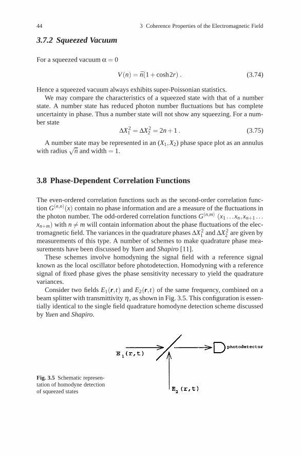
44 3 Coherence Properties of the Electromagnetic Field
3.7.2 Squeezed Vacuum
For a squeezed vacuum α = 0
V (n) = n(1 + cosh2r) . (3.74)
Hence a squeezed vacuum always exhibits super-Poissonian statistics.We may compare the characteristics of a squeezed state with that of a number
state. A number state has reduced photon number fluctuations but has completeuncertainty in phase. Thus a number state will not show any squeezing. For a num-ber state
ΔX21 = ΔX2
2 = 2n + 1 . (3.75)
A number state may be represented in an (X1,X2) phase space plot as an annuluswith radius
√n and width = 1.
3.8 Phase-Dependent Correlation Functions
The even-ordered correlation functions such as the second-order correlation func-tion G(n,n)(x) contain no phase information and are a measure of the fluctuations inthe photon number. The odd-ordered correlation functions G(n,m) (x1 . . .xn,xn+1 . . .xn+m) with n �= m will contain information about the phase fluctuations of the elec-tromagnetic field. The variances in the quadrature phases ΔX2
1 and ΔX22 are given by
measurements of this type. A number of schemes to make quadrature phase mea-surements have been discussed by Yuen and Shapiro [11].
These schemes involve homodyning the signal field with a reference signalknown as the local oscillator before photodetection. Homodyning with a referencesignal of fixed phase gives the phase sensitivity necessary to yield the quadraturevariances.
Consider two fields E1(r,t) and E2(r,t) of the same frequency, combined on abeam splitter with transmittivity η , as shown in Fig. 3.5. This configuration is essen-tially identical to the single field quadrature homodyne detection scheme discussedby Yuen and Shapiro.
Fig. 3.5 Schematic represen-tation of homodyne detectionof squeezed states
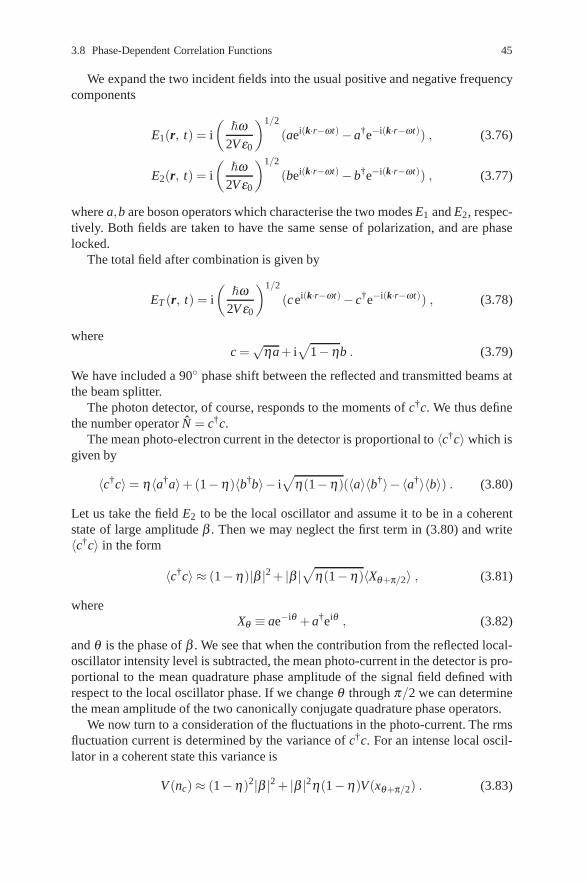
3.8 Phase-Dependent Correlation Functions 45
We expand the two incident fields into the usual positive and negative frequencycomponents
E1(r, t) = i
(�ω
2Vε0
)1/2
(aei(k·r−ωt)−a†e−i(k·r−ωt)) , (3.76)
E2(r, t) = i
(�ω
2Vε0
)1/2
(bei(k·r−ωt)−b†e−i(k·r−ωt)) , (3.77)
where a,b are boson operators which characterise the two modes E1 and E2, respec-tively. Both fields are taken to have the same sense of polarization, and are phaselocked.
The total field after combination is given by
ET (r, t) = i
(�ω
2Vε0
)1/2
(cei(k·r−ωt)− c†e−i(k·r−ωt)) , (3.78)
wherec =√
ηa+ i√
1−ηb . (3.79)
We have included a 90◦ phase shift between the reflected and transmitted beams atthe beam splitter.
The photon detector, of course, responds to the moments of c†c. We thus definethe number operator N = c†c.
The mean photo-electron current in the detector is proportional to 〈c†c〉 which isgiven by
〈c†c〉= η〈a†a〉+(1−η)〈b†b〉− i√
η(1−η)(〈a〉〈b†〉− 〈a†〉〈b〉) . (3.80)
Let us take the field E2 to be the local oscillator and assume it to be in a coherentstate of large amplitude β . Then we may neglect the first term in (3.80) and write〈c†c〉 in the form
〈c†c〉 ≈ (1−η)|β |2 + |β |√
η(1−η)〈Xθ+π/2〉 , (3.81)
whereXθ ≡ ae−iθ + a†eiθ , (3.82)
and θ is the phase of β . We see that when the contribution from the reflected local-oscillator intensity level is subtracted, the mean photo-current in the detector is pro-portional to the mean quadrature phase amplitude of the signal field defined withrespect to the local oscillator phase. If we change θ through π/2 we can determinethe mean amplitude of the two canonically conjugate quadrature phase operators.
We now turn to a consideration of the fluctuations in the photo-current. The rmsfluctuation current is determined by the variance of c†c. For an intense local oscil-lator in a coherent state this variance is
V (nc)≈ (1−η)2|β |2 + |β |2η(1−η)V(xθ+π/2) . (3.83)

46 3 Coherence Properties of the Electromagnetic Field
The first term here represents reflected local oscillator intensity fluctuations. If thisterm is subtracted out, the photo-current fluctuations are determined by the variancesin Xθ+π/2, the measured quadrature phase operator. To subtract out the contributionof the reflected local oscillator field balanced homodyne detection may be used. Inthis scheme the output from both ports of the beam splitter is directed to a pho-todetector and the resulting currents combined with appropriate phase shifts beforesubsequent analysis. Balanced homodyne detection realises a direct measurementof the signal field quadrature phase operators [11]. Alternatively, the contributionfrom the local oscillator intensity fluctuations may be reduced by making the trans-mittivity η ≈ 1, in which case the dominant contribution to V (nc) comes from thesecond term in (3.83).
3.9 Photon Counting Measurements
3.9.1 Classical Theory
Consider radiation of intensity I(t) falling on a photo-electric counter. The proba-bility that a count occurs in a time dt is given by
Δp(t) = αI(t)dt . (3.84)
The parameter α is a measure of the sensitivity of the detector, and depends on thearea of the detector and the spectral range of the incident light. Suppose initiallythere are no random fluctuations in the intensity I(t). Now 1−Δp(t ′) represents theprobability that no counts occur in the time interval dt ′ at t ′. Then assuming theindependence of photocounts in different time intervals the joint probability that nocounts occur in an entire interval t to t + T is given by the product
t+T
∏t
[1−Δp(t ′)]≈t+T
∏t
exp[−Δp(t ′)]
= exp
[−
t+T
∑t
Δp(t ′)
]
= exp
⎡⎣−
t+T∫t
dp(t ′)
⎤⎦ . (3.85)
Thus the probability for no counts in the interval t to t + T is
P0(T + t,t) = exp
⎡⎣−α
t+T∫t
I(t ′)dt ′⎤⎦ . (3.86)

3.9 Photon Counting Measurements 47
The probability P1(T + t,t) that one count occurs between t and t + T is
∑t′′
dp(t ′′)t+T
∏t
[1−Δp(t ′)]→t+T∫t
dp(t ′′)exp
⎡⎣−
t+T∫t
dp(t ′)
⎤⎦ . (3.87)
Hence
P1(T + t, t) =
⎡⎣α
t+T∫t
I(t ′)dt ′⎤⎦exp
[−α
∫ t+T
tI(t ′)dt ′
]. (3.88)
Following this reasoning the probability for n counts in the interval t to t + T is
Pn(t, T ) =1n!
[αT I(t, T )]n exp[−αT I(t, T )] , (3.89)
where
I(t, T ) =1T
t+T∫t
I(t ′)dt ′
is the mean intensity during the counting interval.Now since I(t,T ) may vary from one counting interval to the next, Pn(T ) is a
time average of Pn(t,T ) over a large number of different starting times
Pn(T ) = 〈Pn(t,T )〉
=⟨
[αI(t, T )T ]n
n!exp[−αI(t, T )T ]
⟩. (3.90)
This formula was first derived by Mandel [12].We note a useful generating function for the photon-counting distribution is
Q(λ , T ) =∞
∑n=0
(1−λ )nPn(T ) . (3.91)
The factorial moments of the photon counting distribution may be obtained asfollows:
n(n−1) . . .(n− k) =∞
∑n=0
n(n−1) . . .(n− k)Pn(T )
= (−1)k ∂ k
∂λ k Q(λ , T )∣∣∣∣λ=0
. (3.92)
We shall now consider some important cases of the photon counting formula (3.89).

48 3 Coherence Properties of the Electromagnetic Field
3.9.2 Constant Intensity
In the simplest case of a constant intensity I(t,T ) is independent of t and T , hence
I(t, T ) = I . (3.93)
In this case the averaging over a fluctuating intensity I(t) is unnecessary and
Pn(T ) =nn
n!exp(−n) , (3.94)
wheren = αIT .
This is a Poisson distribution for which the variance V (n) = n.
3.9.3 Fluctuating Intensity–Short-Time Limit
When the intensity is fluctuating, (3.89) can be simplified in the limit where thecounting time T is short compared to the coherence time τc over which the intensitychanges. If, during the interval T, I(t) remains reasonably constant then
I(t,T ) = I(t) . (3.95)
With ergodic hypothesis for a stationary light source we may convert the timeaverage in (3.90) into an ensemble average over the distribution p(I(t)).
The photon counting formula may then be written
Pn(T ) =∞∫
0
[αI(t)T ]n
n!e−αI(t)T p(I(t))dI(t) . (3.96)
In the following we replace I(t) by the stochastic variable I for ease of notation.The mean photon count is
n =∞
∑n=0
nPn(T ) =∞∫
0
∞
∑n=0
n(αIT )n
n!e−αIT p(I)dI
=∞∫
0
αT Ip(I)dI = αT 〈I〉 . (3.97)
Defining moments of intensity as
〈In〉=∞∫
0
In p(I)dI , (3.98)

3.9 Photon Counting Measurements 49
we find for the mean square count
n2 =∞
∑n=0
n2Pn(T ) =∞∫
0
(α2T 2I2 + αT I)p(I)dI
= α2T 2〈I2〉+ αT 〈I〉 . (3.99)
Thus the variance is
V (n) = n2− n2 = αT 〈I〉+ α2T 2(〈I2〉− 〈I〉2) . (3.100)
We note that this is always greater than the mean unless p(I) is a Dirac delta functionδ (I− I0). This is true for classical fields. For certain quantum mechanical fields weshall see that it is possible to obtain V (n) < n.
A thermal light field has the following probability distribution for its intensity
p(I) =1I0
exp
(−II0
), (3.101)
with moments〈In〉= n!In
0 .
The mean and variance of the photocount distribution are
n = αTI0, V (n) = n(1 + n) . (3.102)
The photon-counting distribution is
Pn(T ) =(αT )n
I0n!
∞∫0
In exp
[−I
(αT +
1I0
)]dI
=(αT )n
I0n!
(αT +
1I0
)−(n+1) ∞∫0
xne−xdx n!
=1
(1 + n)
(n
1 + n
)n
. (3.103)
This power-law distribution for thermal light has been verified in photon-countingexperiments. Experiments have also shown that the photon count distribution ofhighly stabilized lasers is approximated by a Poisson distribution [8, 13].
We conclude with a comment on the form assumed by I(t,T ) if the depletion ofthe signal field by the detection process is taken into account. Then
I(t) = I0e−λ t , (3.104)
where λ is the rate of photon absorption. Then

50 3 Coherence Properties of the Electromagnetic Field
I(t, T ) =I0
T
t+T∫t
e−λ t′ dt ′ , (3.105)
Thus
I(τ, T ) =I(t)λ T
(1− e−λ T) . (3.106)
We note that for short counting times this has the same form as (3.95).
3.10 Quantum Mechanical Photon Count Distribution
The photon count distribution for a quantum mechanical field may be written in aformally similar way to the classical expression [14]
Pn(T ) =⟨
:[αI(T )T ]n
n!exp[−αI(T )T ] :
⟩(3.107)
where
I(T ) =1T
T∫0
I(t)dt
=1T
T∫0
E(−)(r, t)E(+)(r, t) dt (3.108)
and : : denotes normal ordering of the operators. We shall demonstrate the use ofthis formula for a single-mode field, in which case (3.107) may be written as
Pn(T ) = Tr
(ρ :
[μ(T )a†a]n
n!exp[−a†aμ(T )] :
)(3.109)
where μ(T ) is the probability for detecting one photon in time T from a one photonfield. The explicit form of μ(T ) depends on the physical situation, e.g., μ(T ) = λ Tfor an open system and μ(T ) = (1− e−λ T) for a closed system.
The photon count distribution may be related to the diagonal matrix elementsPn = 〈n|ρ |n〉 of ρ by
Pm(T ) = ∑n
Pn[μ(T )]m
m!
⟨n
∣∣∣∣∣∞
∑l=0
μ(T )l
l!a†m+lam+l
∣∣∣∣∣n⟩
. (3.110)
This gives
Pm(T ) =∞
∑n=m
Pn
n−m
∑l=0
(−1)l μ(T )l
l!n!
(n−m− l)!. (3.111)

3.10 Quantum Mechanical Photon Count Distribution 51
The l summation is equivalent to a binomial expansion and we may write [15]
Pm(T ) =∞
∑n=m
Pn
(nm
)[μ(T )]m[1− μ(T)]n−m (3.112)
where (nm
)=
n!m!(n−m)!
.
This distribution is known as the Bernoulli distribution.The photo-count distribution Pn(T ) is only the same as Pn in the case of unit
quantum efficiencyPm(T ) = Pm, μ(T ) = 1 . (3.113)
In practice, quantum efficiencies are less than unity and the photon-count distri-bution is only indirectly related to Pn.
The following results may be proved:
3.10.1 Coherent Light
Pn =nn
n!exp(−n) , (3.114)
Pm(T ) =[μ(T )n]m
m!exp[−μ(T )n] . (3.115)
3.10.2 Chaotic Light
Pn =(n)n
(1 + n)1+n , (3.116)
Pm(T ) =[μ(T )n]m
[1 + μ(T)n]1+m . (3.117)
These results agree with those obtained by semiclassical methods, see (3.94 and3.103). In these cases Pn and Pm(T ) have the same mathematical form with themean number m of counted photons related to the mean number n of photons in themode by m = μ(T )n. No such simple relation holds in general.
For example, for a photon number state, Pn is a delta function δnn0 but the photo-count distribution Pm(T ) is non zero for all m≤ n0. However the normalized secondorder factorial moments are the same in all cases.
For a single-mode field
∑m(m−1)Pm(T )
m2 = ∑n
(n−1)Pn
n2 = g(2)(0) . (3.118)

52 3 Coherence Properties of the Electromagnetic Field
Thus the second-order correlation function g(2)(0) is directly obtainable from thephoto-count distribution without any dependence on the quantum efficiency μ(T ).For a multimode field a more complicated relation holds.
3.10.3 Photo-Electron Current Fluctuations
We now consider how the photon number statistics determines the statistics of theobserved photo-electron current. Each individual photon detection produces a smallcurrent pulse, the observed current over a counting interval from t−T to t is thendue to the accumulated electrical pulses over this interval. Thus we write
i(t) =t∫
t−T
F(t ′)dn(t ′) . (3.119)
Here F(t ′) is a response function which determines the current resulting from eachphoton detection event. We assume F(t ′) is flat, i.e. independent of t,
F(t ′) =GeT
, (3.120)
where e is the electronic charge and G is a gain factor. Then the photo-electroncurrent is given by
i(t) =GeT
n , (3.121)
where n is the total number of photon detection events over the counting interval.The mean current is then given by
i(t) =GeT
∞
∑n=0
nPn(T ; t) , (3.122)
where Pn(T,t) is given by (3.89) with
I(t, T ) =1T
t∫t−T
dt ′ E(−)(t ′)E(+)(t ′) . (3.123)
Thusi(t) = (αGe)〈: I(t, T ) :〉 . (3.124)
The current power spectrum is directly related to the statistical properties of thecurrent by
S(ω) =1π
∞∫0
dτ cos (ωt) i(0)i(τ) . (3.125)

3.10 Quantum Mechanical Photon Count Distribution 53
The two-time correlation function is determined by joint emission probabilities forphoto-electrons which are generalisations of the single photon result in (3.84). Ex-plicit expressions were given by Carmichael [16]. The result is, with the definitionsof (3.120).
i(0)i(τ) = (αGe)2[〈: I(T, 0)I(T, τ) :〉+ θ (T − τ)〈: I(τ−T, 0) :〉] (3.126)
where θ (x) is zero for x ≤ 0 and unity otherwise. For multiple time correlations:: also signifies time ordering (time arguments increasing to the left in products ofannihilation operators). In the case of constant intensity
i(0)i(τ) =(αζ Ge)2[〈a†(0)a†(τ)a(τ)a(0)〉]
+ (Ge)2αζ[
θ (T − τ)(T − τ)
T 2 〈a†(0)a(0)〉]
(3.127)
where ζ is a scale factor that converts the intensity operator into a photon-flux op-erator. For plane waves it is given by
ζ =ε0 cA�ωc
(3.128)
where A is the transverse area of the field over which the field is measured, and ωc
the frequency of the field. Using the following result for the delta function
∞∫0
dt ′ f (t ′)δ (t ′) =12
f (0) , (3.129)
one may show that
limT→0
θ (T − t)T 2 (T − t) = δ (t) . (3.130)
Then in the limit of broad-band detector response (T → 0)
i(0)i(τ) = (αGeζ )2〈a†(0)a†(τ)a(τ)a(0)〉+ αζ (Ge)2〈a†(0)a(0)〉δ(τ) (3.131)
The last term in this expression is the shot noise contribution to the current.It is more convenient to write this expression directly in terms of the normally-
ordered correlation function
〈: I(0), I(τ) :〉 ≡ ζ 2[〈a†(0)a†(τ)a(τ)a(0)〉− 〈a†(0)a(0)〉2] . (3.132)
Then
i(0)i(τ) = (αGeζ )2〈a†(0)a(0)〉2 + αζ (Ge)2〈a†(0)a(0)〉δ(τ)
+ (αGe)2〈: I(0), I(τ) :〉 . (3.133)

54 3 Coherence Properties of the Electromagnetic Field
The first term is a DC term and does not contribute to the spectrum. The secondterm is the shot-noise contribution. The final term represents intensity fluctuations,which for a coherent field is zero.
Exercises
3.1 Calculate the mean intensity at the screen when the two slits of a Young’sinterference experiment are illuminated by the two photon state (b†)2|0〉/√2where b = (a1 +a2)/
√2 and ai is the annihilation operator for the mode radi-
ated by slit i.3.2 In balanced homodyne detection the measured photocurrent is determined by
the moments of the photon number difference at the two output ports of thebeam splitter. Show that the variance of the photon-number difference for a50/50 beam splitter is
V (n−) = |β |2V (Xθ+π/2)
where |β |2 is the intensity of the local oscillator. Thus the local oscillatorintensity fluctuations do not contribute.
3.3 Show that the probability to detect m photons with unit quantum efficiencyin a field which has been transmitted by a beam splitter of transmitivity μ , isgiven by
Pm(μ) =∞
∑n=m
Pn
(nm
)μm(1− μ)n−m
where Pn is the photon number distribution for the field before passing throughthe beam splitter.
3.4 A beam splitter transforms incoming mode operators ai, bi to the outgoingoperators a0, b0 where
a0 =√
ηai− i√
1−ηbi, b0 =√
ηbi− i√
1−ηai .
(a) Show that such a transformation may be generated by the unitary operator
T = exp[−iθ (a†b + ab†)], η = cos2 Θ .
(b) Thus show that if the incoming state is a coherent state |αi〉 ⊗ |βi〉, theoutgoing state is also a coherent state with
α0 =√
ηαi− i√
1−ηβi, β0 =√
ηβi− i√
1−ηαi .
(c) Show that, if the incoming state is the product number state |1〉⊗ |1〉, theoutgoing state is

Further Reading 55
(2η−1)|1〉|1〉+ i√
2η(1−η)(|2〉|0〉+ |0〉|2〉).
Note that when η = 1/2 the ‘coincidence’ term |1〉|1〉 does not appear, a resultknown as Hong-Ou-Mandel interference.
References
1. R.J. Glauber: Phys. Rev. 130, 2529 (1963)2. M. Born, E. Wolf: Principles of Optics, 3rd edn. (Pergamon, London 1965)3. P.A.M. Dirac: The Principles of Quantum Mechanics, 3rd edn. (Clarendon, London 1947)4. G.I. Taylor: Proc. Cam. Phil. Soc. Math. Phys. Sci. 15, 114 (1909)5. P. Grangier, G. Roger, A. Aspect: Europhys. Lett. 1, 173 (1986)6. R.F. Pfleegor, L. Mandel: Phys. Rev. 159, 1084 (1967)7. R. Hanbury-Brown, R.W. Twiss: Nature 177, 27 (1956)8. F.T. Arecchi, E. Gatti, A. Sona: Phys. Rev. Lett. 20, 27 (1966); F.T. Arecchi, Phys. Lett. 16,
32 (1966)9. W. Demtroeder: Laser Spectroscopy, 2nd edn. (Springer, Berlin, Heidelberg 1993)
10. L. Mandel: Phys. Rev. Lett. 49, 136 (1982)11. H.P. Yuen, J.H. Shapiro: IEEE Trans. IT 26, 78 (1980)12. L. Mandel: Progress in Optics 2, 183 (North-Holland, Amsterdam 1963)13. E.R. Pike: In Quantum Optics, ed. by R.J. Glauber (Academic, New York 1970)14. P.L. Kelley, W.H. Kleiner: Phys. Rev. 136, 316 (1964)15. M.O. Scully, W.E. Lamb: Phys. Rev. 179, 368 (1969)16. H.J. Carmichael: J. Opt. Soc. Am. B 4, 1588 (1987)17. D. Mettzer, L. Mandel: IEEE J. QE-6, 661 (1970)
Further Reading
Meystre, P., M. Sargent III: Elements of Quantum Optics, 2nd edn. (Springer, Berlin,Heidelberg 1991)
Perina, J.: Coherence of Light (van Nostrand Reinhold, London 1972)
Chapter 4Representations of the Electromagnetic Field
Abstract A full description of the electromagnetic field requires a quantumstatistical treatment. The electromagnetic field has an infinite number of modes andeach mode requires a statistical description in terms of its allowed quantum states.However, as the modes are described by independent Hilbert spaces, we may formthe statistical description of the entire field as the product of the distribution functionfor each mode. This enables us to confine our description to a single mode withoutloss of generality.
In this chapter we introduce a number of possible representations for the densityoperator of the electromagnetic field. One representation is to expand the densityoperator in terms of the number states. Alternatively the coherent states allow anumber of possible representations via the P function, the Wigner function and theQ function.
4.1 Expansion in Number States
The number or Fock states form a complete set, hence a general expansion of ρ is
ρ = ∑Cnm|n〉〈m| . (4.1)
The expansion coefficients Cnm are complex and there is an infinite number of them.This makes the general expansion rather less useful, particularly for problems wherethe phase-dependent properties of the electromagnetic field are important and hencethe full expansion is necessary. However, in certain cases where only the photonnumber distribution is of interest the reduced expansion
ρ = ∑Pn|n〉〈n| , (4.2)
may be used. Here Pn is a probability distribution giving the probability of havingn photons in the mode. This is not a general representation for all fields but mayprove useful for certain fields. For example, a chaotic field, which has no phaseinformation, has the distribution
57
58 4 Representations of the Electromagnetic Field
Pn =1
(1 + n)
(n
1 + n
)n
, (4.3)
where n is the mean number of photons. This is derived by maximising the entropy
S =−TR{ρ lnρ} , (4.4)
subject to the constraint Tr{ρa†a} = n, and is just the usual Planck distribution forblack-body radiation with
n =1
ehω/kT −1. (4.5)
The second-order correlation function g2(0) may be written according to (3.66)
g2(0) = 1 +V (n)− n
n2 , (4.6)
where V (n) is the variance of the distribution function Pn. Hence, for the power-lawdistribution V (n) = n2 + n we find g(2)(0) = 2. For a field with a Poisson distributionof photons
Pn =e−n
n!nn (4.7)
the variance V (n) = n, hence g(2)(0) = 1.A coherent state has a Poisson distribution of photons. However, a measurement
of g(2)(0) would not distinguish between a coherent state and a field prepared froman incoherent mixture with a Poisson distribution. In order to distinguish betweenthese two fields a phase-dependent measurement such as a measurement of ΔX1,ΔX2 would need to be made.
4.2 Expansion in Coherent States
4.2.1 P Representation
The coherent states |α〉 form a complete set of states, in fact, an overcomplete setof states. They may therefore be used as a basis set despite the fact that they arenon-orthogonal. The following diagonal representation in terms of coherent stateswas introduced independently by Glauber [1] and Sudarshan [2]
ρ =∫
P(α)|α〉〈α|d2α , (4.8)
where d2α = d(Re{α})d(Im{α}). It has found wide-spread application in quantumoptics.
Now it might be imagined that the function P(α) is analogous to a probabilitydistribution for the values of α . However, in general this is not the case since the

4.2 Expansion in Coherent States 59
projection operator |α〉〈α| is onto non-orthogonal states, and hence P(α) cannotbe interpreted as a genuine probability distribution. We may note that the coher-ent states |α〉 and |α ′〉 are approximately orthogonal for |α −α ′| � 1, see (2.41).Hence, if P(α) is slowly varying over such large ranges of the parameter there is anapproximate sense in which P(α) may be interpreted with a classical description.There are, however, certain quantum states of the radiation field where P(α) maytake on negative values or become highly singular. For these fields there is no clas-sical description and P(α) clearly cannot be interpreted as a classical probabilitydistribution. Let us now consider examples of fields which may be described by theP representation:
(i) Coherent state
Ifρ = |α0〉〈α0| , (4.9)
thenP(α) = δ (2)(α−α0) . (4.10)
(ii) Chaotic state
For a chaotic state it follows from the central limit theorem that P(α) is aGaussian
P(α) =1
πne−|α |
2/n . (4.11)
That this is equivalent to the result for Pn is clear if we take matrix elements
Pn = 〈n|ρ |n〉=∫
P(α)|〈n|α〉|2d2α =1
πn
∫e−|α |
2/n |α|2n
n!e−|α |
2d2α . (4.12)
Using the identity
π−1(l!m!)−1/2∫
exp(−C|α|2)α l(α∗)md2α = δlmC−(m+1) , (4.13)
which holds for C > 0 and choosing
C =1 + n
n
we find
Pn =1
1 + n
(n
1 + n
)n
. (4.14)
For a mixture of a coherent and a chaotic state the P function is
P(α) =1
πne−|α−α0|2/n , (4.15)
which may be derived using the following convolution property of P(α). Considera field produced by two independent sources. The first source acting constructsthe field

60 4 Representations of the Electromagnetic Field
ρ1 =∫
P1(α1)|α1〉〈α1|d2α1 . (4.16)
Acting alone the second source would produce the field
ρ2 =∫
P2(α2)|α2〉〈α2|d2α2 =∫
P2(α2)D(α2)|0〉〈0|D−1(α2)d2α2 . (4.17)
The second source acting after the first field generates the field
ρ =∫
P2(α2)D(α2)ρ1D−1(α2)d2α2
=∫
P2(α2)P1(α1)|α1 + α2〉〈α1 + α2|d2α1 d2α2 . (4.18)
The weight function P(α) for the superposed excitations is therefore
P(α) =∫
δ 2(α−α1−α2)P1(α1)P2(α2)d2α1 d2α2
=∫
P1(α−α ′)P2(α ′)d2α ′ . (4.19)
We see that the distribution function for the superposition of two fields is the con-volution of the distribution functions for each field.
a) Correlation Functions
The P(α) representation is convenient for evaluating normally-ordered products ofoperators, for example
〈a†nam〉=∫
P(α)α∗nαmd2α . (4.20)
This reduces the taking of quantum mechanical expectation values to a form similarto classical averaging.
Let us express the second-order correlation function in terms of P(α)
g(2)(0) = 1 +∫
P(α)[(|α|2)−〈|α|2〉]2 d2α[∫
P(α)|α|2 d2α]2. (4.21)
This looks functionally identical to the expression for classical fields. However, theargument that g(2)(0) must be greater than or equal to unity no longer holds sincefor certain fields as we have mentioned P(α) may take on negative values and allowfor a g(2)(0) < 1, that is, photon antibunching.
A similar result may be derived for the squeezing. We may write the variances inX1 and X2 as
ΔX21 = {1 +
∫P(α)[(α + α∗)− (〈α〉+ 〈α∗〉)]2 d2α},
ΔX22 =
{1 +
∫P(α)
[(α−α∗
i
)−(〈α〉− 〈α∗〉
i
)]2
d2α
}. (4.22)

4.2 Expansion in Coherent States 61
The condition for squeezing ΔX21 < 1, requires that P(α) takes on a negative value
along either the real or imaginary axis in the complex plane, but not both simulta-neously. Thus squeezing and antibunching are phenomena which are the exclusiveproperty of quantum fields and may not be generated by classical fields. Some am-biguity may arise in the case of squeezing which only has significance for quantumfields. If a classical field is assumed from the outset arbitrary squeezing may occurin either quadrature or both simultaneously.
Quantised fields for which P(α) is a positive function do not exhibit quantumproperties such as photon antibunching and squeezing. Such fields may be simulatedby a classical description which treats the complex field amplitude ε as a stochasticrandom variable with the probability distribution P(ε) and hence may be consideredas quasiclassical. Coherent and chaotic fields are familiar examples of fields with apositive P representation. Quantum fields exhibiting antibunching and/or squeezingcannot be described in classical terms. For such fields the P representation may benegative and highly singular. The coherent state has a P representation which is adelta function, defining the boundary between quantum and classical behaviour. Forfields exhibiting quantum behaviour such as a number state |n〉 or squeezed state|α,ε〉 no representation for P(α) in terms of tempered distributions exists. Thoughrepresentations in terms of generalised functions do exist [3], such representationsare highly singular, for example, derivatives of delta functions. We shall thereforelook for alternative representations to describe such quantum fields.
b) Covariance Matrix
Gaussian processes which arise, for example, in linearized fluctuation theory maybe characterized by a covariance matrix. A covariance matrix may be defined by
C(a,a†) =( 〈a2〉− 〈a〉2 1
2〈aa† + a†a〉− 〈a†〉〈a〉12 〈aa† + a†a〉− 〈a†〉〈a〉 〈a†2〉− 〈a†〉2
). (4.23)
One may also introduce a correlation matrix C(X1, X2) for the quadrature phaseoperators X1 and X2:
C(X1,X2)p,q =12〈XpXq + XqXp〉− 〈Xp〉〈Xq〉 (p,q = 1,2) . (4.24)
These two correlation matrices are related by
C(X1,X2) = ΩC(a,a†)ΩT (4.25)
where
Ω =(
1 1−i i
).
The covariance matrix Cp(α, α∗) defined by the moments of α and α∗ overP(α, α∗) is related to the covariance matrix C(a, a†) by
C(a,a†) = Cp(α,α∗)+12
(0 11 0
). (4.26)

62 4 Representations of the Electromagnetic Field
The distribution can be written in terms of the real variables
x1 = α + α∗, x2 =1i(α−α∗)
for which the covariance matrix relation is
C(X1,X2) = Cp(x1,x2)+ I . (4.27)
c) Characteristic Function
In practice, it proves useful to evaluate the P function through a characteristicfunction.
The density operator ρ is uniquely determined by its characteristic function
χ(η) = Tr{ρeηa†−η∗a} .
We may also define normally and antinormally ordered characteristic functions
χN(η) = Tr{ρeηa†e−η∗a} , (4.28)
χA(η) = Tr{ρe−η∗aeηa†} . (4.29)
Using the relation (2.25) the characteristic functions are related by
χ(η) = χN(η)exp
(−1
2|η |2
). (4.30)
If the density operator ρ has a P representation, then χN(η) is given by
χN(η) =∫〈α|eηa†
e−η∗a|α〉P(α)d2α =∫
eηα∗−η∗α P(α)d2α . (4.31)
Writing η and α in terms of their real and imaginary parts we find that (4.31) ex-presses χN(η) as a two-dimensional Fourier transform of P(α). The solution forP(α) is the inverse Fourier transform
P(α) =1π2
∫eαη∗−α∗η χN(η)d2η . (4.32)
Thus the criterion for the existence of a P representation is the existence of a Fouriertransform for the normally-ordered characteristic function χN(η).
4.2.2 Wigner’s Phase-Space Density
The first quasi-probability distribution was introduced into quantum mechanics byWigner [4]. The Wigner function may be defined as the Fourier transform of thesymmetrically ordered characteristic function χ(η)

4.2 Expansion in Coherent States 63
W (α) =1π2
∫exp(η∗α−ηα∗)χ(η)d2η . (4.33)
The Wigner distribution always exists but is not necessarily positive.The relationship between the Wigner distribution and the P(α) distribution may
be obtained via the characteristic functions. Using (4.30) we may express the Wignerfunction as
W (α) =1π2
∫exp(η∗α−ηα∗)χN(η)e−1/2|η|2d2η
=1π2
∫Tr{ρeη(a†−α∗)e−η∗(a−α)}e−1/2|η|2d2η
=1π2
∫P(β )exp[η(β ∗ −α∗)−η∗(β −α)− 1
2|η |2]d2η d2β . (4.34)
Substituting ε = η/√
2 leads to
W (α) =2π2
∫P(β )exp[
√2ε(β ∗ −α∗)−
√2ε∗(β −α)−|ε|2]d2ε d2β . (4.35)
The integral may be evaluated using the identity
1π
∫d2η exp(−λ |η |2 + μη + νη∗) =
1λ
exp(μν
λ
)(4.36)
which holds for Re{λ}> 0 and arbitrary μ , ν . This gives
W (α) =2π
∫P(β )exp(−2|β −α|2)d2β . (4.37)
That is, the Wigner function is a Gaussian convolution of the P function.The covariance matrix Cw(α, α∗) defined by the moments of α and α∗ over
W (α, α∗) is related to the covariance matrix C(a, a†) defined by (4.23) by
C(a,a†) = Cw(α,α∗) . (4.38)
The error areas discussed in Chap. 2 may rigorously be derived as contours ofthe Wigner function. We shall now study the Wigner functions for several states ofthis radiation field and their corresponding contours.
As it is defined in (4.33) the Wigner function is normalised as∫d2αW (α) = 1 (4.39)
We have defined the quadrature phase operators Xi as (2.56)
a =12(X1 + iX2) (4.40)
If we denote the eigenstates of Xi as |xi〉, we can write the Wigner function as afunction of xi using
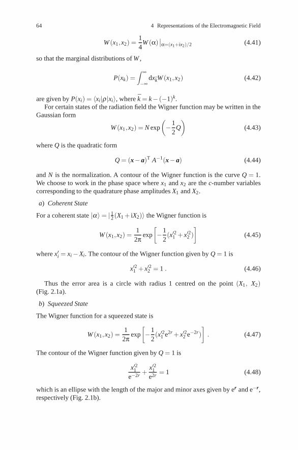
64 4 Representations of the Electromagnetic Field
W (x1,x2) =14
W (α)∣∣α=(x1+ix2)/2 (4.41)
so that the marginal distributions of W ,
P(xk) =∫ ∞
−∞dxkW (x1,x2) (4.42)
are given by P(xi) = 〈xi|ρ |xi〉, where k = k− (−1)k.For certain states of the radiation field the Wigner function may be written in the
Gaussian form
W (x1,x2) = N exp
(−1
2Q
)(4.43)
where Q is the quadratic form
Q = (x−a)T A−1(x−a) (4.44)
and N is the normalization. A contour of the Wigner function is the curve Q = 1.We choose to work in the phase space where x1 and x2 are the c-number variablescorresponding to the quadrature phase amplitudes X1 and X2.
a) Coherent State
For a coherent state |α〉= | 12 (X1 + iX2)〉 the Wigner function is
W (x1,x2) =1
2πexp
[−1
2(x′21 + x′22 )
](4.45)
where x′i = xi−Xi. The contour of the Wigner function given by Q = 1 is
x′21 + x′22 = 1 . (4.46)
Thus the error area is a circle with radius 1 centred on the point (X1, X2)(Fig. 2.1a).
b) Squeezed State
The Wigner function for a squeezed state is
W (x1,x2) =1
2πexp
[−1
2(x′21 e2r + x′22 e−2r)
]. (4.47)
The contour of the Wigner function given by Q = 1 is
x′21e−2r +
x′21e2r = 1 (4.48)
which is an ellipse with the length of the major and minor axes given by er and e−r,respectively (Fig. 2.1b).

4.2 Expansion in Coherent States 65
c) Number State
The Wigner function for a number state |n〉 is
W (x1,x2) =2π
(−1)nLn(4r2)e−2r2(4.49)
where r2 = x21 + x2
2, and Ln(x) is the Laguerre polynomial. This Wigner function isclearly negative.
The Wigner function gives direct symmetrically-ordered moments such as thosearising in the calculation of the variances of quadrature phases.
4.2.3 Q Function
An alternative function is the diagonal matrix elements of the density operator in apure coherent state
Q(α) =〈α|ρ |α〉
π≥ 0 . (4.50)
This is clearly a non-negative function since the density operator is a positive oper-ator. It is also a bounded function
Q(α) <1π
.
Writing the distribution in terms of the real variables
x1 = α + α∗, x2 =−i(α−α∗)
the covariance matrix relation is
C(X1,X2) = CQ(x1,x2)− I .
The Q function may be expressed as the Fourier transform of the antinormally-ordered characteristic function χA(η)
χA(η) = Tr{ρe−η∗aeηa†}=∫
d2απ〈α|eηa†
ρe−η∗a|α〉=∫
eηα∗−η∗α Q(α)d2α .
(4.51)Thus Q(α) is the inverse Fourier transform
Q(α) =1π2
∫eαη∗−α∗η χA(η)d2η . (4.52)
The relation between the P(α) and the Q(α) follows from
Q(α) =〈α|ρ |α〉
π=
1π
∫P(β )|〈α|β 〉|2d2β =
1π
∫P(β )e−|α−β |2d2β . (4.53)

66 4 Representations of the Electromagnetic Field
That is, the Q function like the Wigner function is a Gaussian convolution of the Pfunction. However, it is convoluted with a Gaussian which has
√2 times the width
of the Wigner function which accounts for the rather more well-behaved properties.The Q function is convenient for evaluating anti-normally-ordered moments
〈ana†m〉=∫
αnα∗mQ(α,α∗)d2α . (4.54)
The covariance matrix CQ(α, α∗) defined by the moments of α and α∗ overQ(α, α∗) is related to the covariance matrix C(a, a†) defined by (4.23) by
C(a,a†) = CQ(α,α∗)− 12
(0 11 0
). (4.55)
The Q function has the advantage of existing for states where no P function ex-ists and unlike the Wigner or P function is always positive. The Q functions for acoherent state and a number state are easily obtained.
For a coherent state |β 〉 the Q function is
Q(α) =|〈α|β 〉|2
π=
e−|α−β |2
π. (4.56)
For a number state |n〉 the Q function is
Q(α) =|〈α|n〉|2
π=|α|2ne−|α |2
πn!. (4.57)
The Q function for a squeezed state |α, r〉 is defined as
Q(β ,β ∗) =1π|〈β |D(α)S(r)|0〉|2 . (4.58)
This is a multivariate Gaussian distribution and may be written in terms of thequadrature phase variables x1 and x2 as
Q(x1,x2) =1
4π2 coshrexp
[−1
2(x−x0)TC−1(x−x0)
](4.59)
where
x0 = 2(Re{α}, Im{α}),x = (x1,x2),
C =(
e−2r + 1 00 e2r + 1
).
The Q function for a squeezed state is shown in Fig. 4.1.

4.2 Expansion in Coherent States 67
Fig. 4.1 Q function for a squeezed state with coherent amplitude α = 2.0, r = 1.0
4.2.4 R Representation
Any density operator ρ may be represented in a unique way by means of a functionof two complex variables R(α∗, β ) which is analytic throughout the finite α∗ andβ planes. The function R is given explicitly as
R(α∗,β ) = 〈α|ρ |β )exp[(|α|2 + |β |2)/2] . (4.60)
We may express the density operator in terms of R(α∗, β )
ρ =1π2
∫|α〉R(α∗,β )〈β |e−(|α |2+|β |2)/2d2α d2β . (4.61)
The normalization conditionTr{ρ}= 1
implies ∫〈γ|α〉〈α|ρ |β 〉〈β |γ〉d
2απ
d2βπ
d2γπ
= 1 . (4.62)
Interchanging the scalar products and performing the integrations over β and γ wearrive at the result
1π
∫〈α|ρ |α〉d2α = 1 (4.63)
which gives the normalization condition on R
1π
∫R(α∗,α)e−|α |
2d2α = 1 . (4.64)
The function R(α∗, β ) is analytic in α∗ and β (and therefore non-singular) andis by definition non-positive. It has a normalization that includes a Gaussian weightfactor. For these reasons it cannot have a Fokker–Planck equation or any direct in-terpretation as a quasiprobability. Nevertheless, the existence of this representationdoes demonstrate that a calculation of normally-ordered observables for any ρ ispossible with a non-singular representation.

68 4 Representations of the Electromagnetic Field
4.2.5 Generalized P Representations
Another representation which like the R representation uses an expansion in non-diagonal coherent state projection operators was suggested by Drummond andGardiner [5]. The representation is defined as follows
ρ =∫D
Λ(α,β )P(α,β )dμ(α,β ) (4.65)
where
Λ(α,β ) =|α〉〈β ∗|〈β ∗|α〉
and dμ(α, β ) is the integration measure which may be chosen to define differentclasses of possible representations and D is the domain of integration. The projectionoperator Λ(α, β ) is analytic in α and β . It is clear that the normalization conditionon ρ leads to the following normalization condition on P(α, β )
∫D
P(α,β )dμ(α,β ) = 1 . (4.66)
Thus, the P(α, β ) is normalisable and we shall see in Chap. 6 that it gives rise toFokker–Planck equations. The definition given by (4.65) leads to different represen-tations depending on the integration measure.
Useful choices of integration measure are
1. Glauber–Sudarshan P Representation
dμ(α,β ) = δ 2(α∗ −β )d2α d2β . (4.67)
This measure corresponds to the diagonal Glauber–Sudarshan P representation de-fined in (4.8).
2. Complex P Representation
dμ(α,β ) = dα dβ . (4.68)
Here (α, β ) are treated as complex variables which are to be integrated on individ-ual contours C, C′. The conditions for the existence of this representation are dis-cussed in the appendix. This particular representation may take on complex valuesso in no sense can it have any physical interpretation as a probability distribution.However, as we shall see it is an extremely useful representation giving exact resultsfor certain problems and physical observables such as all the single time correlationfunctions.
We shall now give some examples of the complex P representation.
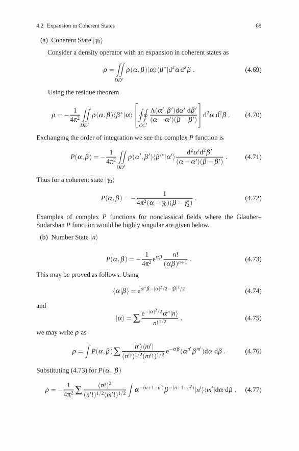
4.2 Expansion in Coherent States 69
(a) Coherent State |γ0〉Consider a density operator with an expansion in coherent states as
ρ =∫∫
DD′ρ(α,β )|α〉〈β ∗|d2α d2β . (4.69)
Using the residue theorem
ρ =− 14π2
∫∫
DD′ρ(α,β )〈β ∗|α〉
⎡⎣∮ ∮
CC′
Λ(α ′,β ′)dα ′ dβ ′
(α−α ′)(β −β ′)
⎤⎦d2α d2β . (4.70)
Exchanging the order of integration we see the complex P function is
P(α,β ) =− 14π2
∫∫
DD′ρ(α ′,β ′)〈β ′∗|α ′〉 d2α ′d2β ′
(α−α ′)(β −β ′). (4.71)
Thus for a coherent state |γ0〉
P(α,β ) =− 14π2(α− γ0)(β − γ∗0)
. (4.72)
Examples of complex P functions for nonclassical fields where the Glauber–Sudarshan P function would be highly singular are given below.
(b) Number State |n〉
P(α,β ) =− 14π2 eαβ n!
(αβ )n+1 . (4.73)
This may be proved as follows. Using
〈α|β 〉= eα∗β−|α |2/2−|β |2/2 (4.74)
and
|α〉= ∑ e−|α |2/2αn|n〉n!1/2
, (4.75)
we may write ρ as
ρ =∫
P(α,β )∑ |n′〉〈m′|(n′!)1/2(m′!)1/2
e−αβ (αn′β m′)dα dβ . (4.76)
Substituting (4.73) for P(α, β )
ρ =− 14π2 ∑ (n!)2
(n′!)1/2(m′!)1/2
∫α−(n+1−n′)β−(n+1−m′)|n′〉〈m′|dα dβ . (4.77)

70 4 Representations of the Electromagnetic Field
Choosing any contour of integration encircling the origin and using Cauchy’stheorem
12πi
∮dz zn = 0 if n≥ 0,
= 1 if n =−1,
= 0 if n <−1 . (4.78)
We findρ = |n〉〈n| .
(c) Squeezed State |γ, r〉The complex P representation for a squeezed state is
P(α,β ) = N exp{(α− γ)(β − γ∗)+ cothr[(α − γ)2 +(β − γ∗)2]} . (4.79)
This may be normalized by integrating along the imaginary axis for r real. Theresulting normalization for this choice of contour is
N =− 12πsinhr
.
As an example of the use of the complex P representation we shall consider thephoton counting formula given by (3.107). Using the diagonal coherent-state repre-sentation for ρ we may write the photon counting probability Pm(T ) as
Pm(T ) =∫
d2zP(z)(|z|2μ(T ))m
m!exp[−|z|2μ(T )] . (4.80)
An appealing feature of this equation is that Pm(T ) is given by an averaged Poissondistribution with P(z) in the role of a probability distribution over the complex fieldamplitude. It is a close analogue of the classical expression (3.96). We know how-ever that P(z) is not a true probability distribution and may take on negative values,and this may cause some anxiety over the validity of (4.80). In such cases we mayconsider a simple generalization of (4.80) by using the complex P representation forρ . The photocount probability is then given by
Pm(T ) =∫
CC′dz dz′ P(z,z′)
(zz′μ(T ))m
m!exp[−zz′μ(T )] . (4.81)
We shall demonstrate the use of this formula to calculate Pm(T ) for states for whichno well behaved diagonal P distribution exists.
a) Number State
For a number state with density operator ρ = |n〉〈n| we have
P(z,z′) =− 14π2 exp(zz′)n!(zz′)−n−1 (4.82)

4.2 Expansion in Coherent States 71
and the contours C and C′ enclose the origin. Substituting (4.81) for m > n theintegrand contains no poles and Pm(T ) = 0, while for m < n poles of order n−m+1contribute in each integration and we obtain the result of (3.112)
Pm(T ) =∞
∑n=m
(nm
)[μ(T )]m[1− μ(T)]n−m . (4.83)
b) Squeezed State
For a squeezed state with density operator ρ = |γ, r〉〈γ, r| where γ and r are takento be real, we have
P(z,z′) =− 12π
(sinhr)−1 exp{(z− γ)(z′ − γ)+ cothr[(z− γ)2
+(z′ − γ)2]} (4.84)
and the contours C and C′ are along the imaginary axes in z and z′ space, respec-tively. Performing the integration in (4.81) gives the formula, see (3.112),
Pm(T ) =∞
∑n=m
(nm
)[μ(T )]m[1− μ(T)]n−mPn (4.85)
with
Pn = (n! coshr)−1 exp[−γ2e2r(1 + tanhr)](tanhr)nH2n
(γer
√sinh2r
)
where the Hn(x) are Hermite polynomials. This agrees with the result of a deriva-tion using the number state representation (3.109) when we recognise that Pn =|〈n|γ, r〉|2.
4.2.6 Positive P Representation
The integration measure is chosen as
dμ(α,β ) = d2α d2β . (4.86)
This representation allows α, β to vary independently over the whole complexplane. It was proved in [5] that P(α, β ) always exists for a physical density op-erator and can always be chosen positive. For this reason we call it the posi-tive P representation. P(α, β ) has all the mathematical properties of a genuineprobability. It may also have an interpretation as a probability distribution [6]. Itproves a most useful representation, in particular, for problems where the Fokker–Planck equation in other representations may have a non-positive definite diffu-sion matrix. It may be shown that provided any Fokker–Planck equation exists

72 4 Representations of the Electromagnetic Field
for the time development in the Glauber–Sudarshan representation, a correspondingFokker–Planck equation exists with a positive semidefinite diffusion coefficient forthe positive P representation.
Exercises
4.1 Show that if a field with the P representation Pi(α) is incident on a 50/50 beamsplitter the output field has a P representation given by P0(α) = 2Pi(
√2α).
4.2 Show that the Wigner function may be written, in terms of the matrix elementsof ρ in the eigenstates of X1, as
W (x1,x2) =1
2π
∫ ∞
−∞dx e−ixx2〈x1 + x|ρ|x1− x〉
where x1 = α+ α∗ and x2 =−i(α−α∗).4.3 The complex P representation for a number state |n〉 is
P(α,β ) =− 14π2 eαβ n!
(αβ )n+1 .
Show that〈a†a〉=
∮dα dβ αβ P(α, β ) = n .
4.4 Use the complex P representation for a squeezed state |γ, r〉 with γ and r bothreal, to show that the photon number distribution for such a state is
Pn = (n! coshr)−1 exp[−γ2e2r(1 + tanhr)](tanhr)nH2n
(γer
√sinh2r
).
References
1. R.J. Glauber: Phys. Rev. 131, 2766 (1963)2. E.C.G. Sudarshan: Phys. Rev. Lett. 10, 277 (1963)3. J.R. Klauder, E.C.G. Sudarshan: Fundamentals of Quantum Optics (Benjamin, New York
1968)4. E.P. Wigner: Phys. Rev. 40, 749 (1932)5. P.D. Drummond, C.W. Gardiner: J. Phys. A 13, 2353 (1980)6. S.L. Braunstein, C.M. Caves and G.J. Milburn: Phys. Rev. A 43, 1153 (1991)

Chapter 5Quantum Phenomena in Simple Systemsin Nonlinear Optics
Abstract In this chapter we will analyse some simple processes in nonlinear opticswhere analytic solutions are possible. This will serve to illustrate how the formalismdeveloped in the preceding chapters may be applied. In addition, the simple exam-ples chosen illustrate many of the quantum phenomena studied in more complexsystems in later chapters.
This chapter will serve as an introduction to how quantum phenomena such asphoton antibunching, squeezing and violation of certain classical inequalities mayoccur in nonlinear optical systems. In addition, we include an introduction to quan-tum limits to amplification.
5.1 Single-Mode Quantum Statistics
A single-mode field is the simplest example of a quantum field. However, a num-ber of quantum features such as photon antibunching and squeezing may occur in asingle-mode field. To illustrate these phenomena we consider the degenerate para-metric amplifier which displays interesting quantum behaviour.
5.1.1 Degenerate Parametric Amplifier
One of the simplest interactions in nonlinear optics is where a photon of frequency2ω splits into two photons each with frequency ω . This process known as para-metric down conversion may occur in a medium with a second-order nonlinear sus-ceptibility χ (2). A detailed discussion on nonlinear optical interactions is left untilChap. 9.
We shall make use of the process of parametric down conversion to describe aparametric amplifier. In a parametric amplifier a signal at frequency ω is amplifiedby pumping a crystal with a χ (2) nonlinearity at frequency 2ω . We consider a simple
73

74 5 Quantum Phenomena in Simple Systems in Nonlinear Optics
model where the pump mode at frequency 2ω is classical and the signal mode atfrequency ω is described by the annihilation operator a. The Hamiltonian describingthe interaction is
H = �ωa†a− i�χ2
(a2e2iωt −a†2e−2iωt
), (5.1)
where χ is a constant proportional to the second-order nonlinear susceptibility andthe amplitude of the pump. If we work in the interaction picture we have the time-independent Hamiltonian
HI =−i�χ2
(a2−a†2) . (5.2)
The Heisenberg equations of motion are
dadt
=1i�
[a,HI] = χa†,da†
dt=
1i�
[a†,HI
]= χa . (5.3)
The interaction picture can be viewed equivalently as transforming to a frame rotat-ing at frequency ω .
These equations have the solution
a(t) = a(0)cosh χt + a† (0)sinh χt , (5.4)
which has the form of a generator of the squeezing transformation, see (2.60). Assuch we expect the light produced by parametric amplification to be squeezed. Thiscan immediately be seen by introducing the two quadrature phase amplitudes
X1 = a + a†, X2 =a−a†
i(5.5, 5.6)
which diagonalize (5.2 and 5.3)
dX1
dt= +χX1,
dX2
dt=−χX2. (5.7, 5.8)
These equations demonstrate that the parametric amplifier is a phase-sensitive am-plifier which amplifies one quadrature and attenuates the other:
X1 (t) = eχtX1 (0) , (5.9)
X2 (t) = e−χtX2 (0) . (5.10)
The parametric amplifier also reduces the noise in the X2 quadrature and increasesthe noise in the X1 quadrature. The variances V (Xi,t) satisfy the relations
V (X1,t) = e2χtV (X1,0) , (5.11)
V (X2,t) = e−2χtV (X2,0) . (5.12)

5.1 Single-Mode Quantum Statistics 75
For initial vacuum or coherent states V (Xi, 0) = 1, hence
V (X1,t) = e2χt ,
V (X2,t) = e−2χt , (5.13)
and the product of the variances satisfies the minimum uncertainty relation V (X1)V (X2) = 1. Thus the deamplified quadrature has less quantum noise than the vacuumlevel. The amount of squeezing or noise reduction is proportional to the strength ofthe nonlinearity, the amplitude of the pump and the interaction time.
5.1.2 Photon Statistics
We shall next consider the photon statistics of the light produced by the parametricamplifier. First we analyse the light produced from an initial vacuum state. Theintensity correlation function g(2)(0) in this case is
g(2) (0) =〈a† (t)a† (t)a(t)a(t)〉〈a† (t)a(t)〉2
= 1 +cosh2χt
sinh2 χt. (5.14)
This indicates that the squeezed light generated from an initial vacuum exhibitsphoton bunching (g(2)(0) > 1). This is expected for a squeezed vacuum which mustcontain correlated pairs of photons.
For an initial coherent state |α〉 we find the mean photon number
〈a† (t)a(t)〉= |α|2 (cosh2χt + cos2θ sinh2χt)+ sinh2 χt , (5.15)
where we have used α = |α|eiθ , and the intensity correlation function
g(2) (0)≈ 1 +1
|α|2 e−2χt
(e−2χt−1
), θ =
π4
, (5.16)
where |α|2 is large compared with sinh2 χt and sinh χt cosh χt.Thus under these conditions the photon statistics of the output light is anti-
bunched. We see that a parametric amplifier evolving from an initial coherent state|i|α|〉 evolves towards an amplitude squeezed state with a coherent amplitude of|α|e−χt . This reduction in amplitude is due to the dynamic contraction in the X2
direction described by (5.10) (Fig. 5.1).

76 5 Quantum Phenomena in Simple Systems in Nonlinear Optics
Fig. 5.1 Schematic represen-tation of the evolution of aninitial coherent state undergo-ing parametric amplification
5.1.3 Wigner Function
The full photon statistics of the light generated in parametric amplification may becalculated via a quasi-probability distribution. While we could choose to calculatethe P function we would find that it would become singular due to the quantumcorrelations which build up during the amplification process. Therefore we shallcalculate the Wigner distribution which is a nonsingular positive function for thisproblem.
The Wigner function describing the state of the parametric oscillator at any timet may now be calculated via the symmetrically ordered characteristic function,
χ (η ,t) = Tr{
ρ (0)eηa†(t)−η∗a(t)}
. (5.17)
Let us take the initial state to be the coherent state ρ(0) = |α0〉〈α0|. Then substitut-ing (5.4) into (5.17) we find
χ (η ,t) = exp
[ηα∗0 (t)−η∗α0 (t)− |η |
2
2cosh2χt + 1
4
(η2 + η∗2
)sinh2χt
],
(5.18)
whereα0 (t) = α0 cosh χt + α∗0 sinh χt . (5.19)
This may be written as
χ (η ,t) = exp[ηT ·α∗0 (t)+ 1
2 ηTΛη]
, (5.20)
ηT = (η ,−η∗) , (5.21)
αT0 (t) = (α0 (t) ,α∗0 (t)) (5.22)

5.2 Two-Mode Quantum Correlations 77
and
Λ =12
(sinh2χt cosh2χtcosh2χt sinh2χt
). (5.23)
The Wigner function is then given by the Fourier transform of χ(η , t), see (4.33).Using (4.36) the result is
W (α,t) =2π
exp
{12
[α−α0 (t)]T C−1α [α−α0 (t)]
}, (5.24)
where αT = (α, α∗). This is a two variable Gaussian with mean α0(t) and covari-ance matrix Cα = Λ. In terms of the real variables x1 = α + α∗. x2 = −i(α −α∗)(corresponding to the quadrature phase operators), the Wigner function becomes
W (x1,x2) =1
2πexp
{−1
2[x−x0 (t)]C−1
x [x−x0 (t)]}
, (5.25)
where
Cx =(
e2χt 00 e−2χt
). (5.26)
Thus the Wigner function is a two-dimensional Gaussian with the variance in fluctu-ations in the quadratures X1 and X2 given by the major and minor axes of the ellipticcontours.
5.2 Two-Mode Quantum Correlations
In two-mode systems there are a richer variety of quantum phenomena since thereexists the possibility of quantum correlations between the modes. These correlationsmay give rise to two mode squeezing such, as described by (2.85). There may alsoexist intensity and phase correlations between the modes. A simple system whichdisplays many of the above features is the non-degenerate parametric amplifier [1].
5.2.1 Non-degenerate Parametric Amplifier
The non-degenerate parametric amplifier is a simple generalization of the degen-erate parametric amplifier considered in the previous section. In this case the clas-sical pump mode at frequency 2ω1 interacts in a nonlinear optical medium withtwo modes at frequency ω1 and ω2. These frequencies sum to the pump frequency,2ω = ω1 + ω2. It is conventional to designate one mode as the signal and the otheras the idler.
The Hamiltonian describing this system is
H = �ω1a†1a1 +�ω2a†
2a2 + i�χ(
a†1a†
2e−2iωt −a1a2e2iωt)
, (5.27)
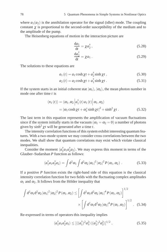
78 5 Quantum Phenomena in Simple Systems in Nonlinear Optics
where a1(a2) is the annihilation operator for the signal (idler) mode. The couplingconstant χ is proportional to the second-order susceptibility of the medium and tothe amplitude of the pump.
The Heisenberg equations of motion in the interaction picture are
da1
dt= χa†
2 , (5.28)
da†2
dt= χa1 . (5.29)
The solutions to these equations are
a1 (t) = a1 cosh χt + a†2 sinh χt , (5.30)
a2 (t) = a2 cosh χt + a†1 sinh χt . (5.31)
If the system starts in an initial coherent stat |α1〉, |α2〉, the mean photon number inmode one after time t is
〈n1 (t)〉= 〈α1,α2
∣∣∣a†1 (t)a1 (t)
∣∣∣α1,α2〉= |α1 cosh χt + α∗2 sinh χt|2 + sinh2 χt . (5.32)
The last term in this equation represents the amplification of vacuum fluctuationssince if the system initially starts in the vacuum (α1 = α2 = 0) a number of photonsgiven by sinh2 χt will be generated after a time t.
The intensity correlation functions of this system exhibit interesting quantum fea-tures. With a two-mode system we may consider cross correlations between the twomodes. We shall show that quantum correlations may exist which violate classicalinequalities.
Consider the moment 〈a†1a1a†
2a2〉. We may express this moment in terms of theGlauber–Sudarshan P function as follows:
〈a†1a1a†
2a2〉=∫
d2α1
∫d2α2 |α1|2 |α2|2 P(α1,α2) . (5.33)
If a positive P function exists the right-hand side of this equation is the classicalintensity correlation function for two fields with the fluctuating complex amplitudesα1 and α2. It follows from the Holder inequality that
∫d2α1d2α2 |α1|2 |α2|2 P(α1,α2)≤
[∫d2α1d2α2 |α1|4 P(α1,α2)
]1/2
×[∫
d2α1d2α2 |α2|4 P(α1,α2)]1/2
. (5.34)
Re-expressed in terms of operators this inequality implies
〈a†1a1a†
2a2〉 ≤ [〈(a†1)
2a21〉〈(a†
2)2a2
2〉]1/2 , (5.35)

5.2 Two-Mode Quantum Correlations 79
a result known as the Cauchy–Schwarz inequality. If the two modes are symmetricas for the non-degenerate parametric amplifier this inequality implies
〈a†1a1a†
2a2〉 ≤ 〈(a†1)
2a21〉 . (5.36)
Because we have assumed a positive P function this is a weak inequality and thereexists certain quantum fields which will violate it.
It is more usual to express the Cauchy–Schwarz inequality in terms of the second-order intensity correlation functions defined for a single-mode field in (3.63). Thetwo-mode intensity correlation function is defined by
g(2)12 (0) =
〈a†1a1a†
2a2〉〈a†
1a1〉〈a†2a2〉
. (5.37)
This definition together with
g(2)i (0) =
〈a†i a†
i aiai〉〈a†
i ai〉2(5.38)
enables one to write the Cauchy–Schwarz inequality as
[g(2)12 (0)]2 ≤ g(2)
1 (0)g(2)2 (0) . (5.39)
A stronger inequality may be derived for quantum fields when a Glauber–SudarshanP representation does not exist. The appropriate inequality for two non-commutingoperators is, see (3.26),
〈a†1a1a†
2a2〉2 ≤ 〈(a†1a1)2〉〈(a†
2a2)2〉 . (5.40)
For symmetrical systems this implies
〈a†1a1a†
2a2〉 ≤ 〈(a†1)
2a21〉+ 〈a†
1a1〉 (5.41)
or
g(2)12 (0)≤ g(2)
1 (0)+1
〈a†1a1〉
. (5.42)
We now show that the non-degenerate parametric amplifier if initially in theground state leads to a maximum violation of the Cauchy–Schwarz inequality(5.39), as is consistent with the inequality (5.42). That is, the correlations built upin the parametric amplifier are the maximum allowed by quantum mechanics.
In this system the following conservation law is easily seen to hold,
n1 (t)−n2 (t) = n1 (0)−n2 (0) , (5.43)
where ni(t)≡ a†i (t)ai(t). This conservation law has been exploited to give squeezing
in the photon number difference in a parametric amplifier as will be described in

80 5 Quantum Phenomena in Simple Systems in Nonlinear Optics
Chap. 8. Using this relation the intensity correlation function may be written
〈n1 (t)n2 (t)〉= 〈n1 (t)2〉+ 〈n1 (t) [n2 (0)−n1 (0)]〉 . (5.44)
If the system is initially in the vacuum state the last term is zero, thus
〈n1 (t)n2 (t)〉= 〈a†1 (t)a†
1 (t)a1 (t)a1 (t)〉+ 〈a†1 (t)a1 (t)〉 , (5.45)
which corresponds to the maximum violation of the Cauchy–Schwarz inequalityallowed by quantum mechanics.
Thus the non-degenerate parametric amplifier exhibits quantum mechanical cor-relations which violate certain classical inequalities. These quantum correlationsmay be further exploited to give squeezing and states similar to those discussed inthe EPR paradox, as will be described in the following subsections.
5.2.2 Squeezing
In the interaction picture, the unitary operator for time evolution of the non-degenerate parametric amplifier is
U (t) = exp[
χt(
a†1a2−a1a2
)](5.46)
Comparison with (2.87) shows that U(t) is the unitary two-mode squeezing opera-tor, S(G) with G =−χt. We will define the squeezing with respect to the quadraturephase amplitudes of the field at the local oscillator frequency ωLO and phase refer-ence θ [2].
To see this explicitly consider the positive frequency components of the field thatresults for a super-position of the signal and a local oscillator field in a coherent
state with 〈E(−)LO (t)〉 = |α|e−i(ωLOt+θ). The positive frequency components of the
superposed field is then well approximated by
E(−)T (t) = E(−) (t)+ |α|e−i(ωLOt+θ) (5.47)
The photo-current when such a field is directed to a detector is then proportional to
i(t) ∝ 〈E(−)T (t)E(+)
T (t)〉. We now define the average homodyne detection signal bysubtracting off the known local oscillator intensity and normalising by |α|,
s(t) = 〈E(−) (t)ei(θ+ωLOt)+E(+)(t)e−i(θ+ωLOt)〉 (5.48)
The noise in the signal will then be determined by the variance in the operators(t) = E(−)(t)ei(θ+ωLOt) + E(+)(t)e−i(θ+ωLOt).
We can now make a change of variable for the frequencies of the signal andidler fields by writing ω1 = ω− ε , ω2 = ω+ ε with ε > 0. This change of variable
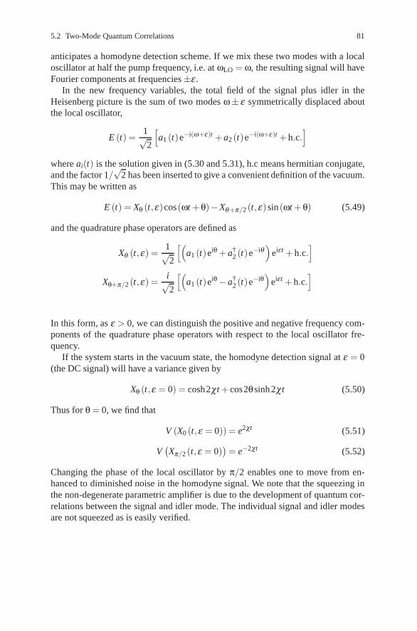
5.2 Two-Mode Quantum Correlations 81
anticipates a homodyne detection scheme. If we mix these two modes with a localoscillator at half the pump frequency, i.e. at ωLO = ω, the resulting signal will haveFourier components at frequencies±ε .
In the new frequency variables, the total field of the signal plus idler in theHeisenberg picture is the sum of two modes ω± ε symmetrically displaced aboutthe local oscillator,
E (t) =1√2
[a1 (t)e−i(ω+ε)t + a2 (t)e−i(ω+ε)t + h.c.
]
where ai(t) is the solution given in (5.30 and 5.31), h.c means hermitian conjugate,and the factor 1/
√2 has been inserted to give a convenient definition of the vacuum.
This may be written as
E (t) = Xθ (t,ε)cos(ωt + θ)−Xθ+π/2 (t,ε) sin(ωt + θ) (5.49)
and the quadrature phase operators are defined as
Xθ (t,ε) =1√2
[(a1 (t)eiθ + a†
2 (t)e−iθ)
eiεt + h.c.]
Xθ+π/2 (t,ε) =i√2
[(a1 (t)eiθ−a†
2 (t)e−iθ)
eiεt + h.c.]
In this form, as ε > 0, we can distinguish the positive and negative frequency com-ponents of the quadrature phase operators with respect to the local oscillator fre-quency.
If the system starts in the vacuum state, the homodyne detection signal at ε = 0(the DC signal) will have a variance given by
Xθ (t,ε = 0) = cosh2χt + cos2θsinh2χt (5.50)
Thus for θ = 0, we find that
V (X0 (t,ε = 0)) = e2χt (5.51)
V(Xπ/2 (t,ε = 0)
)= e−2χt (5.52)
Changing the phase of the local oscillator by π/2 enables one to move from en-hanced to diminished noise in the homodyne signal. We note that the squeezing inthe non-degenerate parametric amplifier is due to the development of quantum cor-relations between the signal and idler mode. The individual signal and idler modesare not squeezed as is easily verified.

82 5 Quantum Phenomena in Simple Systems in Nonlinear Optics
5.2.3 Quadrature Correlations and the Einstein–Podolsky–RosenParadox
The non-degenerate parametric amplifier can also be used to prepare states similar tothose discussed in the Einstein–Podolsky–Rosen (EPR) paradox [3]. In the originaltreatment two systems are prepared in a correlated state. One of two canonicallyconjugate variables is measured on one system and the correlation is such that thevalue for a physical variable in the second system may be inferred with certainty.
To see how this behaviour is manifested in the non-degenerate parametric am-plifier we first define two sets, one for each mode, of canonically conjugate vari-ables, i.e.,
Xθi = aieiθ + a†
i e−iθ (i = 1,2) . (5.53)
The variables Xθi and Xθ+π/2
i obey the commutation relation
[Xθ
i ,Xθ+π/2i
]=−2i (5.54)
and are thus directly analogous to the position and momentum operators discussedin the original EPR paper.
To measure the degree of correlation between the two modes in terms of theseoperators, we consider the quantity
V (θ ,φ)≡ 12〈(Xθ
1 −Xφ2 )2〉 . (5.55)
If V (θ ,φ) = 0 then Xθ1 is perfectly correlated with Xφ
2 . This means a measurement
of Xθ1 can be used to infer a value of Xφ
2 with certainty. To appreciate why such acorrelation should occur in the non-degenerate parametric amplifier, we can writethe interaction Hamiltonian directly in terms of the defined canonical variables,
HI =−2�χ sin(θ + φ)(
Xθ1 Xφ
2 −Xθ+π/21 Xφ+π/2
2
)
−2�χ cos(θ + φ)(
Xθ+π/21 Xφ
2 + Xθ1 Xφ+π/2
2
). (5.56)
The Heisenberg equation of motion for Xθ1 is then
Xθ1 =−4χ
[Xφ
2 cos(θ + φ)−Xφ+π/22 sin(θ + φ)
](5.57)
and we see that Xθ1 is coupled solely to Xφ
2 when θ + φ = 0.Direct calculation of V (θ ,φ) using the solutions in (5.30 and 5.31) gives
V (θ ,φ) = cosh2χt− sinh2χt cos(θ + φ) . (5.58)
When θ + φ = 0, V (θ ,φ) = e−2χt and, for long times, V (θ ,φ) becomes increas-ingly small reflecting the build up of correlation between the two variables for this
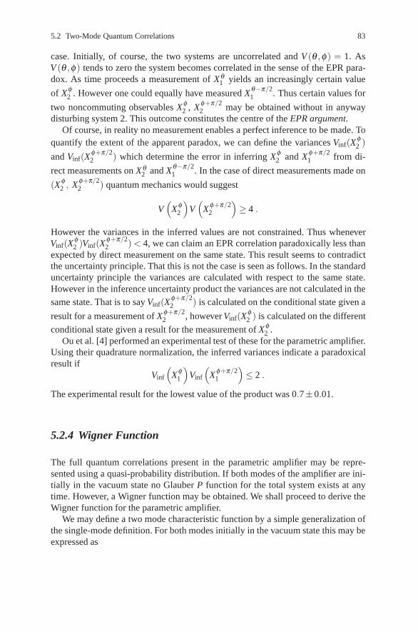
5.2 Two-Mode Quantum Correlations 83
case. Initially, of course, the two systems are uncorrelated and V (θ ,φ) = 1. AsV (θ ,φ) tends to zero the system becomes correlated in the sense of the EPR para-dox. As time proceeds a measurement of Xθ
1 yields an increasingly certain value
of Xφ2 . However one could equally have measured Xθ−π/2
1 . Thus certain values for
two noncommuting observables Xφ2 , Xφ+π/2
2 may be obtained without in anywaydisturbing system 2. This outcome constitutes the centre of the EPR argument.
Of course, in reality no measurement enables a perfect inference to be made. Toquantify the extent of the apparent paradox, we can define the variances Vinf(X
φ2 )
and Vinf(Xφ+π/22 ) which determine the error in inferring Xφ
2 and Xφ+π/21 from di-
rect measurements on Xθ2 and Xθ−π/2
1 . In the case of direct measurements made on
(Xφ2 , Xφ+π/2
2 ) quantum mechanics would suggest
V(
Xφ2
)V(
Xφ+π/22
)≥ 4 .
However the variances in the inferred values are not constrained. Thus wheneverVinf(X
φ2 )Vinf(X
φ+π/22 ) < 4, we can claim an EPR correlation paradoxically less than
expected by direct measurement on the same state. This result seems to contradictthe uncertainty principle. That this is not the case is seen as follows. In the standarduncertainty principle the variances are calculated with respect to the same state.However in the inference uncertainty product the variances are not calculated in the
same state. That is to say Vinf(Xφ+π/22 ) is calculated on the conditional state given a
result for a measurement of Xφ+π/22 , however Vinf(X
φ2 ) is calculated on the different
conditional state given a result for the measurement of Xφ2 .
Ou et al. [4] performed an experimental test of these for the parametric amplifier.Using their quadrature normalization, the inferred variances indicate a paradoxicalresult if
Vinf
(Xφ
1
)Vinf
(Xφ+π/2
1
)≤ 2 .
The experimental result for the lowest value of the product was 0.7±0.01.
5.2.4 Wigner Function
The full quantum correlations present in the parametric amplifier may be repre-sented using a quasi-probability distribution. If both modes of the amplifier are ini-tially in the vacuum state no Glauber P function for the total system exists at anytime. However, a Wigner function may be obtained. We shall proceed to derive theWigner function for the parametric amplifier.
We may define a two mode characteristic function by a simple generalization ofthe single-mode definition. For both modes initially in the vacuum state this may beexpressed as
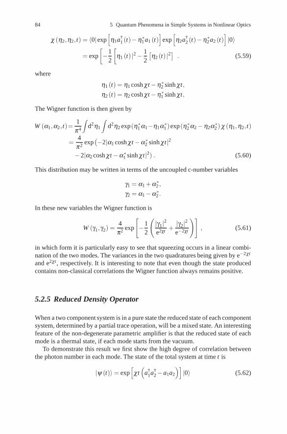
84 5 Quantum Phenomena in Simple Systems in Nonlinear Optics
χ (η2,η2,t) = 〈0|exp[η1a†
1 (t)−η∗1 a1 (t)]
exp[η2a†
2 (t)−η∗2 a2 (t)]|0〉
= exp
[−1
2
[η1 (t) |2− 1
2
[η2 (t) |2] . (5.59)
where
η1 (t) = η1 cosh χt−η∗2 sinh χt,
η2 (t) = η2 cosh χt−η∗1 sinh χt,
The Wigner function is then given by
W (α1,α2,t)=1
π4
∫d2η1
∫d2η2 exp(η∗1 α1−η1α∗1 )exp(η∗2 α2−η2α∗2 )χ (η1,η2,t)
=4
π2 exp(−2|α1 cosh χt−α∗2 sinh χt|2
−2|α2 cosh χt−α∗1 sinh χt|2) . (5.60)
This distribution may be written in terms of the uncoupled c-number variables
γ1 = α1 + α∗2 ,
γ2 = α1−α∗2 .
In these new variables the Wigner function is
W (γ1,γ2) =4π2 exp
[−1
2
(|γ1|2e2χt +
|γ2|2e−2χt
)], (5.61)
in which form it is particularly easy to see that squeezing occurs in a linear combi-nation of the two modes. The variances in the two quadratures being given by e−2χt
and e2χt , respectively. It is interesting to note that even though the state producedcontains non-classical correlations the Wigner function always remains positive.
5.2.5 Reduced Density Operator
When a two component system is in a pure state the reduced state of each componentsystem, determined by a partial trace operation, will be a mixed state. An interestingfeature of the non-degenerate parametric amplifier is that the reduced state of eachmode is a thermal state, if each mode starts from the vacuum.
To demonstrate this result we first show the high degree of correlation betweenthe photon number in each mode. The state of the total system at time t is
|ψ (t)〉= exp[χt(
a†1a†
2−a1a2
)]|0〉 (5.62)

5.2 Two-Mode Quantum Correlations 85
We now make use of the disentangling theorem [5]
eθ(
a†1a†
2−a1a2
)= eΓa†
1a†2 e−g
(a†
1a1+a†2a2+1
)e−Γa1a2 , (5.63)
whereΓ = tanh θ ,
g = ln(cosh θ ).
Thus
|ψ (t)〉= e−geΓa†1a†
2 |0〉= (cosh χt)−1∞
∑n=1
(tanh χt)n |n,n〉 , (5.64)
where |n,n〉≡ |n〉1⊗ |n〉2. As photons are created in pairs there is perfect correlationbetween the photon number in each mode. The reduced state of either mode is theneasily seen to be
ρi (t) = Tr j {|Ψ(t)〉〈Ψ(t) |}= (cosh χt)−2∞
∑n=0
(tanh χt)2n |n〉i〈n| i �= j . (5.65)
This is a thermal state with mean n = sinh2 χt, having strong analogies with theHawking effect associated with the thermal evaporation of black holes.
Suppose, however, that a photodetector with quantum efficiency μ has countedm photons in mode b. What is the state of mode a conditioned on this result? Sucha conditional state for mode a is referred to as the selected state as it is selectedfrom an ensemble of systems each with different values for the number of photonscounted in mode b. We shall now describe how the conditional state of mode a maybe calculated.
In Chap. 3 we saw that the probability to detect m photons from a field with thephoton-number distribution P(n) and detector efficiency μ is
Pμ (m) =∞
∑n=m
(nm
)(1− μ)n−m μmP1 (n) , (5.66)
where P1(n) is the photon number distribution for the field. This equation may bewritten as
Pμ (m)≈ Tr{
ρϒ†μ (m)ϒμ (m)
}(5.67)
and the operator ϒ on mode b is defined by
ϒμ (m) =∞
∑n=m
(nm
)1/2
(1− μ)(n−m)/2 μm/2|n−m〉b〈n| . (5.68)
Note that when μ → 1 this operator approaches the projection operator |0〉b〈m|.This is quite different to the projection operator |m〉b〈m| that a naive application ofthe von Neumann projection postulate would indicate for photon counting measure-ments, and reflects the fact that real photon-counting measurements are destructive,

86 5 Quantum Phenomena in Simple Systems in Nonlinear Optics
Fig. 5.2 Photon number distribution for mode a given that 5 photons are counted in mode b of aparametric amplifier. (a) μ = 0.9. (b) μ = 0.6
i.e. photons are absorbed upon detection. The conditional state of mode a is thengiven by
ρ (m) =(Pμ (m)
)−1 Trb
{ϒμ (m)ρ ϒ†
m (m)}
. (5.69)
This equation is a generalisation of the usual projection postulate. In the case of thecorrelated two mode state in (5.65), the conditional state of mode a becomes
ρ (m) =(Pμ (m)
)−1∞
∑n=m
(nm
)μm (1− μ)n−m |n〉〈n| , (5.70)
withPμ (m) = (1 + n)−1 (λ μ)m [1−λ (1− μ)](m+1) , (5.71)
where λ = tanh2 χt, n = sinh2 χt. Equation (5.70) represents a state with at leastm quanta. In Fig. 5.2 we show the photon number distribution P(m)(n) for this con-ditional state. As one would expect, when μ → 1, this approaches a number state|m〉. It should be noted, however, that the conditional state computed above refersto a situation in which the counting is done after the interaction which producesthe correlated state, is turned off. In a cavity configuration, however, it is likely thatphoton counting is proceeding simultaneously with the process of parametric ampli-fication. In that case one must proceed a little differently, however the overall resultis much the same, i.e., mode a is left with at least m quanta. The details of this morecomplicated calculation will be found in the paper by Holmes et al. [6].
5.3 Quantum Limits to Amplification
The non-degenerate parametric amplifier exemplifies many features of general lin-ear amplification. One such feature is the limit placed on the amplifier gain if theoutput is to be squeezed. To see how this limit arises, and to see how it might beovercome, we write the solutions (5.30 and 5.31) in the form

5.3 Quantum Limits to Amplification 87
Xθ1,OUT = G1/2Xθ
1, IN +(G−1)1/2 Xθ2, IN , (5.72)
where G = cosh2 χt and the quadrature phase operators are defined in (5.53). Thesubscript IN denotes operators defined at t = 0 and the subscripts 1 and 2 referto the signal and idler modes, respectively. In (5.72) the first term describes theamplification of the quadrature and the second term the noise added by the amplifier.The variances obey the equation
V(
Xθ1,OUT
)= GV
(Xθ
1, IN
)+(G−1)V
(Xθ
2, IN
). (5.73)
The maximum gain consistent with any squeezing at the output is
GMAX =1 +V
(Xθ
2, IN
)
V(
Xθ1, IN
)+V
(Xθ
2, IN
) . (5.74)
If the idler mode is in the vacuum state, V (Xθ2, IN) = 1 then
GMAX =2
1 +V(
Xθ1, IN
) , (5.75)
which gives a maximum gain of 2 for a highly squeezed state at the signal input. Forhigher values of the gain the squeezing at the signal output is lost due to contamina-tion from the amplification of vacuum fluctuation in the idler input.
Greater gains may be achieved while still retaining the squeezing in the outputsignal if the input to the idler mode, is squeezed (V (Xθ
1, IN) < 1).If we define the total noise in the signal as the sum of the noise in the two quadra-
turesN = Var
{Xθ
1
}+ Var
{Xθ+π/2
1
}(5.76)
thenNOUT = G(NIN + A) , (5.77)
where
A =(
1− 1G
)(Var
{Xθ
2, IN
}+ Var
{Xθ+π/2
2, IN
})
≤ 2
(1− 1
G
). (5.78)
This is in agreement with a general theorem for the noise added by a linear am-plifier [7]. The minimum added noise A = 2(1− 1/G) occurs when Var(Xθ
2, IN) =
Var(Xθ+π/22, IN ) = 1, that is, when the idler is in a coherent or vacuum state.

88 5 Quantum Phenomena in Simple Systems in Nonlinear Optics
5.4 Amplitude Squeezed State with PoissonPhoton Number Statistics
Finally we consider a simple nonlinear optical model which produces an amplitudesqueezed state which has Poissonian photon number statistics [8, 9]. The modeldescribes a quantised field undergoing a self-interaction via the Kerr effect. TheKerr effect is a nonlinear process involving the third-order nonlinear polarisabilityof a nonlinear medium. The field undergoes an intensity dependent phase shift, andthus we regard the medium as having a refractive index proportional to the intensityof the field.
Quantum mechanically the Kerr effect may be described by the effective Hamil-tonian
H = �χ2
(a†)2
a2 , (5.79)
where χ is proportional to the third-order nonlinear susceptibility. The Heisenbergequation of motion for the annihilation operator is
dadt
=−iχa†a a . (5.80)
As a†a, the photon number operator, is a constant of motion the photon numberstatistics is time invariant. The solution is then
a(t) = e−iχta†aa(0) . (5.81)
Assume the initial state is a coherent state with real amplitude α . The mean ampli-tude at a later time is then
〈a(θ )〉= α exp[−α2 (1− cosθ )− iα2 sinθ
], (5.82)
where we have defined θ = χt. Typically θ � 1 and then
〈a(θ )〉 ≈ αe−iα2θ−α2θ 2/2 . (5.83)
This result displays two effects. Firstly, there is a rotation of the mean amplitudeby α2θ ; the expected nonlinear phase shift. Secondly, there is a decay of the am-plitude which goes quadratically with time. This decay is due to the fact that theKerr effect transforms intensity fluctuations in the initial coherent state into phasefluctuations (Fig. 5.3). In effect, the initial coherent state error circle undergoes arotational shearing while the area remains constant.
Inspection of Fig. 5.3 suggests that, at least for short times, this system is likelyto produce a squeezed state with reduced amplitude fluctuations. This is indeed thecase. For short times (θ � 1) and large intensities (α2� 1) one finds the minimumvariance of the in-phase quadrature approaches the value
V (X1)min = 0.4 . (5.84)

5.4 Amplitude Squeezed State with Poisson Photon Number Statistics 89
Fig. 5.3 Contour of theQ-function (at a height of0.3) for the state of a singlemode, prepared in a coherentstate with α = 2.0, evolvedwith a Kerr nonlinearity forθ = 0.25. The equivalent con-tour for the initial coherentstate is shown as dashed
-3 -2 -1 0 1 2 3-3
-2
-1
0
1
2
3
X1
X2
This occurs at the value
θmin ≈±0.55α2 . (5.85)
This short time behaviour is evident in Fig. 5.4a. Thus even though the photon statis-tics is at all times Poissonian, for short times the field is amplitude squeezed.
We now consider mixing the output of the nonlinear process with a coherent fieldon a beam splitter of low reflectivity. The output field is now given by
a0 =√
T e−iθa†aa +√
Rβ , (5.86)
where β is the coherent amplitude of the mixing field, and T and R are, respec-tively, the transmitivity and reflectivity of the beam splitter. We assume T → 1 with√
Rβ → ξ , that is the mixing field is very strong. In this limit we have
a0 = e−iθa†aa + ξ . (5.87)
We now can choose ξ so as to minimise the photon number noise at the output.This requires ξ to be −π/2 out-of-phase with the coherent excitation of the input.As θ increases, the ratio of the number variance to number mean decreases to aminimum at θ = 1/2〈n0〉−2/3 (for optimal ξ ), and then increases. The minimumphoton number variance is [10]
V (n0) = 〈n0〉1/3 , (5.88)
where 〈n0〉= 〈n〉+ |ξ |2. This is smaller than the similar result for a squeezed state,which has a minimum value of 〈n〉2/3.

90 5 Quantum Phenomena in Simple Systems in Nonlinear Optics
Fig. 5.4 A plot of the variancein the in-phase quadrature forthe Kerr interaction, versusthe dimensionless interactiontime θ , with an initial coher-ent state of amplitude α = 4.0.(a) Short time behaviour. (b)Long time behaviour
Were the rotational shearing to continue (as one might expect from a classicalmodel) the variance in the in-phase and out-of-phase quadratures would saturate atthe value 2α2 + 1. This would be the variance for a number state with the photonnumber equal to α2. That this does not happen is evident in Fig. 5.4b. Indeed, from(5.82) it is clear that for θ = 2π the mean amplitude returns to the initial value. Asimilar result holds for the variances (Exercise 5.6). This is an example of a quantumrecurrence and arises from the discrete nature of the photon number distribution fora quantised field. The details are left for Exercise 5.6. In fact at θ = π the systemevolves to a coherent superposition of coherent states:
|ψ (θ = π)〉|= 1√2
(eiπ/4|iα〉+ e−iπ/4|− iα〉
). (5.89)
This phenomenon would be very difficult to observe experimentally as typical val-ues of χ would require absurdly large interaction times, which in practice meansextremely large interaction lengths. In Chap. 15 we will show that dissipation alsomakes the observation of such a coherent superposition state unlikely in a Kerrmedium.

References 91
Exercises
5.1 Derive the Wigner and P functions for the reduced density operator of thesignal mode for the non-degenerate parametric amplifier.
5.2 Show that, n1− n2, the difference in the number of photons in the signal andidler mode is a constant for the parametric amplifier.
5.3 The Hamiltonian for the frequency up-converter is
H = �ω1a†1a1 +�ω2a†
2a2 +�κ(
eiωt a†1a2 + e−iωta1a†
2
),
where ω = ω2−ω1. Show that n1 + n2, the sum of the number of photons inthe signal and idler modes, is a constant.
5.4 Show that the process of parametric frquency upconversion is noiseless, thatis a coherent state remains coherent.
5.5 Take the initial state for the frequency upconverter to be |N,N〉. Express thedensity operator at time t as the tensor product of number states. Hint: Use thedisentangling theorem, see (5.63). What is the reduced density operator for asingle mode?
5.6(a) If the initial state for the Kerr-effect model is a coherent state with realmean amplitude, calculate the variances for the in-phase and out-of-phasequadratures. Show that at χt = π the field exhibits amplitude squeezing forsmall values of the amplitude.
(b) Show that at χt = π the state may be written in the form
1√2
(eiπ/4|− iα〉+ e−iπ/4|iα
).
References
1. B.R. Mollow, R.J. Glauber: Phys. Rev. 160, 1097 (1967); ibid. 162, 1256 (1967)2. B.L. Schumaker, C.M. Caves: Phys. Rev. A 31, 3093 (1985)3. M.D. Reid, P.D. Drummond: Phys. Rev. Lett. A 41, 3930 (1990)4. Z.Y. Ou, L. Mandel: Phys. Rev. Lett. 61, 50 (1988)5. M.J. Collett: Phys. Rev. A 38, 2233 (1988)6. C.A. Holmes, G.J. Milburn, D.F. Walls: Phys. Rev. A 39, 2493 (1989)7. C.M. Caves: Phys. Rev. D 26, 1817 (1982)8. G.J. Milburn: Phys. Rev. A 33, 674 (1985)9. B. Yurke, D. Stoler: Phys. Rev. Lett. 57, 13 (1985)
10. M. Kitagawa, Y. Yamamoto: Phys. Rev. A 34, 345 (1986)

Chapter 6Stochastic Methods
Abstract In all physical processes there is an associated loss mechanism. In thischapter we shall consider how losses may be included in the quantum mechanicalequations of motion. There are several ways in which a quantum theory of dampingmay be developed. We shall adopt the following approach: We consider the systemof interest coupled to a heat bath or reservoir. We first derive an operator masterequation for the density operator of the system in the Schrodinger or interactionpicture. Equations of motion for the expectation values of system operators maydirectly be derived from the operator master equation. Using the quasi-probabilityrepresentations for the density operator discussed in Chap. 4, the operator masterequation may be converted to a c-number Fokker–Planck equation. For linear prob-lems a time-dependent solution to the Fokker–Planck equation may be found. In cer-tain nonlinear problems with an appropriate choice of representation the steady-statesolution for the quasi-probability distribution may be found from which momentsmay be calculated.
Using methods familiar in stochastic processes the Fokker–Planck equationmay be converted into an equivalent set of stochastic differential equations. Thesestochastic differential equations of which the Langevin equations are one exampleare convenient when linearization is necessary. We begin then with a derivation ofthe master equation. We follow the method of Haake [1].
6.1 Master Equation
We consider a system described by the Hamiltonian HS coupled to a reservoir de-scribed by the Hamiltonian HR. The reservoir may be considered to be a large num-ber of harmonic oscillators as, for example, the modes of the free electromagneticfield or phonon modes in a solid. In some cases the reservoir may be more appro-priately modelled as a set of atomic energy levels. The derivation of the masterequation is not dependent on the specific reservoir model. There is a weak inter-action between the system and the reservoir given by the Hamiltonian V . Thus thetotal Hamiltonian is
93

94 6 Stochastic Methods
H = HS +HR +V (6.1)
Let w(t) be the total density operator of the system plus reservoir in the interactionpicture. The equation of motion in the interaction picture is
dw(t)dt
=− ih[V (t),w(t)] (6.2)
The reduced density operator for the system is defined by
ρ(t) = TrR{w(t)} (6.3)
where TrR indicates a trace over reservoir variables. We assume that initially thesystem and reservoir are uncorrelated so that
w(0) = ρ(0)⊗ρR (6.4)
where ρR is the density operator for the reservoir.Integrating (6.2) we obtain
w(t) = w(0)− ih
t∫0
dt1[V (t1),w(t1)] . (6.5)
Iterating this solution we find
w(t) = w(0)+∞
∑n=1
(− i
h
)n t∫0
dt1
t1∫0
dt2 · · ·
×tn−1∫0
dtn[V (t1), [V (t2), . . . [V (tn),w(0)]]] . (6.6)
Performing the trace over reservoir variables
ρ(t) = ρ(0)+∞
∑n=1
(− i
h
)n t∫0
dt1
t1∫0
dt2 · · ·tn−1∫0
dtn
×TrR{[V (t1), [V (t2), . . . [V (tn), ρR⊗ρ(0)]]]}≡ (1 +U1(t)+U2(t)+ · · ·)ρ(0) (6.7)
≡U(t)ρ(0)
where
Un(t) =(− i
h
)n
TrR
t∫0
dt1
t1∫0
dt2 · · ·
×tn−1∫0
dtn[V (t1), [V (t2), . . . [V (tn),ρR⊗ (·)]] . . .] . (6.8)
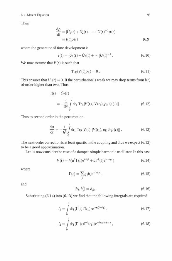
6.1 Master Equation 95
Thus
dρdt
= [U1(t)+U2(t)+ · · · ]U(t)−1ρ(t)
≡ l(t)ρ(t) (6.9)
where the generator of time development is
l(t) = [U1(t)+U2(t)+ · · · ]U(t)−1 . (6.10)
We now assume that V (t) is such that
TrR(V (t)ρR) = 0 . (6.11)
This ensures that U1(t) = 0. If the perturbation is weak we may drop terms from l(t)of order higher than two. Thus
l(t) = U2(t)
=− 1
h2
t∫0
dt1 TrR[V (t), [V (t1),ρR⊗ (·)]] . (6.12)
Thus to second order in the perturbation
dρdt
=− 1
h2
t∫0
dt1 TrR[V (t), [V (t1),ρR⊗ρ(t)]] . (6.13)
The next-order correction is at least quartic in the coupling and thus we expect (6.13)to be a good approximation.
Let us now consider the case of a damped simple harmonic oscillator. In this case
V (t) = h(a†Γ(t)eiω0t + aΓ†(t)e−iω0t) (6.14)
whereΓ(t) = ∑
j
g jb je−iω jt , (6.15)
and[b j,b
†k] = δ jk . (6.16)
Substituting (6.14) into (6.13) we find that the following integrals are required
I1 =t∫
0
dt1〈Γ(t)Γ(t1)〉eiω0(t+t1) , (6.17)
I2 =t∫
0
dt1〈Γ†(t)Γ†(t1)〉e−iω0(t+t1) , (6.18)

96 6 Stochastic Methods
I3 =t∫
0
dt1〈Γ(t)Γ†(t1)〉eiω0(t−t1) , (6.19)
I4 =t∫
0
dt1〈Γ†(t)Γ(t1)〉e−iω0(t−t1) (6.20)
which we now evaluate.Using the definition of Γ(t) we have
I1 =t∫
0
dt1 ∑i, j
gig j〈bib j〉Re−i(ωit+ω jt1)eiω0(t+t1) . (6.21)
Converting the sum over modes to a frequency-space integral
I1 =t∫
0
dt1
∞∫0
dω1
2πρ(ω1)
∞∫0
dω2
2πρ(ω2)g(ω1)g(ω2)〈b(ω1)b(ω2)〉R
× e−i(ω1t+ω2t1)+iω0(t+t1) (6.22)
where ρ(ω) is the density of states function.For a thermal bath the phase dependent correlation function 〈b(ω1)b(ω2)〉R = 0.
However, certain specially prepared reservoirs such as squeezed reservoirs may havephase-dependent correlations.
In order to include these we now assume that
〈b(ω1)b(ω2)〉= 2πM(ω1)δ (2ω0−ω1−ω2) (6.23)
which corresponds to a multimode squeezed vacuum state with the carrier frequencyequal to the cavity resonance frequency. Thus
I1 =t∫
0
dt1
∞∫0
dω2π
ρ(ω)ρ(2ω0−ω)g(ω)g(2ω0−ω)M(ω)ei(ω0−ω)(t−t1) . (6.24)
Note that the time integral depends only on t− t1. This suggests the change of vari-able τ = t− t1 and thus
I1 =t∫
0
dτ∞∫
0
dω2π
ρ(ω)ρ(2ω0−ω)g(ω)g(2ω0−ω)M(ω)ei(ω0−ω)τ . (6.25)
We now make the first Markov approximation by assuming ρ(ω), g(ω) and M(ω)are slowly varying functions around ω = ω0, where ω0 is very large. Thus it isconvenient to make the change of variable ε = ω−ω0 and write
I1 ≈t∫
0
dτ∞∫−∞
dε2π
ρ2(ε + ω0)g2(ε + ω0)M(ε + ω0)e−iετ , (6.26)
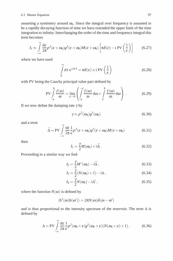
6.1 Master Equation 97
assuming a symmetry around ω0. Since the integral over frequency is assumed tobe a rapidly decaying function of time we have extended the upper limit of the timeintegration to infinity. Interchanging the order of the time and frequency integral thisterm becomes
I1 ≈∞∫−∞
dε2π
ρ2(ε + ω0)g2(ε + ω0)M(ε + ω0)[
πδ (ε)− i PV
(1ε
)](6.27)
where we have used∞∫
0
dτ e±iετ = πδ (ε)± i PV
(1ε
)(6.28)
with PV being the Cauchy principal value part defined by
PV
b∫−a
f (ω)ω
= limε→0
⎛⎝−ε∫−a
f (ω)ω
dω +b∫
ε
f (ω)ω
dω
⎞⎠ . (6.29)
If we now define the damping rate γ by
γ ≡ ρ2(ω0)g2(ω0) (6.30)
and a term
Δ = PV
∞∫−∞
dε2π
1ε
ρ2(ε + ω0)g2(ε + ω0)M(ε + ω0) (6.31)
thenI1 =
γ2
M(ω0)+ iΔ . (6.32)
Proceeding in a similar way we find
I2 =γ2
M∗(ω0)− iΔ , (6.33)
I3 =γ2(N(ω0)+ 1)− iΔ , (6.34)
I4 =γ2
N(ω0)− iΔ′ , (6.35)
where the function N(ω) is defined by
〈b†(ω)b(ω ′)〉= 2πN(ω)δ (ω −ω ′)
and is thus proportional to the intensity spectrum of the reservoir. The term Δ isdefined by
Δ = PV
∞∫−∞
dε2π
1ε
ρ2(ω0 + ε)g2(ω0 + ε)(N(ω0 + ε)+ 1) . (6.36)

98 6 Stochastic Methods
This term represents a small shift in the frequency of the oscillator. In the casewhere the system is a two-level atom, this term contributes to the Lamb shift whichwe discuss in Chap. 10. In what follows we ignore the effects of Δ and Δ.
Substituting the above results into (6.13) we find that the evolution of the sys-tem’s density operator in the interaction picture is described by the master equation
dρdt
=γ2(N + 1)(2aρa†−a†aρ−ρa†a)+
γ2
N(2a†ρa−aa†ρ−ρaa†)
+γ2
M(2a†ρa†−a†a†ρ−ρa†a†)+γ2
M∗(2aρa−aaρ−ρaa) . (6.37)
(For convenience, we have suppressed the functional dependence of N(ω0) andM(ω0)).
If the bath is in thermal equilibrium at temperature T, M = 0 and
N(ω0) = (ehω0/kT −1)−1 (6.38)
which is just the mean number of bath quanta at frequency ω0. In this case the masterequation considerably simplifies. If the bath temperature is zero, N = 0, and themaster equation simplifies further. In general the positivity of the density operatorrequires, |M|2 ≤ N(N + 1).
Equations of motion for the expectation values of system operators may be di-rectly derived from the master equation, (6.37). For example, the mean amplitudeof the simple harmonic oscillator is given by
d〈a〉dt
= Tr
{a
dρdt
}=− γ
2〈a〉 (6.39)
which has the solution〈a(t)〉= 〈a(0)〉e−γt/2 . (6.40)
(Note in the Schrodinger picture the mean amplitude evolves as 〈a(t)〉= 〈a(0)〉e−iωt
e−γt/2). Thus the mean amplitude decays at a rate γ/2. The mean number of quanta〈n〉= 〈a†a〉 obeys the equation
d〈a†a〉dt
=−γ〈a†a〉+ γN . (6.41)
The solution to this equation is
〈n(t)〉= 〈n(0)〉e−γt + N(1− e−γt) . (6.42)
In the steady state 〈n(t)〉 → N and the mean number of quanta in the oscillator isequal to the mean number of quanta in the reservoir at that temperature. The role ofthe terms multiplied by M can be seen by evaluating the equation of motion for 〈a2〉,
ddt〈a2〉=−γ〈a2〉+ γM . (6.43)

6.2 Equivalent c-Number Equations 99
Thus these terms lead to a driving force on the second-order phase dependentmoments.
The master equation (6.37) applies to a free damped harmonic oscillator in theinteraction picture. If the harmonic oscillator is perturbed by an additional interac-tion HI, the master equation in the interaction picture becomes
dρdt
=− l
h[HI ,ρ ]+
γ2(N + 1)(2aρa†−a†aρ−ρa†a)
+γ2
N(2a†ρa−aa†ρ−ρaa†)
+γ2
M(2a†ρa†− (a†)2ρ−ρ(a†)2)+γ2
M∗(2aρa−a2ρ−ρa2) .
(6.44)
In general, the equations of motion for the mean amplitude, mean quantum numberetc. are not as easily obtained from (6.44), as they were for the free damped har-monic oscillator. To proceed in such situations, it is desirable to convert the masterequation to an equivalent c-number partial differential equation. We now discussvarious ways this may be done.
6.2 Equivalent c-Number Equations
6.2.1 Photon Number Representation
The operator master equation may be converted into an equation for the matrixelements of ρ in the number state basis:
∂ρmn
∂ t= γN[(nm)1/2ρm−1, n−1− 1
2(m+ n + 2)ρmn].
+ γ(N + 1){[(m+ 1)(n + 1)]1/2ρm+1, n+1− 12(m+ n)ρmn}
− γ2
M{
2[m(n + 1)]1/2ρm−1, n+1−√
(n + 1)(n + 2)ρm,n+2
−√
m(m−1)ρm−2, n
}− γ
2M∗
{2[n(m+ 1)]1/2ρm+1,n−1
−√
(m+ 1)(m+ 2)ρm+2, n−√
n(n−1)ρm,n−2
}(6.45)
where ρm, n ≡ 〈m|ρ |n〉. This gives an infinite hierarchy of coupled equations for theoff-diagonal matrix elements. When M = 0 the diagonal elements ρm, m are coupledonly amongst themselves and not coupled to the off-diagonal elements. In this casethe diagonal elements satisfy
dP(n)dt
= t+(n−1)P(n−1)+ t−(n + 1)P(n + 1)− [t+(n)+ t−(n)]P(n) (6.46)

100 6 Stochastic Methods
where we have set P(n) = 〈n|ρ |n〉 and defined the transition probabilities
t+(n)≡ γN(n + 1) , (6.47)
t−(n)≡ γ(N + 1)n . (6.48)
In the steady state the detailed balance condition holds:
t−(n)P(n) = t+(n−1)P(n−1) (6.49)
and the steady state solution is found by iteration
Pss(n) = P(0)n
∏k=1
t+(k−1)t−(k)
. (6.50)
Thus the steady state solution for the ordinary damped harmonic oscillator(M = 0) is
Pss(n) =1
1 + N
(N
1 + N
)n
. (6.51)
An optical cavity damped into a reservoir with phase-independent correlation func-tions has a power law photon number distribution of thermal light.
In the more general case M �= 0, or when there are additional terms in the masterequation such as linear driving with the Hamiltonian H0 = h[ε(t)a† + ε∗(t)a], thecoupling of diagonal and off-diagonal matrix elements makes the photon numberrepresentation less convenient for determining ρ(t).
6.2.2 P Representation
An operator master equation may be transformed to a c-number equation using theGlauber–Sudarshan representation for ρ . It is necessary to first establish the rulesfor converting operators to an equivalent c-number form. We know the relations
a|α〉= α|α〉 , (6.52)
〈α|a† = α∗〈α| . (6.53)
To derive other relations it is convenient to use the Bargmann state ‖ α〉 defined by
‖ α〉= e1/2|α |2 |α〉 (6.54)
so that
a† ‖ α〉= ∑n
αn√
n!
√n + 1|n + 1〉
=∂
∂α‖ α〉 . (6.55)

6.2 Equivalent c-Number Equations 101
Similarly
〈α ‖ a =∂
∂α∗〈α ‖ . (6.56)
Hence, given the P representation
ρ =∫
d2α ‖ α〉〈α ‖ e−|α |2
P(α) (6.57)
we find
a†ρ =∫
d2α∂
∂α(‖ α〉〈α ‖)e−αα∗ P(α) (6.58)
and integrating by parts
a†ρ =∫
d2α ‖ α〉〈α ‖ e−|α |2(
α∗ − ∂∂α
)P(α) . (6.59)
We can thus make an operator correspondence between a† and α∗ − ∂/∂α . A sim-ilar formula holds for a. Summarizing we have the following operator correspon-dences:
aρ ↔ αP(α),
a†ρ ↔(
α∗ − ∂∂α
)P(α),
ρa↔(
α− ∂∂α∗
)P(α),
ρa†↔ α∗P(α) . (6.60)
Consider the correspondences for operator products
a†aρ →(
α∗ − ∂∂α
)αP , (6.61a)
ρa†a→(
α− ∂∂α∗
)α∗P . (6.61b)
Notice that the order of the operators in (6.61b) reverses, since acting on ρ , theyoperate from the right, whereas on P, they operate from the left.
Note that α and α∗ are not independent variables. In terms of real variables wemay write
α = x + iy,
α∗ = x− iy,
∂∂α
=12
(∂∂x− i
∂∂y
),
∂∂α∗
=12
(∂∂x
+ i∂∂y
). (6.62)

102 6 Stochastic Methods
To obtain a c-number equation we substitute the P representation for ρ into themaster equation and use the operator correspondences. This leads to the equation
∂P(α)∂ t
=[
12
γ(
∂∂α
α +∂
∂α∗α∗
)+
γ2
(M∗
∂ 2
∂α∗2+ M
∂ 2
∂α2
)+ γN
∂ 2
∂α∂α∗
]P(α) .
(6.63)
When M > N this equation has “non positive-definite” diffusion, hence the P repre-sentation is unable to describe the system in terms of a classical stochastic process.Alternative representations will be discussed later in this chapter. When M ≤ N(6.63) has the form of a Fokker–Planck equation. We shall discuss some usefulproperties of Fokker–Planck equations below.
6.2.3 Properties of Fokker–Planck Equations
A general Fokker–Planck equation in n variables may be written in the form
∂∂ t
P(x) =[− ∂
∂x jA j(x)+
12
∂∂xi
∂∂x j
Di j(x)]
P(x) . (6.64)
The first derivative term determines the mean or deterministic motion and is calledthe drift term, while the second derivative term, provided its coefficient is positivedefinite, will cause a broadening or diffusion of P(x, t) and is called the diffusionterm. A = (A j) is the drift vector and D = (Di j) is the diffusion matrix. The differentrole of the two terms may be seen in the equations of motion for 〈xk〉 and 〈xkxl〉.
d〈xk〉dt
= 〈Ak〉 , (6.65)
d〈xkxl〉dt
= 〈xkAl〉+ 〈xlAk〉+ 12〈Dkl + Dlk〉 . (6.66)
We see that Ak determines the motion of the mean amplitude whereas Dlk enters intothe equation for correlations.
Thus, for the damped harmonic oscillator described by (6.63)
d〈α〉Pdt
=− γ2〈α〉P , (6.67)
d〈α∗α〉Pdt
=−γ〈α∗α〉P + γN , (6.68)
which are equivalent to (6.39 and 6.41) derived directly from the master equa-tion (6.37). Note that the expectation values 〈〉P are defined by integrals overP(α, t).

6.2 Equivalent c-Number Equations 103
6.2.4 Steady State Solutions – Potential Conditions
For many problems in nonlinear optics it is sufficient to know the steady state solu-tion. That is the solution after all transients have died out. We shall therefore seek asteady state solution to (6.64).
In the steady state we set the time derivatives to zero which gives
∂∂xi
[−Ai(x)P(x)+
12
∂∂x j
Di j(x)P(x)]
= 0 . (6.69)
As a first attempt consider
Ai(x)P(x) =12
∂∂x j
[Di j(x)P(x)] (6.70)
which implies
Di j∂ lnP∂x j
= 2Ai(x)− ∂Di j
∂x j(x) . (6.71)
Denoting P(x) = exp[−φ(x)] we wish to solve
−∂φ(x)∂xi
= 2(D−1)i j
[A j(x)− 1
2
∂D jk
∂xk
]≡ Fi(x) . (6.72)
If we consider Fj(x) as a generalized force, φ(x) corresponds to a potential. Thesystem of equations (6.72) can be solved by integration if the so called potentialconditions are satisfied
−∂ 2φ∂xi∂x j
=∂Fj
∂xi=
∂Fi
∂x j=−∂ 2φ∂x j∂xi
. (6.73)
These conditions say that the function φ is well behaved and that the multivariableintegral is independent of the path of integration. The potential conditions are alwayssatisfied in the one dimensional case.
Provided the potential conditions are satisfied a steady state solution of the form
P(x) = N exp[−φ(x)] (6.74)
exists where
φ(x) =x∫
0
2[D(x)−1]i j
[−A j(x)+
12
∂D jk
∂xk
]dxi .
The turning points of the potential φ correspond to the values x such that for eachj = 1, . . . , n (
A j(x)− 12
∂D jk(x)∂xk
)= 0 . (6.75)

104 6 Stochastic Methods
In systems where the diffusion matrix is diagonal and constant (Di j = Wδi j) (6.72)become
−∂φ(x)∂xi
=2Ai(x)
W. (6.76)
Hence the turning points of the potential φ correspond exactly to the determinis-tic steady state solutions, that is the steady state solutions to the first-order momentequations.
6.2.5 Time Dependent Solution
In the case where the drift term is linear in the variable (x) and the diffusion coef-ficient is a constant, a solution to the Fokker–Planck equation may be found usingthe method of Wang and Uhlenbeck [2]. We consider the Fokker–Planck equation
∂P∂ t
=−∑ai∂
∂xi(xiP)+
12
di j∂ 2P
∂xi∂x j. (6.77)
The Greens function solution to this equation given by the initial condition
P(xi,0) = δ (xi− x0i )
is
P(xi,x0i ,t) =
1
πn/2[det σi j(t)]1/2exp
(−∑
i j
σi j(t)−1{[xi− x0i exp(ait)]
×[x j− x0j exp(a jt)]}
)(6.78)
where
σi j(t) =−2di j
ai + a j{1− exp[(ai + a j)t]} .
The solution for a damped harmonic oscillator initially in a coherent state withP(α, 0) = δ 2(α−α0) is
P(α,t) =1
πN(1− e−γt)exp
(−|α−α0e−γt/2|2
N(1− e−γt)
). (6.79)
This represents an initial coherent state undergoing relaxation with a heat bath. Itscoherent amplitude decays away and fluctuations from the heat bath cause its Pfunction to assume a Gaussian form characteristic of thermal noise. The width ofthe distribution grows with time until the oscillator reaches equilibrium with theheat bath.
From the above solution we may construct solutions for all initial conditionswhich have a non-singular P representation. It is not, however, possible to construct
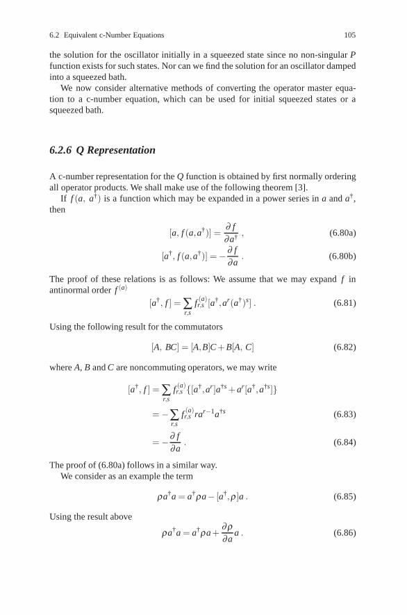
6.2 Equivalent c-Number Equations 105
the solution for the oscillator initially in a squeezed state since no non-singular Pfunction exists for such states. Nor can we find the solution for an oscillator dampedinto a squeezed bath.
We now consider alternative methods of converting the operator master equa-tion to a c-number equation, which can be used for initial squeezed states or asqueezed bath.
6.2.6 Q Representation
A c-number representation for the Q function is obtained by first normally orderingall operator products. We shall make use of the following theorem [3].
If f (a, a†) is a function which may be expanded in a power series in a and a†,then
[a, f (a,a†)] =∂ f∂a† , (6.80a)
[a†, f (a,a†)] =−∂ f∂a
. (6.80b)
The proof of these relations is as follows: We assume that we may expand f inantinormal order f (a)
[a†, f ] = ∑r,s
f (a)r,s [a†,ar(a†)s] . (6.81)
Using the following result for the commutators
[A, BC] = [A,B]C + B[A, C] (6.82)
where A, B and C are noncommuting operators, we may write
[a†, f ] = ∑r,s
f (a)r,s {[a†,ar]a†s + ar[a†,a†s]}
=−∑r,s
f (a)r,s rar−1a†s (6.83)
=−∂ f∂a
. (6.84)
The proof of (6.80a) follows in a similar way.We consider as an example the term
ρa†a = a†ρa− [a†,ρ ]a . (6.85)
Using the result above
ρa†a = a†ρa +∂ρ∂a
a . (6.86)

106 6 Stochastic Methods
Taking matrix elements in coherent states yields
〈α|ρa†a|α〉= α⟨
α∣∣∣∣a†ρ +
∂ρ∂a
∣∣∣∣α⟩
=(|α|2 + α
∂∂α
)Q(α) . (6.87)
Following this procedure we may convert the master equation for the damped har-monic oscillator into a c-number equation for the Q function
∂Q∂ t
=γ2
(∂
∂αα+
∂∂α∗
α∗)
Q+γ2
[M∗
∂ 2
∂α∗2 + M∂ 2
∂α2 + 2(N + 1)∂ 2
∂α∂α∗
]Q .
(6.88)
This differs from the corresponding equation of motion for the P function onlythrough the phase independent diffusion coefficient which is N + 1 rather than N.This is sufficient to give a positive definite diffusion matrix when the bath is in anideal squeezed state.
To illustrate the use of the Q function consider a damped oscillator which isinitially in the squeezed state |α0, r〉. Using the Wang and Uhlenbeck solution foran initial δ -function and convoluting this with the Gaussian Q function for an initialsqueezed state we arrive at the result
Q(α, t) =1
2π√
det σ(t)exp[−1
2u(t)Tσ−1(t)u(t)] (6.89)
where
u(t) =(
α−α0e−γt/2
α∗ −α∗0 e−γt/2
)
σ(t) =( −sinh 2r cosh 2r + 1
cosh 2r + 1 −sinh 2r
)e−γt
2+(
M N + 1N + 1 M∗
)(1− e−γt).
The variances for the quadrature phase operators Xi for the oscillator are then easilyfound to be
V (X1) =14[(e−2r−1)e−γt + 2(N + Re{M})(1− e−γt)+ 1] , (6.90a)
V (X2) =14[(e2r + 1)e−γt + 2(N + Re{M})(1− e−γt)+ 1] . (6.90b)
In Fig. 6.1 we depict the evolution of an initial squeezed state coupled to a zerotemperature reservoir (N = M = 0). The amplitude of the squeezed state dampsto zero and the variances in X1 and X2 become equal at the value one correspondingto the vacuum.

6.2 Equivalent c-Number Equations 107
Fig. 6.1 Evolution of theerror contour of an initialsqueezed state of a simpleharmonic oscillator dampedinto a zero temperatureheat bath
6.2.7 Wigner Function
Alternatively one may convert the operator master equation into a c-number equa-tion via the Wigner function. This is best accomplished by deriving an equation forthe characteristic function
χ(β ) = Tr{Dρ} (6.91)
whereD = eβ a†−β ∗a .
An equation of motion for χ(β ) may be derived as follows
∂ χ(β )∂ t
= Tr
{D
∂ρ∂ t
}. (6.92)
To illustrate the technique we shall derive the equation of motion for the Wignerfunction of a damped harmonic oscillator.
We require some operator rules to convert to differential operators. Writing D innormal order
D = e−β β ∗/2eβ a†e−β ∗a , (6.93)
∂∂β
D =−β ∗
2D+ a†D , (6.94)
or
a†D =(
∂∂β
+β ∗
2
)D . (6.95)
Similarly we may show
Da =(−β
2− ∂
∂β ∗
)D . (6.96)

108 6 Stochastic Methods
Writing D in antinormal order
D = eβ β ∗/2e−β ∗aeβ a†. (6.97)
Thus∂
∂βD =
β ∗
2D+ Da† (6.98)
or
Da† =(
∂∂β− β ∗
2
)D (6.99)
and similarly
aD =(
β2− ∂
∂β ∗
)D . (6.100)
Then using these rules the master equation (6.37) yields the following equation forthe characteristic function
∂ χ(β )∂ t
=γ2
(−|β |2−β ∗
∂∂β ∗−β
∂∂β
)χ(β )− γN|β |2χ(β )
− γM2
(β ∗)2χ(β )− γM∗
2β 2χ(β ) . (6.101)
The equation for the Wigner function is obtained by taking the Fourier transform ofthis equation since
W (α) =∫
eβ ∗α−β α∗χ(β )d2β . (6.102)
Thus∫
eβ ∗α−α∗β β ∗β χ(β )d2β =−∫ ∂
∂α∂
∂α∗(eβ ∗α−α∗β )χ(β )d2β
=−∂ 2W (α)∂α ∂α∗
, (6.103)
and∫
eβ ∗α−α∗β β ∗∂
∂β ∗χ(β )d2β =
∂∂α
∫(eβ ∗α−α∗β )
∂∂β ∗
χ(β )d2β
=− ∂∂α
∫χ(β )
∂∂β ∗
(eβ ∗α−α∗β )d2β (6.104)
=− ∂∂α
[αW (α)] . (6.105)
Using these results we may write the equation for the Wigner function as
∂W (α)∂ t
=γ2
(∂
∂αα +
∂∂α∗
α∗)
W
+γ2
[M∗
∂ 2
∂α∗2+ M
∂ 2
∂α2 + 2
(N +
12
)∂ 2
∂α ∂α∗
]W . (6.106)
6.2 Equivalent c-Number Equations 109
A comparison of the three equations (6.63, 6.88 and 6.106) for the P, Q and Wignerfunctions show that they differ only in the coefficient of the diffusion term beingγN, γ(N + 1) and γ(N + 1/2), respectively. However, the additional +γ and +γ/2in the equations for the Q and Wigner function are sufficient to ensure that theseequations have positive definite diffusion.
6.2.8 Generalized P Representation
In our study of nonlinear problems we shall find systems which either do not giveFokker–Planck equations in the Q and Wigner representations or no steady statesolution may readily be found. For some systems a steady state solution in terms ofa Glauber–Sudarshan P representation does not exist. For such systems the complexP representation is sometimes useful in deriving a steady state solution to Fokker–Planck equations. The positive P representation is useful when it is desirable to havea Fokker–Planck equation with a positive definite diffusion term, as is necessary inorder to deduce the corresponding stochastic differential equations.
Master equations may be converted to a c-number representation using the com-plex P representation by an analogous set of operator rules used for the diagonal Prepresentation.
The nondiagonal coherent state projection operator is defined as
Λ(α) =|α〉〈β ∗|〈β ∗|α〉 (6.107)
where (α) denotes (α, β ). The following identities hold
aΛ(α) = αΛ(α), a†Λ(α) =(
β +∂
∂α
)Λ(α),
Λ(α)a† = Λ(α)β , Λ(α)a =(
∂∂β
+ α)
Λ(α) . (6.108)
By substituting the above identities into (4.65) defining the generalized P repre-sentation, and using partial integration (providing the boundary terms vanish) theseidentities can be used to generate operations on the P function depending on therepresentation.
a) Complex P representation
aρ↔ αP(α), a†ρ ↔(
β − ∂∂α
)P(α),
ρa†↔ β P(α), ρa↔(
α− ∂∂β
)P(α) . (6.109)
This procedure yields a very similar equation to that for the Glauber–Sudarshan Pfunction. We assume that, by appropriate reordering of the differential operators,

110 6 Stochastic Methods
we can reduce an operator master equation to the form [where (α, β ) = (α) =(α(1), α(2))]
∂ρ∂ t
=∫c
∫
c′Λ(α)
∂P(α)∂ t
dα dβ
=∫c
∫
c′dα(1) dα(2) P(α)
[Aμ(α)
∂∂αμ +
12
Dμν(α)∂
∂αμ∂
∂αν
]Λ(α) .
(6.110)
We now integrate by parts and if we can neglect boundary terms, which may bemade possible by an appropriate choice of contours, c and c′, at least one solution isobtained by equating the coefficients of Λ(α)
∂P(α)∂ t
=[− ∂
∂αμ Aμ(α)+12
∂∂αμ
∂∂αν Dμν(α)
]P(α) . (6.111)
This equation is sufficient to imply (6.110) but is not a unique equation because theΛ(α) are not linearly independent. The Fokker–Planck equation has the same formas that derived using the diagonal P representation with α∗ replaced by β .
It should be noted that for the complex P representation, Aμ(α) and Dμν(α)are always analytic in (α), hence if P(α) is initially analytic (6.111) preserves thisanalyticity as time develops.
b) Positive P Representation
The operator identities for the positive P representation are the same as (6.109) forthe complex P representation. In addition, using the analyticity of Λ(α, β ) andnoting that if
α = αx + iαy, β = βx + iβy,
then∂
∂αΛ(α) =
∂∂αx
Λ(α) =−i∂
∂αyΛ(α)
and∂
∂βΛ(α) =
∂∂βx
Λ(α) =−i∂
∂βyΛ(α) . (6.112)
Thus in addition to (6.109) we also have
a†ρ ↔(
β − ∂∂αx
)P(α)↔
(β + i
∂∂αy
)P(α),
ρa↔(
α− ∂∂βx
)P(α)↔
(α + i
∂∂βy
)P(α) . (6.113)
The positive P representation may be used to give a Fokker–Planck equation with apositive definite diffusion matrix. We shall demonstrate this in the following.
6.2 Equivalent c-Number Equations 111
We assume that the same equation (6.64) is being considered but with a positive Prepresentation. The symmetric diffusion matrix can always be factorized in the form
D(α) = B(α)BT(α).
We now write
A(α) = Ax(α)+ iAy(α) , (6.114)
B(α) = Bx(α)+ iBy(α) , (6.115)
where Ax, Ay, Bx, By are real. We then find that the master equation yields
∂ρ∂ t
=∫∫
d2α d2β Λ(α)(∂P(α)/∂ t)
=∫∫
P(α)[Aμx (α)∂ x
μ + Aμy (α)∂ y
μ +12(Bμσ
x Bνσx ∂ x
μ∂ xν + Bμσ
y Bνσy ∂ y
μ∂ yν
+ 2Bμσx Bνσ
y ∂ xμ∂ y
ν )]Λ(α)d2α d2β . (6.116)
Here we have, for notational simplicity, written ∂/∂αμx = ∂ x
μ etc., and have used theanalyticity of Λ(α) to make either of the replacements
∂/∂αμ ↔ ∂ xμ ↔−i∂ y
μ (6.117)
in such a way as to yield (6.116). Now, provided partial integration is permissible,we deduce the Fokker–Planck equation:
∂P(α)/∂ t = [−∂ xμAμ
x (α)− ∂ yμAμ
y (α)+12[∂ x
μ∂ xν Bμσ
x (α)Bνσx (α)
+ 2∂ xμ∂ y
νBμσx (α)Bνσ
y (α)+ ∂ yμ∂ y
ν Bμσy (α)Bνσ
y (α)]} P(α) (6.118)
Again, this is not a unique time-development equation but (6.116) is a consequenceof (6.118).
However, the Fokker–Planck equation (6.118) now possesses a positive semidef-inite diffusion matrix in a four-dimensional space whose vectors are
(α(1)x ,α(2)
x ,α(1)y ,α(2)
y )≡ (αx,βx,αy,βy . (6.119)
We find the drift vector is
A (α)≡ (A(1)x (α),A(2)
x (α),A(1)y (α),A(2)
y (α)) , (6.120)
and the diffusion matrix is
D(α) =
⎛⎝BxBT
x BxBTy
ByBTx ByBT
y
⎞⎠(α)≡B(α)BT(α) (6.121)

112 6 Stochastic Methods
where
B(α) =(
Bx 0By 0
)(α) (6.122)
and D is thus explicitly positive semidefinite.
6.3 Stochastic Differential Equations
A Fokker–Planck equation of the form
∂P∂ t
=−∑i
∂∂xi
Ai(x, t)P+12 ∑
i j
∂∂xi
∂∂x j
[B(x, t)BT(x, t)]i jP (6.123)
may be written in a completely equivalent form as
dxdt
= A(x, t)+ B(x)E(t) (6.124)
where E(t) are fluctuating forces with zero mean and δ correlated in time
〈Ei(t)E j(t ′)〉= δi jδ (t− t ′) . (6.125)
We have written (6.124) in the form of a Langevin equation. The relationship be-tween (6.123 and 6.124) may be derived more rigorously in terms of stochastic dif-ferential equations where Ito’s rules are used. However, the relation quoted in (6.123and 6.124) is sufficient for our use. The reader is referred to the texts C.W. Gardinerfor a complete discourse on stochastic differential equations and their applicationsto quantum noise problems.
We shall illustrate the use of the stochastic differential equation for a particleundergoing damping and diffusion in one dimension. This motion is described bythe Fokker–Planck equation
∂P(x)∂ t
= κ∂∂x
[xP(x)]+D2
∂ 2
∂x2 P(x) (6.126)
where κ is the damping coefficient and D is the diffusion coefficient. This equa-tion describes an Ornstein–Uhlenbeck process. It may, for example, describe theBrownian motion of a particle under the random influence of collisions from manyparticles in thermal motion where the variable x represents the particle’s velocity.
The Langevin equation equivalent to the Fokker–Planck Equation (6.126) is
x =−κx +√
DE(t) (6.127)
where〈E(t)E(t ′)〉= δ (t− t ′) .

6.3 Stochastic Differential Equations 113
The solution to this equation is
x(t) = x(0)e−κt +√
D
t∫0
e−κ(t−t′)E(t ′)dt ′ . (6.128)
If the initial condition is deterministic or Gaussian distributed, then x(t) is clearlyGaussian, with mean and variance
〈x(t)〉= 〈x(0)〉e−κt , (6.129)
Var[x(t)] =
⟨⎧⎨⎩[x(0)−〈x(0)〉]e−κt +
√D
t∫0
e−κ(t−t′)E(t ′)dt ′
⎫⎬⎭
2⟩. (6.130)
Assuming the initial condition is independent of E(t), we may write
Var{x(t)}= Var{x(0)}e−2κt + D
t∫0
e−2κ(t−t′)dt ′
=[
Var{x(0)}− D2κ
]e−2κt +
D2κ
. (6.131)
In the steady state
Var{x(t)}=D2κ
. (6.132)
The two time correlation function may be calculated directly, as follows
〈x(t),x(s)〉 = 〈x(t)x(s)〉− 〈x(t)〉〈x(s)〉
= Var{x(0)}e−κ(t+s) + D
⟨ t∫0
e−κ(t−t′)E(t ′)dt ′s∫
0
e−κ(s−s′)E(s′)ds′⟩
= Var{x(0)}e−κ(t+s) + D
min(t,s)∫0
e−κ(t+s−2t′)dt ′
=[
Var{x(0)}− D2κ
]e−κ(t+s) +
D2κ
e−κ |t−s| . (6.133)
In the stationary state
〈x(t),x(s)〉 = D2κ
e−κ |t−s| . (6.134)
We shall now consider the equivalent Langevin equation for the Fokker–Planckequation for the damped harmonic oscillator. The Fokker–Planck equation for the Prepresentation is
∂P∂ t
=γ2
(∂
∂αα +
∂∂α∗
α∗)
P+ γN∂ 2
∂α ∂α∗P . (6.135)

114 6 Stochastic Methods
Note that we have set M = 0, as the P representation cannot be used with squeezedbaths since the diffusion matrix is nonpositive definite. In such cases the Q-functioncould be used.
Equation (6.135) is an example of an Ornstein–Uhlenbeck process. The diffusionmatrix is
D = γN
(0 11 0
)(6.136)
which may be factored asD = BBT
where
B =(
γN2
)1/2( i 1−i 1
). (6.137)
Thus the stochastic differential equations become
ddt
(αα∗
)=( −γ
2 00 −γ
2
)(αα∗
)+
√γN2
(i 1−i 1
)(η1(t)η2(t)
)(6.138)
where η1(t) and η2(t) are independent stochastic forces which satisfy
〈ηi(t)η j(t ′)〉= δi jδ (t− t ′) . (6.139)
Equation (6.138) may be written
dαdt
=− γ2
α +√
γNη(t),
dα∗
dt=− γ
2α +
√γNη∗(t) (6.140)
where
η(t)≡ 1√2[η2(t)+ iη1(t)]
is a complex stochastic force term which satisfies
〈η(t)η∗(t ′)〉= δ (t− t ′) .
An alternative factorisation is
B =(
γN2
)1/2( eiπ/4 e−iπ/4
e−iπ/4 eiπ/4
). (6.141)
In this casedαdt
=− γ2
α +√
γNη (6.142)
where
η =1√2(η2eiπ/4 + η1e−iπ/4 . (6.143)
One easily verifies that 〈ηη∗〉= δ (t− t ′).

6.3 Stochastic Differential Equations 115
The solutions derived from (6.140) are
〈α(t)〉= 〈α(0)〉exp(− γ
2t)
, (6.144)
〈α∗(t)α(t)〉= 〈α∗(0)α(0)〉e−γt + N(1− e−γt),
〈α2〉ss = 〈α∗2〉ss = 0,
〈αα∗〉ss = 〈α∗α〉ss = N , (6.145)
where ss denotes steady state.
6.3.1 Use of the Positive P Representation
The relationship (6.123 and 6.124) between the Fokker–Planck equation and thestochastic differential equation only holds if the diffusion matrix
D(x, t) = B(x, t)BT(x, t)
is positive semidefinite. In some cases use of the Glauber–Sudarshan P representa-tion will result in Fokker–Planck equations with a non-positive semi-definite diffu-sion matrix, for example, if the bath is squeezed. In such cases use of the positiveP representation will give a Fokker–Planck equation with a positive semi-definitediffusion matrix
D(α) = B(α)BT(α) (6.146)
where
B(α) =(
Bx 0By 0
)
and α = (α, β ).The corresponding stochastic differential equations may be written
ddt
(αx
αy
)=(
Ax(α)Ay(α)
)+(
Bx(α)E(t)By(α)E(t)
)(6.147)
on recombining real and imaginary parts
dαdt
= A(α)+ B(α)E(t) . (6.148)
Apart from the substitution α∗ → β , (6.148) is just the stochastic differential equa-tion which would be obtained by using the Glauber–Sudarshan P representation, andnaively converting the Fokker–Planck equation with a non-positive definite diffusionmatrix into a stochastic differential equation. In the above derivation the two formalvariables (α, α∗) have been replaced by variables in the complex plane (α, β )that are allowed to fluctuate independently. The use of the positive P representationjustifies this procedure.

116 6 Stochastic Methods
6.4 Linear Processes with Constant Diffusion
For linear processes with constant diffusion coefficients a number of useful resultsmay be proven. These may be derived from the Fokker–Planck equation using thesolution (6.78) or the equivalent Langevin equation. We shall quote the results here.The Langevin equations are a useful starting point since for nonlinear processesapproximate results may be obtained by a linearization procedure. We consider aprocess described by the Langevin equation
dx(t)dt
=−Ax(t)+ BE(t) (6.149)
where A and B are constant matrices. This describes a multivariate Ornstein–Uhlenbeck process. Suppose AAT = ATA, then we can find an orthogonal matrixS such that
SST = 1
SAST = SATST = Diag{λ1,λ2 . . .λn} . (6.150)
The two time correlation function is given by
〈x(t),xT(s)〉 = STG(t,s)S
where
[G(t,s)]i j =(SBBTST)i j
λi + λ j(e−λi|t−s| − e−λit−λ j s) . (6.151)
In the stationary state the second term in the parentheses is zero and the correlationis only a function of the difference, τ ≡ t− s.
Let us define the stationary covariance matrix σ by
σ = 〈xss(t), xTss(t)〉 . (6.152)
Then by setting dx(t)/dt = 0 in (6.149) we find that σ obeys the equation
Aσ + σAT = BBT . (6.153)
In the case of a two dimensional problem it may be shown that
σ =(Det A)BBT +[A− (Tr A)I]BBT[A− (Tr A)I]T
2(Tr A)(Det A). (6.154)
The two time correlation function in the steady state may be shown to obey thesame time development equation as the mean. That is
ddτ
[Gss(τ)] =−AGss(τ) . (6.155)

6.5 Two Time Correlation Functions in Quantum Markov Processes 117
The computation of Gss(τ), therefore requires the knowledge of Gss(0) = σ and thetime development equation of the mean.
It is often of more interest to view the noise in the frequency domain. We are thuslead to define the noise spectrum by,
S(ω) =1
2π
∞∫−∞
e−iωτ Gss(τ)dτ . (6.156)
Using (6.155 and 6.153) we find
S(ω) =1
2π(A + iω)−1BBT(AT− iω)−1 . (6.157)
6.5 Two Time Correlation Functionsin Quantum Markov Processes
We shall now demonstrate how two time correlation functions for operators may bederived from the master equation or the equivalent Fokker–Planck equation.
Consider a system coupled to a reservoir. W (t) is the total density operator in theSchrodinger picture and H is the Hamiltonian, A and B are operators for variablesto be measured, then
〈A(t)〉= Tr{AW(t)} (6.158)
and〈A(t + τ)B(t)〉= Tr
[eiH τ/hAe−iH τ/hBW (t)
](6.159)
while this is exact it is not particularly useful. For a system interacting with a heatbath in the Markov approximation we wish to express everything in terms of theLiouvillian for the reduced system in which heat bath variables have been traced out.
Supposing A and B are operators in the system space, then
〈A(t + τ)B(t)〉= Trs{A TrR[e−iH τ/hBW (t)eiH τ/h]} . (6.160)
The equation of motion for the term
X(τ,t) = e−iH τ/hBW (t)eiH τ/h (6.161)
in terms of τ is
ih∂
∂τX(τ,t) = [H , X(τ,t)] . (6.162)
Proceeding in exactly the same way as for the derivation of the Markovian masterequation (6.37) which may be written in the form
∂∂ t
ρ(t) = Lρ(t) (6.163)

118 6 Stochastic Methods
where L is a Liouvillian operator, where ρ = TrR{W} is the reduced density operatorfor the system, we may derive the equation
∂∂τ
[TrR{X(τ,t)}] = L{TrR X(τ,t)} (6.164)
so that the two time correlation function may be expressed as
〈A(t + τ)B(t)〉= Trs{AeLτBρ(t)} . (6.165)
6.5.1 Quantum Regression Theorem
In cases where the master equation gives linear equations for the mean, we can de-velop a quantum regression theorem, similar to that for ordinary Markov processes.This result was first derived by Lax [4].
Suppose for a certain set of operators Yi, the master equation can be shown toyield, for any initial ρ
∂∂ t〈Yi(t)〉= ∑Gi j(t)〈Yj(t)〉 . (6.166)
Then we assert that
∂∂ t〈Yi(t + τ)Yl(t)〉= ∑Gi j(τ)〈Yj(t + τ)Yl(t)〉 . (6.167)
For〈Yi(t + τ)Yl(t)〉= Trs{Yie
LτYlρ(t)} (6.168)
the right-hand side is an average of Yi at time t + τ, with the choice of initial densitymatrix
ρinit = Ylρ(t) . (6.169)
Since by hypothesis, any initial ρ is permitted and the equation is linear, we maygenerate any initial condition whatsoever. Hence, choosing ρinit as defined in (6.169)the hypothesis (6.166) yields the result (6.167) which is the quantum regressiontheorem.
6.6 Application to Systems with a P Representation
For systems where a P representation exists the following results for normally or-dered time correlation functions may be proved
G(1)(t,τ) = 〈a†(t + τ)a(t)〉= 〈α∗(t + τ)α(t)〉 , (6.170)
G(2)(t,τ) = 〈a†(t)a†(t + τ)a(t + τ)a(t)〉,= 〈|α(t + τ)|2|α(t)|2〉 . (6.171)

6.7 Stochastic Unravellings 119
In these cases the measured correlation functions correspond to the same correla-tion function for the variables in the P representation. For non-normally orderedcorrelation functions the result is not as simple.
6.7 Stochastic Unravellings
The master equation describes the dynamics of a subsystem by averaging over(tracing out) the properties of the larger “bath” to which it is coupled. Solving themaster equation typically results in a mixed state. Any mixed state admits infinitelymany decompositions into convex combinations of (non-orthogonal) pure states. Ina stochastic unravelling of a master equation we represent the solution at any time asa convex combination of pure states each evolving under a stochastic Schrodingerequation such that if we average over the noise we obtain the solution to the orig-inal master equation. This approach leads to a powerful numerical simulation toolas much less memory is required to store a pure quantum state at each time step.In Chap. 15, we give an alternative interpretation of an unravelling in terms of con-ditional states conditioned on a continuously recorded sequence of measurementresults.
Consider a simple harmonic oscillator coupled to a zero temperature heat bath.The dynamics, in the interaction picture, is given by the master equation, (6.37) withN = M = 0. Solving this equation over a small time interval dt we can write
ρ(t + dt) =[ρ(t)− γ
2(a†aρ(t)+ ρ(t)a†a)dt
]+ γaρ(t)a†dt (6.172)
We can think of this as describing photons leaking from a single mode cavity atPoisson distributed times. Suppose there were exactly n photons in the cavity attime t so that ρ(t) = |n〉〈n|. Then (6.172) would become
ρ(t + dt) = (1− γndt)|n〉〈n|+ γndt|n−1〉〈n−1| (6.173)
We can think of this as follows. In a small increment of time dt, two events arepossible: either a single photon is lost or no photon is lost. If a photon is lost, thestate of the field has one less photon so that it changes from |n〉 to |n− 1〉 andthis event will occur with probability γndt. This form results from the last term of(6.172). On the other hand, if no photon is lost the state is unchanged, and thiswill occur with probability 1− γndt, which arises from the first term in (6.172).Thus (6.172) describes a statistical mixture of the two events that can occur in asmall time step dt: the first term in square brackets describes the change in the stateof the cavity field given that no photon is lost in time interval dt, while the secondterm describes what happens to the state of the field if one photon is lost in a timeinterval dt.
If this interpretation is correct it suggests an answer to conditional questions suchas: if no photon is lost from time t to t +dt, what is the conditional state of the field?

120 6 Stochastic Methods
In this case we have no contribution from the last term in (6.172) so the conditionalstate is the solution to
ρ(t + dt)c =[ρ(t)c− γ
2 (a†aρ(t)c + ρ(t)ca†a)dt]Tr[ρ(t)c− γ
2(a†aρ(t)c + ρ(t)ca†a)dt]
≈ ρc(t)− γdt
[12
(a†aρc(t)+ ρc(t)a†a
)−〈a†a〉c(t)ρc(t)]
to linear order in dt, where the subscript c is to remind us that we are dealing with aparticular conditional state conditioned on a rather special history of null events and〈a†a〉c(t) is the conditional average of the photon number in the state ρc(t).
We can now introduce a classical stochastic process, a conditional Poisson pro-cess, dN(t) which is the number of photons lost in time dt. Clearly
dN(t)2 = dN(t) (6.174)
E [dN(t)] = γ〈a†a〉c(t) (6.175)
where E is an average over the classical stochastic variable. In terms of dN(t) wecan now define a stochastic master equation
dρc(t) = dN(t)G [a]ρc(t)− γdtH [a†a]ρc(t) (6.176)
where we have defined two new super-operators (that map density operators to den-sity operators),
G [A]ρ =AρA†
Tr[Aρc†]−ρ (6.177)
H [A]ρ = Aρ + ρA†−Tr[Aρ + ρA†] (6.178)
for any operator A. Note that if we take the classical ensemble average over the noiseprocess dN(t) we recover the original unconditional master equation in (6.172). Thesolution to (6.176) is the conditional state at time t conditioned on an entire fine-grained history of jump events (that is to say, the total number of jumps and the timeof each jump event). Denote such a history as the sequence of jump times on theinterval [0,t) as h[t] = {t1,t2, . . . ,tm}. The unconditional state is a sum over all suchhistories
ρ(t) = ∑h[t]
Pr(h[t])ρc(h[t]) (6.179)
where we have explicitly indicated that the conditional state ρc is conditioned onthe history of jump events, h[t] in the time interval of interest and Pr(h[t]) is theprobability for each history. We have unravelled the solution to the master equationin terms of conditional stochastic events. For a point process as considered here thesum over histories has an explicit form in terms of time ordered integrals [5]

6.7 Stochastic Unravellings 121
ρ(t) =∞
∑m=0
∫ t
0dtm
tm∫0
· · ·t1∫
0
S (t− tm)J S (tm− tm−1) . . .J S (t1)ρ(0) (6.180)
where the super operators are defined by
S (t)ρ = e−γ2 ta†aρe−
γ2 ta†a (6.181)
J = γaρa† (6.182)
Clearly the probability of a specific jump history is given by
Pr(h[t]) = Tr[S (t− tm)J S (tm− tm−1) . . .J S (t1)ρ(0)] (6.183)
The form of (6.180) indicates that if we start in a pure state, and have accessto the entire history of photon loss events h[t], the conditional state ρc(h[t]) muststill be a pure state. This implies that we can write a stochastic Schrodinger for thedamped harmonic oscillator:
d|ψc(t)〉=[
dNc(t)
(a√〈a†a〉c(t)
−1
)+ γdt
( 〈a†a〉c(t)2
− a†a2
)− iHdt
]|ψc(t)〉(6.184)
where we have now included the possibility of a hamiltonian part to the dynam-ics. We can show the equivalence between this equation and the stochastic masterequation by considering the Ito-like expansion
d(|ψc(t)〉〈ψc(t)|) = (d|ψc(t)〉)〈ψc(t)|+ |ψc(t)〉(d〈ψc(t)|)+ (d(|ψc(t)〉|)(d〈ψc(t)|)(6.185)
and retaining all terms to first order in dt, noting that dN2 = dN.A point process with a large rate parameter γ can be well approximated on a time
scale long compared to γ−1 by a white noise process. This suggests that it must bepossible to unravel the master equation in terms of white noise processes as well asthe point process dN(t). In Chap. 15 we will see that such master equations give theconditional dynamics conditioned on homodyne and heterodyne measurements onthe field leaving the cavity. Here we simply quote the result and show that averagingover the classical noise returns us to the unconditioned master equation.
In the case of the real valued Weiner process dW (t) we can write the homodynestochastic master equation for a dampled simple as
dρc(t) =−i[H,ρc(t)]dt +D [a]ρc(t)dt + dW(t)H [a]ρc(t) (6.186)
where
D [A]ρ = AρA† +12(A†Aρ+ ρA†A) (6.187)
and H [a] is given in (6.178)

122 6 Stochastic Methods
In terms of a complex valued white noise process, dW (t) = dW1(t) + idW2(t)where dWi(t) are independent Winer processes, we can write the heterodyne stochas-tic master equation
dρc(t) = −i[H,ρc(t)]dt +D [a]ρc(t)dt +1√2(dW1(t)H [a]ρc(t)
+dW2(t)H [−ia])ρc(t) (6.188)
There is a connection between the quantum jump process and the two-time cor-relation function discussed in Sect. 6.5. We first define a new stochastic process, therate or the current, as
i(t) =dNdt
(6.189)
This is a rather singular stochastic process, comprised of a series of delta functionsconcentrated at the actual jump times. In physical terms this is intended to modelthe output of an ideal photon counting detector, with infinite response bandwidth,that detects every photon that is lost from the cavity. Define the classical currenttwo-time correlation function
G(τ,t) = E (i(t + τ)i(t)) (6.190)
Given the nature of a Poisson jump process, dN(t) can only take the values 0 or 1,so it is easy to see that we can write the two-time correlation function in terms ofthe conditional probability to get dN(t + τ) = 1 given a jump at time t,
G(τ,t)dt2 = Pr(dN(t + τ) = 1|dN(t) = 1) (6.191)
This conditional probability is given by
Pr(dN(t + τ) = 1|dN(t) = 1) = γ2Tr[a†aeL τ aρ(t)a†]dt2 (6.192)
where eL t is the formal solution to the unconditional master equation evolutionwritten in terms of the abstract generator L as ρ = L ρ . The two time correlationfunction is then given by
G(τ,t) = γ2Tr[a†aeL τ aρ(t)a†] (6.193)
Note that the so-called regression theorem follows directly from the definition of G,
dG(τ,t)dτ
= L G(τ,t) (6.194)
We usually deal with driven damped harmonic oscillators for which the systemsettles into a steady state, emitting photons according to the conditional Poissonprocess derived from the steady state solution ρ∞ = limt→∞ ρ(t), so we define thestationary two-time correlation function for the current as
G(τ) = γ2Tr[a†aeL τ aρ∞a†
](6.195)

6.7 Stochastic Unravellings 123
6.7.1 Simulating Quantum Trajectories
A mixed state for system with a Hilbert space of dimension N requires that wespecify N2 complex matrix elements. On the other hand a pure state requires thatwe specify only N complex numbers. For this reason numerically solving the masterequation is more computationally difficult than solving the Schodinger equation.We can use the unravelling of a master equation in terms of a stochastic Schodingerequation to make the numerical solution of master equations more tractable. In thisnumerical setting, the method of quantum trajectories was independently developedas the Monte-Carlo wavefunction method [6]. We will illustrate the method usingthe jump process.
Suppose the state at time t is |ψ(t)〉. Then in a time interval δ t, sufficiently shortcompared to γ−1, the system will evolve to the (unnormalised) state conditioned onno-jump having occurred,
|ψ(t + δ t)〉= e−iHδ t−γa†aδ t/2|ψ(t)〉 (6.196)
To compute this we implement a routine to solve the Schrodinger equation with theeffective non-hermitian Hamiltonian
K = H− iγ2
a†a (6.197)
The norm of this state is the probability that no-jump has occurred in the time inter-val δt,
p0 = 〈ψ(t + δ t)|ψ(t + δ t)〉 (6.198)
= 1− p (6.199)
where it is easy to see that
p = γδ t〈ψ(t)|a†a|ψ(t)〉 (6.200)
which we understand to be the probability that a jump takes place in this time inter-val. We need to ensure that p << 1.
Let us now chose a random number r uniformly distributed on the unit interval.At the end of the time interval, we compare p and r. If p < r (usually the case) wenormalise the state
|ψ(t + δ t)〉= |ψ(t + δ t)〉√p0
(6.201)
and continue the non-hermitian evolution for a further time step. If however p > r,we implement a quantum jump via
|ψ(t + δ t)〉 → |ψ(t + δ t)〉=√γa|ψ(t + δ t)〉
p/δ t(6.202)

124 6 Stochastic Methods
Based on our previous discussions we see that p/δ t = γ〈ψ(t)|a†a|ψ(t)〉, and thejump operation is as described by the first term in (6.184). As the simulation pro-ceeds we accumulate the record of times at which particular jump events occur. Thatis to say, we have access to a sample fine grained history of the jump process, h[t].However we are primarily interested in solving the master equation. We thus run Ktrials up to time t, starting from an identical initial state each time, and then formthe mixed state
ρ(t) = K−1k
∑k=1
|ψk(t)〉 (6.203)
as a uniform average over the K trials. Strictly speaking the probability of eachof the K trials is not uniform, however one can show that for K sufficiently largeρ(t)≈ ρ(t) with a error that scales as K−1/2. In Mølmer et al. [6] more general casesare discussed including how to simulate non zero temperature master equations ormaster equations with multiple jump processes.
Exercises
6.1 The photon number distribution for a laser may be shown to obey the masterequation
ddt
P(n)=An
1 + n/nsP(n−1)− A(n + 1)
1 +(n + 1)/nsP(n)−γnP(n)+γ(n+1)P(n+1),
where A is related to the gain, ns is the saturation photon number and γ is thecavity loss rate.Use detailed balance to show that the steady state solution is
Pss(n) = N
(Ansγ
)n
(n + ns)!
where N is a normalisation constant.6.2 The interaction picture master equation for a damped harmonic oscillator
driven by a resonant linear force is
dρdt
= iε[a + a†,ρ ]+γ2(2aρa†−a†aρ−ρa†a) .
Show that the steady state solution is the coherent state |2iε/γ〉.6.3 A model for phase diffusion of a simple harmonic oscillator is provided by the
master equationdρdt
=−Γ[a†a, [a†a,ρ ]] .
Show that the Q function obeys the Fokker–Planck equation.

Further Reading 125
∂Q∂ t
=Γ2
(∂
∂ααQ+
∂∂α∗
α∗Q+ 2∂ 2
∂α∂α∗|α|2Q− ∂ 2
∂α2 α2Q− ∂ 2
∂α∗2α∗2Q
).
Thus show that while the mean amplitude decays the energy remains constant.Using intensity and phase variables α = I1/2eiθ show that the model is simplya diffusion process for the phase.
6.4 Show that in terms of the quadrature operators X1 = a + a†, X2 = −i(a−a†),the master equation (6.37) may be written
dρdt
=iγ8[X2, {X1, ρ}]− i
γ8[X1, {X2, ρ}]
− γ8
e2r[X1, [X1, ρ ]]− γ8
e−2r[X2, [X2, ρ ]]
where {,} is an anticommutator and we have taken N = sinh2r, M = sinhrcosh r for an ideal squeezed bath. Show that the first and second terms de-scribe damping in X1 and X2 respectively, while the third and fourth termsdescribe diffusion in X2 and X1, respectively.
6.5 Show that the homodyne conditional master equation for a driven simple har-monic oscillator, damped into a zero temperature heat bath, has the same puresteady state as the unconditional case (Exercise 6.2).
6.6 If a cavity mode starts in a state for which the P-representation is Gaussian,show that under the conditional dynamics of the homodyne master in (6.15),the state continues to have a Gaussian P representation
References
1. F. Haake: (private communication)2. W.H. Louisell: Quantum Statistical Properties of Radiation (Wiley, New York 1973)3. M.C. Wang, G.E. Uhlenbeck: Rev. Mod. Phys. 17, 323 (1945)4. M. Lax: In Brandeis University Summer Institute Lectures, ed. by M. Chretien, E.P. Gross,
S. Deser (Gordon and Breach, New York 1966) Vol. 25. M.D. Srinivas and E.B. Davies: J. Mod. Opt. 28, 981 (1981)6. K. Mølmer, Y. Castin and J. Dalibard, J. Opt. Soc. Am. B, 10, 524 (1993)
Further Reading
Agarwal, G.S.: Quantum Statistical Theories of Spontaneous Emission and Their Relation to OtherApproaches, Springer Tracts Mod. Phy., Vol. 70 (Springer, 1974)
Carmichael, H.J.: Statistical Methods in Quantum Optics 1, Master Equations and Fokker PlanckEquations (Springer, 1999)

126 6 Stochastic Methods
Gardiner, C.W.: Handbook of Stochastic Processes (Springer, 1985)Gardiner, C.W. and Zoller, P.: Quantum Noise: A Handbook of Markovian and Non-Markovian
Quantum Stochastic Methods with Applications to Quantum Optics, Springer Series in Syner-getics, (Springer, 2004)
Risken, H.: The Fokker Planck Equation (Springer 1984)
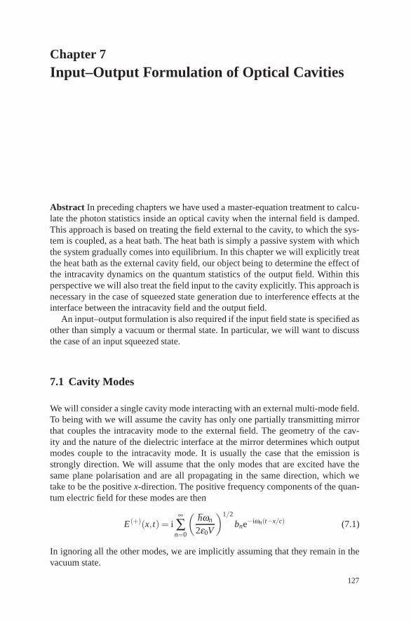
Chapter 7Input–Output Formulation of Optical Cavities
Abstract In preceding chapters we have used a master-equation treatment to calcu-late the photon statistics inside an optical cavity when the internal field is damped.This approach is based on treating the field external to the cavity, to which the sys-tem is coupled, as a heat bath. The heat bath is simply a passive system with whichthe system gradually comes into equilibrium. In this chapter we will explicitly treatthe heat bath as the external cavity field, our object being to determine the effect ofthe intracavity dynamics on the quantum statistics of the output field. Within thisperspective we will also treat the field input to the cavity explicitly. This approach isnecessary in the case of squeezed state generation due to interference effects at theinterface between the intracavity field and the output field.
An input–output formulation is also required if the input field state is specified asother than simply a vacuum or thermal state. In particular, we will want to discussthe case of an input squeezed state.
7.1 Cavity Modes
We will consider a single cavity mode interacting with an external multi-mode field.To being with we will assume the cavity has only one partially transmitting mirrorthat couples the intracavity mode to the external field. The geometry of the cav-ity and the nature of the dielectric interface at the mirror determines which outputmodes couple to the intracavity mode. It is usually the case that the emission isstrongly direction. We will assume that the only modes that are excited have thesame plane polarisation and are all propagating in the same direction, which wetake to be the positive x-direction. The positive frequency components of the quan-tum electric field for these modes are then
E(+)(x,t) = i∞
∑n=0
(hωn
2ε0V
)1/2
bne−iωn(t−x/c) (7.1)
In ignoring all the other modes, we are implicitly assuming that they remain in thevacuum state.
127
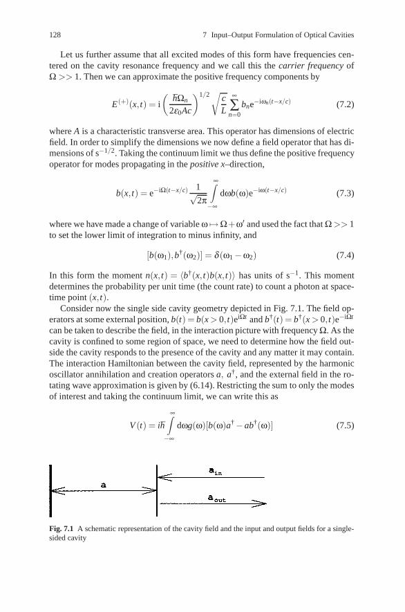
128 7 Input–Output Formulation of Optical Cavities
Let us further assume that all excited modes of this form have frequencies cen-tered on the cavity resonance frequency and we call this the carrier frequency ofΩ >> 1. Then we can approximate the positive frequency components by
E(+)(x,t) = i
(hΩn
2ε0Ac
)1/2√ cL
∞
∑n=0
bne−iωn(t−x/c) (7.2)
where A is a characteristic transverse area. This operator has dimensions of electricfield. In order to simplify the dimensions we now define a field operator that has di-mensions of s−1/2. Taking the continuum limit we thus define the positive frequencyoperator for modes propagating in the positive x–direction,
b(x,t) = e−iΩ(t−x/c) 1√2π
∞∫−∞
dωb(ω)e−iω(t−x/c) (7.3)
where we have made a change of variable ω �→Ω+ω′ and used the fact that Ω >> 1to set the lower limit of integration to minus infinity, and
[b(ω1),b†(ω2)] = δ (ω1−ω2) (7.4)
In this form the moment n(x,t) = 〈b†(x,t)b(x,t)〉 has units of s−1. This momentdetermines the probability per unit time (the count rate) to count a photon at space-time point (x,t).
Consider now the single side cavity geometry depicted in Fig. 7.1. The field op-erators at some external position, b(t) = b(x > 0,t)eiΩt and b†(t) = b†(x > 0,t)e−iΩt
can be taken to describe the field, in the interaction picture with frequency Ω. As thecavity is confined to some region of space, we need to determine how the field out-side the cavity responds to the presence of the cavity and any matter it may contain.The interaction Hamiltonian between the cavity field, represented by the harmonicoscillator annihilation and creation operators a, a†, and the external field in the ro-tating wave approximation is given by (6.14). Restricting the sum to only the modesof interest and taking the continuum limit, we can write this as
V (t) = ih
∞∫−∞
dωg(ω)[b(ω)a†−ab†(ω)] (7.5)
Fig. 7.1 A schematic representation of the cavity field and the input and output fields for a single-sided cavity

7.1 Cavity Modes 129
with [a,a†] = 1 and g(ω) is the coupling strength as a function of frequency whichis typically peaked around ω = 0 (which corresponds to ω = Ω in the original non-rotating frame). In fact g(ω) is the Fourier transform of a spatially varying couplingconstant that describes the local nature of the cavity/field interaction (see [1]). Ifthe cavity contains matter, the field inside the cavity may acquire some non trivialdynamics which then forces the external fields to have a time dependence differ-ent from the free field dynamics. This leads to an explicit time dependence in thefrequency space operators, b(t,ω), in the Heisenberg picture.
We now follow the approach of Collett and Gardiner [1]. The Heisenberg equa-tion of motion for b(t,ω), in the interaction picture, is
b(t,ω) =−iωb(ω)+ g(ω)a (7.6)
The solution to this equation can be written in two ways depending on weatherwe choose to solve in terms of the initial conditions at time t0 < t (the input) orin terms of the final conditions at times t1 > t, (the output). The two solutions arerespectively
b(t,ω) = e−iω(t−t0)b0(ω)+ g(ω)t∫
0
e−iω(t−t′)a(t ′)dt ′ (7.7)
where t0 < t and b0(ω) = b(t = t0,ω), and
b(t,ω) = e−iω(t−t1)b1(ω)−g(ω)t1∫
t
e−iω(t−t′)a(t ′)dt ′ (7.8)
where t < t1 and b1(ω) = b(t = t1,ω). In physical terms b0(ω) and b1(ω) are usuallyspecified at −∞ and +∞ respectively, that is, for times such that the field is simplya free field, however here we only require t0 < t < t1.
The cavity field operator obeys the equation
a =− ih[HS,a]−
∞∫−∞
dω g(ω)b(t,ω) (7.9)
where HS is the Hamiltonian for the cavity field alone. In terms of the solutionwith initial conditions, (7.7), this equation becomes
a =− ih[HS,a]−
∞∫−∞
dω g(ω)e−iω(t−t0)b0(ω)
−∞∫−∞
dω g(ω)2
t∫t0
e−iω(t−t′)a(t ′) (7.10)

130 7 Input–Output Formulation of Optical Cavities
We now assume that g(ω) is independent of frequency over a wide range of fre-quencies around ω = 0 (that is around ω = Ω in non rotating frame). This is the firstapproximation we need to get a Markov quantum stochastic process. Thus we set
g(ω)2 = γ/2π (7.11)
We also define an input field operator by
aIN(t) =− 12π
∞∫−∞
dωe−iω(t−t0)b0(ω) (7.12)
(the minus sign is a phase convention: left-going fields are negative, right-goingfields are positive). Using the relation
∞∫−∞
dωe−iω(t−t′) = 2πδ (t− t ′) (7.13)
the input field may be shown to satisfy the commutation relations
[aIN(t),a†IN(t ′) = δ (t− t ′) (7.14)
When (7.13) is achieved as the limit of an integral of a function which goes smoothlyto zero at ±∞ (for example, a Gaussian), the following result also holds
t∫t0
f (t ′)δ(t− t ′)dt ′ =t1∫
t
f (t ′)δ(t− t ′)dt ′ =12
f (t), (t0 < t < t1) (7.15)
Interchanging the order of time and frequency integration in the last term in (7.10)and using (7.15) gives
a(t) =− ih[a(t),HSYS]− γ
2a(t)+
√γaIN(t) (7.16)
Equation (7.16) is a quantum stochastic differential equation (qsde) for the intra-cavity field, a(t). The quantum noise term appears explicitly as the input field to thecavity.
In a similar manner we may substitute the solution in terms of final conditions,(7.8) into (7.10) to obtain the time-reversed qsde as
a(t) =− ih[a(t),HSYS]+
γ2
a(t)−√γaIN(t) (7.17)
where we define the output field operator as

7.2 Linear Systems 131
aOUT(t) =1√2π
∞∫−∞
dωe−iω(t−t1)b1(ω) (7.18)
(Note that the phase convention between left going and right going external fields re-quired for the boundary condition has been explicitly incorporated in the definitionsof aIN, aOUT). The input and output fields are then seen to be related by
aIN(t)+ aOUT(t) =√
γa(t) (7.19)
This represents a boundary condition relating each of the far field amplitudes outsidethe cavity to the internal cavity field. Interference terms between the input and thecavity field may contribute to the observed moments when measurements are madeon aOUT.
7.2 Linear Systems
For many systems of interest the Heisenberg equations of motion are linear and maybe written in the form
ddt
a(t) = Aa(t)− γ2
a(t)+√
γaIN(t) , (7.20)
where
a(t) =(
a(t)a†(t)
), (7.21)
aIN(t) =(
aIN(t)a†
IN(t)
), (7.22)
Define the Fourier components of the intracavity field by
a(t) =1√2π
∞∫−∞
e−iω(t−t0)a(ω)dω (7.23)
and a frequency component vector
a(ω) =(
a(ω)a†(ω)
)(7.24)
where a†(ω) is the Fourier transform of a†(t).The equations of motion become
[A+
(iω− γ
2
)1]
a(ω) =−√γaIN(ω) . (7.25)

132 7 Input–Output Formulation of Optical Cavities
However, we may use (7.18) to eliminate the internal modes to obtain
aOUT(ω) =−[A+
(iω +
γ2
)1][
A+(
iω− γ2
)1]−1
aIN(ω) . (7.26)
To illustrate the use of this result we shall apply it to the case of an empty one-sidedcavity. In this case the only source of loss in the cavity is through the mirror whichcouples the input and output fields. The system Hamiltonian is
HSYS = hω0a†a .
Thus
A =(−iω0 0
0 iω0
). (7.27)
Equation (7.26) then gives
aOUT(ω) =γ2 + i(ω−ω0)γ2 − i(ω−ω0)
aIN(ω) . (7.28)
Thus there is a frequency dependent phase shift between the output and input. Therelationship between the input and the internal field is
a(ω) =√γ
γ2 − i(ω−ω0)
aIN(ω) , (7.29)
which leads to a Lorentzian of width γ/2 for the intensity transmission function.
7.3 Two-Sided Cavity
A two-sided cavity has two partially transparent mirrors with associated loss coef-ficients γ1 and γ2, as shown in Fig. 7.2. In this case there are two input ports andtwo output ports. The equation of motion for the internal field is then given by anobvious generalisation as
da(t)dt
=−iω0a(t)− 12(γ1 + γ2)a(t)+
√γ1aIN(t)+
√γ2bIN(t) . (7.30)
Fig. 7.2 A schematic representation of the cavity field and the input and output fields for adouble-sided cavity

7.4 Two Time Correlation Functions 133
The relationship between the internal and input field frequency components for anempty cavity is then
a(ω) =√γ1aIN(ω)+
√γ2bIN(ω)( γ1+γ22
)− i(ω−ω0). (7.31)
The relationship between the input and output modes may be found using the bound-ary conditions at each mirror, see (7.19),
aOUT(t)+ aIN(t) =√
γ1a(t) , (7.32a)
bOUT(t)+ bIN(t) =√
γ2a(t) . (7.32b)
We find
aOUT(ω) =
[ γ1−γ22 + i(ω−ω0)
]aIN(ω)+
√γ1γ2bIN(ω)γ1+γ2
2 − i(ω−ω0)(7.33)
For equally reflecting mirrors γ1 = γ2 = γ this expression simplifies to
aOUT(ω) =i(ω−ω0)aIN(ω)+ γbIN(ω)
γ− i(ω−ω0). (7.34)
Near to resonance this is approximately a through pass Lorentzian filter
aOUT(ω)≈ γbIN(ω)γ− i(ω−ω0)
, (7.35)
This is only an approximate result, the neglected terms are needed to preservethe commutation relations. Away from resonance there is an increasing amount ofbackscatter. In the limit |ω−ω0| � γ the field is completely reflected
aOUT(ω) =−aIN(ω) . (7.36)
Before going on to consider interactions within the cavity we shall derive somegeneral relations connecting the two time correlation functions inside and outsidethe cavity.
7.4 Two Time Correlation Functions
Integrating (7.7) over ω , and using (7.13) gives
aIN(t) =√γ2
a(t)− 1√2π
∞∫−∞
dωb(ω ,t) . (7.37)

134 7 Input–Output Formulation of Optical Cavities
Let c(t) be any system operator. Then
[c(t),√
γaIN(t)] =γ2[c(t),a(t)] . (7.38)
Now since c(t) can only be a function of aIN(t ′) for earlier times t ′ < t and the inputfield operators must commute at different times we have
[c(t),√
γaIN(t ′)] = 0, t ′ > t . (7.39)
Similarly
[c(t),√
γaOUT(t ′)] = 0, t ′ < t . (7.40)
From (7.40 and 7.18) we may show that
[c(t),√
γaIN(t ′)] = γ[c(t),a(t)], t ′ < t . (7.41)
Combining (7.38–7.41) we then have
[c(t),√
γaIN(t ′)] = γ0(t− t ′)[c(t),a(t ′)] , (7.42)
where θ (t) is the step function
θ (t) =
⎧⎪⎨⎪⎩
1 t > 0,12 t = 0,
0 t < 0.
(7.43)
The commutator for the output field may now be calculated to be
[aOUT(t),a†OUT(t ′)] = [aIN(t),a†
IN(t ′)] (7.44)
as required.For the case of a coherent or vacuum input it is now possible to express vari-
ances of the output field entirely in terms of those of the internal system. Foran input field of this type all moments of the form 〈a†
IN(t)aIN(t ′)〉, 〈a(t)aIN(t ′)〉,〈a†(t)aIN(t ′)〉, 〈a†
IN(t)a(t ′)〉, and 〈a†IN(t)a†(t ′)〉 will factorise. Using (7.18) we find
〈a†OUT(t),aOUT(t ′)〉= γ〈a†(t),a(t ′)〉 , (7.45)
where〈U, V 〉 ≡ 〈U V 〉− 〈U〉〈V〉 . (7.46)
In this case there is a direct relationship between the two time correlation of theoutput field and the internal field. Consider now the phase dependent two time cor-relation function

7.5 Spectrum of Squeezing 135
〈aOUT(t),aOUT(t ′)〉= 〈aIN(t)−√γa(t),aIN(t ′)−√γa(t ′)〉= γ〈a(t),a(t ′)〉−√γ〈[aIN(t ′),a(t)]〉= γ〈a(t),a(t ′)〉+ γθ (t ′ − t)〈[a(t ′),a(t)]〉= γ〈a(max(t,t ′)),a(min(t,t ′))〉 . (7.47)
In this case the two time correlation functions of the output field are related to thetime ordered two time correlation functions of the cavity field.
These results mean that the usual spectrum of the output field, as given by theFourier transform of (7.45), will be identical to the spectrum of the cavity field. Thephoton statistics of the output field will also be the same as the intracavity field.Where a difference will arise, is in phase-sensitive spectrum such as in squeezingexperiments.
7.5 Spectrum of Squeezing
The output field from the cavity is a multi mode field. Phase-dependent propertiesof this field are measured by mixing the field, on a beam splitter, with a knowncoherent field – the local oscillator, as discussed in Sect. 3.8. The resulting fieldmay then be directed to a photodetector and the measured photocurrent directed tovarious devices such as a noise-power spectrum analyser to produce a spectrum,S(ω). If we write the signal field as aout(t) and the local oscillator is aLO(t), theaverage photo current is proportional to
i(t) = (1−η)〈a†LO(t)aLO(t)〉+
√η(1−η)〈aOUT(t)a†
LO(t)+ a†OUT(t)aLO(t)〉
+η〈a†OUT(t)aOUT(t)〉 (7.48)
If (1−η)〈a†LO(t)aLO(t)〉 >> η〈a†
OUT(t)aOUT(t)〉, we can neglect the last term in(7.48). If the local oscillator is in a coherent state 〈aLO(t)〉 = |β |eiθ e−iΩt , thennot only the average current, but all its moments are determined by the quantumstatistics of the quadrature phase operator
XOUTθ = aOUTe−i(θ−Ωt) + a†
OUTe−i(θ−Ωt) (7.49)
In particular, the noise power spectrum of the photocurrent is given by
S(ω,θ) =∫ ∞
−∞dt e−iωt〈: XOUT
θ (t),XOUTθ (0) :〉 (7.50)
where: indicates normal ordering. The combination aOUTeiΩt is simply the defini-tion of the output field in the interaction picture defined at frequency Ω. Using (7.47)and (7.49) this may be written in terms of the intracavity field as

136 7 Input–Output Formulation of Optical Cavities
S(ω,θ) = γ∫ ∞
−∞dt e−iωtT 〈: Xθ(t),Xθ(0) :〉 (7.51)
where T denotes time-ordering and Xθ(t) intracavity quadrature phase operator inan interaction picture at frequency, Ω, defined by the local oscillator frequency,
Xθ(t) = a(t)e−iθ + a†(t)eiθ (7.52)
Conventionally we define the in-phase and quadrature-phase operators as X1 =Xθ=0, X2 = Xθ=π/2.
7.6 Parametric Oscillator
We shall now proceed to calculate the squeezing spectrum from the output of aparametric oscillator. Below threshold the equations for the parametric oscillatorare linear and hence we can directly apply the linear operator techniques. Whenthe equations are nonlinear such as for the parametric oscillator above threshold,then linearization procedures must be used. One procedure using the Fokker–Planckequation is described in Chap. 8.
Below threshold the pump mode of the parametric oscillator may be treated clas-sically. It can then be described by the Hamiltonian
H = hωa†a +ih2
(εa†2− ε∗a2)+ aΓ† + a†Γ , (7.53)
where ε = εpχ and εp is the amplitude of the pump, and χ is proportional to the non-linear susceptibility of the medium. Γ is the reservoir operator representing cavitylosses. We consider here the case of a single ended cavity with loss rate γ1.
The Heisenberg equations of motion for a(t) are linear and given by (7.20) where
A =( γ1
2 −ε−ε∗ γ1
2
). (7.54)
We can obtain an expression for the Fourier components of the output fieldfrom (7.26)
aOUT(ω) =1[( γ1
2 − iω)2−|ε|2
]{[( γ1
2
)2+ ω2 + |ε|2
]
×aIN(ω)+ εγ1a†IN(−ω)
}. (7.55)
Defining the quadrature phase operators by
2aOUT = eiθ/2(XOUT1 + iXOUT
2 ) , (7.56)

7.6 Parametric Oscillator 137
where θ is the phase of the pump, we find the following correlations:
〈: XOUT1 (ω),XOUT
1 (ω ′) :〉= 2γ1|ε|( γ12 −|ε|
)2 + ω2δ (ω + ω ′) , (7.57)
〈: XOUT2 (ω),XOUT
2 (ω ′) :〉= −2γ1|ε|( γ12 + |ε|)2 + ω2
δ (ω + ω ′) , (7.58)
where the input field aIN has been taken to be in the vacuum.The δ function in (7.57 and 7.58) may be removed by integrating over ω ′ to give
the normally ordered spectrum: SOUT(ω):. The final result for the squeezing spectraof the quadrature is
SOUT1 (ω) = 1+ : SOUT
1 (ω) := 1 +2γ1|ε|( γ1
2 −|ε|)2 + ω2
, (7.59)
SOUT2 (ω) = 1+ : SOUT
2 (ω) := 1− 2γ1|ε|( γ12 + |ε|)2 + ω2
, (7.60)
These spectra are defined in a frame of frequency Ω so that ω = 0 is on cavityresonance.
The maximum squeezing occurs at the threshold for parametric oscillation |ε|=γ1/2 where
SOUT1 (ω) = 1 +
(γ1
ω
)2, (7.61)
SOUT2 (ω) = 1− γ2
1
γ21 + ω2
, (7.62)
Thus the squeezing occurs in the X2 quadrature which is π/2 out of phase with thepump. The light generated in parametric oscillation is therefore said to be phasesqueezed.
In Fig. 7.3 we plot SOUT2 (ω) at threshold. We see that at ω = 0, that is the cav-
ity resonance, the fluctuations in the X2 quadrature tend to zero. The fluctuations inthe X1 quadrature on the other hand diverge at ω = 0. This is characteristic of crit-ical fluctuations which diverge at a critical point. In this case however the critical
Fig. 7.3 A plot of the spec-trum of the squeezed quadra-ture for a cavity containing aparametric amplifier with aclassical pump. Solid: single-sided cavity with γ1 = γ2,dashed: double-sided cavity

138 7 Input–Output Formulation of Optical Cavities
flucuations are phase dependent. As the fluctuations in one phase are reduced to zerothe fluctuations in the other phase necessarily diverge. This characteristic of goodsqueezing near critical points is found in other phase dependent nonlinear opticalsystems [2]. This behaviour is in contrast to the threshold for laser oscillation wherethe critical fluctuations are random in phase.
7.7 Squeezing in the Total Field
The squeezing in the total field may be found by integrating (7.62) over ω . At thresh-old we find
STOT2 =
∫ (1− γ2
1
γ21 + ω2
)dω =
γ1
2. (7.63)
The squeezing in the total field is given by the equal time correlation functions
〈a,a〉OUT = γ1〈a,a〉,〈a,a†〉OUT = γ1〈a,a†〉 . (7.64)
Hence, the squeezing in the internal field is
V (X2) =12
. (7.65)
Thus the internal field mode is 50% squeezed, in agreement with the calculationsof Milburn and Walls [3]. This can be surpassed in the individual frequency compo-nents of the output field which have 100% squeezing for ω = 0. It is the squeezingin the individual frequency components of the output field which may be measuredby a spectrum analyser following a homodyne detection scheme.
7.8 Fokker–Planck Equation
We shall now give an alternative method for evaluating the squeezing spectrum. Thisconverts the operator master equation to a c-number Fokker–Planck equation. This isa useful technique when the operator equations are nonlinear. Standard linearizationtechniques for the fluctuations may be made in the Fokker–Planck equation. Weshall consider applications of this technique to nonlinear systems in Chap. 8.
We shall first demonstrate how time and normally-ordered moments may be cal-culated directly using the P representation. We consider the following time- andnormally-ordered moment

7.8 Fokker–Planck Equation 139
T 〈: X1(t)X1(0) :〉=e−2iθ 〈a(t)a(0)〉+ e2iθ〈a†(0)a†(t)〉+ 〈a†(t)a(0)〉+ 〈a†(0)a(t)〉 . (7.66)
The two-time correlation functions may be evaluated using the P representationwhich determines normally-ordered moments. Thus equal time moments of thec-number variables give the required normally-ordered operator moments. The twotime moments imply precisely the time ordering of the internal operators that arerequired to compute the output moments. This can be seen by noting that the evolu-tion of the system will in general mix a† and a. Hence a(t + τ) contains both a(t)and a†(t), τ > 0. In a normally-ordered two time product a(t + τ) must thereforestand to the left of a(t), similarly a†(t + τ) must stand to the right of a†(t). Thus
〈α(t + τ)α(t)〉p = 〈a(t + τ)a(t)〉 , (7.67)
〈α∗(t + τ)α∗(t)〉p = 〈a†(t)a†(t + τ)〉 , (7.68)
where the left-hand side of these equations represent averages of c-number vari-ables over the P representation. The normally-ordered output correlation matrix de-fined by
: COUT(τ) :=(〈aOUT(t + τ),aOUT(t)〉 〈a†
OUT(t),aOUT(t + τ)〉〈a†
OUT(t + τ),aOUT(t)〉 〈a†OUT(t + τ),a†
OUT(t)〉)
(7.69)
is given by
: COUT(τ) : = γ( 〈α(t + τ),α(t)〉 〈α(t + τ),α∗(t)〉〈α∗(t + τ),α(t)〉 〈α∗(t + τ),α∗(t)〉
)
≡ γCp(τ) . (7.70)
The two time correlation functions for the output field may be calculated directlyfrom the correlation functions of the stochastic variables describing the internal fieldusing the P representation.
For nonlinear optical processes the Fokker–Planck equation for the P functionmay have nonlinear drift terms and nonconstant diffusion. In such circumstanceswe first linearise the equation about the deterministic steady states, to obtain a linearFokker–Planck equation of the form
∂P∂ t
(α) =(
∂∂αi
Aiαi +12
∂ 2
∂αi∂α jDi j
)P(α) , (7.71)
where A is the drift matrix, and D is the diffusion matrix. The linearised descrip-tion is expected to give the correct descriptions away from instabilities in the de-terministic equations of motion. For fields exhibiting quantum behaviour, such assqueezing, D is non-positive definite and a Fokker–Planck equation is not definedfor the Glauber–Sudarshan P function. In these cases a Fokker–Planck equation is

140 7 Input–Output Formulation of Optical Cavities
defined for the positive P representation, where α∗ is replaced by α† an independentcomplex variable as described in Chap. 6.
The spectral matrix S(ω) is defined as the Fourier transform of Cp(τ). In a lin-earised analysis it is given by
S(ω) = γ(A+ iωI)−1D(AT − iωI)−1 . (7.72)
The squeezing spectrum for each quadrature phase is then given by
: SOUT1 (ω) := γ[e−2iθS11(ω)+ e2iθS22(ω)+ S12(ω)+ S21(ω)] (7.73)
: SOUT2 (ω) := γ[−e−2iθS11(ω)− e2iθS22(ω)+ S12(ω)+ S21(ω)] (7.74)
These spectra are defined in a frame of frequency Ω (the cavity-resonance fre-quency) so that ω = 0 corresponds to the cavity resonance.
It should be noted that in the above derivation there is only one input field and oneoutput field, that is, there is only one source of cavity loss. Thus the above resultsonly apply to a single-ended cavity; one in which losses accrue only at one mirror.
If there are other significant losses from the cavity the γ appearing in (7.60 and7.61) is not the total loss but only the loss from the mirror through which the outputfield of interest is transmitted.
The above procedure enables one to calculate the squeezing in the output fieldfrom an optical cavity, provided the internal field may be described by the linearFokker–Planck equation (7.71).
Alternatively the squeezing spectrum for the parametric oscillator may be calcu-lated using the Fokker–Planck equation. The Fokker–Planck equation for the dis-tribution P(α) for the system described by the Hamiltonian (7.53) may be derivedusing the techniques of Chap. 6.
∂P(α)∂ t
=−{(
ε∗∂
∂α∗α + ε
∂∂α
α∗)
+γ1
2
(∂
∂α∗α∗+
∂∂α
α)
+12
[ε∗
∂ 2
∂α∗2+ ε
∂ 2
∂α2
]}P(α) (7.75)
The drift and diffusion matrices are
A =( γ1
2 −ε−ε∗ γ1
2
), D =
(ε 00 ε∗
). (7.76)
Direct application of (7.72–7.74) yields the squeezing spectra given by (7.59 and7.60).

Further Reading 141
Exercises
7.1 Calculate the squeezing spectrum for a degenerate parametric oscillator withlosses γ1 and γ2 at the end mirrors.
7.2 Calculate the squeezing spectrum for a non-degenerate parametric oscillator.[Hint: Use the quadratures for a two mode system described in (5.49)].
References
1. W. Gardiner, IBM J. Res. Dev. 32, 127 (1988); M.J. Collett and C.W. Gardiner, Phys. Rev. 30,1386 (1984)
2. M.J. Collett, D.F. Walls: Phys. Rev A 32 2887 (1985)3. G.J. Milburn, D.F. Walls: Optics Commun. 39, 401 (1981)
Further Reading
Gardiner, C.W.: Quantum Noise (Springer, Berlin, Heidelberg 1991)Reynaud, S.: A. Heidman: Optics Comm. 71, 209 (1989)Yurke, B.: Phys. Rev. A 32, 300 (1985)

Chapter 8Generation and Applications of Squeezed Light
Abstract In this chapter we shall describe how the squeezing spectrum may be cal-culated for intracavity nonlinear optical processes. We shall confine the examples toprocesses described by an effective Hamiltonian where the medium is treated clas-sically. We are able to extend the treatment o squeezing in the parametric oscillatorto the above threshold regime. In addition, we calculate the squeezing spectrum forsecond harmonic generation and dispersive optical bistability. We also consider thenon degenerate parametric oscillator where it is possible to achieve intensity fluctu-ations below the shot-noise level for the difference in the signal and idle intensities.Two applications of squeezed light will be discussed: interferometric detection ofgravitational radiation and sub-shot-noise phase measurements.
8.1 Parametric Oscillation and Second Harmonic Generation
We consider the interaction of a light mode at frequency ω1 with its second har-monic at frequency 2ω1. The nonlinear medium is placed within a Fabry–Perot cav-ity driven coherently either at frequency 2ω1 (parametric oscillation or frequencyω1 (second harmonic generation)). We shall begin by including driving fields bothat frequency ω1 and 2ω1 so that both situations may be described within the oneformalism. We write the Hamiltonian as [1]
H = H1 +H2 ,
H1 = �ω1a†1a1 + 2hω1a†
2a2 + ihκ2
(a†21 a2−a2
1a†2)+ ih(E1a†
1 e−iω1t)
−E∗1a1eiω1t)+ ih(E2a†2e−2iω1t −E∗2a2e2iω1t) ,
H2 = a1Γ†1 + a†
1Γ1 + a2Γ†2 + a†
2Γ2 ,
where a1 and a2 are the Boson operators for modes of frequency ω1 and 2ω1, re-spectively, κ is the coupling constant for the interaction between the two modes and
143

144 8 Generation and Applications of Squeezed Light
the spatial mode functions are chosen so that κ is real, Γ1, Γ2 are heat bath operatorswhich represent cavity losses for the two modes and E1 and E2 are proportional tothe coherent driving field amplitudes.
The master equation for the density operator of the two cavity modes after tracingout over the reservoirs is
∂ρ∂ t
=1ih
[H1, ρ ]+ (L1 + L2)ρ , (8.2)
where
Liρ = γi(2aiρa†i −a†
i aiρ−ρa†i ai) ,
and γi are the cavity damping rates of the modes.This master equation may be converted to a c-number Fokker–Planck equation
in the generalised P representation. The generalised P representation must be usedsince the c-number equation would have a non-positive definite diffusion matrix ifthe Glauber–Sudarshan P representation were used. The result is
∂∂ t
P(a) =
{∂
∂α1(γ1α1−E1−κα†
1 α2)+∂
∂α†1
(γ1α†1 −E∗1 −κα1α†
2 )
+∂
∂α2
(γ2α2−E2 +
κ2
α21
)+
∂∂α†
2
(γ2α†
2 −E∗2 +κ2
α†21
)
+12
[∂ 2
∂α21
(κα2)+∂ 2
∂α†21
(κα†2 )
]}P(a) , (8.3)
where a = [α1, α†1 , α2, α†
2 ], and we have made the following transformation to therotating frames of the driving fields
α1→ α1 exp(−iω1t), α2→ α2 exp(−2iω1t) .
In the generalized P representation α and α† are independent complex variablesand the Fokker–Planck equation has a positive semi-definite diffusion matrix in aneight-dimensional space. This allows us to define equivalent stochastic differentialequations using the Ito rules
∂∂ t
(α1
α†1
)=(
E1 + κα†1 α2− γ1α1
E∗1 + κα1α†2 − γ1α†
1
)+(
κα2 00 κα†
2
)1/2(η1(t)η†
1 (t)
), (8.4)
∂∂ t
(α2
α†2
)=(
E2− κ2 α2
1 − γ2α2
E∗2 − κ2 α†2
1 − γ2α†2
), (8.5)
where η1(t), η†1 (t) are delta correlated stochastic forces with zero mean, namely

8.1 Parametric Oscillation and Second Harmonic Generation 145
〈η1(t)〉= 0
〈η1(t)η1(t′)〉= δ(t− t ′) (8.6)
〈η1(t)η†(t ′)〉= 0 .
8.1.1 Semi-Classical Steady States and Stability Analysis
The semi-classical or mean value equations follow directly from (8.4 and 8.5) withthe replacement of α†
i by α∗i .
∂∂ t
α1 = E1 + κα∗1 α2− γ1α1 , (8.7)
∂α2
∂ t= E2 +
κ2
α21 − γ2α2 . (8.8)
We shall investigate the steady states of these equations and their stability. The sta-bility of the steady states may be determined by a linearized analysis for small per-turbations around the steady state
α1 = α01 + δα1 , α2 = α0
2 + δα2 , (8.9)
where α01 , α0
2 are the steady-state solutions of (8.7 and 8.8). The linearized equa-tions for the fluctuations are
∂∂ t
⎛⎜⎜⎝
δα1
δα∗1δα2
δα∗2
⎞⎟⎟⎠=
⎛⎜⎜⎝−γ1 κα0
2 κα01 0
κα0∗2 −γ1 0 κα0
1−κα0∗
1 0 −γ2 00 −κα0∗
1 0 −γ2
⎞⎟⎟⎠
⎛⎜⎜⎝
δα1
δα∗1δα2
δα∗2
⎞⎟⎟⎠ . (8.10)
The four eigenvalues of these equations are
λ1, λ2 =−12(−|κα0
2 |+ γ1 + γ2)± 12[(−|κα0
2 |+ γ1− γ2)2−4|κα01 |2]1/2 ,
λ3, λ4 =−12(|κα0
2 |+ γ1 + γ2)± 12[(|κα0
2 |+ γ1− γ2)2−4|κα01 |2]1/2 . (8.11)
The fixed points become unstable when one or more of these eigenvalues has apositive real part. If a fixed point changes its stability as one of the parameters isvaried we call this a bifurcation. In this problem the nature of bifurcations exhibitedcome in many forms including a fixed point to limit cycle transition.
We shall consider the cases of parametric oscillation and second harmonicgeneration separately.

146 8 Generation and Applications of Squeezed Light
Fig. 8.1 Steady state ampli-tude of the fundamental modeversus pump field amplitudefor parametric oscillation,κ = 1.0, Ec
2 = 4.0
8.1.2 Parametric Oscillation
For parametric oscillation only the mode at frequency 2ω1 is pumped so we set E1 =0. The stable steady state solutions for the mode amplitudes are below thresholdE2 < Ec
2
α01 = 0, α0
2 =E2
γ2, (8.12)
above threshold E2 > Ec2
α01 =±
[2κ
(E2−Ec2)]1/2
, α02 =
γ1
κ, (8.13)
where Ec2 = γ1γ2/κ , and we have taken E2 to be positive. Thus the system exhibits
behaviour analogous to a second-order phase transition at E2 = Ec2 where the below-
threshold solution α01 = 0 becomes unstable and the system moves onto a new stable
branch. Above threshold there exist two solutions with equal amplitude and oppositephase. In Fig. 8.1 we plot the amplitude α0
1 versus E2.
8.1.3 Second Harmonic Generation
For second harmonic generation only the cavity mode at frequency ω is pumpedso we set E2 = 0. Equations (8.7 and 8.8) then yield the following equation for thesteady state amplitude of the second harmonic
−2γ2(κα02 )3 + 4γ1γ2(κα0
2 )−2γ21 γ2(κα0
2 ) = |κE1|2 . (8.14)
This gives a solution for α02 which is negative and the intensity |α0
2 |2 is a monoton-ically increasing, single valued function of |E1|2.
However from the stability analysis we find that the eigenvalues
λ1, λ2→ 0± iω , (8.15)
where ω = [γ2(2γ1 + γ2)]1/2 when the driving field E1 reaches the critical value
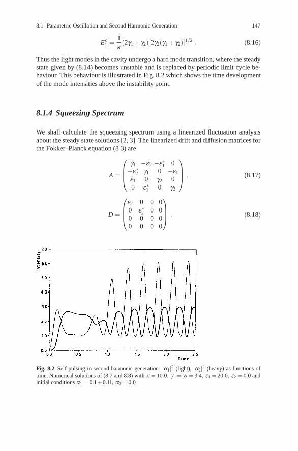
8.1 Parametric Oscillation and Second Harmonic Generation 147
Ec1 =
1κ
(2γ1 + γ2)[2γ2(γ1 + γ2)]1/2 . (8.16)
Thus the light modes in the cavity undergo a hard mode transition, where the steadystate given by (8.14) becomes unstable and is replaced by periodic limit cycle be-haviour. This behaviour is illustrated in Fig. 8.2 which shows the time developmentof the mode intensities above the instability point.
8.1.4 Squeezing Spectrum
We shall calculate the squeezing spectrum using a linearized fluctuation analysisabout the steady state solutions [2, 3]. The linearized drift and diffusion matrices forthe Fokker–Planck equation (8.3) are
A =
⎛⎜⎜⎝
γ1 −ε2 −ε∗1 0−ε∗2 γ1 0 −ε1
ε1 0 γ2 00 ε∗1 0 γ2
⎞⎟⎟⎠ , (8.17)
D =
⎛⎜⎜⎝
ε2 0 0 00 ε∗2 0 00 0 0 00 0 0 0
⎞⎟⎟⎠ . (8.18)
Fig. 8.2 Self pulsing in second harmonic generation: |α1|2 (light), |α2|2 (heavy) as functions oftime. Numerical solutions of (8.7 and 8.8) with κ = 10.0, γ1 = γ2 = 3.4, ε1 = 20.0, ε2 = 0.0 andinitial conditions α1 = 0.1+0.1i, α2 = 0.0
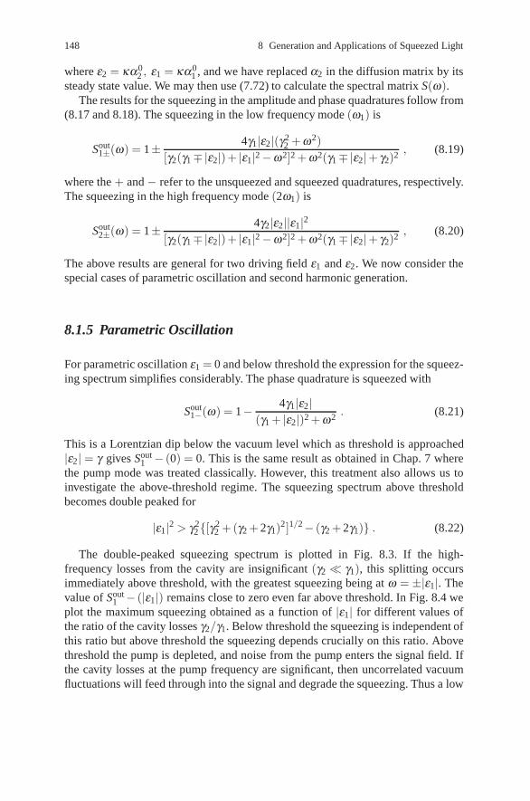
148 8 Generation and Applications of Squeezed Light
where ε2 = κα02 , ε1 = κα0
1 , and we have replaced α2 in the diffusion matrix by itssteady state value. We may then use (7.72) to calculate the spectral matrix S(ω).
The results for the squeezing in the amplitude and phase quadratures follow from(8.17 and 8.18). The squeezing in the low frequency mode (ω1) is
Sout1±(ω) = 1± 4γ1|ε2|(γ2
2 + ω2)[γ2(γ1∓|ε2|)+ |ε1|2−ω2]2 + ω2(γ1∓|ε2|+ γ2)2 , (8.19)
where the + and − refer to the unsqueezed and squeezed quadratures, respectively.The squeezing in the high frequency mode (2ω1) is
Sout2±(ω) = 1± 4γ2|ε2||ε1|2
[γ2(γ1∓|ε2|)+ |ε1|2−ω2]2 + ω2(γ1∓|ε2|+ γ2)2 , (8.20)
The above results are general for two driving field ε1 and ε2. We now consider thespecial cases of parametric oscillation and second harmonic generation.
8.1.5 Parametric Oscillation
For parametric oscillation ε1 = 0 and below threshold the expression for the squeez-ing spectrum simplifies considerably. The phase quadrature is squeezed with
Sout1−(ω) = 1− 4γ1|ε2|
(γ1 + |ε2|)2 + ω2 . (8.21)
This is a Lorentzian dip below the vacuum level which as threshold is approached|ε2| = γ gives Sout
1 − (0) = 0. This is the same result as obtained in Chap. 7 wherethe pump mode was treated classically. However, this treatment also allows us toinvestigate the above-threshold regime. The squeezing spectrum above thresholdbecomes double peaked for
|ε1|2 > γ22{[γ2
2 +(γ2 + 2γ1)2]1/2− (γ2 + 2γ1)} . (8.22)
The double-peaked squeezing spectrum is plotted in Fig. 8.3. If the high-frequency losses from the cavity are insignificant (γ2 � γ1), this splitting occursimmediately above threshold, with the greatest squeezing being at ω = ±|ε1|. Thevalue of Sout
1 − (|ε1|) remains close to zero even far above threshold. In Fig. 8.4 weplot the maximum squeezing obtained as a function of |ε1| for different values ofthe ratio of the cavity losses γ2/γ1. Below threshold the squeezing is independent ofthis ratio but above threshold the squeezing depends crucially on this ratio. Abovethreshold the pump is depleted, and noise from the pump enters the signal field. Ifthe cavity losses at the pump frequency are significant, then uncorrelated vacuumfluctuations will feed through into the signal and degrade the squeezing. Thus a low

8.1 Parametric Oscillation and Second Harmonic Generation 149
Fig. 8.3 The squeezing spec-trum for parametric oscilla-tion with γ1 = 2γ2. Solid line:on threshold with ε2 = γ1.Dashed line: above thresholdwith ε1 = γ2
cavity loss at the pump frequency by comparison with the signal loss is needed toobtain good squeezing above threshold in the parametric oscillator.
We may also consider the squeezing in the pump mode. Below threshold thismode is not squeezed. Above threshold the peak squeezing (at ω = 0) increases toa maximum value of 50% at |ε1| = 2γ1γ2. When |ε1| = 2γ2
1 + 12 γ2
2 , we again find asplitting into a double peak.
8.1.6 Experiments
The first experiment to demonstrate the generation of squeezed light in an opticalparametric oscillator below threshold was been performed by Wu et al. [4]. Theydemonstrated reductions in photocurrent noise greater than 60% (4 dB) below thelimit set by the vacuum fluctuations of the field are observed in a balanced ho-modyne detector. Lam et al. [5] reported 7 dB of measured vacuum squeezing. Aschematic of their experiment is shown in Fig. 8.5. The experiment used a mono-lithic MgO:LiNbO3 nonlinear crystal as the nonlinear medium. This was pumpedat a wavelength of 532 nm from a second harmonic source (a hemilithic crystal ofMgO:LiNbO3). Squeezed light is generated at 1064nm. The squeezing cavity out-put coupler is 4% reflective to 532 nm and 95.6% reflective to 1064 nm. The otherend is a high reflector with 99.96% for both wavelengths. The cavity finesse wasF = 136, and a free spectral range FSR = 9GHz. The cavity linewidth was 67 MHz.The output of the OPO is directed to a pure TEM00 mode cleaning cavity with a
Fig. 8.4 Maximum squeezingabove threshold as a func-tion of the amplitude of thefundamental mode |ε1|, fordifferent values of the cavitylosses γ2/γ1; (a) 0.02, (b) 0.1,(c) 1.0
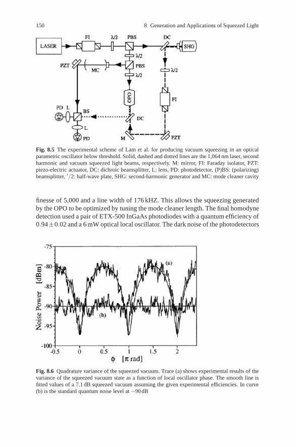
150 8 Generation and Applications of Squeezed Light
Fig. 8.5 The experimental scheme of Lam et al. for producing vacuum squeezing in an opticalparametric oscillator below threshold. Solid, dashed and dotted lines are the 1,064 nm laser, secondharmonic and vacuum squeezed light beams, respectively. M: mirror, FI: Faraday isolator, PZT:piezo-electric actuator, DC: dichroic beamsplitter, L: lens, PD: photodetector, (P)BS: (polarizing)beamsplitter, ′/2: half-wave plate, SHG: second-harmonic generator and MC: mode cleaner cavity
finesse of 5,000 and a line width of 176 kHZ. This allows the squeezing generatedby the OPO to be optimized by tuning the mode cleaner length. The final homodynedetection used a pair of ETX-500 InGaAs photodiodes with a quantum efficiency of0.94±0.02 and a 6 mW optical local oscillator. The dark noise of the photodetectors
Fig. 8.6 Quadrature variance of the squeezed vacuum. Trace (a) shows experimental results of thevariance of the squeezed vacuum state as a function of local oscillator phase. The smooth line isfitted values of a 7.1 dB squeezed vacuum assuming the given experimental efficiencies. In curve(b) is the standard quantum noise level at −90dB

8.2 Twin Beam Generation and Intensity Correlations 151
from OPO
coherent input
EOM
i(t)
λ gain
Fig. 8.7 An electro-optic feed-forward scheme used by Lam et al. to produce a bright squeezedstate. The electro-optic modulator (EOM) is controlled be the photo-current i(t)
was 10 dB below the measured vacuum quantum noise level and hence the squeezedvacuum measurement does not require any electronic noise floor correction.
In Fig. 8.6 are the results of Lam et al. At a pump power of around 60± 10%,they found an optimal vacuum squeezing of more than 7.0±0.2dB.
In some applications it is desirable to have a squeezed stater with a non zerocoherent amplitude, a bright squeezed state. The conventional way to do this wouldbe to simply mix the squeezed vacuum state produced by the OPO with a coherentstate on a beam splitter (see Exercise 8.1). However the transmitivity of the squeezedvacuum state must be very close to unity in order not to loose the squeezing. Thismeans that very little of the coherent light is reflected and the scheme is ratherwasteful of power. Lam et al. also showed two alternative methods to produce asqueezed state with a significant coherent amplitude. In the first method a small seedcoherent beam was injected into the back face of the OPO. This gave an amplitudesqueezed state with 4 dB of squeezing. The second method was based on electro-optical feed-forward to transfer the squeezing onto a coherent beam, see Fig. 8.7.By carefully adjusting the gain on the controlling photon current to the EOM abright squeezed beam with squeezing in the amplitude quadrature corresponding toa reduction of intensity noise of 4db below shot noise.
8.2 Twin Beam Generation and Intensity Correlations
Another second-order process which can produce non-classical states isnon-degenerate down conversion. A pump photon with frequency 2ω creates asignal and an idler photon each with frequency ω but different polarisations.

152 8 Generation and Applications of Squeezed Light
Alternatively the signal and idler may be distinguished by having different frequen-cies ω1 and ω2, respectively, such that ω1 + ω2 = 2ω . Such a process ensures thatthe photon numbers in the signal and idler beams are highly correlated. Althoughthe intensity of each beam may fluctuate, the fluctuations on the two beams areidentical. This suggests that the intensity difference of the two beams will carry nofluctuations at all. That is to say, the variance of I1− I2 can be zero. If the process oc-curs inside a cavity the correlation between the two photons may be lost as photonsescape the cavity. This is true for times short compared to the cavity lifetime. Forlong times, however, the correlation is restored; if one waits long enough all photonswill exit the cavity. Consequently the spectrum of fluctuations in the difference ofthe intensities in the two beams reduces to zero at zero frequency.
The Hamiltonian describing this process may be written as
HI = ihχ(a0a†1a†
2−a†0a1a2) , (8.23)
where a0 describes the pump field, while a1 and a2 describe the signal and idlerfields. The pump field is driven by a coherent field external to the cavity with ampli-tude ε . The damping rates for the three cavity modes a0, a1 and a2 are κ0, κ1 andκ2, respectively.
Following from the Fokker–Planck equation for the positive P representation weestablish the c-number stochastic differential equations [6]
α0 =−κ0α0 + ε− χα1α2 ,
α1 =−κ1α1 + χα0α†2 + R1(t) ,
α2 =−κ2α2 + χα0α†1 + R2(t) . (8.24)
In our treatment we will assume for simplicity that κ1 = κ2 = κ , where the onlynon-zero noise correlation functions are
〈R1(t)R2(t ′)〉= χ〈α0〉δ (t− t ′),
〈R†1(t)R
†2(t′)〉= χ〈α†
0 〉δ (t− t ′) . (8.25)
The semi-classical steady state solutions depend on whether the driving field ε isabove or below a critical “threshold” value given by
εthr =κ0κχ
. (8.26)
Above threshold one of the eigenvalues of the drift matrix is zero. This is associatedwith a phase instability. To see this we use an amplitude and phase representation:
α j(t) = r j[1 + μ j(t)]e−i(φ j+ψ j(t)) (8.27)
where r j,φ j are the steady state solutions, and μ j(t) and ψ j(t) represent small fluctu-ations around the steady state. Solving for the steady state below threshold we have

8.2 Twin Beam Generation and Intensity Correlations 153
r1 = r2 = 0, r0 =|ε|κ0
, φ0 = φp , (8.28)
where we have used ε = |ε|eiφp, with φp denoting the phase of the coherent pump.Above threshold
r0 =κχ
, φ0 = φp ,
r1 = r2 =√
κ0κχ
(E−1)1/2 , φ1 + φ2 = φp , (8.29)
with
E =|ε||εthr| . (8.30)
Note that in the above threshold solution only the sum of the signal and idler phasesis defined. No steady state exists for the phase difference. It is the phase differencevariable which is associated with the zero eigenvalue.
We now turn to an analysis of the intensity fluctuations above threshold. Thenonlinear dynamics of (8.24) is approximated by a linear dynamics for intensityfluctuations about the steady states above threshold. Define the new variables by
ΔI j = α†j α j− Iss
j , (8.31)
where Issj is the steady state intensity above threshold for each of the three modes.
It is more convenient to work with scaled “intensity-sum” and ‘intensity-difference’variables defined by
ΔIs = κ(ΔI1 + ΔI2), ΔID = κ(ΔI1−ΔI2) , (8.32)
The linear stochastic differential equations are then given by
ΔI0 =−κ0ΔI0−ΔIs , (8.33)
ΔIs = 2κκ0(E−1)ΔI0 + Fs(t) , (8.34)
ΔID =−2κΔID + FD(t) , (8.35)
where the non zero noise correlations are
〈Fs(t)Fs(t ′)〉=−〈FD(t)FD(t ′)〉= 4κ0κ4
χ2 (E−1)δ (t− t ′) . (8.36)
We are now in a position to calculate the spectrum of fluctuations in the intensitydifference in the signal and idler modes outside the cavity. The equation for theintensity difference fluctuations may be solved immediately to give
ΔI0(t) = ΔID(0)e−2κt +t∫
0
dt ′e−2κ(t−t′)FD(t ′) . (8.37)

154 8 Generation and Applications of Squeezed Light
Thus the steady state two-time correlation function is found to be
〈ID(τ) , ID(0)〉= 〈ΔID(τ)ΔID(0)〉= κ0κ3
χ2 (E−1)e−2κτ (8.38)
with 〈A,B〉= 〈AB〉− 〈A〉〈B〉.The spectrum of fluctuations in the intensity difference field outside the cavity is
defined by
SD(ω) =∫
dτe−iωτ〈I1(τ)− I2(τ), I1(0)− I2(0)〉ss , (8.39)
where I j(t) are the external intensity operators. However, from Chap. 7, we canrelate this operator average to the c-number averages for α j(t) inside the cavity. Theresult is
〈I j(τ), Ik(0)〉= 2δ jkκδ (τ)〈I j(0)〉+ 4κ2〈I j(τ), Ik(0)〉 , (8.40)
where I j ≡ α†j (t)α j(t). Finally, we write the result directly in terms of the valuables
ΔID(t),
SD(ω) = S0 + 4∫
dτe−iωτ〈ΔID(τ)ΔID(0)〉 , (8.41)
where
S0 = 2κ(〈I1〉ss + 〈I2〉ss) =4κ0κ3
χ2 (E−1) . (8.42)
The frequency independent term S0 represents the contribution of the shot-noisefrom each beam. Thus to quantify the degree of reduction below the shot-noiselevel we define the ‘normalised’ intensity difference spectrum
SD(ω)≡ SD(ω)S0
. (8.43)
Substituting (8.38 and 8.42) into (8.41), and integrating we obtain
SD(ω)≡ ω2
ω2 + 4κ2 . (8.44)
This is a simple inverted Lorentzian with a width 2κ . As expected, at zero frequencythere is perfect noise suppression in the intensity difference between the signal andidler. This result was first obtained by Reynaud et al. [7].
The above results assume no additional cavity losses beyond those correspond-ing to the (equal) transmitivities at the output mirror. When additional losses areincluded the correlation between the signal and idler is no longer perfect as one ofthe pair of photons may be lost otherwise than through the output mirror. In thatcase there is no longer perfect suppression of quantum noise at zero frequency [8].The result is shown in Fig. 8.8a. Furthermore, the spectrum of intensity differencefluctuations is very sensitive to any asymmetry in the loss for each mode [8]. InFig. 8.8b we depict the effect of introducing different intracavity absorption rates

8.2 Twin Beam Generation and Intensity Correlations 155
Fig. 8.8 The effect of intracavity absorption on the intensity difference spectrum. (a) A plot of thenormalized spectrum when the total cavity losses for each mode are equal to the total loss from thepump mode, and greater than the output loss rate κ (solid line). The dashed line shows the perfectcase when the only losses are through the output mirrors. (b) The effect of asymmetrical intracavityabsorption. The total loss for the idler is equal to the idler damping rate but the damping rate forthe signal is only 80% of the total loss for that mode. E = 1.05 solid line, E = 2.0, dashed line. [8]
for each mode. This phenomenon could form the basis of a sub-shot-noise absorp-tion spectrometer.
The prediction of noise suppression in the differenced intensity has been con-firmed in the experiment of Heidmann et al. [9]. They used a type II phase-matchedpotassium triphosphate, known as KTP, crystal placed inside an optical cavity, thusforming an Optical Parametric Oscillator (OPO).
The damping constant at the pump frequency was much greater than for the sig-nal and idler. Above threshold the OPO emits two cross polarised twin beams at ap-proximately the same frequency. The twin beams are separated by polarising beamsplitters and then focussed on two photodiodes which have quantum efficiencies of90%. The two photo-currents are amplified and then subtracted with a 180◦ powercombiner. The noise on the resulting difference current is then monitored by a spec-trum analyser.
A maximum noise reduction of 30%±5% is observed at a frequency of 8 MHz.The noise reduction is better than 15% from 3 to 13 MHz. The noise reduction islimited due to other losses inside the OPO and various detector inefficiencies.
Using an α-cut KTP crystal, Gao et al. [10] achieved a noise reduction in theintensity difference of 88% below the shot noise level, corresponding to a 9.2 dBreduction. They also showed how such highly correlated intensities could be usedto enhance the signal-to-noise ratio for relative absorption measurements when onebeam passes through an absorber. The improvement was about 7 dB.
The bandwidth of squeezing in cavity experiments is restricted to the cavity band-width. Single-pass experiments are feasible using the higher intensity possible withpulsed light. Pulsed twin beams of light have been generated by means of an opticalparametric amplifier that is pumped by the second harmonic of a mode-locked andQ-switched Nd : YAG laser [11]. While the noise levels of the individual signal andidler beams exceed their coherent state limits by about 11 dB the correlation is sostrong that the noise in the difference current falls below the quantum limit by morethan 6 dB (75%).
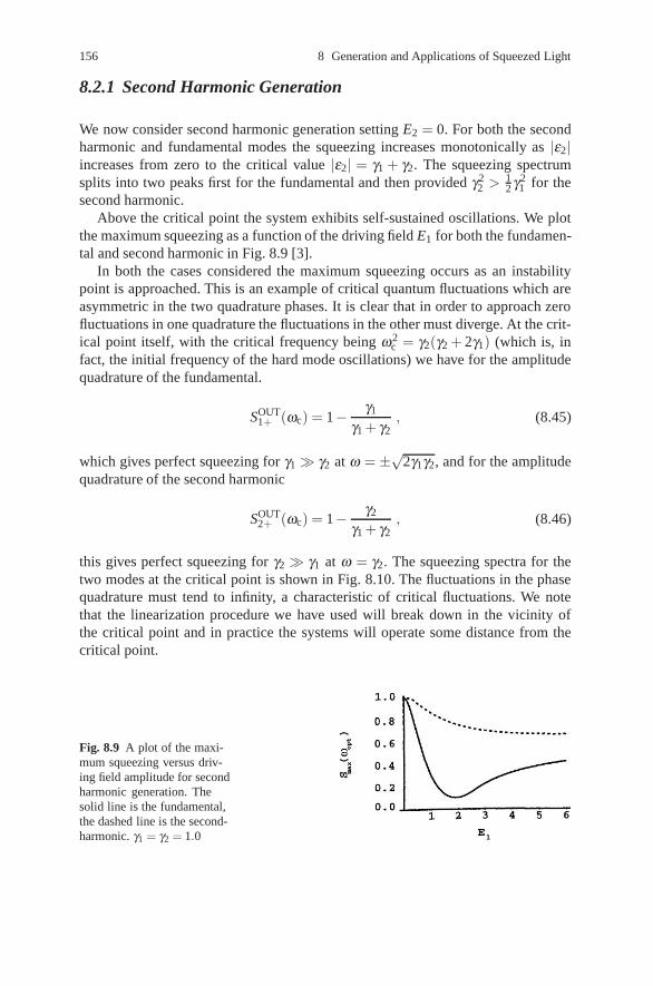
156 8 Generation and Applications of Squeezed Light
8.2.1 Second Harmonic Generation
We now consider second harmonic generation setting E2 = 0. For both the secondharmonic and fundamental modes the squeezing increases monotonically as |ε2|increases from zero to the critical value |ε2| = γ1 + γ2. The squeezing spectrumsplits into two peaks first for the fundamental and then provided γ2
2 > 12 γ2
1 for thesecond harmonic.
Above the critical point the system exhibits self-sustained oscillations. We plotthe maximum squeezing as a function of the driving field E1 for both the fundamen-tal and second harmonic in Fig. 8.9 [3].
In both the cases considered the maximum squeezing occurs as an instabilitypoint is approached. This is an example of critical quantum fluctuations which areasymmetric in the two quadrature phases. It is clear that in order to approach zerofluctuations in one quadrature the fluctuations in the other must diverge. At the crit-ical point itself, with the critical frequency being ω2
c = γ2(γ2 + 2γ1) (which is, infact, the initial frequency of the hard mode oscillations) we have for the amplitudequadrature of the fundamental.
SOUT1+ (ωc) = 1− γ1
γ1 + γ2, (8.45)
which gives perfect squeezing for γ1� γ2 at ω = ±√2γ1γ2, and for the amplitudequadrature of the second harmonic
SOUT2+ (ωc) = 1− γ2
γ1 + γ2, (8.46)
this gives perfect squeezing for γ2 � γ1 at ω = γ2. The squeezing spectra for thetwo modes at the critical point is shown in Fig. 8.10. The fluctuations in the phasequadrature must tend to infinity, a characteristic of critical fluctuations. We notethat the linearization procedure we have used will break down in the vicinity ofthe critical point and in practice the systems will operate some distance from thecritical point.
Fig. 8.9 A plot of the maxi-mum squeezing versus driv-ing field amplitude for secondharmonic generation. Thesolid line is the fundamental,the dashed line is the second-harmonic. γ1 = γ2 = 1.0

8.2 Twin Beam Generation and Intensity Correlations 157
Fig. 8.10 The squeezingspectrum for the fundamentaland the second harmonic atthe critical point for oscilla-tion. γ1 = 1.0, (a) γ2 = 0.1,(b) = γ2 = 10.0
8.2.2 Experiments
The earliest experiments to demonstrate amplitude squeezing in second harmonicgeneration were done by Pereira et al. [12] and by Sizman et al. [13]. Both experi-ments used a crystal of MgO:LiNbO3 and driven by a frequency stabilised Nd:Yaglaser. In second harmonic generation the squeezing appears in the amplitude quadra-ture so a direct detection scheme can be employed. In the case of Pereira et al. thenonlinear crystal was inside an optical cavity. They looked for squeezing at thefundamental frequency. Sensitivity to phase noise in both the pump laser and fromscattering processes in the crystal limited the observed squeezing to 13% reductionrelative to vacuum. Sizman et al. used a monolithic crystal cavity. The end faces ofthe crystal have dielectric mirror coatings with a high reflectivity for both the funda-mental and second harmonic modes. They reported a 40% reduction in the intensityfluctuations of the second harmonic light. These two schemes used a doubly reso-nant cavity, i.e. both the fundamental and the second harmonic are resonant with thecavity. This poses a number of technical difficulties not least of which is maintainingthe double resonance condition for extended periods. Paschotta et al. [14] demon-strated a singly resonant cavity at the fundamental frequency for generating ampli-tude squeezed light in the second harmonic mode. Using a MgO:LiNbO3 monolithicstanding-wave cavity they measured 30% noise reduction (1.5 dB) at 532 nm. The

158 8 Generation and Applications of Squeezed Light
Fig. 8.11 (a) A typical noise spectrum. Squeezing is apparent above about 12 MHz. (b) Squeezingas percent of vacuum level at 16 MHz. The experimental results (squares) are corrected for knowninefficiencies. From [14]
results of this experiment are shown in Fig. 8.11. Tsuchida et al. also demonstratedamplitude-squeezed light in the second harmonic mode at 431 nm in with a KNbO3
crystal, in a singly resonant at the fundamental mode. Noise reduction of 2.4 dB at7.5 MHz was observed in the second harmonic mode.
The purpose of a cavity is to enhance the pump power and get a sufficientlylarge nonlinear response. However it is possible to get squeezing without a cav-ity. Serkland et al. [15] demonstrated that traveling-wave second-harmonic genera-tion produces amplitude-squeezed light at both the fundamental and the harmonicfrequencies. The amplitude noise of the transmitted fundamental field was mea-sured to be 0.8 dB below the shot-noise level, and the generated 0.765-mm harmoniclight was measured to be amplitude squeezed by 0.35 dB. The conversion-efficiencydependence of the observed squeezing at both wavelengths agrees with theoreticalpredictions.
8.3 Applications of Squeezed Light
8.3.1 Interferometric Detection of Gravitational Radiation
Interest in the practical generation of squeezed states of light became significantwhen Caves [16] suggested in 1981 that such light might be used to achieve bettersensitivity in the interferometric detection of gravitational radiation. The result ofCaves indicated that while squeezed light would not increase the maximum sen-sitivity of the device, it would enable maximum sensitivity to be achieved at lowerlaser power. Later analyses [17, 18, 19, 20] demonstrated that by an optimum choiceof the phase of the squeezing it is possible to increase the maximum sensitivity ofthe interferometer. This result was established by a full nonlinear quantum theoryof the entire interferometer, including the action of the light pressure on the endmirrors. We shall demonstrate this following the treatment of Pace et al. [20].
A schematic illustration of a laser interferometer for the detection of gravitationalradiation is shown in Fig. 8.12. To understand how the device works we need to

8.3 Applications of Squeezed Light 159
Fig. 8.12 Schematic representation of a laser interferometer for the detection of gravitationalradiation
recall some properties of gravitational radiation. A gravitational wave induces weaktidal forces, in a plane perpendicular to the direction of propagation. A gravitationalwave passing normal to a circular arrangement of masses would periodically forcethe circle into an ellipse [21]. In the case of the interferometer depicted in Fig. 8.12,the end mirrors of the two cavities are constrained by a weak harmonic potential,and lie on a circular arc separated by 90◦. Thus, when a gravitational wave passesorthogonal to the plane of the interferometer, one cavity will be shortened as theother cavity is lengthened. If the intensity difference of the light leaving each armof the interferometer is monitored, the asymmetric detuning of each cavity causedby the moving end mirrors causes this intensity to be modulated at the frequency ofthe gravitational wave.
While this scheme sounds very promising it suffers from a big problem. Eventhough gravitational radiation reaching terrestrial detectors is highly classical (manyquanta of excitation) it interacts very weakly with the end mirrors. The relativechange in the length of each cavity is then so small that it is easily lost amid a mul-titude of noise sources, which must somehow be reduced if any systematic effectis to be observed. To begin with, it is necessary to isolate the end mirrors from ex-ternal vibrations and seismic forces. Then one must ensure that the random thermalmotion of the end mirrors is negligible. Ultimately as each end mirror is essentiallyan oscillator, there is the zero-point motion to take account of. Quite apart from theintrinsic noise in the motion of the end mirrors, noise due to the light also limitsthe sensitivity of the device. The light noise can be separated into two contribu-tions. Firstly the measurement we ultimately perform is an intensity measurementwhich is limited by shot-noise. In the case of shot-noise, however, the signal-to-noise ratio scales as the square root of the input power, thus one might attemptto avoid this noise source by simply raising the input power. Unfortunately, in-creasing the input power increases the contribution from another source – radiation

160 8 Generation and Applications of Squeezed Light
pressure. Individual photons reflecting from the end mirrors cause a random forcelarge enough to mask the very small movements due to gravitational radiation.
In the light of the above discussion it would seem that trying to detect gravita-tional radiation in this manner will be hopeless. However, as we now show, a carefulstudy reveals that while the task is difficult it is achievable and made more so bythe careful use of squeezed light. In this calculation we treat each end mirror as adamped simple harmonic oscillator subject to zero-point fluctuations and the clas-sical driving force of the gravitational wave. Thus we assume the thermal motionhas been eliminated. We also include the radiation pressure force and associatedfluctuations in the cavity fields.
To begin we first determine how the intracavity fields determine the inten-sity difference signal. Denote the intracavities fields by the annihilation operatorsai (i = 1, 2) and the input and output fields for each cavity are represented by ain
iand aout
i , respectively. Let bini and bout
i denote the input and output fields for eacharm of the interferometer. The central beam-splitter (BS in Fig. 8.12) connects thecavity inputs and outputs to the interferometer inputs and outputs by
ain1 =
1√2(bin
1 + ibin2 ) , (8.47)
ain2 =
1√2(bin
1 + ibin2 ) , (8.48)
bout1 =
1√2(aout
1 + iaout2 eiφ ) , (8.49)
bout2 =
1√2(aout
1 + iaout2 eiφ ) , (8.50)
where φ is a controlled phase shift inserted in arm 2 of the interferometer to enablethe dc contribution to the output intensity difference to be eliminated.
The measured signal is then represented by the operator
I−(t) = (bout1 )†bout
1 − (bout2 )†bout
2
=−i[(aout2 )†aout
1 e−iφ −h.c.] . (8.51)
Now the relationship between the cavity fields and the respective input and outputfields is given by
aouti =
√γai−ain
i (i = 1, 2) , (8.52)
where we assume the damping rate for each cavity, γ , is the same.We now assume that arm one of the interferometer is driven by a classical co-
herent source with amplitude E/√γ in units such that the intensity of the input is
measured in photons/second. The scaling γ−1/2 is introduced, for convenience. Thenfrom (8.47 and 8.48), each cavity is driven with the same amplitude ε/
√γ , whereε = E/
√2. That is
〈ain1 〉= 〈ain
2 〉=ε√γ
. (8.53)

8.3 Applications of Squeezed Light 161
As we show below, it is possible to operate the device in such a way that in theabsence of gravitational radiation, a stable deterministic steady state amplitude α0 isestablished in each cavity. This steady state is then randomly modulated by fluctua-tions in the cavity fields and deterministically modulated by the moving end mirrorsof each cavity. Both these effects are of similar magnitude. It thus becomes possibleto linearise the output fields around the stationary states. With this in mind we nowdefine the fluctuation operators δai and δain
i for each cavity (i = 1, 2)
δai = ai−α0 , (8.54)
δaini = ain
i −ε√γ
. (8.55)
Using these definitions, together with (8.47–8.50), in (8.51), the output signal is thendescribed by the operator
I−(t) =γα0
2[δy1(t)− δy2(t)]−
√γα0
2[δyin
1 (t)− δyin2 (t)] , (8.56)
where
δyi(t)≡ i(δai− δa†i ) , (8.57)
δyini (t)≡−i[δain
i − (δaini )†] . (8.58)
We have chosen the arbitrary phase reference so that the input amplitude, and thusthe steady state amplitude α0, is real.
Equation (8.56) indicates that the signal is carried by the phase quadrature notthe amplitude quadrature. Thus we must determine yi(t).
We turn now to a description of the intracavity dynamics. The end mirror istreated as a quantised simple harmonic oscillator with position and momentum op-erators (Q, P). The radiation pressure force is proportional to the intracavity photonnumber. The total Hamiltonian for the system may then be written [20]
H = hΔa†a +P2
2M+
MΩ2
2Q2− h
ω0
La†aQ+ F(t)Q , (8.59)
where M is the mass of the end mirror, Ω is the oscillator frequency of the end mir-ror, L is the cavity length, Δ is the cavity detuning, and F(t) is the driving force onthe end mirror due to the gravitational wave. If we assume the acceleration producedby the gravitational wave is
g(t) = g cos(ωgt) , (8.60)
the force F(t) may be written as
F(t) =−MhLω2g S(t) (8.61)
where h is defined to be the maximum fractional change in the cavity length, L,produced by the gravitational wave in the absence of all other forces, and s(t) =co(ωgt).

162 8 Generation and Applications of Squeezed Light
It is convenient to define the dimensionless position q and the momentum vari-ables p for the mirror, which are the analogue of the quadrature phase operators forthe field,
q =(
2hMΩ
)1/2
Q , (8.62)
p = (2hMΩ)−1/2P . (8.63)
The commutation relations for these new variables is [q, p] = i/2. Thus in theground state, the variance in q and p are both equal to 1/4.
The quantum stochastic differential equations for this system may now be written
dadt
= ε− i(Δ + 2κq)a− γ2
a +√
γain , (8.64)
dqdt
= Ωp− Γ2
q +√
Γqin , (8.65)
dpdt
=−Ωq−κa†a−κs(t)− Γ2
p +√
Γpin , (8.66)
where
κ ≡ −ω0
L
(h
2MΩ
)1/2
, (8.67)
k =−hLω2g
(M
2hΩ
)1/2
, (8.68)
and γ/2 is the damping rate for the intracavity field, while Γ/2 is the damping ratefor the end mirrors. Note that the form of the stochastic equation for the mirroris that for a zero-temperature, under-damped oscillator and will thus only be validprovided Γ�Ω.
Let us first consider the corresponding deterministic semi-classical equations
α = ε− i(Δ + 2κq)α− γ2
α , (8.69)
q = Ωp− Γ2
q , (8.70)
p =−Ωq−κ |α|2− ks(t)− Γ2
p . (8.71)
These equations represent a pair of nonlinearly coupled harmonically drivenoscillators, and as such are candidates for unstable, chaotic behaviour. However,the amplitude of the driving, k, is so small that one expects the system to remainvery close to the steady state in the absence of driving. The first step is thus to de-termine the steady state values, α0, q0 and p0. If we choose Δ such that Δ =−2κq0
(so the cavity is always on resonance), then

8.3 Applications of Squeezed Light 163
α0 =2εγ
. (8.72)
Of course, this steady state itself may be unstable. To check this we linearise theundriven dynamics around the steady state. Define the variables
δx(t) = Re{α(t)−α0} , (8.73)
δy(t) = Im{α(t)−α0} , (8.74)
δq(t) = q(t)−q0 , (8.75)
δ p(t) = p(t)− p0 . (8.76)
Then
ddt
⎛⎜⎜⎝
δxδyδqδ p
⎞⎟⎟⎠=
⎛⎜⎜⎜⎝− γ
2 0 0 0
0 − γ2 −μ 0
0 0 −Γ2 Ω
−μ 0 −Ω −Γ2
⎞⎟⎟⎟⎠
⎛⎜⎜⎝
δxδyδqδ p
⎞⎟⎟⎠ , (8.77)
where μ = 4κα0 and we have assumed ε and thus α0 are real. The eigenvalues ofthe linear dynamics are then found to be (−γ/2, −γ/2, −Γ/2 + iΩ, −Γ/2− iΩ),so clearly the steady state is stable in the absence of the gravitational wave.
We shall point out the interesting features of (8.77). First we note that the quadra-ture carrying the coherent excitation (δx) is totally isolated from all other variables.Thus δx(t) = δx(0)e−γt/2. However, as fluctuations evolve from the steady stateδx(0) = 0, one can completely neglect the variables δx(t) for the deterministicpart of the motion. Secondly we note the mirror position fluctuations δq feed di-rectly into the field variable δy(t) and thus directly determine the output intensitydifference signal by (8.56). Finally, we note the fluctuations of the in-phase fieldvariable δx drive the fluctuating momentum of the mirror. This is, of course, theradiation pressure contribution. However, for the deterministic part of the dynam-ics δx(t) = 0, as discussed above, so the mirror dynamics is especially simple – adamped harmonic oscillator. In the presence of the gravitational wave the determin-istic dynamics for the end mirrors is then
(δ qδ p
)=(−Γ
2 Ω−Ω −Γ
2
)(δqδ p
)−(
0ks(t)
), (8.78)
with the initial conditions δq(0) = δ p(0) the solution for δq(t) is
δq(t) = R cos(ωgt + φ) , (8.79)
with
R =kΩ∣∣Γ
2 + i(ωg−Ω)∣∣ ∣∣Γ
2 + i(ωg + Ω)∣∣ , (8.80)
φ = arctan
(−Γωg
Γ2
4 + Ω2−ω2g
). (8.81)

164 8 Generation and Applications of Squeezed Light
Substituting this solution into the equation for δy(t) and solving, again with δy(0) =0, we find
δy(t) =−4κα0R∣∣ γ
2 + iωg∣∣ cos(ωgt + θ + φ) , (8.82)
where
θ = arctan
(αωg
γ
). (8.83)
We have neglected an initial decaying transient. Apart from the phase shifts θ andφ , the out-of-phase field quadrature follows the displacements of the end mirrorinduced by the gravitational wave.
Due to the tidal nature of the gravitational wave if one cavity end mirror expe-riences a force F(t), the other experiences −F(t). Thus δy1(t) = −δy2(t) and themean signal is
〈I−(t)〉=−16κIRcos(ωgt + φ + θ )∣∣ γ2 + iωg
∣∣ , (8.84)
where the output intensity I is defined by
I = |〈aouti 〉|2 =
γα20
4. (8.85)
Using the definitions in (8.80, 8.67 and 8.68) we find
〈I−(t)〉= −8hIω0ω2g cos(ωgt + θ + φ)∣∣ γ
2 + iωg∣∣ ∣∣Γ
2 + i(ωg−Ω)∣∣ ∣∣Γ
2 + i(ωg + Ω)∣∣ (8.86)
and the signal is directly proportional to the mirror displacement h.Before we consider a noise analysis of the interferometer it is instructive to look
at the frequency components of variable δy(t) by
δy(ω) =∞∫−∞
dt eiωtδy(t) . (8.87)
As δy(t) is real we have that δy(t) = δy∗(−ω). This relationship enables us to write
δy(t) =∞∫
0
dω [δy(ω)e−iωt + δy(ω)∗eiωt ] , (8.88)
thus distinguishing positive and negative frequency components. Inspection of(8.84) immediately gives that
δy(ω) =−2κα0Re−i(θ+φ)∣∣ γ
2 + iωg∣∣ δ (ω−ωg) . (8.89)
Thus|〈I−(ω)〉|= hS(ωg)δ (ω−ωg) , (8.90)
8.3 Applications of Squeezed Light 165
where
S(ωg) =8hIω0ω2
g∣∣ γ2 + iωg
∣∣ ∣∣Γ2 + i(ωg−ω)
∣∣ ∣∣Γ2 + i(ωg + Ω)
∣∣ . (8.91)
We now analyse the noise response of the interferometer. As the gravitational waveprovides an entirely classical driving of the mirrors it can only effect the determin-istic part of the dynamics, which we have already described above. To analyse thenoise component we must consider the fluctuation operators δx, δy, δq and δ pdefined by δx = x(t)− xs(t), where xs is the semi-classical solution. In this way thedeterministic contribution is removed.
The quantum stochastic differential equations are then
ddt
δx(t) =− γ2
δx(t)+√
γδxin(t) , (8.92)
ddt
δy(t) =− γ2
δy(t)− μδq(t)+√
γδyin(t) , (8.93)
ddt
q(t) =−Γ2
q(t)+ Ωp(t)+√
Γqin(t) , (8.94)
ddt
p(t) =−Γ2
p(t)−Ωq(t)− μx(t)+√
Γpin(t) , (8.95)
with the only non-zero noise correlations being
〈δxin(t)δxin(t ′)〉= 〈δyin(t)δyin(t ′)〉= δ (t− t ′) , (8.96)
〈δxin(t)δyin(t ′)〉= 〈δyin(t)δxin(t ′)〉∗ = iδ (t− t ′) , (8.97)
〈qin(t)qin(t ′)〉= 〈pin(t)pin(t ′)〉= δ (t− t ′) , (8.98)
〈qin(t)pin(t ′)〉= 〈pin(t)qin(t ′)〉∗ = iδ (t− t ′) , (8.99)
From an experimental perspective the noise response in the frequency domain ismore useful. Thus we define
δy(ω) =∞∫−∞
dt eiωtδy(t) (8.100)
and similar expressions for the other variables. As δy(t) is Hermitian we haveδy(ω) = δy(−ω)†. The two time correlation functions for the variables are thendetermined by
〈δy(t)δy(0)〉=∞∫−∞
dωe−iωt〈δy(ω)δy†(ω)〉 (8.101)
and similar expressions for the other quantities. Thus our objective is to calculatethe signal variance
VI−(ω) = 〈I−(ω)I−(ω)†〉 . (8.102)
166 8 Generation and Applications of Squeezed Light
In order to reproduce the δ -correlated noise terms of (8.96–8.99), the correlationfunction in the frequency domain must be
〈δxin(ω)δxin(ω ′)†〉= 〈δyin(ω)δyin(ω ′)〉= δ (ω−ω ′) , (8.103)
〈δxin(ω)δyin(ω ′)†〉= 〈δyin(ω)δxin(ω ′)†〉∗ = iδ (ω−ω ′) , (8.104)
〈qin(ω)qin(ω ′)†〉= 〈pin(ω)pin(ω ′)†〉= δ (ω−ω ′) , (8.105)
〈qin(ω)pin(ω ′)†〉= 〈pin(ω)qin(ω ′)†〉∗ = iδ (ω−ω ′) , (8.106)
We now directy transform the equations of motion and solve the resulting algebraicequations for the frequency components. The result for the crucial field variable is
δy(ω) = Aδxin(ω)+ Bδyin(ω)+Cqin(ω)+ Dp
in(ω) , (8.107)
where
A =μ2Ω√γ
Λ(ω)( γ
2 − iω) ,
B =√γ
γ2 − iω
,
C =−μ√
Γ(Γ
2 − iω)
Λ(ω)( γ
2 − iω) ,
D =−μ√
ΓΩΛ(ω)
( γ2 − iω
) . (8.108)
Λ(ω) =(
Γ2− iω
)2
+ Ω2 . (8.109)
Thus
〈y(ω)y†(ω)〉= |A|2〈δxin(ω)δxin(ω)†〉+ |B|2〈δyin(ω)δyin(ω)†〉+ |C|2〈qin(ω)qin(ω)†〉+ |D|2〈pin(ω)pin(ω ′)〉+(AB∗〈δxin(ω)δyin(ω)†〉+ c.c.)
+ (CD∗〈qin(ω)pin(ω)†〉+ c.c.) (8.110)
It is now constructive to consider the physical interpretation of each term. The firstterm proportional to the in-phase field amplitude is the error in the output intensitydue to radiation pressure fluctuations. The second term is the error due to the out-of-phase amplitude of the field, i.e. the intrinsic phase fluctuations. The second andthird terms are the fluctuations in mirror position and momentum due to intrinsicmirror fluctuations and radiation pressure. The fourth term represents correlationsbetween the amplitude and the phase of the field due to radiation pressure mod-ulating the length of the cavity. In a similar way the final term is the correlation

8.3 Applications of Squeezed Light 167
between the position and momentum of the mirror as the radiation pressure changesthe momentum which is coupled back to the position under free evolution.
Define the normalised variance by
N(ω) =VI−(ω)
2I, (8.111)
where I is the output intensity from each cavity. This quantity is given by
N(ω) = 1 +16κ2IΓ
(Γ2
4 + Ω2 + ω2)
|Λ(ω)|2 ∣∣ γ2 − iω
∣∣2 +(16κ2I)2Ω2
|Λ(ω)|2 ∣∣ γ2 − iω
∣∣4 . (8.112)
The first term in (8.112) is the shot-noise of the incident light on the detector, thesecond term arises from the intrinsic (zero-point) fluctuations in the positions of theend mirrors, while the last term represents the radiation pressure noise.
In Fig. 8.13 we display the total noise N(ω) as a function of frequency (a) (solidline) together with the contributions to the noise from: (b) photon-counting noise(dashed line); (c) mirror noise (dash-dot line); (d) radiation-pressure noise (dottedline). Typical interferometer parameters, summarised in Table 8.1 were used.
From signal processing theory, a measurement at frequency ωg of duration τentails an error Δh in the displacement h given by
Δh2 =2S(ωg)
τVI−(ωg). (8.113)
Fig. 8.13 The normalized variance for the fluctuations in the intensity difference versus frequency.The solid line (a) represents the total noise, (b) represents the photon counting noise, (c) representsthe mirror noise and (d) represents the radiation pressure noise. The interferometer parameters usedare given in Table 8.1

168 8 Generation and Applications of Squeezed Light
Table 8.1 The values of the experimental parameters used in the graphs
Quantity Symbol Value
Mass of mirror M 10 kgMirror characteristic angu-lar frequency
Ω 20πrad s−1
Mirror damping γb 2πrad s−1
Length of cavity L 4 mReflectivity R 0.98Laser power P 10 WLaser angular frequency ω0 3.66×10⁵ rad s−1
Gravity-wave-angularfrequency
ωg 2000π rad s−1
We may now substitute the expressions for the signal frequency componentsS(ωg) and the noise at this frequency to obtain an error which depends on the inputintensity I (or equivalently the input power P = 2hω0I). The error may then be min-imised with respect to I to give minimum detectable displacement hmin. In the limitω2
g � Γ2 + Ω2, the appropriate limit for practical interferometers we find
h2min =
h32Mω2
g L2τΩ(2Ω + Γ) . (8.114)
The first term in this expression is due to the light fluctuations whereas the secondterm is due to the intrinsic quantum noise in the end mirrors. If we neglect themirror-noise contribution we find the ‘standard quantum limit’
hSQL =1L
(h
16Mω2g τ
)1/2
. (8.115)
In Fig. 8.14 we plot the Δh as a function of input power (8.113), for a measure-ment time of 1 s, and typical values for the other parameters. Clearly the optimumsensitivity is achieved at rather high input powers.
Can one do better than this, either in achieving the standard quantum limit atlower powers or perhaps even beating the standard quantum limit? As we now showboth these results can be achieved by a careful use of squeezed states.
To see now how this might work return to (8.110) and the physical interpretationof each term. Firstly, we note that one might reduce radiation pressure fluctuations(the first term) by using input squeezed light with reduced amplitude fluctuations.Unfortunately, this would increase the overall intensity fluctuations at the detector,i.e. it would increase the photon counting noise. However, as these two terms scaledifferently with intensity it is possible to apply such a scheme to enable the standardquantum limit to be achieved at lower input power. This is indeed the conclusion ofCaves [16] in a calculation which focussed entirely on these terms. However, onecan actually do better by using squeezed states to induce correlations between the

8.3 Applications of Squeezed Light 169
Fig. 8.14 The error in the fractional length change versus input power for a measurement time ofone second. Parameters are as in Table 8.1
in-phase and out-of-phase quadratures of the field. In fact, if one chooses the phaseof the squeezing (with respect to the input laser) carefully the fifth term in (8.110)can be made negative with a consequent improvement in the overall sensitivity ofthe device.
We will not present the details of this calculation [20], but summarise the resultswith reference to Fig. 8.15. Firstly, if we simply squeeze the fluctuations in xin with-out changing the vacuum correlations between xin and yin, the standard quantum
Fig. 8.15 The minimum possible detectable gravitational wave amplitude h as a function of powerusing amplitude squeezed light at the input and for three different squeeze parameters; (a) r = 0;(b) r = 1; (c) r = 2

170 8 Generation and Applications of Squeezed Light
limit (8.115) is the optimum sensitivity regardless of the degree of squeezing and itis achieved for the input power
Pss = e−2rPo , (8.116)
where r is the squeeze parameter, and Po is the optimum laser power for the systemwith no squeezing.
However, if one now optimises the phase of the squeezing thereby introducingcorrelations between δ xin and δ yin we find the optimum sensitivity is achieved withthe same input power Po as the unsqueezed state, but the optimum sensitivity in theappropriate limit is
h2min ≈
h32Mω2
g L2τΩ(2e−2|r|Ω + Γ) . (8.117)
clearly this may be made much smaller than the standard quantum limit. For Lightlysqueezed input light the sensitivity is ultimately limited by the intrinsic quantumfluctuations in the positions of the end mirrors. The optimum phase of squeezing isπ/4 which is the angle at which maximum correlation between xin and yin occurs,i.e., the error ellipse has the same projection onto the in-phase and out-of-phasedirections. The exact results are shown in Fig. 8.15 for the same parameters, asemployed in Fig. 8.15. Shown is the minimum-possible value of h detectable as afunction of power at the optimum phase of squeezing, for three different values ofthe squeeze parameter. Also exhibited is the noise floor due to the intrinsic quantumfluctuations of the mirror positions.
Fig. 8.16 The minimum possible detectable amplitude h as a function of input power when thephase of the input squeezed light is optimized, for three different values of the squeeze parameter(a) r = 0; (b) r = 1; (c) r = 2. Also shown is the mirror noise contribution (d)
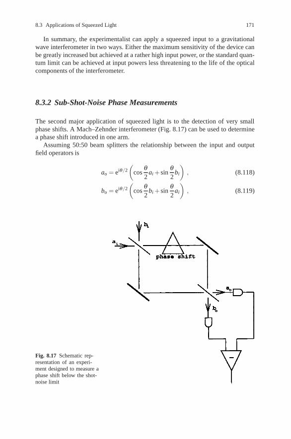
8.3 Applications of Squeezed Light 171
In summary, the experimentalist can apply a squeezed input to a gravitationalwave interferometer in two ways. Either the maximum sensitivity of the device canbe greatly increased but achieved at a rather high input power, or the standard quan-tum limit can be achieved at input powers less threatening to the life of the opticalcomponents of the interferometer.
8.3.2 Sub-Shot-Noise Phase Measurements
The second major application of squeezed light is to the detection of very smallphase shifts. A Mach–Zehnder interferometer (Fig. 8.17) can be used to determinea phase shift introduced in one arm.
Assuming 50:50 beam splitters the relationship between the input and outputfield operators is
ao = eiθ/2(
cosθ2
ai + sinθ2
bi
), (8.118)
bo = eiθ/2(
cosθ2
bi + sinθ2
ai
), (8.119)
Fig. 8.17 Schematic rep-resentation of an experi-ment designed to measure aphase shift below the shot-noise limit

172 8 Generation and Applications of Squeezed Light
where θ is the phase difference between the two arms. The two output fields aredirected onto two photo-detectors and the resulting currents combined with a 180◦power combiner. This realises a measurement of the photon number difference
c†oco = a†
oao−b†obo
= cosθ (a†i ai−b†
i bi)− i sinθ (aib†i −a†
i bi) . (8.120)
In standard interferometry the input ai is a stabilised cw laser while bi is the vacuumstate. However, as we shall show, smaller phase changes may be detected if bi isprepared in a squeezed vacuum state.
Assuming ai is in the coherent state |α〉 while bi is in the squeezed state |0, r〉,the mean and variance of the photon number difference at the output is
〈c†−c−〉= cosθ (|α|2− sinh2 r) (8.121)
V (c†−c−) = cos2 θ (|α|2 + sinh2 r cosh2r)+ sin2 θ [|α|2(1−2sinh2 r)]
− 12(α2 + α∗2)sinh2r + sinh2 r] . (8.122)
If we now set θ = π/2 + δθ , then when phase shift δθ is zero, the mean signalis zero. That is we operate on a null fringe. The Signal-to-Noise Ratio (SNR) isdefined by
SNR =〈c†−c−〉√
V (c†−c−)
. (8.123)
In the standard scheme r = 0 and
SNR = n1/2 sinδθ (8.124)
where n = |α|2. The smallest detectable phase shift is defined to be that phase forwhich SNR = 1. Thus the minimum detectable phase shift for coherent state inter-ferometry is
δθmin = n−1/2 . (8.125)
However, if bi is prepared in a squeezed vacuum state with squeezing in phase withthe amplitude α we find for moderate squeezing (|α|2� sinh2 r)
SNRss = n1/2er sinδθ (8.126)
and thus the minimum detectable phase change is
δθmin = n1/2er . (8.127)

8.3 Applications of Squeezed Light 173
The minimum detectable phase change may thus be much smaller than for co-herent state interferometry, provided we choose r < 0 i.e. phase squeezing.
Such an enhancement has been reported by Xiao et al. [22] in an experimenton the measurement of phase modulation in a Mach Zehnder interferometer. Theyreported on an increase in the signal-to-noise ratio of 3 dB relative to the shot-noiselimit when squeezed light from an optical parametric oscillator is injected into aport of the interferometer. A comparison of the fluctuations in the difference cur-rent for the cases of squeezed and a vacuum input is shown in Fig. 8.18. A similarexperiment was performed by Grangier et al. [23] employing a polarization inter-ferometer which is equivalent to a Mach–Zehnder scheme. In their experiment anenhancement factor of 2 dB was achieved.
8.3.3 Quantum Information
Squeezed states are being applied to new protocols in quantum information whichwe discuss in. In Chap. 16. Quantum information is concerned with communicationand computational tasks enabled by quantum states of light, including squeezedstates. One such application is quantum teleportation in which an unknown quantumstate is transferred from one subsystem to another using the correlations inherent ina two mode squeezed state.
Fig. 8.18 A comparison ofthe level of fluctuations inthe differenced-photocurrentfor a Mach–Zehnder inter-ferometer versus time as thephase difference is variedat a frequency of 1.6 MHz.Curve in (a) is for the caseof vacuum state input, curve(b) uses squeezed state input.The dashed line gives thevacuum level with no phasemodulation [21]

174 8 Generation and Applications of Squeezed Light
Exercises
8.1 One of the input modes of a beam splitter, with transmitivity T , is prepared ina coherent state, |α〉 and the other in a squeezed vacuum state |0,r〉. Show thatin the limit T → 1, |α| → ∞ with
√(1−T)|α| = β fixed, one of the output
states is a squeezed state with a coherent amplitude β.8.2 Calculate the squeezing spectrum for parametric oscillation in a cavity that
has different losses at each mirror for the fundamental frequency, ω1.8.3 Calculate the spectrum of fluctuations in the difference intensity, I1− I2, if an
intracavity loss is present at the idler frequency.8.4 Two photon absorption inside a cavity can be modeled by coupling the cavity
mode to a bath via the interaction Hamiltonian
H = a2Γ† +(a†)2Γ
where Γ is a reservoir operator and the reservoir is at zero temperature. Deter-mine the squeezing spectrum.
References
1. P.D. Drummond, K.J. McNeil, D.F. Walls: Optica Acta 28, 211 (1981)2. M.J. Collett, C.W. Gardiner: Phys. Rev. 30, 1386 (1984)3. M.J. Collett, D.F. Walls: Phys. Rev. A 32. 2887 (1985)4. L.A. Wu, M. Xiao, H.J. Kimble: J. Opt. Soc. Am. B 4, 1465 (1987)5. P.K. Lam, T.C. Ralph, B.C. Buchler, D. E. McClelland, H.-A. Bachor, J. Gao: J. Opt. B:
Quantum Semi-class. Opt. 1, 469 (1999)6. A.S. Lane, M.D. Reid, D.F. Walls: Phys. Rev. A 38, 788 (1988)7. S. Reynaud, C. Fabre, E. Giacobino: J. OPt. Soc Am. B 4, 1520 (1987)8. A.S. Lane, M.D. Reid, D.F. Walls: Phys. Rev. Lett. 60, 1940 (1988)9. A. Heidmann, R.J. Horowicz, S. Reynaud, E. Giacobino, C. Fabre: Phys. Rev. Lett. 59,
2555 (1987)10. Jiangrui Gao, Fuyun Cui, Chenyang Xue, Changde Xie, Peng Kunchi: Opts. Letts. 23,
870 (1998)11. O. Aytur, P. Kumar: Phys. Rev. Lett. 65, 1551 (1990)12. S.F. Pereira, M. Xiao, H.J. Kimble, J.L. Hall: Phys. Rev. A, 38, 4931 (1989)13. A. Sizman, R.J. Horowicz, G. wagner, G. Leuchs: Opt. Comms. 80, 138 (1990)14. R. Paschotta, M. Collett, P. Kurz, K. Fiedler, H.A. Bachor, J. Mlynek: Phys. Rev. Lett. 72,
3807 (1994)15. D.K. Serkland, P. Kumar, M.A. Arbore, M.M. Fejer: Opts. Letts., 22, 1497 (1997)16. C.M. Caves: Phys. Rev. Lett. 45, 75 (1980)17. W.G. Unruh: In Quantum Optics, Experimental Gravitation and Measurement Thery, ed. by
P. Meystre, M.O. Scully (Plenum, New York 1983) p.64718. R.S. Bondurant, J.H. Shapiro: Phys. Rev. D 30, 2548 (1984)19. M.T. Jaekel, S. Reynaud: Europhys. Lett. 13, 301 (1990)20. A.F. Pace, M.J. Collett, D.F. Walls: Phys. Rev. A 47, 3173 (1993)21. C.W. Misner, A.S. Thorne, J.A. Wheller: Gravitation (Freeman, San Francisco 1973)22. M. Xiao, L.A. Wu, H.J. Kimble: Phys. Rev. Lett. 59, 278 (1987)23. P. Grangier, R.E. Slusher, B. Yurke, A. La Porta: Phys. Rev. Lett. 59, 2153 (1987)

Further Reading 175
Further Reading
Bachor, H.A., J.C. Ralph: A Guide to Experiments in Quantum Optics (Wiley-VCH, 2004)Giacobino, E., C. Fabre (guest eds.): Quantum noise reduction in optical systems-experiments,
Appl. Phys. B 55(3) (1992)Kimble, H.J., D.F. Walls (guest eds.): Special Issue on Squeeze States of the Electromagnetic Field,
J. Opt. Soc. Am. B 4(10) (1987)

Chapter 9Nonlinear Quantum Dissipative Systems
Abstract In the preceding chapter we derived linearised solutions to the quantumfluctuations occurring in some nonlinear systems in optical cavities. In these solu-tions the quantum noise has been treated as a small perturbation to the solutions ofthe corresponding nonlinear classical problem. It is not possible, in general, to findexact solutions to the nonlinear quantum equations which arise in nonlinear opticalinteractions. It has, however, been possible to find solutions to some specific sys-tems. These solutions provide a test of the region of validity of the linearised solu-tions especially in the region of an instability. Furthermore they allow us to considerthe situation where the quantum noise is large and may no longer be treated as aperturbation. In this case, manifestly quantum mechanical states may be producedin a nonlinear dissipative system.
We shall give solutions to the nonlinear quantum equations for two of the prob-lems considered in Chap. 8, namely, the parametric oscillator and dispersive opticalbistability.
9.1 Optical Parametric Oscillator: Complex P Function
We shall first solve for the steady state of the parametric oscillator using the com-plex P function. Then, we show, using the positive P function, that the steady statesubharmonic field is in a superposition state. We go on to calculate the tunnellingtime between the two states in the superposition.
We consider the degenerate parametric oscillator described in Chap. 8, followingthe treatment of Drummond et al. [1]. The Hamiltonian is
H =3
∑i=0
Hi (9.1)
where
H0 = �ωa†1a1 + 2�ωa†
2a2 , (9.2)
177

178 9 Nonlinear Quantum Dissipative Systems
H1 = i�κ2
(a†21 a2−a2
1a†2) , (9.3)
H2 = i�(ε2a†2e−2iωt − ε∗2 a2e2iωt) , (9.4)
H3 = a1Γ†1 + a2Γ†
2 + h.c . (9.5)
where a1 and a2 are the boson operators for two cavity modes of frequency ω and2ω , respectively. κ is the coupling constant for the nonlinear coupling between themodes. The cavity is driven externally by a coherent driving field with frequency2ω and amplitude ε2. Γ1, Γ2 are the bath operators describing the cavity dampingof the two modes.
We recall from Chap. 8 that there are two stable steady state solutions dependingon whether the driving field amplitude is above or below the threshold amplitudeεc
2 = γ1γ2/κ . In particular, the steady states for the low frequency mode α1 are
α01 = 0, ε2 < εc
2 ,
α01 =±
[2κ
(ε2− εc2)]1/2
, ε2 ≥ εc2 . (9.6)
The master equation for the density operator of the two modes is
∂∂ t
ρ =1i�
[H0 +H1 +H2,ρ ]+ γ1(2a1ρa†1−a†
1a1ρ−ρa†1a1)
+ γ2(2a2ρa†2−a†
2a2ρ−ρa†2a2) (9.7)
where the irreversible part of the master equation follows from (6.44) for a zero-temperature bath. γ1, γ2 are the cavity damping rates.
This equation may be converted to a c-number Fokker–Planck equation using thegeneralized P representation discussed in Chap. 6. Using the operator-algebra rulesdescribed in Chap. 6, we arrive at the Fokker–Planck equation
∂∂ t
P(α) ={
∂∂α1
(γ1α1−κβ1α2)+∂
∂β1(γ1β1−κα1β2)
+∂
∂α2
(γ2α2− ε2 +
κ2
α21
)+
∂∂β2
(γ2β2− ε∗2 +
κ2
β 21
)
+12
[∂ 2
∂α21
(κα2)+∂ 2
∂β 21
(κβ2)]}
P(α) (9.8)
where (α) = [α1, β1, α2, β2].An attempt to find the steady state solution of this equation by means of a poten-
tial solution fails since the potential conditions (6.73) are not satisfied.We proceed by adiabatically eliminating the high-frequency mode. This may be
accomplished best in the Langevin equations equivalent to (9.8).

9.1 Optical Parametric Oscillator: Complex P Function 179
∂∂ t
(α1
β1
)=(
κβ1α2− γ1α1 +√
κα2[η1(t)]κα1β2− γ1β1 +
√κβ2[η1(t)]
)
∂∂ t
(α2
β2
)=(
ε2− κ2 α2
1− γ2α2
ε∗2 − κ2 β 2
2 − γ2β2
)(9.9)
where η1(t), η1(t) are delta correlated stochastic forces with zero mean
〈η1(t)〉= 〈η1(t)〉= 〈η1(t)η1(t ′)〉= 〈η1(t)η1(t ′)〉= 0 , (9.10)
〈η1(t)η1(t)〉= δ (t− t ′) . (9.11)
Under the conditions γ2� γ1 we can adiabatically eliminate α2 and β2 which givesthe resultant Langevin equation for α1 and β1
∂∂ t
(α1
β1
)=
(κγ2
(ε2− κ
2 α21
)β1− γ1α1
κγ2
(ε∗2 − κ
2 β 21
)α1− γ1β1
)+
⎛⎜⎝[
κγ2
(ε2− κ
2 α21
)]1/2η1(t)[
κγ2
(ε∗2 − κ
2 β 21
)]1/2η1(t)
⎞⎟⎠ . (9.12)
The Fokker–Planck equation corresponding to these equations is
∂∂ t
P(α1,β1) ={
∂∂α1
[γ1α1− κ
γ2
(ε2− κ
2α2
1
)β1
]
+∂
∂β1
[γ1β1− κ
γ2
(ε∗2 −
κ2
β 21
)α1
]
+12
[∂ 2
∂α21
κγ2
(ε2− κ
2α2
1
)+
∂∂β 2
1
κγ2
(ε∗2 −
κ2
β 21
)]}P(α1β1) .
(9.13)
We set ∂∂ t P(α1, β1) = 0 and attempt to find a potential solution as given by (6.72).
It is found as
F1 =−2
⎛⎝β1−
2γ2
(γ1− κ2
2γ2
)α1
2κε2−κ2α21
⎞⎠ (9.14)
F2 =−2
⎛⎝α1−
2γ2
(γ1− κ2
2γ2
)β1
2κε∗2 −κ2β 21
⎞⎠ (9.15)
It follows that the potential conditions
∂F1
∂α1=
∂F2
∂β1(9.16)
are satisfied.The potential is obtained on integrating (9.14 and 9.15)

180 9 Nonlinear Quantum Dissipative Systems
P(α) = N exp
[2α1β1 +
2γ1γ2
κ2 ln(c2−κ2α21)+ 2
(γ1γ2
κ2
)∗ln(c∗2−κ2β 2
1 )]
(9.17)where
c =√
2κε2 , γ1 = γ1− κ2
2γ2.
It is clear that this function diverges for the usual integration domain of the complexplane with β1 = α∗1. The observable moments may, however, be obtained by use ofthe complex P representation. The calculations are described in Appendix 9.A.
The semi-classical solution for the intensity exhibits a threshold behaviour atε2 = εc
2 = γ1γ2/κ . This is compared in Fig. 9.1 with the mean intensity I = 〈β1α1〉calculated from the solution (9.17), as shown in the Appendix 9.A. For comparison,the mean intensity when thermal fluctuations are dominant (Exercise 9.4) is alsoplotted. The mean intensity with thermal fluctuations displays the rounding of thetransition familiar from classical fluctuation theory. The quantum calculation showsa feature never observed in a classical system where the mean intensity actuallydrops below the semi-classical intensity. This deviation from the semi-classical be-haviour is most significant for small threshold photon numbers. As the parameterγ1γ2/κ2 is increased the quantum mean approaches the semi-classical value.
Fig. 9.1 A plot of the meanintensity for the degenerateparametric oscillator versusthe scaled driving field λ . (a)The case of zero thermal fluc-tuations. The dashed curverepresents the semi-classicalintensity, the solid curve is theexact quantum result. In bothcases μ2 = 2εc
2/κ = 5.0. Notethat above threshold the exactquantum result is less than thesemi-classical prediction. (b)The case of dominant thermalfluctuations. The mean ther-mal photon number is 10.0and μ2 = 2εc
2/κ = 100.0

9.2 Optical Parametric Oscillator: Positive P Function 181
Fig. 9.2 The log varianceof the squeezed (solid) andunsqueezed (dashed) quadra-ture in a degenerate para-metric amplifier versus thescaled driving field withμ2 = 2εc
2/κ = 5.0
The variance of fluctuations in the quadratures X1 = a1 +a†1 and X2 = (a1−a†
1)/iis given by
ΔX21 = [〈(α1 + β1)2〉− (〈α1 + β1〉)2]+ 1 , (9.18)
ΔX22 =−[〈(α1−β1)2〉− (〈α1−β1〉)2]+ 1 . (9.19)
The variance in the quadratures is plotted in Fig. 9.2a versus the scaled driving fieldλ . The variance in the phase quadrature X2 reaches a minimum at threshold. Thisminimum approaches 1
2 as the threshold intensity is increased [10]. The value of onehalf in the variance of the intracavity field corresponds to zero fluctuations foundat the resonance frequency in the external field. The fluctuations in the amplitudequadrature X1 increase dramatically as the threshold is approached. However, unlikethe calculation where the pump is treated classically the fluctuations do not diverge.This is because (9.17) is an exact solution to the nonlinear interaction includingpump depletion. As the threshold value increases and therefore the number of pumpphotons required to reach threshold increases, the fluctuations become larger. Inthe limit γ1γ2/κ2→ ∞ the fluctuations diverge, as this corresponds to the classicalpump (infinite energy). The variance in the amplitude quadrature above thresholdcontinues to increase as the distribution is then double-peaked at the two stableoutput amplitudes.
The above solution demonstrates the usefulness of the complex P representation.Although the solution obtained for the steady state distribution has no interpreta-tion in terms of a probability distribution, the moments calculated by integratingthe distribution on a suitable manifold correspond to the physical moments. Wehave demonstrated how exact moments of a quantized intracavity field undergoinga nonlinear interaction may be calculated. To calculate the moments of the externalfield however, we must resort to linearization techniques.
9.2 Optical Parametric Oscillator: Positive P Function
As an alternative to the foregoing description we may consider the use of the positiveP representation, following the treatment of Wolinsky and Carmichael [2]. We canobtain an analytic solution for the steady state positive P function. This solution is a

182 9 Nonlinear Quantum Dissipative Systems
function of two phase space variables; one variable is the classical field amplitude,the other is a non-classical variable needed to represent superpositions of coherentstates. A three-dimensional plot of the positive P function allows one to distinguishbetween the limiting regions of essentially classical behaviour and predominantlyquantum behaviour.
We begin with the Langevin equations for the low frequency mode
dαdτ
=−α−β (λ −α2)+ g(λ −α2)1/2η1 , (9.20)
dβdτ
=−β −α(λ −β 2)+ g(λ −β 2)1/2η2 , (9.21)
where τ is measured in cavity lifetimes (γ−11 ),
g =κ
(2γ1γ2)1/2≡ 1
μ, (9.22)
and λ is a dimensionless measure of the pump field amplitude scaled to give thethreshold condition λ = 1, and we have scaled the c-number variables by
α = gα1 , β = gβ1 . (9.23)
Equations (9.20 and 9.21) describe trajectories in a four-dimensional phase space.The region of phase space satisfying the conjugacy condition β = α∗ is called theclassical subspace. Two extra non-classical dimensions are required by the quantumnoise. If we neglect the fluctuating forces η1 and η2 (9.20 and 9.21) have the stablesteady state solution α = β = 0 below threshold (λ < 1), and α = β =±(λ −1)1/2
above threshold (λ > 1). In the full phase space there are additional steady stateswhich do not satisfy the conjugacy condition: two steady states α = β = ±i(1−λ )1/2 below threshold and two steady states α =−β =±(λ +1)1/2 both below andabove threshold.
The variables α and β are restricted to a bounded manifold α = x, β = y with xand y both real and |x|, |y| ≤ √λ . We denote this manifold by Λ(x, y). Trajectoriesare confined within this manifold by reflecting boundary conditions. If a trajectorystarts within this manifold, then it is clear from (9.20 and 9.21) that the drift andnoise terms remain real, so a trajectory will remain on the real plane. Furthermore,at the boundary, the trajectory must follow the deterministic flow inwards, as thetransverse noise component vanishes. If the initial quantum state is the vacuum state,the entire subsequent evolution will be confined to this manifold.
The manifold Λ(x, y) is alternatively denoted by Λ(u, υ) with u = 12 (x+y), υ =
12 (x− y). The line υ = 0 is a one-dimensional classical subspace, the subspace pre-serving α = β . The variable υ denotes a transverse, non-classical dimension usedby the noise to construct manifestly non-classical states.
We may now construct a pictorial representation of these states which dramati-cally distinguishes between the quantum and classical regimes.

9.2 Optical Parametric Oscillator: Positive P Function 183
With α = x, β = y both real, the solution to the Fokker-Planck equation (9.13) isof the form given by (9.17). With |x|, |y| ≤ √λ
Pss(x, y) = N[(λ − x2)(λ − y2)]1/g2−1e2xy/g2. (9.24)
For weak noise (g� 1), Pss(x, y) is illustrated in Fig. 9.3. Below threshold (λ < 1)Pss(u, υ) may be written
Pss(u, υ) =(1−λ 2)1/2
πλ g/2exp
(−(1−λ )u2 +(1 + λ )υ2
λ g2
2
). (9.25)
The normally-ordered field quadrature variances are determined by the quantities
〈: ΔX21 :〉= V
(α+ β
2
), (9.26)
〈: ΔX22 :〉= V
(α−β
2
)(9.27)
where V (z) refers to the variance over the stationary distribution function. As u =(α + β )/2 and υ = i(α−β )/2, on the manifold Λ(u, υ), the quadrature variancesare given by
Fig. 9.3 A plot of the positiveP representation of the steadystate of the degenerate para-metric amplifier, below andabove threshold: (a) λ = 0.8(b) λ = 1.5. In both casesg = (2εc
2/κ)−1/2 = 0.25

184 9 Nonlinear Quantum Dissipative Systems
〈: ΔX21 :〉= V (u)/g2 , (9.28)
〈: ΔX22 :〉=−V(υ)/g2 . (9.29)
The variances g−2〈Δu2〉 and −g−2〈Δυ2〉 correspond to the normally ordered vari-ances of the unsqueezed and squeezed quadratures, respectively, of the subhar-monic field.
The threshold distribution (g� 1, λ = 1) is given by
Pss(u, υ) =[
4√
πg3/2Γ(
14
)]e−(u4+4υ2)/g2
. (9.30)
Above threshold the distribution splits into two peaks. We note that in the low-noiseregime Pss(x, y) is a slightly broadened version of the classical steady state withonly a small excursion into the nonclassical space.
Figure 9.4 shows Pss(x, y) for the same values of λ as Fig. 9.3 but for thenoise strength g = 1. The quantum noise has become sufficiently strong to explore
Fig. 9.4 As in Fig. 9.3 butwith quantum noise parameterg = 1.0. (a) λ = 0.8 (b)λ = 1.5

9.2 Optical Parametric Oscillator: Positive P Function 185
thoroughly the non-classical dimension of the phase space. Pss(x, y) is strongly in-fluenced by the boundary Λ(x, y).
As the noise strength g is increased beyond 1, the characteristic threshold be-haviour of the parametric oscillator disappears and squeezing is significantly re-duced (Fig. 9.5). In the large-g limit the stochastic trajectories are all driven to theboundary of Λ(x, y), and then along this boundary to the corners, where both noiseterms in (9.20 and 9.21) vanish. Pss(x, y) approaches a sum of δ functions
Pss(x,y) =12(1 + e4λ/g2
)−1[δ (x−√
λ)δ (y−√
λ)
+ δ (x +√
λ )δ (y +√
λ )]+12(1 + e4λ/g2
)−1
× [δ (x−√
λ )δ (y +√
λ )+ δ (x +√
λ )δ (y−√
λ )] . (9.31)
The two δ functions that set x =−y = ±√λ represent off-diagonal or interferenceterms e−2
√λ/g|√λ/g〉〈−√λ/g|. Figure 9.6a–c illustrates the behaviour of Pss(x, y)
as a function of λ in the strong-noise limit. When 4λ/g2� 1 all δ functions carryequal weight and the state of the subharmonic field is the coherent state superposi-tion 1
2(|√λ/g〉+ |−√λ/g〉). As λ increases, this superposition state is replaced bya classical mixture of coherent states |√λ/g〉 and |−√λ/g〉 for 4λ/g2� 1. This isa consequence of the competition between the creation of quantum coherence by theparametric process and the destruction of this coherence by dissipation. It will beshown in Chap. 15, that the decay of quantum coherence in a damped superpositionstate proceeds at a rate proportional to the phase space separation of the states.
This example has illustrated how quantum dissipative systems can exhibit man-ifestly quantum behaviour in the limit of large quantum noise. This is outside therealm of linear noise theory where classical states are only slightly perturbed.
Fig. 9.5 As in Fig. 9.3 butwith λ = 1.5 and g = 10.0

186 9 Nonlinear Quantum Dissipative Systems
Fig. 9.6 As in Fig. 9.3 butdemonstrating the dependenceon λ with g = 5.0. (a) λ = 1.0(b) λ = 5.0 (c) λ = 10.0
9.3 Quantum Tunnelling Time
We proceed to calculate the quantum tunnelling time between the two stable states.We shall follow the procedure of Kinsler and Drummond [3]. In order to calculate

9.3 Quantum Tunnelling Time 187
the quantum tunnelling rate, we shall transform the variables α and β to give con-stant diffusion, or additive stochastic noise.
u = sin−1(
gα√λ
)+ sin−1
(gβ√
λ
), (9.32)
υ = sin−1(
gα√λ
)− sin−1
(gβ√
λ
). (9.33)
These new variables are constrained to have a range such that |u|+ |υ | ≤ π. Refer-ring back to the variables α and β , it can be seen that the u axis represents the classi-cal subspace of the phase space where α = β . Thus the variable υ is a non-classicaldimension which allows for the creation of quantum features. The stochastic equa-tions corresponding to these variables are
du ={
λ sin(u)−σ[
tan
(u + υ
2
)+ tan
(u−υ
2
)]}dτ +
√2g dWu , (9.34)
dυ ={−λ sin(υ)−σ
[tan
(u + υ
2
)− tan
(u−υ
2
)]}dτ +
√2g dWυ . (9.35)
Here σ = 1−g2/2, dWu, dWυ are Wiener processes.These Ito equations have a corresponding Fokker–Planck equation and a proba-
bility distribution in the limit as τ→ ∞ of
P(u, υ) = N exp[−V (u, υ)/g2] (9.36)
where the potential V (u, υ) is
V (u, υ) =−2σ ln |cos u + cosυ |+ λ cos u−λ cosυ . (9.37)
Above threshold the potential has two minima corresponding to the stable statesof the oscillator. These minima have equal intensities and amplitudes of oppositesign, and are at classical locations with α = α∗
(u0, υ0) = (±2sin−1[(λ −σ)1/2/√
λ ],0) (9.38)
orgα0 =±(λ −1 + g2)1/2 . (9.39)
There is also a saddle point at (us, υs) = (0, 0).Along the u axis the second derivative of the potential in the υ direction is always
positive. The classical subspace (υ = 0) is therefore at a minimum of the potentialwith respect to variations in the non-classical variable υ . This valley along the u axisbetween the two potential wells is the most probable path for a stochastic trajectoryin switching from one well to the other. The switching rate between them will bedominated by the rate due to trajectories along this route. Using an extension ofKramer’s method, developed by Landauer and Swanson [4], the mean time takenfor the oscillator to switch from one state to the other in the limit of g2� 1 is
188 9 Nonlinear Quantum Dissipative Systems
Tp =πγ1
(λ + σ
λ (λ −σ)2
)1/2
exp
{2g2
[λ −σ−σ ln
(λσ
)]}. (9.40)
The switching time is increased as the pump amplitude λ is increased or thenonlinearity g2 is reduced.
Previous attempts to compute the tunnelling time for this problem have used theWigner function [5]. Unfortunately the time-evolution equation for the Wigner func-tion contains third-order derivative terms and is thus not a Fokker–Planck equation.In the case of linear fluctuations around a steady state truncating the evolution equa-tion at second-order derivatives is often a good approximation. However, it is notclear that this procedure will give quantum tunnelling times correctly.
In the limit of large damping in the fundamental mode the truncated Wignerfunction of the sub-harmonic mode obeys with τ = γ1t
ddτ
W (β , t) ={
∂∂β
[β −β ∗(λ −g2β 2)]+∂
∂β ∗[β ∗ −β (λ −g2β ∗2)]
+∂ 2
∂β ∂β ∗(1 + 2g2β β ∗)
}W (β , τ) . (9.41)
This truncated Wigner function equation does not have potential solutions, howeveran approximate potential solution can be obtained that is valid near threshold. Here,the noise contribution 2g2β β ∗ is small and is neglected leaving only subharmonicnoise. Writing β = x + ip, the solution in the near threshold approximation is
WNT = NNT exp[−VNT(x, p)] (9.42)
where
VNT(x, p) =2g2 [g2x2 + g2p2 +
12(g2x2 + g2p2)2−λ (g2x2−g2 p2)] (9.43)
and NNT is the normalisation constant.Above threshold this potential has two minima, at gx =±(λ −1)1/2. In the limit
of large-threshold photon numbers, these minima are very close to those obtainedin (9.39). The tunneling time has been calculated from the Wigner distribution byGraham [6], with the result
Tw =πγ1
(λ + 1
λ (λ −1)2
)1/2
exp
[1g(λ −1)2
]. (9.44)
This result is compared with the expression derived using the P function in Fig. 9.7which shows the variation in the logarithm of the tunnelling rate with the pumpamplitude λ . The Wigner function result predicts a slower switching time abovethreshold. The difference in the two predictions can be many orders of magnitude.The calculations from the exact positive P Fokker–Planck equation represent a truequantum tunnelling rate. Whereas the truncation of the Wigner function equation

9.3 Quantum Tunnelling Time 189
Fig. 9.7 A plot of the log of the tunnelling time for the degenerate parametric amplifier abovethreshold, versus pump strength or noise strength. In (a) and (b) we show the results computed bythe positive P Representation (PB approximation) while in (c) and (d) we give the results for thetruncated Wigner function model. In all cases we contrast the results obtained by potential methodswith the results obtained by direct simulation of the corresponding stochastic differential equationsand number state solution of the master equation (dashed line) [3]
involves dropping higher order derivatives dependent on the interaction strength g.Thus nonlinear terms in the quantum noise are neglected and the only quantum noiseterms included are due to the vacuum fluctuations from the cavity losses. These givea diffusion term in the truncated Wigner Fokker–Planck equation which is identical

190 9 Nonlinear Quantum Dissipative Systems
to classical thermal noise, with an occupation number of half a photon per mode.Also indicated in Fig. 9.7 are the tunnelling times computed by direct numericalsimulation of the stochastic differential equations resulting from either the positiveP representation (Fig. 9.7a, b) or the Wigner representation (Fig. 9.7c, d) and bydirectly solving the master equation in the number basis.
The differences between the two rates obtained reflect the difference betweenclassical thermal activation and true quantum tunnelling. Classical thermal-activationrates are slower than quantum tunnelling rates far above threshold where the formerare large since the thermal trajectory must go over the barrier. A quantum process,on the other hand, can short cut this by tunnelling.
9.4 Dispersive Optical Bistability
We consider a single mode model for dispersive optical bistability. An optical cavityis driven off resonance with a coherent field. The intracavity medium has an inten-sity dependent refractive index. As the intensity of the driving field is increased thecavity is tuned to resonance and becomes highly transmissive.
We shall model the intracavity medium as a Kerr type χ (3) nonlinear susceptibil-ity treated in the rotating wave approximation. The Hamiltonian is given by (5.79),The Fokker–Planck equation is
∂P∂ t
=[
∂∂α
(κα+ 2iχα2β −E0)− iχ∂ 2
∂α2 α2
+∂
∂β(κ∗β −2iχβ 2α−E0)+ iχ
∂ 2
∂β 2 β 2]
P(α,β ) (9.45)
where we choose the phase of the driving field such that Eo is real and κ = γ +iδ . We shall seek a steady state solution using the potential conditions (6.72). Thecalculation of F gives
F1 =−(
iχ
)(κα
+ 2χβ − E0
α2
), F2 =
(i
χ∗
)(κ∗
α−2χ∗β − E0
β 2
), (9.46)
where we have defined κ = κ−2iχ . The cross derivatives
∂αF2 = ∂β F1 = 2 (9.47)
so that the potential conditions are satisfied.The steady state distribution is given by

9.4 Dispersive Optical Bistability 191
Pss(α, β ) = exp
⎡⎣
α∫Fρ(α′)dα′ρ
⎤⎦
= exp
⎧⎨⎩
α∫ [1iχ
(κα1
+2iχβ1−E0
α21
)dα1− 1
iχ
(κ∗β1−2iχα1−E0
β 21
)dβ1
]⎫⎬⎭
= αc−2β d−2 exp
[(E0
iχ
)(1α
+1β
)+ 4αβ
](9.48)
where c = κiχ , d =
(κiχ
)∗.
It can be seen immediately that the usual integration domain of the complex planewith α∗ = β is not possible since the potential diverges for αβ → ∞. However, themoments may be calculated using the complex P representation. The calculationsare described in Appendix 9.A. The results for the mean amplitude 〈a〉 and cor-relation function g(2)(0) are plotted in Fig. 9.8 where they are compared with thesemi-classical value for the amplitude αSS.
It is seen that, whereas the semi-classical equation predicts a bistability or hys-teresis, the exact steady state equation which includes quantum fluctuations doesnot exhibit bistability or hysteresis. The extent to which bistability is observed inpractice will depend on the fluctuations, which in turn determine the time for ran-dom switching from one branch to the other. The driving field must be ramped intime intervals shorter than this random switching time in order for bistability to beobserved.
The variance of the fluctuations as displayed by g(2)(0) show an increase as thefluctuations are enhanced near the transition point. The dip in the steady state meanat the transition point is due to out-of-phase fluctuations between the upper andlower branches.
Fig. 9.8 The steady stateamplitude, and second-ordercorrelation function for opti-cal bistability versus the pumpamplitude. The chain curvegives the semi-classical steadystate amplitude. The full curvegives the exact steady stateamplitude. The broken curvepresents the second-ordercorrelation function g(2)(0).The detuning is chosen so thatΔωχ < 0 with Λω =−10 andχ = 0.5

192 9 Nonlinear Quantum Dissipative Systems
9.5 Comment on the Use of the Q and Wigner Representations
We will compare the above solution we have obtained with the generalised P repre-sentation with the equation obtained using the Q and Wigner representations. Withthe Q representation we obtain the following equation
∂Q∂ t
(α∗,α)=[
∂∂α
(−E0 + κα+ 2iχα2α∗)+ iχ∂ 2
∂α2 α2 +(κ/2)∂ 2
∂α∂α∗+ c.c.
]Q(α∗,α)
(9.49)
where κ = κ−4iχ + iΔω .This equation has a non-positive definite diffusion matrix. Furthermore, it does
not satisfy the potential conditions, hence its steady-state solution is not readilyobtained.
The equation for the Wigner function may be shown to be as in,
∂W (α∗,α)∂ t
=(
E0∂
∂α+ κ
∂∂α
+κ2
∂ 2
∂α∗∂α−2iχ
∂∂α− iχ
12
∂ 2
∂α∗2α
+2iχ∂ 3
∂α3 α∗α2 + c.c.
)W (α∗,α) . (9.50)
This equation is not of a Fokker–Planck form since it contains third-order deriva-tives. Again a steady-state solution is not readily obtainable. It is clear that forthis problem the use of the complex P representation is preferable to the other tworepresentations.
Exercises
9.1 Derive the Fokker–Planck equation for P(α1, α2, t) for the non-degenerateparametric oscillation after adiabatically eliminating the pump mode. Solvefor the potential solution and derive the moments.
9.2 Derive the evolution equations for the Q and Wigner functions for the degen-erate parametric oscillator described by (9.1).
9.3 Derive the equation of motion for the Q function for optical bistability. Showthat with zero detuning and zero driving the solution for an initial coherentstate is
Q(α, t) =exp(−|α|2)∞
∑q, p=0
(q!p!)−1(αα∗0)q(α∗α0)p f (t)(p+q)/2
× exp
{−|α0|2 [ f (t)+ iδ ]
(1 + iδ )
}
where
δ =(p−q)/κ , f (t) = exp[−κν− iν(p−q)] , ν = 2μt , κ =γ
2μ.
9.A Appendix 193
9.4 Calculate the steady state distribution P(α) and the mean intensity 〈α∗α〉 forthe degenerate parametric oscillator for the case where the thermal fluctuationsdominate the quantum fluctuations.
9.A Appendix
9.A.1 Evaluation of Moments for the Complex P functionfor Parametric Oscillation (9.17)
It is necessary to integrate on a suitable manifold, chosen so that the distribution(9.17) and all its derivatives vanish at the boundary of integration. If we expand theterm exp(2α1 β1) in (9.17) in a power series, the expression for the moment
Inn′ =∫ ∫
β nαn′P(α)dα dβ . (9.A.1)
can be written as
Inn′ = N(2|c|)2( j2−2)∞
∑m=0
2m+2
m!
(−cκ
)m+n−1(−c∗
κ
)m+n′+1
×∫ ∫
z1j1−1(1− z1) j2− j1−1(1−2z1)m+n(1−2z2)m+n′
× z j1−12 (1− z2) j2dz1dz2 (9.A.2)
where
j1 =2γ1γ2
κ2 , j2 =4γ1γ2
κ2 , z1 =12
(1 +
κα1
c
), z2 =
12
(1 +
κβ2
c∗
).
These integrals are identical to those defining the Gauss’ hypergeometric functions.The integration path encircles each pole and traverses the Riemann sheets so thatthe initial and final values of the integrand are equal, allowing partial integrationoperations to be defined. The result is [7].
Inn′ = N′∞
∑m=0
2m
m!
(−cκ
)m+n(−c∗
κ
)m+n′
×2 F1(−(m+ n), j1, j2,2)2F1(−(m+ n), j1, j2,2) (9.A.3)
where 2F1 are hypergeometric functions.

194 9 Nonlinear Quantum Dissipative Systems
9.A.2 Evaluation of the Moments for the Complex P Functionfor Optical Bistability (9.48)
The normalization integral is
I(c, d) =∫ ∫
c
∑ 2n
n!x−c−ny−d−n exp
[E0
χ(x + y)
]dx dy (9.A.4)
where we have made the variable change x = 1/α, y = 1/β , and C is the integrationpath. α∗ = β since the potential diverges for |α|2 → ∞. This means no Glauber–Sudarshan P function exists in the steady state (except as a generalised function).Hence, we shall use the complex P function where the paths of integration for α andβ are line integrals on the individual (α, β ) complex planes.
The integrand is now in a recognisable form as corresponding to a sum of gammafunction integrals. It is therefore appropriate to define each path of integration to bea Hankel path of integration, from (−∞) on the real axis around the origin in ananticlockwise direction and back to (−∞). With this definition of the integrationdomain, the following gamma function identity holds [8]:
[Γ(c + n)]−1 =(
t1−c−n
2πi
)∫c
x−c−n exp(xt)dx . (9.A.5)
Hence, applying this result to both x and y integrations, one obtains with χ = iχ
I(c, d) =−4π2∞
∑n=0
2n(E0/χ)c+d+2(n−1)
n!Γ(c + n)Γ(d + n). (9.A.6)
The series is a transcendental function which can be written in terms of the gener-alised Gauss hypergeometric series. That is, there is a hypergeometric series called0F2 which is defined as [9]
0F2(c, d, z) =∞
∑n=0
znΓ(c)Γ(d)Γ(c + n)Γ(d + n)n!
. (9.A.7)
From now on, for simplicity, we will write just F(), instead of 0F2(). Now the nor-malisation integral can therefore be rewritten in the form
I(c, d) =(−4π2|E0/χ |c+d−2
Γ(c)Γ(d)
)F(c, d, 2|E0/χ|2) . (9.A.8)
The moments of the distribution function divided by the normalisation factor giveall the observable one-time correlation functions. Luckily the moments have ex-actly the same function form as the normalisation factor [with the replacement of(c,d) by (c+ i, d + j)] so that no new integrals need to be calculated. The ith-ordercorrelation function is

Further Reading 195
G(i) = 〈(a†)i(a)i〉=( |E0/χ|2iΓ(c)Γ(d)F(i+ c, i+ d, 2|E0/χ|2)
Γ(i+ c)Γ(i+ d)F(c, d,2|E0/χ|2))
. (9.A.9)
This is the general expression for the ith-order correlation function of a nonlineardispersive cavity with a coherent driving field and zero-temperature heat baths.
The results for the mean amplitude 〈a〉 and correlation function g2(0) are
〈a〉= 1c|E0/χ|F(1 + c, d, 2|E0/χ |2)
F(c, d, 2|E0/χ|2) , (9.A.10)
g(2)(0) =(
cdF(c, d, 2|E0/χ|2)F(c + 2, d + 2, 2|E0/χ|2)(c + 1)(d + 1)[F(c + 1, d + 1, 2|E0/χ|2)]2
). (9.A.11)
References
1. P.D. Drummond, K.J. McNeil, D.F. Walls: Optica Acta 28, 211 (1981)2. M. Wolinsky, H.J. Carmichael: Phys. Rev. Lett. 60, 1836 (1988)3. P. Kinsler, P.D. Drummond: Phys. Rev. A 43, 6194 (1991)4. R. Landauer, S. Swanson: Phys. Rev. 121, 1668 (1961)5. P.D. Drummond, D.F. Walls: J. Phys. A13 725 (1980)6. R. Graham: Quantum Statistics in Optics and Solid State Physics, Springer Tracts Mod. Phy.,
Vol. 66 (Springer, Berlin, Heidelberg 1973)7. T.M. MacRobert: Function of a Complex Variable (Macmillan, London 1938)8. M. Abramowitz, I.A. Stegun: Handbook of Mathematical Function (Dover, New York 1965)9. I.S. Gradsteyn, I.M. Ryzhik: Tables of Series, Products and Integrals, (Deutsch, Frank-
furt/M 1981)10. G.J. Milburn, D.F. Walls: Optics Commun. 39, 401 (1981)
Further Reading
Gibbs, H.: Optical Bistability, Academic Press (1985)Lugiato, L.A. in Progress in Optics, p. 69, Ed. E. Wolf, North-Holland (1984)

Chapter 10Interaction of Radiation with Atoms
Abstract The preceding chapters have been concerned with the properties of theradiation field alone. In this chapter we turn to the interaction between radiationand matter. This is of course the domain of quantum electrodynamics, however inquantum optics we are usually only concerned with low energy systems of boundelectrons which simplifies matters considerably. We will use the occupation num-ber representation for bound many-electron systems to quantize the electronic de-grees of freedom, following the approach of Haken [1] and also Cohen-Tannoudjiet al. [2].
10.1 Quantization of the Many-Electron System
In the full theory of QED, the interaction between the electromagnetic field andcharged matter is described by coupling between the vector potential and the Diracspinor field. In quantum optics we only need the low energy (non relativistic) limitof this interaction. This is given by the minimal coupling Hamiltonian [3]
H =1
2m(�p− e�A)2 + eV(�x)+ Hrad (10.1)
where �p is the momentum operator for a particle of charge e moving in a Coulombpotential V (�x). The vector potential is quantised in a box of volume V as
�A(�x,t) = ∑n,ν
√h
2εoωnV�en,ν
[ei(�kn.�x−ωnt)an,ν + e−i(�kn.�x−ωnt)a†
n,ν
](10.2)
where �en,ν are two orthonormal polarisation vectors (ν = 1,2) which satisfy �kn ·�en,ν = 0, as required for a transverse field, and the frequency is given by the dis-persion relation ωn = c|�kn|. The positive and negative frequency Fourier operators,respectively an,ν and a†
m,ν , satisfy
197

198 10 Interaction of Radiation with Atoms
[an,ν ,an′,ν ′ ] = δνν ′δnn′ (10.3)
The last term, Hrad is the Hamiltonian of the free radiation field given by
Hrad = ∑k
hωka†kak (10.4)
where we have subsumed polarisation and wave vectors labels into the single sub-script k.
We now use an occupation number representation in the antisymmetric sectorof the many body Hilbert space for the electronic system based on a set of singleparticle states |φ j〉, with position probability amplitudes, φ j(�x), which we take as thebound energy eigenstates of the electronic system without radiation. They could forexample be the stationary states of a atom, the quasi bound states of a single Cooperpair on a mesoscopic super-conducting metal island, or the bound exciton states ofsemiconductor quantum dot. We then define the electronic field operators
ψ(�x) = ∑j
c jφ j(�x) (10.5)
where the appropriate commutations relations for the antisymmetric sector are thefermionic forms
ckc†l + clc
†k = δkl (10.6)
ckcl + clck = c†kc†
l + c†l c†
k = 0 (10.7)
In the occupation number representation the Hamiltonian may be written as thesum of three terms, H = Hel + HI + Hrad where the electronic part is given by
Hel =∫
d3�xψ†(�x)[− h2
2m∇2 + eV(�x)
]ψ(�x) = ∑
j
E jc†j c j (10.8)
The interaction part may be written as the sum of two terms HI = HI, 1 +HI, 2 where
Hl, 1 =∫
d3�xψ†(�x)(− e
2m(�A(�x).�p+�p.�A(�x))
)ψ(�x) (10.9)
Hl, 2 =∫
d3�xψ†(�x)(
e2
2m(�A(�x)2
)ψ(�x) (10.10)
Unless we are dealing with very intense fields for which multi-photon processes areimportant, the second term HI, 2 may be neglected.
The dominant interaction energy may then be written as
HI = h ∑�k,n,m
g�k,n,m(b�k + b†�k)c†
ncm (10.11)
where the interaction coupling constant is

10.1 Quantization of the Many-Electron System 199
g�k,n,m =− em
(1
2ε0hωkV
)1/2∫d3�xφ∗n(�x)
(ei�k.�x�p
)φm(�x) (10.12)
We now proceed by making the dipole approximation. The factor ei�k�x varies on aspatial scale determined by the dominant wavelength scale, λ0, of the field state. Atoptical frequencies, λ0 ≈ 10−6 m. However the atomic wave functions, φn(�x) varyon a scale determined by the Bohr radius, a0 ≈ 10−11 m. Thus we may remove theoscillatory exponential from the integral and evaluate it at the position of the atom�x =�x0. Using the result
[�p2, �x] =−i2h�p (10.13)
we can write the interaction in terms of the atomic dipole moments∫
d3�xφ∗n(�x)(
ei�k.�x�p)
φm(�x) = ime
ωnmei�k.�x0
∫d3�xφ∗n(�x)(e�k)φm(�x) (10.14)
where ωnm = (En−Em)/h.In the interaction picture the interaction Hamiltonian becomes explicitly time
dependent,
HI(t) = h ∑�k,n,m
g�k,n,m(b�ke−iω(�k)t + b†�k
eiω(�k)t)c†ncmeiωnmt (10.15)
where the tilde indicates that we are in the interaction picture. If the field is in statefor which the dominant frequency is such that ω(�k0) ≈ ωnm, the field is resonantwith a particular atomic transition and we may neglect terms rotating at the veryhigh frequency ω(�k)+ωnm. This is known as the rotating wave approximation. Thisassumes that the field strength is not too large and further that the state of the fielddoes not vary rapidly on a time scale of ω−1
nm i.e. we ignore fields of very fast strongpulses. As a special case we assume the field is resonant (or near-resonant) with asingle pair of levels with E2 > E1. The interaction picture Hamiltonian in the dipoleand rotating wave approximation is then given by
HI = h∑�k
c†1c2b†
�kg�ke−i(ω(�k)−ω21)t + h.c (10.16)
where
g�k =−i(
2hε0ω(�k)V)−1/2
ωaμ21ei�k.�x0 (10.17)
andμ21 = 〈φn|e�x|φm〉 (10.18)
with ωa = ω2−ω1.It is conventional to describe the operator algebra of a two level system in terms
of pseudo-spin representation by noting that the Pauli operators may be defined as

200 10 Interaction of Radiation with Atoms
σz = c†2c2− c†
1c1 (10.19)
σx = c†2c1 + c†
1c2 (10.20)
σy =−i(c†2c1− c†
1c2) (10.21)
σ+ = σ†− = c†
2c1 (10.22)
The operators sα = σα/2 (with α = x,y,z) then obey the su(2) algebra for a spinhalf system. In terms of these operators we may write the total Hamiltonian for thesystem of field plus atom in the dipole and rotating wave approximation as
H = ∑�k
hω(�k)b†�k
b�k +hωa
2σz + h∑
�k
g�kb�kσ+ + h.c . (10.23)
The free Hamiltonian for the two-level electronic system is
Hel =hωa
2σz (10.24)
Denoting the ground and excited states as |1〉 and |2〉 respectively, we see that
Hel|s〉= (−1)s hωa
2|s〉 s = 1,2 (10.25)
The action of the raising and lowering operators on the energy eigenstates is:σ+|1〉 = |2〉 and σ−|2〉 = |1〉, while σ2± = 0. We now relabel the ground state andexcited state respectively as |1〉 ≡ |g〉, |2〉 ≡ |e〉. If the state of the system at time t isρ , the probability to find the electronic system in the excited state and ground stateare, respectively,
pe(t) = 〈2|ρ|2〉= 〈σ+σ−〉 (10.26)
pg(t) = 〈1|ρ|1〉= 〈σ−σ+〉 (10.27)
The atomic inversion is defined as the difference between these two probabilitiesand is given by
pe(t)− pg(t) = 〈σz〉 (10.28)
While the atomic coherences are defined by
ρ12 ≡ 〈1|ρ|2〉= 〈σ+〉 (10.29)
with ρ21 = ρ∗12.

10.2 Interaction of a Single Two-Level Atom with a Single Mode Field 201
10.2 Interaction of a Single Two-Level Atomwith a Single Mode Field
If we further restrict the state of the field to include only a single mode, withfrequency ω0; perhaps using a high Q optical resonator, we arrive at the Jaynes–Cummings hamiltonian,
H = hω0b†b +hωa
2σz + h(gbσ+ + g∗b†σ−) (10.30)
coupling a single harmonic oscillator degree of freedom to a two-level system,which might well be called the standard model of quantum optics [4]. The couplingconstant g can vary from a few kHz to many MHz. An example is provided by theexperiment of Aoki et al. [5] in which a cesium atom interacts with the toroidal whis-pering gallery mode of a micro-resonator as it falls under the action of gravity froma magneto-optical trap. The atomic resonance at is the 6S1/2; F = 4→ 6P3/2; F ′= 5transition in cesium. A coupling constant as large as g/2π = 50MHz was achieved.
On resonance, ωa = ωc = ω, we see that the interaction Hamiltonian HI =hg(bσ+ + b†σ−) (with g chosen as real), commutes with the free Hamiltonian,H0 = hω(b†b + 1
2 σz), so that the eigenstates of the full Hamiltonian can be writ-ten as a linear combination of the degenerate eigenstates of H0. Defining |n,s〉 =|n〉b⊗ |s〉, where b†b|n〉= n|n〉, the degenerate eigenstates of the free Hamiltonianare |n,2〉, |n+1,1〉. Within this degenerate subspace, the state at time t may be writ-ten |ψn(t)〉= cn,2(t)|n,2〉+cn+1,2(t)|n+1,1〉, and the Schroedinger equation in theinteraction picture is
(cn,2
cn+1,1
)=−iΩnσx
(cn,2
cn+1,1
)(10.31)
where Ωn = g√
n + 1. The eigenvalues of this system of linear equations are ±iΩn,corresponding to the eigenstates of HI
|n,±〉= 1√2(|n,2〉± |n + 1,1〉) (10.32)
which are often referred to as the dressed states. The splitting of the degeneracy isdepicted in Fig. 10.1.
Thus the general solution is
cn,2(t) = cn,2(0)cosΩnt− icn+1,1(0)sin Ωnt (10.33)
cn+1,1(t) = cn+1,1(0)cosΩnt− icn,2(0)sin Ωnt (10.34)
If the atom is initially in the excited state and the cavity field has exactly n photons,the probability for finding the atom in the same state at time t > 0 is
pe(t) = |〈n,2|ψn(t)〉|2 =12(1 + cos2Ωnt) (10.35)

202 10 Interaction of Radiation with Atoms
(|1>|g >, |0>|e >)
.
.
.
.(|2 >|g >, |1>|e >)
(|n + 1>|g >,|n >|e >)
|1,–>
|1,+>
|2, –>
|2, +>
|n, –>
|n, +>
2g
2g
2 2 g
n + 1
Fig. 10.1 The dressed states for the energy eigenstates of the Jaynes–Cummings interaction. Onthe left are show the degenerate states for zero interaction. When the interaction is turned on thedegeneracies are lifted
The excitation oscillates backward and forth between the cavity and the electronicsystem with frequency Ωn, the Rabi frequency. Note that for n = 0 the separation ofthese eigenvalues is 2g, which is known as the vacuum Rabi splitting.
If the field is in an arbitrary pure state, |φ〉 = Σn fn|n〉 and the atom is initiallyexcited, the probability to find the atom in the excited state at time t > 0 may bewritten
pe(t) =12
[1 +
∞
∑n=0| fn|2 cos(2g
√n + 1t)
](10.36)
This is a discrete superposition of harmonic oscillations with incommensurate fre-quencies. Thus it must exhibit quasiperiodic behaviour. If the initial photon numberdistribution | fn|2 has narrow support on n, only a few frequencies are involved andthere is a beating between these different frequencies leading to what are knownas collapses and revivals. The collapse refers to the decay of oscillations at shorttimes due to beating between the incommensurate frequencies. The revival refers topartial re-phasing of the oscillations at later times. In the case of the field initiallyin a coherent state, |α〉, the initial number distribution is Poissonian with standarddeviation in number given by the root mean, n1/2|α|. An approximate evaluation ofthe sum valid for times such that gt < n1/2 gives [6]
pe(t) =12
[1 + e
− g2t2 n2(n+1) cos(2g
√n+ 1t)
](10.37)
There is an average Rabi oscillation frequency under a Gaussian envelope. The char-acteristic time for the collapse of the oscillation is thus

10.3 Spontaneous Emission from a Two-Level Atom 203
Fig. 10.2 (a) The experimen-tal observation of collapse andrevival of the oscillations inthe occupation of the excitedstate of a two-level atom inter-acting with a microwave fieldinitially in a coherent statewith mean photon numbern = 0.85. In (b) is the Fouriertransform of the oscillationswith the Rabi frequenciesΩn, n = 0, 1, 2, 3 marked(from [7])
tcol ∼ 1g
(10.38)
A more accurate evaluation using the Laplace summation formulae shows that theoscillations first revive at a t time
trev ∼ 2πg
n1/2 (10.39)
Thus a quasi periodic burst of Rabi oscillations occurs every n Rabi periods. Thecollapse and revival has been seen experimentally using an atom excited to a Rybergground state interacting with the microwave field in a superconducting cavity [7].The results of the experiment are shown in Fig. 10.2.
10.3 Spontaneous Emission from a Two-Level Atom
Spontaneous emission can also be treated using a master equation. In this case thesystem is a two-level electronic system, with ground state |g〉 of energy hω1 and ex-cited state |e〉 with energy hω2, representing an electric dipole transition, coupled tothe many modes of the radiation field in the dipole and rotating wave approximation.The master equation is

204 10 Interaction of Radiation with Atoms
dρdt
=− i
h[H,ρ]+ γ(n+ 1)D [σ−]ρ + γ nD [σ+]ρ (10.40)
where n is the thermal occupation of the radiation field mode at the atomic resonancefrequency ωa = ω2−ω1. We have neglected a small term which gives rise to ashift in the atomic transition frequency and which contributes to the Lamb shift.At optical frequencies, n ≈ 0. In the case of a free two-level atom, H = hωa
2 σz theprobability to find the atom in the excited state, pe(t) = 〈e|ρ|e〉 satisfies the equation
dpe
dt=−γ pe(t) (10.41)
with the solution pe(t) = pe(0)e−γt , which describes spontaneous emission. Thedipole polarisation is proportional to the atomic coherence, 〈e|ρ|g〉 = 〈σ−〉 whichobeys
d〈σ−〉dt
=−(
iωa +γ2
)〈σ−〉 (10.42)
with the solution〈σ−(t)〉= 〈σ−(0)〉e−(γ/2+iωa)t (10.43)
The dipole oscillates at the transition frequency and decays, as it radiates.The radiated field is related to the input field and the local source through an in-
put/output relation in analogy with the case of a cavity discussed above. The positivefrequency components of the field operator takes the form
E(+o (�x,t) = E(+)
i (�x,t)− ω2a
4πε0c2r
(�μ×�x
r
)�x
rσ−(t− x/c) (10.44)
where r = |�x| is the distance from the source to the point�x and�μ is the atomic dipolemoment.
10.4 Phase Decay in a Two-Level System
Spontaneous emission is not the only irreversible process involved in the absorptionand emission of light. In an atomic vapour, atomic collisions are also a source of de-coherence and cause a decay of the atomic polarisation, σx + iσy, without changingthe decay of the inversion, σz. We can model this process by a coupling between theinversion and a high temperature heat bath,
Hcol = σzΓc(t) (10.45)
where Γc(t) is a bath operator describing the collisions. This Hamiltonian com-mutes with σz and thus does not contribute to the decay of the inversion. It appearslike a fluctuating detuning in the Bloch equations and thus will effect the atomic
10.5 Resonance Fluorescence 205
polarisation. The corresponding master equation, in the interaction picture and in-cluding spontaneous emission, is
dρdt
=γ2(2σ−ρσ+−σ+σ+ρ−ρσ+σ+)− γp[σz, [σz[,ρ]] (10.46)
The Bloch equations now become
d〈σz〉dt
=−γ(〈σz〉+ 1) (10.47)
d〈σx〉dt
=−( γ
2+ γp
)〈σx〉 (10.48)
d〈σy〉dt
=−( γ
2+ γp
)〈σy〉 (10.49)
In the presence of collisions the decay time for the polarisation, T2, is no longergiven by twice the decay time for the inversion, T1 = γ−1, but rather T2 < 2T1.
10.5 Resonance Fluorescence
If the atom is driven by a classical radiation field, the Hamiltonian becomes (see(10.30) and replace b �→ β)
H =hωa
2σz + Ω(σ+e−iωLt + σ−eiωLt) (10.50)
where Ω = gβ is the Rabi frequency and ωL is the carrier frequency of the drivingfield. The master equation in an interaction picture at the frequency ωL is
dρdt
=−iΔω2
[σz,ρ]− iΩ[σ+ + σ−,ρ]+ γD [σ−]ρ (10.51)
where the detuning is Δω = ωa−ωL. The resulting Bloch equations for the atomicmoments are linear
d〈σ−〉dt
=−(γ
2+ iΔω
)〈σ−〉+ iΩ〈σz〉 (10.52)
d〈σz〉dt
=−γ(〈σz〉+ 1)−2iΩ(〈σ+〉− 〈σ−〉) (10.53)
These inhomogeneous equations can be written as homogeneous equations as
ddt
(〈�σ(t)〉− 〈�σ〉ss) = A(〈�σ(t)〉− 〈�σ〉ss) (10.54)

206 10 Interaction of Radiation with Atoms
where
A =
⎛⎝−
( γ2 − iΔω
)0 −iΩ
0 −( γ2 + iΔω
)iΩ
−2iΩ 2iΩ −γ
⎞⎠ (10.55)
with 〈�σ〉= (〈σ+〉,〈σ−〉,〈σz〉)T and the steady state solutions are
〈σz〉ss =− 1 + δ2
1 + δ2 + Z2(10.56)
〈σ+〉ss =i√2
Z(1 + iδ)1 + δ2 + Z2
(10.57)
with
Z =2√
2Ωγ
, δ =2Δω
γ(10.58)
The solutions for resonance (Δω = 0), with the atom initially in the ground state,are
〈σz(t)〉= 8Ω2
γ2 + 8Ω2
[1− e−3γt/4
(cosh κt +
3γ4κ
sinh κt
)]−1 (10.59)
〈σ+(t)〉= 2iΩγ
γ2 + 8Ω2
[1− e−3γt/4
(cosh κt +
(κγ
+3γ
16κ
)sinh κt
)](10.60)
where
κ =12
√γ2
4−16Ω2 (10.61)
Clearly there is a threshold at Ω = γ/8 below which the solutions monotonicallyapproach the steady state and above which they are oscillating. A similar thresholdoccurs in the solutions for the two-time correlation function 〈σ+(t)σ−(t + τ)〉t→∞which determines the spectrum of the scattered light.
The stationary spectrum, as measured by a monochromatic detector at the point�x is defined by [9]
S(�x,ω) = limt→∞
12π
∫ ∞
−∞〈E(−)(�x,t)E(+)(�x,t + τ)〉dτ (10.62)
the Fourier transform of the stationary two-time correlation function〈E(−)(t)E(+)(t + τ)〉 which using (10.44) is given by
S(�x,ω) =I0(�x)2π
∫ ∞
−∞dτe−iωτG(τ) (10.63)

10.5 Resonance Fluorescence 207
where
I0(�x) =∣∣∣∣ ω2
0
4πε0c2r
(�μ×�x
r
)�x
r
∣∣∣∣2
(10.64)
andG(τ) = lim
t→∞〈σ+(t)σ−(t + τ)〉 ≡ 〈σ+σ−(τ)〉ss (10.65)
with〈σ+(t)σ−(t + τ)〉= tr
[σ−eL τρ(t)σ+
](10.66)
The equation of motion for G(τ) couples in many other moments. If we define thecorrelation matrix
G (τ) =
⎛⎝〈σ+σ+(τ)〉ss 〈σ−σ+(τ)〉ss 〈σzσ+(τ)〉ss
〈σ+σ−(τ)〉ss 〈σ−σ−(τ)〉ss 〈σzσ−(τ)〉ss
〈σ+σz(τ)〉ss 〈σ−σz(τ)〉ss 〈σzσz(τ)〉ss
⎞⎠ (10.67)
The quantum regression theorem indicates that G (τ) as a function of τ obeys thesame equations of motion as 〈�σ(τ)〉− 〈�σ〉ss,
G (τ)dτ
= AG (τ) (10.68)
The initial conditions are simplified due to the algebra of the Pauli matrices, forexample σ+σ− = (σz + 1)/2 and σ2± = 0, and may thus be written in terms of thestationary solutions in (10.57). On resonance we find that in the Schrodinger picture,
G(τ) =4Ω2
γ2 + 8Ω2
[γ2
γ2 + 8Ω2 e−iωat +12
e−(γ/2+iωa)τ
− 12
(γ2
γ2 + 8Ω2
3γ/4 + κκ
− γ/2κ− γ/4 + κ
2κ
)exp{−(3γ/4−κ+ iωa)τ}
+12
(γ2
γ2 + 8Ω2
3γ/4−κκ
− γ/2κ− γ/4−κ
2κ
)exp{−(3γ/4 + κ+ iωa)τ}
]
(10.69)
with τ ≥ 0. The corresponding spectrum has a single Lorentzian peak for weakdriving fields, 4Ω << γ2/16,
S(�x,ω) = I0(r)4Ω2
γ2 + 8Ω2 δ(ω−ωa) (10.70)
which corresponds to elastic scattering. For very strong driving fields, Ω >> γ wefind that the spectrum acquires three Lorentzian peaks at ω = ωa and ω = ωa±2Ω.The spectrum, including the elastic term, is

208 10 Interaction of Radiation with Atoms
S(�x,ω) =I0(r)2π
(2π
4Ω2
γ2 + 8Ω2 δ(ω−ωa)+12
γ/2γ2/4 +(ω−ωa)2
+14
3γ/4(3γ/4)2 +[ω− (ω+ 2Ω)]2
+14
3γ/4(3γ/4)2 +[ω− (ω−2Ω)]2
)
(10.71)
This is the Mollow spectrum [10].The light scattered by a two-level atom also exhibits photon anti-bunching. Con-
sider the conditional probability that given a photon is counted at time t anotherphoton will be counted a time τ later. This is proportional to the second order corre-lation function
G(2)(t,τ) = 〈a†(t)a†(t + τ)a(t + τ)a(t)〉 (10.72)
Usually we are interested in a stationary source so we let t → ∞ and we normalisethis by the intensity squared to define
g(2)(τ) = limt→∞
G(2)(t,τ)〈a†(t)a(t)〉2 (10.73)
Using the result in (10.44) we can express this directly in terms of correlation func-tions for the atomic polarisation. As the equations of motion for the atomic variablesare linear, the stationary correlation function 〈σ+(t)σ+(t +τ)σ−(t +τ)σ−(t)〉t←∞ isgiven by the quantum regression theorem. We then find that
g(2)(τ) = 1− e−3γt/4(
cosh κτ+3γ4κ
sinh κτ)
(10.74)
The result g(2)(τ = 0)= 0 indicates photon anti-bunching, as the probability to counta second photon, immediately after a first one has been counted, vanishes. This isa direct result of the emission process of the source. Photons are emitted when anexcited atom relaxes back to the ground state. If a photon is counted, the atom islikely to be in ground state and thus a finite time must elapse before it is re-excitedand capable of emitting another one. The probability to find the atom in the excitedstate at time τ given that it starts in the ground state at τ = 0 is
Pe(τ) =4Ω2
γ2 + 8Ω2
[1− e−3γτ/4
(cosh κτ+
3γ4κ
sinh κτ)]
(10.75)
Comparison with (10.74) indicates this interpretation is correct. This prediction,first made by Carmichael and Walls [8], was one of the earliest examples of howquantum optics would differ from a semiclassical description of light. In Fig. 10.3we plot g(2)(τ) for two values of the Rabi frequency.
The first observation of photon antibunching was made by Kimble et al. in 1977on atomic beams [11]. They saw a positive slope for g(2)(τ) which is consistentwith the predictions of the theory, however fluctuations from atomic numbers in thebeam made a detailed comparison with the single atom result impossible. Ion traps
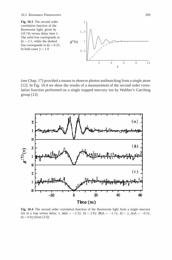
10.5 Resonance Fluorescence 209
Fig. 10.3 The second ordercorrelation function of thefluorescent light, given by(10.74) versus delay time τ.The solid line corresponds toΩ = 2.5, while the dashedline corresponds to Ω = 0.25.In both cases γ = 1.0
2 4 6 8 10
0.5
1
1.5
2
g(2)(τ)
τ
(see Chap. 17) provided a means to observe photon antibunching from a single atom[12]. In Fig. 10.4 we show the results of a measurement of the second order corre-lation function performed on a single trapped mercury ion by Walther’s Garchinggroup [13].
Fig. 10.4 The second order correlation function of the fluorescent light form a single mercuryion in a trap versus delay, τ. (a)Δ = −2.3γ , Ω = 2.8γ . (b)Δ = −1.1γ , Ω = γ , (c)Δ = −0.5γ ,Ω = 0.6γ (from [13])

210 10 Interaction of Radiation with Atoms
Exercises
10.1 In the Jaynes–Cummings model, show that if the atom begins in the groundstate and the field begins in the state |φ〉= Σ fn|n〉, the probability to find theatom in the excited state at time t > 0 is given by
pe(t) =∞
∑n=1
| fn|2 sin2(Ωn−1t) (10.76)
10.2 In the Jaynes–Cummings model, show that if the atom begins in the groundstate and the field begins in the state |φ〉 = Σ fn|n〉, the state at time t > 0 isthe entangled state
|ψ(t)〉= |φg(t)〉|g〉+ |φe(t)〉|e〉 (10.77)
where
|φg(t)〉= ∑n
fn cos(Ωn−1t) (10.78)
|φe(t)〉= i∑n
fn sin(Ωn−1t) (10.79)
In the case of the field initially in a coherent state, plot the Q-functions for|φe(t)〉 and |φe(t)〉 at times equal to half way to the first revival and at the firstrevival.
10.3 Compute the dressed states, and the corresponding eigenvalues, for the case inwhich the field mode is detuned from the atomic resonance, Δ = ωa−ωc �= 0.
10.4 Define the trace-preserving density operator map on the state of a single two-level system,
ρ �→ E (ρ) = σzρσz (10.80)
Sow that this leaves unchanged the diagonal elements of ρ in the eigenstatesof σz, but changes the phase of the off-diagonal elements by π.
10.5 Calculate the second order correlation function g(2)(τ) for resonance fluores-cence in the presence of atomic dephasing (see (10.46).
References
1. H. Haken: Waves, Photons and Atoms (North Holland, Amsterdam, 1981) Vols. 1 and 2.2. C. Cohen-Tannoudji, J. Dupont-Roc, G. Grynberg: Photons and Atom-Introduction to Quan-
tum Electrodynamics (Wiley-Interscience, 1997).3. R. Loudon: Quantum Theory of Light (Oxford University Press, Oxford 1973).4. B.W. Shore, P.L. Knight: The Jaynes–Cummings Model, J. Mod. Opt. 40, 1195–1238 (1993).5. T. Aoki, B. Dayan, E. Wilcut, W.P. Bowen, A.S. Parkins, T.J. Kippenberg, K.J. Vahala, H.J.
Kimble: Observation of Strong Coupling Between One Atom and a Monolithic Microres-onator, Nature 443, 671 (2006).

Further Reading 211
6. S. Haroche: In New Trends in Atomic Physics, ed. by G. Grynberg, R. Stora, Les HoucheSession XXXVIII (Elsevier, Amsterdam 1984).
7. J.M. Raimond, M. Brune, S. Haroche: Rev. Mod. Phys. 73, 565–582 (2001).8. H.J. Carmichael, D.F. Walls: Proposal for the Measurement of the Resonant Stark Effect by
Photon Correlation Techniques, J. Phys. B 9, L43 (1976).9. R.J. Glauber: Phys. Rev. 131, 2766 (1963).
10. B.R. Mollow: Phys. Rev. 188, 1969 (1969).11. H.J. Kimble, M. Degenais, L. Mandel: Phys. Rev. Lett. 39, 691 (1977).12. F. Diedrich, H. Walther: Phys. Rev. Lett. 58, 203 (1987).13. H. Walther: Proc. R. Soc. Lond. A 454, 431 (1998).
Further Reading
Allen, L., J. Eberly: Optical Resonance and Two-Level Atoms (Wiley, New York 1975)Cohen-Tannoudji, C., J. Duppont, G. Grynberg: Photons and Atoms: Introduction to Quantum
Electrodynamics (Wiley, New York 1989)Mollow, B.R.: Progress in Optics 19 (North-Holland, Amsterdam 1987). H.J. (Springer, Berlin
1999)Carmichael, H.J. “Statistical methods in quantum optics 1: Master equations and Fokker-Planck
equations” (Springer, Berlin, 1999)

Chapter 11CQED
Abstract In this chapter we will discuss two different physical systems in which asingle mode of the electromagnetic field in a cavity interacts with a two-level dipoleemitter. In the first example, the system is comprised of a single two-level atominside an optical cavity. The study of this system is often known as cavity quantumelectrodynamics (cavity QED) as it may be described using the techniques of theprevious chapter.
The second example is comprised of a superconducting Cooper pair box insidea co-planar microwave resonator. The description of this system is given in termsof the quantisation of an equivalent electronic circuit and thus goes by the name ofcircuit quantum electrodynamics (circuit QED).
In both cases we are typically interested in the strong coupling regime in whichthe single photon Rabi frequency g (the coupling constant in the Jaynes–Cummingsmodel) is lager than both the spontaneous decay rate, γ , of the two-level emitter andthe rate, κ , at which photons are lost from the cavity.
11.1 Cavity QED
The primary difficulty we face in cavity QED is finding a way to localise a singletwo-level atom in the cavity mode for long time intervals. One approach, pioneeredby the Caltech group of Kimble [1], is to first trap and cool two-level atoms in amagneto-optical trap (MOT) (see Chap. 18) and then let them fall into a high finessecavity placed directly below the MOT. If the geometry is correctly arranged then atmost one atom will slowly fall through the cavity at a time. Another approach is touse constraining forces to trap a single atom in the optical cavity. This can be doneusing the light shift forces of a far off resonant laser field on a two-level atom[2, 3](see Chap. 18), or it can be done using an ion trap scheme [4] (see Chap. 17). Avery novel way to get atoms from the MOT into the cavity deterministically hasbeen pioneered by the Chapman group in Georgia [5]. They use an optical dipolestanding wave trap as a kind of atomic conveyor belt to move atoms from the MOTinto the cavity.
213
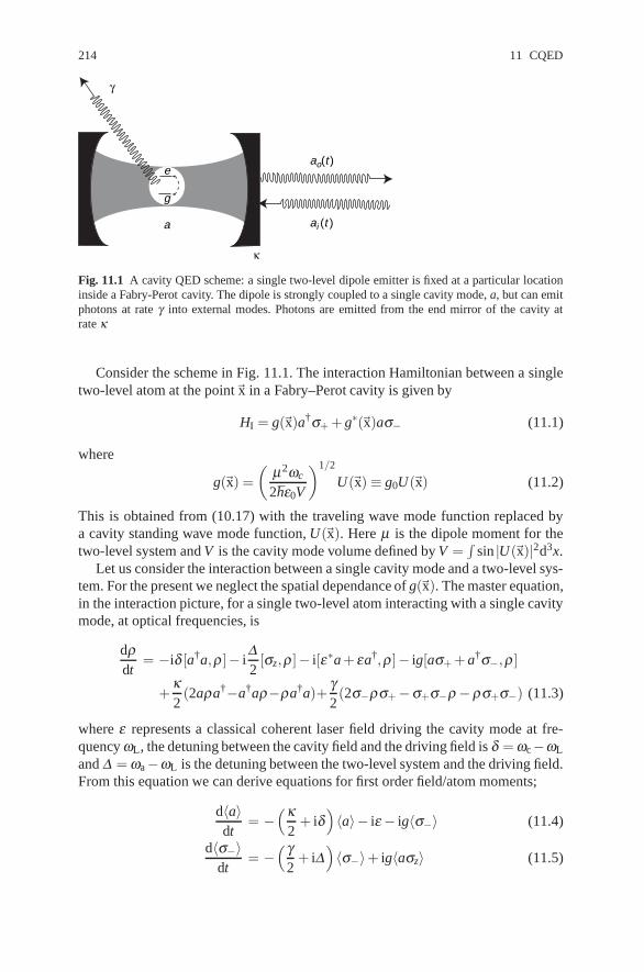
214 11 CQED
ai (t )
ao(t )
κ
a
γ
g
e
Fig. 11.1 A cavity QED scheme: a single two-level dipole emitter is fixed at a particular locationinside a Fabry-Perot cavity. The dipole is strongly coupled to a single cavity mode, a, but can emitphotons at rate γ into external modes. Photons are emitted from the end mirror of the cavity atrate κ
Consider the scheme in Fig. 11.1. The interaction Hamiltonian between a singletwo-level atom at the point�x in a Fabry–Perot cavity is given by
HI = g(�x)a†σ+ + g∗(�x)aσ− (11.1)
where
g(�x) =(
μ2ωc
2hε0V
)1/2
U(�x)≡ g0U(�x) (11.2)
This is obtained from (10.17) with the traveling wave mode function replaced bya cavity standing wave mode function, U(�x). Here μ is the dipole moment for thetwo-level system and V is the cavity mode volume defined by V =
∫sin |U(�x)|2d3x.
Let us consider the interaction between a single cavity mode and a two-level sys-tem. For the present we neglect the spatial dependance of g(�x). The master equation,in the interaction picture, for a single two-level atom interacting with a single cavitymode, at optical frequencies, is
dρdt
= −iδ [a†a,ρ ]− iΔ2
[σz,ρ ]− i[ε∗a + εa†,ρ ]− ig[aσ+ + a†σ−,ρ ]
+κ2
(2aρa†−a†aρ−ρa†a)+γ2(2σ−ρσ+−σ+σ−ρ−ρσ+σ−) (11.3)
where ε represents a classical coherent laser field driving the cavity mode at fre-quency ωL, the detuning between the cavity field and the driving field is δ = ωc−ωL
and Δ = ωa−ωL is the detuning between the two-level system and the driving field.From this equation we can derive equations for first order field/atom moments;
d〈a〉dt
= −(κ
2+ iδ
)〈a〉− iε− ig〈σ−〉 (11.4)
d〈σ−〉dt
= −(γ
2+ iΔ
)〈σ−〉+ ig〈aσz〉 (11.5)

11.1 Cavity QED 215
d〈σz〉dt
= −γ(〈σz〉+ 1)−2ig(〈aσ+〉− 〈a†σ−〉) (11.6)
Looking at these equations we see that we do not get a closed set of equations forthe first order moments, for example the equation for 〈σ−〉 is coupled to 〈aσz〉. Anumber of procedures have been developed to deal with this. If there are many atomsinteracting with a single mode field, an expansion in the inverse atomic number canbe undertaken and we will describe this approach in Sect. 11.1.3. However a goodidea of the behaviour expected can be obtained simply by factorising all higher ordermoments. This of course neglects quantum correlations and is thus not expectedto be able to give correct expressions for, say, the noise power spectrum of lightemitted from the cavity. Nonetheless it is often a good pace to start as it capturesthe underlying dynamical structure of the problem. We thus define the semiclassicalequations as
α = − κ2
α− iε− igv (11.7)
v = − γ2
v + igαz (11.8)
z = −2ig(αv∗−α∗v)− γ(z+ 1) (11.9)
where the dot signifies differentiation with respect to time and
κ = κ + 2iδ (11.10)
γ = γ + 2iΔ (11.11)
The first thing to consider is the steady state solutions, αs,zs,vs which are givenimplicitly by
zs = −[
1 +n
n0(1 + Δ 21 )
]−1
(11.12)
αs = −2iεκ
⎡⎣1 +
2C(1 + iφ)−1(1 + iΔ1)−1
1 + nn0(1+Δ 2
1 )
⎤⎦−1
(11.13)
vs =2igγ
αszs (11.14)
wheren = |αs|2 (11.15)
is the steady state intracavity intensity and
φ = 2δ/κ (11.16)
Δ1 = 2Δ/γ (11.17)
n0 =γ2
8g2 (11.18)

216 11 CQED
C =2g2
κγ(11.19)
The parameter n0 sets the scale for the intracavity intensity to saturate the atomicinversion and is know as the critical photon number. The parameter C is sometimesdefined in terms of the critical atomic number, N0, as C = N−1
0 . Why this name isappropriate is explained in Sect. 11.1.3 where we consider cavity QED with manyatoms.
We can now determine how the steady state intracavity intensity depends onthe driving intensity. We first define the scaled driving intensity and intracavityintensity by
Id =4ε2
κ2n0(11.20)
Ic =nn0
(11.21)
The driving intensity and the intracavity intensity are then related by
Id = Ic
[(1 +
2C
1 + Δ 21 + Ic
)2
+(
φ − 2CΔ1
1 + Δ 21 + Ic
)2]
(11.22)
The phase θs of the steady state cavity field is shifted from the phase of the drivingfield (here taken as real) where
tanθs =−φ −2Δ1C/(1 + Δ 21 + Ic)
1 + 2C/(1 + Δ 21 + Ic)
(11.23)
Equation (11.22) is known as the bistability state equation, a name that makessense when we plot the intracavity intensity versus the driving intensity, see Fig. 11.2.It can be shown that the steady state corresponding to those parts of the curve with
20 40 60 80 100 120 140
20
40
60
80
100
Ic
(a)
20 40 60 80 100 120 140
20
40
60
80
100 (b)
20 40 60 80 100 120 140
20
40
60
80
100
IdIdId
(c)
Fig. 11.2 The intracavity intensity versus the driving intensity, as given implicitly by (11.22), forvarious values of the detuning between the atom and the driving field. In all cases we assume thedriving is on resonance with the cavity so that φ = 0 and C = 9. (a) Δ1 = 0, (b) Δ1 = 2, (c) Δ1 = 3

11.1 Cavity QED 217
negative slope are unstable. Clearly there are regions for which two stable steadystates coexist for a given driving intensity.
Cavity QED requires that we are in the strong coupling limit in which g0 > γ,κ .Furthermore a necessary condition for strong coupling is that (n0,N0) << 1. In thislimit a single photon in the photon can lead to significant dynamics. One way tomake g0 large is to use a very small mode volume V and a large dipole moment. Inrecent years, with optical Fabry-Perot cavities, it has been possible to achieve n0 ≈10−3–10−4 and N0 ≈ 10−2–10−3. The mirrors of these cavities are highly reflective,with reflectivity coefficients greater than 0.999998. This means that the inter mirrorspacing can be made very small giving a small mode volume. Typical parametersfor the Caltech group of Kimble, using atomic cesium, are [1]
(g0,κ ,γ) = (34,2,1.25)MHz (11.24)
which give critical parameters n0 = 0.0029 and N0 = 0.018. Even better perfor-mance is possible using microtoroidal resonators, again implemented by the Caltechgroup [6], or excitonic dipoles in quantum dots integrated into photonic band gapmaterials, implemented by the Imamoglu group in Zurich [7]. A very different ap-proach is to use Rydberg atoms, which have very large dipole moments, in super-conducting microwave cavities. This approach has been pioneered by the group ofHaroche in Paris [8].
11.1.1 Vacuum Rabi Splitting
With the ability to trap a single atom in the cavity and cool it to very low ki-netic energies, it becomes possible to measure the vacuum Rabi splitting. This isthe splitting energy, induced by the interaction in (11.1), of the degenerate states|n = 0〉|e〉, |n = 1〉|g〉 where a†a|n〉 = n|n〉 is a photon number eigenstate for theintracavity field. As we saw in Chap. 10, Sect. 10.2, these states are split in energyby 2g. If g is large enough an excited atom is likely to emit a single photon into thecavity mode and periodically reabsorb and remit before the excitation is lost.
Boca et al. [9] observed the vacuum Rabi splitting using a single Cs atom trappedinside an optical Fabry-Perot cavity using a far off-resonance optical dipole trap.An important breakthrough that enabled this experiment was the ability to cool theatom (see Chap. 18) using a Raman cooling scheme for motion of the atom alongthe cavity axis. The inferred uncertainties in the axial and transverse position of theatom in the trap were Δzax ≈ 33 nm and Δrtrans ≈ 5.5 μm. The two electronic levelsused were the 6S1/2,F = 4→ 6P3/2,F
′ = 5 transition of the D2 with a maximumsingle photon Rabi frequency of 2g0/2π = 68 MHz. The transverse atomic decayrate is γ/2π = 1.3 MHz and the cavity decay rate is κ/2π = 2.05 MHz. Clearly thisis in the strong coupling regime.
A weak probe laser beam is incident on the cavity with a frequency ωp that canbe tuned through the atomic resonance frequency. The transmitted light is detected

218 11 CQED
0.3
0.2
0.1
0.00.3
0.2
4
2
4
2
4
2
0.2
0.1
0.1
0.0
0.0
–400–40 0
ωp (MHz)
T(ωp)
40 40
0.3
Fig. 11.3 The results of a measurement of the vacuum Rabi splitting performed by the Caltechgroup. Six different studies are shown, together with a comparison to theory (solid line). From [9]
at a photodetector and thus the transmission coefficient T (ωp) can be measured.The results for six cases in which one atom was present in the cavity are shownin Fig. 11.3. Also shown as a solid line is the theoretical prediction based on thesteady state solution to the master equation. The asymmetry of the peaks is due tothe different Stark shifts for the Zeeman sub-levels of the excited state and opticalpumping.
11.1.2 Single Photon Sources
In Chap. 16 we discuss how single photons can be used to encode and processinformation in a fully quantum coherent fashion. To realise such scheme howeverrequires a very special kind of light source that produces a train of transform limitedpulses each containing one and only one photon with high probability. Cavity QEDschemes can be used to generate such states. If an atom, coupled to a single modecavity field, was prepared in the excited state at time t = t0, it will emit a photon intothe cavity on a time scale determined by g−1. If we are in the strong coupling regime,this photon will be reabsorbed by the atom on the same time scale. This is not what

11.1 Cavity QED 219
we want for a single photon source. In order to ensure the photon is emitted fromthe cavity a time t = t0 + τ , we will need a bad cavity, i.e. one for which κ >> g,γ .We also need to ensure that the atom does not emit a photon in any mode other thanthe cavity mode, so that we require g >> γ . The net effect is that the rate for thephoton to be emitted preferentially into the output mode from the cavity is muchgreater than its free-space spontaneous emission rate. This is know as the Purcelleffect.
Of course there is still some uncertainty in the emission of the photon from thecavity as this is a Poisson process at rate κ and T is a random variable. The proba-bility density for T is
p(T ) = κe−κT (11.25)
This has a mean given by κ−1, which also happens to be the uncertainty in theemission time. Such a system necessarily has some “time jitter” in the single photonpulses emitted from the cavity. Once the photon is emitted, we need to re-excite theatom to generate another pulse. Let us suppose that the repetition time for this is T .If we can arrange things so that T >> κ−1, the relative time jitter is small.
Of course the excitation itself is a dynamical process and takes some time. Thereis some time scale associated with this excitation and the excitation pulse itself mayhave some non trivial time dependence. There are two models of interest for theexcitation process. In the first model, a strong classical pump pulse excites a multilevel atomic system which then decays non radiatively into the excited state of thedipole coupled to the cavity mode, see Fig. 11.4 (a). The problem with this schemeis that the entry of the system into the excited state |e〉 is a random process (likely aPoisson process). One might think this will cause no problems so long as Γ is largeenough. However the condition g >> γ means that these fluctuations are importantwhen the Purcell effect becomes large [10]. In the second model, (b), the classicalpulsed field together with the cavity field excites a two photon Raman transition tostate |2〉. The effective interaction Hamiltonian between the field and the atom is
Fig. 11.4 Two schemes fora single photon source viacavity QED. In (a), a pulsedoptical field excites the sys-tem to an auxiliary excitedstate (or states), which thendecays non radiatively intothe excited state |e〉. The tran-sition |1〉 ↔ |2〉 is coupled toa cavity mode with couplingconstant g. In (b) the pulsedfield together with the cavityfield excites a two photonRaman transition to state |a〉
|3⟩
|1⟩ |1⟩
|2⟩ |2⟩
|3⟩
g
Ωp(t )
Ωp(t )
g
(a) (b)
ΓΔ

220 11 CQED
HI(t) = hΩp(t)g
Δ(a†|2〉〈1|+ a|1〉〈2|) (11.26)
In effect, the coupling of the atom to the cavity field has become time dependentthrough the dependance on the pump field, ωp(t).
In Fig. 11.5 we show the results of simulation for scheme (a) [11]. We as-sume that the pump pulse excitation is instantaneous. The quality of such a single
Fig. 11.5 The probability to detect a single photon per unit time for scheme (a) in Fig. 11.4.The instantaneous pump pulses are applied at times marked by the arrow. In (a) g is sufficientlylarge that the photon can be exchanged between the cavity field and atom before emission. In (b)however κ > g and the photon emission is dominated by a Poisson decay process. Also shownare the corresponding results for a simulated g(2)(τ) experiment (c, d) and a HOM coincidenceexperiment (e, f)

11.1 Cavity QED 221
photon source can be operationally determined by two experiments: a Hanbury-Brown/Twiss experiment to measure g(2)(τ) and a Hong-Ou-Mandel two-photoninterference experiment (see Sect. 16.4.2 ). If we do indeed have a source of singlephoton pulses with one and only one photon per pulse g(2)(τ) should be zero atzero delay and peak at the pulse repetition rate. Like wise if we mode match twoidentical single photon pulses on a 50/50 beam splitter as in the Hong-Ou-Mandeltwo-photon interference experiment, the coincidence rate for zero delays betweenthe pulses should go to zero. Clearly we do not want to be in a regime where signif-icant Rabi oscillations can occur before photon emission.
The second scheme, (b), has been implemented by Keller et al. [4] using a iontrap CQED scheme. They used a laser cooled Ca+ ion confined to the centre of anoptical cavity with a linear RF trap. The levels are given as |1〉 → 42S1/2, |2〉 →32D3/2, |3〉 → 42P1/2. The pump pulse had a carrier wavelength of 397 nm whilethe Raman resonance was tuned to the cavity resonant wavelength of 866 nm. Thesingle photon Rabi frequency was g/2π = 0.92 MHz. The spontaneous decay rateof the P1/2→ D3/2 transition was γ/2π = 1.69 MHz and the cavity decay rate wasκ/2π = 1.2 MHz. The Raman pump pulse had a predefined intensity profile of upto 6 ms duration and was repeated at a rate of 100 kHz. An interesting feature ofthe experiment was that the temporal shape of the pump pulse could be controlledto some extent. The output from the cavity is then directed towards a avalanchephotodiode detector with overall detection efficiency of about η = 0.05. The timeof each photodetection event is recorded with a 2 ns resolution and the resultingarrival time distribution gives the detection probability per unit time, n(t) for thesingle photon (with n(t) = η〈a†(t)a(t)〉, see Sect. 16.4.2). The results are shownin Fig. 11.6 for various choices for the temporal structure of the pump pulse. Alsoshown is a full simulation of n(t) based on the master equation. Keller et al. alsomeasured the cross correlation events in a Hanbury-Brown/Twiss experiment. Thepeak suppression at zero delay was by a factor of the order of 105 compared to thecounts in all the other peaks.
11.1.3 Cavity QED with N Atoms
There are a large class of experiments in which more than one atom (for examplein an atomic vapour) interacts with a single cavity mode. In that case a single cav-ity photon is shared over many atomic excitations, and so the effect on any singleatom is reduced. In this case we might expect that an approximate scheme basedon an expansion in N−1 where N is the number of atoms involved, might be pos-sible. We will present one approach to this problem developed by Drummond andWalls [12].
The interaction Hamiltonian in (11.1) becomes
HI = g0
N
∑j=1
a†σ ( j)− ei�k.�x j + aσ ( j)
+ e−i�k.�x j (11.27)

222 11 CQED
Eve
nts
(arb
itrar
y un
its)
0 1 2 3
0 1 2 3
Time t (μs)
Model
PumpData
ba
c d
4 1 2 3 4 50
1 2 3 4 5 60
Fig. 11.6 The probability to detect a single photon per unit time, versus time, for scheme (b) in theexperiment of Keller et al. [5], with various pump pulse shapes (dashed line): (a), Strong Gaussianpump; (b), Weak Gaussian pump; (c), Square-wave pump; (d), Double-peaked pump
= g(a†S + aS†) (11.28)
where we have used plane wave modes to be specific, and where we have definedthe collective atomic polarisation operators as
S =N
∑j=1
σ ( j)− ei�k.�x j (11.29)
This immediately suggests that we should also define the collective atomic inversionoperator
D =N
∑j=1
σ ( j)z (11.30)
These operators obey the following commutation relations,
[S†,S] = D (11.31)
[D,S] = −2S (11.32)
[D,S†] = 2S† (11.33)
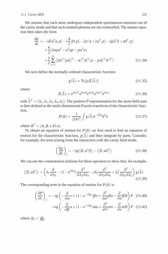
11.1 Cavity QED 223
We assume that each atom undergoes independent spontaneous emission out ofthe cavity mode and that such emitted photons are not reabsorbed. The master equa-tion then takes the form
dρdt
= −iδ [a†a,ρ ]− iΔ2
[D,ρ ]− i[ε∗a + εa†,ρ ]− ig[a†S + aS†,ρ ]
+κ2
(2aρa†−a†aρ−ρa†a)
+γ2
N
∑j=1
(2σ ( j)− ρσ ( j)
+ −σ ( j)+ σ ( j)
− ρ−ρσ ( j)+ σ ( j)
− ) (11.34)
We next define the normally ordered characteristic function
χ(�λ ) = Tr{ρΞ(�λ)} (11.35)
whereΞ(�λ ) = eiλ5S†
eiλ4Deiλ3Seiλ2a†eiλ1a (11.36)
with�λ T = (λ1,λ2,λ3,λ4,λ5). The positive P-representation for the atom-field stateis then defined as the multi-dimensional Fourier transform of the characteristic func-tion,
P(�α) =1
(2π)5
∫χ(�λ )e−i�λ�α d5λ (11.37)
where �αT = (α,β ,v,D,u).To obtain an equation of motion for P(�α) we first need to find an equation of
motion for the characteristic function, χ(�λ) and then integrate by parts. Consider,for example, the term arising from the interaction with the cavity field mode,
(dχdt
)I=−ig〈[Ξ ,a†S]〉− 〈[Ξ ,aS†]〉 (11.38)
We can use the commutation relations for these operators to show that, for example,
〈[Ξ ,aS†]〉=(
λ1∂
∂λ3− (1− e2iλ4)
∂ 2
∂λ2∂λ3− iλ5
∂ 2
∂λ2∂λ4+ λ 2
5∂ 2
∂λ2∂λ5
)χ(�λ)
(11.39)
The corresponding term in the equation of motion for P(�α) is
(∂P∂ t
)I= −ig
(− ∂
∂αv +(1− e−2∂D)β v +
∂ 2
∂u2 β u− ∂∂u
β D
)P (11.40)
+ig
(− ∂
∂βu +(1− e−2∂D)αu +
∂ 2
∂v2 αv− ∂∂v
αD
)P (11.41)
where ∂D = ∂∂D .

224 11 CQED
A problem is immediately apparent: this term contains infinite order derivativesand thus the resulting equation is not of Fokker–Planck form and does not define astochastic process. However a careful analysis shows that the exponential may betruncated to second order in an asymptotic expansion in N−1, which for N >> 1 isa reasonable approximation. The result after truncating is
∂P∂ t
= [−∂α [−iε− κα/2− igv]− ∂v[igαD− γv/2]
−∂D[−γ(D+ N)−2ig(uα− vβ )]+∂ 2
v [igαv]+ ∂ 2D[γ(D+ N)−2ig(uα− vβ )]+ CC
]P (11.42)
where CC stands for complex conjugate under the condition that v∗ �→ u,u∗ �→ v, α∗ �→ β , β ∗ �→ α . The corresponding stochastic differential equations are
α = −κα/2− iε− igv +Γα
β = −κ∗α/2 + iε + igv +Γβ
v = −γv/2 + igαD+Γv
u = −γ∗u/2− igβ D+Γu
D = −γ(D+ N)−2ig(αu−β v)+ΓD (11.43)
which should be compared to the single atom semiclassical equations to whichthey reduce when noise is neglected and we make the replacements β �→ α∗,u �→ v∗ N �→ 1. The only non-zero noise correlation functions are
〈Γv(t)Γv(t ′)〉 = 2igαv δ (t− t ′) (11.44)
〈Γu(t)Γv(t ′)〉 = 2igαu δ (t− t ′) (11.45)
〈ΓD(t)ΓD(t ′)〉 = 2γ(D+ N)−4ig(αu−β v)δ (t− t ′) (11.46)
These equations now provide a basis to obtain a phenomenological descriptionof optical bistability in terms of an intensity dependent cavity detuning. To pro-ceed we will assume that γ >> κ so that the atomic variables can be assumed toreach a steady state slaved to the instantaneous values of the field variables. Thisis called adiabatic elimination. The next step is to approximate the noise correla-tion functions for the atomic variables by replacing u,v by the steady state values ofthe deterministic equations for these variables. This is equivalent to a linearisationaround the deterministic steady state. The validity of this approximation rests onN >> 1. The resulting atomic variables are then substituted into the field equationsto give
α =−iε− κα/2− 2g2NαγΠ(αβ )
+Γ (t) (11.47)
where
Π(αβ ) = 1 +αβ
n0(1 + Δ 21)
(11.48)

11.2 Circuit QED 225
with n0 the saturation photon number and Δ1 as previously defined in (11.17 and11.18).
⟨Γ(t)Γ(t ′)
⟩=
κCx2
(1 + X + Δ21)3
[(1− iΔ1)3 +
X2
2
]δ (t− t ′)
⟨Γ†(t)Γ(t ′)
⟩=
κCx2
(1 + X + Δ21)3
[2X +
X2
2
]δ (t− t ′) (11.49)
with x = α/√
n0 and X = αβ/n0.
11.2 Circuit QED
Superconducting coplanar microwave cavities [13] enable a new class of experi-ments in circuit quantum electrodynamics in the strong coupling regime [14]. Thedipole emitter in this case is a single superconducting metalic island separated bytunnel junctions form a Cooper pair reservoir. Under appropriate conditions it ispossible for the charge on the island to be restricted to at most a single Cooper pair.This Cooper pair tunneling on an off the island constitutes a single large electricdipole system.
A possible experimental implementation is shown in Fig. 11.7.The coupling between a Cooper pair box charge system and the microwave field
of circuit QED is given by [13]
H = 4Ec ∑N
(N−ng(t))2|N〉〈N|− EJ
2 ∑N=0
(|N〉〈N + 1|+ |N + 1〉〈N|) (11.50)
ground
ground
V + V(t)
0
Cooper pair box
Vg
tunnel junctionsN = 0,1
Φ
Fig. 11.7 A co-planar microwave resonator is coupled to a Cooper pair box electric dipole

226 11 CQED
where
EC =e2
2CΣ
ng(t) =CgVg(t)
2e
with CΣ the capacitance between the island and the rest of the circuit, Cg is thecapacitance between the CPB island and the bias gate for the island, and Vg(t) is the
total voltage applied to the island by the bias gate composed of a DC field, V (0)g and
microwave field in the cavity, v(t). Thus we can write Vg(t) = V (0)g + v(t), where the
hat indicates a quantisation of the cavity field. Including the time dependent cavityfield we can write
ng(t) = n(0)g + δ ng(t) (11.51)
where
δ ng(t) =Cg
2ev(t) (11.52)
The Hamiltonian in (11.50) is written in the Cooper pair number basis. In thisbasis the electrostatic energy of the first term is quite clear. The Josephson energyterm describes tunneling of single Cooper pairs across the junction. This term ismore traditionally (i.e. in mean-field theory) written in the phase representation asEJ cosθ . The connection between these two representations is discussed in [15].
If the Cooper pair box is sufficiently small, the electrostatic charging energy isso large that it is very unlikely that there will be more than a single Cooper pair onthe island at any time. We can then usual restrict the CPB Hilbert space to N = 0,1,we can write the Hamiltonian as
H =−2EC(1−2n(0)g )σz− EJ
2σx−4ECδ ng(t)(1−2n(0)
g − σz) (11.53)
where σz = |0〉〈0−|1〉〈1|, σx = |1〉〈0|+ |0〉〈1|. Define the bare CPB Hamiltonianas
HCPB =−2EC(1−2n(0)g )σz− EJ
2σx (11.54)
and diagonalise it as
HCPB =ε2
σz (11.55)
where
ε =√
E2J +[4EC(1−2N(0)
g )]2 (11.56)
and now the Hamiltonian takes the form,
H = hωra†a +
ε2
σz−4ECδ ng(t)[1−2n(0)g − cosθσz + sinθσx] (11.57)
where we have now included the free Hamiltonian for the microwave cavity field,and

11.2 Exercises 227
θ = arctan
(EJ
4EC(1−2n(0)g )
)(11.58)
Operating at the charge degeneracy point, n(0)g = 1/2 so that θ = π/2, the
Hamiltonian becomes
H = hωca†a +ε2
σz−4ECCg
2ev(t)σx (11.59)
= hωca†a +ε2
σz− hg(a + a†)σx (11.60)
where the coupling constant is
hg = eCg
CΣ
√hωr
Lc(11.61)
This can be as large as 50 MHz[13]. The circuit resonance is typically at ωc ≈1 GHz. However, we can detune the qubit from this resonant frequency by afew MHz [14]. We can then make the rotating wave approximation and take theHamiltonian in the interaction picture to be the usual Jaynes–Cummings form
HI = hδaa†a + hg(aσ+ + a†σ−) (11.62)
with δa = ωc−ωb is the detuning between the cavity resonance and the CPB andhωb = ε .
Exercises
11.1 A laser may be modeled by the master equation in (11.34) with ε = 0 andwith the addition of the incoherent pump term
Lpρ =r2
N
∑j=1
(2σ ( j)+ ρσ ( j)
− −σ ( j)− σ ( j)
+ ρ−ρσ ( j)− σ ( j)
+ ) (11.63)
We will also assume that ωA = ωc
(a) Show that the Fokker-Planck equation is now given by
∂P∂ t
= [−∂α [−κα/
2− igv]− ∂v[igαD− γ‖v/
2]
−∂D[−γ‖(D−D0)−2ig(uα− vβ )]
+∂ 2v [igαv]−2r
∂ 2
∂v∂D+ NP
∂ 2
∂v∂u+∂ 2
D[r(N−D)+ γ(D+ N)−2ig(uα− vβ )+ CC]P (11.64)
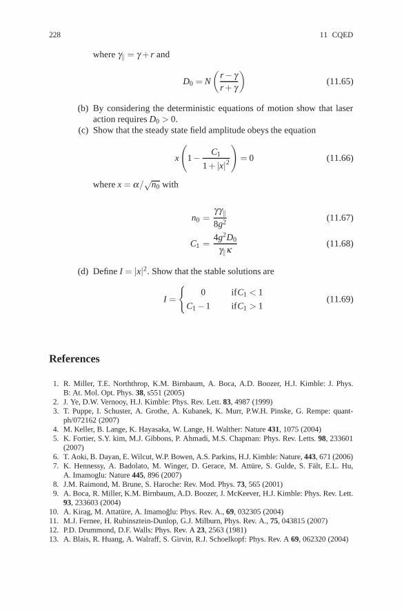
228 11 CQED
where γ‖ = γ + r and
D0 = N
(r− γr + γ
)(11.65)
(b) By considering the deterministic equations of motion show that laseraction requires D0 > 0.
(c) Show that the steady state field amplitude obeys the equation
x
(1− C1
1 + |x|2)
= 0 (11.66)
where x = α/√
n0 with
n0 =γγ‖8g2 (11.67)
C1 =4g2D0
γ‖κ(11.68)
(d) Define I = |x|2. Show that the stable solutions are
I =
{0 ifC1 < 1
C1−1 ifC1 > 1(11.69)
References
1. R. Miller, T.E. Norththrop, K.M. Birnbaum, A. Boca, A.D. Boozer, H.J. Kimble: J. Phys.B: At. Mol. Opt. Phys. 38, s551 (2005)
2. J. Ye, D.W. Vernooy, H.J. Kimble: Phys. Rev. Lett. 83, 4987 (1999)3. T. Puppe, I. Schuster, A. Grothe, A. Kubanek, K. Murr, P.W.H. Pinske, G. Rempe: quant-
ph/072162 (2007)4. M. Keller, B. Lange, K. Hayasaka, W. Lange, H. Walther: Nature 431, 1075 (2004)5. K. Fortier, S.Y. kim, M.J. Gibbons, P. Ahmadi, M.S. Chapman: Phys. Rev. Letts. 98, 233601
(2007)6. T. Aoki, B. Dayan, E. Wilcut, W.P. Bowen, A.S. Parkins, H.J. Kimble: Nature, 443, 671 (2006)7. K. Hennessy, A. Badolato, M. Winger, D. Gerace, M. Atture, S. Gulde, S. Falt, E.L. Hu,
A. Imamoglu: Nature 445, 896 (2007)8. J.M. Raimond, M. Brune, S. Haroche: Rev. Mod. Phys. 73, 565 (2001)9. A. Boca, R. Miller, K.M. Birnbaum, A.D. Boozer, J. McKeever, H.J. Kimble: Phys. Rev. Lett.
93, 233603 (2004)10. A. Kirag, M. Attature, A. Imamoglu: Phys. Rev. A., 69, 032305 (2004)11. M.J. Fernee, H. Rubinsztein-Dunlop, G.J. Milburn, Phys. Rev. A., 75, 043815 (2007)12. P.D. Drummond, D.F. Walls: Phys. Rev. A 23, 2563 (1981)13. A. Blais, R. Huang, A. Walraff, S. Girvin, R.J. Schoelkopf: Phys. Rev. A 69, 062320 (2004)

Further Reading 229
14. D.I. Schuster et al.: Nature 445, 515 (2007)15. J.F. Annett, B.L. Gyorffy, T.P. Spiller: Superconducting Devices for Quantum Computation.
In ‘Exotic States in Quantum Nanostructures’, S. Sarkar (ed.) (Kluwer Academic Publishers2002)
Further Reading
Haroche, S., J.M. Raimond: Exploring the quantum (Oxford University Press, Oxford, UK 2006)

Chapter 12Quantum Theory of the Laser
Abstract The quantum theory of the laser was developed in the 1960s principallyby the schools associated with H. Haken, W.E. Lamb and M. Lax, see [1, 2, 3, 4].Haken and Lax independently developed sophisticated techniques to convert opera-tor master equations into c-number Fokker–Planck equations or equivalent Langevinequations.
In this chapter we shall follow the approach of Scully and Lamb [3] to computephoton statistics and the linewidth of the laser. In the Scully–Lamb treatment thepumping is modelled by the injection of a sequence of inverted atoms into the lasercavity. In a usual laser, with a thermal pumping mechanism, a Poisson distributedsequence of inverted atoms is assumed. Introduction of a Bernoulli distribution en-ables a more general class of pumping mechanisms to be considered, including thecase of the regularly pumped laser. Diode lasers with more regular pumping thanusual lasers have recently been shown to give rise to sub-shot-noise photocurrentfluctuations.
12.1 Master Equation
A single mode cavity field is excited by a sequence of atoms injected into the cavity.Let ti be the arrival time of the atom i in the cavity and τ the time spent by each atomin the cavity. The change in the density operator for the field due to the interactionwith the ith atom may be represented by
ρ(ti + τ) = P(τ)ρ(ti) . (12.1)
The explicit form of P(τ) depends on the particular atomic system used in theexcitation process. The model we will employ is indicated in Fig. 12.1.
Of the four levels, only levels |1〉 and |2〉 are coupled to the intracavity field,which thus are referred to as the lasing levels. Each of these levels may then decay.Level |1〉 decays to level |3〉 at a rate γ1 while level |2〉 decays to level |4〉 at a rate γ2.
231

232 12 Quantum Theory of the Laser
Fig. 12.1 Schematic repre-sentation of the four-levelatomic model of a laser. Onlylevels 1 and 2 at coupled tothe laser field
We will assume that these decay rates are very much greater than the spontaneousdecay rate of level |2〉 to level |1〉, and thus we neglect spontaneous emission in thelasing levels. Each atom is prepared in the excited state |2〉 prior to interaction withthe cavity field. In the usual laser system the lifetimes γ−1
1 and γ−12 are much shorter
than the time τ spent by each atom in the cavity. This means that each atom rapidlyattains a steady state in passing through the cavity and the pump operation P(τ) iseffectively independent of the time τ . The effect of a single atom on the state of thefield may then be written as
ρ ′ = Pρ , (12.2)
where we have dropped the time dependence in ρ for simplicity, the prime servingto indicate the state of the field after the passage of a single atom through the cavity.We may represent the initial state of the field quite generally as
ρ =∞
∑n,m=0
ρn,m(0)|n〉〈m| . (12.3)
In Appendix [12.A] we solve the master equation for the system over the time τunder the assumptions discussed above. The result is
ρ ′ =∞
∑n,m=0
ρn,m(0)(Anm|n〉〈m|+ Bnm|n + 1〉〈m+ 1|) , (12.4)
where the explicit expressions for Anm, Bnm are given in the appendix.We now assume that each atom contributes independently to the field. (This as-
sumption remains valid even if there is more than one atom in the cavity at any time,provided that they are sufficiently dilute.) Thus, if k atoms are passed through thecavity from time 0 to time t the field density operator at time t is given by
ρ(t) = Pkρ(0) . (12.5)
More generally, however, not all atoms entering the cavity are prepared in the ex-cited state. Let the probability for an excited atom to enter the cavity between t andt + Δt be rΔt, r being the average injection rate. This defines a Poisson excitationprocess. Thus the field at time t +Δt is made up of a mixture of states correspondingto atomic excitation and no atomic excitation, thus
ρ(t + Δt) = rΔtPρ(t)+ (1− rΔt)ρ(t) . (12.6)

12.2 Photon Statistics 233
In the limit Δt→ 0 we havedρ(t)
dt= rU ρ(t) (12.7)
whereU = P−1 . (12.8)
We must now include the decay of the cavity field through the end mirrors. Thisis modelled in the usual way by coupling the field to a zero temperature heat bath.Thus the total master equation for the field density operator is
dρdt
= rU ρ +κ2
(2aρa†−a†aρ−ρa†a) , (12.9)
where κ is the cavity decay rate. This is the usual Scully–Lamb laser masterequation.
In the special case that γ1 = γ2 = γ the matrix elements of U in the number basisare greatly simplified. In this case the master equation in the number basis may bewritten as
dρnm
dt= G
( √nm
1 +(n + m)/2nsρn−1,m−1
− (m+ n + 2)/2 +(m−n)2/8ns
1 +(n + m+ 2)/2nsρnm
)
+κ2
[2√
(n + 1)(m+ 1)ρn+1,m+1− (n + m)ρnm] , (12.10)
whereG =
r2ns
(12.11)
and
ns =γ2
4g2 . (12.12)
where g is the coupling strength between the cavity and the levels 1 and 2.we have neglected terms ∝ n−2
s in the denominators of the first two coefficients.
12.2 Photon Statistics
The photon number distribution obeys the equation
dpn
dt=−G
(n + 1
1 +(n + 1)/nspn− n
1 +(n/ns)pn−1
)
+ κ(n + 1)pn+1−κnpn . (12.13)
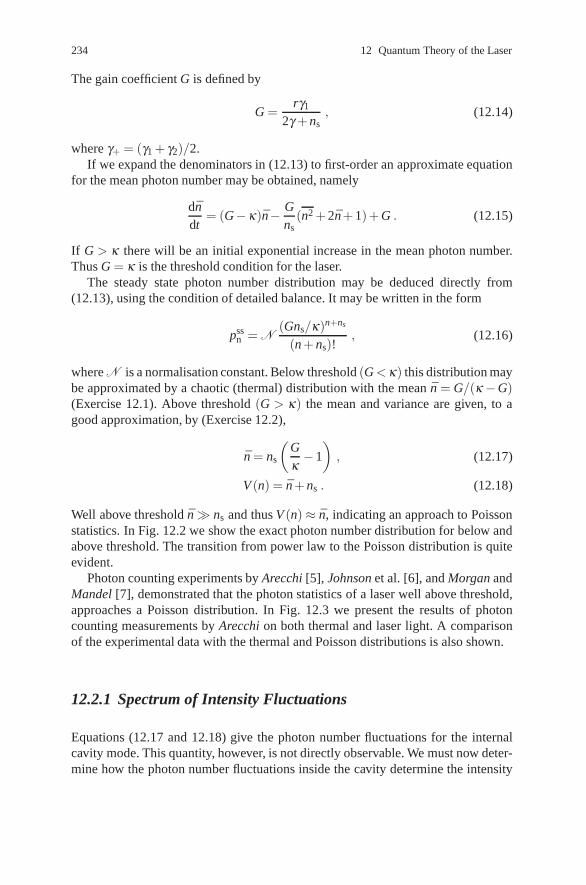
234 12 Quantum Theory of the Laser
The gain coefficient G is defined by
G =rγ1
2γ + ns, (12.14)
where γ+ = (γ1 + γ2)/2.If we expand the denominators in (12.13) to first-order an approximate equation
for the mean photon number may be obtained, namely
dndt
= (G−κ)n− Gns
(n2 + 2n+ 1)+ G . (12.15)
If G > κ there will be an initial exponential increase in the mean photon number.Thus G = κ is the threshold condition for the laser.
The steady state photon number distribution may be deduced directly from(12.13), using the condition of detailed balance. It may be written in the form
pssn = N
(Gns/κ)n+ns
(n + ns)!, (12.16)
where N is a normalisation constant. Below threshold (G < κ) this distribution maybe approximated by a chaotic (thermal) distribution with the mean n = G/(κ −G)(Exercise 12.1). Above threshold (G > κ) the mean and variance are given, to agood approximation, by (Exercise 12.2),
n = ns
(Gκ−1
), (12.17)
V (n) = n+ ns . (12.18)
Well above threshold n� ns and thus V (n)≈ n, indicating an approach to Poissonstatistics. In Fig. 12.2 we show the exact photon number distribution for below andabove threshold. The transition from power law to the Poisson distribution is quiteevident.
Photon counting experiments by Arecchi [5], Johnson et al. [6], and Morgan andMandel [7], demonstrated that the photon statistics of a laser well above threshold,approaches a Poisson distribution. In Fig. 12.3 we present the results of photoncounting measurements by Arecchi on both thermal and laser light. A comparisonof the experimental data with the thermal and Poisson distributions is also shown.
12.2.1 Spectrum of Intensity Fluctuations
Equations (12.17 and 12.18) give the photon number fluctuations for the internalcavity mode. This quantity, however, is not directly observable. We must now deter-mine how the photon number fluctuations inside the cavity determine the intensity

12.2 Photon Statistics 235
Fig. 12.2 The steady state photon number distribution of a laser operating above and below thresh-old. In (a) G/κ = 5.0, in (b) G/κ = 0.25. In both cases ns = 2
Fig. 12.3 Experimental results for the steady state photon number distribution for a thermal (i.e.Gaussian) light source and a laser operator above threshold. The laser exhibits Poissonian photonnumber statistics [5]

236 12 Quantum Theory of the Laser
fluctuations in the many mode field to which it is coupled through the output mir-rors. This is an application of the general input/output theory described in Chap. 7.
A single photoelectron detector placed at the output of the cavity measures aphotocurrent given by
i(t) = eξ 〈b†out(t)bout(t)〉 , (12.19)
where e is the electronic charge, and ξ = 2ε0cA/�ω with A the area of the detectorsurface. (We will assume unit quantum efficiency and unit amplification, for sim-plicity.) The output field bout(t) is related to the internal field and the input field by
bout(t) =√
κa(t)−bin(t) . (12.20)
We will assume the input field to be in the vacuum state. In that case
i(t) = eξ κ n , (12.21)
where n is the mean photon number inside the cavity.To determine the noise properties of the output field, the appropriate detector
quantity is i(0)i(τ). The theory of photo-electron detection (Chap. 3) enables this tobe related to the intensity fluctuations by
i(0)i(τ) = eξ 〈b†out(0)bout(0)〉δ (τ)+ e2ξ 2〈b†
out(0)bout(0)〉2+ e2ξ 2〈: I(0), I(τ) :〉 (12.22)
where : : denotes normal and time ordering and
I(τ) = b†out(τ)bout(τ). (12.23)
The first two terms in (12.22) represent a dc term and a δ -correlated shot-noise term.The last term carries information on a possible reduction in intensity fluctuations.We now define the normalised power spectrum
P(ω) =2
e2ξ 2
∞∫0
dτ cos(ωτ)i(0)i(τ) . (12.24)
Using (12.20) one may show that
〈: I(0), I(τ) :〉= κ2(〈a†(0)a†(τ)a(τ)a(0)〉− 〈a†(0)a(0)〉2) . (12.25)
Thusi(0)i(τ)
e2ξ 2 = κ n(1−κ n)+ κ nδ (τ)+ κ2g(τ) (12.26)
whereg(τ) = 〈a†(0)a†(τ)a(τ)a(0)〉 . (12.27)
We are only interested in the steady state fluctuations of the output field. In whichcase we can show that g(τ) = n2 and thus

12.3 Laser Linewidth 237
P(ω) = κ n . (12.28)
This flat photocurrent spectrum is the shot-noise limit of the laser.
12.3 Laser Linewidth
Well above threshold the laser produces Poisson photon statistics. A coherent statehas the same photon statistics, and this suggests that well above threshold the lasermight be producing a coherent state. This is not the case. While the intensity of thelaser is stabilised with a Poissonian distribution the phase of the laser undergoes adiffusion process. The effect of this phase diffusion is to cause a decay in the meanamplitude of the laser field, as the phase becomes uniformly distributed over 2π.The rate of amplitude decay Γ is thus a direct measure of the phase diffusion rate.
We will only discuss the case γ1 = γ2 = γ . The mean amplitude is defined by
〈a(t)〉=∞
∑n=0
n1/2ρn,n−1(t) . (12.29)
Using (12.10) we find
d〈a〉dt
=−G2
∞
∑n=0
(1/4ns)−11 +(2n + 1)/2ns
√nρn,n−1 . (12.30)
Assuming the laser operates well above threshold we can replace n by n in thedenominator of each coefficient. Then as n� ns
d〈a〉dt
=− G8n〈a〉 . (12.31)
Thus the phase diffusion rate is inversely proportional to the intensity of the laser.All second-order phase dependent correlation functions will decay at a similar rate.In particular, the two-time correlation function
F(τ) = 〈a†(τ)a(0)〉 (12.32)
will decay at the rate Γ = G/8n, i.e.
F(τ) = ne−Γτ . (12.33)
The Fourier transform of this function defines the laser spectrum
S(ω) =n
ω2 + Γ2 , (12.34)
and thus the laser linewidth is simply

238 12 Quantum Theory of the Laser
Γ =G8n
. (12.35)
It must be emphasised, however, that these results only apply well above threshold.
12.4 Regularly Pumped Laser
The Poissonian photon statistics of a laser reflect the contributions from the randompumping mechanism and spontaneous emission, which lead to an irregular photo-emission sequence. By suppressing the pump fluctuations, sub-Poissonian photonstatistics and thus sub-shot-noise photo-current fluctuations, are possible. This hasbeen demonstrated in recent experiments by Machida et al. [8] and also Richardsonand Shelby [9] with semiconductor lasers. The pump amplitude fluctuations werereduced by high impedance suppression of the electron injection rate.
We shall demonstrate how the Scully–Lamb laser theory can readily be modi-fied to incorporate regular pumping. Regular pumped lasers have been consideredtheoretically by a number of researchers [10, 11, 12, 13, 14]. We shall follow theapproach of Golubov and Sokolov [10], with some modifications.
Consider a time interval Δt short compared to the time scale on which the fieldis changing due to damping through the end mirrors. However, the time Δt is verylong compared to the time interval between successive pumping atoms entering thecavity. Divide the interval Δt into N steps of length τ . The probability for an excitedatom to enter the cavity at time t j = jτ is defined to be p. The fundamental proba-bilities of interest are then the probability of r excited atoms to enter the cavity atany of the N time steps, over the interval Δt. These probabilities are
Pr(Δt) =Δt(Δt− τ)(Δt−2τ) . . .(Δt− rτ)
τrr!
(p
1− p
)r
× exp
[Δtτ
ln(1− p)]
. (12.36)
To first order in Δt this is
Pr(t) = (−1)r+1(
p1− p
)r Δtrτ
. (12.37)
Between each atom entering the cavity the field evolves freely according to
T (τ) = e−iωaτa†aρe+iωaτa†a . (12.38)
The change in the state of the field due to the passage of a single atom is given by(12.4). It is a simple matter to prove that the operation describing the effect of thepump atoms P commutes with the free evolution operator T (if this is not the case

12.4 Regularly Pumped Laser 239
a simple master equation for the field state cannot be obtained in general). Thus thechange in the state of the field over a time Δt is
ρ(t + Δt) = T (Δt)
[N
∑n=0
Pn(Δt)Pnρ(t)
](12.39)
(i.e., we can factor out the free evolution between each time step). We henceforthassume we are working in the interaction picture and drop the free evolution term.As we assume τ � Δt we extend the upper limit on the sum to ∞, then
ρ(t + Δt) = ρ(t)+Δtτ
ln(1− p)ρ(t)
+Δtτ
[p
1− pP− 1
2
(p
1− p
)2
P2 + . . .
]ρ(t) . (12.40)
From which we obtain
dρdt
=1τ
ln(1− p)ρ(t)+1τ
ln
(1 +
p1− p
P
)ρ(t) (12.41)
= R ln(1 + pU )ρ(t) , (12.42)
where R = τ−1 is the pumping rate for a perfectly regular process (p = 1) and
U = P−1 . (12.43)
We can define an average injection rate r = pR, then
dρdt
=rp
ln(1 + pU )ρ(t) . (12.44)
In this form we can take the Poisson limit defined by p→ 0, R→ ∞, such thatpR = constant = r. In this limit the equation reduces to that for a normal laser.
The difficulty in discussing the regularly pumped laser is the logarithm term in(12.42). As U represents the change in the state of the field due to a single atomwe might expect U to be in some sense small. With this in mind we expand thelogarithm to second order. Unfortunately this leads to a rather pathological masterequation. However, the procedure does give accurate results for the first-and second-order moments of the photon number.
The photon number distribution now obeys the equation
dpn
dt= κ [−npn +(n + 1)pn+1]+ r(−an+1Pn + anpn−1)
+pr2
[−a2n+1pn + an(an + an+1)pn−1−anan−1 pn−2] , (12.45)

240 12 Quantum Theory of the Laser
where
an =Gn
r(1 +(n/ns)). (12.46)
To obtain the stationary state variances is a rather more difficult process than for thePoisson pumped case. The mean photon number above threshold is not changed,however the variance is given by
V (n) = n
(1− pγ1
2(γ1 + γ2)
)+ ns . (12.47)
We consider some special cases of this result for regular pumping, p = 1. Farabove threshold n� ns so we may neglect the last term in (12.47). When the decayrates are equal, the photon number variance is
V (n) =3n4
(γ1 = γ2) . (12.48)
In this case spontaneous emission from level |2〉 is contributing to the noise. Thiseffect may be reduced by increasing the decay rate of the lower level with respect tothe upper level, γ1� γ2. In this case
V (n) =n2(γ1� γ2) . (12.49)
Thus the width of the photon number distribution inside the cavity is reducedby half.
We now consider intensity fluctuations of the light emerging from the cavity. Wemay obtain a solution for the normally ordered two-time correlation function g(τ),from the master equation (12.45) assuming a Gaussian steady state distribution. Theresult is
g(τ) = n2 +[V (n)− n]e−δτ , (12.50)
where
δ = κn/ns
1 +(n/ns). (12.51)
Substituting (12.47 and 12.50) into (12.26) the spectrum of the photocurrent fluctu-ations is given by
P(ω) = κ n
(1 +
2κQδω2 + δ 2
), (12.52)
where
Q =V (n)− n
n(12.53)
=− pγ1
2(γ1 + γ2)+
ns
n. (12.54)

12.4 Regularly Pumped Laser 241
The Q parameter measures the deviation of the intracavity field from Poisson statis-tics. In the limit of regular pumping (p = 1) and far above threshold
P(ω) = κ n
(1− γ1κ2
(γ1 + γ2)(κ2 + ω2)
). (12.55)
Thus at cavity resonance (ω = 0),
P(0) = κ n(1 + 2Q)
= κ nγ1
γ1 + γ2. (12.56)
The first term in the first equation represents the shot-noise contribution. A negativevalue of Q leads to a reduction below the shot-noise limit. If the decay rates areequal (γ1 = γ2), spontaneous emission is not suppressed and
P(0) =κ n2
, (12.57)
which represents a 50% reduction below the shot-noise level. However, in the limitγ1� γ2, Q approaches – 0.5 far above threshold and
P(ω) = κ n
(1− κ2
κ2 + ω2
). (12.58)
Then at cavity resonance, the fluctuation spectrum is zero. This may be comparedwith the light inside the cavity where the photon number fluctuations were onlyreduced by one half. This result has the same interpretation as the limit to theintracavity squeezing in a parametric oscillator; there is a destructive interferencefrom the vacuum fluctuations reflected from the cavity mirror and the reduced noiselight emerging from the cavity. This results in no fluctuations in the output light onresonance.
In Fig. 12.4 we show the results of the experiment by Machida et al. [8] for aregularly pumped semiconductor laser.
Fig. 12.4 The normalisedamplitude noise level versusthe pump rate for a laser withpump noise (dashed) andwith pump noise suppressed(solid) [11]

242 12 Quantum Theory of the Laser
12.A Appendix: Derivation of the Single-Atom Increment
Consider a single multilevel atom (Fig. 12.1) prepared in the state |2〉. Level |1〉 isdamped at the rate γ1 to level |3〉 and level |2〉 is damped at the rate γ2 to level |4〉.Only levels |1〉 and |2〉 interact with the cavity field. The master equation describingthe dynamics of this system is
dρdt
=ig[a†σ12− + aσ12
+ ,ρ ]
+γ1
2(2σ13
− ρσ13+ −σ13
+ σ13− ρ−ρσ13
+ σ13− )
+γ2
2(2σ24
− ρσ24+ −σ24
+ σ24− ρ−ρσ24
+ σ24− ) (12.59)
(we ignore spontaneous emission on the lasing levels |1〉, |2〉). We will present acomplete operator solution to the master equation over the time τ and then considerthe limit γiτ� 1.
Define the operation
J ρ = γ1σ13− ρσ13
+ + γ2σ24− ρσ24
+ (12.60)
and the rate operator
R = γ1σ13+ σ13
− + γ2σ24+ σ24
− (12.61)
= γ1|1〉〈1|+ γ2|2〉〈2| . (12.62)
The solution to the master equation may then be written formally
ρ(t) =S (t)ρ(0)+t∫
0
dt1S (t− t1)J S (t1)ρ(0)
+t∫
0
dt1
t1∫0
dt2S (t− t1)J S (t1− t2)J S (t2)ρ(0)
+ · · · , (12.63)
whereS (t)ρ = B(t)ρB†(t) , (12.64)
withB(t) = exp[−ig(a†σ12
− + aσ12+ )− γ1t|1〉〈1|− γ2t|2〉〈2|] . (12.65)
For
ρ(0) = |2〉〈2|⊗ρF(0) (12.66)
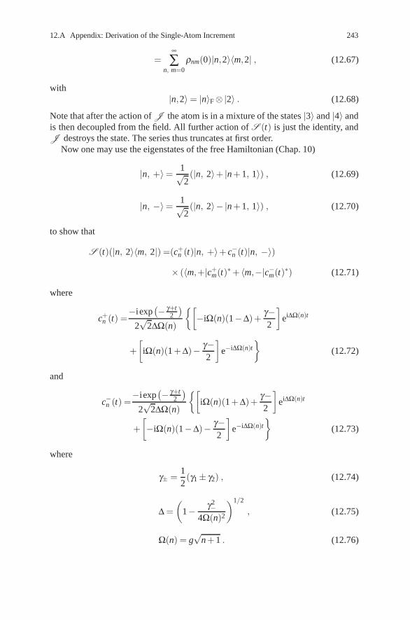
12.A Appendix: Derivation of the Single-Atom Increment 243
=∞
∑n, m=0
ρnm(0)|n,2〉〈m,2| , (12.67)
with|n,2〉= |n〉F⊗|2〉 . (12.68)
Note that after the action of J the atom is in a mixture of the states |3〉 and |4〉 andis then decoupled from the field. All further action of S (t) is just the identity, andJ destroys the state. The series thus truncates at first order.
Now one may use the eigenstates of the free Hamiltonian (Chap. 10)
|n, +〉= 1√2(|n, 2〉+ |n + 1, 1〉) , (12.69)
|n, −〉= 1√2(|n, 2〉− |n + 1, 1〉) , (12.70)
to show that
S (t)(|n, 2〉〈m, 2|) =(c+n (t)|n, +〉+ c−n (t)|n, −〉)
× (〈m,+|c+m(t)∗+ 〈m,−|c−m(t)∗) (12.71)
where
c+n (t) =
−iexp(− γ+t
2
)2√
2ΔΩ(n)
{[−iΩ(n)(1−Δ)+
γ−2
]eiΔΩ(n)t
+[
iΩ(n)(1 + Δ)− γ−2
]e−iΔΩ(n)t
}(12.72)
and
c−n (t) =−iexp
(− γ+t2
)2√
2ΔΩ(n)
{[iΩ(n)(1 + Δ)+
γ−2
]eiΔΩ(n)t
+[−iΩ(n)(1−Δ)− γ−
2
]e−iΔΩ(n)t
}(12.73)
where
γ± =12(γ1± γ2) , (12.74)
Δ =(
1− γ2−4Ω(n)2
)1/2
, (12.75)
Ω(n) = g√
n + 1 . (12.76)

244 12 Quantum Theory of the Laser
We now assume γ1, 2t � 1. The first term in (12.63) may be ignored as it simplydecays to zero.
We are interested in the state of the field alone which is obtained by tracing outover the atomic states. We use
TrA(J S (t)|n, 2〉〈m, 2|) =γ2
2|n〉〈m|[c+
n (t)+ c−n (t)][c+m(t)∗+ c−m(t)∗]
+γ1
2|n + 1〉〈m+ 1|[c+
n (t)− c−n (t)]
× [c+m(t)∗ − c−m(t)∗] . (12.77)
Thus we obtain in the steady state, the single atom increment
ρ ′ =∞
∑n, m=0
ρnm(0)(Anm|n〉〈m|+ Bnm|n + 1〉〈m+ 1|) , (12.78)
where
Anm =γ2
2
∞∫0
dt[c+n (t)+ c−n (t)][c+
m(t)∗+ c−m(t)∗] , (12.79)
Bnm =γ1
2
∞∫0
dt[c+n (t)− c−n (t)][c+
m(t)∗ − c−m(t)∗] . (12.80)
Note that Tr(ρ) = 1 requires that Ann + Bnn = 1. We quote only the results for thediagonal matrix elements,
Ann =(
γ2
2γ+
)4Ω(n)2 + 2γ1γ+
4Ω(n)2 + γ1γ2(12.81)
and
Bnn = 1−Ann =(
γ2
2γ+
)4Ω(n)2
4Ω(n)2 + γ1γ2. (12.82)
To compute the change in the state we write
ρ ′ = (1 +U )ρ = Pρ . (12.83)
The diagonal matrix elements of U ρ are then found to be
〈n|U ρ |n〉=−an+1 pn + anpn+1 , (12.84)
wherean+1 = Ann−1 . (12.85)

References 245
Exercises
12.1 Show that below threshold (G < κ) the master equation may be approxi-mated by
dρdt
=G2
(2a†ρa−aa†ρ−ρaa†)+ κ(2aρa†−a†aρ−ρa†a) .
Thus demonstrate that the steady state density operator is
ρ ss =(
1− Gκ
) ∞
∑n=0
(Gκ
)n
|n〉〈n| (12.86)
which is equivalent to a chaotic state.12.2 Show that well above threshold the laser master equation may be approxi-
mated by
dρdt
=Gns
2(2n−1/2a†ρan−1/2−an−1a†ρ−ρan−1a†)
+κ2
(2aρa†−a†ρa−ρa†a)
where n = a†a. Show that the steady-state solution is
ρ ss = exp
(−Gns
κ
) ∞
∑n=0
(Gns/κ)n
n!|n〉〈n| . (12.87)
12.3 Show that the contours of the Q-function for the laser steady states in Exer-cises 12.1, 12.2 are: (a) Circles centred on the origin for below threshold, (b)annulli centered at the radius r = (Gns/κ)1/2, for the above threshold state.Thus in both cases the phase of the field is random.
References
1. H. Haken: Laser Theory, Reproduction from Handbuch der Physik (Springer, Berlin,Heidelberg 1984)
2. M. Sargent III, M.O. Scully, W.E. Lamb: Laser Physics (Addison Wesley 1974)3. M.O. Scully, W.E. Lamb: Phys. Rev. 159, 208 (1967)4. M. Lax, W.H. Louisell: Phys. Rev. 185, 568 (1969)5. F.T. Arecchi: Phys. Rev. Lett. 15, 912 (1965)6. E.A. Johnson, R. Jones, T.P. McLean, E.R. Pike: Phys. Rev. Lett. 16, 589 (1966)7. B.L. Morgan, L. Mandel: Phys. Rev. Lett. 16, 1012 (1966)8. S. Machida, Y. Yamamoto, Y. Itaya: Phys. Rev. Lett. 58, 1000 (1987)

246 12 Quantum Theory of the Laser
9. W. Richardson, R.E. Shelby: Phys. Rev. Lett. 64, 400 (1990)10. Y.M. Golubov, I.V. Sokolov: Sov. Phys. JETP 60, 234 (1984)11. Y. Yamamoto, S. Machida, O. Nilsson: Phys. Rev. A 34, 4025 (1986)12. F. Haake, S.M. Tan, D.F. Walls: Phys. Rev. A 40, 7121 (1989)13. J. Bergou, L. Davidovich, M. Orszag, C. Berkert, M. Hillery, M.O. Scully: Opts. Commun.
72, 82 (1989)14. M. Marte, P. Zoller: Quantum Optics 2, 229 (1990)

Chapter 13Bells Inequalities in Quantum Optics
Abstract The early days of quantum mechanics were characterised by debates overthe applicability of established classical concepts, such as position and momentum,to the new formulation of mechanics. The issues became quite distinct in the pro-tracted exchange between A. Einstein and N. Bohr, culminating in the paper ofEinstein, Podolsky and Rosen (EPR) in 1935 [1]. Bohr, in his response to this pa-per, [2] expanded upon his concept of complementarity and showed that the EPRargument did not establish the incompleteness of quantum mechanics, as EPR hadclaimed, but rather highlighted the inapplicability of classical modes of descriptionin the quantum domain. A. Einstein, however, did not accept this position and thetwo sides of the debate remained unreconciled, while most physicists generally be-lieved that N. Bohr’s argument carried the day.
Thus the matter rested until 1964 when J.S. Bell opened up the possibility ofdirectly testing the consequences of the EPR premises. We will discuss the EPRargument and the analysis of Bell in the context of correlated photon states.
13.1 The Einstein–Podolsky–Rosen (EPR) Argument
The essential step in the EPR argument is to introduce correlated pure states of twoparticles (or photons) of the form
|Ψ〉= ∑n|an〉1⊗|bn〉2 , (13.1)
where {|an〉1} and {|bn〉2} are ortho-normal eigenstates for some operators A1 andB2 of particles 1 and 2, respectively. The correlations between the particles persisteven if in the course of the experiment the particles become spatially separated afterthe interaction responsible for the correlated state.
Now suppose one were to measure the operator A1 on particle one long after theinteraction between the particles has ended, and the two particles are far apart. If theresult is some eigenvalue an, particle 1 must thence-forth be considered to be in the
247
248 13 Bells Inequalities in Quantum Optics
state |an〉1, while particle 2 must be in the state |bn〉2. As the state of particle 2 is nowan eigenstate of B2 we can predict with probability one that the physical quantityrepresented by B2 if measured will give the result bn. Thus we can predict the valueof this physical quantity for particle 2 without in any way interacting with it.
Suppose, however, that instead of measuring A1 on particle 1 we measured someother quantity, C1, with eigenstates |cn〉1. We then rewrite the state in (13.1) as
|Ψ〉= ∑n|cn〉1⊗|dn〉2 , (13.2)
where |dn〉2 is an eigenstate of some other operator D2 for particle 2. If the result cn
is obtained for the measurement on particle 1, particle 2 must be in the state |dn〉2for which a measurement of D2 must give the result dn. Thus depending on whatwe choose to measure on particle 1 the state of particle 2 after the measurement,can be an eigenstate of two quite different operators. This is another example of themeasurement ambiguity discussed in the previous chapter. However, the EPR argu-ment now raises one very important question. Is it possible that the two operatorson particle 2, B2 and D2, do not commute? If this were the case the EPR argumentestablishes that, depending on what is measured on particle 1, we can predict withcertainty the values of physical quantities, represented by noncommuting operatorswithout in anyway interacting with this particle. By explicit construction Einstein,Podolsky and Rosen showed that this is indeed possible.
EPR claimed that “if without in anyway disturbing a system, we can predict withcertainty (i.e., with probability equal to unity), the value of a physical quantity, thenthere exists an element of physical reality corresponding to that quantity”.
Assuming that the wave function does contain a complete description of the two-particle system it would seem that the argument of EPR establishes that it is possibleto assign two different states (|bn〉2 and |dn〉2) to the same reality. However, in thelanguage of EPR, two physical quantities represented by operators which do notcommute cannot have simultaneous reality. The conclusion of EPR was that thequantum mechanical description of physical reality given by the wave function isnot complete.
13.2 Bell Inequalities and the Aspect Experiment
Were one to adopt the conclusion of EPR it would seem necessary to search for amore complete physical theory than quantum mechanics. To obtain such a theory,quantum mechanics should be supplemented by additional, perhaps inaccessible,variables. As Bell [3] showed, attempting to complete the theory in this way andmaintain the locality condition (that measurements on particle 1 carried out whenthe particles are spatially separated should have no effect on particle 2) leads tostatistical predictions which differ from those of standard quantum theory.
To elucidate Bell’s argument we consider a system in which correlated photonpolarisation states are produced. Such a system is the (J = 0)→ (J = 1)→ (J = 0)

13.2 Bell Inequalities and the Aspect Experiment 249
Fig. 13.1 Schematic representation of the experiment of Aspect et al. [4] to test quantum mechanicsagainst the Bell inequality. S is a source of two polarised photons. 1 and 2 label polarisationanalysers, with orthogonal output channels labelled + and −. The polarisation analysers are set atangles θ1, θ2
cascade two-photon transition in calcium-40 (Fig. 13.1). The two photons are emit-ted in opposite directions (by conservation of momentum) with correlated polari-sation states. Each photon passes through separate polarisation analysers, emergingin either the horizontal (+) channel, or the vertical channel (−) of each analyser.Initially let us assume that the horizontal polarisation is chosen to be orthogonal tothe plane of the experiment and that both analysers are so aligned. However, we arefree to rotate the polarisers in the plane orthogonal to the propagation direction ofthe photons. We follow the treatment of Reid and Walls [5].
Let a±(b±) be the annihilation operator for the horizontally (+) or vertically(−) polarised mode for the field travelling to analyser 1 (labelled 1) or analyser 2(labelled 2). The state of the two photons may be written as
|Ψ〉= 1√2(a†
+b†+ + a†
−b†−)|0〉 , (13.3)
where |0〉 is the vacuum state. Using the notation |n1, n2, n3, n4〉 to denote n1
photons in mode a+, n2 photons in mode a−, n3 photons in mode b+ and n4 photonsin mode b−, the state may be expressed as
|ψ〉= 1√2(|1,0,1,0〉+ |0,1,0,1〉) . (13.4)
If the photon in analyser 1 is detected in the (+) channel, the state of the photondirected towards 2 must be polarised in the horizontal direction. This correlation isthus precisely of the kind required for the EPR experiment.
We are free to measure the polarisation in any direction by rotating the analysersthrough the angles θ1 and θ2 for detector 1 and 2, respectively. The detected modesin this case are orthogonal transformations of the modes a± and b±;
c+ = a+ cosθ1 + a− sinθ1 , (13.5a)
c− =−a+ sinθ1 + a− cosθ1 , (13.5b)
d+ = b+ cosθ2 + b− sinθ2 , (13.5c)
d− =−b+ sinθ2 + b− sinθ2 . (13.5d)

250 13 Bells Inequalities in Quantum Optics
The detectors placed after the polarisers measure the intensities 〈I±1 〉 and 〈I±2 〉,while the correlators measure 〈I+
1 I+2 〉, etc. In fact, for the two-photon state 〈I±i 〉 =
P±i , is the probability for one count in the + or − channel of detector i. Of course,these moments depend on θ1 and θ2. Let us further suppose that in a complete theorythese functions also depend on the variable λ which remains hidden from directdetermination and for which only a statistical description is available. This variableis distributed according to some density ρ(λ ). In general, we may then write
〈I±1 I±2 〉θ1θ2 =∫
ρ(λ )I±1 (λ ,θ1,θ2)I±2 (λ ,θ1,θ2)dλ , (13.6)
where I+1 denotes the expected intensity at detector 1 given a value for λ , namely
I+1 (λ ,θ1,θ2) =
∫I+1 ρ(I+
1 |λ ,θ1,θ2)dI+1 . (13.7)
It is reasonable to assume, as in EPR, that for a given value of λ the results at 1cannot depend on the angle θ2 chosen at 2, (and conversely). This is the “localityassumption”, it is formally represented by
I±1 (λ ,θ1,θ2) = I±1 (λ ,θ1) , (13.8a)
I±2 (λ ,θ1,θ2) = I±2 (λ ,θ2) . (13.8b)
Consider the following correlation functions:
E(θ1,θ2) =〈(I+
1 − I−1 )(I+2 − I−2 )〉
〈(I+1 + I−1 )(I+
2 + I−2 )〉 . (13.9)
In terms of the detected mode operators this may be written in the form
E(θ1,θ2) =〈: (c†
+c+− c†−c−)(d†
+d+−d†−d−) :〉
〈: (c†+c+ + c†
−c−)(d†+d+ + d†
−d−) :〉 (13.10)
where : : denotes normal ordering.Assuming a local hidden variable theory we may write
E(θ1,θ2) = N−1∫
f (λ )S1(λ ,θ1)S2(λ ,θ2)dλ , (13.11)
where
S1(λ ,θ1) =I+1 (λ ,θ1)− I−1 (λ ,θ1)
I1(λ ), (13.12)
S2(λ ,θ1) =I+2 (λ ,θ2)− I−2 (λ ,θ2)
I2(λ ), (13.13)

13.2 Bell Inequalities and the Aspect Experiment 251
f (λ ) = ρ(λ )I1(λ )I2(λ ) (13.14)
with
I1(λ ) = I+1 (λ ,θ1)+ I−1 (λ ,θ2) , (13.15a)
I2(λ ) = I+2 (λ ,θ2)+ I−2 (λ ,θ2) . (13.15b)
The latter equations correspond to the intensity of light measured at 1 or 2 with thepolarisers removed. The normalisation N is
N =∫
f (λ )dλ . (13.16)
The functions |S1(λ ,θ1)| and |S2(λ ,θ2)| are bounded by unity:
|S1(λ ,θ1)| ≤ 1 , (13.17a)
|S2(λ ,θ2)| ≤ 1 . (13.17b)
To obtain a testable statistical quantity we need to consider how E(θ1,θ2)changes as the orientation of the polarisers are changed. With this in mind, con-sider E(θ1,θ2)−E(θ1,θ ′2). This quantity may be expressed as
E(θ1,θ2)−E(θ1,θ ′2) = N−1∫
dλ f (λ )S1(λ ,θ1)S2(λ ,θ2)[1±S1(λ ,θ ′1)S2(λ ,θ ′2)]
−N−1∫
dλ f (λ )S1(λ ,θ1)S2(λ ,θ ′2)
× [1±S1(λ ,θ ′1)S2(λ ,θ2)] . (13.18)
Then using (13.17a and b)
|E(θ1,θ2)−E(θ1,θ ′2)| ≤ N−1∫
dλ f (λ )[1±S1(λ ,θ ′1)S2(λ ,θ ′2)]
+ N−1∫
dλ f (λ )[1±S1(λ ,θ ′1)S2(λ ,θ2)]
= 2± [E(θ ′1,θ′2)+ E(θ ′1,θ2)].
Finally, we obtain the Bell inequality
|B| ≤ 2 , (13.19)
whereB = E(θ1,θ2)−E(θ1,θ ′2)+ E(θ ′1,θ
′2)+ E(θ ′1,θ2) .
This particular Bell inequality is known as the Clauser–Horne–Shimony–Holt(CHSH) inequality.
As we shall see, there are states of the field which violate the inequality equa-tion (13.19) [for example, the state given in (5)]. We note firstly, however, that if the
252 13 Bells Inequalities in Quantum Optics
state of the field can be represented by a positive, normalisable Glauber–SudarshanP-representation no violation of this inequality is possible. Let α = (α+,α−,β+,β−)be the c-number corresponding to the modes a±,b±. If we define the following‘transformation’ variables for the modes c±,d±,
γ+ = α+ cosθ1 + α− sinθ1, δ+ = β+ cosθ2 + β− sinθ2,
γ− =−α+ sinθ1 + α− cosθ1, δ− =−β+ sinθ2 + β− cosθ2 , (13.20)
the correlation function E(θ1,θ2) becomes
E(θ1,θ2) = N−1∫
P(α)(|γ+|2−|γ−|2)(|δ+|2−|δ−|2)d2α (13.21)
withN =
∫P(α)(|γ+|2 + |γ−|2)(|δ+|2 + |δ−|2)d2α .
Recalling that the transformations in (13.20) are orthogonal we note that
|γ+|2 + |γ−|2 = |α+|2 + |α−|2 and |δ+|2 + |δ−|2 = |β+|2 + |β−|2
the normalisation may be written
N =∫
P(α)(|α+|2 + |α−|2)(|β+|2 + |β−|2)d2α , (13.22)
where the integrand does not depend on θ1 or θ2. Then
E(θ1,θ2) = N−1∫
P(α)(|α+|2 + |α−|2)(|β+|2 + |β−|2)S(γ)S(δ ) , (13.23)
where
S(γ) =|γ+|2−|γ−|2|α+|2 + |α−|2 (13.24)
and
S(δ ) =|δ+|2−|δ−|2|β+|2 + |β−|2 . (13.25)
As S(γ) is a function of θ1 and not θ2 while S(δ ) is a function of θ2 and not θ1,the Glauber–Sudarshan representation is local. It then follows immediately that pro-vided P(α) is positive and normalisable, the Bell inequality in (13.19) must hold.
The correlation function E(θ1,θ2) may be evaluated directly for the state in(13.4) using the normally-ordered moment in (13.9). One finds
E(θ1,θ2) = cos2ψ , (13.26)

13.2 Bell Inequalities and the Aspect Experiment 253
whereψ ≡ θ1−θ2 .
If we choose
ψ = θ2−θ1 = θ ′1−θ2 = θ ′1−θ ′2 =13(θ1−θ ′2) ,
one findsB = 3cos2ψ− cos6ψ . (13.27)
When ψ = 22.5◦, B = 2√
2 showing a clear violation of the Bell inequality |B| ≤ 2.This violation has convincingly been demonstrated in the experiment of
Aspect [4]. In this experiment the polarisation analysers were essentially beam split-ters with polarisation-dependent transmittivity. Ideally, one would like to have thetransmittivity (T +) for the modes a+ and b+ equal to one, and the reflectivity (R−)for the modes a− and b− also equal to one. However, in the experiment the mea-sured values were T +
1 = R−1 = 0.950, T−1 = R+1 = 0.007 and T +
2 = T−2 = 0.930,T−2 = R+
2 = 0.007.The expression for E(θ1,θ2) is then modified:
E(θ1,θ2) = F(T+
1 −T−1 )(T +2 −T−2 )
(T+1 + T−1 )(T +
2 + T−2 )cos2ψ , (13.28)
where F is a geometrical factor accounting for finite solid angles of detection. In thisexperiment F = 0.984, and quantum mechanics would give for ψ = 22.5◦, B = 2.7.
The observed value was 2.697± 0.015, in quite good agreement with quantumtheory and a clear violation of the Bell inequality. In Fig. 13.2 is shown a plot ofthe theoretical and experimental results as a function of ψ . The agreement withquantum mechanics is better than 1%. It would appear in the light of this experimentthat realistic local theories for completing quantum mechanics are untenable.
Fig. 13.2 Correlation ofpolarisations as a functionof the relative angle of thepolarisation analysers. Theindicated errors are ±2 stan-dard deviations. The dot-ted curve is the quantum-mechanical prediction for theexperiment. For ideal polaris-ers the curves woudl reachthe values ±1. (From Aspectet al. Phys. Rev. Letts. 49,92 (1982))

254 13 Bells Inequalities in Quantum Optics
13.3 Violations of Bell’s Inequalities Using a ParametricAmplifier Source
The Bell inequality presented in (13.19) is only one of a large class of inequalitiesviolated by quantum mechanics. Another inequality has recently been tested by Ouand Mandel [6] based on an experiment first suggested by Reid and Walls [5]. Ithas now been realised in a number of configurations [7, 8]. We shall discuss the Ouand Mandel experiment presented schematically in Fig. 13.3. A parametric downconverter produces two beams of linearly polarized signal and idler photons. Phasematching conditions give a relative angle of 4◦ between the propagation direction ofthe two beams. The idler photons pass through a 90◦ polarization rotator. The signaland idler beams are then incident from opposite sides onto a beam splitter. After thebeam splitter, the two beams now consisting of mixed signal and idler photons passthrough linear polarizers set at adjustable angles θ1 and θ2 before falling on twophotodetectors. The coincidence counting rate of the two detectors is then measuredwith a time-to-digital converter. This provides a measure of the joint probability ofdetecting two photons for various settings θ1 and θ2 of the two polarizers.
In this experiment the polarisation analysers used have only a single output chan-nel. However, we can still derive a Bell inequality violated by quantum mechanics.If we define the correlation function P(θ1,θ2) by
P(θ1,θ2) = 〈I1I2〉θ1θ2 (13.29)
the following Bell inequality may be derived as
Fig. 13.3 Schematic representation of the experiment of Ou and Mandel to test the CHSH inequal-ity using parametric down conversion [9]

13.3 Violations of Bell’s Inequalities Using a Parametric Amplifier Source 255
S = P(θ1,θ2)−P(θ1,θ ′2)+ P(θ ′1,θ′2)+ P(θ ′1,θ2)
−P(θ1,−)−P(−,θ2)≤ 0 , (13.30)
where
P(θ1,−) = 〈I1I2〉θ1 , (13.31)
P(−,θ2) = 〈I1I2〉θ2 (13.32)
are the intensity correlation functions with one or the other polariser removed. Theinequality in (13.30) is known as the Clauser–Horne inequality. Just as in the case ofthe CHSH inequality (13.19) this inequality is satisfied for states of the field whichcan be represented by a positive, normalisable Glauber–Sudarshan P-representation[5]. It may, however, be violated for certain quantum fields.
We follow closely the treatment given by Tan and Walls [9]. We now proceedto calculate P(θ1,θ2) and S for the experiment of Ou and Mandel [6]. We includethe possibility of placing an attenuator in the idler beam. Let a+ and a− denote theannihilation operators for the x and y polarized modes in the idler beam, and let b+and b− denote the operators for the corresponding modes in the signal beam. Theoutgoing modes from the beam splitter are described by the operators c± and d±,and obey the following relationships:
c+ =√
T+b+ + i√
R+a+,
c− =√
T−b−− i√
R−a−,
d+ =√
T+a+ + i√
R+b+,
d− =√
T−a−− i√
R−b− , (13.33)
where T± and R± are the intensity transmission and reflection coefficients for the xand y polarizations. The phase relationships arise from the Fresnel formula. Sincethe signal beam is polarized in the x direction, and the idler beam is polarized in they direction, the modes associated with the operators a+ and b+ are the annihilationoperators for the output modes of the parametric down converter. When an atten-uator with the intensity transmission coefficient η is placed in the idler beam, theoperators a− in the above equations is replaced by
√ηa−+
√1−ηυ , (13.34)
where the vacuum mode operator υ is included to give the correct level of fluctua-
tions in the attenuated beam. Photodetectors 1 and 2 respond to the fields E(+)1 and
E(+)2 , respectively, where

256 13 Bells Inequalities in Quantum Optics
E(+)1 = c+ cosθ1 + c− sin θ1,
E(+)2 = d+ cosθ2 + d− sinθ2 , (13.35)
The joint two-photon detection probability (for perfect detector efficiency) is
P(θ1,θ2) = 〈ψ |E(−)1 E(−)
2 E(+)2 E(+)
1 |ψ〉 . (13.36)
For low conversion efficiencies the output of the parametric down converter is a pairof photons, one in each of the signal and idler modes a− and b+. Thus |ψ〉= |1,1〉,this yields
P(θ1,θ2) = η(√
R+R− sinθ1 cosθ2 +√
T+T− cosθ1 sinθ2)2 . (13.37)
Taking a 50/50 beam splitter (R+ = R− = T+ = T− = 12 ),
P(θ1,θ2) =14
η sin2(θ1 + θ2) . (13.38)
Removing one polarizer, we must calculate
P(−,θ2) = 〈ψ | : (c†+c+ + c†
−c−)E(−)2 E(+)
2 : |ψ〉 , (13.39)
where : : represents normal ordering. For the input state |1,1〉 we find
P(−,θ2) =14
η , (13.40)
and similarly
P(θ1,−) =14
η , (13.41)
for a 50/50 beam splitter.Substituting (13.38, 13.40 and 13.41) into the Clauser–Horne–Bell inequality
(13.2) gives
S =14
η [sin2(θ1 + θ2)− sin2(θ1 + θ ′2)+ sin2(θ ′1 + θ ′2)+ sin2(θ ′1 + θ2)−2] .
Choosing the angles such that θ1 = π/8,θ2 = π/4,θ ′1 = 3π/8 and θ ′2 = 0,
S =14
η(√
2−1) > 0 , (13.42)
which violates the inequality.In a classical wave analysis of the parametric down converter, we represent the
signal and idler fields incident on the beam splitter by the complex numbers Es
and Ei. The beam splitter combines these fields to produce E1 and E2 at the detec-tors, where

13.3 Violations of Bell’s Inequalities Using a Parametric Amplifier Source 257
E1 = cosθ1√
T+Es− i sinθ1√
R−Ei,
E2 = icosθ2
√R+Es + sinθ2
√T−Ei . (13.43)
The joint detection probability P(θ1, θ2) is proportional to the intensity correlation〈|E1|2E2|2〉. Using the above forms for E1 and E2, and assuming that the differencein the phases of the signal and idler fields is random, we find that for a 50/50 beamsplitter
P(θ1,θ2) ∝〈IsIi〉sin2(θ1 + θ2)
+ 〈I2s 〉cos2 θ1 cos2 θ2 + 〈I2
i 〉sin2 θ1 sin2 θ2 . (13.44)
where we have written Is for |Es|2 and for Ii for |Ei|2. With the attenuator in theidler beam, Ii = ηIs, and if we assume that the intensity fluctuations are such that〈I2〉 ∝ 〈I〉2 and 〈IiIs〉 ∝ 〈Ii〉〈Is〉, then
P(θ1,θ2) ∝ η sin2(θ1 + θ2)+ cos2 θ1 cos2 θ2 + η2 sin2 θ1 sin2 θ2 . (13.45)
In order to compare the quantum and classical result we consider P(θ , π/4) withR+ = R− = T+ = T− = 1
2 . Then
P(θ ,π/4) =η8
(1 + sin2θ ) , (13.46)
which exhibits a sinusoidal modulation with respect to the angle 2θ . The visibilityof the resulting modulation is unity. However, the classical result gives
P(θ ,π/4) ∝η2
(1 + sin2θ )+12
cos2 θ +η2
2sin2 θ , (13.47)
which in the absence of the absorber (η = 1) gives
P(θ ,π/4) ∝ (1 +12
sin2θ ) . (13.48)
In the classical case the modulation is not 100%, in fact the visibility is only one half.In the experiment of Ou and Mandel the value of S was found to be positive
with an accuracy of six standard deviations, in clear violation of the Bell inequality(13.30). The experiment also distinguished between the different quantum and clas-sical predictions for the phase dependence of P(θ ,π/4). These results are shown inFig. 13.4. The solid and dashed-dotted lines correspond to the quantum and classi-cal wave predictions, respectively, with constants of proportionality adjusted to fit.Clearly, P(θ ,π/4) does exhibit the phase dependence predicted by quantum me-chanics. The observed visibility obtained from a best fit was 0.76; greater than theclassical prediction of 0.5.
Instead of the correlated two-photon state discussed above we can also use theoutput state of a parametric down converter. We assume that the pump field in this

258 13 Bells Inequalities in Quantum Optics
Fig. 13.4 The coincidencecounting rate as a functionof polariser angle θ1 with θ2fixed at 45◦. The solid curveis the quantum predictionbased on (13.46), and thedash-dot curve is the classicalprediction based on (13.48).The dashed and dotted curvesare the quantum and classicalpredictions, respectively, in-cluding a detector inefficiencyof 0.76
device may be treated classically. The solutions for the output modes of the de-vice are
a− = a0 coshκ + b†0 sinhκ , (13.49)
b+ = b0 coshκ + a†0 sinhκ , (13.50)
where κ is proportional to the second-order nonlinear susceptibility of the crystal,and a0,b0 are the input modes. We assume that the input state is a vacuum. With a50:50 beam splitter η = 1 and with θ ′2 = 0,θ1 = ψ ,θ2 = 2ψ ,θ ′1 = 3ψ the quantityS which occurs in the Bell inequality (13.30) is given by (Exercise 13.2)
S =14
sinh2 κ{F(ψ)+ 2sinh2 κ [F(ψ)+ 2G(ψ)]} , (13.51)
where
F(ψ) = 2sin2 3ψ− sin2 ψ + sin2 5ψ−2,
G(ψ) = sin2 ψ sin2 2ψ + sin2 3ψ sin2 2ψ− sin2 3ψ− sin2 2ψ .
When κ � 1 this may be approximated by
S ≈ 14
κ2F(ψ) . (13.52)
For purposes of comparison the two-photon state, with the same choice of angleswould give
S =14
F(ψ) . (13.53)
Up to a scale constant in this limit the parametric down converter gives the sameresult as for a correlated photon pair.

13.4 One-Photon Interference 259
Fig. 13.5 The correlationfunction in (13.51) normalisedby sinh2 κ , versus ψ for vari-ous values of κ . The violationof the classical inequality isevident for small κ
In the limit κ � 1 we find
S ∝ F(ψ)−2G(ψ) . (13.54)
As the function on the right-hand side is always nonpositive no violation of theClauser–Horne inequality is possible. In Fig. 13.5 we plot S normalised by the in-tensity I = sinh2 k versus ψ for various values of κ . We see that the maximumviolation for κ � 1 occurs when θ = π/8 (solid curve).
We note that the form of the intensity correlation function for the parametricdown-converter in the limit of κ � 1 coincides with that of the classical analy-sis (13.44).
13.4 One-Photon Interference
In all the schemes discussed above the states which lead to a violation of the Bellinequalities are correlated two-photon states. We now consider a scheme whichdemonstrates the non-local nature of quantum mechanics, which does not rely ontwo-photon states. This experiment illustrates on the nonlocal behaviour of a singlephoton.
The scheme is illustrated in Fig. 13.6. A field is split at a 50:50 beam splitter,and each of the two output fields directed to homodyne detectors. Each of the ho-modyne detectors mix the output field from the first beam splitter with a coherentlocal oscillator of amplitude αk = αeiθκ , and the final intensities at the two outputchannels of each of the homodyne detectors are measured using photodetectors. Wefollow closely the treatment of Tan et al. [10].
Referring to Fig. 13.6 we see that the homodyne detector k may be regarded asmaking a measurement of bk with a local parameter θk. This parameter is analogousto the angle of the polarisation analysers in the two-photon schemes. We wish todetermine the probabilities with which the individual photodetectors respond, andthe coincidence probabilities for pairs of photodetectors, one in each homodynedetector.

260 13 Bells Inequalities in Quantum Optics
Fig. 13.6 Schematic repre-sentation of an experimentwith a single photon state todemonstrate non-locality [10]
The transformation between the mode operators shown in Fig. 13.6 are given by(
ck
dk
)=
1√2
(1 ii 1
)(ak
bk
),
(b1
b2
)=
1√2
(1 ii 1
)(vu
). (13.55)
Thus the modes input into the detectors may be expressed in terms of the input modeoperators by
⎛⎜⎜⎝
c1
d1
c2
d2
⎞⎟⎟⎠=
⎛⎜⎜⎜⎜⎝
1√2
i2 0 − 1
2i√2
12 0 i
2
0 − 12
1√2
i2
0 i2
i√2
12
⎞⎟⎟⎟⎟⎠
⎛⎜⎜⎝
a1
va2
u
⎞⎟⎟⎠ . (13.56)
This enables us to calculate the coincidence probabilities between the detectors di-rectly in terms of the input field.
We begin by considering vacuum inputs to the modes u and v. The local oscil-lators are assumed to be in coherent states |αeiθ1〉, |αeiθ2〉. The intensities at alldetectors are found to be equal
〈Ic1〉= 〈Ic2〉= 〈Id1〉= 〈Id2〉=12
α2 . (13.57)
The two-photon coincidence rates due to rare chance coincidences between the localoscillators are also equal between the pairs of detectors
〈Ic1Ic2〉= 〈Id1Id2〉= 〈Ic1Id2〉= 〈Id1Ic2〉=14
α4 . (13.58)

13.4 One-Photon Interference 261
We now consider the input of a single photon in mode u while the mode ν is thevacuum. The state of the two-mode field (b1 and b2) after the first beam-splitter isthen an entangled state of a one-photon state and the vacuum
|ψ〉= 1√2(i|1〉|0〉+ |0〉|1〉) (13.59)
which is precisely the same state as one gets (except for a phase factor) for a one-photon state incident on the two slits in Young’s interference experiment.
The photon count probabilities at the individual detectors are now
〈Ic1〉= 〈Ic2〉= 〈Id1〉= 〈Id2〉=12
α2 +14
. (13.60)
Thus the intensities at each detector are increased by 14 , being the probability that the
one-photon input is detected by any given detector. The coincidence count probabil-ities between the pairs of detectors differ, now depending on which is considered.We find
〈Ic1Ic2〉= 〈Id1Id2〉=14{α4 + α2[1 + sin(θ1−θ2)]} (13.61)
and
〈Ic1Id2〉= 〈Id1Ic2〉=14{α4 + α2[1− sin(θ1−θ2)]} . (13.62)
The coincidence probabilities depend on the phase difference between the local os-cillators θ1− θ2. If this is set to −π/2, we get the minimum possible coincidenceprobability of 1
4 α4 between detector pairs (c1, c2) and (d1, d2) and the maximumcoincidence probability of 1
4 α4 + 12 α2 between the pairs (c1, d2) and (d1, d2). We
shall be most interested in the situation where α is small compared to one.Let us first try to interpret these results from a naıve particle viewpoint. The great
enhancement of the single count probability over that with vacuum inputs is easilyunderstood by the above argument. On the other hand, a coincidence between twodetectors is expected to be a rare event since there is only one incident photon, and acoincidence can only occur if an additional photon is generated by the (weak) localoscillator of the homodyne detector which the photon does not reach. Since thesetwo photons are detected at two spatially separated detectors and have apparentlyarisen from independent sources, we would not expect any correlation between thepaths of these photons within each homodyne detector. Nevertheless, the quantummechanical analysis reveals that such a correlation is present. In fact, this correla-tion is so great that for the choice of phases given above, no additional coincidence(above the vacuum level) occur for particular detector pairs, whereas there is a rel-atively large coincidence probability (proportional to the local oscillator intensity)for the other pairs.
Non-local intensity correlation and their dependence on the local oscillatorphases are not unexpected from a classical wave description of light. A classicalanalogue to the single photon input is a wave of low amplitude and unspecifiedphase. We may formally obtain the results for the classical wave theory from the
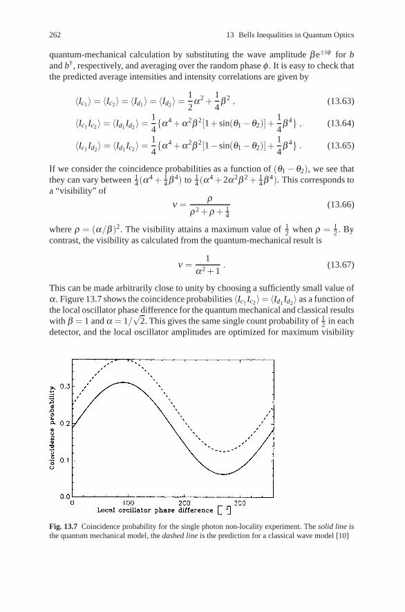
262 13 Bells Inequalities in Quantum Optics
quantum-mechanical calculation by substituting the wave amplitude β e±iφ for band b†, respectively, and averaging over the random phase φ . It is easy to check thatthe predicted average intensities and intensity correlations are given by
〈Ic1〉= 〈Ic2〉= 〈Id1〉= 〈Id2〉=12
α2 +14
β 2 , (13.63)
〈Ic1Ic2〉= 〈Id1Id2〉=14{α4 + α2β 2[1 + sin(θ1−θ2)]+
14
β 4} , (13.64)
〈Ic1Id2〉= 〈Id1Ic2〉=14{α4 + α2β 2[1− sin(θ1−θ2)]+
14
β 4} . (13.65)
If we consider the coincidence probabilities as a function of (θ1− θ2), we see thatthey can vary between 1
4(α4 + 14 β 4) to 1
4 (α4 + 2α2β 2 + 14 β 4). This corresponds to
a “visibility” of
ν =ρ
ρ2 + ρ + 14
(13.66)
where ρ = (α/β )2. The visibility attains a maximum value of 12 when ρ = 1
2 . Bycontrast, the visibility as calculated from the quantum-mechanical result is
ν =1
α2 + 1. (13.67)
This can be made arbitrarily close to unity by choosing a sufficiently small value ofα . Figure 13.7 shows the coincidence probabilities 〈Ic1Ic2〉= 〈Id1Id2〉 as a function ofthe local oscillator phase difference for the quantum mechanical and classical resultswith β = 1 and α = 1/
√2. This gives the same single count probability of 1
2 in eachdetector, and the local oscillator amplitudes are optimized for maximum visibility
Fig. 13.7 Coincidence probability for the single photon non-locality experiment. The solid line isthe quantum mechanical model, the dashed line is the prediction for a classical wave model [10]

13.4 One-Photon Interference 263
Fig. 13.8 Variation of visibility with the amplitude of the local oscillator for the quantum model(solid line) and a classical wave model (dashed line) [10]
in the classical result. However, the quantum mechanical visibility is considerablylarger than that expected classically. This is clearly seen in Fig. 13.8 where thevisibility ν is plotted as a function of the coherent local oscillator amplitude α forthe quantum mechanical single state and the classical wave mode with β = 1.
We thus see that by measuring the coincidence probability in a pair of detectors,it is possible to distinguish between the classical and quantum mechanical models.If the detector efficiencies are less than unity, coincidences will be missed, but thisdoes not affect the measurement of the visibility of the effect.
Preparation of a single photon state may be achieved experimentally by using thesignal beam of a parametric amplifier while monitoring photons in the idler beam[11]. Hong and Mandel [12] described an experiment in which a nearly pure singlephoton state was produced using this method. If the pump for the parametric ampli-fier is derived by frequency doubling a coherent beam, this provides a convenientsource for the local oscillator required in the experiment under discussion.
In order to rigorously rule out classical explanations for the quantum mechanicalresult, it is necessary to show that Bell’s inequality may be violated.
An intensity correlation coefficient is used which involves all four photo-detectors
E(θ1−θ2) =〈(Id1− Ic1)(Id2− Ic2)〉〈(Id1 + Ic1)(Id2 + Ic2)〉
. (13.68)
Evaluating this in terms of the statistics of the input mode u, where ν is the vacuumyields
E(θ1−θ2) =−α2{〈u†u〉sin(θ2−θ1)+ |〈u2〉|sin(θ2 + θ1− ξ )}α4 + 〈u†u〉α2 + 1
4 〈u†2u2〉 (13.69)
264 13 Bells Inequalities in Quantum Optics
where 〈u2〉 = Rexp(iξ ). When a single photon input is considered for u, this re-duces to
E(θ1,θ2) =1
α2 + 1sin(θ1−θ2) . (13.70)
If th coefficient of sin(θ1−θ2) is greater than 1/√
2 it is well-known that this func-tional form for the correlation allows a violation of Bell’s inequalities. This is clearlypossible if α is made sufficiently small. It has been shown [13] that such a violationof Bell’s inequalities is not possible if u is in a coherent state, no matter how smallthe input amplitude may be.
In conclusion, some of the most striking features of non-locality in quantummechanics may be demonstrated using phase-sensitive measurements on the fieldproduced by a single photon. These effects may not be explained classically using aparticle, wave or hidden-variable theory involving local causality.
Exercises
13.1 Derive (13.26) for the correlation function E(θ1, θ2). Show that with thechoice ψ = θ2−θ1 = θ ′1−θ2 = θ ′1−θ ′2 = 1
3(θ1−θ ′2) one obtains (13.27) forB.
13.2 Derive (13.51) for the Bell parameter S for the parametric amplifier .13.3 The state going from the beam splitter in the one-photon interference experi-
ment is the linear superposition state
|ψ〉= 1√2(i|1〉|0〉+ |0〉|1〉) .
Compute the intensity correlations were this state replaced by the mixed state
ρ =12(|1〉u〈1|⊗ |0〉v〈0|+ |0〉u〈0|⊗ |1〉v〈1|)
and show that no violation of the Bell inequality can occur.
References
1. A. Einstein, B. Podolsky, N. Rosen: Phys. Rev. 47, 777 (1935)2. N. Bohr: Phys. Rev. 48, 696 (1935)3. J.S. Bell: Physics 1, 105 (1964); Rev. Mod. Phys. 38, 447 (1966)4. A. Aspect, P. Grangier, G. Roger: Phys. Rev. Lett. 49, 91 (1982). A. Aspect, J. Dalibard,
G. Roger: Phys. Rev. Lett. 49, 1804 (1982)5. M.D. Reid, D.F. Walls: Phys. Rev. A 34, 1260 (1986)6. Z.Y. Ou, L. Mandel: Phys. Rev. Lett. 61, 50 (1988)7. Y.H. Shih, C. Alley: Phys. Rev. Lett. 61, 2921 (1988)

References 265
8. P.G. Kwiat, W.A. Vareka, C.K. Hong, H. Nathel, R.Y. Chiao: Phys. Rev. A 41, 2910 (1990)9. S.M. Tan, D.F. Walls: Optics Commun. 71, 235 (1989)
10. S.M. Tan, D.F. Walls, M.J. Collet: Phys. Rev. Lett. 66, 252 (1991)11. C.A. Holmes, G.J. Milburn, D.F. Walls: Phys. Rev. Lett. A 39, 2493 (1989)12. C.K. Hong, L. Mandel: Phys. Rev. Lett. 56, 58 (1986)13. S.M. Tan, M.J. Holland, D.F. Walls: Opt. Commun. 77, 285 (1990)

Chapter 14Quantum Nondemolition Measurements
Abstract Current attempts to detect gravitational radiation have to take into ac-count the quantum uncertainties in the measurement process. Considering that thedetectors are macroscopic objects in some cases as large as a 10-ton bar, the factthat quantum fluctuations in the detector must be taken into account seems sur-prising. However, as discussed in Chap. 8, gravitational waves interact so weaklywith terrestrial detectors that a displacement of the order of 10−19 cm is expected.To illustrate how the measurement process may introduce uncertainties which ob-scure the signal we consider the simple example of a free mass. A measurementof the position of a free mass with a precision Δxi ≈ 10−19 cm will disturb themomentum by an amount given by the uncertainty principles as Δp ≥ �(2Δxi)−1.The period of the gravitational waves is expected to be about 10−3 s, hence a sec-ond measurement of the position should be made after this time. During this pe-riod, however, the position uncertainty will grow under free evolution by an amountΔx2(τ) = Δx2(0)+ [Δp2(0)τ2/m2]. The following inequality then holds
Δx2(τ)≥ 2Δx(0)Δp(0)τm
. (14.1)
Using the uncertainty principle we then find Δx2(τ) ≥ �τ/m. Taking the detectormass equal to 10 tons, we find Δx ≥ 5× 10⁻¹⁹ cm. That is, the uncertainty intro-duced by the first measurement has made it impossible for a second measurement todetermine with certainty whether a gravitational wave has acted or not. This is thestandard quantum limit.
It is instructive to consider measurements of momentum instead of position. Thefirst measurement of momentum causes an uncertainty in position. This howeverdoes not feed back to disturb the momentum as the momentum is a constant ofmotion for a free mass. Hence, subsequent determination of the momentum maybe made with great predictability. The momentum of a free mass is an example ofa quantum nondemolition (QND) variable. The concept of quantum nondemolitionmeasurements has been introduced over the past few years to allow the detection, inprinciple, of very weak forces below the level of quantum noise in the detector. In thenext section we will give a brief review of the concept of a quantum nondemolitionmeasurement.
267
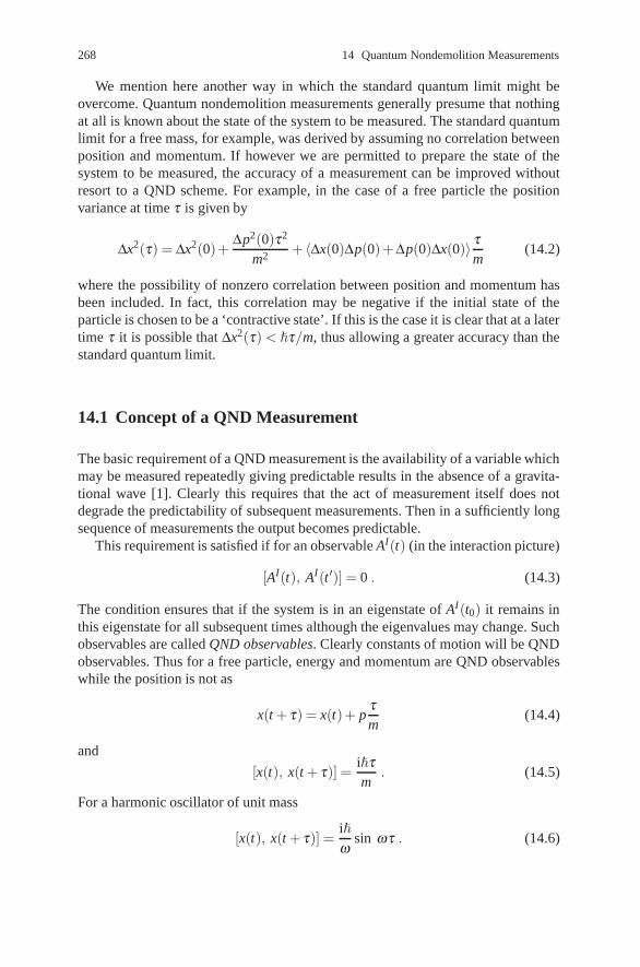
268 14 Quantum Nondemolition Measurements
We mention here another way in which the standard quantum limit might beovercome. Quantum nondemolition measurements generally presume that nothingat all is known about the state of the system to be measured. The standard quantumlimit for a free mass, for example, was derived by assuming no correlation betweenposition and momentum. If however we are permitted to prepare the state of thesystem to be measured, the accuracy of a measurement can be improved withoutresort to a QND scheme. For example, in the case of a free particle the positionvariance at time τ is given by
Δx2(τ) = Δx2(0)+Δp2(0)τ2
m2 + 〈Δx(0)Δp(0)+ Δp(0)Δx(0)〉 τm
(14.2)
where the possibility of nonzero correlation between position and momentum hasbeen included. In fact, this correlation may be negative if the initial state of theparticle is chosen to be a ‘contractive state’. If this is the case it is clear that at a latertime τ it is possible that Δx2(τ) < �τ/m, thus allowing a greater accuracy than thestandard quantum limit.
14.1 Concept of a QND Measurement
The basic requirement of a QND measurement is the availability of a variable whichmay be measured repeatedly giving predictable results in the absence of a gravita-tional wave [1]. Clearly this requires that the act of measurement itself does notdegrade the predictability of subsequent measurements. Then in a sufficiently longsequence of measurements the output becomes predictable.
This requirement is satisfied if for an observable AI(t) (in the interaction picture)
[AI(t), AI(t ′)] = 0 . (14.3)
The condition ensures that if the system is in an eigenstate of AI(t0) it remains inthis eigenstate for all subsequent times although the eigenvalues may change. Suchobservables are called QND observables. Clearly constants of motion will be QNDobservables. Thus for a free particle, energy and momentum are QND observableswhile the position is not as
x(t + τ) = x(t)+ pτm
(14.4)
and
[x(t), x(t + τ)] =i�τm
. (14.5)
For a harmonic oscillator of unit mass
[x(t), x(t + τ)] =i�ω
sin ωτ . (14.6)

14.1 Concept of a QND Measurement 269
and[p(t), p(t + τ)] = i�ω sin ωτ , (14.7)
thus position and momentum are not QND observables for the harmonic oscillator.There are, however, QND observables for the harmonic oscillator. We define the
explicitly time dependent quadrature phase amplitudes for the oscillator as follows.
X1(t) = aeiωt + a†e−iωt (14.8)
andX2(t) =−i(aeiωt −a†e−iωt) . (14.9)
In the Heisenberg picture the quadrature phase operators are given by
X1 = a + a† , (14.10)
X2 =−i(a−a†) , (14.11)
which clearly shows that the quadrature phase operators are constants of the motion.In terms of the position and momentum the quadrature phase operators are
X1(t) =(
2ω�
)1/2
[x(t)cos ωt− p(t)ω
sin ωt] (14.12)
and
X2(t) =(
2ω�
)1/2
[x(t)sin ωt +p(t)ω
cos ωt] . (14.13)
Thus the X1 and X2 axes rotate with respect to the position and momentum axes ofphase space, at frequency ω .
Fig. 14.1 Error box in thephase plane for a harmonicoscillator. The error boxrotates with respect to the xand p/ω axes but is stationarywith to the X1, X2 axes

270 14 Quantum Nondemolition Measurements
The behaviour of X1 and X2 are most easily discussed with reference to an am-plitude and phase diagram. In such a diagram the state of the system is representedby a set of points centred on the mean and contained within an error ellipse deter-mined by the variance of the quadrature phases. Alternatively the error box may beregarded as a contour of the Wigner function. In Fig. 14.1 an error ellipse for theoscillator is shown. The error ellipse is stationary with respect to the X1 and X2 axesbut rotates with respect to the x and p axes. This clearly illustrates how uncertaintiesin momentum feed back into position.
14.2 Back Action Evasion
Having first determined the QND variables of the detector it is necessary to couplethe detector to a readout system or meter. It is essential that the coupling to themeter does not feed back fluctuations into the QND variable of the detector. In orderto avoid this it is sufficient if the QND variable A commutes with the Hamiltoniancoupling the detector and the meter, HDM, that is
[A, HDM] = 0 (14.14)
This is known as the back action evasion criterion.In this chapter we are primarily concerned with QND measurements on optical
systems. This requires a slight change in nomenclature. We will refer to the fieldwith respect to which the QND variable is defined as the ‘signal’ rather than thedetector, and the field upon which measurements are ultimately made as the ‘probe’rather than the meter.
14.3 Criteria for a QND Measurement
We need to clearly define the objectives of a quantum nondemolition measurementin an optical context. These objectives may differ depending on the situation of themeasurement. For example, in a transmission with a series of receivers, the goal maybe to tap information from the signal, without degrading the signal transmitted tothe next receiver. In a system used to measure the magnitude of an external force thegoal of the measurement may be state preparation. That is an initial measurementprepares the system in a known quantum state. The presence of the perturbing forcewill be detected by a subsequent measurement on the system. In order to evaluate themerits of a measurement scheme we shall define a set of criteria which we wouldlike to be satisfied in a good measurement. We begin by considering the generalmeasurement scheme depicted in Fig. 14.2 where an observable Xin of the inputsignal is determined by a measurement of an observable Yout of the output probe.The measurement may be characterised by the following criteria [2]:
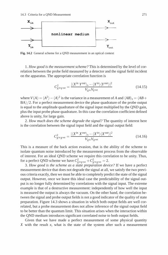
14.3 Criteria for a QND Measurement 271
Fig. 14.2 General scheme for a QND measurement in an optical context
1. How good is the measurement scheme? This is determined by the level of cor-relation between the probe field measured by a detector and the signal field incidenton the apparatus. The appropriate correlation function is
C2X inY out =
|〈X in Y out〉s−〈X in〉〈Y out〉|2VX inVYout
(14.15)
where V (A) = 〈A2〉−〈A〉2 is the variance in a measurement of A and 〈AB〉s = 〈AB+BA〉/2. For a perfect measurement device the phase quadrature of the probe outputis equal to the amplitude quadrature of the signal input multiplied by the QND gain,plus the input probe phase quadrature. In this case the correlation coefficient definedabove is unity, for large gain.
2. How much does the scheme degrade the signal? The quantity of interest hereis the correlation between the signal input field and the signal output field:
C2X inXout =
|〈X in Xout〉s−〈X in〉〈Xout〉|2VX inVXout
(14.16)
This is a measure of the back action evasion, that is the ability of the scheme toisolate quantum noise introduced by the measurement process from the observableof interest. For an ideal QND scheme we require this correlation to be unity. Thus,for a perfect QND scheme we have C2
X inY out +C2X inXout = 2.
3. How good is the scheme as a state preparation device? If we have a perfectmeasurement device that does not degrade the signal at all, we satisfy the two previ-ous criteria exactly, then we must be able to completely predict the state of the signaloutput. However, once we leave this ideal case the predictability of the signal out-put is no longer fully determined by correlations with the signal input. The extremeexample is that of a destructive measurement: independently of how well the inputis measured the output is always the vacuum. On the other hand, the correlation be-tween the signal and probe output fields is not a good indicator of the quality of statepreparation. Figure 14.3 shows a situation in which both output fields are well cor-related, but a probe measurement does not allow inference of the signal output fieldto be better than the quantum limit. This situation arises when the interaction withinthe QND medium introduces significant correlated noise to both output fields.
Given that we have made a perfect measurement of some physical quantityX with the result x, what is the state of the system after such a measurement

272 14 Quantum Nondemolition Measurements
Fig. 14.3 Illustration of asituation in which a value ofthe probe output has beenmeasured, but when mappedonto the error ellipse, doesnot permit an inference ofthe signal to better than thequantum limit
conditioned on the result x? In standard quantum mechanics the conditional stateis generally assumed to be an eigenstate of X with an eigenvalue equal to the mea-sured result, at least for perfect measurements. In the case of the QND measurementscheme above we then expect the state of the signal mode conditioned on the re-sults of the probe measurements should in some limit be an eigenstate of Xout. Ofcourse, the variance of Xout in such a state is zero. Thus as a measure of how wellthe scheme prepares eigenstates at the output we need to consider the conditionalvariance V (Xout|Y out). This quantity is calculated as follows:
The probability to obtain the result Y out for a probe measurement is given by
P(Y out) = Tr{ρout|Y out〉〈Y out|} (14.17)
(assuming perfect readout of the probe state). The conditional state of the signalmode based on this result is
ρout =Trprobe{ρout|Y out〉〈Y out|}
P(Y out). (14.18)
Using this result we see that the conditional distribution for Xout is
P(Xout|Y out) = Trsignal{ρoutsignal|Xout〉〈Xout|}
=P(Xout, Y out)
P(Y out)
where
P(Xout, Y out) = Tr{ρout|Xout〉〈Xout|⊗ |Yout〉〈Y out|} . (14.19)
In many cases of interest P(Xout, Y out) is a bivariate Gaussian. In that case onemay show
V (Xout|Y out) = V (Xout)(1−C2XoutY out) . (14.20)

14.4 The Beam Splitter 273
Thus, the condition for a perfect state reduction in the conditional state is
C2XoutY out = 1 . (14.21)
We shall now analyse some possible measurement schemes and see how well theyapproach the conditions for an ideal measurement.
14.4 The Beam Splitter
We consider first a beam splitter deflecting part of the incident signal field onto a ho-modyne detector, as shown in Fig. 14.4. This will serve as a standard of comparisonfor other measurement schemes. There is obviously little point in constructing com-plicated schemes involving cavities containing nonlinear media if they cannot im-prove on the performance of a beam splitter. We consider the case where the signaland probe fields are single mode with annihilation operators a and b, respectively.The amplitude and phase quadratures of the signal and probe fields are defined as
Xa = a + a† , (14.22)
Xφ =−i(a−a†) , (14.23)
Fig. 14.4 An optical mea-surement scheme for thequadrature phase based on abeam splitter

274 14 Quantum Nondemolition Measurements
Ya = b + b† , (14.24)
Yφ =−i(b + b†) . (14.25)
(This notation assumes that the coherent amplitude of each field is real). Note thataccording to the uncertainty principle
ΔXaΔXφ ≥ 1 (14.26)
where ΔXa and ΔXφ are the square root of the variances. A precise measurementof the amplitude quadrature must therefore be at the expense of uncertainty in thephase. A good back action evading scheme must be able to feed all the quantumnoise induced by the act of measurement into the phase quadrature of the signal.
In the beam splitter the phase change on reflection gives a coupling betweenthe amplitude quadrature of the signal and the phase quadrature of the probe. Weconsider making a measurement on the phase quadrature of the probe in order todetermine the amplitude quadrature of the signal. The input quadrature fields can berelated to the output quadrature fields using the transformation at the beam splitter:
(Xout
aY out
φ
)=
(√1−η2 −ηη
√1−η2
)(X in
aY in
φ
)(14.27)
where η is real and represents the mirror amplitude reflectivity, and there is a π/2phase change upon reflection.
The first criterion for a good QND measurement scheme is that it must be a goodback action evading device. In other words, it must be able to isolate the signal fieldfrom quantum noise introduced by the measurement. How well the beam splitterachieves this is represented by the correlation between the input and the outputsignal fields,
C2X in
a Xouta
=(1−η2)VX in
a
(1−η2)VX ina
+ η2VY inφ
(14.28)
where VX ina
denotes the variance of the signal input, and VY inφ
is the corresponding
variance for the probe. These quantities are a measure of the quantum or classicalnoise present in the input fields at the appropriate qudrature phase. For a beam split-ter with 50% reflectivity, the correlation between the signal input and output is givenby the ratio of the signal noise to the total noise introduced to the system throughboth input ports.
The second criterion reflects how well the scheme acts as a measurement device.The readout measurement is made on the probe output field, so the level of corre-lation between this quantity and the signal field incident on the device determineshow well a measurement can be made. The appropriate correlation function is
C2X in
a Y outφ
=η2 VX in
a
η2 VX ina
+(1−η2)VY inφ
. (14.29)
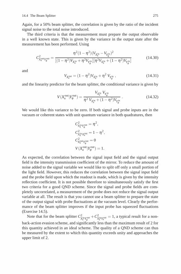
14.4 The Beam Splitter 275
Again, for a 50% beam splitter, the correlation is given by the ratio of the incidentsignal noise to the total noise introduced.
The third criteria is that the measurement must prepare the output observablein a well known state. This is given by the variance in the output state after themeasurement has been performed. Using
C2Xout
a Y outφ
=η2(1−η2)(VX in
a−VY in
φ)2
[(1−η2)VX ina
+ η2VY inφ
][η2VX ina
+(1−η2)VY inφ
](14.30)
andVXout
a= (1−η2)VX in
a+ η2 VY in
φ, (14.31)
and the linearity predictor for the beam splitter, the conditional variance is given by
V (Xouta |Y out
φ ) =VX in
aVY in
φ
η2 VX ina
+(1−η2)VY inφ
. (14.32)
We would like this variance to be zero. If both signal and probe inputs are in thevacuum or coherent states with unit quantum variance in both quadratures, then
C2X in
a Youtφ
= η2,
C2X in
a Xouta
= 1−η2,
C2Xout
a Youtφ
= 0
V (Xouta |Y out
φ ) = 1.
As expected, the correlation between the signal input field and the signal outputfield is the intensity transmission coefficient of the mirror. To reduce the amount ofnoise added to the signal variable we would like to split off only a small portion ofthe light field. However, this reduces the correlation between the signal input fieldand the probe field upon which the readout is made, which is given by the intensityreflection coefficient. It is not possible therefore to simultaneously satisfy the firsttwo criteria for a good QND scheme. Since the signal and probe fields are com-pletely uncorrelated, a measurement of the probe does not reduce the signal outputvariable at all. The result is that you cannot use a beam splitter to prepare the stateof the output signal with probe fluctuations at the vacuum level. Clearly the perfor-mance of the beam splitter improves if the input probe has squeezed fluctuations(Exercise 14.5).
Note that for the beam splitter C2X in
a Y outφ
+C2X in
a Youta
= 1, a typical result for a non-
back-action evasion scheme, and significantly less than the maximum result of 2 forthis quantity achieved in an ideal scheme. The quality of a QND scheme can thusbe measured by the extent to which this quantity exceeds unity and approaches theupper limit of 2.

276 14 Quantum Nondemolition Measurements
14.5 Ideal Quadrature QND Measurements
We now consider another scheme to make perfect QND measurements of thequadrature phase of a single mode field. We shall assume that the amplitude quadra-tures of each mode are coupled. That is, the interaction Hamiltonian has the form
H = �χ Xa Ya (14.33)
where χ is the coupling strength and Xa, Ya are defined by (14.22 and 14.24). ClearlyXa is a QND variable of the signal which satisfies the back action evading condition(14.12). The input and output quadratures are related by
Xouta = X in
a ,
Y outφ = G X in
a +Y inφ ,
where G = χt is known as the QND gain (t being the interaction time).A measurement on the phase quadrature of the probe will be used to determine
the amplitude quadrature of the input signal. To begin we calculate the correlationcoefficients which define the measurement. Clearly CX in
a Xouta
= 1, the signal is com-pletely unaffected by the measurement. The correlation between the input signal andthe phase of the output probe is
CX ina Y out
φ=
G2VX ina
G2VX ina
+VY inφ
(14.34)
where we have taken 〈Y inφ 〉= 0. For a large QND gain G2� 1,
CX ina Y out
φ→ 1 . (14.35)
The conditional variance V (Xouta |Y out
φ ) which determines the value of the scheme asa state preparation device is given by
V (Xouta |Y out
φ ) = VX ina
(1− G2VX in
a
G2VX ina
+VY inφ
)
≈VY in
φ
G2
→ 0 for G2� 1.
Again in the limit of high QND gain this device operates as a good state preparationdevice.
Another measure of the performance of the measurement is the signal-to-noiseratio of the probe output

14.6 Experimental Realisation 277
signalnoise
=〈Y out
φ 〉2VYout
φ
=G2〈X in
a 〉2G2VX in
a+VY in
φ
→ 〈Xina 〉2
VX ina
for G2� 1.
In the limit of large QND gain the signal-to-noise ratio of the output probe is equalto that of the signal input.
14.6 Experimental Realisation
It is possible to achieve a QND coupling of the form in (14.33) by considering twodegenerate modes a and b with frequency ω and orthogonal polarisation, which un-dergo parametric amplification [3]. The two polarisation modes initially undergo amixing interaction using polarisation rotators, after which a mixture of the signaland probe fields will propagate along each of the ordinary and orthogonal extror-dinary axis of a KTP crystal pumped by a pulsed intense classical field. After thisamplification step the fields then pass through a second polarisation rotator adjustedto give the same mixing angle as the first. In order to ensure that the device operatesas an ideal QND scheme the mixing angle of the rotators must be carefully adjusted.The situation is depicted in Fig. 14.5.
The transformation performed by the polarisation rotators is given by
a(θ ) = acosθ + ibsinθ , (14.36)
b(θ ) = bcosθ + iasinθ , (14.37)
with θ being the mixing angle. The transformation in the parametric amplificationprocess is
Fig. 14.5 Schematic representation of a perfect QND scheme based on a parametric interaction

278 14 Quantum Nondemolition Measurements
a(r) = acoshr + ib† sinhr , (14.38)
b(r) = bcoshr + ia† sinhr , (14.39)
where r is related to the parametric gain Gf by Gf = er. Using these transformationsfor the system in Fig. 14.5, we find that the transformations for the signal and probequadratures are
Xouta = X in
a , (14.40)
Xoutφ = X in
φ +(Gf−G−1f )Y in
φ , (14.41)
Y outa = Y in
a − (Gf−G−1f )X in
a , (14.42)
Y outφ = Y in
φ , (14.43)
where we have taken the polarisation mixing angle to be
θ = arc cos
⎛⎝ Gf + 1√
2(G2f + 1)
⎞⎠ . (14.44)
Clearly this represents an ideal QND scheme.In the experiment of La Porta et al. [3], the incident signal was in a coherent state
while the probe was in the vacuum state at input. The measured gain was Gf = 1.33thus giving θ = 8◦. The output quadratures are measured by phase sensitive homo-dyne detection using polarisation beam splitters. To demonstrate that the experimentis operating as a back action evading measurement, three quantities were measured.Firstly the variances of each quadrature of the signal and probe were measured,with the gain both on and off. The probe shows a large noise in only one quadraturewhen the paramp was on. This is a reflection of the gain term appearing in the am-plitude quadrature of the probe. The phase quadrature noise was at the shot-noiselevel. Secondly, the signal variances alone were measured showing a similar effect.Finally the variance of the quantities
X± = (Gf−G−1f )Xout
a ±Youta (14.45)
was measured. For the choosen input states one easily verifies that
V (X+) = 1 , (14.46)
V (X−) = 4(Gf−G−1f )2 . (14.47)
These quantities were measured by adjusting the relative gain of the photo-currentamplifiers to weight the Xout
a quadrature as indicated. This ensures that any correla-tion between Xout
a and Y outa will give maximum cancellation of the noise from each
quadrature seperately in the variances for X±. The results of this experiment are

14.7 A Photon Number QND Scheme 279
Fig. 14.6 The combinationof the amplified signal andprobe quadrature at outputversus the phase of the localoscillator. The variance of X –occurs at integer multiples ofπ. The dotted line correspondsto the case of the paramp off,and is identical to randomlyadded shot-noise levels of thesignal and probe. The noisereduction is 0.6 dB below thecombined shot-noise level.From Arthur La Porta: Phys.Rev. Lett. 62, 28 (1989)
shown in Fig. 14.6. The results of all experiments taken together clearly indicatethat the scheme is operating as a back action evasion device.
Recently, QND experiments have been performed [4] with two-photon transi-tions in three-level atoms, where the signal amplitude is strongly correlated withthe probe phase. The measurement correlation between the signal in and the probeout is C2
X ina Y out
φ= 0.45 and the back action evasion correlation between signal in and
signal out is C2X in
a Y outφ
= 0.9. The overall performance measure of this device as a
QND optical tap is then determined by C2X in
a Y outφ
+C2X in
a Xoutφ
= 1.35, which exceeds
the beam splitter limit of one, but is still well below the optimal value of 2.
14.7 A Photon Number QND Scheme
We turn now to a scheme to measure the photon number in the signal field. Conven-tional photon counting techniques absorb quanta. The scheme considered is a truenondemolition measurement of photons in that no photons are absorbed from thesignal field [5].
Consider the coupled signal/probe system described by the interaction Hamilto-nian
H1 = �χa†ab†b (14.48)
where a refers to the signal mode, and b to the probe. Such a coupling can occurin a four wave mixing process in which case χ is proportional to the third-ordernonlinear susceptibility.
Clearly, a†a is a constant of the motion and is thus a QND variable for the signal.The solution of the Heisenberg equations of motion gives

280 14 Quantum Nondemolition Measurements
a(t) = e−iχb†bta(0) , (14.49)
b(t) = e−iχa†atb(0) . (14.50)
These equations describe a mutual intensity-dependent phase shift for the signaland probe fields. If we can measure this phase shift on the probe, information onthe signal photon number may be obtained. The probe phase shift may, in fact, bedetermined by homodyne detection of a probe quadrature.
Using (14.24 and 14.25) the phase quadrature for the probe field becomes
Y outφ = cos(κa†a) Y in
φ − sin(κa†a) Y ina (14.51)
where κ = χt. It would appear from this equation that the signal operator that weactually measure is not simply a†a but a nonlinear function of a†a. However in anypractical scheme κ is so small that we may approximate the trignometric functionsby the lowest order in κ . Thus, we use
Y outφ = Y in
φ −κa†a Y ina . (14.52)
What quantity plays the role of the QND gain in this scheme? To answer thisquestion we need to evaluate the correlation functions which provide criteria for thequality of the QND measurement. The first of these functions is
C2a†aY out
φ=|〈a†aY out
φ 〉− 〈a†a〉〈Y outφ 〉|2
V (a†a)V (Y outφ )
=κ2〈Y in
a 〉2V (a†a)V (Y in
φ )+ 2κF1 + κ2F2
where
F1 = 〈a†a〉〈Y ina , Y in
φ 〉s ,
F2 = V (a†a)〈Y inφ 〉2 +V(Y in
a )(V (a†a)+ 〈a†a〉2)
and the symmetrised correlation function is defined by
〈A,B〉s =12〈AB + BA〉− 〈A〉〈B〉 . (14.53)
If we now assume 〈Y ina 〉2 � V (Y in
a ), V (Y inφ ) (that is the coherent amplitude of the
probe is much greater than the fluctuations in either quadrature), we find,
C2a†aY out
φ→ 1 (14.54)
when 〈Y ina 〉 is large. It would thus appear that the coherent amplitude of the probe
plays the role of the QND gain. This result is easily understood in terms of a complex
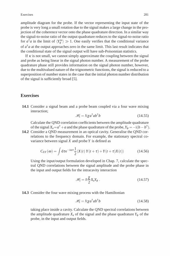
Exercises 281
amplitude diagram for the probe. If the vector representing the input state of theprobe is very long a small rotation due to the signal makes a large change in the pro-jection of the coherence vector onto the phase quadrature direction. In a similar waythe signal-to-noise ratio of the output quadrature reduces to the signal-to-noise ratiofor a†a in the limit of 〈Y in
φ 〉 � 1. One easily verifies that the conditional variance
of a†a at the output approaches zero in the same limit. This last result indicates thatthe conditional state of the signal output will have sub-Poisonnian statistics.
If κ is not small, we cannot simply approximate the coupling between the signaland probe as being linear in the signal photon number. A measurement of the probequadrature phase still provides information on the signal photon number, however,due to the multivalued nature of the trignometric functions, the signal is reduced to asuperposition of number states in the case that the initial photon number distributionof the signal is sufficiently broad [5].
Exercises
14.1 Consider a signal beam and a probe beam coupled via a four wave mixinginteraction;
HI = �χa†ab†b (14.55)
Calculate the QND correlation coefficients between the amplitude quadratureof the signal Xa=a†+a and the phase quadrature of the probe,Yφ =−i(b−b†).
14.2 Consider a QND measurement in an optical cavity. Generalise the QND cor-relations to the frequency domain. For example, the stationary spectral co-variance between signal X and probe Y is defined as
CXY (ω) =∫
dτe−iωτ 12〈X(t) Y (t + τ)+Y(t + τ)X(t)〉 (14.56)
Using the input/output formulation developed in Chap. 7, calculate the spec-tral QND correlations between the signal amplitude and the probe phase inthe input and output fields for the intracavity interaction
HI = �χ2
XaYφ . (14.57)
14.3 Consider the four wave mixing process with the Hamiltonian
HI = �χa†ab†b (14.58)
taking place inside a cavity. Calculate the QND spectral correlations betweenthe amplitude quadrature Xa of the signal and the phase quadrature Yφ of theprobe, in the input and output fields.
282 Quantum Nondemolition Measurements
14.4 Consider a degenerate parametric amplifier inside a resonant two-sided op-tical cavity with mirrors with loss rates γ1,γ2. Treat the left-hand input asthe signal and the right-hand input as the probe. Calculate the QND spectralcorrelations between the phase quadratures of the signal and the probe.
14.5 Calculate the QND correlations for a beam splitter with a squeezed inputprobe.
References
1. C.M. Caves, K.S. Thorne, R.W.P. Drever, V.P. Sandberg, M. Zimmerman: Rev. Mod. Phys. 52,341 (1980)
2. M.J. Holland, M.J. Collett, D.F. Walls, M.D. Levenson: Phys. Rev. A 42, 2995 (1990)3. A. La Porta, R.E. Slusher, B. Yurke: Phys. Rev. Lett. 62, 28 (1989)4. J. Ph. Poizat, P. Grangier: Phys. Rev. Lett. (1992)5. G.J. Milburn, D.F. Walls: Phys. Rev A 28, 2065 (1983)
Chapter 15Quantum Coherence and Measurement Theory
Abstract The feature of quantum mechanics which most distinguishes it from clas-sical mechanics is the coherent superposition of distinct physical states. Many of theless intuitive aspects of the quantum theory can be traced to this feature. Does thesuperposition principle operate on macroscopic scales? The famous Schroedingercat argument highlights problems of interpretation were macroscopic superpositionstates allowed. In this chapter we discuss schemes to produce and detect superpo-sition states in an optical context. We shall show that such states are very fragile inthe presence of dissipation and rapidly collapse to a classical mixture exhibiting nounusual interference features.
The superposition principle is also the source of the “problem of measurement”in quantum mechanics. We do not attempt to present a solution to this problem here.Rather we show how the effect of the environment on superposition states enablesa consistent description of the measurement process to be given and which avoidssome of the problems inherent in previous approaches.
15.1 Quantum Coherence
The well known two slit experiment demonstrates the observational consequencesof the coherent superposition of states, namely the possibility of interference pat-terns. In analogy with the classical theory of wave interference the visibility of theinterference pattern in the probability distributions for various measurements can beused as a measure of quantum coherence. (There is a possibility of confusion herewhich should be cleared up. In the interference of waves we are usually concernedwith the interference of two or more field modes. In this chapter however we areconcerned with the superposition of different states of a single mode.)
The essential point in understanding quantum coherence is the physical distinc-tion between the coherent superposition state
|ψ >= ∑j
c j|φ j > (15.1)
283

284 15 Quantum Coherence and Measurement Theory
and the classical mixture
ρm = ∑j|c j|2 |φ j >< φ j| . (15.2)
The density operator corresponding to the pure state in (15.1) is
ρp = ρm + ∑i�= j
cic∗j |φi >< φ j| (15.3)
How is one to distinguish these states in practice? Let X be the operator correspond-ing to some physical quantity with eigenvalues x. The probability distribution for Xin the state |ψ > is then given by
Pp(x) = Pm(x)+ ∑i�= j
cic∗j < x|φi >< φ j|x > , (15.4)
where Pm(x) is the probability distribution for the state ρm given by
Pm(x) = ∑i|ci|2|< x|φi > |2 = ∑
i|ci|2Pφi(x) (15.5)
Measurements of X will distinguish the states ρm and ρp provided the second termin (15.3) is nonzero. We are thus led to define the quantum coherence with respectto the measurement of X by the coherence function
C (x) = ∑i�= j
cic∗j < x|φi >< φ j|x > . (15.6)
How does one choose an operator X such that the resulting probability distributionwill exhibit interference fringes? Clearly one cannot choose operators which arediagonal in the basis {|φi >} as then the coherence function vanishes. The simplestexample of an operator which distinguishes these states is the projector
P = |ψ >< ψ | , (15.7)
with eigenvalues p ∈ {0,1}. Then
Pp(p) = δ1,p (15.8)
while
Pm(p) ={
∑ j |c j|4 ifp = 11−∑ j |c j|4 ifp = 0
(15.9)
The coherence function is
C (p) = (−1)p(∑j|c j|4−1) (15.10)
In practice however there may be no way to measure the operator P.

15.1 Quantum Coherence 285
In quantum optics one either measures photon number (by photon counting) orquadrature phase (by balanced homodyne detection). As an example consider thesuperposition of two number states
|ψ >=1√2(|n1 > +|n2 >) , (15.11)
and the corresponding mixed state
ρm =12(|n1 >< n1|+ |n2 >< n2|) . (15.12)
A measurement of photon number will not distinguish these states, however as thequadrature phase does not commute with the number operator, quadrature phasemeasurements should distinguish the states.
Define the quadrature operator
Xθ = (ae−iθ + a† eiθ ) (15.13)
with eigenstates |xθ >. Using the result
< xθ |n >= (2π)−1/4(2nn!)−1/2Hn(xθ√
2)e−x2
θ /4−inθ (15.14)
one finds
Pm(xθ ) =12(P(1)(xθ )+ P(2)(xθ )) (15.15)
and
C (xθ ) = (2π)−1/2e−x2θ /2(2n1+n2n1!n2!)−1/2 (15.16)
×Hn1(xθ√
2)Hn2(
xθ√2)cos((n1−n2)θ ) (15.17)
whereP(i)(xθ ) = (2π)−1/2(2nini!)−1Hni(
xθ√2)2e−x2
θ /2 (15.18)
Thus a superposition of number states will exhibit interference fringes for somequadrature phase angle θ . In Fig. 15.1 we plot Pp(xθ ) versus xθ for θ = 0. It issurprising that, depending on whether n1− n2 is even or odd, certain phase anglesdo not give interference. However it is quite clear that the superposition of twonumber states will exhibit phase dependent noise despite the fact that number statesthemselves have phase independent noise.
As a second example consider the superposition of two coherent states (so calledcat states)
|ψ >= N (|α1 > +|α2 >) , (15.19)
where
N =(
2 + e−12 (|α1|2+|α2|2)(eα∗1 α2 + eα1α∗2 )
)−1/2(15.20)

286 15 Quantum Coherence and Measurement Theory
Fig. 15.1 A plot of the prob-ability density for the quadra-ture phase with phase angleat zero for a superpositionof two number states, withn1 = 0,n2 = 5
–6 -4 -2 2 4 6
0.1
0.2
0.3
0.4
0.5 Pp(xθ)
xθ
and
ρm =12(|α1 >< α1|+ |α2 >< α2|) (15.21)
In Chap. 17 we discuss how states of this kind have been produced for the centre ofmass degree of freedom for a harmonically trapped ion. For cat states, measurementsof either quadrature phase or photon number should exhibit interference fringes asneither of the corresponding operators commutes with a coherent state projector.However there is an optimal quadrature phase angle which leads to maximum inter-ference.
In the case of photon number one finds
Pp(n) = N 2(P(1)(n)+ P(2)(n)+C (n)) (15.22)
where
C (n) = (1n!
)exp
(−12
(|α1|2 + |α2|2))
((α1α∗2 )n +(α∗1 α2)n) (15.23)
where
P(i)(n) = (1n!
)|αi|2ne−|αi|2 (15.24)
If we write αi = |αi|eiφ then
C (n) = 2(P(1)(n)P(2)(n))1/2 cos(n(φ1−φ2)) (15.25)
and we see that the degree of interference depends on the phase angle between theamplitudes of the superposed states. For simplicity let us take |α1| = |α2| = |α| .Then
Pp(n) = 2N 2(1n!
)|α|2ne−|α |2(1 + cos(n(φ1−φ2)) . (15.26)
When φ1−φ2 = π , Pp(n) is zero for n odd. Thus a superposition of coherent states πout of phase but of equal amplitude will contain only even photon number, a similarsituation to that of a squeezed vacuum state.
In the case of quadrature phase measurements one finds

15.1 Quantum Coherence 287
P(i)(xθ ) = (2π)−1/2 exp
(−|αi|2 +
xθ2− (xθ −αie−iθ )2
2− (xθ −α∗i eiθ )2
2
)
(15.27)and thus
C (xθ ) = (2π
)1/2ℜexp(−1
2(|α1|2 + |α2|2− x2
θ +(xθ −α1e−iθ )2 +(xθ −α∗2 eiθ )2))
(15.28)To gain some insight into these equations we take |α1|= |α2|= |α| and choose
θ = φ+ = (φ1 + φ2)/2 (15.29)
This phase angle bisects the angle between the two coherent states (see Fig. 15.2).We then have
P(1)(x) = P(2)(x) = (2π)−1/2 exp(−(x−2|α|cosφ−)2/2
)(15.30)
andC (x) = 2P(1)(x)cos(2|α|sin φ−(x−|α|cosφ−)) (15.31)
with φ− = (φ1−φ2)/2 and we have put x = xφ+ . Thus
Pp(x) = 2N 2P(i)(x)(1 + cos(2|α|sin φ−(x−|α|cosφ−)) (15.32)
This is a Gaussian centred at 2|α|cosφ− modulated by an interference envelope (seeFig. 15.3)
This result has a simple geometric interpretation. Referring to Fig. 15.2 we seethat projecting the two coherent states onto the xφ+ axis gives a maximum overlapcentred on the mean value < Xφ+ >= 2|α|cosφ−. We conclude that whenever thecoherent states are projected onto a quadrature such that they overlap exactly, theinterference will be maximal. Conversely we expect that if we project the coherent
Fig. 15.2 Phase space repre-sentation of the superpositionof two coherent states. Thedashed line represents thedirection of the quadraturephase angle which exhibitsmaximum interference

288 15 Quantum Coherence and Measurement Theory
Fig. 15.3 The probabilitydensity for the quadra-ture phase at phase angleθ = φ+ = π/2 for a superpo-sition of two coherent stateswith φ− = π/2 . This is thequadrature direction whichbisects the angle between thetwo superposed coherent am-plitudes, and which exhibitsmaximum interference
-4 -2 2 4
0.2
0.4
0.6
0.8
x
P(x)
states onto a quadrature with θ = φ+±π/2 there will be minimum overlap and thusthe least interference, (see Exercise 15.1).
We now need to consider the effect of dissipation on the interference featuresdiscussed above. With this in mind we write the coherence function in terms of thecomplex valued functions C(x),
C (x) = C(x)+C(x)∗ (15.33)
where for a general superposition state
C (x) = ∑i< j
cic∗j < x|φi >< φ j|x > (15.34)
A convenient measure of the degree of quantum coherence is the quantum visibilitydefined by
V (x) =|C(x)|
(P(1)(x)P(2)(x))1/2(15.35)
In all the cases considered above V (x) is unity for all values of x and the statesconsidered thus have maximum quantum coherence. However when dissipation ispresent this is no longer the case.
15.2 The Effect of Dissipation
In this section we show that quantum coherence associated with superposition statesis extremely fragile in the presence of nonunitary effects such as damping. Sucheffects cause a decay of quantum coherence at a rate which is proportional to aparameter which measures the separation of the superposed states. For macroscopicseparations this decay can be very rapid.
We first consider the effects of dissipation. The master equation for a dampedharmonic oscillator in the interaction picture is

15.2 The Effect of Dissipation 289
dρdt
=γ2(2aρa†−a†aρ−ρa†a) (15.36)
where γ is the damping constant and the reservoir is taken to be at zero temperature.We will solve this equation for an initial superposition of coherent states using thenormally ordered characteristic function,
X(λ ,t) = tr(ρ(t)eλ a†e−λ ∗a) (15.37)
Using (15.36) the equation of motion for X(λ ,t) is
∂X∂ t
=− γ2(λ ∗
∂X∂λ
+ c.c.) (15.38)
where c.c. means complex conjugate. The solution to this equation is
X0(λ e−γt/2,λ ∗e−γt/2) (15.39)
whereX0(λ ,λ ∗) = X(λ ,0) (15.40)
For the initial state given in (15.19), a superposition of coherent states, we find
X0(λ ,λ ∗) = N 22
∑i, j=1
e(λ α∗i −c.c.) < αi|α j > (15.41)
Thus
X(λ ,t) = N 22
∑i, j=1
< αi|α j > exp((λ α∗i − c.c.)e−γt/2
)(15.42)
The corresponding solution for the density operator is
ρ(t) = N 22
∑i, j=1
< αi|α j >(1−e−γt) |αie−γt/2 >< α je
−γt/2| (15.43)
Due to the coefficient with i �= j in this expansion the contribution of the off-diagonalterms to the coherence function will be small. Thus the superposition is reduced toa near mixture of coherent states.
The visibility for any measurement is easily found to be
V (x) = |< α1|α2 > |(1−e−γt) (15.44)
where x = xθ for quadrature phase or x = n for number measurements. For shorttimes this is given approximately by
V (x)≈ exp(− γt2|α1−α2|2) (15.45)

290 15 Quantum Coherence and Measurement Theory
Thus the rate at which coherence decays is proportional to the square of the distancebetween the superposed coherent amplitudes. In the last section we considered thecase α1 = −α2 which gave good interference fringes centered on the origin for theappropriate quadrature. However we now see that such fringes must decay rapidlycausing the quadrature phase statistics to be indistinguishable from a classical mix-ture of coherent states.
This result is not confined to amplitude damping. For example the phase diffusionmodel discussed in Exercise 6.3 for which the master equation is
dρdt
=γ2(2a†aρa†a− (a†a)2ρ−ρ(a†a)2) (15.46)
The solution for the matrix elements in the number basis is
< n|ρ(t)|m >= exp(− γ2
t(n−m)2) < n|ρ(0)|m > (15.47)
If ρ(0) is a superposition of number states |n1 > and |n2 > the visibility of thequadrature phase statistics is given by
V (x) = exp(− γt2
(n1−n2)2) (15.48)
which shows a rapid decay when n1−n2 is large.These examples are special; the visibility in each case decays in the same way
for all measurements which give interference fringes. This is because the superposedstates are eigenstates or near eigenstates of the operator appearing in the irreversiblepart of the evolution equation. This is an important point to which we shall returnin the next section. In other cases the visibility is more complicated. For exampleconsider the effect of phase diffusion on the quadrature phase statistics of a super-position of two coherent states with α1 = −α2 = q0 where q0 is real. If we chooseθ = π/2 (that is we project onto the imaginary axis in the complex amplitude dia-gram) we find that for short times
V (xπ/2)≈ 1− γt(2q0xπ/2)2 (15.49)
As expected the coherence decays from unity at a rate which is proportional to thesquare of the separation of the superposed states. In Fig. 15.4 we plot the probabilitydistribution for quadrature phase at θ = π/2 with a superposition of coherent states,with q0 = 2, subject to phase diffusion with different damping rates.
A similar result may be derived for quadrature phase measurements on a super-position of number states undergoing damping. To show this we use the complexP-representation for the projector |ni >< n j|
|ni >< n j|=∮
c1
dα∮
c2
dβ Pi j(α,β )|α >< β ∗|< β ∗|α >
(15.50)

15.2 The Effect of Dissipation 291
-4 -2 2 4
1
2
3
P(x)
X
(a) (b) P(x)
X -4 -2 2 4
0.4
0.8
1.2
P(x)
X
(c)
-4 -2 2 4
0.4
0.8
1.2
Fig. 15.4 A plot of the probability distribution for quadrature phase, θ = π/2, on an oscillatorprepared in a coherent superposition of coherent states, |2〉+ | − 2〉, which is subject to phasediffusion. (a) γt = 0 (b) γt = 0.1 (c) γt = 0.5. The loss of visibility and spreading of the distributionis a conseqence of phase diffusion
where
Pi j(α,β ) =− 14π2 eαβ (ni!n j!)1/2α−(ni+1)β−(n j+1) (15.51)
and c1,c2 are contours encircling the origin. Thus under time evolution |ni >< n j|evolves to
(|ni >< n j|)t =∮
c1
dα∮
c2
dβ Pi j(α,β ) < β ∗|α >(1−e−γt)
× |αe−γt/2 >< β ∗e−γt/2|< β ∗|α >
(15.52)
Using this result one may show
C(xθ ,t) = (2π)−1/22−(n1+n2)/2(n1!n2!)−1/2(−1)n1+n2
exp
(−x2
θ2− i(n1−n2)θ
)e−γt(n1+n2)/2
min(n1,n2)
∑p=0
2peγt p p!
(n1
p
)(n2
p
)Hn1+n2−2p(
xθ2
) (15.53)
The dominant term in the sum occurs for p = min(n1,n2). For example if n1 > n2
the time dependence of the dominant term is proportional to exp(−γt(n1−n2)/2).As expected the coherence decays at a rate which is proportional to the separationof the states.
15.2.1 Experimental Observation of Coherence Decay
The Haroche group in Paris demonstrated the rapid decay of coherence for a super-position of two coherent states. They used Rydberg atoms in microwave cavities [1].Two Rydberg atomic levels with ground state |g〉 and excited state |e〉 interact with

292 15 Quantum Coherence and Measurement Theory
a cavity field. The cavity field is well detuned from the atomic resonance. The effectof the interaction is to change the phase of the field in the cavity conditional on theatomic state. An effective Hamiltonian for this interaction can be written as
HC = hχa†aσz (15.54)
where σz = |e〉〈e|− |g〉〈g|.If the cavity C is initially prepared in a weak coherent state, |α〉, (in the exper-
iment |α| = 3.1) and the atom is prepared in an equal superposition of the groundand excited states, the total system state evolves to
|ψ(τ) =12
(|g〉|αeiφ 〉+ |e〉|αe−iφ 〉) (15.55)
where φ = χτ , for an interaction time τ . The state in (15.55) is an entangledstate between a two level degree of freedom and an oscillator. To obtain a statewhich entangles the atomic degree of freedom with coherent superpositions of co-herent states we use an independent laser to rotate the atomic states by |g〉 →(|g〉+ |e〉)/√2, |e〉 → (|g〉− |e〉)/√2. The state at the end of this last pulse is
|ψ〉out =12
(|g〉(|αeiφ 〉+ |αe−iφ 〉)+ |e〉(|αeiφ 〉− |αe−iφ 〉)
)(15.56)
If we now measure the atomic state |g〉 (by state selective ionisation in the experi-ment) the conditional state of the field is either
|ψ(g)〉out = N+(|αeiφ 〉+ |αe−iφ〉) (15.57)
or|ψ(e)〉out = N−(|αeiφ 〉− |αe−iφ 〉) (15.58)
where N± is the normalisation constant. These conditional states are superpositionsof coherent states.
In this discussion we ignored the cavity decay as this is small on the time scaleof the interaction time between a single atom and the cavity field. To observe de-coherence we prepare the field in a coherent superposition of coherent states, aspreviously described, and then let it evolve for a time so that there is a significantprobability that at least one photon is lost from the cavity. We then need to find a wayto probe the field state at the end of that time. It was not possible to directly measurethe state of a microwave cavity field directly. Instead the Haroche experiment useda second atom as a probe for the field state.
There are two possible results for the first atomic measurement (g, e) with thecorresponding conditional states given by (15.57 and 15.58). Now consider sendingin another atom after some delay time T and ask (for example) for the probability tofind the second atom in the excited state given one or the other of the two conditionalstates, that is to say, we seek the conditional probabilities p(e|g) and p(e|e) (wherethe conditioning label refers to the result of the first atom measurement). As therespective conditional states are different, these probabilities should be different.The extent of the difference is given by
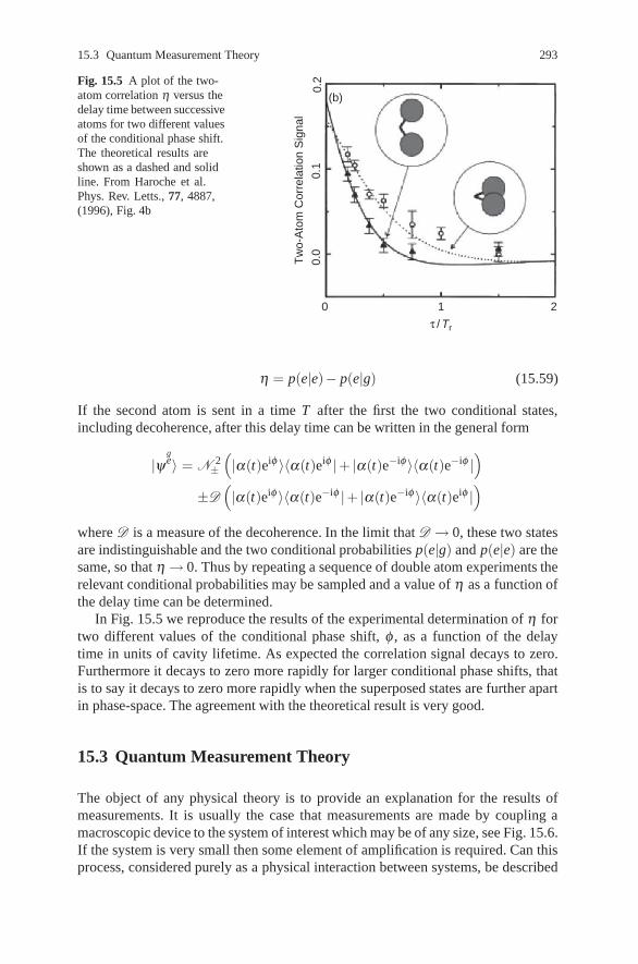
15.3 Quantum Measurement Theory 293
Fig. 15.5 A plot of the two-atom correlation η versus thedelay time between successiveatoms for two different valuesof the conditional phase shift.The theoretical results areshown as a dashed and solidline. From Haroche et al.Phys. Rev. Letts., 77, 4887,(1996), Fig. 4b
0
(b)
0.0
0.1
Tw
o-A
tom
Cor
rela
tion
Sig
nal
0.2
1
τ / Tr
2
η = p(e|e)− p(e|g) (15.59)
If the second atom is sent in a time T after the first the two conditional states,including decoherence, after this delay time can be written in the general form
|ψge〉 = N 2
±(|α(t)eiφ 〉〈α(t)eiφ |+ |α(t)e−iφ〉〈α(t)e−iφ |
)
±D(|α(t)eiφ 〉〈α(t)e−iφ |+ |α(t)e−iφ 〉〈α(t)eiφ |
)
where D is a measure of the decoherence. In the limit that D → 0, these two statesare indistinguishable and the two conditional probabilities p(e|g) and p(e|e) are thesame, so that η → 0. Thus by repeating a sequence of double atom experiments therelevant conditional probabilities may be sampled and a value of η as a function ofthe delay time can be determined.
In Fig. 15.5 we reproduce the results of the experimental determination of η fortwo different values of the conditional phase shift, φ , as a function of the delaytime in units of cavity lifetime. As expected the correlation signal decays to zero.Furthermore it decays to zero more rapidly for larger conditional phase shifts, thatis to say it decays to zero more rapidly when the superposed states are further apartin phase-space. The agreement with the theoretical result is very good.
15.3 Quantum Measurement Theory
The object of any physical theory is to provide an explanation for the results ofmeasurements. It is usually the case that measurements are made by coupling amacroscopic device to the system of interest which may be of any size, see Fig. 15.6.If the system is very small then some element of amplification is required. Can thisprocess, considered purely as a physical interaction between systems, be described
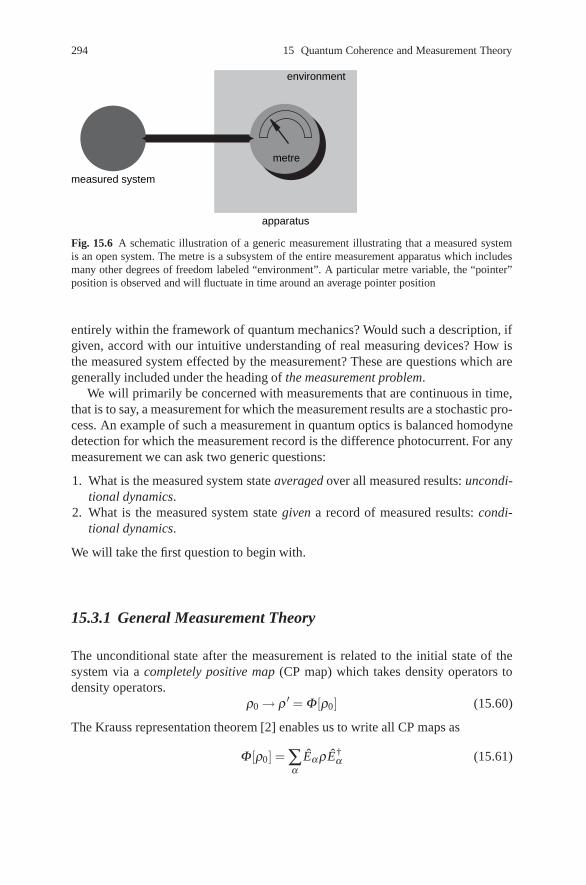
294 15 Quantum Coherence and Measurement Theory
measured system
environment
metre
apparatus
Fig. 15.6 A schematic illustration of a generic measurement illustrating that a measured systemis an open system. The metre is a subsystem of the entire measurement apparatus which includesmany other degrees of freedom labeled “environment”. A particular metre variable, the “pointer”position is observed and will fluctuate in time around an average pointer position
entirely within the framework of quantum mechanics? Would such a description, ifgiven, accord with our intuitive understanding of real measuring devices? How isthe measured system effected by the measurement? These are questions which aregenerally included under the heading of the measurement problem.
We will primarily be concerned with measurements that are continuous in time,that is to say, a measurement for which the measurement results are a stochastic pro-cess. An example of such a measurement in quantum optics is balanced homodynedetection for which the measurement record is the difference photocurrent. For anymeasurement we can ask two generic questions:
1. What is the measured system state averaged over all measured results: uncondi-tional dynamics.
2. What is the measured system state given a record of measured results: condi-tional dynamics.
We will take the first question to begin with.
15.3.1 General Measurement Theory
The unconditional state after the measurement is related to the initial state of thesystem via a completely positive map (CP map) which takes density operators todensity operators.
ρ0→ ρ ′ = Φ[ρ0] (15.60)
The Krauss representation theorem [2] enables us to write all CP maps as
Φ[ρ0] = ∑α
EαρE†α (15.61)

15.3 Quantum Measurement Theory 295
where
∑α
E†α Eα = 1 (15.62)
ensures normalisation. The sum in (15.61) could stand for an integral. The Kraussdecomposition is not unique: there is a unitary equivalence class of possible Kraussdecompositions.
Suppose we measure some metre quantity for which the result is a real number x.The statistics of measurement results is given in terms of a positive operator, F(x)as
P(x) = tr(ρF(x)) (15.63)
which is the most general way to construct probability distributions from densityoperators allowed by the quantum formalism. The conditional state given the mea-surement result is,
ρ (x) =ϒ (x)ρϒ †(x)
P(x)(15.64)
where F(x) = ϒ †(x)ϒ (x). The unconditional state is given by,
ρ ′ =∫
dxP(x)ρ (x) =∫
dxϒ (x)ρϒ †(x) (15.65)
which relates the CP map to the measurement operators.As an example of this formalism we consider the measurement of a generic two
level system (a qubit) coupled to a measurement apparatus for which the pointervariable has real eigenvalues. To specify the nature of the measurement we needonly specify the Krauss measurement operator ϒ (x),
ϒΔ (x) = (2πΔ)−1/4 exp
[− (x−κσz)2
4Δ
](15.66)
where σz = |1〉〈1|− |0〉〈0| is the measured system observable and {|0〉, |1〉} are anorthonormal basis for the two level system. (see Exercise 15.5). The probabilitydensity for measurement result, x(t) at time t;
P(x,t) = tr(ρ(t)ϒ †Δ (x)ϒΔ (x)) (15.67)
The moments of this distribution are related to the quantum moments of the mea-sured system observable by
E (x(t)) = κ〈σz(t)〉E ((Δx(t)))2 = Δ + κ2〈(Δσz(t))2〉
Thus we regard Δ as the noise added to the signal by the apparatus. Using the factthat σ2
z = 1 the measurement operator may be written
ϒΔ (x) =√
P1(x)|1〉〈1|+√
P0(x)|0〉〈0| (15.68)

296 15 Quantum Coherence and Measurement Theory
where
Pα(x) = (2πΔ)−1/2 exp
[− (x +(−1)ακ)2
2Δ
](15.69)
where α = 1,0. The unconditional state, is then given by (15.65) as
ρ ′ = p1|1〉〈1|+ p0|0〉〈0|+ e−κ2/2Δ (|1〉〈0|+ |0〉〈1|) (15.70)
where pα = 〈α|ρ |α〉, and α = 0,1. We can now define the good measurement limitas e−κ2/2Δ << 1, and the measurement result statistics easily enable the eigenstatesof σz to be resolved. In this limit the unconditional post measurement state is diag-onalised in the eigenbasis of σz.
15.3.2 The Pointer Basis
How does the construction of a physical measurement apparatus determine whatsystem quantity is measured? This is one of the key components of the measure-ment problem. To understand why there might be a problem we will consider asimple model of the interaction between a measured system S and a measuring de-vice M. Let us first ignore the macroscopic nature of M and simply treat it as asingle quantum system with one degree of freedom. As we shall see such an as-sumption does not lead to an adequate description of the measurement process. Themacroscopic nature of M is essential for a complete description.
Let {|mi >} denote a set of eigenstates of some meter quantity and let {|si >}denote the eigenstates which diagonalise the system operator we are seeking to mea-sure. Suppose the initial state of the system is |m0 > ⊗|si > , and further supposethat under unitary evolution this state evolves to
|ψi(t) >= |mi >⊗|si > (15.71)
Then for a general system state
|ψ >= ∑i
ci|si >⊗|m0 > (15.72)
the state at time t will be
|ψ(t) >= ∑i
ci|mi >⊗|si > (15.73)
We regard mi as the value read-out from the meter scale. If an observer finds themeter in a state |m j > (with probability |c j|2 ) the system is subsequently (i.e. con-ditionally ) described by the state |s j >. It is clear that in effect we have measuredsome physical quantity S which is diagonal in the basis {|si >} ,

15.3 Quantum Measurement Theory 297
S = ∑i
ai|si >< si| (15.74)
Suppose one only knows that a measurement has taken place but we do not selecta particular result. The state of the system must then be described by the reduceddensity operator obtained by tracing out over the meter states,
ρs = ∑i
|ci|2|si >< si| (15.75)
Thus as a result of the measurement the density operator of the system is diagonal inthe basis which diagonalises the measured operator. Alternatively the basis in whichρs is diagonal determines the system operator which has been measured. This is thestandard description of the measurement process. Unfortunately it is inadequate aswe now explain.
The description given above assumed we read out a meter quantity which is di-agonal in the basis {|mi >}. Suppose however we decide to read out another meterquantity diagonal in the basis {|mi >}. We can then express the meter states |mi >in the alternative basis {|mi >} ,
|mi >= ∑j
< m j|mi > |m j > (15.76)
The state of the combined system after the interaction is then
|ψ(t) > = ∑i
ci|mi >⊗|si >
= ∑j
d j|m j >⊗|r j > (15.77)
whered j|r j >= ∑
ici < m j|mi > |si > (15.78)
Although the system meter coupling has not altered there is now some ambiguity asto what system operator has been measured; is it
S = ∑i
ai|si >< si|
orR = ∑
i
bi|ri >< ri| ? (15.79)
This ambiguity can only be removed if we say that the meter is so constructed thatthe only physical property that we readout is the one which is diagonal in the basis{|mi >}. What is the property of the meter which determines such a preferred orpointer basis?
We can answer this question by admitting that a true measuring device must bemacroscopic and thus contain many degrees of freedom. Thus, in addition to the

298 15 Quantum Coherence and Measurement Theory
read-out variable, we must consider the meter as composed of many other degreesof freedom possibly coupled to the the read-out variable. These other degrees offreedom cannot be determined in any realistic scheme and thus may be treated asa environment. In order to model this situation we now divide the measurementscheme into system+meter+environment. The system and meter are directly coupledand the meter is coupled to the environment, see Fig. 15.6. As Zurek has shown itis the nature of the coupling between the meter and the reservoir which determinesthe pointer basis.
In order that the special correlation between the system and the meter given by(15.73) be preserved in the presence of the coupling to the reservoir, described bysome Hamiltonian HME, we require that the pointer basis {|mi >} be a complete setof eigenstates for a pointer quantity M which commutes with HME. This ensures thatfluctuations from the reservoir do not find there way back to the measured systemquantity S. In many situations it may not be possible to find an operator whichsatisfies this condition exactly. However an approximate pointer basis may exist inas much as the diagonal elements of the density operator in such a basis relax on avery long time scale while the off-diagonal elements decay on a much shorter timescale.
Thus it is the meter-reservoir interaction which determines the pointer observ-able M and thus the corresponding pointer basis appropriate to the measurement.The to-be-measured quantity is only defined in the course of the meter-reservoir in-teraction; a situation consistent with Bohr’s general description of measurement inquantum mechanics.
The meter cannot be observed in a superposition of pointer basis states as itsstate vector is being continually collapsed. It is the monitoring of the meter by thereservoir which results in the apparent state reduction of the system and the meter isso constructed to ensure that this occurs. The correlations between the correspond-ing system and pointer basis states are preserved in the final mixed state densityoperator
∑i, j
cic∗j |mi >< mj|⊗ |si >< s j| →
∑i|bi|2|mi >< mi|⊗ |rp
i >< rpi | (15.80)
where {|rpi >} are the system states determined by the pointer basis, referred to as
the relative states.There is a close connection between the concept of a quantum nondemolition
measurement and the concept of a pointer basis. The condition that an operator Q(t)be a QND variable is that (in the interaction picture)
[Q(t),Q(t ′)] = 0 (15.81)
Applying this idea to the measurement description above it is clear that the pointerobservable P, which determines the pointer basis, must be a QND variable of the
15.5 Model of a Measurement 299
meter. This ensures that an initial eigenstate of P evolves entirely within the pointerbasis set.
In the theory of QND measurements we also require the variable Q to maintainits QND property in the presence of couplings to other systems, the reservoir inour example, which represent further stages of the meter device. This will be trueprovided the back action evasion criterion is satisfied
[Q(t),HME] = 0 (15.82)
where HME represents the interaction Hamiltonian between the system of the QNDvariable and other systems to which it is coupled (the reservoir in our case). Thisproperty is precisely the property that the pointer observable must satisfy. We maythus view the pointer observable as a QND variable of the meter which is coupledto the environment by a back action evasion coupling.
15.4 Examples of Pointer Observables
In Sect. 15.1 we considered a number of models which lead to the density operatorbecoming diagonal in a preferred basis. For example, if the meter is a harmonicoscillator coupled to the bath by
HME = a†aΓE (15.83)
so that it evolves according to the master equation (15.46) the state of the meterbecomes diagonal in the number basis. The pointer observable is a†a and (15.83)represents an ideal back action evasion coupling.
As another example suppose that the amplitude of an oscillator is coupled to theenvironment by
HME = aΓ † + a†Γ (15.84)
This is not a back action evasion coupling, however the meter state tends to becomediagonal in the coherent state basis which are eigenstates of the operator a. Unfor-tunately the diagonal elements of the density operator in this basis are also changed.However as we saw in (15.43) for short times the diagonal elements do not changemuch, yet coherence between states separated by large coherent amplitudes decayquite rapidly. In this case we can say that the coherent states are an approximatepointer basis.
15.5 Model of a Measurement
We are now able to consider a full model of a quantum limited measurement in-cluding the interaction of the meter with the environment. The quantum systemand meter are taken to be harmonic oscillators with annihilation operators a and b

300 15 Quantum Coherence and Measurement Theory
respectively. The coupling between the system and the meter is taken to be quadraticin the system amplitude and the interaction Hamiltonian is
HSM =h2
a†a(bE∗+ b†E) . (15.85)
Such a system may represent a four wave mixing interaction in quantum optics,where one field is taken as classical of amplitude E . The measured system operatoris, as we shall see, a†a (or some function thereof).
We assume that mode b is coupled to the environment by amplitude coupling
HME = bΓ † + b†Γ . (15.86)
This will determine a particular pointer basis. There are good physical reasons whythis is a suitable choice for HME. First, if the oscillators are realised as field modesthis coupling represents the usual system-bath interaction of a linear loss mecha-nism. In particular it could represent the interaction of a field mode with a photo-electron counter. Perhaps the most important reason for choosing HME in this formhowever is that it leads to the coherent state pointer basis. As coherent states havea well defined semiclassical limit this is a desirable basis for a real (i.e. classical)measuring device. We now solve for the complete dynamics of the system and metercoupled to the bath.
The density operator for the system and meter after tracing out the reservoirobeys the master equation
dρdt
=−i2
[(Eb† + E∗b)a†a,ρ ]+γ2(2bρb†−b†bρ−ρb†b) (15.87)
We have assumed the environment is at zero temperature. Initially the state of thesystem is arbitrary while the meter is in the ground state
ρ(0) =∞
∑n,m=0
(ρnm|n >< m|)S⊗ (|0 >< 0|)M (15.88)
where we have expanded the system state in energy eigenstates and ρnm =<n|ρs(0)|m >. Equation (15.87) may be solved by the characteristic function. Thesolution is,
ρ(t) =∞
∑n,m=0
exp
( |E|2γ2 (n−m)2(1− γt/2− e−γt/2)
)
× (|n >< m|)S⊗( |αn(t) >< αm(t)|
< αm(t)|αn(t) >
)M
(15.89)
where |αn(t) > is a meter coherent state with
αn(t) =En
γ(1− e−γt/2) (15.90)

15.5 Model of a Measurement 301
In the long time limit we have
ρ→∑n
P(n)(|n >< n|)S⊗ (|αn >< αn|)M (15.91)
where P(n) is the initial number distribution for the system. This is a mixture ofnumber states in the system, perfectly correlated with a mixture of coherent statesin the meter. It is thus of the general form of (15.80). The coherent states |αn >are the pointer basis states and the number states the corresponding relative states.The amplitude of the coherent states can be made arbitrarily large by increasing thestrength of the system meter coupling E . Hence this model includes amplificationin a natural way. The large E limit is the appropriate limit for an accurate measure-ment [3]. In fact the states |αn > for different values of n become approximatelyorthogonal as the coupling strength is increased.
We have assumed in this analysis that the environment is at zero temperature.For photoelectric detection this is a good assumption at optical frequencies. Werethe environment not taken at zero temperature there would be an additional thermalspread in the diagonal part of the meter states.
This model contains all the features of the measurement process discussed inSect. 15.3.2. The correlations between the system and the meter are created by uni-tary evoultion. The (almost complete) reduction of the meter states to the pointerbasis (the coherent states) occurs as a result of nonunitary dissipative evolution,which causes the off-diagonal elements of the meter state in the pointer basis to de-cay. It is clear that the model represents the measurement of some function of thesystem number operator a†a. To determine what this function is we must reconsiderthe interpretation of the environment as a photoelectron counter. If we assume thatevery meter quanta lost to the environment is actually counted in the detector, a fullanalysis shows that in fact the model describes the measurement of the square of thenumber operator.
From (15.91) we can calculate the reduced state of the system by tracing outover the meter states. The resulting state has an exponential decay of off-diagonalelements in the number basis which goes as t2 for short times. Such a dependenceindicates that for short times a Markovian evolution equation does not describe theevolution of the system state. However if the rate of photon counting, γ , is verylarge then this short time behaviour is rapidly superceeded by an exponential lineardependence. In this case the effective master equation for the system state is
dρS
dt=− |E|
2
2γ[a†a,
[a†a,ρS
]](15.92)
In this strong measurement limit we see that as far as the system is concerned theeffect of the measurement of photon number is to induce a diffusion in the oscillatorphase. In some sense the phase is the conjugate variable to the photon number sothis result is consistent with the uncertainty principle.

302 15 Quantum Coherence and Measurement Theory
15.6 Conditional States and Quantum Trajectories
We turn now to discuss the second question that may be asked of a measured system:what is the conditional state conditioned on a measurement result? In Chap. 6 wediscussed an approach to solving master equations based on unravelling the solutionas an average over a quantum trajectory: a solution to a stochastic master equationor stochastic Schrodinger equation. Here we will show that a quantum trajectory candescribe the conditional evolution of the state of a continuously measured system,conditioned on the stochastic measurement record.
A simple model for continuous can be built out of the two-level mode discussedin Sect. 15.3.1. To get to a continuous measurement we let readouts occur at Poissondistributed times at rate γ . The system then obeys the master equation
ρ = −i[H,ρ ]+ γ(∫ ∞
−∞dxϒΔ (x)ρϒ †
Δ (x)−ρ)
= −i[H,ρ ]− γ4
(1− e−κ2/2Δ
)[σz, [σz,ρ ]]
Clearly this describes a QND measurement of σz. We now take the limit of weak,rapid measurements γ >> 1, Δ >> κ2 to get
ρ =−i[H,ρ ]−D[σz, [σz,ρ ]] (15.93)
where D = γκ2
8Δ is the decoherence rate in the σz basis. When D is large decoherenceis rapid, which should correspond to a good measurement.
The measurement record is a real valued classical stochastic variable, x(ti), con-ditioned on the state of the system. To get a continuous stochastic record we definea stochastic differential: dy(t) = dN(t)x(t) where dN(t) is a Poisson process:
dN(t)2 = dN(t)E (dN(t)) = γdt
We can now take the diffusive limit. Consider a time δ t such that γδ t >> 1 yet,Dδ t << 1.
E (y(t + δ t)− y(t)) ≈ γδ tκ〈σz(t)〉c (15.94)
E ((y(t + δ t)− y(t))2 ≈ γδ tΔ (15.95)
we can then approximate the observed process by the Ito stochastic d.e.
dy(t) = γκ[〈σz(t)〉cdt +(8D)−1/2dW(t)
](15.96)
where dW(t) is the Wiener process: E (dW (t)) = 0, E (dW (t)2) = dt. If D is large,then we will have a good signal-to-noise ratio.

15.6 Conditional States and Quantum Trajectories 303
Under the same assumptions we can derive the conditional master equation andthe stochastic Schrodinger equation for this measurement. Using (15.64 and 15.67)and taking the limit of weak rapid measurement as above we find that the conditionalmaster equation is
dρc(t) =−i[H,ρc(t)]dt−Ddt[σz, [σz,ρc(t)]]+√
2DdW (t)H [σz]ρc(t) (15.97)
and the stochastic Schrodinger equation is
d|ψc(t)〉 = −iHdt|ψc(t)〉−Ddt[1−2〈σz〉cσz + 〈σz〉2
] |ψc(t)〉
+√
2D(σz−〈σz〉c)dW (t)|ψc(t)〉 (15.98)
This leads us to define a quantum limited measurement as measurement for whichthe signal-to-noise is determined only by the intrinsic quantum noise of the mea-sured system, and the minimum back-action noise consistent with the uncertaintyprinciple. Under these conditions the decoherence rate is determined only by theback-action noise due to measurement. The example considered here is an exampleof a quantum limited measurement. Usually a measurement is not quantum-limitedas the system dynamics has other irreversible channels (e.g. dissipation) and othersources of noise (e.g. thermal) are added to the measured signal.
The stochastic master equation has an interesting property. Using (15.97) we canderive equations of motion for the conditional mean value of σz. Define zc = 〈σz〉c
dzc = (. . .)dt + 2√
D(1− z2c)dW (t) (15.99)
where . . . refers to that part of the dynamics arising directly from the Hamiltonianterm. If we assume that [σz,H] = 0, the stochastic dynamics is determined entirelyby the measurement. It is then clear that there are two fixed points, zc = ±1 whichcorrespond to two eigenstates of σz. In a simulation the result is that the condi-tional state tends to localise on one or the other of the eigenstates of σz. This is thecontinuous measurement version of quantum state reduction.
15.6.1 Homodyne Measurement of a Cavity Field
Consider now a single mode cavity damped into a zero temperature heat bath (seeSect. 6.1). The environment is the multi-mode field external to the cavity. Someof these external modes are coupled into a balanced homodyne detection system.The change in the state of the system, over a time interval dt, can be described bya single jump operator a. In what follows we choose the units of time so that thecavity decay constant, γ is unity. We can define two Krauss operators. Firstly wedefine Ω1 = a
√dt, corresponding to a conditional Poisson process with probability
〈a†a〉dt. Normalization requires a second Krauss operator, Ω0 = I−a†adt/2− iHdt,

304 15 Quantum Coherence and Measurement Theory
where H is Hermitian. Then the unconditional master equation without feedback isjust the familiar Lindblad form
dρ = Ω0ρΩ0 + Ω1ρΩ1−ρ
= −i[H,ρ ]dt + aρa†dt− 12(a†aρ + ρa†a)dt
≡ −i[H,ρ ]dt +D [a]ρdt . (15.100)
A fermionic example is given in [4].In homodyne detection, the output field from the cavity is mixed with a strong
coherent field, the local oscillator. This corresponds to a displacement of the cavityfield a. Obviously this does not change the unconditional dynamics of the cavityfield. With this in mind we first note that given some complex number α = |α|eiφ ,we may make the transformation
a→ a + α
H → H− i|α|2
(e−iφ a− eiφa†) (15.101)
and obtain the same master equation. In the limit as |α| becomes very large, the rateof the Poisson process is dominated by the term |α|2. In this case it may becomeimpossible to monitor every jump process, and a better strategy is to approximatethe Poisson stochastic process by a Gaussian white-noise process.
For large α , we can consider the system for a time δ t in which the system changesnegligibly but the number of detections δN(t) ≈ |α|2δ t is very large; then we canapproximate δN(t) as
δN(t)≈ |α|2δ t + |α|〈e−iφ a + a†eiφ 〉cδ t + |α|δW (t), (15.102)
where δW (t) is normally distributed with mean zero and variance δ t (a Wienerincrement).
We now define the stochastic measurement record as the current
Ihomc (t) = lim
α→∞
δN(t)−|α|2δ t|α|δ t
(15.103)
= 〈e−iφ a + eiφa†〉+ dW(t)/dt . (15.104)
In balanced homodyne detection, this current corresponds to the photo-current.Given this stochastic measurement record, we can determine the conditional stateof the quantum system by the stochastic master equation (SME)
dρa(t) = −i [H, ρc(t)]dt +D [e−iφ a]ρc(t)dt
+H [e−iφ a]ρc(t)dW (t). (15.105)
In the above equations, the expectation 〈a〉c denotes the average over the conditionalstate, Tr(ρca) and H is a superoperator defined in Sect. 6.7

Exercises 305
H [c]ρ = cρ + ρc†−ρ Tr[cρ + ρc†] . (15.106)
Let us define the quadrature phase operator
Xθ = e−iφ a + eiφa† (15.107)
The corresponding stochastic Schrodinger equation is
d|ψc(t)〉 ={−iHdt− 1
2
[a†a−2〈Xθ/2〉c + 〈Xθ/2〉2c
]dt
+ [a−〈X/2〉c]dW (t)}|ψc(t)〉 (15.108)
Note that as |ψc(t)〉 approaches a coherent state for which a|ψc(t)〉= 〈X/2〉c|ψc(t)〉the noise term tends to zero. This leads to the stochastic localisation of the condi-tional state on the set of coherent states. If we ignore normalisation of the state, weget a very direct sense of how the measured photo current conditions the state,
d|ψc(t)〉= dt
[−iH− 1
2a†a + Ihom
c (t)]|ψc(t)〉 (15.109)
Exercises
15.1 Consider the superposition of two coherent states
|ψ >= N (|α0 > +|−α0 >)
where α0 is real. Show that the probability distribution for X1 = a + a† is adouble peaked Gaussian (α0 > 1) while the distribution for X2 =−i(a−a†)shows interference fringes.
15.2 Consider the Hamiltonian
H = hωa†a + hχ(a†a)2 (15.110)
Show that this Hamiltonian can generate a superposition of two coherent statesor two squeezed states of the type discussed in the preceeding questions.
15.3 The spin coherent states are defined by
| j;γ >= exp
(−θ
2(J+e−iφ − J−eiφ )
)| j, j > (15.111)
where γ = eiφ tan θ2 and | j, j > is a Jz eigenstate with eigenvalue j . Consider
the superposition state
|ψ >= N (| j;γ0 > +| j;−γ0 >) (15.112)
306 15 Quantum Coherence and Measurement Theory
with γ0 real. Calculate the probability distributions for Jx,Jy,Jz and show thatthe Jy distribution exhibits interference effects. Give a geometrical interpreta-tion of this result.
15.4 Consider the two mode squeezed vacuum state
|ψ >= (cosh r)−1∞
∑n=0
(tanh r)n |n >1 ⊗|n >2 (15.113)
and the mixed state with the same diagonal distribution
ρ = (cosh r)−2∞
∑n=0
(tanh r)2n|n >1< n|⊗ |n >2< n| (15.114)
Show that these states may be distinguished by the probability distributionsfor the two mode quadrature phase operators X± = a±+ a†
± where
a± =1√2(a1±a2) . (15.115)
15.5 Consider a two-level system with basis states {|0〉, |1〉} coupled impulsivelyto the momentum of a free particle via the Hamiltonian
HI(t) = κ pσzδ (t− tr) (15.116)
with σz = |1〉〈1|−|0〉〈0|. Just prior to the readout at time tr the state of the par-ticle is a Gaussian with the wave function ψ(p) = (2πΔ)−1/4 exp[−x2/(4Δ)].Immediately after the coupling at time tr the position of the particle is mea-sured with perfect accuracy and projected onto the position eigenstate |xr〉.Show that the conditional state of the two level system immediately after thereadout is given by (15.70) with x = xr.
15.6 Show that the measurement operator
ϒΔ (x) = (2πΔ)−1/4 exp
[− (x−κσz)2
4Δ
](15.117)
reduces to a projection operator in the limit σ → 0.
References
1. M. Brune, E. Hagley, J. Dryer, X. Maitre, A. Maali, C. Wunderlich, J.M. Raimond S. Haroche:Observing the Progressive Decoherence of the ‘Meter’ in a Quantum Measurement, Phys. Rev.Letts. 77, 4887 (1996)
2. K. Krauss: States, Effects and Operations: Fundamental Notions of Quantum Theory(Springer-Verlag, Berlin 1983)
3. D.F. Walls, M.J. Collett and G.J. Milburn: Phys. Rev. D 32, 3208 (1985)4. G.J. Milburn, H.B. Sun: Phys. Rev. B 59, 10748 (1999)

Chapter 16Quantum Information
16.1 Introduction
Quantum information theory is the study of communication and information pro-cessing tasks using physical systems that obey the rules of quantum theory. Informa-tion theory was largely the creation of Claude Shannon working at Bell laboratoriesover 50 years ago. Shannon produced an elegant mathematical theory for informa-tion encoding, transmission and decoding in the presence of noise. The work wasgrounded in a deep intuitive knowledge of the nature of noise in classical electron-ics and electromagnetism although it made little reference to the physical carrierof the information or the physical source of the noise. In the early 1980s a numberof pioneers, including Feynman, Fredkin, Bennett, Landauer and Deutsch, began tore-consider these issues in the light of quantum noise. We now know that quantummechanics provides powerful new ways to communicate and process informationthat are impossible, or difficult, in a classical world. Many of these new ideas havehad an impact on quantum optics and some of the first experiments in this burgeon-ing field involve quantum optical systems. In this chapter we will consider someof these developments including quantum cryptography, quantum teleportation andquantum computation.
In classical information theory, the elementary unit of communication and infor-mation processing is the binary digit, or bit, which can take the mutually exclusivevalues 0 or 1. All communication and information processing can be reduced tooperations on strings of binary digits. In 1946 Shannon [1] established a numberof theorems for such operations and founded the subject of information theory [2].Somewhat paradoxically, the key for this development lay in asking how much in-formation is gained when the result of a random binary choice is known. Consider,for example, a fair coin toss. If we code a head as 1 and a tail as 0, it is clear that torecord the result of a single coin toss we require one binary digit. When the resultis known we have gained one bit of information. If we toss N coins there are 2N
possible outcomes, yet to record a single outcome requires only N bits. It wouldappear from this that an intuitive definition for a numerical measure of information
307

308 16 Quantum Information
is the logarithm of the number of possible alternative ways a given outcome can berealised. If all outcomes are equally likely, as in the case of a fair coin toss of Ncoins, the probability of each outcome is 2−N . The information content of a the ithoutcome is then H = − log2 pi where pi = 2−N is the probability of the outcome.The dependence of the information measure on the logarithm of the probability en-sures that information is additive as our intuition with coin tosses would suggest.In general all outcomes are not equally likely. In that case we are led to define theaverage information of an outcome as H =−∑i pi log2 pi. We choose to define ourlogarithms base two as this leads to a measure of information in bits, which appearsmore natural in this context.
16.1.1 The Qubit
Quantum mechanics indicates that, at its most fundamental level, the physical worldis irreducibly random. Given complete knowledge of the state of a physical system(that is a pure state) there is at least one measurement the results of which are com-pletely random. The simplest example is provided by a two-state system such as aspin-half particle, a polarised photon, or a two-level atom. An elementary opticaltwo-state system is a beam splitter, shown in Fig. 16.1. A single photon directedtowards a 50/50 beam splitter will be reflected or transmitted with equal probability(we assume an ideal device that does not absorb the photon). If we place a perfectphoton detector in both output ports of the beam splitter we will get a count at one orthe other detector with equal probability. At first sight it would appear that a singletwo-state system such as this is a perfect quantum coin toss, but the reality is moresubtle.
To understand why this is so consider the example depicted in Fig. 16.2 in whichwe try to toss the quantum coin twice in succession by redirecting the photon to-wards another identical beam splitter. In a real coin toss the outcome is no less
Fig. 16.1 A single photonat a 50/50 beam splitter canbe reflected or transmittedwith equal probability. Aperfect photon detector inboth output ports of the beamsplitter, labeled U (upper) orL (lower), will register a countat one or the other detectorwith equal probability
input light
U-detector
L-detector

16.1 Introduction 309
Fig. 16.2 Tossing a quantumcoin twice. After the firstbeam splitter in Fig. 16.1, asingle photon is redirected,using perfectly reflectingmirrors, towards an identi-cal beam splitter. The deviceis now a Mach–Zehnderinterferometer and can beadjusted, by moving a mirroras indicated, so that the pho-ton emerges with certaintyin the upper output mode.The adjustment can be madeby small displacements onone of the perfectly reflectingmirrors
input light
U-detector
L-detector
uncertain than the first coin toss. Such is not the case for this “quantum coin toss”.In Fig. 16.2 we illustrate a possible way to make the photon choose twice in suc-cession whether to be reflected or transmitted, and immediately recognise the formof a Mach–Zehnder interferometer. Clearly we can set up this device so that thephoton will be detected with certainty in say the upper photon detector. This is verydifferent from tossing two coins in succession.
The explanation of this phenomenon takes us to the heart of why quantum infor-mation theory will necessarily be different from classical information theory. Imme-diately after the first beam splitter the photon is in a quantum superposition of twodistinct spatial modes of the field;
|ψ〉= 1√2(|1〉U ⊗|0〉L + |0〉U ⊗|1〉L) (16.1)
where we have labelled the two output modes as up (U) or lower (L). If we place aphoton detector in both output modes it is easy to see that we will count a photon ineach mode with equal probability. However the state is not a truly random state. Infact it is a pure state, the entropy of which is zero. The beam-splitter has unitarilytransformed the initial pure state |0〉U⊗|1〉L. If the system is caused to pass throughanother beam splitter a further unitary transformation takes place which, for appro-priate path lengths, will produce the state |1〉U ⊗ |0〉L at the output and the photonwill be detected with certainty in the upper detector.
We need to distinguish a true coin toss from a “quantum” coin toss. The key dis-tinguishing feature is the ability of the quantum system to be prepared in a coherentsuperposition of the two mutually exclusive alternatives. This is not possible for aclassical coin toss which is either heads or tails but not both. While it is true that theresult of an arbitrary measurement on a single two state system will give one bit ofinformation in general, the system state is not like a classical coin toss, as the sin-gle photon example illustrates. To distinguish a true one bit classical system from aquantum one bit system we will refer to the quantum case as a qubit. A qubit is then

310 16 Quantum Information
a quantum system which can yield at most one bit of information upon measure-ment, but which can be in a coherent quantum superposition of the two mutuallyexclusive outcomes prior to measurement. In the case of N qubits the system canexist in a superposition of all 2N possible product states of each individual qubit. Itis this exponential rise in the number of states accessible to an N qubit system thatgives quantum information processing its power. We discuss below an example ofhow even a single qubit can be harnessed to do things that a classical one bit systemnever could; secure key distribution.
16.1.2 Entanglement
The key feature of quantum mechanics that lies behind quantum information theoryis quantum entanglement. Quantum entanglement refers to correlations between theresults of measurements made on distinct subsystems of a composite system thatcannot be explained in terms of standard statistical correlations between classicalproperties inherent in each subsystem. An example is provided by the violation ofthe Bell inequality for two distinct two-state quantum systems (see Chap. 13). Ifthe subsystems are time like separated, quantum entanglement implies non-locality.Non-locality means that measurements on distinct subsystems, local measurements,are incapable of determining the joint state of the composite system. While quantumentanglement and non-locality are related they are not the same. It is possible to havenon-locality without entanglement [3].
In quantum optics the simplest source of entanglement is provided by the non-degenerate squeezed vacuum state produced by spontaneous parametric down con-version (see Sect. 5.2.1),
|E 〉= (1−λ2)1/2∞
∑n=0
λn|n〉a⊗|n〉b (16.2)
where λ = tanhr with r the squeezing parameter. Note that this state is a zero eigen-state of the photon number difference operator, na− nb, between the two modes.The entanglement here results from a superposition of the infinite number of in-distinguishable ways we can distribute equal numbers of photons in each mode.The reduced state of each subsystem (modes a and b) is in fact a thermal state(see Sect. 5.2.5). This is the maximum entropy state for a mode with a fixed av-erage energy. Thus while the total state is a pure state with zero entropy, the stateof each subsystem is as uncertain as it can be given the constraint on the averageenergy.
Measurements on the component sub-systems of entangled states are insufficientto completely determine the joint state of the system. In some cases local measure-ments may give no information at all about the joint state and the entropy of thesubsystem reduced states are maximal. Such states are called maximally entangled.

16.1 Introduction 311
An example is provided by the following eigenstates of total photon number,
|ψN〉=1√
N + 1
N
∑n=0
|n〉a⊗|N−n〉b (16.3)
Local measurements on either mode, say a, are described by the reduced densityoperator
ρa = Trb(ρ) (16.4)
where Trb refers to the partial trace over mode b. In this case the resulting reduceddensity operator for each mode is the identity matrix in N + 1 dimensions. Theentropy of such a state is
Sa,b =−Trρa,b lnρa,b = ln(N + 1) (16.5)
which, given the constraint on total photon number, is maximal. In general the en-tropy of each subsystem satisfy an important inequality, the Araki–Lieb inequality,
|Sa−Sb| ≤ S ≤ Sa + Sb (16.6)
where S is the entropy of the state of the joint system. In the case of a pure entangledstate this implies that Sa = Sb.
Entangled states do not necessarily need to be pure states. Furthermore therecan be non-entangled states that still exhibit classical correlations between the sub-systems. If an entangled state interacts with an environment entanglement can bereduced to zero while classical correlations remain. An example is provided by atwo-mode squeezed vacuum state undergoing phase diffusion in each mode. Thesteady state density operator describing such a system is
ρ = (1−λ2)∞
∑n=0
λ2n|n〉a〈n|⊗ |n〉b〈n| (16.7)
which still retains a perfect classical correlation between the photon numbers ineach mode. However as the state is a convex sum of states which factorise, the statein (16.7) is not entangled and in fact is defined as separable.
It seems reasonable to suggest that between pure entangled states and totally sep-arable mixed states there is a gradation of entanglement. To quantify this we requirea measure of entanglement, and a number of such measures for finite dimensionalHilbert spaces have been proposed [4]. The situation for infinite dimensional Hilbertspaces, which is the case for much of quantum optics, is complicated except for aspecial class of states known as Gaussian states. Such states have a Gaussian Wignerfunction. The two mode squeezed state is an example (see Sect. 5.2.4). Further dis-cussion on mixed Gaussian entangled states is given in [5]
When a pure state, |ψ〉 interacts with an environment it undergoes decoher-ence (see Chap. 15) and generally becomes a mixed state, ρ. We can then askfor the probability of finding the initial state, ψ in the ensemble represented by ρ.

312 16 Quantum Information
This probability is given byF = Tr(ρ|ψ〉〈ψ|) (16.8)
which is called the fidelity. Fidelity has a deeper significance in terms of the statis-tical distinguishability of quantum states [6].
16.2 Quantum Key Distribution
For millennia, communicating parties have devised schemes whereby messages canbe authenticated (the signature) and secured from unauthorised access (cryptogra-phy). Modern methods (symmetrical crypto-systems) for secure electronic commu-nication involve the prior exchange of a random number which is called the key. Ifthe communicating parties share this number with each other and no one else, mes-sages can be securely encrypted and decoded. The method however is vulnerableto a third party acquiring access to the key. In this section we will describe howquantum mechanics enables two communicating parties to arrive at a shared securekey via Quantum Key Distribution (QKD).
The idea that quantum mechanics might enable more secure communication washinted at in the work of Wiesner [7] and made explicit in the pioneering work ofBennett and Brassard [8], in which the first QKD protocol, BB84, was presented. Ituses a set of four qubit states to encode one bit. The first experimental demonstra-tion of QKD was made by Bennett, Brassard and co-workers in 1989 [9]. The firstpractical implementation over a kilometer of optical fibre was achieved by Gisin’sgroup in Geneva [10]. The idea has since been elaborated by a number of authorsincluding Ekert [11] who in 1991 showed that EPR entangled states of pairs of pho-tons could also be used for QKD. However here we will describe the minimal QKDscheme of Bennettt, B92 [12], as this scheme is simpler than BB84 (it uses only twonon orthogonal states) and has been successfully implemented in optical fibres overlong distances and in free space communication. In practice however a two stateQKD scheme is not desirable as it is possible to distinguish two non orthogonalstates provided we accept inconclusive outcomes in some trials.
The key idea behind QKD is the Heisenberg uncertainty principle which ensuresthat any attempt to measure a quantum state will change it, and thus eavesdroppingcan in principle be detected. This is related to a powerful theorem in quantum in-formation theory, the “no-cloning” theorem: an unknown quantum state cannot beduplicated [13]. Thus experimental QKD offers important new insights into the na-ture of quantum physics. Let us now follow a classical protocol to establish a sharedrandom key between two communicating parties, called Alice (A) and Bob (B).
Alice and Bob are assumed to have a means to generate completely random bi-nary numbers. Alice generates a random binary number and sends it to Bob, andBob generates a random binary number and compares it to the binary number re-ceived from Alice. If it is the same he tells Alice publicly that this is the case,but does not reveal what the value actually was. If it was the same, Alice and Bob

16.2 Quantum Key Distribution 313
keep this binary number, otherwise they discard it. Alice and Bob then repeat theprocedure for another binary number and continue in this way until they share abinary string that is a subset of the total binary string that Alice sent to Bob. If forsome reason Alice’s binary number fails to get to Bob in a particular run, it makesno difference to the final shared binary string (although it does reduce the rate ofcommunication for the shared binary string). The big problem with this method isthat classically it is possible for an eavesdropper, Eve, to copy Alice’s transmittedbinary number without disturbing it. Then Eve can listen to the public channel andhear Bob telling Alice that this number was the same as his binary number. QKDavoids this problem by making it impossible for Eve to measure (or copy) an un-known quantum state without also disturbing it in general. If Alice and Bob chosecarefully the quantum state encoding their binary numbers an eavesdropper can bedetected by Alice and Bob.
Alice and Bob will communicate with polarised single photon pulses (see Sect.16.4.2 for further discussion). They first need to agree on how to physically im-plement the encoding. Suppose Alice decides to transmit only vertically (V) and+45o (+D) photons. She will send a V-photon when a previously generated ran-dom binary number is a 0 and a +D-photon when the random binary number is a 1.
A : V ↔ 0; +D↔ 1 . (16.9)
Bob and Alice also agree that Bob can make a polarisation measurements of Alice’sphoton in only two directions; horizontally (H) or at −45o (−D). These measure-ments project onto non-orthogonal polarisation states. Bob randomly decides whichof his two allowed measurements he will make on any photon he receives fromAlice. The choice of measurement is made by referring to a previously generatedrandom bit according to the code,
B : 0↔−D; 1↔ H . (16.10)
When Bob measures the polarisation he records the result as a yes (Y) or a no (N)depending on whether the photon was indeed found to have that particular polarisa-tion. Bob will never record a Y if his bit is different from Alice’s (crossed polarisers),and he records a Y on 50% of runs in which their bits are the same. Thus Bob canonly get a Y if his bit is the same as Alice’s (although he may get a N in that caseas well). Finally Bob sends a copy of his results to Alice, over a public channel, buthe does not tell Alice what measurement he made on each bit. Now Alice and Bobretain only those bits for which Bob’s result was “Y”. These bits are the shared key.
If Eve, an eavesdropper, makes a QND polarisation measurement of Alice’stransmitted photons in an attempt to learn what was sent, she will introduce a 25%error rate between Alice and Bob’s shared key. This occurs because her measure-ment will project the transmitted state into the eigenstates corresponding to hermeasurement result and this state may be different from that sent by Alice. Aliceand Bob can test for eavesdropping by agreeing to sacrifice part of their sharedkey to check the error rate. If the error rate is 25% or higher they will suspect an

314 16 Quantum Information
eavesdropper and discard the entire shared key. In reality errors are inevitable, andAlice and Bob will need to agree on an acceptable error threshold less than 25%.
This protocol has been demonstrated experimentally by the group of Hughesat Los Alamos National Laboratory. The requirement that we use single photonstates to code the bits of information places considerable demands on the physicalresources required to implement B92. A considerable effort is being expended torealise single photon pulsed sources. Given such a source we also need to be able toreliably detect single photons, with a small dark count rate, and we need to propa-gate single photon pulses over possibly large distances with as little loss as possible.If the loss rate is too high very few counts will be available to Alice and Bob toconstruct their shared key and thus the data transmission rate could be unaccept-ably low. Finally, if we are to use standard optical fibres to transmit the photons,polarisation encoding is difficult owing to the birefringence of optical fibres.
To overcome this last problem the Los Alamos experiment used an interferomet-ric implementation of B92 [14]. We can use any two state system to represent a qubitand thus any two state system can in principle be used for QKD. An example is pro-vided by a single photon Mach-Zhender (M-Z) interferometer, see Fig. 16.3. TheM-Z interferometer couples two input modes to two output modes, labelled U (forupper) and L (for lower) in Fig. 16.3. The device provides two possible paths for asingle photon input at say U to be transmitted to the output. If path lengths are equalwe can set up the device so that a photon input at U will be counted with certainty atthe L-detector. However we also have the freedom to insert phase shift devices intoeither path and thus change the interference conditions. In particular Alice can inserta phase shift φA into one end of the device co-located with her transmission while
L
single photon pulse
ALICE BOB
ΦB
ΦA
U
L
U
Fig. 16.3 A method to use phase shift coding for coherent pulses in a QKD protocol

16.2 Quantum Key Distribution 315
Bob can insert another phase shift φB co-located with his reception. Let us assumeAlice injects photons into the U input mode and that Bob counts photons only fromthe L detector mode. The input state is |1〉U |0〉L. The beam splitters implement thestate transformations,
|1〉U |0〉L → 1√2(|1〉U |0〉L + |0〉U |1〉L) (16.11)
|0〉U |1〉L → 1√2(|0〉U |1〉L−|1〉U |0〉L) (16.12)
The output state is thus given by
|Ψ〉out =12
(eiφB − eiφA
)|1〉U |0〉L +
12
(eiφB + eiφA
)|0〉U |1〉L (16.13)
The probability that a photon injected by Alice is detected by Bob is then
PD = cos2(
φA−φB
2
)(16.14)
Now if Alice and Bob use phase angles (φA,φB) = (0,3π/2) to encode 0 and(φA,φB) = (π/2,π) to encode 1, they have an exact realisation of B92, where po-lariser angels are replaced by path length differences.
To realise a M-Z interferometer using optical fibres for each of the paths is diffi-cult if the arms extend over large distances. Small fluctuations in phase shifts alongeach path would lead to a very unstable interferometer. In the Los Alamos experi-ment this problem was overcome using a single optical fibre for both arms with aunbalanced M-Z interferometer (a Franson-type interferometer) at either end, seeFig. 16.4.
In this scheme there are two paths for a single photon at each end, a “long” pathand a “short” path. Thus the four possible histories of a photon can be convenientlydescribed as; short-short (SS), long-long (LL), short-long (SL) and long-short(LS).As the last two histories are indistinguishable we expect to see interference be-tween these two processes. When a single photon pulse passes though Alice’s M-Zinterferometer the output state is a superposition of two pulses delayed by a time T
loss loss
Alice Bob
φA φB
Fig. 16.4 A method to implement time multiplexed codes for QKD. From “Secure communica-tions using quantum cryptography” [14]

316 16 Quantum Information
equal to the delay between the short and the long path. At the output of Bob’s M-Zinterferometer there will be three pulses, one leading ‘prompt’ pulse correspond-ing to the history SS, one delayed pulse corresponding to LL and one central pulsecorresponding to the two interfering possibilities SL and LS. Of course not everyphoton makes it to Bob’s output port: each M-Z interferometer has two output portsand some photons exit in the “loss” ports in Fig. 16.4. As there is no interference inLL and SS the photons arrive in these time windows with a probability of 1/16 for50/50 beam splitters. However the probability of detecting a photon in the centralpulse is
PD =14
cos2(
φA−φB
2
)(16.15)
Note that this is the same as the previous single M-Z scheme apart from the addi-tional factor of 1/4. Thus we can implement the M-Z version of B92 provided weare prepared to sacrifice detection events so that the data rate is at least reduced bya factor of 4.
In the Los Alamos experiment the two unbalanced M-Z interferometers wereconstructed using 50/50 fibre couplers. The long arm of the device correspondedto a standard underground optical fibre link 24 km long. The total travel time overthe underground link is about 80 μs, with 10 DBE of attenuation due to the fibre’s0.3-dB/km attenuation and four connections along the path. Photons emerge fromone of the output legs of Bob’s interferometer into a cooled InGaAs APD detector.The photons at Alice’s end are generated by a 1.3 μm pulsed semiconductor laser. A300-ps electrical pulse is applied to the laser, with a 10-kHz repetition rate. A laserof course does not produce pulses with one and only one photon per pulse but rathergenerates a coherent state with a Poisson distribution of photons per pulse. Howeverif we attenuate the output pulse so that on average there is only a singe photon wecan get a very close realisation of the B92 protocol. The possibility that a pulse con-tains 2 or more photons is a potential loop hole for an eavesdropper to exploit, andthus there is some motivation to consider developing a true single photon source forthis implementation. Each “single-photon” pulse is preceded by a bright referencepulse, introduced to the lower input port of Alice’s interferometer, to provide arrivaltime information to Bob. This bright pulse triggers a room-temperature detector inthe upper output port of Bob’s interferometer, which provides the “start” signal fora time-interval analyser. In addition to the quantum channel (24 km of optical fibre)connecting Alice and Bob there is also a public ethernet channel which allows Aliceand Bob to extract a shared key.
In Fig. 16.5 we show an example of photon arrival time spectra for four differentphase differences. Photon counts were accumulated for 60 s at each phase setting.The 3-ns separation of the different paths is clearly visible, as is the 300-ps widthof the laser pulse. The unequal height of the “short-short” (left-most in each plot)and “long-long” (right-most) peaks is due to attenuation at the phase shifters. Theaverage number of photons per laser pulse arriving in the central peak maximumwas n = 0.4. After accounting for background noise an underlying interferometricvisibility of 98.4±0.6% was determined for the central peak. This visibility is not as

16.2 Quantum Key Distribution 317
700
600
500
400
300
200
100
00 1 2 3 4 5 6 7 8 9 10
time (ns) time (ns)
Δφ = 0
Δφ = 3π/2 Δφ = π
Δφ = π/2
time (ns)time (ns)
coun
ts/m
inco
unts
/min
coun
ts/m
inco
unts
/min
11
0 1 2 3 4 5 6 7 8 9 10 11 0 1 2 3 4 5 6 7 8 9 10 11
0 1 2 3 4 5 6 7 8 9 10 11
700
600
500
400
300
200
100
0
700
600
500
400
300
200
100
0
700
600
500
400
300
200
100
0
Fig. 16.5 Photon arrival time spectra for a QKD protocol discussed in the text. From “Securecommunications using quantum cryptography”, [14]
useful as the total probability of a count in the central time-window when the phasedifference is π, because this quantity determines the error rate of the B92 protocol.
The performance of an experimental QKD system is stated in terms of the num-ber of bits per second of a shared secret key (the distilled bit rate Rdis) and thedistance between the communicating parties. It is usually easier to determine theraw bit rate (Rraw). This is determined by actual losses in the quantum channel,sources and detectors as well as possible intervention of an eavesdropper. From thisthe error rate in the sifted key (obtained after Alice and Bob perform a round ofclassical communication to reconcile their bases) is called the quantum bit errorrate (QBER). The QBER for the Los Alamos experiment was 1.6%. The rate ofkey generation is necessarily lower than the laser pulse rate if attenuated coherentstates are used instead of single photon pulses as most pulses contain no photonsat all. Obviously a single photon source is desirable. We will return to this issue inSect. 16.4.2. Furthermore there is the intrinsic inefficiency in the protocol due to afactor of 4 reduction (16.15). Along the way fibre losses and detector inefficienciesdiminish the rate still further.
Quantum key distribution systems are now functioning in many laboratoriesaround the world. A QKD system using optical fibre over 148.7 km was

318 16 Quantum Information
demonstrated by a Los Alamos/NIST collaboration using the BB84 protocol [15].Commercial systems are available, including id Quantique based in Geneva, MagiQTechnologies in New York and SmartQuantum in France. A number of commercialand government installations are already in place. All current systems however donot use single photon sources, but rather very weak laser pulses. These suffer froma weakness: the number of pulse in each pulse is not fixed but can fluctuate. Thisopens up the system to difficult but possible eavesdropper attack.
16.3 Quantum Teleportation
Quantum key distributions is the simplest quantum communication task in that it re-quires only the ability to coherently manipulate the state of a single qubit. Ultimatelyit relies on the Heisenberg uncertainty principle. Quantum teleportation is a commu-nication task that relies on the quantum entanglement of two qubits. The objective ofquantum teleportation is to take an unknown quantum state of some physical degreeof freedom, which we will call the client (C), and using measurement and classi-cal feed-forward control, to remotely prepare another physical degree of freedom,the receiver(B), in the same state, without ever learning anything about the quan-tum state thus transmitted. This is only possible if co-located with the client systemthere is another physical system, the sender (A), which is entangled with the stateof the physical system at the receiver (B)(see Fig. 16.6).
Bennett et al. [16] first proposed this communication protocol in terms of sys-tems with a two dimensional Hilbert space (qubits[17]). Inspired by a proposal ofBraunstein and Kimble[18], Furasawa et al. [19] demonstrated that the method canalso be applied to entangled systems with an infinite dimensional Hilbert space,specifically for harmonic oscillator states. This is known as continuous variableteleportation as it requires the ability to make measurements of observables witha continuous spectrum.
The scheme of Braunstein and Kimble was itself based on a simpler, though lesspractical, scheme proposed by Vaidman[20] . Vaidman showed that continuous vari-able teleportation is possible using the EPR entangled state (see Sect. 13.1) of twodegrees of freedom. This state is the result of making a perfect quadrature phaseQND (quantum nondemolition, see Chap. 14) measurement between two opticalmodes, A and B, to create the entanglement resource. To take this example furthersee Exercise 16.1. The EPR state is not a physical state because quadrature phaseeigenstates are infinite energy states. However we can use arbitrary close approxi-mations to these states in terms of a squeezed vacuum state, (16.16). This is essentialfeature exploited in the scheme of Furasawa et al.
Suppose that at some prior time a two mode squeezed vacuum state is generatedand that one mode is available for local operations and measurements at the sender’slocation A by observer Alice, while the other mode is open to local operations andmeasurements in the receiver’s location B, by observer Bob. Alice and Bob cancommunicate via a classical communication channel. Thus Alice and Bob each have

16.3 Quantum Teleportation 319
squeezed state source
ALICE
BOB
joint measurement
classical channel controldevice
A B|ψ>
|ψ>
client state source
Fig. 16.6 A teleportation protocol. The sender, Alice, shares one mode A of a two-mode squeezedstate, and another mode, the client, the state of which is unknown to her. Alice makes a measure-ment of the sum of the quadrature phase amplitudes of the client mode and mode A. The resultsof the measurement are sent via a classical channel to the receiver, Bob, who conditional on theinformation received, applies a unitary control to his share of the two-mode entangled state, modeB. The output of Bob’s action is a mode now prepared in the same state as the client mode, butneither Alice or Bob learn what this state is
access to one of the two entangled subsystems described by
|E 〉AB =√
(1−λ 2)∞
∑n=0
λ n|n〉A⊗|n〉B (16.16)
This state is generated from the vacuum state by the Unitary transformation
U(r) = er(a†b†−ab) (16.17)
where λ = tanhr and where a,b refer to the mode accessible to Alice and the modeaccessible to Bob respectively (see figure 16.6).
The entanglement of this state can be viewed in two ways. Firstly as an en-tanglement between quadrature phases in the two modes (EPR entanglement) andsecondly as an entanglement between number and phase in the two modes (seeexercise 2). We can easily show that this state approximates the entanglement ofan EPR state in the limit λ → 1 or r→ ∞. The quadrature phase entanglement iseasily seen by calculating the effect of the squeezing transformation Eq(16.17) inthe Heisenberg picture. We first define the quadrature phase operators for the twomodes

320 16 Quantum Information
XA = a + a† (16.18)
YA = −i(a−a†) (16.19)
XB = b + b† (16.20)
YB = −i(b−b†) (16.21)
Then
Var(XA− XB) = 2e−2r (16.22)
Var(YA + YB) = 2e−2r (16.23)
where Var(A) = 〈A2〉−〈A〉2 is the variance. Thus in the limit of r→∞ the state |E 〉approaches a simultaneous eigenstates of XA− XB and YA + YB. This is the analogueof the EPR state with position replaced by the real quadratures X and the momentumreplaced by the imaginary quadratures, Y .
Let us suppose the unknown state we wish to teleport, the client state, is writtenas |ψ〉C. By this we mean that some party has prepared this mode in state |ψ〉C, butthis preparation procedure remains unknown to A and B. Perfect (projective) mea-surements are made of the joint quadrature phase quantities, XC− XA and YC +YA onthe client mode and the Alice’s part of the entangled mode, A, with the results X ,Yrespectively. The conditional state resulting from this joint quadrature measurement(see Exercise 16.2) is described by the projection onto the state |X ,Y 〉CA where
|X ,Y 〉CA = e−i2 XAYC |X〉C⊗|Y 〉A (16.24)
The (unnormalised) conditional state of total system after the measurement is thenseen to be given by
|Ψ(X ,Y )〉out = CA〈X ,Y |ψ〉C|E 〉AB⊗|X ,Y〉CA (16.25)
The state of mode B at the receiver, denoted as Bob, is the pure state
|φ(X ,Y )(r)〉B = [P(X ,Y )]−1/2CA〈X ,Y |ψ〉C⊗|E 〉AB (16.26)
with the wave function (in the XB representation),
φ(X ,Y )B (x) =
∫ ∞
−∞dx′e−
i2 x′Y E (x,x′)ψ(X + x′) (16.27)
where ψ(x) = C〈x|ψ〉C is the wavefunction for the client state we seek to teleport.The kernel is simply the wave function for the two mode squeezed state resource.
The state in (16.27) is clearly not the same as the state we sought to teleport.However in the limit of infinite squeezing, r → ∞, we find that G (x1,x2;r) →δ (x1 + x2) and the state of mode B approaches
|φXY (r)〉B→ e−i2 Y XB e
i2 XYB |ψ〉B (16.28)

16.3 Quantum Teleportation 321
which, up to the expected unitary translations in phase-space, is the requiredteleported state.
For finite value of the squeeze parameter, r, the state after Bob’s conditionalcontrol is not an exact replica of the client state. We can quantify how the statediffers by computing the probability that the state in Bob’s mode, after displacement,is the same as the state of the client mode. This probability is called the fidelity andis given by
F = |〈ψ|e i2 μXBe−
i2 νYB |φ(X ,Y )〉|2 (16.29)
with μ = gY,ν = gX which allows for some flexibility in the choice of displace-ments in the non ideal case. The quantity g is called the gain. In the limit of infinitesqueezing we expect g→ 1.
Quite apart from the limitations on the fidelity that arise from finite squeezing,other limitations arise in the real world. Noise and uncertainty can enter through im-perfect measurements, though the classical communication channel, through degra-dation of the entanglement due to uncontrollable interactions with the environmentand though imperfections in the local unitary transformations in the feed forwardcorrection stage. These problems all limit the extent to which mean that Bob’s statematches the state of the client degree of freedom. For these reasons it is necessaryto validate the teleportation channel explicitly by using known client states. Thiswill require running a number of trials with different client states and repeated mea-surements upon the output state at mode B. From trial to trial the state that leavesthe channel at mod B will fluctuate, which means we must describe the teleportedstate as a mixed state, ρB, in general. For a fixed input client state, the probability ofreproducing it at the output is given by the fidelity
F = 〈ψ|ρB|ψ〉 (16.30)
If we use an ensemble of client states, an overall measure of performance in termsof the average fidelity F obtained by averaging the fidelity over the ensemble ofclient states, |ψ〉, with some appropriate measure on the set of pure states. If theclient states are drawn from an ensemble of coherent states we can obtain an explicitresult. In the extreme case that A and B share no entanglement, F = 1
2 ., which givesa classical boundary for teleportation of a coherent state. A demonstrable quantumteleportation channel would need to give an average fidelity greater than this.
The group of Kimble at Caltech[19] were the first to demonstrate a teleportationchannel using squeezed states. Similar experiments have been reported by the groupof di Martini in Rome [21] and Zeilinger in Innsbruck[22]. We will take a closerlook at the Caltech experiment to explain how some of the formal steps in the pre-ceding analysis are done in the laboratory. This will also enable us to identify thesources of imperfections, such as photon loss, and noise. A schematic diagram ofthe experiment is given in Fig. 16.7.
In order to effect a joint measurement of the combined quadratures XC− XA,YC +YA, the experiment first combined the client and sender field amplitudes on a 50/50beam splitter, followed by direct homodyne measurements of the output fields afterthe beam splitter. After the beam splitter we then make a homodyne measurement of

322 16 Quantum Information
Fig. 16.7 A schematic of the Caltech teleportation experiment. An unknown quantum state isreceived from the client and mixed with one mode of a two mod entangled state at the sendingparty, Alice (A). A joint quadrature phase measurement is made by A and the results sent to areceiving party, Bob (B) though a classical channel. Given this information B then transforms thecomponent of the shared entangled state held at B, by conditional displacements, to complete theprotocol. In a checking step a state verification is undertaken by the client to determine the successof the teleportation
X -quadrature on mode C and the Y -quadrature on mode A. In the case of homodynedetection, the actual measurement records are two photo-currents (IX , IP). For unitefficiency detectors, this is an optimal measurement of the corresponding quadra-tures XC,YA. In reality however efficiency is not unity and some noise is added tothe measurement results. We shall return to this point below.

16.3 Quantum Teleportation 323
The measured photo-currents are a classical stochastic processes and may be sentto the receiver, B, over a standard communication channel. On receipt of this infor-mation the receiver must apply the appropriate unitary operator, a displacement, tocomplete the protocol. Displacement operators are quite easy to apply in quantumoptics. To displace a mode, say B, we first combine it with another mode, preparedin a coherent state with large amplitude, α → ∞, on a beam splitter with very highreflectivity, R→ 1, for mode B. If |φ〉B is the state of B, then after the combinationat the beam splitter the state of B is transformed by
|φ〉B→ D(β)|φ〉B (16.31)
where D(β) = exp(βb†−β∗b) is the unitary displacement operator, and
β = limR→1
limα→∞
α√
1−R (16.32)
In terms of the quadrature operators for B the displacement operator can be written
D(x,y) = eiyXB+ixYB (16.33)
with β = x + iy. A suitable choice of β will produce the required displacements tocomplete the teleportation protocol. This was achieved by using the measured pho-tocurrents to control the real and imaginary components of the displacement fieldusing electrically controlled modulators. As the measurement records, the photocur-rents, are classical stochastic processes they can be scaled by a gain factor, g, toproduce the required β.
The experiment included an additional step to verify to what extent the state re-ceived by Bob faithfully reproduced the stat of the client field. In this experiment thestate of the client was a coherent state. In essence another party, Victor, is verifyingthe fidelity of the teleportation using homodyne detection to monitor the quadraturevariances of the teleported state.
The key feature that indicates success of the teleportation is a drop in the quadra-ture noise seen by Victor when Bob applies the appropriate unitary operator to hisstate. This is done by varying the gain g. If Bob simply does nothing to his state(g = 0), then Victor simply gets one half of a squeezed state. Such a state has aquadrature noise level well above the vacuum level of the coherent state. As Bobvaries his gain, Victor finds the quadrature noise level fall until, at optimal gain,the teleportation is effected and the variance falls to the vacuum level of a coher-ent state. In reality of course extra sources of noise introduced in the detectors andcontrol circuits limit the extent to which this can be achieved.
In a perfect system the fidelity should be peaked at unit gain. However photonloss in the shared entanglement resource and detector inefficiencies reduce this. Inthe experiment, the average fidelity at unit gain was found to be F = 0.58 ± 0.002.As discussed previously, this indicates that entanglement is an essential part of theprotocol.
324 16 Quantum Information
16.4 Quantum Computation∗
In 1982 Richard Feynman [23] suggested there were certain problems that wouldbe difficult to perform on a computer running according to classical mechanics butwhich would be easy to do on a computer running according to quantum principles.The reason why this is so is easy to see. A quantum system consisting of say Ninteracting spins requires a simulation using vectors of 2N dimensions in general.This exponential growth of the basis size is what makes classical simulations ofcomplex quantum problems so difficult. On the other hand if we built a systemwith N interacting spins and allowed it to evolve unitarily, no such difficulty wouldbe encountered. It would appear that a computer executing unitary evolution on asystem of two level systems could significantly outperform a classical computer setto solve the equivalent problem.
In 1985 David Deutsch [24] showed in more detail what would be required fora quantum computer and gave examples of problems that might be solved moreefficiently on such a machine when compared to a classical machine. The promise ofquantum computation suggested by Feynman and elaborated by Deutsch was madevery apparent in the factoring algorithm of Shor in 1994 [25]. Shor gave a quantumalgorithm by which a large integer could be factored into its prime components withhigh probability, more efficiently than any known algorithm for a classical computer.As the supposed difficulty of factoring large integers is used in modern encryptionschemes, Shor’s algorithm indicated that such schemes would be open to attack byanyone with a quantum computer.
Quantum computers are as constrained as classical computers in the kinds offunctions they can evaluate (so called computable functions) however a quantumcomputer can potentially solve a problem more efficiently than a classical com-puter. The efficiency of an algorithm is related to how many computational steps arerequired to solve the problem as the “size” of the problem increase. The size of aproblem can often be expressed by the number of bits in a single number, for exam-ple in the case of the factoring problem, the size of the problem is just the numberof bits required to store the number to be factored. If the number of steps requiredto implement an algorithm grows exponentially with the size of the problem, the al-gorithm is not efficient. If however the number of steps grows only as a polynomialpower of the size of the problem, the algorithm is efficient. Shor’s algorithm is anefficient factoring algorithm for a quantum computer, while all known algorithmsfor factoring on a classical computer require an exponentially increasing number ofsteps as the size of the integer to be factored increases.
How does a quantum computer achieve this enormous increase in efficiency? Theanswer lies in the quantum superposition principle. Suppose we wish to evaluate afunction f on some binary input string x to produce a binary output string, f (x).We can code the input and output binary string as the product state of N qubits. Theoutput qubits however are preset to zero. Now we set up a machine so that under
∗ This section first appeared in “Springer Handbook of Lasers and Optics” ed. Trager, (Springer,New York, 2007)

16.4 Quantum Computation 325
unitary quantum evolution the state transforms as
|x〉|0〉 → |x〉| f (x)〉 (16.34)
Why do we demand that the transformation be unitary? Consider what happenswhen we prepare the input qubits in a uniform superposition of all possible inputstates;
∑x|x〉|0〉 →∑
x|x〉| f (x)〉 (16.35)
If the dynamics is unitary the linearity of quantum mechanics ensures that (16.34)implies (16.35). It would appear that in a single run of the machine we have evalu-ated all possible values of the function.
This is not quite as interesting as it seems. If we measure the output qubits wewill get one value at random. That does not seem very useful. To see why it is usefulto do this let us ask; when would we ever want to evaluate every value of a particularfunction? The answer, is when we are not so much interested in a particular valueof the function as a property of the function. The power of quantum computationarises in what we do next, after the transformation in (16.35). In the next step wecontinue to unitarily process the output register to extract, in one go, a property ofthe function, while simultaneously giving up information on the output of any par-ticular evaluation. In all of this we emphasise the need to perform perfect unitarytransformations of the qubits. Moreover the unitary transformations necessarily en-tangle many qubit degrees of freedom. A quantum computer must produce highlyentangled states of many qubits without suffering any decoherence. It is this require-ment that makes a physical realisation of a quantum computer so difficult to achieveas we shall see below.
How can we use the superposition state in (16.35) to determine properties offunctions? To see this consider a function f which maps the binary numbers {0,1}to {0,1}. There must be four such functions, two of which are constant functionswith f (0) = f (1), and two have f (0) �= f (1), so called balanced functions. Supposenow the problem involves determining if a function is balanced or constant. On aclassical computer to answer this we need to make two evaluations of the function,f (0), f (1). We would then need to run the computer twice. However a quantumcomputer can determine this property in only a single run.
Suppose we have two qubits. One qubit will be used to encode the input dataand the other qubit, the output qubit, will contain the value of the function afterthe machine is run. The output qubit is initially set to 0. The machine might thenrun according to (16.34). However there is a problem with this expression. If f isa constant function we have two distinct input states unitarily transformed to thesame output state. Clearly this is not a reversible transformation and thus cannotbe implemented unitarily. The problem is easily fixed however by setting up themachine to evolve the states according to
|x〉|y〉 → |x〉|y⊕ f (x)〉 (16.36)

326 16 Quantum Information
where the addition is defined modulo two and we have allowed all possible settingsof both qubits. The unitary transformation which realises this operation has beencalled the f -controlled NOT gate [26]. The input qubit x is the control qubit whilethe output qubit y is the target. If the value of f on the control qubit is one, the biton the target is flipped; thus the name. Every unitary transformation on qubits canbe realised as suitable networks of simple one and two qubit gates using primitivegate operations.
The quantum algorithm that solves this problem is a version of a quantum algo-rithm first proposed by Deutsch. It proceeds as follows. In the first step we preparethe output qubit in the state |0〉− |1〉 (we ignore normalisation in what follows forsimplicity). This can be done using a single qubit rotation |1〉 → |0〉− |1〉. Such arotation is called a Hadamard transformation. In the second step the input qubit isprepared in the 0 state and is then subjected to a Hadamard gate as well, which im-mediately produces a superposition of the two possible inputs for the function f . Inthe third step we couple the input and output qubit via the f -controlled NOT gate.The transformation is
(|0〉+ |1〉)(|0〉− |1〉)→ ((−1) f (0)|0〉+(−1) f (1)|1〉)(|0〉− |1〉) (16.37)
In the last step we apply a Hadamrd gate to the input qubit so that
((−1) f (0)|0〉+(−1) f (1)|1〉)(|0〉−|1〉)→ (−1) f (0)| f (0)⊕ f (1)〉(|0〉−|1〉) (16.38)
Thus the input qubit is in state 0 if f is constant and is in state 1 if f is balanced andmeasurement of the qubit will determine if the function is balanced or constant withcertainty in a single run of the machine.
There is a simple quantum optical realisation of this algorithm based on a Mach-Zehnder interferometer, see Fig. 16.8. The interferometer couples two modes ofthe field, labeled upper (U) and lower (L). A single photon in the mode-U encodeslogical 1 while a single photon in mode-L encodes logical 0. At the input a singlephoton in mode-U is transformed by the first beam splitter into a superposition statein which it is in either mode-1 or mode-0. If we encode our qubits so that a |1〉corresponds to the photon in mode-1 and a |0〉 corresponds to a photon in mode-0,the first beam splitter performs a Hadamard transformation. Now we insert into
Fig. 16.8 An optical realisa-tion of the Deutsch algorithmin terms of a Mach-Zehnderinterferometer. The phaseshifts are chosen according tothe values of a binary functionf as φ0 = f (0)π, φ1 = f (1)π
L = 0
single photon pulse
Φ0
Φ1
U = 1
L = 0
U = 1

16.4 Quantum Computation 327
each arm a phase shift φi which can only be set at 0 or π phase shift. We encodethe value of the functions as φ0 = f (0)π, φ1 = f (1)π. Set the interferometer sothat in the absence of the phase shift the photon emerges with certainty at the upperdetector, which encodes a 1. The lower detector encodes a zero. It is then clear that iff (0) = f (1) a single photon will emerge at the upper detector, while if f (0) �= f (1)the photon will be detected at the lower detector, that is the result is a 0.
The previous example illustrates the key features of a quantum algorithm. Firstlyit involves unitary transformations of pure quantum states. Secondly we needboth single qubit and two qubit interactions to produce entangled states. Thesewere the Hadamard transformation (H-gate) and a controlled NOT transformation(CNOT-gate). It turns out that suitable networks of an arbitrary single qubit rota-tions, together with a controlled NOT gate, can perform any computation involvingarbitrarily many qubits. These features guide us in the search for a suitable physicalimplementation of a quantum computer. The requirement of unitary is most severe.In general small imperfections in an actual machine will not enable perfect unitaryevolution. The pure states are necessarily degraded by unwanted interactions withextraneous degrees of freedom, the environment. The necessity for at least two qubitinteractions means we must necessarily seek interactions that entangle at least twoquantum systems. Fortunately even in the presence of nonunitary transformationswe can use quantum error correction methods to mitigate the deleterious effects ofenvironment induced errors.
16.4.1 Linear Optical Quantum Gates
In the interferometric implementation of Deutsch algorithm we used a simple phys-ical qubit based on a single photon excitation of one of a pair of spatial modes.This is know as a “dual rail” logic. The relationship between logical states and thephysical photon number state is
|0〉L = |1〉1⊗|0〉2 (16.39)
|1〉L = |0〉1⊗|1〉2 . (16.40)
The modes could be two input modes to a beam splitter distinguished by the differentdirections of the wave vector, or they could be distinguished by polarisation. Inthe case of a beam splitter a single qubit gate is easily implemented by the lineartransformation
ai(θ) = U(θ)†aiU(θ) (16.41)
with U(θ) = exp[θ(a1a†
2−a†1a2)
]. Thus
a1(θ) = cosθa1− sinθa2 (16.42)
a2(θ) = cosθa2 + sinθa1 (16.43)

328 16 Quantum Information
The description in the logical basis becomes,
|0〉L → cosθ1|0〉L− sinθ1|1〉L (16.44)
|1〉L → cosθ1|1〉L + sinθ1|0〉L (16.45)
While single qubit gates are readily implemented by linear optical devices such asbeam splitters, quarter wave plates, phase shifters etc., two qubit gates are difficult.In order to implement the controlled phase gate (CSIGN) defined by
|x〉L|y〉L→UCP|x〉L|y〉L = (−1)x.y|x〉L|y〉L (16.46)
In a dual rail, single photon code, this can be implemented using a two mode Kerrnonlinearity. A simple nonlinear optical model of a Kerr nonlinearity was discussedin Chap. 5 in relation to optical bistability. The two mode generalisation is describedby the Hamiltonian
H = hχa†1a1a†
2a2 (16.47)
At the level of single photons this Hamiltonian produces the transformation, |x〉|y〉→e−ixyχt |x〉|y〉 and it is a simple matter to implement the CSIGN gate in the logicalbasis for the dual rail single photon code.
There are at least two problems in pursuing this approach; (a) the difficulty ofrealising number states in the laboratory, (b) the difficulty of producing one photonphase shifts of the order of π. We will say more about the fist of these problemsbelow. The second difficulty is very considerable. Third order optical nonlinearitiesare very small for a field with such a low intensity as a single photon. Howeverexperimental advances may eventually overcome this.
A quite different approach to achieve large single photon conditional phase shiftsis based on the non-unitary transformation of a state that results when a measure-ment is made. Consider the situation shown in Fig. 16.9. Two modes of an opticalfield are coupled via a beam splitter. One mode is assumed to be in the vacuumstate (a) or a one photon state (b), while the other mode is arbitrary. A single pho-ton counter is placed in the output port of mode-2. What is the conditional state ofmode-1 given a count of n photons?
Consider two modes, a1,a2, coupled with a beam splitter interaction, describedby the one parameter unitary transformation, given in (16.42 and 16.43) We nowassume that photons are counted on mode a2 and calculate the conditional state
Fig. 16.9 A conditionalstate transformation condi-tioned on photon countingmeasurements
'0'ψ| >
ψ| >(0)| >0
'1'ψ| >
ψ| >(1)| >1
case a case b

16.4 Quantum Computation 329
for mode a1 for two cases: no count and also for a single count at mode a2. Theconditional state of mode a1 is given by (unnormalised),
|ψ(i)〉1 = ϒ(i)|ψ〉1 (16.48)
where
ϒ(i) = 2〈i|U(θ)|i〉2 (16.49)
with i = 1,0. The probability to observe each event is given by
P(i) = 〈ψ|ϒ†(i)ϒ(i)|ψ〉1 (16.50)
which fixes the normalisation of the state,
|ψ(i)〉1 =1√P(i)|ψ(i)〉1 (16.51)
In Exercise 16.5 we find that
ϒ(0) =∞
∑n=0
(cosθ−1)n
n!(a†
1)nan
1
ϒ(1) = cos ϒ(0)− sin2 θa†1ϒ(0)a1
This can be written more succinctly using normal ordering,
ϒ(0) =: eln(cosθ) : (16.52)
In order to see how we can use these kind of transformations to effect a CSIGNgate, consider the situation shown in Fig. 16.10. Three optical modes are mixedon a sequence of three beam splitters with beam splitter parameters θi. The ancillamodes, a1,a2 are restricted to be in the single photon states |1〉2, |0〉3 respectively.We will assume that the signal mode, a0, is restricted to have at most two photons,thus
|ψ〉= α|0〉0 + β|1〉0 + γ|2〉0 (16.53)
Fig. 16.10 A conditionalstate transformation on threeoptical modes, conditionedon photon counting measure-ments on the ancilla modesa2,a3. The signal mode, a1 issubjected to a π phase shift
|ψ> |ψ'>
|0>
|1>n2 = 1
n3 = 0
θ1
θ2
θ3
π
a3
a2
a1

330 16 Quantum Information
This captures the fact that in the dual rail encoding a general two qubit state can haveat most two photons. The objective is to chose the beam splitter parameters so thatwhen the two detectors at the output of modes 2,3 detect 1,0 photons respectively(that is detect no change in their occupation), the signal state is transformed as
|ψ〉 → |ψ′〉= α|0〉+ β|1〉− γ|2〉 (16.54)
with a probability that is independent of the input state ψ〉. This last condition isessential as in a quantum computation, the input state to a general two qubit gateis completely unknown. We will call this transformation the NS (for nonlinear signshift) gate. In Exercise 16.7 we find that this can be achieved using: θ1 = −θ3 =22.5◦ and θ2 = 65.53◦. The probability of the conditioning event (n2 = 1,n3 = 0) is1/4. Note that we can’t be sure in a given trial if the correct transformation will beimplemented. Such a gate is called a nondeterministic gate. However the key pointis that success is heralded by the results on the photon counters (assuming idealoperation).
We can now proceed to a CSIGN gate in the dual rail basis. Consider the situationdepicted in Fig. 16.11. We first take two dual rail qubits encoding for |1〉L|1〉L. Thesingle photon components of each qubit are directed towards a 50/50 beam splitterwhere they overlap perfectly in space and time. This is precisely the case of theHong-Ou-Mandel interference discussed in Exercise 3.4(c), and produces a stateof the form |0〉2|2〉3 + |2〉2|0〉3. We then insert an NS gate into each output arm ofthe HOM interference. When the conditional gates in each arm work, which occurswith probability 1/16, the state is multiplied by an overall minus sign. Finally wedirect these modes towards another HOM interference. The output state is thus seento be −|1〉L|1〉L. One easily checks the three other cases for the input logical statesto see that this device implements the CSIGN gate with a probability of 1/16 andsuccessful operation is heralded.
Clearly a sequence of nondeterministic gates is not going to be much use: theprobability of success after a few steps will be exponentially small. The key idea inusing nondeterministic gates for quantum computation is based on the idea of gateteleportation of Gottesmann and Chuang [27]. We saw in Sect. 16.3 that in quantumteleportation an unknown quantum state can be transferred from A to B providedA and B first share an entangled state. Gottesmann and Chuang realised that it is
NS1
NS2
10
10
10
10
{
{
Q1in Q1out
Q2outQ 2in
0
1
0
1
}
}Fig. 16.11 A conditional state transformation conditioned on photon counting measurements.A CSIGN gate that works with probability of 1/16. It uses HOM interference and two NS gates
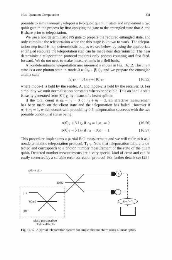
16.4 Quantum Computation 331
possible to simultaneously teleport a two qubit quantum state and implement a twoqubit gate in the process by first applying the gate to the entangled state that A andB share prior to teleportation.
We use a non deterministic NS gate to prepare the required entangled state, andonly complete the teleportation when the this stage is known to work. The telepor-tation step itself is non deterministic but, as we see below, by using the appropriateentangled resource the teleportation step can be made near deterministic. The neardeterministic teleportation protocol requires only photon counting and fast feed-forward. We do not need to make measurements in a Bell basis.
A nondeterministic teleportation measurement is shown in Fig. 16.12. The clientstate is a one photon state in mode-0 α|0〉0 + β|1〉0 and we prepare the entangledancilla state
|t1〉12 = |01〉12 + |10〉12 (16.55)
where mode-1 is held by the sender, A, and mode-2 is held by the receiver, B. Forsimplicity we omit normalisation constants wherever possible. This an ancilla stateis easily generated from |01〉12 by means of a beam splitter.
If the total count is n0 + n1 = 0 or n0 + n1 = 2, an affective measurementhas been made on the client state and the teleportation has failed. However ifn0 + n1 = 1, which occurs with probability 0.5, teleportation succeeds with the twopossible conditional states being
α|0〉2 + β|1〉2 if n0 = 1,n1 = 0 (16.56)
α|0〉2−β|1〉2 if n0 = 0,n1 = 1 (16.57)
This procedure implements a partial Bell measurement and we will refer to it as anondeterministic teleportation protocol, T1/2. Note that teleportation failure is de-tected and corresponds to a photon number measurement of the state of the clientqubit. Detected number measurements are a very special kind of error and can beeasily corrected by a suitable error correction protocol. For further details see [28]
Fig. 16.12 A partial teleportation system for single photons states using a linear optics

332 16 Quantum Information
The next step is to use T1/2 to effect a conditional sign flip csign1/4 which suc-ceeds with probability 1/4. Note that to implement csign on two bosonic qubits inmodes 1,2 and 3,4 respectively, we can first teleport the first modes of each qubitto two new modes (labelled 6 and 8) and then apply csign to the new modes. Whenusing T1/2, we may need to apply a sign correction. Since this commutes with csign,there is nothing preventing us from applying csign to the prepared state before per-forming the measurements. The implementation is shown in Fig. 16.13 and nowconsists of first trying to prepare two copies of |t1〉 with csign already applied, andthen performing two partial Bell measurements. Given the prepared state, the prob-ability of success is (1/2)2. The state can be prepared using csign1/16, which meansthat the preparation has to be retried an average of 16 times before it is possible toproceed.
To improve the probability of successful teleportation to 1−1/(n + 1), we gen-eralise the initial entanglement by defining
|tn〉1...2n =n
∑j=0|1〉 j|0〉n− j|0〉 j|1〉n− j . (16.58)
The notation |a〉 j means |a〉|a〉 . . ., j times. The modes are labelled from 1 to 2n,left to right. Note that the state exists in the space of n bosonic qubits, where the kthqubit is encoded in modes n + k and k (in this order).
To teleport the state α|0〉0 + α|1〉0 using |tn〉1...2n we first couple the client modeto half of the ancilla modes by applying an n + 1 point Fourier transform on modes0 to n. This is defined by the mode transformation
Q1
Q2
2
5
6
8
7
3
0
0
1
0
1
1
1
0
–45°
–45°
–45°
45°
45°
45°
NS–1
NS–1 10
10
n (R1)
(R5)
(R7)
(R3)
C1
C1
n
n
n
4
1
Fig. 16.13 A CSIGN two qubit gate with teleportation to increase success probability to 1/4.When using the basic teleportation protocol (T1), we may need to apply a sign correction. Sincethis commutes with CSIGN, it is possible to apply CSIGN to the prepared state before performingthe measurements, reducing the implementation of CSIGN to a state-preparation (outlined) andtwo teleportations. The two teleportation measurements each succeed with probability 1/2, givinga net success probability of 1/4. The correction operations C1 consist of applying the phase shifterwhen required by the measurement outcomes

16.4 Quantum Computation 333
ak→ 1√n + 1
n
∑l=0
ωklal (16.59)
where ω = ei2π/(n+1) This transformation does not change the total photon numberand is implementable with passive linear optics. After applying the Fourier trans-form, we measure the number of photons in each of the modes 0 to n. If the mea-surement detects k bosons altogether, it is possible to show [28] that if 0 < k < n+1,then the teleported state appears in mode n + k and only needs to be corrected byapplying a phase shift. The modes 2n− l are in state 1 for 0 ≤ l < (n− k) and canbe reused in future preparations requiring single bosons. The modes are in state 0for n− k < l < n. If k = 0 or k = n + 1 an effective measurement of the client ismade, and the teleportation fails. The probability of these two events is 1/(n + 1),regardless of the input. Note that again failure is detected and corresponds to mea-surements in the basis |0〉, |1〉with the outcome known. Note that both the necessarycorrection and the receiving mode are unknown until after the measurement.
The linear optics quantum computing (LOQC) model described above can bedrastically simplified by adopting the cluster state method of quantum computation[29]. The cluster state model was developed by Raussendorf and Breigel [30] and isquite different from the circuit models that we have been using. In cluster state QC,an array of qubits is initially prepared in a special entangled state. The computa-tion then proceeds by making a sequence of single qubit measurements. Each mea-surement is made in a basis that depends on prior measurement outcomes. Nielsenrealised that the LOQC mode of [28] could be used to efficiently assemble the clus-ter using the nondeterministic teleportation tn. As we saw the failure mode of thisgate constituted an accidental measurement of the qubit in the computational basis.The key point is that such an error does not destroy the entire assembled cluster butmerely detaches one qubit from the cluster. This enables a protocol to be devisedthat produces a cluster that grows on average. The LOQC cluster state method dra-matically reduces the number of optical elements required to implement the originalLOQC scheme. Of course if large single photon Kerr nonlinearities were available,the optical cluster state method could be made deterministic [31].
A number of LOQC protocols have been implemented in the laboratory. The firstexperiment was performed by Pittmann and Franson [32]. This used entangled an-cillas that are readily produced as photon pairs in a spontaneous parametric downconversion process. A simplified version of the LOQC model was implemented byO’Brien et al. [33], based on a proposal of Ralph et al. [34] for a CNOT gate shownin Fig. 16.14. The simplification results by firstly setting the beam splitter parame-ters θ1,θ3 to zero in the NS gate implementation and secondly only detecting photoncoincidences at the output. This gate performs all the operations of a CNOT gate butrequires only a two photon input. Detecting only coincidences means that the de-vice must be configured so that correct operation leads to a coincidence detectionof both photons at the output. The gate is non deterministic but gate failures aresimply not detected at all. In essence, the control (C) and target (T) qubits act astheir own ancilla. When the control is in the logical one state, the control and tar-get photons interfere non-classically at the central 1/3 beam splitter which causes

334 16 Quantum Information
Fig. 16.14 A simplifiedCNOT gate that gives cor-rect operation only when bothinput photons are detectedcoincidentally at the output
1/3
1/2 1/2
1/3
1/3
{{
}}
Cin Cout
ToutTin
discard
discard
a π phase-shift in the upper arm of the central interferometer and the target statequbit is flipped. The qubit value of the control is unchanged. Successful operationis heralded by coincidence detection of both photons and success will occur withprobability 1/9.
In the UQ experiment the two modes of each qubit are distinguished by orthogo-nal polarisations. This may be converted to spatial mode encoding by using polaris-ing beam splitters and a half wave plate, as shown in Fig. 16.15. The key advantagein using a gate based on two photon coincidence detection is that spontaneous para-metric down conversion (SPDC) may be used in place of true single photon sources.An SPDC produces a photon pair in two distinct spatio-temporal modes at randomtimes. There is a small probability of producing more than two photons, but this canbe neglected.
The truth table for a CNOT operation was experimentally determined by prepar-ing each of the four possible input states to the gate, CT 〉 = |00〉, |11〉, |10〉, |01〉.A comparison of the experimental results and the ideal CNOT gate are shown inFig. 16.14. A single classical interference event is required when the control is in
Statepreparation
PBS BS
X
X
QWP HWP SPCM
“1/3”(62.5°)
Automated quantumstate tomography
X Dump702.2+ 0.18 nm filter–
Cin
C0 Cout
Tout
Cs
T+
T–
Tin
Fig. 16.15 The optical design schematic of the polarisation encoding implementation of the exper-iment of O’Brien et al., PBS: polarising beam splitter, QWP: quarter wave plate, HWP: half waveplate, SPCM: single photon counting module and X: beam dump. Reproduced, with permission,from Nature, 426, 264 (2003)

16.4 Quantum Computation 335
state |0〉L and experimentally the correct output is obtained in roughly 95% of cases.In the case of the control in state |1〉L, correct operation is obtained in only 75% ofcases as this situation requires a non classical interference event for which verycareful mode matching is required.
While this provides good evidence the gate is working the key test of a quantumCNOT gate is that it produce maximally entangled states when the control is in a su-perposition of the two logical states. For example if the control is in state |0〉L−|1〉L,while the target is in 1〉L, the two-qubit output state is |ψ−〉= |01〉L−|10〉L (where|xy〉L = |x〉L⊗ |y〉L, with the first factor the control qubit and the second factor thetarget). In testing the truth table, the output logical states were measured in the log-ical basis. Such a “computational basis” measurement of course will not reveal theclassical correlation imposed by the truth table but not quantum coherence. To seethe quantum coherence implicit in the entangled state we need to measure in a basisother than the computational basis. In the experiment this was done by measuringthe coincidence count rate while using a half wave plate set to pass control photonsin either of the states |0〉L or state |0〉L + |1〉L. The experimental results are showin Fig. 16.16. The visibilities in the two curves are greater than 90% which is thesignature of entanglement in the output state.
An even better diagnostic of the gate operation is provided by state tomography,a reconstruction of the full density matrix of the output state [35], when the outputis entangled. State tomography requires sampling the statistics for the measurementoutcomes of 16 different two qubit projections. Given these statistics data inversioncan be devised to reconstruct the density matrix for the output state. Given the den-sity matrix, we can then compute its overlap, or fidelity, with respect to the pureideal entangled state |ψ−〉 that the ideal gate would produce. In the case of |ψ−〉the fidelity obtained in the experiment was 0.87± 0.08. This is sufficiently highthat such a state were it not destroyed in the detection process, would violate a Bellinequality test.
More recent experiments have improved on these early experiments. An NS gateclose to the original proposal, was implemented in the Zeilinger group, using a po-larisation encoding and the four photon state emitted by spontaneous parametricdown conversion [36]. As in the UQ experiment, a coincidence detection configura-tion was used to signal correct operation of the gate. The experimentally observed
Fig. 16.16 Conditionalcoincidence rtes for non-orthogonal measurementbases. The control analyserwas set to pass |0〉L + |1〉L(circles) and |0〉L (triangles)when the input to the controlis (|0〉L−|1〉L) and the inputto the target is |1〉L. Repro-duced, with permission, fromNature, 426, 264 (1003)
1,400
1,200
1,000
800
600
400
200
00 20 40 60 80
Target HWP (degrees)
Coi
ncid
ence
s pe
r 10
s

336 16 Quantum Information
conditional phase shift was 1.05±0.06π. Future progress on linear optical quantumcomputing schemes will most likely be based on cluster state implementations. Afour photon cluster state implementation was recently implemented by the Zeilingergroup [37].
16.4.2 Single Photon Sources
As we have seen both QKD and LOQC motivate the development of single photonsources. Single photon sources enable QKD to escape beam splitter attacks that arepossible with weak coherent pulses. In order to progress to scaleable architectures,LOQC will certainly require the development of good single photons sources andhighly efficient single photon detectors that can in fact discriminate between 0,1and 2 photons. Fortunately steady progress is being made on both technologies. Therequirements on single photon sources are much more demanding than those forsingle photon sources in QKD and we now briefly discuss some of these.
What we need is an optical pulse source in which each pulse contains one andonly one photon. Clearly such a source is going to produce photon antibunchingand the g(2)(τ) (see Sect. 3.6) is clearly a key diagnostic for such a source. Howevera more stringent requirement is the ability of such a source to produce a strongHong-Ou-Mandle interference dip. (See Exercise 3.4(c)).
In order to define single photon states, let us begin by defining the positive fre-quency field component as,
a(t) =∞
∑n=1
ane−int (16.60)
The allowed wave vectors for plane wave modes in a box of length L, form a de-numerable set given by kn = nπ
L with corresponding frequencies ωn = ckn. If wemeasure time in units of πL/c, the allowed frequencies may simply be denoted byan integer ωn = n = 1,2, . . .. The Bose annihilation and creation operators obey theusual commutation relations. Following the standard theory of photo-detection (seeSect. 3.10) the probability per unit time for detecting a single photon is given byp1(t) = γn(t) where n(t) = 〈a†(t)a(t)〉 and the parameter γ characterises the detec-tor. A single-photon state may be then defined as
|1; f 〉=∞
∑m=1
fma†m|0〉 (16.61)
where |0〉= ∏m |0〉m is the multimode global vacuum state, and we require that thesingle photon amplitude, fm satisfies
∞
∑m=0
| fm|2 = 1 (16.62)

16.4 Quantum Computation 337
The counting probability is then determined by
n(t) =
∣∣∣∣∣∞
∑k=1
fke−ikt
∣∣∣∣∣2
(16.63)
This function is clearly periodic with a period 2π. As the spectrum is bounded frombelow by n = 1, it is not possible to choose the amplitudes fn so that the functionsn(t) have arbitrarily narrow support on t ∈ [0,2π).
While a field for which exactly one photon is counted in one counting interval,and zero in all others, is no doubt possible, it does not correspond to a more physicalsituation in which a source is periodically producing pulses with exactly one pho-tons per pulse. To define such a field state we now introduce time-bin operators. Forsimplicity we assume that only field modes n ≤ N are excited and all others are inthe vacuum state. It would be more physical to assume only field modes are excitedin some band, Ω−B ≤ n ≤ Ω + B. Here Ω is the carrier frequency and 2B is thebandwidth. However this adds very little to the discussion.Define the operators
aν =1√N
N
∑m=1
e−iτmν am (16.64)
where τ = 2πN This can be inverted to give
am =1√N
N
∑ν=1
eiτmν aν (16.65)
The temporal evolution of the positive frequency components of the field modesthen follows from (16.60)
a(t) =N
∑μ=1
gμ(t)aμ (16.66)
where
gμ(t) =1√N
[1− ei(ντ−t)
]−1(16.67)
The time-bin expansion functions, gμ(t) are a function of ντ− t alone and are thussimple translations of the functions at t = 0. The form of (16.66) is a special caseof a more sophisticated way to define time-bin modes. If we were to regard a(t)as a classical signal then the decomposition in (16.66) could be generalised as awavelet transform where the integer μ labels the translation index for the waveletfunctions. In that case the functions gμ(t) could be made rather less singular. Inan experimental context however the form of the functions gμ(t) depends upon thedetails of the generation process.
The linear relationship between the plane wave modes am and the time bin modesaν is realised by a unitary transformation that does not change particle number, sothe vacuum state for the time-bin modes is the same as the vacuum state for theglobal plane wave modes. We can then define a one-photon time-bin state as
338 16 Quantum Information
˜|1〉ν = a†ν |0〉 (16.68)
The mean photon number for this state is,
n(t) = |gν(t)|2 (16.69)
This function is periodic on t ∈ [0,2π) and corresponds to a pulse localised in timeat t = ντ. Thus the integer ν labels the temporal coordinate of the single photonpulse.
We are now in a position to define an N-photon state with one photon per pulse. Inaddition to the mean photon number, n(t) we can now compute two-time correlationfunctions such as the second order correlation function, G(2)(τ) defined by
G(2)(T ) = 〈a†(t)a†(t + T)a(t + T)a(t)〉 (16.70)
The simplest example for N = 2 is
|1μ ,1ν〉= a†μ a†
ν |0〉 μ �= ν (16.71)
The corresponding mean photon number is
n(t) = |gμ(t)|2 + |gν(t)|2 (16.72)
as would be expected. The two-time correlation function is,
G(2)(τ) = |gμ(t)gν(t + T)+ gν(t)gμ(t + T )|2 (16.73)
Clearly this has a zero at T = 0 reflecting the fact that the probability to detect a sin-gle photon immediately after a single photon detection is zero, as the two pulses areseparated in time by |μ−ν|. This is known as anti-bunching and is the first essen-tial diagnostic for a sequence of single photon pulses with one and only one photonper pulse. When T = |μ − ν|τ however there is a peak in the two-time correlationfunction as expected.
An example of such a single photon source producing a second order two-timecorrelation function of this kind was implemented by the group of Yamamoto [38].The source was based on spontaneous emission from exciton recombination froma single InAs quantum dot in a micropillar cavity using distributed Bragg reflect-ing mirrors. The devices operate at low temperature (3− 7 K) and are pumpedby a pulsed TiSi laser with 3 ps pulses every 13 ns. Three quantum dots were re-ported producing light with wavelengths 931,932 and 937 nm. In Fig. 16.17 weshow the experimental results for the second order two time correlation functionusing a Hanbury-Brown and Twiss configuration.
We now consider an interferometer with single photon input states. The most rel-evant example for LOQC protocols is the Hong-Ou-Mandel (HOM) interferometer.This example has been considered by Rohde and Ralph [39]. In this case two fields,distinguished by momentum or polarisation are coupled by a linear optical device(referred to for simplicity as a beam-splitter). After the interaction, each field is

16.4 Quantum Computation 339
400
200Cou
nts
00
τ = t2 – t1 (ns)50 100 150
Fig. 16.17 The photon correlation histogram for emission form a single exciton quantum dot.The results were obtained using a Hanbury-Brown and Twiss experiment. The emission from thequantum dot was split into two paths via a beam splitter and each path directed towards a photondetector. The number of events in which a photon was detected on one detector at time t1 and onthe other detector at time t2 = t1 + τ. The suppression of the peak at zero delay is characteristic ofa single photon pulse source. (From [38]) reproduced with permission from Nature
directed onto a photon counter, and the probability for a coincidence count is deter-mined. We label the two sets of modes by the latin symbols a,b so for example thepositive frequency parts of each field are simply a(t),b(t). The coupling betweenthe modes is described by a scattering matrix connecting the input and output planewaves
aoutn =
√ηan +
√1−ηbn (16.74)
boutn =
√ηbn−
√1−ηan (16.75)
where 0≤ η≤ 1. This is realised by a unitary transformation, U , for example, aoutn =
U†anU . The total photon number at the input is N(t) = 〈a†(t)a(t)〉+ 〈b†(t)b(t)〉.It is easy to see that this is unchanged by the beam-splitter transformation. Theprobability, per unit time, for there to be a coincident detection of a single photon ateach output beam is easily seen to be proportional to
C = 〈a†(t)b†(t)b(t)a(t)〉 (16.76)
The overline represents a time average over a detector response time that is longcompared to the period of the field carrier frequencies. In this example we onlyneed consider the case of one photon in each of the two distinguished modes, so wetake the input state to be
|1〉a⊗|1〉b =∞
∑m,n=1
αnβma†nb†
m|0〉 (16.77)
where αn,βn refer to the excitation probability amplitudes for modes an,bn re-spectively. This state is transformed by the unitary transformation, U , to give|ψ〉out = U |1〉a⊗ |1〉b. In the case of a 50/50 beam splitter, for which η = 0.5, thisis given as

340 16 Quantum Information
|ψ〉out =∞
∑n,m=1
αnβmUa†nb†
m
=12
∞
∑n,m=1
αnβm(a†n + b†
n)(b†m−a†
m)|0〉
=12
∞
∑n,m=1
αnβm[|1〉an |1〉bm −|1〉an|1〉am |0〉b
+|1〉bn |1〉bm |0〉a−|1〉bn |1〉am ]
Note that the second and third terms in this sum have no photons in modes b and arespectively. We then have that
C =12− 1
2
∞
∑n,m=1
αnα∗mβmβ∗n (16.78)
If the excitation probability amplitudes at each frequency are identical, αn = βnthis quantity is zero. In other words only if the two-single photon wave packets areidentical do we see a complete cancellation of the coincidence probability. This isthe second essential diagnostic for a single photon source. Of course in an exper-iment complete cancellation is unlikely. The extent to which the coincidence rateapproaches zero is a measure of the quality of a single photon source as far asLOQC is concerned. Whether or not this is the case depends on the nature of thesingle photon source.
In Fig. 16.18 we show the results of a HOM interference experiment using theexciton quantum dot source of Yamamoto [38].
Currently the two schemes used to realise single photon sources are: I conditionalspontaneous parametric down conversion, II cavity-QED Raman schemes. As dis-cussed by Rohde and Ralph, type-I corresponds to a Gaussian distribution of αn asa function of n. The second scheme, type-II, leads to a temporal pulse structure that
delay time (ns)0
0.25
0.50
coin
cide
nce
prob
abili
ty
Fig. 16.18 The coincidence count probability for two photons incident on a beam splitter as a func-tion of the time delay in arrival times of the photons at the beam splitter for the exciton quantumdot source of Santori et al. [38]. Reproduced with permission from Nature

16.4 Quantum Computation 341
is the convolution of the excitation pulse shape and the Lorentzian line shape of acavity. If the cavity decay time is the longest time in the dynamics, the distributionαn takes a Lorentzian form.
As an example of the experimental constraints on the generation of single photonstates we now review an example of a cavity-QED Raman scheme implemented byKeller et al. [40]. Photon anti-bunching from resonance fluorescence was discussedin Sect. 10.3. If an atom decays spontaneously from an excited to a ground state,a single photon is emitted and a second photon cannot be emitted until the atom isre-excited. Unfortunately the photon is emitted into a dipole radiation pattern over acomplete solid angle. Clearly we need to engineer the electromagnetic environmentwith mirrors, dielectrics, etc, to be sure a preferred mode for emission. Howeversingle photon sources based on spontaneous emission are necessarily compromisedby the random nature of spontaneous emission. The decay process is a conditionalPoison process. This means that after a fast excitation pulse there is a small randomtime delay in the emission of the photon. This leads to time jitter in the single photonpulse period. A similar situation prevails in the case of single exciton sources [38],where spontaneous recombination leads to time jitter for the same reason. Clearlywhat we need is a stimulated emission process not a spontaneous emission process.A number of schemes based on stimulated Raman emission into a cavity mode havebeen proposed to this end [40, 41, 42].
Consider a three-level atomic system in Fig. 16.19. The ground state is coupledto the excited state via a two-photon Raman process mediated by a well detunedthird level. In this experiment a calcium ion ( 40Ca+) was trapped in a cavity via anrf ion trap. The cavity field is nearly resonant with the 42P1/2→ 32D3/2 transition.Initially there is no photon in the cavity. An external laser is directed onto the ionand is nearly resonant with the 42P1/2→ 42P1/2 transition. When this laser is on, theatom can be excited to the 32D3/2 level by absorbing one pump photon and emittingone photon into the cavity. This is a stimulated Raman process and thus time ofemission of the photon into the cavity is completely controlled by the temporalstructure of the pump pulse. The photon in the cavity then decays through the endmirror, again as a Poisson process this time at a rate given by the cavity decay rate.This can be made very fast.
In principle one can now calculate the probability per unit time to detect a singlephoton emitted from the cavity. If we assume every photon emitted is detected, this
Fig. 16.19 A possible three-level atomic system for atwo-photon Raman singlephoton source. The pumpbeam is a strong classicalcoherent pulse. The cavityfield is an intracavity fieldmode initially prepared in avacuum state
pump
42P1/2
32D3/2
42S1/2
cavity

342 16 Quantum Information
probability is simply p1(t) = κ〈a†(t)a(t)〉 where κ is the cavity decay rate and a,a†
are the annihilation and creation operators for the intracavity field and
〈a†(t)a(t)〉= tr(ρ(t)a†a) (16.79)
where ρ(t) is the total density operator for ion-plus-cavity-field system. This maybe obtained by solving a master equation describing the interaction of the electronicstates of the ion and the two fields, one of which is the time dependent pump. Ofcourse for a general time-dependent pump pulse-shape this can only be done nu-merically. Indeed by carefully controlling the pump pulse shape considerable con-trol over the temporal structure of the single photon detection probability may beachieved. In the experiment of Keller et al. [40] the length of the pump pulse wascontrolled to optimise the single photon output rate. The efficiency of emission wasfound to be about 8%, that is to say, 92% of pump pulses did not lead to a single-photon detection event. This was in accordance with the theoretical simulations.These photons are probably lost through the sides of the cavity. It is important tonote that this kind of loss does not effect the temporal mode structure of the emitted(and detected) photons.
In a similar way we can compute the second order correlation function via
G(2)(T ) = κ2tr(a†aeL T (aρ(t)a†) (16.80)
where eL T is a formal specification of the solution to the master equation for a timeT after the “initial” conditional state aρ(t)a†. Once again, due to the non stationarynature of the problem, this must be computed numerically. However if the pumppulse duration is very short compared to the cavity decay time and further the cavitydecay time is the fastest decay constant in the system, the probability amplitude toexcite a single photon in a frequency at frequency ω is very close to Lorentzian. Theexperiment of Keller et al. [40] revealed a clear suppression of the peak at T = 0in the (normalised) correlation function g(2)(T ), thus passing the first test of a goodsingle photon source.
A very different approach to single photon sources is based on the spontaneousparametric down conversion using a crystal with a significant second order opticalnon linearity. In these systems, a pair of photons is produced simultaneously, but atrandom times. However if we detect one photon of the pair in a given time window,we know the temporal coordinates of the other photon. A detailed study of the modestructure of the conditional photon pulse has been undertaken by Walmsley and co-workers [43]. To a very good approximation the probability amplitude functions,αω, are Gaussian with variance depending ultimately on the filters used in the con-ditioning detection step. These sources have been the sources of choice for the earlyimplementations of LOQC. However the random time of pair production means thatthe single photons are heralded but not produced on-demand. An ingenious schemeto overcome this limitation is being pursued by the NIST group of Migdall [44]. Intheir scheme a large number of conditional sources are multiplexed, together withfast electro-optical switching, so that at some repetition rate and detection band-width, there is near determinant sequence of singe photon detection events.

Exercises 343
Exercises
16.1 Consider the following EPR entangled state of two modes A and B,
|X ,Y 〉AB = e−i2 YAXB |X〉A⊗|Y〉B (16.81)
where the states appearing on the left hand side of this equation are thequadrature phase eigenstates. Verify that this state is a simultaneous eigen-state of XA− XB and YA + YB with respective eigenvalues, X ,Y .
16.2 The two-mode squeezed vacuum state, (16.16), is also entangled with respectto the correlation specified by the statement: an equal number of photons ineach mode. However it is not a perfectly entangled state, which would requirethe (unphysical) case of a uniform distribution over correlated states. Showthat the state is an eigenstate of the photon number difference and the phasesum. To show this compute the canonical joint phase distribution P(φA,φB),for the two modes using the projection operator valued measure (see Sect.2.8). Show that as λ→ 1 this distribution becomes very sharply peaked atφA = −φB. Thus the photon number in each mode are perfectly correlatedwhile the phase in each mode is highly anti correlated.
16.3 Joint quadrature phase measurement of XC− XA and YC +YA are made on twomodes, A and C, with the results X ,Y respectively. Show that the conditionalstate resulting from this joint quadrature measurement is described by theprojection onto the state |X ,Y 〉CA where
|X ,Y 〉CA = e−i2 XAYC |X〉C⊗|Y 〉A (16.82)
16.4 In the protocol for teleportation based on the state in Exercise 16.1, let thetotal input state for the teleportation protocol be
|ψ〉in = |ψ〉C⊗|X0,Y0〉AB (16.83)
Joint quadrature phase measurements of XC − XA and YC + YA are made onthe client and sender modes C and A, yielding two real numbers, X ,Y respec-tively. Show that the conditional state of mode B after the measurement onsender and the client, in the special case of X0 = Y0 = 0, is then given by
|φ(X ,Y )〉B = ei2 XY e
i2 XYB e−
i2 Y XB |ψ〉B (16.84)
16.5 Consider the beam splitter unitary transformation U = eθ(a†2a1−a2a†
1). Showthat
2〈0|U(θ)|0〉2 =∞
∑n=0
(cosθ−1)n
n!(a†
1)nan
1
2〈1|U(θ)|1〉2 = cos ϒ(0)− sin2 θa†1ϒ(0)a1

344 Quantum Information
16.6 A linear optical device acting on N modes may be described by a unitarytransformation of the form
U(H) = exp[−i�a†H�a] (16.85)
where
�a =
⎛⎜⎜⎜⎜⎜⎜⎜⎜⎜⎜⎝
a1
a2...
aN
aN...
aN
⎞⎟⎟⎟⎟⎟⎟⎟⎟⎟⎟⎠
(16.86)
and H is a hermitian matrix. Show that this transformation leaves the totalphoton number invariant,
U†(H)�a† ·�aU(H) =�a† ·�a (16.87)
and induces a linear unitary transformation on the vector�a as
U†(H)�aU(H) = S(H)�a (16.88)
16.7 Consider the three mode optical device shown in Fig. 16.10. Mode a1 is thesignal mode prepared in an arbitrary two photon state |ψ〉. Modes a2,a3 areancilla modes prepared in the photon number states |1〉2 and |0〉3, respec-tively. Using the notation of Exercise 16.6, let the S(H) be the orthogonalmatrix with matrix elements si j. Show that the (unormalised) conditional stateof the signal mode, conditioned on counting one photon on mode a2 and nophotons in mode a3 is given by |upsi′〉 = E|ψ〉 with E = s22A + s12s21a†
1Aa1
where A = ∑∞n=0
(s11−1)n
n! (a†1)
nan1. Verify that, for the choice given in Fig.
16.10, this implements a conditional sign shift gate with probability of 0.25 .
References
1. C.E. Shannon: Bell System. Tech. J. 27, 379 (1948); Reprinted in, C.E. Shannon, W. Weaver:The Mathematical Theory fo Communication (The University of Illinois Press, Urbana 1949)
2. R.B. Ash: Information Theory (Dover, New York 1965)3. Charles H. Bennett 1, David P. DiVincenzo 1, Christopher A. Fuchs, Tal Mor, Eric Rains, Peter
W. Shor, John A. Smolin, William K. Wootters: Quantum Nonlocality Without Entanglement,quant- ph/ 9804053 v4 2 Nov 1998

References 345
4. A. Peres: Phys. Rev. Lett 77, 1413 (1996)5. G. Adesso, F. Illuminati: Phys. Rev. A 72, 032334 (2005)6. I. Bengtsson, K. Zyczkowski, “Geometry of Quantum States”, pp. 333, Cambridge University
press (Cambridge, 2006)7. S. Wiesner: “Conjugate Coding,” SIGACT News 15, 78 (1983)8. C.H. Bennett, G. Brassard: “Quantum Cryptography: Public Key Distribution and Coin Toss-
ing,” Proceedings of IEEE International Conference on Computers, Systems and Signal Pro-cessing, Bangalore (New York, IEEE 1984)
9. C.H. Bennett, G. Brassard: “The Dawn of a New Era for Quantum Cryptography: The Ex-perimental Prototype is Working,” SIGACT NEWS 20 (4), 78 (1989); C.H. Bennett et al.:Experimental Quantum Cryptography, J. Crypto. 5, 3 (1992)
10. A. Muller, J. Breguet, N. Gisin: Europhys. Lett. 23, 383 (1993)11. A.K. Ekert: Quantum Cryptography Based on Bell’s Theorem, Phys. Rev. Lett. 67, 661 (1991)12. C.H. Bennett: Quantum Cryptography Using Any Two Non-Orthogonal States, Phys. Rev.
Lett. 68, 3121 (1992)13. W.K. Wootters, W.H. Zurek: Nature 299, 802 (1982); D. Dieks: Phys. Let. A, 92, 271 (1982)14. R.J. Hughes, W.T. Buttler, P.G. Kwiat, G.G. Luther, G.L. Morgan, J.E. Nordholt,
C.G. Peterson, C.M. Simmons: Proc. SPIE 3076, 2 (1997)15. P.A. Hiskett et al., New Journal of Physics, 8, 193 (2006)16. C.H. Bennett, G. Brassard, C. Crepeau, R. Jozsa, A. Peres, W.K. Wooters: Phys. Rev. Lett. 70,
1895 (1993)17. B. Schumaker: Phys. Rev. A 51, 2783 (1995)18. A. Furasawa, J.L. Sørensen, S.L. Braunstein, C.A. Fuchs, H.J. Kimble, E.S. Polzik: Science,
282, 23 October, 706, (1998)19. S.L. Braunstein, H.J. Kimble: Phys. Rev. Letts. 80, 869 (1998)20. L. Vaidman: Phys. Rev. A 49 1473 (1994)21. refer to di Martini teleportation experiment22. refer to Zeilinger teleportation experiment23. Richard P. Feynman: Simulating Physics with Computers, Int. J. Theoretical Phys., 21, 467
(1982)24. D. Deutsch: Quantum-Theory, the Church-Turing Principle and the Universal Quantum Com-
puter. Proc. R. Soc. Lond. A 400, 97–117 (1985)25. P. Shor: Algorithms for Quantum Computation: Discrete Logarithms and Factoring. Proc. 35th
Annual Symposium on Foundations of Computer Science (1994). See also LANL preprintquant-ph/9508027
26. Richard Cleve, Artur Ekert, Leah Henderson, Chiara Macchiavello and Michele Mosca: Onquantum algorithms, Complexity, 4, 33 (1999)
27. D. Gottesman, I.L. Chuang: Nature, 402, 390–393 (1999)28. E. Knill, R. Laflamme, G.J. Milburn: Nature, 409, 46, (2001)29. Michael A. Nielsen: Phys. Rev. Lett. 93, 040503 (2004)30. R. Raussendorf, H.J. Briegel: Phys. Rev. Lett. 86, 5188 (2001)31. G.D. Hutchinson, G.J. Milburn: J. Mod. Opt. 51, 1211–1222 (2004)32. T.B. Pittman, B.C. Jacobs, J.D. Franson: Phys. Rev. A 64, 062311 (2001)33. J.L. OBrien, G.J. Pryde, A.G. White, T.C. Ralph, D. Branning: Nature, 426, 264 (2003)34. T.C. Ralph, N.K. Langford, T.B. Bell, A.G. White: Phys. Rev. A 65, 062324 (2002)35. D.F.W. James, P.G. Kwiat, W.G. Munro, A.G. White: Phys. Rev. A64, 052312 (2001)36. K. Sanaka,T. Jennewein, Jian-Wei Pan, K. Resch, A. Zeilinger: Phys. Rev. Lett. 92, 017902–1
(2004)37. P. Walther, K.J. Resch, T. Rudolph, E. Schenck, H. Weinfurter, V. Vedral, M. Aspelmeyer,
A. Zeilinger: Nature, 434, 169 (2005)38. C. Santori, D. Fattal, J. Vuckovic, G.S. Solomon, Y. Yamamoto: Nature, 419, 594, (2002)39. P.P. Rohde, T.C. Ralph: PRA 71, 032320 (2005)40. M. Keller, B. Lange, K. Hayasaka, W. Lange, H. Walther: Nature, 431, 1075 (2003)41. M. Hennrich, T. Legero, A. Kuhn, G. Rempe: New J. Phys. 6, 86 (2004)

346 Quantum Information
42. Christian Maurer, C. Becher, C.s Russo, J. Eschner, R. Blatt: New J. Phys. 6, 94(2004)43. W.P. Grice et al.: Physical Review A, 64, 063815 (2001)44. A.L. Migdall, D. Branning, S. Castelletto, M. Ware: SPIE Free-Space Laser Communication
and Laser Imaging II. To Appear in the Proceeding of SPIE Free-Space Laser Communicationand Laser Imaging II, Proc. of the SPIE, 4821, 455–465, 2002
Further Reading
Nielsen M., I. Chuang: Quantum Computation and Quantum Information (Cambridge Universitypress, Cambridge 2000)
Bouuwmester D., A. Ekert, A. Zeilinger: (eds) The Physics of Quantum Information (Springer,Berlin 2000)
Hoi-Kwong Lo, Tim Spiller, Sandu Popescu: Introduction to Quantum Computation and Informa-tion (World Scientific, Singapore 1998)
Loepp S., W.K. Wootters: Protecting Information: From Classical Error Correction to QuantumCryptography (Cambridge University Press, New York 2006)
Gisin N., G. Ribordy, W. Tittel H. Zbinden: Quantum Cryptography Rev. Mod. Phys. 74, 145(2002)
Chapter 17Ion Traps
17.1 Introduction
Ion trap technology currently leads the way in the effort to gain complete control ofquantum coherence in isolated systems. The seminal paper of Cirac and Zoller thrustthe technology to the forefront of the quantum processing agenda in a seminal paperin 1995 [1]. Beginning over 30 years ago, experimentalists began trapping clouds ofatomic ions in order to achieve higher spectroscopic resolution [2]. The heritage ofthis effort is the current ability to define time standards using ion trap clocks. Futuredevelopments will depend on the ability to make smaller trap arrays for quantumcomputing applications.
Ion trap technology also enables quantum limited measurements of the electronicand vibrational states of a single trapped ion using the method of cycling fluorescenttransitions. This ability led to a complete reappraisal of how quantum mechanics ofsingle systems, subject to continuous observation, should be interpreted [3] enablingan explicit physical demonstration of the concept of a quantum trajectory discussedin Chap. 6. It is possible to trap and cool a single ion close to its vibrational groundstate [4], carefully prepare complex superpositions ofenergy eigenstates through opti-cal excitation and then monitor thesubsequent dynamicswith extaordinary sensitivity.
17.2 Trapping and Cooling
Laplace’s equation indicates that it is not possible to trap a charged particle in threedimensions with a static potential: there is always one unstable (untrapped) directionin an electrostatic potential. We must resort to time periodic potentials. In Fig. 17.1we show a possible configuration of electrodes.
The time dependent potential can be written
V (x,y,z,t) =V2
(kxx2 + kyy2 + kzz2)+
12
V cos(ωr f t)(k′xx2 + k′yy2) (17.1)
347

348 17 Ion Traps
RF
+DC
RF
+DC
+DC
+DC
-DC
-DC
y x
z axis(trap axis)
z-axis
Fig. 17.1 A schematic representation of a linear radio frequency ion trap (after [5])
where ωr f is the frequency of the time dependent potential. Laplace’s equation im-plies, kx + ky + kz = 0, k′x + k′y = 0. If we assume [5]
ax =4Z|e|V kx
mω2r f
<< 1
qx =2Z|e|Vk′x
mω2r f
<< 1
then the motion in the x-direction is approximately harmonic, as is motion in they-direction. Given isotropy in the x−y plane, so that kx = ky, k′x = k′y and the motionis harmonic with the secular frequency
ν =(ax + q2
x/2)1/2 ωr f /2 (17.2)
A small amplitude oscillatory motion at frequency ωr f is superimposed on the secu-lar motion, called the micromotion, which we neglect. In an experiment with 9Be+,the axial frequency was about 3 MHz while the transverse frequency was about8 MHz. The static potential due to end caps gives harmonic confinement along thetrap axis (z-direction). If this is kept weak, multiple ions can be trapped in a linealong the z-direction. Typically the transverse frequencies are three to four timesmore than the axial.
The centre-of-mass quantum dynamics of the ion is determined by the eigenstatesof the Hamiltonian
H = hνa†z az + hνt(a†
xax + a†yay) (17.3)

17.2 Trapping and Cooling 349
The motion is thus separable into axial and transverse motion and, to be specific, wenow concentrate on the axial motion alone. As we neglect the transverse motion, wewill drop the subscript on az,a†
z .The availability of lasers at appropriate atomic transition frequencies determine
which ions can be successfully trapped and cooled. The Wineland group at NISTColorado uses 9Be+ while the Blatt group in Innsbruck uses 40Ca+. After trappingit is necessary to remove vibrational energy from the ion, that is to say, it must becooled. The initial temperature is of the order of 104 K. The first stage of cooling isbased on Doppler cooling and is very efficient, the second stage is based on resolvedsideband cooling (see below).
The extraordinary degree of control over quantum coherence that can be achievedin an ion trap is due to a number of reasons. Firstly, it is possible to coherently couplethe vibrational motion and the internal electronic state using an external laser. Sec-ondly, resolved sideband cooling enables the vibrational motion to be prepared in itsground state with probability approaching unity. External lasers induce Raman tran-sitions between the ground and excited internal electronic state in which one phononof vibrational energy is absorbed per excitation cycle. Finally, the internal electronicstate of a single trapped ion can be determined with efficiency approaching unity bythe method of fluorescence shelving enables.
We will assume that external lasers drive a two level transition from the groundstate |g〉 to the excited state |e〉. This could be a direct dipole transition, but forquantum computing it typically involves a Raman two-photon transition connect-ing the ground state to an excited meta-stable state. In either case the Hamiltoniandescribing the system is (see 10.1),
H = hνa†a + hωAσz +hΩ2
(σ−ei(ωLt−kLq) + σ+e−i(ωLt−kLq)
)(17.4)
where q is the operator for the displacement of the ion from its equilibrium positionin the trap, ν is the trap (secular) frequency, Ω is the Rabi frequency for the twolevel transition, ωA is the atomic transition frequency, and ωL, kL are the laser fre-quency and wave number. The sigma matrices are defined in Sect. 10.1. There arethree frequencies in the problem: ν, ωA and ωL. By carefully choosing relationshipsbetween these three frequencies various quantum interactions between electron andvibrational degrees of freedom can be driven. The key point is that the phase ofthe laser field as seen by the ion depends on the position of the ion. As the ion vi-brates this phase is modulated at the trap frequency, which leads to sidebands in theabsorption spectrum for the two level system.
The ion position operator may be written,
q =(
h2mν
)1/2
(a + a†) (17.5)
We now define the Lamb-Dicke parameter, η
η = kL
(h
2mν
)1/2
= 2πΔxrms/λL (17.6)
350 17 Ion Traps
where the r.m.s position fluctuations in the oscillator ground state is Δxrms. Thenmoving to an interaction picture via the unitary transformation
U0(t) = exp[−iνa†at− iωAσzt] (17.7)
the interaction Hamiltonian can be written as
HI(t) =hΩ2
(σ− exp[−iη(ae−iνt + a†eiνt)]exp[−i(ωA−ωL)t]+ h.c
)(17.8)
The exponential of exponentials make this a complicated Hamiltonian system. How-ever in most ion trap experiments the ion is confined to a spatial region that is signif-icantly smaller than the wavelength of the exciting laser so that we may assume thatthe Lamb-Dicke parameter is small η < 1 (typically η ≈ 0.01−0.1). Expanding theinteraction to second order in the Lamb-Dicke parameter gives
HI(t) =hΩ2
[1−η2a†a](
σ−e−iδt + σ+eiδt)
−ihΩη
2
(ae−iνt + a†eiνt)e−iδtσ−+ i
hΩη2
(ae−iνt + a†eiνt)eiδtσ+
− hΩη2
4
(a2e−2iνt +(a†)2e2iνt)(e−iδtσ−+ eiδtσ+
)
where the detuning of the laser from the atomic frequency is δ = ω−ωL.Tuning the frequencies so that δ is a positive or negative integer multiple of the
trap frequency leads to resonant terms, and all time dependent terms are neglected.For carrier excitation, δ = 0, the resonant terms are
Hc = hΩ(1−η2a†a)σx carrier excitation (17.9)
where σx = (σ−+σ+)/2. If we take δ = ν so that the laser frequency is detuned be-low (to the red of) the carrier frequency by one unit of trap frequency, ωL = ωA−ν ,the resonant terms are
Hr = ihηΩ
2
(aσ+−a†σ−
)first red sideband excitation (17.10)
This is the Jaynes-Cummings Hamiltonian except that it involves the absorption ofa trap phonon as well as one laser photon. If we instead choose δ = −ν so thatωL = ωA +ν , the laser is detuned one unit of vibrational frequency above the carrier(a blue detuning), the resonant interaction Hamiltonian is
Hb = ihηΩ
2
(a†σ+−aσ−
)first blue sideband excitation (17.11)
This corresponds to an excitation process in which one photon is absorbed fromthe laser and one trap phonon is emited . We can continue to define the second redsideband excitation δ = 2ν and second blue sideband excitation δ = −2ν , and so
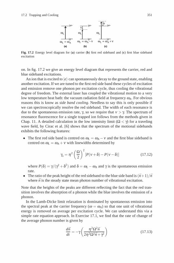
17.2 Trapping and Cooling 351
|g >
(a) (b) (c)
|e>
|g >
|e>
|g >
|e>
ωL = ωA − νωL = ωA ωL = ωA + ν
νν
ωL ωL ωL
Fig. 17.2 Energy level diagram for (a) carrier (b) first red sideband and (c) first blue sidebandexcitation
on. In fig. 17.2 we give an energy level diagram that represents the carrier, red andblue sideband excitations.
An ion that is excited to |e〉 can spontaneously decay to the ground state, enablinganother excitation. If we are tuned to the first red side band these cycles of excitationand emission remove one phonon per excitation cycle, thus cooling the vibrationaldegree of freedom. The external laser has coupled the vibrational motion to a verylow temperature heat bath: the vacuum radiation field at frequency ωA. For obviousreasons this is know as side band cooling. Needless to say this is only possible ifwe can spectroscopically resolve the red sideband. The width of each resonance isdue to the spontaneous emission rate, γ, so we require that ν > γ. The spectrum ofresonance fluorescence for a single trapped ion follows from the methods given inChap. 11. A detailed calculation in the low intenisity limit (Ω < γ) for a travelingwave field, by Cirac et al. [6] shows that the spectrum of the motional sidebandsexhibits the following features:
• The first red side band is centred on ωL = ωA−ν and the first blue sideband iscentred on ωL = ωA + ν with linewidths determined by
γs = η2(
Ω2
)2
[P(ν + δ)−P(ν− δ)] (17.12)
where P(δ) = γ/(γ2 + δ2) and δ = ωL−ωA and γ is the spontaneous emissionrate.
• The ratio of the peak height of the red sideband to the blue side band is (n+1)/nwhere n is the steady state mean photon number of vibrational excitation.
Note that the heights of the peaks are different reflecting the fact that the red tran-sition involves the absorption of a phonon while the blue involves the emission of aphonon.
In the Lamb-Dicke limit relaxation is dominated by spontaneous emission intothe spectral peak at the carrier frequency (ω = ωA) so that one unit of vibrationalenergy is removed on average per excitation cycle. We can understand this via asimple rate equation approach. In Exercise 17.1, we find that the rate of change ofthe average phonon number is given by
dndt
=−γ(
η2Ω2n2η2Ω2n+ γ2
)(17.13)

352 17 Ion Traps
To be more realistic we also need to consider heating mechanisms, for exampleoff-resonant excitation of the blue sideband [5], and the probability of populatingthe vibrational ground state in the steady state is less than unity. Despite the effectsof heating, resolved sideband cooling care prepare an ion in the vibrational groundstate with a probability greater than 99%, and was first achieved by the NIST groupin Boulder [7]. Another source of heating that is difficult to control is due to fluc-tuating charge distributions on the trap electrodes. As these potentials change ran-domly in time, they produce a stochastic displacement of the centre of the trap. InExercise 17.2 we consider this example in more detail.
We now turn to the problem of reading out the state of the ion. This is done by thetechnique of a cycling fluorescent transition which requires an additional auxiliarylevel, coupled by a strong probe laser to one or the other of the ground or excitedstates. We will consider the readout of the ground state (see Fig. 17.3). If the ion is inthe ground state when the probe laser is turned on, fluorescent photons are scatteredin all directions and can easily be detected. On the other hand if the ion is in theexcited state, it is not resonant with the probe laser and no photons are scattered: theion remains dark.
The interesting phenomenon of fluorescent shelving will now arise if a secondweak laser induces incoherent transitions on |g〉↔ |e〉. These transitions are incoher-ent as the strong coupling to the |a〉 state destroys coherence between the ground andexcited states, see [8]. The fluorescent signal due to the strong probe laser switcheson and off in the fashion of a random telegraph process. A typical signal is shownin 17.3. In so far as fluorescence indicates that the ion is in the ground state, the ran-dom switching of the fluorescence is a direct indicator of quantum jumps betweenthe ground and excited states [3].
The quality of the readout can be reduced to a single number, called the effi-ciency, which is the conditional probability for a fluorescent photon to be detectedgiven the ion is in the ground state. This is a function of the integration time ofthe fluorescent signal and the overall detection efficiency of the detection system.
probe
2000
1800
|g>
|e>
|a>
Γ
1600
1400
1200
1000
800
600
400
200
00 20 40 60 80 100 120
time(s)
fluor
esce
nce
inte
nsity
(ct
s/0.
2 S
)
140 160 180 200 220
Fig. 17.3 Energy level diagram showing fluorescence readout of the ground atomic state. A strongprobe laser drives a dipole allowed transition between the ground state |g〉 and an auxilary state|a〉 which decays back to the ground state at a rate Γ scattering many many photons. Also show isfluorescent signal on the probe transition when a weak laser couples the ground and excited state(reproduced, with permission, from Leibfried et al. [5]

17.3 Novel Quantum States 353
The integration time should be at least of the order of the average time betweenphoton emission events. In practice other sources of error must be considered,suchas dark counts in the detector. Typically the minimum time to distinguish groundand excited states is of the order of 2 ms.
How efficient is the process of sideband cooling? We can only answer this if wehave an independent way to determine the vibrational state of the ion at the end of acooling phase. This may be done by coupling the vibrational motion to the internalstate of the ion and then using the fluorescent readout technique described above.Suppose the electronic state of the ion can be coupled to its vibrational motion for atime T using either the first red and blue sideband transitions. If we write the proba-bility for the atom to found in the excited state after time T as PR
e (T ) and PBe (T ) for
red and blue sideband excitation respectively it can be shown (see Exercise 17.3)that the mean phonon number n is given by n/(1 + n) = PR
e (T )/PBe (T ). Thus mea-
surement of the ratio of excitation probability on the first red and blue sidebandyields n directly.
17.3 Novel Quantum States
The ability to carefully control the coupling between internal electronic state of theion and its vibrational motion in the trap enables us to carefully engineer novelquantum states of the vibrational degree of freedom. As an example we will hereconsider the preparation of a “cat state”: a pure quantum state in which the two in-ternal electronic states are correlated with different coherent states of the oscillator.
There are a number of ways to prepare the vibrational motion in a coherent state,|α〉. The ion is first cooled to the vibrational ground state. A classical uniform drivingforce oscillating at the secular frequency, ν , can then be applied by changing the biasconditions on the trap electrode. Alternatively a non adiabatic displacement of the trapcentre can be made again by changing the bias conditions. Finally a spatially vary-ing Stark shift can be applied by using the moving standing wave that results fromtwo laser beams with frequency difference Δω = ν to resonantly drive the motionof the ion in the trap. If the laser polarisation is carefully chosen this will result in aforce that depends on the internal electronic state. From the point of view of the elec-tronic and vibrational states, this is a two photon Raman process depicted in Fig. 17.4that Stark shifts the excited state |e〉. We will refer to this choice of Raman pulsesas the Raman displacement pulse. If we detune the Raman lasers by a frequencyΔω = ωA we can drive a carrier transition that coherently superposes the groundand excited states. We will refer to this choice of Raman pulses as the carrier pulse.
The state-dependent displacement is described by the interaction picture Hamil-tonian
Hd = hχ(t)(a + a†)|e〉〈e|+ hΩ(t)σx (17.14)
the coupling constants χ and Ω are shown as time dependent as they can be turnedon and off with the external Raman displacement pulse (χ) or the external carrierpulse (Ω).
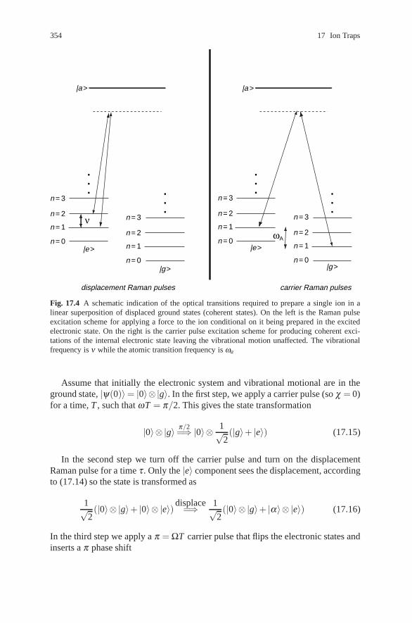
354 17 Ion Traps
.
.
. ...
.
.
. ...
|e >
|g >
n = 0
n = 1
n = 2
n = 3
n = 0
n = 1
n = 2
n = 3
|a > |a >
|e >
|g >
displacement Raman pulses carrier Raman pulses
n = 0
n = 1
n = 2
n = 3
n = 0
n = 1
n = 2
n = 3νωA
Fig. 17.4 A schematic indication of the optical transitions required to prepare a single ion in alinear superposition of displaced ground states (coherent states). On the left is the Raman pulseexcitation scheme for applying a force to the ion conditional on it being prepared in the excitedelectronic state. On the right is the carrier pulse excitation scheme for producing coherent exci-tations of the internal electronic state leaving the vibrational motion unaffected. The vibrationalfrequency is ν while the atomic transition frequency is ωa
Assume that initially the electronic system and vibrational motional are in theground state, |ψ(0)〉= |0〉⊗|g〉. In the first step, we apply a carrier pulse (so χ = 0)for a time, T , such that ωT = π/2. This gives the state transformation
|0〉⊗ |g〉 π/2=⇒ |0〉⊗ 1√
2(|g〉+ |e〉) (17.15)
In the second step we turn off the carrier pulse and turn on the displacementRaman pulse for a time τ . Only the |e〉 component sees the displacement, accordingto (17.14) so the state is transformed as
1√2(|0〉⊗ |g〉+ |0〉⊗ |e〉) displace
=⇒ 1√2(|0〉⊗ |g〉+ |α〉⊗ |e〉) (17.16)
In the third step we apply a π = ΩT carrier pulse that flips the electronic states andinserts a π phase shift

17.3 Novel Quantum States 355
1√2(|0〉⊗ |g〉+ |α〉⊗ |e〉) π=⇒ 1√
2(|α〉⊗ |g〉− |0〉⊗ |e〉) (17.17)
In the fourth step we apply another state selective displacement with a relativephase φ ,
1√2(|α〉⊗ |g〉− |0〉⊗ |e〉) displace
=⇒ 1√2(|α〉⊗ |g〉− |αeiφ〉⊗ |e〉) (17.18)
In the fifth and final step, we apply another π/2 pulse to give
1√2(|α〉⊗ |g〉− |αeiφ〉⊗ |e〉) π/2
=⇒( |α〉− |αeiφ 〉
2
)⊗|g〉+
(|α〉+ |αeiφ 〉2
)⊗|e〉
≡ |α−〉⊗ |g〉+ |α+〉⊗ |e〉 (17.19)
If we now readout the state of the ion, the conditional states are highly non classicalsuperpositions of two different coherent states of vibrational motion,|α±〉 known inquantum optics as cat states.
Fig. 17.5 The probability tofind the ion in the ground stateas a function of the phase ofdisplacements for differentchoices of the magnitude ofdisplacement. From Fig. 4 ofMonroe et al., Science, 272,1135 (1996)
Pg(φ)
0.0
0
0.5
1.0
0.0
0.5
1.0
0.0
0.5
1.0
A
B
C
D
E
0.0
0.5
1.0
0.0
0.5
1.0
φ
α = 6 (theory)
α = 2.97(6)
α = 1.92(4)
α = 1.20(3)
α = 0.84(2)
−π −π/2 π/2 π
356 17 Ion Traps
We thus have correlated different motional states with each of the electronicstates. This kind of entangled state is reminiscent of Schrodinger’s famous thoughtexperiment in which two different metabolic (and thus macroscopic) states of a catare correlated with a two level system in just this way. Indeed if we stopped af-ter the second step the cat state analogy could be sustained with the identification|α〉 → |alive〉 and |0〉 → |dead〉. However pursuing the analogy to the final state atthe end of step 5 produces the rather disturbing prospect (for the cat at least) ofcorrelating different superposition of metabolic states with the internal electronicstates. It is for this reason that superpositions of coherent states are called cat statesin quantum optics.
In the experiment of Monroe at al. [9], the presence of an entangled state ofdifferent coherent states was demonstrated by measuring the electronic state at theend of step 5. Repeated measurements enabled a sampling of the distribution Pg(φ),for different values of φ . This is given by
Pg(φ) = 〈α−|α−〉=
12
[1− e−|α |
2(1−cosφ) cos(|α|2 sinφ
)](17.20)
In Fig. 17.5 we reproduce the results from Monroe et al. [9] comparing the experi-ment with the theoretical prediction in Eq. 17.20. The agreement is remarkable.
17.4 Trapping Multiple Ions
In a linear ion trap such as depicted in Fig. 17.1, multiple ions may be trapped andcooled to the collective ground states of vibrational motion. Each ion has an equilib-rium position, xi, corresponding to a minimum in the total potential comprising thetrap plus Coulomb potential for each ion. These equilibrium points are analogous tothe atomic ions at the lattice points of a crystal, however unlike a crystal they are notequally spaced. In terms of a natural length scale given by the Coulomb potentialfor each ion,
l =(
Z2e2
4πε0Mν2
)1/3
, (17.21)
and a coordinate system in which z = 0 is in the middle of the trapped ions,James [10] has computed the equilibrium positions for different numbers of ionsin a trap, see Fig. 17.6
If we expand the overall potential to second order in the small oscillations, qn(t)(in dimensionless units), around the equilibrium points we obtain a simple coupledoscillator Hamiltonian of the form,
H =1
2M
N
∑n=1
p2m +
Mν2
2
N
∑n,m=1
Anmqnqm (17.22)

17.4 Trapping Multiple Ions 357
Fig. 17.6 The equilibrium positions for varying numbers of ions in the trap in units of the lengthscale given in 17.21. From Fig. 1 James et al. Appl. Phys. B, 66, 181, (1998)
where pn is the canonical momentum to qn. Explicit expressions for the coefficientsAnm are given in [10]. This Hamiltonian represents a linear array of N simple har-monic oscillators with quadratic coupling. We can now make a change of variable tonormal-mode coordinates (sometimes called collective or global coordinates). Thetransformation is chosen to diagonalise the real symmetric N×N matrix with entriesAnm. The eigenvalue equation is
N
∑n=1
Anmβ (p)n = μpβ (p)
m (p = 1, . . . ,N) (17.23)
where the eigenvalues are μp > 0 and the eigenvectors �β (p) are assumed to be num-bered in order of increasing eigenvalue and are normalised so that
N
∑p=1
β (p)n β (p)
m = δnm
N
∑n=1
β (p)n β (q)
n = δpq
For example, when N = 3 the eigenvalues are μ1 = 1,μ2 = 3,μ3 = 29/5. The normalmodes are then given in terms of the small oscillations as
Qp(t) =N
∑m=1
β (p)m qm(t) (17.24)
Note the number of normal modes is equal to the number of ions. Of course we canequally well write the local coordinates qn as
qm(t) =N
∑p=1
β (p)m Qp(t) (17.25)
The first normal mode, Q1 represents the centre of mass mode in which all theions oscillate as if they were train wagons linked together. The second mode Q2 rep-resents a breathing mode in which each ion oscillates with an amplitude proportionalto is displacement form the trap centre. In terms of the normal mode coordinates,Qp and conjugate momenta Pp, the Hamiltonian is

358 17 Ion Traps
H =1
2M
N
∑p=1
P2p +
M2
N
∑p=1
ν2pQ2
p (17.26)
where the frequencies of each of the normal modes is given by
νp = ν√μp (17.27)
This is the Hamiltonian of N independent simple harmonic oscillators. Thus weintroduce raising and lowering operators for each normal mode as
Qp =
√h
2Mνp(bp + b†
p) (17.28)
Pp = −i
√hMνp
2(bp−b†
p) (17.29)
with [bp,b†q] = δpq.
Let us now assume that each ion in the trap can be addressed with a separate laserbeam. For example in a linear ion trap for 40Ca+ built in Innsbruck, the averagespacing for 4 ions was greater than 5μm, which is above the diffraction limit for thelaser beams. This spacing is also sufficient for the fluorescence (at readout) of eachion to be separately imaged.
The interaction picture Hamiltonian describing how the ith ion is coupled to smalloscillations around equilibrium is given by an obvious generalisation of Eq. 17.4
H(i)I = h
Ωi
2
(σ (i)− e−ikL(qi(t)e−i(ωA−ωL)t + h.c
)(17.30)
where we have taken the Rabi frequency for the ith ion to be Ωi and σ (i)± are the
Pauli raising and lowering operators for the ith ion, while qi(t) are local coordinatesof the ith ion. If we now again assume that the Lamb–Dicke parameter for each ionis small, the interaction between the electronic and vibrational degree of freedom is
H(i)I =−ih
kLΩi
2
(σ (i)− qi(t)e−i(ωA−ωL)t −h.c
)(17.31)
This may be written in terms of the global modes as
H(I)I =−ih
ηΩi
2√
N
N
∑p=1
s(p)i
(bpe−iνpt + b†
peiνpt)
e−i(ωA−ωL)tσ (i)− −h.c (17.32)
where s(i)p =√
Nμ−1/4p β (p)
i .We now assume that we can tune the external laser to address only a single
global vibrational mode (a particular normal mode), say the centre of mass mode
at frequency, μ1 = ν and s(1)i = 1 with ωA−ωL = ν . Then we can ignore all the
other modes and approximate the Hamiltonian as
17.5 Ion Trap Quantum Information Processing 359
H(i)I =−ih
ηΩi
2√
N
(σ (i)
+ b1 + σ (i)− b†
1
)(17.33)
This is the Cirac–Zoller Hamiltonian [1] and was used by these authors in a schemefor quantum computing using trapped ions (see below). If there are many ions in thetrap this may not be a good approximation. In that case there are many normal modesand it is difficult to resolve individual normal mode frequencies as they becomevery closely spaced. To some extent this may be mitigated by cooling all the normalmodes to their ground states. Further discussion of the validity of this approximationmay be found in [10] and also [11].
There is an interesting interpretation of the Hamiltonian for local modes, (17.31).Define
σ (i)1 (t) = σ−e−iΔ t + σ+eiΔ t (17.34)
with Δ = ωA−ωL. Now define a quantum field ψ(x,t) = (2Mν/h)1/2qi(t) by re-placing the discrete index, i, with a position variable x = idi where di is the posi-tion of the ith ion form the centre of the trap. This field is a scalar field operatordescribing the small oscillations of the ion at x from equilibrium. The interactionHamiltonian then takes the form
HI = hχψ(x,t)σ1(x,t) (17.35)
which is in the form of local field dipole detector interaction Hamiltonian, withχ = ηΩ/2.
17.5 Ion Trap Quantum Information Processing
In 1995 Cirac and Zoller [1] proposed the first scheme for implementing quan-tum logic gates for trapped ions. In a quantum computer information is stored inthe states of a collection of two level systems, generically referred to as qubits. Inthe Cirac–Zoller (CZ) scheme, the qubits are the two-level electronic states of thetrapped ions. Arbitrary transformations of the state of a single qubit are easily im-plemented by external laser fields. For universal computation we also need to haveaccess to two qubit interactions. However the electronic states of different ions donot interact. CZ proposed to overcome this by using the collective vibrational modeof the ions to implement a virtual interaction between the qubits.
We will discuss a way to implement a particular two qubit interaction, known asa controlled NOT (CNOT) gate which is a universal two-qubit gate. If we denotethe two states of a qubit as |x〉,x = 0,1, the CNOT gate is defined by the unitarytransformation
UCN |x〉⊗ |y〉= |x〉⊗ |x⊕ y〉 (17.36)

360 17 Ion Traps
Fig. 17.7 The electronic levelscheme for each ion in theCNOT gate scheme of Ciracand Zoller
|e> |1>
|0>
where x⊕ y is addition modulo two. In words, the state of the second qubit, calledthe target, is flipped if and only if the state of the first qubit, the control, is |1〉. In allcases the state of the control qubit is unchanged.
In the CZ scheme each ion has a set of internal electronic levels, |0〉, |1〉 and |e〉,depicted in Fig. 17.7. The mapping between physical electronic states and logicalstates is |0〉 ↔ |0〉, |1〉 ↔ |1〉. Note that in addition to the qubit states, there is anadditional auxiliary state, |e〉 which helps implement the degree of control required.We suppose that is possible to direct a laser onto a particular ion inducing elec-tronic transitions in that ion alone. This can couple the qubit state of the ion to itsvibrational degree of freedom. In the Lamb–Dicke limit and for carefully chosendetunings, it is possible to couple a single qubit state to a chosen collective state ofvibrational motion of all the trapped ions. In the CZ scheme the collective vibra-tional modes are all prepared in the ground state by a prior sideband cooling step.
Let us suppose the laser is directed towards the nth ion and tuned to the first redsideband of the collective centre of mass mode described by raising and loweringoperators, a†,a. The Hamiltonian for this is
H = hηΩ
2√
N(a|1〉n〈0|e−iφ + a†|0〉n〈1|eiφ ) (17.37)
If this laser is on for a time T such that ηΩT√
N = kπ ( a kπ-pulse), the unitaryoperator,
Uk,n01 (φ) = exp
[−i
π2
(a|1〉n〈0|e−iφ + a†|0〉n〈1|e−iφ )]
(17.38)
is implemented. This unitary interaction couples the electronic states to the vibra-tional phonon number states |0〉, |1〉;
Uk,n01 (φ)|0〉n|1〉 = cos(kπ/2)|0〉n|1〉− ieiφ sin(kπ/2)|1〉n|0〉 (17.39)
Uk,n01 (φ)|1〉n|0〉 = cos(kπ/2)|1〉n|0〉− ie−iφ sin(kπ/2)|0〉n|1〉 (17.40)
We will also need to implement kπ pulse between the ground state |0〉 and the aux-iliary excited state |e〉. This implements the unitary transformation
Uk,n0e (φ) = exp
[−i
π2
(a|e〉n〈0|e−iφ + a†|0〉n〈e|e−iφ )]
(17.41)
and can be done by changing the polarisation of the exciting laser.We now consider a three pulse sequence: on the mth ion implement U1,m
01 (0),then on the nth ion a 2π pulse between the ground state and the auxillary excitedstate, U2,n
0e (0), finally, again on the m’th ion, U1,m01 (0). The three pulse sequence thus
implements the product unitary, Um,n = U1,m01 (0)U2,n
0e (0)U1,m01 (0). Acting on each of

17.5 Ion Trap Quantum Information Processing 361
the four possible two qubit states of the ions we find that all states remain unchangedexcept when both ions are initially excited;
|1〉m|1〉n→−|1〉m|1〉n (17.42)
This is a two qubit gate known as the CSIGN gate. To use this to implement a CNOTgate we now choose one of the ions to be the control qubit, say mth ion, and first usea laser pulse to put it into a superposition of the logical states, |0〉m + |1〉m. This canbe done by tuning the laser to the carrier frequency so that it is resonant with the|0〉m↔ |1〉m transition, adjusting the phase and pulse area to implement the unitary
Vm = exp[−π
4(|1〉m〈0|−h.c.)
](17.43)
After we implement the V single qubit unitary on the mth ion we implement aCSIGN between the mth ion and the nth ion, target ion. Finally we again act witha V pulse on the mth ion. The net effect is to implement a CNOT gate between themth ion as the control on the nth ion as the target. Clearly the ions do not needto be adjacent. Furthermore we can implement a number of CNOT gates betweendifferent pairs in parallel so long as we can individually resolve the ions with thecontrol lasers. The Cirac–Zoller scheme was first implemented by the Innsbruckgroup led by Blatt in 2003 [12]. They used two 40Ca+ ions held in a linear trap andindividually addressed by focussed laser beams.
Other schemes have been proposed for implementing quantum gates in ion traps.Sørenson and Mølmer [13] developed a scheme which mitigates to some extent thedeleterious effects of noise entering via the vibrational degree of freedom (e.g. patchpotential heating) and implemented by the Wineland group in NIST [14]. A relatedscheme [15] uses far off-resonance optical dipole forces to implement a geomet-ric phase gate, also first implemented by the NIST group [16]. The basic idea of ageometric phase gate is to use a sequence of laser pulse sequences, applied to twoions, that move the vibrational degree of freedom of the ion through a loop in phasespace that depends on the internal states of the two ions. A simple, though imprac-tical, way to achieve this is to use phase space displacements that move around arectangle in phase space, starting at the origin, in a direction that depends on theinternal state of the ion. For example, the unitary operators
Uj(κx) = e−iκx pσz,n/h (17.44)
Uj(κp) = e−iκpxσz,n/h (17.45)
give conditional displacements of the vibrational degree of freedom along the x-axisfor the jth ion in the case of Uj(κx) and along the p-axis in the case of Uj(κp). Ifwe use the commutation relation [x, p] = ih we can show that the following
Uk(κp)Uj(−κx)Uk(−κp)Uj(κx) = eiκxκpσz, jσz,k (17.46)

362 17 Ion Traps
|0>(1)|0>(2) |1>(1)|1>(2) |0>(1)|1>(2) |1>(1)|0>(2)
−χ
−χ
χ
χx
p
Fig. 17.8 The conditional phase space displacements of the vibrational degrees of freedom oftwo ions. Four cases are shown corresponding to the four distinct states of two qubits. The pathfollowed is different for each case but the enclosed area is the same
This is an Ising-like two qubit unitary interaction between the j,kth qubits. Notethat there is no dependance on the vibrational degree of freedom at all. Inspection ofthe various phase space orbits, see Fig. 17.8 indicates why this is called a geometricphase gate. The effective conditional phase between the two qubits is proportionalto the area of the rectangle, χ = κxκp and the sign is given by the sense of rotation. Itis clear that the actual shape of the closed orbit in phase space does not matter: onlythe area and sense of rotation matter. In an experiment the phase space rotations aredone by a time varying driving fields, with both amplitude and phase modulation(see Exercise 17.3). The idea of conditional phase space displacements opens up apath to fast quantum gates for two ions [17].
Exercises
17.1 A laser is tuned to the first read sideband transition for a single two level tran-sition, |g〉 ↔ |e〉, with a spontaneous emission rate of γ. Ignoring all but thespontaneous emission decay channel, the master equation (in the interactionpicture) describing this system is
dρdt
=ηΩ2
[aσ+−a†σ−,ρ ]+ γD [σ−]ρ (17.47)
where η is the Lamb–Dicke parameter, Ω is the Rabi frequency for thetransition and a,a† are the lowering and raising operators for the vibra-tional motion of the ion in the trap. Obtain equations of motion for n =〈a†a〉, 〈a〉, 〈σ±〉, 〈σz〉 by factorising all higher order moments in the equa-tions of motion. Assuming that the spontaneous emission rate is large enoughso that the average polarisation 〈σ±〉 is stationary and the vibrational motionis slaved to the atomic motion, show that the rate of change of n is given by(17.13).
17.2 A simple mode for the heating of a trapped ion due to fluctuation potentialsmay be given in terms of the Hamiltonian
H(t) = hνa†a + hε(t)(a + a†) (17.48)
References 363
where ε(t) is fluctuating force term with the following classical moments
ε = E (ε(t)) = 0
G(τ) = E (ε(t)ε(t + τ)) =D2γ
e−γ|τ|
Show that the heating rate is given by
d〈a†a〉dt
=π2
S(ν) (17.49)
where the noise power spectrum for the fluctuating force is defined by
S(ω) =1
2π
∫ ∞
−∞e−iωtG(τ) (17.50)
17.3 Show that if a harmonic oscillator in its ground state is subjected to a sequenceof displacements in phase space that form a closed loop, the state is returnedto the ground state up to an overall phase proportional to the area of the loop.
References
1. J.I. Cirac, P. Zoller: Phys. Rev. Letts. 74, 4091 (1995)2. H.G. Dehmelt: Bull. Am. Phys. Soc. 20, 60 (1975)3. J.C. Bergquist, R.G. Hulet, W.M. Itano, D.J. Wineland: Phys. Rev. Lett. 57, 1699 (1986):
W. Nagourney, J. Sandberg, H.G. Dehmelt: Phys. Rev. Lett. 56, 2797 (1986); T. Sauter,W. Neuhauser, R. Blatt, P. E. Toschek: Phys. Rev. Lett. 57, 1696 (1986)
4. Ch. Roos, Th. Zeiger, H. Rohde, H.C. Nagerl, J. Eschner, D. Leibfried. F. Schmidt-kaler,R. Blatt, Phys. Rev. Letts., 83, 4713 (1999)
5. D. Leibfried, R. Blatt, C. Monroe, D. Wineland: Rev. Mod. Phys. 75, 281 (2003)6. J.I. Cirac, R. Blatt, P. Zoller, W.D. Philips: Phys. Rev. A 46, 2668 (1992)7. C. Monroe, D.M. Meekhof, B.E. King, S.R. Jefferts, W.M. Itano, D.J. Wineland, P.L. Gould:
Phys. Rev. Lett. 75, 4011 (1995)8. M.J. Gagen, G.J. Milburn: Phys. Rev. A 45, 5228 (1992)9. C. Monroe, D.M. Meekhof, B.E. King, D.J. Wineland: Science, 272, 1131 (1996)
10. D.F.V. James: Appl. Phys. B 66, 181, (1998)11. D.J. Wineland, C. Monroe, W.M. Itano, D. Liebfried, B.E. King, D.M. Meekhof: J. Res. Natl.
Stand. Technol. 103, 259 (1998)12. F. Schmidt-Kaler, H. Haffner, M. Riebe, S. Gulde, G.P.T. Lancaster, T. Deuschle, C. Becher,
C.F. Roos, J. Eschner, R. Blatt: Nature, 422, 408, (2003)13. A. Sørensen, K. Mølmer: Phys. Rev. A 62, 022311 (2000)14. C.A. Sackett, D. Kielpinski, B.E. King, C. Langer, V. Meyer, C.J. Myatt, M. Rowe,
Q.A. Turchette, W.M. Itano, D.J. Wineland, C. Monroe: Nature, 404, 256 (2000)15. G.J. Milburn, S. Schneider, D.F.V. James: Fortschritte der Physik, 48, 801 (2000)16. D. Leibfried, B. De MArco, V. Meyer, D. Lucas, M. Barrett, J. Britton, W.M. Itano,
B. Jelenkovic, C. Langer, T. Rosenband, D.J. Wineland: Nature, 422, 412 (2003)17. J.J. Garcia-Ripoll, P. Zoller, J.I. Cirac: Phys. Rev. Lett. 91, 157901 (2004); L.-M. Duan: Phys.
Rev. Lett. 93, 100502 (2004)

Chapter 18Light Forces
Abstract In recent years it has become possible to manipulate atoms with lightbeams, to trap them and cool them to temperatures of milliKelvin and below. Thefirst proposal of laser cooling by Hansch and Schawlow [1] was based upon Dopplercooling in a two-level atom. Consider an atom irradiated by counterpropagatinglaser beams tuned to the low frequency side of atomic resonance. The beam counter-propagating with the atom will be Doppler shifted towards resonance, thus increas-ing the probability of photon absorption. The beam co-propagating with the atomwill be frequency-shifted away from resonance, so there will be a net absorption ofphotons opposing the motion of the atom. The absorbed photon gives the atom amomentum impulse Δp = hk = h/λ in the direction of the beam. The atom re-emitsa photon by spontaneous emission in a random scattering direction. Thus, the netforce of the time averaged emitted photons is zero. The resultant force due to theabsorption of the photons opposes the atom’s motion. By surrounding the atom withthree pairs of counter-propagating beams along the x, y and z axes, a drag forceopposing the velocity of the atom can be generated. The term “optical molasses”was coined to describe this situation. For two level atoms the minimum temperatureachievable, the so-called Doppler limit, was predicted to be kBT = hγ/2, where γis the atomic decay rate. Optical molasses in sodium was first observed in 1985 byChu et al. [2] with a temperature∼ 240μK, close to the Doppler limit.
In order to trap the cold atoms, techniques including purely optical forces, thedipole trap, or a combination of optical and magnetic forces, the magneto-opticaltrap (MOT), were developed. Experiments performed by W. Phillips [3] and col-leagues cooling sodium atoms in a MOT recorded temperatures considerably lowerthan expected, i.e. ∼ 40μK as opposed to TD ∼ 240μK. The explanation for thelower temperatures observed experimentally was given by Dalibard and Cohen-Tannoudji [4] and Chu [5] and colleagues. They showed that optical pumping be-tween atomic magnetic sublevels could result in lower temperatures (sub-Dopplercooling) with a limit close to the recoil energy,
kBT = hωRec ,
with hωRec = h2k2/2M.
365

366 18 Light Forces
More recently, sub recoil cooling schemes have been proposed and implemented,using, for example, the accumulation of ultracold atoms in dark states, which do notcouple to the light fields provided the atomic kinetic energy is less than the recoilenergy.
In 1997 the Nobel Prize in Physics was awarded to Steven Chu, Claude Cohen-Tannoudji and William Phillips for their work on atom trapping and cooling. Inthis chapter we shall present a theoretical description of light forces on a two levelatoms. We shall follow closely the treatment developed by Gordon and Ashkin [6]and Cohen-Tannoudji [7].
18.1 Radiative Forces in the Semiclassical Limit
We begin with the Hamiltonian for a two–level atom coupled to the electromagneticfield and driven by a near–resonant laser field:
H = HA +HV +HAL +HAV . (18.1)
Here, HA is the atomic Hamiltonian,
HA =�P2
2m+
hωa
2σz (18.2)
with σz = (|e〉〈e|− |g〉〈g|), HV is the Hamiltonian of the (vacuum) radiation field,HAV is the coupling of the atom to this field, and HAL describes the atom–lasercoupling,
HAL(�R) =−�d ·�EL(�R,t) = hΩL(�R)[σ+e−i(ωLt−Φ(�R)) + h.c.
], (18.3)
where σ+ = |e〉〈g| and the rotating wave approximation has been made. The inter-action with the vacuum field is
HAV(�R) = h[σ+Γ(�R)+ σ−Γ†(�R)
], (18.4)
where Γ(�R) is the bath operator for the vacuum defined as
Γ(�R) = ∑k
gkbke−i(ωkt−�k·�R) (18.5)
(see Sect. 10.1).The force acting, �F(�R), on the atom is given by
�F(�R) =−∇HAL(�R)−∇HAV(�R)

18.1 Radiative Forces in the Semiclassical Limit 367
The coupling of the atom to the vacuum radiation field is responsible for spon-taneous emission. This process introduces friction and damping to the system–necessary for Doppler cooling – but it also introduces some of the fluctuations whichlead to momentum diffusion, limiting the final temperatures.
In a classical description the atom has a well–defined position and a well–definedmomentum. For a semiclassical description to be valid, one therefore requires thatthe atomic wave packet be sufficiently well localised in position space and in mo-mentum space.
Denote the spatial and momentum spreads of the atomic wave packet by ΔRand ΔP, which must satisfy (ΔR)(ΔP) ≥ h. The force exerted by the laser on theatom varies on a distance determined by the laser wavelength λL. If the atom isvery well localised on this scale we can neglect the fluctuations of the force due tothe spread in atom positions and simply evaluate the force at the average positionof the wave packet. Furthermore, as atoms moving with different velocities see avarying Doppler shift, the force due to the laser will also fluctuate due to momentumfluctuations. However if the initial momentum fluctuations are small enough we canneglect fluctuations in Doppler shifts and assume all atoms see a single Dopplershift determined by the mean velocity of the atomic wave packet. We are thus led totwo conditions for a semiclassical description to be valid (i) that the position spreadbe small compared to λL,
ΔR� λL ⇔ kLΔR� 1 (18.6)
and(ii) that the velocity spread be small enough that the corresponding spread ofDoppler shifts be negligible compared to the natural linewidth γ ,
kLΔPm� γ . (18.7)
Combining (18.6) and (18.7) with the uncertainty relation gives
hk2L
m� γ or hωrec� hγ . (18.8)
It turns out that this is equivalent to the condition that the timescale for internalatomic evolution (∼ γ−1) is much shorter than the timescale for external evolution[∼ (hk2
L/m)−1], i.e., for damping of the motion.We now denote the mean atomic position and momentum by�r = 〈�R〉 and �p = 〈�P〉.
The semiclassical force is given by
�f =− 〈∇HAL(�r,t)〉|�r=�r0+�v0t . (18.9)
Note that contribution from the atom–vacuum–field coupling term, HAV, vanishes,due to the symmetry of spontaneous emission. Now
−∇HAL(�r,t) =−hσ+exp−iωLt∇[Ω(�r)exp−iΦ(�r)
]+ h.c. , (18.10)

368 18 Light Forces
and we can write
∇[ΩL(�r)exp−iΦ(�r)
]= ΩL(�r)exp−iΦ(�r)
[�α(�r)− i�β(�r)
](18.11)
where
�α(�r) =∇ΩL(�r)ΩL(�r)
, �β (�r) = ∇Φ(�r) . (18.12)
�α(�r) – characterises spatial variation of the Rabi frequency.�β (�r) – characterises spatial variation of the phase.
This gives the following expression for the mean force,
�f (�r,t) = −2Re{〈σ+(t)〉 hΩL(�r)exp−i[ωLt+Φ(�r)]
[�α(�r)− i�β(�r)
]}
= −2hΩL(�r)[u(t)�α(�r)+ v(t)�β(�r)
], (18.13)
where 〈σ+(t)〉= Tr[σ+ρint(t)], with ρint(t) the internal atomic density operator, and
u(t) = Re{〈σ+(t)〉exp−i[ωLt+Φ(�r)]
}(18.14)
v(t) = Im{〈σ+(t)〉exp−i[ωLt+Φ(�r)]
}. (18.15)
The average values of the internal atomic operators are computed from the opticalBloch equations, which, in terms of the variables defined above, take the form
u = −(γ/2)u +(δ + Φ)v
v = −(γ/2)v− (δ + Φ)u−2ΩLw
w = −(γ/2)− γw+ 2ΩLv (18.16)
where w = [〈σ+σ−〉−〈σ−σ+〉]/2 is the inversion, δ = ωL−ωA is the laser–atomdetuning, and
Φ =�v ·∇Φ =�v ·β . (18.17)
18.2 Mean Force for a Two–Level Atom Initially at Rest
Some physical insight into the nature of the forces acting on the atom can be gainedby considering the zero velocity case. Consider a two–level atom initially at rest atthe origin:
�r = 0 , �p = 0 . (18.18)
The steady state solutions of the optical Bloch equations are:

18.2 Mean Force for a Two–Level Atom Initially at Rest 369
uss =δ
2ΩL
s1 + s
(18.19)
vss =γ
4ΩL
s1 + s
(18.20)
wss = − 12(1 + s)
(18.21)
where s is the saturation parameter,
s =2Ω2
L
δ 2 +(γ2/4). (18.22)
Note that the population of the upper state is given by
Pess = wss + 1/2 =
12
s1 + s
. (18.23)
Substituting the steady-state values uss and vss in the expression (18.13) for theforce gives the average force in the case where the internal degrees of freedom havereached their steady state (adiabatic approximation). The mean force �f f is the sumof two contributions proportional to v and u, respectively. These two contributionsare known as the spontaneous force and the dipole force (or dissipative force andreactive force).
The spontaneous force is due to the radiation pressure. It results from the absorp-tion of photons from a traveling wave laser from which the atom receives a transferof momentum. The subsequent spontaneous emission of photons does not contributeto the average force since spontaneous emission occurs with equal probabilities inall directions. The dissipative force is zero for a stationary atom in a standing wavesince absorption of photons from both directions cancel. The spontaneous force isgiven by the component proportional to vss,
�fspon =−2hΩLvss�β . (18.24)
Note that −2ΩLvss = γρess which is simply the mean number of photons sponta-
neously emitted per unit time.For a plane wave,
�EL(�r,t) = �E0 cos(
ωt−�kL ·�R)
(18.25)
The phase of the field is Φ(�r) =−�kL ·�R which gives
β = ∇Φ|�r=0 =−�kL , (18.26)
and the force,

370 18 Light Forces
fspon = hkL
(γ2
) 2Ω2L
δ 2 +γ2
4+ 2Ω2
L
. (18.27)
For low intensity (s � 1) fspon ∝ Ω2L ∼ IL (laser intensity). For high intensity
laser fields fspon→ hkLγ2 , that is the maximum force is limited by the spontaneous
emission rate. The maximum acceleration imparted to the atom by the dissipativeforce is,
�amax =h�kL
mγ2
. (18.28)
While the recoil velocity vrecoil = hkLm due to absorption of a single photon is small
(∼3 cm/sec for sodium, ∼3 mm/sec for cesium), the number of fluorescent cy-cles/sec is high for intense fields. For sodium γ−1 = 1.6× 10⁻⁸ s, which givesamax ∼ 106 m/s2 which is 105 times the acceleration due to gravity.
The dipole force is given by the component proportional to uss:
�fdip =−2hΩLuss�α (18.29)
In a plane travelling wave, �α = 0 as the amplitude is independent of�r and hence�fdip = 0. The dipole force is only nonzero if the laser field is a superposition ofplane waves, e.g., a laser standing wave. The dipole force results from the absorp-tion of a photon with momentum hk from a standing wave and reemission of aphoton in the opposite direction, that is with momentum −k. This results in a totalmomentum gain for the atom 2hk. For a travelling wave laser the dipole force is zerosince photons can only be reemitted into the same direction from which they whereabsorbed.
Using the solution for uss,
�fdip =−hδ∇(Ω2
L)δ 2 +(γ2/4)+ 2Ω2
L
(18.30)
For δ < 0 (ωL < ωA), the dipole force pushes the atom towards regions of higherintensity since sgn{�fdip}= sgn{∇IL} (and vice–versa for δ > 0). For each value ofΩ2
L (with ΩL� γ), �fdip is optimised for δ ∼ΩL, and
(�fdip
)max� h∇(Ω2
L)ΩL
� h∇ΩL (18.31)
Hence, �fdip increases with laser intensity and is not bounded like �fspon so that muchgreater acceleration is possible with the dipole force.
The dipole force can be derived from an effective potential U as
�Fdip =−∇U , (18.32)

18.3 Friction Force for a Moving Atom 371
with
U(�r) =hδ2
ln
[1 +
2Ω2L(�r)
δ 2 +(γ2/4)
]. (18.33)
For δ < 0, a region of maximum intensity appears as an attractive potential wellfor the atom. For a given ΩL, the maximum depth of the potential well occurs for asaturation parameter s� 4 giving
|Umax| � 0.6 |hΩmaxL | . (18.34)
18.3 Friction Force for a Moving Atom
Now suppose that the atom is moving with a velocity�v, such that
�r =�vt (�r = 0 at t = 0) . (18.35)
As previously we assume also that we are in the semiclassical limit so that fluctu-ations in velocity due to momentum dispersion in the wave packet can be ignored.The velocity, �v, is determined by the average momentum of the wave packet. Weassume a laser plane wave with wave vector�kL, so that the Rabi frequency
ΩL(�r =�vt) = Ω0 = constant (18.36)
while
Φ(�r) =−�kL ·�r ⇒ Φ =d�rdt·∇Φ =�v ·∇Φ =−�kL ·�v . (18.37)
Since ΩL and Φ are time independent (and hence the coefficients of the opticalBloch equations are time independent), the steady state solutions are as before (fora stationary atom), but with ωL→ ωL−�kL ·�v, i.e., an atom moving with velocity �v“sees” the laser frequency shifted by the Doppler shift −�kL ·�v. Hence, the force is
�f = h�kLγ2
2Ω20
(δ −�kL ·�v)2 +(γ2/4)+ 2Ω20)
. (18.38)
We assume �kL = −kL�ex and consider motion along the x axis. For δ < 0 (andvx > 0), the force is negative and has a maximum where δ = −kLvx, i.e., wherethe apparent laser frequency ωL + kLvx = ωA (see Fig. 18.1). Near vx = 0, one canmake an expansion in the velocity, writing where the term linear in vx is a frictionforce, since it is proportional to vx. The coefficient of proportionality, α , is calledthe friction coefficient and is derived as
α =−hk2L
s(1 + s)2
(δγ
δ 2 +(γ2/4)
)(18.39)

372 18 Light Forces
2 4 6 8 10
-1
-0.8
-0.6
-0.4
-0.2
kLv0–δ
γ
fx
(b)(a)
x y
z
kLv0
kL
v0
Fig. 18.1 (a) Atom moving with velocity v0 in a laser travelling wave with wave vector �kL.(b) Mean force experienced by the atom versus kLv0 in units of hkLγ
where s = (2Ω20)/[δ 2 +(γ2/4)]. The friction coefficient is optimised for δ = −γ/2
and s = 1 (Ω0 = γ/2), giving
αmax =hk2
L
4, (18.40)
so that the atomic velocity is damped at a rate
αm
=hk2
L
4m=
εrec
2h(18.41)
where εrec is the recoil energy, i.e., the external atomic variables, such as the ve-locity, have a characteristic damping time on the order of h/εrec (typically between1−100 μs� γ−1).
18.3.1 Laser Standing Wave—Doppler Cooling
The interaction with a standing wave can be considered as the interaction with asuperposition of two counter-propagating plane waves with the same amplitude E0.However the force exerted by the two standing waves is not just the sum of theradiation pressures of the two counter-propagating plane waves. Interference termsplay an important role.
We now consider a laser standing wave along the x axis, linearly polarised alongthe z axis, so that
�EL(�r,t) =�εzE0 [cos(ωLt− kLx)+ cos(ωLt + kLx)]= 2�εzE0 cos(kLx)cos(ωLt) (18.42)
The phase of the field is the same everywhere (�β = 0), while the Rabi frequency isposition dependent and can be written
ΩL(x) = 2Ω0 cos(kLx) (18.43)
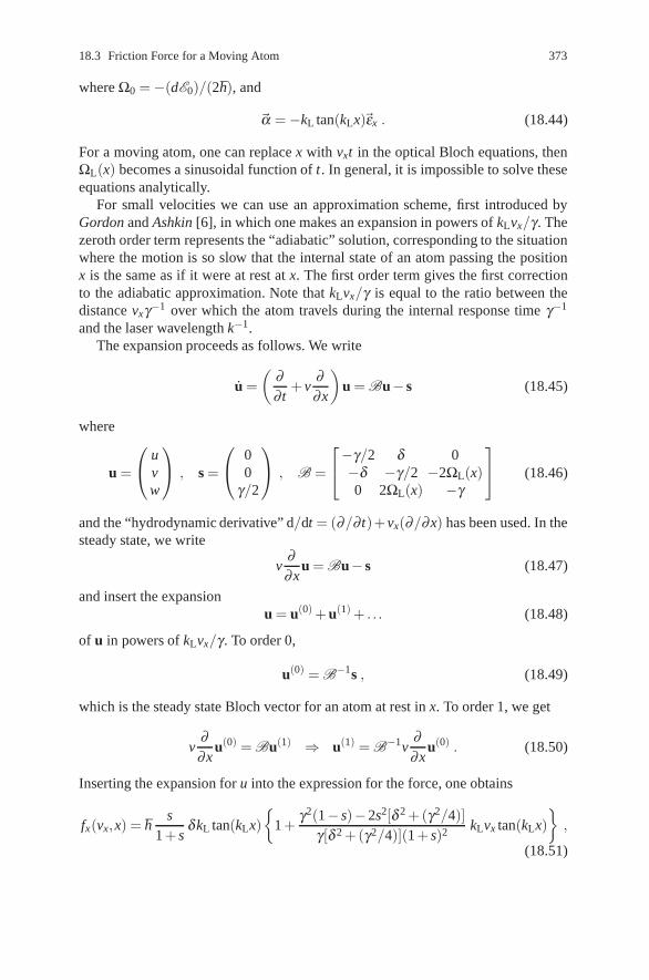
18.3 Friction Force for a Moving Atom 373
where Ω0 =−(dE0)/(2h), and
�α =−kL tan(kLx)�εx . (18.44)
For a moving atom, one can replace x with vxt in the optical Bloch equations, thenΩL(x) becomes a sinusoidal function of t. In general, it is impossible to solve theseequations analytically.
For small velocities we can use an approximation scheme, first introduced byGordon and Ashkin [6], in which one makes an expansion in powers of kLvx/γ . Thezeroth order term represents the “adiabatic” solution, corresponding to the situationwhere the motion is so slow that the internal state of an atom passing the positionx is the same as if it were at rest at x. The first order term gives the first correctionto the adiabatic approximation. Note that kLvx/γ is equal to the ratio between thedistance vxγ−1 over which the atom travels during the internal response time γ−1
and the laser wavelength k−1.The expansion proceeds as follows. We write
u =(
∂∂ t
+ v∂∂x
)u = Bu− s (18.45)
where
u =
⎛⎝ u
vw
⎞⎠ , s =
⎛⎝ 0
0γ/2
⎞⎠ , B =
⎡⎣−γ/2 δ 0−δ −γ/2 −2ΩL(x)0 2ΩL(x) −γ
⎤⎦ (18.46)
and the “hydrodynamic derivative” d/dt = (∂/∂ t)+vx(∂/∂x) has been used. In thesteady state, we write
v∂∂x
u = Bu− s (18.47)
and insert the expansionu = u(0) + u(1) + . . . (18.48)
of u in powers of kLvx/γ . To order 0,
u(0) = B−1s , (18.49)
which is the steady state Bloch vector for an atom at rest in x. To order 1, we get
v∂∂x
u(0) = Bu(1) ⇒ u(1) = B−1v∂∂x
u(0) . (18.50)
Inserting the expansion for u into the expression for the force, one obtains
fx(vx,x) = hs
1 + sδkL tan(kLx)
{1 +
γ2(1− s)−2s2[δ 2 +(γ2/4)]γ[δ 2 +(γ2/4)](1 + s)2 kLvx tan(kLx)
},
(18.51)

374 18 Light Forces
where
s =8Ω2
0 cos2(kLx)δ 2 +(γ2/4)
. (18.52)
For weak intensities, the interference effects average to zero over a wavelength,hence the friction force averaged over a wavelength coincides with the sum of thetwo friction forces exerted by the two counterpropagating plane waves. In particular,
f =−αv with α =−4hk2LΩ2
0δγ
[δ 2 +(γ2/4)]2. (18.53)
Hence, because of the Doppler effect, for δ < 0 the atom gets closer to resonancewith the wave opposing its motion and further away from resonance with the otherwave, so that the two forces exerted by the two waves become unbalanced andthe net force opposes the motion of the atom. This is the mechanism for Dopplercooling.
18.4 Dressed State Description of the Dipole Force
If the Rabi frequency is large compared to the spontaneous emission rate the dressedatom picture provides an intuitive interpretation. We may write the interactionHamiltonian for a two level atom, with frequency ωa, interacting with a single modestanding wave laser field with frequency ΩL = ωa + Δ
HI(x) =hΔ2
σz + hg(x)(aσ+ + a†σ−
), (18.54)
where g(x) = g f (x) is the spatially dependent vacuum Rabi frequency, σ+ = σ†− =
|e〉〈g| and a,a† are the annihilation and creation operators for the field. The dressedstates (see section 10.2) for this interaction are:
|n,+〉 = sinθn(x)|n,e〉+ cosθn(x)|n + 1,g〉 (18.55)
|n,−〉 = cosθn(x)|n,e〉− sinθn(x)|n + 1,g〉 (18.56)
where |n,e〉= |n〉⊗|e〉, |n,g〉= |n〉⊗|g〉with |n〉 a photon number eigenstate. Thecoefficients are given by
cos2θn(x) = − Δ/2Ωn(x)
, (18.57)
sin2θn(x) =g(x)
Ωn(x), (18.58)
and Ωn(x) =√
g2(x)(n + 1)+ Δ2/4 is the effective Rabi frequency. The correspond-ing energy levels are Un,±(x) =±hΩn(x). This is a generalisation of the dressed state

18.4 Dressed State Description of the Dipole Force 375
picture discussed in Sect. 10.2. since the expansion coefficients are now position de-pendent. The dressed states form doublets separated the photon energy hωL.
Typically the optical field is well approximated by a coherent state of large ampli-tude. The Poisson nature of the photon number distribution in such a state enables usto replace Ωn(x) by its average value Ω(x) =
√g2I(x)+ Δ2/4 where I(x) = f 2(x)n
and n is the average photon number is the field. Thus I(x) is the spatially varyingintensity of the field.
The variation in x of the energies of the dressed states are shown in Fig. 18.2for two manifolds ε(N) and ε(N−1). The manifolds are connected by spontaneousemission. Outside the laser beam the energy levels of the dressed states tend to theuncoupled states and are separated by the detuning Δ. Within the laser beam I(x) isnonzero and the splitting
hΩ(x) = h√
4g2I(x)+ Δ2 (18.59)
between the two dressed levels of the same manifold increases with increasing val-ues of I(x).
We shall now use this dressed state picture to provide a physical description of thedipole force. Initially we shall neglect spontaneous emission. We assume the systemis either in state |n,+〉 or |n,−〉 and satisfies the semiclassical limit (7). Assuming theatom velocity is sufficiently slow so that nonadiabatic transitions from one level toanother can be neglected, the system will follow adiabatically the level |n,+〉 or |n,−〉in which it is found initially. The energy curves in Fig. 18.2 are then potential energylevel curves Ve,n(x) and Vg,n(x). The dressed atom therefore experiences a force
Fg =−∇Vg,n(x) =− h2
∇Ω(x) , (18.60)
if it is in level |g〉 and a force
Fe =−∇Ve,n(x) =h2
∇Ω(x) =−Fg, (18.61)
if it is in level |e〉.
Fig. 18.2 The dependance ofthe dressed state energy levelson position due to a spatiallyvarying intensity, a Gaussianbeam profile
hδ-4 -2 2 4 x
|g,n+1>
|e,n>
|n,+>
|n,–>

376 18 Light Forces
Fig. 18.3 A slow movingatom in a standing waveis cooled by spontaneousemission: Sisyphus cooling
|n + 1,+>
|n + 1,–>
|n, +>
|n, –>
|n – 1, +>
|n – 1,–>
This dependence of the force on the internal state is very similar to the Stern–Gerlach effect that occurs for a spin 1
2 particle in an inhomogeneous magnetic field.This effect is known as the optical Stern–Gerlach effect will be described in moredetail in Sect. 18.6. It also provides a mechanism for atom mirrors where atoms inone of the dressed states are repelled by a light field.
Spontaneous emission causes the dressed atom to make a transition to a lowermanifold. In doing so it may change the type of state it is in e.g. a transition|g,n+1 >→ |g,n〉 by emitting a photon. This causes the sign of the force to changeabruptly. The time intervals τ1 and τ2 spent in the different dressed levels betweentwo successive quantum jumps are Poisson random variables. This gives rise to thefluctuations in the dipole force.
The mean dipole force in the steady state is given by the mean of the forces F1
and F2 weighted by the proportion of time spent in the type 1 and 2 levels, whichare simply the steady state populations of the dressed levels π1 and π2. Thus
⟨Fdip
⟩= F1π1 + F2π2 =− h2
2∇Ω(x)(π1−π2) . (18.62)
This corresponds to the expression derived earlier.The dressed state picture gives a clear illustration of the mechanism for cooling
a moving atom in a strong standing wave, known as Sisyphus cooling. In this caseI(x) = I0 sin2(kLx). Figure 18.3 represents the dressed states for a positive detuning(blue detuning). The dressed states are linear combinations of ground and excitedstates, the weighting of which varies sinusoidally in space. If we follow an atomstarting at the node of a standing wave in level |g,n + 1〉, it climbs up the lightgradient until it reaches the top (antinode) where its decay rate is a maximum as themixed state has a significant excited state component. It may then jump into level|g,n + 1〉 which does not effect its mechanical motion or jump into level |e,n〉 inwhich case the atom is again in a valley. It now must climb against the gradient toreach the top where it will decay by spontaneous emission again. The mechanismhas been named Sisyphus cooling by analogy with the story from Greek mythology.

18.5 Atomic Diffraction by a Standing Wave 377
Between two spontaneous emissions, the total energy (kinetic plus potential) ofthe atom is conserved. When the atom climbs up hill, its kinetic energy is trans-formed into potential energy by stimulated emission processes which redistributephotons between the two counterpropagating waves at rate Ω . Atomic momen-tum is therefore transferred to laser photons. The total atomic energy is then dis-sipated by spontaneous emission which carries away part of the atomic potentialenergy. The force reaches its maximum value for velocities such that the atom trav-els over a distance of the order of a wavelength between two spontaneous emissions(kLv0 ∼ γ). The magnitude of this friction force is directly related to the modulateddepth (Ω) of the dressed energy levels and hence increases indefinitely with laserintensity.
18.5 Atomic Diffraction by a Standing Wave
We shall consider the deflection of a beam of two-level atoms by a classical standingwave light field in a cavity. The atomic beam is normally incident on the standingwave and experiences an exchange of momentum with the photons in the light wave.We shall assume that the frequency of the light field is well detuned from the atomicresonance so that we may neglect spontaneous emission.
The Hamiltonian describing the interaction is
H = �ω0
2σz +
p2
2m+�Ω(σ−e−iωt + σ+eiωt)coskx , (18.63)
where p is the centre of mass momentum of the atom along the transverse (x direc-tion), m is the atomic mass, σz and σ± are the pseudo spin operators for the atom,ω0 and ω are the atomic and field frequencies, k = ω/c is the wave number of thestanding wave, and Ω = με0/� the Rabi frequency with μ being the dipole momentand ε0 the maximum field amplitude. We shall assume that the interaction time issufficiently small that the transverse kinetic energy absorbed by the atom during theinteraction can be neglected. This is known as the Raman–Nath regime and requirest < 2π/ωr, where the recoil energy is �ωr = (2r�k)2/2m where r is an integer. Thisis equivalent to neglecting the term p2/2m in the Hamiltonian.
Transforming to the interaction picture with H0 = �ωσz the Hamiltonian maybe written in the form
H = �δω2
σz + 2�Ωσx coskx , (18.64)
where δω = ωa−ω and 2σx = σ+ + σ−. This Hamiltonian may be diagonalisedand written in the form
H = V (x)[cosθ (x)σz + sinθ (x)σx] (18.65)
where
378 18 Light Forces
V (x) = �
√(δω)2 +(2Ωcoskx)2,
cosθ (x) =δω√
(δω)2 +(2Ωcoskx)2,
sinθ (x) =2Ωcoskx√
(δω)2 +(2Ωcoskx)2.
In the limit of large detuning (δω � 2Ωcoskx),
cosθ ≈ 1, and sinθ ≈ 0,
so that
V (x)≈ �δω(
1 +2Ω2 cos2 kx
δω2
). (18.66)
This leads to the effective Hamiltonian
Heff = �δω2
σz +(
2�Ω2 cos2 kxδω
)σz . (18.67)
The atomic state vector in the coordinate representation may be written as
〈x|ψ(t)〉= a(x,t)|a〉+ b(x,t)|b〉 , (18.68)
where |a〉 and |b〉 are the upper and lower atomic states, and a(x,t)(b(x,t)) are theprobability amplitudes for the atom to be in the upper (lower) state at the transversecoordinate x at time t.
We assume that the atoms are initially in their ground state with a Gaussian wave-function
a(ξ ,0) = 0,
b(ξ ,0) = (πσ2)−1/4 exp
(− ξ 2
2σ2
), (18.69)
where ξ = kx and σ is proportional to the r.m.s. transverse position spread of theinput beam. This may be written as
b(ξ ,0) =
(2σ2
η
π
)1/4
exp[−(σηξ )2] , (18.70)
where ση is the r.m.s. transverse momentum spread of the input beam scaled to thephoton momentum �k(η = p/�k). The Schrodinger equation in the large detuninglimit is
∂∂τ
(ab
)=
(−iΔ− i cos2 ξ
2Δ 0
0 iΔ + i cos2 ξ2Δ
)(ab
)(18.71)

18.5 Atomic Diffraction by a Standing Wave 379
where τ = Ωt and Δ = δω/2Ω. We shall assume that the atom interacts with a fieldof constant amplitude for a time τ . The Rabi frequency is Ω.
The solution for b(ε,τ) may be written in the form [8]
b(ξ ,τ) = exp
[i
(Δ +
14Δ
)τ] ∞
∑n=−∞
inJn
( τ4Δ
)exp(2inξ )b(ξ ,0) . (18.72)
Taking the Fourier transform of this relationship shows the effect in momentumspace is a convolution
b(η ,τ) = exp
[i
(Δ +
14Δ
)τ] ∞
∑n=−∞
inJn
( τ4Δ
)δ (η−2n)∗ b(η ,0)
= exp
[i
(Δ +
14Δ
)τ] ∞
∑n=−∞
inJn
( τ4Δ
)b(η−2n,0) (18.73)
where b denotes the Fourier transform of b.The scattered ground state wavefunction is a superposition of Gaussian modu-
lated plane waves with momenta p = 2n�k. The momentum transferred from thefield to the atom is in even multiplies of �k corresponding to the absorption of aphoton from the (+k) component, followed by induced emission into the (−k) com-ponent of the standing wave. The final output momentum probability distributionis composed of a comb of images of the initial momentum distribution. In order toresolve these peaks it is necessary to have a narrow initial momentum spread suchthat Δp� 2�k or ση � 1. The output momentum distribution is shown in Fig. 18.4for ση = 0.1, where the propagation time after the interaction is assumed short sothat further spreading has been neglected. The above result holds for large atomicdetuning. For smaller atomic detunings spontaneous emission becomes important.Since the recoil imparted to an atom by a spontaneously emitted photon occurs in arandom direction, exchanges of momentum in non-integral multiplies of �k may oc-cur and the diffractive peaks will be smeared out. That is, as the laser is tuned closer
Fig. 18.4 Output momen-tum distribution for atomsscattered from a standingoptical wave in the Kapitza-Dirac regime in the largedetuning limit. Initial RMSmomentum uncertainty isση = 0.1 (units of �k) and thenormalised interaction timeτ/Δ = 10

380 18 Light Forces
Fig. 18.5 Output momentum distribution for atoms scattered from a standing optical wave. Com-parison of experimental data [20] (−) and theoretical predictions [21] (−−−) for (a) Δ = 0,(b) Δ = 0.6, (c) Δ = 1.2 (from [10])

18.6 Optical Stern–Gerlach Effect 381
to the atomic resonance one moves from the diffractive to the diffusive regime. Thetransition from the diffractive to the diffusive regime has been demonstrated in anexperiment by Gould et al. [11]. A fit to their data using a calculation which in-cludes spontaneous emission has been given by Tan and Walls [10] and is shown inFig. 18.5.
18.6 Optical Stern–Gerlach Effect
In the previous section, we discussed the diffraction of atoms in their ground statefrom a standing wave light field. In order to resolve the diffraction peaks in themomentum distribution it was necessary that the initial atomic spatial wave packetbe larger than a wavelength. In this regime, the momentum transfer is symmetricalabout Δp = 0 and is the same for input atoms in either the ground or excited states.As the spatial extent of the input wave packet is reduced to a fraction of the opticalwavelength, the momentum transfer becomes asymmetrical and dependent upon theinitial atomic state. Figure 18.6 shows the outgoing probability density of the atomicmomentum for an initial atomic beam width σ = 0.3. The solid curve is for atomsin the ground state while the dotted curve is for the excited state.
In the limit when the spatial extent of the input wave packet is very small com-pared to the optical wavelength, an input beam is split into two beams dependingon its atomic state. This is called the optical Stern–Gerlach limit in which the atominteracts with only a small part of the light wave (ΔxIN � 1/k) and the individualphoton exchanges are not resolvable (Δp� �k). In the large-detuning limit the mo-mentum transfer, which can be many times the photon momentum, depends on theintensity gradient of the optical field. An experimental demonstration of the opticalStern–Gerlach effect has been given by Sleator et al. [12] using a beam of metastableHe atoms (Fig. 18.7).
Fig. 18.6 Output momentumdistribution for atoms scat-tered from a standing opticalwave in the Stern-Gerlachregime. Initial rms momentumuncertainty is ση = 2.4 (unitsof �k). The atomic beam isincident midway between anode and an antinode and thenormalised interaction timeτ/Δ = 20. (a) solid curve,ground state atoms, (b) dottedcurve, excited state atoms
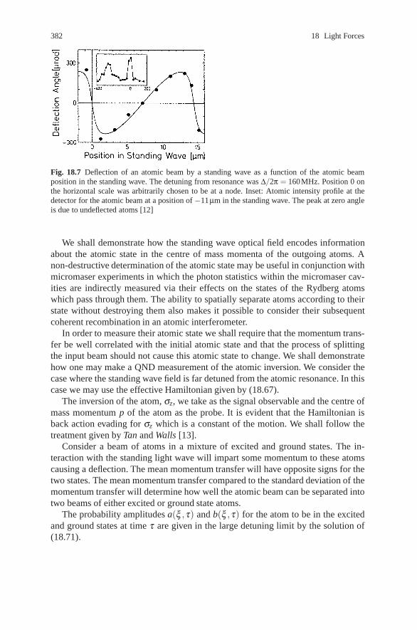
382 18 Light Forces
Fig. 18.7 Deflection of an atomic beam by a standing wave as a function of the atomic beamposition in the standing wave. The detuning from resonance was Δ/2π = 160MHz. Position 0 onthe horizontal scale was arbitrarily chosen to be at a node. Inset: Atomic intensity profile at thedetector for the atomic beam at a position of −11μm in the standing wave. The peak at zero angleis due to undeflected atoms [12]
We shall demonstrate how the standing wave optical field encodes informationabout the atomic state in the centre of mass momenta of the outgoing atoms. Anon-destructive determination of the atomic state may be useful in conjunction withmicromaser experiments in which the photon statistics within the micromaser cav-ities are indirectly measured via their effects on the states of the Rydberg atomswhich pass through them. The ability to spatially separate atoms according to theirstate without destroying them also makes it possible to consider their subsequentcoherent recombination in an atomic interferometer.
In order to measure their atomic state we shall require that the momentum trans-fer be well correlated with the initial atomic state and that the process of splittingthe input beam should not cause this atomic state to change. We shall demonstratehow one may make a QND measurement of the atomic inversion. We consider thecase where the standing wave field is far detuned from the atomic resonance. In thiscase we may use the effective Hamiltonian given by (18.67).
The inversion of the atom, σz, we take as the signal observable and the centre ofmass momentum p of the atom as the probe. It is evident that the Hamiltonian isback action evading for σz which is a constant of the motion. We shall follow thetreatment given by Tan and Walls [13].
Consider a beam of atoms in a mixture of excited and ground states. The in-teraction with the standing light wave will impart some momentum to these atomscausing a deflection. The mean momentum transfer will have opposite signs for thetwo states. The mean momentum transfer compared to the standard deviation of themomentum transfer will determine how well the atomic beam can be separated intotwo beams of either excited or ground state atoms.
The probability amplitudes a(ξ ,τ) and b(ξ ,τ) for the atom to be in the excitedand ground states at time τ are given in the large detuning limit by the solution of(18.71).

18.6 Optical Stern–Gerlach Effect 383
After passage through the field, the mean momentum transfer to this beam isgiven by
〈ηOUT〉=∫ ∞
−∞a(ξ ,τ)∗
(−i∂∂ξ
)a(ξ ,τ)dξ +
∫ ∞
−∞b(ξ ,τ)∗
(−i∂∂ξ
)b(ξ ,τ)dξ
(18.74)where η = p/�k is a normalised momentum. Similarly the mean squared momen-tum transfer is
σ2η = 〈ηOUT2〉=
∫ ∞
−∞a∗(ξ ,τ)
(−∂ 2
∂ξ 2
)a(ξ ,τ)dξ
+∫
b∗(ξ ,τ)(−∂ 2
∂ξ 2
)b(ξ ,τ)dξ . (18.75)
In the large detuning limit we find for a Gaussian beam with width σ centred at ξ0
〈ηOUT± 〉=± τ
2Δe−σ 2
sin(2ξ0) (18.76)
〈ηOUT2
± 〉= σ2η =
12σ2 +
τ2
8Δ2 [1−2e−2σ 2sin2(2ξ0)− e−4σ 2
cos(4ξ0)] (18.77)
where the + sign is for initial state |e〉 and the − sign for initial state |g〉. InFig. 18.8 we plot these quantities as a function of the width of the atomic beamσ for τ/Δ = 20. The mean momentum transfer depends on the gradient of the inten-sity of the light field where the atom crosses and so the atomic beam must be narrow
Fig. 18.8 Mean (solid curve) and standard deviation (dashed curve) of the atomic momentumplotted against the normalised width of the atomic beam. The atomic beam is incident midwaybetween a node and an antinode and the normalised interaction time τ/Δ = 20 (from [13])

384 18 Light Forces
in order for the momentum transfer to be well defined. As the width of the atomicbeam increases, different portions of the beam are deflected differently, reducing themean momentum transfer. The variance of the output momentum arises from twoeffects: The term involving (2σ2)−1 represents the original momentum uncertaintyof the input beam, which increases rapidly as σ is reduced. If, however, σ is in-creased so that it covers a significant portion of an optical wavelength, the variationin momentum imparted to different parts of the beam again increases the variance.Consequently there is a minimum in the standard deviation, as seen in Fig. 18.8. Thecondition for a good measurement is that the mean momentum transfer to the beamprepared in an eigenstate is larger than the spread of the outgoing momentum. FromFig. 18.8 it is clear that there is an optimal width of the input beam which gives thebest quality of measurement. This optimum width depends on the interaction timesince the mean momentum transfer rises with τ/Δ, and for larger interaction timesthis will exceed the intrinsic momentum uncertainty for a narrower initial beam.We may use the QND correlation coefficient introduced in Chap. 14 to evaluate thequality of the measurement. In this case the signal is the atomic inversion σz and theprobe is the centre-of-mass momentum η of the atom.
These correlation coefficients depend on expectation values which have to betaken over some initial state. We choose the state which is a statistical mixture ofground and excited states with equal probability. In the large detuning limit themeasurement correlation may be written as
C2AIN
s AOUTP
=|〈ηOUTσ IN
z 〉|2〈ηOUT2〉〈σ IN2
z 〉
=| 12 [〈ηOUT
+ 〉( 12 )−〈ηOUT− 〉(−1
2 )]|212(〈ηOUT2
+ 〉+ 〈ηOUT2
− 〉) 12 [( 1
2 )2 +(−12 )2]
, (18.78)
from (18.76 and 18.77) this may be written as
C2AIN
s AOUTP
=2σ2τ2e−2σ 2
sin2(2ξ0)4Δ2 + σ2τ2[1− e−4σ 2 cos(4ξ0)]
. (18.79)
The state preparation correlation C2AIN
s AOUTP
has an identical expression. In the large
detuning limit an atom prepared in an eigenstate of σz remains in an eigenstate ofσz. Consequently, the non-demolition correlation
C2AIN
s AOUTs
= 1 . (18.80)
In Fig. 18.9 we plot C2AIN
s AOUTP
as a function of the width of the atomic beam σ for
a range of different interaction times τ/Δ = 2, 5, 10, 20, 50.The position of the beam centre is ξ0 = π/4 corresponding to the point midway
between a node and antinode where the intensity gradient is greatest. We see thatfor sufficiently large interaction times and an atomic beam of optimal width the

18.7 Quantum Chaos 385
Fig. 18.9 Measurement correlation coefficient squared plotted against the normalised width of theatomic beam for τ/Δ = (a) 2, (b) 5, (c) 10, (d) 20, (e) 50 (from [13])
measurement correlation may approach unity. Thus the deflection of an atomic beamby a standing wave field may be used to give a good QND measurement of theatomic inversion σz in the detuning limit. For smaller detuning a QND measurementof an operator dxσ x +dyσy +dzσ z can be made. For example, for zero detuning theappropriate QND observable is the atomic polarisation σx.
18.7 Quantum Chaos
A cold atom moving in a well detuned laser field sees a dipole potential that hasthe same spatial dependence as the field intensity. These potentials are usually nonlinear and anharmonic. They thus provide an ideal means to investigate anharmonicquantum non linear dynamics. Given the ease with which the optical field can bemodulated in time, we also have the possibility of investigating non adiabatic dy-namics of time dependent potentials and quantum chaos.
We can describe both spatial and temporal modulation through the Rabi fre-quency Ω(x,t). As we have seen a two-level atom moving in one dimension (the x-direction) in an off-resonant field can be well described by the effective Hamiltonian
Heff =p2
x
2m+|Ω(x,t)|2
2Δσz (18.81)
where Δ = ωL−ωa. We will typically be concerned with a standing wave laser fieldwith wave vector k, with modulated intensity. In that case
386 18 Light Forces
Ω(x,t) = Ω[1−2ε cos(ωτ)]sin(kx) (18.82)
Following [14] we introduce dimensionless variables for convenience:
k =4hk2
mω(18.83)
κ =hk2Ω2
2mω2Δ(18.84)
t = ωτ (18.85)
q = 2kx (18.86)
p =2kpx
mω(18.87)
Noting that the commutation relation for the dimensionless position and momentumis
[q, p] = ik (18.88)
we see that k has the interpretation of a dimensionless Planck’s constant.We first consider the case of a time independent standing wave. In this case the
Hamiltonian in dimensionless variables is
H =p2
2−κ cosq (18.89)
This is a standard problem in classical nonlinear dynamics and is fully integrable bya canonical transformation to action-angle variables. If at time t = 0 the atom hasinitial conditions (q(t = 0), p(t = 0)) = (q0, p0) it will move in the phase space soas to conserve energy so it must remain on the curve E = p(t)2/2−κ cos(q(t)) =p2
0/2−κ cos(q0). The motion is periodic if the initial energy is such that−κ < E <0, in which case the atom remains localised in one well. For E > κ the motion is un-bounded. The curve E = 0 is called the spearatrix. The frequency of the oscillatorymotion depends on energy, and tends to zero as the initial energy approaches zeroon the separatrix. This is shown in Fig. 18.10.
The nonlinear dependance of oscillator frequency on energy is important whenwe add a periodic temporal modulation to the potential. For a simple harmonic oscil-lator, resonance is only possible at one frequency and this does not depend on initialconditions. For a non linear oscillator this is no longer the case and a complex hier-archy of resonances is possible leading to chaos. In fact, periodically driven systemswith a nonlinear potential is generically chaotic even in one dimension. Consider thecase of an atom in a standing wave with modulated amplitude. The Hamiltonian is
H(t) =p2
2−κ(1−2ε cost)cosq (18.90)
As the Hamiltonian is periodic in time, the most appropriate way to describe thedynamics is in terms of a Poincare section with respect to time. This means that we
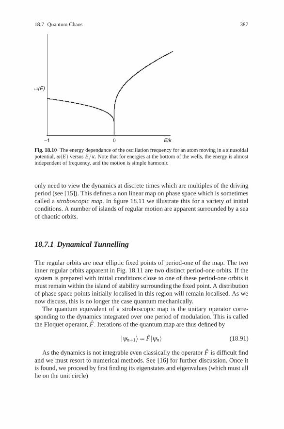
18.7 Quantum Chaos 387
Fig. 18.10 The energy dependance of the oscillation frequency for an atom moving in a sinusoidalpotential, ω(E) versus E/κ . Note that for energies at the bottom of the wells, the energy is almostindependent of frequency, and the motion is simple harmonic
only need to view the dynamics at discrete times which are multiples of the drivingperiod (see [15]). This defines a non linear map on phase space which is sometimescalled a stroboscopic map. In figure 18.11 we illustrate this for a variety of initialconditions. A number of islands of regular motion are apparent surrounded by a seaof chaotic orbits.
18.7.1 Dynamical Tunnelling
The regular orbits are near elliptic fixed points of period-one of the map. The twoinner regular orbits apparent in Fig. 18.11 are two distinct period-one orbits. If thesystem is prepared with initial conditions close to one of these period-one orbits itmust remain within the island of stability surrounding the fixed point. A distributionof phase space points initially localised in this region will remain localised. As wenow discuss, this is no longer the case quantum mechanically.
The quantum equivalent of a stroboscopic map is the unitary operator corre-sponding to the dynamics integrated over one period of modulation. This is calledthe Floquet operator, F . Iterations of the quantum map are thus defined by
|ψn+1〉= F |ψn〉 (18.91)
As the dynamics is not integrable even classically the operator F is difficult findand we must resort to numerical methods. See [16] for further discussion. Once itis found, we proceed by first finding its eigenstates and eigenvalues (which must alllie on the unit circle)

388 18 Light Forces
Fig. 18.11 The classicalphase space orbits for thestroboscopic map with avariety of initial conditions.The modulation strength isε = 0.3
F |φα〉= eiφα |φα〉 (18.92)
It is a remarkable fact that the eigenstates can often be put in one to one correspon-dence with particular orbits of the classical map, using a phase space representationsuch as the Q-function. For example there are pair of nearly degenerate eigenstatesassociated with the period one fixed points near the origin in Fig. 18.11. Given thesolution to the eigenvalue problem the iteration of a given initial state is found byexpanding the state over the Floquet eigenstates, |ψ0〉= ∑α cα |φα〉
|ψn〉= ∑α
cα einφα |φα〉 (18.93)
We now take the initial state to be well localised inside the island of stabilitysurrounding one of the period one orbits. We iterate the state and at each iterationstep calculate the average and variance of the position and momentum. The resultsare plotted in Fig. 18.12. We see a very different situation to what would be expectedclassically (also shown in the figure). The quantum state does not remain localisednear the period one fixed point at which it started. Rather it appears to tunnel acrossclassically forbidden regions of phase space to the symmetric partner of the fixed
s
(a) (b)
200
–1
V (p
)<
p>
V(p
)<
p>
01
–10
1
Strobe number n
400 600 800 1000 200
Strobe number n
400 600 800 1000
Fig. 18.12 The average and variance of position and momentum for an initial classical distribution(a) localised near a period one fixed point and (b) an initial quantum state localised near a periodone fixed point. The quantum system demonstrates tunneling form one period one fixed point toanother

18.7 Quantum Chaos 389
point. This is called dynamical tunneling [17]. Dynamical tunneling was observedby Hensinger et al. [18] using a Bose Einstein condensate to prepare the initiallocalised state in phase space.
18.7.2 Dynamical Localisation
More complicated anharmonic modulation of the optical dipole potential can beeasily implemented. An extreme case corresponds to a kicked system in which thestanding wave is pulsed on and off very quickly compared to the period of freedynamics between pulses. In the limit of infinitely short pulses we obtain the deltakicked rotor described by the Hamiltonian
H(t) =p2
2−κ cosq∑
nδ (t−n) (18.94)
This is a well studied system that classically is described by a stroboscopic mapthat is an example of the standard map. If the kicking strength, κ , is sufficientlylarge the phase space is dominated by large sea of chaotic orbits. In this regionan initial well localised distribution of points spreads very rapidly in position butonly slowly diffuses in momentum. In fact to a very good approximation the spreadin momentum is indeed described by a diffusion process with diffusion constantproportional to κ . See [19] for further detail.
The quantum description of this system gives a very different result. An initialstate well localised in momentum will follow the classical diffusion until a timeknow as the break time. At that time the diffusion in momentum will cease and themomentum variance saturates. This is illustrated in Fig. 18.13. Dynamical localisa-tion using laser cooled atoms was first observed by Raizen’s group in 1995 [20].
Fig. 18.13 Classical (dashed)and quantum (solid) of theaverage momentum squaredversus kick number. In thisexample k = 0.24,κ = 1.2
0 50 100 150 200time
0
20
40
60
<p(
t)2 >
classical
quantum

390 18 Light Forces
18.8 The Effect of Spontaneous Emission
In this section we give a brief presentation of the effect of spontaneous emissionon the nonlinear quantum dynamics of atoms. Even in a far detuned optical dipolepotential there is a non zero probability that the atom will be excited. In that case itsuffers a recoil induced momentum kick. Once in the excited state it can relax to theground state by either stimulated emission or spontaneous emission. The best way todeal with the stochastic momentum kicks resulting from absorption, or stimulatedand spontaneous emission is via the stochastic Schrodinger equation discussed inChap. 6.
We will follow the approach of Dyrting [21]. The coherent coupling betweenthe internal and center-of-mass variables is through the position dependent Rabifrequency. We can write the Rabi frequency in the general form
Ω(x) = Ω f (kx,t) . (18.95)
k = c/ωL is called the wavenumber and ωL is the frequency of the laser. Ω is ameasure of the intensity of the field and without loss of generality it can be chosento be real and may be explicitly time dependent. The quantum mechanical atomcan be described by its internal state |σ〉, where σ represents either g or e, and acentre-of-mass state |ψ〉.
The master equation for a two-level atom interacting with the field includingspontaneous emission is
dRdτ
=− ih
[H, R
]− γL R . (18.96)
The Hamiltonian H generates the coherent dynamics for the center-of-mass and in-ternal states of the atom. The superoperator L describes incoherent evolution dueto coupling with the vacuum field modes at a rate γ . The effect of a spontaneousemission causes the atom to make a transition from its internal excited state to itsground state, and the spontaneously emitted photon changes its center-of-mass mo-mentum by an amount hkn. The direction of the emitted photon n is random and hasthe distribution function
φ(n) =3
8π
(1− (d ·n)2
d ·d
). (18.97)
L is given by
L R =12
(σ†σ R+ Rσ†σ −2σN Rσ†) , (18.98)
and N is the superoperator describing the effect of a spontaneous emission on thetransverse momentum of the atom
N R =∫
φ(n)exp(inkx)Rexp(−inkx)dn . (18.99)
18.8 The Effect of Spontaneous Emission 391
Here the integral is done over the surface of the unit sphere n ·n = 1.In the limit that the detuning Δ is much larger than the Rabi frequency Ω and
the spontaneous emission rate γ the system can be described by the effective masterequation
dRdτ
= − ih
[H0, R
]− γL R+iΔ
[Ω(x)σ†,
(1− i
γΔ
L)−1 [
Ω(x)†σ , R]]
− iΔ
[Ω(x)†σ ,
(1 + i
γΔ
L)−1 [
Ω(x)σ†, R]]
, (18.100)
where H0. The evolution of the reduced center-of-mass density operators ρg =〈g|R|g〉 and ρe = 〈e|R|e〉 is given by the coupled equations
dρg
dt= − i
k
[Hg, ρg
]+ΓN ρe
−η2
[{f (q/2,t)† f (q/2,t), ρg
}−2 f (q/2,t)†ρe f (q/2,t)]
, (18.101)
dρe
dt= − i
k
[He, ρe
]−Γ ρe
−η2
[{f (q/2,t)† f (q/2,t), ρe
}−2 f (q/2,t)ρg f (q/2,t)†] , (18.102)
where
Hg =p2
2+
2κ|ν|2 f (q2,t)† f (q/2,t) , (18.103)
He =p2
2− 2κ|ν|2 f (q/2,t)† f (q/2,t) , (18.104)
and ν = 1− iγ/2Δ and { , } denotes the anti-commutator. We have again used
the dimensionless variables for convenience: k = 4hk2
mω , κ = hk2Ω2
2mω2Δ , Γ = γω , t = ωτ ,
η = γΩ2
4ωΔ2|ν|2 , q = 2kx, and p = 2kpxmω .
The master equation may be unravelled as a stochastic Schrodinger equation asfollows. The internal state changes according to the two jump processes N1, and N2
which have the following actions:
gN1→ e, absorption (18.105)
eN1→ g, stimulated emission (18.106)
gN2→ e spontaneous emission . (18.107)
These two jump processes proceed at the rates

392 18 Light Forces
E [dN1] = η〈ψ | f (q/2,t)2|ψ〉dt , (18.108)
E [dN2] = Γ dt . (18.109)
Here E[ ] denotes an ensemble average. thus represents spontaneous emission whileN2(t) represents stimulated emission. The centre-of-mass state evolves according tothe un-normalised stochastic Schrodinger equation
d|ψ〉 = − ik
dtKσ |ψ〉+ dN1
(f (q/2,t)√〈 f (q/2,t)2〉 −1
)|ψ〉
+ dN2
(exp(ipq/k)√〈ψ |ψ〉 −1
)|ψ〉 , (18.110)
where 〈 f (q/2,t)2〉= 〈ψ | f (q/2,t)2|ψ〉. This equation does not preserve the normal-isation of the state |ψ〉. This will be important when we come to generate the timesfor the jump N1. The jump terms determine the state after a jump |ψafter〉 in terms ofthe state before |ψbefore〉 by
N1 : |ψafter〉= f (q/2,t)|ψbefore〉√〈ψbefore| f (q/2,t)2|ψbefore〉, (18.111)
N2 : |ψafter〉= exp(ipq/k) |ψbefore〉√〈ψbefore|ψbefore〉. (18.112)
where p is the random kick in momentum due to spontaneous recoil which satisfies
Prob(p, p+ d p) = φ(p)d p (18.113)
The operator Kσ is non-Hermitian and depends on the internal state σ as follows:
Kσ ={
p2/2 +V(q,t)/ν∗ σ = gp2/2−V(q,t)/ν σ = e.
(18.114)
where ν = 1− iγ/2Δ and V (q,t) = f †(q,t) f (q,t). Between jumps the state evolvesin a complex potential and the imaginary part of the complex potential causes thenormalisation of |ψ〉 to decay. The effect of an N1 jump is to change the internalstate and to change the centre-of-mass state. The cumulative distribution functionfor the stimulated jump N1 is given by
Pstim(t) = 1−|〈ψ(t)|ψ(t)〉| . (18.115)
We generate a random number zstim which has a uniform distribution on the intervaland provided no spontaneous emission has occurred in the meantime we integratethe wave equation with generator Kσ to the time t such that zstim = 1−|〈ψ(t)|ψ(t)〉|.In this way we compute when an atom makes a stimulated transition.

18.8 The Effect of Spontaneous Emission 393
When the atom makes a transition to state b it is easy to generate the randomnumber tspont equal to the time the atom spontaneously emits using the cumulativedistribution function Pspont(t) = 1− exp(−Γ t). The effect of spontaneous emissionN2 is to change the momentum of the state by the amount p given by
p = k(cosζ cosθ + sinφ sinθ sinζ )/2 , (18.116)
where ζ is the angle between the dipole moment and the x-axis. The angle φ ∈[0,2π ] is random with a uniform distribution and θ is given by
θ = arccos
[2cos
(arccos(2y−1)+ 4π
3
)], (18.117)
where y ∈ [0,1] is a random number with a uniform distribution. In our numericalcalculations we have chosen ζ = π/2.
To recover the centre-of-mass density operator one takes the ensemble averageof the conditioned operators
ρ = ρg + ρe = E
[ |ψ〉〈ψ |〈ψ |ψ〉
](18.118)
In the simulations of [16] the state |ψ〉 was evolved forward for a time δ t us-ing the first order split operator method. Then the norm of |ψ(t + δ t)〉 is calculatedto determine if a stimulated jump has occurred and whether the spontaneous emis-sion time tspont is reached. If a jump occurs the appropriate transformation (18.8) is
0 50 100 150 200Strobe number
–1.0
–0.5
0.0
0.5
<p>
0.0
0.5
1.0
1.5
V(p
)
Fig. 18.14 Tunneling between second order resonances as reflected in the momentum mean 〈p〉and variance V (p). Solid line, coherent motion; dashed line with spontaneous emission includedand Γ = 1.525,η = 6.1×10⁻⁴

394 18 Light Forces
applied in the momentum representation and then the new state is evolved forwardδ t and so on until it has been evolved forward the desired time. The whole processis repeated over 1,000 trajectories.
To test whether spontaneous emission obscures coherent tunneling simulationswere made using the atomic system of Ytterbium with k = 0.25 and with an ini-tial wavepacket localised in phase space at (q0, p0) = (0.0,1.0) and a momentumvariance of V (p) = 0.04. In Fig. 18.14 we show quantum Monte Carlo simulationswith and without spontaneous emission. We still see definite sign of coherent tun-neling even when spontaneous emission is included.
For the initial state a semi-classical an estimate, based on the simulation, for thecoherence damping rate gives Γcoh≈ 0.06η . The time taken to tunnel to the oppositesecond order resonance is T ≈ 125× 2π . This implies that the value η ≈ 0.02 isrequired for the critical damping of the tunneling oscillations. Dynamic localisationis a coherent effect and noise due to spontaneous emission must be kept low. Forthe spontaneous decay rate of Ytterbium of γ/2π =183 kHz, the spontaneous andstimulated rates are Γ = 1.5 and η = 4.5×10⁻⁴ respectively.
References
1. T.W. Hansch, A.L. Schawlow: Opt. Comm. 13, 68 (1975)2. S. Chu, L. Hollberg, J.E. Bjorkholm, A. Cable, A. Ashkin: Phys. Rev. Lett. 55, 48 (1985)3. P.D. Lett, R.N. Watts, C.I. Westbrook, W.D. Phillips, P.L. Gould, H.J. Metcalf: Phys. Rev.
Lett. 62, 1118 (1988)4. J. Dalibard, C. Cohen-Tannoudji: JOSA B6, 2023 (1989)5. P.J. Ungar, D.S. Weiss, E. Ris, S. Chu: JOSA B6, 2058 (1989)6. J. Gordon, A. Ashkin: Phys. Rev. A 21, 1606 (1980)7. C. Cohen-Tannoudji: Atomic Motion in Laser Light, in Fundamental Systems in Quantum
Optics, edited by J. Dalibard et al. (Elsevier Science Publishers, 1991)8. E.M. Wright, P. Meystre: Opt. Commun. 75, 388 (1990)9. T. Sleator, O. Carnal, A. Faulstich, J. Mlynek: In Quantum Measurement in Optics, edi. by
P. Tombesi, D.F. Walls (Plenum, New York 1992)10. S.M. Tan, D.F. Walls: Appl. Phys. B 54, 434 (1992)11. P.L. Gould, P.J. Martin, G.A. Ruff, R.E. Stoner, J.L. Pieque, D.E. Pritchard: Phys. Rev. A 43,
585 (1991)12. T. Sleator, T. Pfau, V. Balykin, O. Carnal, J. Mlynek: Phys. Rev. Lett. 68, 1996 (1992)13. S.M. Tan, D.F. Walls: Phys. Rev. A 47, 663 (1993)14. R.Graham, M. Schlautman, P. Zoller: Phys. Rev. A, 45, R19, (1992)15. L. Reichl: The Transition to Chaos, in Conservative Classical Systems: Quantum Manifesta-
tions (Springer Verlag, New York 1992)16. S. Dyrting, G.J. Milburn, C.A. Holmes: Phys. Rev. E 48, 969–978 (1993)17. M.J. Davis, E.J. Heller: Quantum Dynamical Tunneling in Bound States: J. Chem. Phys. 75,
246 (1981)18. W.K. Hensinger, H. Hffner, A. Browaeys, N.R. Heckenberg, K. Helmerson, C. McKenzie, G.J.
Milburn, W.D. Phillips, S.L. Rolston, H. Rubinsztein-Dunlop, B. Upcroft: Nature, 412, 52–55(2001)
19. H.-J. Stockman: Quantum Chaos: An Introduction (Cambridge University Press, 2001)20. F.L. Moore, J.C. Robinson, C.F. Barucha, B. Sunduram, M.G. Raizen: Phys. Rev. Lett. 75,
4598 (1995)

Further Reading 395
21. S. Dyrting, G.J. Milburn: Phys. Rev. A 51, 3136 (1995)22. T. Dittrich, R. Graham: Ann. Phys. 200, 363 (1990)
Further Reading
S. Chu: Laser Manipulation of Atoms and Particles, Science 253, 861 (1991)E. Arimondo, W.D. Phillips, F. Strumia: Laser Manipulation of Atoms and Ions (North Holland,
1991)H.J. Metcalf, P. van der Stratten: Laser Cooling and Trapping (Springer, New York 1999)P. Meystre: Atom Optics (Springer, New York, 2001)A.P. Kazantsev, G.I. Surdutovich, V.P. Yakovlev: Mechanical Action of Light on Atoms (World
Scientific, 1990)

Chapter 19Bose-Einstein Condensation
Abstract Bose-Einstein condensation (BEC) refers to a prediction of quantum sta-tistical mechanics (Bose [1], Einstein [2]) where an ideal gas of identical bosonsundergoes a phase transition when the thermal de Broglie wavelength exceeds themean spacing between the particles. Under these conditions, bosons are stimulatedby the presence of other bosons in the lowest energy state to occupy that state aswell, resulting in a macroscopic occupation of a single quantum state. The con-densate that forms constitutes a macroscopic quantum-mechanical object. BEC wasfirst observed in 1995, seventy years after the initial predictions, and resulted in theaward of 2001 Nobel Prize in Physics to Cornell, Ketterle and Weiman. The exper-imental observation of BEC was achieved in a dilute gas of alkali atoms in a mag-netic trap. The first experiments used 87Rb atoms [3], 23Na [4], 7Li [5], and H [6]more recently metastable He has been condensed [7]. The list of BEC atoms nowincludes molecular systems such as Rb2 [8], Li2 [9] and Cs2 [10]. In order to coolthe atoms to the required temperature (∼200 nK) and densities (1013–1014 cm−3)for the observation of BEC a combination of optical cooling and evaporative coolingwere employed. Early experiments used magnetic traps but now optical dipole trapsare also common. Condensates containing up to 5×10⁹ atoms have been achievedfor atoms with a positive scattering length (repulsive interaction), but small con-densates have also been achieved with only a few hundred atoms. In recent yearsFermi degenerate gases have been produced [11], but we will not discuss these inthis chapter.
BECs are now routinely produced in dozens of laboratories around the world.They have provided a wonderful test bed for condensed matter physics with stunningexperimental demonstrations of, among other things, interference between conden-sates, superfluidity and vortices. More recently they have been used to create opti-cally nonlinear media to demonstrate electromagnetically induced transparency andneutral atom arrays in an optical lattice via a Mott insulator transition.
Many experiments on BECs are well described by a semiclassical theory dis-cussed below. Typically these involve condensates with a large number of atoms,and in some ways are analogous to describing a laser in terms of a semiclassi-cal mean field. More recent experiments however have begun to probe quantum
397
398 19 Bose-Einstein Condensation
properties of the condensate, and are related to the fundamental discreteness of thefield and nonlinear quantum dynamics. In this chapter, we discuss some of thesequantum properties of the condensate. We shall make use of “few mode” approxi-mations which treat only essential condensate modes and ignore all noncondensatemodes. This enables us to use techniques developed for treating quantum opticalsystems described in earlier chapters of this book.
19.1 Hamiltonian: Binary Collision Model
The effects of interparticle interactions are of fundamental importance in the studyof dilute–gas Bose–Einstein condensates. Although the actual interaction potentialbetween atoms is typically very complex, the regime of operation of current exper-iments is such that interactions can in fact be treated very accurately with a much–simplified model. In particular, at very low temperature the de Broglie wavelengthsof the atoms are very large compared to the range of the interatomic potential. This,together with the fact that the density and energy of the atoms are so low that theyrarely approach each other very closely, means that atom–atom interactions are ef-fectively weak and dominated by (elastic) s–wave scattering. It follows also thatto a good approximation one need only consider binary collisions (i.e., three–bodyprocesses can be neglected) in the theoretical model.
The s–wave scattering is characterised by the s–wave scattering length, a, thesign of which depends sensitively on the precise details of the interatomic potential[a > 0 (a < 0) for repulsive (attractive) interactions]. Given the conditions describedabove, the interaction potential can be approximated by
U(r− r′) = U0δ (r− r′) , (19.1)
(i.e., a hard sphere potential) with U0 the interaction “strength,” given by
U0 =4π h2a
m, (19.2)
and the Hamiltonian for the system of weakly interacting bosons in an externalpotential, Vtrap(r), can be written in the second quantised form as
H =∫
d3r Ψ†(r)[− h2
2m∇2 +Vtrap(r)
]Ψ(r)
+12
∫d3r
∫d3r′Ψ †(r)Ψ†(r′)U(r− r′)Ψ (r′)Ψ(r) (19.3)
where Ψ(r) and Ψ†(r) are the boson field operators that annihilate or create a par-ticle at the position r, respectively.
19.2 Mean–Field Theory — Gross-Pitaevskii Equation 399
To put a quantitative estimate on the applicability of the model, if ρ is the densityof bosons, then a necessary condition is that a3ρ � 1 (for a > 0). This condition isindeed satisfied in the alkali gas BEC experiments [3, 4], where achieved densitiesof the order of 1012−1013 cm−3 correspond to a3ρ � 10−5−10−6.
19.2 Mean–Field Theory — Gross-Pitaevskii Equation
The Heisenberg equation of motion for Ψ(r) is derived as
ih∂Ψ (r,t)
∂ t=[− h2
2m∇2 +Vtrap(r)
]Ψ(r,t)+U0Ψ†(r,t)Ψ(r,t)Ψ (r,t) , (19.4)
which cannot in general be solved. In the mean–field approach, however, the expec-tation value of (19.4) is taken and the field operator decomposed as
Ψ(r,t) = Ψ(r,t)+Ψ(r,t) , (19.5)
where Ψ(r,t) = 〈Ψ (r,t)〉 is the “condensate wave function” and Ψ(r) describesquantum and thermal fluctuations around this mean value. The quantity Ψ(r,t) is infact a classical field possessing a well–defined phase, reflecting a broken gauge sym-metry associated with the condensation process. The expectation value of Ψ(r,t) iszero and, in the mean–field theory, its effects are assumed to be small, amounting tothe assumption of the thermodynamic limit, where the number of particles tends toinfinity while the density is held fixed. For the effects of Ψ(r) to be negligibly smallin the equation for Ψ(r) also amounts to an assumption of zero temperature (i.e.,pure condensate). Given that this is so, and using the normalisation
∫d3r |Ψ (r,t)|2 = 1 , (19.6)
one is lead to the nonlinear Schrodinger equation, or “Gross–Pitaevskii equation”(GP equation), for the condensate wave function Ψ(r,t) [13],
ih∂Ψ (r,t)
∂ t=[− h2
2m∇2 +Vtrap(r)+ NU0|Ψ(r,t)|2
]Ψ (r,t) , (19.7)
where N is the mean number of particles in the condensate. The nonlinear interactionterm (or mean–field pseudo–potential) is proportional to the number of atoms in thecondensate and to the s–wave scattering length through the parameter U0.
A stationary solution for the condensate wavefunction may be found by substi-
tuting ψ(r,t) = exp(−iμt
h
)ψ(r) into (19.7) (where μ is the chemical potential of
the condensate). This yields the time independent equation,
400 19 Bose-Einstein Condensation
[−h2
2m∇2 +Vtrap(r)+ NU0 |ψ(r)|2
]ψ(r) = μψ(r) . (19.8)
The GP equation has proved most successful in describing many of the mean fieldproperties of the condensate. The reader is referred to the review articles listed infurther reading for a comprehensive list of references. In this chapter we shall focuson the quantum properties of the condensate and to facilitate our investigations weshall go to a single mode model.
19.3 Single Mode Approximation
The study of the quantum statistical properties of the condensate (at T = 0) can bereduced to a relatively simple model by using a mode expansion and subsequenttruncation to just a single mode (the “condensate mode”). In particular, one writesthe Heisenberg atomic field annihilation operator as a mode expansion over single–particle states,
Ψ(r,t) = ∑α
aα(t)ψα(r)exp−iμα t/h
= a0(t)ψ0(r)exp−iμ0t/h +Ψ(r,t) , (19.9)
where [aα(t),a†β (t)] = δαβ and {ψα(r)} are a complete orthonormal basis set and
{μα} the corresponding eigenvalues. The first term in the second line of (19.9) actsonly on the condensate state vector, with ψ0(r) chosen as a solution of the station-ary GP equation (19.8) (with chemical potential μ0 and mean number of condensateatoms N). The second term, Ψ(r,t), accounts for non–condensate atoms. Substitut-ing this mode expansion into the Hamiltonian
H =∫
d3r Ψ †(r)[− h2
2m∇2 +Vtrap(r)
]Ψ(r)
+(U0/2)∫
d3r Ψ†(r)Ψ †(r)Ψ(r)Ψ (r) , (19.10)
and retaining only condensate terms, one arrives at the single–mode effective Hamil-tonian
H = hω0a†0a0 + hκa†
0a†0a0a0 , (19.11)
where
hω0 =∫
d3r ψ∗0 (r)[− h2
2m∇2 +Vtrap(r)
]ψ0(r) , (19.12)
and
hκ =U0
2
∫d3r |ψ0(r)|4 . (19.13)

19.5 Quantum Phase Diffusion: Collapses and Revivals of the Condensate Phase 401
We have assumed that the state is prepared slowly, with damping and pumping ratesvanishingly small compared to the trap frequencies and collision rates. This meansthat the condensate remains in thermodynamic equilibrium throughout its prepara-tion. Finally, the atom number distribution is assumed to be sufficiently narrow thatthe parameters ω0 and κ , which of course depend on the atom number, can be re-garded as constants (evaluated at the mean atom number). In practice, this proves tobe a very good approximation.
19.4 Quantum State of the Condensate
A Bose-Einstein condensate (BEC) is often viewed as a coherent state of the atomicfield with a definite phase. The Hamiltonian for the atomic field is independent of thecondensate phase (see Exercise 19.1) so it is often convenient to invoke a symmetrybreaking Bogoliubov field to select a particular phase. In addition, a coherent stateimplies a superposition of number states, whereas in a single trap experiment thereis a fixed number of atoms in the trap (even if we are ignorant of that number) andthe state of a simple trapped condensate must be a number state (or, more precisely,a mixture of number states as we do not know the number in the trap from onepreparation to the next). These problems may be bypassed by considering a systemof two condensates for which the total number of atoms N is fixed. Then, a generalstate of the system is a superposition of number difference states of the form,
|ψ〉=N
∑k=0
ck |k,N− k〉 (19.14)
As we have a well defined superposition state, we can legitimately consider therelative phase of the two condensates which is a Hermitian observable. We describein Sect. 19.6 how a particular relative phase is established due to the measurementprocess.
The identification of the condensate state as a coherent state must be modified inthe presence of collisions except in the case of very strong damping.
19.5 Quantum Phase Diffusion: Collapsesand Revivals of the Condensate Phase
The macroscopic wavefunction for the condensate for a relatively strong numberof atoms will exhibit collapses and revivals arising from the quantum evolution ofan initial state with a spread in atom number [21]. The initial collapse has beendescribed as quantum phase diffusion [20]. The origins of the collapses and revivalsmay be seen straightforwardly from the single–mode model. From the Hamiltonian

402 19 Bose-Einstein Condensation
H = hω0a†0a0 + hκa†
0a†0a0a0 , (19.15)
the Heisenberg equation of motion for the condensate mode operator follows as
a0(t) = − ih[a0,H]
= −i(
ω0a0 + 2κa†0a0a0
), (19.16)
for which a solution can be written in the form
a0(t) = exp[−i
(ω0 + 2κa†
0a0
)t]
a0(0) . (19.17)
Writing the initial state of the condensate, |i〉, as a superposition of number states,
|i〉= ∑n
cn|n〉 , (19.18)
the expectation value 〈i|a0(t)|i〉 is given by
〈i|a0(t)|i〉 = ∑n
c∗n−1cn√
n exp{−i [ω0 + 2κ(n−1)]t}
= ∑n
c∗n−1cn√
n exp
(− iμt
h
)exp{−2iκ(n−N)t} , (19.19)
where the relationshipμ = hω0 + 2hκ(N−1) , (19.20)
has been used [this expression for μ uses the approximation 〈n2〉 = N2 +(Δn)2 ≈N2]. The factor exp(−iμt/h) describes the deterministic motion of the condensatemode in phase space and can be removed by transforming to a rotating frame ofreference, allowing one to write
〈i|a0(t)|i〉= ∑n
c∗n−1cn√
n {cos[2κ(n−N)t]− i sin[2κ(n−N)t]} . (19.21)
This expression consists of a weighted sum of trigonometric functions with differentfrequencies. With time, these functions alternately “dephase” and “rephase,” givingrise to collapses and revivals, respectively, in analogy with the behaviour of theJaynes–Cummings Model of the interaction of a two–level atom with a single elec-tromagnetic field mode described in Sect. 10.2. The period of the revivals follows di-rectly from (19.21) as T = π/κ . The collapse time can be derived by considering thespread of frequencies for particle numbers between n = N +(Δn) and n = N−(Δn),which yields (ΔΩ) = 2κ(Δn); from this one estimates tcoll � 2π/(ΔΩ) = T/(Δn),as before.
From the expression tcoll � T/(Δn), it follows that the time taken for collapsedepends on the statistics of the condensate; in particular, on the “width” of the initialdistribution. This dependence is illustrated in Fig. 19.1, where the real part of 〈a0(t)〉

19.5 Quantum Phase Diffusion: Collapses and Revivals of the Condensate Phase 403
Fig. 19.1 The real part ofthe condensate amplitudeversus time, Re{〈a0(t)〉} foran amplitude–squeezed state,(a) and a coherent state (b)with the same mean numberof atoms, N = 25
0.2 0.4 0.6 0.8 1-1
1
2
3
4
5
6
0
b
a
is plotted as a function of time for two different initial states: (a) an amplitude–squeezed state, (b) a coherent state. The mean number of atoms is chosen in eachcase to be N = 25.
The timescales of the collapses show clear differences; the more stronglynumber–squeezed the state is, the longer its collapse time. The revival times, how-ever, are independent of the degree of number squeezing and depend only on theinteraction parameter, κ . For example, a condensate of Rb 2,000 atoms with theω/2π = 60 Hz, has revival time of approximately 8 s, which lies within the typicallifetime of the experimental condensate (10–20 s).
One can examine this phenomenon in the context of the interference between apair of condensates and indeed one finds that the visibility of the interference pat-tern also exhibits collapses and revivals, offering an alternative means of detectingthis effect. To see this, consider, as above, that atoms are released from two conden-sates with momenta k1 and k2 respectively. Collisions within each condensate aredescribed by the Hamiltonian (neglecting cross–collisions)
H = hκ[(
a†1a1
)2+(
a†2a2
)2]
, (19.22)
from which the intensity at the detector follows as
I(x,t) = I0〈[a†1(t)expik1x + a†
2(t)expik2x][a1(t)exp−ik1x + a2(t)exp−ik2x]〉
= I0
{〈a†
1a1〉+ 〈a†2a2〉
+〈a†1 exp
[2i(
a†1a1−a†
2a2
)κt]
a2〉exp−iφ(x) + h.c.}
, (19.23)
where φ(x) = (k2− k1)x.If one assumes that each condensate is initially in a coherent state of amplitude
|α|, with a relative phase φ between the two condensates, i.e., assuming that
|ϕ(t = 0)〉= |α〉|αe−iφ 〉 , (19.24)

404 19 Bose-Einstein Condensation
then one obtains for the intensity
I(x,t) = I0|α|2
2
{1 + exp
[2|α|2 (cos(2κt)−1)
]cos [φ(x)−φ ]
}. (19.25)
From this expression, it is clear that the visibility of the interference pattern under-goes collapses and revivals with a period equal to π/κ . For short times t � 1/2κ ,this can be written as
I(x,t) = I0|α|2
2
[1 + exp
(−|α|2κ2t2)] , (19.26)
from which the collapse time can be identified as tcoll = 1/κ |α|.An experimental demonstration of the collapse and revival of a condensate was
done by the group of Bloch in 2002 [12]. In the experiment coherent states of 87Rbatoms were prepared in a three dimensional optical lattice where the tunneling islarger than the on-site repulsion. The condensates in each well were phase coherentwith constant relative phases between the sites, and the number distribution in eachwell is close to Poisonnian. As the optical dipole potential is increased the depth ofthe potential wells increases and the inter-well tunneling decreases producing a sub-Poisson number distribution in each well due to the repulsive interaction between theatoms. After preparing the states in each well, the well depth is rapidly increased tocreate isolated potential wells. The nonlinear interaction of (19.15) then determinesthe dynamics in each well. After some time interval, the hold time, the condensateis released from the trap and the resulting interference pattern is imaged. As themean field amplitude in each well undergoes a collapse the resulting interferencepattern visibility decreases. However as the mean field revives, the visibility of theinterference pattern also revives. The experimental results are shown in Fig. 19.2.
Fig. 19.2 The interference pattern imaged from the released condensate after different hold times.In (d) the interference fringes have entirely vanished indicating a complete collapse of the am-plitude of the condensate. In (g), the wait time is now close to the complete revival time for thecoherent amplitude and the fringe pattern is restored. From Fig. 2 of [12]

19.6 Interference of Two Bose–Einstein Condensates and Measurement–Induced Phase 405
19.6 Interference of Two Bose–Einstein Condensatesand Measurement–Induced Phase
The standard approach to a Bose–Einstein condensate assumes that it exhibits awell–defined amplitude, which unavoidably introduces the condensate phase. Is thisphase just a formal construct, not relevant to any real measurement, or can one ac-tually observe something in an experiment? Since one needs a phase reference toobserve a phase, two options are available for investigation of the above question.One could compare the condensate phase to itself at a different time, thereby ex-amining the condensate phase dynamics, or one could compare the phases of twodistinct condensates. This second option has been studied by a number of groups,pioneered by the work of Javanainen and Yoo [23] who consider a pair of statisti-cally independent, physically–separated condensates allowed to drop and, by virtueof their horizontal motion, overlap as they reach the surface of an atomic detec-tor. The essential result of the analysis is that, even though no phase information isinitially present (the initial condensates may, for example, be in number states), aninterference pattern may be formed and a relative phase established as a result ofthe measurement. This result may be regarded as a constructive example of sponta-neous symmetry breaking. Every particular measurement produces a certain relativephase between the condensates; however, this phase is random, so that the symme-try of the system, being broken in a single measurement, is restored if an ensembleof measurements is considered.
The physical configuration we have just described and the predicted interferencebetween two overlapping condensates was realised in a beautiful experiment per-formed by Andrews et al. [18] at MIT. The observed fringe pattern is shown inFig. 19.8.
19.6.1 Interference of Two Condensates Initially in Number States
To outline this effect, we follow the working of Javanainen and Yoo [23] andconsider two condensates made to overlap at the surface of an atom detector. Thecondensates each contain N/2 (noninteracting) atoms of momenta k1 and k2, respec-tively, and in the detection region the appropriate field operator is
ψ(x) =1√2
[a1 + a2expiφ(x)
], (19.27)
where φ(x) = (k2− k1)x and a1 and a2 are the atom annihilation operators for thefirst and second condensate, respectively. For simplicity, the momenta are set to±π ,so that φ(x) = 2πx. The initial state vector is represented simply by
|ϕ(0)〉= |N/2,N/2〉 . (19.28)

406 19 Bose-Einstein Condensation
Assuming destructive measurement of atomic position, whereby none of theatoms interacts with the detector twice, a direct analogy can be drawn with thetheory of absorptive photodetection and the joint counting rate Rm for m atomicdetections at positions {x1, · · · ,xm} and times {t1, · · · ,tm} can be defined as thenormally–ordered average
Rm (x1,t1, . . . ,xm,tm)= Km〈ψ†(x1,t1) · · · ψ†(xm,tm)ψ(xm,tm) · · · ψ(x1,t1)〉 . (19.29)
Here, Km is a constant that incorporates the sensitivity of the detectors, and Rm = 0if m > N, i.e., no more than N detections can occur.
Further assuming that all atoms are in fact detected, the joint probability densityfor detecting m atoms at positions {x1, · · · ,xm} follows as
pm (x1, · · · ,xm) =(N−m)!
N!〈ψ†(x1) · · · ψ†(xm)ψ(xm) · · · ψ(x1)〉 (19.30)
The conditional probability density, which gives the probability of detecting an atomat the position xm given m− 1 previous detections at positions {x1, · · · ,xm−1}, isdefined as
p(xm|x1, · · · ,xm−1) =pm(x1, · · · ,xm)
pm−1(x1, · · · ,xm−1), (19.31)
and offers a straightforward means of directly simulating a sequence of atomdetections [23, 24]. This follows from the fact that, by virtue of the form forpm(x1, · · · ,xm), the conditional probabilities can all be expressed in the simple form
p(xm|x1, · · · ,xm−1) = 1 + β cos(2πxm + ϕ) , (19.32)
where β and ϕ are parameters that depend on {x1, · · · ,xm−1}. The origin of thisform can be seen from the action of each measurement on the previous result,
〈ϕm|ψ†(x)ψ(x)|ϕm〉= (N−m)+ 2Acos[θ −φ(x)] , (19.33)
with Aexp−iθ = 〈ϕm|a†1a2|ϕm〉.
So, to simulate an experiment, one begins with the distribution p1(x)= 1, i.e., onechooses the first random number (the position of the first atom detection), x1, froma uniform distribution in the interval [0,1] (obviously, before any measurements aremade, there is no information about the phase or visibility of the interference). Afterthis “measurement,” the state of the system is
|ϕ1〉 = ψ(x1)|ϕ0〉=√
N/2{|(N/2)−1,N/2〉+ |N/2,(N/2)−1〉expiφ(x1)
}. (19.34)
That is, one now has an entangled state containing phase information due to the factthat one does not know from which condensate the detected atom came. The corre-sponding conditional probability density for the second detection can be derived as

19.6 Interference of Two Bose–Einstein Condensates and Measurement–Induced Phase 407
0
50
0
100
200
150
num
ber
of a
tom
snu
mbe
r of
ato
ms
0.1 0.2 0.3 0.4 0.5 0.6
(a)
(b)
varibility = 1.00phase = –0.48radians
visibility = .52phase = .35 radians
0.7 0.8 0.9 1
0 0.1 0.2
160
140
120
100
80
60
40
20
00.3 0.4 0.5 0.6
position
position
0.7 0.8 0.9 1
Fig. 19.3 (a) Numerical simulation of 5,000 atomic detections for N = 10,000 (circles). The solidcurve is a least-squares fit using the function 1 + β cos(2πx + ϕ). The free parameters are thevisibility β and the phase ϕ . The detection positions are sorted into 50 equally spaced bins. (b)Collisions included (κ = 2γ giving a visibility of about one-half of the no collision case. FromWong et al. [24]

408 19 Bose-Einstein Condensation
p(x|x1) =p2(x1,x)p1(x1)
=1
N−1〈ψ†(x1)ψ†(x)ψ(x)ψ(x1)〉
〈ψ†(x1)ψ(x1)〉 (19.35)
=12
{1 +
N2(N−1)
cos [φ(x)−φ(x1)]}
. (19.36)
Hence, after just one measurement the visibility (for large N) is already close to 1/2,with the phase of the interference pattern dependent on the first measurement x1. Thesecond position, x2, is chosen from the distribution (19.36). The conditional proba-bility p(x|x1) has, of course, the form (19.32), with β and ϕ taking simple analyticforms. However, expressions for β and ϕ become more complicated with increasingm, and in practice the approach one takes is to simply calculate p(x|x1, · · · ,xm−1)numerically for two values of x [using the form (19.30) for pm(x1, . . . ,xm−1,x), andnoting that pm−1(x1, . . . ,xm−1) is simply a number already determined by the simu-lation] and then, using these values, solve for β and ϕ . This then defines exactly thedistribution from which to choose xm.
The results of simulations making use of the above procedure are shown inFigs 19.3 – 19.4. Figure 19.3 shows a histogram of 5,000 atom detections fromcondensates initially containing N/2 = 5,000 atoms each with and without colli-sions. From a fit of the data to a function of the form 1+β cos(2πx+ϕ), the visibil-ity of the interference pattern, β , is calculated to be 1. The conditional probabilitydistributions calculated before each detection contain what one can define as a con-
00
0.1
0.2
0.3
0.4
0.5
0.6
0.7
0.8
0.9
1
10 20 30 40 50 60number of atoms decided
70 80 90 100
x=0
x=1x=2
x=4
x=6
Fig. 19.4 Averaged conditional visibility as a function of the number of detected atoms. FromWong et al. [13]

19.7 Quantum Tunneling of a Two Component Condensate 409
0 0.5 1 1.5 2
0.5
0
0.5
Θ
z ο1
3,4
2
(a)
ellipticsaddle
0 0.5 1 1.5 2
0.5
0
0.5
Θ
x ο
(b)
1,2
3
4
ellipticsaddle
Fig. 19.5 Fixed point bifurcation diagram of the two mode semiclassical BEC dynamics. (a) z∗,(b) x∗ . Solid line is stable while dashed line is unstable.
ditional visibility. Following the value of this conditional visibility gives a quantita-tive measure of the buildup of the interference pattern as a function of the numberof detections. The conditional visibility, averaged over many simulations, is shownas a function of the number of detections in Fig. 19.4 for N = 200. One clearlysees the sudden increase to a value of approximately 0.5 after the first detection,followed by a steady rise towards the value 1.0 (in the absence of collisions) aseach further detection provides more information about the phase of the interferencepattern.
One can also follow the evolution of the conditional phase contained within theconditional probability distribution. The final phase produced by each individualsimulation is, of course, random but the trajectories are seen to stabilise about aparticular value after approximately 50 detections (for N = 200).
19.7 Quantum Tunneling of a Two Component Condensate
A two component condensate in a double well potential is a non trivial nonlineardynamical model. Suppose the trapping potential in (19.3) is given by
V (r) = b(x2−q20)
2 +12
mω2t (y2 + z2) (19.37)
where ωt is the trap frequency in the y–z plane. The potential has elliptic fixedpoints at r1 = +q0x, r2 =−q0x near which the linearised motion is harmonic withfrequency ω0 = qo (8b/m)1/2. For simplicity we set ωt = ω0 and scale the length inunits of r0 =
√h/2mω0, which is the position uncertainty in the harmonic oscillator
ground state. The barrier height is B = (hω/8)(q0/r0)2. We can justify a two modeexpansion of the condensate field by assuming the potential parameters are chosenso that the two lowest single particle energy eigenstates are below the barrier, with
410 19 Bose-Einstein Condensation
the next highest energy eigenstate separated from the ground state doublet by alarge gap. We will further assume that the interaction term is sufficiently weak that,near zero temperature, the condensate wave functions are well approximated by thesingle particle wave functions.
The potential may be expanded around the two stable fixed points to quadraticorder
V (r) = V (2)(r− r j)+ . . . (19.38)
where j = 1,2 andV (2)(r) = 4bq2
0|r|2 (19.39)
We can now use as the local mode functions the single particle wave functions forharmonic oscillators ground states, with energy E0, localised in each well,
u j(r) =−(−1) j
(2πr20)3/4
exp
[−1
4((x−q0)2 + y2 + z2)/r2
0
](19.40)
These states are almost orthogonal, with the deviation from orthogonality given bythe overlap under the barrier,
∫d3ru∗j(r)uk(r) = δ j,k +(1− δ j,k)ε (19.41)
with ε = e−12 q2
0/r20 .
The localised states in (19.40) may be used to approximate the single particleenergy (and parity) eigenstates as
u± ≈ 1√2[u1(r)±u2(r)] (19.42)
corresponding to the energy eigenvalues E± = E0±R with
R =∫
d3r u∗1(r)[V (r)− V(r− r1)]u2(r) (19.43)
A localised state is thus an even or odd superposition of the two lowest energyeigenstates. Under time evolution the relative phase of the superposition can changesign after a time T = 2π/Ω, the tunneling time, where the tunneling frequency isgiven by
Ω =2R
h=
38
ω0q2
0
r20
e−q20/2r2
0 (19.44)
We now make the two-mode approximation by expanding the field operator as
ψ(r,t) = c1(t) u1(r)+ c2(t) u2(r) (19.45)
where

19.7 Quantum Tunneling of a Two Component Condensate 411
c j(t) =∫
d3r u∗1(r)ψ(r,t) (19.46)
and [ci,c†k ] = δ j,k. The two mode approximation is good provided ε is small, equiv-
alently if Ω << ω0. Numerical calculations indicate that the two mode approxima-tion can be acceptable even for such small values as q0/r0 = 3. With eh two modeexpansion the full many body Hamiltonian may be approximated by [25]
H2 = E0(c†1c1 + c†
2c2)+hΩ2
(c1c†2 + c2c†
1)+ hκ((c†
1c1)2 +(c†2c2)2
)(19.47)
where κ = U0/2hVeff and V−1eff =
∫d3r|u0(r)|4 is the inverse effective mode volume
of each well. Neglected terms are of order ε2.This approximate Hamiltonian is expected to be valid so long as the atomic in-
teractions are not so large as to cause large deviations between the single particle lo-calised states and the true stationary state of the condensate in each well. In practicethis means a restriction on atomic number such that N << r0
|a0| . If we use r0 = 5 μmand a0 = 5nm, an atom number as N = 100 satisfies the condition. Recently a num-ber of experiments have begun to explore this low atomic number region wherequantum fluctuations in the field are dominant, as we discuss on more detail below.
19.7.1 Semiclassical Dynamics
Before proceeding to the full quantum analysis of the two-mode Hamiltonian wefirst consider the mean-field approximation. For this we employ the Hartree approx-imation for a fixed number of atoms N, and write the atomic state vector as
|ΨN(t)〉= 1√N!
[∫d3rφN(r,t)ψ†(r,0)
]N
|0〉 , (19.48)
where |0〉 is the vacuum. The self-consistent nonlinear Schrodinger equation orGross-Pitaevskii equation for the condensate wave function φN(r,t) follows fromthe Schrodinger equation ih|ΨN(t)〉= H(0)|ΨN(t)〉, and is given by
ih∂φN
∂ t=[− h2
2m∇2 +V (r)+ NU0|φN |2
]φN . (19.49)
For a particular choice of the global potential V (r), (19.49) can be solved numer-ically for a given initial condition. In particular, this equation allows simulationsof condensate tunnelling to be performed without the limitations imposed by thetwo-mode approximation.
In the two-mode approximation we use the local modes described above andwrite
φN(r,t) = e−iE0t/h[b1(t)u1(r)+ b2(t)u2(r)] . (19.50)

412 19 Bose-Einstein Condensation
Then, to first-order in ε we obtain the coupled-mode equations
db j
dt=− iΩ
2b3− j−2iκN|b j|2b j , (19.51)
The number of atoms in the jth well is given by
Nj(t) = 〈ΨN(t)|c†j c j|ΨN(t)〉= N|b j(t)|2 , (19.52)
and this provides the link between the coupled-mode amplitudes and the expectationvalues of the quantum problem.
The coupled-mode (19.51) have an exact solution [15]. For the case that all Natoms are initially localised in well 1, N1(0) = N|b1(0)|2 = N, the number of atomsin well 1 varies in time as
N1(t) =N2
[1 + cn(Ωt|N2/N2
c )]
, (19.53)
with N1(t)+ N2(t) = N. Here cn(φ |m) is a Jacobi elliptic function, and Nc is thecritical number of atoms given by
Nc =Ωκ
. (19.54)
For N < Nc this solution exhibits complete and periodic oscillations between the twocondensates with a period K(N2/N2
c ) which depends on the number of atoms, whereK(m) is a complete elliptic integral of the first kind. For N << Nc, cn becomes cos,and the oscillations are precisely like those in the Josephson effect. As the numberof atoms is increased the oscillation period increases, until at N = Nc the period isinfinite. This marks a bifurcation in the nonlinear system and at this point the systemasymptotically evolves to equal number of atoms N/2 in each well. For N > Nc theperiod of oscillation reduces again but the exchange between the wells is no longercomplete. That is, the coherent tunnelling oscillations are inhibited at high numbersof atoms, and this is the analogue of the self-trapping transition [15] for the double-well BEC. Note that this result arises even for a fixed number of atoms N, and doesnot therefore rely on coherence between different number states. It does, however,require there to be a well defined relative phase between the amplitudes b1,2 of thetwo potential wells.
We can equally well write the solution in terms of three real variables x,y,z de-fined by
x =12(|b2|2−|b1|2) (19.55)
y = − i2(b∗1b2−b∗2b1) (19.56)
z =12(b∗1b2 + b1b∗2) (19.57)

19.7 Quantum Tunneling of a Two Component Condensate 413
with x2 + y2 + z2 = 1/4, so that the dynamics is constrained to the surface of asphere. We can gain some further insight into the nature of the nonlinear dynamicsby considering the fixed points of this dynamical system, that is, those points forwhich the velocity vanishes (x = y = z = 0). There are four fixed points, (x∗,y∗,z∗)given by
(x∗,y∗,z∗) =
⎧⎪⎪⎨⎪⎪⎩
(0,0, 12 ) (1)
(0,0,− 12) (2)
14(√
4Θ 2−1,0,1)Θ (3)14(−√4Θ 2−1,0,1)Θ (4)
(19.58)
where Θ = κN/Ω. If we linearise the motion around each fixed point we see thatthe resultant eigenvalues for each of the four fixed points above are
λ1 = ±√2Θ −1
λ2 = ±i√
2Θ + 1
λ3,4 = ±i√
4Θ 2−1
The bifurcation at Θ = 1/2 is thus a pitchfork bifurcation. For Θ < 1/2 there aretwo elliptic fixed points at the top and bottom of the sphere. Above the bifurcation,Θ > 1/2, the elliptic fixed point at the top of there sphere becomes a saddle point,giving rise to two elliptic fixed points that move from the north pole towards theequator at x =±1/2. The bifurcation diagram is shown in Fig.19.5.
An experimental demonstration of the transition between tunneling and self trap-ping was published by the Oberthaler group in 2006 [16]. The double well systemwas created using an optical dipole standing wave potential superimposed on a mag-netic harmonic trap. The potential formed in one dimension has the form
Vdw =12
mω2x (x−Δx)2 +V0 cos2
(πxdl
)(19.59)
where Δx is a relative offset that controls the asymmetry of the potential: whenΔx = 0, a symmetric double well is obtained. The parameters of the system werecarefully determined by independent measurement to be ωx = 2π × 78 Hz, V0 =h× 412 Hz and dl = 5.18μm There is harmonic confinement in the other two di-mensions. The atoms used were 87Rb. The atomic number varies from one prepara-tion to another but is of the order of N = 1000. At the start of a run the parameterΔx is set to initialise a particular population difference z = (Nl −Nr)/(Nl + Nr) be-tween a left and right well. In the experiment the self trapping region of phase spacerequires a critical population difference zc = 0.39, that is to say Josephson-like tun-neling between the wells is apparent when the initial condition is set at z < zc, whileself trapping results for z > zc. After the preparation of the BEC in the asymmetricdouble well, the offset is changed rapidly (faster than the typical tuneling time of50 ms) to zero to produce a symmetric double well.
The experimental results were described by an extended two-mode model devel-oped by Ananikian and Bergeman [17]. A comparison of the extended two-mode

414 19 Bose-Einstein Condensation
Fig. 19.6 A comparisonof theoretically determinedphase-portrait of the extendedtwo mode model and theexperimental conditions forself trapping and tunnelingoscillations for a BEC in adouble well potential. TheJosephson oscillation regionis shaded. From Gati et al.Applied Physics B 82, 207(2006), Fig. 5
–1–1
–0.5
–0.5
0
0
relative phase φ [π]
popu
latio
n im
bala
nce
z
0.5
0.5
1
1
model and the experimental results is shown in Fig. 19.6 in terms of the theoreti-cally determined phase space portrait and the experimentally determined parametersfor motion inside the separatrix(tunneling) and motion outside the separatrix (self-trapping).
19.7.2 Quantum Dynamics
The two mode Hamiltonian given in (19.47) can be written in terms of the generatorsof su(2) as
H2 = hΩJz + 2hκ J2x (19.60)
with
Jx =12(c†
2c2− c†1c1) (19.61)
Jy =i2(c†
2c1− c†1c2) (19.62)
Jz =12(c†
2c1 + c†1c2) (19.63)
The corresponding Casimir invariant is related to number conservation:
J2 =N2
(N2
+ 1
)(19.64)

19.7 Quantum Tunneling of a Two Component Condensate 415
We will generally work in a Hilbert space subspace in which all states are numbereigenstates, and thus we can use the N/2(N/2 + 1) dimensional representation ofsu(2). For this reason we have dropped terms that commute with N from the Hamil-tonian. In this form the Hamiltonian describes a nonlinear top, with a linear precess-sion around the z-axis and a nonlinear precession around the x axis. These operatorsare of course the operator equivalents to the semiclassical variables defined in theprevious section.
From the Heisenberg equations of motion we see that the semiclassical equationsof motion are found by taking scaled moments of the operator equations and fac-torising all quadratic product averages, for example 〈JzJx〉/N2 = 〈Jz〉〈Jx〉/N2 = xz.In Exercise 19.2 we show that this approximation becomes good for condensateswith N >> 1.
The su(2) operators have an obvious interpretations. The operator Jx correspondsto particle number difference between localised states. In Exercise 19.2 you areasked to show that in fact it is simply the occupation number representation ofthe condensate position operator in the two-mode approximation. Likewise we canshow that Jy represents the condensate momentum while Jz represents the particlenumber difference between the two lowest energy eigenstates of the potential.
We can contrast the quantum and classical dynamics of the two mode condensateby solving the Schrodinger equation in the representation that diagonalises Jz. Thisis shown in Fig. 19.7. The semiclassical oscillations are modified by a periodiccollapse and revival envelope. For small condensates considered here, the collapseoccurs after only a few tunneling oscillations. However in the semiclassical limit oflarge atomic number, and the collapse and revival times are much larger.
(a)
(b)
0.0–0.5
–0.3
–0.1
0.1
0.3
0.5
100.0 200.0 400.0
0.0 100.0–0.50
–0.48
–0.46
–0.44
–0.42
time
300.0time
<J x>^ <J x>^
Fig. 19.7 Collapses and revivals in the tunneling oscillations of condensates containing 100(solid line) and 400 atoms (dashed line). In (a) the number of atoms is such that we are belowthe critical number N = 0.9Nc, while in (b) we are above, N = 2.0Nc. The time axis has beenscaled by t0 = 1/Ω. From Milburn et al. Phys. Rev. A 55, 4318–4324 (1997) [25]
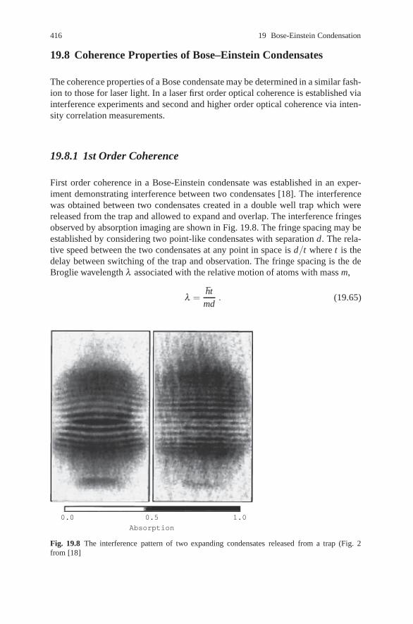
416 19 Bose-Einstein Condensation
19.8 Coherence Properties of Bose–Einstein Condensates
The coherence properties of a Bose condensate may be determined in a similar fash-ion to those for laser light. In a laser first order optical coherence is established viainterference experiments and second and higher order optical coherence via inten-sity correlation measurements.
19.8.1 1st Order Coherence
First order coherence in a Bose-Einstein condensate was established in an exper-iment demonstrating interference between two condensates [18]. The interferencewas obtained between two condensates created in a double well trap which werereleased from the trap and allowed to expand and overlap. The interference fringesobserved by absorption imaging are shown in Fig. 19.8. The fringe spacing may beestablished by considering two point-like condensates with separation d. The rela-tive speed between the two condensates at any point in space is d/t where t is thedelay between switching of the trap and observation. The fringe spacing is the deBroglie wavelength λ associated with the relative motion of atoms with mass m,
λ =htmd
. (19.65)
Absorption
0.0 0.5 1.0
Fig. 19.8 The interference pattern of two expanding condensates released from a trap (Fig. 2from [18]

19.8 Coherence Properties of Bose–Einstein Condensates 417
Their observation confirmed that the fringe spacing became smaller for larger valuesof d.
The observed contrast of the atomic interference was between 50 and 100% .Since the condensates are much larger than the observed fringe spacing they musthave a high degree of spatial coherence. These measurements established the longrange order of the condensate. The theoretical calculations of Sect. 19.6 predictedthat two independent condensates will exhibit interference fringes with a phase thatvaries from run to run. This was not possible to verify in the experiment since me-chanical instabilities were sufficient to generate a random phase.
Spatial interference fringes have also been observed between condensate atomsoutcoupled from a trap demonstrating that the coherence is preserved by the outputcoupler. This may be considered as the first prototype of an “atom laser”.
19.8.2 Higher Order Coherence
Evidence for higher–order coherence, strengthening the analogy between conden-sates and optical laser photons, has also been provided through careful interpretationof some fundamental condensate properties, in particular, of the loss rate of atomsfrom the condensate via three–body recombination and of the mean field energy ofthe condensate.
The atom loss rate due to three–body recombination is directly related to theprobability of finding three atoms close to each other [26], and can therefore act asa probe of the third–order correlation function
g(3)(r,r,r) =〈Ψ†(r)Ψ †(r)Ψ†(r)Ψ (r)Ψ(r)Ψ (r)〉
n(r)3 , (19.66)
where n(r) = 〈Ψ †(r)Ψ (r)〉 is the atomic density. Importantly, the value of this func-tion differs between condensates and thermal clouds by a factor of 3! = 6; in partic-ular, the value of g(3)(r,r,r) for a thermal cloud is a factor of six larger than that fora condensate, implying an atom loss rate due to three–body recombination six timeslarger. The ratio of the noncondensate to the condensate rate constants for this lossprocess was found by Burt et al. [27] to be 7.4±2.0, confirming the presence of atleast third–order coherence in their condensates.
Similarly, Ketterle and Miesner [28] have pointed out that the mean–field energyof a condensate, 〈U〉, provides a direct measure of the second–order correlationfunction,
g(2)(r,r) =〈Ψ †(r)Ψ†(r)Ψ (r)Ψ(r)〉
n(r)2 , (19.67)
through the relationship (see 19.5)
〈U〉=(
2π h2am
)g(2)(0)
∫d3r [n(r)]2 , (19.68)

418 19 Bose-Einstein Condensation
where g(2)(0) ≡ g(2)(r,r), assuming that g(2)(r,r′) depends only on r− r′. Re–analysing condensate data from earlier experiments, they obtain values of g(2)(0)close to 1, as expected for a condensate and differing from that of a thermal cloud,for which g(2)(0) = 2. The reduced value of g(2)(0) for a condensate reflects reduceddensity fluctuations, in direct analogy with the reduced intensity fluctuations of a(photon) laser in comparison with a thermal light source.
We note that g(2)(0) = 1,g(3)(0) = 1, while consistent with a coherent state doesnot distinguish from a number state for g(2)(0) = 1− 1/n,g(3)(0) = 1− 3/n forn∼ 106.
A direct experimental determination of the atom counting statistics may be madeby out coupling atoms from the condensate and letting them fall under the actionof gravity: that is an atom laser. The atoms fall through an optical cavity and mod-ulate the transmission of a coherent laser beam through the cavity by changing the
00.0
0.1
0.2
0.3
0.0
0.5
1.0
1.5
2.0
1 2 3 4 5 6 7 8 9 10
2 4 6 108 12
(a)
(b)
140
Number of events N
Time τ (ms)
gPH(τ
)P
roba
bilit
y P
(N)
Fig. 19.9 The atom number counting statistics for an out-coupled BEC. In (a) the second ordercorrelation functions is shown. (b) the full counting statistics for the atomic number counted in atime T − 1.5 ms. The symbol + indicates the probability for a Poisson distribution with the samemean number n = 1.99 is shown (Fig. 3 from [22])

References 419
absorption and refractive index of the cavity. In the experiment of Ottl et al. [22],using an out-coupled 87Rb BEC, single atoms transiting the driven cavity resultedin a drop in transmission. In this way a Hanbury-Brown Twiss experiment can bedone to determine not only g(2) for the atoms but the full counting statistics. Theresults are shown in Fig. 19.9. We can clearly see the expected value of 1 indicatinga coherent beam.
Exercises
19.1. Show that the condensate Hamiltonian is invariant under the gauge transfor-mation ψ(r)→ ψ(r)eiφ(r).
19.2. The spin coherent states are defined by (see Exercise 15.3)
|α〉= (1 + |α|2)− jj
∑m=− j
(Nm
)1/2
α(m+ j)| j,m〉 (19.69)
where | j,m〉 is the simultaneous eigenstate of J2 and Jz and α is a complexnumber. These states have the same form as the general total number eigen-state for a two-mode condensate given in (19.14) and with the operator cor-respondence given in Sect. 19.7.2. Compute the moments 〈Jk〉 k = x,y,zin terms of α , and show that α lies in the complex plane of the stereo-graphic projection of the Bloch sphere. Also compute the second order mo-ment 〈JzJx〉/N2 and show that for N >> 1 it may be factorised.
19.3. Show that the occupation number representation of the position operator x inthe two-mode approximation is given by
x =2q0
NJx (19.70)
References
1. S.N. Bose: Z. Phys. 26, 178 (1924)2. A. Einstein: Sitzber. Kgl. Preuss. Akad. Wiss. 3 (1925)3. M.H. Anderson, J.R. Ensher, M.R. Matthews, C.E. Wieman, E.A. Cornell: 1995, Science 269,
198 (1995)4. K.B. Davis, M.-O. Mewes, M.R. Andrews, N.J. van Druten, D.S. Durfee, D.M. Kurn,
W. Ketterle: Phys. Rev. Lett. 75, 3969 (1995)5. C.C. Bradley, C.A. Sackett, J.J. Tollett, R.G. Hulet: Phys. Rev. Lett. 75, 1687 (1995)6. Fried, D.G., T.C. Killian, L. Willmann, D. Landhuis, S.C. Moss, D. Kleppner, T.J. Greytak:
Phys. Rev. Lett. 81, 3811 (1998)7. A. Robert, O. Sirjean, A. Browaeys, J. Poupard, S. Nowak, D. Boiron, C.I. Westbrook,
A. Aspect: Science, 292, 461 (2001)

420 19 Bose-Einstein Condensation
8. R. Wynar, R.S. Freeland, D.J. Han, C. Ryu, D.J. Heinzen: Science 287, 1016 (2000)9. M.W. Zwierlein, C.A. Stan, C.H. Schunck, S.M.F. Raupach, A.J. Kerman, W. Ketterle: Phys.
Rev. Lett. 92, 120403 (2004)10. C. Chin, Andrew J. Kerman, V. Vuleti, S. Chu: Phys. Rev. Lett. 90, 033201 (2003)11. C.A. Regal, M. Greiner, D.S. Jin: Phys. Rev. Lett. 92, 040403 (2004)12. O. Mandel, M. Greiner, A. Widera, T. Rom, T.W. Hnsch, I. Bloch: Nature, 425, 937–940
(2003)13. E.M. Lifshitz, L.P. Pitaevskii: Statistical Physics, Part II (Pergamon, Oxford 1980)14. J.A. Dunningham, M.J. Collett, D.F. Walls: Phys. Lett. A, 245, 49 (1998)15. J.C. Eilbeck, P.S. Lomdahl, A.C. Scott: Physica D, 16, 318 (1985)16. R. Gati, M. Albiez, J. Folling, B. Hemmerling, M.K. Oberthaler: Appl. Phys. B 82, 207 (2006)17. D. Ananikian, T. Bergeman: Phys. Rev.A, 73, 013604 (2006)18. M.R. Andrews, C.G. Townsend, H.-J. Miesner, D.S. Durfee, D.M. Kurn, W. Ketterle: Science
275, 637 (1997)19. M.J. Steel, M.J. Collett: Phys. Rev. A 57, 2920 (1998)20. M. Lewenstein, L. You: Phys. Rev. Lett. 77, 3489 (1996b)21. E.M. Wright, D.F. Walls, J.C. Garrison: Phys. Rev. Lett. 77, 2158 (1996)22. A. Ottl, S. Ritter, M.l Kohl, and T. Esslinger, Phys. Rev. Letts., 95, 090404 (2005)23. J. Javanainen, S.M. Yoo: Phys. Rev. Lett. 76, 161 (1996)24. T. Wong, M.J. Collett, D.F. Walls: Phys. Rev. A 54, R3718 (1996)25. G.J. Milburn, J. Corney, E.M. Wright, D.F. Walls, Phys. Rev A. 55, 4318 (1997)26. Yu. Kagan, B.V. Svistunov, G.V. Shlyapnikov: JETP Lett. 42, 209 (1985)27. E.A. Burt, R.W. Ghrist, C.J. Myatt, M.J. Holland, E.A. Cornell, C.E. Wieman: Phys. Rev. Lett.
79, 337 (1997)28. W. Ketterle, H.-J. Miesner: Phys. Rev. A 56, 3291 (1997)
Further Reading
J.R. Anglin, W. Ketterle: Bose-Einstein Condensation of Atomic Gases, Nature, 416, 211 (2002)A. Leggett: Bose-Einstein Condensation in the Alkali Gases, Rev. Mod. Phys. 73, 307 (2001)F. Dalfovo, S. Giorgini, L.P.Pitaevskii, S. Stringari: Theory of Bose-Einstein Condensation in
Trapped Gases, Rev. Mod. Phys. 71, 463 (2001)I. Bloch: Ultracold Quantum Gases in Optical Lattices, Nat. Phys. 1, 23 (2005)A.S. Parkins, D.F. Walls: Bose-Einstein condensation in Dilute Atomic Vapors, Phys Rep. 303, 1
(1998)

Index
Adiabatic elimination, 179, 224Antibunching, photon, 2
laser, 3resonance fluorescence, 205second-order correlation function, 41sub-Poissonian statistics, 42
Atomic decay rate, transverse, 217Atomic operators, collective, 222Atomic optics, 5
Back action evasion, 270Bargmann state, 100Beam splitter, 273Bell inequality, 4, 249
CHSH form, 251parametric down conversion, 254
Bistability, dispersive (linear), 143squeezing spectrum, 147
Bistability, dispersive (nonlinear), 190Fokker–Planck equation, 190
Bistability, optical, 224atomic model, 232noise correlation, 224
Brownian motion, 112Bunching, photon, 2
second-order correlation function, 39, 40sub-Poissonian statistics, 42
Cauchy–Schwarz inequality, 32, 79Cavity, boundary condition, 121Cavity, laser, 229Cavity, two-sided, 127Chaotic field, see Thermal fieldCharacteristic function, 62
optical bistability, 224P representation, 62Q representation, 65
quantum coherence, 283Wigner representation, 63, 107
CHSH inequality, 251Clauser–Horne inequality, 255, 259Coherence, first order optical, 34
Young’s interference experiment, 32Coherence function, 284Coherence, optical, 29Coherence, quantum, 283
visibility, 283Coherent field, 37Coherent state, 12, 109
completeness, 14displacement operator, 12number state expansion, 12Poissonian statistics, 13, 58second-order correlation function, 40, 58
Coherent state two photon, 18Coincidence probability, 261Collisional broadening limit, 204Complementarity, 247Contractive state, 268Correlated state, 247Correlated state, polarization, 248Correlation function, 29
general inequalities, 29phase information, 44
Correlation function, first order, 30Correlation function, higher order, 30Correlation function, phase dependent, 44Correlation function, photon number, 202Correlation function, QND, 267Correlation function, second-order, 39
antibunching, 41bunching, 40coherent state, 41number state, 41
421

422 Index
resonance fluorescence, 205thermal field, 49
Correlation function, two-time, 53Brownian motion, 112input–output formalism, 127master equation, 93Ornstein–Uhlenbeck process, 116parametric oscillator, 136phase diffusion, 237photon counting, 49regularly pumped laser, 238resonance fluorescence, 205two-level atom, 208
Correlation, intensity, 39Hanbury–Brown Twiss experiment, 1,
30, 38parametric amplifier, 73
Covariance matrix, 61Covariance matrix, stationary, 116
Density operator, reduced, 93Detailed balance, 100
harmonic oscillator, 100laser, 232
Duality, wave-particle, 327
Efficiency, quantum, 52Einstein–Podolsky–Rosen paradox, see
Entangled state, EPR paradoxElectric dipole approximation, 203, 225Electromagnetic field, 7
commutation relations, 10Hamiltonian, 10quantisation, 7vacuum state, 10
Entangled state, 261, 310EPR paradox, 80, 247parametric amplifier, 74
Error ellipse, 18coherent state, 18Wigner function, 63
Fock state, see Number stateFokker–Planck equation, 93
degenerate parametric oscillator, 177dispersive bistability, 177, 190Green’s function, 103potential condition, 101stochastic differential equation, 111
Four wave mixing, 3, 279degenerate operation, 277noise correlation, 224phase matching, 254QND, 276
side–band modes, 351squeezing spectrum, 157
Gain, QND, 271, 276–277Gravitational radiation, 267–268
Hanbury–Brown Twiss experiment, 2, 30, 38Harmonic oscillator, damped, 102Harmonic oscillator, master equation, 93
Fokker–Planck equation, 102, 104transition probabilities, 109–110
Harmonic oscillator, 7electromagnetic field, 7
Heat bath, see ReservoirHidden variable theory, 250Homodyne detection, 44–46
four wave mixing, 279–280parametric oscillator, 136–138
Input–output formulation, 127boundary condition, 131laser fluctuations, 138parametric oscillator, 136–138photon counting distribution, 47squeezing spectrum, 140two-time correlation function, 139
Intensity fluctuations, laser, 234–237Interaction picture, 205Interferometer, gravity wave, 159
semiclassical behaviour, 162signal variance, 165total noise, 167
Interferometer, Mach–Zehnder, 309Interferometer, polarization, 173Interferometry, matter, 1, 172, 316Interferometry, optical, 1
squeezed light, 3
Jaynes–Cummings model, 202
Kapitza–Dirac regime, 379Kerr effect, 88, 190KTP crystal, 277
Langevin equation, 112Brownian motion, 112constant diffusion process, 116damped harmonic oscillator, 113four wave mixing, 279input–output formalism, 127
Laser, 2, 231diode, 231gain, 234phase diffusion, 237

Index 423
Scully–Lamb form, 233sub–Poissonian statistics, 3threshold, 234
Laser cooling, 5, 365Laser, fluctuations, 236
intensity, 234–236photon number, 234–235, 240–241pump, 238–241sub-shot noise, 238
Laser, quantum theory, 231Laser, regularly pumped, 239Laser, semiconductor, 238, 242Lens, atomic, 342Linewidth, laser, 237–238Liouvillian operator, 118
Markov approximation, first, 96, 117Master equation, 93
gravitational wave interferometer, 158, 171optical bistability, 178, 224parametric oscillator, 136resonance fluorescence, 205Scully–Lamb laser, 233two-level atom, 205two-time correlation function, 122
Maxwell’s equations, 8Measurement limit, strong, 301Measurement theory, quantum, 283Micro-cavity, 213Microscope, Feynman light, 307Minimum uncertainty state, 15
parametric oscillator, 149squeezed state, 15
Mixture, classical, 290
Noise spectrum, 117Normal ordering, 39, 50
P representation, 118Number state, 10, 57
Observable, QND, 268Optical Bloch equations, 368–371Optical tap, 279, 301Ornstein–Uhlenbeck process, 112
Brownian motion, 112constant diffusion process, 116damped harmonic oscillator, 113
Oscillation threshold, 187
Parametric amplifier, degenerate, 73Parametric amplifier, nondegenerate, 77
selected state, 85thermal reduced state, 85two-mode squeezing, 80
Parametric amplifier, QND, 277Parametric down conversion, 3, 73
Bell inequality, 254Parametric oscillator, 136, 180, 185
squeezed state, 185Parametric oscillator (linear), 3, 131, 136
critical fluctuations, 137Fokker–Planck equation, 136, 138linearisation, 131, 136, 139minimum uncertainty state, 75output correlation matrix, 139squeezing spectrum, 80, 136threshold, 136, 138
Parametric oscillator (nonlinear), 177quadrature variance, 183semiclassical solution, 215threshold distribution, 184
Pauli spin operators, 199Phase decay, collisionally induced, 204Phase diffusion, laser, 237
linewidth, 233two-time correlation function, 237
Phase instability, 152Phase matching, 254Phase operator, Pegg–Barnett, 25Phase operator, Susskind–Glogower, 23Photo-detection, 29, 38, 337Photon counting, 301Photon counting, classical, 46
depletion effects, 50ergodic hypothesis, 48generating function, 47
Photon counting, conditional, 85parametric amplifier, 86
Photon counting distribution, 49Photon counting, nonclassical, 69
number state, 70squeezed state, 70
Photon counting, quantum mechanical, 49Photon number, QND, 279Planck distribution, 58Pointer basis, 296Poissonian pumping, 231Polarization rotator, 254P representation, 58, 61
Bell inequality, 252chaotic state, 59coherent state, 59harmonic oscillator, 99normal ordering, 135quadrature variance, 44
P representation, complex, 68coherent state, 69dispersive bistability, 190, 195
424 Index
harmonic oscillator, 107number state, 65
P representation, generalized, 71, 109bistability, 143harmonic oscillator, 107parametric oscillator, 136, 181
P representation, positive, 71, 115Fokker–Planck equation, 72harmonic oscillator, 107optical bistability, 194parametric oscillator, 177twin beams, 151
Projection postulate, von Neumann, 85Pump depletion, 181
Q function, 65coherent state, 66harmonic oscillator, 106number state, 66squeezed state, 66–67
QND measurement, 4, 268–270pointer basis, 296sub-Poissonian statistics, 238two photon transition, 279
QND measurement, ideal, 268Q parameter, 239Quadrature phase measurement, 44Quadrature phase operator, 81Quantisation, electromagnetic field, 7Quantisation, electron field, 213Quantum nondemolition measurement, see
QND measurementQuantum recurrance phenomena, 90
Kerr effect, 88Quantum regression theorem, 118
resonance fluorescence, 205
Rabi frequency, 390Radiation pressure, 160Raman–Nath regime, 377Recoil energy, 365–366, 372Refractive index, nonlinear, 88Relative states, 298, 301Reservoir, 93
collisional process, 398spectrum, 97–98spontaneous emission, 203two-level atom, 98
Reservoir, squeezed, 96, 144correlation function, 96two-level atom, 98
Reservoir, thermal, 96Resonance fluorescence, 2, 205
elastic scattering, 207
in elastic scattering, 207quantum features, 207–208spectrum, 206
Rotating wave approximation, 128, 190, 199,200, 203, 227, 366
R representation, 67Rydberg atom, 217, 291, 382
Schrodinger cat, 283Second harmonic generation, 146
critical behaviour, 146–147, 152Second harmonic generation, 156–157
twin beams, 155Self pulsing, 147Shot-noise limit, 173
laser, 237, 241Signal-to-noise ratio, 172–173, 302Spectroscopy, photon correlation, 40Spontaneous emission, 203–204
master equation, 205–206Wigner theory, 207
Squeezed state, 15–18, 42–43photon number distribution, 21
Squeezed state, multimode, 22–23Squeezed state, two-mode, 23
parametric amplifier, 74Squeezing, 3, 81–82
four-wave mixing, 279input-output formalism, 127nonlinear susceptibility, 136parametric oscillator, 148
Squeezing, generator, 74parametric amplifier, 74, 77
Squeezing spectrum, 147–148dispersive bistability, 143parametric oscillator, 148–149resonance fluorescence, 205–209
Stability analysis, 145–146Standard quantum limit, 168–171, 267
gravity wave, 267–268State preparation, 270, 271, 276, 333, 335, 384Statistics, photon, 43
laser, 238micromaser cavity, 382regularly pumped laser, 238–241
Statistics, photon counting, 46–47Statistics, Poissonian, 2, 42
coherent state, 13, 58Kerr effect, 88laser, 238
Statistics, sub-Poissonian, 2antibunching, 42bunching, 41laser, 2, 49, 238
Index 425
QND, 268resonance fluorescence, 205
Statistics, super-Poissonian, 42Steady-state solution, 145Stern–Gerlach effect, optical, 381–387Stochastic differential equation, 112–115
Fokker–Planck equation, 112–113gravity wave interferometer, 171Ito equation, 112Langevin equation, 112optical bistability, 190parametric oscillator, 181
Super-Poissonian statistics, 42–44Superposition, coherent, 401Superposition, macroscopic, 4, 401Superposition principle, 283, 325Superposition state, 177, 185, 283, 288, 305,
325, 326, 401Susceptibility, nonlinear, 190Switching time, 188, 191
Thermal field, 49laser, 49second-order correlation function, 52
Transition probability, 29Tunnelling time, 177, 186–190Twin beams, 3, 4, 155
critical behaviour, 156pulsed, 155semiclassical steady-state, 208squeezing spectrum, 156, 157
Two-level atom, 201master equation, 203–204
Uncertainity principle, 7, 12, 16, 83, 267, 270,301, 303, 312
gravity waves, 267
Vector potential, 7, 8, 9, 197Visibility, 32, 34, 289–291
Bell inequality, 251, 256one-photon interference, 259–260quantum coherence, 283
Wavelength, de Broglie, 397Wigner function, 62–65
coherent state, 64covariance matrix, 65harmonic oscillator, 107–109number state, 65parametric amplifier, 83–84squeezed state, 64
Wigner theory, 192resonance fluorescence, 205, 341
Young’s interference experiment, 1, 32coherent superposition, 281, 297correlation function, 32–34, 38experiments, 32, 35, 37, 38quantum explanation of, 1, 37visibility, 32, 34with atoms, 261