Embed Size (px)
Citation preview

Quantum Phase Transitions in Nuclear Collective Models
(Links to Other Concepts)
Pavel CejnarInstitute of Particle & Nuclear Physics, Charles University, Prague
NIL DESPERANDUM !(every suffering has end (when new suffering starts (but through suffering we grow)))

“Now, Nina, do you think you could throw something into the sea?”“I think I could,” replied the child, “but I am sure that Pablo would throw it a great deal further than I can.”“Never mind, you shall try first.”Putting a fragment of ice into Nina’s hand, he addressed himself to Pablo: “Look out, Pablo; you shall see what a nice little fairy Nina is! Throw, Nina, throw, as hard as you can.”
Jules Verne: Off on a CometHector Sarvedac (1877)
Nina balanced the piece of ice two or three times in her hand, and threw it forward with all her strength.A sudden thrill seemed to vibrate across the motionless waters to the distant horizon, and the Gallian Sea had become a solid sheet of ice!

Quantum phase transitions (QPTs)phase transitions at zero temperature driven by interaction strengths
Lattice systems:Studied since 1920’s in connection with magnetism. Usually 2D spin grids that
exhibit a continuous order-disorder transition. Ising, Potts and many other models. Recent overviews: S Sachdev (1999), M Vojta (2003).
Many-body systems: mostly atomic nuclei • DJ Thouless (1961): “collapse of RPA”• R Gilmore (late 1970’s): “ground state (energy) phase transition”
Lipkin model (toy many-body model formulated in terms of quasispin operators) Dicke model (laser phase transition in an interacting atom-field system)
• AEL Dieperink, O Scholten, F Iachello (1980): Interacting boson model (nuclear shape transitions)
• WM Zhang, DH Feng, JN Ginocchio (1987): Fermion dynamical symmetry model(fermionic counterpart of IBM)
• DJ Rowe et al (1998), A Volya, V Zelevinsky (2003)....: various shell-like models describing the ground-state pairing transition

1) Phenomenology (properties of the mean field)Landau theory (1930’s): analysis of the free energy in terms of order parametersCatastrophe theory (1960’s): classification of structurally unstable potentials
2) Mathematical physics (mechanism responsible for QPTs)Pechukas-Yukawa approach: Coulomb-gas analogy for level dynamicsBranch points: level crossings in complex-extended parameter spaceMonodromy (integrable systems): singular class of orbits that disallows analytic description
3) Statistical physics (relation to thermodynamics)Excited-state (finite-temperature) phase transitionsThermodynamic phase transitions
Links to:

Part 1/4:
Nuclear “shape phases”- phenomenology

RF Casten et al (1993)
V Zamfir et al (2002)

Geometric model
Potential energy:
neglect higher-order terms neglect …
depends on 2 internal shape variables
A
Boblate
prolate
spherical432
2222322
3cos)()3()(
bgbb CBAyxCxyxByxAV
++=
++-++=
x
y
…corresponding tensor of momenta
βγ
gba
gba
sin|Re2
cos|Re
PAS2
PAS0
==
==
±y
x
=> nuclear shapes appear as “phases”
quadrupole tensor of collective coordinates (2 shape param’s, 3 Euler angles )
[ ] ( ) .....][5][2
35][5.....][2
5 2)0()0()2()0()0( + ́+´ ́- ́++ ́= aaaaaaapp CBAK
H

Interacting boson model
åå +++ +=lkji
lkjiijklji
jiij bbbbvbbuH,,,,
2,...,2{
+-=+
++ =
mmds
bis-bosons (l=0)
d-bosons (l=2)
• “nucleon pairs with l = 0, 2”• “quanta of collective excitations”
Dynamical algebra: U(6) jiij bbG +=
Subalgebras: U(5), O(6), O(5), O(3), SU(3), [O(6), SU(3)]
]SU(3)[]O(3)[]O(5)[]O(6)[]U(5)[]U(5)[ 2625242322110 CkCkCkCkCkCkkH ++++++=
…generators: …conserves: å +=i
ii bbN
F Iachello, A Arima (1975)
ÉÉÉÉÉÉÉÉ
SU(3)O(5)O(6)
O(3)O(5)U(5)U(6)Dynamical symmetries (extension of standard, invariant symmetries):
063 == kk
0621 === kkk
04321 ==== kkkk
U(5)
O(6)SU(3)
[O(6), SU(3)]

D Warner, Nature 420, 614 (2002).
SU(3)
U(5)
SU(3) O(6)
O(6)
triangle(s)
The simplest, one-component version of the model, IBM-1

21
0
00
||÷÷ø
öççè
æ -µ
lllb
1st order
2nd order
Phase diagram for axially symmetric quadrupole deformation
4
1
32 3cos bgbb ++=±321BAE
order parameter:β=0 spherical, β>0 prolate, β<oblate.
I II III
Triple point
ground-state = minimum of the potential
critical exponent
1st order
Landau (1930’s)

Catastrophe theory
Robert Gilmore: Catastrophe Theory for Scientists and Engineers (1981).“ground-state energy phase transitions”classical & quantal models
Further development:EC Zeeman, V Arnol’d, I Stewart...
The notion of structural stability:“Perturb the Hamiltonian and the topology does not change.”
Theory showing how “continuous causes” can lead to “discontinuous effects”
René Thom (1960’s)

Example:(from EC Zeeman’s lecture, 1995)
many other examples:physics, biology, medicine,economy, sociology, psychology...
bxaxxV ++= 24
Cusp catastrophe
Germ = x4
Codim (no.of free param’s) = 2KbLa µµ ,
1
2
3
4
3
3
4
Germ codim Universal unfolding
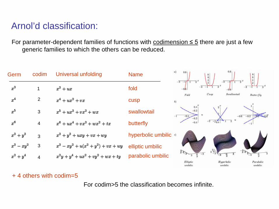
Arnol’d classification:
Name
fold
cusp
swallowtail
hyperbolic umbilic
butterfly
elliptic umbilic
parabolic umbilic
For parameter-dependent families of functions with codimension ≤ 5 there are just a few generic families to which the others can be reduced.
+ 4 others with codim=5For codim>5 the classification becomes infinite.

Cusp catastrophe:
432 bbb +-» BAVBy chosing (i) shift of V and (ii) shift of x (both depending on a,b) we can convert V to the standard cusp form. However,.....
In the shape-phase case we have:

-0.4 -0.2 0.2 0.4
-0.5
0.5
1
...the relevant sign of β is positive, so its negative branches must be disregarded:
spinodal
antispinodal
critical
−a
b
mapping of the shape evolution with),(,1 +¥-¥Î= AB onto the cusp parameter space
deformed
spherical

Part 2/4:
Branch points
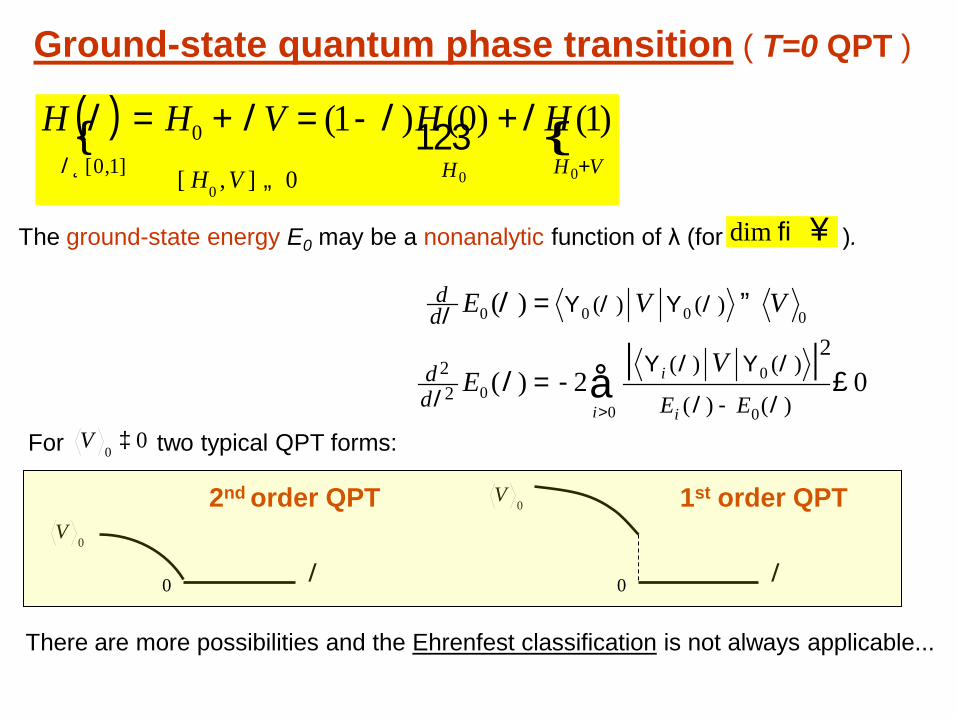
Ground-state quantum phase transition ( T=0 QPT )
( ){ {0],[ 0
00
)1()0()1(0]1,0[ ¹ +Î
+-=+=
VH VHH
HHVHH lllll
321
02)(
)(
0 0
00
0000
)()(
2)()(
)()(
||2
2£-=
º=
å> -
YY
YY
i i
i
EEdd
dd
VE
VVE
ll
lll
lll
l
l
For two typical QPT forms:
The ground-state energy E0 may be a nonanalytic function of λ (for ).
0V
0V
l l
2nd order QPT 1st order QPT
0 0
¥®dim
There are more possibilities and the Ehrenfest classification is not always applicable...
00
³V
úûù
êëé ×
--= )()(1),( d cchhwch QQ
NnH h
ddn ~d ×= +
)2(]~[~)( dddssdQ ´++= +++ cc
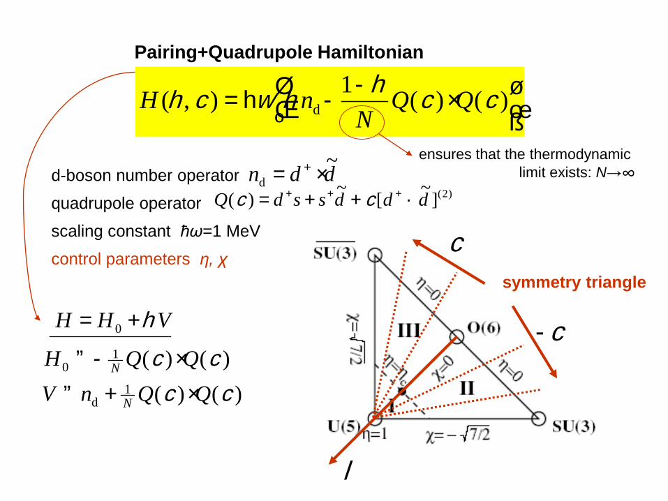
Pairing+Quadrupole Hamiltonian
d-boson number operator
quadrupole operator
scaling constant ħω=1 MeV
control parameters η, χsymmetry triangle
)()()()(
1d
10
0
cccc
h
QQnVQQH
VHH
N
N
×+º
×-º
+=
ensures that the thermodynamiclimit exists: N→∞
c
c-
l

No-crossing rule: In generic situations, eigenvalues of H(λ) with the samesymmetry quantum numbers do not cross:
Instead, one can observe avoided crossings of levels.Rapid structural changes of eigenstates take place atthese sites:
Finite-size precursors of the QPTs are connected with avoided crossings of levels involving the ground-state. These crossings become infinitely closeas the size of the system asymptotically increases...
l[ ]å
¹ --»+
)(2
2
22
)()(
)()()(1)()(
ij ji
jiii EE
V
ll
lylydldllyly
)()( 1 ll +¹ ii EE
)(ly i
)(liE
eigenfunctions
eigenvaluesHamiltonian VHH ll += 0)(
Hill, Wheeler (1953)
QPT mechanism?

QPT mechanism? Multiple avoided crossing of levels
structure I
structure IIg.s.
lcl
Example

Branch pointsTrue degeneracies in the complex plane of λ.They are determined by the conditions
that after elimination yield:
discriminant
2)1( -nn
This has complex conjugate pairs of solutions, where n is dimension of the Hilbert space. For large n numerical calculations become prohibitively difficult.
partial discriminant

The simplest case(dim=2)

0=c
27-=c
20=N
2nd order QPT
1st order QPT
IBM Hamiltonian
withBranch points for J=0
SU(3)-U(5)
O(6)-U(5)
P Cejnar, S Heinze, J Dobeš, AIP Conf. Proc. (2005)
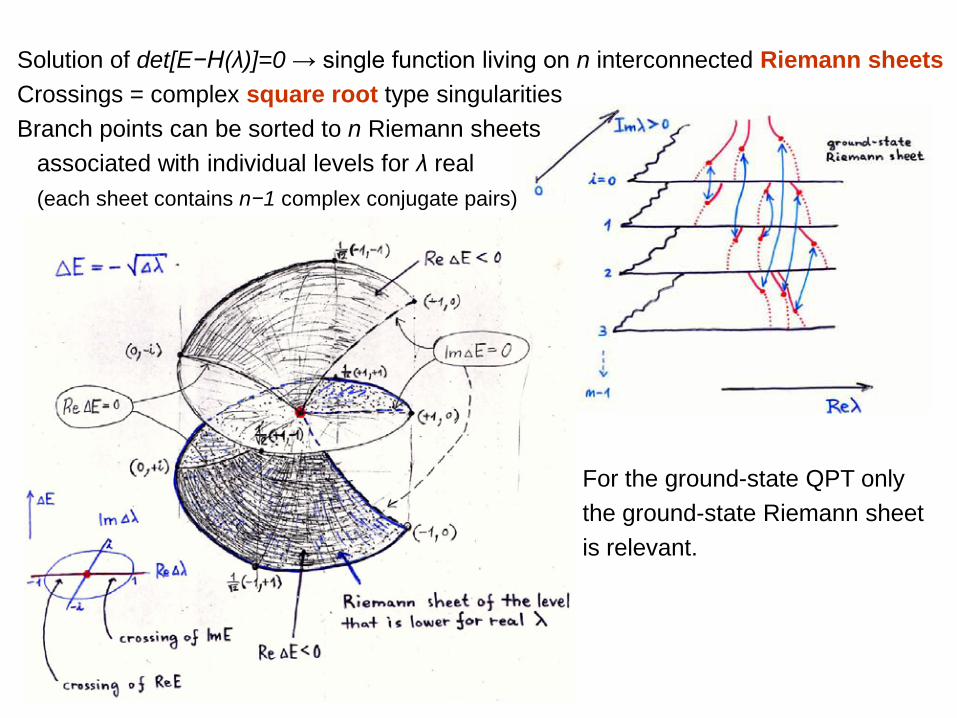
Solution of det[E−H(λ)]=0 → single function living on n interconnected Riemann sheetsCrossings = complex square root type singularitiesBranch points can be sorted to n Riemann sheets
associated with individual levels for λ real (each sheet contains n−1 complex conjugate pairs)
For the ground-state QPT onlythe ground-state Riemann sheetis relevant.

Excursion to thermodynamic phase transitions (TPTs):Zeros of partition function in the complex-temperature plane
CN Yang, TD Lee (1952)S Grossmann, W. Rosenhauer, V Lehmann (1967,69) .....P Borrmann et al (2000) ......
Specific heat = an indirect measure of the density of complex zeros close to real T

Let us assume that there exists an λ↔T analogy between the branch points on the g.s. Riemann sheet and complex zeros of Z, namely, let us consider
1) the ground-state partial discriminant D0 being an analog of Ωth power of thepartition function (where ):
2) the 2D “Coulomb-gas energy” being proportional to free energy:
3) the following expression being an analog of specific heat:
1-µW n
P Cejnar, S Heinze, J Dobeš, PRC 71, 011304(R), (2005).

SU(3)-U(5) 27-=c
O(6)-U(5) 0=c1st order QPT
2nd order QPT
N=10,20,40,80, ...
growth of the maximal value for 1-µW n
1=W
1=W
P Cejnar, S Heinze, J Dobeš, PRC 71, 011304(R), (2005).
1) Branch points accumulateclose to real-λ axis at QPTs
2) The rate of accumulationis quantitatively the same as the accum.of Z=0 pointsclose to real-T axis at TPTs !!!

Part 3/4:
Finite temperatures

Thermodynamic phase transitions (temperature-driven)
Helmholtz free energy 43421321rr
rrrr
ˆˆ
)ˆlnˆ(rt)ˆˆ(rt)(ˆ
SE
THTF --=
)(ln)(0 TZTTF -=
Thermal population of states [ ])ˆexp(tr)()ˆexp()(
1)(ˆ 110 HTTZHT
TZT -- -=-=r
canonical partition function
equilibrium free energy
0)]ˆˆ(tr)ˆˆ(tr[)(
)ˆlnˆ(tr)(
222
022
00
000
322 1
0
³-=
º=
-ºD
-
444 3444 21
TTTEEE
TdTd
dTd
HHTF
TF Srr
rrEntropy is a nondecreasing function of T
In the thermodynamic limit ( ), the entropy (thus F0) may be nonanalytic
2nd order TPT 1st order TPT0S 0S
TT
VNN
/|¥®
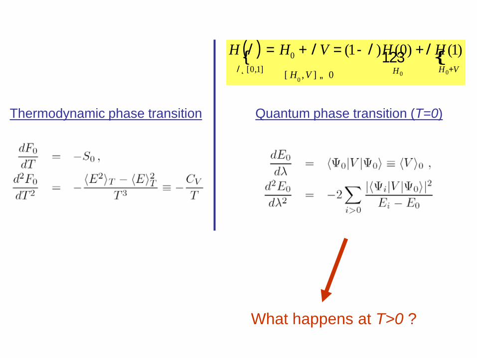
Thermodynamic phase transition Quantum phase transition (T=0)
What happens at T>0 ?
( ){ {0],[ 0
00
)1()0()1(0]1,0[ ¹ +Î
+-=+=
VH VHH
HHVHH lllll
321
λ
T F(λ,T)
λ
E
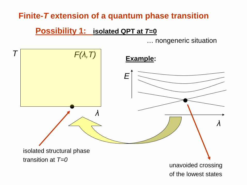
unavoided crossingof the lowest states
isolated structural phase transition at T=0
Possibility 1: isolated QPT at T=0… nongeneric situation
Example:
Finite-T extension of a quantum phase transition

λ
T F(λ,T)
continuous phase separatrix in the (λ,T) plane
TETF
STF
TT
T2
0
00
322 1),(
),(
D=
=
¶¶
¶¶ -
l
l
Possibility 2: QPT survives inclusion of finite T
[ with possible endpoint (λt,Tt) ]
?),(
?),(
0
0
22
=
=
¶¶¶¶
TF
TF
l
l
l
l
… expected situation
Finite-T extension of a quantum phase transition

Thermodynamic phase transition Quantum phase transition (T=0)
Finite-T extension of a quantum phase transition
“Excited-state quantum phase transition” (T>0)

λ
T F(λ,T)
Nonzero density of Z=0 pointsas ImT→0 (thermodynamic limit)
Nonzero density of branch pointsas Imλ→0 (thermodynamic limit)Surmise: )(
),()( br
)()(
br
1
lrl
lrl
(i)
i
ETT
TZe i
å--
=density on the i th Riemann sheet,or:
T>0 relevant density
?
Finite-T extension of a quantum phase transition
)(lim),(lim )(brIm0Im
)(br0Im
lrlr lll
ii
®®

Part 4/4:
Monodromy andexcited-state QPTs
in integrable systems

N=80all levels with J=0
ground-state phase transition (2nd order)
What about “phase transitions” for excited states (if any) ???
E
η
in the sense of nonanalytic evolutions of and
2nd order
1st order
O(6)-U(5)
)()( lyl iiE

General analytic approach: To employ the basis(condensate of N−k bosons) plus
(k bosons in single-particle states)with k=0...N and evaluate the dependence ofeigenvalues on λ. (Work in progress: F Iachello, M Caprio...)
Approach discussed here: based on some analogies in classical mechanics (monodromy)and on some specific analytic approximations(shifted oscillator approximation). Not systematicand applicable only in integrable systems [i.e., along O(6)−U(5) in the IBM], nevertheless still yielding some new insights...
N=80all levels with J=0
E
ηground-state phase transition (2nd order)
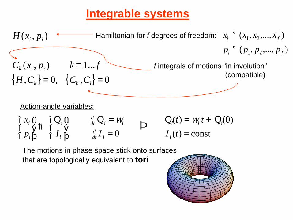
Integrable systems
{ } { } 0,,0,...1),(
),(
===
lkk
iik
ii
CCCHfkpxC
pxH Hamiltonian for f degrees of freedom:
),...,,(
),...,,(
21
21
fi
fi
ppppxxxx
º
º
f integrals of motions “in involution”(compatible)
Action-angle variables:
const)()0()(
0 =Q+=Q
==Q
þýü
îíìQ
®þýü
îíì Þ
tItt
IIpx
i
iii
idtd
iidtd
i
i
i
i ww
The motions in phase space stick onto surfaces that are topologically equivalent to tori

Monodromy in classical and quantum mechanics
Invented: JJ Duistermaat, Commun. Pure Appl. Math. 33, 687 (1980).
Promoted: RH Cushman, L Bates: Global Aspects of Classical Integrable Systems(Birkhäuser, Basel, 1997).
Simplest example: spherical pendulum
x
z
y
Etymology: Μονοδρoμια = “once around”
ρ
( ) zpppH zyx +++= 22221
01222
=++=++
zyx zpypxpzyx
Hamiltonian
constraints
Conserved angular momentum: xyz ypxpL -=
{ } Þ= 0, PoissonzLH 2 compatible integrals of motions, 2 degrees of freedom(integrable system)

-1 -0.5 0.5 1
-2
-1
1
2
r
rp
trajectories with E=1, Lz=0
Singular bundle of orbits: point of unstable equilibrium(trajectory needs infinite time to reach it)
“pinched torus”
…corresponding lattice of quantum states:

It is impossible to introduce a global system of 2 quantum numbersdefining a smooth grid of states:
q.num.#1: z-component of ang.momentum mq.num.#2: ??? candidates: “principal.q.num.” n, “ang.momentum” l, combination n+m
K Efstathiou et al., Phys. Rev. A 69, 032504 (2004).“crystal defect”of the quantum lattice
m m m
low-E high-E

Another example: Mexican hat (champagne bottle) potential
x
y
V
E=0
principal q.num. 2nrad+mradial q.num. nrad
Pinched torus of orbits: E=0, Lz=0
Crystal defect of the quantum lattice
-1 -0.5 0.5 1
-0.6
-0.4
-0.2
0.2
0.4
0.6
rrp
( ) 422221 rr bappH yx +-+=
MS Child, J. Phys. A 31, 657 (1998).

( ))
~~)(()3(
~)0(
~
dd2
21
d
)]5([ ddddnnC
ssddPdssdQ
ddn
O ××-+=
-×=
+=
×=
++
++++
++
+
O(6)-U(5) transition
hhhh
34'34
-»-»a
{ })4(1'1'
)0()0(1)0,(
)]5(O[222d
2d
+--
+÷øö
çèæ -
+=
×-
-==
+ NNCN
PPN
nN
a
QQN
nNN
H
hhh
hhch
)3( +vv “seniority”
42222cl )1(
245)1(
2bhbhpbhph
-+-
+-+=® HNH
kinetic energy Tcl potential energy Vcl
22222
÷÷ø
öççè
æ+=+=
bp
pppp gbyx
222 yx +=b
Classical limit for J=0 :
J=0 projected O(5) “angular momentum”
xyNv yx pppg -=«
22
10
)]5([O2 gp¾¾ ®¾=J
CN
The O(6)-U(5) transitional system is integrable: the O(5) Casimir invariant remains an integral of motion all the way and seniority v is a good quantum number.
]1,0[],2,0[],2,0[ ÎÎÎ gb ppb

422422
cl
11 )~
()~
(2
bbpb +-=
+×+-= ++++
H
dssddssdHNN
2212
21
cl
11
bp +=
=
H
nH dNN
422
452222cl
11
)1()1(
)0()0(2
bhbpbhp hh
hh
-++-+=
×-=-
-
H
QQnHNdNN
O(6) U(5)
0 14/5h
O(6)-U(5) transition
deformed g.s. spherical g.s.

η=0.6
pinched torus
Poincaré surfaces of sections:
22-
Μονοδρoμια
M Macek, P Cejnar, J Jolie, S Heinze, Phys. Rev. C 73, 014307 (2006).

( ) )()(ˆTr )( atoryllioscsmooth
Ω
EEHEE(E)
rrdr +=-=
µ43421
Available phase-space volume at given energyconnected to the smooth component of quantum level density
ò=W)(
)(
max
min
);(2 max
);(2)(E
E
dEhE
Ep
b
b
bbbp
bb
321
)(EW
minb maxb
β
E
0
E0
singular tangent
)(EdEd
W
( )ò -=W ff dqdpqpHEE ),()( d
Volume of the “enveloping” torus:
P Cejnar et al., subm.to J.Phys.A

g
b
b
g
w
w==
TT
RClassification of trajectories by the ratio of periods associated with
g
b
mm
=Roscillations in β and γ directions. For rational the trajectory is periodic:
M Macek, P Cejnar, J Jolie, S Heinze,Phys. Rev. C 73, 014307 (2006).

R
E
E=0
Spectrum of orbits(obtained in a numerical simulation involving ≈ 50000 randomly selectedtrajectories)
η=0.6
R≈2“bouncing-ball orbits”(like in spherical oscillator)
R>3“flower-like orbits”(Mexican-hat potential)
At E=0 the motions change theircharacter from O(6)- to U(5)-liketype of trajectories
M Macek, P Cejnar, J Jolie, S Heinze,Phys. Rev. C 73, 014307 (2006).
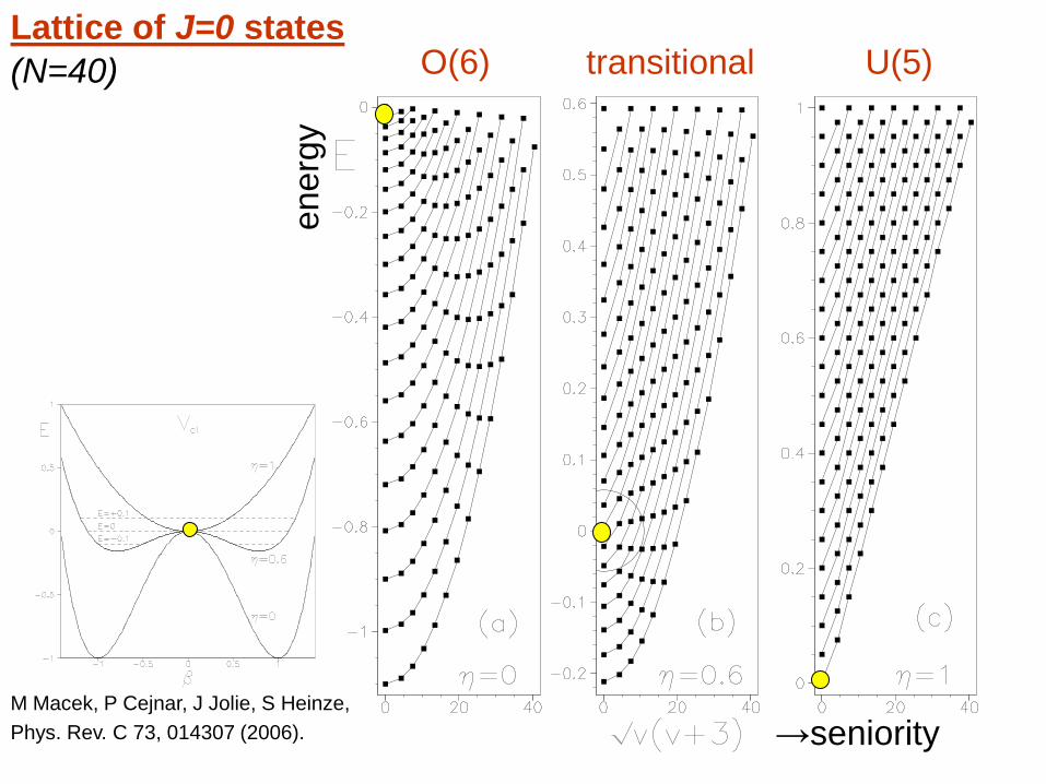
O(6) transitional U(5)
→seniority
ener
gy
Lattice of J=0 states(N=40)
M Macek, P Cejnar, J Jolie, S Heinze, Phys. Rev. C 73, 014307 (2006).

E=0
J=0 level dynamics across the O(6)-U(5) transition (all v’s)
N=40
S Heinze, P Cejnar, J Jolie, M Macek,Phys. Rev. C 73, 014306 (2006).

Wave functions in an oscillator approximation:DJ Rowe, Phys. Rev. Lett. 93, 122502 (2004), Nucl. Phys. A 745, 47 (2004).
)()()()(
)()()()(
2
2
22111
11 22
xxxx
xExxx
EH
idxd
Nidxd
NiNi
iiNiddNiddidd
iii
nHnnHnnHn
yyyy
yyyy
+±=±
=-+++
Y=Y
-+
)(12 xnNnx iid
d yºY-=
H oscillator with x-dependent mass:
N=60, v=0i=1 i=2
O(6) limit
O(6)-U(5)
x may be treated as a continuous variable (N→∞)
Method applicable along O(6)-U(5) transition for N→∞ and states with rel.seniority v/N=0 :
O(6) quasi-dynamical symmetry breaks down once the edge of semiclassical wave function reaches the nd=0 or nd=N limits.
nd
¾¾¾ ®¾¥®N ( ) 0
20osc )( ExxL
dxdxK
dxdH +-+-=

)0()0(1)(2d QQ
Nn
NNH
×-
-=hhh
}
( )44444 844444 76
443442143421
876h
)(
)()(
)(
2
2
2osc11
00
1
2)1(4
452)1(4
14)( ][][xV
Ex
xm
xxd
dxxd
dN
H
h
hh
h hh
hhh
µ
µ
µ
- --
--
-+--=
-
For v=0 eigenstates of we obtain:
h
-0.2
0
0.2 0
0.25
0.5
0.75
1
-1-0.75-0.5
-0.250
-0.2
0
0.2
h
0)( £xVh
x
0.2
0.4
0.6
0.8
-0.2
-0.10.1
0.2 x
h
[ ] [ ]maxmin2 ,1,11 xxxx N
nd º+-ÎÞ-=
0.2 0.4 0.6 0.8
-1
-0.8
-0.6
-0.4
-0.2
ground-state phasetransition
=> approximation holds for energies below 0)()( minup == xVE hh
η=0.8
)(0 hE1-
P Cejnar et al., subm.to J.Phys.A
At E=0 all v=0 states undergo a nonanalytic change.

-0.25 -0.2 -0.15 -0.1 -0.05 0.05
5
10
15
20
25
30
35
x1-
0=E 0<E
x-dependence of velocity–1( classical limit of |ψ(x)|2 )
)(1
minxx -µ 2/1
end )(1xx -
µ
At E=0 all v=0 states undergo a nonanalytic change.
Effect of m(x)→∞ for x → –1
Similar effect appears in the β-dependence of velocity–1 in the Mexican hat at E=0
1/β-divergence 0001 =«=«-= bdnx
ßIn the N→∞ limit the average <nd >i →0 (and <β >i →0) as E→0.
P Cejnar et al., subm.to J.Phys.A

i=1 i=10
i=20 i=30|Ψ(nd )|2
å-=dn
didii nPnPS )(ln)(U(5)
U(5) wave-function entropy
quasi-O(6)quasi-U(5)
v=0↓
Eup=0
S Heinze, P Cejnar, J Jolie, M Macek, PRC 73, 014306 (2006).
N=80

4444444 34444444 21
444 8444 76
)(
)1(2
452
)1()1(2
eff
)(
422
2222
cl
b
bhbhb
hddhpbhhb
b
V
H
V
-+-
++-+úûù
êëé -+=
( ) 2222
10
)]5([O2 gpd ¾¾ ®¾º«=JN
vN
C
constant & centrifugal terms
è!!!!20.1
0.2
0.3
0.4
0.5
0.6
è!!!!2-0.1
0.1
0.2
0.3
è!!!!2-0.1
0.1
0.2
0.3
0.4
0.5
0.6
4Nv = 2
Nv =0=veffV
b
422
22cl
1 )1(2
45)1(20
bhbhbp
pbhh gb -+
-+
úúû
ù
êêë
é÷÷ø
öççè
æ+úû
ùêëé -+=¾¾ ®¾
=HH
JN
Any phase transitions for non-zero seniorities?
0 0.2 0.4 0.6 0.8 1
0.5
0.6
0.7
0.8
0.9
1
d
10 =b
h 10
For δ≠0 fully analytic evolution of the minimum β0 and min.energy Veff(β0)=> no phase transition !!!
effV
P Cejnar et al., subm.to J.Phys.A

N=80
v=0
v=18
2nd ordercontinuousground stateexcited states
0up =E
J=0 level dynamics for separate seniorities
no phase transition
(maybe with noEhrenfest classif.)
P Cejnar et al., subm.to J.Phys.A

Surprising analogy:
M Macek et al, in preparation
O(6)-U(5)
“semi-regular arc”
O(6)SU(3)
U(5)
Does this imply similar QPT behavior in the arc? How to define monodromy in nonintegrable regimes?Phase transitions for other paths in the triangle?
(Alhassid et al, 1991)
J=0N=40
η
Collaborators: Michal Macek, Pavel Stránský (Prague)
Jan Dobeš (Řež)
Stefan Heinze, Jan Jolie (Cologne)
Thanks to: Vladimir Zelevinsky (Michigan)
David Rowe (Toronto)Franco Iachello, Rick Casten, Yoram Alhassid (Yale)
Zdeněk Pluhař (Prague)
.................

APPENDICES

n1=nrad+v/3
n2=nrad+2v/3
radial quantum number nrad
principal quantum number N=2nrad+m
angular-momentum quantum number m0 2 3 41
0
01
1
2
2
3
3
4
4… yes, but only for nd=3k
differences between the O(2) and J=0 projected O(5) angular momenta
*
*m
E
[V(V+3)]½
E
2212
21
cl
11
bp +=
=
H
nH dNN
Quantum lattice of states: U(5) limit
Analogy with standard isotropic 2D harmonic oscillator:_________________________________________________________
N=40

O(5) quantum number: seniority v
O(6) quantum number: σ
O(6) limit
422422
cl
11 )~
()~
(2
bbpb +-=
+×+-= ++++
H
dssddssdHNN
[V(V+3)]½
N=40

Transitional case
O(6)-liketype of cells
U(5)-liketype of cells
Redistribution of levels between O(6) and U(5) multiplets
E=0
422
45
2222cl
11
)1()1(
)0()0(2
bhbpbhp
h
h
hh
-++-+=
×-=
-
-
H
QQnHNdNN
[V(V+3)]½
ΜονοδρoμιαPinched torus of E=v=0orbits connected with the unstable equilibrium at β=0
M Macek, P Cejnar, J Jolie, S Heinze, Phys. Rev. C 73, 014307 (2006).
N=40

≈2x
v=0
v=18
EnergySpacing of neighboring levels
N=80
J=0 level dynamics across the O(6)-U(5) transition (separate v’s)
“shock wave”
S Heinze, P Cejnar, J Jolie, M Macek,Phys. Rev. C 73, 014306 (2006).
( )( )
( )[ ]421
1,,3
2
1fluct cos p
mp
mm
mp n
mr --= åå
¥
=
rrh
r
r
hh
rESrgr
TE
r E
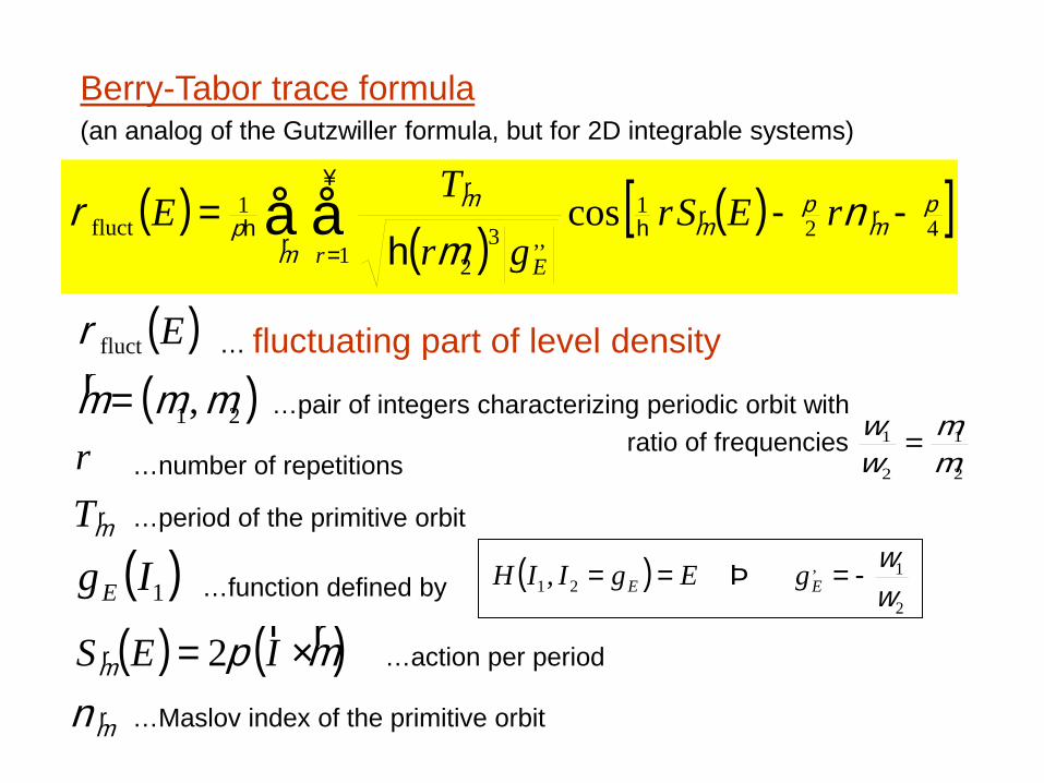
Berry-Tabor trace formula(an analog of the Gutzwiller formula, but for 2D integrable systems)
( )Efluctr
mrT
( ) ( )mpmrr
r ×= IES 2
( )21, mmm =r
2
1
2
1
mm
ww
=
… fluctuating part of level density
…pair of integers characterizing periodic orbit with ratio of frequencies
…period of the primitive orbit
r …number of repetitions
…action per period
( )1IgE ( )2
1,21, w
w-=Þ== EE gEgIIH…function defined by
mn r …Maslov index of the primitive orbit

1st10th
20th30th
average numbers of d-bosons
v=0
v=18
Heinze, Cejnar, Jolie, Macek,PRC (2006).


IBM classical limitGeneral method: coherent states (Schrödinger, Glauber, Gilmore, Perelomov,....) Specific realization: RL Hatch, S Levit, Phys. Rev. C 25, 614 (1982)
Y Alhassid, N Whelan, Phys. Rev. C 43, 2637 (1991)____________________________________________________________________________________
● use of Glauber coherent states
aa HH =cl
å +=ºm
maaaa 22s ||||NN
● boson number conservation (only in average)
complex variables contain coordinates & momentaa
● classical limit:
[ ]mmmaa -- +-=® ipq
N)(
21 ( ) 2£+å 22
mmm qp
¥®N
fixed
10 real variables:(2 quadrupole deformation parameters, 3 Euler angles,5 associated momenta)
0)exp( s|| 2
21
å ++- +=m
ma aaa dse
● angular momentum J=0 Euler angles irrelevant only 4D phase space
(12 real variables)
2 coordinates (x,y) or (β,γ)
restricted phase-space domainÞ Þ
● classical Hamiltonian
● result: ( )4
232
22
3cos1
),,,(21
2
bgbb
ppgbp
b
gbbp
bg
CBAV
fK
T
+-+=
+úûù
êëé += Similar to GCM but with position-dependent
kinetic terms and higher-order potential terms
[ ]2,0Îb