Embed Size (px)
Citation preview
Quantum Physics Notes
J D CresserDepartment of PhysicsMacquarie University
September 5, 2001
Contents
1 Introduction 4
2 The Early History of Quantum Mechanics 7
3 The Wave Function 10
3.1 The Harmonic Wave Function . . . . . . . . . . . . . . . . . . . . . . . . . . 10
3.2 Wave Packets . . . . . . . . . . . . . . . . . . . . . . . . . . . . . . . . . . . 11
3.3 The Heisenberg Uncertainty Principle . . . . . . . . . . . . . . . . . . . . . 13
3.3.1 The Size of an Atom . . . . . . . . . . . . . . . . . . . . . . . . . . . 14
3.3.2 The Minimum Energy of a Simple Harmonic Oscillator . . . . . . . 16
4 The Two Slit Experiment 18
4.1 An Experiment with Bullets . . . . . . . . . . . . . . . . . . . . . . . . . . . 18
4.2 An Experiment with Waves . . . . . . . . . . . . . . . . . . . . . . . . . . . 20
4.3 An Experiment with Electrons . . . . . . . . . . . . . . . . . . . . . . . . . 21
4.4 Probability Amplitudes . . . . . . . . . . . . . . . . . . . . . . . . . . . . . 23
4.5 The Fundamental Nature of Quantum Probability . . . . . . . . . . . . . . 25
5 Wave Mechanics 26
5.1 The Probability Interpretation of the Wave Function . . . . . . . . . . . . . 26
5.2 Expectation Values and Uncertainties . . . . . . . . . . . . . . . . . . . . . 27
5.3 Particle in an Infinite Potential Well . . . . . . . . . . . . . . . . . . . . . . 28
5.3.1 Some Properties of Infinite Well Wave Functions . . . . . . . . . . . 31
5.4 The Schrodinger Wave Equation . . . . . . . . . . . . . . . . . . . . . . . . 36
5.5 Is the Wave Function all that is Needed? . . . . . . . . . . . . . . . . . . . . 37
CONTENTS 2
6 Particle Spin and the Stern-Gerlach Experiment 38
6.1 Classical Spin Angular Momentum . . . . . . . . . . . . . . . . . . . . . . . 38
6.2 Quantum Spin Angular Momentum . . . . . . . . . . . . . . . . . . . . . . . 39
6.3 The Stern-Gerlach Experiment . . . . . . . . . . . . . . . . . . . . . . . . . 41
6.4 Quantum Randomness in Spin Measurements . . . . . . . . . . . . . . . . . 43
6.4.1 Incompatible Measurements of Spin Components . . . . . . . . . . . 44
6.4.2 Probabilities for Spin . . . . . . . . . . . . . . . . . . . . . . . . . . . 47
6.5 Quantum Interference for Spin . . . . . . . . . . . . . . . . . . . . . . . . . 49
7 Probability Amplitudes 54
7.1 The State of a System . . . . . . . . . . . . . . . . . . . . . . . . . . . . . . 55
7.2 The Two Slit Experiment Revisited . . . . . . . . . . . . . . . . . . . . . . 56
7.2.1 Sum of Amplitudes in Bra(c)ket Notation . . . . . . . . . . . . . . . 58
7.2.2 Superposition of States for Two Slit Experiment . . . . . . . . . . . 58
7.3 The Stern-Gerlach Experiment Revisited . . . . . . . . . . . . . . . . . . . 60
7.3.1 Superposition of States for Spin Half . . . . . . . . . . . . . . . . . . 63
8 Vector Spaces in Quantum Mechanics 66
8.1 Vectors in Two Dimensional Space . . . . . . . . . . . . . . . . . . . . . . . 66
8.1.1 Linear Combinations of Vectors – Vector Addition . . . . . . . . . . 66
8.1.2 Inner or Scalar Products . . . . . . . . . . . . . . . . . . . . . . . . . 67
8.2 Spin Half Quantum States as Vectors . . . . . . . . . . . . . . . . . . . . . . 68
8.3 The General Case of Many Intermediate States . . . . . . . . . . . . . . . . 75
8.4 General Mathematical Description of a Quantum System . . . . . . . . . . 76
8.4.1 State Space . . . . . . . . . . . . . . . . . . . . . . . . . . . . . . . . 76
8.4.2 Probability Amplitudes and the Inner Product of State Vectors . . . 77
8.5 Constructing a State Space . . . . . . . . . . . . . . . . . . . . . . . . . . . 80
9 Operations on States 83
9.1 Definition and Properties of Operators . . . . . . . . . . . . . . . . . . . . . 83
9.1.1 Definition of an Operator . . . . . . . . . . . . . . . . . . . . . . . . 83
9.1.2 Properties of Operators . . . . . . . . . . . . . . . . . . . . . . . . . 84
9.2 Action of Operators on Bra Vectors . . . . . . . . . . . . . . . . . . . . . . 89
9.3 The Hermitean Adjoint of an Operator . . . . . . . . . . . . . . . . . . . . . 92
9.3.1 Hermitean and Unitary Operators . . . . . . . . . . . . . . . . . . . 93
9.4 Eigenvalues and Eigenvectors . . . . . . . . . . . . . . . . . . . . . . . . . . 94
9.4.1 Eigenstates and Eigenvalues of Hermitean Operators . . . . . . . . . 95
9.4.2 Continuous Eigenvalues . . . . . . . . . . . . . . . . . . . . . . . . . 97
9.5 Dirac Notation for Operators . . . . . . . . . . . . . . . . . . . . . . . . . . 100
CONTENTS 3
10 Representations of State Vectors and Operators 104
10.1 Representation of Vectors as Column and Row Vectors . . . . . . . . . . . . 104
10.1.1 Column Vectors . . . . . . . . . . . . . . . . . . . . . . . . . . . . . 105
10.1.2 Row Vectors . . . . . . . . . . . . . . . . . . . . . . . . . . . . . . . 106
10.1.3 Probability Amplitudes, Inner Products and Bra Vectors . . . . . . 107
10.2 Representations of State Vectors and Operators . . . . . . . . . . . . . . . . 108
10.2.1 Representation of Ket and Bra Vectors . . . . . . . . . . . . . . . . . 108
10.2.2 Representation of Operators . . . . . . . . . . . . . . . . . . . . . . . 110
10.2.3 Properties of Matrix Representations of Operators . . . . . . . . . . 113
10.2.4 Eigenvectors and Eigenvalues . . . . . . . . . . . . . . . . . . . . . . 116
10.2.5 Hermitean Operators . . . . . . . . . . . . . . . . . . . . . . . . . . . 117
11 The Basic Postulates of Quantum Mechanics 120
11.1 Quantum States are Vectors in a Hilbert Space . . . . . . . . . . . . . . . . 120
11.2 Observables of a Quantum System . . . . . . . . . . . . . . . . . . . . . . . 121
11.3 Completeness of Eigenstates of an Observable . . . . . . . . . . . . . . . . . 123
11.4 Probability Interpretation . . . . . . . . . . . . . . . . . . . . . . . . . . . . 123
11.5 Change of State by Measurement . . . . . . . . . . . . . . . . . . . . . . . . 124
Chapter 1
Introduction
The world of our every-day experiences – the world of the not too big (compared to,say, a galaxy), and the not too small, (compared to something the size and mass of anatom), and where nothing moves too fast (compared to the speed of light) – is the worldthat is mostly directly accessible to our senses. This is the world usually more thanadequately described by the theories of classical physics that dominated the nineteenthcentury: Newton’s laws of motion, including his law of gravitation, Maxwell’s equationsfor the electromagnetic field, the three laws of thermodynamics. These classical theoriesare characterized by, amongst other things, the notion that there is a ‘real’ world out there,one that has an existence independent of ourselves, in which, for instance, objects have adefinite position and momentum which we could measure to any degree of accuracy, limitedonly by our experimental ingenuity. According to this view, the universe is evolving in away completely determined by these classical laws, so that if it were possible to measurethe position and momenta of all the constituent particles of the universe, and we knew allthe forces that acted between the particles, then we could in principle predict to what everdegree of accuracy we desire, exactly how the universe (including ourselves) will evolve.Everything is predetermined – there is no such thing as free will, there is no room forchance. Anything apparently random only appears that way because of our ignorance ofall the information that we would need to have to be able to make precise predictions.
This rather gloomy view of the nature of our world did not survive long into the twentiethcentury which saw the formulation of a new set of fundamental principles that provides aframework into which all physical theories must fit, and to that extent all natural phenom-ena are governed to a greater or lesser extent by its laws: quantum mechanics. One of thecrucial features of quantum mechanics is the loss of determinancy: irreducible randomnessis built into the laws of nature. The world is inherently probabilistic in that events canhappen without a cause, a fact first stumbled on by Einstein, but never fully accepted byhim.
Quantum mechanics is often thought of as being the physics of the very small, but thisis true only insofar as the fact that peculiarly quantum effects are most readily observedat the atomic level. But in the everyday world that we usually experience, where theclassical laws of Newton and Maxwell seem to be able to explain so much, it quickly be-comes apparent that classical theory is unable to explain many things e.g. why a solid is‘solid’, or why a hot object has the colour that it does. Beyond that, quantum mechanicsis needed to explain radioactivity, the chemical properties of matter, how semiconductingdevices work, superconductivity, the interaction between light and matter (leading to de-scribing what makes a laser do what it does), the properties of elementary particles such asquarks, muons, neutrinos, . . . . Even on the very large scale, quantum effects leave their
Chapter 1 Introduction 5
mark in unexpected ways: the galaxies spread throughout the universe are believed tobe macroscopic manifestations of microscopic quantum-induced inhomogeneities presentshortly after the birth of the universe, when the universe itself was tinier than an atomicnucleus and almost wholly quantum mechanical. Indeed, the marriage of quantum me-chanics – the physics of the very small – with general relativity – the physics of the verylarge – is believed by some to be the crucial step in formulating a general ‘theory of ev-erything’ – superstring theory – that will hopefully contain all the basic laws of nature inone package. The impact of quantum mechanics on our view of the world and the naturallaws that govern it, cannot be underestimated. But the subject is not entirely esoteric.Its consequences have been exploited in many ways that have an immediate impact on thequality of our lives. It has been estimated that the economical impact of quantum me-chanics cannot be ignored: about 30% of the gross national product of the United Statesis based on inventions made possible by quantum mechanics. If anyone aims to have any-thing like a broad understanding of the sciences that underpin modern technology, as wellas obtaining some insight into the modern view of the character of the physical world,then some knowledge and understanding of quantum mechanics is mandatory.
As we have just seen, quantum mechanics is essential in providing a framework of physicaland mathematical principles with which we attempt to understand the physical nature ofthe world in which we live. Its success in doing just that has been extraordinary. Yet forall of that, and in spite of the fact that the theory is now roughly 100 years old, if Planck’stheory of black body radiation is taken as being the birth of quantum mechanics, it as truenow as it was then that no one truly understands the theory, even though by followingits principles, it is possible to provide an explanation of everything from the state of theuniverse immediately after the big bang, to the structure of DNA, to the colour of yoursocks.
The most familiar version of the quantum theory goes by the name ‘wave mechanics’, andits most familiar application is to describing the structure of matter at the atomic level:atomic, molecular and solid state physics, built as it is around the wave function ψ andthe interpretation of |ψ|2 as giving the probability of finding a particle in some region inspace. But quantum mechanics is much more than the mechanics of the wave function,and its applicability goes way beyond atomic, molecular or solid state theory. Quantummechanics is a set of fundamental principles that presumably apply to all physical systems:to the electromagnetic field and the other force fields of nature, to quarks and electronsand other fundamental particles, which can be created or destroyed and which possess suchproperties as spin, charge, colour, flavour, to many particle systems such as the electronsin a metal, or photons in a laser beam. These principles embody fundamental physical andphilosophical issues that can be abstracted from and studied independently of any physicalsystem that could potentially display them. It is these principles abstracted in this waythat constitute quantum mechanics. To describe the quantum properties of such a widevariety of physical phenomena, and to provide a language that contains all of the basicprinciples of quantum mechanics without being tied to the notion of the wave function, amore general perspective is required.
A deeper look at what constitutes quantum theory shows that wave mechanics is butone mathematical manifestation or representation of an underlying, more general theorywhose principles can be applied to all of the above examples. The language of this moregeneral theory is the language of vector spaces, of state vectors and of Hermitean operatorsand observables, of eigenvalues and eigenvectors, of linear superpositions of states, oftime development operators, and so on. This language contains the essence of quantummechanics, and it is this general version of quantum mechanics that this course is designedto introduce you to. The aim in mind is to show just how all-encompassing the theory is,
Chapter 1 Introduction 6
and just how strange it is.
The starting point will be a quick review of the history of quantum mechanics, with theaim of summarizing the essence of the wave mechanical point of view. Following this, astudy will be made of the one experiment that is supposed to embody all of the mysteryof quantum mechanics – the double slit interference experiment. A closer analysis of thisexperiment also leads to the introduction of a new notation – the Dirac notation – alongwith a new interpretation in terms of vectors in a Hilbert space. Subsequently, workingwith this general way of presenting quantum mechanics, the physical content of the theorywill be developed.
Chapter 2
The Early History of QuantumMechanics
In the early years of the twentieth century, Max Planck, Albert Einstein, Louis de Broglie,Neils Bohr, Werner Heisenberg, Erwin Schrodinger, Max Born, Paul Dirac and otherscreated the theory now known as quantum mechanics. The theory was not developed ina strictly logical way – rather a series of guesses inspired by profound physical insightand a thorough command of new mathematical methods was sewn together to create atheoretical edifice whose predictive power is such that quantum mechanics is consideredthe most successful theoretical physics construct of the human mind. Roughly speakingthe history is as follows:
Planck’s Black Body Theory (1900) In an attempt to understand the form of thespectrum of the electromagnetic radiation emitted by an object in thermal equilibrium atsome temperature (a black body), Planck was forced to propose that the atoms makingup the object absorbed and emitted light of (angular) frequency ω in multiples of a fun-damental unit of energy, or quantum of energy, E = �ω, where � = h/2π and where h isa new fundamental constant of nature, Planck’s constant, h = 6.622× 10⁻³⁴J s−1 thoughthe name Planck’s constant is now often applied to �.
Einstein’s Light Quanta (1905) Although Planck believed that the rule for the ab-sorption and emission of light in quanta applied only to black body radiation, and was aproperty of the atoms, rather than the radiation, Einstein saw it as a property of elec-tromagnetic radiation, whether it was black body radiation or of any other origin. Inparticular, in his work on the photoelectric effect, he proposed that light of frequencyω was made up of particles of energy �ω, now known as photons, which could be onlyabsorbed or emitted in their entirety. So light, a form of wave motion, had been given aparticle character. Much later, in 1922, the particle nature of light was quite explicitlyconfirmed in the light scattering experiments of Compton.
Bohr’s Model of the Hydrogen Atom (1913) Bohr then made use of Einstein’sideas in an attempt to understand why hydrogen atoms do not self destruct, as they shouldaccording to the laws of classical electromagnetic theory. As implied by the Rutherfordscattering experiments, a hydrogen atom consists of a positively charged nucleus (a proton)around which circulates a very light (relative to the proton mass) negatively chargedparticle, an electron. Classical electromagnetism says that as the electron is accelerating
Chapter 2 The Early History of Quantum Mechanics 8
in its circular path, it should be radiating away energy in the form of electromagneticwaves, and do so on a time scale of ∼ 10−12 seconds, during which time the electron wouldspiral into the proton and the hydrogen atom would cease to exist. This obviously doesnot occur.
Bohr’s solution was to propose that provided the electron circulates in orbits whose radiir satisfy an ad hoc rule, now known as a quantization condition, applied to the angularmomentum L of the electron
L = mvr = n� (2.1)
where v is the speed of the electron and m its mass, and n a positive integer (now referredto as a quantum number), then these orbits would be stable – the hydrogen atom was saidto be in a stationary state. He could give no physical reason why this should be the case,but on the basis of this proposal he was able to show that the hydrogen atom could onlyhave energies given by the formula
En = −ke2
2a0
1n2
(2.2)
where k = 1/4πε0 and a0 = �2/mke2 is known as the Bohr radius. The tie-in withEinstein’s work came with the further proposal that the hydrogen atom emits or absorbslight quanta, or photons, by ‘jumping’ between the energy levels, such that the frequencyf of the photon emitted in a downward transition from the stationary state with quantumnumber ni to another of lower energy with quantum number nf would be
f =Eni − Enf
h=
ke2
2a0h
[ 1n2f
− 1n2i
]. (2.3)
Einstein used these ideas of Bohr to rederive the black body spectrum result of Planck, andset up the theory of photon emission and absorption, including spontaneous (i.e. ‘uncaused’emission) – the first intimation that there were processes occurring at the atomic level thatwere intrinsically probabilistic.
While there was some success in extracting from Bohr’s model of the hydrogen atom ageneral method, now known as the ‘old’ quantum theory, his theory, while quite successfulfor the hydrogen atom, was an utter failure when applied to even the next most complexatom, the helium atom. The ad hoc character of the assumptions on which it was basedgave little clue to the nature of the underlying physics, nor was it a theory that coulddescribe a dynamical system, i.e. one that was evolving in time. Its role seems to havebeen one of ‘breaking the ice’, freeing up the attitudes of researchers at that time to oldparadigms, and opening up new ways of looking at the physics of the atomic world.
De Broglie’s Hypothesis (1924) Inspired by Einstein’s picture of light, a form ofwave motion, as also behaving in some circumstances as if it was made up of particles,and inspired also by the success of the Bohr model of the hydrogen atom, de Broglie waslead, by purely aesthetic arguments to make a radical proposal. If light waves of frequencyω can behave under some circumstances like a collection of particles of energy E = �ω,then by symmetry, a massive particle of energy E, an electron say, should behave undersome circumstances like a wave of frequency ω = E/�. But a defining characteristic of awave is its wavelength. For a photon, the wavelength of the associated wave is λ = c/fwhere f = ω/2π. So what is it for a massive particle? From Einstein’s theory of relativity,
Chapter 2 The Early History of Quantum Mechanics 9
which showed that the energy of a photon (moving freely in empty space) is related to itsmomentum p by E = pc, it follows that
E = �ω = � 2πc/λ = pc (2.4)
so that, since � = h/2π
p = h/λ. (2.5)
This equation then gave the wavelength of the photon in terms of its momentum, but itis also an expression that contains nothing that is specific to a photon. So De Broglieassumed that this relationship applied to all free particles, whether they were photons orelectrons or anything else, and so arrived at the pair of equations
f = E/h λ = h/p (2.6)
which gave the frequency and wavelength of the waves that were to be associated with afree particle of kinetic energy E and momentum p 1.
This work constituted de Broglie’s PhD thesis – a pretty thin affair, a few pages long, andEinstein was one of the examiners of the thesis. But the power and elegance of his ideasand his results were immediately appreciated by Einstein, more reluctantly by others, andlead ultimately to the discovery of the wave equation by Schrodinger, and the developmentof wave mechanics as a theory describing the atomic world.
Experimentally, the first evidence of the wave nature of massive particles was seen byDavisson and Germer in 1926 when a beam of electrons of known energy was fired througha nickel crystal. The result was a diffraction pattern whose characteristics were entirelyconsistent with the electrons behaving as waves with a wavelength given by the de Broglieformula.
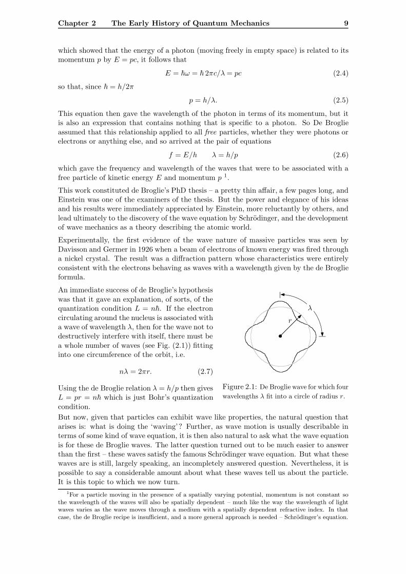
An immediate success of de Broglie’s hypothesiswas that it gave an explanation, of sorts, of thequantization condition L = n�. If the electroncirculating around the nucleus is associated witha wave of wavelength λ, then for the wave not todestructively interfere with itself, there must bea whole number of waves (see Fig. (2.1)) fittinginto one circumference of the orbit, i.e.
nλ = 2πr. (2.7)
Using the de Broglie relation λ = h/p then givesL = pr = n� which is just Bohr’s quantizationcondition.
r
λ
Figure 2.1: De Broglie wave for which fourwavelengths λ fit into a circle of radius r.
But now, given that particles can exhibit wave like properties, the natural question thatarises is: what is doing the ‘waving’? Further, as wave motion is usually describable interms of some kind of wave equation, it is then also natural to ask what the wave equationis for these de Broglie waves. The latter question turned out to be much easier to answerthan the first – these waves satisfy the famous Schrodinger wave equation. But what thesewaves are is still, largely speaking, an incompletely answered question. Nevertheless, it ispossible to say a considerable amount about what these waves tell us about the particle.It is this topic to which we now turn.
1For a particle moving in the presence of a spatially varying potential, momentum is not constant sothe wavelength of the waves will also be spatially dependent – much like the way the wavelength of lightwaves varies as the wave moves through a medium with a spatially dependent refractive index. In thatcase, the de Broglie recipe is insufficient, and a more general approach is needed – Schrodinger’s equation.
Chapter 3
The Wave Function
On the basis of the assumption that the de Broglie relations give the frequency and wave-length of some kind of wave to be associated with a particle, plus the assumption thatit makes sense to add together waves of different frequencies, it is possible to learn aconsiderable amount about these waves without actually knowing beforehand what theyrepresent. But studying different examples does provide some insight into what the ul-timate interpretation is, the so-called Born interpretation, which is that these waves are‘probability waves’ in the sense that the amplitude squared of the waves gives the prob-ability of observing (or detecting, or finding – a number of different terms are used) theparticle in some region in space. Hand-in-hand with this interpretation is the Heisenberguncertainty principle which, historically, preceded the formulation of the probability in-terpretation. From this principle, it is possible to obtain a number of fundamental resultseven before the full machinery of wave mechanics is in place.
In this Chapter, some of the consequences of de Broglie’s hypothesis of associating waveswith particles are explored, leading to the concept of the wave function, and its probabilityinterpretation.
3.1 The Harmonic Wave Function
On the basis of de Broglie’s hypothesis, there is associated with a particle of energy E andmomentum p, a wave of frequency f and wavelength λ given by the de Broglie relationsEq. (2.6). It more usual to work in terms of the angular frequency ω = 2πf and wavenumber k = 2π/λ so that the de Broglie relations become
ω = E/� k = p/�. (3.1)
With this in mind, and making use of what we already know about what the mathematicalform is for a wave, we are in a position to make a reasonable guess at a mathematicalexpression for the wave associated with the particle. The possibilities include (in onedimension)
Ψ(x, t) = A sin(kx− ωt), A cos(kx− ωt), Aei(kx−ωt), . . . (3.2)
At this stage, we have no idea what the quantity Ψ(x, t) represents physically. It is giventhe name the wave function, and in this particular case we will use the term harmonicwave function to describe any trigonometric wave function of the kind listed above. As
Chapter 3 The Wave Function 11
we will see later, in general it can take much more complicated forms than a simple singlefrequency wave, and is almost always a complex valued function.
In order to understand what information may be contained in the wave function, whichwill lead us to gaining a physical understanding of what it might represent, we will turnthings around briefly and look at what we can learn about the properties of a particle ifwe know what its wave function is.
First, given that the wave has frequency ω and wave number k, then it is straightforwardto calculate the phase velocity vp of the wave:
vp =ω
k=
�ω
�k=E
p=
12mv
2
mv= 1
2v. (3.3)
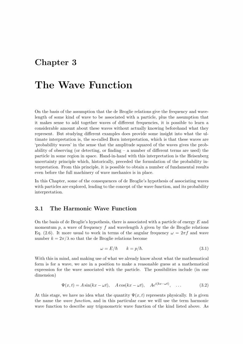
Thus, given the frequency and wave number of a wave function, we can determine thespeed of the particle from the phase velocity of its wave function, v = 2vp. We couldalso try to learn from the wave function the position of the particle. However, the wavefunction above tells us nothing about where the particle is to be found in space. Wecan make this statement because this wave function is the same everywhere i.e. there isnothing whatsoever to distinguish Ψ at one point in space from any other, see Fig. (3.1).
Ψ(x, t)
x
Figure 3.1: A wave function of constant amplitude and wavelength. The wave is the sameeverywhere and so there is no distinguishing feature that could indicate one possible position ofthe particle from any other.
Thus, this particular wave function gives no information on the whereabouts of the particlewith which it is associated. So from a harmonic wave function it is possible to learn howfast a particle is moving, but not what the position is of the particle.
3.2 Wave Packets
From what was said above about a wave function that was constant throughout all space,it would seem that a wave function can only convey information on the position of theparticle if the wave function did not have the same amplitude throughout all space. Infact, since what we mean by a particle is a physical object that is confined to a highlylocalized region in space, ideally a point, it would be intuitively appealing to be ableto devise a wave function that is zero or nearly so everywhere in space except for onelocalized region. It is in fact possible to construct, from the harmonic wave functions, awave function which has this property. To show how this is done, we first consider whathappens if we combine together two harmonic waves of very close frequency. The resultis well-known: a ‘beat note’ is produced, i.e. periodically in space the waves add togetherin phase to produce a local maximum, while midway in between the waves will be totallyout of phase and hence will destructively interfere. Each localized maximum is known
Chapter 3 The Wave Function 12
as a wave packet, so what is produced is a series of wave packets. Now suppose we addtogether a large number of harmonic waves with wave numbers k1, k2, k3, . . . all lying inthe range:
k −∆k < kn < k + ∆k (3.4)
around a mean value k, i.e.
Ψ(x, t) =A(k1) cos(k1x− ω1t) +A(k2) cos(k2x− ω2t) + . . .
=∑n
A(kn) cos(knx− ωnt) (3.5)
where A(k) is a function peaked about the mean value k with a full width at half maximumof 2∆k. (There is no significance to be attached to the use of cos functions here – theidea is simply to illustrate a point.) What is found is that in the limit in which the sumbecomes an integral:
Ψ(x, t) =∫ +∞
−∞A(k) cos(kx− ωt) dk (3.6)
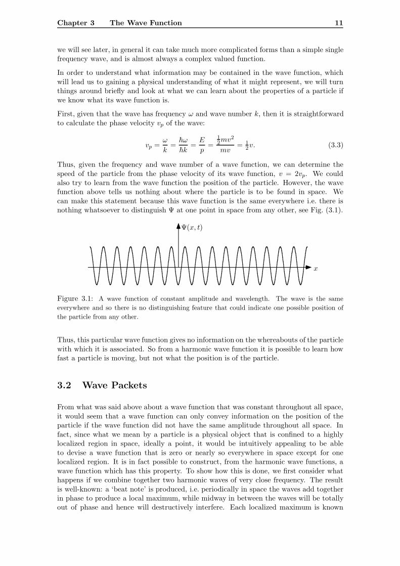
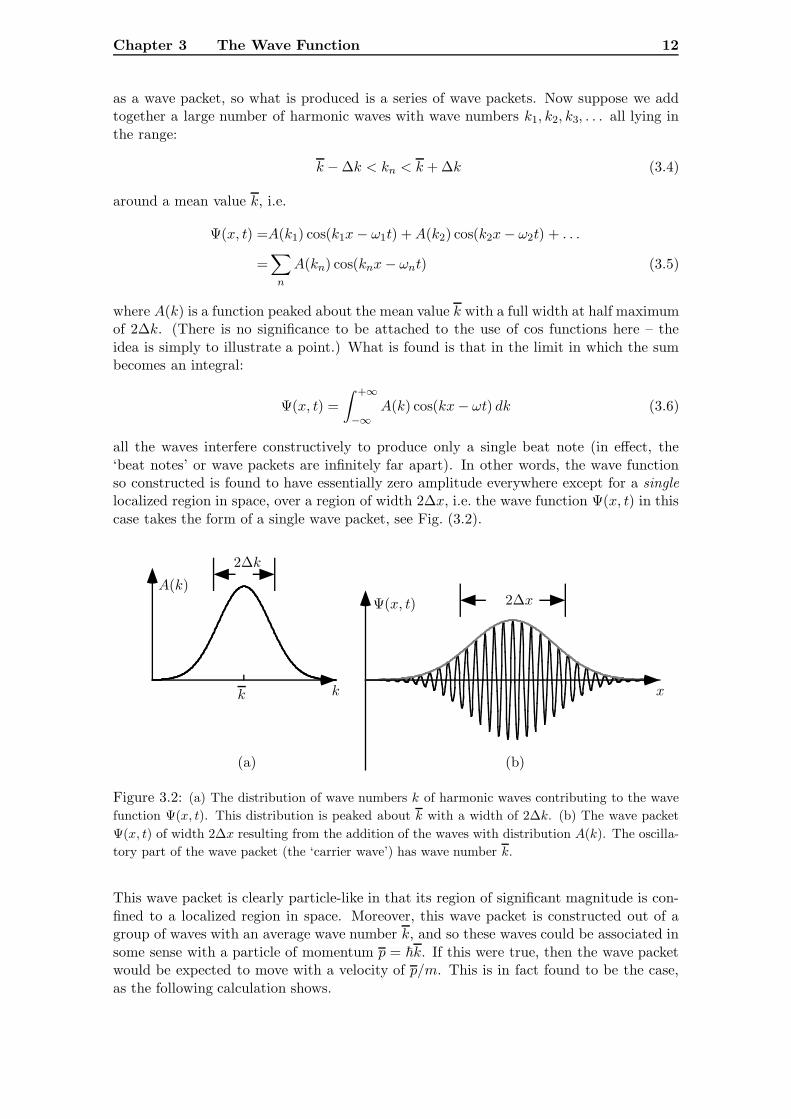
all the waves interfere constructively to produce only a single beat note (in effect, the‘beat notes’ or wave packets are infinitely far apart). In other words, the wave functionso constructed is found to have essentially zero amplitude everywhere except for a singlelocalized region in space, over a region of width 2∆x, i.e. the wave function Ψ(x, t) in thiscase takes the form of a single wave packet, see Fig. (3.2).
1'-1"
8"
(a) (b)
2∆k
2∆x
xkk
Ψ(x, t)A(k)
Figure 3.2: (a) The distribution of wave numbers k of harmonic waves contributing to the wavefunction Ψ(x, t). This distribution is peaked about k with a width of 2∆k. (b) The wave packetΨ(x, t) of width 2∆x resulting from the addition of the waves with distribution A(k). The oscilla-tory part of the wave packet (the ‘carrier wave’) has wave number k.
This wave packet is clearly particle-like in that its region of significant magnitude is con-fined to a localized region in space. Moreover, this wave packet is constructed out of agroup of waves with an average wave number k, and so these waves could be associated insome sense with a particle of momentum p = �k. If this were true, then the wave packetwould be expected to move with a velocity of p/m. This is in fact found to be the case,as the following calculation shows.
Chapter 3 The Wave Function 13
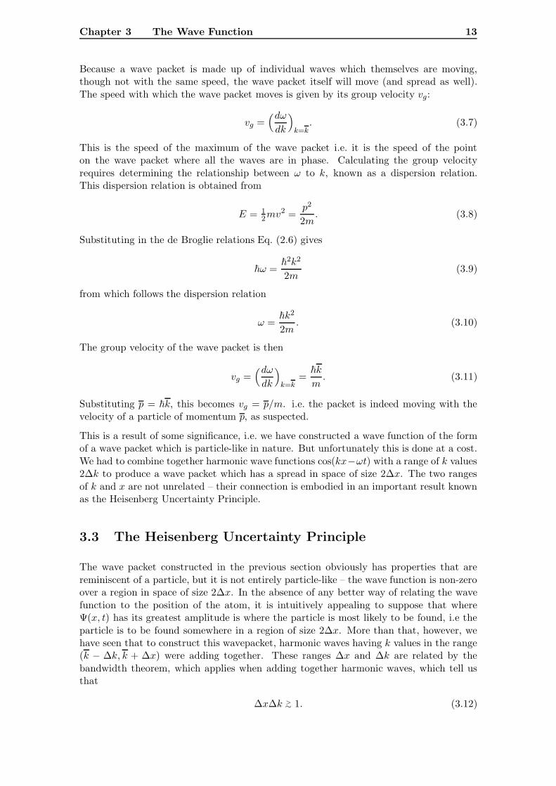
Because a wave packet is made up of individual waves which themselves are moving,though not with the same speed, the wave packet itself will move (and spread as well).The speed with which the wave packet moves is given by its group velocity vg:
vg =(dωdk
)k=k
. (3.7)
This is the speed of the maximum of the wave packet i.e. it is the speed of the pointon the wave packet where all the waves are in phase. Calculating the group velocityrequires determining the relationship between ω to k, known as a dispersion relation.This dispersion relation is obtained from
E = 12mv
2 =p2
2m. (3.8)
Substituting in the de Broglie relations Eq. (2.6) gives
�ω =�2k2
2m(3.9)
from which follows the dispersion relation
ω =�k2
2m. (3.10)
The group velocity of the wave packet is then
vg =(dωdk
)k=k
=�k
m. (3.11)
Substituting p = �k, this becomes vg = p/m. i.e. the packet is indeed moving with thevelocity of a particle of momentum p, as suspected.
This is a result of some significance, i.e. we have constructed a wave function of the formof a wave packet which is particle-like in nature. But unfortunately this is done at a cost.We had to combine together harmonic wave functions cos(kx−ωt) with a range of k values2∆k to produce a wave packet which has a spread in space of size 2∆x. The two rangesof k and x are not unrelated – their connection is embodied in an important result knownas the Heisenberg Uncertainty Principle.
3.3 The Heisenberg Uncertainty Principle
The wave packet constructed in the previous section obviously has properties that arereminiscent of a particle, but it is not entirely particle-like – the wave function is non-zeroover a region in space of size 2∆x. In the absence of any better way of relating the wavefunction to the position of the atom, it is intuitively appealing to suppose that whereΨ(x, t) has its greatest amplitude is where the particle is most likely to be found, i.e theparticle is to be found somewhere in a region of size 2∆x. More than that, however, wehave seen that to construct this wavepacket, harmonic waves having k values in the range(k − ∆k, k + ∆x) were adding together. These ranges ∆x and ∆k are related by thebandwidth theorem, which applies when adding together harmonic waves, which tell usthat
∆x∆k >∼ 1. (3.12)
Chapter 3 The Wave Function 14
Using p = �k, we have ∆p = �∆k so that
∆x∆p >∼ �. (3.13)
[A more rigorous derivation, based on a more precise definition of ∆x and ∆k leads to
∆x∆p ≥ 12� (3.14)
though we will mostly use the result Eq. (3.13).]
A closer look at this result is warranted. A wave packet that has a significant amplitudewithin a range 2∆x was constructed from harmonic wave functions which represent arange of momenta p − ∆p to p + ∆p. We can say then say that the particle is likelyto be found somewhere in the region 2∆x, and given that wave functions representing arange of possible momenta were used to form this wave packet, we could also say that themomentum of the particle will have a value in the range p−∆p to p+∆p. The quantities ∆xand ∆p are known as uncertainties for reasons that will become increasingly apparent,and the relation above Eq. (3.14) is known as the Heisenberg uncertainty relation forposition and momentum. It tells us that we cannot determine, from knowledge of thewave function alone, the exact position and momentum of a particle at the same time.In the extreme case that ∆x = 0, then the position uncertainty is zero, but Eq. (3.14)tells us that the uncertainty on the momentum is infinite, i.e. the momentum is entirelyunknown. A similar statement applies if ∆p = 0.
This conclusion flies in the face of our experience in the macroscopic world, namely thatthere is no problem, in principle, with knowing the position and momentum of a particle.Thus, we could then argue that more information is needed, i.e. that a prescription isstill to be found that will ultimately enable us to find the position and the momentum ofthe particle from the wave function, or, in other words, that the wave function does notgive complete information on the state of the particle. Einstein fought vigorously for thisposition. In a famous series of exchanges with Neils Bohr and others, he argued that thewave function was not a complete description of ‘reality’, and that there was somewhere,in some sense, a repository of missing information that will remove the incompleteness ofthe wave function – somewhat later termed ‘hidden variables’. Unfortunately (for thosewho hold to his point of view) evidence has mounted, particularly in the past few decades,that the wave function (or its analogues in the more general formulation of quantummechanics) does indeed represent the full picture – the most that can ever be knownabout a particle is what can be learned from its wave function. This means that thedifficulty encountered above concerning not being able, in general, to exactly pinpointboth the position or the momentum of a particle from knowledge of its wave function isan irreducible property of the natural world. It is only at the macroscopic level wherethe uncertainties mentioned above become so small as to be experimentally unmeasurablethat the effects of the uncertainty principle have no apparent effect.
3.3.1 The Size of an Atom
One important application of the uncertainty relation is to do with determining the sizeof atoms. Recall that classically atoms should not exist: the electrons must spiral intothe nucleus, radiating away their excess energy as they do. However, if this were thecase, then the situation would be arrived at in which the position and the momentum ofthe electrons would be known: stationary, and at the position of the nucleus. This is inconflict with the uncertainty principle, so it must be the case that the electron can spiralinward no further than an amount that is consistent with the uncertainty principle.
Chapter 3 The Wave Function 15
To see what the uncertainty principle does tell us, consider the simplest example: ahydrogen atom. Here the electron is trapped in the Coulomb potential well due to thepositive nucleus. We can then argue that if the electron cannot have a precisely definedposition, then suppose that it is confined to a spherical (by symmetry) shell of radius a.Thus, the uncertainty ∆x in x will be a, and similarly for the y and z positions. But,when moving within this region, px, the x component of momentum, will, by symmetry,swing between two equal and opposite values, p and −p say, and hence px will have anuncertainty of ∆px ≈ 2p. By appealing to symmetry once again, the y and z componentsof momentum can be seen to have the same uncertainty.
By the uncertainty principle ∆px∆x ≈ �, (and similarly for the other two components),the uncertainty in the x component of momentum will then be ∆px ≈ �/a, and hencep ≈ �/a. The kinetic energy of the particle will then be
T =p2
2m≈ �2
2ma2(3.15)
so including the Coulomb potential energy, the total energy of the particle will be
E ≈ �2
2ma2− e2
4πε0a. (3.16)
The lowest possible energy of the atom is then obtained by simple differential calculus.Thus, taking the derivative of E with respect to a and equating this to zero and solvingfor a gives
a ≈ 4πε0�2
me2≈ 0.5 nm (3.17)
and the minimum energy
Emin ≈− 12
me4
(4πε0)2�2(3.18)
≈− 13.6 eV. (3.19)
The above values for atomic size and atomic energies are what are observed in practice.The uncertainty relation has yielded considerable information on atomic structure withoutknowing all that much about what a wave function is supposed to represent!
The exactness of the above result is somewhat fortuitous, but the principle is neverthelesscorrect: the uncertainty principle demands that there be a minimum size to an atom. Ifa hydrogen atom has an energy above this minimum, it is free to radiate away energy byemission of electromagnetic energy (light) until it reaches this minimum. Beyond that, itcannot radiate any more energy. Classical EM theory says that it should, but it does not.The conclusion is that there must also be something amiss with classical EM theory, whichin fact turns out to be the case: the EM field too must treated quantum mechanically.When this is done, there is consistency between the demands of quantum EM theory andthe quantum structure of atoms – an atom in its lowest energy level (the ground state)cannot, in fact, radiate – the ground state of an atom is stable.
Another important situation for which the uncertainty principle gives a surprising amountof information is that of the harmonic oscillator.
Chapter 3 The Wave Function 16
3.3.2 The Minimum Energy of a Simple Harmonic Oscillator
By using Heisenberg’s uncertainty principle in the form ∆x∆p ≈ �, it is also possible toestimate the lowest possible energy level (ground state) of a simple harmonic oscillator.The simple harmonic oscillator potential is given by
U =12µx2 (3.20)
This is a particularly important example as the simple harmonic oscillator potential isfound to arise in a wide variety of circumstaces such as an electron trapped in a wellbetween two nuclei, or the oscillations of a linear molecule, or indeed, the lowest energyof a single mode quantum mechanical electromagnetic field.
We start by assuming that in the lowest energy level, the oscillations of the particle havean amplitude of a, so that the oscillations swing between −a and a. We further assumethat the momentum of the particle can vary between p and −p. Consequently, we canassign an uncertainty ∆x = a in the position of the particle, and an uncertainty ∆p = p inthe momentum of the particle. These two uncertainties will be related by the uncertaintyrelation
∆x∆p ≈ � (3.21)
from which we conclude that
p ≈ �/a. (3.22)
The total energy of the oscillator is
E =p2
2m+ 1
2µx2 (3.23)
so that roughly, if a is the amplitude of the oscillation, and p ≈ �/a is the maximummomentum of the particle then
E ≈ 12
(1
2m�
2
a2+ 1
2µa2
)(3.24)
where the extra factor of 12 is included to take account of the fact that the kinetic and
potential energy terms are each their maximum possible values.
The minimum value of E can be found using differential calculus i.e.
dE
da= 1
2
(− 1m
�2
a3+ µa
)= 0. (3.25)
Solving for a gives
a2 =�√mµ
. (3.26)
Substituting this into the expression for E then gives for the minimum energy
Emin ≈ 12�
õ
m. (3.27)
In terms of the natural frequency ω =√µ/m we have
Emin ≈ 12�ω. (3.28)
Chapter 3 The Wave Function 17
A more precise quantum mechanical calculation shows that this result is (fortuitously)exactly correct, i.e. the ground state of the harmonic oscillator has a non-zero energy of12�ω.
It was Heisenberg’s discovery of the uncertainty relation, and various other real and imag-ined experiments that ultimately lead to a fundamental proposal (by Max Born) concern-ing the physical meaning of the wave function. We shall arrive at this interpretation byway of the famous two slit interference experiment.
Chapter 4
The Two Slit Experiment
This experiment is said to illustrate the essential mystery of quantum mechanics. It willbe considered in three forms: performed with macroscopic particles, with waves, andwith electrons. The first two merely show what we expect to see based on our everydayexperience. It is the third which displays the counterintuitive behaviour of microscopicsystems – a peculiar combination of particle and wave like behaviour which cannot beunderstood in terms of the concepts of classical physics, and which implies the existenceof a new set of laws, expressed in a new mathematical language, in terms of which thebehaviour of such systems can be described and in some sense ‘understood’. The analysisof the two slit experiment presented below is more or less taken from Volume III of theFeynman Lectures in Physics.
4.1 An Experiment with Bullets
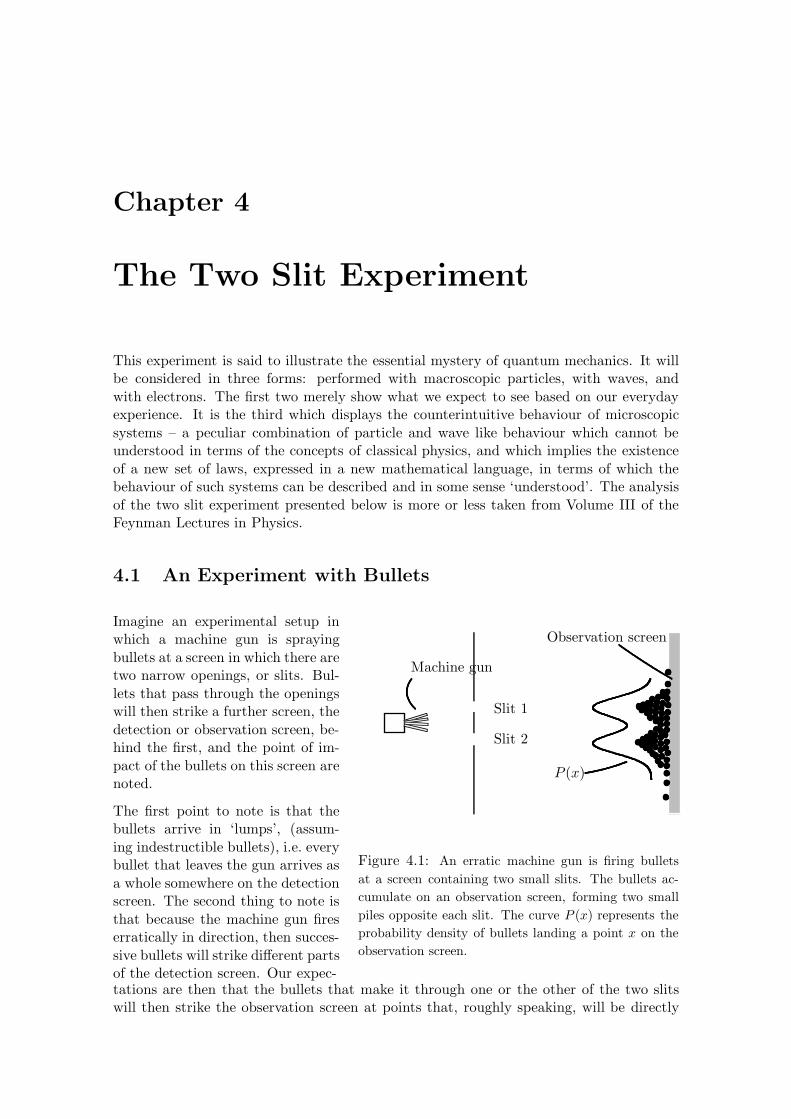
Imagine an experimental setup inwhich a machine gun is sprayingbullets at a screen in which there aretwo narrow openings, or slits. Bul-lets that pass through the openingswill then strike a further screen, thedetection or observation screen, be-hind the first, and the point of im-pact of the bullets on this screen arenoted.
The first point to note is that thebullets arrive in ‘lumps’, (assum-ing indestructible bullets), i.e. everybullet that leaves the gun arrives asa whole somewhere on the detectionscreen. The second thing to note isthat because the machine gun fireserratically in direction, then succes-sive bullets will strike different partsof the detection screen. Our expec-
Machine gun
Slit 1
Slit 2
Observation screen
P (x)
Figure 4.1: An erratic machine gun is firing bulletsat a screen containing two small slits. The bullets ac-cumulate on an observation screen, forming two smallpiles opposite each slit. The curve P (x) represents theprobability density of bullets landing a point x on theobservation screen.
tations are then that the bullets that make it through one or the other of the two slitswill then strike the observation screen at points that, roughly speaking, will be directly
Chapter 4 The Two Slit Experiment 19
aligned with the slits, and so will accummulate in two ‘piles’, as indicated in Fig. (4.1).
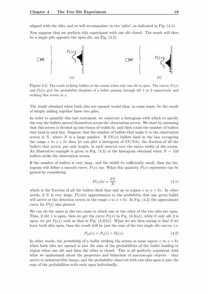
Now suppose that we perform this experiment with one slit closed. The result will thenbe a single pile opposite the open slit, see Fig. (4.2).
(a) (b)
P1(x)
P2(x)
Figure 4.2: The result of firing bullets at the screen when only one slit is open. The curves P1(x)and P2(x) give the probability densities of a bullet passing through slit 1 or 2 respectively andstriking ther screen at x.
The result obtained when both slits are opened would then, in some sense, be the resultof simply adding together these two piles.
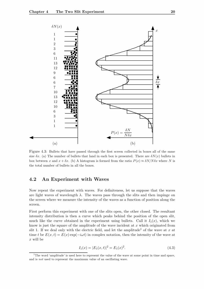
In order to quantify this last statement, we construct a histogram with which to specifythe way the bullets spread themselves across the observation screen. We start by assumingthat this screen is divided up into boxes of width δx, and then count the number of bulletsthat land in each box. Suppose that the number of bullets that make it to the observationscreen is N , where N is a large number. If δN (x) bullets land in the box occupyingthe range x to x + δx then we can plot a histogram of δN/Nδx, the fraction of all thebullets that arrive, per unit length, in each interval over the entire width of the screen.An illustrative example is given in Fig. (4.3) of the histogram obtained when N = 133bullets strike the observation screen.
If the number of bullets is very large, and the width δx sufficiently small, then the his-togram will define a smooth curve, P (x) say. What this quantity P (x) represents can begained by considering
P (x)δx =δN
N(4.1)
which is the fraction of all the bullets fired that end up in region x to x + δx. In otherwords, if N is very large, P (x)δx approximates to the probability that any given bulletwill arrive at the detection screen in the range x to x+ δx. In Fig. (4.3) the approximatecurve for P (x) also plotted.
We can do the same in the two cases in which one or the other of the two slits are open.Thus, if slit 1 is open, then we get the curve P1(x) in Fig. (4.3(a)), while if only slit 2 isopen, we get P2(x) such as that in Fig. (4.3(b)). What we are then saying is that if weleave both slits open, then the result will be just the sum of the two single slit curves, i.e.
P12(x) = P1(x) + P2(x). (4.2)
In other words, the probability of a bullet striking the screen in some region x to x + δxwhen both slits are opened is just the sum of the probabilities of the bullet landing inregion when one slit and then the other is closed. This is all perfectly consistent withwhat we understand about the properties and behaviour of macroscopic objects – theyarrive in indestructible lumps, and the probability observed with two slits open is just thesum of the probabilities with each open individually.
Chapter 4 The Two Slit Experiment 20
P (x) =δN
Nδx
x
δx
δN (x)
112361113129667101312106311
(a) (b)
Figure 4.3: Bullets that have passed through the first screen collected in boxes all of the samesize δx. (a) The number of bullets that land in each box is presented. There are δN(x) bullets inbox between x and x+ δx. (b) A histogram is formed from the ratio P (x) ≈ δN/Nδx where N isthe total number of bullets in all the boxes.
4.2 An Experiment with Waves
Now repeat the experiment with waves. For definiteness, let us suppose that the wavesare light waves of wavelength λ. The waves pass through the slits and then impinge onthe screen where we measure the intensity of the waves as a function of position along thescreen.
First perform this experiment with one of the slits open, the other closed. The resultantintensity distribution is then a curve which peaks behind the position of the open slit,much like the curve obtained in the experiment using bullets. Call it I1(x), which weknow is just the square of the amplitude of the wave incident at x which originated fromslit 1. If we deal only with the electric field, and let the amplitude1 of the wave at x attime t be E(x, t) = E(x) exp(−iωt) in complex notation, then the intensity of the wave atx will be
I1(x) = |E1(x, t)|2 = E1(x)2. (4.3)
1The word ‘amplitude’ is used here to represent the value of the wave at some point in time and space,and is not used to represent the maximum value of an oscillating wave.
Chapter 4 The Two Slit Experiment 21
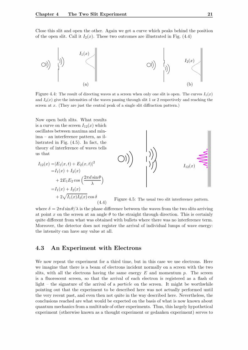
Close this slit and open the other. Again we get a curve which peaks behind the positionof the open slit. Call it I2(x). These two outcomes are illustrated in Fig. (4.4)
(a) (b)
I1(x)
I2(x)
Figure 4.4: The result of directing waves at a screen when only one slit is open. The curves I1(x)and I2(x) give the intensities of the waves passing through slit 1 or 2 respectively and reaching thescreen at x. (They are just the central peak of a single slit diffraction pattern.)
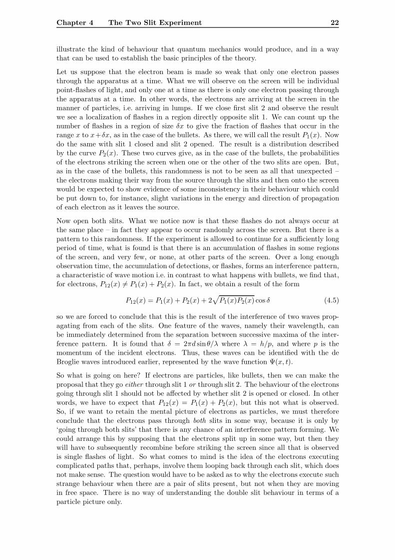
Now open both slits. What resultsis a curve on the screen I12(x) whichoscillates between maxima and min-ima – an interference pattern, as il-lustrated in Fig. (4.5). In fact, thetheory of interference of waves tellsus that
I12(x) =|E1(x, t) +E2(x, t)|2
=I1(x) + I2(x)
+ 2E1E2 cos(2πd sinθ
λ
)=I1(x) + I2(x)
+ 2√I1(x)I2(x) cos δ
(4.4)
I12(x)
Figure 4.5: The usual two slit interference pattern.
where δ = 2πd sinθ/λ is the phase difference between the waves from the two slits arrivingat point x on the screen at an angle θ to the straight through direction. This is certainlyquite different from what was obtained with bullets where there was no interference term.Moreover, the detector does not register the arrival of individual lumps of wave energy:the intensity can have any value at all.
4.3 An Experiment with Electrons
We now repeat the experiment for a third time, but in this case we use electrons. Herewe imagine that there is a beam of electrons incident normally on a screen with the twoslits, with all the electrons having the same energy E and momentum p. The screenis a fluorescent screen, so that the arrival of each electron is registered as a flash oflight – the signature of the arrival of a particle on the screen. It might be worthwhilepointing out that the experiment to be described here was not actually performed untilthe very recent past, and even then not quite in the way described here. Nevertheless, theconclusions reached are what would be expected on the basis of what is now known aboutquantum mechanics from a multitude of other experiments. Thus, this largely hypotheticalexperiment (otherwise known as a thought experiment or gedanken experiment) serves to
Chapter 4 The Two Slit Experiment 22
illustrate the kind of behaviour that quantum mechanics would produce, and in a waythat can be used to establish the basic principles of the theory.
Let us suppose that the electron beam is made so weak that only one electron passesthrough the apparatus at a time. What we will observe on the screen will be individualpoint-flashes of light, and only one at a time as there is only one electron passing throughthe apparatus at a time. In other words, the electrons are arriving at the screen in themanner of particles, i.e. arriving in lumps. If we close first slit 2 and observe the resultwe see a localization of flashes in a region directly opposite slit 1. We can count up thenumber of flashes in a region of size δx to give the fraction of flashes that occur in therange x to x+δx, as in the case of the bullets. As there, we will call the result P1(x). Nowdo the same with slit 1 closed and slit 2 opened. The result is a distribution describedby the curve P2(x). These two curves give, as in the case of the bullets, the probabilitiesof the electrons striking the screen when one or the other of the two slits are open. But,as in the case of the bullets, this randomness is not to be seen as all that unexpected –the electrons making their way from the source through the slits and then onto the screenwould be expected to show evidence of some inconsistency in their behaviour which couldbe put down to, for instance, slight variations in the energy and direction of propagationof each electron as it leaves the source.
Now open both slits. What we notice now is that these flashes do not always occur atthe same place – in fact they appear to occur randomly across the screen. But there is apattern to this randomness. If the experiment is allowed to continue for a sufficiently longperiod of time, what is found is that there is an accumulation of flashes in some regionsof the screen, and very few, or none, at other parts of the screen. Over a long enoughobservation time, the accumulation of detections, or flashes, forms an interference pattern,a characteristic of wave motion i.e. in contrast to what happens with bullets, we find that,for electrons, P12(x) �= P1(x) + P2(x). In fact, we obtain a result of the form
P12(x) = P1(x) + P2(x) + 2√P1(x)P2(x) cos δ (4.5)
so we are forced to conclude that this is the result of the interference of two waves prop-agating from each of the slits. One feature of the waves, namely their wavelength, canbe immediately determined from the separation between successive maxima of the inter-ference pattern. It is found that δ = 2πd sinθ/λ where λ = h/p, and where p is themomentum of the incident electrons. Thus, these waves can be identified with the deBroglie waves introduced earlier, represented by the wave function Ψ(x, t).
So what is going on here? If electrons are particles, like bullets, then we can make theproposal that they go either through slit 1 or through slit 2. The behaviour of the electronsgoing through slit 1 should not be affected by whether slit 2 is opened or closed. In otherwords, we have to expect that P12(x) = P1(x) + P2(x), but this not what is observed.So, if we want to retain the mental picture of electrons as particles, we must thereforeconclude that the electrons pass through both slits in some way, because it is only by‘going through both slits’ that there is any chance of an interference pattern forming. Wecould arrange this by supposing that the electrons split up in some way, but then theywill have to subsequently recombine before striking the screen since all that is observedis single flashes of light. So what comes to mind is the idea of the electrons executingcomplicated paths that, perhaps, involve them looping back through each slit, which doesnot make sense. The question would have to be asked as to why the electrons execute suchstrange behaviour when there are a pair of slits present, but not when they are movingin free space. There is no way of understanding the double slit behaviour in terms of aparticle picture only.
Chapter 4 The Two Slit Experiment 23
We may argue that one way of resolving the issue is to actually monitor the slits, andlook to see when an electron passes through each slit. This could be done, for instance, byshining a light on each of the slits. If an electron goes through a slit, then it scatters someof this light, which can be observed with a microscope. We immediately know what slit theelectron passed through, but unfortunately, as a consequence of gaining this knowledge,what is found is that the interference pattern disappears, and what is seen on the screenis the same result as for bullets. Thus, by monitoring an explicitly particle characteristicof the electron, i.e. where it is, the experiment yields the results that would be found withparticles. A close analysis of this shows that the effect of the light is to produce a recoil inthe motion of any electron that is observed. The amount of deflection is itself random, butin general its effect is to displace an electron so that one that was, for instance, headingfor a maximum of the interference pattern, could now strike the screen at the position ofa minimum. The overall result is to wipe out the interference pattern. In fact, as far aswe know any experiment that can be devised – either a real experiment or a gedankenexperiment – that attempts to determine which slit the electron passes through alwaysresults in the disappearance of the interference pattern. The details of the way the physicsconspires to produce this result differs from one experiment to the other, but the final resultis the same: if we know which slit the electron goes through, then the observed pattern ofthe screen is the same as found with bullets: no interference, with P12(x) = P1(x) +P2(x).Confirming that the electrons definitely go through one slit or another, which is a propertythat we expect particles to possess, then results in the electrons behaving as particles do.If we do not look, then in some sense each electron passes through both slits, resulting inthe formation of an interference pattern, the signature of wave motion. Thus, the electronsbehave either like particles or like waves, depending on what it is that is being observed,a dichotomy that is known as wave-particle duality.
There is therefore a deep physical principle at play here that overrides any attempt to bothwatch where the particles are, and to observe the interference effects. The principle is theuncertainty principle. It can be argued that pinning down the position of an electron to bepassing through a particular slit amounts to specifying its x position to within ∆x ≈ d/2,where d is the separation of the slits. But doing so implies that there is an uncertainty inthe sideways momentum of the electron given by ∆px ≈ 2�/d. Since the electrons have atotal momentum p, this amounts to a change in direction through an angle
∆θ =∆pxp≈ λ
πd(4.6)
Since the angular separation between a minimum and a neighbouring maximum of thediffraction pattern is λ/2d, it is clear that the uncertainty in the sideways momentumarising from trying to observe through which slit the particle passes is enough to displacea particle from a maximum into a neighbouring minimum, washing out the interferencepattern.
4.4 Probability Amplitudes
First, a summary of what has been seen so far. In the case of waves, we have seen thatthe total amplitude of the waves incident on the screen at the point x is given by
E(x, t) = E1(x, t) +E2(x, t) (4.7)
Chapter 4 The Two Slit Experiment 24
where E1(x, t) and E2(x, t) are the waves arriving at the point x from slits 1 and 2respectively. The intensity of the resultant interference pattern is then given by
I12(x) =|E(x, t)|2
=|E1(x, t) + E2(x, t)|2
=I1(x) + I2(x) + 2E1E2 cos(2πd sinθ
λ
)=I1(x) + I2(x) + 2
√I1(x)I2(x) cos δ (4.8)
where δ = 2πd sinθ/λ is the phase difference between the waves arriving at the point xfrom slits 1 and 2 respectively, at an angle θ to the straight through direction.
The point was then made that the probability density for an electron to arrive at theobservation screen at point x had the same form, i.e. it was given by the same mathematicalexpression
P12(x) = P1(x) + P2(x) + 2√P1(x)P2(x) cos δ. (4.9)
so we were forced to conclude that this is the result of the interference of two wavespropagating from each of the slits. Moreover, the wavelength of these waves was foundto be given by λ = h/p, where p is the momentum of the incident electrons so that thesewaves can be identified with the de Broglie waves introduced earlier, represented by thewave function Ψ(x, t).
Thus, we are proposing that incident on the observation screen is the de Broglie waveassociated with each electron whose total amplitude at point x is given by
Ψ(x, t) = Ψ1(x, t) + Ψ2(x, t) (4.10)
where Ψ1(x, t) and Ψ2(x, t) are the amplitudes at x of the waves emanating from slits 1and 2 respectively. Further, since P12(x)δx is the probability of an electron being detectedin the region x, x+ δx, we are proposing that
|Ψ(x, t)|2δx ∝ probability of observing an electron in x, x+ δx (4.11)
so that we can interpret Ψ(x, t) as a probability amplitude. This is the famous probabilityinterpretation of the wave function first proposed by Born on the basis of his own obser-vations of the outcomes of scattering experiments, as well as awareness of Einstein’s owninclinations along these lines. Somewhat later, after proposing his uncertainty relation,Heisenberg made a similar proposal.
There are two other important features of this result that are worth taking note of:
• If the detection event can arise in two different ways (i.e. electron detected afterhaving passed through either slit 1 or 2) and the two possibilities remain unobserved,then the total probability of detection is
P = |Ψ1 + Ψ2|2 (4.12)
i.e. we add the amplitudes and then square the result.
• If the experiment contains a part that even in principle can yield information onwhich of the alternate paths were followed, then
P = P1 + P2 (4.13)
i.e. we add the probabilities associated with each path.
Chapter 4 The Two Slit Experiment 25
What this last point is saying, for example in the context of the two slit experiment, is that,as part of the experimental set-up, there is equipment that is monitoring through whichslit the particle goes. Even if this equipment is automated, and simply records the result,say in some computer memory, and we do not even bother to look the results, the fact thatthey are still available means that we should add the probabilities. This last point can beunderstood if we view the process of observation of which path as introducing randomnessin such a manner that the interference effects embodied in the cos δ are smeared out. Inother words, the cos δ factor – which can range between plus and minus one – will averageout to zero, leaving behind the sum of probability terms.
4.5 The Fundamental Nature of Quantum Probability
The fact that the results of the experiment performed with electrons yields outcomeswhich appear to vary in a random way from experiment to experiment at first appearsto be identical to the sort of randomness that occurs in the experiment performed withthe machine gun. In the latter case, the random behaviour can be explained by the factthat the machine gun is not a very well constructed device: it sprays bullets all over theplace. This seems to suggest that simply by refining the equipment,the randomness canbe reduced, in principle removing it all together if we are clever enough. At least, thatis what classical physics would lead us to believe. Classical physics permits unlimitedaccuracy in the fixing the values of physical or dynamical quantities, and our failure tolive up to this is simply a fault of inadequacies in our experimental technique.
However, the kind of randomness found in the case of the experiment performed withelectrons is of a different kind. It is intrinsic to the physical system itself. We are unableto refine the experiment in such a way that we can know precisely what is going on.Any attempt to do so gives rise to unpredictable changes, via the uncertainty principle.Put another way, it is found that experiments on atomic scale systems (and possiblyat macroscopic scales as well) performed under identical conditions, where everything isas precisely determined as possible, will always, in general, yield results that vary in arandom way from one run of the experiment to the next. This randomness is irreducible,an intrinsic part of the physical nature of the universe.
Attempts to remove this randomness by proposing the existence of so-called ‘classical hid-den variables’ have been made in the past. These variables are supposed to be classicalin nature – we are simply unable to determine their values, or control them in any way,and hence give rise to the apparent random behaviour of physical systems. Experimentshave been performed that test this idea, in which a certain inequality known as the Bellinequality, was tested. If these classical hidden variables did in fact exist, then the in-equality would be satisfied. A number of experiments have yielded results that are clearlyinconsistent with the inequality, so we are faced with having to accept that the physicsof the natural world is intrinsically random at a fundamental level, and in a way that isnot explainable classically, and that physical theories can do no more than predict theprobabilities of the outcome of any measurement.
Chapter 5
Wave Mechanics
The version of quantum mechanics based on studying the properties of the wave functionis known as wave mechanics, and is the version that first found favour amongst earlyresearchers in the quantum theory, in part because it involved setting up and solving apartial differential equation for the wave function, the famous Schrodinger equation, whichwas of a well-known and much studied form. As well as working in familiar mathematicalterritory, physicists and chemists were also working with something concrete in what wasin other ways a very abstract theory – the wave function was apparently a wave in spacewhich could be visualized, at least to a certain extent. But it must be borne in mind thatthe wave function is not an objectively real entity – it turns out that it is no more thanone aspect of a more general theory, quantum theory, that is convenient for certain classesof problems, and entirely inappropriate (or indeed inapplicable) to others1. Nevertheless,wave mechanics offers a fairly direct route to some of the more important features ofquantum mechanics, and for that reason, some attention is given here to some aspectsof wave mechanics prior to moving on, in later chapters, to considering the more generaltheory.
5.1 The Probability Interpretation of the Wave Function
The probability interpretation of the wave function was introduced in the preceding Chap-ter. It is restated here for convenience: if a particle is described by a wave function ψ(x, t),then
|Ψ(x, t)|2δx = Probability of observing the particle in the region (x, x+ δx) at time t.
Some obvious results follow immediately from this statement, one of the first being therequirement that the wave function be normalized to unity for all time:∫ +∞
−∞|Ψ(x, t)|2 dx = 1. (5.1)
1The wave function appears to be a wave in real space for a single particle, but that is only becauseit depends on x and t, in the same way as, say, the amplitude of a wave on a string can be written as afunction of x and t. But, for a system of more than one particle, the wave function becomes a functionof two space variables x1 and x2 say, as well as t: Ψ(x1, x2, t). It then makes no sense to talk about thevalue of the wave function at some position in space. In fact, the wave function is a wave that ‘exists’ inan abstract space known as phase space.
Chapter 5 Wave Mechanics 27
This condition on the wave function follows directly from the fact that the particle mustbe somewhere, so the total probability of finding it anywhere in space must add up tounity.
An immediate consequence of this condition is that the wave function must vanish asx → ±∞ otherwise the integral will have no hope of being finite. This condition on thewave function is found to lead to one of the most important results of quantum mechanics,namely that the energy of the particle (and other observable quantities as well) is quantized,that is to say, it can only have certain discrete values in circumstances in which, classically,the energy can have any value.
We can note at this stage that the wave function that we have been mostly dealing with,the wave function of a free particle of given energy and momentum
Ψ(x, t) = A sin(kx− ωt), A cos(kx− ωt), Aei(kx−ωt), . . . , (5.2)
does not satisfy the normalization condition Eq. (5.1) – the integral of |Ψ(x, t)|2 is infinite.Thus it already appears that there is an inconsistency in what we have been doing. How-ever, there is a place for such wave functions in the greater scheme of things, though thisis an issue that cannot be considered here. It is sufficient to interpret this wave function assaying that because it has the same amplitude everywhere in space, the particle is equallylikely to be found anywhere.
Finally we note that provided the wave function is normalized to unity, the probability offinding the particle over a finite region of space, say a < x < b, will be given by∫ b
a
|Ψ(x, t)|2 dx. (5.3)
5.2 Expectation Values and Uncertainties
Since |Ψ(x, t)|2 is a normalized probability density for the particle to be found in someregion in space, it can be used to calculate various statistical properties of the position ofthe particle. In defining these quantities, we must make use of the notion of an ‘ensembleof identically prepared systems’. By this we mean that we imagine that we set up anexperimental apparatus and use it to prepare an extremely large number N of particlesall in the same state. We then propose to measure the position of each particle at sometime t after the start of the preparation procedure. Presumably, because each particle hasgone through exactly the same preparation, they will all be in the same state at time t, asgiven by the wave function Ψ(x, t). The collection of particles is known as an ensemble,and it is common practice (and a point of contention) in quantum mechanics to refer tothe wave function as the wave function of the ensemble, rather than the wave function ofeach individual particle, though we will not consistently adopt this point-of-view.
When we measure the position of the particle at this time t, we will get a scatter of results,with a probability distribution given by P (x, t) = |Ψ(x, t)|2. Suppose we divide the rangeof x values into regions of width δx, and measure the number of particles for which thevalue of x lies in the range (x, x + δx), δN (x) say. The fraction of particles that areobserved to lie in this range will then be
δN (x)N
≈ P (x, t)δx (5.4)
Chapter 5 Wave Mechanics 28
where the approximate equality will become more exact as the number opf particles be-comes larger. We can then calculate the average value of all these results in the usual way,i.e.
〈x(t)〉 =∑
All δx
xδN (x)N
≈∑
All δx
xP (x, t)δx. (5.5)
In the limit in which the number of particles becomes infinitely large, and as δx→ 0, thisbecomes an integral:
〈x(t)〉 =∫ +∞
−∞xP (x, t) dx =
∫ +∞
−∞x |Ψ(x, t)|2dx (5.6)
i.e. this is the average value of, in effect, an infinite number of measurements of the positionof the particles all prepared in the same state described by the wave function Ψ(x, t). It isusually referred to as the expectation value of x. Similarly, expectation values of functionsof x can be derived. For f(x), we have
〈f(x)〉 =∫ +∞
−∞f(x) |Ψ(x, t)|2dx. (5.7)
In particular, we have
〈x2〉 =∫ +∞
−∞x2 |Ψ(x, t)|2dx. (5.8)
We can now define the uncertainty in the position of the particle by the usual statisticalquantity, the standard deviation (∆x)2, given by
(∆x)2 = 〈x2〉 − 〈x〉2. (5.9)
In order to illustrate the sort of results that can be obtained from the wave function, wewill consider a particularly simple example about which much can be said, even with thelimited understanding that we have at this stage. The model is that of a particle in aninfinitely deep potential well.
5.3 Particle in an Infinite Potential Well
Suppose we have a single particle of mass m confined to within a region 0 < x < L withpotential energy V = 0 bounded by infinitely high potential barriers, i.e. V =∞ for x < 0and x > L. This simple model is sufficient to describe (in one dimension), for instance,the properties of the conduction electrons in a metal (in the so-called free electron model),or the properties of gas particles in an ideal gas where the particles do not interact witheach other. We want to learn as much about the properties of the particle using what wehave learned about the wave function above.
The first point to note is that, because of the infinitely high barriers, the particle cannotbe found in the regions x > L and x < 0. Consequently, the wave function has to be zeroin these regions. If we make the not unreasonable assumption that the wave function hasto be continuous, then we must conclude that
Ψ(0, t) = Ψ(L, t) = 0. (5.10)
These conditions on Ψ(x, t) are known as boundary conditions.
Chapter 5 Wave Mechanics 29
Between the barriers, the energy of the particle is purely kinetic. Suppose the energy ofthe particle is E, so that
E =p2
2m. (5.11)
Using the de Broglie relation E = �k we then have that
k = ±√
2mE�
(5.12)
while, from E = �ω we have
ω = E/�. (5.13)
In the region 0 < x < L the particle is free, so the wave function must be of the formEq. (5.2), or perhaps a combination of such wave functions, in the manner that gave usthe wave packets in Section 3.2. In deciding on the possible form for the wave function,we are restricted by two requirements. First, the boundary conditions Eq. (5.10) mustbe satisfied and secondly, we note that the wave function must be normalized to unity,Eq. (5.1). The first of these conditions immediately implies that the wave function cannotbe simply A sin(kx− ωt), A cos(kx − ωt), or Aei(kx−ωt) or so on, as none of these will bezero at x = 0 and x = L for all time. The next step is therefore to try a combination ofthese wave functions. In doing so we note two things: first, from Eq. (5.12) we see thereare two possible values for k, and further we note that any sin or cos function can bewritten as a sum of complex exponentials:
cos θ =eiθ + e−iθ
2sin θ =
eiθ − e−iθ2i
which suggests that we can try combining the lot together and see if the two conditionsabove pick out the combination that works. Thus, we will try
Ψ(x, t) = Aei(kx−ωt) +Be−i(kx−ωt) +Cei(kx+ωt) +De−i(kx+ωt) (5.14)
where A, B, C, and D are coefficients that we wish to determine from the boundaryconditions and from the requirement that the wave function be normalized to unity for alltime.
First, consider the boundary condition at x = 0. Here, we must have
Ψ(0, t) = Ae−iωt + Beiωt +Ceiωt + De−iωt
= (A+D)e−iωt + (B + C)eiωt
= 0.
(5.15)
This must hold true for all time, which can only be the case if A+D = 0 and B +C = 0.Thus we conclude that we must have
Ψ(x, t) = Aei(kx−ωt) +Be−i(kx−ωt) − Bei(kx+ωt) −Ae−i(kx+ωt)
= A(eikx − e−ikx)e−iωt − B(eikx − e−ikx)eiωt
= 2i sin(kx)(Ae−iωt −Beiωt).(5.16)
Now check for normalization:∫ +∞
−∞|Ψ(x, t)|2 dx = 4
∣∣Ae−iωt − Beiωt∣∣2 ∫ L
0
sin2(kx) dx (5.17)
Chapter 5 Wave Mechanics 30
where we note that the limits on the integral are (0, L) since the wave function is zerooutside that range.
This integral must be equal to unity for all time. But, since∣∣Ae−iωt − Beiωt∣∣2 =(Ae−iωt −Be−iωt
)(A∗eiωt − B∗e−iωt
)= AA∗ + BB∗ − AB∗e−2iωt − A∗Be2iωt
(5.18)
what we have instead is a time dependent result, unless we have either A = 0 or B = 0.It turns out that either choice can be made – we will make the conventional choice andput B = 0 to give
Ψ(x, t) = 2iA sin(kx)e−iωt. (5.19)
We can now check on the other boundary condition, i.e. that Ψ(L, t) = 0, which leads to:
sin(kL) = 0 (5.20)
and hence
kL = nπ n an integer (5.21)
which implies that k can have only a restricted set of values given by
kn =nπ
L. (5.22)
An immediate consequence of this is that the energy of the particle is limited to the values
En =�2k2
n
2m=π2n2�2
2mL2= �ωn (5.23)
i.e. the energy is ‘quantized’.
Using these values of k in the normalization condition leads to∫ +∞
−∞|Ψ(x, t)|2 dx = 4|A|2
∫ L
0sin2(knx) = 2|A|2L (5.24)
so that by making the choice
A =
√1
2Leiφ (5.25)
where φ is an unknown phase factor, we ensure that the wave function is indeed normalizedto unity. Nothing we have seen above can give us a value for φ, but whatever choice ismade, it always found to cancel out in any calculation of a physically observable result, soits value can be set to suit our convenience. Here, we will choose φ = −π/2 and hence
A = −i√
12L. (5.26)
The wave function therefore becomes
Ψn(x, t) =
√2L
sin(nπx/L)e−iωnt 0 < x < L
= 0 x < 0, x > L. (5.27)
Chapter 5 Wave Mechanics 31
with associated energies
En =π2n2
�2
2mL2n = 1, 2, 3, . . . . (5.28)
where the wave function and the energies has been labelled by the quantity n, known asa quantum number. It can have the values n = 1, 2, 3, . . . , i.e. n = 0 is excluded, for thenthe wave function vanishes everywhere, and also excluded are the negative integers sincethey yield the same set of wave functions, and the same energies.
We see that the particle can only have the energies En, and in particular, the lowest energy,E1 is greater than zero, as is required by the uncertainty principle. Thus the energy of theparticle is quantized, in contrast to the classical situation in which the particle can haveany energy ≥ 0.
5.3.1 Some Properties of Infinite Well Wave Functions
The wave functions derived above define the probability distribution for finding the par-ticle of a given energy in some region in space. But the wave functions also possessother important properties, some of them of a purely mathematical nature that prove tobe extremely important in further development of the theory, but also providing otherinformation about the physical properties of the particle.
Energy Eigenvalues and Eigenfunctions
The above wave functions can be written in the form
Ψn(x, t) = ψn(x)e−iEnt/~ (5.29)
where we note the time dependence factors out of the overall wave function as a complexexponential of the form exp[−iEnt/�]. As will be seen later, the time dependence of thewave function for any system in a state of given energy is always of this form.
The energy of the particle is limited to the values specified in Eq. (5.28). This phenomenonof energy quantization is to be found in all systems in which a particle is confined by anattractive potential such as the Coulomb potential binding an electron to a proton in thehydrogen atom, or the attractive potential of a simple harmonic oscillator. In all cases,the boundary condition that the wave function vanish at infinity guarantees that only adiscrete set of wave functions are possible, and each is associated with a certain energy –hence the energy levels of the hydrogen atom, for instance.
The remaining factor ψn(x) contains all the spatial dependence of the wave function. Wealso note a ‘pairing’ of the wave function ψn(x) with the allowed energy En. The wavefunction ψn(x) is known as an energy eigenfunction and the associated energy is knownas the energy eigenvalue. This terminology has its origins in the more general formulationof quantum mechanics in terms of state vectors and operators that we will be consideringin later Chapters.
Probability Distributions
The probability distributions corresponding to the wave functions obtained above are
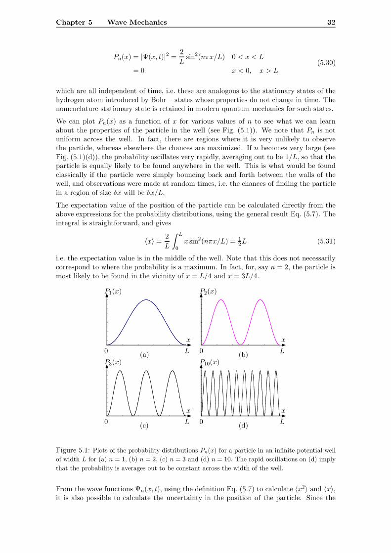
Chapter 5 Wave Mechanics 32
Pn(x) = |Ψ(x, t)|2 =2L
sin2(nπx/L) 0 < x < L
= 0 x < 0, x > L(5.30)
which are all independent of time, i.e. these are analogous to the stationary states of thehydrogen atom introduced by Bohr – states whose properties do not change in time. Thenomenclature stationary state is retained in modern quantum mechanics for such states.
We can plot Pn(x) as a function of x for various values of n to see what we can learnabout the properties of the particle in the well (see Fig. (5.1)). We note that Pn is notuniform across the well. In fact, there are regions where it is very unlikely to observethe particle, whereas elsewhere the chances are maximized. If n becomes very large (seeFig. (5.1)(d)), the probability oscillates very rapidly, averaging out to be 1/L, so that theparticle is equally likely to be found anywhere in the well. This is what would be foundclassically if the particle were simply bouncing back and forth between the walls of thewell, and observations were made at random times, i.e. the chances of finding the particlein a region of size δx will be δx/L.
The expectation value of the position of the particle can be calculated directly from theabove expressions for the probability distributions, using the general result Eq. (5.7). Theintegral is straightforward, and gives
〈x〉 =2L
∫ L
0x sin2(nπx/L) = 1
2L (5.31)
i.e. the expectation value is in the middle of the well. Note that this does not necessarilycorrespond to where the probability is a maximum. In fact, for, say n = 2, the particle ismost likely to be found in the vicinity of x = L/4 and x = 3L/4.
(a) (b)
(c) (d)
P1(x) P2(x)
P3(x) P10(x)
x x
x x
0 L 0 L
0 L 0 L
Figure 5.1: Plots of the probability distributions Pn(x) for a particle in an infinite potential wellof width L for (a) n = 1, (b) n = 2, (c) n = 3 and (d) n = 10. The rapid oscillations on (d) implythat the probability is averages out to be constant across the width of the well.
From the wave functions Ψn(x, t), using the definition Eq. (5.7) to calculate 〈x2〉 and 〈x〉,it is also possible to calculate the uncertainty in the position of the particle. Since the
Chapter 5 Wave Mechanics 33
probability distributions Pn(x) is symmetric about x = L/2, it is to be expected that〈x〉 = L/2. This can be readily confirmed by calculating the integral
〈x〉 =∫ L
0Pn(x) dx =
2L
∫ L
)x sin2(nπx/L) dx= 1
2L. (5.32)
The other expectation value 〈x2〉 is given by
〈x2〉 =2L
∫ L
0x2 sin2(nπx/L) dx = L2 2n2π2 − 3
6n2π2. (5.33)
Consequently, the uncertainty in position is
(∆x)2 = L2n2π2 − 3n2π2
− L2
4= L2n
2π2 − 612n2π2
. (5.34)
Orthonormality
An important feature of the wave functions derived above follows from considering thefollowing integral:∫ +∞
−∞ψ∗m(x)ψn(x) dx =
2L
∫ L
0
sin(mπx/L) sin(nπx/L) dx= δmn (5.35)
where δmn is known as the Kronecker delta, and ha the property that
δmn = 1 m = n
= 0 m �= n(5.36)
Thus, if m = n, the integral is unity, as it should be as this is just the normalization condi-tion that was imposed earlier on the wave functions. However, if m �= n, then the integralvanishes. The two wave functions are then said to be orthogonal, a condition somewhatanalogous to two vectors being orthogonal. The functions ψn for all n = 1, 2, 3, . . . arethen said to be orthonormal.
The property of orthonormality of eigenfunctions is found to be a general property of thestates of quantum systems that will be further explored in later Chapters.
Linear Superpositions
We found earlier that if we combine together wave functions of different wavelength andfrequency, corresponding to different particle momenta and energies, we produce somethingthat had an acceptable physical meaning – a wave packet. What we will do now is combinetogether – but in this case only two – different wave functions and see what meaning canbe given to the result obtained. Thus, we will consider the following linear combination,or linear superposition, of two wave functions:
Ψ(x, t) =1√2
[Ψ1(x, t) + Ψ2(x, t)
]=
1√L
[sin(πx/L)e−iω1t + sin(2πx/L)e−iω2t
]0 < x < L
= 0 x < 0 and x > L. (5.37)
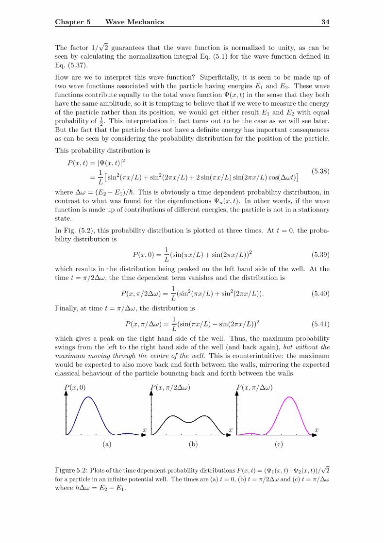
Chapter 5 Wave Mechanics 34
The factor 1/√
2 guarantees that the wave function is normalized to unity, as can beseen by calculating the normalization integral Eq. (5.1) for the wave function defined inEq. (5.37).
How are we to interpret this wave function? Superficially, it is seen to be made up oftwo wave functions associated with the particle having energies E1 and E2. These wavefunctions contribute equally to the total wave function Ψ(x, t) in the sense that they bothhave the same amplitude, so it is tempting to believe that if we were to measure the energyof the particle rather than its position, we would get either result E1 and E2 with equalprobability of 1
2 . This interpretation in fact turns out to be the case as we will see later.But the fact that the particle does not have a definite energy has important consequencesas can be seen by considering the probability distribution for the position of the particle.
This probability distribution is
P (x, t) = |Ψ(x, t)|2
=1L
[sin2(πx/L) + sin2(2πx/L) + 2 sin(πx/L) sin(2πx/L) cos(∆ωt)
] (5.38)
where ∆ω = (E2−E1)/�. This is obviously a time dependent probability distribution, incontrast to what was found for the eigenfunctions Ψn(x, t). In other words, if the wavefunction is made up of contributions of different energies, the particle is not in a stationarystate.
In Fig. (5.2), this probability distribution is plotted at three times. At t = 0, the proba-bility distribution is
P (x, 0) =1L
(sin(πx/L) + sin(2πx/L))2 (5.39)
which results in the distribution being peaked on the left hand side of the well. At thetime t = π/2∆ω, the time dependent term vanishes and the distribution is
P (x, π/2∆ω) =1L
(sin2(πx/L) + sin2(2πx/L)). (5.40)
Finally, at time t = π/∆ω, the distribution is
P (x, π/∆ω) =1L
(sin(πx/L)− sin(2πx/L))2 (5.41)
which gives a peak on the right hand side of the well. Thus, the maximum probabilityswings from the left to the right hand side of the well (and back again), but without themaximum moving through the centre of the well. This is counterintuitive: the maximumwould be expected to also move back and forth between the walls, mirroring the expectedclassical behaviour of the particle bouncing back and forth between the walls.
(a) (b) (c)
P (x, 0) P (x, π/2∆ω) P (x, π/∆ω)
x x x
Figure 5.2: Plots of the time dependent probability distributions P (x, t) = (Ψ1(x, t)+Ψ2(x, t))/√
2for a particle in an infinite potential well. The times are (a) t = 0, (b) t = π/2∆ω and (c) t = π/∆ωwhere �∆ω = E2 − E1.
Chapter 5 Wave Mechanics 35
As a final illustration, we can find the total probability of finding the particle on the lefthand half of the well, i.e. in the region 0 < x < L/2:
PL =∫ L/2
0P (x, t) dx = 1
2 + π−1 cos(∆ωt) (5.42)
while the corresponding result for the right hand side is
PR = 12 − π
−1 cos(∆ωt) (5.43)
which perhaps better illustrates the ‘see-sawing’ of the probability from one side to theother with a frequency of 2π∆ω.
What can be learned from this example is that if the wave function is made up of twocontributions of different energy, then the properties of the system do not stay constantin time, i.e. the system is no longer in a stationary state. Once again, the example of aparticle in a well illustrates a generic feature of quantum systems, namely that if they donot have a definite energy, then the properties of the system change in time.
Probability Distribution for Momentum
A final point to be considered here is that of determining what the momentum is of theparticle in the well. We cannot do this in an entirely correct fashion at this stage, butfor the purposes of further illustrating that the wave function contains more than justinformation on the position of the particle, we will use a slightly less rigorous argumentto arrive at essentially correct conclusions.
If we return to the eigenfunctions Ψn(x, t), we see that they can be written in the form
Ψn(x, t) =
√2L
ei(knx−ωnt) − e−i(knx+ωnt)
2i(5.44)
i.e. a linear combination of two counterpropagating waves, one associated with the particlehaving momentum pn = �kn, the other with the particle having momentum pn = −�kn.These two contributions enter the above expression with equal weight, by which is meantthat the magnitude of the coefficients of each of the exponentials is the same. It thereforeseems reasonable to suspect that the particle has an equal chance of being observed to havemomenta pn = ±�kn when the wave function of the particle is Ψn(x, t). This conjectureis consistent with what we would suppose is going on classically – the particle would bebouncing back and forth between the walls, simply reversing the direction of its momentumon each bounce. It should be pointed out that this is the argument alluded to above whichis not entirely correct. The momentum actually has a probability distribution which ispeaked at the values we have obtained here. The point can still be taken that informationon other than the position of the particle is to be found in the wave function.
Accepting this, we can then say that the particle has a chance of 12 of being observed to
have momentum �kn and a chance of 12 of being observed to have momentum −�kn, at
least if the wave function is Ψn(x, t). On this basis, we can calculate the expectation valueof the momentum, that is
〈p〉 = 12�kn + 1
2 (−�kn) = 0 (5.45)
and the expectation value of the momentum squared:
〈p2〉 = 12 (�kn)2 + 1
2 (−�kn)2 = �2k2n. (5.46)
Chapter 5 Wave Mechanics 36
Both these results are, in fact, exact.
The uncertainty in the momentum, ∆p, follows from
(∆p)2 = 〈p2〉 − 〈p〉2 = �2k2n = �
2(nπ/L)2. (5.47)
We can combine this with the result Eq. (5.34) for the uncertainty in the position to give
(∆x)2(∆p)2 = L2n2π2 − 612n2π2
�2(nπ/L)2 =
�2
4
(n2π2 − 63
). (5.48)
Since the term (n2π2 − 6)/3) is always bigger than unity (at the smallest, when n = 1, itis 1.29), we have
(∆x)2(∆p)2 ≥ �2
4(5.49)
or, in other words
∆x∆p ≥ 12� (5.50)
in agreement with the Heisenberg uncertainty principle, Eq. (3.14).
5.4 The Schrodinger Wave Equation
So far, we have made a lot of progress concerning the properties of, and interpretation ofthe wave function, but as yet we have had very little to say about how the wave functionmay be derived in a general situation, that is to say, we do not have on hand a ‘waveequation’ for the wave function. There is no true derivation of this equation, but its formcan be motivated by physical and mathematical arguments at a wide variety of levels ofsophistication. Here, we will offer a simple derivation based on what we have learned sofar about the wave function.
In the discussion of the particle in an infinite potential well, it was observed that thewave function of a particle of fixed energy E could most naturally be written as a linearcombination of wave functions of the form
Ψ(x, t) = Aei(kx−ωt) (5.51)
representing a wave travelling in the positive x direction, and a corresponding wave trav-elling in the opposite direction, so giving rise to a standing wave, this being necessaryin order to satisfy the boundary conditions. This corresponds intuitively to our classicalnotion of a particle bouncing back and forth between the walls of the potential well, whichsuggests that we adopt the wave function above as being the appropriate wave functionfor a free particle of momentum p = �k and energy E = �ω. With this in mind, we canthen note that
∂2Ψ∂x2
= −k2Ψ (5.52)
which can be written, using E = p2/2m = �2k2/2m:
− �2
2m∂2Ψ∂x2
=p2
2mΨ. (5.53)
Chapter 5 Wave Mechanics 37
Similarly
∂Ψ∂t
= −iωΨ (5.54)
which can be written, using E = �ω:
i�∂Ψ∂t
= �ωψ = EΨ. (5.55)
We now generalize this to the situation in which there is both a kinetic energy and apotential energy present, then E = p2/2m+ V (x) so that
EΨ =p2
2mΨ + V (x)Ψ (5.56)
where Ψ is now the wave function of a particle moving in the presence of a potential V (x).But if we assume that the results Eq. (5.53) and Eq. (5.55) still apply in this case then wehave
− �2
2m∂2ψ
∂x2+ V (x)Ψ = i�
∂ψ
∂t(5.57)
which is the famous Schrodinger wave equation. We will not be much concerned withsolving this equation here, but it is worthwhile to point out that it is the basic equationof that branch of quantum mechanics known as wave mechanics.
5.5 Is the Wave Function all that is Needed?
So far, we have been concerned almost entirely with the quantum mechanics associatedwith the motion of particles through space, which may give rise to the mistaken notion thatall of quantum mechanics revolves around the idea of the wave function. However, this isfar from the case. There is no objective reality that can be attached to the wave function –it is just one of many ways that the quantum nature of matter can be expressed. It is usefulfor many kinds of problems, but entirely inappropriate for others, and a singular focus onthe wave function can give the impression that the wave function is the heart of quantummechanics. But the quantum mechanical nature of matter makes itself known in waysthat have little to do with waves and wave functions. Correspondingly, the mathematicaltheory of quantum mechanics is much more than just the mathematics of waves.
But what are the other aspects of quantum mechanics that need more than wave mechan-ics? For one thing, it can be shown there is no such thing as a wave function for a photon.There are many physical processes in which the physically observable quantity is not wherea particle is, or how fast it is moving, but rather how many particles there are of a certainkind – an important consideration as particles can be created or destroyed in a randomway. The whole subject of the quantum theory of fields is expressed in the language ofparticle numbers. But one of the most important examples of a circumstance in whichwave mechanics falls short is in describing the intrinsic spin of elementary particles. Inthe following Chapter, attention will be focussed on the example of particle spin and theStern-Gerlach experiment as being a way of illustrating some of the general principles ofquantum mechanics.
Chapter 6
Particle Spin and theStern-Gerlach Experiment
The spin of an elementary particle would appear, on the surface, to be little different fromthe spin of a macroscopic object – the image of a microscopic sphere spinning aroundsome axis comes to mind. However, there is far more going on here than what this simplepicture might suggest. But first, a brief look at what the classical properties are of angularmomentum is needed.
6.1 Classical Spin Angular Momentum
A particle moving through space possesses angular momentum, a vector, defined by
L = r× p (6.1)
where r and p are the position vector and momentum respectively of the particle. This issometimes referred to as orbital angular momentum since, in particular, it is an importantconsideration in describing the properties of a particle orbiting around some centre ofattraction such as, in the classical picture of an atom, electrons orbiting around an atomicnucleus. Classically there is no restriction on the magnitude or direction of orbital angularmomentum.
From a classical perspective, as an electron carries a charge, its orbital motion will resultin a tiny current loop which will produce a dipolar magnetic field. The strength of thisdipole field is measured by the magnetic moment µµµ which is related to the orbital angularmomentum by
µLµLµL =q
2mL. (6.2)
Thus, the expectation on the basis of this classical picture is that atoms can behave astiny little magnets.
The classical idea of spin follows directly from the above considerations. Spin is the angularmomentum we associate with a rotating object such as a spinning golf ball, or the spinningEarth. The angular momentum of such a body can be calculated by integrating over thecontributions to the angular momentum due to the motion of each of the infinitesimal
Chapter 6 Particle Spin and the Stern-Gerlach Experiment 39
masses making up the body. The well known result is that the total angular momentumor spin S is given by
S = Iωωω (6.3)
where I is the moment of inertia of the body, and ωωω is its angular velocity. Spin is a vectorwhich points along the axis of rotation in a direction determined by the right hand rule:curl the fingers of the right hand in the direction of rotation and the thumb points in thedirection of S. The moment of inertia is determined by the distribution of mass in therotating body relative to the axis of rotation. If the object were a solid uniform sphere ofmass m and radius a, and rotation were about a diameter of the sphere, then the momentof inertia can be shown to be
I = 25Ma2. (6.4)
If the sphere possesses an electric charge, then the circulation of the charge around the axisof rotation will constitute a current and hence will give rise to a magnetic field. This fieldis a dipole field whose strength is measured by the dipole moment which can be shown,for a uniformly charged sphere of total charge q, to be given by
µSµSµS =q
2mS, (6.5)
exactly the same as in the orbital case.
The point to be made here is that the spinning object is extended in space, i.e. the spinningsphere example has a non-zero radius. If we try to extend the idea to a point particle bytaking the limit of a → 0 we immediately see that the spin angular momentum mustvanish unless ω is allowed to be infinitely large. If we exclude this last possibility, thenclassically a point particle cannot have spin angular momentum or, for that matter, amagnetic moment. From the point-of-view of classical physics, elementary particles suchas an electron, which are known to possess spin angular momentum, cannot be viewed aspoint objects – they must be considered as tiny spinning spheres. But as far as it has beenpossible to determine by high energy scattering experiments, elementary particles such asthe electron behave very much as point particles. Whatever radius they might have, it iscertainly very tiny: experiment suggests it is less than < 10−17 m. Yet they are found topossess spin angular momentum of a magnitude equal (for the electron) to
√3/�/2 which
requires the surface of the particle to be moving at a speed greater than that of light.This conflict with special relativity makes this classical picture of an elementary particleas a tiny, rapidly rotating sphere obviously untenable. Quantum mechanics offers someresolution to the problem, though,as we shall see, it is not in terms of the wave function.
6.2 Quantum Spin Angular Momentum
Wave mechanics and the wave function describe the properties of a particle moving throughspace, giving, as we have seen, information on its position, momentum, energy. In additionit also provides a quantum description of the orbital angular momentum of a particle, suchas that associated with an electron moving in an orbit around an atomic nucleus. Thegeneral results found are that the magnitude of the angular momentum is limited to thevalues
L =√l(l+ 1)�, l = 0, 1, 2, 3, . . . , (6.6)
Chapter 6 Particle Spin and the Stern-Gerlach Experiment 40
which can be looked on as an ‘improved’ version of the result used by Bohr and ‘justified’by the de Broglie hypothesis, that is L = n�, Eq. (2.1). The theory also tells us that anyone vector component of L, Lz say, is restricted to the values
Lz = ml�, ml = −l,−l+ 1,−l+ 2, . . . l − 2, l− 1, l. (6.7)
This restriction on the possible values of Lz mean that the angular momentum vector canhave only certain orientations in space – a result known as ‘space quantization’.
All this is built around the quantum mechanical version of L = r×p, and so implicitly isconcerned with the angular momentum of a particle moving through space. But a moregeneral perspective yields some surprises. If special relativity and quantum mechanics arecombined, it is found that even if a particle, a point object, has zero momentum, so thatthe orbital angular momentum is zero, its total angular momentum is, in general, not zero.The only interpretation that can be offered is that this angular momentum is due to theintrinsic spin of the particle. The possible values for the magnitude S of the spin angularmomentum turn out to be
S =√s(s + 1)�, s = 0, 1
2 , 1,32 , 2 . . . , (6.8)
and any one vector component of S, Sz say, is restricted to the values
Sz = ml�, ms = −s,−s+ 1,−s+ 2, . . . s− 2, s− 1, s (6.9)
i.e. the same as for orbital angular momentum, but with the significant difference ofthe appearance of half integer values for the spin quantum number s in addition to theinteger values. This theoretical result is confirmed by experiment. In nature there existelementary particles for which s = 1
2 ,32 ,
52 . . . such as the electron, proton, neutron, quark
(all of which have spin s = 12 ), and more exotic particles of higher half-integer spin, while
there exist many particles with integer spin, the photon, for which s = 1, being the mostwell-known example.
While wave mechanics can yield the integer values for the spin angular momentum quan-tum number, this is in some sense a fortuitous result. The fact is that particle spin is whatis left after the contribution to the angular momentum due to motion through space hasbeen removed. It is angular momentum associated with the internal degrees of freedom ofa point particle, whatever they may be, and cannot be described mathematically in termsof a wave function. It also has no classical analogue: we have already seen that a pointparticle cannot have spin angular momentum. Thus, particle spin is a truly quantumproperty that cannot be described in the language of wave functions – a more generalmathematical language is required. It was in fact the discovery of particle spin, in par-ticular the spin of the electron, that lead to the development of a more general version ofquantum mechanics than that implied by wave mechanics.
There is one classical property of angular momentum that carries over to quantum mechan-ics. If the particle is charged, and if it possesses either orbital or spin angular momentum,then there arises a dipole magnetic field. In the case of the electron, the dipole momentis found to be given by
µSµSµS = − e
2megS (6.10)
where me and −e are the mass and charge of the electron, S is the spin angular momentumof the electron, and g is the so-called gyromagnetic ratio, which classically is exactly equalto one, but is known (both from measurement and as derived from relativistic quantummechanics) to be approximately equal to two for an electron. It is the fact that electronspossess a magnetic moment that has made it possible to perform experiments involvingthe spin of electrons, in a way that reveals the intrinsically quantum properties of spin.
Chapter 6 Particle Spin and the Stern-Gerlach Experiment 41
6.3 The Stern-Gerlach Experiment
This experiment, first performed in 1922, has long been considered as the quintessentialexperiment that illustrates the fact that the electron possesses intrinsic angular momen-tum, i.e. spin. It is actually the case that the original experiment nothing to do with thediscovery that the electron possessed spin: the first proposal concerning the spin of theelectron, made in 1925 by Uhlenbech and Goudsmit, was based on the analysis of atomicspectra. What the experiment was intended to test was ‘space-quantization’ associatedwith the orbital angular momentum of atomic electrons. The prediction, already made bythe ‘old’ quantum theory that developed out of Bohr’s work, was that the spatial compo-nents of angular momentum could only take discrete values, so that the direction of theangular momentum vector was restricted to only a limited number of possibilities, andthis could be tested by making use of the fact that an orbiting electron will give rise to amagnetic moment proportional to the orbital angular momentum of the electron. So, bymeasuring the magnetic moment of an atom, it should be possible to determine whetheror not space quantization existed. In fact, the results of the experiment were in agreementwith the then existing (incorrect) quantum theory – the existence of electron spin was notat that time suspected. Later, it was realized that the interpretation of the results of theexperiment were incorrect, and that what was seen in the experiment was direct evidencethat an electrons possess spin. It is in this way that the Stern-Gerlach experiment hassubsequently been used, i.e. to illustrate the fact that electrons have spin. But it is alsovaluable in another way. The simplicity of the results of the experiment (only two possibleoutcomes), and the fact that the experiment produces results that are directly evidence ofthe laws of quantum mechanics in action makes it an ideal means by which the essentialfeatures of quantum mechanics can be seen and, perhaps, ‘understood’.
The original experimental arrangement took the form of a collimated beam of silver atomsheading in, say, the y direction, and passing through a non-uniform magnetic field di-rected (mostly) in the z-direction. Assuming the silver atoms possess a non-zero magneticmoment µµµ, the magnetic field will have two effects. First, the magnetic field will exerta torque on the magnetic dipole, so that the magnetic moment vector will precess aboutthe direction of the magnetic field. This will not affect the z component of µµµ, but the xand y components of µµµ will change with time. Secondly, and more importantly here, thenon-uniformity of the field means that the atoms experience a sideways force given by
Fz = −∂U∂z
(6.11)
where U = −µµµ ·B = µzB is the potential energy of the silver atom in the magnetic field.Thus
Fz = −µz∂B
∂z. (6.12)
Different orientations of the magnetic moment vector µµµ will lead to different values of µz,which in turn will mean that there will be forces acting on the atoms which will differdepending on the value of µz .
The expectation based on classical physics is that due to random thermal effects in theoven, the magnetic dipole moment vectors of the atoms will be randomly oriented in space,so there should be a continuous spread in the z component of the magnetic moments ofthe silver atoms as they emerge from the oven, ranging from −|µz| to |µz|. A line shouldthen appear on the observation screen along the z direction. Instead, what was found
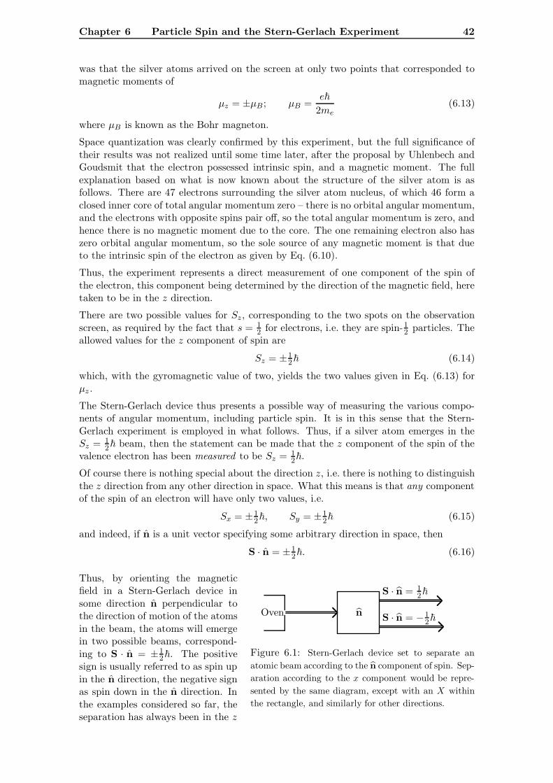
Chapter 6 Particle Spin and the Stern-Gerlach Experiment 42
was that the silver atoms arrived on the screen at only two points that corresponded tomagnetic moments of
µz = ±µB ; µB =e�
2me(6.13)
where µB is known as the Bohr magneton.
Space quantization was clearly confirmed by this experiment, but the full significance oftheir results was not realized until some time later, after the proposal by Uhlenbech andGoudsmit that the electron possessed intrinsic spin, and a magnetic moment. The fullexplanation based on what is now known about the structure of the silver atom is asfollows. There are 47 electrons surrounding the silver atom nucleus, of which 46 form aclosed inner core of total angular momentum zero – there is no orbital angular momentum,and the electrons with opposite spins pair off, so the total angular momentum is zero, andhence there is no magnetic moment due to the core. The one remaining electron also haszero orbital angular momentum, so the sole source of any magnetic moment is that dueto the intrinsic spin of the electron as given by Eq. (6.10).
Thus, the experiment represents a direct measurement of one component of the spin ofthe electron, this component being determined by the direction of the magnetic field, heretaken to be in the z direction.
There are two possible values for Sz, corresponding to the two spots on the observationscreen, as required by the fact that s = 1
2 for electrons, i.e. they are spin-12 particles. The
allowed values for the z component of spin are
Sz = ±12� (6.14)
which, with the gyromagnetic value of two, yields the two values given in Eq. (6.13) forµz .
The Stern-Gerlach device thus presents a possible way of measuring the various compo-nents of angular momentum, including particle spin. It is in this sense that the Stern-Gerlach experiment is employed in what follows. Thus, if a silver atom emerges in theSz = 1
2� beam, then the statement can be made that the z component of the spin of thevalence electron has been measured to be Sz = 1
2�.
Of course there is nothing special about the direction z, i.e. there is nothing to distinguishthe z direction from any other direction in space. What this means is that any componentof the spin of an electron will have only two values, i.e.
Sx = ±12�, Sy = ±1
2� (6.15)
and indeed, if n is a unit vector specifying some arbitrary direction in space, then
S · n = ±12�. (6.16)
Thus, by orienting the magneticfield in a Stern-Gerlach device insome direction n perpendicular tothe direction of motion of the atomsin the beam, the atoms will emergein two possible beams, correspond-ing to S · n = ±1
2�. The positivesign is usually referred to as spin upin the n direction, the negative signas spin down in the n direction. Inthe examples considered so far, theseparation has always been in the z
Oven n
S · n = 12�
S · n = −12�
Figure 6.1: Stern-Gerlach device set to separate anatomic beam according to the n component of spin. Sep-aration according to the x component would be repre-sented by the same diagram, except with an X withinthe rectangle, and similarly for other directions.
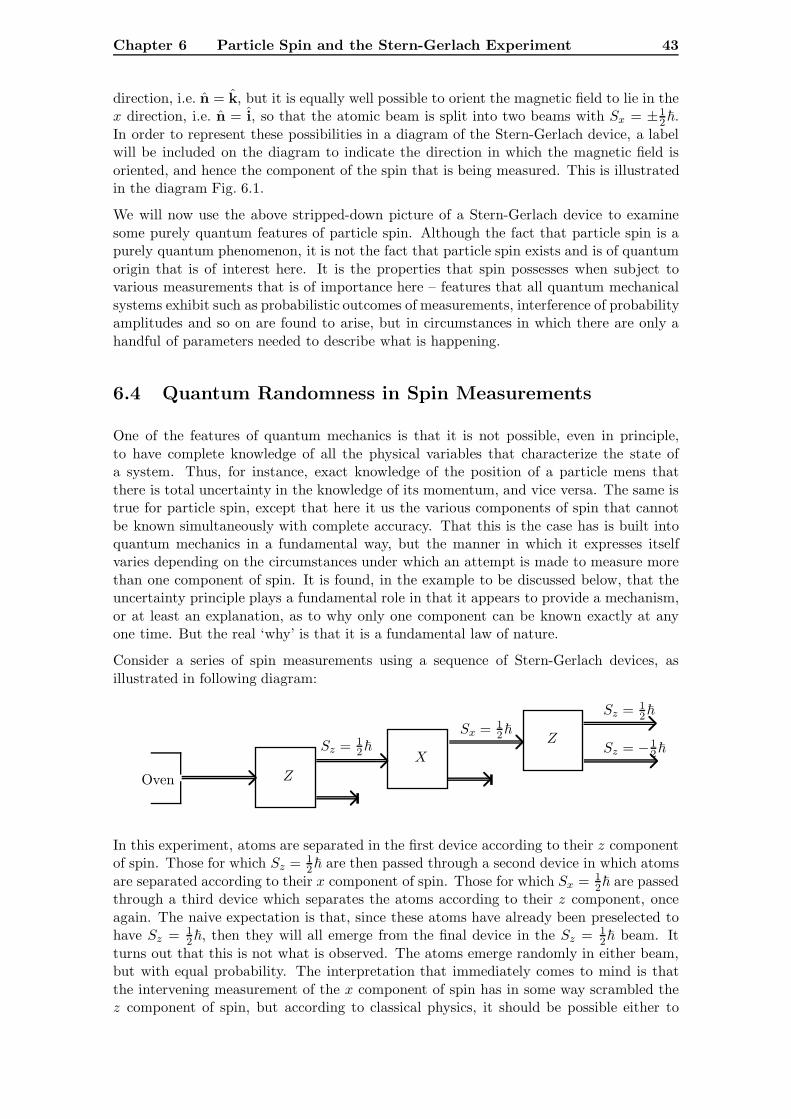
Chapter 6 Particle Spin and the Stern-Gerlach Experiment 43
direction, i.e. n = k, but it is equally well possible to orient the magnetic field to lie in thex direction, i.e. n = i, so that the atomic beam is split into two beams with Sx = ±1
2�.In order to represent these possibilities in a diagram of the Stern-Gerlach device, a labelwill be included on the diagram to indicate the direction in which the magnetic field isoriented, and hence the component of the spin that is being measured. This is illustratedin the diagram Fig. 6.1.
We will now use the above stripped-down picture of a Stern-Gerlach device to examinesome purely quantum features of particle spin. Although the fact that particle spin is apurely quantum phenomenon, it is not the fact that particle spin exists and is of quantumorigin that is of interest here. It is the properties that spin possesses when subject tovarious measurements that is of importance here – features that all quantum mechanicalsystems exhibit such as probabilistic outcomes of measurements, interference of probabilityamplitudes and so on are found to arise, but in circumstances in which there are only ahandful of parameters needed to describe what is happening.
6.4 Quantum Randomness in Spin Measurements
One of the features of quantum mechanics is that it is not possible, even in principle,to have complete knowledge of all the physical variables that characterize the state ofa system. Thus, for instance, exact knowledge of the position of a particle mens thatthere is total uncertainty in the knowledge of its momentum, and vice versa. The same istrue for particle spin, except that here it us the various components of spin that cannotbe known simultaneously with complete accuracy. That this is the case has is built intoquantum mechanics in a fundamental way, but the manner in which it expresses itselfvaries depending on the circumstances under which an attempt is made to measure morethan one component of spin. It is found, in the example to be discussed below, that theuncertainty principle plays a fundamental role in that it appears to provide a mechanism,or at least an explanation, as to why only one component can be known exactly at anyone time. But the real ‘why’ is that it is a fundamental law of nature.
Consider a series of spin measurements using a sequence of Stern-Gerlach devices, asillustrated in following diagram:
Z
X
Z
Oven
Sz = 12�
Sx = 12�
Sz = 12�
Sz = −12�
In this experiment, atoms are separated in the first device according to their z componentof spin. Those for which Sz = 1
2� are then passed through a second device in which atomsare separated according to their x component of spin. Those for which Sx = 1
2� are passedthrough a third device which separates the atoms according to their z component, onceagain. The naive expectation is that, since these atoms have already been preselected tohave Sz = 1
2�, then they will all emerge from the final device in the Sz = 12� beam. It
turns out that this is not what is observed. The atoms emerge randomly in either beam,but with equal probability. The interpretation that immediately comes to mind is thatthe intervening measurement of the x component of spin has in some way scrambled thez component of spin, but according to classical physics, it should be possible either to
Chapter 6 Particle Spin and the Stern-Gerlach Experiment 44
arrange the experiment such that any such scrambling be made negligibly small, or else beable to correct for the apparent scrambling in some fashion. It turns out that the quantumeffects prevent this from happening – this scrambling, and the consequent introduction ofrandomness into the outcome of the experiment cannot be avoided, except at the cast ofnot being able to measure the x component of spin at all! Thus we see again an exampleof intrinsic randomness in the behaviour of macroscopic systems.
In the following section, an argument is presented which shows how it is that quantumeffects prevent the simultaneous exact measurement of both the x and the z componentsof spin i.e. that it is uncontrollable quantum effects that give rise to the scrambling of thez component of spin during the measurement of the x component.
6.4.1 Incompatible Measurements of Spin Components
The obvious question to ask is whether or not the experiment can be refined in some wayto avoid this scrambling. From the perspective of classical physics, the answer is definitelyyes, at least in principle. The problem is that the atoms, as they pass through the secondStern-Gerlach device, will experience precession about the x axis which will have theeffect of changing the z component of the spin. But by suitable fiddling with the beam,the magnetic field strengths and so on it should be possible in principle, at least from thepoint of view of classical physics, to minimize this effect, or at least determine exactlyhow much precession occurs, and take account of it. But in practice, it turns out that allthese attempts fail. If the experiment is refined in such a manner that the precession ismade negligible, (e.g. by using faster atoms, or a weaker magnetic field), the result is thatthe two emerging beams overlap so much that it is impossible to tell which beam an atombelongs to, i.e. we retain exact information on the z component of spin, but learn nothingabout the x component! In general, it appears that it is not possible to measure both Szand Sx (or, indeed any pair of components of the particle spin), precisely. This kind ofbehaviour is reminiscent of what is found to happen when we attempt to measure boththe position and the momentum of a particle. According to the uncertainty principle,the more precisely we determine the position of a particle, the less we know about themomentum of the particle. The difference here is that the quantities being measured arediscrete – they have only two possible values, whereas the position and momentum of afree particle (even in quantum mechanics) can assume a continuous range of values.
A Detailed Analysis By use of a hybrid mixture of classical and quantum mechanicalarguments, it is possible to come to some ‘understanding’ of why this occurs. Considerthe atoms that have left the first Stern-Gerlach device with Sz = 1
2� and enter the nextdevice which has a magnetic field B = Bi oriented in the x direction. This magnetic fieldis non-uniform, in other words B is a function of position – it could be written B(x, y, z).The experimental arrangement is such that the non-uniformity is most marked in the xdirection – it is this non-uniformity that is responsible for the forces acting to deflect theatoms as they move through the device. In fact, the interaction of the magnetic momentµµµ of the atoms with this non-uniform magnetic field has two consequences. First, as justmentioned, the atoms feel a force in the x direction given by
Fx = −µx∂B
∂x(6.17)
where µx is the x component of the magnetic moment of the atoms. If we accept in thisotherwise classical argument that the values of the spin of an electron are restricted to
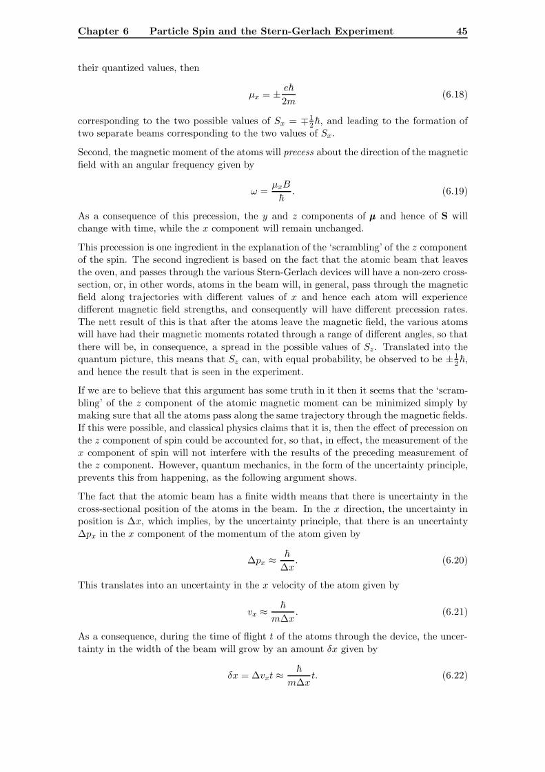
Chapter 6 Particle Spin and the Stern-Gerlach Experiment 45
their quantized values, then
µx = ± e�
2m(6.18)
corresponding to the two possible values of Sx = ∓12�, and leading to the formation of
two separate beams corresponding to the two values of Sx.
Second, the magnetic moment of the atoms will precess about the direction of the magneticfield with an angular frequency given by
ω =µxB
�. (6.19)
As a consequence of this precession, the y and z components of µµµ and hence of S willchange with time, while the x component will remain unchanged.
This precession is one ingredient in the explanation of the ‘scrambling’ of the z componentof the spin. The second ingredient is based on the fact that the atomic beam that leavesthe oven, and passes through the various Stern-Gerlach devices will have a non-zero cross-section, or, in other words, atoms in the beam will, in general, pass through the magneticfield along trajectories with different values of x and hence each atom will experiencedifferent magnetic field strengths, and consequently will have different precession rates.The nett result of this is that after the atoms leave the magnetic field, the various atomswill have had their magnetic moments rotated through a range of different angles, so thatthere will be, in consequence, a spread in the possible values of Sz. Translated into thequantum picture, this means that Sz can, with equal probability, be observed to be ±1
2�,and hence the result that is seen in the experiment.
If we are to believe that this argument has some truth in it then it seems that the ‘scram-bling’ of the z component of the atomic magnetic moment can be minimized simply bymaking sure that all the atoms pass along the same trajectory through the magnetic fields.If this were possible, and classical physics claims that it is, then the effect of precession onthe z component of spin could be accounted for, so that, in effect, the measurement of thex component of spin will not interfere with the results of the preceding measurement ofthe z component. However, quantum mechanics, in the form of the uncertainty principle,prevents this from happening, as the following argument shows.
The fact that the atomic beam has a finite width means that there is uncertainty in thecross-sectional position of the atoms in the beam. In the x direction, the uncertainty inposition is ∆x, which implies, by the uncertainty principle, that there is an uncertainty∆px in the x component of the momentum of the atom given by
∆px ≈�
∆x. (6.20)
This translates into an uncertainty in the x velocity of the atom given by
vx ≈�
m∆x. (6.21)
As a consequence, during the time of flight t of the atoms through the device, the uncer-tainty in the width of the beam will grow by an amount δx given by
δx = ∆vxt ≈�
m∆xt. (6.22)
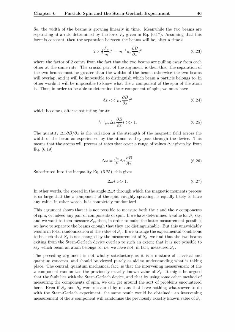
Chapter 6 Particle Spin and the Stern-Gerlach Experiment 46
So, the width of the beams is growing linearly in time. Meanwhile the two beams areseparating at a rate determined by the force Fx given in Eq. (6.17). Assuming that thisforce is constant, then the separation between the beams will be, after a time t
2× 12
Fxmt2 = m−1µx
∂B
∂xt2 (6.23)
where the factor of 2 comes from the fact that the two beams are pulling away from eachother at the same rate. The crucial part of the argument is then this: the separation ofthe two beams must be greater than the widths of the beams otherwise the two beamswill overlap, and it will be impossible to distinguish which beam a particle belongs to, inother words it will be impossible to know what the x component of the spin of the atomis. Thus, in order to be able to determine the x component of spin, we must have
δx << µx∂B
∂xt2 (6.24)
which becomes, after substituting for δx
�−1µx∆x
∂B
∂xt >> 1. (6.25)
The quantity ∆x∂B/∂x is the variation in the strength of the magnetic field across thewidth of the beam as experienced by the atoms as they pass through the device. Thismeans that the atoms will precess at rates that cover a range of values ∆ω given by, fromEq. (6.19)
∆ω =µx�
∆x∂B
∂x. (6.26)
Substituted into the inequality Eq. (6.25), this gives
∆ωt >> 1. (6.27)
In other words, the spread in the angle ∆ωt through which the magnetic moments precessis so large that the z component of the spin, roughly speaking, is equally likely to haveany value, in other words, it is completely randomized.
This argument shows that it is not possible to measure both the z and the x componentsof spin, or indeed any pair of components of spin. If we have determined a value for Sz say,and we want to then measure Sx, then, in order to make the latter measurement possible,we have to separate the beams enough that they are distinguishable. But this unavoidablyresults in total randomization of the value of Sz. If we arrange the experimental conditionsto be such that Sz is not changed by the measurement of Sx, we find that the two beamsexiting from the Stern-Gerlach device overlap to such an extent that it is not possible tosay which beam an atom belongs to, i.e. we have not, in fact, measured Sx.
The preceding argument is not wholly satisfactory as it is a mixture of classical andquantum concepts, and should be viewed purely as aid to understanding what is takingplace. The central, quantum mechanical fact, is that the intervening measurement of thex component randomizes the previously exactly known value of Sz. It might be arguedthat the fault lies with the Stern-Gerlach device, and that by using some other method ofmeasuring the components of spin, we can get around the sort of problems encounteredhere. Even if Sx and Sz were measured by means that have nothing whatsoever to dowith the Stern-Gerlach experiment, the same result would be obtained: an interveningmeasurement of the x component will randomize the previously exactly known value of Sz.
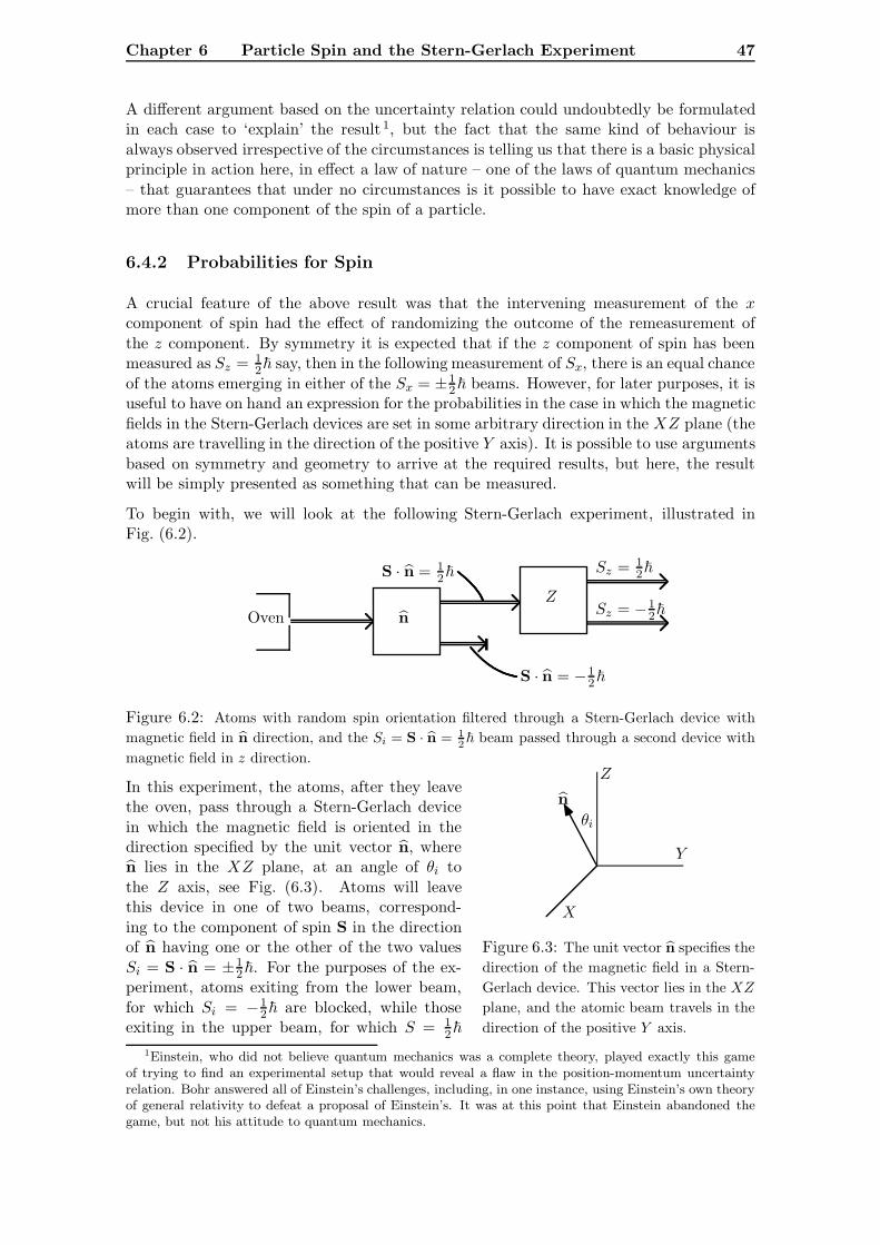
Chapter 6 Particle Spin and the Stern-Gerlach Experiment 47
A different argument based on the uncertainty relation could undoubtedly be formulatedin each case to ‘explain’ the result 1, but the fact that the same kind of behaviour isalways observed irrespective of the circumstances is telling us that there is a basic physicalprinciple in action here, in effect a law of nature – one of the laws of quantum mechanics– that guarantees that under no circumstances is it possible to have exact knowledge ofmore than one component of the spin of a particle.
6.4.2 Probabilities for Spin
A crucial feature of the above result was that the intervening measurement of the xcomponent of spin had the effect of randomizing the outcome of the remeasurement ofthe z component. By symmetry it is expected that if the z component of spin has beenmeasured as Sz = 1
2� say, then in the following measurement of Sx, there is an equal chanceof the atoms emerging in either of the Sx = ±1
2� beams. However, for later purposes, it isuseful to have on hand an expression for the probabilities in the case in which the magneticfields in the Stern-Gerlach devices are set in some arbitrary direction in the XZ plane (theatoms are travelling in the direction of the positive Y axis). It is possible to use argumentsbased on symmetry and geometry to arrive at the required results, but here, the resultwill be simply presented as something that can be measured.
To begin with, we will look at the following Stern-Gerlach experiment, illustrated inFig. (6.2).
nZ
Oven
S · n = 12�
S · n = −12�
Sz = 12�
Sz = −12�
Figure 6.2: Atoms with random spin orientation filtered through a Stern-Gerlach device withmagnetic field in n direction, and the Si = S · n = 1
2� beam passed through a second device with
magnetic field in z direction.
In this experiment, the atoms, after they leavethe oven, pass through a Stern-Gerlach devicein which the magnetic field is oriented in thedirection specified by the unit vector n, wheren lies in the XZ plane, at an angle of θi tothe Z axis, see Fig. (6.3). Atoms will leavethis device in one of two beams, correspond-ing to the component of spin S in the directionof n having one or the other of the two valuesSi = S · n = ±1
2�. For the purposes of the ex-periment, atoms exiting from the lower beam,for which Si = −1
2� are blocked, while thoseexiting in the upper beam, for which S = 1
2�
X
Y
Z
nθi
Figure 6.3: The unit vector n specifies thedirection of the magnetic field in a Stern-Gerlach device. This vector lies in the XZplane, and the atomic beam travels in thedirection of the positive Y axis.
1Einstein, who did not believe quantum mechanics was a complete theory, played exactly this gameof trying to find an experimental setup that would reveal a flaw in the position-momentum uncertaintyrelation. Bohr answered all of Einstein’s challenges, including, in one instance, using Einstein’s own theoryof general relativity to defeat a proposal of Einstein’s. It was at this point that Einstein abandoned thegame, but not his attitude to quantum mechanics.
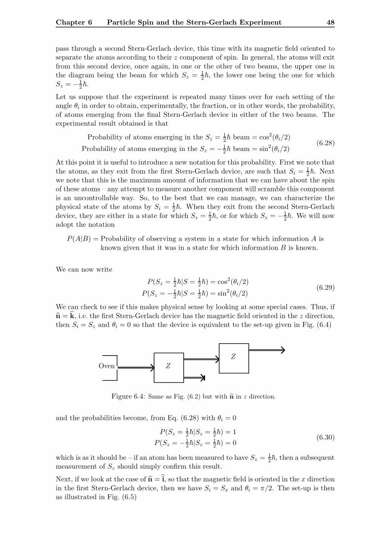
Chapter 6 Particle Spin and the Stern-Gerlach Experiment 48
pass through a second Stern-Gerlach device, this time with its magnetic field oriented toseparate the atoms according to their z component of spin. In general, the atoms will exitfrom this second device, once again, in one or the other of two beams, the upper one inthe diagram being the beam for which Sz = 1
2�, the lower one being the one for whichSz = −1
2�.
Let us suppose that the experiment is repeated many times over for each setting of theangle θi in order to obtain, experimentally, the fraction, or in other words, the probability,of atoms emerging from the final Stern-Gerlach device in either of the two beams. Theexperimental result obtained is that
Probability of atoms emerging in the Sz = 12� beam = cos2(θi/2)
Probability of atoms emerging in the Sz = −12� beam = sin2(θi/2)
(6.28)
At this point it is useful to introduce a new notation for this probability. First we note thatthe atoms, as they exit from the first Stern-Gerlach device, are such that Si = 1
2�. Nextwe note that this is the maximum amount of information that we can have about the spinof these atoms – any attempt to measure another component will scramble this componentis an uncontrollable way. So, to the best that we can manage, we can characterize thephysical state of the atoms by Si = 1
2�. When they exit from the second Stern-Gerlachdevice, they are either in a state for which Sz = 1
2�, or for which Sz = −12�. We will now
adopt the notation
P (A|B) = Probability of observing a system in a state for which information A isknown given that it was in a state for which information B is known.
We can now write
P (Sz = 12�|S = 1
2�) = cos2(θi/2)
P (Sz = −12�|S = 1
2�) = sin2(θi/2)(6.29)
We can check to see if this makes physical sense by looking at some special cases. Thus, ifn = k, i.e. the first Stern-Gerlach device has the magnetic field oriented in the z direction,then Si = Sz and θi = 0 so that the device is equivalent to the set-up given in Fig. (6.4)
Z
Z
Oven
Figure 6.4: Same as Fig. (6.2) but with n in z direction.
and the probabilities become, from Eq. (6.28) with θi = 0
P (Sz = 12�|Sz = 1
2�) = 1P (Sz = −1
2�|Sz = 12�) = 0
(6.30)
which is as it should be – if an atom has been measured to have Sz = 12�, then a subsequent
measurement of Sz should simply confirm this result.
Next, if we look at the case of n = i, so that the magnetic field is oriented in the x directionin the first Stern-Gerlach device, then we have Si = Sx and θi = π/2. The set-up is thenas illustrated in Fig. (6.5)
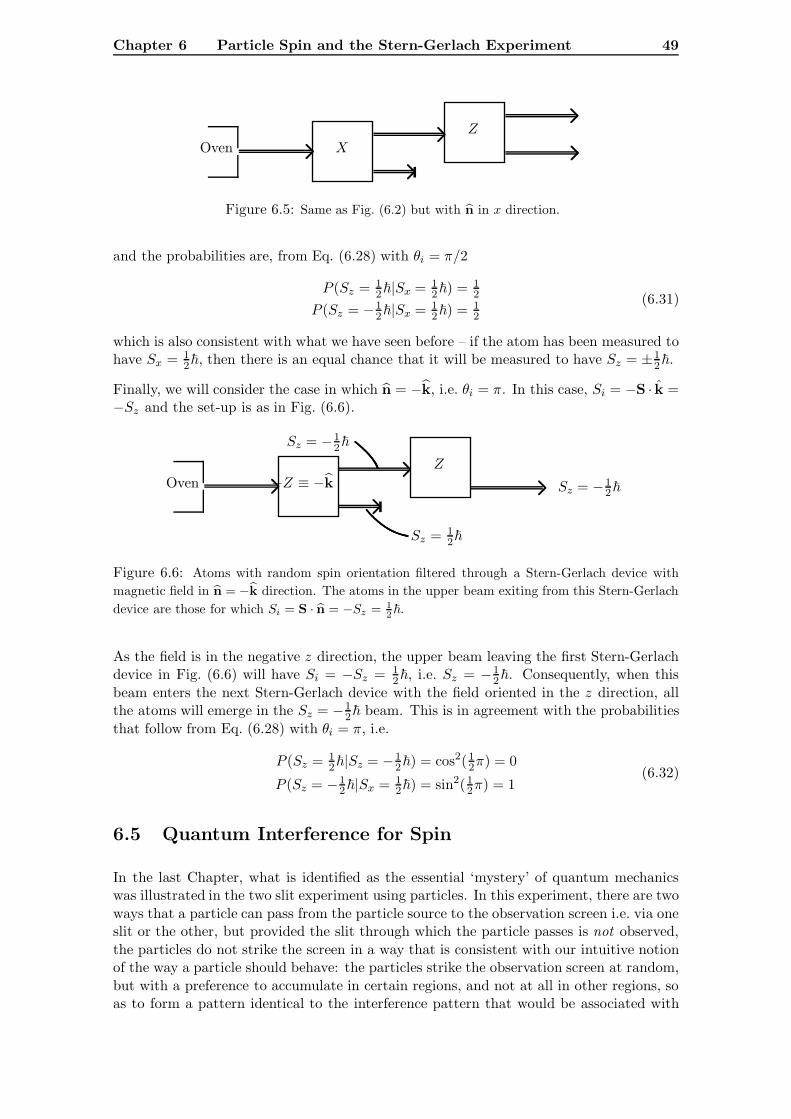
Chapter 6 Particle Spin and the Stern-Gerlach Experiment 49
X
Z
Oven
Figure 6.5: Same as Fig. (6.2) but with n in x direction.
and the probabilities are, from Eq. (6.28) with θi = π/2
P (Sz = 12�|Sx = 1
2�) = 12
P (Sz = −12�|Sx = 1
2�) = 12
(6.31)
which is also consistent with what we have seen before – if the atom has been measured tohave Sx = 1
2�, then there is an equal chance that it will be measured to have Sz = ±12�.
Finally, we will consider the case in which n = −k, i.e. θi = π. In this case, Si = −S · k =−Sz and the set-up is as in Fig. (6.6).
−Z ≡ −kZ
Oven
Sz = −12�
Sz = 12�
Sz = −12�
Figure 6.6: Atoms with random spin orientation filtered through a Stern-Gerlach device withmagnetic field in n = −k direction. The atoms in the upper beam exiting from this Stern-Gerlachdevice are those for which Si = S · n = −Sz = 1
2�.
As the field is in the negative z direction, the upper beam leaving the first Stern-Gerlachdevice in Fig. (6.6) will have Si = −Sz = 1
2�, i.e. Sz = −12�. Consequently, when this
beam enters the next Stern-Gerlach device with the field oriented in the z direction, allthe atoms will emerge in the Sz = −1
2� beam. This is in agreement with the probabilitiesthat follow from Eq. (6.28) with θi = π, i.e.
P (Sz = 12�|Sz = −1
2�) = cos2( 12π) = 0
P (Sz = −12�|Sx = 1
2�) = sin2( 12π) = 1
(6.32)
6.5 Quantum Interference for Spin
In the last Chapter, what is identified as the essential ‘mystery’ of quantum mechanicswas illustrated in the two slit experiment using particles. In this experiment, there are twoways that a particle can pass from the particle source to the observation screen i.e. via oneslit or the other, but provided the slit through which the particle passes is not observed,the particles do not strike the screen in a way that is consistent with our intuitive notionof the way a particle should behave: the particles strike the observation screen at random,but with a preference to accumulate in certain regions, and not at all in other regions, soas to form a pattern identical to the interference pattern that would be associated with
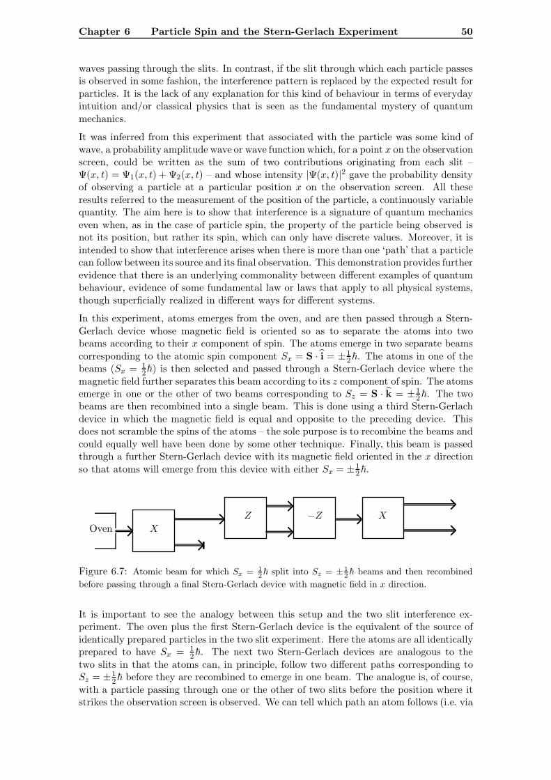
Chapter 6 Particle Spin and the Stern-Gerlach Experiment 50
waves passing through the slits. In contrast, if the slit through which each particle passesis observed in some fashion, the interference pattern is replaced by the expected result forparticles. It is the lack of any explanation for this kind of behaviour in terms of everydayintuition and/or classical physics that is seen as the fundamental mystery of quantummechanics.
It was inferred from this experiment that associated with the particle was some kind ofwave, a probability amplitude wave or wave function which, for a point x on the observationscreen, could be written as the sum of two contributions originating from each slit –Ψ(x, t) = Ψ1(x, t) + Ψ2(x, t) – and whose intensity |Ψ(x, t)|2 gave the probability densityof observing a particle at a particular position x on the observation screen. All theseresults referred to the measurement of the position of the particle, a continuously variablequantity. The aim here is to show that interference is a signature of quantum mechanicseven when, as in the case of particle spin, the property of the particle being observed isnot its position, but rather its spin, which can only have discrete values. Moreover, it isintended to show that interference arises when there is more than one ‘path’ that a particlecan follow between its source and its final observation. This demonstration provides furtherevidence that there is an underlying commonality between different examples of quantumbehaviour, evidence of some fundamental law or laws that apply to all physical systems,though superficially realized in different ways for different systems.
In this experiment, atoms emerges from the oven, and are then passed through a Stern-Gerlach device whose magnetic field is oriented so as to separate the atoms into twobeams according to their x component of spin. The atoms emerge in two separate beamscorresponding to the atomic spin component Sx = S · i = ±1
2�. The atoms in one of thebeams (Sx = 1
2�) is then selected and passed through a Stern-Gerlach device where themagnetic field further separates this beam according to its z component of spin. The atomsemerge in one or the other of two beams corresponding to Sz = S · k = ±1
2�. The twobeams are then recombined into a single beam. This is done using a third Stern-Gerlachdevice in which the magnetic field is equal and opposite to the preceding device. Thisdoes not scramble the spins of the atoms – the sole purpose is to recombine the beams andcould equally well have been done by some other technique. Finally, this beam is passedthrough a further Stern-Gerlach device with its magnetic field oriented in the x directionso that atoms will emerge from this device with either Sx = ±1
2�.
Oven X
Z −Z X
Figure 6.7: Atomic beam for which Sx = 12� split into Sz = ±1
2� beams and then recombinedbefore passing through a final Stern-Gerlach device with magnetic field in x direction.
It is important to see the analogy between this setup and the two slit interference ex-periment. The oven plus the first Stern-Gerlach device is the equivalent of the source ofidentically prepared particles in the two slit experiment. Here the atoms are all identicallyprepared to have Sx = 1
2�. The next two Stern-Gerlach devices are analogous to thetwo slits in that the atoms can, in principle, follow two different paths corresponding toSz = ±1
2� before they are recombined to emerge in one beam. The analogue is, of course,with a particle passing through one or the other of two slits before the position where itstrikes the observation screen is observed. We can tell which path an atom follows (i.e. via
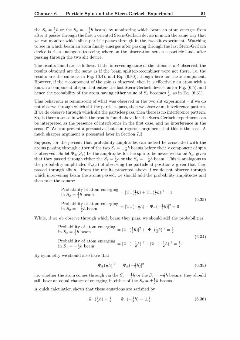
Chapter 6 Particle Spin and the Stern-Gerlach Experiment 51
the Sz = 12� or the Sz = −1
2� beam) by monitoring which beam an atom emerges fromafter it passes through the first z oriented Stern-Gerlach device in much the same way thatwe can monitor which slit a particle passes through in the two slit experiment. Watchingto see in which beam an atom finally emerges after passing through the last Stern-Gerlachdevice is then analogous to seeing where on the observation screen a particle lands afterpassing through the two slit device.
The results found are as follows. If the intervening state of the atoms is not observed, theresults obtained are the same as if the beam splitter-recombiner were not there, i.e. theresults are the same as in Fig. (6.4), and Eq. (6.30), though here for the x component.However, if the z component of the spin is observed, then it is effectively an atom with aknown z component of spin that enters the last Stern-Gerlach device, as for Fig. (6.5), andhence the probability of the atom having either value of Sx becomes 1
2 , as in Eq. (6.31).
This behaviour is reminiscent of what was observed in the two slit experiment – if we donot observe through which slit the particles pass, then we observe an interference pattern.If we do observe through which slit the particles pass, then there is no interference pattern.So, is there a sense in which the results found above for the Stern-Gerlach experiment canbe interpreted as the presence of interference in the first case, and no interference in thesecond? We can present a persuasive, but non-rigorous argument that this is the case. Amuch sharper argument is presented later in Section 7.3.
Suppose, for the present that probability amplitudes can indeed be associated with theatoms passing through either of the two Sz = ±1
2� beams before their x component of spinis observed. So let Ψ±(Sx) be the amplitudes for the spin to be measured to be Sx, giventhat they passed through either the Sz = 1
2� or the Sz = −12� beam. This is analogous to
the probability amplitudes Ψn(x) of observing the particle at position x given that theypassed through slit n. From the results presented above if we do not observe throughwhich intervening beam the atoms passed, we should add the probability amplitudes andthen take the square:
Probability of atom emergingin Sx = 1
2� beam = |Ψ+( 12�) + Ψ−( 1
2�)|2 = 1
Probability of atom emergingin Sx = −1
2� beam = |Ψ+(−12�) + Ψ−(−1
2�)|2 = 0
(6.33)
While, if we do observe through which beam they pass, we should add the probabilities:
Probability of atom emergingin Sx = 1
2� beam = |Ψ+( 12�)|2 + |Ψ−( 1
2�)|2 = 12
Probability of atom emergingin Sx = −1
2� beam = |Ψ+(−12�)|2 + |Ψ−(−1
2�)|2 = 12 .
(6.34)
By symmetry we should also have that
|Ψ±( 12�)|2 = |Ψ±(−1
2�)|2 (6.35)
i.e. whether the atom comes through via the Sz = 12� or the Sz = −1
2� beams, they shouldstill have an equal chance of emerging in either of the Sx = ±1
2� beams.
A quick calculation shows that these equations are satisfied by
Ψ±( 12�) = 1
2 Ψ±(−12�) = ±1
2 . (6.36)
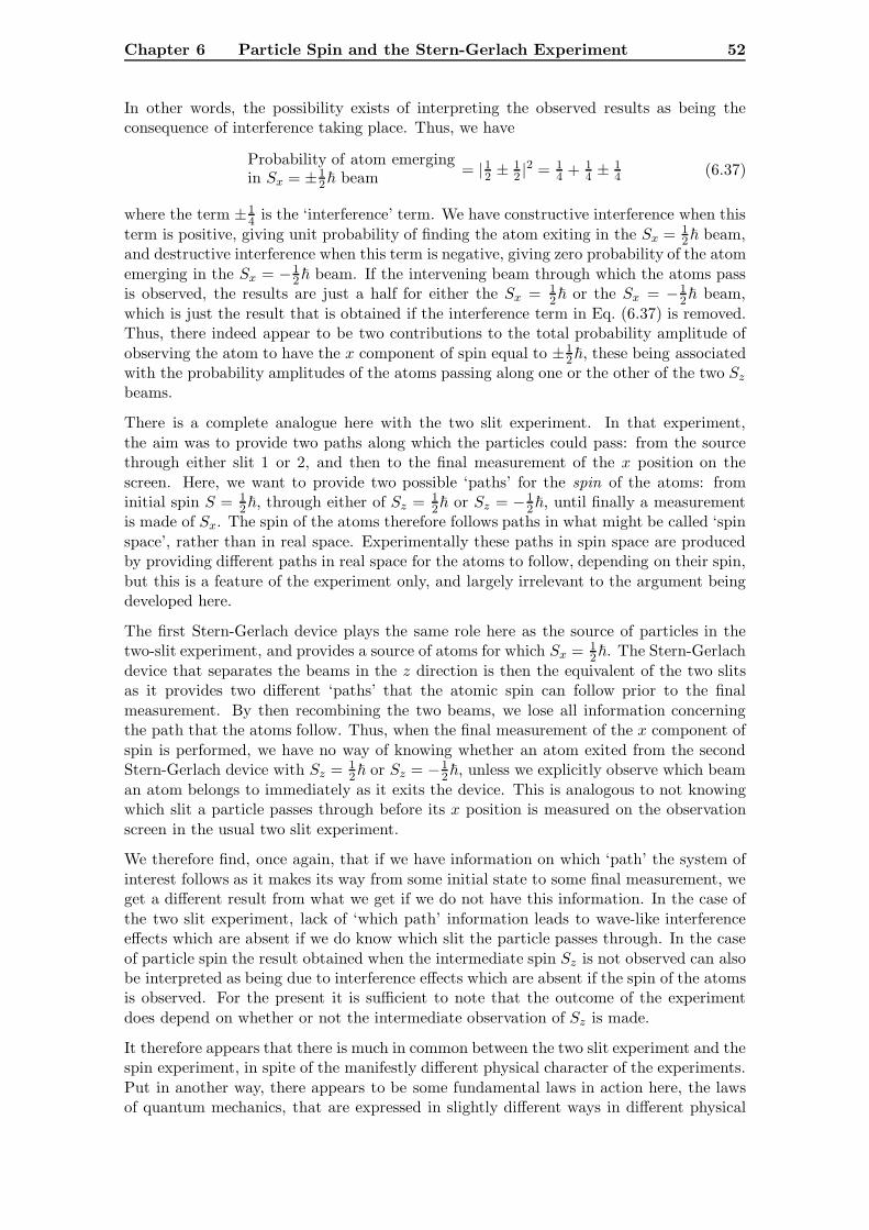
Chapter 6 Particle Spin and the Stern-Gerlach Experiment 52
In other words, the possibility exists of interpreting the observed results as being theconsequence of interference taking place. Thus, we have
Probability of atom emergingin Sx = ±1
2� beam = | 12 ±12 |
2 = 14 + 1
4 ±14 (6.37)
where the term ±14 is the ‘interference’ term. We have constructive interference when this
term is positive, giving unit probability of finding the atom exiting in the Sx = 12� beam,
and destructive interference when this term is negative, giving zero probability of the atomemerging in the Sx = −1
2� beam. If the intervening beam through which the atoms passis observed, the results are just a half for either the Sx = 1
2� or the Sx = −12� beam,
which is just the result that is obtained if the interference term in Eq. (6.37) is removed.Thus, there indeed appear to be two contributions to the total probability amplitude ofobserving the atom to have the x component of spin equal to ±1
2�, these being associatedwith the probability amplitudes of the atoms passing along one or the other of the two Szbeams.
There is a complete analogue here with the two slit experiment. In that experiment,the aim was to provide two paths along which the particles could pass: from the sourcethrough either slit 1 or 2, and then to the final measurement of the x position on thescreen. Here, we want to provide two possible ‘paths’ for the spin of the atoms: frominitial spin S = 1
2�, through either of Sz = 12� or Sz = −1
2�, until finally a measurementis made of Sx. The spin of the atoms therefore follows paths in what might be called ‘spinspace’, rather than in real space. Experimentally these paths in spin space are producedby providing different paths in real space for the atoms to follow, depending on their spin,but this is a feature of the experiment only, and largely irrelevant to the argument beingdeveloped here.
The first Stern-Gerlach device plays the same role here as the source of particles in thetwo-slit experiment, and provides a source of atoms for which Sx = 1
2�. The Stern-Gerlachdevice that separates the beams in the z direction is then the equivalent of the two slitsas it provides two different ‘paths’ that the atomic spin can follow prior to the finalmeasurement. By then recombining the two beams, we lose all information concerningthe path that the atoms follow. Thus, when the final measurement of the x component ofspin is performed, we have no way of knowing whether an atom exited from the secondStern-Gerlach device with Sz = 1
2� or Sz = −12�, unless we explicitly observe which beam
an atom belongs to immediately as it exits the device. This is analogous to not knowingwhich slit a particle passes through before its x position is measured on the observationscreen in the usual two slit experiment.
We therefore find, once again, that if we have information on which ‘path’ the system ofinterest follows as it makes its way from some initial state to some final measurement, weget a different result from what we get if we do not have this information. In the case ofthe two slit experiment, lack of ‘which path’ information leads to wave-like interferenceeffects which are absent if we do know which slit the particle passes through. In the caseof particle spin the result obtained when the intermediate spin Sz is not observed can alsobe interpreted as being due to interference effects which are absent if the spin of the atomsis observed. For the present it is sufficient to note that the outcome of the experimentdoes depend on whether or not the intermediate observation of Sz is made.
It therefore appears that there is much in common between the two slit experiment and thespin experiment, in spite of the manifestly different physical character of the experiments.Put in another way, there appears to be some fundamental laws in action here, the lawsof quantum mechanics, that are expressed in slightly different ways in different physical

Chapter 6 Particle Spin and the Stern-Gerlach Experiment 53
systems: interference and randomness observed in the measurement of particle position inthe two slit experiment, and similar behaviour in the measurement of particle spin. Thelaws of quantum mechanics, and the mathematical language in terms of which these lawsare stated, is the subject of the following Chapter.
Chapter 7
Probability Amplitudes
Evidence was presented in the preceding Chapter that under certain circumstances phys-ical systems of quite disparate nature, but usually on the atomic scale, have the commonproperties of randomness and interference effects, that have no classical explanation. Thesegeneral properties are the indicators, or the signatures, of the existence of basic physicallaws that are not part of our normal everyday view of the way the world behaves, whichimmediately poses the problem of determining, and clearly stating, what these funda-mental laws are. But there is in fact a second problem that has to be dealt with here.In order to state these basic laws, the question arises as to whether or not the conceptsand mathematical language of classical physics is adequate for the task. We have seenthat the mathematics of waves works fine for particles moving through space: from thewave function, which can be derived by solving the Schrodinger equation, informationon the position and momentum, angular momentum, energy, and much else besides canbe obtained. But we have also seen that the wave function cannot be used to describespin. Apart from anything else, spin is a discrete variable, with a finite number of values,unlike the position of a particle which can vary in a continuous way. So what is neededis a mathematical language in terms of which these laws can be expressed, but whichcan assume outwardly different forms when applied to different physical systems. Thetwo problems are not independent: the process of determining what the physical laws areguides us in the development of the mathematical language needed to express these laws.The outcome of all this, in another example of what has been termed ‘the unreasonableeffectiveness of mathematics in physics’ is a mathematical language that was already wellknown to mathematicians in the early days of the quantum theory: the mathematics oflinear vector spaces. It was a British theoretical physicist, Paul Dirac, who played a majorrole in formulating quantum mechanics in this way. He was inspired to do so, in part,because of the above-mentioned need for a theory that could cope with both particle spinand particle motion through space. What this work does, amongst other things, is bringinto sharp focus the problem of defining what is meant by the state of a quantum system,and how a quantum state is to be represented mathematically. A further consequence ofhis work is a succinct notation which encapsulates both the physics and the mathematics,the Dirac bra-ket notation which is used, amongst other things, to represent the state ofa quantum system. The first issue to be dealt with here is then that of coming to termswith what we mean by the state of a system, following which we look again at the two-slitexperiment, which sets the scene for the development of the Dirac/Feynman version ofquantum mechanics.
Chapter 7 Probability Amplitudes 55
7.1 The State of a System
The notion of the state of a system is a central one in both classical and quantum physics,though it is often possible to live with only an intuitive idea of what it means. However,it proves to be important here to have the concept of the state of a system clearly de-fined. Ideally, specifying the state of a system would amount to gathering together allthe information that it is possible to know about the system at any instant in time. Theinformation should be enough so that, in principle, it would be possible to reconstructthe system at some other time and place and have the reconstructed system behave inexactly the same way as the original. From the point of view of physics, this informationwould take the form of numerical data that specifies, for instance for a single particle, itsposition and momentum at any instant in time. Of course, many systems when consideredin all their detail are forbiddingly complex, but fortunately it is not always necessary tospecify everything about a system. For instance, if we are interested in describing theorbit of the Earth around the sun, it would be sufficient to specify the state only in so faras the position and momentum of the centre of mass of the Earth. The fact that the Earthrotates, or that grass is green is not information that is required to deal with the orbitaldynamics of the Earth. Knowing what is relevant and what is not is important in settingup good models of complex systems, but given that this has been decided upon for a givensystem, a good definition of the state of the system consistent with our intuitive notionsis then to say that the state of a system is defined by specifying the maximum amountof data that can, in principle, be known simultaneously without mutual interference orcontradiction about the system.
According to classical physics, it is possible in principle, if not always in practice, todetermine exactly all the quantities needed to specify the state of a physical system.Thus, for a system consisting of a single particle, the state of the system is specified bygiving the position and the momentum of the particle at the instant of interest. For amulti-particle system, the state could be specified by giving the positions and momenta ofthe individual particles, or else, if there are constraints of some kind, e.g. if the particlesare organized into a single rigid body then it is probably sufficient to give the position andmomentum of the centre of mass, the orientation of the body, and a few other quantitiessuch as the linear and angular momentum. In practice, of course, there will always beuncertainty in our knowledge of these quantities, but this can be put down to inadequaciesin our experimental technique, measuring apparatus, or the sheer size and complexity ofthe system under consideration.
When it comes to actually representing the state of a classical system, there is no wayof doing this that has any significance beyond simply being a list of the values of allthe physical parameters that can be determined for the system, though different waysof presenting this information offer different advantages in different circumstances. Anexample of one way of representing the information is, for a single particle, to plot theposition and momentum of the particle as a point (x, p) in what is known as phase space.As a function of time, this point will trace out a path in phase space, this path thenrepresenting the evolution of the state of the system as a function of time.
The situation is somewhat different when quantum effects become important. It is notpossible, even in principle, to specify the position and the momentum of a particle withtotal precision. The uncertainty principle tells us that we either have to compromiseon the accuracy with which we specify each of the quantities, or else have to deal withthe consequences of knowing, say, the position exactly, implying that the momentum istotally unknown, or vice versa. So what then are we to do with the notion of the state ofa quantum particle? The situation is one of accepting the information that we have about
Chapter 7 Probability Amplitudes 56
the system, and taking that as specifying the state, which is consistent with the definitionof state presented above, and is a reflection of what knowledge will really do possess aboutthe system without mutual interference or contradiction. Thus, we can specify the positionof a particle, but not its momentum, so we cannot represent the state of the system inthe same way that we can for a classical system, as a point in phase space, for instance.Similarly we can only specify one component of the spin of a particle, say the x componentof the spin of a particle, in which case we cannot specify its y or z component.
In the next Section we will find it useful to introduce a new notation for the state ofa quantum system, which turns out to be very useful in describing the mathematicalproperties of quantum systems. For the present we will simply introduce the notation asnothing more than a fancy way of writing down all the information that we can knowabout a quantum system. It will look like this:∣∣∣ All the data concerning the system that can be known
without mutual interference or contradiction.
⟩(7.1)
The symbol | 〉 is known as a ket. Contained within the ket is a summary of the dataspecifying the state of a system, and hence a ket is also referred to as the state of thesystem. Thus, for instance, if we know the position of a particle is x = 3 cm with respectto some origin, then the state would be |x = 3 cm〉. If we know that a particle has a z
component of spin equal to 12�, then the state would be |Sz = 1
2�〉. There would thenbe no such state as |Sx = 1
2�, Sz = 12�〉 since it is not possible to known both Sx and Sz
simultaneously. At this stage there seems to be no point to enclosing the description ofthe state of a system within the symbol | 〉, but, as will be seen later, quantum systemshave the schizophrenic property of behaving as if they are simultaneously in a numberof different states, and the way that this property of quantum systems is representedmathematically is by treating the states of a quantum system as if they are vectors in away that we will be discussing later. Hence the above symbol is also known as a ket vectoror state vector.
At times, when we want to be less specific, we would write |x〉 as being the state in whichthe x position of a particle is known, or |px〉 to be the state in which the x componentof momentum is known, though the value in each case is unspecified. Finally, if we wantto talk about a state without trying to spell out just what it is that is known precisely,i.e. an arbitrary state, we will write |ψ〉 or |φ〉 or some such symbol.
As a companion to this notation we will introduce a second way of writing down what thisstate is: ⟨ All the data concerning the system that can be known
without mutual interference or contradiction.
∣∣∣ . (7.2)
This symbol is known as a bra or bra vector and is equally well a way of representing thestate of a quantum system. The distinction between a bra and a ket lies in the mathematicsof quantum mechanics, which we will be dealing with later.
To see how this notation is motivated and employed, and how it acquires a mathematicalmeaning, we return to the two slit experiment.
7.2 The Two Slit Experiment Revisited
We now want to recast the two slit experiment in a fashion that leads to a new way offormulating quantum mechanics. The argument to be presented here is not meant to be
Chapter 7 Probability Amplitudes 57
rigorous, but more to suggest a way of thinking about quantum mechanics that can bemade more precise, and very general in that it can be applied to any physical system.
The experimental set up will be as before, in Chapter 4. Particles, which have all passedthrough exactly the same preparation procedure and hence are presumably all in the samestate, are produced at a source S. These particles are then incident on a screen in whichthere are two narrow slits, 1 and 2, and beyond this screen is a further screen which theparticles will ultimately strike, the point at which they hit this screen being registered insome way.
Since the particles are all prepared in the same way, they will presumably all be associatedwith the same wave function ΨS which we will assume is unity at the source, i.e.
ΨS(S) = 1. (7.3)
We will not be concerning ourselves with the possible time dependence of the wave functionhere – in effect we are assuming some kind of steady state.
This wave function will propagate through space and at the positions of the two slits willhave values ΨS(n), n =1, 2. These waves will then pass through these slits on their waytowards the observation screen. The task then is to determine the amplitude of the wavesat a point x on the observation screen due to waves that originated at each of the slits. Todo that we will first of all suppose that, if the amplitude of the wave incident on slit 1 isunity, then the resulting wave amplitude at a position x on the screen is Ψ1(x). But sincethe amplitude of the wave at slit 1 is ΨS(1) then it appears reasonable to suppose that wescale up the amplitude of the wave from slit 1 incident on the observation screen at x bythe same factor, i.e. ΨS(1), so that the amplitude of the wave incident on the screen at xwill be ΨS(1)Ψ1(x). Of course, this is an assumption, but it is what is observed for, say,light waves passing through a slit – if the amplitude of a light wave incident on a slit isdoubled, then the amplitude of the wave that emerges from the slit is also doubled. Lightwaves are linear. Probability amplitudes are hence also assumed to be linear.
In a similar way, the amplitude at x due to waves from slit 2 will be ΨS(2)Ψ2(x). Conse-quently, the total amplitude of the wave at x will be
ΨS(x) = ΨS(1)Ψ1(x) + ΨS(2)Ψ2(x) (7.4)
where ΨS(x) is the amplitude of waves at x that originated from the source S. This thenis the probability amplitude of observing a particle at x given that it originated from thesource S, i.e. by the Born interpretation Eq. (4.11), |ΨS(x)|2dx is the probability densityof observing a particle in the region x to x + dx. This result is the same as the onepresented in Eq. (4.10), but here we have expressed this total probability amplitude as asum of two contributions of the form
ΨS(n)Ψn(x) = Probability amplitude of observing the particle at slitn given that it originated from the source S.
× Probability amplitude of observing the particle at xgiven that it originated from slit n.
= Probability amplitude for the particle to pass from thesource S to point x through slit n.
(7.5)
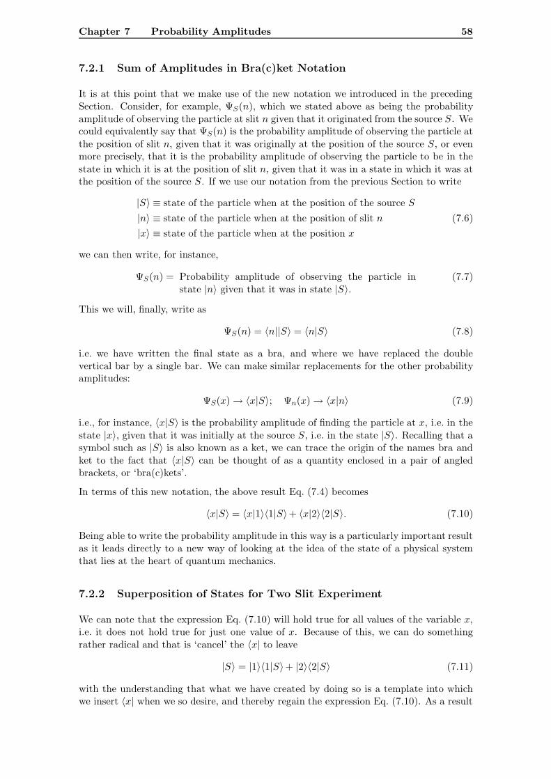
Chapter 7 Probability Amplitudes 58
7.2.1 Sum of Amplitudes in Bra(c)ket Notation
It is at this point that we make use of the new notation we introduced in the precedingSection. Consider, for example, ΨS(n), which we stated above as being the probabilityamplitude of observing the particle at slit n given that it originated from the source S. Wecould equivalently say that ΨS(n) is the probability amplitude of observing the particle atthe position of slit n, given that it was originally at the position of the source S, or evenmore precisely, that it is the probability amplitude of observing the particle to be in thestate in which it is at the position of slit n, given that it was in a state in which it was atthe position of the source S. If we use our notation from the previous Section to write
|S〉 ≡ state of the particle when at the position of the source S|n〉 ≡ state of the particle when at the position of slit n|x〉 ≡ state of the particle when at the position x
(7.6)
we can then write, for instance,
ΨS(n) = Probability amplitude of observing the particle instate |n〉 given that it was in state |S〉.
(7.7)
This we will, finally, write as
ΨS(n) = 〈n||S〉 = 〈n|S〉 (7.8)
i.e. we have written the final state as a bra, and where we have replaced the doublevertical bar by a single bar. We can make similar replacements for the other probabilityamplitudes:
ΨS(x)→ 〈x|S〉; Ψn(x)→ 〈x|n〉 (7.9)
i.e., for instance, 〈x|S〉 is the probability amplitude of finding the particle at x, i.e. in thestate |x〉, given that it was initially at the source S, i.e. in the state |S〉. Recalling that asymbol such as |S〉 is also known as a ket, we can trace the origin of the names bra andket to the fact that 〈x|S〉 can be thought of as a quantity enclosed in a pair of angledbrackets, or ‘bra(c)kets’.
In terms of this new notation, the above result Eq. (7.4) becomes
〈x|S〉 = 〈x|1〉〈1|S〉+ 〈x|2〉〈2|S〉. (7.10)
Being able to write the probability amplitude in this way is a particularly important resultas it leads directly to a new way of looking at the idea of the state of a physical systemthat lies at the heart of quantum mechanics.
7.2.2 Superposition of States for Two Slit Experiment
We can note that the expression Eq. (7.10) will hold true for all values of the variable x,i.e. it does not hold true for just one value of x. Because of this, we can do somethingrather radical and that is ‘cancel’ the 〈x| to leave
|S〉 = |1〉〈1|S〉+ |2〉〈2|S〉 (7.11)
with the understanding that what we have created by doing so is a template into whichwe insert 〈x| when we so desire, and thereby regain the expression Eq. (7.10). As a result
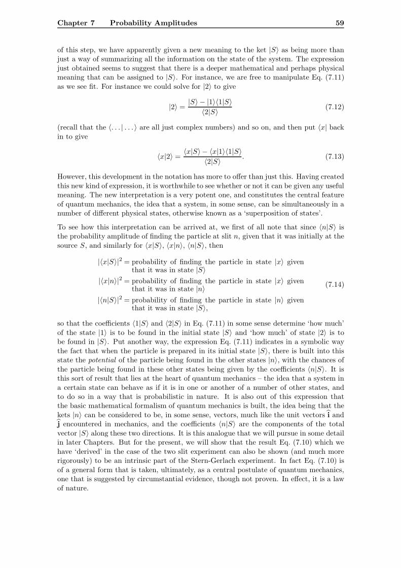
Chapter 7 Probability Amplitudes 59
of this step, we have apparently given a new meaning to the ket |S〉 as being more thanjust a way of summarizing all the information on the state of the system. The expressionjust obtained seems to suggest that there is a deeper mathematical and perhaps physicalmeaning that can be assigned to |S〉. For instance, we are free to manipulate Eq. (7.11)as we see fit. For instance we could solve for |2〉 to give
|2〉 =|S〉 − |1〉〈1|S〉〈2|S〉 (7.12)
(recall that the 〈. . . | . . . 〉 are all just complex numbers) and so on, and then put 〈x| backin to give
〈x|2〉 =〈x|S〉 − 〈x|1〉〈1|S〉
〈2|S〉 . (7.13)
However, this development in the notation has more to offer than just this. Having createdthis new kind of expression, it is worthwhile to see whether or not it can be given any usefulmeaning. The new interpretation is a very potent one, and constitutes the central featureof quantum mechanics, the idea that a system, in some sense, can be simultaneously in anumber of different physical states, otherwise known as a ‘superposition of states’.
To see how this interpretation can be arrived at, we first of all note that since 〈n|S〉 isthe probability amplitude of finding the particle at slit n, given that it was initially at thesource S, and similarly for 〈x|S〉, 〈x|n〉, 〈n|S〉, then
|〈x|S〉|2 = probability of finding the particle in state |x〉 giventhat it was in state |S〉
|〈x|n〉|2 = probability of finding the particle in state |x〉 giventhat it was in state |n〉
|〈n|S〉|2 = probability of finding the particle in state |n〉 giventhat it was in state |S〉,
(7.14)
so that the coefficients 〈1|S〉 and 〈2|S〉 in Eq. (7.11) in some sense determine ‘how much’of the state |1〉 is to be found in the initial state |S〉 and ‘how much’ of state |2〉 is tobe found in |S〉. Put another way, the expression Eq. (7.11) indicates in a symbolic waythe fact that when the particle is prepared in its initial state |S〉, there is built into thisstate the potential of the particle being found in the other states |n〉, with the chances ofthe particle being found in these other states being given by the coefficients 〈n|S〉. It isthis sort of result that lies at the heart of quantum mechanics – the idea that a system ina certain state can behave as if it is in one or another of a number of other states, andto do so in a way that is probabilistic in nature. It is also out of this expression thatthe basic mathematical formalism of quantum mechanics is built, the idea being that thekets |n〉 can be considered to be, in some sense, vectors, much like the unit vectors i andj encountered in mechanics, and the coefficients 〈n|S〉 are the components of the totalvector |S〉 along these two directions. It is this analogue that we will pursue in some detailin later Chapters. But for the present, we will show that the result Eq. (7.10) which wehave ‘derived’ in the case of the two slit experiment can also be shown (and much morerigorously) to be an intrinsic part of the Stern-Gerlach experiment. In fact Eq. (7.10) isof a general form that is taken, ultimately, as a central postulate of quantum mechanics,one that is suggested by circumstantial evidence, though not proven. In effect, it is a lawof nature.
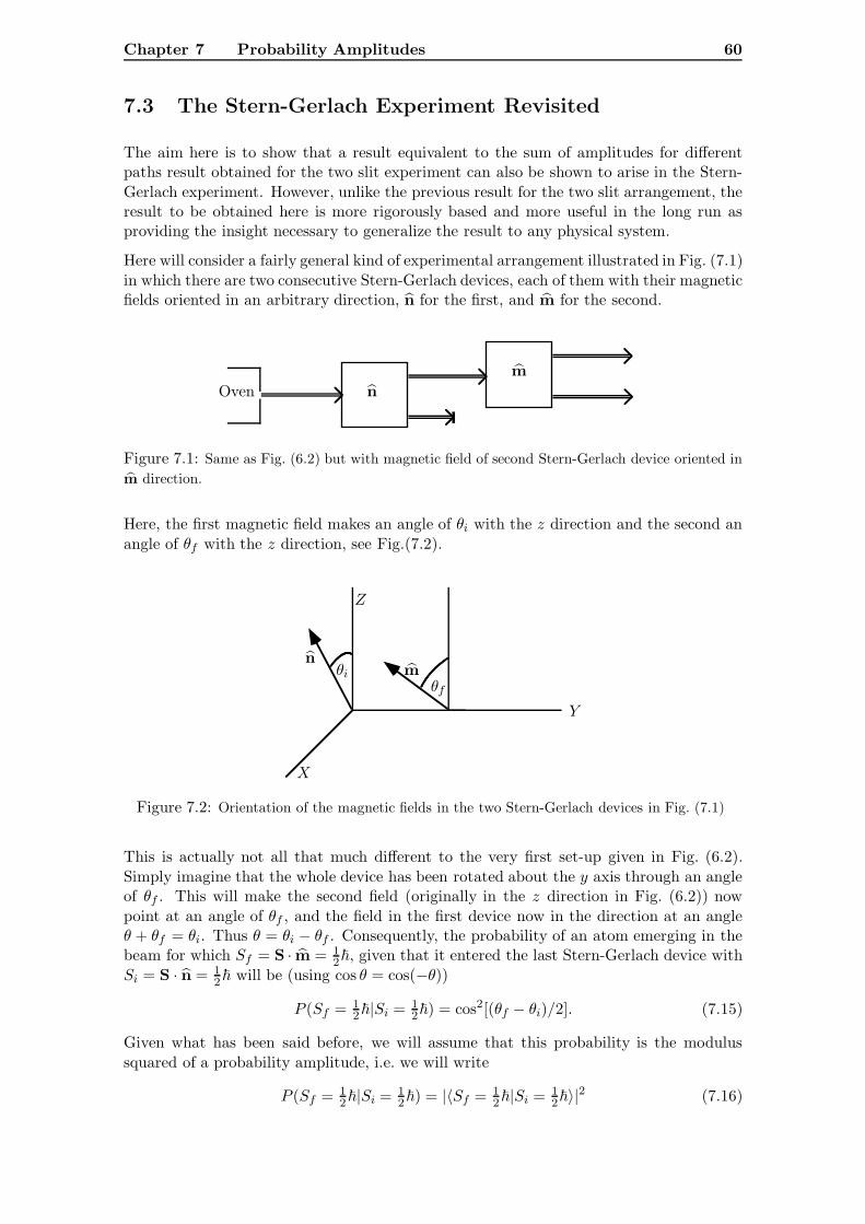
Chapter 7 Probability Amplitudes 60
7.3 The Stern-Gerlach Experiment Revisited
The aim here is to show that a result equivalent to the sum of amplitudes for differentpaths result obtained for the two slit experiment can also be shown to arise in the Stern-Gerlach experiment. However, unlike the previous result for the two slit arrangement, theresult to be obtained here is more rigorously based and more useful in the long run asproviding the insight necessary to generalize the result to any physical system.
Here will consider a fairly general kind of experimental arrangement illustrated in Fig. (7.1)in which there are two consecutive Stern-Gerlach devices, each of them with their magneticfields oriented in an arbitrary direction, n for the first, and m for the second.
nm
Oven
Figure 7.1: Same as Fig. (6.2) but with magnetic field of second Stern-Gerlach device oriented inm direction.
Here, the first magnetic field makes an angle of θi with the z direction and the second anangle of θf with the z direction, see Fig.(7.2).
nm
X
Y
Z
θiθf
Figure 7.2: Orientation of the magnetic fields in the two Stern-Gerlach devices in Fig. (7.1)
This is actually not all that much different to the very first set-up given in Fig. (6.2).Simply imagine that the whole device has been rotated about the y axis through an angleof θf . This will make the second field (originally in the z direction in Fig. (6.2)) nowpoint at an angle of θf , and the field in the first device now in the direction at an angleθ + θf = θi. Thus θ = θi − θf . Consequently, the probability of an atom emerging in thebeam for which Sf = S · m = 1
2�, given that it entered the last Stern-Gerlach device withSi = S · n = 1
2� will be (using cos θ = cos(−θ))
P (Sf = 12�|Si = 1
2�) = cos2[(θf − θi)/2]. (7.15)
Given what has been said before, we will assume that this probability is the modulussquared of a probability amplitude, i.e. we will write
P (Sf = 12�|Si = 1
2�) = |〈Sf = 12�|Si = 1
2�〉|2 (7.16)
Chapter 7 Probability Amplitudes 61
where, following the notation used in the previous Section, 〈Sf = 12�|Si = 1
2�〉 is theprobability amplitude of observing the m component of the spin of an atom to be 1
2�
given that the n component is known to be 12�, or what is equivalent, the probability
amplitude of observing the atom to be in the state |Sf = 12�〉 given that it is initially in
the state |Si = 12�〉. From this, we can write
〈Sf = 12�|Si = 1
2�〉 = eiΦ(θf−θi) cos[(θf − θi)/2] (7.17)
where Φ(θf − θi) is an unknown function which, because it is only the difference in theangular settings of the Stern-Gerlach devices that can be of physical significance, dependsonly on this difference in angles.
We now want to ‘insert’ into this equation the mathematical statement that the atomicspins can pass through some intermediate states which we have the possibility of observing,i.e. by means of an device analogous to the set-up in Fig. (6.7). A general form of thisset-up would involve splitting then recombining the atomic beam in the direction of aunit vector l aligned at some angle θI to the Z axis. Atoms will then emerge with spincomponents SI = S · l that, as usual, can have the two values ±1
2�. If θI = 0, then werecover the situation in Fig. (6.7).
That this possibility is contained in the expression for the probability amplitude Eq. (7.17)can be seen by writing
cos[ 12(θf − θi)] = cos[ 1
2(θf − θI) + 12(θI − θi)]. (7.18)
Using standard trigonometric formulae we get
cos[ 12 (θf − θI) + 1
2 (θI − θi)]= cos[ 1
2 (θf − θI)] cos[ 12(θI − θi)]− sin[ 1
2(θf − θI )] sin[ 12(θI − θi)]. (7.19)
We have generated two terms involving cos factors exactly of the mathematical form thatappears in Eq. (7.17) but in which now appear the angle θI , which we have interpretedabove as specifying the direction l of an intermediate Stern-Gerlach device. These factorscan be readily rewritten in terms of the probability amplitude defined in Eq. (7.17) to give
cos[ 12 (θf − θI)] cos[ 1
2(θI − θi)]= e−iΦ(θf−θI )e−iΦ(θI−θi)〈Sf = 1
2�|SI = 12�〉〈SI = 1
2�|Si = 12�〉. (7.20)
We cannot do this immediately with the terms involving sin, but using simple trigonometrywe can write
sin[ 12(θf − θI)] sin[ 1
2(θI − θi)] = − cos[ 12(θf − (θI + π))] cos[ 1
2((θI + π)− θi)]. (7.21)
Here the intermediate angle is π + θI , which means that l points in exactly the oppositedirection to what it does in Eq. (7.20), so after making the replacement SI → −SI inEq. (7.20) this term becomes
sin[ 12(θf − θI)] sin[ 1
2(θI − θi)]= −e−iΦ(θf −(θI+π))e−iΦ((θI+π)−θi)〈Sf = 1
2�|SI = −12�〉〈SI = −1
2�|Si = 12�〉. (7.22)
Finally, from Eq. (7.17), we have
cos[ 12(θf − θi)] = e−iΦ(θf−θi)〈Sf = 1
2�|Si = 12�〉 (7.23)
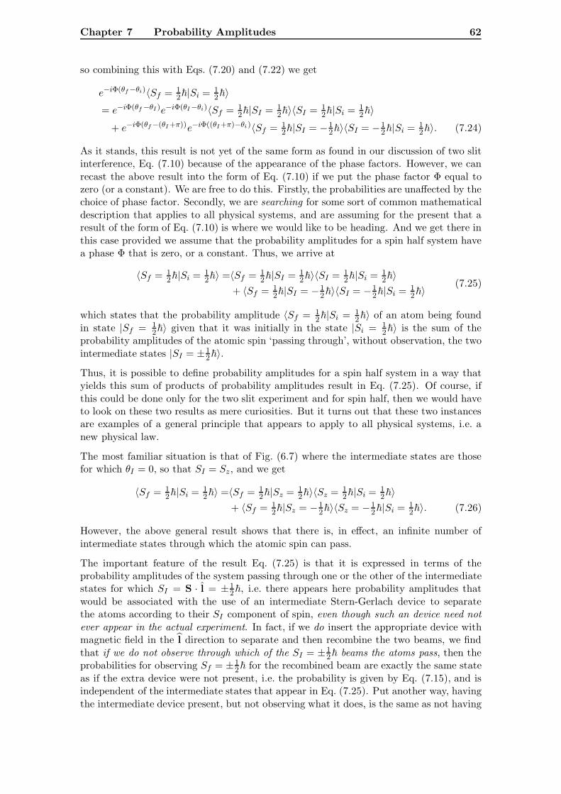
Chapter 7 Probability Amplitudes 62
so combining this with Eqs. (7.20) and (7.22) we get
e−iΦ(θf−θi)〈Sf = 12�|Si = 1
2�〉= e−iΦ(θf −θI )e−iΦ(θI−θi)〈Sf = 1
2�|SI = 12�〉〈SI = 1
2�|Si = 12�〉
+ e−iΦ(θf−(θI+π))e−iΦ((θI+π)−θi)〈Sf = 12�|SI = −1
2�〉〈SI = −12�|Si = 1
2�〉. (7.24)
As it stands, this result is not yet of the same form as found in our discussion of two slitinterference, Eq. (7.10) because of the appearance of the phase factors. However, we canrecast the above result into the form of Eq. (7.10) if we put the phase factor Φ equal tozero (or a constant). We are free to do this. Firstly, the probabilities are unaffected by thechoice of phase factor. Secondly, we are searching for some sort of common mathematicaldescription that applies to all physical systems, and are assuming for the present that aresult of the form of Eq. (7.10) is where we would like to be heading. And we get there inthis case provided we assume that the probability amplitudes for a spin half system havea phase Φ that is zero, or a constant. Thus, we arrive at
〈Sf = 12�|Si = 1
2�〉 =〈Sf = 12�|SI = 1
2�〉〈SI = 12�|Si = 1
2�〉+ 〈Sf = 1
2�|SI = −12�〉〈SI = −1
2�|Si = 12�〉
(7.25)
which states that the probability amplitude 〈Sf = 12�|Si = 1
2�〉 of an atom being foundin state |Sf = 1
2�〉 given that it was initially in the state |Si = 12�〉 is the sum of the
probability amplitudes of the atomic spin ‘passing through’, without observation, the twointermediate states |SI = ±1
2�〉.
Thus, it is possible to define probability amplitudes for a spin half system in a way thatyields this sum of products of probability amplitudes result in Eq. (7.25). Of course, ifthis could be done only for the two slit experiment and for spin half, then we would haveto look on these two results as mere curiosities. But it turns out that these two instancesare examples of a general principle that appears to apply to all physical systems, i.e. anew physical law.
The most familiar situation is that of Fig. (6.7) where the intermediate states are thosefor which θI = 0, so that SI = Sz, and we get
〈Sf = 12�|Si = 1
2�〉 =〈Sf = 12�|Sz = 1
2�〉〈Sz = 12�|Si = 1
2�〉+ 〈Sf = 1
2�|Sz = −12�〉〈Sz = −1
2�|Si = 12�〉. (7.26)
However, the above general result shows that there is, in effect, an infinite number ofintermediate states through which the atomic spin can pass.
The important feature of the result Eq. (7.25) is that it is expressed in terms of theprobability amplitudes of the system passing through one or the other of the intermediatestates for which SI = S · l = ±1
2�, i.e. there appears here probability amplitudes thatwould be associated with the use of an intermediate Stern-Gerlach device to separatethe atoms according to their SI component of spin, even though such an device need notever appear in the actual experiment. In fact, if we do insert the appropriate device withmagnetic field in the l direction to separate and then recombine the two beams, we findthat if we do not observe through which of the SI = ±1
2� beams the atoms pass, then theprobabilities for observing Sf = ±1
2� for the recombined beam are exactly the same stateas if the extra device were not present, i.e. the probability is given by Eq. (7.15), and isindependent of the intermediate states that appear in Eq. (7.25). Put another way, havingthe intermediate device present, but not observing what it does, is the same as not having
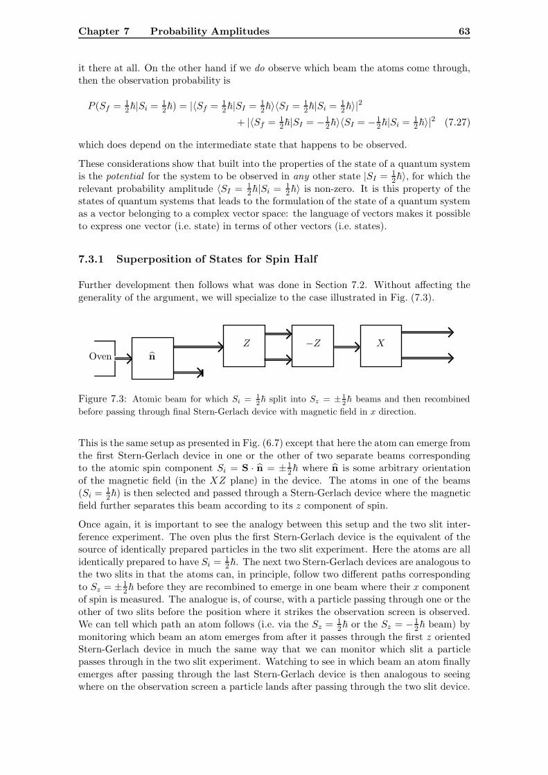
Chapter 7 Probability Amplitudes 63
it there at all. On the other hand if we do observe which beam the atoms come through,then the observation probability is
P (Sf = 12�|Si = 1
2�) = |〈Sf = 12�|SI = 1
2�〉〈SI = 12�|Si = 1
2�〉|2
+ |〈Sf = 12�|SI = −1
2�〉〈SI = −12�|Si = 1
2�〉|2 (7.27)
which does depend on the intermediate state that happens to be observed.
These considerations show that built into the properties of the state of a quantum systemis the potential for the system to be observed in any other state |SI = 1
2�〉, for which therelevant probability amplitude 〈SI = 1
2�|Si = 12�〉 is non-zero. It is this property of the
states of quantum systems that leads to the formulation of the state of a quantum systemas a vector belonging to a complex vector space: the language of vectors makes it possibleto express one vector (i.e. state) in terms of other vectors (i.e. states).
7.3.1 Superposition of States for Spin Half
Further development then follows what was done in Section 7.2. Without affecting thegenerality of the argument, we will specialize to the case illustrated in Fig. (7.3).
Oven nZ −Z X
Figure 7.3: Atomic beam for which Si = 12� split into Sz = ±1
2� beams and then recombined
before passing through final Stern-Gerlach device with magnetic field in x direction.
This is the same setup as presented in Fig. (6.7) except that here the atom can emerge fromthe first Stern-Gerlach device in one or the other of two separate beams correspondingto the atomic spin component Si = S · n = ±1
2� where n is some arbitrary orientationof the magnetic field (in the XZ plane) in the device. The atoms in one of the beams(Si = 1
2�) is then selected and passed through a Stern-Gerlach device where the magneticfield further separates this beam according to its z component of spin.
Once again, it is important to see the analogy between this setup and the two slit inter-ference experiment. The oven plus the first Stern-Gerlach device is the equivalent of thesource of identically prepared particles in the two slit experiment. Here the atoms are allidentically prepared to have Si = 1
2�. The next two Stern-Gerlach devices are analogous tothe two slits in that the atoms can, in principle, follow two different paths correspondingto Sz = ±1
2� before they are recombined to emerge in one beam where their x componentof spin is measured. The analogue is, of course, with a particle passing through one or theother of two slits before the position where it strikes the observation screen is observed.We can tell which path an atom follows (i.e. via the Sz = 1
2� or the Sz = −12� beam) by
monitoring which beam an atom emerges from after it passes through the first z orientedStern-Gerlach device in much the same way that we can monitor which slit a particlepasses through in the two slit experiment. Watching to see in which beam an atom finallyemerges after passing through the last Stern-Gerlach device is then analogous to seeingwhere on the observation screen a particle lands after passing through the two slit device.
Chapter 7 Probability Amplitudes 64
We want to analyze this experiment in a way that is analogous to the two slit experiment.Thus, we are assuming that all the atoms are prepared such that Si = S · n = 1
2� priorto entering the first Stern-Gerlach device. We will then assign a probability amplitude foran atom to pass along either of the Sz = ±1
2� beams, written:
〈Sz = ±12�|Si = 1
2�〉 = Probability amplitude of observing the atom to haveSz = ±1
2� given that originally it had an n componentof spin Si = 1
2�.
=〈±|S〉
(7.28)
where we have simplified the notation a little: 〈Sz = ±12�|Si = 1
2�〉 → 〈±|S〉. The atomsare then recombined and finally, after passing through the last Stern-Gerlach device, willemerge with Sx = ±1
2�. We will then write
〈Sx = ±12�|Sz = 1
2�〉 = Probability amplitude of observing the atom to haveSx = ±1
2� given that it had a z component of spinSz = 1
2�.
=〈S ′|+〉
(7.29)
with a similar definition of 〈Sx = ±12�|Sz = −1
2�〉 → 〈S ′|−〉 where S ′ can have the valuesof ±1
2�. We can then construct the probability amplitude of measuring the x componentof spin to have the value S ′ given that it initially the n component of spin S · n = S = 1
2�
either by analogy with what applied in the two slit experiment, or by use of the moregeneral argument of Section 7.3. Either way, this probability amplitude is given by
〈S ′|S〉 = 〈S ′|+〉〈+|S〉+ 〈S ′|−〉〈−|S〉. (7.30)
Proceeding as in the two slit result, we can argue that this is a reuslt that holds for allfinal states |S ′〉, so that we might as well ‘cancel’ the common factor ‘〈S ′|’ in Eq. (7.30)to give a new expression for the state |S〉, that is
|S〉 = |+〉〈+|S〉+ |−〉〈−|S〉. (7.31)
with the understanding that we can reintroduce ‘〈S ′|’ for any chosen final state, yielding anexpression for the probability amplitudes as needed. What Eq. (7.31) effectively representsis a ‘template’ into which we insert the appropriate information in order to recover therequired probability amplitudes.
We have once again shown how the state of a physical system can, in a sense, be expressedin terms of other possible states of the system, with a weighting that determines the prob-ability of observing the system in each of these other states. To see how this interpretationcan be arrived at, we first of all note that since 〈±|S〉 is the probability amplitude of thez component of spin having the values ±1
2� given that it initially the n component of spinwas S = 1
2�, and similarly for 〈S ′|S〉, 〈S ′|±〉, 〈±|S〉, then
|〈S ′|S〉|2 = probability of the atomic spin being in state |S ′〉 giventhat it was in state |S〉
|〈S ′|±〉|2 = probability of the atomic spin being in the state |S ′〉given that it was in state |±〉
|〈±|S〉|2 = probability of the atomic spin being in the state |±〉given that it was in state |S〉,
(7.32)
Chapter 7 Probability Amplitudes 65
so that the coefficients 〈+|S〉 and 〈−|S〉 in Eq. (7.31) in some sense determine ‘how much’of the state |+〉 is to be found in the initial state |S〉 and ‘how much’ of state |−〉 is tobe found in |S〉. Put another way, the expression Eq. (7.31) indicates in a symbolic waythe fact that when the atomic spin is prepared in its initial state |S〉, there is built intothis state the potential of the spin to be found in the other states |±〉, with the chances ofthe particle being found in these other states being given by the coefficients 〈±|S〉. Onceagain, we see the possibility of a system in a certain state behaving as if it is in one oranother of a number of other states, and to do so in a way that is probabilistic in nature.
Example 7.1 Experiment shows that if an atom is prepared in a state where S = S · i =Sx = 1
2� passes through a Stern-Gerlach device with a magnetic field in the z direction, ithas an equal probability of exiting with either Sz = 1
2� or Sz = −12�. In other words we
have, with |S〉 = |Sx = 12�〉:
|〈±|S〉|2 = 12
so that
〈±|S〉 =1√2eiφ±
where φ± are unknown phase factors. Thus, we have
|S〉 =eiφ+
√2|+〉+
eiφ−√2|−〉.
We need more information to work out what the phase factors are. We cannot do thishere, but what is found is that
|S〉 = e−iφ1√2
[|+〉+ |−〉
].
The last remaining phase factor remains indeterminate. We can choose any value forit without affecting the results of any calculations of physically measurable quantities,something that we cannot show just yet. We shall see this indeterminate phase factoremerge on many occasions.
This result, i.e. that the state of a quantum system can be expressed in the manner ofEq. (7.31) has come about because of the ‘summing over probability amplitudes’ rule illus-trated here using the spin half system as an example. The same mathematical structureappearing in Eq. (7.31) is assumed to arise in the description of all physical systems, i.e. itrepresents a ‘law of nature’ which ultimately leads to considering the quantum state of asystem as an abstract vector in some kind of vector space, a mathematical language thatallows for the possibility, realized physically, that a system in a given state can behave asif it is in some sense made up of other distinct states.
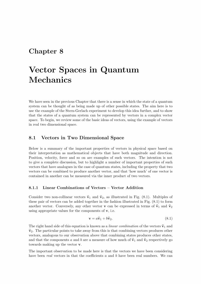
Chapter 8
Vector Spaces in QuantumMechanics
We have seen in the previous Chapter that there is a sense in which the state of a quantumsystem can be thought of as being made up of other possible states. The aim here is touse the example of the Stern-Gerlach experiment to develop this idea further, and to showthat the states of a quantum system can be represented by vectors in a complex vectorspace. To begin, we review some of the basic ideas of vectors, using the example of vectorsin real two dimensional space.
8.1 Vectors in Two Dimensional Space
Below is a summary of the important properties of vectors in physical space based ontheir interpretation as mathematical objects that have both magnitude and direction.Position, velocity, force and so on are examples of such vectors. The intention is notto give a complete discussion, but to highlight a number of important properties of suchvectors that have analogues in the case of quantum states, including the property that twovectors can be combined to produce another vector, and that ‘how much’ of one vector iscontained in another can be measured via the inner product of two vectors.
8.1.1 Linear Combinations of Vectors – Vector Addition
Consider two non-collinear vectors v1 and v2, as illustrated in Fig. (8.1). Multiples ofthese pair of vectors can be added together in the fashion illustrated in Fig. (8.1) to formanother vector. Conversely, any other vector v can be expressed in terms of v1 and v2
using appropriate values for the components of v, i.e.
v = av1 + bv2. (8.1)
The right hand side of this equation is known as a linear combination of the vectors v1 andv2. The particular points to take away from this is that combining vectors produces othervectors, analogous to our observation above that combining states produces other states,and that the components a and b are a measure of how much of v1 and v2 respectively gotowards making up the vector v.
The important observation to be made here is that the vectors we have been consideringhave been real vectors in that the coefficients a and b have been real numbers. We can
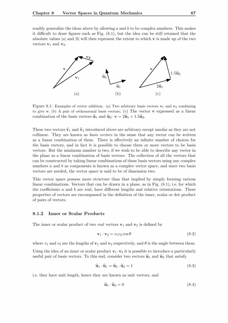
Chapter 8 Vector Spaces in Quantum Mechanics 67
readily generalize the ideas above by allowing a and b to be complex numbers. This makesit difficult to draw figures such as Fig. (8.1), but the idea can be still retained that theabsolute values |a| and |b| will then represent the extent to which v is made up of the twovectors v1 and v2.
v1
v2
v
u1
u2
2u1
1.5u2
v
(a) (b) (c)
Figure 8.1: Examples of vector addition. (a) Two arbitrary basis vectors v1 and v2 combiningto give v; (b) A pair of orthonormal basis vectors; (c) The vector v expressed as a linearcombination of the basis vectors u1 and u2: v = 2u1 + 1.5u2.
These two vectors v1 and v2 introduced above are arbitrary except insofar as they are notcollinear. They are known as basis vectors in the sense that any vector can be writtenas a linear combination of them. There is effectively an infinite number of choices forthe basis vectors, and in fact it is possible to choose three or more vectors to be basisvectors. But the minimum number is two, if we wish to be able to describe any vector inthe plane as a linear combination of basis vectors. The collection of all the vectors thatcan be constructed by taking linear combinations of these basis vectors using any complexnumbers a and b as components is known as a complex vector space, and since two basisvectors are needed, the vector space is said to be of dimension two.
This vector space possess more structure than that implied by simply forming variouslinear combinations. Vectors that can be drawn in a plane, as in Fig. (8.1), i.e. for whichthe coefficients a and b are real, have different lengths and relative orientations. Theseproperties of vectors are encompassed in the definition of the inner, scalar or dot productof pairs of vectors.
8.1.2 Inner or Scalar Products
The inner or scalar product of two real vectors v1 and v2 is defined by
v1 · v2 = v1v2 cos θ (8.2)
where v1 and v2 are the lengths of v1 and v2 respectively, and θ is the angle between them.
Using the idea of an inner or scalar product v1 ·v2 it is possible to introduce a particularlyuseful pair of basis vectors. To this end, consider two vectors u1 and u2 that satisfy
u1 · u1 = u2 · u2 = 1 (8.3)
i.e. they have unit length, hence they are known as unit vectors, and
u1 · u2 = 0 (8.4)
Chapter 8 Vector Spaces in Quantum Mechanics 68
i.e. they are orthogonal. This pair of vectors u1 and u2 is said to be orthonormal. Asbefore, they form a basis in that multiples of each vector can be added together in thefashion illustrated in Fig. (8.1) to form another vector. Conversely, any other vector vcan be expressed using appropriate values for the components of v, i.e.
v = au1 + bu2. (8.5)
The components a and b, which represent ‘how much’ of the vector v is made up of thevectors u1 and u2 are given by
a = u1 · v and b = u2 · v (8.6)
A well known example of a vector expressed as a linear combination of a pair of unitvectors is given by the position vector r written with respect to the unit vectors i and j:
r = xi+ yj. (8.7)
Once again, if we allow for the possibility of complex vectors, then the definition of theinner product is changed to allow for this. Thus the inner product of two vectors v1 andv2 is now v∗1 · v2, and orthonormal vectors satisfy
u∗1 · u1 = u∗2 · u2 = 1u∗1 · u2 = u∗2 · u1 = 0.
(8.8)
Complex basis vectors are not exotic mathematical entities. A simple example is
u1 =3i+ 4ij
5
u2 =4i− 3ij
5(8.9)
though it is true to say that they are not often encountered in mechanics, except at anadvanced level, but are, as we shall see, routinely found in quantum mechanics. Because ofthat, it is convenient to introduce a new notation for inner product (one that is commonlyused on mathematics) which is to write the inner product of two vectors v1 and v2 as(v1, v2), so that we would have here
(v1, v2) = v∗1 · v2. (8.10)
The value of this notation is simply that it is more general and does not tie us to thegeometrical notion of inner product that we are used to using with position vectors, velocityvectors and the like.
8.2 Spin Half Quantum States as Vectors
We now need to examine the way in which the quantum states for a spin half system can beseen to fit in with the idea of being considered as vectors. To see how this comes about, wewill show that there is a perfect analogy between Eqs. (7.30) and (7.31) and correspondingrelationships for ordinary (complex) vectors. Returning to the Stern-Gerlach examplediscussed in the preceding Chapter we obtained there an expression Eq. (7.31)
|S〉 = |+〉〈+|S〉+ |−〉〈−|S〉.
Chapter 8 Vector Spaces in Quantum Mechanics 69
for the state of a spin half atom expressed in terms of the states |±〉, which are statesfor which the atom has a z component of spin equal to ±1
2�, and 〈±|S〉 are probabilityamplitudes (complex numbers) whose magnitude in some sense tells us ‘how much’ of thestates |±〉 are to be found in the state |S〉. This result was obtained by ‘cancelling’ thecommon factor ‘〈S ′|’ from the result
〈S ′|S〉 = 〈S ′|+〉〈+|S〉+ 〈S ′|−〉〈−|S〉.
What we should bear in mind here is that we can recover this relationship between proba-bility amplitudes by reintroducing ‘〈S ′|’ into Eq. (7.31) for any chosen final state, yieldingan expression for the probability amplitudes as needed. Thus, as has been said before,Eq. (7.31) effectively represents a ‘template’ into which we insert the appropriate informa-tion in order to recover the required probability amplitudes. We can also note that thereis nothing sacred about choosing to cancel the the common factor |S〉 – we could equallyas well cancel the factor |S〉, yielding
〈S ′| = 〈S ′|+〉〈+|+ 〈S ′|−〉〈−|. (8.11)
Having carried out this cancellation procedure, what has reappeared is the state of aquantum system i.e. |S〉 which was introduced earlier in a different context, specificallyas being nothing more than a way of writing down all that we knew about the state ofa quantum system. There, the notation had no mathematical significance, but in themanner in which it appears here, it seems to have acquired a mathematical meaning ofsome kind. The aim is to see what this meaning might be, and in doing so, we will showthat the expression for |S〉 has many of the properties that we associate with expressinga vector as a sum of its components.
We begin by considering the probability amplitudes 〈S ′|S〉 themselves. These are complexnumbers in general for arbitrary spin directions, (but they were real in the particular Stern-Gerlach example used above), such that their modulus squared |〈S ′|S〉|2 is the probabilityP (S ′|S) of observing the spin to be in the state |S ′〉 given that it was in the state |S〉. Inparticular, 〈S|S〉 is the probability amplitude of observing the spin to be in the state |S〉given that it was in the state |S〉. This will have to be unity, i.e. P (S|S) = |〈S|S〉|2 = 1.Thus we can conclude that
〈S|S〉 = eiη (8.12)
where η is an arbitrary phase. It turns out that this phase always cancels out in anycalculation of observable quantities, so it is conventionally set to zero, and hence
〈S|S〉= 1. (8.13)
The state |S〉 is said to be normalized to unity.
As a particular case, this last result implies that
〈+|+〉 = 1. (8.14)
We can now consider the probability amplitude 〈+|S〉 obtained by replacing S ′ by + inhe above expression for 〈S ′|S〉:
〈+|S〉 = 〈+|+〉〈+|S〉+ 〈+|−〉〈−|S〉. (8.15)
We have seen that we can put 〈+|+〉 = 1, so we have
〈+|−〉〈−|S〉 = 0 (8.16)
Chapter 8 Vector Spaces in Quantum Mechanics 70
which has to be true no matter what the state |S〉 happens to be, i.e. no matter whatvalue the probability amplitude 〈−|S〉 is. Thus we conclude that
〈+|−〉 = 0. (8.17)
Similarly we can show that
〈−|−〉 = 1 and 〈−|+〉 = 0. (8.18)
Thus we can set up a comparison:
〈+|+〉 = 1〈+|−〉 = 0〈−|−〉 = 1〈−|+〉 = 0
←→←→←→←→
u∗1 · u1 = 1u∗2 · u1 = 0u∗2 · u2 = 1u∗2 · u1 = 0
(8.19)
which implies the following correspondences:
|+〉 ←→ u1 |−〉 ←→ u2
〈+| ←→ u∗1 〈−|←→ u∗2.(8.20)
We know that 〈+|S〉 and 〈−|S〉 are both just complex numbers, so call them a and b
respectively. If we now write
|S〉 = a|+〉+ b|−〉 (8.21)
we establish a perfect correspondence with the expression
v = a u1 + b u2. (8.22)
On the basis of this result, we are then tempted to interpret the ket |S〉 as a vectorexpressed as a linear combination of two orthonormal basis vectors |±〉. We can push theanalogy further if we once again use the fact that 〈S|S〉= 1, so that
〈S|S〉 = 1 = 〈S|−〉〈−|S〉+ 〈S|+〉〈+|S〉 (8.23)
On the other hand, the total probability of observing the system in either of the states|±〉 must add up to unity, which means that
P (+|S) + P (−|S) = |〈+|S〉|2 + |〈−|S〉|2 = 1. (8.24)
By comparing the last two equations, and noting that
|〈±|S〉|2 = 〈±|S〉〈±|S〉∗ (8.25)
we conclude that
〈±|S〉 = 〈S|±〉∗. (8.26)
If we now consider
〈S ′| = 〈S ′|+〉〈+|+ 〈S ′|−〉〈−|
and use the result, Eq. (8.26), 〈±|S ′〉 = 〈S ′|±〉∗, we can write this as
〈S ′| = 〈+|S ′〉∗〈+|+ 〈−|S ′〉∗〈−| (8.27)
Chapter 8 Vector Spaces in Quantum Mechanics 71
or, expressed in terms of a′ = 〈+|S ′〉 and b′ = 〈−|S ′〉, we have
〈S ′| = a′∗〈+|+ b′∗〈−| (8.28)
which has a perfect correspondence with an ordinary vector v′ in the form
v′∗ = a′∗u∗1 + b′∗u∗2. (8.29)
So the bra 〈S ′| is itself a vector, a bra vector, which can be thought of as being just thecomplex conjugate of the corresponding ket vector |S ′〉. But while it is occasionally usefulto think this way, it is not strictly true mathematically, and this way of viewing a bravector will not be employed here. Instead, as will be shown shortly, an interpretation of ketvectors as column vectors leads to the interpretation of bra vectors as row vectors. A moremathematical standpoint also leads to interpretation of bra vectors as ‘linear functionals’,that is, a bra is a mathematical operator that acts on a ket vector to produce a complexnumber.
Finally, to complete the correspondence, we note that the probability amplitude 〈S ′|S〉can be written
〈S ′|S〉 = a′∗a + b′∗b (8.30)
which can be compared with the inner product v′∗ ·v, or written in the more formalnotation:
(v′, v) = a′∗a+ b′∗b (8.31)
which tells us that the probability amplitude can be considered as being simply the innerproduct of the two vectors |S ′〉 and |S〉, i.e.
〈S ′|S〉 = (|S ′〉, |S〉). (8.32)
In other words, we have a perfect analogy between the two dimensional complex vectorspace formed by linear combinations of the unit vectors u1 and u2 discussed in Section8.1 and a complex vector space consisting of all the linear combinations of the states |±〉.The ket vectors |±〉 are referred to as basis states, analogous to u1 and u2 being referredto as basis vectors.
Different spin states can be constructed by forming linear combinations of these basisstates: a|+〉+b|−〉. We have only been looking at linear combinations with real coefficients.This was all that was needed, essentially because we have only been measuring componentsof the total spin S that lie in the same XZ plane. What if the coefficients a and b arecomplex? In this case, it is found that the state |S〉 corresponds to a component S = S ·nfor which n points out of this plane though we will not attempt to prove this here (seeEq. (8.46)). So, any linear combination in which a and b are any complex numbersalso defines a possible spin state of the spin half system. Thus all the possible linearcombinations of |±〉, i.e. combinations of the form a|+〉+ b|−〉 where a and b are complexnumbers form a complex vector space known as the state space of the system.
The quantum state vectors can also be ‘multiplied’ together – the inner product of thetwo vectors |S ′〉 and |S〉 is just the probability amplitude 〈S ′|S〉. In particular, the basisstates are normalized to unity, i.e. they are unit vectors, and they are orthogonal to eachother, i.e. they form a pair of orthonormal basis states.
The terminology often adopted is to say that the state vector |S〉 = a|+〉+b|−〉 is a ‘linearsuperposition’ of the two states |±〉. The probability amplitudes a = 〈+|S〉 and b = 〈−|S〉
Chapter 8 Vector Spaces in Quantum Mechanics 72
represent ‘how much’ of the states |±〉 are contained within the state |S〉 to the extentthat |〈±|S〉|2 is the probability of the z component of spin being found to have the values±1
2�.
One difference between ordinary vectors and quantum state vectors is the importance ofthe ‘normalization condition’, i.e. the requirement that 〈S|S〉 = 1, which must hold truegiven the interpretation of the inner product as a probability amplitude. But how can thisbe reconciled with the statement above that any linear combination of the basis states isa possible state of the system? How can a state vector such as |S〉 = |+〉+ |−〉 which hasthe property
〈S|S〉 = 2 (8.33)
be a physically acceptable state vector as it seems to be saying that the probability offinding the system in the state |S〉 given that it is in the state |S〉 is 4, which does notmake sense. But, if we define a new vector |S〉 by
|S〉 =|S〉√〈S|S〉
=1√2|S〉 (8.34)
then automatically |S〉 will have the required normalization property – it is said to benormalized to unity. So, rather than abandoning giving a physical interpretation of statevectors which are not normalized to unity, the approach adopted is that we can multiplyany state vector by any factor and say that it still represents the same physical state,i.e. |S〉 and |S〉 = a|S〉, where a is any complex number, represent the same physical state.However, it is only the normalized state |S〉 that should be used in any calculations inorder to be certain that probability is properly accounted for.
This can be summarized in a table:
Classical vector Quantum state vector for spinhalf system
Basis Vectors u1, u2 |+〉, |−〉
Inner Product (v1, v2) = v∗1 · v2 (|S ′〉, |S〉) = 〈S ′|S〉
Orthonormality u∗1 · u1 = u∗2 · u2 = 1u∗1 · u2 = u∗2 · u1 = 0
〈+|+〉 = 〈−|−〉 = 1〈+|−〉 = 〈−|+〉 = 0
Linearcombination
v = au1 + bu2
a and b complex numbers|S〉 = a|+〉+ b|−〉a and b complex numbers
Normalisation — 〈S|S〉= 1
A More Detailed Analysis One of the important properties of vectors is that two ormore of them can be combined as a ‘linear combination’ to produce a third. If we are toconsider quantum states as vectors, then this very basic property must also be possessed byquantum states. In the above, we have not really shown that any linear combination of thebasis states |±〉, does indeed represent a possible state of the system, even if we restrictourselves to the case of the measuring spin components in the XZ plane. But a more
Chapter 8 Vector Spaces in Quantum Mechanics 73
detailed argument than that just presented can be used to strengthen this conclusion. Tosee how this comes about, we return to the above expression Eq. (7.25) for the probabilityamplitude 〈Sf = 1
2�|Si = 12�〉:
〈Sf = 12�|Si = 1
2�〉 =〈Sf = 12�|SI = 1
2�〉〈SI = 12�|Si = 1
2�〉+ 〈Sf = 1
2�|SI = −12�〉〈SI = −1
2�|Si = 12�〉.
(8.35)
We can ‘cancel’ 〈Sf = 12�| from this expression and write
|Si = 12�〉 = |SI = 1
2�〉〈SI = 12�|Si = 1
2�〉 + |SI = −12�〉〈SI = −1
2�|Si = 12�〉 (8.36)
In Section 7.3, Eq. (7.17), the quantity 〈Sf = 12�|Si = 1
2�〉 was shown to be given by
〈Sf = 12�|Si = 1
2�〉 = cos[(θf − θi)/2]
with the phase factor exp(iΦ) put equal to unity, and with n and m, the directions of themagnetic fields, confined to the XZ plane. The probability amplitudes for the system topass through the intermediate states |SI = ±1
2�〉, that is, 〈SI = ±12�|Si = 1
2�〉 are likewisegiven by
〈SI = 12�|Si = 1
2�〉 = cos[ 12(θI − θi)]
〈SI = −12�|Si = 1
2�〉 = cos[ 12(θI + π − θi)] = − sin[ 1
2(θI − θi)].(8.37)
so that Eq. (8.36) becomes
|Si = 12�〉 = cos[ 1
2(θI − θi)]|SI = +12�〉 − sin[ 1
2(θI − θi)]|SI = −12�〉. (8.38)
To further simplify things, we will assume that θI = 0, i.e. the l vector is in the z direction.In addition, we will make the notational simplification already used above defined by
|Si = 12�〉 →|S〉
|SI = ±12�〉 →|±〉
〈SI = ±12�|Si = 1
2�〉 →〈±|S〉
so that |±〉 = |Sz = ±12�〉, and Eq. (8.36) becomes
|S〉 = |+〉〈+|S〉+ |−〉〈−|S〉. (8.39)
or, using Eq. (8.37)
|S〉 = cos( 12θi)|+〉+ sin( 1
2θi)|−〉. (8.40)
We are now at the point at which we can begin to supply an interpretation to this equation.What this equation is saying is that the combination cos(1
2θi)|+〉+ sin( 12θi)|−〉, and |S〉,
both represent the same thing – the atomic spin is in a state for which Si = 12�. In other
words, if we were presented with the combination:
1√2|+〉+ 1√
2|−〉 (8.41)
we immediately see that cos( 12θi) = 1/
√2 and sin(1
2θi) = 1/√
2, and hence θi = 90◦. Thusthe magnetic field is pointing in the direction 90◦ to the z direction, i.e. in the x direction,and hence the spin state of the atom is the state |S〉 = |Sx = 1
2�〉.
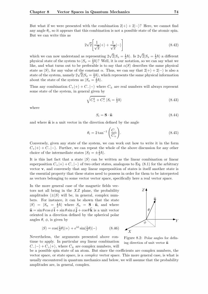
Chapter 8 Vector Spaces in Quantum Mechanics 74
But what if we were presented with the combination 2|+〉 + 2|−〉? Here, we cannot findany angle θi, so it appears that this combination is not a possible state of the atomic spin.But we can write this as
2√
2
[1√2|+〉+
1√2|−〉]
(8.42)
which we can now understand as representing 2√
2|Sx = 12�〉. Is 2
√2|Sx = 1
2�〉 a differentphysical state of the system to |Sx = 1
2�〉? Well, it is our notation, so we can say what welike, and what turns out to be preferable is to say that α|S〉 describes the same physicalstate as |S〉, for any value of the constant α. Thus, we can say that 2|+〉+ 2|−〉 is also astate of the system, namely 2
√2|Sx = 1
2�〉, which represents the same physical informationabout the state of the system as |Sx = 1
2�〉.Thus any combination C+|+〉 + C−|−〉 where C± are real numbers will always representsome state of the system, in general given by√
C2+ +C2
− |Si = 12�〉 (8.43)
where
Si = S · n (8.44)
and where n is a unit vector in the direction defined by the angle
θi = 2 tan−1
(C−C+
). (8.45)
Conversely, given any state of the system, we can work out how to write it in the formC+|+〉 + C−|−〉. Further, we can repeat the whole of the above discussion for any otherchoice of the intermediate states |SI = ±1
2�〉.It is this last fact that a state |S〉 can be written as the linear combination or linearsuperposition C+|+〉+C−|−〉 of two other states, analogous to Eq. (8.1) for the arbitraryvector v, and conversely that any linear superposition of states is itself another state isthe essential property that these states need to possess in order for them to be interpretedas vectors belonging to some vector vector space, specifically here a real vector space.
In the more general case of the magnetic fields vec-tors not all being in the XZ plane, the probabilityamplitudes 〈±|S〉 will be, in general, complex num-bers. For instance, it can be shown that the state|S〉 = |Sn = 1
2�〉 where Sn = S · n, and wheren = sin θ cosφ i+ sin θ sinφ j+ cos θ k is a unit vectororiented in a direction defined by the spherical polarangles θ, φ, is given by
|S〉 = cos( 12θ)|+〉+ eiφ sin( 1
2θ)|−〉 (8.46)
Nevertheless, the arguments presented above con-tinue to apply. In particular any linear combinationC−|−〉+C+|+〉, where C± are complex numbers, will
φ
θ
n
X
Y
Z
Figure 8.2: Polar angles for defin-ing direction of unit vector n
be a possible spin state of an atom. But since the coefficients are complex numbers, thevector space, or state space, is a complex vector space. This more general case, is what isusually encountered in quantum mechanics and below, we will assume that the probabilityamplitudes are, in general, complex.

Chapter 8 Vector Spaces in Quantum Mechanics 75
8.3 The General Case of Many Intermediate States
The above results were based on the particular case of a spin half system which couldpass through two possible intermediate spin states, and was developed, at least in part,by analogy with the two slit experiment where a particle could pass through two possibleintermediate states defined by the positions of the slits. We can generalize these resultsto apply to situations in which the system can pass through any number of intermediatestates, and where the intermediate states can be more general states of quantum systems.So, suppose we have some unspecified system which is prepared initially in some state|ψ〉, and we are interested in finding it in some other state |φ〉. Further suppose that thesystem can pass through any of a set of intermediate states {|ϕn〉; n = 1, 2, . . .} wherethese states form a set of orthonormal basis states, i.e.
〈ϕm|ϕn〉 = δmn = 1 n = m
= 0 n �= m (8.47)
where δmn is known as the Kronecker delta. Then
1. 〈φ|ψ〉 = the probability amplitude of the system being found in the state |φ〉given that it was in state |ψ〉.
2. |〈φ|ψ〉|2 = the probability of the system being found in the state |φ〉 given thatit was in state |ψ〉.
3. The closure relation:
〈φ|ψ〉 =∑n
〈φ|ϕn〉〈ϕn|ψ〉 (8.48)
which tells us that the total probability amplitude of finding the system in the finalstate |φ〉 is just the sum of the probability amplitudes of the system passing throughany of the intermediate states {|ϕn〉; n = 1, 2, . . .}.
4. The completeness relations:
|ψ〉 =∑n
|ϕn〉〈ϕn|ψ〉 (8.49)
〈φ| =∑n
〈φ|ϕn〉〈ϕn| (8.50)
which tells us that either the intial or final states can be expressed as a linearcombination of the intermediate states {|n〉; n = 1, 2, . . .}.
5. 〈φ|ψ〉 = 〈ψ|φ〉∗.
6. The normalization condition:
〈ψ|ψ〉=∑n
〈ψ|ϕn〉〈n|ψ〉 =∑n
|〈ϕn|ψ〉|2 = 1. (8.51)
This last result tells us that the probability of finding the system in any of the states |n〉adds up to unity. Moreover, we know that 〈ϕm|ϕn〉 = 0 if n �= m so that a system instate |ϕn〉 can never be found in some other state |ϕm〉. Consequently, the set of states{|ϕn〉; n = 1, 2, . . .} represent a complete set of possible alternative final states, complete
Chapter 8 Vector Spaces in Quantum Mechanics 76
in the sense that the total probability of ending up in any of the mutually exclusive possiblefinal states |ϕn〉 adds up to unity – there is nowhere else for the system to be found. Thusthe set of states {|ϕn〉; n = 1, 2, . . .} is known as a complete set of orthonormal basis states.It is one of the major tasks in dealing with a quantum system of identifying a set of basisstates.
8.4 General Mathematical Description of a Quantum Sys-
tem
Most of the discussion above has been developed on the basis of studying the properties ofsystems that can pass through different intermediate states, leading to the idea of summingthe probability amplitudes associated with the different ‘paths’ that the system can passalong between the initial and observed final state. The preceding section extended thisperspective to apply to arbitrary systems with arbitrary numbers of intermediate states.
But is was also shown that the mathematical description of this sum of probability ampli-tudes admits an interpretation of the state of the system as being a vector in a complexvector space, the state space of the system. It is this mathematical picture that is sum-marized here. This idea that the state of a quantum system is to be considered a vectorbelonging to a complex vector space, which we have developed here in the case of a spinhalf system, and which has its roots in the sum over paths point of view, is the basis of allof modern quantum mechanics and is used to describe any quantum mechanical system.Below is a summary of the main points as they are used for a general quantum systemwhose state spaces are of arbitrary dimension (including state spaces of infinite dimen-sion). The emphasis here is on the mathematical features of the theory, removing it frombeing couched in the language of probability amplitudes for different intermediate states.
8.4.1 State Space
We have indicated a number of times that in quantum mechanics, the state of a physicalsystem is represented by a vector belonging to a complex vector space known as the statespace of the system. Here we will give a list of the defining conditions of a state space,though we will not be concerning ourselves too much with the formalities.
The following definitions and concepts set up the state space of a quantum system.
1. Every physical state of a quantum system is specified by a vector called a statevector, ket vector, or sometimes just state and written | . . . 〉 where . . . is a labelspecifying the physical information known about the state. An arbitrary state iswritten |ψ〉, or |φ〉 and so on. The set of all state vectors describing a given physicalsystem forms a complex vector space (or Hilbert space) H also known as the statespace or ket space for the system.
2. Every linear superposition of two or more state vectors |φ1〉, |φ2〉, |φ3〉, . . . , is alsoa state of the quantum system i.e. the state |ψ〉 given by
|ψ〉 = c1|φ1〉+ c2|φ2〉+ c3|φ3〉+ . . .
is a state of the system for all complex numbers c1, c2, c3, . . . .
Chapter 8 Vector Spaces in Quantum Mechanics 77
These last two points amount to saying that every physical state of a system is representedby a vector in the state space of the system, and every vector in the state space representsa possible physical state of the system. To guarantee this, the following condition is alsoimposed:
3. If a state of the system is represented by a vector |ψ〉, then the same state is repre-sented by the vector c|ψ〉 where c is any non-zero complex number.
Finally, we need the concept of a set of basis states, and of the dimension of the statespace.
4. A set of vectors {|ϕ1〉, |ϕ2〉, |ϕ3〉, . . .} is said to form a basis for the state space ifevery state of the quantum system can be represented as a linear superposition ofthe |ϕi〉’s i.e. for any state |ψ〉 we can write
|ψ〉 =∑i
ci|ϕi〉.
The set of vectors {|ϕi〉, i = 1, 2, . . .} are said to span the vector space. The vectorsare also termed the base states for the vector space. They are also said to becomplete. The latter means that no more basis states are needed to describe anypossible physical state of a system.
For example, returning to the spin half system, the two states |±〉 are all that is neededto describe any state of the system, i.e. there are no spin states that cannot be describedin terms of these basis states. Thus, these states are said to be complete.
5. The minimum number of vectors needed to form a complete set of basis states isknown as the dimension of the state space. [In many, if not most cases of interest inquantum mechanics, the dimension of the state space is infinite.]
It should be noted that there is an infinite number of possible basis states for any statespace. Often the choice of basis states is suggested by the physics (such as the set ofeigenstates of an observable, see Chapter 9), but even so, it can be convenient to transformfrom one basis state to another.
8.4.2 Probability Amplitudes and the Inner Product of State Vectors
We obtained a number of properties of probability amplitudes when looking at the case ofa spin half system. Some of the results obtained there, and a few more that were not, aresummarized in the following. These conditions on probability amplitudes are identical tothe conditions that define an inner product.
If |φ〉 and |ψ〉 are any two state vectors belonging to the state space H, then
1. 〈φ|ψ〉, a complex number, is the probability amplitude of observing the system tobe in the state |φ〉 given that it is in the state |ψ〉.
2. The probability of observing the system to be in the state |φ〉 given that it is in thestate |ψ〉 is |〈φ|ψ〉|2.
Chapter 8 Vector Spaces in Quantum Mechanics 78
The probability amplitude 〈φ|ψ〉, can then be shown to have the properties
3. 〈φ|ψ〉 = 〈ψ|φ〉∗.
4. (〈φ|{c1|ψ1〉+ c2|ψ2〉} = c1〈φ|ψ1〉+ c2〈φ|ψ2〉 where c1 and c2 are complex numbers.
5. 〈ψ|ψ〉 ≥ 0. If 〈ψ|ψ〉=0 then |ψ〉 = 0, the zero vector.
This last statement is related to the physically reasonable requirement that the probabilityof a system being found in a state |ψ〉 given that it is in the state |ψ〉 has to be unity,i.e. |〈ψ|ψ〉|2 = 1 which means that 〈ψ|ψ〉 = exp(iη). We now choose η = 0 so that〈ψ|ψ〉 = 1, which is bigger than zero. But recall that any multiple of a state vector stillrepresents the same physical state of the system, i.e. |ψ〉 = a|ψ〉 still represents the samephysical state as |ψ〉. However, in this case, 〈ψ|ψ〉 = |a|2 which is not necessarily unity,but is is certainly bigger than zero.
6. The quantity√〈ψ|ψ〉 is known as the length or norm of |φ〉.
7. A state |φ〉 is normalized, or normalized to unity, if 〈φ|φ〉 = 1.
Normalized states are states for which probability is properly taken into account. It ismathematically convenient to permit the use of states whose norms are not equal to unity,it is necessary in order to make use of the probability interpretation to deal only with thatstate which has norm of unity. Any state that cannot be normalized to unity (i.e. it is ofinfinite length) cannot represent a physically acceptable state.
8. Two states |φ〉 and |ψ〉 are orthogonal if 〈φ|ψ〉 = 0.
The physical significance of two states being orthogonal should be understood: for a systemin a certain state, there is zero probability of it being observed in a state with which itis orthogonal. In this sense, two orthogonal states are as distinct as it is possible for twostates to be.
Finally, a set of orthonormal basis vectors {|ϕn〉; n = 1, 2, . . .} will have the property
9. 〈ϕm|ϕn〉 = δmn where δmn is known as the Kronecker delta, and equals unity ifm = n and zero if m �= n.
All the above conditions satisfied by probability amplitudes are identical to the conditionsthat are used to define the inner product of two vectors in the state space, i.e. we couldwrite, using the usual mathematical notation for an inner product, 〈φ|ψ〉 = (|φ〉, |ψ〉).
It is usually required in quantum mechanics that certain convergency criteria, defined interms of the norms of sequences of vectors belonging to the state space, must be satisfied.This is not of any concern for spaces of finite dimension, but are important for spaces ofinfinite dimension. If these criteria are satisfied then the state space is said to be a Hilbertspace. Thus rather than referring to the state space of a system, reference is made to theHilbert space of the system.
Recognizing that a probability amplitude is nothing but an inner product on the statespace of the system, leads to a more general way of defining what is meant by a bravector. The following discussion emphasizes the fact that a bra vector, while it sharesmany characteristices of a ket vector, is actually a different mathematical entity.
Chapter 8 Vector Spaces in Quantum Mechanics 79
Bra Vectors
We have consistently used the notation 〈S ′|S〉 to represent a probability amplitude, but wehave just seen that this quantity is in fact nothing more than the inner product of two statevectors, which can be written in a different notation, (|S ′〉, |S〉), that is more commonlyencountered in pure mathematics. But the inner product can be viewed in another way,which leads to a new interpretation of the expression 〈S ′|S〉, and the introduction of anew class of state vectors.
If we consider the equation
〈S ′|S〉 = (|S ′〉, |S〉) (8.52)
and ‘cancel’ the |S〉, we get the result
〈S ′| • = (|S ′〉, •) (8.53)
where the ‘•’ is inserted, temporarily, to remind us that in order to complete the equation,a ket vector has to be inserted. By carrying out this procedure, we have introduced anew quantity 〈S ′| which is known as a bra or bra vector, essentially because 〈S ′|S〉 lookslike quantities enclosed between a pair of ‘bra(c)kets’. It is a vector because, as can bereadily shown, the collection of all possible bras form a vector space. For instance, by theproperties of the inner product, if
|S〉 = C+|+〉+ C−|−〉 (8.54)
then
(|S〉, •) = 〈S| • = (C+|+〉+C−|−〉, •) (8.55)= C∗
+(|+〉, •) + C∗−(|−〉, •) = C∗
+〈+| •+ C∗−〈−| • (8.56)
i.e., dropping the ‘•’ symbols, we have
〈S| = C∗+〈+|+ C∗
−〈−| (8.57)
so that a linear combination of two bras is also a bra, from which follows (after a bit morework checking that the other requirements of a vector space are also satisfied) the resultthat the set of all bras is a vector space. Incidentally, this last calculation above shows, onceagain, that if |S〉 = C+|+〉+ C−|−〉 then the corresponding bra is 〈S| = C∗
+〈+|+ C∗−〈−|.
So, in a sense, the bra vectors are the ‘complex conjugates’ of the ket vectors.
The vector space of all bra vectors is obviously closely linked to the vector space of all thekets H, and is in fact usually referred to as the dual space, and represented by H∗. Toeach ket vector |S〉 belonging to H, there is then an associated bra vector 〈S| belonging tothe dual space H∗. However, the reverse is not necessarily true: there are bra vectors thatdo not necessarily have a corresponding ket vector, and therein lies the difference betweenbras and kets. It turns out that the difference only matters for Hilbert spaces of infinitedimension, in which case there can arise bra vectors whose corresponding ket vector isof infinite length, i.e. has infinite norm, and hence cannot be normalized to unity. Suchket vectors can therefore never represent a possible physical state of a system. But theseissues will not arise here, so will not be of any concern.
The point to be taken away from all this is that a bra vector is not the same kind ofmathematical object as a ket vector. In fact, it has all the attributes of an operator inthe sense that it acts on a ket vector to produce a complex number, this complex number
Chapter 8 Vector Spaces in Quantum Mechanics 80
being given by the appropriate inner product. This is in contrast to the more usual sort ofoperators encountered in quantum mechanics, as we will see later, that act on ket vectorsto produce other ket vectors. In mathematical texts a bra vector is usually referred to asa ‘linear functional’. Nevertheless, in spite of the mathematical distinction that can bemade between bra and ket vectors, the correspondence between the two kinds of vectorsis in most circumstances so complete that a bra vector equally well represents the state ofa quantum system as a ket vector. Thus, we can talk of a system being in the state 〈S|.
We can summarize all this in the general case as follows: The inner product (|ψ〉, |φ〉)defines, for all states |ψ〉, the set of functions (or linear functionals) (|ψ〉, ). The linearfunctional (|ψ〉, ) maps any ket vector |φ〉 into the complex number given by the innerproduct (|ψ〉, |φ〉).
1. The set of all linear functionals (|ψ〉, ) forms a complex vector space H∗, the dualspace of H.
2. The linear functional (|ψ〉, ) is written 〈ψ| and is known as a bra vector.
3. To each ket vector |ψ〉 there corresponds a bra vector 〈ψ| such that if |φ1〉 → 〈φ1|and |φ2〉 → 〈φ2| then
c1|φ1〉+ c2|φ2〉 → c∗1〈φ1|+ c∗2〈φ2|.
8.5 Constructing a State Space
Constructing a state space for a physical system can be carried out by recognizing theintermediate states through which a system can pass as it makes its way from someinitial state to some observed final state. Thus, in the two slit example, the two possibleintermediate states are those for which the particle is to be found at the position of eitherof the two slits. In the spin half example, the two intermediate states are those in whichthe spin is observed to have either of the two values Sz = ±1
2�; these are the states wehave been calling |±〉. Some more examples follow:
Negatively Charged Ions Here the system is a molecule which has acquired an extraelectron, which, as an approximation, can be assumed to found only on any one of theatoms making up the molecule. A simple example is the O−
2 ion in which the electron canbe found on one or the other of the oxygen atoms. The two possibilities are consideredto be two distinct orthonormal states which can be labelled, for instance, by the positionof the two atomic nuclei with respect to the midpoint between them, say | − a〉 and |a〉,where 2a is the separation between the atoms. The state space for the system is thereforespanned by the orthonormal basis states | − a〉 and |a〉, so that the state space is ofdimension 2.
This kind of model can be generalized to situations involving different geometries, such asatoms arranged in a ring (e.g. the benzene molecule) which gives rise to results that serveas an approximate treatment of angular momentum in quantum mechanics.
A further generalization of this model is the following.
Chapter 8 Vector Spaces in Quantum Mechanics 81
The Tight-Binding Model of a Crystalline Metal In the free electron model of aconducting solid, the conduction electrons are assumed to be able to move freely throughthe crystal, i.e. the effects of the background positive potentials of the positive ions leftis ignored. A further development of this model is to take into account the fact that theelectrons will experience some attraction to the periodically positioned positive ions, andso there will be a tendency for the electrons to be found in the neighbourhood of these ions.The resultant model – with the basis states consisting of a conduction electron being foundon any one of the ion sites – is obviously similar to the one above for the molecular ion. Herehowever, the number of basis states is infinite (for an infinite crystal), so the state spaceis of infinite dimension. Representing the set of basis states by {|n〉, n = 0,±1,±2, . . .}where na is the position of the nth atom, and a is the separation between neighbouringatoms, then any state of the system can then be written as
|ψ〉 =n=+∞∑n=−∞
cn|n〉. (8.58)
If the basis states are orthonormal and the coefficients cn satisfy
+∞∑n=−∞
|cn|2 <∞ (8.59)
i.e. the probabilities |cn|2 form a convergent infinite series, then the state |ψ〉 can benormalized to unity. This shows that there are some linear combination of states that donot belong to the Hilbert space H of the system, i.e. the Hilbert space consists only ofthose states for which the coefficients cn satisfy Eq. (8.59). 1
By taking into account the fact that the electrons can make their way from an ion to oneof its neighbours, much of the band structure of semiconducting solids can be obtained.
Particle in an Infintely Deep Potential Well We saw in Section 5.3 that a particleof mass m in an infinitely deep potential well of width L can have the energies En =n2π2
�2/2mL2 where n is a positive integer. This suggests that the basis states of the
particle in the well be the states |n〉 such that if the particle is in state |n〉, then it hasenergy En. The probability amplitude of finding the particle at position x when in state|n〉 is then 〈x|n〉 which, from Section 5.3 we can identify with the wave function ψn, i.e.
ψn(x) = 〈x|n〉 =
√2L
sin(nπx/L) 0 < x < L
= 0 x < 0, x > L. (8.60)
1Note however, that we can still construct a bra vector
〈ψ| =n=+∞X
n=−∞cn〈n|
without placing any restrictions on the convergence of the cn’s such as the one in Eq. (8.59). The corre-sponding ket cannot then represent a possible state of the system, but such inner products as 〈ψ|φ〉 where|φ〉 is a normalized ket can still be evaluated. The point being made here is that if H is of infinite dimen-sion, the dual space H∗ can also include bra vectors that do not correspond to normalized ket vectors inH, which emphasizes the fact that H∗ is defined as a set of linear functionals, and not simply as a ‘complexconjugate’ version of H. The distinction is important in some circumstances, but we will not have to dealwith such cases.
Chapter 8 Vector Spaces in Quantum Mechanics 82
The state space is obviously of infinite dimension. The particle can then be prepared in astate such as
|ψ〉 =1√2
[|1〉+ |2〉
](8.61)
the time dependent properties of which were discussed in Section 5.3.1.
Spin Flipping In this case, we have a spin half particle (for instance) in a constantmagnetic field, so the two possible states are the familiar spin up or spin down states. If,in addition, we add a rotating magnetic field at right angles to the constant field, therearises a time dependent probability of the spin flipping from one orientation to the other.As the spin up and spin down states are of different energies, this represents a change inenergy of the particle, a change that can be detected, and is the basis of the electron spinand nuclear magnetic resonance imaging much used in medical work. Obviously this is astate space of dimension two.
The Qubit Any two state system can be used to represent the quantum version of abinary numbers: spin up and spin down, an atom excited or not, and so on. Overall thetwo states can be represented by |0〉 and |1〉, corresponding to the two binary numbers 0and 1. A linear combination
|ψ〉 = c0|0〉+ c1|1〉.
can be formed which represents the possibility of a memory registering a bit of information,not as either a 0 or a 1, which is all that can happen classically, but simultaneously,registering both possibilities of 0 or 1. Such a state is known as a qubit. Obviously, thestate space is of dimension two, and much that we have said above about spin half systemsapplies. Quantum computation then involves manipulating the whole state |ψ〉, which, ineffect, amounts to performing two calculations at once, differing by the initial setting ofthe memory bit.
The idea introduced above can be readily extended. Thus, if we have two two level atoms,we have such possibilities as |00〉, |01〉, |10〉, and |11〉 where, for instance, |10〉 is the state inwhich the first atom is in its excited state and the second is in its ground state. Obviously,the state |00〉 represents the number zero, |01〉 the number one, |10〉 the number two, and|11〉 the number three. We now have two qubits, and a state space of dimension four, andwe can set up linear combinations such as
|ψ〉 = c00|00〉+ c01|01〉+ c10|10〉+ c11|11〉 (8.62)
and we can then perform calculations making use, simultaneously, of four different possiblevalues for whatever quantity the states are intended to represent. With three atoms, orfour and so on, the state space becomes much larger: of dimension 2N in fact where N isthe number of qubits, and the basis states represent the numbers ranging from 0 to 2N −1in binary notation.
Chapter 9
Operations on States
We have seen in the preceding Chapter that the appropriate mathematical language fordescribing the states of a physical system is that of vectors belonging to a complex vectorspace. But the state space by itself is insufficient to fully describe the properties of aphysical system. The mathematics of vector spaces also introduces another notion, that ofan operator, a mathematical entity whose role it is to ‘act’ on vectors and map them intoother vectors. For a number of reasons, the purely mathematical construct of an operatorplays a central role of immediate physical significance in the mathematics of quantummechanics. In fact, the earliest version of modern quantum mechanics, that put forwardby Heisenberg, was formulated by him in terms of quantities that were recognized by Bornas being nothing but matrices, at that time a not particularly well known (to physicists)development in pure mathematics. As we shall see later, matrices are a particularlyconvenient way of representing operators.
Operators play many different roles in quantum mechanics. They can be used to representphysical processes that result in the change of state of the system, such as the evolutionof the state of a system in time, or the creation or destruction of particles such as occurs,for instance in the emission or absorption of photons – particles of light – by matter. Butoperators have a further role, the one recognized by Heisenberg, which is to represent thephysical properties of a system that can be, in principle, experimentally measured, suchas energy, momentum, position and so on, so-called observable properties of a system. Itis the aim of this Chapter to introduce the mathematical concept of an operator, and toshow what the physical significance is of operators in quantum mechanics.
9.1 Definition and Properties of Operators
9.1.1 Definition of an Operator
An operator acting on the state of a system acts to map this state into some other state.If we represent an operator by a symbol A, and suppose that the system is in a state |ψ〉,then the outcome of A acting on |ψ〉, written A|ψ〉, (not |ψ〉A, which is not a combinationof symbols that has been assigned any meaning) defines a new state |φ〉 say, so that
A|ψ〉 = |φ〉. (9.1)
An operator is fully characterized by specifying its effect on every state of the system. Thiscould be done, for instance, in terms of some sort of rule that enables |φ〉 to be determined
Chapter 9 Operations on States 84
for any given |ψ〉. As an example, consider the operator A acting on the states of a spinhalf system, and suppose that for the arbitrary state |S〉 = a|+〉 + b|−〉, that the actionof the operator A is such that by A|S〉 = b|+〉+ a|−〉,i.e. the action of the operator A onthe state |S〉 is to exchange the coefficients 〈±|S〉 ↔ 〈∓|S〉. This rule is then enough todefine the result of A acting on any state of the system, i.e. the operator is fully specified.A slightly more complicated example is one for which the action of an operator B on thestate |S〉 is given by B|S〉 = a2|+〉+ b2|−〉. As we shall see below, the latter operator is ofa kind not usually encountered in quantum mechanics, that is, it is non-linear, see Section9.1.2 below.
9.1.2 Properties of Operators
Below, some of the basic properties of operators are summarized. Here a general per-spective is adopted, but the properties will be encountered again and in a more concretefashion when we look at representations of operators by matrices.
Equality of Operators
If two operators, A and B say, are such that
A|ψ〉 = B|ψ〉 (9.2)
for all state vectors |ψ〉 belonging to the state space of the system then the two operatorsare said to be equal, written
A = B. (9.3)
Linear and Antilinear Operators
There is essentially no limit to the way in which operators could be defined, but in quantummechanics, the operators that are encountered are, with one exception, linear, that is tosay, if A is a linear operator then for any arbitrary pair of states |ψ1〉 and |ψ2〉 and for anycomplex numbers c1 and c2 then
A[c1|ψ1〉+ c2|ψ2〉
]= c1A|ψ1〉+ c2A|ψ2〉. (9.4)
The exception is the time reversal operator T which has the property
T[c1|ψ1〉+ c2|ψ2〉
]= c∗1T |ψ1〉+ c∗2T |ψ2〉 (9.5)
and is said to be anti-linear. We will not have any need to concern ourselves with thetime reversal operator, so any operator that we will be encountering here will be tacitlyassumed to be linear. It is a useful exercise to show that the operators A and B definedabove are linear and non-linear respectively.
The importance of linearity lies in the fact that since any state vector |ψ〉 can be writtenas a linear combination of a complete set of basis states, {|ϕn〉, n = 1, 2, . . .}:
|ψ〉 =∑n
|ϕn〉〈ϕn|ψ〉
Chapter 9 Operations on States 85
then
A|ψ〉 = A∑n
|ϕn〉〈ϕn|ψ〉 =∑n
A|ϕn〉〈ϕn|ψ〉 (9.6)
so that provided we know what an operator A does to each basis state, we can determinewhat A does to any vector belonging to the state space.
Example 9.1 Consider the spin states |+〉 and |−〉, basis states for a spin half system,and suppose an operator A has the properties
A|+〉 = 12i�|−〉
A|−〉 = −12 i�|+〉.
(9.7)
Then if a spin half system is in the state
|S〉 =1√2
[|+〉+ |−〉
](9.8)
then
A|S〉 =1√2A|+〉+
1√2A|−〉
= 12�
i√2
[|−〉 − |+〉
]= −1
2 i�1√2
[|+〉 − |−〉
].
(9.9)
So the state vector |S〉 = 1√2
[|+〉+|−〉
]is mapped into the state vector −1
2 i�1√2
[|+〉−|−〉
],
which represents a different physical state, and one which, incidentally, is not normalizedto unity.
Example 9.2 Suppose an operator B is defined so that
B|+〉 =12�|−〉
B|−〉 =12�|+〉.
(9.10)
If we let B act on the state |S〉 defined in Eq. (9.8) then we find that
B|S〉 = 12�|S〉 (9.11)
i.e. in this case, we regain the same state vector |S〉, though multiplied by a factor 12�.
This last equation is an example of an eigenvalue equation: |S〉 is said to be an eigenvectorof the operator B, and 1
2� is its eigenvalue. The concept of an eigenvalue and eigenvectoris very important in quantum mechanics, and much more will be said about it later.
Linearity also makes it possible to set up a direct way of proving the equality of twooperators. Above it was stated that two operators, A and B say, will be equal if A|ψ〉 =B|ψ〉 for all states |ψ〉. However, it is sufficient to note that if for all the basis vectors{|ϕn〉, n = 1, 2, . . .}
A|ϕn〉 = B|ϕn〉 (9.12)
Chapter 9 Operations on States 86
then we immediately have, for any arbitrary state |ψ〉 that
A|ψ〉 = A∑n
|ϕn〉〈ϕn|ψ〉
=∑n
A|ϕn〉〈ϕn|ψ〉
=∑n
B|ϕn〉〈ϕn|ψ〉
= B∑n
|ϕn〉〈ϕn|ψ〉
= B|ψ〉
(9.13)
so that A = B. Thus, to prove the equality of two operators, it is sufficient to show thatthe action of the operators on each member of a basis set gives the same result.
The Unit Operator and the Zero Operator
Of all the operators that can be defined, there are two whose properties are particularlysimple – the unit operator 1 and the zero operator 0. The unit operator is the operatorsuch that
1|ψ〉 = |ψ〉 (9.14)
for all states |ψ〉, and the zero operator is such that
0|ψ〉 = 0 (9.15)
for all kets |ψ〉.
Addition of Operators
The sum of two operators A and B, written A+ B is defined in the obvious way, that is
(A+ B)|ψ〉= A|ψ〉+ B|ψ〉 (9.16)
for all vectors |ψ〉. The sum of two operators is, of course, another operator, S say, writtenS = A + B, such that
S|ψ〉 = (A+ B)|ψ〉 = A|ψ〉+ B|ψ〉 (9.17)
for all states |ψ〉.
Example 9.3 Consider the two operators A and B defined by
A|+〉 = 12i�|−〉
A|−〉 = −12 i�|+〉
B|+〉 =12�|−〉
B|−〉 =12�|+〉.
(9.18)
Their sum S will then be such that
S|+〉 = 12(1 + i)�|−〉
S|−〉 = 12(1− i)�|+〉.
(9.19)
Chapter 9 Operations on States 87
Multiplication of an Operator by a Complex Number
This too is defined in the obvious way. Thus, if A|ψ〉 = |φ〉 then we can define the operatorλA where λ is a complex number to be such that
(λA)|ψ〉 = λ(A|ψ〉) = λ|φ〉. (9.20)
Combining this with the previous definition of the sum of two operators, we can then makesay that in general
(λA+ µB)|ψ〉 = λ(A|ψ〉) + µ(B|ψ〉) (9.21)
where λ and µ are both complex numbers.
Multiplication of Operators
Given that an operator A say, acting on a ket vector |ψ〉 maps it into another ket vector|φ〉, then it is possible to allow a second operator, B say, to act on |φ〉, producing yetanother ket vector |ξ〉 say. This we can write as
B{A|ψ〉} = B|φ〉 = |ξ〉. (9.22)
This can be written
B{A|ψ〉} = BA|ψ〉 (9.23)
i.e. without the braces {. . .}, with the understanding that the term on the right hand sideis to be interpreted as meaning that first A acts on the state to its right, and then B, inthe sense specified in Eq. (9.22). The combination BA is said to be the product of the twooperators A and B. The product of two operators is, of course, another operator. Thuswe can write C = BA where the operator C is such that
C|ψ〉 = BA|ψ〉 (9.24)
for all states |ψ〉.Example 9.4 Consider the products of the two operators defined in Eq. (9.18). FirstC = BA:
C|+〉 = BA|+〉 = B( 12 i�|−〉) = 1
4i�2|+〉
C|−〉 = BA|−〉= B(−12 i�|+〉) = −1
4 i�2|−〉,
(9.25)
and next D = AB:
D|+〉 = AB|+〉 = A( 12�|−〉) = −1
4 i�2|+〉
D|−〉 = AB|−〉= A(−12�|+〉) = 1
4 i�2|−〉.
(9.26)
Apart from illustrating how to implement the definition of the product of two operators,this example also shows a further important result, namely that, in general, AB �= BA. Inother words, the order in which two operators are multiplied is important. The differencebetween the two, written
AB − BA =[A, B
](9.27)
is known as the commutator of A and B. If the commutator vanishes, the operators aresaid to commute. The commutator plays a fundamental role in the physical interpretationof quantum mechanics, being both a bridge between the classical description of a physicalsystem and its quantum description, and important in describing the consequences ofsequences of measurements performed on a quantum system.
Chapter 9 Operations on States 88
Projection Operators
An operator P that has the property
P 2 = P (9.28)
is said to be a projection operator. An important example of a projection operator is theoperator Pn defined, for a given set of orthonormal basis states {|ϕn〉; n = 1, 2, 3 . . .} by
Pn|ϕm〉 = δnm|ϕn〉. (9.29)
That this operator is a projection operator can be readily confirmed:
P 2n |ϕm〉 = Pn{Pn|φm〉} = δnmPn|ϕm〉 = δ2
nm|φm〉. (9.30)
But since δ2nm = δnm, (recall that the Kronecker delta δnm is either unity for n = m or
zero for n �= m) we immediately have that
P 2n |ϕm〉 = δnm|ϕm〉 = Pn|ϕm〉 (9.31)
from which we conclude that P 2n = Pn. The importance of this operator lies in the fact
that if we let it act on an arbitrary vector |ψ〉, then we see that
Pn|ψ〉 = Pn∑m
|ϕm〉〈ϕm|ψ〉 =∑m
Pn|ϕm〉〈ϕm|ψ〉 =∑m
δnm|ϕm〉〈ϕm|ψ〉 = |ϕn〉〈ϕn|ψ〉
(9.32)
i.e. it ’projects’ out the component of |ψ〉 in the direction of the basis state ϕn.
Functions of Operators
Having defined what is meant by adding and multiplying operators, we can now definethe idea of a function of an operator. If we have a function f(x) which we can expand asa power series in x:
f(x) = a0 + a1x+ a2x2 + · · · =
∞∑n=0
anxn (9.33)
then we define f(A), a function of the operator A, to be also given by the same powerseries, i.e.
f(A) = a0 + a1A+ a2A2 + · · · =
∞∑n=0
anAn. (9.34)
Questions such as the convergence of such a series (if it is an infinite series) will not beaddressed here.
Example 9.5 The most important example of a function of an operator that we will haveto deal with here is the exponential function:
f(A) = ebA = 1 + A+
12!A2 + . . . . (9.35)
Many important operators encountered in quantum mechanics, in particular the timeevolution operator which specifies how the state of a system evolves in time, is given asan exponential function of an operator.
Chapter 9 Operations on States 89
It is important to note that in general, the usual rules for manipulating exponential func-tions do not apply for exponentiated operators. In particular, it should be noted that ingeneral
ebAe
bB �= ebA+ bB (9.36)
unless A commutes with B.
The Inverse of an Operator
If, for some operator A there exists another operator B with the property that
AB = BA = 1 (9.37)
then B is said to be the inverse of A and is written
B = A−1. (9.38)
Example 9.6 An important example is the inverse of the operator exp(A) defined by thepower series in Eq. (9.35) above. The inverse of this operator is readily seen to be justexp(−A).
9.2 Action of Operators on Bra Vectors
Given that an operator maps a ket vector into another ket, as summarized in the definingequation A|ψ〉 = |φ〉, we can then take the inner product of |φ〉 with any other state vector|ξ〉 say to yield the complex number 〈ξ|φ〉. This we can obviously also write as
〈ξ|φ〉 = 〈ξ|(A|ψ〉). (9.39)
This then raises the interesting question, since a bra vector is juxtaposed with an operatorin Eq. (9.39), whether we could give a meaning to an operator acting on a bra vector. Inother words, we can give a meaning to 〈ξ|A?
Presumably, the outcome of A acting on a bra vector is to produce another bra vector,i.e. we can write 〈ξ|A = 〈χ|, though as yet we have not specified how to determine whatthe bra vector 〈χ| might be. But since operators were originally defined above in terms oftheir action on ket vectors, it makes sense to define the action of an operator on a bra ina way that makes use of what we know about the action of an operator on any ket vector.So, we define 〈ξ|A such that
(〈ξ|A)|ψ〉 = 〈ξ|(A|ψ〉) for all ket vectors |ψ〉. (9.40)
The value of this definition, apart from the fact that it relates the action of operatorson bra vectors back to the action of operators of operators on ket vectors, is that since〈ξ|(A|ψ〉) will always give the same result as 〈ξ|(A|ψ〉) i.e. it is immaterial whether we letA act on the ket vector first, and then take the inner product with |ξ〉, or to let A act on〈ξ| first, and then take the inner product with |ψ〉. Thus the brackets are not needed, andwe can write:
(〈ξ|A)|ψ〉 = 〈ξ|(A|ψ〉) = 〈ξ|A|ψ〉. (9.41)
Chapter 9 Operations on States 90
To see how that the definition Eq. (9.41) actually works, we will look at the particularcase of the spin half state space again. Suppose we have an operator A defined such that
A|+〉 = |+〉+ i|−〉A|−〉 = i|+〉+ |−〉
(9.42)
and we want to determine 〈+|A using the above definition. Let 〈χ| be the bra vector weare after, i.e. 〈+|A = 〈χ|. We know that we can always write
〈χ| = 〈χ|+〉〈+|+ 〈χ|−〉〈−| (9.43)
so the problem becomes evaluating 〈χ|±〉. It is at this point that we make use of thedefining condition above. Thus, we write
〈χ|±〉 = (〈+|A)|±〉 = 〈+|(A|±〉). (9.44)
Using Eq. (9.42) this gives
〈χ|+〉 = 〈+|(A|+〉) = 1 and 〈χ|−〉 = 〈+|(A|−〉) = i (9.45)
and hence
〈χ| = 〈+|+ i〈−|. (9.46)
Consequently, we conclude that
〈+|A = 〈+|+ i〈−|. (9.47)
If we note that A|+〉 = |+〉 + i|−〉 we can see that 〈+|A �= 〈+| − i〈−|. This exampleillustrates the result that if A|ψ〉 = |φ〉 then, in general, 〈ψ|A �= 〈φ|.
This example shows that the above ‘indirect’ definition of the action of an operator on abra vector in terms of the action of the operator on ket vectors does indeed give us theresult of the operator acting on a bra vector. The general method used in this examplecan be extended to the general case. So suppose we have a state space for some systemspanned by a complete orthonormal set of basis states {|ϕn〉; n = 1, 2, . . .}, and assumethat we know the action of an operator A on an arbitrary basis state |ϕn〉:
A|ϕn〉 =∑m
|ϕm〉Amn (9.48)
where the Amn are complex numbers. This equation is analogous to Eq. (9.42) in theexample above. Now suppose we allow A to act on an arbitrary bra vector 〈ξ|:
〈ξ|A = 〈χ| (9.49)
We can express 〈χ| in terms of the basis states introduced above:
〈χ| =∑n
〈χ|ϕn〉〈ϕn|. (9.50)
Thus, the problem reduces to showing that we can indeed calculate the coefficients 〈χ|ϕn〉.These coefficients are given by
〈χ|ϕn〉 = (〈ξ|A)|ϕn〉 = 〈ξ|(A|ϕn〉) (9.51)
Chapter 9 Operations on States 91
where we have used the defining condition Eq. (9.40) to allow A to act on the basis state|ϕn〉. Using Eq. (9.48) we can write
〈χ|ϕn〉 = 〈ξ|(A|ϕn〉)
= 〈ξ|[∑
m
|ϕm〉Amn]
=∑m
Amn〈ξ|ϕm〉.
(9.52)
If we substitute this into the expression Eq. (9.50) we find that
〈χ| = 〈ξ|A =∑n
[∑m
〈ξ|ϕm〉Amn]〈ϕn|. (9.53)
The quantity within the brackets is a complex number which we can always evaluate sincewe know the Amn and can evaluate the inner product 〈ξ|ϕm〉. Thus, by use of the definingcondition Eq. (9.40), we are able to calculate the result of an operator acting on a bravector. Of particular interest is the case in which 〈ξ| = 〈ϕk| for which
〈ϕk|A =∑n
[∑m
〈ϕk|ϕm〉Amn]〈ϕn|. (9.54)
Since the basis states are orthonormal, i.e. 〈ϕk|ϕm〉 = δkm, then
〈ϕk|A =∑n
[∑m
δkmAmn
]〈ϕn|
=∑n
Akn〈ϕn|.(9.55)
It is useful to put compare this result with Eq. (9.48):
A|ϕn〉 =∑m
|ϕm〉Amn
〈ϕn|A =∑m
Anm〈ϕm|.(9.56)
Either of these expressions lead to the result
Amn = 〈ϕm|A|ϕn〉. (9.57)
For reasons which will become clearer later, the quantities Amn are known as the matrixelements of the operator A with respect to the set of basis states {|ϕn〉; n = 1, 2, . . .}.
A further consequence of the above definition of the action of operators on bra vectors,which is actually implicit in the derivation of the result Eq. (9.53) is the fact that anoperator A that is linear with respect to ket vectors, is also linear with respect to bravectors i.e. [
λ〈ψ1|+ µ〈ψ2|]A = λ〈ψ1|A+ µ〈ψ2|A (9.58)
which further emphasizes the symmetry between the action of operators on bras and kets.
Much of what has been presented above is recast in terms of matrices and column androw vectors in a later Section.
Chapter 9 Operations on States 92
9.3 The Hermitean Adjoint of an Operator
We have seen above that if A|ψ〉 = |φ〉 then 〈ψ|A �= 〈φ|. This then suggests the possibilityof introducing an operator related to A, which we will write A† which is such that
if A|ψ〉 = |φ〉 then 〈ψ|A† = 〈φ|. (9.59)
The operator A† so defined is known as the Hermitean adjoint of A. There are issuesconcerning the definition of the Hermitean adjoint that require careful consideration ifthe state space is of infinite dimension. We will not be concerning ourselves with thesematters here.
Thus we see we have introduced a new operator which has been defined in terms of itsactions on bra vectors. In keeping with our point of view that operators should be definedin terms of their action on ket vectors, it should be the case that this above definitionunambiguaously tells us what the action of A† will be on any ket vector. In other words,how do we evaluate A†|ψ〉 for any arbitrary ket vector |ψ〉? In order to do this, we needa useful property of the Hermitean adjoint which can be readily derived from the abovedefinition. Thus, consider 〈ξ|A|ψ〉, which we recognize is simply a complex number givenby
〈ξ|A|ψ〉 = 〈ξ|(A|ψ〉) = 〈ξ|φ〉 (9.60)
where A|ψ〉 = |φ〉. Thus, if we take the complex conjugate. we have
〈ξ|A|ψ〉∗ = 〈ξ|φ〉∗ = 〈φ|ξ〉. (9.61)
But, since A|ψ〉 = |φ〉 then 〈ψ|A† = 〈φ| so we have
〈ξ|A|ψ〉∗ = (〈ψ|A†)|ξ〉 = 〈ψ|A†|ξ〉 (9.62)
where in the last step the brackets have been dropped since it does not matter whetheran operator acts on the ket or the bra vector.
Thus, taking the complex conjugate of 〈ξ|A|ψ〉 amounts to reversing the order of thefactors, and replacing the operator by its Hermitean conjugate. Using this it is thenpossible to determine the action of A† on a ket vector. THe situation here is analogousto that which was encountered in Section 9.2. Thus, suppose we are dealing with a statespace spanned by a complete orthonormal set of basis states {|ϕn〉; n = 1, 2, . . .}, andsuppose we know that action of an operator A on each of the basis states:
A|ϕn〉 =∑m
|ϕm〉Amn (9.63)
and we want to determine A†|ψ〉 where |ψ〉 is an arbitrary ket vector. If we let A†|ψ〉 = |ζ〉,then we can, as usual, make the expansion:
|ζ〉 =∑n
|ϕn〉〈ϕn|ζ〉. (9.64)
The coefficients 〈ϕn|ζ〉 can then be written:
〈ϕn|ζ〉 = 〈ϕn|A†|ψ〉= 〈ψ|A|ϕn〉∗
=
(〈ψ|[∑m
|ϕm〉Amn])∗
=∑m
〈ψ|ϕm〉∗A∗mn
(9.65)
Chapter 9 Operations on States 93
so that
|ζ〉 = A†|ψ〉
=∑n
∑m
|ϕn〉〈ψ|ϕm〉∗A∗mn
=∑n
|n〉[∑
m
A∗mn〈ϕm|ψ〉
].
(9.66)
The quantity within the brackets is a complex number which we can always evaluate sincewe know the Amn and can evaluate the inner product 〈ϕm|ψ〉. Thus, we have shown thatthe action of the Hermitean adjoint on a ket vector can be readily calculated.
Of particular interest is the case in which |ψ〉 = |ϕk〉 so that
A†|ϕk〉 =∑n
|ϕn〉[∑
m
A∗mn〈ϕm|ϕk〉
]. (9.67)
Using the orthonormality of the basis states, i.e. 〈ϕm|ϕk〉 = δmk we have
A†|ϕk〉 =∑n
|n〉[∑
m
A∗mnδmk
]=∑n
|ϕn〉A∗kn
(9.68)
It is useful to compare this with Eq. (9.48):
A|ϕn〉 =∑m
|ϕm〉Amn
A†|ϕn〉 =∑m
|ϕm〉A∗nm
(9.69)
From these two results, we see that
〈ϕm|A|ϕn〉∗ = A∗mn = 〈ϕn|A†|ϕm〉. (9.70)
Much of this discussion on Hermitean operators is recast in terms of matrices and columnand row vectors in a later Section.
9.3.1 Hermitean and Unitary Operators
If an operator A has the property that
A = A† (9.71)
then the operator is said to be Hermitean. If A is Hermitean, then
〈ψ|A|φ〉∗ = 〈φ|A|ψ〉 (9.72)
Hermitean operators place a central role in quantum mechanics in that the observableproperties of a physical system such as position, momentum, spin, energy and so onare represented by Hermitean operators in a way that will be described in the followingChapter.
Chapter 9 Operations on States 94
If the operator A is such that
A† = A−1 (9.73)
then the operator is said to be unitary. Unitary operators also play a central role inquantum mechanics in that such operators represent performing actions on a system, suchas displacing the system in space or time. The time evolution operator with which theevolution in time of the state of a quantum system can be determined is an importantexample of a unitary operator.
9.4 Eigenvalues and Eigenvectors
It can happen that, for some operator A, there exists a state vector |φ〉 that has theproperty
A|φ〉 = aφ|φ〉 (9.74)
where |φ〉 is, in general, a complex number. We have seen an example of such a situationin Eq. (9.11). If a situation such as that presented in Eq. (9.74) occurs, then the state |φ〉is said to be an eigenstate or eigenket of the operator A with aφ the associated eigenvalue.Often the notation
A|a〉 = a|a〉 (9.75)
is used in which the eigenvector is labelled by its associated eigenvalue. This notation willbe used almost exclusively here.
Determining the eigenvalues and eigenvectors of a given operator A, occasionally referredto as solving the eigenvalue problem for the operator, amounts to finding solutions tothe eigenvalue equation Eq. (9.74). If the vector space is of finite dimension, then thiscan be done by matrix methods, while if the state space is of infinite dimension, thensolving the eigenvalue problem can require solving a differential equation. Examples ofboth possibilities will be looked at later.
An operator A may have
1. no eigenstates;
2. a discrete collection of eigenvalues a1, a2, . . . and associated eigenvectors |a1〉, |a2〉,. . . ;
3. a continuous range of eigenvalues and associated eigenvectors, e.g. α1 < a < α2 (ifthe eigenvalues are real);
4. a combination of both discrete and continuous eigenvalues.
The collection of all the eigenvalues of an operator is called the eigenvalue spectrum of theoperator. Note also that more than one eigenvector can have the same eigenvalue. Suchan eigenvalue is said to be degenerate.
For the present we will be confining our attention to to operators that have discrete eigen-value spectra. Modifications needed to handle continuous eigenvalues will be introducedlater.
Chapter 9 Operations on States 95
Example 9.7 If |a〉 is an eigenstate of A with eigenvalue a, then a function f(A) of A(where the function can be expanded as a power series) will also have |a〉 as an eigenstatewith eigenvalue f(a). This can be reasily shown by first noting that
An|a〉 = A(n−1)A|a〉 = A(n−1)a|a〉 = aA(n−1)|a〉.
Repeating this a further n − 1 times then yields
An|a〉 = an|a〉.
If we then apply this to
f(A)|a〉
where f(A) has the power series expansion
f(A) = c0 + c1A + c2A2 + . . .
then
f(A)|a〉 = (c0 + c1A+ c2A2 + . . . )|a〉
= c0|a〉+ c1a|a〉+ c2a2|a〉+ . . .
= (c0 + c1a+ c2a2 + . . . )|a〉
= f(a)|a〉.
. (9.76)
This turns out to be a very valuable result as we will often encounter functions of operatorswhen we deal, in particular, with the time evolution operator. The time evolution opera-tor is expressed as an exponential function of another operator (the Hamiltonian) whoseeigenvalues and eigenvectors are central to the basic formalism of quantum mechanics.
9.4.1 Eigenstates and Eigenvalues of Hermitean Operators
If an operator is Hermitean then its eigenstates and eigenvalues are found to possess anumber of mathematical properties that are of substantial significance in quantum me-chanics. So, if we suppose that an operator A is Hermitean i.e. A = A† then the followingthree properties hold true.
1. The eigenvalues of A are all real.
The proof is as follows. SinceA|a〉 = a|a〉
then〈a|A|a〉 = a〈a|a〉.
Taking the complex conjugate then gives
〈a|A|a〉∗ = a∗〈a|a〉.
Now, using the facts that 〈φ|A|ψ〉 = 〈ψ|A|φ〉∗ (Eq. (9.62)), and that 〈a|a〉 is real, we have
〈a|A†|a〉 = a∗〈a|a〉.
Chapter 9 Operations on States 96
Now using the fact that A = A† then gives
〈a|A|a〉 = a∗〈a|a〉 = a〈a|a〉
and hence(a∗ − a)〈a|a〉 = 0.
And so, finally, since 〈a|a〉 �= 0,a∗ = a.
This property is of central importance in the physical interpretation of quantum mechan-ics in that all physical observable properties of a system are represented by Hermiteanoperators, with the eigenvalues of the operators representing all the possible values thatthe physical property can be observed to have.
2. Eigenvectors belonging to different eigenvalues are orthogonal, i.e. if A|a〉 = a|a〉and A|a′〉 = a′|a′〉 where a �= a′, then 〈a|a′〉 = 0.
The proof is as follows. SinceA|a〉 = a|a〉
then〈a′|A|a〉 = a〈a′|a〉.
ButA|a′〉 = a′|a′〉
so that〈a|A|a′〉 = a′〈a|a′〉
and hence on taking the complex conjugate
〈a′|A†|a〉 = a′∗〈a′|a〉 = a′〈a′|a〉
where we have used the fact that the eigenvalues of A are real, and hence a′ = a′∗. Overallthen,
〈a′|A|a〉 = a′〈a′|a〉 = a〈a′|a〉
and hence(a′ − a)〈a′|a〉 = 0
so finally, if a′ �= a, then〈a′|a〉 = 0.
The importance of this result lies in the fact that it makes it possible to construct a setof orthonormal states that define a basis for the state space of the system. To do this, weneed the next property of Hermitean operators.
3. The eigenstates form a complete set of basis states for the state space of the system.
This can be proven to be always true if the state space is of finite dimension. If the statespace is of infinite dimension, then completeness of the eigenstates of a Hermitean operatoris not guaranteed. However, as we will see later, it is always assumed in quantum mechanicsthat the eigenstates of a Hermitean operator form a complete set. This assumption is basedon physical considerations, and will be discussed later.
Chapter 9 Operations on States 97
We can also always assume, if the eigenvalue spectrum is discrete, that these eigenstatesare normalized to unity. If we were to suppose that they were not so normalized, forinstance if the eigenstate |a〉 of the operator A is such that 〈a|a〉 �= 1, then we simplydefine a new state vector by
|a〉 =|a〉√〈a|a〉
(9.77)
which is normalized to unity. This new state |a〉 is still an eigenstate of A with eigenvaluea – in fact it represents the same physical state as |a〉 – so we might as well have assumedfrom the very start that |a〉 was normalized to unity. Thus, provided the eigenvaluespectrum is discrete, then as well as the eigenstates forming a complete set of basis states,they also form an orthonormal set.
Thus, if the operator A is Hermitean, and has an (assumed) complete set of eigenstates{|an〉; n = 1, 2, 3 . . .}, then these eigenstates form an orthonormal basis for the system.Any arbitrary state |ψ〉 can therefore be written as
|ψ〉 =∑n
|an〉〈an|ψ〉. (9.78)
If the eigenvalue spectrum of an operator is continuous, then it is not possible to assumethat the eigenstates can be normalized to unity. A different normalization scheme isrequired, as will be discussed in the next section.
9.4.2 Continuous Eigenvalues
Far from being the exception, Hermitean operators with continuous eigenvaues are basic toquantum mechanics. So in the following, consider a Hermitean operator A with continuouseigenvalues a lying in some range, between α1 and α2 say:
A|a〉 = a|a〉 α1 < a < α2. (9.79)
That there is a difficulty in dealing with eigenstates associated with a continuous range ofeigenvalues can be seen if we make use of the (assumed) completeness of the eigenstatesof a Hermitean operator, Eq. (9.78). It seems reasonable to postulate that in the caseof continuous eigenvalues, this completeness relation would become an integral over thecontinuous range of eigenvalues:
|ψ〉 =∫ α2
α1
|a〉〈a|ψ〉da. (9.80)
The probability amplitude 〈a|ψ〉 are functions of the continuous variable a, and is oftenwritten 〈a|ψ〉= ψ(a). If we now consider the inner product
〈a′|ψ〉 =∫ α2
α1
〈a′|a〉〈a|ψ〉da (9.81)
or
ψ(a′) =∫ α2
α1
〈a′|a〉ψ(a)da (9.82)
we now see that we have an interesting difficulty. We know that 〈a′|a〉 = 0 if a′ �= a, soif 〈a|a〉 is assigned a finite value, the integral on the right hand side will vanish, so that
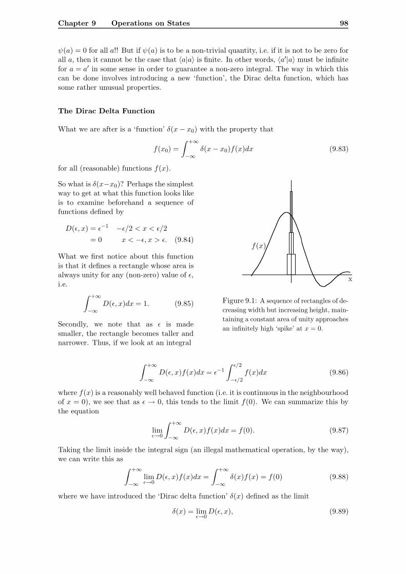
Chapter 9 Operations on States 98
ψ(a) = 0 for all a!! But if ψ(a) is to be a non-trivial quantity, i.e. if it is not to be zero forall a, then it cannot be the case that 〈a|a〉 is finite. In other words, 〈a′|a〉 must be infinitefor a = a′ in some sense in order to guarantee a non-zero integral. The way in which thiscan be done involves introducing a new ‘function’, the Dirac delta function, which hassome rather unusual properties.
The Dirac Delta Function
What we are after is a ‘function’ δ(x− x0) with the property that
f(x0) =∫ +∞
−∞δ(x− x0)f(x)dx (9.83)
for all (reasonable) functions f(x).
So what is δ(x−x0)? Perhaps the simplestway to get at what this function looks likeis to examine beforehand a sequence offunctions defined by
D(ε, x) = ε−1 −ε/2 < x < ε/2= 0 x < −ε, x > ε. (9.84)
What we first notice about this functionis that it defines a rectangle whose area isalways unity for any (non-zero) value of ε,i.e. ∫ +∞
−∞D(ε, x)dx = 1. (9.85)
Secondly, we note that as ε is madesmaller, the rectangle becomes taller andnarrower. Thus, if we look at an integral
f(x)
x
Figure 9.1: A sequence of rectangles of de-creasing width but increasing height, main-taining a constant area of unity approachesan infinitely high ‘spike’ at x = 0.
∫ +∞
−∞D(ε, x)f(x)dx= ε−1
∫ ε/2
−ε/2f(x)dx (9.86)
where f(x) is a reasonably well behaved function (i.e. it is continuous in the neighbourhoodof x = 0), we see that as ε → 0, this tends to the limit f(0). We can summarize this bythe equation
limε→0
∫ +∞
−∞D(ε, x)f(x)dx= f(0). (9.87)
Taking the limit inside the integral sign (an illegal mathematical operation, by the way),we can write this as∫ +∞
−∞limε→0
D(ε, x)f(x)dx =∫ +∞
−∞δ(x)f(x) = f(0) (9.88)
where we have introduced the ‘Dirac delta function’ δ(x) defined as the limit
δ(x) = limε→0
D(ε, x), (9.89)
Chapter 9 Operations on States 99
a function with the unusual property that it is zero everywhere except for x = 0, where itis infinite.
The above defined function D(ε, x) is but one ‘representation’ of the Dirac delta function.There are in effect an infinite number of different functions that in an appropriate limitbehave as the rectangular function here. Some examples are
δ(x− x0) = limL→∞
1π
sinL(x− x0)x− x0
= limε→0
1π
ε
(x− x0)2 + ε2(9.90)
= limλ→∞
λe−λ|x−x0|.
In all cases, the function on the right hand side becomes narrower and taller as the limitis taken, while the area under the various curves remains the same, that is, unity.
The delta function is not to be thought of as a function as it is usually defined in puremathematics, but rather it is to be understood that a limit of the kind outlined above isimplied whenever the delta function appears in an integral. However, such mathematicalniceties do not normally need to be a source of concern in most instances. It is usuallysufficient to be aware of the basic property Eq. (9.83) and a few other rules that can beproven using the limiting process, such as
δ(x) = δ(−x)∫ +∞
−∞δ(x− x0)δ(x− x1) = δ(x0 − x1)∫ +∞
−∞f(x)δ′(x− x0)dx = −f ′(x0).
The limiting process should be employed if there is some doubt about any result obtained.For instance, it can be shown that the square of a delta function cannot be given asatisfactory meaning.
Delta Function Normalization of Eigenstates
Returning to the result
ψ(a′) =∫ α2
α1
〈a′|a〉ψ(a)da (9.91)
we see that the inner product 〈a′|a〉, must be interpreted as a delta function:
〈a′|a〉 = δ(a− a′). (9.92)
The states |a〉 are said to be delta function normalized, in contrast to the orthonormalproperty of discrete eigenstates.
One result of this is that states such as |a〉 are of infinite norm and so cannot be normalizedto unity. Such states states cannot represent possible physical states of a system, thoughit is often convenient, with caution, to speak of such states as if they were physicallyrealizable. Mathematical (and physical) paradoxes can arise if care is not taken. However,linear combinations of these states can be normalized to unity, as this following exampleillustrates.
Chapter 9 Operations on States 100
If we consider a state |ψ〉 given by
|ψ〉 =∫ α2
α1
|a〉〈a|ψ〉da, (9.93)
then
〈ψ|ψ〉 =∫ α2
α1
〈ψ|a〉〈a|ψ〉da. (9.94)
But 〈a|ψ〉= ψ(a) and 〈ψ|a〉= ψ(a)∗, so that
〈ψ|ψ〉=∫ α2
α1
|ψ(a)|2da. (9.95)
Provided |ψ(a)|2 is a well behaved function, this integral will converge to a finite result,so that the state |ψ〉 can indeed be normalized to unity.
9.5 Dirac Notation for Operators
The above discussion of the properties of operators was based on making direct use ofthe defining properties of an operator, that is, in terms of their actions on ket vectors,in particular the vectors belonging to a set of basis states. All of these properties canbe represented in a very succinct way that makes explicit use of the Dirac notation. Theessential idea is to give a meaning to the symbol |φ〉〈ψ|. The interpretation that is givenis defined as follows: (
|φ〉〈ψ|)|α〉 = |φ〉〈ψ|α〉
〈α|(|φ〉〈ψ|
)= 〈α|φ〉〈ψ|
(9.96)
i.e. it maps kets into kets and bras into bras, exactly as an operator is supposed to.
If we further require |φ〉〈ψ| to have the linear property
|φ〉〈ψ|(c1|ψ1〉+ c2|ψ2〉
)= c1
(|φ〉〈ψ|
)|ψ1〉+ c2
(|φ〉〈ψ|
)|ψ2〉
= |φ〉(c1〈ψ|ψ1〉+ c2〈ψ|ψ2〉
)(9.97)
and similarly for the operator acting on bra vectors, we have given the symbol the prop-erties of a linear operator.
We can further generalize this to include sums of such bra-ket combinations, e.g.
c1|φ1〉〈ψ1|+ c2|φ2〉〈ψ2|
where c1 and c2 are complex numbers, is an operator such that(c1|φ1〉〈ψ1|+ c2|φ2〉〈ψ2|
)|ξ〉 = c1|φ1〉〈ψ1|ξ〉+ c2|φ2〉〈ψ2|ξ〉 (9.98)
and similarly for the action on bra vectors.
Below we describe a number of important properties and examples that illustrate theusefulness of this notation.
Chapter 9 Operations on States 101
Projection Operators In this notation, a projection operator P will be simply givenby
P = |ψ〉〈ψ| (9.99)
provided |ψ〉 is normalized to unity, since we have
P 2 = |ψ〉〈ψ|ψ〉〈ψ|= |ψ〉〈ψ|= P (9.100)
as required for a projection operator.
Completeness Relation This new notation also makes it possible to express the com-pleteness relation in a particularly compact form. Recall that if the set of ket vectors{|ϕn〉; n = 1, 2, 3 . . .} is a complete set of orthonormal basis states for the state space of asystem, then any state |ψ〉 can be written
|ψ〉 =∑n
|ϕn〉〈ϕn|ψ〉 (9.101)
which in our new notation can be written
|ψ〉 =(∑
n
|ϕn〉〈ϕn|)|ψ〉 (9.102)
so that we must conclude that ∑n
|ϕn〉〈ϕn| = 1 (9.103)
where 1 is the unit operator. We can see that the individual terms in the sum, that isthe |ϕn〉〈ϕn|, are just projection operators, so that we have shown that the competenessrelation can be expressed as a sum over a set of projection operators defined in terms ofthe basis states {|ϕn〉; n = 1, 2, 3 . . .}. It is often referred to as a decomposition of unity.
In the case of continuous eigenvalues, the same argument as above can be followed through.Thus, if we suppose that a Hermitean operator A has a set of eigenstates {|a〉;α1 < a <
α2}, then we can readily show that ∫ α2
α1
|a〉〈a|da = 1. (9.104)
Note that, in practice, it is often the case that an operator can have both discrete andcontinuous eigenvalues, in which case the completeness relation can be written∑
n
|ϕn〉〈ϕn|+∫ α2
α1
|a〉〈a|da = 1 (9.105)
The completeness relation experssed in this fashion (in both the discrete and continuouscases) is extremely important and has widespread use in calculational work, as illustratedin the following examples.
Example 9.8 Show that any operator can be expressed in terms of this Dirac notation.
We can see this for an operator A by writing
A = 1A 1 (9.106)
Chapter 9 Operations on States 102
and using the decomposition of unity twice over to give
A =∑m
∑n
|ϕm〉〈ϕm|A|ϕn〉〈ϕn|
=∑m
∑n
|ϕm〉〈ϕn|Amn (9.107)
where Amn = 〈ϕm|A|ϕn〉.
Example 9.9 Using the decomposition of unity in terms of the basis states {|ϕn〉; n =1, 2, 3 . . .}, expand A|ϕm〉 in terms of these basis states.
This calculation proceeds by inserting the unit operator in a convenient place:
A|ϕm〉 = 1A|ϕm〉 =(∑
n
|ϕn〉〈ϕn|)A|ϕm〉
=∑n
|ϕn〉〈ϕn|A|ϕm〉
=∑n
Anm|ϕn〉 (9.108)
where Anm = 〈ϕn|A|ϕm〉.
Example 9.10 Using the decomposition of unity, we can insert the unit operator betweenthe two operators in the quantity 〈ψ|AB|φ〉 to give
〈ψ|AB|φ〉 = 〈ψ|A 1B|φ〉 =∑n
〈ψ|A|ϕn〉〈ϕn|B|φ〉. (9.109)
Hermitean conjugate of an operator It is straightforward to write down the Her-mitean conjugate of an operator. Thus, for the operator A given by
A =∑n
cn|φn〉〈ψn| (9.110)
we have
〈φ|A|ψ〉 =∑n
cn〈φ|φn〉〈ψn|ψ〉 (9.111)
so that taking the complex conjugate we get
〈ψ|A†|φ〉 =∑n
c∗n〈ψ|ψn〉〈φn|φ〉 = 〈ψ|(∑
n
c∗n|ψn〉〈φn|)|φ〉. (9.112)
We can then extract from this the result
A† =∑n
c∗n|ψn〉〈φn|. (9.113)
Chapter 9 Operations on States 103
Spectral decomposition of an operator As a final important example, we can lookat the case of expressing an Hermitean operator in terms of projectors onto its basisstates. Thus, if we suppose that A has the eigenstates {|an〉; n = 1, 2, 3 . . .} and associatedeigenvalues an, n = 1, 2, 3 . . . , so that
A|an〉 = an|an〉 (9.114)
then by noting that the eigenstates of A form a complete orthonormal set of basis stateswe can write the decomposition of unity in terms of the eigenstates of A as∑
n
|an〉〈an| = 1. (9.115)
Thus we find that
A = A 1 = A∑n
|an〉〈an| =∑n
A|an〉〈an| =∑n
an|an〉〈an|. (9.116)
so that
A =∑n
an|an〉〈an|. (9.117)
The analogous result for continuous eigenstates is then
A =∫ α2
α1
a|a〉〈a|da (9.118)
while if the operator has both continuous and discrete eigenvalues, the result is
A =∑n
an|an〉〈an|+∫ α2
α1
a|a〉〈a|da. (9.119)
This is known as the spectral decomposition of the operator A, the name coming, in part,from the fact that the collection of eigenvalues of an operator is known as its eigenvaluespectrum.
Chapter 10
Representations of State Vectorsand Operators
In the preceding Chapters, the mathematical ideas underpinning the quantum theory havebeen developed in a fairly general (though, admittedly, not a mathematically rigorous)fashion. However, much that has been presented, particularly the concept of an operator,can be developed in another way that is, in some respects, less abstract than what has beenused so far. This alternate form of presentation involves working with the componentsof the state vectors and operators, leading to their being represented by column androw vectors, and matrices. This development of the theory is completely analogous tothe way in which this is done when dealing with the position vector in ordinary threedimensional space. Below, we will look at how the idea of writing the position vectors intwo dimensional space can be written in terms of column and row vectors. We will thenuse the ideas developed there to show how state vectors and operators can be expressed ina similar fashion. This alternate route offers another way of introducing such concepts asadding, multiplying and taking the inverse of operators through their representations asmatrices, and further provides another way to introduce the idea of the Hermitean adjointof an operator, and of a Hermitian operator.
10.1 Representation of Vectors as Column and Row Vectors
When writing down a vector, we have so far made explicit the basis vectors when writingan expression such as r = xi+ yj for a position vector, or |S〉 = a|+〉+ b|−〉 for the stateof a spin half system. But the choice of basis vectors is not unique, i.e. we could use anyother pair of orthonormal unit vectors i′ and j′, and express the vector r in terms of thesenew basis vectors, though of course the components of r will change. The same is true forthe spin basis vectors |±〉, i.e. we can express the state |S〉 in terms of some other basisvectors, with, though once again, the components of |S〉 will now be different. But it istypically the case that once the choice of basis vectors have been decided on, it should notbe necessary to always write them down when writing down a vector, i.e. it would be justas useful to just write down the components of a vector. Doing this leads to a convenientnotation in which vectors are written in terms of column and row vectors. It also providesa direct route to some of the important mathematical entities encountered in quantummechanics such as bra vectors and operators that are more rigorously introduced in a moreabstract way.
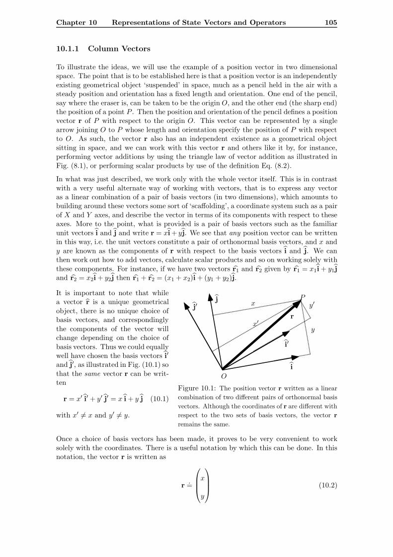
Chapter 10 Representations of State Vectors and Operators 105
10.1.1 Column Vectors
To illustrate the ideas, we will use the example of a position vector in two dimensionalspace. The point that is to be established here is that a position vector is an independentlyexisting geometrical object ‘suspended’ in space, much as a pencil held in the air with asteady position and orientation has a fixed length and orientation. One end of the pencil,say where the eraser is, can be taken to be the origin O, and the other end (the sharp end)the position of a point P . Then the position and orientation of the pencil defines a positionvector r of P with respect to the origin O. This vector can be represented by a singlearrow joining O to P whose length and orientation specify the position of P with respectto O. As such, the vector r also has an independent existence as a geometrical objectsitting in space, and we can work with this vector r and others like it by, for instance,performing vector additions by using the triangle law of vector addition as illustrated inFig. (8.1), or performing scalar products by use of the definition Eq. (8.2).
In what was just described, we work only with the whole vector itself. This is in contrastwith a very useful alternate way of working with vectors, that is to express any vectoras a linear combination of a pair of basis vectors (in two dimensions), which amounts tobuilding around these vectors some sort of ‘scaffolding’, a coordinate system such as a pairof X and Y axes, and describe the vector in terms of its components with respect to theseaxes. More to the point, what is provided is a pair of basis vectors such as the familiarunit vectors i and j and write r = xi+ yj. We see that any position vector can be writtenin this way, i.e. the unit vectors constitute a pair of orthonormal basis vectors, and x andy are known as the components of r with respect to the basis vectors i and j. We canthen work out how to add vectors, calculate scalar products and so on working solely withthese components. For instance, if we have two vectors r1 and r2 given by r1 = x1i+ y1jand r2 = x2i+ y2j then r1 + r2 = (x1 + x2)i+ (y1 + y2)j.
It is important to note that whilea vector r is a unique geometricalobject, there is no unique choice ofbasis vectors, and correspondinglythe components of the vector willchange depending on the choice ofbasis vectors. Thus we could equallywell have chosen the basis vectors i′
and j′, as illustrated in Fig. (10.1) sothat the same vector r can be writ-ten
r = x′ i′ + y′ j′ = x i+ y j (10.1)
with x′ �= x and y′ �= y.
i
i′
jj′
r
y
x y′
x′
P
O
Figure 10.1: The position vector r written as a linearcombination of two different pairs of orthonormal basisvectors. Although the coordinates of r are different withrespect to the two sets of basis vectors, the vector rremains the same.
Once a choice of basis vectors has been made, it proves to be very convenient to worksolely with the coordinates. There is a useful notation by which this can be done. In thisnotation, the vector r is written as
r .=
xy
(10.2)
Chapter 10 Representations of State Vectors and Operators 106
what is known as a column vector. We then say that this column vector is a representationof the vector r with respect to the basis vectors i and j.
It is important to note that we do not say that r equals the column vector, in fact it is notan equal sign that is used in Eq. (10.2), rather the symbol ‘ .=’ is used, which is to be readas ‘is represented by’. The reason for this is that, as mentioned above, while the vectorr is a unique geometrical object, its components are not – they depend on the choice ofbasis vectors. We could have equally chosen basis vectors i′ and j′, and hencesince thecomponents x′ and y′ will be, in general, different from x and y, we end up with a differentcolumn vector representing the same vector:
r .=
x′y′
. (10.3)
i.e. two apparently different column vectors representing the same vector r. Equivalently,if we had two column vectors with exactly the same numbers in the two positions, wecould not conclude that they represent the same vector unless we were told that the basisvectors were the same in each case. Thus if there is any chance of ambiguity, we needto make it clear when we use the column vector notation, exactly what the basis vectorsare. The terminology then is to say that the vector r is given by the column vector inEq. (10.2) in the {i, j} representation.
Once a choice of basis vectors has been settled on, and consistently used, we can proceedwith vector calculations using the new notation. Thus, for instance, we can add twovectors:
r = r1 + r2 (10.4)
which becomes, using the {i, j} representationxy
=
x1
y1
+
x2
y2
=
x1 + x2
y1 + y2
. (10.5)
10.1.2 Row Vectors
The scalar product (r1, r2) = r1 · r2 can be calculated by using the usual rule r1 · r2 =r1r2 cos θ, but it can also be expressed in terms of the components of r1 and r2 in, say, the{i, j} representation, though note that the same numerical result is obtained whaateverrepresentation is used. The result is simply
(r1, r2) = r1 · r2 = x1x2 + y1y2. (10.6)
At this point we note that, if we use the rules of matrix multiplication, this last result canbe written
(r1, r2) = r1 · r2 =(x1 y1
)x2
y2
(10.7)
Chapter 10 Representations of State Vectors and Operators 107
where we note the appearance of the column vector representing the vector r2, but r1, thefirst factor in the scalar product, has been represented by a row vector. If the componentsof r1 and r2 were complex, then we would write the inner product as
(r1, r2) = r∗1 · r2 = x∗1x2 + y∗1y2 =(x∗1 y∗1
)x2
y2
(10.8)
The use of a row vector to represent r1 can be looked on here as a convenience so that therules of matrix multiplication can be applied, but there is a deeper significance to its use1
that will become apparent when we look at the column and row vector representations ofket and bra vectors.
10.1.3 Probability Amplitudes, Inner Products and Bra Vectors
We saw above that the expression
|S〉 = |−〉〈−|S〉+ |+〉〈+|S〉
can be interpreted as the state |S〉 being expressed as a linear combination of the twobasis states |±〉. We further saw that quantities such as 〈+|+〉, 〈+|−〉 and so on can beput into direct correspondence with the inner products of (complex) unit vectors, so thatthese basis states |±〉 are orthonormal. We can complete the analogy with the case ofordinary vectors by noting that we could then write this ket vector as a column vector,i.e.
|S〉 .=
〈−|S〉〈+|S〉
. (10.9)
If we pursue this line further, we can get an idea of how to interpret bra vectors. To dothis, consider the more general probability amplitudes 〈S ′|S〉. This we can write as
〈S ′|S〉 = 〈S ′|−〉〈−|S〉+ 〈S ′|+〉〈+|S〉. (10.10)
If we now use
〈±|S〉 = 〈S|±〉∗ (10.11)
this becomes
〈S ′|S〉 = 〈−|S ′〉∗〈−|S〉+ 〈+|S ′〉∗〈+|S〉 (10.12)
which we can write as
〈S ′|S〉 =(〈−|S ′〉∗ 〈+|S ′〉∗
)〈−|S〉〈+|S〉
. (10.13)
1Effectively, what is going on is that corresponding to any vector r represented by a column vector,there corresponds another vector r∗ known as its dual which is represented by a row vector. The originalvector is the ‘physical’ vector while its dual is an abstract mathematical companion. The original vectorand its dual belong to two different vector spaces.
Chapter 10 Representations of State Vectors and Operators 108
In other words, the bra vector 〈S ′| is represented by the row vector
〈S ′| .=(〈−|S ′〉∗ 〈+|S ′〉∗
). (10.14)
This shows that a bra vector is more than just the ‘complex conjugate’ of a ket vector,since a row vector is not the same as a column vector.
10.2 Representations of State Vectors and Operators
The procedure here is identical to that which was followed in the case of the positionvector, i.e. we introduce a complete set of orthonormal basis states {|ϕn〉; n = 1, 2, . . .}that span the state space of the quantum system, and then work with the components ofthe ket and bra vectors, and the operators. Of course, we now do not have the luxury ofinterpreting these basis vectors as representing physical directions in real space – ratherthey are abstract vectors in a multi-dimensional complex vector space, but much of whathas been said above in connection with vectors in ordinary space can be carried over tothis more abstract situation.
10.2.1 Representation of Ket and Bra Vectors
In terms of the basis states {|ϕn〉; n = 1, 2, . . .}, an arbitrary state vector |ψ〉 can bewritten as
|ψ〉 =∑n
|ϕn〉〈ϕn|ψ〉. (10.15)
Let us now write
〈ϕn|ψ〉 = ψn. (10.16)
We then have, by analogy with the position vector:
|ψ〉 .=
ψ1
ψ2
ψ3
...
. (10.17)
This is a representation of |ψ〉 as a column vector with respect to the set of basis states{|ϕn〉; n = 1, 2, . . .}. In particular, the basis state |ϕm〉 will have components
(ϕm)n = 〈ϕn|ϕm〉 = δnm (10.18)
and so they will be represented by column vectors of the form
|ϕ1〉.=
1
0
0
...
|ϕ2〉
.=
0
1
0
...
. . . (10.19)
Chapter 10 Representations of State Vectors and Operators 109
i.e. the mth component ϕnm of |ϕn〉 is zero except in the mth position where ϕmm = 1.
Now form the inner product 〈χ|ψ〉:
〈χ|ψ〉 =∑n
〈χ|ϕn〉〈ϕn|ψ〉. (10.20)
We know that 〈χ|ϕn〉 = (〈ϕn|χ〉)∗, and following on from the notation introduce above,we write χn = 〈ϕn|χ〉 so that
〈χ|ϕn〉 = χ∗n (10.21)
and hence
〈χ|ψ〉 =∑n
χ∗nψn (10.22)
which we can write as
〈χ|ψ〉 =(χ∗1 χ∗2 χ∗3 . . .
)
ψ1
ψ2
ψ3
...
(10.23)
which we evaluate by the usual rules of matrix multiplication. Note that here we havemade the identification of the bra vector 〈χ| as a row vector:
〈χ| .=(χ∗1 χ∗2 χ∗3 . . .
)(10.24)
with respect to the set of basis states {|ϕn〉; n = 1, 2, . . .}. This can be compared with therepresentation of the ket vector |χ〉 as a column vector:
|χ〉 .=
χ∗1
χ∗2
χ∗3
...
. (10.25)
This difference in appearance of the representation of a bra and a ket vector, the firstas a row vector, the second as a column vector, perhaps emphasizes the point made inSection 8.4.2 that the bra vectors form a vector space, the dual Hilbert space H∗ relatedto, but distinct from, the Hilbert space H of the ket vectors. In a sense, a bra vector canbe thought of as something akin to being the ‘complex conjugate’ of its corresponding ketvector.
Chapter 10 Representations of State Vectors and Operators 110
10.2.2 Representation of Operators
Now turn to the operator equation
A|ψ〉 = |φ〉 (10.26)
which we can write as
|φ〉 = A|ψ〉 = A∑n
|ϕn〉〈ϕn|ψ〉 =∑n
A|ϕn〉〈ϕn|ψ〉. (10.27)
Then
〈ϕm|φ〉 =∑n
〈ϕm|A|ϕn〉〈ϕn|ψ〉 (10.28)
which we can write as
φm =∑n
Amnψn (10.29)
where
Amn = 〈ϕm|A|ϕn〉. (10.30)
We can write this as a matrix equation:
φ1
φ2
φ3
...
=
A11 A12 A13 . . .
A21 A22 A23 . . .
A31 A32 A33 . . .
......
...
ψ1
ψ2
ψ3
...
(10.31)
where the operator A is represented by a matrix :
A.=
A11 A12 A13 . . .
A21 A22 A23 . . .
A31 A32 A33 . . .
......
...
. (10.32)
The quantities Amn are known as the matrix elements of the operator A with respect tothe basis states {|ϕn〉; n = 1, 2, . . .}.
It is important to keep in mind that the column vectors, row vectors, and matrices aboveare constructed with respect to a particular set of basis states. If a different set of basisstates are used, then the state vectors and operators remain the same, but the column orrow vector, or matrix representing the state vector or operator respectively will change.Thus, to give any meaning to a row vector, or a column vector, or a matrix, it is essential
Chapter 10 Representations of State Vectors and Operators 111
that the basis states be known. An important part of quantum mechancis is the math-ematical formalism that deals with transforming between different sets of basis states.However, we will not be looking at transformation theory here.
Example 10.1 Consider two state vectors
|1〉 = 1√2
[|−〉 − i|+〉
]|2〉 = 1√
2
[|−〉+ i|+〉
]where |±〉 are the usual base states for a spin half system. We want to represent theseket vectors as column vectors with respect to the set of basis states {|+〉, |−〉}. Firstly, wecan write
|+〉 .=
1
0
and |−〉 .=
0
1
.
We can then express the states |1〉 and |2〉 in column vector notation as
|1〉 .= 1√2
−i1
which can also be written as
|1〉 .= − i√2
1
0
+ 1√2
0
1
.
The corresponding bra vectors are
〈1| = 1√2
[〈−|+ i〈+|
]〈2| = 1√
2
[〈−| − i〈+|
]or, as row vectors
〈1| .=(i 1
)and 〈2| .=
(−i 1
).
We can calculate inner products as follows:
〈1|2〉 = 12
(i 1
)i1
= 0,
〈1|1〉 = 12
(i 1
)−i1
= 1.
and so on.
Chapter 10 Representations of State Vectors and Operators 112
Example 10.2 We can also look at the operator A defined by
A|±〉 = ±12 i�|∓〉
which can be written out in matrix form as
A.=
〈+|A|+〉 〈+|A|−〉〈−|A|+〉 〈−|A|−〉
=
0 −12 i�
12i� 0
so that, for instance
A|1〉 .=
0 −12 i�
12 i� 0
− i√
2
1√2
= −12 i�
1√2
i√2
= 12�
− i√2
1√2
.
Thus we have A|1〉 = 12�|1〉, which incidentally shows that |1〉 is an eigenstate of A.
Using the representations of bra vectors and operators, it is straightforward to see whatthe action of an operator on a bra vector is given by. Thus, we have:
〈ψ|A .=(ψ1 ψ2 ψ3 . . .
)
A11 A12 A13 . . .
A21 A22 A23 . . .
A31 A32 A33 . . .
......
...
=(ψ1A11 + ψ2A21 + . . . ψ2A12 + ψ2A22 + . . . ψ1A13 + ψ2A23 + . . . . . .
). (10.33)
The final result can then be written in the corresponding bra vector notation if desired.This can be illustrated by example.
Example 10.3 Evaluate 〈2|A using the representations of the bra vector |2〉 and operatorA:
〈2|A .= 1√2
(−i 1
)0− 12i�
12 i�
=
1√2
(12i� −1
2�
)= −1
2� · 1√2
(−i 1
)
Chapter 10 Representations of State Vectors and Operators 113
which can be written as 〈2|A = −12�〈2|.
10.2.3 Properties of Matrix Representations of Operators
Many of the properties of operators can be expressed in terms of the properties of theirrepresentative matrices. Most of these properties are straightforward, and will be presentedbelow without comment.
Equality
Two operators are equal if their corresponding operator matrix elements are equal, i.e. A =B if Amn = Bmn.
Unit and Zero Operator
The unit operator 1 is the operator such that 1|ψ〉 = |ψ〉 for all states |ψ〉. It has thethe matrix elements 1mn = δmn, i.e. the diagonal elements are all unity, and the off-diagonal elements are all zero. The unit operator has the same form in all representations,i.e. irrespective of the choice of basis states.
The zero operator 0 is the operator such that 0|ψ〉 = 0 for all states |ψ〉. Its matrixelements are all zero.
Addition of Operators
Given two operators A and B with matrix elements Amn and Bmn, then the matrixelements of their sum S = A+ B are given by
Smn = Amn +Bmn. (10.34)
Multiplication by a Complex Number
If λ is a complex number, then the matrix elements of the operator C = λA are given by
Cmn = λAmn. (10.35)
Product of Operators
Given two operators A and B with matrix elements Amn and Bmn, then the matrixelements of their product P = AB are given by
Pmn =∑k
AmkBkn (10.36)
i.e. the usual rule for the multiplication of two matrices.
Matrix multiplication, and hence operator multiplication, is not commutative, i.e. in gen-eral AB �= BA. The difference, AB − BA, known as the commutator of A and B andwritten [A, B], can be readily evaluated using the matrix representations of A and B.
Chapter 10 Representations of State Vectors and Operators 114
Example 10.4 Three operators σ1, σ2 and σ3, known as the Pauli spin matrices, thatoccur in the theory of spin half systems (and elsewhere) have the matrix representationswith respect to the {|+〉, |−〉} basis given by
σ1.=
0 1
1 0
σ2.=
0 −i
i 0
σ3.=
1 0
0 −1
.
The commutator [σ1, σ2] can be readily evaluated using these matrices:
[σ1, σ2] = σ1σ2 − σ2σ1
.=
0 1
1 0
0 −i
i 0
−0 −i
i 0
0 1
1 0
=
i 0
0 −i
−−i 0
0 i
= 2i
1 0
0 −1
The final matrix can be recognized as the representation of σ3, so that overall we haveshown that
[σ1, σ2] = 2iσ3.
Cyclic permutation of the subscripts then gives the other two commutators.
Functions of Operators
If we have a function f(x) which we can expand as a power series in x:
f(x) = a0 + a1x+ a2x2 + · · · =
∞∑n=0
anxn (10.37)
then we define f(A), a function of the operator A, to be also given by the same powerseries, i.e.
f(A) = a0 + a1A+ a2A2 + · · · =
∞∑n=0
anAn. (10.38)
Once again, using the matrix representation of A, it is possible, in certain cases, to workout what the matrix representation is of f(A).
Example 10.5 One of the most important functions of an operator that is encounteredis the exponential function. To illustrate what this means, we will evaluate here the
Chapter 10 Representations of State Vectors and Operators 115
exponential function exp(iφσ3) where σ1 is one of the Pauli spin matrices introducedabove, for which
σ1.=
0 1
1 0
and φ is a real number. Using the power series expansion of the exponential function, wehave
eiφbσ1 =∞∑n=0
iφn
n!σn1 .
It is useful to note that
σ23.=
0 1
1 0
2
=
1 0
0 1
i.e. σ2
1 = 1, the identity operator. Thus we can always write
σ2n1 = 1 σ2n+1
1 = σ3.
Thus, if we separate the infinite sum into two parts:
eiφbσ1 =∞∑n=0
(iφ)2n
(2n)!σ2n
1 +∞∑n=0
(iφ)2n+1
(2n+ 1)!σ2n+1
1
where the first sum is over all the even integers, and the second over all the odd integers,we get
eiφbσ1 = 1∞∑n=0
(−1)nφ2n
(2n)!+ iσ1
∞∑n=0
(−1)nφ2n+1
(2n+ 1)!
= cosφ+ iσ1 sinφ
.=
cosφ 0
0 cosφ
+
0 i sinφ
i sinφ 0
=
cosφ i sinφ
i sinφ cosφ
.
Inverse of an Operator
Finding the inverse of an operator, given its matrix representation, amounts to finding theinverse of the matrix, provided, of course, that the matrix has an inverse.
Chapter 10 Representations of State Vectors and Operators 116
Example 10.6 The inverse of exp(iφσ1) can be found by taking the inverse of its repre-sentative matrix:
(eiφbσ1
)−1 .=
cosφ i sinφ
i sinφ cosφ
−1
=
cosφ −i sinφ
−i sinφ cosφ
.
This inverse can be recognized as being just cosφ −i sinφ
−i sinφ cosφ
=
cos(−φ) i sin(−φ)
i sin(−φ) cos(−φ)
which means that (
eiφbσ1)−1 = e−iφbσ1
a perhaps unsurprising result in that it is a particular case of the fact that the inverse ofexp(A) is just exp(−A), exactly as is the case for the exponential function of a complexvariable.
10.2.4 Eigenvectors and Eigenvalues
Operators act on states to map them into other states. Amongst the possible outcomesof the action of an operator on a state is to map the state into a multiple of itself:
A|φ〉 = aφ|φ〉 (10.39)
where |φ〉 is, in general, a complex number. The state |φ〉 is then said to be an eigenstateor eigenket of the operator A with aφ the associated eigenvalue.
The fact that operators can possess eigenstates might be thought of as a mathematical factincidental to the physical content of quantum mechanics, but it turns out that the oppositeis the case: the eigenstates and eigenvalues of various kinds of operators are essentialparts of the physical interpretation of the quantum theory, and hence warrant close study.Notationally, is is often useful to use the eigenvalue assocaited with an eigenstate to labelthe eigenvector, i.e. notation
A|a〉 = a|a〉. (10.40)
This notation, or minor variations of it, will be used almost exclusively here.
Determining the eigenvalues and eigenvectors of a given operator A, occasionally referredto as solving the eigenvalue problem for the operator, amounts to finding solutions to theeigenvalue equation A|φ〉 = aφ|φ〉. Written out in terms of the matrix representations ofthe operator with respect to some set of orthonormal basis vectors {|ϕ〉; n = 1, 2, . . .}, thiseigenvalue equation is
A11 A12 . . .
A21 A22 . . .
......
φ1
φ2
...
= a
φ1
φ2
...
. (10.41)
Chapter 10 Representations of State Vectors and Operators 117
This expression is equivalent to a set of simultaneous, homogeneous, linear equations:A11 − a A12 . . .
A21 A22 − a . . .
......
φ1
φ2
...
= 0 (10.42)
which have to be solved for the possible values for a, and the associated values for thecomponents φ1, φ2, . . . of the eigenvectors. The procedure is standard. The determinantof coefficients must vanish in order to get non-trivial solutions for the components φ1, φ2,. . . : ∣∣∣∣∣∣∣∣∣∣∣∣
A11 − a A12 . . .
A21 A22 − a . . .
......
∣∣∣∣∣∣∣∣∣∣∣∣= 0 (10.43)
which yields an equation known as the secular equation, or characteristic equation, thathas to be solved to give the possible values of the eigenvalues a. Once these are known,they have to be resubstituted into Eq. (10.41) and the components φ1, φ2, . . . of theassociated eigenvectors determined. The details of how this is done properly belongs toa text on linear algebra and will not be considered any further here, except to say thatthe eigenvectors are typically determined up to an unknown multiplicative constant. Thisconstant is usually fixed by the requirement that these eigenvectors be normalized to unity.In the case of repeated eigenvalues, i.e. when the characteristic polynomial has multipleroots (otherwise known as degenerate eigenvalues), the determination of the eigenvectorsis made more complicated still. Once again, issues connected with these kinds of situationswill not be considered here.
In general, it is found that the above eigenvalue problem shows that the operator A mayhave
1. no eigenstates;
2. a discrete collection of eigenvalues a1, a2, . . . and associated eigenvectors |a1〉, |a2〉,. . . ;
The collection of all the eigenvalues of an operator is called the eigenvalue spectrum of theoperator. Note also that more than one eigenvector can have the same eigenvalue. Suchan eigenvalue is said to be degenerate.
For the present we will be confining our attention to to operators that have discrete eigen-value spectra. Modifications needed to handle continuous eigenvalues will be introducedlater.
10.2.5 Hermitean Operators
Apart from certain calculational advantages, the representation of operators as matricesmakes it possible to introduce in a direct fashion Hermitean operators, already considered
Chapter 10 Representations of State Vectors and Operators 118
in a more abstract way in Section 9.3.1, which have a central role to play in the physicalinterpretation of quantum mechanics.
To begin with, suppose we have an operator A with matrix elements Amn with respect toa set of orthonormal basis states {|ϕn〉; n = 1, 2, . . .}. From the matrix representing thisoperator, we can construct a new operator by taking the transpose and complex conjugateof the original matrix:
A11 A12 A13 . . .
A21 A22 A23 . . .
A31 A32 A33 . . .
......
...
−→
A∗11 A∗
21 A∗31 . . .
A∗12 A∗
22 A∗32 . . .
A∗13 A∗
23 A∗33 . . .
......
...
. (10.44)
The new matrix will represent a new operator which is obviously related to A, which wewill call A†, i.e.
A† .=
(A†)11 (A†)12 (A†)13 . . .
(A†)21 (A†)22 (A†)23 . . .
(A†)31 (A†)32 (A†)33 . . .
......
...
=
A∗11 A∗
21 A∗31 . . .
A∗12 A∗
22 A∗32 . . .
A∗13 A∗
23 A∗33 . . .
......
...
. (10.45)
i.e.
〈ϕm|A†|ϕn〉 = (〈ϕn|A|ϕm〉)∗. (10.46)
The new operator that we have created, A† can be recognized as the Hermitean adjointof A. THe Hermitean adjoint has a useful property which we can most readily see if weuse the matrix representation of the operator equation
A|ψ〉 = |φ〉 (10.47)
which we earlier showed could be written as
φm =∑n
〈ϕm|A|ϕn〉ψn. (10.48)
If we now take the complex conjugate of this expression we find
φ∗m =∑n
ψ∗n〈ϕn|A†|ϕm〉 (10.49)
which we can write in row vector form as
(φ∗1 φ∗2 . . .
)=(ψ∗
1 ψ∗2 . . .
)
(A†)11 (A†)12 . . .
(A†)21 (A†)22 . . .
......
(10.50)
Chapter 10 Representations of State Vectors and Operators 119
which is the matrix version of
〈φ| = 〈ψ|A†. (10.51)
In other words we have shown that if A|ψ〉 = |φ〉, then 〈ψ|A† = 〈φ|, a result that we usedearlier to motivate the definition of the Hermitean adjoint in the first place. Thus, thereare two ways to approach this concept: either through a general abstract argument, or interms of matrix representations of an operator.
Example 10.7 Consider the operator A which has the representation in some basis
A.=
1 i
0 −1
.
Then
A† .=
1 0
−i −1
.
To be noticed in this example is that A �= A†.
Example 10.8 Now consider the operator
A.=
0 −i
i 0
.
Then
A† .=
0 −i
i 0
i.e. A = A†. THis is an example of a situation in which A and A† are identical. In thiscase, the operator is said to be selfadjoint, or Hermitean. Once again, we encounteredthis idea in a more general context in the previous Chapter, where it was remarked thatHermitean operators have a number of very important properties which leads to theirplaying a central role in the physical interpretation of quantum mechanics. There it wasshown that Hermitean operators have three properties:
1. The eigenvalues of a Hermitean operator are all real.
2. The eigenstates of a Hermitean operator belonging to different
Chapter 11
The Basic Postulates of QuantumMechanics
The material presented so far has been a mixtureof physics and mathematics, with thephysics motivating the mathematics, and the mathematics leading to new insights into thephysics. Sometimes explicitly, and sometimes implicitly, various rules have been used togive physical meaning to the mathematics – the Born interpretation of the wave functionis one example of an explicitly introduced rule of interpretation. But there are implicit inwhat has been said, ways of interpreting the mathematics that needs to be made explicit.For example we have frequently referred to the basis states | ± 1
2�〉 of a spin half particle,with the states labelled by the information we have obtained about the particle when ameasurement is made (using a Stern-Gerlach device in this case). This can be tied in withthe properties of a Hermitean operator in a way that introduces the idea of an observableinto quantum mechanics. The result is a set of rules, the basic postulates of quantummechanics which give us the ‘rules of the game’.
11.1 Quantum States are Vectors in a Hilbert Space
We begin with a restatement of the idea of state that we have dealt with before, that is, astate is as complete a description of the physical information that can be obtained abouta physical system as is possible without mutual interference or contradiction. The ideathen is that quantum states are as much states of knowledge as they are physical states.
The physical fact that a system can behave as if it is simultaneously in a number ofdifferent states, with the different possibilities revealing themselves in a purely randomfashion, then leads to the notion that this collection of information is to be considered avector which represents the state, and linear combinations of such vectors represents thisschizophrenic character of physical systems. The collection of vectors forms a complexHilbert space, known as the state space of the system. The first postulate then reads:
Postulate 1
Every state of a physical system is represented by a vector, and conversely, eachlinear superposition of vectors is representative of a possible state of the system. Ifa state of the system is represented by a vector |ψ〉, then the same state is representedby the vector c|ψ〉 where c is any non-zero complex number. The set of all statevectors describing a given physical system forms a complex vector space (or Hilbertspace) also known as the state space for the system. Only those states which canbe normalized to unity can represent physically realizable states.
Chapter 11 The Basic Postulates of Quantum Mechanics 121
There is one issue that is worthwhile considering here concerning the definition of a state interms of the information that is known about a system. What guarantee do we have that ifwe take an arbitrary linear combination of states for which we have complete information,that we create a state that also contains complete information about the system, and ifso, what is this complete information that the state contains? A definite answer cannot begiven to this question at this point, but we can get an idea that we can combine states tocreate states containing definite information by considering the case of spin half. We knowthat a spin half system can be prepared in either of the states |±〉, representing states inwhich the z component of the spin has the values ±1
2�, and that we cannot obtain anyfurther information about the spin half system without scrambling this information aboutthe z component. But if we form an arbitrary linear combination of |±〉, what physicalinformation on the spin of the particle is contained in the state so created?
To answer this question, we can make use of a result that can be obtained by a closerexamination of the behaviour of spin half atoms passing through Stern-Gerlach devices,which is that an arbitrary state can be written in the form
|Sn = 12�〉〉 = cos( 1
2θ)|+〉+ eiφ sin( 12θ)|−〉 (11.1)
where Sn = S · n, and where n = sin θ cosφ i+sin θ sinφ j+cos θ k is a unit vector orientedin a direction defined by the spherical polar angles θ, φ. This state is the state of a spinhalf particle that has emerged from a Stern-Gerlach apparatus in ‘spin up’ direction, where‘up’ is in the direction n of the magnetic field of the device.
Armed with this information, we are then able to take any linear combination of the states|±〉 and calculate from the coefficients what the angles θ and φ are, and hence the directionof n. For instance, if the system is in the state
|ψ〉 =1√2
(|+〉+ i|−〉
)(11.2)
then we know that cos 12θ = sin 1
2θ = 1/√
2 so that θ = π/2, and exp(iφ) = i so thatφ = π/2. Thus n points in the j direction, so that the state |ψ〉 = |Sy = 1
2�〉, i.e. theparticle is in a state for which the y component of spin has the value 1
2�, which is therequired physical information on the system contained in the state vector |ψ〉.
In more general situations, it is not at all an easy task to identify the information containedwithin an arbitrary state, at least in terms of the familiar properties that the system mightpossess, and as a general rule, it is not usually of much value to try to determine thisinformation. Nevertheless, it remains true that each state of a system contains definitephysical information of some properties of the system.
11.2 Observables of a Quantum System
The next postulate introduces the idea of an observable in quantum mechanics. As thename implies, an observable is a physical property of a quantum system that can bemeasured, and includes familiar physical properties such as position, momentum, angularmomentum and energy, and not so familiar properties as, for instance, photon number.The idea behind the concept has its seeds in what has been said before in the examplesgiven of how the basis states for the state space of a system is set up, and can, in part, beunderstood in terms of the idea that a state vector is specified by the information that isknown about a system.
Chapter 11 The Basic Postulates of Quantum Mechanics 122
Consider the example of, say, the molecular oxygen ion O−2 wherein the electron can reside
on either oxygen atom positioned at positions x = ±a. What this means is that if we wereto measure the position of the electron, we could get either of the results x = ±a and noother (within the limits of this simple model), and if we were to get the result x = a say,then we say that the system (the molecular oxygen ion) is then in the state |x = a〉, ormore simply just |a〉 where we have specified the state to the extent that we are able i.e. bylisting all the information that we have on the system. We therefore have a link betweenthe result x = a for the measurement of the position of the electron, and the state |a〉 thatwe then assign to the system. A similar statement can be made for the result x = −a andthe state |−a〉. We therefore have established a link between the states |±a〉 and the realnumbers ±a, the possible outcomes of the measurement of the position of the electron.
It is at this point that we recognize that the mathematics of vector spaces already providesus with a mathematical object that pairs off real numbers and state vectors, that is,Hermitean operators whose eigenvalues are real numbers. So, we construct out of theinformation we have on the position of the electron in the above example, a Hermiteanoperator which has as its eigenvalues ±a, and associated eigenstates |±a〉. As this operatorcontains information on the position of the electron in the molecule, we call this operatorthe position operator and represent it by the symbol x. The operator itself is known asan observable. In terms of the Dirac notation for an operator, we can then write
x = a|a〉〈a| − a| − a〉〈−a|. (11.3)
By this example, we see that an observable in quantum mechanics embodies all the possibleresults of a measurement of the observable, in contrast to the idea of a physical variablein classical physics which can only have one value (which we can, in principle, measureexactly).
Of course, it is generally the case that a particle can be found in a continuous range of po-sitions −∞ < x <∞, so that the position operator is x is then a Hermitean operator witha continuous range of eigenvalues. Consequently, the eigenstates of x are not normalizableto unity. We have instead
〈x|x′〉 = δ(x− x′) (11.4)
and the spectral decomposition of the operator is
x =∫ +∞
−∞x|x〉〈x|dx. (11.5)
The same argument can be applied to construct operators representing other observablequantities of a physical system, whether they be the energy, momentum, angular mo-mentum, photon number, and so on, which leads us to the general statement of thisfundamental postulate of quantum mechanics:
Postulate 2
To each physically measurable property (called an “observable”) of a physical sys-tem there corresponds a Hermitean operator (also called an “observable”) whoseeigenvalues are the possible results of measurements of the correspondi ng observ-able. Conversely, any Hermitean operator is understood as representing a possiblemeasureable property of the system.
It should be noted that not all observables are necessarily constructed in the fashion out-lined above. The analysis of the properties of quantum mechanical systems can lead us to
Chapter 11 The Basic Postulates of Quantum Mechanics 123
introduce new Hermitean operators whose physical interpretation needs to be determined.For instance, the energy observable (the Hamiltonian) and the momentum observable canbe shown to arise from arguments based on how we would expect quantum systems shouldbehave when displaced in time and space. In fact, it can be argued that all we need todo is define the position observable, and by symmetry arguments alone derive the otherobservables.
11.3 Completeness of Eigenstates of an Observable
The following postulate is also motivated by physical considerations, that is to say, theeigenvalues of an observable represent all the possible values for the associated observablephysical quantity:
Postulate 3
The eigenvectors of each observable associated with a physical system are assumedto form a complete set so that any state of the system can be expressed as a linearsuperposition of the eigenvectors of any observable of the system.
The associated eigenstates must be complete in the sense that any state of the systemmust have a component in the direction of at least one of the eigenstates of an observablefor the system. If it did not, this would mean that the system could somehow be preparedin a state for which there was zero probability of observing the system to have any valueof the observable, which is physically nonsensical. It is like saying that an electron couldbe prepared in a state in which there was no chance that a measurement of, say, its energy,will give any result at all.
Mathematically, this amounts to saying that if there is an observable A associated with acertain system, and the observable has the eigenstates {|an〉; n = 1, 2, 3 . . .} and associatedeigenvalues an; n = 1, 2, 3 . . . , and if the system is prepared in the state |ψ〉, then at leastone of the probability amplitudes 〈an|ψ〉 must be non-zero. If the dimension of the statespace is finite, then it can be proved that the eigenstates form a complete set, but thisis not the case if the state space has infinte dimension – it is assumed to be true on thephysical grounds outlined above.
Given the above considerations, it then follows that the orthonormal eigenvectors |ai〉(discrete eigenvalues) and |a〉 (continuous eigenvalues) of any observable are assumed tosatisfy the closure or completeness relation∑
n
|an〉〈an|+∫A|a〉〈a|da = 1. (11.6)
With this background in place, we can then introduce the probability interpretation,though we have already anticipated it in the preceding discussion.
11.4 Probability Interpretation
Postulate 4
Chapter 11 The Basic Postulates of Quantum Mechanics 124
In the linear superposition of a state |ψ〉 in terms of the eigenvectors of the observableA:
|ψ〉 =∑n
|an〉〈an|ψ〉+∫A|a〉〈a|ψ〉da (11.7)
the quantity |〈ai|ψ〉|2 is the probability of obtaining the (discrete) result ai in ameasurement of A and |〈a|ψ〉|2da is the probability of obtaining a result in therange a to a+ da for the continuous set of eigenvalues, provided 〈ψ|ψ〉= 1.
To be noted here is the difference between how discrete and continuous eigenvalue casesare treated. For instance, if we are measuring the postion of a particle, then the possibleoutcomes of the measurement cover a continuous range. It is not possible to talk aboutthe chances of obtaining a precise result – any exact result has a probability of zero ofoccurring. Instead, we have to work with the probability of obtaining a result in a non-zero (and perhaps infinitesimal) range. Thus, if the particle is in a state |ψ〉, then theprobability of getting a result in the range x to x+ dx will be |〈x|ψ〉|2dx. But given thatthe probability amplitude 〈x|ψ〉 is nothing but the wave function ψ(x), we see that wehave simply regained the original hypothesis of Born, that is, |ψ(x)|2dx is the probabilityof finding a particle in the range x to x+ dx.
Once a measurement is made, we need to have some way of specifying what the state isof the system after the measurement. This is covered in the following postulate.
11.5 Change of State by Measurement
Intimately related to the way, outlined above, that the notion of an observable is introducedin quantum mechanics is the following postulate:
Postulate 5
If as a result of a measurement of an observable A, the result a is obtained, then im-mediately after the measurement, the system is in an eigenstate of A with eigenvaluea.
This is almost stating the obvious in that we name a state according to the informationthat we obtain about it as a result of a measurement. But it can also be argued that if,after performing a measurement that yields a particular result, we immediately repeat themeasurement, it is reasonable to expect that there is a 100% chance that the same resultbe regained, which tells us that the system must have been in the associated eigenstate.It is this argument that is usually offered to support this postulate.
This postulate unfortunately conjures up the impression that the process of measurementnecessarily involves a major physical disruption of the state of a system – one momentthe system is in a state |ψ〉, the next it is violently forced into a state |an〉 say, theeigenstate of an observable A when the result an is obtained. However, the picture thatis more recently emerging is that the change of state is nothing more benign than beingan updating, through experiment, of the knowledge we have of the state of a system asa consequence of the outcome of a measurement that could have proceeded gently over along period of time. This emphasizes the notion that quantum states are as much statesof knowledge as they are physical states.