Quantum Physics of Light-Matter Interactions · 1.3 Light-matter interactions: the dipole approximation10 1.4 The two level system11 ... We can also connect both the electric and

Quantum Physics of Light-Matter Interactions

FAU - Summer semester 2019

Claudiu Genes

Introduction

This is a summary of topics covered during lectures at FAU in the summer semesters 2018 and2019. A first goal of the class is to introduce the student to the physics of fundamental processes inlight-matter interactions such as:• stimulated emission/absorption, spontaneous emission• motional effects of light onto atoms, ions and mechanical resonators (optomechanics)• electron-vibrations-light coupling in molecules

The main purpose of the class is to build a toolbox of methods useful for tackling real applicationssuch as cooling, lasing, etc. Some of the general models and methods introduced here and usedthroughout the notes are:• quantum master equations• the Jaynes (Tavis)-Cummings Hamiltonian• the Holstein Hamiltonian• the radiation pressure Hamiltonian• quantum Langevin equations• the polaron transformation

Among others, some of the applications presented either within the main course or as exercisescover aspects of:• laser theory• Doppler cooling, ion trap cooling, cavity optomechanics with mechanical resonators• electromagnetically induced transparency• optical bistability• applications of subradiant and superradiant collective states of quantum emitters

Here is a short list of relevant textbooks.• Milburn• Gardiner and Zoller• Zubairy

Other references to books and articles are listed in the bibliography section at the end of the coursenotes.As some numerical methods are always useful here is a list of useful programs and platforms fornumerics in quantum optics:• Mathematica• QuantumOptics.jl - A Julia Framework for Open Quantum Dynamics• QuTiP - Quantum Toolbox in Python

The exam will consist of a 90 mins written part and 15 mins oral examination.

Max Planck Institute for the Science of Light, Erlangen, April-July 2019

https://qojulia.org/

http://qutip.org/

Contents

1 Quantum light and the two level system . . . . . . . . . . . . . . . . . . . . . . . . 7

1.1 Light in a box 71.2 Quantum states of light 91.3 Light-matter interactions: the dipole approximation 101.4 The two level system 111.5 Spontaneous and stimulated emission, stimulated absorption 131.6 Appendix 141.6.1 Appendix A: The quantum harmonic oscillator . . . . . . . . . . . . . . . . . . . . . . . . . 141.6.2 Appendix B: The hydrogen atom. Dipole allowed transitions. . . . . . . . . . . . . . . 161.6.3 Appendix C: Changing of picture (Interaction picture). . . . . . . . . . . . . . . . . . . 18

2 The driven, decaying two level system . . . . . . . . . . . . . . . . . . . . . . . . . 19

2.1 The quantum master equation for spontaneous emission 192.2 Bloch equations (in the Schrödinger picture) 252.3 Bloch equations (in the Heisenberg picture) 272.4 Time dynamics of the driven-dissipative TLS 272.5 Application: population inversion in three level systems 312.6 Appendix: The Bloch sphere 33

3 Cavity quantum electrodynamics . . . . . . . . . . . . . . . . . . . . . . . . . . . . . 35

3.1 Optical cavity - classical treatment 353.2 Optical cavity: quantum Langevin equations 393.3 Optical cavity: master equation 423.4 The Jaynes-Cummings Hamiltonian. 42

3.5 Optical bistability 46

3.6 Photon blockade 48

3.7 Appendix: Langevin equations in the Fourier domain. 49

4 Fundamentals of laser theory . . . . . . . . . . . . . . . . . . . . . . . . . . . . . . . . . . 51

4.1 Laser threshold 51

4.2 Photon statistics of a laser 54

5 Cooling of atoms . . . . . . . . . . . . . . . . . . . . . . . . . . . . . . . . . . . . . . . . . . . . . 59

5.1 Light-induced forces. 59

5.2 Doppler cooling 615.2.1 Modified Bloch equations . . . . . . . . . . . . . . . . . . . . . . . . . . . . . . . . . . . . . . . . . 625.2.2 Steady state . . . . . . . . . . . . . . . . . . . . . . . . . . . . . . . . . . . . . . . . . . . . . . . . . . . . 63

5.3 Force experienced in standing waves 635.3.1 Final temperature . . . . . . . . . . . . . . . . . . . . . . . . . . . . . . . . . . . . . . . . . . . . . . . 64

5.4 Semiclassical gradient forces (trapping in focused beams) 66

5.5 Polarization gradient cooling 67

5.6 Other cooling techniques 67

5.7 Exercises 67

6 Cavity optomechanics . . . . . . . . . . . . . . . . . . . . . . . . . . . . . . . . . . . . . . . 69

6.1 A macroscopic quantum oscillator in thermal equilibrium 69

6.2 Transfer matrix approach to optomechanics 716.2.1 Transfer matrix for end-mirror . . . . . . . . . . . . . . . . . . . . . . . . . . . . . . . . . . . . . . . 716.2.2 Transfer matrix for membrane-in-the-middle approach . . . . . . . . . . . . . . . . . . 72

6.3 Quantum cavity optomechanics 73

6.4 Exercises 75

7 Cooling of trapped ions . . . . . . . . . . . . . . . . . . . . . . . . . . . . . . . . . . . . . . . 77

7.1 Radio frequency traps (short summary) 77

7.2 Laser cooling 78

7.3 Collective ion trap modes 80

7.4 Ion trap logic 827.4.1 Two qubit gate: Controlled NOT gate (CNOT gate) . . . . . . . . . . . . . . . . . . . . . 827.4.2 Two qubit gate with trapped ions . . . . . . . . . . . . . . . . . . . . . . . . . . . . . . . . . . . 83

7.5 Exercises 83

8 Collective effects:super/subradiance . . . . . . . . . . . . . . . . . . . . . . . . . . 85

8.1 Master equation for coupled systems 85

8.2 Subradiance and superradiance 85

8.3 Exercises 85

9 Interaction of light with molecules . . . . . . . . . . . . . . . . . . . . . . . . . . . . . 87

9.1 The Holstein Hamiltonian for vibronic coupling 879.1.1 The polaron transformation . . . . . . . . . . . . . . . . . . . . . . . . . . . . . . . . . . . . . . . . 889.1.2 Transition strengths . . . . . . . . . . . . . . . . . . . . . . . . . . . . . . . . . . . . . . . . . . . . . . . 899.1.3 The branching of the radiative decay rates. . . . . . . . . . . . . . . . . . . . . . . . . . . . 89

9.2 Molecular spectroscopy 909.3 Exercises 90

10 Bibliography . . . . . . . . . . . . . . . . . . . . . . . . . . . . . . . . . . . . . . . . . . . . . . . . . 91

Books 91Articles 91

1. Quantum light and the two level system

The purpose of this chapter to introduce the simplest model that can describe light-matter in-teractions at the quantum level and specifically explain phenomena such as stimulated emis-sion/absorption and spontaneous emission. On the light side, we proceed by quantizing theelectromagnetic field in a big box by introducing photon creation and annihilation operators. Theaction of a creation operator is to produce an excitation of a given plane wave mode while theannihilation operator does the opposite. We analyze the states of light in the number (Fock) basisand show how to construct coherent, thermal and squeezed states. We then describe the mattersystem as an atom with two relevant levels between which a transition dipole moment exists and canbe driven by a light mode. A minimal coupling Hamiltonian in the dipole approximation betweenthe two level system and the quantum light in the box then describes emission and absorptionprocesses.

1.1 Light in a boxLet us consider a finite box of dimensions L×L×L consisting of our whole system. Later we willeventually take the limit of L→ ∞. The box is empty (no charges or currents). We can write thenthe following Maxwell equations:

∇ ·E = 0 ∇×E =−∂tB, (1.1)

∇ ·B = 0 ∇×B =1c

∂tE, (1.2)

where the speed of light emerges as c = 1/√

ε0µ0. We can also connect both the electric andmagnetic field amplitudes to a vector potential

E =−∂tA B = ∇×A, (1.3)

which fulfills the Coulomb gauge condition

∇ ·A = 0. (1.4)

8 Chapter 1. Quantum light and the two level system

We immediately obtain a wave equation for the vector potential (of course we could have already

∇2A(r, t) =

1c2

∂ 2A(r, t)∂ t2 (1.5)

with solutions that can be separated into positive and negative components.

A(+)(r, t) = i∑k

ckuk(r)e−iωkt , (1.6)

and A(+)(r, t) = [A(−)(r, t)]∗. Notice that ∇2A = ∇(∇ ·A)−∇×∇×A. We have separated c-numbers, spatial dependence and time dependence. Moreover, the index k generally can includetwo specifications: i) the direction and amplitude of the wavevector k and ii) the associatedpolarization of the light mode contained in the unit vector ελ

k where λ = 1,2 denotes the twopossible transverse polarizations (one can choose as basis either linear of circular polarizations).For simplicity we will stick to the linear polarization choice such εk is real. As we are in free spacethe dispersion relation is simply ωk = ck, relating the frequency of the mode only to the absolutevalue of the wavevector. Plugging these type of solutions into the wave equation we find that theset of vector mode functions have to satisfy[

∇2 +

ω2k

c2

]uk(r) = 0. (1.7)

Remember that the Coulomb gauge condition requires that the divergence of individual spatialmode functions is vanishing

∇ ·uk(r) = 0. (1.8)

Since these are eigenvectors of the differential operator above they form a complete orthonormalset: ∫

Vdru∗k(r)uk′(r) = δkk′ . (1.9)

Imposing periodic boundary conditions, the proper solutions for the above equation are travelingwaves:

uk(r) =1

L3/2 eik·rεk. (1.10)

We could have as well chosen different boundary conditions which would have given standingwaves for the mode functions. The allowed wave-vectors have components (nx,ny,nz)2π/L wherethe indexes are positive integers. Finally we can write

A(r, t) = i∑k

√h

2ε0ωkV[ckeik·re−iωkt − c∗ke−ik·reiωkt ]εk, (1.11)

and derive the expression for the electric field as

E(r, t) = ∑k

√hωk

2ε0V[ckeik·re−iωkt + c∗ke−ik·reiωkt ]εk. (1.12)

The quantization is straightforward and consists in replacing the c-number amplitudes with operatorssatisfying the following relations: [ak,a

†k′ ] = δkk′ . Let’s write the expression for the quantized

1.2 Quantum states of light 9

electric field (which we will extensively use in this class) as a sum of negative and positivefrequency components:

E(r) = ∑k

Ek

[akeikr +a†

ke−ikr]= E(+)+ E(−), (1.13)

where Ek =√

hωk/(2ε0V ) is the zero-point amplitude of the electric field. Notice that the electricfield is written now in the Schrödinger picture where the time dependence is not explicit. Instead,when writing equations of motion for the field operators we will recover time dependence in thetime evolution of the creation and annihilation operators as we will shortly see in the next section.Starting now from the Hamiltonian of the electromagnetic field as an integral over the energydensity over the volume of the box, we obtain a diagonal representation as a sum over an infinitenumber of quantum harmonic oscillator free Hamiltonians:

H =12

∫V

dr(

ε0E2(r)+1µ 0

B2(r))= ∑

khωk

(a†

kak +12

). (1.14)

There is a first observation that the sum over the 1/2 term might diverge: this is the starting pointfor the derivation of effects such as the vacuum-induced Casimir force. We will not deal with it inthis course but instead remove the term in the following as it does not play any role in our intendedderivations. The second observation is that free evolution of operators in the Heisenberg picture

ddt

ak(t) =ih[H0,ak(t)] =−iωkak(t), (1.15)

directly gives us the expected time evolution of the expectation value of the electric field operator

〈E〉(r, t) = ∑k

Ek

[〈ak〉eikre−iωkt + 〈a†

k〉e−ikreiωkt

], (1.16)

1.2 Quantum states of lightUntil now we dealt with operators. We found that the electric field operator and total free Hamilto-nian for a quantum electromagnetic field inside the box can be expressed as an expansion in planewaves and with coefficients which are creation and annihilation operators. Now we will focus abit on the possible states of light. We will especially describe fundamental differences betweenproperties of coherent and thermal states. For this we use the properties of a the single modeharmonic oscillator detailed in Appendix. 1.6.1. For a given mode k we will then use the Fock basis|nk〉 where the index goes from 0 to ∞. The collective basis is then expressed as ∏k |nk〉 where allindexes go from 0 to ∞ and a tensor product over all allowed wave-vectors and polarizations isperformed.

Thermal lightLet us assume that the box is in contact and thermalizes with a heat bath at constant temperature T .This means each of the modes of the box is in thermal equilibrium and this described by a diagonaldensity operator at some initial time t = 0 given by:

ρF(0) =e−HF/(kBT )

TrF [e−HF/(kBT )]= ∏

kρ(k)F = ∑

k∑nk

P(nk)|nk〉〈nk|, (1.17)

where the occupancy probability is given by

P(nk) =e−nkhωk/(kBT )

1− e−hωk/(kBT ). (1.18)


Each mode defined by a given wavevector is in a thermal state with some average occupancy set bythe temperature T . To evaluate the electric field at some position r at a later time t we use Eq. 1.16.From the single mode calculations in Appendix. 1.6.1 we know that for each mode the thermaldistribution predicts zero average for the creation and annihilation operators. This means that theelctric field amplitude is on average actually zero in a thermal state. On the other hand, one cancompute the variance of the field which is equal to the expectation value of the photon number.

Coherent lightLet us now imagine that the box has a very little hole where an antenna emits coherent light. Thismeans that a specific mode with wave-vector k0 (and frequency ω0 = ck0) is constantly externallydriven into a coherent state of amplitude αk0 . With all other modes in the vacuum state we canwrite the initial density operator as:

ρF(0) = |αk0〉〈αk0 |⊗ |0〉〈0|. (1.19)

We can now again evaluate the electric field expectation value at some time t (and r = 0)

〈E〉(r, t) = ∑k

Ek[〈ak〉e−iωkt + 〈a†k〉e

iωkt ]εk = Ek0 [αè−iω0t +α∗` eiω0t ]ε. (1.20)

As opposed to thermal light, the coherent state as a non-zero average electric field amplitude Ek0αk0 .

The Mollow transformationLet us again consider the case described above where an antenna continuously drives a given modein the coherent state |αk0〉. This mode evolves in time at its natural frequency so the state can bewritten as: |αk0(t)〉= |αk0e−iωk0 t〉. We would like to remove the coherent state from the vacuumwhich we can do by performing an inverse displacement transformation:

ρF = D†αk0|αk0〉〈αk0 |Dαk0

⊗|0〉〈0|= |0〉〈0| . (1.21)

This transformation simply displaces the coherent state back into the vacuum. Let’s see whathappens to the Hamiltonian:

HF = D†αk0

[∑k

hωk

(a†

kak +12

)]Dαk0

= ∑k

hωk

(a†

kak +12

)+ |αk0 |2 + h

(α∗k0

ak0 +αk0a†k0

)(1.22)

The first constant term is a simple constant energy shift of the Hamiltonian which can be ignored.The next term shows how a Hamiltonian for driving the vacuum into the coherent state should bewritten. Let us also notice that the electric field operator has now a different term:

Ê(r) = D†αk0

[E(r)

]Dαk0

= ∑k

Ek

[akeikr +a†

ke−ikr]+Ek0

[αk0e−iωk0 teikr +α

∗k0

eiωk0 te−ikr](1.23)

The last part is what we will refer to in the future as a classical field in a coherent state (as producedby a laser).

1.3 Light-matter interactions: the dipole approximationLet us consider an atom (nucleus static positioned at the origin and an electron with a position r)in the presence of external electromagnetic fields described by scalar potential Φ(r, t) and vectorpotential A(r, t) . From classical electrodynamics (see Jackson) we know that the Hamiltonian of a

1.4 The two level system 11

charged particle in the presence of external fields is modified (the conjugate variable of the positionis no-longer the momentum but the generalized momentum)

H(r, t) =1

2m(p+ eA(r, t))2− eΦ(r, t)+V (r). (1.24)

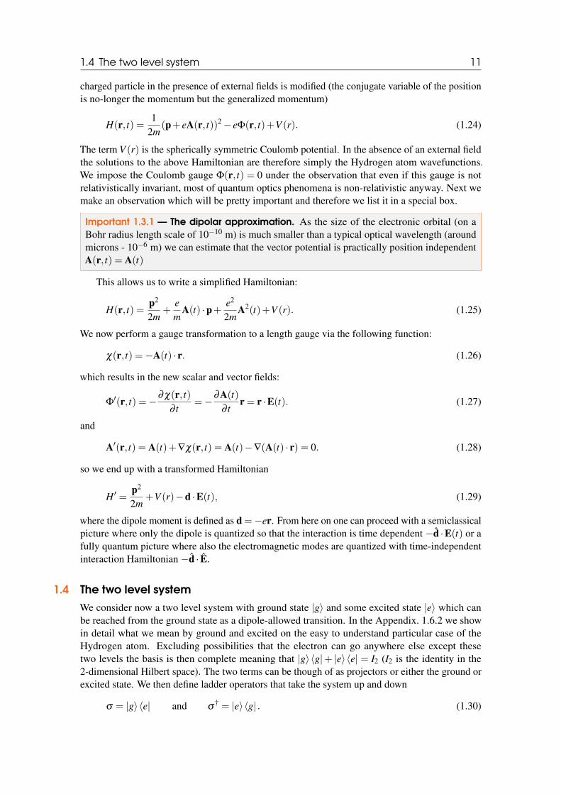
The term V (r) is the spherically symmetric Coulomb potential. In the absence of an external fieldthe solutions to the above Hamiltonian are therefore simply the Hydrogen atom wavefunctions.We impose the Coulomb gauge Φ(r, t) = 0 under the observation that even if this gauge is notrelativistically invariant, most of quantum optics phenomena is non-relativistic anyway. Next wemake an observation which will be pretty important and therefore we list it in a special box.

Important 1.3.1 — The dipolar approximation. As the size of the electronic orbital (on aBohr radius length scale of 10−10 m) is much smaller than a typical optical wavelength (aroundmicrons - 10−6 m) we can estimate that the vector potential is practically position independentA(r, t) = A(t)

This allows us to write a simplified Hamiltonian:

H(r, t) =p2

2m+

em

A(t) ·p+e2

2mA2(t)+V (r). (1.25)

We now perform a gauge transformation to a length gauge via the following function:

χ(r, t) =−A(t) · r. (1.26)

which results in the new scalar and vector fields:

Φ′(r, t) =−∂ χ(r, t)

∂ t=−∂A(t)

∂ tr = r ·E(t). (1.27)

and

A′(r, t) = A(t)+∇χ(r, t) = A(t)−∇(A(t) · r) = 0. (1.28)

so we end up with a transformed Hamiltonian

H ′ =p2

2m+V (r)−d ·E(t), (1.29)

where the dipole moment is defined as d =−er. From here on one can proceed with a semiclassicalpicture where only the dipole is quantized so that the interaction is time dependent −d ·E(t) or afully quantum picture where also the electromagnetic modes are quantized with time-independentinteraction Hamiltonian −d · E.

1.4 The two level systemWe consider now a two level system with ground state |g〉 and some excited state |e〉 which canbe reached from the ground state as a dipole-allowed transition. In the Appendix. 1.6.2 we showin detail what we mean by ground and excited on the easy to understand particular case of theHydrogen atom. Excluding possibilities that the electron can go anywhere else except thesetwo levels the basis is then complete meaning that |g〉〈g|+ |e〉〈e| = I2 (I2 is the identity in the2-dimensional Hilbert space). The two terms can be though of as projectors or either the ground orexcited state. We then define ladder operators that take the system up and down

σ = |g〉〈e| and σ† = |e〉〈g| . (1.30)


According to the Appendix. 1.6.2, the dipole moment operator does not have matrix elements on theindividual orbitals such that 〈g|d|g〉= 0 and 〈e|d|e〉= 0 We then can write the basis decompositionof the dipole moment operator as

d = |g〉dge 〈e|+ |e〉d∗ge 〈g| where dge = 〈g|d|e〉 . (1.31)

Finally we can now write the total Hamiltonian in terms of ladder operators as:

H = hωeσ†σ + hωg(1−σ

†σ)+

[σdeg ·E(t)+σ

†dge ·E(t)]

(1.32)

As we are free to substract a constant energy from the system, we will substract the term hωgI2and denote the energy diference ωe−ωg = ω0. Moreover, in some cases (see Appendix. 1.6.2) thetransition dipole moment element can be real: we will therefore, for simplicity, set deg = d∗eg = d.We can now write the final form of the free Hamiltonian plus the interaction with the field as

H = hω0σ†σ −d ·E(t)

[σ +σ

†] (1.33)

Next we will introduce another crucial approximation. To this end first we consider the case ofa classically driven TLS (as we mentioned before as a semiclassical picture). For an atom in theorigin a classical drive at frequency ω` is

E(t) = E` cos(ωLt)ε =E`

2(e−iω`t + eiω`t)ε. (1.34)

The semiclassical interaction then can be expressed as a sum of four terms:

Hint = h(d · ε)E`

2h

(σeiω`t +σ

†e−iω`t +σe−iω`t +σ†eiω`t

). (1.35)

First, we will denote the frequency (d · ε)E`/2h as the Rabi frequency. Most importantly, wewill perform a transformation into the Heisenberg picture (with the free Hamiltonian as shown inAppendix. 1.6.3):

HHPint = h

(d · ε)E`

2h

(σei(ω`−ω0)t +σ

†e−i(ω`−ω0)t +σe−i(ω`+ω0)t +σ†ei(ω`+ω0)t

). (1.36)

Notice that some terms are very quickly oscillating in time which means that their effectaverages to zero over any small interval much larger than 1/ω0. This allows us to make thefollowing statement:

Important 1.4.1 — Rotating wave approximation (RWA). One can neglect the quickly os-cillating terms in the dipole Hamiltonian and only keep terms showing detunings (frequencydifferences). The interaction Hamiltonian in the RWA then becomes

Hint = hΩ`

(σeiω`t +σ

†e−iω`t). where Ω` =

(d · ε)E`

2h. (1.37)

The same arguments apply to the fully quantum light-matter Hamiltonian. We can directlywrite it as

Hint = hω0σ†σ +∑

khωka†

kak +∑k

hgk

(akσ

† +σa†k

)(1.38)

where the coupling is

gk =

√hωk

2ε0Vd · εk

h=

Ekd · εk

h. (1.39)

1.5 Spontaneous and stimulated emission, stimulated absorption 13

Here the rotating wave approximation has a more direct interpretation. Terms like akσ† should beread as photon destroyed accompanied by an excitation of the TLS while its hermitian conjugateσa†

k shows the creation of a photon accompanying the de-excitation of the TLS. These are termsconserving energy. The terms which are equivalent with the counter-rotating terms discussed aboveare a†

kσ† with its hermitian conjugate. These terms are energy-non-conserving (creating photonswhile exciting the TLS).

1.5 Spontaneous and stimulated emission, stimulated absorptionLet us now analyze the fundamental processes through which a TLS inside the big quantizationbox can make transitions between the ground and excited states. First, let us assume an atom in theexcited state while the whole box is in the vacuum state except for a given specific mode which isalready occupied by a photon (with a given direction and polarization specified by a k0), i.e. westart with the state |e〉⊗ |0...1k0 ...0〉. The interaction Hamiltonian will then produce a sum of twostates

H |e〉⊗ |0...1k0 ...0〉= hgk0

√2 |e〉⊗ |0...2k0 ...0〉+ ∑

k 6=k0

hgk |e〉⊗ |0...1k0 ....1k..0〉 . (1.40)

The first one is a stimulated emission process where the first photon stimulates the emission of asecond photon in exactly the same direction and with the same polarization as the first one. Thesecond term is a spontaneous emission event where a photon is emitted in a random directionwith any polarization. which means that the atom gets de-excited while a photon is emitted into arandom direction with any polarization.Let us now start with an initially ground state TLS and a given specific one photon state, i.e. in thestate |g〉⊗ |0...1k0 ...0〉. The action of the Hamiltonian is then:

H |g〉⊗ |0...1k0 ...0〉= hgk0 |e〉⊗ |0...0...0〉 . (1.41)

The only possible process now is a stimulated absorption of the laser photon and subsequentexcitation of the atom.Notice that there are factors multiplying the transition probabilities for the stimulated processes, i.e.if we start with an arbitrary Fock state |0...nk0 ...0〉 the action of creation and annihilation operatorswill lead to an extra√nk0 or

√nk0 +1 factor. More generally, let us assume that the filled mode is

in a coherent state αk0 which will see that both the stimulated absorption and emission will havecollectively enhanced rates gk0αk0


1.6 Appendix1.6.1 Appendix A: The quantum harmonic oscillator

The one dimensional quantum harmonic oscillator is described by the following Hamiltonian

H =12

hω(P2 + Q2), (1.42)

where ω is the oscillation frequency while the two canonically conjugated operators fulfill thefollowing commutation relation [Q, P] = ih. For the electromagnetic field the dimensionless Q, Poperators have the meaning of quadratures associated with the electric and magnetic fields. Fora finite mass system, they are dimensionless position and momentum operators obtained via thefollowing transformations from the real momentum and position:

p = P√

mhω = pzpmP and x = Q

√h

mω= xzpmQ (1.43)

From here one can go further to define (non-hermitian) creation and annihilation operators:

a =1√2(Q+ iP) and a† =

1√2(Q− iP), (1.44)

where [a,a†] = 1 and the Hamiltonian becomes H = hω(a†a+ 12). Of course the inverse transfor-

mations are

Q =1√2(a+a†) and P =

i√2(a†−a) (1.45)

Number (Fock) basis. Displacement operator. Coherent states.The ground state is defined as the empty state |0〉 such that a |0〉 = 0. Fock (number states) arecreated by the continuous application of the creation operator onto the vacuum:

|n〉=√

1n!

a†n |0〉 , a |n〉=√

n |n−1〉 and a† |n〉=√

n+1 |n+1〉 . (1.46)

A special category of states, coherent states, are obtained by displacing the vacuum |α〉=Dα |0〉via the following operator

Dα = eαa†−α∗a = e−|α|2eαa†

e−α∗a. (1.47)

We have applied above the Baker-Hausdorff-Campbell formula

eA+B = eAeBe−[A,B]/2 when [A, [A,B]] = 0 and [B, [A,B]] = 0. (1.48)

One can then generally express the coherent state as a sum over the number states with Poissoniancoefficients

|α〉= e−|α|2

∞

∑n=0

αn√

n!|n〉. (1.49)

Notice a couple of useful properties such as

a|α〉= α|α〉, 〈α|a† = α∗〈α|, D†

αaDα = a+α, D†αa†Dα = a† +α

∗. (1.50)

Assuming that one wants to characterize the signal-to-noise ratio in a coherent state, the followingtwo expressions come in handy:

n = 〈α|a†a|α〉= |α|2 and ∆n =

√n2− n2 =

√n = |α|. (1.51)

For large amplitudes the average is much larger then the variance which means the signal-to-noiseratio n/∆n = 1/

√n = 1/|α| is extremely high. For quadratures notice that

Q =1√2(α +α

∗), Q =i√2(α∗−α), ∆Q = ∆P = 1/2. (1.52)

1.6 Appendix 15

Thermal statesA system in a pure state can be represented by a single ket and satisfies the Schrödinger equationih∂t |ψ〉 = H |ψ〉. One can as well rewrite the equation for the following quantity, the densityoperator or density matrix ρ = |ψ〉〈ψ| with the following von Neumann equation of motion:ih∂tρ = [H,ρ]. More generally however, the system is in a mixed state where the density matrix isexpressed as ρ = ∑ψ pψ |ψ〉〈ψ| which also satisfy the von-Neumann equation of motion.An example of a mixed state is the thermal state, where the density operator can be written as

ρth =e−H/kBT

Tr[e−H/kBT ]=

11− e−hω/kBT e−hωa†a/kBT . (1.53)

As a reminder, the trace is obtained by summing all the diagonal terms of the density matrix in theFock basis Tr[O] = ∑

∞n=0 〈n|O|n〉. Let’s compute the average occupancy in such a state (we will

make the notation β = hω/(kBT ):

n = Tr(ρtha†a) = (1− e−β )Tr[e−βa†aa†a] = (1− e−β )∞

∑n=0

ne−βn. (1.54)

We have used the property that the exponential of the Hamiltonian is diagonal in the number basis.In the above equation we can immediately see that the term (1− e−β )∑

∞n=0 ne−βn plays the role

of a probability distribution p(n). We will evaluate it after finding the expression for the average.Notice that the sum above is the derivative of the following sum.

∞

∑n=0

ne−βn =− ddβ

∞

∑n=0

e−βn =− ddβ

11− e−β

=e−β

(1− e−β )2 . (1.55)

This readily gives us the expected result of a Planck distribution average number and distribution

n =1

eβ −1=

1ehω/(kBT )−1

and pn =e−βn

1− e−β=

11− n

(n

1+ n

)n

(1.56)

We can also compute (exercise) the variance in a thermal state

[∆n]th =√

n+ n2. (1.57)

and remark that for large n this is at the level [∆n]th ' n which is much larger than the variance ofthe coherent state of [∆n]coh =

√n. Let us also remark h/kBT is around 10−11s at T = 1K, which

means that the exponent can very well be approximated (β 1→ eβ ' 1+β and the averagenumber is given by

n' hω

kBT. (1.58)

This is valid especially for small frequencies such as vibrations of membranes/mirrors, of ions in atrap, or acoustic phonons in a bulk solid. For high frequencies (optical frequencies of a mode in anoptical cavity, molecular vibrations etc) we have β 1 and the average occupancy is estimated by

n = e−hω/(kBT ). (1.59)

Notice that we can also re-express the density operator as

ρth =1

1+ n

∞

∑n=0

(n

1+ n

)n

|n〉〈n|. (1.60)


1.6.2 Appendix B: The hydrogen atom. Dipole allowed transitions.In general operator notations the problem of an electron (momentum and position operators p andr)orbiting around a (fixed - in a first, simplifying approximation) nucleus can be solved by solvingthe following Schrödinger equation

ih∂t |ψ〉= H |ψ〉 , with H =p2

2µ+V (r). (1.61)

Generally one separates time dependence from spatial dependence and then solves a time indepen-dent Schrödinger equation H |ψ〉= E |ψ〉 to get the solutions for the eigenvectors |nlm〉 indexed by(n, l,m). The indexes satisfy the following inequalities 1≤ n < ∞,0≤ `≤ n−1 and −`≤ m≤ `).

Denoting the eigenvalues of the Hamiltonian by Enlm the diagonal representation is Hamiltonianis then

H = ∑Enlm|nlm〉〈nlm|. (1.62)

The standard procedure is to turn the Schrödinger equation into a second order differential equation.This is done by writing it in the position representation where the position operator is replacedby the position parameter while the momentum is replaced by −ih∇. One then has to solve thefollowing differential equation:

ih∂

∂ tψ(r, t) =

[− h2

2µ∇

2 +V (r, t)]

ψ(r, t). (1.63)

Notice that the potential is assumed spherically symetric as is the case for the Coulomb interaction.Without further details we now state the well known results obtained for the Hydrogen atom(reducing the nucleus to a single proton). The eigenvalue and eigenvectors are

En =−

[µe4

32π2ε20 h2

]1n2 and ψnlml (r,θ ,φ) = 〈r|nlm〉= Rnl(r)Yl,m(θ ,φ). (1.64)

The energies only depend on the principal quantum number n (which will not be the case anylongerwhen one considers spin-orbit interactions, relativistic corrections etc). The radial part of thewavefunction for the Hydrogen atom (in reduced coordinate ρ = 2r/(na) is

Rnl(r) =−(

2na

)3 (n− l−1)!2n[(n+ l)!]3

ρlL2l+1

n+l (ρ)e−ρ/2. (1.65)

where the Bohr radius is a = 4πε0h2/(µe2) (µis the reduced mass roughly equal to the electronmass) and is around 0.529×10−10m.

The average orbital radius can be computed to give the result:

rnl = n2a0

[1+

12

(1− l(l +1)

n2

)](1.66)

An atom is normally found in the electronic ground state in the absence of light-induced excitations.For the Hydrogen atom the ground state is the 1s state. We will denote it by the ket |g〉. The statesclosest in energy are lying at energy differences close to h×1015 Hz. This means that for resonantexcitation we will need electromagnetic modes at optical frequencies around 1015 Hz. Now theatom is embedded in the vacuum which might be thermal. The vacuum is made by a collection of

1.6 Appendix 17

harmonic oscillators in thermal states and therefore with average occupancy n = e−hω/kBT . Let’sremember the constants h = 1.0545× 10−34m2kg/s and kB = 1.3806× 10−23m2kgs−2K−1. Wecan compute a useful quantity in kB/h = 1.309× 1011K−1s−1. Now we see that even at roomtemperature with T = 300K the value of n is pretty small as (1015Hz/(kBT/h) ' 10÷ 100. Inconclusion, thermal effects at such high frequencies do not play any role.Now we assume that we can somehow couple to state 2p in either of the degenerate sublevelsindexed by m =−1,0,1. Let’s select a single possible excited state and denote it by the ket |e〉. Wecan evaluate now the matrix elements of the dipole moment operator d =−er as follows

〈g|r|e〉=∫

dr∫

dr′〈g|r〉〈r|r|r〉〈r|e〉=∫

drψ∗g (r)rψe(r). (1.67)

Explicitly writing the integral in spherical coordinates for an unspecified m we get any of thesublevels of 2p∫ ∫ ∫

drdθdφ(r2 sinθ)

[2

1a3/2 e−r/2a 1√

4π

](xx+ yy+ zz)

[1

8√

31

a3/2

2r2a

e−r/2aY1,m(θ ,φ)

]=

(1.68)1√4π

14√

31a4

∫dr(r4)e−r/a

∫ ∫dθdφ(sinθ)(sinθ cosφ x+ sinθ sinφ y+ cosθ z)Y1,m(θ ,φ).

The m=0 case: For m = 0 the last integral over angles becomes√3

4π

∫ ∫dθdφ(sin2

θ cosφ x+ sin2θ sinφ y+ sinθ cosθ z)cosθ . (1.69)

We immediately see that the φ integration kills the contributions on x and y. The result is

2π

√3

4π

∫dθ sinθ cosθ

2z = 2π

√3

4π

23=

√4π

3. (1.70)

Putting it together

〈1s|r|2pz〉=1

12a4 .∫

dr(r4)e−r/az =1

12a4 .(24a5)z = 2az. (1.71)

The m= - 1 case: For m =−1 the last integral over angles becomes√3

8π

∫ ∫dθdφ(sin2

θ cosφ x+ sin2θ sinφ y+ sinθ cosθ z)sinθe−iφ . (1.72)

We immediately see that the φ integration kills the contribution on z. We then use∫

dφ cos2 φ =∫dφ sin2

φ = π and∫

dφ sinφ cosφ = 0. The integral above becomes\pi

π

√3

8π

[∫dθ sin3

θ(x− iy)]=

√3

4π

4π

3(x− iy) =

√4π

3(x− iy). (1.73)

n l m Orbital Rnl(ρ) Yl,m(θ ,φ)

1 0 0 1s 2 1a3/2 e−ρ/2 1√

4π

2 0 0 2s 12√

21

a3/2 (2−ρ)e−ρ/2 1√4π

1 -1 2p 18√

31

a3/2 ρe−ρ/2√

38π

sinθe−iφ

1 0 2p 18√

31

a3/2 ρe−ρ/2√

34π

cosθ

1 1 2p 18√

31

a3/2 ρe−ρ/2 −√

38π

sinθeiφ

Table 1.1: Energy levels and orbitals for the Hydrogen atom.


Putting it together

〈1s|r|2p−1〉= 2a(x− iy). (1.74)

The m= +1 case:For m = 1, similarly we get

〈1s|r|2p+1〉= 2a(x+ iy). (1.75)

1.6.3 Appendix C: Changing of picture (Interaction picture).Let us see how a change of picture is performed. Suppose we start with the Schrödinger equation:

ih∂t |ψ〉= H |ψ〉 , with H = hω0σ†σ + hΩ`

(σeiω`t +σ

†e−iω`t)

(1.76)

and aim at removing the time dependence in the driving part of the Hamiltonian. To this end wetransform into a different picture by a time dependent operator unitary U(t) such that |ψ〉IP =U(t) |ψ〉. Doing the proper transformations we end up with

ih∂t |ψ〉IP =[U(t)HU†(t)− ihU(t)∂tU†(t)

]|ψ〉IP . (1.77)

So we simply rewrote the Schrödinger equation in a different picture where the Hamiltonian isproperly modified as indicated above. Let us try our luck with the following choice for U(t) =e−iω`tσ†σ . The last term leads to a modification of the free Hamiltonian from hω0σ†σ to h(ω0−ω`)σ

†σ . The transformation of operators is a bit more complicated:

σIP =U(t)σU†(t) (1.78)

=

[1+−iω`t

1!σ

†σ +

(−iω`t)2

2!σ

†σ + ...

]σ

[1+

iω`t1!

σ†σ +

(iω`t)2

2!σ

†σ + ...

]=

(1.79)

= σ

[1+

iω`t1!

σ†σ +

(iω`t)2

2!σ

†σ + ...

]= σ

[1+

iω`t1!

+(iω`t)2

2!+ ...

]= σe−iω`t

(1.80)

We have used the properties σσ = 0 and σσ†σ =σ . Check them out! In the end, the transformationto the IP removes the fast time dependence in the driving Hamiltonian and one can write thefollowing Schrödinger equation: the Schrödinger equation for the transformed |ψ〉IP =U(t) |ψ〉(with U(t) = e−iH0t/h)

ih∂t |ψ〉IP = HIP |ψ〉IP with HIP = h(ω0−ω`)σ†σ + hΩ`

(σ +σ

†) (1.81)

2. The driven, decaying two level system

In the last chapter we discussed the quantization of light inside a box containing an infinite numberof modes (which we treated as plane waves) with wave vectors pointing in any direction. We thenadded a TLS and derived the light-matter interaction Hamiltonian. The dynamics of the system thenis unitary as excitations can flow from the field to the TLS and back. However, in reality we wouldlike to take the limit of an infinite box where a photon emitted by the TLS will practically neverreturn to it. To this end we perform an elimination of the box modes and derive the dynamics onlyin the 2-dimensional Hilbert space of the TLS. All other information about the electromagneticmodes is then uninteresting and the TLS dynamics becomes irreversible.

2.1 The quantum master equation for spontaneous emission

We start with an initial state density operator in the full Hilbert space of the TLS plus the infinitelymany electromagnetic modes. We assume that the initial state at some time t is separable and write

ρ(t) = ρA(t)⊗ρF(t). (2.1)

This could be the case for example by starting with the atom in state |e〉 and field in vacuum state atzero temperature such that ρF(t) = |0〉〈0| (the thermal bath case will be discussed later on). Also,the case where a coherent driving is present can be reduced to the vacuum case plus a classical termaccording to the Mollow transformation introduced in the previous chapter. More on this detail willbe presented later when we describe the Bloch equations.At some time t the total density operator fulfills the following equation of motion

dρ(t)dt

=− ih[H,ρ(t)]. (2.2)

where the Hamiltonian is the one derived in the previous chapter

H = hω0σ†σ +∑

khωka†

kak +∑k

hgk

(akσ

† +σa†k

), (2.3)

20 Chapter 2. The driven, decaying two level system

which one can break down into a sum of free evolution Hamiltonians HA and HF and the interactionpart. Remember the scaling of the coupling coefficients of each mode k with the two level systemincorporating the zero point electric field amplitude, the dipole transition element and the anglewith respect to the polarization of the respective electromagnetic mode:

gk =

√hωk

2ε0Vd · εk

h=

Ekd · εk

h. (2.4)

Let us now remove the free evolution part by moving into an interaction picture with a unitaryoperator U(t) = e−i(HA+HF )t/h (see Appendix 1.6.3) which transforms ρI =U†ρU and

HI = ∑k

hgk

[akσ

†ei(ω0−ωk)t +σa†ke−i(ω0−ωk)t

]= hF†(t)σ + hF(t)σ†. (2.5)

Notice that we have compactly written time dependent operators acting only on the photon statesand with the following properties

F(t) = ∑k

gkakei(ω0−ωk)t , F(t) |0〉= 0 and 〈0| F†(t) = 0. (2.6)

We can now write the von Neumann equation in the IP which looks exactly as before except thatthe Hamiltonian is the one above written in the IP. For simplicity of notation we will not write theindex I but still remember that until the end of the derivation we stay in the IP. Let us then proceedby formally integrating the equation of motion for the density operator in a small interval ∆t (wewill clarify towards the end of the derivation how small the interval actually is - compared to othertimescales involved in the problem):

dρ(t)dt

=− ih[HI(t),ρ(t)] → ρ(t +∆t) = ρ(t)− i

h

∫ t+∆t

tdt1[HI(t1),ρ(t1)], (2.7)

For any moment in time such that t < t1 < t + ∆t we can again write the formal solution asρ(t1) = ρ(t)−

∫ t1t dt2[HI(t2),ρ(t2)] and plug it back in the above expression to get

ρ(t +∆t) = ρ(t)− ih

∫ t+∆t

tdt1[HI(t1),ρ(t)]−

1h2

∫ t+∆t

tdt1∫ t1

tt2[HI(t1), [HI(t2),ρ(t2)].

(2.8)

This is still exact. We can now continue dividing the interval even further in the following orderedsequence t < ...t3 < t2 < t1 < t +∆t and obtain more and more terms in the expansion above.However, assuming that the field-TLS couplings are small compared to the energies of the TLS orthe field modes, a truncation at the second order level suffices as a perturbative approach. This isequivalent to replacing ρ(t2) with ρ(t) in the above formula and obtain the following equation

ρ(t +∆t) = ρ(t)− ih

∫ t+∆t

tdt1

ih[HI(t1),ρ(t)]−

1h2

∫ t+∆t

tdt1∫ t1

tdt2[HI(t1), [HI(t2),ρ(t)].

(2.9)

Since we are only interested in the state of the TLS and not of the bath we would like to re-writethe above equation into an effective equation for ρA = TrF [ρ]. This means we will have to performtraces like TrF [HI(t1),ρA(t)⊗ρF(t)] and TrF [HI(t1), [HI(t2),ρA(t)⊗ρF(t)].

First order tracesRemember that ρF(t) = |0〉〈0| which means that in the following trace TrF [HI(t1),ρA(t)⊗ρF(t)]only the vacuum state survives. This is easily seen by explicitly writing the trace: TrF [HI(t1),ρA(t)⊗ρF(t)] = ∑n 〈n| [HI(t1),ρA(t)⊗ρF(t)] |n〉. Using 〈n|0〉= δn,0 we end up with

TrF [HI(t1),ρA(t)⊗ρF(t)] = 〈0|HI(t1)|0〉ρA(t)−ρA(t)〈0|HI(t1)|0〉= 0. (2.10)

2.1 The quantum master equation for spontaneous emission 21

Second order tracesLet’s explicitly separate the second order terms coming from the double commutator [HI(t1), [HI(t2),ρ(t)]into 4 distinct parts:

T1 = TrF [HI(t1)HI(t2)ρA(t)⊗ρF(t)] , (2.11)

T2 =−TrF [HI(t1)ρA(t)⊗ρF(t)HI(t2)] , (2.12)

T3 =−TrF [HI(t2)ρA(t)⊗ρF(t)HI(t1)] , (2.13)

T4 = TrF [ρA(t)⊗ρF(t)HI(t2)HI(t1)] . (2.14)

Before evaluating the terms above we can observe a few simplifying rules. With the resultsF(t) |0〉 = 0 and 〈0|F†(t) = 0 it means that we can reduce some terms like HIρF = hσF† andρFHI = hσF . Moreover the field operators do not act on ρA so we can commute them. Let’s thenwork out the first term T1 according to these rules

T1 = h2TrF [(F†(t1)σ +F(t1)σ†)

σF†(t2)ρA(t)⊗ρF(t)] (2.15)

= h2σ

†σρATrF

[F(t1)F†(t2)ρF(t)

]. (2.16)

Similarly we can find:

T2 =−h2σρAσ

†TrF [F(t1)F†(t2)ρF(t)], (2.17a)

T3 =−h2σρAσ

†TrF [F(t2)F†(t1)ρF(t)], (2.17b)

T4 = h2ρAσ

†σTrF [F(t2)F†(t1)ρF(t)]. (2.17c)

We see that in the end we are left with the task of evaluating bath correlations at different times andthen integrate over them. For example, the term coming from T1 will be

B =∫ t+∆t

tdt1∫ t1

tdt2TrF [F(t1)F†(t2)ρF(t)]. (2.18)

Also notice that inversing the time ordering has the effect of a complex conjugate: TrF [F(t2)F†(t1)ρF(t)]=TrF [F(t1)F†(t2)ρF(t)]∗. Adding everything up we can find a compact expression connecting thereduced density operator at two different times:

ρA(t +∆t)−ρA(t) = (B+B∗)σρA(t)σ†−σ†σρA(t)B−ρA(t)σ†

σB∗. (2.19)

A closer inspection of the terms inside the B coefficient show that they are not too hard to evaluateand understand. Writing in detail

TrF[F(t1)F†(t2)ρF(t)

]= 〈0|∑

k∑k′

gkg∗k′aka†k′e

i(ω0−ωk)t1e−i(ω0−ω ′k)t2 |0〉 (2.20)

= ∑k|gk|2ei(ω0−ωk)(t1−t2). (2.21)

We have used the fact that aka†k′ |0〉= δkk′ |0〉 to reduce to a single sum. Putting it all together we

again see that the task is to evaluate the following quantity

B = ∑k|gk|2

∫ t+∆t

tdt1∫ t1

tdt2ei(ω0−ωk)(t1−t2). (2.22)

This we can do in two steps: first summing over all k-vectors and polarizations and then performingthe time integral.


Summing over k-vectors and polarizationsTo evaluate the sum we will write it as an integral. The general rule for turning a sum into anintegral is

∑k|gk|2...= ∑

λ

∫dk|gk|2D(k)..., (2.23)

where D(k) is a function also called density of states, which should verify that we count everythingcorrectly. It is obvious that for the sum to integral transformation to be valid it should satisfy thefollowing condition within a given volume in k-space

∑k

1 = ∑λ

∫dkD(k), (2.24)

Let us notice that as we quantized the field in a box of dimensions L×L×L the allowed k-vectorcomponents on a given axis are separated by 2π/L. Therefore we will only find one k-vector with agiven polarization within a volume (2π/L)(2π/L)(2π/L)×8∗π3/V . Writing the above conditionthen results in 2 = D(k)8∗π3/V which readily gives

D(k) =V

4π3 . (2.25)

The term stemming from the coupling is expressed as

|gk|2 =ωk

2hε0V(d · εk)

2. (2.26)

For any given direction defined the unit vector k, the three unit vectors ε(1)k , ε

(2)k and k are orthonor-

mal and thus constitute a basis. Therefore we can write d = (d · ε(1)k )ε

(1)k +(d · ε(2)

k )ε(2)k +(d · k)k

and consequently the amplitude squared |d|2 = (d · ε(1)k )2+(d · ε(2)

k )2+(d · k)2. We can then express

∑λ

|gk|2 =ωk

2hε0V

[|d|2− (d · k)2] . (2.27)

Assuming the d points out in the z direction, we effectively have |d|2− (d · k)2 = |d|2(1− cos2 θ).Now we can write the integral

∑λ

∫dk|gk|2D(k)...=

V4π3

∫ 2π

0dφ

∫π

0dθ sinθ(1− cos2

θ)∫

∞

0dkk2 ωk|d|2

2hε0V... (2.28)

=|d|2

8π3hε0

∫ 2π

0dφ

∫π

0dθ sinθ(1− cos2

θ)∫

∞

0dkk2

ωk..., (2.29)

and already perform the angle integral∫ 2π

0 dφ∫

π

0 dθ sinθ(1− cos2 θ) = 2π(4/3) = 8π/3 leadingto

∑λ

∫dk|gk|2D(k)...=

|d|2

8π3hε0

8π

3

∫dkk2

ωk...=|d|2

3π2c3hε0

∫dωkω

3k .... (2.30)

Performing the time integralWe finally get to the time dependant part as we can state

B =|d|2

3π2c3hε0

∞∫0

dωk

t+∆t∫t

dt1

t1∫t

t2e−i(ωk−ω0)(t1−t2)ω3k . (2.31)

2.1 The quantum master equation for spontaneous emission 23

Let us rewrite it for clarity with the transformation ωk−ω0 = x (and noticing that as ω0 is a veryhigh frequency we can extend the integration over to −∞)

B =|d|2

3π2c3hε0

∞∫−∞

dx∆t∫

0

dt1e−ixt1

t1∫0

t2eixt2(x+ω0)3 =

|d|2

3π2c3hε0I (∆t), (2.32)

We also removed the lower bound t to zero as the initial time is irrelevant in the integral. Noticethat the exponential oscillates and averages the polynomial to zero unless x is around the origin.proceed with the first integral, where caution has to be taken as a singularity appears at x = 0. Wewill deal with this by the following trick:

t1∫0

t2eixt2(x+ω0)3 = lim

ε→0

∫ t1

0t2eixt2−εt2(x+ω0)

3 = limε→0

(x+ω0)3

ix− ε

(eixt1−εt1−1

)= (2.33)

Plugging it back into the integral

I (∆t) =∞∫−∞

dx∆t∫

0

dt1 limε→0

(x+ω0)3

ix− ε

(e−εt1− e−ixt1

). (2.34)

If ∆t is very large (can be taken to infinity), the last contribution is averaged to zero (the one frome−ixt1). The first contribution can be rewritten:

limε→0

−(ix+ ε)(x+ω0)3

x2 + ε2 = limε→0

−(ix+ ε)(x+ω0)3

x2 + ε2 = (2.35)

=−limε→0

ε

x2 + ε2 (x+ω0)3− ilim

ε→0

xx2 + ε2 (x+ω0)

3. (2.36)

The limits make sense as distributions. The real part becomes a delta function

limε→0

ε

x2 + ε2 = πδ (x), (2.37)

while the imaginary part becomes the principal value distribution

limε→∞

xx2 + ε2 = P(

1x

), (2.38)

defined (in the sense of a distribution thus acting on test functions) as∫∞

−∞

dxP(1x

)f(x) = limε→0

[∫ −ε

−∞

dx+∫

∞

ε

dx]f (x)

x. (2.39)

The principal part (as one can for example check numerically for safety) makes very little contribu-tion. Keeping the delta function only one obtains:

I (∆t) = πω30 ∆t. (2.40)

Finally we can put everything together and find that the coefficient B in the density operatorevolution is proportional to the small time increment

B =

[|d|2ω3

03πc3hε0

]∆t. (2.41)


Final resultFinally, as the terms in the right side of the master equation are real and proportional to ∆t, wecan write we can express the master equation as ρA(t +∆t)−ρA(t) = ∂tρA(t)∆t. Moreover, wewill now transform back from the interaction picture and write a very simple form for the masterequation (written below in the Schrödinger picture)

Important 2.1.1 — The master equation for spontaneous emission.

ddt

ρA =− ih[HA,ρA]+ γ

2σρAσ

†−ρAσ†σ −σ

†σρA

. (2.42)

A few words on this. Without the box, the atom simply evolves in a coherent, deterministic waygoverned by the free Hamiltonian HA. The interaction with the box brings along an infinity of termsdescribing the coupling of the TLS with any of the electromagnetic modes supported by the box.The trace over the bath modes leads to an irreversible dynamics contained in the super-operatorLinbdlad term that describes the non-trivial action of the collapse operator σ at rate γ on thedensity operator. The action is non-trivial as it cannot be represented as a matrix multiplication. Insimplified notation we can also write

ddt

ρA =− ih[HA,ρA]+ γD [σ ,ρA] with D [σ ,ρA] = 2σρAσ

†−

ρA,σ†σ+. (2.43)

where the brackets indexed by a plus sign show the anticommutator.The quantity in the brackets is the spontaneous emission rate of a two-level system into theelectromagnetic vacuum modes:

γ =|d|2ω3

03πc3hε0

. (2.44)

Let’s check out the value of the decay rate for the Hydrogen 1s to 2p transition. The constants are:h = 1.055× 10−34m2s−1kg, c = 3× 108m/s, ε0 = 8.85× 10−12A2s4kg−1m−3. The 1s energy is−13.6eV while the 2p energy is roughly −13.6/4 eV. We can equate hω0 = 3/4×13.6×1.602×10−19J to obtain ω0 = 1.139×1015 Hz. Remembering from the first lecture that for the z-polarizedtransition, the dipole matrix element is 2a0e where the Bohr radius is a0 = 0.53×10−10 m, we cancompute γ = 1.79×106 Hz, so on the order of MHz.

Master equation in a thermal bathThe calculation performed on an initial vacuum state of the bath can be easily extended to athermally occupied bath at temperature T and with an average photon number occupancy n(ω0).For such a bath we can write the initial density operator

ρF(t) =e−HF/(kBT )

TrF [e−HF/(kBT )]= ∏

k

e−nkhωk/(kBT )

1− e−hωk/(kBT )|nk〉〈nk|. (2.45)

Without going into the details of the derivation notice that the only step where a difference occursis the calculation of the correlations of the bath. These correlations will give rise to a modifiedemission rate and an extra term showing the possibility that the bath can induce absorption. In shortone obtains:

ddt

ρA =− ih[HA,ρA]+ γ (n(ω0)+1)D [σ ,ρA]+ γ n(ω0)D [σ†,ρA]. (2.46)

The Linblad term with collapse operator σ contains the expected spontaneous emission term towhich a thermally activated stimulated emission is added. The second Linblad term has a collapse

2.2 Bloch equations (in the Schrödinger picture) 25

operator σ† showing inverse decay from the ground to the excited state, i.e. stimulated absorptionfrom the thermal bath. As we mentioned before, typically we will deal with optical transitionwhere even at room temperature n(ω0) 1 such that we will not make too much use of the aboveexpression.

Alternative derivation of the decay rateOne can use a variety of methods to derive the spontaneous emission rate. For example, sometextbook are using the so-called Wigner-Weisskopf derivation. We can sketch another simpleintuitive derivation by making use of the Fermi’s golden rule for the computation of the transitionprobability between states |e,0〉 and |g,1k〉 for any possible direction and polarization of the emittedphoton. We use

we→g =2π

h2 ∑k|〈e,0|Hint |g,1k〉|2δ (ωk−ω0) = (2.47)

= 2π ∑k

∑k′

∑k′〈e,0|Hint |g,1k〉〈g,1k|Hint |e,0〉δ (ωk−ω0) =

= 2π ∑k〈e,0|gk′ak′σ

†|g,1k〉〈g,1k|gk′′a†k′′σ |e,0〉δ (ωk−ω0) =

= 2π ∑k|gk|2δ (ωk−ω0) =

2π|d|2

3π2c3hε0

∫dωkω

3k δ (ωk−ω0) =

=2|d|2ω3

03πc3hε0

= γ.

Notice that the rate obtained at which the system emits spontaneously is exactly twice the rate wecomputed before via the master equation derivation.

2.2 Bloch equations (in the Schrödinger picture)

We now know how the effect of the interaction with the vacuum on a TLS can be mathematicallydescribed. The resulting dynamics in the reduced Hilbert space of dimension 2 is irreversible andcharacterized by the action of a super-operator onto the density operator. Let us now add a coherentdrive and check out the resulting driven-dissipative dynamics. This can be done as described in thefirst chapter by assuming one of the field modes to be in a coherent state characterized by a givendirection k0 including a given polarization εk0 . After performing the Mollow transformation oneends up with the effect of the drive as a semiclassical Hamiltonian (H`) added to the free evolutionHamiltonian (H0):

H = hω0σ†σ + hΩ

(σeiω`t +σ

†e−iω`t). (2.48)

The Rabi frequency depends on the amplitude of the coherent states as well as on the transitiondipole moment and its overlap with the light mode polarization vector:

Ω =1hEk0αk0d · εk0 (2.49)

We now can follow the evolution of the system in the Schrödinger picture by solving the completeequation of motion for the density operator (we drop in the following the A subscript but rememberwe are always working in the 2-dimensional Hilbert space of the TLS):

ddt

ρ =− ih[H,ρ]+ γ

2σρσ

†−ρσ†σ −σ

†σρ. (2.50)


Derivation starting from the density operatorNotice that in the Hilbert space spanned by the two basis states |g〉 and |e〉 the density operator hasfour matrix elements. The elements are computed the usual way as sandwiches between bras andket, for example: ρeg = 〈e|ρ |g〉. Let us as an example compute the evolution of ρeg. To this endwe sandwich the master equation above between 〈e| and |g〉:

ddt

ρeg =−ih〈e| [H,ρ] |g〉+ γ

2〈e|σρσ

† |g〉−〈e|ρσ†σ |g〉−〈e|σ†

σρ |g〉. (2.51)

We now remember the action of operators on the ladder operators on states σ |e〉= |g〉, σ |g〉= 0,σ† |e〉= 0, σ† |g〉= |e〉 and so on. Let’s break the terms down in 3 parts. Free evolution gives

− ih〈e| [H0,ρ] |g〉=−iω0 〈e|

(σ

†σρ−ρσ

†σ)|g〉=−iω0ρeg. (2.52)

The drive terms leads to the following contribution:

− ih〈e| [H`,ρ] |g〉=−iΩ〈e|(σeiω`t +σ

†e−iω`t)ρ−ρ(σeiω`t +σ†e−iω`t) |g〉 (2.53)

=−iΩ〈g|e−iω`tρ |g〉+ iΩ〈e|e−iω`tρ |e〉= iΩ(ρee−ρgg)e−iω`t

Finally, the spontaneous emission gives rise to

γ

2〈e|σρσ† |g〉−〈e|ρσ

†σ |g〉−〈e|σ†

σρ |g〉=−γρeg. (2.54)

Putting it all together we obtain an equation of motion for the ’coherence’ ρeg showing free evolutionat frequency ω0, driving with strength Ω and frequency ω` and decay at amplitude decay rate γ

ddt

ρeg =−γρeg− iω0ρeg + iΩ(ρee−ρgg)e−iω`t . (2.55)

Notice that the drive depends on the population difference between excited state ρee and groundstate ρgg. One can continue in deriving the equations for the other elements. Notice that sincethe trace of the density operator is conserved then ρee +ρgg = 1. This basically means that thepopulation can only be in one of the two states of the system. Also notice that ρge = ρ∗eg. In effectwe only have to compute the excited state population evolution equation which we list below:

ddt

ρee =−2γρee + iΩ(ρegeiω`t −ρgee−iω`t). (2.56)

Derivation on the level of the density matrixA more direct way to obtain all the equations is to make use of the matrix representation of thedensity operator, i.e. the density matrix formalism. We start by representing the states as vectorsand properly writing the density operator as a matrix in this basis:

|g〉 →[

01

]|e〉 →

[10

]and ρ =

[ρee ρeg

ρge ρg

]. (2.57)

It is the straightforward to write the ladder operators as well as the projectors into the excited andground state as matrices as well:

σ =

[0 01 0

]σ

† =

[0 10 0

]σ

†σ =

[1 00 0

]σσ

† =

[0 00 1

], (2.58)

2.3 Bloch equations (in the Heisenberg picture) 27

and check that they perform the required tasks by multiplying them with the state vectors. The freeand driving Hamiltonians are then written as

H0 =

[hω0 0

0 0

], H` =

[0 hΩe−iω`t

hΩeiω`t 0

], (2.59)

from which one can derive the Hamiltonian part of the master equation from matrix multiplications.

− ih[H,ρ] =

[iΩ(ρegeiω`t −ρgee−iω`t) −iω0ρeg + iΩe−iω`t(ρee−ρgg))

−iω0ρge−+iΩeiω`t(ρee−ρgg)) −iΩ(ρegeiω`t −ρgee−iω`t)

](2.60)

Notice that the Lindblad part gives rise to the following matrix on the rhs of the master equation:

γD [σ ,ρ] =

[−2γρee −γρeg

−γρge 2γρee

](2.61)

Important 2.2.1 — Bloch equations. Putting it all together we get a set of equations describingthe free evolution, effect of driving and spontaneous emission of a single TLS:

∂tρee =−2γρee + iΩ(t)(ρegeiω`t −ρgee−iω`t), (2.62a)

∂tρeg =−γρeg− iω0ρeg + iΩ(t)(ρee−ρgg)e−iω`t . (2.62b)

Remember that the other two matrix elements are derived from ρee +ρgg = 1 and ρge = ρ∗eg.

We can easily remove the time dependence by moving into a rotating frame, procedure which isequivalent of saying that we write equations only for the slowly varying envelopes ρeg = ρege−iω`t .Notice that ∂tρeg = ∂t ρege−iω`t− iω`ρeg. We end up with rewriting equations of motion in a rotatingframe and with defined detuning: ∆ = ω0−ω`. I’ll drop the tilde since it takes forever to type it inlatex :)

∂tρee =−2γρee + iΩ(t) [ρeg−ρge] , (2.63a)

∂tρeg =−γρeg− i∆ρeg + iΩ(t)(ρgg−ρee) . (2.63b)

2.3 Bloch equations (in the Heisenberg picture)An equivalent procedure is to solve not for the density operator time evolution but instead to deriveequations of motion for single or more operator averages. For example let us compute the evolutionfor 〈σ〉(t) = Tr[σρ(t)]. We notice that ∂t 〈σ〉(t) = ∂tTr[σ(t)ρ(0)] = ∂tTr[σρ(t)] = Tr[σ∂tρ(t)]which means we can now use the master equation to write

∂t 〈σ(t)〉= Tr[

σ(− ih[H,ρ]+ γ

2σρAσ

†−ρσ†σ −σ

†σρ)

](2.64)

=−iω0 〈σ(t)〉− γ 〈σ(t)〉+ iΩe−iω`t 〈σ†σ −σσ

†〉 .

As one can observe that 〈σ〉(t) = Tr[|g〉〈e|ρ(t)] = 〈e|ρ(t) |g〉 = ρeg(t) the equation above is nosurprise.

2.4 Time dynamics of the driven-dissipative TLSWe will now analyze the time dynamics imposed by the above equations under different conditions.We will mainly distinguish between resonant versus off-resonant driving, coherent versus incoherentevolution, transient versus steady state dynamics and linear versus non-linear regimes.


0 2 4 6 80.0

0.2

0.4

0.6

0.8

1.0

time

pex

c

0 2 4 6 80.0

0.2

0.4

0.6

0.8

1.0

time

pex

c

0 5 10 15 20 25 300.0

0.2

0.4

0.6

0.8

1.0

time

pex

c

0 1 2 3 40.0

0.2

0.4

0.6

0.8

1.0

time

pex

c

0 1 2 3 40.0

0.2

0.4

0.6

0.8

1.0

time

pex

c

0.0 0.5 1.0 1.5 2.00.0

0.2

0.4

0.6

0.8

1.0

Rabi - frequency

pex

c

Figure 2.1: Response of a TLS under driving and decay.

Rabi oscillationsWe now focus on the purely coherent dynamics of a drive system (no dissipation included). Westart with the equations of motion after the removal of the fast optical oscillations such that

∂tρee = iΩ(t) [ρeg−ρge] , (2.65a)

∂tρeg =−i∆ρeg + iΩ(t)(ρgg−ρee) , (2.65b)

∂tρge = i∆ρge− iΩ(t)(ρgg−ρee) . (2.65c)

We can simplify things a bit by the following notations: X = ρeg + ρge, Y = i(ρeg− ρge) andZ = ρee−ρgg. In terms of these three (real) values one can write

∂tZ = 2Ω(t)Y, (2.66a)

∂tX =−∆Y (2.66b)

∂tY = ∆X +Ω(t)Z. (2.66c)

ddt

ρge =−γ

2ρge + i∆ρge− iΩ(t)(ρgg−ρee) , (2.67)

allows us to derive the real and imaginary parts evolving as

ddt(ρge +ρeg) =−

γ

2(ρge +ρeg)+ i∆(ρge−ρeg) (2.68)

ddt(ρge−ρeg) =−

γ

2(ρge−ρeg)+ i∆(ρge +ρeg)−2iΩ(t)(1−2ρee) . (2.69)

For a simple solution we now focus on resonance where only two equations are consequentlycoupled.

ddt

ρee =−γρee− iΩ(t) [ρge−ρeg] , (2.70)

2.4 Time dynamics of the driven-dissipative TLS 29

ddt(ρge−ρeg) =−

γ

2(ρge−ρeg)−2iΩ(t)(1−2ρee) . (2.71)

In vector form one can write:

ddt

[ρee

ρge−ρeg

]=

[−γ −iΩ(t)

4iΩ(t) −γ/2

][ρee

ρge−ρeg

]+

[0

−2iΩρee

]. (2.72)

The solutions from above are pretty complicated. The physics is pretty straighfoward though.We will first set γ to zero, set the Rabi driving time independent and check the existense of Rabioscillations and their period. Consider again:

ddt(ρgg−ρee) = 2iΩ [ρge−ρeg] , (2.73)

ddt(ρge−ρeg) =−2iΩ(ρgg−ρee) . (2.74)

Taking the double derivative of the first expression we get

d2

dt2 (ρgg−ρee) = 2iΩ [−2iΩ(ρgg−ρee)] , (2.75)

which turns into a driven harmonic oscillator problem:

d2

dt2 (ρgg−ρee)+4Ω2(ρgg−ρee) = 0, (2.76)

with solutions (ρgg−ρee)(t) = Acos2Ωt +Bsin2Ωt. Let’s consider an initial ground state atomsuch that (ρgg−ρee)(0) =−1. Also the coherences are vanishing at zero time meaning that the Bterm is zero. The following evolution will be

(ρgg−ρee)(t) =−cos2Ωt. (2.77)

A so-called pi pulsecan be achieved when 2Ωt = π such that (ρgg−ρee)(t = π/(2Ω) =−1) andthe population has been completely transferred in the excited state. For 2Ωt = π/2 a pi/2 pulse isrealized where t (ρgg−ρee)(t = π/(4Ω) = 0) but the coherence between the levels is maximal.

π and π/2 pulsesRate equations and steady state solutionsWe now include spontaneous emission and look at the dynamics on a timescale larger than γ−1

where we can in a first step we can eliminate the dynamics of the coherence ρeg by setting itsderivative to zero. We then obtain(for simplicity we assume constant driving)

∂tρee =−2γρee− iΩ [ρge−ρeg] , (2.78a)

ρeg =iΩ

γ + i∆(ρgg−ρee) (2.78b)

After a few steps one can check that the population equation becomes

ddt

ρee =−γ

[1+

2Ω2

γ2 +∆2

]ρee +

γΩ2

γ2 +∆2 , (2.79)


-10 -5 0 5 100.0

0.2

0.4

0.6

0.8

1.0

detuningp

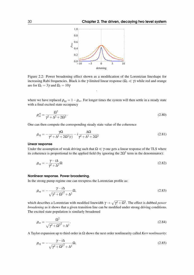
exc

Figure 2.2: Power broadening effect shown as a modification of the Lorentzian lineshape forincreasing Rabi frequencies. Black is the γ-limited linear response (Ω` γ) while red and orangeare for Ω` = 3γ and Ω` = 10γ

.

where we have replaced ρgg = 1−ρee. For longer times the system will then settle in a steady statewith a final excited state occupancy

ρssee =

Ω2

γ2 +∆2 +2Ω2 . (2.80)

One can then compute the corresponding steady state value of the coherence

ρeg =−γΩ

γ2 +∆2 +2Ω2(t)− i

∆Ω

γ2 +∆2 +2Ω2 (2.81)

Linear responseUnder the assumption of weak driving such that Ω γ one gets a linear response of the TLS whereits coherence is proportional to the applied field (by ignoring the 2Ω2 term in the denominator):

ρeg =−γ− i∆

γ2 +∆2 Ω (2.82)

Nonlinear response. Power broadening.In the strong pump regime one can reexpress the Lorentzian profile as:

ρeg =−γ− i∆√

γ2 +Ω22+∆2

Ω, (2.83)

which describes a Lorentzian with modified linewidth γ →√

γ2 +Ω2. The effect is dubbed powerbroadening as it shows that a given transition line can be modified under strong driving conditions.The excited state population is similarly broadened

ρee =Ω2√

γ2 +Ω22+∆2

. (2.84)

A Taylor expansion up to third order in Ω shows the next order nonlinearity called Kerr nonlinearity:

ρeg =−γ− i∆√

γ2 +Ω22+∆2

Ω, (2.85)

2.5 Application: population inversion in three level systems 31

2.5 Application: population inversion in three level systemsThe previous section has already shown that a population inversion cannot be established in a twolevel system under steady state conditions. However we can consider a more complicated situationwhere driving is performed indirectly via an intermediate level |i〉 aimed to provide inversionbetween the main |g〉 and |e〉 states (see Fig). We now make use of the formalism developed forTLS to apply it for each pair of levels. The Hamiltonian of the system is:

H = hω0 |e〉〈e|+ h(ω0 +ν) |i〉〈i|+ hΩ[|g〉〈i|eiω`t + |i〉〈g|e−iω`t

]. (2.86)

To this we add all the damping processes as usual Lindblad terms with the proper rate and collapseoperator specifications

∂tρ =− ih[H,ρ]+ γiD [|g〉〈i| ,ρ]+ γD [|g〉〈e| ,ρ]+ΓD [|e〉〈i| ,ρ] (2.87)

One can proceed with deriving the following set of Bloch equations by using the rules we havederived for the closed two level system case:

∂tρee =−2γρee +Γρii, (2.88)

∂tρeg = iδρeg−γe

2ρeg + iΩρe1, (2.89)

∂tρgg = γeρee + γ1ρ11 + iΩ [ρg1−ρ1g] , (2.90)

∂tρ11 =−γ1ρ11− γnrρ11− iΩ [ρg1−ρ1g] , (2.91)

∂tρ1g =−γnr + γ1

2ρ1g− iΩ(ρgg−ρ11) , (2.92)

∂tρe1 = iδρe1−γ1 + γe + γnr

2ρe1 + iΩρeg. (2.93)

We want to close the equations for the e-g system under the condition that γnrΩ,γ1g,γeg. Noticethat we can transform both ρeg and ρe1 with δand eliminate

ρe1 =2iΩ

γ1 + γe + γnrρeg. (2.94)

In a rotating frame we get

ddt

ρeg = iδρeg−γe

2ρeg−

2Ω2

γ1 + γe + γnrρeg. (2.95)

Now we eliminate

ρ1g =2iΩ

γnr + γ1(ρgg−ρ11) , (2.96)

leading to

iΩ [ρg1−ρ1g] =4Ω2

γnr + γ1(ρgg−ρ11) , (2.97)

and subsequently

ρ11 =4Ω2

(γnr + γ1)2 (ρgg−ρ11) , (2.98)

which results in

ρ11 =4Ω2

4Ω2 +(γnr + γ1)2 ρgg. (2.99)


The effective two-level modelPlugging all this back into the equations we get:

ddt

ρee =−γegρee +4Ω2γnr

4Ω2 +(γnr + γ1g)2 ρgg, (2.100)

ddt

ρeg =−(

γe

2+

2Ω2

γ1 + γe + γnr

)ρeg, (2.101)

ddt

ρgg = γegρee−4Ω2γnr

4Ω2 +(γnr + γ1g)2 ρgg. (2.102)

Under typical conditions, γnr γe,γ1 and Ω γnr , we can simplify to a common pump rate

Γ≈ 4Ω2

γnr, (2.103)

and write the following equations: Plugging all this back into the equations we get:

ddt

ρee =−2γegρee +2Γρgg, (2.104)

ddt

ρeg =−(γe +Γ)ρeg. (2.105)

ddt

ρgg = γegρee−Γρgg. (2.106)

This is exactly a model for incoherent pumping (or inverse decay). We can rewrite it as:

ρ =− ih[H0,ρ]+ γeD[|g〉〈e|,ρ]+ΓD[|e〉〈g|,ρ]. (2.107)

Let’s check out if this is true:

ρeg = 〈e|Γ [|2e〉〈g|ρ|g〉〈e|− |g〉〈g|ρ−ρ|g〉〈g|] |g〉=−Γρeg. (2.108)

2.6 Appendix: The Bloch sphere 33

2.6 Appendix: The Bloch sphereAnticipating the discussion in Chapter 7 on qubit operations in ion traps let us encode the 0 and 1qubits in the internal levels |0〉 ≡ |g〉 and |1〉 ≡ |e〉 of a two level system. We will in the followingfollow a matrix approach where we denote:

|0〉 ≡[

01

]and |1〉 ≡

[10

](2.109)

For any pure state we can form the most general superposition as:

|ψ〉= cosθ

2|1〉+ eiφ sin

θ

2|0〉. (2.110)

This can be vizualized on a unit sphere surface as a point described by a Bloch vector:

a = (sinθ cosφ ,sinθ sinφ ,cosθ) = (X ,Y,Z). (2.111)

More generally, states can be mixed and then they are described by density operators. A densityoperator in a 2×2 space can be written uniquely as a combination of the identity matrix and threeindependent Pauli matrices (as they form a complete basis in this Hilbert space)

ρ =12(I2 +a ·σ) =

12

[1+Z X− iY

X + iY 1−Z

]=

[ρ11 ρ10ρ01 ρ00

], (2.112)

where by definition

σx =

[0 11 0

]= σ +σ

†, (2.113a)

σy =

[0 −ii 0

]= i(σ −σ

†), (2.113b)

σz =

[1 00 −1

]= σ

†σ −σσ

†. (2.113c)

Now we have 3 independent parameters translatable to two angles and a radius: the correspondingBloch vector can now be anywhere inside the Bloch sphere. For pure states this reduces to the statevector representation shown above. Let us define rotations around the axes as:

Rx,y,z(ζ ) = e−iζ/2σx,y,z . (2.114)

For all Pauli matrices, as they satisfy σ2x,y,z = I, one can show that (as usual we expand the

exponential and use the property listed above):

Rx,y,z = I2 cosζ

2− iσx,y,z sin

ζ

2. (2.115)

Let’s write them in matrix form:

Rx(ζ ) =

[cos ζ

2 −isin ζ

2−isin ζ

2 cos ζ

2

], (2.116a)

Ry(ζ ) =

[cos ζ

2 −sin ζ

2sin ζ

2 cos ζ

2

], (2.116b)

Rz(ζ ) =

[e−iζ/2 0

0 e−iζ/2

]. (2.116c)


Notice a few properties:

Rx(π) =

[0 −i−i 0

], Rx(π/2) =

1√2

[1 −i−i 1

], Rx(2π) =

[−1 00 −1

]=−I2,

(2.117)

and

Ry(π) =

[0 −11 0

], Ry(π/2) =

1√2

[1 −11 1

], Ry(2π) =

[−1 00 −1

]=−I2,

(2.118)

Single qubit gate: Hadamard gateTo perform a rotation from an initially zero state qubit into superpositions we apply the followingtransformation:

H|0〉= 1√2

[−1 11 1

][01

]= Ry(

π

2)|0〉= 1√

2

[11

]=

1√2(|0〉+ |1〉) . (2.119)

Also one can check:

H|1〉= 1√2

[−1 11 1

][10

]= Ry(

π

2)||1〉= 1√

2

[−11

]=

1√2(|0〉− |1〉) . (2.120)

Single qubit gate: Pauli-X gate (NOT gate)To negate a qubit is equivalent to turn it from 0 to 1 and the other way around. For this one cancheck that:

iRx(π) = i[

0 −i−i 0

],=

[0 11 0

](2.121)

X |0〉=[

0 11 0

]|0〉=

[0 11 0

][01

]=

[10

]= |1〉, (2.122)

X |1〉=[

0 11 0

]|1〉=

[0 11 0

][10

]=

[01

]= |0〉, (2.123)

3. Cavity quantum electrodynamics

An arrangement of two highly reflective mirrors (either dielectric or metallic) placed parallel toeach other at a small distance ` can provide a high density of electromagnetic modes in the spacein between. Such an arrangement defines an optical cavity and is widely used as a platform thatcan amplify the typically small light-matter interaction in free space. While in free space a singlephoton sent onto a TLS would interact once and then depart, in an optical cavity the photon bouncesback and forth many time therefore increasing the chance to interact with the TLS. We will firstproceed in providing a classical description of the optical cavity properties such as longitudinalmodes, loss rate, finesse etc. We then introduce the quantum model for a single cavity modeand derive two equivalent formalisms: the quantum master equation and the Langevin equations.Then we describe the quantum model for a single cavity mode interacting with a TLS known asthe Jaynes-Cummings model and introduce the strong coupling regime where hybrid light-matterstates known as polaritons occur. Finally we list a few applications of cavity QED such as opticalbistability, the Purcell effect (modification of the decay rate of an atom) and photon blockade.

3.1 Optical cavity - classical treatment

We assume a quasi 1D geometry where light can only propagate in the z direction and two highlyreflective boundaries are placed at z = 0 and z = `. From the 1D Helmoltz equation we derivelongitudinal modes of light inside the cavity and show that they have a Lorentzian profile owing tothe tunneling of light through the mirrors. To obtain these characteristics we solve the Helmoltzequation in a very straightforward transfer matrix formalism.

Longitudinal modesWe assume that the boundaries are perfectly reflective such that the tangential electric field com-ponent will vanish at z = 0 and z = `. We make the simplification that the electric field has an xpolarization direction. The configuration assumed will be referred to in the following by the termoptical cavity or optical resonator. We then have to solve a 1D wave equation

∂zzE(z, t)+ c−2∂ttE(z, t) = 0, (3.1)

36 Chapter 3. Cavity quantum electrodynamics

in the region between 0 and ` with boundary conditions E(0, t) = E(`, t) = 0. Writing the solutionsE(z, t) = E (z) f (t) we have

E −1(z)∂zzE (z) =−c−2 f (t)−1(t)∂tt f (t) =−k2, (3.2)

where we have applied the usual technique of separation of variables to derive two equations:

f (t)+(ck)2∂tt f (t) = 0, (3.3a)

∂zzE (z)+ k2E (z) = 0, (3.3b)

with E(0) =E(`) = 0. The second equation with the imposed boundary conditions E (0) = E (`) = 0leads to solutions:

E (z) = N sinkz, (3.4)

where the allowed values of k are

k=mπ

`, (3.5)

which expressed in terms of wavelengths is

λ=2`m

. (3.6)

Notice that the fundamental mode for m = 1 implies that the cavity is a half wavelength `= λ/2.The orthonormality requires

N2∫ `

0dzsinkzsink′z = N2

δkk′`

2. (3.7)

so that the normalization constant is: N =√

2/`. In the following we will assume that there is atransverse area where light is confined and denote S` as a quantization volume.

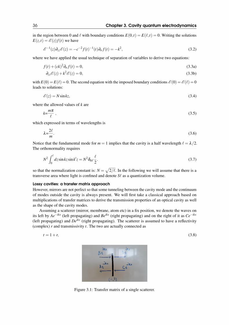
Lossy cavities: a transfer matrix approachHowever, mirrors are not perfect so that some tunneling between the cavity mode and the continuumof modes outside the cavity is always present. We will first take a classical approach based onmultiplications of transfer matrices to derive the transmission properties of an optical cavity as wellas the shape of the cavity modes.

Assuming a scatterer (mirror, membrane, atom etc) in a fix position, we denote the waves onits left by Ae−ikx (left propagating) and Beikx (right propagating) and on the right of it as Ce−ikx

(left propagating) and Deikx (right propagating). The scatterer is assumed to have a reflectivity(complex) r and transmissivity t. The two are actually connected as

t = 1+ r, (3.8)

Figure 3.1: Transfer matrix of a single scatterer.

3.1 Optical cavity - classical treatment 37

and notice that in the absence of absorption we have

|r|2 + |t|2 = 1. (3.9)

One can relate the outgoing fields to the incoming fields as

D = tB+ rC, (3.10a)

A = rB+ tD, (3.10b)

and rewrite the conditions connecting the amplitudes on the right side with the ones on the left sideof the beamsplitter:[

CD

]=

1t

[1 −rr t2− r2

][AB

]=

[1− iζ −iζ

iζ 1+ iζ

][AB

]. (3.11)

An important aspect is that the parametrization is done with a real polarizability ζ based on thefollowing transformation:

ζ =− irt=− ir

1− r. (3.12)

We can inverse this to obtain

r =−ζ

ζ − i. (3.13)

Notice that the intensity reflectivity is then given by

|r|2 = ζ 2

ζ 2 +1. (3.14)

which further allows to express

ζ2 =

|r|2

1−|r|2. (3.15)

For large polarizabilities one gets a close to unity reflectivity. Rewriting we get

r = |r|

[ζ√

1+ζ 2− i

1√1+ζ 2

]= |r|eiφ , (3.16)

with

sinφ =− 1√1+ζ 2

, and cosφ =ζ√

1+ζ 2. (3.17)

We can also inverse this transformation:[AB

]=

1t

[t2− r2 r−r 1

][CD

]. (3.18)

The free space accumulation of phase is easily written as[A′

B′

]=

[e−ik` 0

0 eik`

][AB

]. (3.19)


A two mirror arrangementLet’s now assume an arrangement of two identical mirrors at z = 0 and z = ` and no input from theright side (C = 0) while the left side has a unit propagating field amplitude (B = 1). We can thenwrite [

rc

1

]=

1t

[t2− r2 r−r 1

][e−ik` 0

0 eik`

]1t

[t2− r2 r−r 1

][0tc

], (3.20)

where now the D and A components become the transmission and reflection of the compound objecti.e. the optical cavity. With a bit of math one finds

1t2

[t2− r2 r−r 1

][e−ik` 0

0 eik`

][t2− r2 r−r 1

]= (3.21)

=1t2

[t2− r2 r−r 1

][e−ik`(t2− r2) re−ik`

−reik` eik`

]=

=1t2

[e−ik`(t2− r2)2 + r2eik` (t2− r2)re−ik`+ reik`

−(t2− r2)re−ik`− reik` −r2e−ik`+ eik`

].

Denoting the whole transfer matrix by M one can easily notice that

tc =1

M22=

t2

eik`− r2e−ik` =t2eik`

e2ik`− r2 . (3.22)

Let’s analyze the intensity transmission

Tc = |tc|2 =|t|2

|e2ik`− r2|2=

|t|2

|e2i(k`−φ)−|r|2|2=

|t|2

|e2i(k`−φ)−1+ |t|2|2. (3.23)

A maximum is possible at unity. Resonances are reached around the values we expected minus asmall contribution:

2km`= 2πm+2φ → km =πm`− φ

`. (3.24)

For large polarizability

φ '− 1√1+ζ 2

' ζ−1. (3.25)

Cavity linewidth, cavity decay rate and finesse.Expanding around the resonance condition:e−2ik` = 1− 2i(δk)` = 1− 2i(k− km), we obtain aLorentzian shape of the transmission function around some resonance km,

T mc (k) =

1|1+2iζ 2`(k− km)|2

. (3.26)

Notice that t =−i/ζ so that The linewidth of this Lorentzian is given by the condition of T mc (km +

δk) = 1/2 which leads to

δk =1

2ζ 2`. (3.27)

Expressed as a cavity decay rate (for units of frequency) one can define

κ = cδk =c

2ζ 2`. (3.28)

3.2 Optical cavity: quantum Langevin equations 39

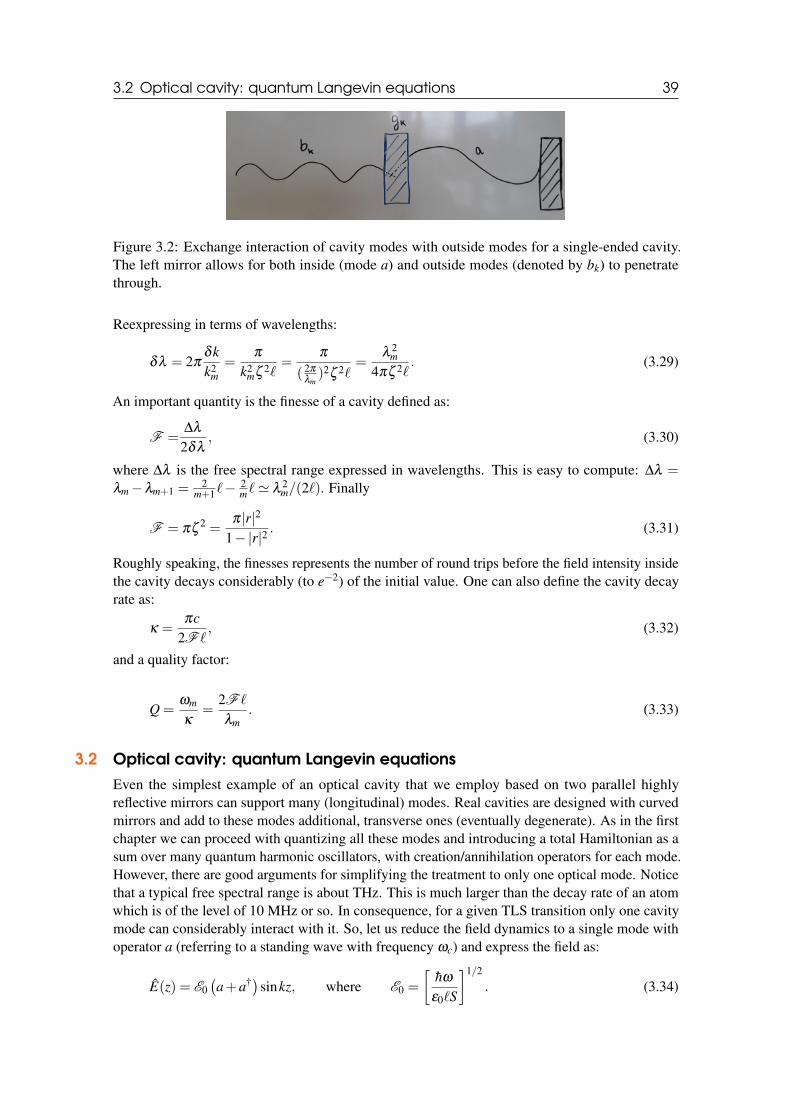
Figure 3.2: Exchange interaction of cavity modes with outside modes for a single-ended cavity.The left mirror allows for both inside (mode a) and outside modes (denoted by bk) to penetratethrough.

Reexpressing in terms of wavelengths:

δλ = 2πδkk2

m=

π

k2mζ 2`

=π

( 2π

λm)2ζ 2`

=λ 2

m

4πζ 2`. (3.29)

An important quantity is the finesse of a cavity defined as:

F =∆λ

2δλ, (3.30)

where ∆λ is the free spectral range expressed in wavelengths. This is easy to compute: ∆λ =λm−λm+1 =

2m+1`−

2m`' λ 2

m/(2`). Finally

F = πζ2 =

π|r|2

1−|r|2. (3.31)

Roughly speaking, the finesses represents the number of round trips before the field intensity insidethe cavity decays considerably (to e−2) of the initial value. One can also define the cavity decayrate as:

κ =πc

2F `, (3.32)

and a quality factor:

Q =ωm

κ=

2F `

λm. (3.33)

3.2 Optical cavity: quantum Langevin equationsEven the simplest example of an optical cavity that we employ based on two parallel highlyreflective mirrors can support many (longitudinal) modes. Real cavities are designed with curvedmirrors and add to these modes additional, transverse ones (eventually degenerate). As in the firstchapter we can proceed with quantizing all these modes and introducing a total Hamiltonian as asum over many quantum harmonic oscillators, with creation/annihilation operators for each mode.However, there are good arguments for simplifying the treatment to only one optical mode. Noticethat a typical free spectral range is about THz. This is much larger than the decay rate of an atomwhich is of the level of 10 MHz or so. In consequence, for a given TLS transition only one cavitymode can considerably interact with it. So, let us reduce the field dynamics to a single mode withoperator a (referring to a standing wave with frequency ωc) and express the field as:

E(z) = E0(a+a†)sinkz, where E0 =

[hω

ε0`S

]1/2

. (3.34)


We have introduced the mode area S and grouped terms inside the zero point electric field amplitudesuch that the integration of the Hamiltonian volume density over the whole volume leads to

H = hωc

[a†a+

12

]. (3.35)

As before we will disregard the constant energy shift. As the cavity mirrors are not perfect theintra-cavity field can permeate through the dielectric material and tunnel to the outside. At thesame time the outside field can also tunnel inside the cavity. If this were not the case than the cavitywould be useless as no driving would be possible. Having learned what the classical treatmentpredicts for a cavity resonance transmission linewidth, we are in the position of writing a quantummodel for the coupling of a quantized cavity mode to the continuum of modes outside. To thisend we consider the Hamiltonian for the cavity mode plus the infinity of outside modes and theirinteraction (modelled a an excitation exchange term)

H = hωca†a+∑k

hωkb†kbk + h∑

kgk

[b†

ka+a†bk

]. (3.36)

From here we can derive a set of equations of motion Let’s write the equations of motion:

a =ih[H,a] =−iωca− i∑

kgkbk, (3.37a)

bk =ih[H,bk] =−iωkbk− igka. (3.37b)

The plan is to formally integrate the equation of motion for the outside modes and plug the solutionsback into the cavity mode evolution equation. This will result in a differential-integro equation. Ina first step we have

bk(t) = bk(0)e−iωkt − igk

t∫0

dt ′a(t ′)e−iωk(t−t ′). (3.38)

Replacing this expression into the cavity mode equation of motion we obtain:

a =−iωca−∑k

g2k

t∫0

dt ′a(t ′)e−iωk(t−t ′)− i∑k

gkbk(0)e−iωkt . (3.39)

The decay rateThe first term, similarly to the summation performed in the case of the spontaneous emission masterequation for atoms, gives a delta function selecting only the coupling terms at the cavity frequency.The terms turns into a decay term

−∑k

g2k

t∫0

dt ′a(t ′)e−iωk(t−t ′) =−κa(t), (3.40)

at a rate which one can prove is the classically derived term in the previous section.

The input noiseThe second term is an infinite sum over the input modes which we will denote by

F(t) =−i∑k

gkbk(0)ei−ωkt . (3.41)

3.2 Optical cavity: quantum Langevin equations 41

Going back in the original picture we can write a Langevin equation:

a =−iωca(t)−κa(t)+F(t). (3.42)

Notice that in the vacuum

〈0|F(t)|0〉=−i∑k

gk〈0|bk(0)|0〉e−iωkt = 0. (3.43)

Looking at the correlations of the input term assuming the modes outside in the vacuum, all but oneterm vanish:

〈0|F(t)F†(t ′)|0〉= ∑k

g2ke−iωk(t−t ′) = 2κδ (t− t ′). (3.44)

Finally we can write a standard Langevin equation for the cavity mode under the following form:

a =−iωca(t)−κa(t)+√

2κAin, (3.45a)√

2κAin(t) = η +√

2κain(t), (3.45b)

For vacuum states the input noise is delta normalized such that 〈Ain(t)A†in(t′)〉= δ (t− t ′).

The driving termLet’s now assume that one of the incoming modes at frequency ckLis populated by a coherent stateαLwhile all the other modes are in the vacuum. We can then evaluate

〈αL|F(t)|αL〉=−i∑k

gk〈αL|bk(0)|αL〉eiωkt =−iαLe−iωLt . (3.46)

We then separate the input noise into a classical part and a zero-average quantum part:

F(t) =√

2κAin =−iαLe−iωLt +√

2κain. (3.47)

Generally, in terms of zero-average noise and classical drive, in a rotating frame at the laserfrequency one can write the following Langevin equation:

a =−κa− i(ωL−ωc)a+η +√

2κain , (3.48)

where we made the notation η =−iαL.

Input-output relationsSimilarly with the procedure above we can integrate the equation for the outside modes fromt to infinity.

bk(t) = bk(∞)+ i∞∫

t

dt ′gka(t ′)e−i(ω−ωk)t ′ . (3.49)

A similar calculation leads to

a =−iωca(t)+κa(t)−√

2κaout , (3.50)

where aoutstems from the new noise term

F(t) = i∑k

gkbk(∞)ei(ωc−ωk)t . (3.51)

This is a convoluted way of assuming that for an interaction that lasts for a limited time, the initialconditions are obtained by evaluating the fields outside at time 0 (or equivalently −∞) while thefinal state is obtained by evaluating the fields after the interaction at t = ∞. Finally we get the inputoutput relations:

Aout +Ain =√

2κa . (3.52)


Two sided cavities. Transmission and reflection.The input-output relations are valid at each interface. Let us assume a two-sided cavity with equalreflectivities and thus equal decay rates on each mirror κ/2. Driving occurs from the left and isincluded in the Ain term such that 〈Ain〉= η/

√κ . The input field (in zero average state) from the

right is denoted by bin. We then have:

Ain +Bout =√

κa, (3.53a)

bin +Aout =√

κa. (3.53b)

We can define transmission and reflection coefficients as: tc = 〈Aout〉/〈Ain〉and rc = 〈Bout〉/〈Ain〉.Taking an average over the equations above we have

1+ rc =κ

η〈a〉, (3.54a)

tc =κ

η〈a〉, (3.54b)

which gives the usual relation as we used in the transfer matrix tc = rc +1.The Langevin equationswith both input noises are:

a =−κa− i(ωL−ωc)a+η +√

κain +√

κbin, (3.55)

and a classical average in steady state (assuming times longer than κ−1) gives:

〈a〉= η

κ + i(ωL−ωc). (3.56)

Consequently the transmission of intensity is given by:

Tc = |tc|2 =κ2

κ2 +(ωL−ωc)2 . (3.57)

3.3 Optical cavity: master equation

Following the lines of the derivation carried out for spontaneous emission, we can show that thefollowing master equation for a driven cavity undergoing decay can be obtained:

ddt

ρ =− ih[H,ρ]+κ

aρa†− 1

2[a†aρ +ρa†a

], (3.58)

with

H = hωca†a+ ihη(aeiωLt −a†e−iωLt) . (3.59)

3.4 The Jaynes-Cummings Hamiltonian.

Let’s now place an atom within the cavity. We assume that the atom is closely resonant with agiven cavity resonance and far away from any other resonances. The dipole-electric field couplingHamiltonian will now be written as:

HJC = hg[a†

σ +aσ†] . (3.60)

3.4 The Jaynes-Cummings Hamiltonian. 43

The coupling strength is the usual:

g =1hE0deg =

[ω

hε0`S

]1/2

deg. (3.61)

Let us inspect the properties of a coupled atom-cavity field system without any incoherentprocesses. The full Hamiltonian is:

H = hωca†a+ hωaσ†σ + hg

[a†

σ +aσ†] . (3.62)

Let’s consider the complete basis in the full Hilbert space spanned by |g,n〉 and |e,n〉. All thepossible matrix elements are:

〈g,n|H|g,m〉= hωcnδnm, (3.63a)

〈e,n|H|e,m〉= hωcnδnm + hωaδnm, (3.63b)

〈g,n|H|e,m〉= hg√

n+1δnm+1, (3.63c)

〈e,n|H|g,m〉= hg√

nδnm−1. (3.63d)

Let’s write it in matrix form agreeing that we start with vectors ordered as: |g,0〉, |g,1〉, |e,0〉, |g,2〉,|e,1〉 ....

h

ωc +ωa g

√2 0 0 0

g√

2 2ωc 0 0 00 0 ωa g 00 0 g ωc 00 0 0 0 0

. (3.64)

Notice that for a given n only states |g,n+1〉and |e,n〉are coupled. One can then block diagonalizethe whole Hamiltonian in excitation subspaces spanned by a constant number of excitations.

We see that the Hamiltonian matrix contains blocks which are not coupled. Let’s first focus inthe single excitation block with state vectors |g,1〉, |e,0〉. To bring this block into diagonal form wehave to diagonalize the following matrix:[

ωa gg ωc

]. (3.65)

Eigenvalues are given by the equation: (ωa−λ )(ωc−λ ) = g2. Let’s rewrite this as: (λ −ωc +ωc−ωa)(λ −ωc) = g2 and make notations ωc−ωa = ∆.Then we have to solve: x2 +∆x−g2 = 0leading to

λ = ωc−∆

2±

√(∆

2

)2

+g2 =ωc +ωa

2±

√(ωc−ωa

2

)2

+g2. (3.66)

For zero detuning ωc = ωa = ω the two eigenstates are located at

E (1) = h(ω±g) , (3.67)

in energy and are combinations

|p±〉=|e,0〉±, |g,1〉√

2. (3.68)

In higher excitation subspaces, the result is (by diagonalizing the blocks with n photons):

E (n) = h(ω±g

√n). (3.69)


The polariton transformationFor the resonant case, we will perform a transformation from the bare atom and cavity operators topolariton operators:

u =

√12(a+σ), (3.70a)

d =

√12(a−σ). (3.70b)

The inverse transformations:

a =

√12(u+d), (3.71a)

σ =

√12(u−d). (3.71b)

Notice that the application of the polariton operators to the vacuum creates the previously derivedstates:

u†|g,0〉=√

12(a† +σ

†)|g,0〉= |e,0〉+ |g,1〉√2

. (3.72)

The Hamiltonian contains terms as:

a†a =12(u† +d†)(u+d) =

12(u†u+d†d +u†d +d†u

), (3.73a)

σ†σ =

12(u†−d†)(u−d) =

12(u†u+d†d−u†d−d†u

), (3.73b)

σ†a =

12(u†−d†)(u+d) =

12(u†u−d†d +u†d−d†u

), (3.73c)

a†σ =

12(u† +d†)(u−d) =

12(u†u−d†d−u†d +d†u

). (3.73d)

Adding everything we immediately find what we expected which is that the Hamiltonian can bediagonalized via this transformation:

H = h(ω−g)d†d + h(ω +g)u†u. (3.74)

The strong coupling regimeIntroducing decay we see that the polariton transformation already diagonalizes the Lindblad term.Let’s apply the transformation above to the Lindblad terms:

Lγ = γ[2σρσ

†−(σ

†σρ−ρσ

†σ)], (3.75)

Lκ = κ[2aρa†−

(a†aρ−ρa†a

)], (3.76)

Working it out:

2σρσ† = (u−d)ρ(u†−d†) = uρu† +dρd†−uρd†−dρu†, (3.77a)

σ†σρ =

12(u†−d†)(u−d)ρ = u†uρ +d†dρ−u†dρ−d†uρ, (3.77b)

ρσ†σ =

12

ρ(u†−d†)(u−d) = ρu†u+ρd†d−ρu†d−ρd†u, (3.77c)

3.4 The Jaynes-Cummings Hamiltonian. 45

Also

2aρa† = (u+d)ρ(u† +d†) = uρu† +dρd† +uρd† +dρu†, (3.78a)

a†aρ =12(u† +d†)(u+d)ρ = u†uρ +d†dρ +u†dρ +d†uρ, (3.78b)

ρa†a =12

ρ(u† +d†)(u+d) = ρu†u+ρd†d +ρu†d +ρd†u. (3.78c)

Adding everything we find a simple result:

L [ρ] = L(γ+κ)/2[d,ρ]+L(γ+κ)/2[u,ρ], (3.79)

which states that the two polariton operators make up two equally decaying channels at rates(γ +κ)/2.

The Purcell effectLet’s first investigate such interactions in the regime where the cavity field is very quickly decayingκ γ . We also assume the atom being resonant to the cavity mode both at ω . We can go into arotating frame where both a and σ rotate at the ω frequency. Thus, we have to solve the dynamicsof a system with the following complete dynamics:

ddt

ρ =−ig[a†

σ +aσ†,ρ]+κD [a,ρ]+ γD [σ ,ρ]. (3.80)

Let’s look at the evolution of the field operator:

ddt

a =−κa− igσ +√

2κain. (3.81)

We can go into a rotating frame where both a and σ rotate at the ω frequency. Formal integrationwill lead to

a(t) = a(0)e−κt − igt∫

0

dt ′σ(t ′)e−κ(t−t ′)−κa− igσ +√

2κ

t∫0

dt ′ain(t ′)e−κ(t−t ′). (3.82)

The first term decays fast and will vanish for t κ−1. The second term we will integrate by parts:

1κ

t∫0

dt ′σ(t ′)[eκt ′]′=

1κ

σ(t ′)eκt ′ |t0−1κ

t∫0

dt ′σ ′(t ′)eκt ′ . (3.83)

Putting it together we get:

−igt∫

0

dt ′σ(t ′)e−κ(t−t ′) =− igκ

(σ(t)−σ(0)e−κt)+ ig

κ

t∫0

dt ′σ ′(t ′)e−κ(t−t ′). (3.84)

The transient term will vanish again in the same long time limit. The second term can be againintegrated by parts and slowly we get smaller and smaller terms containing κ−2, κ−3etc. We thenconclude that:

a(t)'− igκ

σ(t)+ ain. (3.85)


Now let’s replace the first term in the expression in the Lindblad term for the cavity field:

κ

aρa†− 1

2[aaρ +ρa†a

]=

g2

κ

σρσ

†− 12[σ†

σρ +ρσ†σ]

. (3.86)

We see that the cavity contributes to the decay of the atom with a rate g2/κ . The total decay rate ofthe atom will therefore be:

γ +g2

κ= γ(1+C), (3.87)

where we will denote the cooperativity parameter by

C =g2

γκ. (3.88)

Let us remember what all these parameters are:

g2 =

[ω

hε0`S

]d2

eg (3.89a)

γ =d2

egω3

3πc3hε0, (3.89b)

κ =πc

2F `. (3.89c)

Putting it all together:

C =ω

hε0`Sd2

eg3πc3hε0

d2egω3

2F `

πc=

6F c2

Sω2 . (3.90)

Also, replacing ω/c = k = 2π/λ we have 6c2/ω2 = 6λ 2/(4π2) so that

C = F3λ 2

2π2

S. (3.91)

One can then only improve this quantity by designing better mirrors and focusing down the cavitymode area to small values.

3.5 Optical bistability

We will now add decay into the problem at ratesγ for the atom and κ for the cavity field. We alsoassume a weak pump coming through the left mirror and analyze the transmission properties of thesystem. We can derive the equations of motion for the field and atomic operators:

ddt〈a〉=−κ〈a〉+ i∆〈a〉− ig〈σ〉+η , (3.92a)

ddt〈σ〉=−γ〈σ〉+ i∆〈σ〉+ ig〈a

(σ

†σ −σσ

†)〉. (3.92b)

We assumed atoms resonant to the cavity mode and the detuning is ∆ = ωL−ωc. The equations arenon-linear as the last term contains correlations between the field and the atom dipole. However,under the weak pumping condition: η κ , the cavity field in steady state will have much less

3.5 Optical bistability 47

than one photon and the atom will pretty much stay close to the ground state. We therefore replaceσ†σ −σσ† with −1 and analyze the set of linearized equations

ddt〈a〉=−κ〈a〉+ i∆〈a〉− ig〈σ〉+η , (3.93a)

ddt〈σ〉=−γ〈σ〉+ i∆〈σ〉− ig〈a〉. (3.93b)

Looking at steady state we have:

〈σ〉=− igγ− i∆

〈a〉, (3.94)

such that

〈a〉[

κ− i∆+g2

γ− i∆

]= η . (3.95)

Rewriting the last equation:

〈a〉[

κ +g2γ

γ2 +∆2 − i∆(

1− g2

γ2 +∆2

)]= η . (3.96)

Remember from last lecture that the transmission of the cavity is:

Tc =

∣∣∣∣√κ〈a〉η/√

κ

∣∣∣∣2 = κ2∣∣∣κ + g2γ

γ2+∆2 − i∆(

1− g2

γ2+∆2

)∣∣∣2 . (3.97)

One observation is that we see that ∆ = 0 gives the maximum so the minimum of the transmissionat

Tc(∆ = 0) =κ2∣∣∣κ + g2

γ

∣∣∣2 =1

(1+C)2 , (3.98)

where the cooperativity C = g2/(κγ) (just as before in the limit of bad-cavity we defined itproportional to the Purcell factor) plays a major role. One can also see the effect in the next orderapproximation for the equation of motion when more significant population in the excited state istaken into account. Let’s rewrite

ddt〈a〉=−κ〈a〉+ i∆〈a〉− ig〈σ〉+η , (3.99)

ddt〈σ〉=−γ〈σ〉+ i∆〈σ〉+ ig〈a

(σ

†σ −σσ

†)〉. (3.100)

ddt〈σ†

σ −σσ†〉=−2γ〈σ†

σ −σσ†〉+ ig〈a†

σ −aσ†〉−2γ. (3.101)

We perform two factorizations〈a(σ†σ −σσ†

)〉= 〈σ†σ−σσ†〉〈a〉 and 〈a†σ−aσ†〉= 〈a†〉〈σ〉−

〈a〉〈σ†〉 and evaluate in steady state:

〈σ〉(γ− i∆) = ig〈a〉〈σ†σ −σσ

†〉, (3.102)

〈σ〉∗ (γ + i∆) =−ig〈a〉∗〈σ†σ −σσ

†〉. (3.103)

This immediatily leads to

ig〈a〉∗〈σ〉(γ− i∆) =−g2|〈a〉|2〈σ†σ −σσ

†〉, (3.104)

−ig〈a〉〈σ〉∗ (γ + i∆) =−g2|〈a〉|2〈σ†σ −σσ

†〉, (3.105)


so that

ig〈a†σ −aσ

†〉=− 2γg2

γ2 +∆2 |〈a〉|2〈σ†

σ −σσ†〉 (3.106)

The equation for the population difference then gives

〈σ†σ −σσ

†〉=−1− 2g2

γ2 +∆2 |〈a〉|2〈σ†

σ −σσ†〉 → 〈σ†

σ −σσ†〉= −1

1+ 2g2

γ2+∆2 |〈a〉|2.

(3.107)

Now we directly have

〈σ〉= −igγ− i∆

〈a〉1+ 2g2

γ2+∆2 |〈a〉|2, (3.108)

which leads to the cavity field amplitude in steady state:

〈a〉(κ− i∆) =−g2

γ− i∆〈a〉

1+ 2g2

γ2+∆2 |〈a〉|2+η , (3.109)

or

〈a〉

(κ− i∆)+1

1+ 2g2

γ2+∆2 |〈a〉|2g2

γ− i∆

= η . (3.110)

The expression above shows that the cavity resonances are shifted for larger input fields as theintracavity field intensity depends nonlinearly on the input field. Taking the absolute value squaredfor the above expression leads to

Ic

∣∣∣∣∣∣(κ− i∆)+1

1+ 2g2

γ2+∆2 Ic

g2

γ− i∆

∣∣∣∣∣∣2

= Ip, (3.111)

which is an equation with more than one solution (three) for give ranges of the input For example,at ∆ = 0,

Icκ2

1+C2(

1+ 2g2

γ2 Ic

)2

= Ip, (3.112)

leading to

Icκ2

((1+

2g2

γ2 Ic

)2

+C2

)= Ip

(1+

2g2

γ2 Ic

)2

. (3.113)

3.6 Photon blockadeOne notices that in the first and second excitation manifolds nonlinearities appear due to theprogressive g

√n shifts of levels. Looking at the resonance condition for single cavity input photon

one notices two resonances at the lower (at ω−g ) and at the upper (ω +g) polaritons. Assumingthe driving frequency at the lower polariton, one can also notice that the 2 photon resonancecondition is not fulfilled as a detuning (2ω−

√2g)−2(ω−g) = (2−

√2)g appears. In the limit

that this detuning is very large, the presence of the atom strongly coupled to the cavity effectivelysuppresses the entering of a second photon, thus providing a photon blockade mechanism.

3.7 Appendix: Langevin equations in the Fourier domain. 49

3.7 Appendix: Langevin equations in the Fourier domain.A Fourier transformation can simplify our task of finding operator averages and correlations (atequal or different times) as it transforms the set of coupled differential equations into an ordinaryset of equations. Notice however that this is only valid around steady state. When one needs to takethe initial conditions into account, the Laplace transform can be used instead.

Let us introduce the Fourier transform of the time dependent operators:

a(ω) = F [a(t)] =1√2π

∫dta(t)e+iωt , (3.114)

a(t) =1√2π

∫dωa(ω)e−iωt . (3.115)

Notice two properties. First the Fourier transform of a derivative is:

F [a(t)] =−iωa(ω), (3.116)

Second, we use:

a†(ω) = F [a†(t)] =1√2π

∫dta†(t)e+iωt , (3.117)

which leads to:

[a(ω)]† =1√2π

∫dta†(t)e−iωt = a†(−ω). (3.118)

For delta-correlated input noise (of zero average) then we have:

〈a(ω)a†(ω ′)〉= 12π

∫dt∫

dt ′〈a(t)a†(t ′)〉e+iωte+iω ′t ′ = (3.119)

=1

2π

∫dt∫

dt ′δ (t− t ′)e+iωte+iω ′t ′ =1

2π

∫dte+i(ω+ω ′)t = δ (ω +ω

′). (3.120)

We consider a driven cavity

a =−κa+ i∆a+η +√

κ (ain +bin) , (3.121)

and first linearize around steady state:

δa =−κδa+ i∆δa+√

2κdin, (3.122)

while the average is as above. We also wrote din = (ain +bin)/√

2 with the combined input noisebeing delta correlated in time. Taking the Fourier transform:

δa(ω) [κ− i(∆+ω)] =√

2κdin(ω), (3.123)

together with its couterpart

δa†(ω) [κ + i(∆−ω)] =√

2κd†in(ω). (3.124)

One can express these in terms of the susceptibilities:

δa(ω) = ε(ω)√

2κdin(ω), (3.125)


δa†(ω) = ε∗(−ω)

√2κd†

in(ω), (3.126)

The intracavity correlations are:

〈δa(ω)δa†(ω ′)〉= ε(ω)ε∗(−ω′)2κ〈din(ω)d†

in(ω′)〉= (3.127)

= 2κ |ε(ω)|2 δ (ω +ω′) =

2κ

κ2 +(∆+ω)2 δ (ω +ω′). (3.128)

The linearized input-output relations (for zero-average operators) transform straighforwardly intothe Fourier space:

aout(ω) =√

κδa(ω)−bin(ω), (3.129)

bout(ω) =√

κδa(ω)−ain(ω), (3.130)

and

a†out(ω) =

√κδa†(ω)−b†

in(ω), (3.131)

b†out(ω) =

√κδa†(ω)−a†

in(ω). (3.132)

One can connect output noise to input noise directly:

aout(ω) = ε(ω)κain(ω)−bin(ω) [1− ε(ω)κ] , (3.133)

a†out(ω) = ε

∗(−ω)κa†in(ω)−b†

in(ω) [1− ε∗(−ω)κ] , (3.134)

Now we can express for example:

〈aout(ω)a†out(ω

′)〉= ε(ω)ε∗(−ω′)κ2〈ain(ω)a†

in(ω′)〉+[1− ε(ω)κ]

[1− ε

∗(−ω′)κ]〈bin(ω)b†

in(ω′)〉=

(3.135)

=[1+2κ

2|ε(ω)|2−2κRe[ε(ω)]]

δ (ω +ω′) = (3.136)

=

[1+

2κ2

κ2 +(∆+ω)2 −2κκ

κ2 +(∆+ω)2

]δ (ω +ω

′) = δ (ω +ω′) (3.137)

4. Fundamentals of laser theory

We will now make use of the techniques developed in the previous chapters to describe a fewcharacteristics of a lasing cavity filled with a gain medium. Our goals are modest as we onlyaim at providing a simplistic treatment to reveal two main characteristic of lasing action: i) theexistence of a threshold for lasing connected to the achieved population inversion, and ii) thestatistics of photons exiting a laser cavity (ideally close to a Poisson distribution characteristic of acoherent state). We will employ two slightly different models to derive these crucial aspects. First,we assume a collection of effective two level systems incoherently pumped such that populationinversion can be achieved. We show that in the macroscopic limit of large number of gain mediumatoms the cavity can sustain the build-up of a non-zero amplitude field past a certain pumpingthreshold. We then follow a standard approach (Milburn, Scully) of four-level systems passingthrough a cavity to arrive at a simplified form for the photon number distribution and prove thatpast the threhold a laser exhibits Poissonian statistics. Finally, we analyze the laser linewidth bywell above threshold and connect it to the diffusion process that the cavity field undergoes duringspontaneous emission events.

4.1 Laser thresholdWe assume N identical two level systems equally coupled to a cavity mode. The Hamiltonian of thesystem is comprised of

H0 = hωa†a+∑j

hωσ( j)z , (4.1a)

HJC = ∑j

hg[a†

σ j +aσ†j

]. (4.1b)

The Lindblad terms contain the natural spontaneous emission at rate γ , cavity decay at rate κ as wellas the engineered pump rate (described as an artificial inverse decay terms as derived in Chapter 2)at rate Γ

L = γ ∑j

D [σ j,ρ]+Γ∑j

D [σ†j ,ρ]+κ ∑

jD [a,ρ]. (4.2)

52 Chapter 4. Fundamentals of laser theory

Of course we can immediately get rid of the free evolution by moving into the interaction picturewith respect to H0. We can write equations of motion for the averages:

ddt〈a〉=−κ〈a〉− ig∑

j〈σ j〉, (4.3a)

ddt〈σ j〉=−

Γ+ γ

2〈σ j〉+2ig〈aσ

( j)z 〉, (4.3b)

ddt〈σ ( j)

z 〉=−(Γ+ γ)〈σ ( j)z 〉+ ig〈a†

σ j−aσ†j 〉+

Γ− γ

2. (4.3c)

Let’s quickly check that this is correct. In the absence of coupling to the cavity starting with theground state we get a steady state with

〈σ ( j)z 〉=

Γ− γ

2(Γ+ γ)= d0. (4.4)

This is the expected population inversion when pumping the system. If Γ γ , we get d0 close to1/2 meaning most of the population is in the excited state. The above equations are coupled andnonlinear and thus not easy to solve. First we notice that we can perform sums such that:

ddt〈a〉=−κ〈a〉− ig〈S〉, (4.5a)

ddt〈S〉=−Γ+ γ

2〈S〉+2ig〈aSz〉, (4.5b)

ddt〈Sz〉=−(Γ+ γ)〈Sz〉+ ig〈a†S−aS†〉+N

Γ− γ

2. (4.5c)

where the collective operators are:

S = ∑j

σ j and Sz = ∑j

σ( j)z . (4.6)

In steady state without cavity we will now have 〈Sz〉= Nd0 = D0.In the large system expansionwhen N 1, one can analyze the classical equations for this system by factorizing (we split eachoperator into an average and a zero average fluctuation):

〈aSz〉= 〈(α +δa)(sz +δSz)〉= αsz + 〈δaδSz〉 ' αsz, (4.7a)

〈a†S〉= 〈(α∗+δa†)(s+δS)〉= α

∗s+ 〈δa†δS〉 ' α

∗s, (4.7b)

〈aS†〉= 〈(α +δa)(s∗+δS†)〉= αs∗+ 〈δaδS†〉 ' αs∗. (4.7c)

This should be valid as long as the averages of fluctuation products are small compared to theaverages.

Classical equations. Threshold.Let’s proceed with the system to be solved:

dα

dt=−κα− igs, (4.8a)

dsdt

=−Γ+ γ

2s+2igαsz, (4.8b)

dsz

dt=−(Γ+ γ)sz + ig(α∗s−αs∗)+N

Γ− γ

2. (4.8c)

4.1 Laser threshold 53

We set steady state conditions and notice that

s =4ig

Γ+ γαsz. (4.9)

Replacing in equation 3 we get:[(Γ+ γ)+

8g2

Γ+ γ|α|2

]sz = N

Γ− γ

2. (4.10)

In simplified notation:

sz =D0

1+ 8g2

(Γ+γ)2 |α|2. (4.11)

Notice that as the cavity field is turned on the population inversion starts going down. We can nowcompute:

s =4ig

Γ+ γ

D0

1+ 8g2

(Γ+γ)2 |α|2α, (4.12)

which leads to an effective equation of motion for the cavity field amplitude:

dα

dt=−κα +

4g2

Γ+ γ

D0

1+ 8g2

(Γ+γ)2 |α|2α. (4.13)

With more notations:

n0 =(Γ+ γ)2

8g2 , C =4g2D0

κ(Γ+ γ)=

2g2 (Γ− γ)

κ(Γ+ γ)2 '2g2

κΓ(4.14)

we can rewrite:

dα

dt= κ

[−1+

C1+ |α|2/n0

]α. (4.15)

It is easy to see that the steady state is zero unless the gain surpasses the cavity loss. We then find athresold at C = 1 and compute the cavity field intensity as:

1 =C

1+ |α|2/n0, leading to |α|2 = n0 (C−1) . (4.16)

Well above thresholdConsider C 1 and look again at the population inversion

sz =D0

C=

κΓ

4g2,=

Γ2

8g2κ

Γ. (4.17)

Notice that as the cavity field is turned on the population inversion starts going down. We can nowcompute:

s =4ig

Γ+ γ

D0

1+ 8g2

(Γ+γ)2 |α|2α, (4.18)


4.2 Photon statistics of a laserWe now move to a more standard model for deriving equations for the reduced density operator ofthe cavity field alone. The goal is to find the photon number distribution of cavity photons belowand above threshold and see the transition from thermal light to coherent light in the cavity output.The model is used extensively in Quantum Optics textbooks (Milburn, Scully, etc). It consists ofa collection of four level atoms where the important ones are levels |2〉 (excited) and |1〉(ground)both of them decaying to some other levels with γ2 (from |2〉to |4〉) and with γ1(from |1〉to |3〉).There is no spontaneous emission (or negligible) between the lasing levels, and the transition iscoupled resonantly to a cavity field.

Model assumptionsThe atoms are prepared in the excited state and sent through the cavity spending a time τ insidewhich is much larger than the time it takes the atoms to reach steady state (roughly given by γ

−11,2 ).

The rate of which atoms are pushed into the cavity is r (understood as number of atoms per unittime). The probability of an atom entering the cavity during a small time interval ∆t would then ber∆t while the opposite event has the probability (1− r∆t). We now assume that at time t the cavityfield is in state ρ(t). After the passing of an atom through the cavity the reduced cavity field densityoperator becomes

ρF(t +∆t) = P(∆t)ρF(t). (4.19)

Summing together probabilities that either an atom passed or not through the cavity we will have afinal density operator for the cavity:

ρF(t +∆t) = r∆tP(∆t)ρF(t)+(1− r∆t)ρF(t). (4.20)

In the small ∆t limit, we will have an effective reduced master equation:

dρF(t)dt

= r(P−1)ρF(t)+κDa[ρF ], (4.21)

after writing the difference as a derivative and adding the decay Lindblad term for the cavity field.

The action of a single atom on the cavity fieldLet us now focus on deriving the action P(∆t). We set the initial time to zero for simplicity andconsider an initial density matrix generally expressed as:

ρF =∞

∑n,m=0

ρFnm(0)|n〉〈m|. (4.22)

Of course the atom initial density matrix is |2〉〈2|. We will show that

ρF(∆t) =∞

∑n,m=0

ρFnm(0) [Anm|n〉〈m|+Bnm|n+1〉〈m+1|] . (4.23)

The master equation to be solved during the ∆t time interval evolution is:

dρ(t)dt

=ih[H,ρ]+ γDσ1 [ρ]+ γDσ2 [ρ], (4.24)

where σ1 = |3〉〈1| and σ2 = |4〉〈2| and the D superoperators acts as usual as Lindblad termsdescribing decay. Notice that one can rewrite the master equation in the following form:

dρ(t)dt

=ih

[He f f ρ−ρH†

e f f

]+R[ρ], (4.25)


grouping recycling terms:

R[ρ] = 2γ

[σ1ρσ

†1 +σ2ρσ

†2

], (4.26)

and adding the rest in an effective Hamiltonian (careful that this is an effective non-hermitianevolution operator)

He f f = H− iγ(

σ†1 σ1 +σ

†2 σ2

). (4.27)

A zeroth order solution can be found by taking the derivatives of the following function:

ρ0(t) = B(t)ρ(0)B†(t) = S(t)[ρ(0)], (4.28)

satisfying the equation:

dρ0(t)dt

=ih

[He f f ρ0(t)−ρ0(t)H

†e f f

]. (4.29)

Now we look for the next order solution of the form:

ρ(t) = ρ0(t)+B(t) [ρ1(t)]B†(t) = S(t)[ρ(0)]+S(t)[ρ1(t)]. (4.30)

One can check that the master equation turns into:

dρ0(t)dt

+ B(t) [ρ1(t)]B†(t)+ B(t) [ρ1(t)]B†(t)+ B(t) [ρ1(t)] B†(t) = (4.31)

=ih

[He f f ρ0−ρ0H†

e f f

]+

ih

[He f f B(t) [ρ1(t)]B†(t)−B(t) [ρ1(t)]B†(t)H†

e f f

]+

R[ρ0 +B(t) [R[ρ1(t)]]B†(t).

After simplifications one arrives at (ignoring the last term):

dρ1(t)dt

= B(t) [R[ρ0(t)]]B†(t) = S(t) [R [S(t) [ρ(0)]]] , (4.32)

and integration gives:

ρ1(∆t) =∆t∫

0

dtS(t) [R [S(t) [ρ(0)]]] . (4.33)

Finally, one can put it all together:

ρ(∆t) = S(∆t) [ρ(0)]+∆t∫

0

dtS(t) [R [S(t) [ρ(0)]]]+ .... (4.34)

After painful calculations one can derive the next order terms and show that they are vanishing.Let’s therefore focus on the zeroth and first order term. We are left with evaluating terms like:

B(∆t)|n〉|2〉= c+n (∆t)|n,+〉+ c−n (∆t)|n,−〉, (4.35)

where the states defined as

|n±〉=1√2[|n,2〉± |n,1〉] (4.36)


are the polariton states in the n+1 excitation manifold. One can find a simple expression (based onthe assumptions γ1 = γ2):

c+n (∆t) =1

2√

2e−ig

√n+1te−γ∆t , (4.37a)

c−n (∆t) =1

2√

2eig√

n+1te−γ∆t . (4.37b)

We can find the first action:

S(t)[ρ(0)] = B(t)ρ(0)B†(t) =[c+n (t)|n+〉+ c−n (t)|n−〉

][c+∗n (t)〈n+|+ c−∗n (t)〈n−|

]. (4.38)

When plugged in to replace the zeroth order solution the results is zero in the limit ∆t γ−1. Thenext term however will not vanish. Let’s first calculate one term to get an idea what the recyclingterm does.

R [|n+〉〈n+|] = 2γ

[σ1|n+〉〈n+|σ†

1 +σ2|n+〉〈n+|σ†2

]= (4.39)

= γ [|n+1,3〉〈n+1,3|+ |n,4〉〈n,4|] .

Then we can work out all the other terms and trace over the atomic states to obtain:

TrA [S(t) [R [S(t) [ρ(0)]]]] = γ[c+n (t)+ c−n (t)

][c+∗m (t)+ c−∗m (t)

]|n〉〈m|+ (4.40)

+ γ[c+n (t)− c−n (t)

][c+∗m (t)− c−∗m (t)

]|n+1〉〈m+1|.

Finally, performing the integral over the first order solution one obtaines:

ρF(∆t) =∞

∑n,m=0

ρFnm(0) [Anm|n〉〈m|+Bnm|n+1〉〈m+1|] , (4.41)

where

Anm =

∆t∫0

dt[c+n (t)+ c−n (t)

][c+∗m (t)+ c−∗m (t)

], (4.42a)

Bnm =

∆t∫0

dt[c+n (t)− c−n (t)

][c+∗m (t)− c−∗m (t)

]. (4.42b)

For the diagonal elements one can check that the result is:

Ann =g2(n+1)+2γ2

2g2(n+1)+ γ2 , (4.43a)

Bnn = 1−Ann. (4.43b)

The reduced master equation and photon statisticsPutting together the results of the last two subsections we get an effective master equations writtenas:

dρnm

dt= G

[ √nm

1+(n+m)/(2ns)ρn−1,m−1−

(m+n+2)/2+(m−n)2/(8ns)

1+(n+m+2)/(2ns)ρnm

]+ (4.44)

+κ

[2√(n+1)(m+1)ρn+1,m+1− (n+m)ρnm

].


The gain is derived as:

G =r

2ns, where ns =

γ2

g2 . (4.45)

Focusing now on the photon number distribution, let’s consider the diagonal elements (pn = ρnn):

d pn

dt=−G

[n+1

1+(n+1)/nspn−

n1+n/ns

pn−1

]+2κ [(n+1)pn+1−κnpn] . (4.46)

We will analyze some simplified cases.

Thermal statistics (below threshold)The first one assumes ns 1 such that the average photon number is much smaller than ns. Thisallows the approximation leading to:

d pn

dt=−G [(n+1)pn−npn−1]+2κ [(n+1)pn+1−κnpn] . (4.47)

In steady state one can show that the solution to this recursive equation is:

pn = p0

(G2κ

)n

. (4.48)

Together with the normalization condition ∑ pn = 1, one can deduce

pn =

(1− G

2κ

)−1( G2κ

)n

. (4.49)

This can be casted in terms of a black-body radiation distribution with the identification:

G2κ

= e−hω

kBT , (4.50)

where one computes the effective temperature for values lower than the threshold. Notice that theaverage number of photons in the cavity (in thermal state) is

n =G

2κ−G. (4.51)

As a remark, the amplitude of the field is zero; characteristically of the thermal state, the averagephoton number instead is non-zero and equal to the fluctuations.

Poisson statistics (well-above threshold)We now assume that we are well beyond threshold such that n ns and only look at photonnumbers around the average (since we expect a Poisson distribution quite narrow far from thethreshold). We can approximate again:

d pn

dt=−G [ns pn−ns pn−1]+2κ [(n+1)pn+1−κnpn] . (4.52)

Setting steady state condition, the recursive equation leads to the following solution:

pn = e−n nn

n!, (4.53)

with an average photon number

n =Gns

2κ. (4.54)

This is a Poisson distribution made up by the contribution of many coherent states with differentphases.


Four-level system: Laser linewidth.The phase of the output light is undergoing a continuous phase diffusion owing to the spontaneousemission events accompanying the coherent exchanges between excited atoms and the cavity field.While the Poisson nature indicates that the amplitude of the cavity field stays pretty much stable,we can derive an equation for the damping of the phase. Let’s first write:

〈a〉= Tr [aρF ] =∞

∑n=0〈n|aρF |n〉=

∞

∑n=1

√nρn,n−1. (4.55)

and its derivative

ddt〈a〉=

∞

∑n=1

√n

ddt

ρn,n−1. (4.56)

Using the general equation derived above for the laser, one can show (see Scully) that:

ddt〈a〉=−G

2

∞

∑n=1

1/(4ns)−11+(2n+1)/(2ns)

ρn,n−1 '−G8n〈a〉. (4.57)

We can also look at the laser field spectrum defined as (and using a quantum regression theorem):

S(ω) =1√2π

∫dτ〈a†(τ)a(0)〉e−iωτ = F [ne−

G8nτ ] =

n

ω2 +( G

8n

)2 . (4.58)

The conclusion is that the laser spectrum is a Lorentzian with a linewidth of

∆ω =G8n

. (4.59)

5. Cooling of atoms

Up to here we examined fundamental processes between quantized light (photons) and static two(or more than two) level systems. However, as a photon is emitted or absorbed by an atom a transferof momentum occurs modifying its initial motional state. In order to properly account for this wewill supplement the starting Hamiltonian of a TLS in a box containing quantized light with the freeparticle Hamiltonian. This allows us then to derive the effect of stimulated absorption/emissionas well as that of spontaneous emission on the atom. The fact that light can have an impact onthe motion of atoms also means that manipulation of its state means of lasers is possible. In asemiclassical approximation we then exemplify a simple derivation of the cooling force of a TLSin plane and standing waves. This is known as Doppler cooling. We describe its particularitiesincluding the final achievable temperature. We also shortly review dipole forces (arising frommotion in focused light beams used in optical tweezers) and describe the mechanism for polarizationgradient cooling.

5.1 Light-induced forces.

Let us consider an atom moving in one dimension only (axis y) and quantize its motion (that ofthe nucleus) by imposing the commutation relations [y, p] = ih. In the absence of any confiningpotentials or interaction its evolution is described by the kinetic energy operator p2/2M. Onecan go either in the position or momentum representation to describe the system’s evolution. Wechoose (for a good reason) the momentum representation where the basis is given by |p〉 such thatp |p〉= p |p〉 and p |p〉= ih∂p |p〉. Notice that in this reciprocal space representation the action thefollowing action is simply a translation (the proof involves a Taylor expansion)

eiky |p〉= |p+ hk〉 . (5.1)

Of course the atom, as it has an internal electronic structure will also have the following freeHamiltonian hωσ†σ . The basis for the Hilbert space just increased as it contains |g, p〉 or |e, p〉.On top of this the atom is always in contact with the electromagnetic environment. We also assumea laser drive, which after the Mollow transformation (presented in the first chapter) is included as a

60 Chapter 5. Cooling of atoms

Figure 5.1: An atom is assumed to move in one (quantized) direction y and can be driven withz-polarized fields. The laser drive is in the positive y direction with momentum k0. Photons can bespontaneously emitted in all directions meaning that the recoil kicks suffered by the atom can be inany direction. However, we only quantify the mechanical effect in the direction of interest.

semiclassical term. We fix the direction and magnitude of the laser drive as k0εy, Rabi frequencyΩ` and its frequency ω`. Let’s write the total Hamiltonian:

H =p2

2M+ hω0σ

†σ +∑

khωka†

kak + hΩ`

(σeiω`te−ik0y +σ

†e−iω`teik0y)

(5.2)

+∑k

hgk

(σa†

ke−ikyye−i(kxx+kzz)+akσ†eikyyei(kxx+kzz)

)Notice that as we only quantized the motion along the y-axis we write the other two coordinateswithout a hat. Also we have assumed that the electronic transition can be excited only by a z-polarized light field. The total Hilbert space now spans all the momentum states, the ground orexcited for internal electronic states and all the states of the photon field with occupancies from 0to infinity. However the interesting states are limited to initial states of the form: |p0〉⊗ |g〉⊗ |0〉or |p0〉⊗ |e〉⊗ |0〉. We basically reproduce the derivation of fundamental light-matter scatteringprocesses described in the first chapter but considering now the change in the particle’s motion.First we take the atom in the ground state and compute the final possible states:

H |p0〉⊗ |g〉⊗ |0〉=p2

02M|p0〉⊗ |g〉⊗ |0〉+ hΩè−iω`t |p0− hk0〉⊗ |e〉⊗ |0〉 (5.3)

We have just deduced that the stimulated absorption process is actually accompanied by a changeof the state of the atom by the photon transferred momentum. Notice that, as expected, the vacuumstates do not play a role in this process. However, when starting in the excited state we will have adifferent expression:

H |p0〉⊗ |e〉⊗ |0〉=(

p20

2M+ hω0

)|p0〉⊗ |g〉⊗ |0〉+ hΩèiω`t |p0 + hk0〉⊗ |g〉⊗ |0〉 (5.4)

+∑k

hgke−ikyye−i(kxx+kzz) |p0− hky〉⊗ |g〉⊗ |0〉 .

The above expression includes terms associated with the stimulated emission showing a change inthe momentum by hk0 (opposite in sign to the change acquired with stimulated absorption) andchanges in momentum with the projection on the y-axis of the momentum of the spontaneouslyemitted photon hky. Let us now proceed by deriving a fully quantum expression for the force acting

5.2 Doppler cooling 61

onto the atom by making use of the Heisenberg equations of motion:

∂t p =iΩ`

(σeiω`t [e−ik0y, p]+σ

†e−iω`t [eik0y, p])

(5.5)

+∑k

igk

(σa†

k[e−ikyy, p]e−i(kxx+kzz)+akσ

†[eikyy, p]ei(kxx+kzz)).

We see that we need to evaluate commutators like [e±iky, p]. This we can do by expanding theexponential

[eiky, p] =∞

∑j=0

(ik) j

j![y j, p] = 0+

(ik)1

1!(ih)+

(ik)2

2!2ihy+

(ik)3

3!3ihy2 + ...=−hkeiky. (5.6)

Above we have used the general rule that [y j, p] = [yy j−1, p] = y[y j−1, p]+ [y, p]y j−1. For the signchange in the exponential we obtain a simple sign change in the momentum: [e−iky, p] = hkeiky.Finally we can properly write the equation of motion.

∂t p =ihk0Ω`

(σeiω`te−ik0y−σ

†e−iω`teik0y)

(5.7)

+∑k

ihkygk

(σa†

ke−ikyye−i(kxx+kzz)−akσ†eikyyei(kxx+kzz)

).

We obtain two contributions, one from the laser drive and a second one from the vacuum field.

5.2 Doppler cooling

Any light emission or absorption event by an atom is associated with a transfer of momentum∆p = hk = hω/c. If absorption is followed by stimulated emission then the momentum change atabsorption will cancel the momentum change at emission and no net momentum is transfered tothe atom. If absorption is followed by spontaneous emission, as the spontaneously emitted atom,on average a net momentum change will be obtained. Assuming an atom initially at rest, the recoilenergy can be computed from the acquired kinetic energy (∆p)2/2m. One can then define a recoilfrequency:

hωrec =(∆p)2

2m=

(hk)2

2m. (5.8)

For atoms, the value is typically in the range of kHz. To derive the effect of a light field ontothe motion of an atom we will first consider a semiclassical formulation where the atom positionand momentum are classical parameters undergoing some trajectory described by R(t) and P(t).We will the write a Hamiltonian that has these variables as parameters (so it is a time dependentHamiltonian):

HA+F = HA +HV +HA−L +HA−V , (5.9)

separated into free atom Hamiltonian and free vacuum field Hamiltonian,

HA +HV = hωegσ†σ +∑

khωka†

kak. (5.10)

classical laser-atom interaction (already in the rotating wave approximation)

HA+L = h[Ω(R)σeiωLt +Ω

∗(R)σ†e−iωLt] , (5.11)


and quantum vacuum field-atom interaction (also already in the rotating wave approximation)

HA+V = h∑k(gka†

kσe−ik·R +g∗kakσ†eik·R). (5.12)

We can derive a semiclassical force operator:

F(R) =−〈∇H〉=−〈∇HA−L〉−〈∇HA−V 〉, (5.13)

stemming from the effect of the laser onto the atom and of the vacuum onto the atom as well. Thevacuum force is a zero average force as one can derive from applying the gradient: ∇eik·R = keik·Randsumming over alll directions. Let us analyze the laser driving induced force which is

−〈∇HA−L〉=−h [∇Ω(R)]〈σ〉eiωLt − h [∇Ω∗(R)]〈σ†〉e−iωLt . (5.14)

The averages that we have to compute are simply the density matrix elements ρeg,ρge (coherences)in the fast rotating frame. We can reexpress

F(R) =−2hℜ[∇Ω(R)ρegeiωLt] . (5.15)

Let us assume that the atom is driven by a plane wave with k = kz propagating from left to right.The electric field assumed polarized in the x direction is a sum of positive and negative frequencyterms: a plane wave with the electric field:

E(R, t) = E(+)(R, t)+E(−)(R, t) = E0e−iωLteik·Rx+E0eiωLte−ik·Rx = (5.16)

= 2E0xcos(k ·R−ωLt) = 2E0 cos(kz−ωLt). (5.17)

We aim at computing the semiclassical force expression from the expression above with Ω(R)replaced by Ωeikz. We immediatily see that

F(z) =−2hkΩℜ

[ρegeikzeiωLt

]z (5.18)

5.2.1 Modified Bloch equationsWe have previously derived a set of Bloch equations for static atoms. Now the driving Hamiltonianhas a position dependence on theR function:

HA+L = hΩ

[σe−ikzeiωLt +σ

†eikze−iωLt], (5.19)

It is easy to compute the modified Bloch equations in the original frame (making no transformationsyet)

ddt

ρee =−γρee− iΩ[e−iωLteikz

ρge− eiωLte−ikzρeg

], (5.20)

ddt

ρeg =−γ

2ρeg− iωegρeg + iΩeikze−iωLt (ρgg−ρee) . (5.21)

We see that in order to eliminate the time dependence we will have to transform to a slow movingframe by removing the laser frequency: ρeg = ρege−iωLt . With∆ = ωeg−ωL we have

ddt

ρee =−γρee− iΩ[eikz

ρge− e−ikzρeg

], (5.22)

5.3 Force experienced in standing waves 63

ddt

ρeg =−γ

2ρeg− i∆ρeg + iΩe−ikz (ρgg− ρee) . (5.23)

We will now assume that the atom is instanteneously performing a linear motion with constant ve-locity such that z = vt. The terms eikz = eikvt give time dependence which we again can eliminate viathe usual transformation ρeg = ρegeikvt so that ρeg = ρege−ikvte−iωLt or inversely ρeg = ρegeikvteiωLt

ddt

ρee =−γρee− iΩ [ρge− ρeg] , (5.24)

ddt

ρeg =−γ

2ρeg− i(∆− kv) ρeg + iΩe−ikz (ρgg− ρee) . (5.25)

If we look at the new detuning appearing above ∆− kv = ωeg−ωL− kv we notice that this simplyshows a Doppler shifting effect. In other words, when the atom is moving away from the laser, itlooks as if the laser has a lower frequency by the quantity kv.

5.2.2 Steady stateLet us look at the steady state of the system. We set the derivatives to zero and remember thatρgg + ρee = 1. We then get (see Lecture 3)

ρeg =−γΩ/2

γ2/4+(∆− kv)2 +2Ω2− i

∆Ω

γ2/4+(∆− kv)2 +2Ω2. (5.26)

We only need the real part of this expression and obtain the optically induced force as:

F(z) = hkγΩ2

γ2/4+(∆− kv)2 +2Ω2z. (5.27)

Notice that for an atom at rest the force is positive and has a maximum value of 2hk/γ (in the limitof high pumping power). The origin of the force is in absorption-spontaneous emission cycleswhere a momentum hk can be imparted to the atom and not compensated by the stimulated emission−hk imparted momentum. In the limit Ω γ and kv ∆we can expand the force:

F(z) = hkγΩ2

γ2/4+(∆− kv)2 z'

hk

γΩ2

γ2/4+∆2 + hkγΩ2k∆

[γ2/4+∆2]2v

z = (F0 +βv) z. (5.28)

The first one is a constant force while the second gives rise to friction as it is proportional to thevelocity and it changes sign as the detuning is changed. Notice that changing the direction of thelaser propagation corresponds to a sign flip of k resulting in:

F(z) = (−F0 +βv) z. (5.29)

5.3 Force experienced in standing waves

We now assume two counterpropagating waves making up a standing wave. We can then write atthe position of the atom (for a sum of waves coming from the left and from the right):

E(R, t) = E(+)L (R, t)+E(+)

R (R, t)+E(−)L (R, t)+E(−)

R (R, t) = (5.30)


= E0e−iωLteik·R +E0e−iωLte−ik·R +E0eiωLteik·R +E0eiωLte−ik·R = 2E0 cos(k ·R)e−iωLt +2E0 cos(k ·R)eiωLt =(5.31)

= 4E0 cos(k ·R)sin(ωLt). (5.32)

As above we restrict to the z direction and replace Ω(R) replaced by Ωcos(kz). We immediatilysee that

F(z) =−2hkΩℜ[ρeg sin(kz)eiωLt] z. (5.33)

One has therefore to rederive the Bloch equations and their solution for the two waves. However, asintuition also dictates, in the limit of low intensity the interference between the two waves vanishesand the total force is simply the sum of the forces of two counterpropagating waves:

Fstanding(z) = (F0 +βv) z+(−F0 +βv) z = 2βvz. (5.34)

The net effect is that an atom can be cooled with a damping rate

β = hk2 γΩ2∆

[γ2/4+∆2]2. (5.35)

The maximum cooling rate (for negative detunings so that the rate is negative) occurs at ∆ =−γ/(2

√3) and equals:

βmax =−hk2 6√

3Ω2

γ2 . (5.36)

We can write an equation of motion for the momentum:

p =−2β

mp. (5.37)

The solution is an exponential decay of the momentum to zero:

p(t) = p(0)e−2β

m t . (5.38)

The cooling rate is:

2β

m=

hk2

2m4γΩ2∆

[γ2/4+∆2]2= ωrec

4γΩ2∆

[γ2/4+∆2]2. (5.39)

Remembering that we asked for the pump to be weak with respect to the decay rate, even at optimaldetuning, the cooling rate is limited by the recoil frequency, thus in the range of kHz.

5.3.1 Final temperatureTo obtain the final temperature of the cooled atoms one has to model the random kicks obtainedfrom spontaneous emission. They lead to a diffusion process which limits the final achievabletemperature or in other words leaves the atom in a state with momentum uncertainty characterizedby (∆p)2/(2m) = kBT/2. For a simple justification of the origin of the diffusion process let us goback to the starting point of our derivation and start again with the full Hamiltonian

5.3 Force experienced in standing waves 65

HA+F = HA +HV +HA−L +HA−V , (5.40)

but this time we add the kinetic energy operator in the z direction

HA +HV =p2

2m+ hωegσ

†σ +∑

khωka†

kak. (5.41)

We have assumed a single direction of interest z with a quantized momentum p. Now we don’t takethe classical limit but directly derive Heisenberg equations of motion for the momentum operator:

˙p =ih[H, p] =

ih[HA−L, p]+

ih[HA−V , p]. (5.42)

The first term will lead to commutators like

ih[HA−L, p] = i [Ω(z), p]σeiωLt + i [Ω∗(z), p]σ†e−iωLt . (5.43)

Let us assume that the driving is with a plane wave. Then, using[e±ikLz, p

]=±hke±ikLz, (5.44)

the first component of the force will lead to:

ih[HA−L, p] =−hkLΩσe−ikLzeiωLt − hkLσ

†e+ikLze−iωLt . (5.45)

which is quantum version of the classically derived force in the first section. The last term andquantum vacuum field-atom interaction (also already in the rotating wave approximation)

ih[HA−V , p] = i∑

k(gka†

kσ

[e−ikzz, p

]+g∗kakσ

†[eikzz, p

]) =−∑

khkz(gka†

kσe−ikzz +g∗kakσ†eikzz).

(5.46)

The final equation is a Langevin type which can be written as:

p =− f (p)+ζ (t), (5.47)

with

pin =−∑k

hkz(gka†kσe−ikzz +g∗kakσ

†eikzz), (5.48)

a zero-average stochastic operator with correlations:

〈ζ (t)ζ (t ′)〉= 〈∑k

hkz(gka†kσe−ikzz +g∗kakσ

†eikzz)∑k

hk′z(gk′a†k′σ(t ′)e−ik′zz +g∗kakσ

†(t ′)eik′zz)〉=

(5.49)

= ∑k

h2k2z |gk|2〈σ†(t)σ(t ′)〉. (5.50)

One has to perform the sum over all directions of the emitted photon and then obtain a result:

〈ζ (t)ζ (t ′)〉= Dδ (t− t ′). (5.51)


In general D depends on a few factors especially on the excited state population. However, theexpression can be greatly simplified in the optimal cooling regime:

D =hωrecγ

2. (5.52)

We will now use the previously derived result and write an effective equation for

〈ζ (t)ζ (t ′)〉= Dδ (t− t ′). (5.53)

The equation of motion for the momentum has now damping and diffusion

p(t) =−2β

mp(t)+ζ (t), (5.54)

and we will consider in the following the scenario where the damping is optimal such that −2β

m 'ωrec.The formal solution is

p(t) = p(0)e−ωrect +

t∫0

dt ′e−ωrec(t−t ′)ζ (t ′). (5.55)

We will only look in the long time limit t ω−1rec where 〈p(t)〉= 0 and

〈p2(t)〉=t∫

0

dt ′t∫

0

dt ′′e−ωrec(t−t ′)e−ωrec(t−t ′′)〈ζ (t ′)ζ (t ′′)〉= (5.56)

= Dt∫

0

dt ′e−2ωrec(t−t ′) =[De−2ωrect] 1− e2ωrect

2ωrec' D

2ωrec. (5.57)

In consequence the final variance of kinetic energy will be

〈 p2

2m〉= D

2ωrec=

hγ

4. (5.58)

This can be expressed as an effective temperature by assuming that the equipartition theorem appliesand the system is in thermal equilibrium 〈 p2

2m〉= kBTe f f /2 such that

Te f f =hγ

2kB. (5.59)

5.4 Semiclassical gradient forces (trapping in focused beams)Let us consider now a focused light beam propagating into the z direction and with a strong variationalong the transverse (x,y) coordinates. We can compute the force in the transverse direction as:

F(x,y) =−2hℜ[∇⊥Ω(x,y)ρegeiωLt] . (5.60)

We can use the result computed above

ρeg =−γΩ(x,y)/2

γ2/4+(∆− kv)2 +2Ω(x,y)2− i

∆Ω(x,y)

γ2/4+(∆− kv)2 +2Ω(x,y)2, (5.61)

5.5 Polarization gradient cooling 67

in the limit Ω(x,y) γ and assuming small velocities, we can derive

F(x,y) =− 2h∆

γ2/4+∆2 ∇⊥Ω2(x,y). (5.62)

Let’s see what happens for a Gaussian beam with a minimum at x = 0,y = 0 :

Ω(x,y) = Ω0e−(x2+y2)/w2

. (5.63)

The gradient gives:

∇⊥Ω2(x,y) =

−2w2 Ω

20e−(x

2+y2)/w2(xx+ yy) =

−2w2 Ω

2(x,y) (5.64)

so that the force is

F(x,y) =2h∆

γ2/4+∆2−2w2 Ω

2(x,y)(xx+ yy) . (5.65)

By adjusting the sign of the detuning, the force can push the incoming atoms towards the centerof the focused beam thus providing a means for trapping them (assuming some loss of energyallowing for trapping occurse at the same time).

5.5 Polarization gradient coolingWe have see above that the limit in Doppler cooling is the spontaneous emission rate. This istypically in the MHz regime. One can however, go below that, to the recoil limit by assumingthat the two counterpropagating waves have oposite polarizations and that the atom is a three levellambda-system where each transition can only be driven by a given polarization.

5.6 Other cooling techniques

5.7 Exercises

6. Cavity optomechanics

We start by deriving the relations between the noise spectrum and the damping rate and occupancynumber for a good macroscopic mechanical oscillator (large quality factor) in the presence of aquantized thermal bath. We then describe the coupling of a cavity mode to the vibrations of a mirroror membrane in a standard optomechanical scenario. Classical considerations based on the transfermatrix approach are used to derive the modification of the cavity resonances in the presence of smallresonator displacements. The full quantum model is then analyzed in a quantum Langevin equationspicture and fundamental concepts such as optomechanical cooling in the resolved sideband limitderived and discussed.

6.1 A macroscopic quantum oscillator in thermal equilibrium

Assume a macroscopic quantum oscillator of frequency ωm in thermal equilibrium with the envi-ronment at some temperature T . We can write a set of Langevin equations to describe the dynamicsof the oscillator (in terms of dimensionless quadratures):

q = ωm p, p =−γm p−ωmq+ζ (t). (6.1)

Remember from exercise 1 that the dimensionless quadratures are defined by the following renor-

malizations px = p√

mhω = ppzpm and x = q√

hmω

= qxzpm. The zero point motion xzpm simply

gives the spatial extent of the wavepacket in the ground state (around 10−15m for micro-to nanogramoscillators), while the zero-point momentum is pzpm = h/xzpm. The model includes a noise termsresponsible for thermalization and damping at rate γm. The correlations (in the time domain) are:

〈ζ (t)ζ (t ′)〉= γm

ωm

∞∫−∞

dωe−iω(t−t ′)ω

[coth

hω

2kBT+1]=

12π

∞∫−∞

dωe−iω(t−t ′)Sth(ω), (6.2)

where the thermal spectrum of the stochastic force has been denoted by Sth(ω). We will assume inthe following two things: 1) the oscillator is a very good one such that γm ωm and 2) hωm kBT

70 Chapter 6. Cavity optomechanics

such that x = hωm/(2kBT ) 1. One can then make the following approximation:

cothhω

2kBT=

ex + e−x

ex− e−x =e2x +1e2x−1

' 2+2x2x

= 1+1x. (6.3)

Now notice that the average occupancy is

n =1

e2x−1' 1

2x, (6.4)

such that we can approximate the thermal noise spectrum at ±ωm as:

Sth(ωm) = γmωm

ωm

[coth

hωm

2kBT+1]= γm

ωm

ωm

[1+

12x

+1]= 2γm (n+1) , (6.5a)

Sth(−ωm) = γm−ωm

ωm

[coth−hωm

2kBT+1]=−γm

[−1− 1

2x+1]= 2γmn. (6.5b)

Notice that both the decay rate and the thermal occupancy can be derived from the the thermalspectrum: First observation is that the spectrum difference at sideband frequencies indicates thedecay rate:

γm =Sth(+ωm)−Sth(−ωm)

2and n =

Sth(−ωm)

2γm. (6.6)

Now let’s see what this means. We use the Fourier domain transformations we have introduced inLecture 6.

q(ω) = F [q(t)] =1√2π

∫dtq(t)e+iωt , q(t) =

1√2π

∫dωq(ω)e−iωt . (6.7)

First we will analyze the properties of the noise in the Fourier domain:

〈ζ (ω)ζ (ω ′)〉= 1(2π)2

∫dt∫

dt ′∞∫−∞

dω′′e−iω ′′(t−t ′)Sth(ω

′′)e+iωte+iω ′t ′ = Sth(ω)δ (ω +ω′).

(6.8)

We will use the property that the Fourier transform of a derivative is F [q(t)] = −iωq(ω) andcorrespondingly transform the equations of motion:

−iωq(ω) = ωm p(ω), (6.9a)

−iω p(ω) =−γm p(ω)−ωmq(ω)+ζ (ω). (6.9b)

We can the write an effective equation for the position quadrature in terms of the mechanicalsusceptibility

q(ω) = ε(ω)ζ (ω), with ε(ω) =ωm

ω2m−ω2− iγmω

. (6.10)

One can now compute the variance of the quadrature in steady state:

〈q2(t)〉= 12π

∫dω

∫dω′〈q(ω)q(ω ′)〉e−iωte−iω ′t =

12π

∫dω|ε(ω)|2Sth(ω). (6.11)

6.2 Transfer matrix approach to optomechanics 71

Notice that the susceptibility function is sharply peaked at ±ωmand also that∫

∞

0 dω|ε(ω)|2 =π/(2γm). This allows us to simply estimate the slowly varying function of the spectrum at the ±ωm

leading to

〈q2(t)〉= 14γm

(Sth(−ωm)+Sth(+ωm)) = n+12. (6.12)

Similarly one has

〈p2(t)〉= n+12, (6.13)

fulfilling the equipartition theorem. Of course this is what we would have guessed from thebeginning imposing that in steady state, under thermal equilibrium, the equipartitition theoremholds and one would have 〈q〉= 〈p〉= 0 and 1/2

[〈q2(t)〉+ 〈p2(t)〉

]= n+1/2.

6.2 Transfer matrix approach to optomechanics

A given resonance of a cavity of length ` is given by

ω0 =2πc

2`/m=

πc`

m, (6.14)

and its variations with respect to small cavity changes would lead to

ω(δx) =πc

`+δxm' πc

`m(1− δx

`) = ω0(1−

δx`). (6.15)

A direct naive Hamiltonian for the optomechanical interaction can be directly derived as:

H = hω0(1−δx`)a†a+

hωm

2(q2 + p2). (6.16)

Writing δx = xzpmq the effective optomechanical coupling is

gOM = hω0xzpm

`. (6.17)

The full radiation pressure optomechanical Hamiltonian becomes then:

H = hω0a†a+12(q2 + p2)+ hgOMa†aq. (6.18)

6.2.1 Transfer matrix for end-mirrorThe naive approach can be supplemented by a more rigourous approach based on cascaded transfermatrix multiplications

M(k,δx) =[

1+ iζ iζ−iζ 1− iζ

][eik(`+δx) 0

0 e−ik(`+δx)

][1+ iζ iζ−iζ 1− iζ

]. (6.19)

Looking at the matrix element giving the amplitude transmission coefficient we get:

t(k,δx) =1

ζ 2eik(`+δx)+(1− iζ )2e−ik(`+δx). (6.20)


Imposing the resonance condition for the static case with δx = 0 we find the system resonanceswhere the denominator is exactly unity. We can then write

ζ2eik0`+(1− iζ )2e−ik0` = 1. (6.21)

Neglecting terms involving the product of small variations δkδx, we can expand

eik(`+δx) = eik0èi`δkeik0δx ' eik0`(1+ i`δk)(1+ ik0δx)' eik0` [1+ i(`δk+ k0δx)] . (6.22)

Lets rewrite the denominator using this expansion

t−1(k,δx) = ζ2eik0`+(1− iζ )2e−ik0`+ i

[ζ

2− (1− iζ )2](`δk+ k0δx). (6.23)

The first terms gives unity and we ask for the second term to vanish in order to reach the modifiedresonance. This gives a very simple result:

δkδx

=−k0

`, (6.24)

which one immediately sees to coincide with the prediction of the naive approach previously used.

6.2.2 Transfer matrix for membrane-in-the-middle approachThe naive approach however does not help us for deriving the proper optomechanical interactionof a membrane-in-the-middle setup. We have to properly write the transfer matrices and computethe resonance changes with respect to small variations of the membrane’s position around theequilibrium. Let us write the whole matrix as:

M(k,x) =[

1+ iζ iζ−iζ 1− iζ

][eiφ1 00 e−iφ1

][1+ iζm iζm

−iζm 1− iζm

][eiφ2 00 e−iφ2

][1+ iζ iζ−iζ 1− iζ

].

(6.25)

We have assumed the membrane to have a susceptibility ζm and the two phases accumulated duringthe evolution of the field between the left mirror and the membrane and the membrane to the rightmirror are φ1,2such that φ1 +φ2 = k` and φ1−φ2 = 2kx. Multiplying we obtain:

t(k,x) =1

(1+ iζm)ζ 2eik`+2ζ ζm(1− iζ )cos(2kx)+(1− iζm)(1− iζ )2e−ik` . (6.26)

The resonance depend on the positioning of the membrane inside the cavity. Let us assume a fixedposition and variations around it x0 +δx leading to changes in the resonance k0 +δk. Rewritingthe denominator

t−1(δk,δx) = (1+ iζm)ζ2eik0`+2ζ ζm(1− iζ )cos(2k0x0)+(1− iζm)(1− iζ )2e−ik0`

(6.27)

+ eik0`(1+ iζm)ζ2(i`δk)+2ζ ζm(1− iζ )(2sink0x0)(x0δk+ k0δx)

+ e−ik0`(1− iζm)(1− iζ )2(−i`δk).

We now set the first part (the unperturbed resonance condition) to unity and ask for the second partto vanish.[

(1+ iζm)ζ2eik0`− (1− iζm)(1− iζ )2e−ik0`

]i`δk+ (6.28)

2ζ ζm(1− iζ )(2sink0x0)(x0δk+ k0δx) = 0. (6.29)

Working it out a bit we get

δkδx

=2ζmk0 sin2k0x0

`(cosk0`−ζm sink0`)−2x0ζm sin2k0x0. (6.30)

6.3 Quantum cavity optomechanics 73

6.3 Quantum cavity optomechanics

Having derived a model for the optomechanical interaction, let us see the effect of a driven cavityonto the mechanical resonator. We start with the Hamiltonian

H = hω0a†a+ hωm

2(q2 + p2)− hgOMa†aq− ihη(aeiωLt −a†e−iωLt), (6.31)

to which we add dissipation as a Lindblad term at rate κ for the optical mode and via the correlationsdescribed above for the mechanical resonator. We will work the dynamics in the Langevin equationsformalism. We get the following equations of motion including noise in the momentum and thecavity field operator:

q = ωm p, (6.32a)

p =−γm p−ωmq+gOMa†a+ζ (t). (6.32b)

a =−(κ + i∆0)a+ igOMaq+η +√

2κain, (6.32c)

where ∆0 = ω0−ωL.

Steady state solution

We can first solve the steady state problem by expanding a = α +δa, q = qs +δq and p = ps +δ p.From the steady state equations (of course we took an average that canceled all the zero-averagenoises and fluctuation terms)

0 = ωm ps, (6.33a)

0 =−γm ps−ωmqs +gOM|α|2, (6.33b)

0 =−(κ + i∆0)α + igOMαqs +η , (6.33c)

we derive

ps = 0, (6.34a)

qs =gOM

ωm|α|2, (6.34b)

α

[κ + i

(∆0−

g2OM

ωm|α|2

)]= η . (6.34c)

The last equation can have more than one solution. It gives rise to bistability. Let us assume asteady state solution exists with α and qsnon-zero and we compactly write the detuning

∆ = ∆0−g2

OMωm|α|2. (6.35)

Linearized Langevin equations (for fluctuation operators)

We can now write equations for the fluctuations

δq = ωmδ p, (6.36a)˙δ p =−γmδ p−ωmδq+G(δa† +δa)+ζ (t). (6.36b)

δa =−(κ + i∆)δa+ iGδq+√

2κain, (6.36c)˙δa† =−(κ− i∆)δa†− iGδq+

√2κa†

in. (6.36d)


One way to proceed with solving the set of equations is to transform them into the Fourier domain:

−iωδq = ωmδ p, (6.37a)

−iωδ p =−γmδ p−ωmδq+G(δa† +δa)+ζ (ω), (6.37b)

−iωδa =−(κ + i∆)δa+ iGδq+√

2κain, (6.37c)

−iωδa† =−(κ− i∆)δa†− iGδq+√

2κa†in. (6.37d)

More compactly, we have a modified version of the Fourier domain response of the mechanicalposition operator:

δq(ω) = εm(ω)[G(δa† +δa)+ζ (ω)

], (6.38)

with the mechanical susceptibility

εm(ω) =ωm

ω2m−ω2− iγmω

. (6.39)

One should understand the equation above as a competition between two noise terms: i) from thethermal environment and ii) via the cavity mode. Expressing the cavity operators:

[(κ + i∆)− iω]δa = iGδq+√

2κain, (6.40a)

[(κ− i∆)− iω]δa† =−iGδq+√

2κa†in, (6.40b)

and with notation:

ε f (ω) =1

i(∆−ω)+κ, (6.41)

we can write in simplified fashion:

δa(ω) = ε f (ω)[iGδq+

√2κain

], (6.42a)

δa(ω) = ε∗f (−ω)

[−iGδq+

√2κa†

in

]. (6.42b)

Plugging it back in the equation for the mechanical position:ε−1m (ω)− iG2 [

ε f (ω)− ε∗f (−ω)

]δq =

√2κG

[ε f (ω)ain + ε

∗(−ω)a†in

]+ζ (ω). (6.43)

We have an effective modified susceptibility and an effective input noise. Let us analyze thesusceptibility first:

ε−1m = ε

−1m (ω)− iG2 [

ε f (ω)− ε∗f (−ω)

](6.44)

=1

ωm

[ω

2m−ω

2− iγmω− iG2ωm

[1

i(∆−ω)+κ− 1−i(∆+ω)+κ

]]=

1ωm

[ω

2m−ω

2− iγmω− iG2ωm

[i(∆−ω)+κ

(∆−ω)2 +κ2 −−i(∆+ω)+κ

(∆+ω)2 +κ2

]]=

1ωm

[ω

2m−ω

2− iγmω− iG2κωm

[1

(∆−ω)2 +κ2 −1

(∆+ω)2 +κ2

]]+

+G2ωm

[(∆−ω)

(∆−ω)2 +κ2 +(∆+ω)

(∆+ω)2 +κ2

].

The imaginary term gives a renormalization of the damping rate. Evaluating at the mechanicalfrequency we get:

Γopt = G2κ

[1

(∆−ωm)2 +κ2 −1

(∆+ωm)2 +κ2

]. (6.45)

The real term is a renormalization of the mechanical frequency (optical spring effect) and it’stypically small unless the oscillator is slow.

6.4 Exercises 75

Perturbative approachTaking the approach sketched in the first section, we can simply find all the properties of theoscillator in steady state by analyzing the correlations of the noise. Let us denote by

Fopt(ω) =√

2κG[ε f (ω)ain + ε

∗(−ω)a†in

], (6.46)

the optical zero average Langevin force stemming from the optical field action onto the resonator.The correlations are straightforward to compute

〈Fopt(ω)Fopt(ω′)〉= 2κG2

ε f (ω)ε∗(−ω′)〈ain(ω)a†

in(ω′)〉= 2κG2|ε f (ω)|2δ (ω +ω

′).(6.47)

We then simply have to compute the spectrum at the sidebands:

Sopt(±ωm) = 2κG2|ε f (±ωm)|2, (6.48)

and we can write the optical damping term as:

Γopt =Sopt(ωm)−Sopt(−ωm)

2=

κG2

κ2 +(ωm−∆)2 −κG2

κ2 +(ωm +∆)2 . (6.49)

The final temperature can then be written as:

neff =Sopt(−ωm)+Sth(−ωm)

2(Γopt + γm).. (6.50)

The resolved sideband regimeLet us assume ωm κ . We can estimate that the largest damping rate occurs at ∆ = ωm such that

Γopt =G2

κ− κG2

κ2 +4ω2m' G2

κ. (6.51)

In the limit that Γopt γm, the final occupancy is given by

neff =γmnΓopt

=n

COM, (6.52)

where we can define an optomechanical cooperativity

COM =G2

κγm=

g2OM

κγm|α|2. (6.53)

6.4 Exercises

7. Cooling of trapped ions

We describe dynamics of ions in linear Paul traps. The interaction of internal levels with thecenter-of-mass motion allows for indirect cooling of the motion to the vibrational quantum groundstate via a properly detuned laser driving. We extend the treatment to two ions where two normalmodes (center of mass versus relative motion) occur in the trap owing to the intrinsic coupling viathe Coulomb force.

7.1 Radio frequency traps (short summary)Let us assume a combination of electrodes that gives rise to an effective quadratic potential (in alldirections) of the form:

Φ(x,y,z) =U2(αx2 +βy2 + γz2). (7.1)

Imposing the Laplace equation 4Φ = 0 requires a constraint α + β + γ = 0 which cannot befulfilled. This cannot with only positive coefficients α,β ,γ > 0 (which is the condition for havingharmonic trapping in all three directions). Therefore one should consider an additional time-dependent potential. Typically one assumes a rf driving (frequencies ωrf of the order of MHz) ofthe following form:

Φrf(x,y,z) =U2(α ′x2 +β

′y2 + γ′z2)cos(ωrft). (7.2)

Let us consider the motion in the x direction (along the trap axis):

x =−QM

∂Φ

∂x=−Q

M

(αU +α

′U cos(ωrft))

x. (7.3)

We make the following notations:

ζ =ωrft

2, ax =

4QUα

Mω2rf, qx =

2QUα ′

Mω2rf

, (7.4)

78 Chapter 7. Cooling of trapped ions

with which we can express the equation of motion as a Mathieu differential equation:

d2x(ζ )dζ 2 +[ax−2qx cos(ωrft)]x(ζ ) = 0. (7.5)

This is an equation with periodic coefficients that allows the following general solution:

x(ζ ) = Aeiβxζ∞

∑n=−∞

C2nei2nζ +Be−iβxζ∞

∑n=−∞

C2ne−i2nζ = 0. (7.6)

For a linear Paul trap one sets qz = 0 and qx =−qy such that the rf potential is hyperbolic:

Φrf(x,y,z) =U2(x2− y2)cos(ωrft). (7.7)

In the lowest order approximation one assumes |ax|,q2x 1 and finds an approximate solution:

x(t)≈ 2AC0 cos(

βxωrft

2

)[1− qx

2cos(ωrft)

]. (7.8)

This is periodic motion at a slow frequency:

ωx = βxωrf

2=

√ax +

q2x

2ωrf

2, (7.9)

with a amplitude modulated by the rf frequency.

7.2 Laser coolingLet us assume that we have perfect harmonic motion in the x direction and we quantize this motionvia the usual procedure. On top of this we add the internal degrees of freedom for the ion consistingof two levels resonant to the laser frequency. The laser direction is assumed in the x axis withwavevector kx and polarization in the z direction (assuming the dipole is also along z polarized. Wecan write the usual coupling by stating the complete Hamiltonian in the Schrödinger picture:

H =p2

x

2M+

12

Mω2x x2 + hω0σ

†σ + hΩ

[e−ikx

σeiωLt + eikxσ

†e−iωLt]. (7.10)

Let us already write the Hamiltonian of the motion in terms of center-of-mass vibrations operatorsfor creation and destruction of quanta: b and b†and express

px = i(b−b†)

√mhω

2= pzpmi

b−b†√

2, (7.11)

and

x = (b−b†)

√h

2mω=

xzpm.√2

(b+b†) . (7.12)

The Lamb-Dicke limitMoreover, we will asumme that the motional state is not too highly excited meaning that

kx 1. (7.13)

This would basically mean that we ask for the Lamb-Dicke parameter

η = kxzpm/√

2 =√

2πxzpm/λ 1 (7.14)

7.2 Laser cooling 79

and η〈b†b〉 1. In such a case we can expand the exponent

e±ikx ' 1± kx = 1±η(b+b†). (7.15)

The total Hamiltonian (now written in a frame rotating at the laser frequency such that ∆ = ωL−ω0)is now:

H = hωxb†b+ hω0σ†σ + hΩ

[σ +σ

†]− ihηΩ[σ −σ

†][b+b†] . (7.16)

We’ll denote ω0−ωL = ∆. Let us go back to our previous lecture formulation in terms ofposition and momentum and derive an equation with Langevin forces:

q = ωx p, (7.17a)

p =−ωxq+ iηΩ[σ −σ

†] , (7.17b)

σ =−(γ + i∆)σ + iΩσz +σin, (7.17c)

σ† =−(γ− i∆)σ†− iΩσz +σ†in. (7.17d)

We will make a simplification of low driving and replace σz with −1 while considering the noiseterms to be delta correlated: 〈σin(t)σ

†in(t′)〉= δ (t− t ′). In steady state we will have

0 = ωx ps, (7.18a)

0 =−ωxqs + iηΩ [β −β∗] , (7.18b)

0 =−(γ + i∆)β − iΩ, (7.18c)

0 =−(γ− i∆)β + iΩ. (7.18d)

One can now compute

β −β∗ =

−iΩγ + i∆

− iΩγ− i∆

=−i2γΩ

γ2 +∆2 , (7.19)

This leads to

qs =2γηΩ2

ωx(γ2 +∆2). (7.20)

Now we can again compute the spectrum of the force Fopt = ηΩ[δσ −δσ†

]by first going into the

Fourier domain:

δq(ω2−ω2x ) = iηΩ

[δσ −δσ

†] , (7.21a)

δσ(ω) [γ + i(∆−ω)] = σin, (7.21b)

δσ†(ω) [γ− i(∆−ω)] = σ

†in. (7.21c)

As in the previous lecture we compute

〈Fopt(ω)Fopt(ω′)〉= η

2Ω

2εion(ω)ε∗(−ω

′)〈σin(ω)σ†in(ω

′)〉 (7.22)

= 2γη2Ω

2|εion(ω)|2δ (ω +ω′), (7.23)

so that we can state that the spectrum of the Langevin force is:

Sopt(ω) = 2γη2Ω

2|εion(ω)|2 = 2γη2Ω2

γ2 +(∆−ω)2 . (7.24)


Evaluating the sidebands we find:

Γopt = γη2Ω

2[

1γ2 +(∆−ωx)2 −

1γ2 +(∆+ωx)2

]. (7.25)

The final temperature is given by:

n =Sopt(−ωx)

2Γopt. (7.26)

In the resolved sideband limit, where γ ωx, we can assume that Sopt(ωx) Sopt(−ωx) and

Γopt 'η2Ω2

γ. (7.27)

The final temperature is then

n' γ2

γ2 +4ω2x'(

γ

2ωx

)2

. (7.28)

7.3 Collective ion trap modes

Let’s consider more than one ion inside a trap. On top of the external trapping potential, the ionsalso experience a mutual Coulomb force depending on the distance. In the absence of driving (andfor the moment we don’t consider the internal structure) we can therefore write a Hamiltonian (atthe moment classical) for the two ions in the trap:

H1+2 =p2

12M

+p2

22M

+12

Mω2x (x

21 + x2

2)+1

4πε0

Q2

|x1− x2|. (7.29)

Equilibrium

The average distance we will denote by ` = x(0)1 − x(0)2 where the two positions are written withrespect to the origin fixed at the center of the trap. We set the condition for equilibrium by cancelingthe force on each ions:

0 = 2Mω2x x(0)1 −

14πε0

2Q2

`2 , (7.30a)

0 = 2Mω2x x(0)2 +

14πε0

2Q2

`2 . (7.30b)

We find as a solution:

x(0)1 =−x(0)2 = 3

√1

4πε0

Q2

4Mω2x. (7.31)

Typically this is of the order of a few microns, providing enough separation that ions can be excitedand imaged independently from each other. Notice an useful expression:

Q2

4πε0`3 =12

Mω2x . (7.32)

7.3 Collective ion trap modes 81

Normal modes of oscillationNow we assume small variations of the equilibrium position with x1 = −`/2+ δx1 and x2 =`/2+δx2. The harmonic term leads to:

12

Mω2x (x

21 + x2

2) =18

Mω2x `

2 +12

Mω2x (δx2

1 +δx22)+

12

Mω2x `(δx2−δx1). (7.33)

The Coulomb term can be expanded in terms of the small parameter ((δx1−δx2)/`)

14πε0

Q2

|x1− x2|=

Q2

4πε0`

11+(δx2−δx1)/`

=Q2

4πε0`

[1− δx2−δx1

`+

(δx2−δx1

`

)2].

(7.34)

Notice that the linear term can be reexpressed:

Q2

4πε0`

δx2−δx1

`=

12

Mω2x `

3 1`

δx2−δx1

`=

12

Mω2x `(δx2−δx1), (7.35)

cancelling the term previously obtained from the purely harmonic trap. Apart from the trivialenergy shifts one gets:

H1+2 =p2

12M

+p2

22M

+12

Mω2x[δx2

1 +δx22 +(δx2−δx1)

2] (7.36)

=p2

12M

+p2

22M

+Mω2x[δx2

1 +δx22−δx2δx1

].

Writing equations of motion

x1 =p1

M, (7.37a)

x2 =p2

M, (7.37b)

p1 =−Mω2x (2δx1−δx2), (7.37c)

p2 =−Mω2x (2δx2−δx1). (7.37d)

We can simplify to two coupled second order differential equations:

δx1 =−ω2x (2δx1−δx2), (7.38a)

δx2 =−ω2x (2δx2−δx1). (7.38b)

Assuming solutions of the form A1,2eiωt we are left with the following diagonalization:

(2ω2x −ω

2)A1−ω2x A2 = 0, (7.39a)

−ω2x A1 +(2ω

2x −ω

2)A2 = 0. (7.39b)

The system has nontrivial solutions only if the multiplying matrix has a zero determinant. In otherwords, we have to find the eigenvalues of a simple matrix [2,−1,−1,2] which are 1 and 3.Finally, we have the two modes of vibration (center-of-mass versus relative motion)

ω = ωx and ω =√

3ωx (7.40)

and

δxCM =1√2(δx2 +δx1) , and δxRM =

1√2(δx2−δx1) . (7.41)


We could’ve realized from the start, of course, that one can write:

δx21 +δx2

2 +(δx2−δx1)2 =

12[(δx2 +δx1)

2 +3(δx2−δx1)2] , (7.42)

which would have given the diagonalized Hamiltonian in terms of CM and RM:

Hharm1+2 =

p2CM

2M+

p2RM

2M+

12

Mω2x δx2

CM +12

M(√

3ωx)2δx2

RM. (7.43)

7.4 Ion trap logicRed and blue sideband addressingLet’s look again on a single ion addressing but now in an interation picture:

H = hΩ[σe−i∆t +σ

†ei∆t]− ihηΩ[σe−i∆t −σ

†ei∆t][beiωxt +b†e−iωxt] . (7.44)

We can set the resonance of some processes by playing with the laser frequency. For example, theblue sideband addressing where ∆ = ωx will lead to the following process being resonant

Hred =−ihηΩ [σb−h.c] . (7.45)

while for ∆ =−ωx we would have

Hblue =−ihηΩ[σb†−h.c

]. (7.46)

Let us assume we are in a state |g,n〉 (see Figure above). From here we either cycle up to |e,n〉and back down to |g,n〉 via the driving which is uncoupled to motion or up to |e,n−1〉 via Hblue orup to |e,n+1〉 via Hred . The uncoupled driving could be followed by decay back into |g,n〉 whichmeans nothing happened except some recoil kick. The driving to |e,n−1〉 followed by decay into|g,n−1〉mean effective cooling of the motion. This is the process which we try to optimize viadetuning of the laser below the atomic frequency.

7.4.1 Two qubit gate: Controlled NOT gate (CNOT gate)This is a gate acting on 2 qubits placing one in control of the state of the other one. If the first qubitis in 0 nothing happens to the other one. If the first qubit is in state 1 then a negation of the secondone occurs. In matrix form one writes it as:

CNOT =

0 1 0 01 0 0 00 0 1 00 0 0 1

(7.47)

Let’s first write the two qubit state as:

|00〉 ≡

0001

and |01〉 ≡

0010

and |10〉 ≡

0100

and |11〉 ≡

1000

, (7.48)

and check the action of the gate:

CNOT|00〉=

0 1 0 01 0 0 00 0 1 00 0 0 0

0001

=

0001

= |00〉, (7.49)

7.5 Exercises 83

CNOT|01〉=

0 1 0 01 0 0 00 0 1 00 0 0 0

0010

=

0010

= |01〉, (7.50)

CNOT|10〉=

0 1 0 01 0 0 00 0 1 00 0 0 0

0100

=

1000

= |11〉, (7.51)

CNOT|11〉=

0 1 0 01 0 0 00 0 1 00 0 0 0

1000

=

0100

= |10〉. (7.52)

7.4.2 Two qubit gate with trapped ionsThe conditional operation is allowed by the common interaction of the two qubits with the phononbus. One prepares the phonon is the ground state |0〉and applies three steps:

(1) map the internal state of one ion to the motion of an ion string,(2) to flip the state of the target ion conditioned on the motion of the ion string,(3) to map the motion of the ion string back onto the original ion.

CNOT = R(π

2,0)Rblue (π,

π

2)Rblue (π/

√2,0)Rblue (π,

π

2)Rblue (π/

√2,0)Rblue (π/2,π)

(7.53)

7.5 Exercises

8. Collective effects:super/subradiance

8.1 Master equation for coupled systems

8.2 Subradiance and superradiance

8.3 Exercises

9. Interaction of light with molecules

9.1 The Holstein Hamiltonian for vibronic couplingLet us justify the form of the Holstein Hamiltonian by following a first-principle derivation for asingle nuclear coordinate R of effective mass µ . We assume that, along the nuclear coordinate, theequilibria for ground (coordinate Rg, state vector |g〉) and excited (coordinate Re and state vector|e〉) electronic orbitals are different. Notice that, for the simplest case of a homonuclear diatomicmolecule made of nuclei each with mass m, a single vibrational mode exists corresponding to therelative motion mode with effective mass µ = m/2; the equilibria coordinates Rg and Re correspondto the bond length in ground/excited states. Assuming that both the ground and the excited statehave the same parabolic shape around the minima (with second derivative leading to a vibrationalfrequency ν) one can write the total Hamiltonian:

H =

[ωegae +

p2

2µ+

12

µν2 (R−Re)

2]

σ†σ +

[p2

2µ+

12

µν2 (R−Rg)

2]

σσ†. (9.1)

Notice that the Hamiltonian is written in a Hilbert space spanning both electronic dynamics (viathe Pauli operators) and mechanical dynamics. Introducing small oscillations around the equilibriaQ = R−Rg and subsequently R−Re = Q+Rg−Re =: Q−Rge we obtain

H =P2

2µ+

12

µν2Q2 +ωegaeσ

†σ −µν

2QRgeσ†σ +

12

µν2R2

geσ†σ . (9.2)

The last term is a renormalization of the bare electronic transition frequency energy (absent insome theoretical treatments) which will naturally go away when diagonalizing the Hamiltonianvia the polaron transformation resulting in ωegae as the natural electronic transition. We can nowrewrite the momentum and position operators in terms of bosonic operators Q = rzpm(b† + b),P = ipzpm(b†− b) by introducing the zero-point-motion rzpm = 1/

√2µν and pzpm =

√µν/2.

Reexpressing the terms above via the Huang-Rhys factor λ = µνRgerzpm yields the Holstein-Hamiltonian

H = νb†b+(ωe +λ2ν)σ†

σ −λν(b† +b)σ†σ . (9.3)

88 Chapter 9. Interaction of light with molecules

One can bring this Hamiltonian into diagonal form νb†b+ωeσ†σ via the polaron transformationU† = Dσ†σ where the displacement is defined as D = exp(−i

√2λ p) = exp[λ (b† − b)] with

the dimensionless momentum quadrature p = i(b† − b)/√

2 as generator (we also define thedimensionless position quadrature q = (b† +b)/

√2). Notice that the polaron transformation also

removes the vibronic shift of the excited state.

9.1.1 The polaron transformationThis Hamiltonian is not diagonal. Let’s compute it’s matrix elements:

〈e,m|H0|g,n〉= 0, (9.4)

but

〈g,m|H0|g,n〉= hνnδmn (9.5)

and

〈e,m|H0|e,n〉= hνnδmn + hωegaeδmn + hλν

[√nδmn−1 +

√n+1δmn+1

]. (9.6)

So it can mix vibrational levels in the electronic excited orbital. We will perform a polarontransformation with

S = λ (b†−b)σ†σ (9.7)

such that S† = −S and the operation eS is unitary. Notice that this is simply a coherent statedisplacement operator with the particularity that it only displaces vibrational states in the excitedelectronic manifold. Of course, the displacement is also an operator instead of a c-number. Firstnotice that it comutes with the population operator so that it leaves the following term unchanged:

hωegaeeSσ

†σe−S = hωegaeσ

†σ . (9.8)

Using the displacement rules that we have listed in Exercises 1 when looking at the coherent states,we have

eSb†e−S = b†−λσ†σ and eSbe−S = b−λσ

†σ . (9.9)

Then we can work out

hνeSb†be−S = hν(b†−λσ†σ)(b−λσ

†σ) = hνb†b+λ

2hνσ†σ −λ hν(b+b†)σ†

σ

(9.10)

hλνeS(b+b†)σ†σe−S = hλν(b+b†−2λσ

†σ)σ†

σ = λ hν(b+b†)σ†σ −2λ

2hνσ†σ

(9.11)

Putting it all together we get the Hamiltonian

H = eSH0e−S = h(ωegae−λ2ν)σ†

σ + hνb†b, (9.12)

in diagonal form in the new picture.

9.1 The Holstein Hamiltonian for vibronic coupling 89

9.1.2 Transition strengthsWe would like to know how the absorption and emission spectra of such a simple diatomic moleculelook like. To this end we add a driving term:

Hd = hη(σeiωegaLt +σ†e−iωegaLt). (9.13)

and see how it looks like in the new picture (let’s assume already an interaction picture where thenew energy levels are ωegae−ωegaL−λ 2ν)

Hd = hη(eSσe−S + eS

σ†eS) = hησeλ (b−b†)+ hησ

†e−λ (b−b†). (9.14)

We can now ask a few questions. For example, assuming a molecule in the ground state |g,0〉drivenby a laser what transitions are possible. For this let’s write:

〈n,e|H|g,0〉= hη〈n|e−λ (b−b†)|0〉= hη〈n||λ 〉coh = hηe−λ 2/2 λ n√

n!. (9.15)

We used the following relation: e−λ (b−b†) = eλb†e−λbe−λ 2/2. Also notice that the operator we used

for the transformation is simply a displacement operator creating a coherent state from the vacuum.The conclusion is straightforward i.e. the efficiency of the laser excitation depends very much onthe Frank-Condon overlap of the wavefunctions in the ground and excited states. For example, thezero-phonon line is weakened by a factor e−λ 2/2. The maximum of the absorption spectrum is thenobtained by finding the Fock state with most probability in the Poissonian distribution. For theemission spectrum let’s analyze

〈n,g|H|e,0〉= hη〈n|eλ (b−b†)|0〉= hη〈n|−λ 〉coh = hηe−λ 2/2 (−λ )n√

n!. (9.16)

9.1.3 The branching of the radiative decay rates.We now transform the Lindblad term

D [σ ,ρ] = σρσ†− 1

2(ρσ

†σ +σ

†σρ)

(9.17)

with the polaron transformation. This leads to

eSD [σ ,ρ]e−S = σeλ (b−b†)ρσ

†e−λ (b−b†)− 12(ρσ

†σ +σ

†σρ)

(9.18)

Now let us assume non-radiative transitions coming from a Lindblad term:

D [b,ρ] = bρb†− 12(ρb†b+b†bρ

)(9.19)

The transformation leads to:

eSD [b,ρ]e−S = (b−λσ†σ)ρ(b†−λσ

†σ)− 1

2(ρ(b†−λσ

†σ)(b−λσ

†σ)+(b†−λσ

†σ)(b−λσ

†σ)ρ

)=

(9.20)

= bρb†− 12[ρb†b+b†bρ

]+ (9.21)

λ2[

σ†σρσ

†σ − 1

2[ρσ

†σ +σ

†σρ]]

+ (9.22)

−λ[bρσ

†σ +σ

†σρb†]+ λ

2[ρ(b† +b)σ†

σ +(b† +b)σ†σρ]. (9.23)

90 Chapter 9. Interaction of light with molecules

9.2 Molecular spectroscopy

9.3 Exercises

10. Bibliography

Books

Articles

Documents

Quantum Physics of Light-Matter Interactions · 1.3 Light-matter interactions: the dipole approximation10 1.4 The two level system11 ... We can also connect both the electric and