Quantum Probability

Quantum Information Theory

Quantum Computing

Hans Maassen

Lecture notes of a course to be given in the spring semester of 2004 at the CatholicUniversity of Nijmegen, the Netherlands.

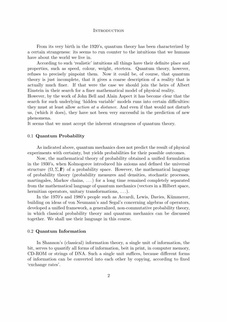
Introduction

From its very birth in the 1920’s, quantum theory has been characterized bya certain strangeness: its seems to run counter to the intuitions that we humanshave about the world we live in.

According to such ‘realistic’ intuitions all things have their definite place andproperties, such as speed, colour, weight, etcetera. Quantum theory, however,refuses to precisely pinpoint them. Now it could be, of course, that quantumtheory is just incomplete, that it gives a coarse description of a reality that isactually much finer. If that were the case we should join the heirs of AlbertEinstein in their search for a finer mathematical model of physical reality.However, by the work of John Bell and Alain Aspect it has become clear that thesearch for such underlying ‘hidden variable’ models runs into certain difficulties:they must at least allow action at a distance. And even if that would not disturbus, (which it does), they have not been very successful in the prediction of newphenomena.It seems that we must accept the inherent strangeness of quantum theory.

0.1 Quantum Probability

As indicated above, quantum mechanics does not predict the result of physicalexperiments with certainty, but yields probabilities for their possible outcomes.

Now, the mathematical theory of probability obtained a unified formulationin the 1930’s, when Kolmogorov introduced his axioms and defined the universalstructure (Ω,Σ, IP) of a probability space. However, the mathematical languageof probability theory (probability measures and densities, stochastic processes,martingales, Markov chains, . . .) for a long time remained completely separatedfrom the mathematical language of quantum mechanics (vectors in a Hilbert space,hermitian operators, unitary transformations, . . .).

In the 1970’s and 1980’s people such as Accardi, Lewis, Davies, Kummerer,building on ideas of von Neumann’s and Segal’s concerning algebras of operators,developed a unified framework, a generalized, non-commutative probability theory,in which classical probability theory and quantum mechanics can be discussedtogether. We shall use their language in this course.

0.2 Quantum Information

In Shannon’s (classical) information theory, a single unit of information, thebit, serves to quantify all forms of information, beit in print, in computer memory,CD-ROM or strings of DNA. Such a single unit suffices, because different formsof information can be converted into each other by copying, according to fixed‘exchange rates’.

2

The physical states of quantum systems, however, cannot be copied into such‘classical’ information, but can be converted into one another. This leads to a newunit of information: the qubit.

Quantum Information theory studies the handling of this new form of infor-mation by information-carrying ‘channels’.

0.3 Quantum Computing

It was Richard Feynman who first thought of actually employing the strange-ness of quantum mechanics to do things that would be impossible in a classicalworld.

The idea was developed in the 1980’s and 1990’s by David Deutsch, Peter Shor,and many others into a flourishing branch of science called ‘quantum computing’:how to make quantummechanical systems perform calculations more efficientlythan ordinary computers can. This research is still in a predominantly theoreticalstage: the quantum computers actually built are as yet extremely primitive and canby no means compete with even the simplest pocket calculator, but expectationsare high.

0.4 This course

We start with an introduction to quantum probability. No prior knowledgeof quantummechanics is assumed; what is needed will be explained in the course.

We begin by demonstrating the ‘strangeness’ of quantum phenomena by verysimple polarization experiments, culminating in Bell’s famous inequality, tested inAspect’s equally famous experiment. Bell’s inequality is a statement in classicalprobability that is violated in quantum probability and in reality.

Taking polarizers as our starting point, we build up our new probability theoryin terms of algebras of operators on a Hilbert space.

Operations on these algebras will then be characterized, and the points wherethey are at variance with classical operations: what cannot be done with them(copying, coding into classical information, joint measurement of incompatibleobservables, measurement without perturbing the measured object), and what canbe done (entangling remote systems, teleportation of this entanglement, sendingtwo bits in a single qubit). Then luring perspectives will be sketched: highlyefficient algorithms for sorting, Fourier transformation and factoring very largenumbers.

As an example of quantum thinking we shall treat a quantum version of thefamous ‘three door’ or ‘Monty Hall’ riddle.

We shall introduce the concepts of entropy and information in the classicaland the quantum context. We shall describe simple quantum Markov chains andtheir relation to repeated measurement and quantum counting processes. These

3

will lead to the so-called quantum trajectories: simulation of quantum processeson a (classical) computer.

If time permits we shall go into some of the following topics:(i) entropic uncertainty relations,(ii) quantum error correction,(iii) stochastic Schrodinger equations, and(iv) ergodicity of quantum trajectories.

4

1. Why Classical Probability does not Suffice *

1.1 An experiment with polarisers

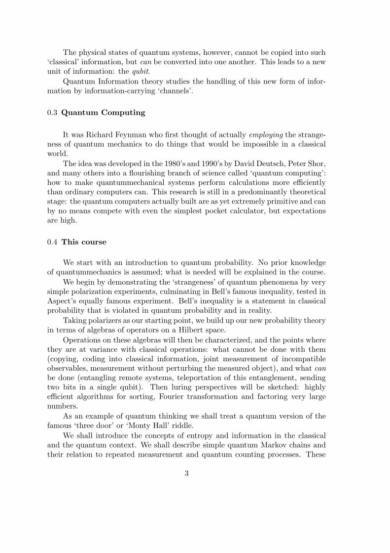
To start with, we consider a simple experiment. In a beam of light of a fixedcolour we put a pair of polarizing filters, each of which can be rotated around theaxis formed by the beam. As is well known, the light which comes through bothfilters differs in intensity when the filters are rotated relative to each other. Ifwe fix the first filter and rotate the second, then we see that there is a directionwhere the resulting intensity is maximal. Starting from this position, and rotatingthe second filter through an angle α , the light intensity decreases with α until itvanishes for α = 1

2π . Careful measurement shows that the intensity of the lightpassing the first filter is half the beam intensity (we assume the original beamto be completely unpolarized) and that of the light passing the second filter isproportional to cos2 α . If we call the intensity of the beam before the filters I0 ,after the first I1 , and after the second I2 , then I1 = 1

2I0 and

I2 = I1 cos2 α. (1)

II I0 1 2α

fig. 1

Now, it has been observed that for extremely low intensities (monochromatic)light comes in small packages, called photons, all of the same energy, (which isindependent of the total intensity).So the intensity must be proportional to the number of photons, and formula (1)has to be given a statistical meaning: a photon passing through the first filter has

* This chapter is based on: B. Kummerer and H. Maassen, Elements of Quan-tum Probability, Quantum Probability Communications, X pp. 73–100.

5

a probability cos2 α to pass through the second. So formula (1) only holds on theaverage, i.e., for large numbers of photons.

If we think along the lines of classical probability, then we may attach to apolarization filter in the direction α a random variable Pα , taking the values 0and 1, where Pα(ω) = 0 if the photon ω is absorbed by the filter and Pα(ω) = 1if it passes through. For two filters in the directions α and β we may write fortheir correlation:

IE(PαPβ) = IP[Pα = 1 and Pβ = 1] = 12

cos2(α− β).

(Here a common notation from probability theory is used, namely, the expression[Pα = 1 and Pβ = 1] stands for the set of those ω for which Pα(ω) = 1 andPβ(ω) = 1.)

The following argument shows that this line of reasoning leads into difficulties.Take three polarizing filters F1 , F2 , and F3 , having polarization directions α1 ,α2 and α3 respectively. We put them on the optical bench in pairs. Then theygive rise to random variables P1 , P2 and P3 satisfying

IE(PiPj) = 12

cos2(αi − αj).

Proposition (Bell’s 3 variable inequality) For any three 0-1-valued randomvariables P1 , P2 , and P3 on a probability space (Ω, IP) the following inequalityholds:

IP[P1 = 1, P3 = 0] ≤ IP[P1 = 1, P2 = 0] + IP[P2 = 1, P3 = 0].

Proof. Write

IP[P1 = 1, P3 = 0] = IP[P1 = 1, P2 = 0, P3 = 0] + IP[P1 = 1, P2 = 1, P3 = 0]

≤ IP[P1 = 1, P2 = 0] + IP[P2 = 1, P3 = 0].

In our example, however, we have

IP[Pi = 1, Pj = 0] = IP[Pi = 1]− IP[Pi = 1, Pj = 1]

= 12 − 1

2 cos2(αi − αj) = 12 sin2(αi − αj).

Bell’s inequality thus reads

12

sin2(α1 − α3) ≤ 12

sin2(α1 − α2) + 12

sin2(α2 − α3),

which is clearly violated for α1 = 0, α2 = 16π and α3 = 1

3π , where it becomes

3

8≤ 1

8+

1

8.

6

We thus come to the conclusion that classical probability cannot describe thissimple experiment!

RemarkThe above calculation could be summarized as follows: we are in fact looking

for a family of 0-1-valued random variables (Pα)0≤α<π with IP[Pα = 1] = 12,

satisfying the requirement that

IP[Pα 6= Pβ ] = sin2(α− β).

Now, on the space of 0-1-valued random variables on a probability space the func-tion (X,Y ) 7→ IP[X 6= Y ] equals the L1 -distance of X and Y :

IP[X 6= Y ] =

∫

Ω

|X(ω)− Y (ω)| IP(dω) = ‖X − Y ‖1.

On the other hand, the function (α, β) 7→ sin2(α−β) does not satisfy the triangleinequality for a metric on the interval [0, π). Therefore no family (Pα)0≤α<πexists which meets the above requirement.

1.2 An improved experiment

A possible criticism to the above argument runs as follows. Are the randomvariables Pα well-defined? Is it indeed true that for each photon ω and eachfilter Fα it is determined whether ω passes through Fαor not? Could not filterFα influence the photon’s reaction to filter Fβ ? In fact, it seems quite obviousthat it will!

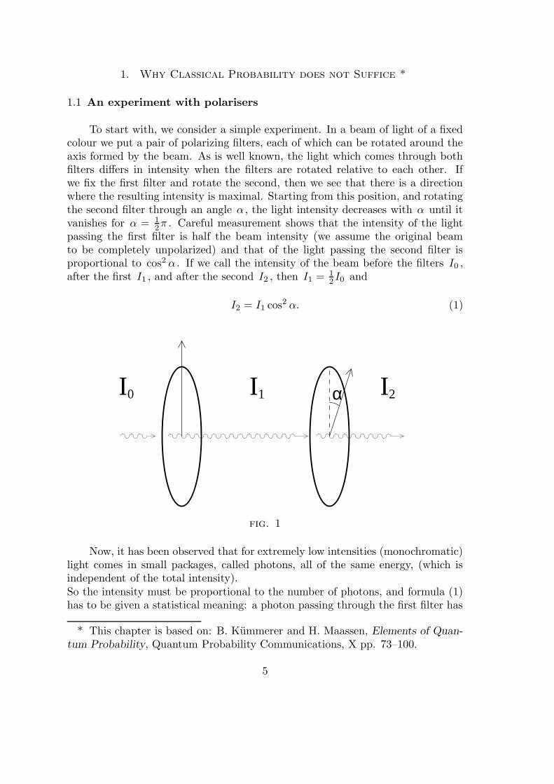
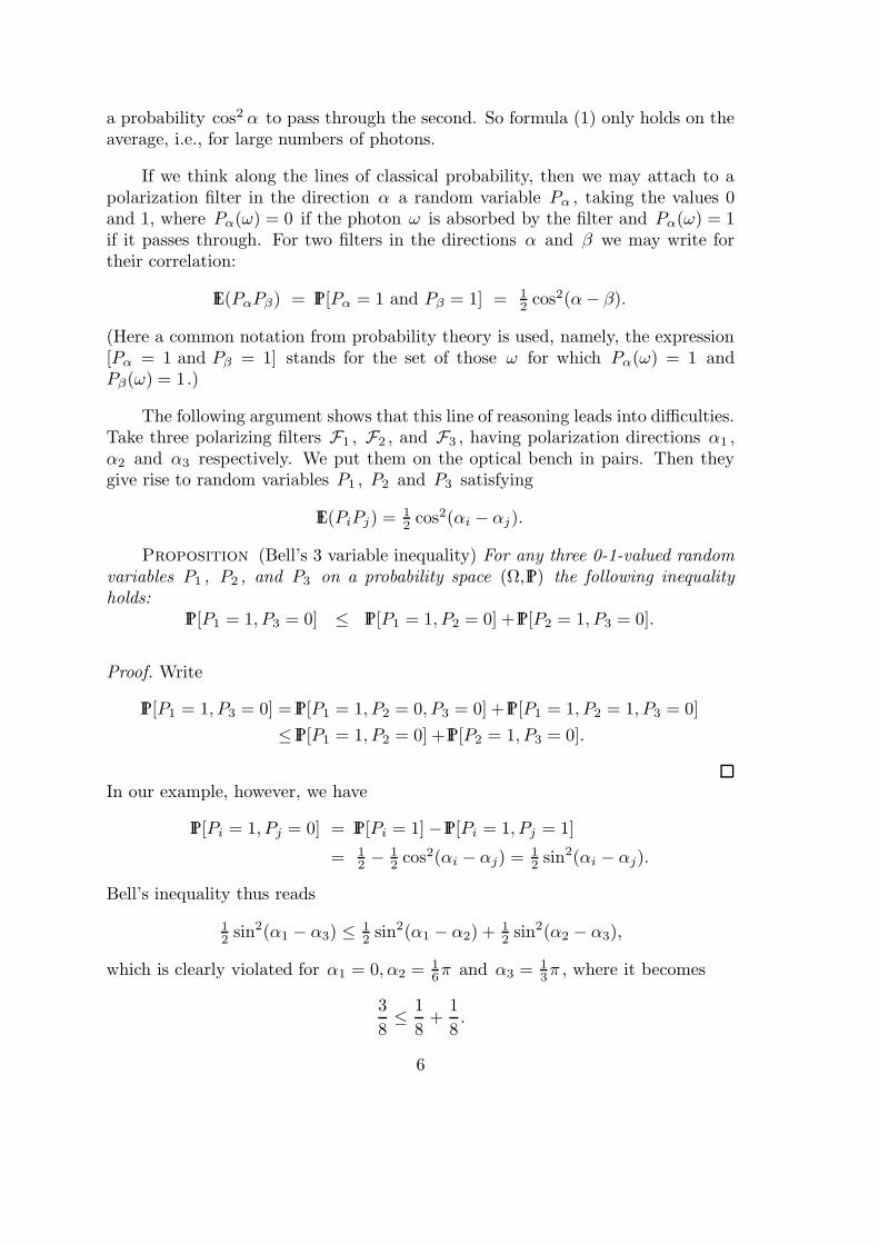
In order to meet this criticism we should do a better experiment. We shouldlet the filters act on each of the photons without influence on each other.A clever technique from quantum optics comes to our aid. It is possible to builda device that produces pairs of photons, such that the members of each pair movein opposite directions and show opposite behaviour towards polarization filters:if one passes the filter, then the other is surely absorbed. The device containsCalcium atoms, which are excited by a laser to a state they can only leave underemission of such a pair.

α β

Ca

7

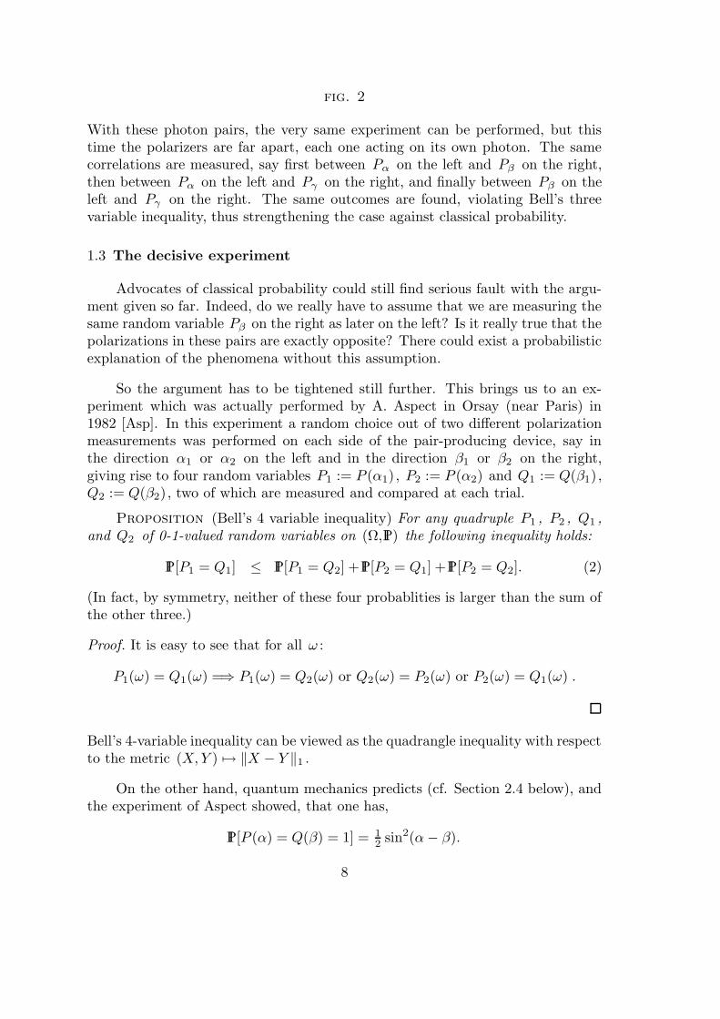
fig. 2

With these photon pairs, the very same experiment can be performed, but thistime the polarizers are far apart, each one acting on its own photon. The samecorrelations are measured, say first between Pα on the left and Pβ on the right,then between Pα on the left and Pγ on the right, and finally between Pβ on theleft and Pγ on the right. The same outcomes are found, violating Bell’s threevariable inequality, thus strengthening the case against classical probability.

1.3 The decisive experiment

Advocates of classical probability could still find serious fault with the argu-ment given so far. Indeed, do we really have to assume that we are measuring thesame random variable Pβ on the right as later on the left? Is it really true that thepolarizations in these pairs are exactly opposite? There could exist a probabilisticexplanation of the phenomena without this assumption.

So the argument has to be tightened still further. This brings us to an ex-periment which was actually performed by A. Aspect in Orsay (near Paris) in1982 [Asp]. In this experiment a random choice out of two different polarizationmeasurements was performed on each side of the pair-producing device, say inthe direction α1 or α2 on the left and in the direction β1 or β2 on the right,giving rise to four random variables P1 := P (α1), P2 := P (α2) and Q1 := Q(β1),Q2 := Q(β2), two of which are measured and compared at each trial.

Proposition (Bell’s 4 variable inequality) For any quadruple P1 , P2 , Q1 ,and Q2 of 0-1-valued random variables on (Ω, IP) the following inequality holds:

IP[P1 = Q1] ≤ IP[P1 = Q2] + IP[P2 = Q1] + IP[P2 = Q2]. (2)

(In fact, by symmetry, neither of these four probablities is larger than the sum ofthe other three.)

Proof. It is easy to see that for all ω :

P1(ω) = Q1(ω) =⇒ P1(ω) = Q2(ω) or Q2(ω) = P2(ω) or P2(ω) = Q1(ω) .

Bell’s 4-variable inequality can be viewed as the quadrangle inequality with respectto the metric (X,Y ) 7→ ‖X − Y ‖1 .

On the other hand, quantum mechanics predicts (cf. Section 2.4 below), andthe experiment of Aspect showed, that one has,

IP[P (α) = Q(β) = 1] = 12 sin2(α− β).

8

Similarly, IP[P (α) = Q(β) = 0] = 12 sin2(α− β). Hence

IP[P (α) = Q(β)] = sin2(α− β).

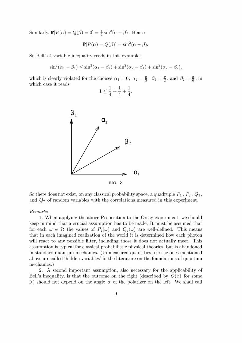
So Bell’s 4 variable inequality reads in this example:

sin2(α1 − β1) ≤ sin2(α1 − β2) + sin2(α2 − β1) + sin2(α2 − β2),

which is clearly violated for the choices α1 = 0, α2 = π3 , β1 = π

2 , and β2 = π6 , in

which case it reads

1 ≤ 1

4+

1

4+

1

4.

1

2

2

1α

β

αβ

fig. 3

So there does not exist, on any classical probability space, a quadruple P1 , P2 , Q1 ,and Q2 of random variables with the correlations measured in this experiment.

Remarks.1. When applying the above Proposition to the Orsay experiment, we should

keep in mind that a crucial assumption has to be made. It must be assumed thatfor each ω ∈ Ω the values of Pj(ω) and Qj(ω) are well-defined. This meansthat in each imagined realization of the world it is determined how each photonwill react to any possible filter, including those it does not actually meet. Thisassumption is typical for classical probabilistic physical theories, but is abandonedin standard quantum mechanics. (Unmeasured quantities like the ones mentionedabove are called ‘hidden variables’ in the literature on the foundations of quantummechanics.)

2. A second important assumption, also necessary for the applicability ofBell’s inequality, is that the outcome on the right (described by Q(β) for someβ ) should not depend on the angle α of the polarizer on the left. We shall call

9

this assumption ‘locality’. In order to justify this assumption, Aspect has madeconsiderable efforts. In his (third) experiment, the choice of what to measureon the left (α1 or α2 ) and on the right (β1 or β2 ) was made during the flightof the photons, so that any influence which each of these choices might have onthe outcome on the opposite end would have to travel faster than light. By thecausality principle of Relativity Theory such influences are not possible.

3. Clearly, the above reasoning does not exclude the possibility of an expla-nation of the experiment in classical probabilistic terms, if one is willing to giveup the causality principle. Serious attempts have been made in this direction (e.g.[Boh]).

10

1.4 The Orsay experiment as a card game

It has now become very difficult for the advocates of classical probabilityto criticize the experiment. To illustrate this point, we shall again present theexperiment, but this time in the form of a card game. Nature can win this game.Can you?

11010011000110100100011

00110010011100101100101

0110101110010.......

00110011011010010110101

011101100111101001100001

110110001011101000111101

011010011001010111010010

110101010110011......

110001011.....

11010011010001101011110

01110010100101110101101

110100011011001101001101

000101110000100....

Q

red

11 12

22

110000100101110000101001

100001000100101100101001

black

red

black

P

a a

21a a

fig. 4

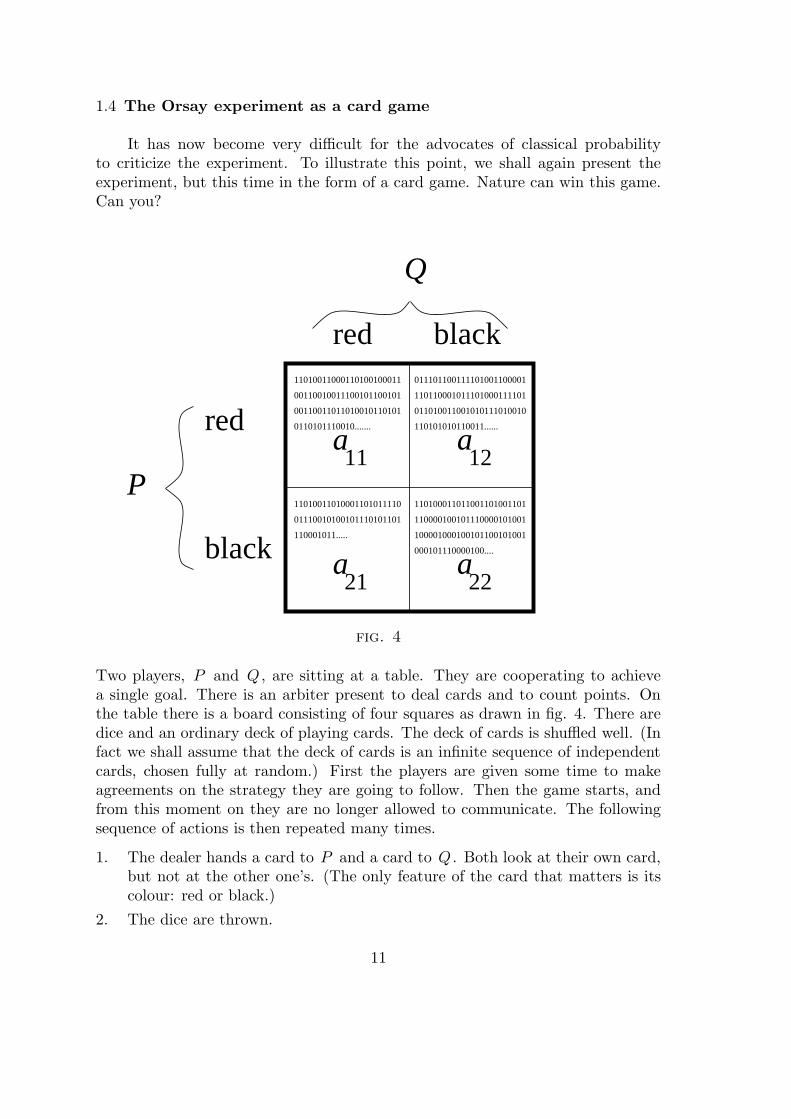
Two players, P and Q , are sitting at a table. They are cooperating to achievea single goal. There is an arbiter present to deal cards and to count points. Onthe table there is a board consisting of four squares as drawn in fig. 4. There aredice and an ordinary deck of playing cards. The deck of cards is shuffled well. (Infact we shall assume that the deck of cards is an infinite sequence of independentcards, chosen fully at random.) First the players are given some time to makeagreements on the strategy they are going to follow. Then the game starts, andfrom this moment on they are no longer allowed to communicate. The followingsequence of actions is then repeated many times.

1. The dealer hands a card to P and a card to Q . Both look at their own card,but not at the other one’s. (The only feature of the card that matters is itscolour: red or black.)

2. The dice are thrown.

11

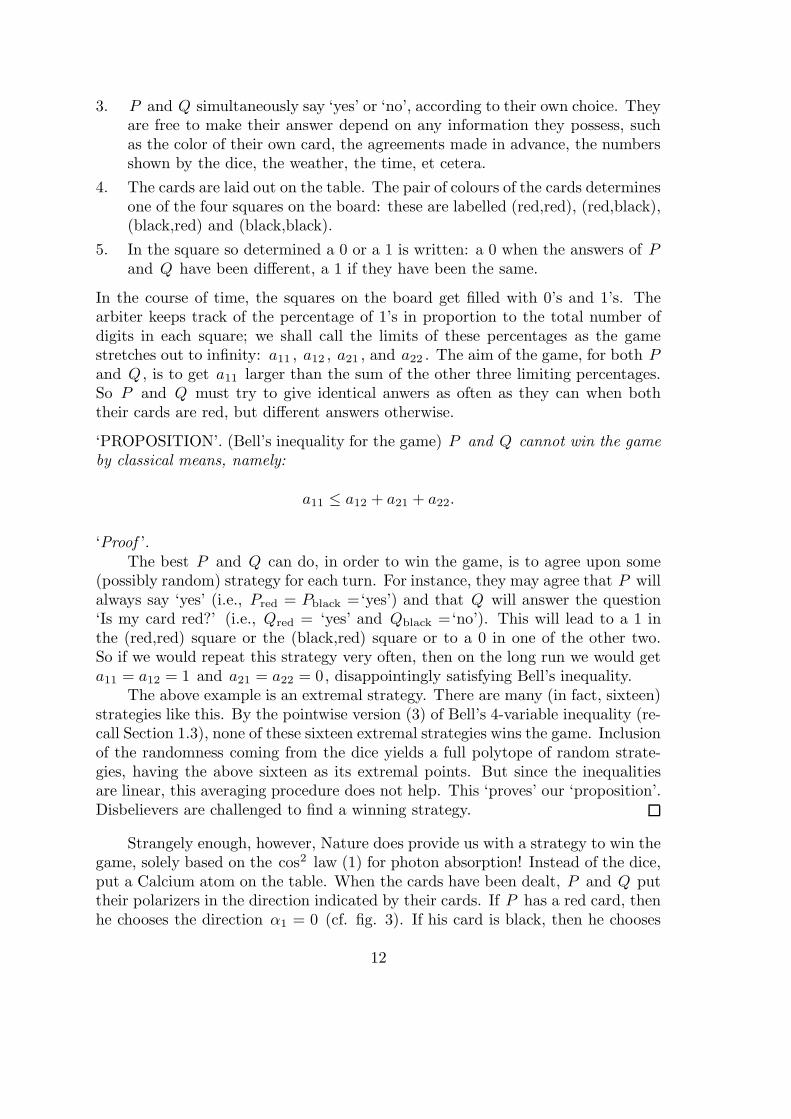
3. P and Q simultaneously say ‘yes’ or ‘no’, according to their own choice. Theyare free to make their answer depend on any information they possess, suchas the color of their own card, the agreements made in advance, the numbersshown by the dice, the weather, the time, et cetera.

4. The cards are laid out on the table. The pair of colours of the cards determinesone of the four squares on the board: these are labelled (red,red), (red,black),(black,red) and (black,black).

5. In the square so determined a 0 or a 1 is written: a 0 when the answers of Pand Q have been different, a 1 if they have been the same.

In the course of time, the squares on the board get filled with 0’s and 1’s. Thearbiter keeps track of the percentage of 1’s in proportion to the total number ofdigits in each square; we shall call the limits of these percentages as the gamestretches out to infinity: a11 , a12 , a21 , and a22 . The aim of the game, for both Pand Q , is to get a11 larger than the sum of the other three limiting percentages.So P and Q must try to give identical anwers as often as they can when boththeir cards are red, but different answers otherwise.

‘PROPOSITION’. (Bell’s inequality for the game) P and Q cannot win the gameby classical means, namely:

a11 ≤ a12 + a21 + a22.

‘Proof ’.The best P and Q can do, in order to win the game, is to agree upon some

(possibly random) strategy for each turn. For instance, they may agree that P willalways say ‘yes’ (i.e., Pred = Pblack =‘yes’) and that Q will answer the question‘Is my card red?’ (i.e., Qred = ‘yes’ and Qblack =‘no’). This will lead to a 1 inthe (red,red) square or the (black,red) square or to a 0 in one of the other two.So if we would repeat this strategy very often, then on the long run we would geta11 = a12 = 1 and a21 = a22 = 0, disappointingly satisfying Bell’s inequality.

The above example is an extremal strategy. There are many (in fact, sixteen)strategies like this. By the pointwise version (3) of Bell’s 4-variable inequality (re-call Section 1.3), none of these sixteen extremal strategies wins the game. Inclusionof the randomness coming from the dice yields a full polytope of random strate-gies, having the above sixteen as its extremal points. But since the inequalitiesare linear, this averaging procedure does not help. This ‘proves’ our ‘proposition’.Disbelievers are challenged to find a winning strategy.

Strangely enough, however, Nature does provide us with a strategy to win thegame, solely based on the cos2 law (1) for photon absorption! Instead of the dice,put a Calcium atom on the table. When the cards have been dealt, P and Q puttheir polarizers in the direction indicated by their cards. If P has a red card, thenhe chooses the direction α1 = 0 (cf. fig. 3). If his card is black, then he chooses

12

α2 = π3 . If Q has a red card, then he chooses β1 = π

2 . If his card is black, then hechooses β2 = π

6. No information on the colours of the cards needs to be exchanged.

When the Calcium atom has produced its photon pair, each player looks whetherhis own photon passes his own polarizer, and then says ‘yes’ if it does, ‘no’ if itdoes not. On the long run they will get a11 = 1, a12 = a21 = a22 = 1

4 , and thusthey win the game.

So the Calcium atom, the quantummechanical die, makes possible what couldnot be done with the classical die.

13

2. Towards a Mathematical Model

2.1 A mathematical description of polarization

Coerced by the foregoing considerations, we give up trying to make a classicalprobabilistic model in order to explain polarization experiments. Instead, we takethese experiments as a paradigm for an alternative type of probability, to bedeveloped now.

We have discussed (linear) polarization of a light beam. This is completelycharacterized by a direction in the plane perpendicular to the light beam. Thissuggests that we should describe different directions of polarization by differentdirections in a two-dimensional real plane IR2 , or equivalently by unit vectorsψ ∈ IR2 , ‖ψ‖ = 1, pointing in this direction. Moreover, it appears that we cannotphysically distinguish between two states which differ by a rotation of π , so wehave to describe states of polarizations by one-dimensional subspaces of IR2 . (Twounit vectors span the same one-dimensional subspace if they differ only by a sign.)Given two directions of polarization with an angle α between them, spanned bytwo unit vectors ψ, θ ∈ IR2 , the transition probability cos2 α can be expressed as

cos2 α = <ψ, θ>2

where < ψ, θ > denotes the scalar product between ψ and θ . (Since cos2 α =cos2(π − α), this expression does not depend on the sign of ψ, θ .)

Certainly, in order to come to a mathematical model we should distinguishbetween the physical state of polarization of a photon on the one hand and thefilter on the other hand, i.e., the 0-1-valued random variable which asks, whethera photon is polarized in a certain direction. This can be done by identifyingthe filter, (i.e., the random variable), with the orthogonal projection P onto theone-dimensional subspace. We can then write

cos2 α = <ψ, θ>2 = < ψ,Pψ> .

So we arrive at the following mathematical model:

States of polarization of a photon = one-dimensional subspaces of IR2 descri-bed by unit vectors ψ spanning the sub-space.

Polarization filters, (i.e., random va-riables measuring polarization)

= orthogonal projections P from IR2 ontothe corresponding one-dimensional sub-space.

Probability that a photon, describedby ψ , passes through the filter de-scribed by P

= < ψ,Pψ> = cos2 α .

14

Since P is 0-1-valued, (i.e., a photon passes or is absorbed), this probabilityis equal to the expectation of this random variable:

< ψ,Pψ> = IE(P ) .

It is important to realize that, although we gave a kind of proof (in Section 1)that polarization experiments cannot be described by classical random variableson classical probability spaces, there is no logical argument that photons mustbe described by vectors and filters by projections, as we just did. Indeed, sincethe beginnings of quantum mechanics there have been many efforts to developalternative mathematical models. We are going to describe here the traditionalpoint of view of quantum mechanics [Neu]. This will lead to a mathematical modelwhich extends classical probability and up until now has described experimentscorrectly.

2.2 The full quantum mechanical truth about polarization: the qubit

In the foregoing description of polarization things were presented somewhatsimpler than they are: we considered only linear polarization, thus disregardingcircular polarization. The full description of polarization leads to the quantummechanics of a 2-level system or qubit:

State of polarization of a photon = one-dimensional subspace of C2 , descri-bed by a unit vector ψ spanning thissubspace (and determined only up to aphase).

Polarization filter or generalized 0-1-valued random variable

= orthogonal projection P onto a complexone-dimensional subspace.

(Also for left- or right-circular polarization do there exist physical filters.)

Probability for a photon, describedby ψ , to pass through a filter, de-scribed by P

= < ψ,Pψ> .

The set of all states is conveniently parametrized by the unit vectors of theform

(cosα, eiφ sinα) ∈ C2 ,−π2≤ α ≤ π

2, 0 ≤ φ ≤ π .

This set can be identified with the points on the unit sphere S2 ∈ IR3 when usingthe polar coordinates θ = 2α and φ . Restricting to states with φ = 0, (whichare parametrized by the points of the circle (cos 2α, sin 2α) in IR2 ), we retain theforegoing real description when we identify α with the angle of polarization.

A possible identification of the points of S2 ⊆ IR3 with physical states, givingthe correct values for all probabilities, is as in the picture below:

15

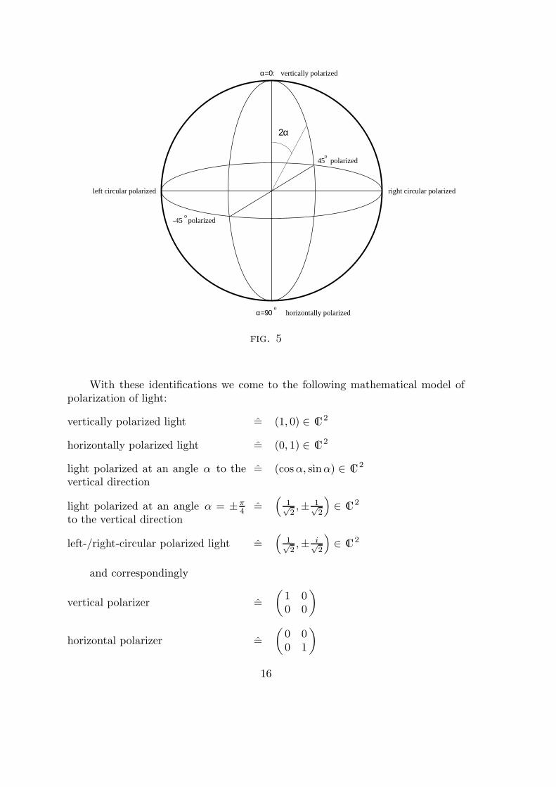
2α

α=0: vertically polarized

left circular polarized right circular polarized

45 polarized

-45 polarized

o

horizontally polarizedα=90o

o

fig. 5

With these identifications we come to the following mathematical model ofpolarization of light:

vertically polarized light = (1, 0) ∈ C2

horizontally polarized light = (0, 1) ∈ C2

light polarized at an angle α to thevertical direction

= (cosα, sinα) ∈ C2

light polarized at an angle α = ±π4to the vertical direction

=(

1√2,± 1√

2

)∈ C2

left-/right-circular polarized light =(

1√2,± i√

2

)∈ C2

and correspondingly

vertical polarizer =

(1 00 0

)

horizontal polarizer =

(0 00 1

)

16

angle-α -polarizer =

(cos2 α cosα sinα

cosα sinα sin2 α

)

±π4-polarizer =

(12± 1

2± 1

212

)

left/right circular polarizer =

(12 ∓ i

2

± i2

12

)

2.3 Finite dimensional models

The mathematical model that is used by quantum mechanics is the straight-forward generalization of the above description. In order to keep things simple,we restrict ourselves to the quantum mechanics of finite dimensions. It generalizesthe probability theory of systems with only finitely many states. As in classicalprobability, the generalization to systems with a countable number of states or acontinuum of states is analytically more involved, though conceptually easy.

The model is as follows:

States correspond to one-dimensional subspaces of Cn , where the dimensionn is determined by the model. Again, a state is described conveniently by someunit vector spanning this subspace.

0-1-valued random variables are described by orthogonal projections ontoa linear subspace of Cn . If the random variable only asks whether the system isin a certain state, then the subspace is one-dimensional. But also projections ontohigher dimensional subspaces K make sense. They answer the question whetherthe system is in any of the states represented by a unit vector in K . Similarquestions for other subsets of states are not allowed!

The probability that a measurement of a random variable P on a system ina state ψ gives the value 1 is still given by < ψ,Pψ> .

Note that we do not assume that every unit vector ψ ∈ Cn describes a stateof the system, nor that every orthogonal projection corresponds to a meaningfulrandom variable. Specializing these two sets is part of the description of themathematical model for a given system. In a truly quantum mechanical situation,typically all possible vectors and projections are used. In contrast to this, a modelfrom classical probability is incorporated into this description as follows.

2.4 Finite classical models

A finite probability space is usually described by a finite set Ω = ω1, . . . , ωnand a probability distribution (p1, . . . , pn), 0 ≤ pi ≤ 1,

∑i pi = 1, such that the

probability for ωi is pi . A 0-1-valued random variable is a 0-1-valued function on

17

Ω, i.e., a characteristic function χA of some subset A ⊆ Ω. In order to describesuch a system in our model, we think of Cn as the space of complex valuedfunctions on Ω, and use the functions δi with δi(ωj) = δi,j as basis. The statesof the system, i.e., the points ωi of Ω, are now represented by the unit vectors δi ,1 ≤ j ≤ n . The random variable χA is identified with the orthogonal projectionPA onto the linear span of the vectors δi : ωi ∈ A . In our basis χA becomesa diagonal matrix with a 1 at the i -th place of the diagonal if ωi ∈ A , and a0 otherwise. It is obvious that ωi ∈ A if and only if χA(ωi) = 1 if and only if< δi, PAδi> = 1.

Conversely, any set of pairwise commuting projections on Cn can be diagonal-ized simultaneously and thus have an interpretation as a set of classical 0-1-valuedrandom variables. Therefore:

Classical probability corresponds to sets of pairwise commuting projections.

In the above sketch of classical probability an important point is obviouslymissing: So far we have only considered pure states of the system, a probabilitydistribution (p1, . . . , pn) did not enter the dicussion. How can we describe asituation where a system is in a certain state ψ with probability q and in anotherstate y with probability 1− q (0 ≤ q ≤ 1) ?

Obviously, the set of states should be a convex set, containing also the mixedstates. In the classical model of probability, the appropriate convex combinationsof point measures are taken in order to obtain a new probability measure.

In general, if P is any 0-1-valued (quantum) random variable and ψ1, . . . , ψkare arbitrary quantum states, each occuring with a probability pi , 1 ≤ i ≤ k ,∑i pi = 1, pi ≥ 0, then the probability that a measurement of P gives 1 is

clearly given by ∑

i

pi < ψi, Pψi> .

A more convenient description of mixed states is obtained as follows.For a unit vector ψ ∈ Cn denote by Φψ the orthogonal projection onto

the one-dimensional subspace generated by ψ . In the physics literature, Φψ isfrequently denoted by |ψ><ψ| . By tr denote the trace on the n × n -matrices,summing up the diagonal entries of such a matrix. Then one obtains

< ψ,Pψ> = tr(Φψ · P ) .

Hence ∑

i

pi < ψi, Pψi> = tr(∑

i

piΦψi· P ) = tr(Φ · P ) ,

where Φ :=∑i piΦψi

.Being a convex combination of 1-dimensional projections, Φ obviously is a

positive (i.e., self-adjoint positive semidefinite) n × n -matrix with tr(Φ) = 1.Conversely, from diagonalizing positive matrices it is clear that any such positive

18

matrix Φ with tr(Φ) = 1 can be written as a convex combination of 1-dimensionalprojections. The set of these matrices forms a closed (even compact) convex set,and its extreme points are precisely the 1-dimensional projections which in turncorrespond to pure states, represented also by unit vectors. Therefore it is preciselythis class of matrices which represents mixed states. These matrices are frequentlycalled density matrices.

Thus, a general mixed state is described by a density matrix Φ and theprobability for an observation of P to yield the value 1 is given by tr(Φ · P ).

Remarks

1. Although in this description also pure states are described by 1-dimensionalprojections, they are not considered as random variables.

2. The decomposition of a density matrix Φ into a convex combination of 1-dimensional projections is by no means unique. The compact convex set of densitymatrices is far from being a simplex. Indeed, on C2 it can be affinely identifiedwith a full ball in IR3 , by taking in IR3 the convex hull of the sphere that wasdescribed above.

3. In classical probability the convex set of mixed states is the simplex ofall probability distributions. In our picture, if we insist on decomposing a mixedstate given by Φ =

∑i piPδi

into a convex combination of pure states (within theconvex hull of Pδi

: 1 ≤ i ≤ n which is a simplex), then it becomes unique.

4. Physically, a state Φ is completely described by all of its values tr(Φ ·P ),where P runs through the random variables of the model. Thus, if we consideronly subsets of projections, then two different density matrices can represent thesame physical state of the system. As a drastic example, consider the classicalsystem Ω = ω1, . . . , ωn with equidistribution, i.e., pi(ωi) = 1

n , leading to thedensity matrix Φ =

∑i

1nPδi

= 1n· 1l. On the other hand, with the unit vector

ψ = ( 1√n, . . . , 1√

n) ∈ Cn , we obtain for any subset A ⊆ Ω: tr(Φ ·PA) = 1

n · |A| =< ψ,PAψ> . Therefore, on the random variables PA : A ⊆ Ω , the rank-one-density matrix Pψ represents the same state as the densitiy matrix 1

n· 1l. Note,

however, that Pψ is not in the convex hull of Pδi: 1 ≤ i ≤ n .

2.5 The mathematical model of Aspect’s experiment

As an illustration, we shall now explain the photon correlation in the Orsayexperiment, given by the cos2 -law. Note that here we cannot simply refer to thebasic cos2 -law of quantum probability, since the filters are acting on two differentphotons.

The polarization of a pair of photons is described by a unit vector in the

19

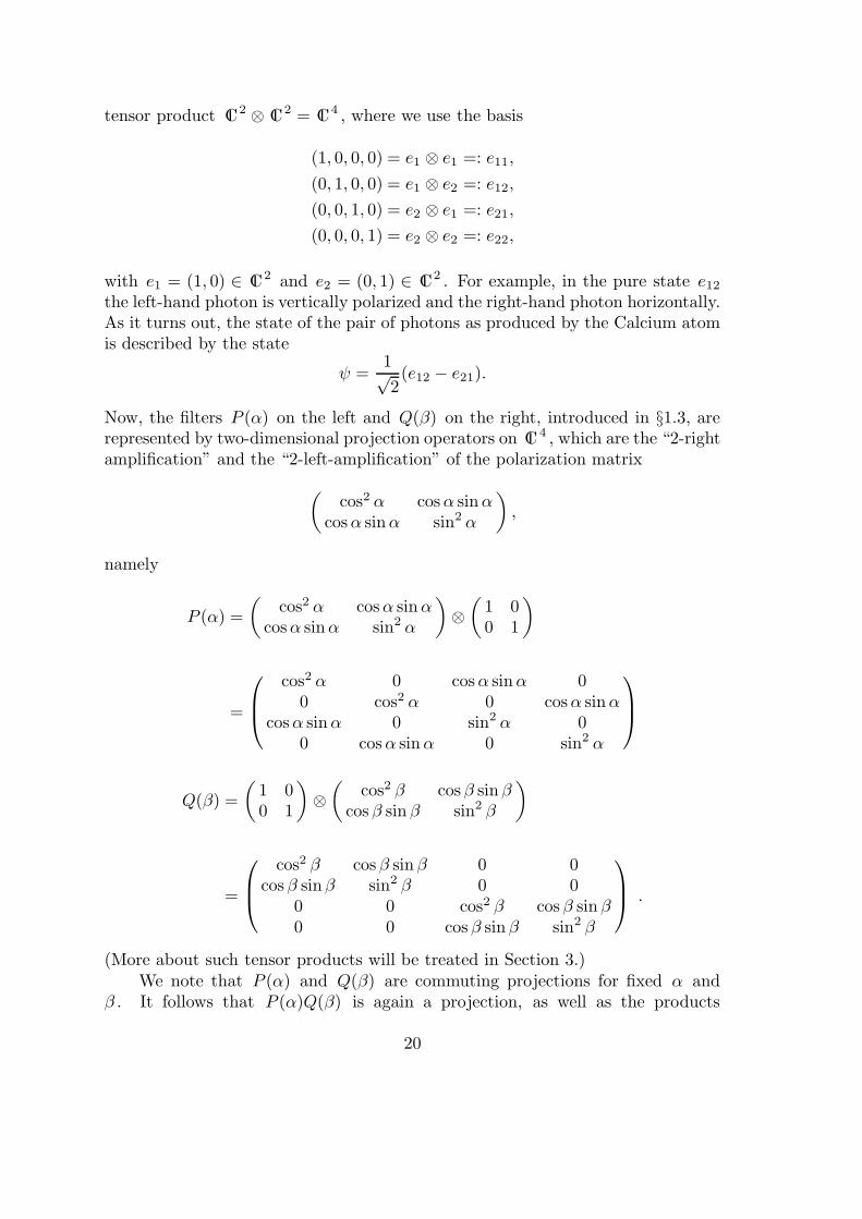
tensor product C2 ⊗ C2 = C4 , where we use the basis

(1, 0, 0, 0) = e1 ⊗ e1 =: e11,

(0, 1, 0, 0) = e1 ⊗ e2 =: e12,

(0, 0, 1, 0) = e2 ⊗ e1 =: e21,

(0, 0, 0, 1) = e2 ⊗ e2 =: e22,

with e1 = (1, 0) ∈ C2 and e2 = (0, 1) ∈ C2 . For example, in the pure state e12the left-hand photon is vertically polarized and the right-hand photon horizontally.As it turns out, the state of the pair of photons as produced by the Calcium atomis described by the state

ψ =1√2(e12 − e21).

Now, the filters P (α) on the left and Q(β) on the right, introduced in §1.3, arerepresented by two-dimensional projection operators on C 4 , which are the “2-rightamplification” and the “2-left-amplification” of the polarization matrix

(cos2 α cosα sinα

cosα sinα sin2 α

),

namely

P (α) =

(cos2 α cosα sinα

cosα sinα sin2 α

)⊗(

1 00 1

)

=

cos2 α 0 cosα sinα 00 cos2 α 0 cosα sinα

cosα sinα 0 sin2 α 00 cosα sinα 0 sin2 α

Q(β) =

(1 00 1

)⊗(

cos2 β cos β sin βcos β sin β sin2 β

)

=

cos2 β cos β sin β 0 0cos β sinβ sin2 β 0 0

0 0 cos2 β cos β sin β0 0 cos β sin β sin2 β

.

(More about such tensor products will be treated in Section 3.)We note that P (α) and Q(β) are commuting projections for fixed α and

β . It follows that P (α)Q(β) is again a projection, as well as the products

20

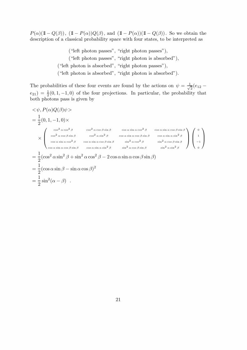
P (α)(1l−Q(β)), (1l− P (α))Q(β), and (1l − P (α))(1l− Q(β)). So we obtain thedescription of a classical probability space with four states, to be interpreted as

(“left photon passes”, “right photon passes”),

(“left photon passes”, “right photon is absorbed”),

(“left photon is absorbed”, “right photon passes”),

(“left photon is absorbed”, “right photon is absorbed”).

The probabilities of these four events are found by the actions on ψ = 1√2(e12 −

e21) = 12 (0, 1,−1, 0) of the four projections. In particular, the probability that

both photons pass is given by

<ψ,P (α)Q(β)ψ>

=1

2(0, 1,−1, 0)×

×

cos2 α cos

2 β cos2 α cos β sin β cos α sin α cos

2 β cos α sin α cos β sin β

cos2 α cos β sin β cos

2 α sin2 β cos α sin α cos β sin β cos α sin α sin

2 β

cos α sin α cos2 β cos α sin α cos β sin β sin

2 α cos2 β sin

2 α cos β sin β

cos α sin α cos β sin β cos α sin α sin2 β sin

2 α cos β sin β sin2 α sin

2 β

0

1

−1

0

=1

2(cos2 α sin2 β + sin2 α cos2 β − 2 cosα sinα cos β sin β)

=1

2(cosα sin β − sinα cos β)2

=1

2sin2(α− β) .

21

3. Quantum Probability

In classical probability a model — or probability space — is determined by givinga set Ω of outcomes ω , by specifying what subsets S ⊂ Ω are to be considered asevents, and by associating a probability IP(S) to each of these events. Requirements:the events must form a σ -algebra and the probability measure IP must be σ -additive.In quantum probability we must loosen this scheme somewhat.We must give up the set Ω of sample points: a point ω ∈ Ω in a classical model de-cides about the occurrence or non-occurrence of all events simultaneously, and thiswe abandon. Following our polarization example of Chapter 2 we take as eventscertain closed subspaces of a Hilbert space, or, equivalently, a set of projections. Toall these projections we associate probabilities.

Requirements:(i) The set of E of all events of a quantum model must be the set of projections

in some ∗-algebra A of operators on H .(ii) The probability function IP : E → [0, 1] must be σ -additive.

According to a theorem of Gleason, for dim(H) ≥ 3 this implies that the proba-bilities are given by a state ϕ on A :

IP(E) = ϕ(E), (E ∈ A a projection) .

In this chapter we shall work out the above notions in some detail.

3.1 Hilbert spaces, closed subspaces, and projections

A Hilbert space is a complex linear space H with a function

H×H → C : (ψ, χ) 7→ 〈ψ, χ〉 ,

called the inner product, with the following properties:

(i) 〈ψ, χ1 + χ2〉 = 〈ψ, χ1〉+ 〈ψ, χ2〉 for all ψ, χ1, χ2 ∈ H ;(ii) 〈ψ, λχ〉 = λ〈ψ, χ〉 for all ψ, χ ∈ H and all λ ∈ C ;(iii) 〈ψ, χ〉 = 〈χ, ψ〉 for all ψ, χ ∈ H ;(iv) 〈ψ, ψ〉 ≥ 0 for all ψ ∈ H ;(v) 〈ψ, ψ〉 = 0 implies that ψ = 0;

(vi) H is complete in the norm ψ 7→ ‖ψ‖ := 〈ψ, ψ〉 12 ,i.e. if ψ1, ψ2, ψ3, · · · is a Cauchy sequence:

limn→∞

supm≥n‖ψn − ψm‖ = 0 ,

22

then there is a vector ψ ∈ H such that

limn→∞

‖ψn − ψ‖ = 0 .

If the conditions (v) and (vi) are not required, we call H a pre-Hilbert space. In aHilbert space for all vectors ψ, χ the triangle inequality is valid:

‖ψ + χ‖ ≤ ‖ψ‖+ ‖χ‖ .

In a Hilbert space we have the Cauchy-Schwarz inequality:

|〈ψ, χ〉| ≤ ‖ψ‖‖χ‖ .

Let S be a subset of H . By S⊥ we mean the closed linear subspace of H givenby

S⊥ :=ψ ∈ H

∣∣ ∀χ∈S : 〈χ, ψ〉 = 0.

By the linear span of S , written as∨S , we mean the space of all finite linear

combinations of elements of S . Its closure∨S is the smallest closed subspace of

H which contains S .

Proposition 3.1. Let S be a subset of a Hilbert space H . Then every elementψ of H can be written in a unique way as ψ1 + ψ2 , where

ψ1 ∈∨S and ψ2 ∈ S⊥ .

Moreover, ∨S = S⊥⊥ .

So the map ψ 7→ ψ1 is an orthogonal projection determined by the set S . Con-versely, the Range PH of any orthogonal projection is a closed linear subspace ofH .

Corollary 3.2 Closed linear subspaces of a Hilbert space and orthogonal projec-tions on that space are in one-to-one correspondence.

Proof of Proposition 3.1. Choose ψ ∈ H and let d denote

d := infϑ∈∨

S‖ψ − ϑ‖ ,

the distance from ψ to the span of S .Let ϑ1, ϑ2, ϑ3, · · · be a sequence in

∨S with

limn→∞

‖ϑn − ψ‖ = d .

23

For all n,m ∈ IN we have by the parallellogram law, which follows from theproperties of the inner product,

‖ϑn + ϑm − 2ψ ‖2 + ‖ϑn − ϑm ‖2 = 2(‖ϑn − ψ ‖2 + ‖ϑm − ψ ‖2

).

As n,m→∞ , the right hand side tends to 4d2 . Since ‖ 12(ϑn + ϑm)−ψ‖ ≥ d we

must have ‖ϑn − ϑm‖ → 0. So ϑ1, ϑ2, ϑ3, · · · is a Cauchy sequence; let ψ1 be itslimit. Then ψ1 ∈

∨S . Finally we have for all χ ∈ S and all t ∈ IR:

‖ (ψ1 + tχ)− ψ ‖2 = ‖ψ1 − ψ ‖2 + 2tRe 〈ψ1 − ψ, χ〉+ t2 ‖χ ‖2 ,

and since the left hand side must always be at least d2 , this quadratic functionof t must have its minimum at 0. It follows that ψ2 := ψ1 − ψ is orthogonalto χ . This proves the first part of the theorem. To prove the second, note thatS⊥⊥ is a closed subspace containing S . So

∨S ⊂ S⊥⊥ . Conversely suppose thatψ ∈ S⊥⊥ . Then

ψ2 = ψ − ψ1 ∈ S⊥⊥ ∩ S⊥ = 0 ,so ψ = ψ1 ∈

∨S .

In this course we will mainly be concerned with finite-dimensional Hilbertspaces. In that case all subspaces are automatically closed, and many of theprecautions taken in the proof above are not needed.

3.2 ∗-algebras and states

Let H be a finite-dimensional Hilbert space. By an operator on H we mean alinear map A : H → H . Operators can be added and multiplied in the naturalway. By the adjoint of an operator A we mean the unique operator A∗ on Hsatisfying

∀ψ,ϑ∈H : 〈A∗ψ, ϑ〉 = 〈ψ,Aϑ〉 .The norm of an operator A is defined by

‖A‖ := sup‖Aψ‖

∣∣ ψ ∈ H, ‖ψ‖ = 1.

It has the property‖A∗A‖ = ‖A ‖2 .

Exercise. Prove this!

By a (unital) ∗-algebra of operators on H we mean a subspace A of the space ofall linear maps A : H → H such that 1l ∈ A and

A,B ∈ A =⇒ λA, A+ B, A ·B, A∗ ∈ A .

24

By a state on A we mean a linear functional ϕ : A → C satisfying

(i) ∀A∈A : ϕ(A∗A) ≥ 0,(ii) ϕ(1l) = 1.

A pair (A, ϕ) as described above is called a quantum probability space.

Examples

1. Let P1 , P2 , . . ., Pk be mutually orthogonal projections on H with∑kj=1 Pj =

1l. Then their linear span

A := k∑

j=1

λjPj∣∣ λ1, . . . , λk ∈ C

.

forms a unital ∗ -algebra of operators on H . This is basically the classicalmodel of Section 2.4.: A is isomorphic to C(Ω), the algebra of all complexfunctions on the finite set Ω = 1, . . . , k . If ψ is some vector in H of unitlength, it determines a state ϕ by:

ϕ(A) := 〈ψ,Aψ〉 .

The probabilities of this classical model are pj := ϕ(Pj) = ‖Pjψ ‖2 . Notethat there are many ψ ’s, and even more density matrices Φ (see Section 2.4.)determining the same state ϕ on A .

2. Let A be the ∗ -algebra Mn of all complex n × n matrices. Let ϕ(A) :=tr (ΦA) with Φ ≥ 0 and tr (Φ) = 1, as introduced in Section 2.4.The state ϕ is called a pure state if Φ = |ψ〉〈ψ| .The qubit of Section 2.2 corresponds to the case n = 2.The most general way of representing Mn on a Hilbert space is:

H = Cm ⊗ Cn (m ≥ 1); A =

1l⊗ A∣∣ A ∈Mn

.

3. Let k , n1, . . . , nk , m1, . . . ,mk be natural numbers, and let the Hilbert spaceH be given by

H := (Cm1 ⊗ Cn1)⊕ (Cm2 ⊗ Cn2)⊕ · · · ⊕ (Cmk ⊗ Cnk) .

Let A be the ∗ -algebra given by

A :=

(1l⊗ A1)⊕ · · · ⊕ (1l⊗Ak)∣∣Aj ∈Mnj

for j = 1, . . . , k.

Let ψ = ψ1 ⊕ . . .⊕ ψk be a unit vector in H and

ϕ(A) := 〈ψ,Aψ〉 =k∑

j=1

〈ψj, Ajψj〉 .

25

If mj ≥ nj∀j then every state on A is of the above form. Otherwise, densitymatrices may be needed.

In finite dimension Example 1 is the only commutative possibility, Example 2 isthe ‘purely quantummechanical’ possibility, and Example 3 is the most generalcase.

Theorem 3.3 (Gel’fand) Every commutative ∗-algebra of operators on a finite-dimensional Hilbert space is isomorphic to C(Ω) for some finite Ω .

Remark. Theorem 3.3 is the finite-dimensional version of Gel’fand’s theorem oncommutative C*-algebra’s.

Proof. Since the operators in A all commute, there exists an orthonormal basise1, . . . , en in H on which they are all represented by diagonal matrices. Then thestates ωj : A 7→ 〈ej , Aej〉 are multiplicative:

ωj(AB) = 〈ej , ABej〉 =

n∑

i=1

〈ej , Aei〉〈ei, Bej〉 = 〈ej , Aej〉〈ej, Bej〉 = ωj(A)ωj(B) .

These states need not all be different; let Ω := (ωj1 , . . . , ωjk) be a maximal set ofdifferent ones. Then the map

ι : A → C(Ω) : ι(A)(ω) := ω(A)

is an isomorphism. The projections of Example 1 are found back as the operatorsPω := ι−1(δω).

Exercise. Check that the map ι defined above is indeed an isomorphism of ∗ -algebras.

Definition. By the commutant of a set S of operators on H we mean the ∗ -algebra

S ′ :=B : H → H linear

∣∣ ∀A∈S : AB = BA.

The algebra generated by 1l and S we denote by alg (S). The center of a ∗ -algebraA is the (commutative) ∗ -algebra Z given by

Z := A ∩ A′ .

Theorem 3.4: (double commutant theorem) Let S be a set of operators on afinite dimensional Hilbert space H , such that X ∈ S =⇒ X∗ ∈ S . Then

alg (S) = S ′′ .

26

Proof. Clearly S ⊂ S ′′ , and since S ′′ is a ∗ -algebra, we have alg (S) ⊂ S ′′ . Weshall now prove the converse inclusion. Let B ∈ S ′′ , and let A := alg (S). Wemust show that B ∈ A .

Step 1. Choose ψ ∈ H , and let P be the orthogonal projection onto Aψ .Then for all X ∈ S and A ∈ A :

XPAψ = XAψ ∈ Aψ =⇒ XPAψ = PXAψ .

So XP and PX coincide on the space Aψ . But if ϑ ⊥ Aψ , then Pϑ = 0 andfor all A ∈ A :

〈Xϑ,Aψ〉 = 〈ϑ,X∗Aψ〉 = 0 ,

so Xϑ ⊥ Aψ as well. Hence PXϑ = 0 = XPϑ , and the operators XP and PXalso coincide on the orthogonal complement of Aψ . We conclude that XP = PX ,i.e. P ∈ S ′ . But then we also have BP = PB , since B ∈ S ′′ . So

Bψ = BPψ = PBψ ∈ Aψ ,

and Bψ is of the form Aψ for some A ∈ A .

Step 2. But this is not sufficient: we must show that Bψ = Aψ for all ψ ina basis for H .

So choose a basis ψ1, . . . , ψn of H . We define:

H := H⊕H⊕ · · · ⊕ H = Cn ⊗H ,

A :=A⊕ A⊕ · · · ⊕A

∣∣ A ∈ A

= A⊗ 1l ,

ψ := ψ1 ⊕ ψ2 ⊕ · · · ⊕ ψn .

Then (A)′ = (A ⊗ 1l)′ = A′ ⊗ Mn and (A)′′ = (A′ ⊗ Mn)′ = A′′ ⊗ 1l. So

B ⊗ 1l ∈ (A)′′ . By step 1 we find an element A of A , such that

Aψ = (B ⊗ 1l)ψ .

But A ∈ A must be of the form A⊗ 1l with A ∈ A , so

Aψ1 ⊕ · · · ⊕ Aψn = Bψ1 ⊕ · · · ⊕Bψn .

This implies that A = B , hence B ∈ A .

27

We give the following proposition without proof. It characterizes the situation ofExample 2.

Proposition 3.5 If the center of A contains only multiples of 1l, then H and Amust be of the form

H = Cm ⊗ Cn, with A =

1l⊗ A∣∣A ∈Mn

.

Proposition 3.6 Let H be a finite-dimensional Hilbert space. Then every ∗-algebra of operators on H can be written in the form of Example 3 above.

Proof. The center A∩ A′ is an abelian ∗ -algebra, so Theorem 3.3 applies, givinga set of projections Pj , j = 1, . . . , k . Then it is not difficult to show that theunital ∗ -algebrasPjAPj on the Hilbert subspaces PjH satisfy the condition ofProposition 3.5. The statement follows.

3.3 The qubit

The simplest non-commutative ∗ -algebra is M2 , the algebra of all 2× 2 matriceswith complex entries. And the simplest state on M2 is 1

2 tr , the quantum analogueof a fair coin.The events in this probability space are the orthogonal projections in M2 : thecomplex 2× 2 matrices E satisfying

E2 = E = E∗ .

Let us see what these projections look like. Since E is self-adjoint, it must havetwo real eigenvalues, and since E2 = E these must both be 0 or 1. So we havethree possibilities.

(0) Both are 0; i.e. E = 0.(1) One of them is 0 and the other is 1.(2) Both are 1; i.e. E = 1l.

In case (1), E is a one-dimensional projection satisfying

trE = 0 + 1 = 1 and detE = 0 · 1 = 0 .

As E∗ = E and trE = 1 we may write

E = 12

(1 + z x− iyx+ iy 1− z

).

Then detE = 0 implies that

14 ((1− z2)− (x2 + y2)) = 0 =⇒ x2 + y2 + z2 = 1 .

28

So the one-dimensional projections in M2 are parametrised by the unit sphere S2 .

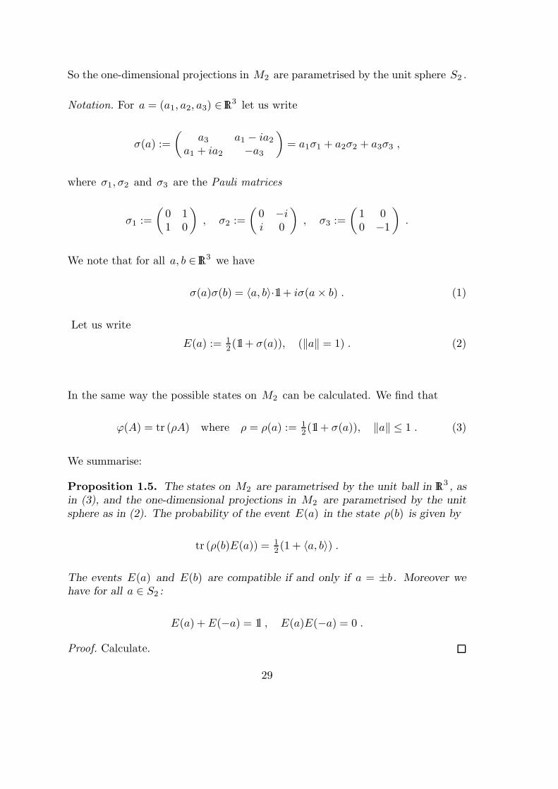
Notation. For a = (a1, a2, a3) ∈ IR3 let us write

σ(a) :=

(a3 a1 − ia2

a1 + ia2 −a3

)= a1σ1 + a2σ2 + a3σ3 ,

where σ1, σ2 and σ3 are the Pauli matrices

σ1 :=

(0 11 0

), σ2 :=

(0 −ii 0

), σ3 :=

(1 00 −1

).

We note that for all a, b ∈ IR3 we have

σ(a)σ(b) = 〈a, b〉·1l + iσ(a× b) . (1)

Let us write

E(a) := 12 (1l + σ(a)), (‖a‖ = 1) . (2)

In the same way the possible states on M2 can be calculated. We find that

ϕ(A) = tr (ρA) where ρ = ρ(a) := 12(1l + σ(a)), ‖a‖ ≤ 1 . (3)

We summarise:

Proposition 1.5. The states on M2 are parametrised by the unit ball in IR3 , asin (3), and the one-dimensional projections in M2 are parametrised by the unitsphere as in (2). The probability of the event E(a) in the state ρ(b) is given by

tr (ρ(b)E(a)) = 12 (1 + 〈a, b〉) .

The events E(a) and E(b) are compatible if and only if a = ±b . Moreover wehave for all a ∈ S2 :

E(a) + E(−a) = 1l , E(a)E(−a) = 0 .

Proof. Calculate.

29

Interpretation. The state of the qubit is given by a vector b in the three-dimensionalunit ball. For every a on the unit sphere we can say with probability one that ofthe two events E(a) and E(−a) exactly one will occur, E(a) having probability12(1 + 〈a, b〉). So we have a classical coin toss (with probability for heads equal to

12 (1 + 〈a, b〉)) for every direction in IR3 . The coin tosses in different directions areincompatible. (See Fig. 5.)Particular case: the ‘quantum fair coin’ is modelled by (M2,

12tr ).

The quantum coin toss is realised in nature: the spin direction of a particle withtotal spin 1

2 behaves in this way.

PhotonsThere is a second natural way to parametrise the one-dimensional projections inM2 , which is closer to the description of polarisation of photons.A one-dimensional projection corresponds to a (complex) line in C 2 , and such aline can be characterised by its slope, a number z ∈ C ∪ ∞ .

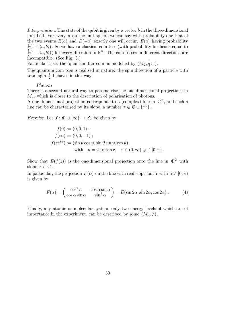
Exercise. Let f : C ∪ ∞ → S2 be given by

f(0) := (0, 0, 1) ;

f(∞) := (0, 0,−1) ;

f(reiϕ) := (sinϑ cosϕ, sinϑ sinϕ, cosϑ)

with ϑ = 2 arctan r, r ∈ (0,∞), ϕ ∈ [0, π) .

Show that E(f(z)) is the one-dimensional projection onto the line in C 2 withslope z ∈ C .

In particular, the projection F (α) on the line with real slope tanα with α ∈ [0, π)is given by

F (α) =

(cos2 α cosα sinα

cosα sinα sin2 α

)= E(sin 2α, sin 2α, cos 2α) . (4)

Finally, any atomic or molecular system, only two energy levels of which are ofimportance in the experiment, can be described by some (M2, ϕ).

30

4. Operations on probability spaces

‘The entire theory of probability isnothing but transforming variables.’

N.G. van Kampen

Our main objects of study will be operations on probability spaces. This meansthat we shall focus attention on the input-output aspect of probabilistic systems.

4.1 Operations on classical probability spaces

It could be maintained that operations are already the core of classical probability.We start with a definition on the level of points.

Definition. By an operation from a finite classical probability space Ω to a finiteclassical probability space Ω′ we mean an Ω×Ω′ transition matrix, i.e. a matrix(tωω′) of nonnegative numbers satisfying

∀ω∈Ω :∑

ω′∈Ω′

tωω′ = 1 .

Examples.1. Let τ be a bijection Ω → Ω′ . We may think of shuffling a deck of cards,

(Ω = Ω′ = cards), or the time evolution of a mechanical system (Ω = Ω′ =phase space), or the shift on sequences of letters, or just some relabeling ofthe outcomes of a statistical experiment. The associated matrix is

tωω′ :=

1 if ω′ = τ(ω),0 otherwise.

2. Let X : Ω → Ω′ be surjective. We think of X as an Ω′ -valued random

variable, where Ω′ is usually some subset of IR or IRn or so. The associatedoperation is that of ‘measuring X ’ or ‘forgetting everything about ω exceptthe value of X ’. The associated matrix is again

tωω′ :=

1 if ω′ = X(ω),0 otherwise.

3. An inverse to the operation of Example 2 is given by

tω′ω :=

π(ω)

π(X−1(ω′)) if ω′ = X(ω),

0 otherwise.

Here π is some probability distribution, which we assume to be everywherenonzero.

It can be shown that every transition matrix can be decomposed as a product ofmatrices of the types 3, 1 and 2. Such a decomposition is called a dilation of theoperation in question. See Section 4.3 for an example.

31

4.2 Operations on abelian *-algebras

All the above operations act on the points of Ω. In quantum probability, however,there are no such points. So in order to prepare for the introduction of quantumoperations, we reformulate the above examples into operations on ∗ -algebras andtheir duals, the spaces of probability distributions.

As before, we denote by C(Ω) the ∗ -algebra of complex functions on Ω. By C(Ω)∗

we shall mean the affine space of all probability distributions (πω)ω∈Ω on Ω, whichact on functions by the natural action

π(f) :=∑

ω∈Ω

π(ω)f(ω) .

Then an operation has a contravariant action T on the algebra and a covariantaction T ∗ on the dual as follows:

T : C(Ω′)→ C(Ω) : (Tf ′)(ω) :=∑

ω′∈Ω′

tωω′f ′(ω′) ;

T ∗ : C(Ω)∗ → C(Ω′)∗ : (T ∗π)(ω′) :=∑

ω∈Ω

π(ω)tωω′.

They are related by

∀π∈C(Ω)∗∀f ′∈C(Ω′) : π(Tf ′) =∑

ω∈Ω

∑

ω′∈Ω′

π(ω)tωω′f ′(ω′) = (T ∗π)(f ′) .

In fact, we shall be a bit sloppy, and sometimes denote by C(Ω)∗ the whole dualspace of C(Ω), not just the positive normalized functons.

Now we run through the examples again. Let us call C(Ω) : A and C(Ω′) : A′ .

1. Here T is a ∗ -isomorphism A′ → A , and T ∗ its dual action A′ → A . Everyinvertible operation is a ∗ -isomorphism. (Check!)

2. Let us denote the operation A′ → A associated to a random variable X byjX :

jX(f ′) := f ′ X .

Then jX is an injective ∗ -homomorphism:

jX(fg) = jX(f)jX(g); jX(f∗) = jX(f)∗ .

Every injective ∗ -homomorphism j : A′ → A is of the form jX for somerandom variable X . In quantum probability, random variables will be definedas ∗ -homomorphisms. This is the contravariant version or the Heisenberg

32

picture of a random variable, whereas the covariant version or the Schrodingerpicture of a random variable is

j∗X : π 7→ π X−1 .

Both describe the operation of restricting attention from ω to the values ω′

of X .

3. The operation jX : A′ → A above has left inverses: operations EπX : A → A′

of conditional expectation with respect to X and some probability distributionπ ∈ C(Ω)∗ :

EπX jX = id A′ .

In probability theory this conditional expectation of a function f ∈ C(Ω) isusually denoted as IE(f |X), where the dependence on the probability distri-bution π is implicit. We shall see below that a conditional expectation canbe defined as a right-invertible operation. The dual (EπX)∗ is the operation ofstochastic immersion or state extension of a distribution on Ω′ to a distribu-tion on the larger space Ω.

Let us now give the algebraic definition of an operation.Definition. By an operation from Ω to Ω′ we mean an affine map T ∗ takingprobability distributions on Ω to probability distributions on Ω′ . Such a map canbe extended to a linear map C(Ω)∗ → C(Ω′)∗ , which we shall denote by the samename T ∗ . Then T ∗ is a positive map (i.e. f ≥ 0 =⇒ Tf ≥ 0), which preservesnormalisation: ∑

ω′∈Ω′

(T ∗π)(ω′) =∑

ω∈Ω

π(ω) .

By duality an operation T ∗ brings with it a positive map

T : A′ → A with T1l′ = 1l .

We usually consider T and T ∗ as two descriptions of the same operation.

Theorem 4.1. Let (Ω, π) and (Ω′, π′) be finite classical probability spaces. Sup-pose that π(ω) > 0 for all ω ∈ Ω . Let j : C(Ω′) → C(Ω) and E : C(Ω) → C(Ω′)be operations such that

E j = id C(Ω′) and π′ E = π .

Then Ω has more points than Ω′ and there is a random variable X : Ω→ Ω′ suchthat

j = jX and E = EX .We first prove a lemma.

Lemma 4.2. (‘Abelian Schwartz’) For any positive 1l-preserving map T :C(Ω)→ C(Ω′) and all f ∈ C(Ω) we have:

T (|f |2) ≥ |Tf |2 .

33

Proof. For all λ, ϑ ∈ IR, f ∈ C(Ω):

0 ≤ T(|f − λeiϑ · 1l|2

)= T (|f |2)− 2λRe

(e−iϑTf

)+ λ2 .

So the quadratic function of λ which stands on the right can have at most onezero. Hence for all ϑ ∈ IR

T (|f |2) ≥(Re(eiϑTf

))2.

The statement follows.Proof of the Theorem. For all g ∈ C(Ω′):

|g|2 = E j(|g|2) ≥ E(|j(g)|2) ≥ |E j(g)|2 = |g|2 .So we have equality everywhere; it follows that

E(j(|g|2)− |j(g)|2

)= 0 .

Since π′ E = π :π(j(|g|2)− |j(g)|2

)= 0 .

But since j(|g|2) ≥ |j(g)|2 , and π is strictly positive everywhere, we have

j(|g|2) = |j(g)|2 .Now let hω := j(δω′). Then hω′ ≥ 0 and

h2ω′ = j(δω′)2 = j(δ2ω′) = j(δω′) = hω′ .

So hω′(ω) = 0 or 1 for all ω ∈ Ω, ω′ ∈ Ω′ . Moreover∑

ω′∈Ω′

hω′ =∑

ω′∈Ω′

j(δω′) = j(1l) = 1l .

Hence hω′ = 1S(ω′) for some partitionS(ω′)

∣∣ ω′ ∈ Ω′ of Ω. Define

X : Ω→ Ω′ : ω 7→ ω′ if ω ∈ S(ω′) .

Thenj(δω′)(ω) = 1S(ω′)(ω) = δω′(X(ω)) = jX(δω′)(ω) .

It follows that j = jX .Finally, let (eω′ω) denote the transition matrix of E : C(Ω) → C(Ω′). Then wehave for all ω′, ν′ ∈ Ω′ :

∑

ω∈S(ν′)

eω′ω =(E1S(ν′)

)(ω′) = E j(δν′)(ω′) = δν′(ω′) .

Hence eω′ω can only be nonzero if ω ∈ S(ω′), i.e. if ω′ = X(ω). And if the latteris the case, then

π′(ω′)eω′ω =∑

ν′∈Ω′

π′(ν′)eν′ω = (π′ E)(ω) = π(ω) .

Summarising we can conclude that

eω′ω =

π(ω)π′(ω′)

if ω′ = X(ω);

0 otherwise.

So E = EX . (See Example 3 of Subsection 4.1.)

34

4.3 A dilation

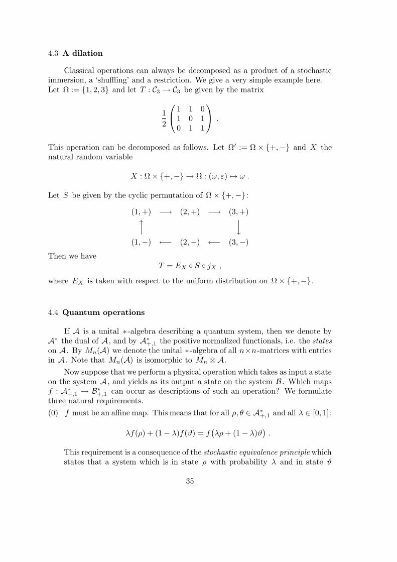
Classical operations can always be decomposed as a product of a stochasticimmersion, a ‘shuffling’ and a restriction. We give a very simple example here.Let Ω := 1, 2, 3 and let T : C3 → C3 be given by the matrix

1

2

1 1 01 0 10 1 1

.

This operation can be decomposed as follows. Let Ω′ := Ω× +,− and X thenatural random variable

X : Ω× +,− → Ω : (ω, ε) 7→ ω .

Let S be given by the cyclic permutation of Ω× +,− :

(1,+) −→ (2,+) −→ (3,+)x

y(1,−) ←− (2,−) ←− (3,−)

Then we haveT = EX S jX ,

where EX is taken with respect to the uniform distribution on Ω× +,− .

4.4 Quantum operations

If A is a unital ∗ -algebra describing a quantum system, then we denote byA∗ the dual of A , and by A∗

+,1 the positive normalized functionals, i.e. the stateson A . By Mn(A) we denote the unital ∗ -algebra of all n×n -matrices with entriesin A . Note that Mn(A) is isomorphic to Mn ⊗A .

Now suppose that we perform a physical operation which takes as input a stateon the system A , and yields as its output a state on the system B . Which mapsf : A∗

+,1 → B∗+,1 can occur as descriptions of such an operation? We formulatethree natural requirements.

(0) f must be an affine map. This means that for all ρ, θ ∈ A∗+,1 and all λ ∈ [0, 1]:

λf(ρ) + (1− λ)f(ϑ) = f(λρ+ (1− λ)ϑ

).

This requirement is a consequence of the stochastic equivalence principle whichstates that a system which is in state ρ with probability λ and in state ϑ

35

with probability 1 − λ can not be distinguished from a system in the stateλρ+ (1− λ)ϑ .

A map f satisfying (0) can be extended to a unique linear map A∗ → B∗ , sinceevery element of A∗ can be written as a linear combination of (at most four)states on A . So f must be the adjoint of some linear map T : B → A . We shallhenceforth write T ∗ instead of f . Of course, T ∗ must still map A∗

+,1 to B∗+,1 :

(1) tr (T ∗ρ) = tr (ρ) for all ρ ∈ A∗ ;If ρ ≥ 0 then also T ∗ρ ≥ 0.

It would seem at first sight that nothing more can be said a priori about T ∗ .However, it was realised in the early 1970’s by Karl Kraus that the positivityproperty has to be strengthened in quantum mechanics: if our main system is ina combined state with some other system, then after performing the operation T ∗

on the main system, the whole combination must still be in some (positive) state.Surprisingly, this is not automatic in the quantum situation, where ‘entanglement’,as treated in Chapter 1, between the main system and the second system is pos-sible. See Example 4.3 below.Therefore this stronger form of positivity must be added as a requirement.

(2) For all n ∈ IN the map id n⊗T ∗ maps states on Mn⊗A to states on Mn⊗B .

Requirement (2) is called complete positivity of the map T ∗ (or T for that matter).

Summarizing we arrive at the following definition, which we shall formulate in thecontravariant, ‘Heisenberg’ picture.

Definition. A linear map T : B → A is called an operation (from A to B !) ifthe following conditions hold:

(1) T (1lB) = 1lA ;

(2) T is completely positive, i.e. id n ⊗ T is positive Mn(B) → Mn(A) for alln ∈ IN.

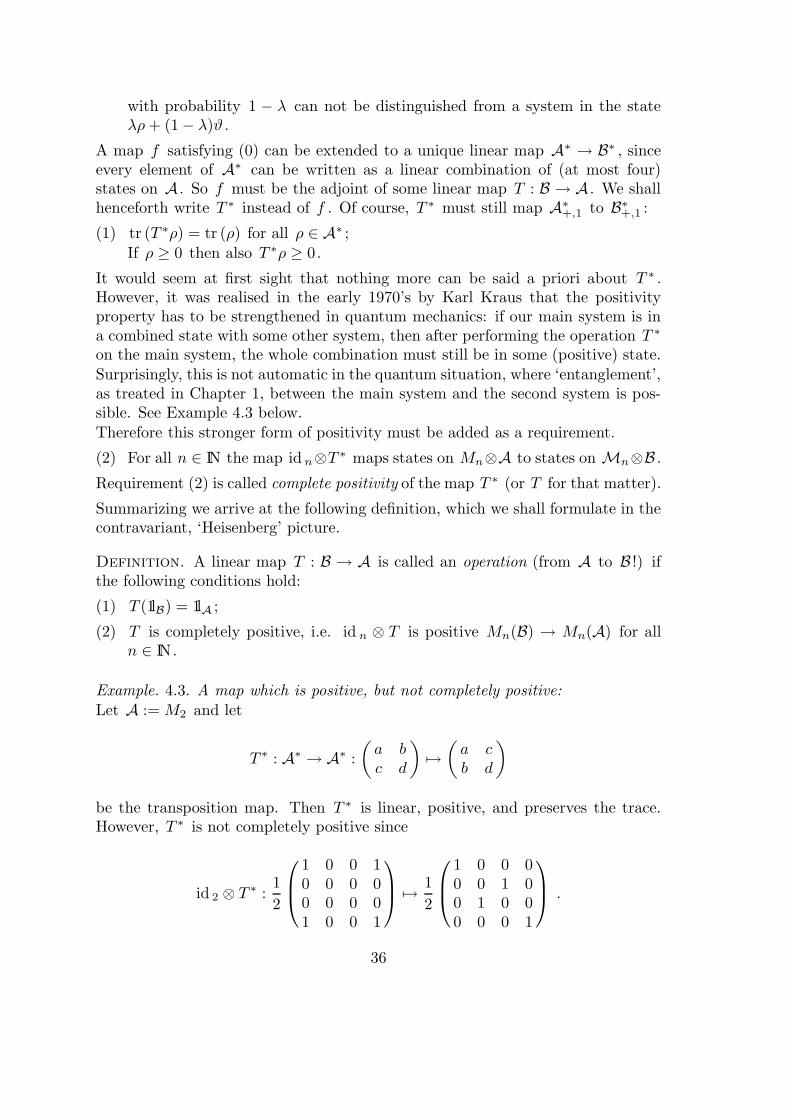
Example. 4.3. A map which is positive, but not completely positive:Let A := M2 and let

T ∗ : A∗ → A∗ :

(a bc d

)7→(a cb d

)

be the transposition map. Then T ∗ is linear, positive, and preserves the trace.However, T ∗ is not completely positive since

id 2 ⊗ T ∗ :1

2

1 0 0 10 0 0 00 0 0 01 0 0 1

7→ 1

2

1 0 0 00 0 1 00 1 0 00 0 0 1

.

36

The matrix on the left is a projection (on the vector (e0 ⊗ e0 + e1 ⊗ e1)/√

2 ∈C2⊗ C2 ; compare the entangled state of Section 2.5.); whereas the matrix on theleft has eigenvalues 1

2 ,12 ,

12 and − 1

2 , hence is not a valid density matrix.

However, if A or B is abelian, then any positive operator T : A → B is automat-ically completely positive. (We state this without proof.)

Examples. 4.4. Some quantum operations

1. Let U ∈Mn be unitary. Then the automorphism T : Mn →Mn : A 7→ U∗AUis an operation. (See Lemma 1 below.)

2. The ∗ -homomorphism j : Mk →Ml ⊗Mk : A 7→ 1l⊗A is an operation. (SeeLemma 1 below.)

3. Let ϕ be a state on Mk . Then the map E : Ml⊗Mk →Mk : B⊗A 7→ ϕ(B)Ais an operation.

The above examples are to be compared with those in Section 4.1.

Lemma 4.5. If A ⊂ Mk and T : A → B ⊂ Ml is a ∗-homomorphism, i.e. iffor all A , B ∈ A we have T (AB) = T (A)T (B) and T (A∗) = T (A)∗ , then T iscompletely positive.

Proof. We must show that for all n ∈ IN the map

id n ⊗ T :(Aij)ni,j=1

7→(T (Aij)

)ni,j=1

is positive. Indeed, for all ψ = (ψ1, · · · , ψn) ∈ (C l)n , putting A = X∗X withX ∈Mn(A):

〈ψ, (id n ⊗ T )(X∗X)ψ〉 =l∑

i,i′=1

〈ψi, T((X∗X)ii′

)ψi′〉

=l∑

i,i′=1

n∑

j=1

〈ψi, T(X∗jiXji′

)ψi′〉

=l∑

i,i′=1

n∑

j=1

〈ψi, T (Xji)∗T (Xji′)ψi′〉

=n∑

j=1

‖T (Xji)ψi ‖2 ≥ 0 .

37

Lemma 4.6. Let A ⊂Mk , B ⊂Ml and let V be a linear map C l → Ck . Then

T : A → B : A 7→ V ∗AV

is completely positive.

Proof. If (Aij)ni,j=1 ∈ Mn(A) is positive, then for all (ψ1, · · · , ψn) ∈ (C l)n =

Cn ⊗ C l we have

〈ψ, (id n ⊗ T )(A)ψ〉 =n∑

i,j=1

〈ψi, T (Aij)ψj〉

=

n∑

i,j=1

〈ψi, V ∗AijV ψj〉

=n∑

i,j=1

〈V ψi, AijV ψj〉 ≥ 0 .

Lemma 2 covers Example 3 of 4.4. since ϕ can be decomposed into pure states asϕ =

∑i〈ψ, ·ψ〉 and

ϕ(B)A =l∑

i=1

λi〈ψi, Bψi〉A =l∑

i=1

λiV∗i (B ⊗A)Vi ,

where Vi : Ck → C l ⊗ Ck : ϑ 7→ ψi ⊗ ϑ .The following important theorem, together with Proposition 3.6, characterizes

all completely positive maps on finite dimensional ∗ -algebras.

Theorem 4.7. (Stinespring 1955). Let T be a linear map Mk → Ml . Thefollowing are equivalent.(i) T is completely positive;(ii) There exist m ∈ IN and operators V1, . . . Vm : C l → Ck such that for all

A ∈Mk :

T (A) =m∑

i=1

V ∗i AVi .

Moreover, if the matrices V1, . . . , Vm are linearly independent, then they are de-termined by the completely positive map T up to a transformation of the form

V ′i :=

m∑

j=1

uijVj ,

38

where (uij)mi,j=1 is a unitary m×m-matrix of complex numbers.

We begin with some preparatory work.

Proposition 4.8. Let ϕ be a state on A := Mk . Then any two decomposi-tions of ϕ into m pure states

ϕ(A) =

m∑

i=1

〈ψi, Aψi〉 =m∑

i=1

〈ϑi, Aϑi〉 (5)

with linearly independent vectors ψ1, . . . , ψm , are connected by a transformationof the form

ϑi =m∑

j=1

uijψj .

where (uij)mi,j=1 ∈Mm .

Proof. Consider ψ := (ψ1, . . . , ψm) and ϑ := (ϑ1, . . . , ϑm) as vectors in H :=(Ck)m = Cm ⊗ Ck . Then (5) can be written in the form

ϕ(A) = 〈ψ, (1l⊗ A)ψ〉 = 〈ϑ, (1l⊗ A)ϑ〉 .

(So we see that any state can be written as a pure state on some representa-tion of A !) Now, since the vectors ψ1, . . . , ψm are independent, for any m -tuple (χ1, . . . , χm) ∈ H there exists a matrix A ∈ A such that for all i wehave Aψi = χi . In other words: H = (1l⊗A)ψ . Now define U : H → H by:

U(1l⊗ A)ψ := (1l⊗A)ϑ .

Then U is isometric, since

‖U(1l⊗ A)ψ ‖2 = ‖ (1l⊗ A)ϑ ‖2 = 〈(1l⊗ A)ϑ, (1l⊗A)ϑ〉 = 〈ϑ, (1l⊗ A∗A)ϑ〉= ϕ(A∗A) = ‖ (1l⊗ A)ψ ‖2 ,

and since U maps H into H itself, it must be unitary. What is more, U ∈Mm⊗Mk is actually of the form u⊗ 1l for some unitary u ∈Mm . Indeed, for allχ = (1l⊗X)ψ ∈ H and all A ∈ A we have

U(1l⊗A)χ = U(1l⊗ AX)ψ = (1l⊗ AX)ϑ = (1l⊗A)(1l⊗X)ϑ

= (1l⊗ A)U(1l⊗X)ψ = (1l⊗A)Uχ ,

and therefore U ∈ (1l⊗A)′ = Mm ⊗ 1l. The statement follows.

39

We shall now introduce some useful notation.Consider the tensor product Hkl := Ck ⊗ (C l)′ of the Hilbert space Ck and thedual of C l . Hkl can be viewed as the space of all operators C l → Ck , but alsoas a Hilbert space (with natural inner product), on which the algebra Mk ⊗MT

l

can act, in the following way:

A⊗B : ψ ⊗ ϑ 7→ Aψ ⊗ Bϑ[= A|ψ〉 ⊗ 〈ϑ|BT

].

The space Hll has a natural rotation invariant vector (the so-called fully entangledstate on Ml ⊗MT

l ), given by

Ω :=l∑

i=1

ei ⊗ ei[ l∑

i=1

|ei〉 ⊗ 〈ei|],

for any(!) orthonormal basis e1, . . . , el of C l . This vector has the property that

〈Ω, (A⊗ B)Ω〉H =l∑

i=1

l∑

j=1

〈ei ⊗ ei, (A⊗ B)ej ⊗ ej〉H

=

l∑

i=1

l∑

j=1

〈ei, Aej〉〈ei, Bej〉

=

l∑

i=1

l∑

j=1

〈ei, Aej〉〈ej , BT ei〉

= tr (ABT ) = tr (ATB) ,

(6)

where ·T denotes transposition.

Proof of Stinespring’s Theorem. The implication (ii)=⇒(i) follows immediatelyfrom Lemma 4.2. For the converse, assume that T : Mk → Ml is completelypositive. Let Hll := C l ⊗ (C l)′ as above, and let ω denote the state

ω(X) := 〈Ω, XΩ〉

on B(Hll) ∼ Ml ⊗ Ml . Since T is completely positive, the functional ωT onB(Hkl) given by

ωT := (T ∗ ⊗ id )(ω)

is also a state. Decompose ωT into pure states given by vectors v1, v2, . . . , vm ∈Hkl :

ωT (X) =m∑

i=1

〈vi, Xvi〉 .

40

Now, vi ∈ Hkl can be considered as an operator Vi : C l → Ck . We shall showthat these operators satisfy the requirement (ii) in the theorem. Indeed, for allψ, ϑ ∈ C l :

m∑

i=1

〈ψ, V ∗i AViϑ〉 =

m∑

i=1

〈Viψ,AViϑ〉

=

m∑

i=1

〈vi,(A⊗ (ψ ⊗ ϑ)

)vi〉H

= ωT(A⊗ (ψ ⊗ ϑ)

)

= ω(T (A)⊗ (ψ ⊗ ϑ)

)

= 〈Ω, T (A)⊗ (ψ ⊗ ϑ)Ω〉= tr

(T (A)(ϑ⊗ ψ)

)

= 〈ψ, T (A)ϑ〉 .

When A and B are operators on a Hilbert space, we mean by A ≥ B that thedifference A − B is a positive operator. The following is an extremely usefulinequality for operations.

Proposition 4.9. (Cauchy-Schwarz for operations) Let A and B be *-algebras of operators on Hilbert spaces H and K , and let T : A → B be anoperation. Then we have for all A ∈ A :

T (A∗A) ≥ T (A)∗T (A) .

Proof. The operator X ∈M2 ⊗A given by

X :=

(A∗A −A∗

−A 1l

)=

(A −1l0 0

)∗(A −1l0 0

)

is positive. Since T is completely positive and T (1l) = 1l, it follows that also

(id ⊗ T )(X) =

(T (A∗A) −T (A)∗

−T (A) 1l

)

is a positive operator. Putting ξ := ψ ⊕ T (A)ψ we find that

〈ξ, (id ⊗ T )Xξ〉 = 〈ψ,(T (A∗A)− T (A)∗T (A)

)ψ〉

is positive for all ψ ∈ H .

41

Theorem 4.10. (Multiplication Theorem) If T : A → B is an operation andT (A∗A) = T (A)∗T (A) for some A ∈ A , then T (A∗B) = T (A)∗T (B) andT (B∗A) = T (B)∗T (A) for all B ∈ A .

Proof. Take any B ∈ A and λ ∈ IR. Then

T((A∗ + λB∗)(A+ λB)

)= T (A)∗T (A) + λT (A∗B + B∗A) + λ2T (B∗B) ,

while by Cauchy-Schwartz

T((A∗ + λB∗)(A+ λB)

)

≥ T (A)∗T (A) + λ(T (A)∗T (B) + T (B)∗T (A)) + λ2T (B)∗T (B)) .

This inequality holds for all λ ∈ R which implies

T (A∗B +B∗A) ≥ T (A)∗T (B) + T (B)∗T (A) .

Replacing A by iA and B by −iB shows that the opposite inequality also holds,so we have equality. Finally replacing only B by iB shows that T (A∗B) =T (A)∗T (B) and T (B∗A) = T (B)∗T (A).

In particular, if a Schwartz equality holds for an operation T then T is a *-homomorphism.

Theorem 4.11. (Embedding theorem) Let (A, ϕ) and (B, ψ) be nondegeneratequantum probabality spaces, and let j : A → B , E : B → A be operations whichpreserve the states. If

E j = id A ,

then j is an injective *-homomorphism and P := jE is a conditional expectation,i.e.,

P (C1BC2) = C1P (B)C2 (7)

for all C1, C2 ∈ j(A) and all B ∈ B .

Following the language used in Section 4.1. we shall call j a random variable andP the conditional expectation with respect to ψ , given j . Compare the followingproof with that of Theorem 4.1.

Proof. For any A ∈ A we have by Cauchy-Schwartz

A∗A = E j(A∗A) ≥ E(j(A)∗j(A)) ≥ E j(A)∗E j(A) = A∗A , (8)

so we have equalities here. In particular

ψ(j(A∗A)− j(A)∗j(A)

)= ϕ E

(j(A∗A)− j(A)∗j(A)

)= 0 ,

42

and as (B, ψ) is non-degenerate, j(A∗A) = j(A)∗j(A), i.e. j is a *-homomorphism.j is injective since it has the left-inverse E .But also from (8) we have E

(j(A)∗j(A)

)= E j(A)∗E j(A). The Multiplication

Theorem 4.10 then implies that for all B ∈ B and A1 ∈ A ,

E(j(A1)∗B) = E j(A1)

∗E(B) = A∗1E(B) ,

and similarly, with A2 ∈ A :

E(j(A1)

∗Bj(A2))

= E(j(A1)

∗B)E j(A2) = A∗

1E(B)A2 .

Applying j to both sides we find (7).

5. Quantum impossibilities

The result of any physical operation applied on a probabilistic system (quan-tum or not) is described by a completely positive identity preserving map fromthe state space of that system to the state space of the resulting system. Thisimposes strong restrictions on what can be done. Some of these are well-knownquantum principles, such as the Heisenberg principle (‘no measurement withoutdisturbance’), some are surprising and relatively recent discoveries (‘no cloning’),but all of them obtain quite neat formulations in the language of quantum prob-ability.

5.1 ‘No cloning’

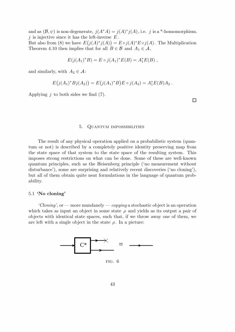
‘Cloning’, or — more mundanely — copying a stochastic object is an operationwhich takes as input an object in some state ρ and yields as its output a pair ofobjects with identical state spaces, such that, if we throw away one of them, weare left with a single object in the state ρ . In a picture:

=C*

fig. 6

43

In a formula: for all ρ ∈ A∗+,1 :

(tr ⊗ id ) C∗(ρ) = (id ⊗ tr ) C∗(ρ) = ρ . (9)

Reformulated in the Heisenberg picture: for all A ∈ A :

C(1l⊗A) = C(A⊗ 1l) = A . (10)

As is well known, copying presents no problem in classical physics, or classicalprobability. Here is an example of a classical copying operation. For simplicity,let us think of the operation of copying n bits. Let Ω denote the space 0, 1nof all strings of n bits, and let γ be the ‘copying’ map Ω → Ω× Ω : ω 7→ (ω, ω).This map induces an operation

C : C(Ω)× C(Ω)→ C(Ω) : Cf(ω) := f γ(ω) = f(ω, ω) .

Clearly, for all f ∈ C(Ω):

C(1l⊗ f)(ω) = (1l⊗ f)(ω, ω) = f(ω) ,

and the same holds for C(f ⊗ 1l), so (10) is satisfied. In the Schrodinger pictureour operation looks as follows:

(C∗π)(ν, ω) = δνωπ(ω) ,

and we see that (9) is satisfied:

(tr ⊗ id ) C∗(π)(ω) =∑

ν∈Ω

δνωπ(ω) = π(ω) .

The following theorem says that this construction is only possible in the abeliancase.

Theorem 5.1. (‘No cloning’) Let C : A ⊗ A → A be an operation. If equation(10) holds for all A ∈ A , then A is abelian.

Proof. (10) implies that for all A ∈ A :

C((1l⊗ A)∗(1l⊗ A)

)= C(1l⊗A∗A) = A∗A = C(1l⊗A)∗C(1l⊗ A)

Then it follows from the multiplication theorem that for all A,B ∈ A :

AB = C(A⊗ 1l)C(1l⊗ B) = C((A⊗ 1l)(1l⊗ B)

)

= C((1l⊗ B)(A⊗ 1l)

)= C(1l⊗ B)C(A⊗ 1l) = BA .

44

5.2 ‘No classical coding’

Closely related to the above is the rule that ‘quantum information cannot beclassically coded’: It is not possible to operate on a quantum system, extractingsome information from it, and then from this information reconstruct the quantumsystem in its original state:

ρ ∈ A∗ C∗

7−→π ∈ B∗ D∗

7−→ ρ ∈ A∗ .

We formulate this theorem in the contravariant (‘Heisenberg’) picture:

Theorem 5.2. Let A and B be *-algebras, and let C : B → A and D : A → Bbe operations, (‘Coding’ and ‘Decoding’), such that C D = id A . Then if B isabelian, so is A .Proof. We have for all A ∈ A :

A∗A = C D(A∗A) ≥ C(D(A)∗D(A)

)≥ A∗A

and AA∗ = C D(AA∗) ≥ C(D(A)D(A)∗

)≥ AA∗ ,

so that we again have equality everywhere. If B is abelian, we have D(A)∗D(A) =D(A)D(A)∗ , so that A∗A = AA∗ .

Exercise. Prove that, if A∗A = AA∗ for all A ∈ A , then A is abelian.

5.3 The Heisenberg Principle

The Heisenberg principle states — roughly speaking — that no informationon a quantum system can be obtained without changing its state.

In this form, the statement is not so interesting: if we realise that the state ofthe system expresses the expectations of its observables, given the information wehave on it, it is no wonder that this state changes once we gain information!A more precise formulation is the following:

If we extract information from a system whose algebra A is a factor (i.e.A ∩ A′ = C1l), and if we throw away (disregard) this information, thenit can not be avoided that some initial states are altered.

Let us work towards a mathematical formulation.A measurement is an operation performed on a physical system which results inthe extraction of information from that system, while possibly changing its state.So a measurement is an operation

M∗ : A∗ → A∗ ⊗ B∗ ,

where A describes the physical system, and B the output part of a measurementapparatus which we couple to it. A∗ consists of states and B∗ of probability

45

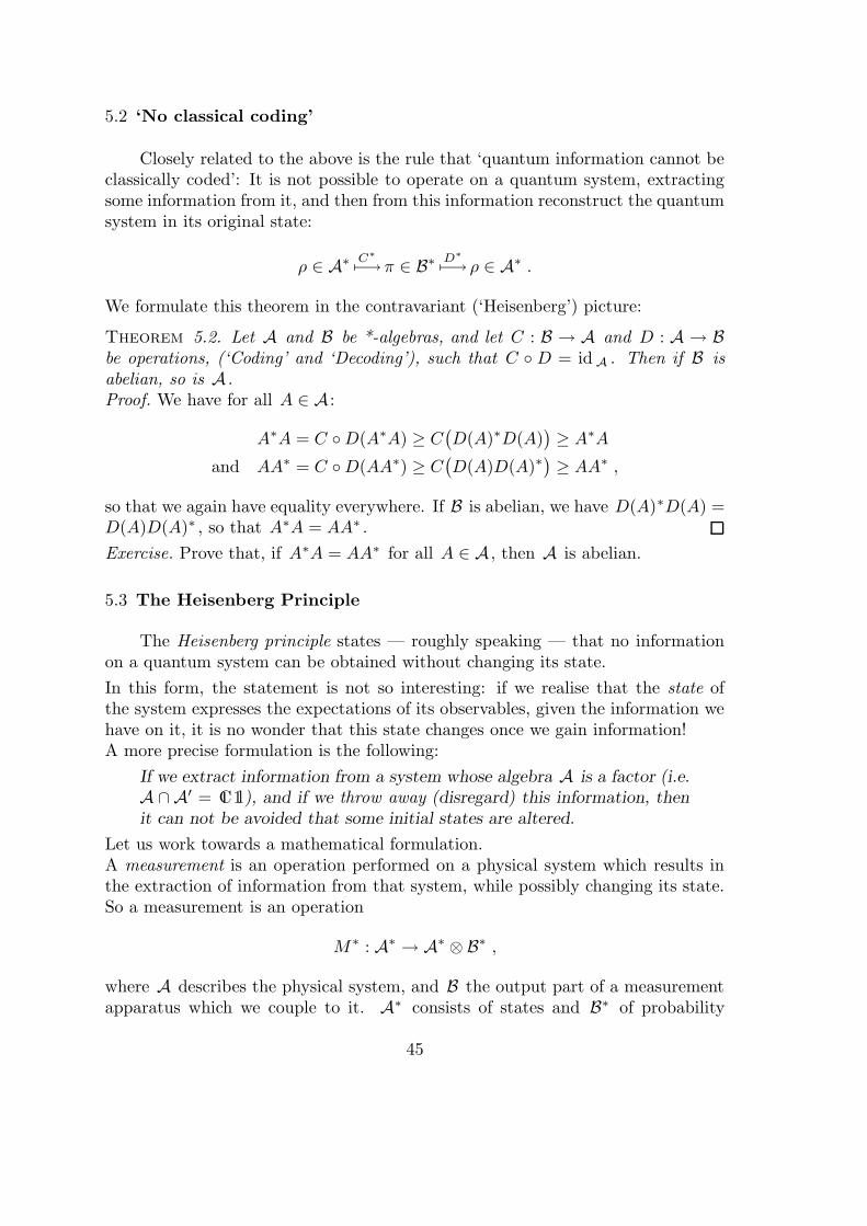
distributions on the outcomes. So B will be commutative, but we do not need thisproperty here.Now suppose that no initial state is altered by the measurement:

(id ⊗ tr )M∗(ρ) = ρ ∀ρ∈A∗ .

Suppose also that A is a factor. We claim that no information can be obtainedon ρ :

(tr ⊗ id )M∗(ρ) = ϑ ,

where ϑ does not depend on ρ .

In a picture:

M*

M*

=

=

fig. 7

We again formulate and prove the theorem in the contravariant picture:

Theorem 5.3. (Heisenberg’s Principle) Let M be an operation A⊗B → A suchthat for all A ∈ A ,

M(A⊗ 1l) = A ,

thenM(1l⊗B) ∈ A ∩ A′ .

In particular, if A is a factor, then B 7→M(1l⊗B) = ϑ(B) · 1lA for some state ϑon B .

Proof. As in the proof of the ‘no cloning’ theorem we have by the multiplicationtheorem for all A ∈ A , B ∈ B :

M(1l⊗ B) ·A = M(1l⊗B)M(A⊗ 1l) = M(A⊗ B) .

46

But also,A ·M(1l⊗ B) = M(A⊗ 1l)M(1l⊗ B) = M(A⊗ B) .

So M(1l⊗B) lies in the center of A . If A is a factor, then B 7→M(1l⊗B) is anoperation from B to C · 1lA , i.e. a state on B times 1lA .

5.4 Random variables and von Neumann measurements

Following the suggestion made in Section 4.2. (in particular case 2), we definea random variable to be a *-homomorphism from one algebra B to a (larger)algebra A :

A j←−B .In the covariant (‘Schrodinger’) picture this describes the operation j∗ of restric-tion to the subsystem B :

A∗ j∗−→B∗ .An important case is when B = C(Ω) for some finite set Ω: then j is to beviewed as an Ω-valued random variable. Let Ω = x1, . . . , xn . Then j(1xi) isa projection, Pi say, in A , with the properties that

n∑

i=1

Pi =n∑

i=1

j(1xi) = j(1lB) = 1lA

and for i 6= j ,

PiPk = j(1xi)j(1xk) = j(1xi · 1xk) = 0 .

We interpret Pi as the event ‘the random variable described by j takes the valuexi ’. Note that j can be written as

j(f) = j

(n∑

i=1

f(xi)1xi

)=

n∑

i=1

f(xi)Pi .

In particular, if Ω ⊂ IR, then j defines a hermitian operator

j(id ) =

n∑

i=1

xiPi =: X ,

which completely determines j .

Proposition 5.4. Let A be a finite-dimensional *-algebra with unit. Then thereis a one-to-one correnspondence between injective *-homomorphisms j : C(Ω)→ Afor some Ω ⊂ IR and self-adjoint operators X ∈ A , given by

j(id ) = X .

47

Proof. If j is a *-homomorphism C(x1, . . . , xn)→ A with x1, . . . , xn real, then

X := j(id ) =n∑

i=1

xij(1xi) =:n∑

i=1

xiPi

is a hermitian element of A . Conversely, if X ∈ A is hermitian, then let x1, . . . , xnbe its eigenvalues. Let p : C → C denote the polynomial

p(x) := (x− x1) · · · (x− xn) .

and let, for i = 1, . . . , n , the (Lagrange interpolation) polynomial pi be given by

pi(x) :=p(x)

(x− xi)p(xi).

Then pi(xk) = δikpk , so we have on the spectrum x1, . . . , xn of X :

n∑

i=1

pi = 1 and pi · pk = δikpk .

It follows that the projections Pi := pi(X), with i = 1, . . . , n , lie in the algebraA and satisfy

n∑

i=1

Pi = 1l and PiPk = δikPk .

Hence, if we define

j(f) :=

n∑

i=1

f(xi)Pi ,

then j is a *-homomorphism with the property that j(id ) = X . Clearly, differentX ’s correspond to different j ’s.

5.5 The joint measurement apparatus

Let X and Y be self-adjoint elements of the *-algebra A . We consider Xand Y as random variables taking values in the spectra sp(X) and sp(Y ).By a joint measurement M∗ of these random variables we mean an operationthat takes a state ρ on A as input, and yields a probability distribution π onsp(X)× sp(Y ) as output, in such a way that for all functions f on sp(X), g onsp(Y ):

ρ(f(X)) =∑

x∈sp(X)

∑

y∈sp(Y )

π(x, y)f(x) ;

ρ(g(Y )) =∑

x∈sp(X)

∑

y∈sp(Y )

π(x, y)g(y) .

48

A contravariant formulation of these facts is

M(f ⊗ 1l) = f(X) ;

M(1l⊗ g) = g(Y ) .

Theorem 5.5. If two random variables X and Y allow a joint measurementoperation, then they commute.

Proof. Let us denote by x the identity function on sp(X), and by y that on sp(Y ).We apply the multiplication theorem on the measurement operation M , which issupposed to exist. Since

M((x⊗ 1l)∗(x⊗ 1l)

)= M(x2 ⊗ 1l) = X2 = M(x⊗ 1l)∗M(x⊗ 1l) ,

we haveM((x⊗ 1l)∗(1l⊗ y)

)= M(x⊗ 1l)∗M(1l⊗ y) = XY

andM((1l⊗ y)∗(x⊗ 1l)

)= M(1l⊗ y)∗M(x⊗ 1l) = Y X .

As (x⊗ 1l)∗(1l⊗ y) = x⊗ y = (1l⊗ y)∗(x⊗ 1l), we have XY = Y X .

6. Quantum novelties

In the previous chapter we saw certain strange limitations that quantum oper-ations are subject to. Let us now look at the other side of the coin: some surprisingpossibilities.We leave treatment of the really sensational features to later chapters, such as veryfast computation and secure cryptography. Here we shall treat ‘teleportation’ ofquantum states and ‘superdense coding’.

6.1 Teleportation of quantum states

Suppose that Alice wishes to send to Bob the quantum state ρ of a qubit overa (classical) telephone line.In Section 5.2 (‘No classical coding’) we have seen that, without any further tools,this is impossible. If Alice were to perform measurements on the qubit, and tellthe results to Bob over the telephone, these would not enable Bob to reconstructthe state ρ .However, suppose that Alice and Bob have been together in the past, and that atthat time they have created an entangled pair of qubits, as introduced in Section1.3, taking one qubit each home with them.

49

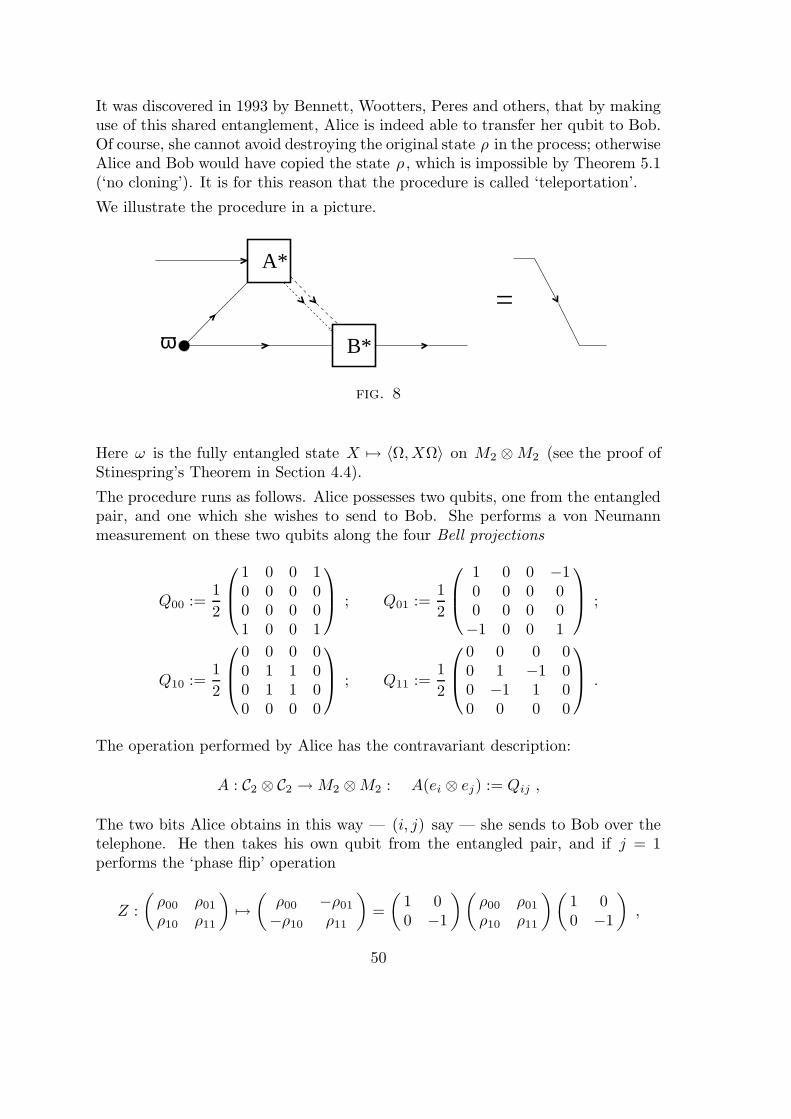
It was discovered in 1993 by Bennett, Wootters, Peres and others, that by makinguse of this shared entanglement, Alice is indeed able to transfer her qubit to Bob.Of course, she cannot avoid destroying the original state ρ in the process; otherwiseAlice and Bob would have copied the state ρ , which is impossible by Theorem 5.1(‘no cloning’). It is for this reason that the procedure is called ‘teleportation’.

We illustrate the procedure in a picture.

=A*

B*ω

fig. 8

Here ω is the fully entangled state X 7→ 〈Ω, XΩ〉 on M2 ⊗M2 (see the proof ofStinespring’s Theorem in Section 4.4).

The procedure runs as follows. Alice possesses two qubits, one from the entangledpair, and one which she wishes to send to Bob. She performs a von Neumannmeasurement on these two qubits along the four Bell projections

Q00 :=1

2

1 0 0 10 0 0 00 0 0 01 0 0 1

; Q01 :=

1

2

1 0 0 −10 0 0 00 0 0 0−1 0 0 1

;

Q10 :=1

2

0 0 0 00 1 1 00 1 1 00 0 0 0

; Q11 :=

1

2

0 0 0 00 1 −1 00 −1 1 00 0 0 0

.

The operation performed by Alice has the contravariant description:

A : C2 ⊗ C2 →M2 ⊗M2 : A(ei ⊗ ej) := Qij ,

The two bits Alice obtains in this way — (i, j) say — she sends to Bob over thetelephone. He then takes his own qubit from the entangled pair, and if j = 1performs the ‘phase flip’ operation

Z :

(ρ00 ρ01

ρ10 ρ11

)7→(ρ00 −ρ01

−ρ10 ρ11

)=

(1 00 −1

)(ρ00 ρ01

ρ10 ρ11

)(1 00 −1

),

50

and if j = 0 he does nothing. Then, if i = 1 he performs the ‘quantum not’operation

X :

(ρ00 ρ01

ρ10 ρ11

)7→(ρ11 ρ10

ρ01 ρ00

)=

(0 11 0

)(ρ00 ρ01

ρ10 ρ11

)(0 11 0

),

and if i = 0 he does nothing. In the Heisenberg picture, the result of Bob’s actionsis the operation

B : M2 → C2 ⊗ C2 ⊗M2 : M 7→M ⊕ σ3Mσ3 ⊕ σ1Mσ1 ⊕ σ2Mσ2 ,

where σ1 :=

(0 11 0

), σ2 :=

(0 −ii 0

), and σ3 :=

(1 00 −1

), are Pauli’s spin

matrices. Bob ends up with a qubit in exactly the same state as Alice wanted tosend.We formulate this result in the Heisenberg picture.

Proposition 6.1. The state ω and the operations A and B described abovesatisfy

(idM2⊗ ω) (A⊗ idM2

) B = idM2.

Proof. We just calculate for M ∈M2 :

MB7−→M ⊕ σ3Mσ3 ⊕ σ1Mσ1 ⊕ σ2Mσ2

A⊗id7−→ (Q00 ⊗M) + (Q01 ⊗ σ3Mσ3) + (Q10 ⊗ σ1Mσ1) + (Q11 ⊗ σ2Mσ2)

=1

2

M + σ3Mσ3 0 0 M − σ3Mσ3

0 σ1Mσ1 + σ2Mσ2 σ1Mσ1 − σ2Mσ2 00 σ1Mσ1 − σ2Mσ2 σ1Mσ1 + σ2Mσ2 0

M − σ3Mσ3 0 0 M + σ3Mσ3

=

m00 0 0 0 | 0 0 0 m01

0 m11 0 0 | 0 0 m10 00 0 m11 0 | 0 m01 0 00 0 0 m00 | m01 0 0 0− − − − | − − − −0 0 0 m10 | m11 0 0 00 0 m01 0 | 0 m00 0 00 m01 0 0 | 0 0 m00 0m10 0 0 0 | 0 0 0 m11

id⊗ω7−→(m00 m01

m10 m11

)= M .

51

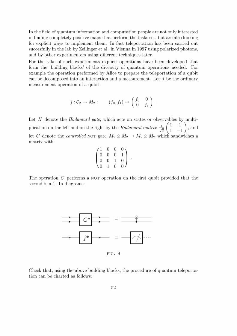
In the field of quantum information and computation people are not only interestedin finding completely positive maps that perform the tasks set, but are also lookingfor explicit ways to implement them. In fact teleportation has been carried outsuccesfully in the lab by Zeilinger et al. in Vienna in 1997 using polarized photons,and by other experimenters using different techniques later.

For the sake of such experiments explicit operations have been developed thatform the ‘building blocks’ of the diversity of quantum operations needed. Forexample the operation performed by Alice to prepare the teleportation of a qubitcan be decomposed into an interaction and a measurement. Let j be the ordinarymeasurement operation of a qubit:

j : C2 →M2 : (f0, f1) 7→(f0 00 f1

).

Let H denote the Hadamard gate, which acts on states or observables by multi-

plication on the left and on the right by the Hadamard matrix 1√2

(1 11 −1

), and

let C denote the controlled not gate M2 ⊗M2 → M2 ⊗M2 which sandwiches amatrix with

1 0 0 00 0 0 10 0 1 00 1 0 0

.

The operation C performs a not operation on the first qubit provided that thesecond is a 1. In diagrams:

=

=

C*

j*

fig. 9

Check that, using the above building blocks, the procedure of quantum teleporta-tion can be charted as follows:

52

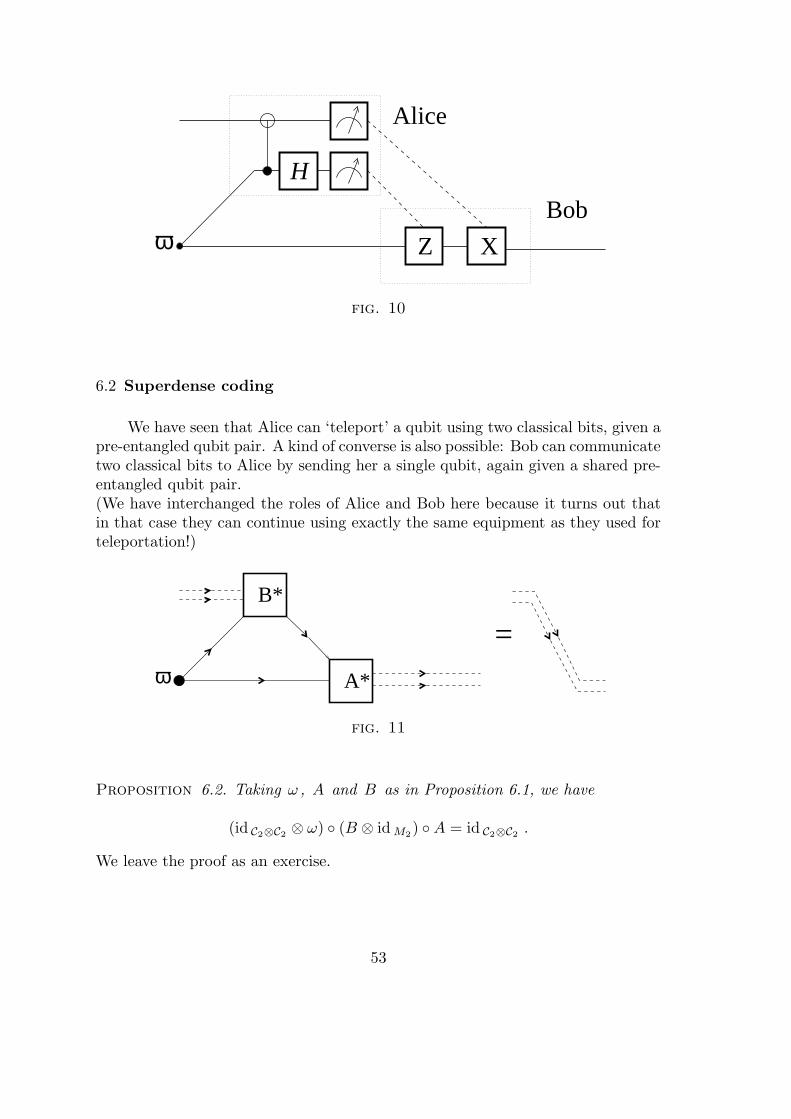
Alice

Bob

XZ

H

ω

fig. 10

6.2 Superdense coding

We have seen that Alice can ‘teleport’ a qubit using two classical bits, given apre-entangled qubit pair. A kind of converse is also possible: Bob can communicatetwo classical bits to Alice by sending her a single qubit, again given a shared pre-entangled qubit pair.(We have interchanged the roles of Alice and Bob here because it turns out thatin that case they can continue using exactly the same equipment as they used forteleportation!)

=B*

A*ω

fig. 11

Proposition 6.2. Taking ω , A and B as in Proposition 6.1, we have

(id C2⊗C2⊗ ω) (B ⊗ idM2

) A = id C2⊗C2.

We leave the proof as an exercise.

53

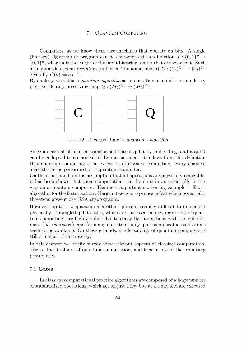
7. Quantum Computing

Computers, as we know them, are machines that operate on bits. A single(finitary) algorithm or program can be characterised as a function f : 0, 1p →0, 1q , where p is the length of the input bitstring, and q that of the output. Sucha function defines an operation (in fact a *-homomorphism) C : (C2)⊗q → (C2)⊗pgiven by C(a) := a f .By analogy, we define a quantum algorithm as an operation on qubits: a completelypositive identity preserving map Q : (M2)

⊗q → (M2)⊗p .

C Q

fig. 12: A classical and a quantum algorithm

Since a classical bit can be transformed onto a qubit by embedding, and a qubitcan be collapsed to a classical bit by measurement, it follows from this definitionthat quantum computing is an extension of classical computing: every classicalalgorith can be performed on a quantum computer.On the other hand, on the assumption that all operations are physically realizable,it has been shown that some computations can be done in an essentially betterway on a quantum computer. The most important motivating example is Shor’salgorithm for the factorization of large integers into primes, a feat which potentiallythreatens present day RSA cryptography.

However, up to now quantum algorithms prove extremely difficult to implementphysically. Entangled qubit states, which are the essential new ingredient of quan-tum computing, are highly vulnerable to decay by interactions with the environ-ment (‘decoherence’), and for many operations only quite complicated realizationsseem to be available. On these grounds, the feasability of quantum computers isstill a matter of controversy.

In this chapter we briefly survey some relevant aspects of classical computation,discuss the ‘toolbox’ of quantum computation, and treat a few of the promisingpossibilities.

7.1 Gates

In classical computational practice algorithms are composed of a large numberof standardized operations, which act on just a few bits at a time, and are executed

54

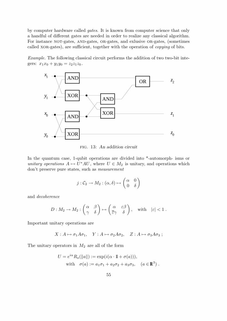
by computer hardware called gates. It is known from computer science that onlya handful of different gates are needed in order to realize any classical algorithm.For instance not-gates, and-gates, or-gates, and exlusive or-gates, (sometimescalled xor-gates), are sufficient, together with the operation of copying of bits.

Example. The following classical circuit performs the addition of two two-bit inte-gers: x1x0 + y1y0 = z2z1z0 .

XOR

AND

XOR

AND

AND

XOR

OR

y0

0x

y1

x1z2

z1

z0

fig. 13: An addition circuit

In the quantum case, 1-qubit operations are divided into *-automorph- isms orunitary operations A 7→ U∗AU , where U ∈ M2 is unitary, and operations whichdon’t preserve pure states, such as measurement

j : C2 →M2 : (α, δ) 7→(α 00 δ

)

and decoherence

D : M2 →M2 :

(α βγ δ

)7→(α εβεγ δ

), with |ε| < 1 .

Important unitary operations are

X : A 7→ σ1Aσ1, Y : A 7→ σ2Aσ2, Z : A 7→ σ3Aσ3 ;

The unitary operators in M2 are all of the form

U = eiαRa(‖a‖) := exp(i(α · 1l + σ(a))),

with σ(a) := a1σ1 + a2σ2 + a3σ3, (a ∈ IR3) .

55

The operation U∗ · U does not feel the phase α and acts on the Bloch sphere ofSection 2.2 as a rotation over an angle ‖a‖ around the axis IRa .

Exercises.1. Find values for α, ϑ and the unit vector u such that eiαRϑ(u) equals the

phase gate S :=

(1 00 i

)and the ‘π/8 gate’ or ‘T gate’ T :=

(1 00√i

)

respectively.

2. Find values for α, ϑ and u such that eiαRϑ(u) becomes the Hadamard matrix

H :=

(1 11 −1

).

Remark. We shall abuse the letters X,Y, Z,H, S, T by sometimes reading them asthe unitary matrices given above, sometimes as the associated operations. Thishas the slight advantage that diagrams in which these letters occur can be read interms of vector states in the Schrodinger picture, reading from left to right, or asoperations in the Heisenberg picture, reading from right to left. For their actionon density matrices in the Schrodinger picture stars have to be added.

The most important two-bit operation used in quantum computing is the con-trolled not gate which we met in Section 6.1. More generally we shall use the the‘controlled U ’ gate,

CU (M) :=

(1l 00 U∗

)M

(1l 00 U

), (M ∈M2 ⊗M2) .

symbolically denoted by the circuit

U

fig. 14: Controlled U gate

Lemma 7.1. Every controlled U gate on two qubits can be realised as a combina-tion of two controlled not gates and some single qubit operations.

Proof. Write U in terms of Euler angles:

U = eiαR3(β)R2(γ)R3(δ) .

56

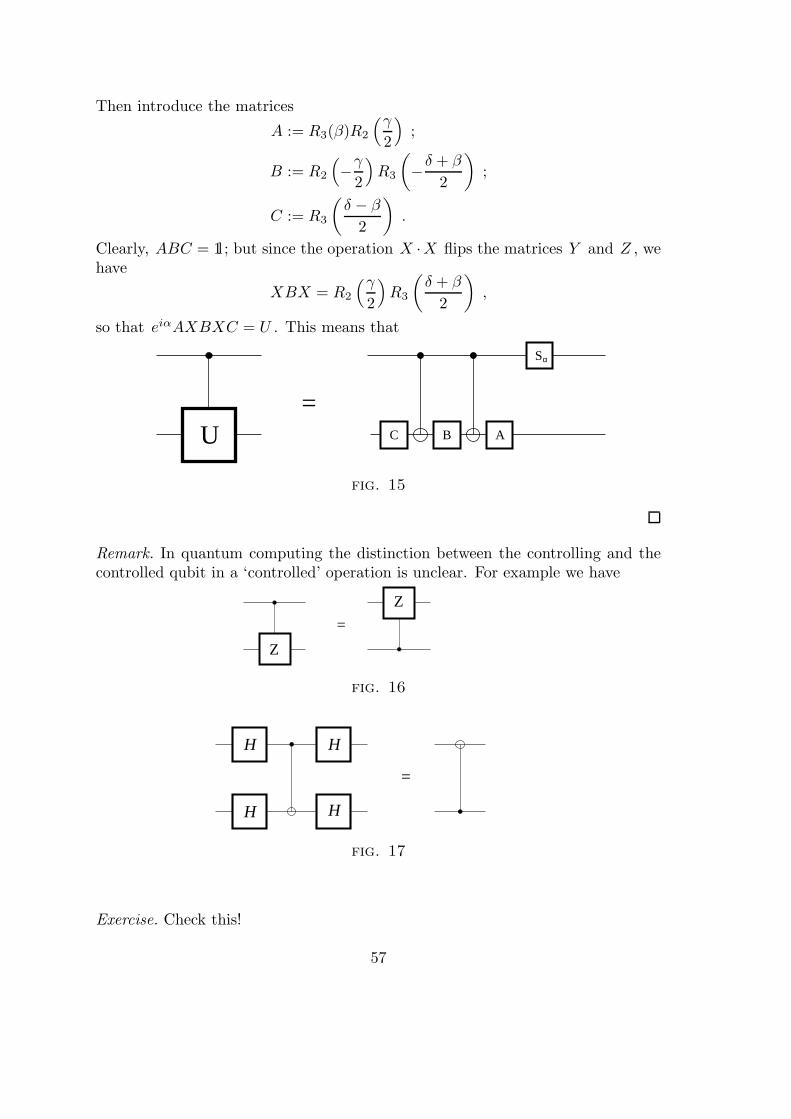
Then introduce the matrices

A := R3(β)R2

(γ2

);

B := R2

(−γ

2

)R3

(−δ + β

2

);

C := R3

(δ − β

2

).

Clearly, ABC = 1l; but since the operation X ·X flips the matrices Y and Z , wehave

XBX = R2

(γ2

)R3

(δ + β

2

),

so that eiαAXBXC = U . This means that

U=

Sα

C B A

fig. 15

Remark. In quantum computing the distinction between the controlling and thecontrolled qubit in a ‘controlled’ operation is unclear. For example we have

Z

=

Z

fig. 16

=

H

H

H

H

fig. 17

Exercise. Check this!

57

7.2 The quantum Fourier transform

Let N be a natural number, and consider the Hilbert space CN . Let FN denotethe discrete Fourier transform on this space, given by

(FNψ)(j) :=1√N

N−1∑

k=0

exp

(2πi

Njk

)ψ(k) . (11)

FN is a unitary transformation of CN and hence defines an operation (a *-automorphism) F ∗

N · FN on the algebra MN .

Now suppose that N is a power of 2: N = 2n . Then standard binary notationidentifies a natural number j < N with a bit sequence jn−1jn−2 · · · j1j0 such that

j =

n−1∑

l=0

jl 2l .

The space CN can be read as the n -fold tensor power of C2 , with the canonicalbasis

ej = ejn−1⊗ ejn−2

⊗ · · · ej1 ⊗ ej0 , (j = 0, . . .N − 1),

and FN becomes an n -qubit operation, which is known as the Quantum FourierTransform (QFT).

Proposition 7.2. The Quantum Fourier Transform maps the product vectorej = ejn−1

⊗ ejn−2⊗ · · · ej1 ⊗ ej0 to the product vector

1√2n

(e0 + exp(2πi(0.j0))e1

)⊗(e0 + exp(2πi(0.j1j0))e1

)

⊗ · · · ⊗(e0 + exp(2πi(0.jn−1 · · · j1j0))e1

),

(12)

where 0, jq · · · j1j0 denotes the binary fraction∑qm=0 jm2m−q−1 .

Proof. We calculate

FNej =1√N

N−1∑

k=0

exp

(2πi

Nk · j

)ek

=1√2n

1∑

k0=0

· · ·1∑

kn−1=0

n−1⊗

l=0

exp

(2πi

2nkl2

l · j)ekl

=

n−1⊗

l=0

(e0 + exp

(2πi

j

2n−l

)e1

)/√

2

=

n−1⊗

l=0

(e0 + exp

(2πi

jn−l−1 · · · j1j02n−l

)e1

)/√

2

The tensor product should be written from right to left as the running indexincreases.

58

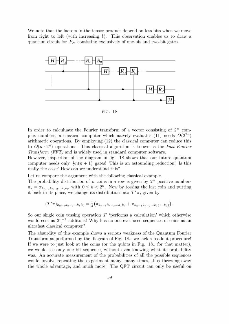
We note that the factors in the tensor product depend on less bits when we movefrom right to left (with increasing l ). This observation enables us to draw aquantum circuit for FN consisting exclusively of one-bit and two-bit gates.

Rn-1

RH

R Rnn-1

n-2

RH

RH

H

2

2

fig. 18

In order to calculuate the Fourier transform of a vector consisting of 2n com-plex numbers, a classical computer which naively evaluates (11) needs O(22n)arithmetic operations. By employing (12) the classical computer can reduce thisto O(n · 2n) operations. This classical algorithm is known as the Fast FourierTransform (FFT) and is widely used in standard computer software.However, inspection of the diagram in fig. 18 shows that our future quantumcomputer needs only 1

2n(n + 1) gates! This is an astounding reduction! Is thisreally the case? How can we understand this?

Let us compare the argument with the following classical example.The probability distribution of n coins in a row is given by 2n positive numbersπk = πkn−1kn−2...k1k0 with 0 ≤ k < 2n . Now by tossing the last coin and puttingit back in its place, we change its distribution into T ∗π , given by

(T ∗π)kn−1kn−2...k1k0 = 12

(πkn−1kn−2...k1k0 + πkn−1kn−2...k1(1−k0)

).

So our single coin tossing operation T ‘performs a calculation’ which otherwisewould cost us 2n−1 additons! Why has no one ever used sequences of coins as anultrafast classical computer?

The absurdity of this example shows a serious weakness of the Quantum FourierTransform as performed by the diagram of Fig. 18.: we lack a readout procedure!If we were to just look at the coins (or the qubits in Fig. 18., for that matter),we would see only one bit sequence, without even knowing what its probabilitywas. An accurate measurement of the probabilities of all the possible sequenceswould involve repeating the experiment many, many times, thus throwing awaythe whole advantage, and much more. The QFT circuit can only be useful on

59

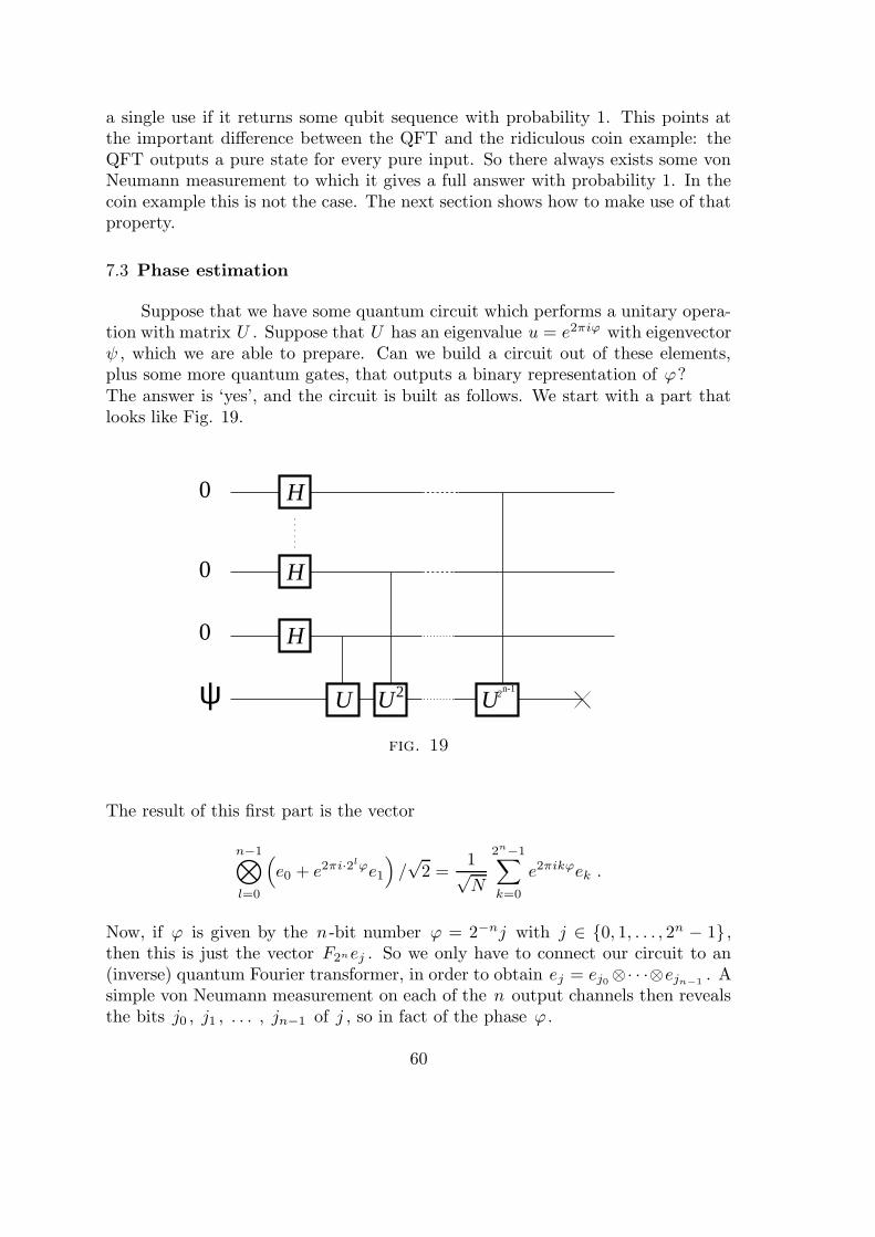
a single use if it returns some qubit sequence with probability 1. This points atthe important difference between the QFT and the ridiculous coin example: theQFT outputs a pure state for every pure input. So there always exists some vonNeumann measurement to which it gives a full answer with probability 1. In thecoin example this is not the case. The next section shows how to make use of thatproperty.

7.3 Phase estimation

Suppose that we have some quantum circuit which performs a unitary opera-tion with matrix U . Suppose that U has an eigenvalue u = e2πiϕ with eigenvectorψ , which we are able to prepare. Can we build a circuit out of these elements,plus some more quantum gates, that outputs a binary representation of ϕ?The answer is ‘yes’, and the circuit is built as follows. We start with a part thatlooks like Fig. 19.

0

ψ

0

0

U2 2n-1

UU

H

H

H

fig. 19

The result of this first part is the vector

n−1⊗

l=0

(e0 + e2πi·2

lϕe1

)/√

2 =1√N

2n−1∑

k=0

e2πikϕek .

Now, if ϕ is given by the n -bit number ϕ = 2−nj with j ∈ 0, 1, . . . , 2n − 1 ,then this is just the vector F2nej . So we only have to connect our circuit to an(inverse) quantum Fourier transformer, in order to obtain ej = ej0⊗· · ·⊗ejn−1

. Asimple von Neumann measurement on each of the n output channels then revealsthe bits j0 , j1 , . . . , jn−1 of j , so in fact of the phase ϕ .

60

If ϕ is not a multiple of 2−n , then the algorithm can still be used, yielding naccurate bits of ϕ with probability 1 − ε , provided that we use a number t ofqubits given by

t = n+

⌈log

(2 +

1

2ε

)⌉.

(See [NiC] Section 5.2.1.)

7.4 Finding the order

Let N be a (large) integer number between 2L−1 and 2L , and let x be asmaller integer, coprime with N . Then the map

ux : 0, . . . , N − 1 → 0, . . . , N − 1 : y 7→ xy (modN)

is injective and hence invertible. It follows that, if we start with 1, and apply thismap repeatedly, we must return to 1 after some number r of iterations. This cyclelength is called the order of x modulo N .Let Ux denote the unitary operator CN → CN associated to the permutation ux ,and let Hx ⊂ CN be the r -dimensional subspace spanned by the Ukx e1 . Then thespectrum of the restriction of Ux to Hx consists of the r -th roots of unity, eachhaving multiplicity 1. This establishes a connection between the order r of x andthe eigenvalues of Ux , which permits us to find r using the quantum algorithmof phase estimation treated in §7.3. This program has several aspects to it, whichwe shall treat in succession.

A. Building controlled Ux -gates out of our knowledge of x and N ;

B. finding a suitable input vector ψ for the phase algorithm;

C. distilling r from the measured phase.

A. Modular exponentiation. We wish to implement by quantum gates themap

ez ⊗ ey 7→ ez ⊗ exzy ,

where we count modulo N in the indices. This can be done using unitary ex-tensions of classical gates, put together according to do the binary multiplicationy 7→ xy , followed by Euclid’s algorithm for the remainder modulo N .

B. Choosing an input vector. Ideally we would like to have an eigenvector ψof Ux to use as an input, but this requires knowledge of the order r itself, whichis out of the question. As our second best we can take e1 as an input, since thisvector is proportional to the sum of the eigenvectors of Ux in Hx :

e1 =1√r

r−1∑

s=0

ψs ,

61

where ψs , for s ∈ 0, . . . , r − 1 given by

ψs :=1√r

r−1∑

k=0

e2πi

rskexk ,

is an eigenvector:

Uxψs = e2πi

rsψs .

Since the calculations under A are done in a unitary way, preserving linear com-binations, the result of the phase estimation is a binary expression for

ϕ =s

r,

where s is chosen at random from the set 0, 1, . . . , r − 1 .

C. Continued fraction expansion. The final part is a purely classical calcu-lation. Suppose we obtain a 2L -bit approximation ϕ′ to ϕ = s/r , i.e., ϕ′ is amultiple of 2−L satisfying |ϕ − ϕ′| < 2−L . Then ϕ = s/r occurs as a term inthe continued fraction expansion of ϕ′ . (See [NiC].) This gives us explicit integervalues for s′ and r′ satisfying s′/r′ = s/r . If we are lucky, which happens areasonable fraction of the time, then s and r are coprime, so that r′ is the actualorder of x . This is easily tested by calcululating xr in the classical way.

7.5 Factorization

The reduction of factoring to order-finding proceeds in two basic steps. Thefirst step is to show that we can compute a factor of N if we can find a non-trivialsolution x 6= ±1(modN) to the equation x2 = 1(modN). The second step is toshow that a randomly chosen y coprime to N is quite likely to have an order rwhich is even, and such that yr/2 6= ±1 (modN), thus yielding x = yr/2 satisfyingthe above.These two steps are embodies in the following two theorems. We shall only provethe easy one, referring the reading to the literature for the other.

Theorem 7.3. Suppose N is an L bit composite number, and x ∈ 2, . . . , N−2is a solution to the equation x2 = 1(modN) . Then at least one of gcd(x− 1, N)and gcd(x+ 1, N) is a non-trivial factor of N , and can be computed using O(L3)operations.

Proof. Since x2 = 1(modN), it must be that N divides x2 − 1 = (x+ 1)(x− 1),and thus N must have a common factor with x + 1 or with x − 1. By theassumption on x this can not be N itself. Using Euclid’s algorithm we maycompute gcd(x − 1, N and gcd(x + 1, N) and thus obtain a non-trivial factor ofN , using O(L3) operations.

62

Theorem 7.4. Suppose N = pα1

1 pα2

2 · · · pαmm is the prime factorization of an odd

composite positive integer. Let x be an integer chosen at random, subject to therequirements that 1 ≤ x ≤ N − 1 and x is coprime to N . Let r be the order ofx modulo N . Then

IP[r is even and xr/2 6= −1 (modN)] ≥ 1− 1

2m.

Proof. See [NiC].

8. Public key cryptography: the RSA cryptosystem

In 1978 R.L. Rivest, A. Shamir and L. Adleman proposed a public key cryp-tosystem that has become known as the RSA system. Although it lies outsidethe strict scope of Quantum Computing, being a purely classical algorithm, it isworthwhile treating it here, since its potential vulnerability to Shor’s quantumalgorithm is such a powerful motivation for the field of Quantum Computing as awhole.

Public key cryptography is the art of devising codes that can be used bythe public to encipher messages, but enable only a few authorised persons todecipher them. It is an intriguing fact that such codes are possible at all. TheRSA cryptosystem relies on the essential one-way character of multiplication of(large prime) numbers: with the help of a computer it is easy to multiply numbersof — say — 200 digits each, but it is practically impossible to disentangle thesefactors from their product if you don’t know them, even if these factors are primenumbers, and therefore determined in principle by the product.

The motor of the RSA system is an elementary result in number theory:Fermat’s ‘little’ theorem.

Theorem 8.1 (Fermat) Let p be a prime number, and x any positive integer,not divisible by p . Then

xp−1 ≡ 1 (mod p) .

Proof. As p is prime, the map

0, . . . , p− 1 → 0, . . . , p− 1 : y 7→ xy (mod p)

is a permutation. Apart from the trivial cycle 0 all cycles of this permutationhave the same length, which is the order r of 1. Indeed if xky ≡ y , then (xk−1)y ≡0, and since p is prime we must have y ≡ 0 or xk ≡ 1. Thus r must be a divisorof p− 1, say p− 1 = ar , and

xp−1 = xar = (xr)a = 1a = 1 .

63

Corollary 8.2. Let p and q be prime numbers, and x any positive integer, notdivisible by p or by q . Then

x(p−1)(q−1) ≡ 1 (mod pq) .

Proof. By Fermat’s Theorem, x(p−1)(q−1) ≡ 1 both modulo p and modulo q ,hence modulo pq .

A second result from elementary number theory is also indispensible for an under-standing of the RSA system:

Theorem 8.3 (Euclid’s algorithm) Given two positive integers a and b it ispossible to effectively calculate gcd(a, b) and integers u and v such that

gcd(a, b) = ua+ vb .

Proof. The algorithm goes as follows. Suppose that a > b . Put

a0 := a ; a1 := b ;

u0; = 1 ; u1 := 0 ;

v0; = 0 ; v1 := 1 .

Then repeat, starting from k := 1 until n , where n is the first value of k forwhich ak+1 = 0:

mk := [ak−1/ak] ;

ak+1 := ak−1 −mkak ;

uk+1 := uk−1 −mkuk ;

vk+1 := vk−1 −mkvk .

Then at each stage we have

gcd(ak−1, ak) = gcd(a, b) and ak = uka+ vkb .

In particular for k = n . But then an−1 = mnan , so that an = gcd(a, b) =una+ vnb .The algorithm is bound to halt since a0 > a1 > a2 > . . .; it is exponentially fastsince ak+2 ≤ 1

2ak for all k .

8.1 The RSA system

The central authority (let us call her Alice) chooses two large primes p andq , say about 200 digits long. (This is possible! There are reliable and effectivestochastic primality tests for large integers.) She keeps these numbers secret,but publishes their product N := pq . Then she calculates the secret number

64

S := (p − 1)(q − 1) and chooses an integer 1 < e < S such that gcd(e, S) = 1.(There are plenty of such numbers, hence she can just choose a number at randomand then test coprimality using Euclid’s algorithm). This number e , the encodingcipher is also published.

If somebody from the public (let us call him Bob) wishes to send a secretmessage to Alice, he first encodes his message into a number m between 0 andN − 1, and then calculates the code

c := me (modN) ,

which he sends to Alice over a public channel. The point now is that, although thecalculation of c from m can be done quite easily, by repeated squaring of m , andmultiplying only those powers that correspond to a 1 in the binary expansion ofe , it is practically impossible to find m back if c , e and N are known. No muchbetter methods are known to do this, than to calculate the e -th power modulo Nof all possible messages.

However, for Alice the situation is different. Since she knows S , and sincegcd(S, e) = 1, she can use Euclid’s extended algorithm to calculate numbers dand b such that

de− bS = 1 , i.e. de ≡ 1 (modS) .

She then uses the decoding cipher d to calculate m from c :

cd = med = m1+bS = m ·mb(p−1)(q−1) ≡ m (modN) ,

where in the last step Corollary 8.2 is used.

Exercise. What happens if by accident the code m is divisible by p or by q?

9. The quantum Monty Hall problem *

The well-known (classical) Monty Hall problem or three-door problem is setin the context of a television game show. It can be seen as a two person game, inwhich a player P tries to win a prize, but a show master (or Quiz master) Q triesto make it difficult for her. This game can be ‘quantized’, i.e., its key elementscan be formulated in a quantum mechanical context, allowing new strategies andnew solutions.

* This chapter is based on: Mauro D’Ariano, Richard Gill, Michael Keyl, Rein-hard Werner, Burkhard Kummerer, Hans Maassen: The quantum Monty Hallproblem, Quantum Information and Computing, 2 (2002) 355-366.

65

9.1 The classical Monty Hall problem

In the last round of a television show, the candidates are given a chance tocollect their prize (or lose it) in the following game:

1. Before the show the prize is hidden behind one of three closed doors. Theshow master knows where the prize is but, of course, the candidate does not.

2. The candidate is asked to choose one of the three doors, which is, however,not opened at this stage.

3. The show master opens another door, and shows that there is no prize behindit. (He can do this, because he knows where the prize is).

4. The candidate can now open one of the remaining doors to either collect herprize or lose.

The question is: should the candidate stick to her original choice or “change hermind” and pick the other remaining door? As a quick test usually shows, mostpeople will stick to their first choice. After all, before the show master opened adoor the two doors were equivalent, and they were not touched (nor was the prizemoved). So they should still be equivalent. This argument seems so obvious thattrained mathematicians and physicists fall for it almost as easily as anybody else.However, the correct solution by which the candidates can, in fact, double theirchance of winning, is to always choose the other door. The quickest way to convincepeople of this is to compare the game with another one, in which the show masteroffers the choice of either staying with your choice or opening both other doors.Anybody would prefer that, especially if the show master courteously offers toopen one of the doors for you. But this is precisely what happens in the originalgame when you always change to the other door.

9.2 The quantum Monty Hall problem

We will “quantize” only the key parts of the problem. That is, the prize andthe players, as well as their publicly announced choices, will remain classical. Thequantum version can even be played in a game show on classical TV.

The main quantum variable will be the position of the prize. It lies in a3-dimensional complex Hilbert space H , called the game space. We assume thatan orthonormal basis is fixed for this space so that vectors can be identified bytheir components, but apart from this the basis has no significance for the game.A second important variable in the game is what we will call the show master’snotepad. This might be classical information describing how the game space wasprepared, or it might be a quantum system, entangled with the prize. In thelatter case, the show master is able to do a quantum measurement on his notepad,providing him with classical information about the prize, without moving theprize, in the sense that the player’s information about the prize is not changedby the mere fact that the show master “consults his notepad”. A measurement

66

on an auxiliary quantum system, even if entangled with a system of interest, doesnot alter the reduced state of the system of interest. After the show master hasconsulted his notepad, we are in the same situation as if the notepad had been aclassical system all along. As in the classical game, the situation for the playermight change when the show master, by opening a door, reveals to some extentwhat he saw in his notepad. Opening a door corresponds to a measurement alonga one dimensional projection on H .

The game proceeds in the following stages, closely analogous to the classicalgame:

1. Before the show the game space system is prepared quantum mechanically.Some information about this preparation is given to the show master Q. Thiscan be in the form of another system, called the notepad, which is in a statecorrelated with the game space.

2. The candidate chooses some one dimensional projection p on H .

3. The show master opens a door, i.e., he chooses a one dimensional projectionq , and makes a von Neumann measurement with projections q and (1l−q). Inorder to do this, he is allowed first to consult his notebook. If it is a quantumsystem, this means that he carries out a measurement on the notebook. Thejoint state of prize and notebook then change, but the traced out or reducedstate of the prize does not change, as far as the player is concerned. Tworules constrain the show master’s choice of q : he must choose “another door”in the sense that q ⊥ p ; and he must be certain not to reveal the prize. Thepurpose of his notepad is to enable him to do this. After these steps, thegame space is effectively collapsed to the two-dimensional space (1l− q)H .

4. The player P can now choose a one dimensional projection p′ on (1l− q)H ,and the corresponding measurement on the game space is carried out. If itgives “yes” she collects the prize.

As in the classical case, the question is: how should the player choose the projectionp′ in order to maximize her chance of winning?

From the classical case it seems likely that choosing p′ = p is a bad idea. Solet us say that the classical strategy in this game consists of always switching tothe orthogonal complement of the previous choice, i.e., to take p′ = 1l−q−p . Notethat this is always a projection because, by rule 3, p and q are orthogonal onedimensional projections. We will analyze this strategy in Section ?, which turnsout to be possible without any specification of how the show master can guaranteenot to stumble on the prize in step 3.There are two main ways the show master can satisfy the rules. The first is that hechooses randomly the components of a vector in H , and prepares the game spacein the corresponding pure state. He can then just take a note of his choice on aclassical pad, so that in stage 3 he can compute a vector orthogonal to both thedirection of the preparation and the direction chosen by the player. Q’s strategiesin this case are discussed in Section 9.5. The second and more interesting way is

67

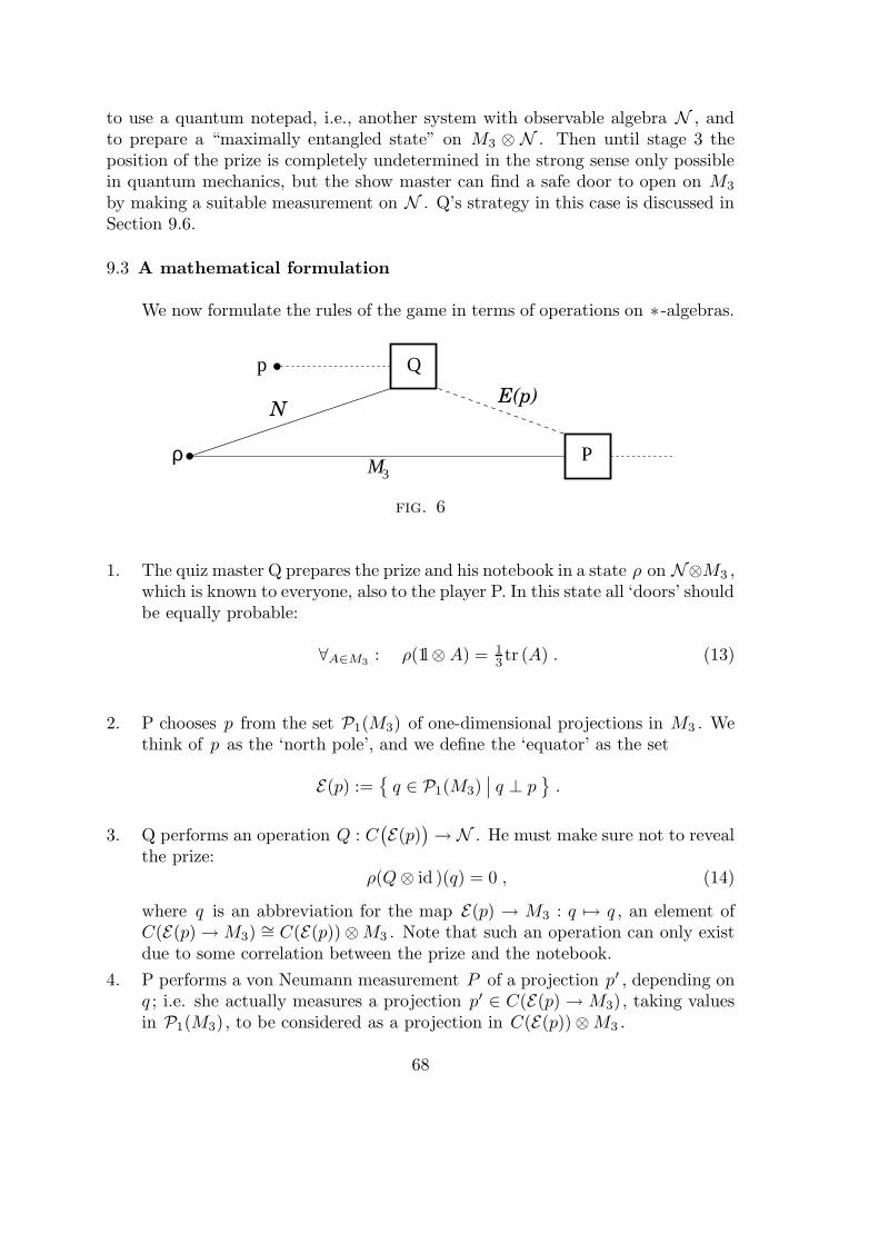
to use a quantum notepad, i.e., another system with observable algebra N , andto prepare a “maximally entangled state” on M3 ⊗ N . Then until stage 3 theposition of the prize is completely undetermined in the strong sense only possiblein quantum mechanics, but the show master can find a safe door to open on M3

by making a suitable measurement on N . Q’s strategy in this case is discussed inSection 9.6.

9.3 A mathematical formulation

We now formulate the rules of the game in terms of operations on ∗ -algebras.

NE(p)

3M

p

P

Q

ρ

fig. 6

1. The quiz master Q prepares the prize and his notebook in a state ρ on N⊗M3 ,which is known to everyone, also to the player P. In this state all ‘doors’ shouldbe equally probable:

∀A∈M3: ρ(1l⊗ A) = 1

3tr (A) . (13)

2. P chooses p from the set P1(M3) of one-dimensional projections in M3 . Wethink of p as the ‘north pole’, and we define the ‘equator’ as the set

E(p) :=q ∈ P1(M3)

∣∣ q ⊥ p.

3. Q performs an operation Q : C(E(p)

)→ N . He must make sure not to reveal

the prize:ρ(Q⊗ id )(q) = 0 , (14)

where q is an abbreviation for the map E(p) → M3 : q 7→ q , an element ofC(E(p)→M3) ∼= C(E(p))⊗M3 . Note that such an operation can only existdue to some correlation between the prize and the notebook.

4. P performs a von Neumann measurement P of a projection p′ , depending onq ; i.e. she actually measures a projection p′ ∈ C(E(p)→ M3), taking valuesin P1(M3), to be considered as a projection in C(E(p))⊗M3 .

68

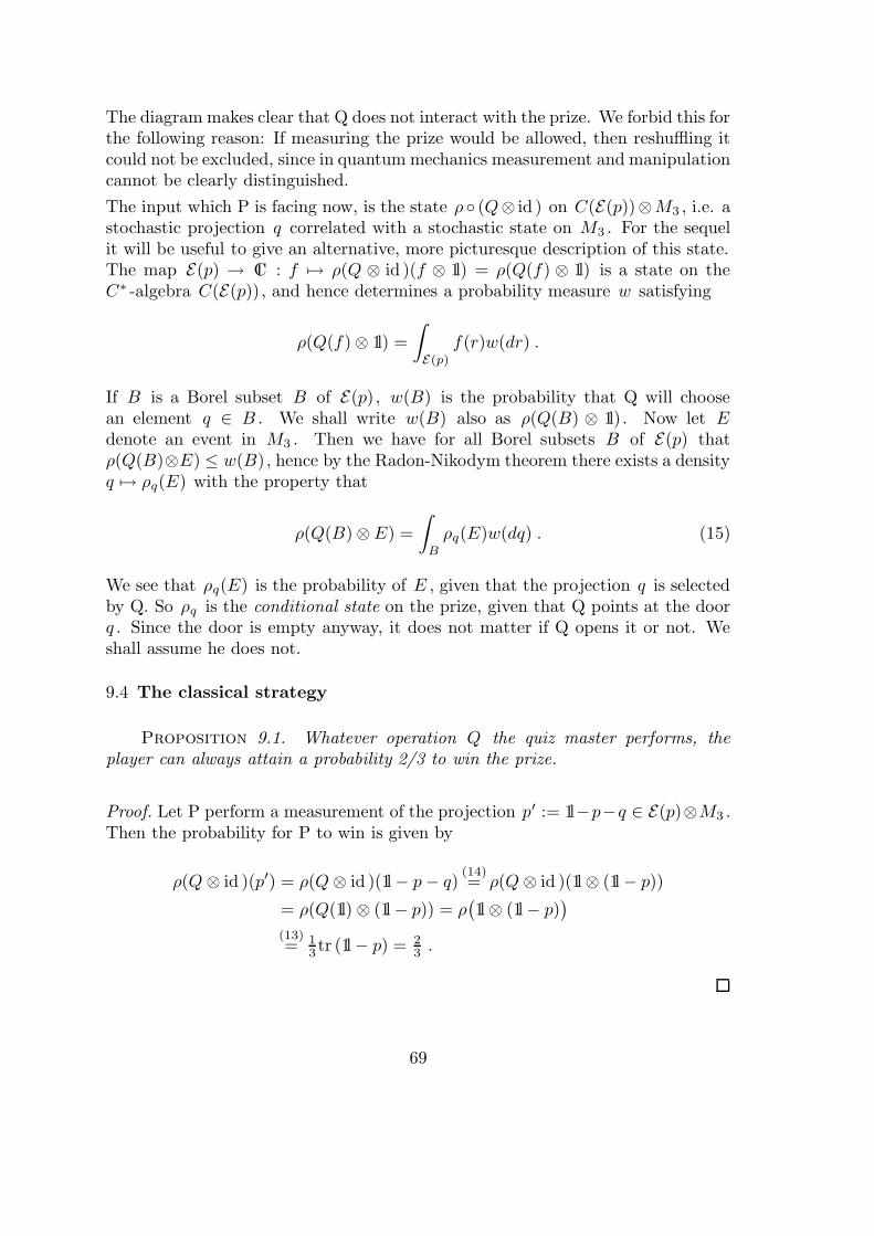
The diagram makes clear that Q does not interact with the prize. We forbid this forthe following reason: If measuring the prize would be allowed, then reshuffling itcould not be excluded, since in quantum mechanics measurement and manipulationcannot be clearly distinguished.

The input which P is facing now, is the state ρ (Q⊗ id ) on C(E(p))⊗M3 , i.e. astochastic projection q correlated with a stochastic state on M3 . For the sequelit will be useful to give an alternative, more picturesque description of this state.The map E(p) → C : f 7→ ρ(Q ⊗ id )(f ⊗ 1l) = ρ(Q(f) ⊗ 1l) is a state on theC∗ -algebra C(E(p)), and hence determines a probability measure w satisfying

ρ(Q(f)⊗ 1l) =

∫

E(p)

f(r)w(dr) .

If B is a Borel subset B of E(p), w(B) is the probability that Q will choosean element q ∈ B . We shall write w(B) also as ρ(Q(B) ⊗ 1l). Now let Edenote an event in M3 . Then we have for all Borel subsets B of E(p) thatρ(Q(B)⊗E) ≤ w(B), hence by the Radon-Nikodym theorem there exists a densityq 7→ ρq(E) with the property that

ρ(Q(B)⊗ E) =

∫

B

ρq(E)w(dq) . (15)

We see that ρq(E) is the probability of E , given that the projection q is selectedby Q. So ρq is the conditional state on the prize, given that Q points at the doorq . Since the door is empty anyway, it does not matter if Q opens it or not. Weshall assume he does not.

9.4 The classical strategy

Proposition 9.1. Whatever operation Q the quiz master performs, theplayer can always attain a probability 2/3 to win the prize.

Proof. Let P perform a measurement of the projection p′ := 1l−p−q ∈ E(p)⊗M3 .Then the probability for P to win is given by

ρ(Q⊗ id )(p′) = ρ(Q⊗ id )(1l− p− q) (14)= ρ(Q⊗ id )(1l⊗ (1l− p))

= ρ(Q(1l)⊗ (1l− p)) = ρ(1l⊗ (1l− p)

)

(13)= 1

3 tr (1l− p) = 23 .

69

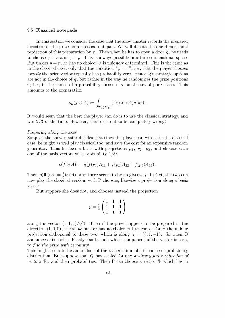
9.5 Classical notepads

In this section we consider the case that the show master records the prepareddirection of the prize on a classical notepad. We will denote the one dimensionalprojection of this preparation by r . Then when he has to open a door q , he needsto choose q ⊥ r and q ⊥ p . This is always possible in a three dimensional space.But unless p = r , he has no choice: q is uniquely determined. This is the same asin the classical case, only that the condition “p = r”, i.e., that the player choosesexactly the prize vector typically has probability zero. Hence Q’s strategic optionsare not in the choice of q , but rather in the way he randomizes the prize positionsr , i.e., in the choice of a probability measure µ on the set of pure states. Thisamounts to the preparation

ρµ(f ⊗ A) :=

∫

P1(M3)

f(r)tr (rA)µ(dr) .

It would seem that the best the player can do is to use the classical strategy, andwin 2/3 of the time. However, this turns out to be completely wrong!

Preparing along the axesSuppose the show master decides that since the player can win as in the classicalcase, he might as well play classical too, and save the cost for an expensive randomgenerator. Thus he fixes a basis with projections p1 , p2 , p3 , and chooses eachone of the basis vectors with probability 1/3:

ρ(f ⊗ A) := 13(f(p1)A11 + f(p2)A22 + f(p3)A33) .

Then ρ(1l⊗A) = 13tr (A), and there seems to be no giveaway. In fact, the two can

now play the classical version, with P choosing likewise a projection along a basisvector.

But suppose she does not, and chooses instead the projection

p = 13

1 1 11 1 11 1 1

along the vector (1, 1, 1)/√

3. Then if the prize happens to be prepared in thedirection (1, 0, 0), the show master has no choice but to choose for q the uniqueprojection orthogonal to these two, which is along χ = (0, 1,−1). So when Qannounces his choice, P only has to look which component of the vector is zero,to find the prize with certainty!This might seem to be an artifact of the rather minimalistic choice of probabilitydistribution. But suppose that Q has settled for any arbitrary finite collection ofvectors Ψα and their probabilities. Then P can choose a vector Φ which lies in

70

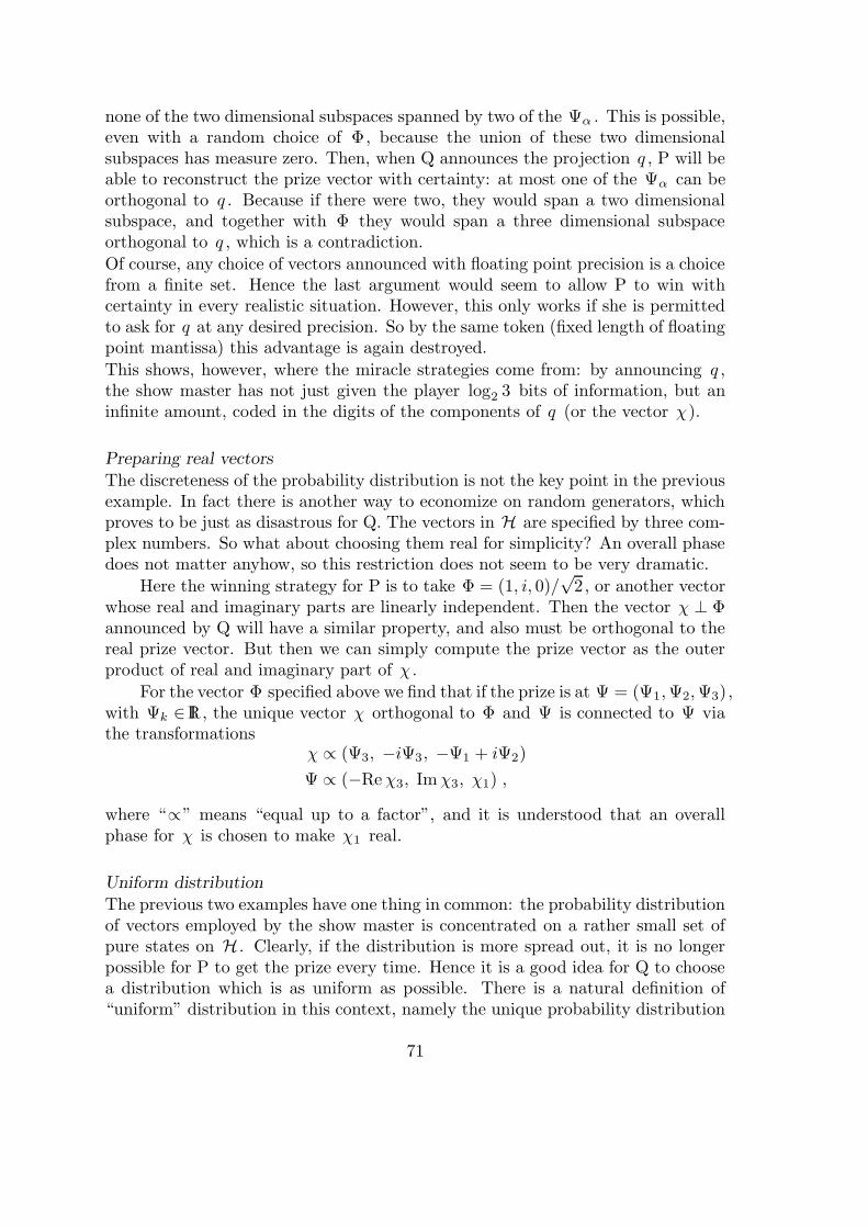
none of the two dimensional subspaces spanned by two of the Ψα . This is possible,even with a random choice of Φ, because the union of these two dimensionalsubspaces has measure zero. Then, when Q announces the projection q , P will beable to reconstruct the prize vector with certainty: at most one of the Ψα can beorthogonal to q . Because if there were two, they would span a two dimensionalsubspace, and together with Φ they would span a three dimensional subspaceorthogonal to q , which is a contradiction.

Of course, any choice of vectors announced with floating point precision is a choicefrom a finite set. Hence the last argument would seem to allow P to win withcertainty in every realistic situation. However, this only works if she is permittedto ask for q at any desired precision. So by the same token (fixed length of floatingpoint mantissa) this advantage is again destroyed.

This shows, however, where the miracle strategies come from: by announcing q ,the show master has not just given the player log2 3 bits of information, but aninfinite amount, coded in the digits of the components of q (or the vector χ).

Preparing real vectors

The discreteness of the probability distribution is not the key point in the previousexample. In fact there is another way to economize on random generators, whichproves to be just as disastrous for Q. The vectors in H are specified by three com-plex numbers. So what about choosing them real for simplicity? An overall phasedoes not matter anyhow, so this restriction does not seem to be very dramatic.

Here the winning strategy for P is to take Φ = (1, i, 0)/√

2, or another vectorwhose real and imaginary parts are linearly independent. Then the vector χ ⊥ Φannounced by Q will have a similar property, and also must be orthogonal to thereal prize vector. But then we can simply compute the prize vector as the outerproduct of real and imaginary part of χ .

For the vector Φ specified above we find that if the prize is at Ψ = (Ψ1,Ψ2,Ψ3),with Ψk ∈ IR, the unique vector χ orthogonal to Φ and Ψ is connected to Ψ viathe transformations

χ ∝ (Ψ3, −iΨ3, −Ψ1 + iΨ2)

Ψ ∝ (−Reχ3, Imχ3, χ1) ,

where “∝” means “equal up to a factor”, and it is understood that an overallphase for χ is chosen to make χ1 real.

Uniform distribution

The previous two examples have one thing in common: the probability distributionof vectors employed by the show master is concentrated on a rather small set ofpure states on H . Clearly, if the distribution is more spread out, it is no longerpossible for P to get the prize every time. Hence it is a good idea for Q to choosea distribution which is as uniform as possible. There is a natural definition of“uniform” distribution in this context, namely the unique probability distribution

71

on the unit vectors, which is invariant under arbitrary unitary transformations. Isthis a good strategy for Q?

Proposition 9.2. If Q prepares the prize in a pure state chosen uniformlyat random, keeping a classical note of this pure state, then P cannot raise hisprobability of winning above 2/3.

In other words, the pair of strategies: “uniform distribution for Q and classicalstrategy for P” is an equilibrium point of the game. We do not know yet, whetherthis equilibrium is unique, in other words: If Q does not play precisely by theuniform distribution: can P always improve on the classical strategy? We supposethat the answer to this question is yes, to find a proof of this conjecture has turnedout, however, to be a hard problem.

Remark. Although this is clearly an optimal situation for the show master, it mustbe noted that he needs in principle an infinitely large notebook, since he has torecord in it the pure state in which the prize was prepared with infinite accuracy.Any finite notebook falls into the trap of Section 9.3.

Proof. Let µ0 be the rotation invariant probability measure on P1(M3). The ρµ0

is rotation iinvariant in the sense that for all f ∈ C(P1(M3)), A,U ∈ M3 , Uunitary:

ρ(fU , U∗AU) = ρ(f, U) ,

where fU (r) := f(U∗rU). But then, for all p ∈ P1(M3), all U commuting withp and g ∈ C(E(p)):

ρµ0(Q⊗ id )(gU ⊗ U∗AU) = ρµ0

(Q⊗ id )(g ⊗ A) .

Formulating this in terms of the conditional state ρq we obtain that∫

E(p)

g(U∗qU)tr (ρqU∗AU)w(dq) =

∫

E(p)

g(q)tr (ρqA)w(dq) .

It follows that for all q ∈ E(p):UρqU

∗ = ρUqU∗ . (16)

In particular, if Uq = qU we have Uρq = ρqU . So ρq commutes with every Ucommuting with p and q :

ρq ∈ p, q′′, hence ρq = αqp+ βqq + γq(1l− p− q) .Now, βq = tr (qρq) = 0 by (14) and (15); αq does not depend on q because of(16); αq + γq = tr (ρq) = 1 and

αq = α =

∫tr (pρq)w(dq) = ρµ0

(Q⊗ id )(1l⊗ p) = ρµ0(1l⊗ p) = 1

3tr (p) = 13 .

We find that

ρq =1

3p+

2

3(1l− p− q) .

Hence the classical strategy for P is clearly optimal.

72

9.6 A quantum notebook

Finally consider the situation where the quiz master posesses a quantum ‘note-book’, which is an exact copy of the prize.

Proposition 9.3. If Q prepares the prize and the notebook in the maximallyentangled state ω of Section 4.4, then again P cannot raise his probability ofwinning above 2/3.

Proof. Let p = p1 , p2 and p3 be orthogonal projections in M3 . Q is the followingaction: Measure p2 ; if yes then point at p3 , else at p2 . So

Qg := g(p2)(p1 + p2) + g(p3)p2 .

Let p′ be any strategy for P. Then

ω(Q⊗ id )(p′) = ω(p′(p2)⊗ (p1 + p3) + p′(p3)⊗ p2)

= 13tr(p′(p2)

T (p1 + p3))

+ 13tr(p′(p3)

T p2

)

≤ 13 tr p′(p2) + 1

3 tr p′(p3) = 23 .

We note that the show master can only avoid needing an infinite amount of infor-mation by using a quantum notebook. So here is another situation where quantuminformation is superior to classical information.We admit that this is partly due to the very harsh rule (14) that Q is not allowedto risk revealing the prize, which forces him to betray its location. An interestingversion of the game would be to put no such restriction on Q’s behaviour, but togive the prize away whenever it appears behind the door opened by Q. Classically,Q has nothing to gain in taking this risk, but in the quantum situation he mayprofit from this possibility!

10. Quantum Markov chains

The notion of a Markov chain has been generalised by Kummerer outside thecontext of probability, to something that is meaningful in an arbitrary category.The aim of this generalisation was to motivate the definition of a ‘quantum Markovchain’ given by Accardi, Frigerio and Lewis in the early 1980’s. As a by-productthe older ‘unitary dilations’ of Sz.-Nagy and Foias were incorporated into the samescheme.The main idea is, that a Markov chain is a dilation (a ‘blowing up’) of a semigroupof arbitrary operations to a group of invertible operations, in the same way as adissipative evolution in physics can always be extended to a world that evolvesreversibly.

73

10.1 Classical Markov chains on finite state spaces

Let Ω be a finite set, and let T be a transition probability matrix on Ω withinvariant probability distribution ϕ :

T = (tij)i,j∈Ω, tij ∈ [0, 1] ;

∀i∈Ω :∑

j∈Ω

tij = 1, ∀j∈Ω :∑

i∈Ω

ϕitij = ϕj .

(See Section 4.1 and 4.2 for this notation.)It is a well-known result in probability theory that such a structure (Ω, ϕ, T )determines a stationary Markov chain, i.e. a sequence of random variables

X0, X1, X2, . . .

on a probability space (Ω,Σ, IP) such that for all i, j ∈ Ω and n ∈ IN,

IP[X0 = i] = ϕi and

IP[Xn+1 = j|X0 = i0, . . . , Xn = in = i] = IP[Xn+1 = j|Xn = i] = tij .

Now, as ϕ is stationary, the sequence of random variables can be extended to atwo-sided infinite sequence

. . . , X−2, X−1, X0, x1, X2, . . .

and we may assume that Σ is generated by these random variables. Because ofthis minimality assumption, and since the process (Xn)n∈Z is stationary, there

exists a map τ : Ω→ Ω connecting the random variables:

Xn+1 = Xn τ .

A concrete choice for Ω is ΩZ , the space of all infinite paths through Ω, and inthis case τ is simply the left shift:

τ(ω)n = ωn+1 .

In the above familiar situation we now distinguish two ‘layers’, which become moreclear if we formulate matters in terms of algebras, as we have done all the time inthese notes.Let A := C(Ω). Then the triple (A, ϕ, T ) forms the ‘upper layer’.

In the ‘lower layer’, let A denote the algebra L∞(Ω,Σ, IP), generated by functionsof the form (Xn)n∈Z because of our minimality assumption. Let us consider the

left shift as an operator on the functions on Ω:

T : A → A :(T g)(ω) := g

(τ(ω)

).

74

We have now arranged our notation in such a way that (A, ϕ, T ) and (A, ϕ := IP, T )are very similar structures; we call them both (stochastic) dynamical systems. An

important difference is, however, that T is invertible, and (Tn)n∈Z is a group of

automorphisms of (A, ϕ), whereas (Tn)n∈IN is an arbitrary semigroup of opera-tions on (A, ϕ).

Moreover, (A, ϕ, T ) can be embedded into (A, ϕ, T ) by the map

j : A → A : f 7→ f X0 .

(In fact there is such an embedding jn : f 7→ f Xn for all n ∈ ZZ , which can be

written as Tn j .)Associated to j there is a conditional expectation (see Section 4.2)

E : A → A : g 7→ IE(g|X0) ,

which is the left-inverse of j : E j = id A .Now, the dynamical systems (A, ϕ, T ) and (A, ϕ, T ) are related by

E(f(Xn)

∣∣X0

): i0 7→

∑

i0∈Ω

∑

i1∈Ω

· · ·∑

in∈Ω

ti0i1 · · · tin−1inf(in) = (Tnf) (i0) ,

for all n ∈ IN. In other words, since f(Xn) = f X0 τn = Tn(j(f)):

T (f) = E Tn j(f) .

In brief, we say that (A, ϕ, T ) with embedding j is a dilation of (A, ϕ, T ) if thefollowing diagram commutes:

(A, ϕ)Tn

−→ (A, ϕ)

j

yxE

(A, ϕ)Tn

−→ (A, ϕ)

, (n ≥ 0) .

where T is an automorphism.

10.2 Excursion into categories

A category is a class of objects between which morphisms or simply arrowsare defined in such a way that the existence of arrows f : X → Y and g : Y → Zimplies the existence of an arrow g f : X → Z , and that for all objects Y thereis a special arrow, called id Y , with the property that for any f : X → Y we havef idX = f and for any g : Y → Z we have that id Y g = g . The operation of composition of arrows must be associative: f (g h) = (f g) h .

75

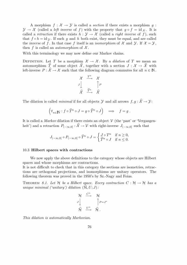
A morphism f : X → Y is called a section if there exists a morphism g :Y → X (called a left inverse of f ) with the property that g f = id X . It iscalled a retraction if there exists h : Y → X (called a right inverse of f ), suchthat f h = id Y . If such g and h both exist, they must be equal, and are calledthe inverse of f . In that case f itself is an isomorphism of X and Y . If X = Y ,then f is called an automorphism of X .

With this terminology we may now define our Markov chains.

Definition. Let T be a morphism X → X . By a dilation of T we mean anautomorphism T of some object X , together with a section J : X → X withleft-inverse P : X → X such that the following diagram commutes for all n ∈ IN.

X Tn

−→ XJ

yxP

X Tn

−→ X

The dilation is called minimal if for all objects Y and all arrows f, g : X → Y :

(∀n∈IN : f Tn J = g Tn J

)=⇒ f = g .

It is called a Markov dilation if there exists an object V (the ‘past’ or ‘Vergangen-

heit’) and a retraction P(−∞,0] : X → V with right-inverse J(−∞,0] such that

J(−∞,0] P(−∞,0] Tn J =

J Tn if n ≥ 0,Tn J if n ≤ 0.

10.3 Hilbert spaces with contractions

We now apply the above definitions to the category whose objects are Hilbertspaces and whose morphisms are contractions.It is not difficult to check that in this category the sections are isometries, retrac-tions are orthogonal projections, and isomorphisms are unitary operators. Thefollowing theorem was proved in the 1950’s by Sz.-Nagy and Foias.

Theorem 8.1. Let H be a Hilbert space. Every contraction C : H → H has aunique minimal (‘unitary’) dilation (H, U ; J) :

H Cn

−→ HJ

yxP=J∗

H Un

−→ H .

This dilation is automatically Markovian.

76

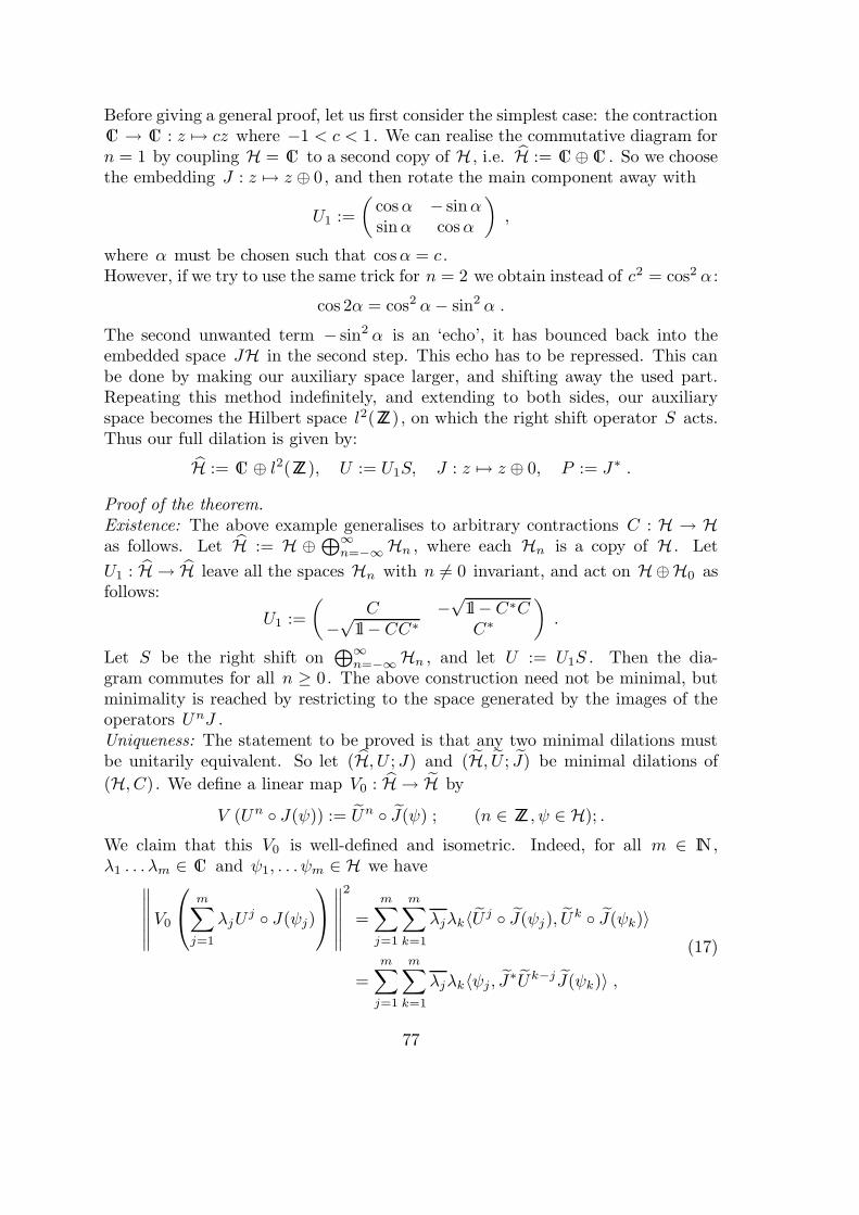
Before giving a general proof, let us first consider the simplest case: the contractionC → C : z 7→ cz where −1 < c < 1. We can realise the commutative diagram forn = 1 by coupling H = C to a second copy of H , i.e. H := C ⊕ C . So we choosethe embedding J : z 7→ z ⊕ 0, and then rotate the main component away with

U1 :=

(cosα − sinαsinα cosα

),

where α must be chosen such that cosα = c .However, if we try to use the same trick for n = 2 we obtain instead of c2 = cos2 α :

cos 2α = cos2 α− sin2 α .

The second unwanted term − sin2 α is an ‘echo’, it has bounced back into theembedded space JH in the second step. This echo has to be repressed. This canbe done by making our auxiliary space larger, and shifting away the used part.Repeating this method indefinitely, and extending to both sides, our auxiliaryspace becomes the Hilbert space l2(ZZ), on which the right shift operator S acts.Thus our full dilation is given by:

H := C ⊕ l2(ZZ), U := U1S, J : z 7→ z ⊕ 0, P := J∗ .

Proof of the theorem.Existence: The above example generalises to arbitrary contractions C : H → Has follows. Let H := H ⊕⊕∞

n=−∞Hn , where each Hn is a copy of H . Let

U1 : H → H leave all the spaces Hn with n 6= 0 invariant, and act on H⊕H0 asfollows:

U1 :=

(C −

√1l− C∗C

−√

1l− CC∗ C∗

).

Let S be the right shift on⊕∞

n=−∞Hn , and let U := U1S . Then the dia-gram commutes for all n ≥ 0. The above construction need not be minimal, butminimality is reached by restricting to the space generated by the images of theoperators UnJ .Uniqueness: The statement to be proved is that any two minimal dilations mustbe unitarily equivalent. So let (H, U ; J) and (H, U ; J) be minimal dilations of

(H, C). We define a linear map V0 : H → H by

V (Un J(ψ)) := Un J(ψ) ; (n ∈ ZZ , ψ ∈ H); .

We claim that this V0 is well-defined and isometric. Indeed, for all m ∈ IN,λ1 . . . λm ∈ C and ψ1, . . . ψm ∈ H we have

∥∥∥∥∥∥V0

m∑

j=1

λjUj J(ψj)

∥∥∥∥∥∥

2

=

m∑

j=1

m∑

k=1

λjλk〈U j J(ψj), Uk J(ψk)〉

=

m∑

j=1

m∑

k=1

λjλk〈ψj, J∗Uk−j J(ψk)〉 ,

(17)

77

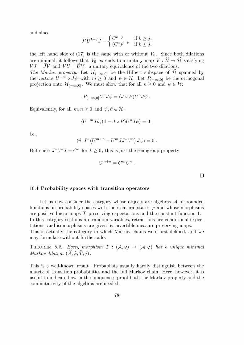
and since

J∗Uk−j J =

Ck−j if k ≥ j,(C∗)j−k if k ≤ j,

the left hand side of (17) is the same with or without V0 . Since both dilations

are minimal, it follows that V0 extends to a unitary map V : H → H satisfyingV J = JV and V U = UV : a unitary equivalence of the two dilations.The Markov property: Let H(−∞,0] be the Hilbert subspace of H spanned bythe vectors U−m Jψ with m ≥ 0 and ψ ∈ H . Let P(−∞,0] be the orthogonalprojection onto H(−∞,0] . We must show that for all n ≥ 0 and ψ ∈ H :

P(−∞,0]UnJψ = (J P )UnJψ .

Equivalently, for all m,n ≥ 0 and ψ, ϑ ∈ H :

〈U−mJϑ, (1l− J P )UnJψ〉 = 0 ;

i.e.,

〈ϑ, J∗ (Um+n − UmJJ∗Un)Jψ〉 = 0 .

But since J∗UkJ = Ck for k ≥ 0, this is just the semigroup property

Cm+n = CmCn .

10.4 Probability spaces with transition operators

Let us now consider the category whose objects are algebras A of boundedfunctions on probability spaces with their natural states ϕ and whose morphismsare positive linear maps T preserving expectations and the constant function 1.In this category sections are random variables, retractions are conditional expec-tations, and isomorphisms are given by invertible measure-preserving maps.This is actually the category in which Markov chains were first defined, and wemay formulate without further ado:

Theorem 8.2. Every morphism T : (A, ϕ) → (A, ϕ) has a unique minimal

Markov dilation (A, ϕ, T ; j) .

This is a well-known result. Probablists usually hardly distinguish between thematrix of transition probabilities and the full Markov chain. Here, however, it isuseful to indicate how in the uniqueness proof both the Markov property and thecommutativity of the algebras are needed.

78

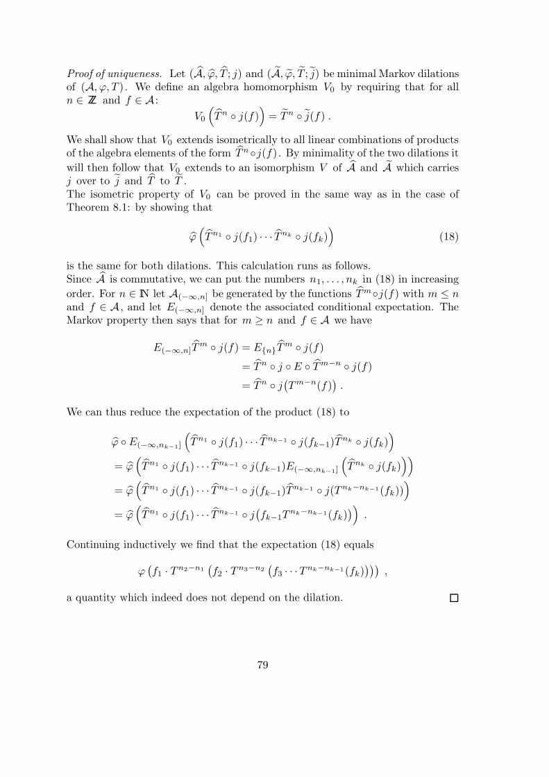
Proof of uniqueness. Let (A, ϕ, T ; j) and (A, ϕ, T ; j) be minimal Markov dilationsof (A, ϕ, T ). We define an algebra homomorphism V0 by requiring that for alln ∈ ZZ and f ∈ A :

V0

(Tn j(f)

)= Tn j(f) .

We shall show that V0 extends isometrically to all linear combinations of productsof the algebra elements of the form Tnj(f). By minimality of the two dilations it

will then follow that V0 extends to an isomorphism V of A and A which carriesj over to j and T to T .The isometric property of V0 can be proved in the same way as in the case ofTheorem 8.1: by showing that

ϕ(Tn1 j(f1) · · · Tnk j(fk)

)(18)

is the same for both dilations. This calculation runs as follows.Since A is commutative, we can put the numbers n1, . . . , nk in (18) in increasing

order. For n ∈ IN let A(−∞,n] be generated by the functions Tmj(f) with m ≤ nand f ∈ A , and let E(−∞,n] denote the associated conditional expectation. TheMarkov property then says that for m ≥ n and f ∈ A we have

E(−∞,n]Tm j(f) = EnT

m j(f)

= Tn j E Tm−n j(f)

= Tn j(Tm−n(f)

).

We can thus reduce the expectation of the product (18) to

ϕ E(−∞,nk−1]

(Tn1 j(f1) · · · Tnk−1 j(fk−1)T

nk j(fk))

= ϕ(Tn1 j(f1) · · · Tnk−1 j(fk−1)E(−∞,nk−1]

(Tnk j(fk)

))

= ϕ(Tn1 j(f1) · · · Tnk−1 j(fk−1)T

nk−1 j(Tnk−nk−1(fk)))

= ϕ(Tn1 j(f1) · · · Tnk−1 j

(fk−1T

nk−nk−1(fk)))

.

Continuing inductively we find that the expectation (18) equals

ϕ(f1 · Tn2−n1

(f2 · Tn3−n2

(f3 · · ·Tnk−nk−1(fk)

))),

a quantity which indeed does not depend on the dilation.

79