Friedrich–Alexander–Universität Erlangen–NürnbergDepartment für PhysikLehrstuhl für Theoretische Physik IProf. Dr. Ana-Sunčana Smith

Quantum Physics

Collection of problems

This is a collection of problems in quantum mechanics for undergraduate physics students, puttogether by Prof. Dr. Ana-Sunčana Smith and her group at FAU Erlangen–Nürnberg.

Many of these exercises were collected from materials presented over the years at Friedrich-Alexander-University Erlangen-Nürnberg, Germany and University of Zagreb, Croatia. Some ofthe exercises were conceived by Prof. Dr. T. Franosch (University of Innsbruck, Austria), Prof.Dr. T. Nikšić (University of Zagreb, Croatia) and the authors of the script.

All users of this collection are requested to kindly report any errors and omissions to SmithGroup at FAU Erlangen-Nürnberg, in particular to Mislav Cvitković or Robert Blackwell.

1

1 Introduction and Analogies

Problem 1.1 Delta function

a) The δ-function can be represented as the limit, as N −→∞, of the sum

N∑k=−N

e2πikx .

Show the above sum is equal to

f(x) =sin[2π(N + 1

2)x]sin(πx) (1.1)

for x 6= 0. Hint: Use Euler’s formula and the identity

2N∑k=0

zk = z2N+1 − 1z − 1 .

The 3-dimensional δ-function can be analogously represented as

limN→∞

N∑h=−N

N∑k=−N

N∑l=−N

e2πi(hx+ky+lz) .

Show for x, y, z 6= 0, the above sum is equal to f(x)f(y)f(z) where f(x) is as defined in(1.1).

b) Evaluate the following integrals:(i) ˆ 3

0x3 δ(x+ 1) dx

(ii) ˆ 1

−19x2 δ(3x+ 1) dx

(iii) ˆV ′

(r2 + 2) ∇ ·(err2

)dV,

where V ′ is a sphere of radius R centred at the origin, and er is the unit vector inthe radial direction. Hint: Use the fact that ∇ ·

(err2

)= 4πδ3(r).

(iv) ˆV ′|r− b|2 δ3(5r) dV,

where V ′ is a cube of side 2, centred on the origin, and b = 4ey + 3ez.

2

Problem 1.2 Spherical harmonics

a) The ‘associated’ Legendre polynomials Pml

Pml (x) = (−1)m

2ll! (1− x2)m/2 ∂l+m

∂xl+m(x2 − 1)l

can be calculated for −l ≤ m ≤ l. Verify that for l = 0, ..., 3 they fulfil the differentialequation

∂

∂x

[(1− x2)∂P

ml (x)∂x

]+[l(l + 1)− m2

1− x2

]Pml (x) = 0 .

b) The spherical harmonics Ylm(ϑ, ϕ) are defined by

Ylm(ϑ, ϕ) =

√√√√2l + 14π

(l −m)!(l +m)!P

ml (cosϑ)eimϕ .

Verify for l, l′ ≤ 2 the orthonormality conditionˆ 2π

0dϕˆ π

0sinϑ dϑ Y ∗l′m′(ϑ, ϕ)Ylm(ϑ, ϕ) = δll′δmm′ .

Problem 1.3 Eikonal Equation and Fermat’s Principle

The refractive index in the atmosphere varies weakly in space and may be approximated by alinear change with respect to the z-axis

n(z) = n(0)− z n′(0), n(0) > 0, n′(0) > 0,

where n(0) corresponds to the refractive index at ground level. The problem is to be discussedin the limit of geometrical optics, where for the wavelength of the ray λn′(z) 1 is valid.

Fig. 1: Scheme of the light trajectory.

a) Calculate the trajectory of a light ray in the atmosphere (see fig. 1). Use the equationsof the method of characteristics (ray equations) for the eikonal equation to determinex(`), z(`) as a function of the flow parameter `. Eliminate ` in favor of x to obtain adescription for the trajectory z(x).

3

b) In addition determine z(x) relying on Fermat’s principle by minimizing the optical path

S =ˆnds.

Use the methods of Euler-Lagrange to obtain a description for z(x).

Problem 1.4 Electromagnetic Wave as Analogy to Quantum Matter Waves

Consider an electromagnetic monochromatic plane wave propagating in vacuum ε = 1 and µ = 1with a wave vector k = (0, 0, k). The electric field vector should oscillate in time and space withE(r, t) = (0, 0, Ez(x, t)) where Ez(x, t) = exp[i(kx− ωt)] for a given frequency ω. At positionx = 0 a dielectric medium fills the half space x > 0, which is characterized by ε ≥ 1 and µ = 1.The medium is assumed to be transparent, so ε is real. A part of the wave is transmitted throughthe dielectric medium.

Fig. 2: Scheme of reflection.

a) What can be inferred on the the frequencies ω′ for the transmitted wave?b) The stationary electric field has to fulfill the wave equation,[

ε(x)ω2

c2 + d2

dx2

]Ez(x) = 0,

which is a one dimensional problem only. Discuss the following ansatz for the solutions

Ez(x) =

eikx + r e−ikx for x < 0,t eik′x for x > 0

c) Write down the dispersion relations for x < 0 and x > 0.d) Use the continuity conditions for the fields at the interface to express the amplitudes in

terms of ε.e) Calculate the transmission coefficient T and the reflection coefficient R. Show, thatT +R = 1.

Problem 1.5 Tunnel Effect

Consider a thin film of thickness 2a characterized by a dielectric constant εm dividing thethree-dimensional space (dielectric constant ε); see fig. 1.5. A monochromatic electromagneticplane wave is incident on the film. Choose a coordinate system such that the incident wavevector reads ki = (k, k‖, 0). Discuss the case of a polarization of the incident electric field parallelto the interfaces, Ei = (0, 0, Ei).

4

Fig. 3: Scheme of the Problem 1.5.

a) Determine the dispersion relation ω = ω(k) separately in each region.b) Argue that the polarization of the electric field is parallel to the interface in all three

regions.c) Since the tangential component of the electric field is continuous at the interfaces, the

spatio-temporal modulation at the interface are identical. Justify the following ansatz forthe electric field

Ez(x, t) = ei k‖y−iωt

Eiei kx + Ere− i kx for x < −a,E+ei qx + E−e− i qx for −a < x < a,

Etei kx for x > a ,

and interpret the individual terms. Show that q becomes purely imaginary for k2‖ >

εmω2/c2.

d) Establish the conditions of continuity for the tangential components of H (= B here)and calculate the effective transmission amplitude t = Et/Ei and the effective reflectionamplitude r = Er/Ei.

Problem 1.6 Paraxial Beams

Consider a monochromatic electromagnetic beam of angular frequency ω = ck propagatingessentially along the positive z-direction.

a) Argue that the components of the electric field allow for a representation as

E(x⊥, z; t) = e− iωtˆ d2k⊥

(2π)2 a(k⊥) exp(i k⊥x⊥ + i k‖z) ,

where k‖ = (k2 − k2⊥)1/2 is to be eliminated in favor of k⊥.

b) The complex amplitudes a(k⊥) are assumed to contribute only for |k⊥| k. Expandingthe square root, k‖ ' k − k2

⊥/2k to leading order in k⊥/k, show that the field assumesthe following form

E(x⊥, z; t) = ei kz−iωtE(x⊥, z) ,where the envelope function E is slowly varying along z on the scale of a wavelength,∂zE kE . Relate the envelope to the amplitudes a(k⊥). Show that the envelope satisfiesa field equation of the Schrödinger type,

i ∂zE(x⊥, z) = − 12k∇

2⊥E(x⊥, z).

In particular, the field equation is first order in the z-direction.

5

c) Evaluate the electric field E(x⊥, z; t) for a Gaussian amplitude function

a(k⊥) ∝ exp(−1

4w20k

2⊥

), w0 > 0 ,

and show that the intensity I ∝ |E|2 exhibits a Gaussian profile in the perpendiculardirection x⊥ and a width that depends on z. Where is the width minimal?

Problem 1.7 Angular Momentum Conservation Law

The angular momentum density of the electromagnetic field is defined by the antisymmetrictensor field

Lij(x, t) = 1c2 (xiSj − xjSi) ,

where S denotes the Poynting vector.a) Employ the momentum balance law to construct a local balance law for the angular

momentum density of the form

∂tLij +∇kMijk = −Dij .

Determine the angular moment current tensor Mijk as well as the mechanical torquetensor Dij. Rewrite the balance law in terms of the pseudo-vector field

Li(x, t) = 12εijkLjk ,

and suitable Mik and Di.b) Formulate the angular momentum conservation law in integral form, for Li =

´VLi dV .

c) Demonstrate that in the gauge ϕ = 0, the angular momentum of the field can bedecomposed, L = LS + LB, in a ‘spin’ part

LS = 14πc2

ˆV

A× A dV ,

and an ‘orbital’ part LB that depends explicitly on the point of reference of the coordinatesystem.

Problem 1.8 Radiation Loss of a Harmonically Oscillating Charge

a) A positive charge is attached to a spring (Fig. 6) in such a way that a radiating harmonicoscillator results. Show that small radiation losses with a minor reaction on a motion ofthe oscillator may be described by introducing a frictional force proportional to the thirdderivative of the elongation.

b) Consider an isolated system which emits dipole radiation mainly with the frequency ω0.Due to the radiation, the energy of the system is diminished permanently. This impliesthat the frequencies ω = ω0 + ∆ω adjacent to ω0 are emitted by the system. ∆ω is calledthe natural width of the emission line. Show that for a radiating harmonic oscillatorof mass m and charge e, in case of weak damping, the natural line width is given by∆ω = 2

3e2ω2

0mc3

.

6

Fig. 6: A charge attached to a spring.

Problem 1.9 Linear Response to the Field — Lorentz–Drude Model

Consider the constitutive equation of the Lorentz–Drude model,

∂2t P(x, t) + 1

τ∂tP(x, t) + ω2

0P(x, t) =ω2p

4πE(x, t) ,

with the relaxation time τ , characteristic frequency ω0 and the plasma frequency ωp.a) Perform a spatio-temporal Fourier transform and determine the complex susceptibilityχ(ω), with P(k, ω) = χ(ω)E(k, ω), as well as the dielectric function ε(ω) = 1 + 4πχ(ω).

b) Argue that the longitudinal modes follow from the zero of the dielectric function, ε(ω∗) = 0,and determine the complex frequency ω∗ in the case of weak damping.

c) Ignoring the damping (i.e. τ →∞) determine the dispersion relation of the transversemodes.

d) Explain without calculation, in what frequency regime the damping is most important.

Problem 1.10 Classical Hydrogen Atom, s–orbitals

Quantum mechanics reveals that the electron in a hydrogen atom should be described interms of a wave function ψ(r) (probability amplitude) giving rise to a smeared electron cloudcorresponding to a charge density, ρe(r) = −e|ψ(r)|2. At the center of the atom, the proton islocalized at a much smaller length scale, and the contribution to the charge density may bemodelled as a point charge, eδ(r). Determine the (total) electrostatic potential ϕ

a) for the (1s–orbital, K–shell) ground state of the hydrogen atom. Here the wave functionis spherically symmetric

ψ(r) = 1√πa3

e−r/a

where a = ~2/2me2 = 0.529× 10−8cm denotes the Bohr radius.b) for the spherically symmetric first excited state (2s–orbital, L–shell)

ψ(r) = 1√8πa3

(1− r

2a

)e−r/2a .

7

Problem 1.11 Classical Hydrogen Atom, p–orbitals

The electronic charge distribution of a hydrogen atom in a p–orbital has the following form inspherical coordinates

ρ(r) = − e

64πa3

(r

a

)2e−r/a sin2 ϑ

where a is the Bohr radius and e is the elementary charge.a) Calculate the multipole moment

qlm =ˆR3Y ∗lm(ϑ′, ϕ′)r′lρ(r)dV ′

and the multipole expansion

Φ(r) :=∑l,m

4π2l + 1

qlmrl+1Ylm(ϑ, ϕ).

Hint: sin2 ϑ can be expressed as a linear combination of spherical harmonics.b) How and why is Φ different from the exact potential

Φ(r) =ˆR3

ρ(r′)|r− r′|

dV ′ ?

Hint: You may use the following relation

1|r− r′|

=∞∑l=0

l∑m=−l

4π2l + 1

rl<rl+1>

Ylm(ϑ, ϕ)Y ∗lm(ϑ′, ϕ′) ,

where r>(r<) denotes absolute value of the larger (smaller) of the two radius vectors rand r′.

c) What is the behaviour of Φ(r) for r a?

Problem 1.12 Gaussian Wave Packet — Heisenberg’s Uncertainty Relation

Consider a particle that is described by the wave function

ψ(x) = Ae−x24a2

where a is real and positive.a) Normalize the wave function.b) Calculate 〈x〉, 〈p〉, 〈x2〉, 〈p2〉.c) Evaluate the product of the standard deviations σxσp. Compare it to Heisenberg’s

uncertainty relation σxσp ≥ ~/2.

8

2 Algebra, Operators, Representations

Problem 2.1 Hilbert Space

a) For what range of ν is the function f(x) = xν in Hilbert space, on the interval (0, 1)?Assume ν is real, but not necessarily positive.

b) For the specific case ν = 1/2, is f(x) in Hilbert space? What about xf(x)? How about(d/dx)f(x)?

Problem 2.2 Commutator Rules

Show the following relations for the commutator [A,B] of the two linear operators A, B:a) [A, [B,C]] + [B, [C,A]] + [C, [A,B]] = 0 (Jacobi rule).b) [AB,C] = A[B,C] + [A,C]B (Leibnitz rule).c) [A, [A,B]] = 0 ⇒ [An, B] = nAn−1[A,B], ∀n ∈ N.d) f(x) = ∑∞

n=0 anxn and [A, [A,B]] = 0 ⇒ [f(A), B] = f ′(A)[A,B].

Problem 2.3 Dirac Notation

Consider the three-dimensional Hilbert space spanned by the orthonormal basis |1〉, |2〉, |3〉.Two kets are given: |α〉 = i|1〉 − 4|2〉 − 2i|3〉, |β〉 = 2i|1〉+ 2|3〉.

a) Write down 〈α| and 〈β|. Calculate 〈α|α〉, 〈β|β〉, 〈β|α〉 and 〈β|α〉. Verify 〈β|α〉 = 〈α|β〉∗.b) What are the matrix elements of the operator A = |α〉〈β| in the basis |1〉, |2〉, |3〉.c) Find the energy eigenvalues and the corresponding eigenkets for a system characterized by

the Hamiltonian H = a (|2〉〈1|+ |1〉〈2|+ 2|3〉〈3|). Don’t forget to normalize your result.

Problem 2.4 Bra-Ket Trainer

Let |ai〉 : i = 1, ..., N ∈ N and |bi〉 : i = 1, ..., N ∈ N be two different complete sets oforthonormal vectors, which span the N -dimensional complex Hilbert space H.

|aj〉 =N∑i=1

Uij|bi〉, where Uij = 〈bi|aj〉.

Use the bra-ket notation to solve the following exercises:a) Show that the operator

U :=∑i,k

|ai〉〈bi|ak〉〈ak| =∑i,k

|ai〉Uik〈ak|

fulfills |ai〉 = U |bi〉 ∀ i = 1, ..., N . Show that U is unitary, meaning U †U = 1.b) For any linear operator A show that tr(A) := ∑

i〈ai|A|ai〉 does not depend on the choiceof the basis, i.e. show tr(A) = ∑

i〈bi|A|bi〉.

9

Problem 2.5 Adjoint and Hermitian Operators

The scalar product with some operator A is defined as

(ϕ,Aψ) =ˆϕ∗(r)Aψ(r) dr.

The adjoint operator is called A†, if

(ϕ,Aψ) =(A†ϕ, ψ

)or equivalently ˆ

ϕ∗(r)Aψ(r) dr =ˆ (

A†ϕ(r))∗ψ(r)dr.

a) Determine the adjoint operator of the operator αA, α ∈ C.b) Show, that for two Hermitian operators αA+ βB is Hermitian, if α, β ∈ R.c) Prove, that the momentum operator P = ~

i ∇ is Hermitian.d) What is the adjoint operator to the product operator C = AB, which is defined as

Cψ(r) = (AB)ψ(r) = A(Bψ(r)).

If A and B are Hermitian, when is AB Hermitian?e) Show, that H = − ~2

2m∆ + V (Q) and L = Q× ~i ∇ (only one component) are Hermitian.

Problem 2.6 Properties of the Hermitian Operators

a) Show that the sum of two Hermitian operators is Hermitian.b) Suppose Q is Hermitian, and α is a complex number. Under what condition on α is αQ

Hermitian?c) When is the product of two Hermitian operators Hermitian?d) Show that the position operator (x = x) and the Hamiltonian operator

H = − ~2

2md2

dx2 + V (x)

are Hermitian.e) Show that the eigenvalues of Hermitian operator are real.f) Show that if 〈h|Qh〉 = 〈Qh|h〉 for all functions h (in Hilbert space), then 〈f |Qg〉 = 〈Qf |g〉

for all f and g.

Problem 2.7 Probability Current

Max Born first suggested that the mod-square of a particle’s wave function

ρ(x, t) ≡ |Ψ(x, t)|2

is the probability density of finding the particle near x at time t. Since the particle is certain tobe found somewhere at each instant of time t, for this interpretation to make sense we must haveˆ

|Ψ(x, t)|2 d3x = 1. (2.3)

10

a) Defining the probability current J as

J(x) = i~2m (Ψ∇Ψ∗ −Ψ∗∇Ψ)

show that the following continuity equation is satisfied:

∂ρ

∂t= −∇ · J.

b) With the help of the continuity equation, show that

ddt

ˆ

all space

ρ d3x = 0

showing that eq. (2.3) is indeed satisfied.c) Writing Ψ as

Ψ(x) = S(x)eiϕ(x)

with S and ϕ real, show that the velocity v of the probability current, defined as J = ρv,is

v = ~∇ϕ

m.

Problem 2.8 Ladder Operators

a) Let B = cA + sA†, where c ≡ coshϑ, s ≡ sinhϑ with ϑ a real constant and A, A† arethe usual ladder operators. Show that [B,B†] = 1.

b) Consider the Hamiltonian

H = εA†A+ 12λ(A†A† + AA) ,

where ε and λ are real and such that ε > λ > 0. Show that when

εc− λs = Ec ; λc− εs = Es

with E a constant, [B,H] = EB. Hence determine the spectrum of H in terms of ε andλ.

Problem 2.9 Fermi Oscillator

A Fermi oscillator has the Hamiltonian H = f †f , where f is an operator that satisfies

f 2 = 0; ff † + f †f = 1 .

Show that H2 = H, and thus find the eigenvalues of H. If the ket |0〉 satisfies H|0〉 = 0 with〈0|0〉 = 1, what are the kets |a〉 ≡ f |0〉, and |b〉 ≡ f †|0〉?In quantum field theory the vacuum is pictured as an assembly of oscillators, one for eachpossible value of the momentum of each particle type. A boson is an excitation of a harmonicoscillator, while a fermion is an excitation of a Fermi oscillator. Explain the connection betweenthe spectrum of f †f and the Pauli principle.

11

Problem 2.10 Baker-Hausdorff Identity

Prove that for two operators A, B and a complex parameter y, the so-called Baker-Hausdorffidentity

eyABe−yA = B + y[A,B] + y2

2! [A, [A,B]] + ...+ yn

n! [A, [A, ..[A,B]...]]n + ...

holds. Hint: Define F (y) = eyABe−yA and consider dFdy.

Problem 2.11 Translation Operator

a) In this problem you derive the wavefunction

〈x|p〉 = eip·x/~ (2.6)

of a state of well defined momentum for the properties of the translation operator U(a).The state |k〉 is one of well-defined momentum ~k. How would you characterise thestate |k′〉 ≡ U(a)|k〉 ? Show that the wavefunctions of these states are related byuk′(x) = e−ia·kuk(x) and uk′(x) = uk(x− a). Hence obtain equation (2.6).

b) The relation [vi, Jj] = i∑k εijkvk holds for any operator whose components vi form a

vector. The expectation value of this operator relation in any state |ψ〉 is then

〈ψ|[vi, Jj]|ψ〉 = i∑k

εijk〈ψ|vk|ψ〉.

Check that with U(α) = e−iα·J this relation is consistent under a further rotation|ψ〉 → |ψ′〉 = U(α)|ψ〉 by evaluating both sides separately.

Problem 2.12 Rotation Operator

a) Show that the vector product a×b of two classical vectors transforms like a vector underrotations. Hint: A rotation matrix R satisfies the relations R ·RT = I and det(R) = 1,which in tensor notation read ∑pRipRtp = δit and

∑ijk εijkRirRjsRkt = εrst.

(i) Let the matrices Jx, Jy and Jz be such that exp(−iα · J) ≡ R(α), where theexponential of a matrix is defined in terms of the power series for ex. Here α is avector that specifies a rotation through an angle |α| around the direction of the unitvector α. Show that Ji are Hermitian matrices.

(ii) Show that for any two vectors α and β the product RT (α)R(β)R(α) is an orthogonalmatrix with determinant +1, so it is a rotation matrix.

(iii) Make a Taylor expansion of exp(−iα · J) ≡ R(α) for small |α| and |β| and show[Ji, Jj] = i

∑k εijkJk.

b) Show that if α and β are non-parallel vectors, α is not invariant under the combined rota-tion R(α)R(β). Hence show that RT (β)RT (α)R(β)R(α) is not the identity operation.Explain the physical significance of this result.

c) The matrix for rotating an ordinary vector by ϕ around the z axis is

R(ϕ) ≡

cosϕ − sinϕ 0sinϕ cosϕ 0

0 0 1

.By considering the form taken by R for infinitesimal ϕ calculate from R the matrix Jz thatappears in R(ϕ) = exp(−iJzϕ). Introduce new coordinates u1 ≡ (−x+ iy)/

√2, u2 = z

12

and u3 ≡ (x+ iy)/√

2. Write down the matrix M that appears in u = M · x [where x ≡(x, y, z)] and show that it is unitary. Then show that

J′z ≡M · Jz ·M† (2.7)is identical with Sz in the set of spin-one Pauli analogues

Sx = 1√2

0 1 01 0 10 1 0

, Sy = 1√2

0 −i 0i 0 −i0 i 0

, Sz =

1 0 00 0 00 0 −1

. (2.8)

Write down the matrix Jz whose exponential generates rotations around the x axis,calculate J′x by analogy with equation (2.7) and check that your result agrees with Sz inthe set (2.8). Explain as fully as you can the meaning of these calculations.

Problem 2.13 Shift Operator and Heisenberg Algebra

Let Ψ : R→ C be an arbitrary wavefunction. The shift operator Ta, a ∈ R, is defined through(TaΨ)(x) = Ψ(x+ a).

Let Ψ : R3 → C be an arbitrary wavefunction. The momentum and position operatorsPi, Qi (i = 1, 2, 3) are defined as following:

(QiΨ)(r) = riΨ(r),

(PiΨ)(r) = ~i∂

∂riΨ(r),

a) Express Ta in terms of the momentum operator P = ~i∂∂x.

b) Calculate all commutators [Qi, Qj], [Pi, Pj], [Qi, Pj], i, j = 1, 2, 3.c) Calculate [Q,P ], [Q,H], [P,H] for the Hamiltonian of the harmonic oscillator:

H = 12mP 2 + mω2

2 Q2.

3 Dynamics, Time Evolution

Problem 3.1 Localized Particle

Consider a free particle that is localized in the range −a < x < a at time t = 0:

ψ(x, 0) =

A, if − a < x < a;0, otherwise.

a) Normalize the given wave function and calculate its representation in momentum spaceψ(k, 0).

b) Discuss and compare ψ(x, 0) versus ψ(k, 0) for the two limiting cases of very small andvery large a. Interpret your result in terms of Heisenberg uncertainty principle.

c) Derive an expression to calculate the wave function ψ(x, t) for later times t in terms ofψ(k, 0).

13

Problem 3.2 Time Evolution of Superposition States

At time t = 0 a particle is assumed to be in a superposition of two stationary states ψ0, ψ1 withenergies E0, E1, respectively:

ψ(x, 0) = c0ψ0(x) + c1ψ1(x).

a) What is the wave function ψ(x, t) at later times? Calculate the probability density|ψ(x, t)|2. For simplicity assume that the coefficients c0, c1 as well as the wave functionsψ0, ψ1 are real.

b) What is the consequence of the interference between ψ0 and ψ1? Describe the motion of|ψ(x, t)|2. Compare this to the case c1 = 0.

c) Evaluate |ψ(x, t)|2 for the case of ψ0, ψ1 being the ground and first excited state of aparticle confined in an infinitely deep square well potential of width L and c0 = c1 = 1/

√2.

Problem 3.3 Evolution of Gaussian Wave Package

Consider a free particle described by a Gaussian wave package at time t = 0:

ψ(x, 0) = 1(2πa2)1/4 e

− x24a2 .

a) Find ψ(x, t) for later times t.b) Calculate the probability density and sketch |ψ|2 for t = 0. How does it evolve? How

does it look like for very large times?

Problem 3.4 Time Evolution, Conserved Observables

Consider an arbitrary time-dependent normalized wave function:

Ψ(t) :

R3 → C,r 7→ Ψ(r, t),ˆ

d3r |Ψ(r, t)|2 = 1, ∀t.

Let A be a time–independent linear operator (e.g. an operator corresponding to a physicalobservable) with [A,H] = 0.

a) Verify [An, H] = 0.b) Calculate d

dt〈An〉(t), where 〈An〉(t) is the expectation value of the operator An in the

state Ψ(t).

Problem 3.5 Ehrenfest Theorem and Quantum–Classical Correspondence

a) Show that [Q,F (P )] = i~∂F∂P

and [P,G(Q)] = −i~∂G∂Q

for any differentiable functions F (P )and G(Q).

14

b) Derive the Ehrenfest theorem,

md2

dt2 〈Q〉 = ddt〈P 〉 = −〈∇V (Q)〉 (3.1)

for any H = 12mP

2 + V (Q). Interpret it and relate it to Newton’s second law.c) The Poisson brackets for classical quantities f(p, q) and g(p, q) are defined as

f, g = ∂f

∂q

∂g

∂p− ∂f

∂p

∂g

∂q.

Show thatddtf(p, q) = f,H(p, q), (3.2)

where H(p, q) is the Hamiltonian of the classical system. What is the condition for f(p, q)to be a constant of motion?

d) Show that 1i~ [Q2, P 2] corresponds to q2, p2.

Problem 3.6 Virial Theorem

a) Prove that for any two differentiable functions of operators F and G (which are operators,too) and linear operators A and B which satisfy conditions: (i) [A, [A,B]] = 0, (ii)[B, [B,A]] = 0 and (iii) [[A,B], Bn] = 0 ∀n ∈ N the following relation is valid:

[F (A,B), G(A,B)] = ∂F

∂A

∂G

∂B[A,B] + ∂F

∂B

∂G

∂A[B,A],

which is generalisation of the Problem 2.2 d).b) Using a), show that the time derivative of function F (p, r), where p and r are momentum

and position operators, respectively, is given by commutator with Hamiltonian:

dF (p, r)dt = 1

i~ [F (p, r), H]

which is a quantum analogue to classical relation df/dt = f,H.c) Prove the virial theorem that formulates a general relation between the mean value of

the kinetic energy and the potential V (r):

2〈Ekin〉 = 〈r · ∇V (r)〉

and has the same form in classical and quantum physics.d) Show that for a spherically symmetric potential V (r) = Crα the mean kinetic energy is

directly given by mean potential energy:

2〈Ekin〉 = α〈V (r)〉.

15

Problem 3.7 Parity Operator and Quantum Zeno Effect

A quantum system is described by two energy eigenstates |1〉 and |2〉 with the correspondingenergies E1 and E2. Consider the parity operator P, which is acting on the eigenstates in thefollowing:

P|1〉 = |2〉, P|2〉 = |1〉.

a) Find the eigenstates of the parity operator and calculate the time evolution for the caseof being initially in the positive parity eigenstate |+〉.

b) At time t a parity measurement is made on the system. What is the probability tomeasure positive parity?

c) Imagine you make a series of parity measurements at the times ∆t, 2∆t, ..., N∆t = T ,where ∆t 1

ωand ω = E2−E1

2~ . What is the probability that the initially prepared positiveparity state survives at time T within that series of measurements? Investigate then thecase of N 1 and finally the limit N →∞ at constant T .

Problem 3.8 1D Quantum Well — Time Evolution

A particle (mass m) is confined in the infinite quantum well of the length L:

V (x) =

0, 0 < x < L,

∞, else.

The wave function at the time t = 0 reads

Ψ(x, 0) =

2b xL, 0 < x ≤ L

2 ,

2b(1− x

L

), L

2 < x < L.

a) Normalize the wavefunction (calculate b). Plot the probability density |Ψ(x, 0)|2

b) Using Schrödinger equation, calculate the wavefunction Ψ(x, t) at later times t > 0. Hint:Expand Ψ(x, 0) in the eigenbasis of the infinite quantum well. Use the orthonormality ofthe eigenstates ϕn:

〈un|ul〉 =ˆ L

0dx 〈un|x〉〈x|ul〉 =

ˆ L

0dxu∗n(x)ul(x) = δn,l.

c) Calculate the time-dependent expectation value of the energy, i.e. 〈H〉(t), in the stateΨ(t). You can use without proof

∑n=0

1(2n+ 1)2 = π2

8 .

Problem 3.9 Harmonic Oscillator — Galilei Invariance

Consider a particle in a quadratic potential that moves along the x-axis at constant speed:

H = 12mP 2 + k

2(Q− vt)2.

16

a) Transform into the reference frame moving with the potential by introducing the newvariables x = x− vt and t = t. Show that the Schrödinger equation can be rewritten as

i~(∂

∂t− v ∂

∂x

)Ψ(x, t) = − ~2

2m∂2

∂x2 Ψ(x, t) + k

2 x2Ψ(x, t). (3.10)

b) Eliminate the term ∂∂x

on the left hand side of (3.10) by introducing Ψ(x, t) = e−iα(x,t)Ψ(x, t).What are the solutions of the Schrödinger equation in the comoving frame and in thelaboratory frame?

c) Generalize the result of b): Assume you know the energy eigenstates Ψn(x) for a givenHamiltonian H = P 2/2m+ V (Q). Prove that

Φ(x, t) = e−i(E+mv22 )t/~eimvx/~Ψ(x− vt) (3.11)

is a solution of the Schrödinger equation for a particle subject to a moving potentialV (Q− vt).

Problem 3.10 Mößbauer Effect

We want to calculate the quantum-mechanical effects of a momentum transfer δp (e.g. fromemission, absorption, scattering, etc.) on a bound system. Consider a nucleus bound viathe potential V (Q). Before the absorbtion the nucleus is in the initial state |Ψin〉, whichis an (arbitrary) eigenstate of the Hamiltonian. Now the nucleus absorbs a photon with thewavenumber δk (i.e. momentum δp = ~δk). The new state |Ψnew〉 of the nucleus can be expressedas

|Ψnew〉 = N exp(

iδp~Q

)|Ψin〉,

where Q is the position operator and N a normalization constant.a) Calculate the normalization constant N .b) Convince yourself that |Ψnew〉 is an appropriate state to describe the momentum transfer:

Calculate the change of the expectation value of P and verify

δp = 〈Ψnew|P |Ψnew〉 − 〈Ψin|P |Ψin〉.

Hint: The action of Q in momentum space is QΨ(k) = i∂kΨ(k). Recall the shift operatorTa in coordinate space. What is its analogue in momentum space?

c) Calculate the change of the expectation value of the energy δE and compare it with theclassical expectation.

δE := 〈Ψnew|H|Ψnew〉 − 〈Ψin|H|Ψin〉.

d) Up to here we considered arbitrary potentials V (Q). Now we specialize to the case of theharmonic oscillator: V (Q) = mω2Q2/2. This can be regarded as a model for a nucleusbound on a lattice site of a crystal. The initial state |Ψin〉 is the ground state of theharmonic oscillator, i.e. |Ψin〉 = |0〉. Calculate the probability Pn := |〈n|Ψnew〉|2 for thenucleus to be in the n-th eigenstate of the harmonic oscillator after the absorbtion. Hint:You can use without proof the Baker-Campbell-Hausdorff identity:

[A, [A,B]] = [B, [A,B]] = 0 ⇒ exp(A+B) = exp(A) exp(B) exp(−1

2[A,B]).

What is the probability to stay in the ground state? What does it look like for small δp?

17

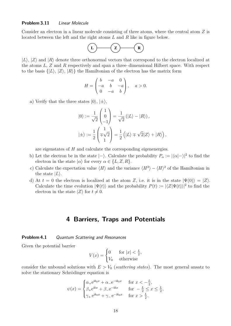
Problem 3.11 Linear Molecule

Consider an electron in a linear molecule consisting of three atoms, where the central atom Z islocated between the left and the right atoms L and R like in figure below.

RZL

|L〉, |Z〉 and |R〉 denote three orthonormal vectors that correspond to the electron localized atthe atoms L, Z and R respectively and span a three–dimensional Hilbert space. With respectto the basis |L〉, |Z〉, |R〉 the Hamiltonian of the electron has the matrix form

H =

b −a 0−a b −a0 −a b

, a > 0.

a) Verify that the three states |0〉, |±〉,

|0〉 := 1√2

10−1

= 1√2

(|L〉 − |R〉) ,

|±〉 := 12

1∓√

21

= 12(|L〉 ∓

√2|Z〉+ |R〉

),

are eigenstates of H and calculate the corresponding eigenenergies.b) Let the electron be in the state |−〉. Calculate the probability Pα := |〈α|−〉|2 to find the

electron in the state |α〉 for every α ∈ L,Z,R.c) Calculate the expectation value 〈H〉 and the variance 〈H2〉 − 〈H〉2 of the Hamiltonian in

the state |L〉.d) At t = 0 the electron is localized at the atom Z, i.e. it is in the state |Ψ(0)〉 = |Z〉.

Calculate the time evolution |Ψ(t)〉 and the probability P (t) := |〈Z|Ψ(t)〉|2 to find theelectron in the state |Z〉 for t 6= 0.

4 Barriers, Traps and Potentials

Problem 4.1 Quantum Scattering and Resonances

Given the potential barrier

V (x) =

0 for |x| < L2 ,

V0 otherwise

consider the unbound solutions with E > V0 (scattering states). The most general ansatz tosolve the stationary Schrödinger equation is

ψ(x) =

α+eik0x + α−e−ik0x for x < −L

2 ,

β+eikx + β−e−ikx for − L2 ≤ x ≤ L

2 ,

γ+ eik0x + γ− e−ik0x for x > L2 .

18

a) Relate the wave numbers in each region to the energy E.b) Formulate the continuity conditions for the above mentioned most general case and write

them as a matrix equations(α+α−

)=M

(k0, k,−

L

2

)(β+β−

)and

(β+β−

)=M

(k, k0,

L

2

)(γ+γ−

)

whereM(k0, k,−L2 ) ∈ K2×2 andM(k, k0,

L2 ) ∈ K2×2 are to be determined.

c) Express only the coefficients of |x| > L2 by each other, introduce new variables

ε+ = k

k0+ k0

kand ε− = k

k0− k0

k

and adapt the conditions γ− = 0, γ+ = S and α+ = 1, which describe the physicalsituation of an incoming quantum particle from x = −∞ which is scattered at thepotential. Determine S as a function of k, k0, ε−, ε+ and L.

d) Calculate the currents for the incident, reflected and transmitted wave: jI , jR, jT .e) Determine explicitly the transmission coefficient T . Find out the energies, for which

transmission is optimized. What is different between quantum and classical scattering inthis scenario?

Problem 4.2 Potential Barrier — Quantum Tunnelling

Consider again the one-dimensional motion of a particle that is incident on a potential barrier,V0 > 0,

V (x) =

V0 for 0 ≤ x ≤ d

0 else

a) Discuss the limit of thin and high barriers V0 → ∞, d → 0 such that the area V0d :=~2/2m` under the potential remains finite. Thus the potential barrier degenerates to

V (x) = ~2

2m`δ(x)

where δ(·) denotes the Dirac δ-distribution. The wavefunction remains continuous atx = 0 in this limit. Yet in the same limit, the derivatives exhibit a jump,

limx↓0

ψ′(x)− limx↑0

ψ′(x) = 1`ψ(0)

Show that the conditions can be obtained by inspecting the Schrödinger equation uponintegrating over a small interval containing the singularity. Discuss the transmissioncoefficient for the δ-potential.

Problem 4.3 Double Step Potential

A particle is incident from the left on the double potential step

V (x) =

0 for x < 0V0 for 0 ≤ x ≤ d

V1 for x > d

with 0 < V0 < V1 < E, where E denotes the energy of the particle. Calculate the reflection andtransmission amplitude. For what value of V0 and width d does the reflection vanish?

19

Problem 4.4 Double Well Oscillations

A particle of mass m and energy E < V0 moves in a one–dimensional potential box

V (x) =

∞ for |x| > b,

V0 for |x| < a,

0 for a < |x| < b.

as shown in the figure below:

∞

−b −a a b

∞

V0

V (x)

x

a) Solve the Schrödinger eq. and find the eigenvalues and an algebraic equation for eigenenergies of the system.

b) How does the potential define the number of states with E < V0?c) From the symmetry it is clear that system has well defined parity. Is the ground state

odd or even? Construct and sketch the wave functions of the first two states and theirsuperposition.

d) Calculate the time evolution for the case of being initially in the right well. There is someprobability to penetrate through the finite barrier. Can we ever be sure that we’ll findthe particle in the left well? If no, why? If yes, what time do we have to wait to haveparticle on the left?

Problem 4.5 Attractive δ–potential – Scattering and Bound States

Consider the one-dimensional stationary Schrödinger equation with the attractive delta potential

V (x) = − ~2

2m`δ(x),

where m denotes the mass of the particle and l > 0.a) Consider the scattering problem: A particle with energy E > 0 is incident from the left

on the potential. Use the ansatz

ψ(x) =

eikx + r e−ikx for x < 0,t eikx for x > 0,

and determine the wave number k, the coefficients r, t and the transmission amplitudeT = |t|2. Compare the results with those for the repulsive delta peak.

b) Solve the stationary Schrödinger equation for possible bound (localized) states, i.e. stateswith energy E < 0.

20

Problem 4.6 Double δ–function Potential

Consider the double delta-function potential

V (x) = −α(δ(x+ a) + δ(x− a)

),

where α and a are positive constants.a) Sketch this potential.b) How many bound states does it possess? Find the allowed energies for α = ~2/ma and

for α = ~2/4ma and sketch the wave functions.

Problem 4.7 Floquet’s Theorem

Solve the Schrödinger equation and find the allowed energies for a potential of the form

V (x) = ~2

mΩ

+∞∑n=−∞

δ(x+ na) .

Hint: First we have to prove the validity of the Floquet’s theorem, which says that if thepotential is periodic (V (x+ a) = V (x)), then ψ(x+ a) = eikaψ(x).

Problem 4.8 Periodic δ–comb — Eenergy Bands

Calculate possible eigenenergies of the one-dimensional Hamiltonian with the external potentialV corresponding to a periodic delta-comb:

V (x) = − ~2

2m`

∞∑n=−∞

δ(x− na)

Note: This problem can be interpreted as a simple model for a one-dimensional crystal withions fixed on positions na, n ∈ Z, and the single-ion potential − ~2

2m`δ(x).Let Ψ be a solution of the corresponding Schrödinger equation. By symmetry one argues thatthe electron density is periodic: |Ψ(x)|2 = |Ψ(x+ a)|2, meaning that the wavefunction itself isonly allowed to accumulate an arbitrary phase (Bloch theorem):

Ψ(x+ na) = einKaΨ(x), Ka ∈ [−π, π) arbitrary, n ∈ Z. (4.10)

Consider a plane-wave ansatz for x ∈ (0, a):

Ψ(x) = Aeikx +Be−ikx, x ∈ (0, a) .

a) Continue this ansatz to all regions ((n− 1)a, na) , n ∈ Z, such that the Bloch condition(4.10) is fulfilled. You should obtain

Ψ(x) = ei(n−1)Ka u [x− (n− 1)a] , for x ∈ ((n− 1)a, na) , n ∈ Z,u(x) = Aeikx +Be−ikx.

21

b) Write down the matching conditions for Ψ at x = a. What do the matching conditions atother points x = na look like? Rewrite the matching conditions in the form

M

(A

B

)= 0,

with a 2× 2 matrix M .c) Derive the condition for the matrix M in order for this linear equation to have nontrivial

solutions (A,B) 6= (0, 0). Check:

cos(Ka) = cos(ka)− a

2`sin(ka)ka

. (4.11)

d) Here we consider only solutions with positive energies, i.e. k ∈ R. Convince yourself —graphically — that Eq. (4.11) allows only for energies E (or wavevectors k) from certainintervals — these intervals are known as the energy bands of the crystal.

e) What are the allowed energies for a/` → ∞ and a/` → 0? At constant a/`, how doesthe width of the energy bands behave for increasing ak?

Problem 4.9 Bloch Bands

A simple model for a one–dimensional crystal with ions fixed on positions na, n ∈ Z, is thecomb of the single–ion potentials ~2Ω

mδ(x):

V (x) = ~2Ωm

∞∑n=−∞

δ(x+ na).

Using Bloch’s theorem

Ψ(x+ na) = einKaΨ(x), Ka ∈ [−π, π) arbitrary, n ∈ Z,

and plane–wave ansatz we have obtained in Problem 4.7 the condition (4.9) for energies:

cos (Ka) = cos (ka) + aΩsin (ka)ka

. (4.15)

a) Show (graphically) that (4.15) allows only for energies E (or wave vectors k) from certainintervals. These intervals are known as the energy bands of the crystal.

b) Plot the energy as a function of Ka. How does the width of the energy bands behave forincreasing k?

c) What are the allowed energies for aΩ→∞ and aΩ→ 0?

Problem 4.10 Separation of Variables in Axial Symmetry

Make a separation of variables for the Schrödinger equation in a potential that depends only onthe distance from the z-axis.

Problem 4.11 Particle Between Two Parallel Cylinders

The particle of mass m is in the space between two infinitely long concentric cylinders withradii r = a i r = b. The edge of every clyinder is an infinitely repulsive potential for the particle.Determine the energy and wave function of the particle in the ground, nρ = 0 state.

22

Problem 4.12 Finite Spherical Potential Well

A particle is in a spherical finite potential well of the form

V (r) =

−V0, r < a;0, r ≥ a.

Find the bound energy states for l = 0 and l = 1.

Problem 4.13 Spherical Shell

A particle of mass m moves in the space bounded by two concentric spheres with radii r< = aand r> = b. The sides of the spheres represent an infinite repelling potential for the particle.Calculate the energy and the wave function in the ground state (l = 0).

Problem 4.14 Landau levels

For a particle of mass m and charge Q in a magnetic field B, the Hamiltonian proves, fromrelativistic reasons, to be

H = 12m (p−QA)2

where A is the magnetic vector potential. For a particular case, let B = Bz, and chooseA = 1

2B(−y, x, 0)T .a) Express H in terms of pz and the dimensionless operators

πx ≡px + 1

2mωy√mω~

; πy ≡py − 1

2mωx√mω~

where ω = QB/m is the Larmor frequency. Show that H can be seen as the sum of thatof a free particle in one dimension and of that of a harmonic oscillator. Find the ladderoperators corresponding to the harmonic oscillator part of the Hamiltonian, and also thecorresponding energy levels (called Landau levels).

b) To find the wavefunction of a given Landau level, write down the ground state’s definingequation, A|0〉 = 0 (where A is the lowering ladder operator), in the position representation.Solve it to find 〈x|0〉 and subsequently 〈x|n〉.

c) In classical physics, a particle is not affected by an electromagnetic field that is restrictedto a region where the particle does not pass through. This is not so in quantum mechanics.

Consider an infinitely long and infinitely thin solenoid placed along the z-axis. Thereis a strong magnetic field B inside the solenoid, and, due to its infinite length, noneoutside it. Suppose a screen is placed along the plane y = 0, with two slits along thelines x = ±s. The screen is bombarded from the side y < 0 with particles that havewell-defined momenta p = py, and their arrival is detected on a screen P placed alongthe plane y = L. Show that the particles, which never enter the region of non-zero B, arestill affected by B.

23

Problem 4.15 Decomposition of Arbitrary Potential and α-decay

In the Problem 4.1 the transmission probability for a quantum particle at a finite potentialbarrier V0 of thickness L was determined.

a) Use the result and derive the transmission coefficient for the case E < V0, which is thetunnel effect through a constant barrier. Express all terms in favor of E and V0.

b) Find a convenient approximation for the case of a high and thick potential barrier, whichmeans κL 1. As a result one gets

T ≈ 16E(V0 − E)V 2

0exp

(−2~

√2m(V0 − E)L

).

In the limit of high potentials the tunnel probability is dominated by the exponential.Therefore the prefactor is neglected in the following.

c) To describe the transmission through a continuously varying potential, decompose thepotential within the classical forbidden area into N rectangular barrier segments of length∆x of the above described barrier type. Determine the transmission probability foreach segment i and then for the whole approximated potential. Assume as a furtherapproximation that no inner reflections occur. Finally apply the limit ∆x→ 0. Withinthis procedure, determine the Gamow factor G, defined as T ≈ exp(−G).

d) One of the most prominent applications of this formula is the α-decay. Consider a formedα-particle E > 0 moving within the center of a nucleus. Inside the alpha-particle feels aconstant negative potential coming from the nuclear interaction with the other nucleons.Beyond the average radius R of the nucleus the Coulomb potential VC(r) = γ

rforms a

finite potential barrier, which is classically impenetrable.

r

E

V0rc

V (r)

Here γ = 2Ze2/4πε0 and Z is the number of protons in the nucleus. Determine theclassical forbidden interval [R, rc]. Calculate the Gamow-factor and expand it in lowestorder for R/rc. Use the integral

rcˆ

R

dr√

1r− 1rc

= √rc

(π

2 − arcsin√R

rc−√R

rc

(1− R

rc

)).

Introduce fine–structure constant α = e2

4πε0~c and the common nuclear radius estimateR ≈ r0A

13 (with r0 = 1.2 fm and A being mass number). Express G in terms of Z, E, A

and α.e) The average life time of the state can be approximated with τ ≈ tnuc

T, where tnuc = 2R

vis

the time to move through the nucleus. Derive the so called Geiger–Nutall rule

ln τ ≈ c0 + c1Z√E

+ c2

√ZA

13

The explanation of the α-decay and the qualitative correct predictions of the average lifetimes could be seen as a big success of quantum mechanics.

24

Problem 4.16 Thomas–Reiche–Kuhn Sum Rules

Prove the so–called Thomas–Reiche–Kuhn sum rules for particle of mass m moving in a potentialV : ∑

j

|xij|2 (Ej − Ei) = ~2

2m and∑j

|pij|2 (Ej − Ei) = ~2

2

⟨∂2V

∂x2

⟩,

where Ei is the energy of state |i〉, xij ≡ 〈i|x|j〉 and pij ≡ 〈i|p|j〉.

4.1 Harmonic Oscillator

Problem 4.17 Harmonic Oscillator — Virial Theorem, Ground State, Uncertainty

a) Prove the quantum analogue of the virial theorem for a system with Hamiltonian H =1

2mP2 + V (Q)

d

dt〈QP 〉 = 1

m〈P 2〉 − 〈Q∇V (Q)〉. (4.26)

b) Now consider the special case of a harmonic oscillator, H = 12mP

2 + k2Q

2. What does thevirial theorem state? Show that, if the system is in an energy eigenstate (〈a†a〉 = n),

12m〈P

2〉 = k

2 〈Q2〉 = 1

2〈H〉 = ~ω2

(n+ 1

2

), (4.27)

where ω =√k/m.

c) Using the previous results, calculate the position-momentum uncertainty of a harmonicoscillator in the nth energy eigenstate.

Problem 4.18 Harmonic Potential

A particle is in the potential of a harmonic oscillator. For the first three eigenstates of theHamiltonian calculate the probability that the particle is in the classically forbidden region.

Problem 4.19 Harmonic Oscillator — Coherent States

The coherent state of the harmonic oscillator can be defined as the eigenstate of the annihilationoperator aϕα(ξ) = αϕα(ξ). The operator a = 1√

2(ξ+ ddξ ) is rescaled with respect to the oscillator

length x0 =√

~ωm

with ξ = xx0. The eigenvalue α of the annihilation operator a is complex, so

α = <α+ i=α = |α| exp(iδ).a) In opposite to the algebraic solution shown in the lecture directly determine ϕα(x) ≡ϕα( x

x0) via solving the differential equation.

b) Determine the dynamics ϕα(x, t) by assuming α→ α(t) and a time dependent prefactorN → N(t) concerning the above derived solution. Insert the ansatz into the timedependent Schrödinger equation and evaluate N(t) and α(t).

c) Normalize the wavefunction for t = 0 and calculate then |ϕα(x, t)|2. Which shape does ithave?

d) Calculate the expectation values 〈Q〉t, 〈P 〉t, 〈Q2〉t, 〈P 2〉t.e) Evaluate the product of the standard deviations σQσP . Compare it to Heisenberg’s

uncertainty relation σQσP ≥ ~/2.

25

Problem 4.20 Harmonic Oscillator — Energy Spectrum

We want to obtain all possible energies En and wavefunctions Ψn which obey

HΨn = EnΨn, where

H = 12mP 2 + mω2

2 Q2.

First we define the operators a†, a and express the momentum and coordinate in terms of a, a†:

a† :=√ωm

2~ Q− i√

12mω~P, a :=

√ωm

2~ Q+ i√

12mω~P,

⇒ Q =√

~2mω

(a+ a†

), P = i

√~ωm

2(a† − a

).

a) Verify [a, a†] = 1 (this means aa† = 1 + a†a).b) Use the expression of Q, P in terms of a†, a to verify

H = ~ω2(aa† + a†a

)= ~ω

(a†a+ 1

2

).

c) Using a) and b), verify Ha† = a† (H + ~ω).d) Now assume that Ψ is a solution of the stationary Schrödinger equation with the energyE, i.e. HΨ = EΨ. Use c) to show that a†Ψ is solution with the energy E ′ = E + ~ω.

e) Show that the Gaussian

Ψ0(x) =( 1

2πσ2

) 14

exp(−1

4x2

σ2

)

is a solution and calculate σ and the corresponding energy. Why is it the ground state?f) Starting with the ground state Ψ0 one can now obtain all Ψn using d): Ψn = 1√

n!

(a†)n

Ψ0.Calculate Ψ1. (Note: since E0 = 1

2~ω, one gets with d) En = ~ω(n+ 1/2). This is theenergy spectrum of the quantum mechanical harmonic oscillator!)

Problem 4.21 Eigenstates of Harmonic Oscillator — Analytic vs. Algebraic Approach

Recall the eigenfunctions of the harmonic oscillator in terms of Hermite polynomials Hn(z) thathave been found by an analytic analysis of the stationary Schrödinger Equation

ψn(x) = 1√2nn!√πx0

Hn

(x

x0

)exp

(− x2

2x20

).

Using the so called creation and annihilation operator,

a† :=√ωm

2~ Q− i√

12mω~P, a :=

√ωm

2~ Q+ i√

12mω~P,

(⇒ Q =√~/2mω

(a+ a†

)and P = i

√~ωm/2

(a† − a

)), the Hamiltonian can be expressed

as H = ~ω(a†a+ 1

2

). We define the number operator N = a†a and denote the eigenkets and

eigenvalues of N according to N |n〉 = n|n〉.

26

a) Show [a, a†] = 1 and use the expression of Q and P in terms of a† and a to verifyH = ~ω

(a†a+ 1

2

).

b) Calculate H|n〉 = En|n〉 and compare En to the result from the analytic calculation.c) Determine the commutators [N, a], [N, a†] and use this to find Na†|n〉, Na|n〉. Argue

that a|n〉 = c|n− 1〉 where c is a multiplicative constant. Use the norm of |n〉 and |n− 1〉to show

a|n〉 =√n|n− 1〉

a†|n〉 =√n+ 1|n+ 1〉.

Argue that n must be a nonnegative integer and comment on the names of a† and a.Starting from |0〉, how do you determine |n〉 with this algebraic approach?

d) Use the representation of a in terms of position and momentum operator Q, P to express〈x|a0〉 in terms of 〈x|0〉. Note: 〈x|Qϕ〉 = x〈x|ϕ〉 and 〈x|Pϕ〉 = −i~∂x〈x|ϕ〉. Show thata|0〉 = 0 leads to a differential equation that determines 〈x|0〉. Compare the solution tothe ground state wave function ψ0(x).

e) Use the recursion formula for Hermite polynomials Hn+1(z) = 2zHn(z) − H ′n(z) and〈x|1〉 = 〈x|a†0〉, 〈x|2〉 = 〈x|

(a†)2

0〉/√

2, etc., to verify ψn(x) = 〈x|n〉.

Problem 4.22 Harmonic Oscillator — Heisenberg Representation

In the Heisenberg representation of quantum mechanics the states are time independent, butthe observables have a time dependence which is given through a unitary operator U(t) (Note:U(0) = 1). We denote an operator in Schrödinger representation (which is allowed to be explicitlytime dependent) as AS(t). Then, the corresponding time dependent operator in Heisenbergrepresentation AH(t) reads

AH(t) = U †(t)AS(t)U(t).

The central equation of motion is the Heisenberg equation:

ddtAH(t) = i

~[HH(t), AH(t)] +

(∂

∂tAS(t)

)H

.

In this exercise we want to obtain the time dependence of the momentum operator P andthe coordinate operator Q in the Heisenberg representation for the harmonic oscillator. OurHamiltonian in Schrödinger representation is time independent and reads

HS = 12mP 2

S + mω2

2 Q2S.

a) For two operators (in Schrödinger representation) AS, BS, show [AH , BH ] = [AS, BS]Hb) Express QS, PS in terms of aS, a†S and, using the Heisenberg equation, calculate d

dtaH(t)and d

dta†H(t).

c) Using the results from c), calculate aH(t), a†H(t) and then, using a), calculate QH(t), PH(t).

27

Problem 4.23 Harmonic Oscillator — Symmetry and Matrix Elements

Let |n〉, n ∈ N0, be the n-th eigenstate of the one dimensional harmonic oscillator. As discussedin the lecture, the energy eigenstates Ψn(x) of a quantum mechanical harmonic oscillator aregiven by

Ψn(x) = (2nn!)− 12

(mω

π~

) 14

exp(−mωx

2

2~

)Hn

(√mω/~x

)(4.28)

where the Hermite polynomials Hn(x), n ∈ N are defined via the generating function

ϕ(x, t) = exp(2xt− t2) =∞∑n=0

tn

n!Hn(x). (4.29)

It was also shown that for the creation and annihilation operator,

a† :=√ωm

2~ Q− i√

12mω~P, a :=

√ωm

2~ Q+ i√

12mω~P, (4.30)

following properties are valid

a|n〉 =√n |n− 1〉, a†|n〉 =

√n+ 1 |n+ 1〉. (4.31)

a) Using the symmetry of ϕ(x, t) for t→ −t find the symmetry of the Hermite polynomialsHn(x) for x→ −x.

b) Calculate the matrix elements 〈m|Q|n〉, 〈m|P |n〉, 〈m|Q2|n〉, 〈m|P 2|n〉 of the Q and Poperators using algebraic properties of the harmonic oscillator. Hint: Express Q, P interms of a, a† and use (4.31).

c) Using the following recursion relation for the Hermite polynomials:

Hn+1(x) = 2xHn(x)− 2nHn−1(x) (4.32)

and the coordinate representation of the eigenstates |n〉 (4.28), calculate the matrixelements 〈m|Q|n〉 of the position operator.Note: The algebraic properties of a, a† and |n〉 fully correspond to the recursion relationsof the Hermite polynomials.

d) Now consider a particle of mass m subject to a potential of the form

V (x) =

∞ for x < 0,k2 x

2 for x > 0.(4.33)

What are the eigenstates Ψ>n (x) and eigenenergies E>

n of the system?e) What are the expectation values 〈Q2〉, 〈P 2〉 and 〈H〉 for the ground state of the harmonic

oscillator and of this system (4.33)?f) Calculate the uncertainty product ∆Q∆P for the ground state of harmonic oscillator and

of system (4.33) and check the Heisenberg uncertainty relation.g) Write the Schrödinger equation for an oscillator in the p representation and determine

the probability distribution for different values of momentum.

Problem 4.24 3D Harmonic Oscillator Degeneration

A three dimensional isotropic harmonic oscillator has the energy eigenvalues ~ω(n+ 32), where

n ∈ 0, 1, 2, 3, . . . . What is the degree of degeneracy dn of the quantum state |n〉?

28

4.2 Hydrogen Atom

Problem 4.25 Central Potential

Assume a central potential of the form

V (r) = − Ze2

4πε0r+ ~2c

2mer2 .

Note that the second term is a small correction to the Coulomb potential (c 1).a) Evaluate the eigenenergies. (Hint: Introduce l′ by the relation l′(l′ + 1) = l(l + 1) + c.)b) Show that the additional term in the potential eliminates the (accidental) degeneration

of the Coulomb potential with respect to the azimuthal quantum number l. (Hint: Youcan approximate l′ ≈ l + c/(2l + 1). Why that?)

Problem 4.26 Two Body Problem in Quantum Mechanics

The Hamiltonian for a bound hydrogen–like atom with one electron and a nucleus consisting ofa charge Ze reads

H = P 2N

2mN

+ P 2e

2me

+ V (|rN − re|),

with the Coulomb potential V (|rN − re|) = − Ze2

4πε0|rN−re| , where me is the electron mass and thenucleus mass mN <∞.

a) Express the Schrödinger equation for ψ(rN , re) in terms of center of mass coordinatesR = 1

M(mNrN +mere) and relative coordinates r = rN − re. Finally introduce the total

mass M = me +mN and the reduced mass µ = memNme+mN .

b) Formulate the Hamilton operator H(PR,Pr, rR, rr) and show that the operator compo-nents of the central of mass momenta and coordinates as well as the operator componentsof the relative momenta and coordinates fulfil the commutator relations

[QR,x, PR,x] = [Qr,x, Pr,x] = i~.

c) Apply a separation ansatz (why?) ψ(R, r) = χ(R)ϕ(r) and determine the energy E ofthe whole system by comparing with the Coulomb problem solved in the lectures. Whereare the differences?

Problem 4.27 Expectation Values for the Hydrogen Atom

We want to prove the following recursion formula for the expectation values 〈rs〉 for the eigenstatesψnl of the hydrogen atom (s ≥ 0);

s+ 1n2 〈r

s〉 − (2s+ 1)aB〈rs−1〉+ s

4[(2l + 1)2 − s2

]a2B〈rs−2〉 = 0, (4.42)

where aB = ~2/me2. Using dimensionless parameters ρ = kr and ynl(ρ) = k−1/2unl(ρ) with k =√−2mE/~, the Schrödinger equation for the radial part of the wave function Rnl(r) = unl(r)/r

can be expressed as [d2

dρ2 −l(l + 1)ρ2 + 2n

ρ− 1

]ynl(ρ) = 0 (4.43)

29

a) Write down the recursion formula for 〈rs〉 in terms of 〈ρs〉.b) Prove the following identities:

1.´dρ ρsynl(ρ)2 = 〈ρs〉

2.´dρ ρsynl(ρ)y′nl(ρ) = − s

2〈ρs−1〉

3.´dρ ρsynl(ρ)y′′nl(ρ) = −

´dρ ρsy′nl(ρ)2 + s(s−1)

2 〈ρs−2〉4.´dρ ρsy′nl(ρ)y′′nl(ρ) = − s

2

´dρ ρs−1y′nl(ρ)2.

(Hint: use integration by parts.)c) Multiply Eq. (4.43) once with ρsynl(ρ) and another time with ρs+1y′nl(ρ) and integrate

over ρ. From these two expressions prove the recursion formula for 〈ρs〉.d) The viral theorem states 〈e2/r〉 = −2En. Use this and (4.42) to calculate 〈r〉 and 〈r2〉.

5 Symmetries

Problem 5.1 Rotation Group SO(3)

The generators of rotations in three dimensions Ωi, which correspond to “infinitesimal” rotations,are:

Ω1 =

0 0 00 0 −10 1 0

, Ω2 =

0 0 10 0 0−1 0 0

, Ω3 =

0 −1 01 0 00 0 0

.Let n = (n1, n2, n3), n2 = 1 and ϕ ∈ [0, 2π). The components (D(n, ϕ))ij, i, j ∈ 1, 2, 3 of therotation matrix D(n, ϕ) for the rotation around the axis n with the rotation angle ϕ read

(D(n, ϕ))ij = (1− cosϕ)ninj + cosϕδij + sinϕεikjnk.

In this exercise we want to obtain this rotation matrix from the generators Ωi of the rotationgroup, more precisely, we want to show

eϕn·Ω = D(n, ϕ).

a) Prove that [Ωi,Ωj] = εijkΩk.b) We denote Ω(n) := n ·Ω := ∑3

i=1 niΩi. Show that (Ω(n))2 = −(13−n⊗n), where n⊗nis defined through

(n⊗ n)ij := ninj.

c) Show that n⊗ n is a projector. Thus (13 − n⊗ n) is also a projector.d) Show that exp(ϕΩ1) is the matrix for the rotation around the x-axis with the rotation

angle ϕ. In general, calculate exp(ϕn ·Ω) and show exp(ϕn ·Ω) = D(n, ϕ).

30

Problem 5.2 Expansion in Matrices

Consider four Hermitian matrices I, σ1, σ2 and σ3, where I is the unit matrix, and the otherssatisfy the relation σiσj + σjσi = 2δij. Without using any specific representation of matrices:

a) Prove that Tr(σi) = 0.b) Show that eigenvalues of σi are ±1 and that det(σi) = −1.c) Show that the four matrices are linearly independent.d) Because of (c), any 2× 2 matrix can be expanded in terms of these four matrices:

M = m0I +3∑i1

miσi.

Derive mi for i = 1, 2, 3, 4.

Problem 5.3 Many Eigenvalues

Three matrices Mx, My and Mz, each with 256 rows and columns, obey the commutation rules[Mx,My] = iMz with cyclic permutations of x, y and z. Mx has the following eigenvalues: ±2,each once; ±3/2, each 8 times; ±1, each 28 times; ±1/2, each 56 times; and 0, 70 times. Statethe 256 eigenvalues of the matrix M2 = M2

x +M2y +M2

z .

Problem 5.4 A Symmetry Argument

A molecule in the form of an equilateral triangle can capture an extra electron. To a goodapproximation, this electron can go into one of three orthogonal states ψA, ψB and ψC localizednear the corners of the triangle. To a better approximation, the energy eigenstates of the electronare linear combinations of ψA, ψB and ψC determined by an effective Hamiltonian which hasequal expectation values for all the three states and equal matrix elements V0 between each parof the three states.

a) What does the symmetry under rotation through 2π/3 imply about the coefficients ofψA, ψB and ψC in the eigenstates of the effective Hamiltonian?

b) There is also symmetry under interchange of B and C. What additional information doesthis give about the eigenvalues of the effective Hamiltonian?

c) At time t = 0 electron is captured into the state ψA. Find the probability that it will befount in ψA at time t.

6 Angular Momentum

Problem 6.1 Angular Momentum and Spherical Harmonics

a) Determine the Cartesian components of the angular momentum operator L = r× ~i∇

(position representation) given in spherical coordinates (r, ϑ, ϕ). Note that ∇ is definedin spherical coordinates as

∇ = ur∂

∂r+ uϑ

1r

∂

∂ϑ+ uϕ

1r sinϑ

∂

∂ϕ,

31

where ur, uϕ and uϑ are the local orthogonal unit vectors.Check up: Lx = i~

(sinϕ ∂

∂ϑ+ cotϑ cosϕ ∂

∂ϕ

)b) Evaluate LxY m

1 (ϑ, ϕ) for m ∈ −1, 0, 1 and express the result in terms of sphericalharmonics. An explicit form of the spherical harmonics Y m

l (ϑ, ϕ) can be found, e. g. onhttp://en.wikipedia.org/wiki/Spherical_harmonics#Conventions.

c) Solve the eigenvalue problem for the x–component of the angular momentum Lx in thesubspace of wave functions with l = 1: LxXl=1(ϑ, ϕ) = λXl=1(ϑ, ϕ). Use the fact that forfixed l the spherical harmonics Y m

l (ϑ, ϕ) form a basis of the subspace of wave functionswith this particular l. Express the orthonormal eigenfunctions Xl=1(ϑ, ϕ) in terms of thespherical harmonics with l = 1.

Problem 6.2 Visualization of the Spherical Harmonics

From the lecture you know that the spherical harmonics Y ml are eigenfunctions of the operators

of angular momentum L2, Lz. Furthermore they correspond to eigenfunctions (orbitals) of thehydrogen atom.

a) Using an applethttp://demonstrations.wolfram.com/SphericalHarmonics

(you can either download Mathematica code or standalone .CDF application), visualizeY ml for l ≤ 5 and all possible ms. This is actually parametric plot where radial distance r

for some (ϑ, ϕ) is given the value of spherical harmonic at these coordinates: r = Y ml (ϑ, ϕ).

b) Plot the values of |Y ml (ϑ, ϕ)|2 (i.e angular density of angular momentum) on the spherical

surface, with colors indicating the functional value of spherical harmonics.

Problem 6.3 Angular Momentum

The quantum mechanical operator L = (L1, L2, L3) which corresponds to angular momentum inthree dimensions is defined as following:

L = Q×P, i.e.Li = εijkQjPk, i ∈ 1, 2, 3.

Using the commutator [Qi, Pj] and general commutator relations solve the following exercises:a) Show [Li, Lj] = i~εijkLk. Hint: You can use ∑k εijkεklm = δilδjm − δimδjl.b) We define L2 := ∑

i L2i and L± := L1 ± iL2. Calculate [L2, Li], [L2, L±] and [L+, L−].

c) Show [L3, Lk±] = ±~ k Lk± for any k ∈ N.

d) Calculate [Li, Qj], [Li, Pj] and [Li,P ·Q].Note. The components Li of the angular momentum obey the same commutator

relations as the generators Ωi of the rotation group SO(3) from Problem 5.1. Theyare called a representation of the rotation group (more precisely: of the correspondingLie-Algebra). The corresponding group elements exp(iϕn ·L) “rotate” the wave function.

Problem 6.4 Angular Momentum Operator

The wave function of a particle subjected to a spherically symmetrical potential V (r) is given by

ψ(x) = (x+ y + 3z)f(r) .

32

a) Is ψ an eigenfunction of L2? If so, what is the l-value? If not, what are the possiblevalues of l we may obtain when L2 is measured?

b) What are the probabilities for the particle to be found in various ml states?c) Suppose it is known somehow that ψ(x) is an eigenfunction with eigenvalue E. Indicate

how we may find V (r).

Problem 6.5 Coupling of Angular Momentum

Two interacting particles are moving in a central symmetric field (for example: helium atom).The Hamilton operator is given by

H = P 21

2m1+ P 2

22m2

+ V1(Q1) + V2(Q2) + V (|Q1 −Q2|).

Prove that the coupled angular momentum Lz = L1z + L2

z of the two particles commutes withthe Hamiltonian operator.

Problem 6.6 Pauli Matrices for Spin 1

Construct the spin matrices (Sx, Sy, Sz) for a particle of spin 1.

Problem 6.7 System of Two Spin = 1 Particles

Consider a system of two particles with spin 1.a) Express all the eigen-states |j m〉 in the base of total angular momentum using vectors

from the bases of particles |j1 j2;m1m2〉:

|j m〉 =∑

m=m1+m2

〈j1 j2;m1m2|j1 j2; j m〉|j1 j2;m1m2〉

using ladder operators.b) Express all the eigen-states |j m〉 in the base of total angular momentum using vectors

from the bases of particles |j1 j2;m1m2〉 without usage of the ladder operators, but usingthe spin operators of the two particles.

7 Spin = 12 Systems

Problem 7.1 Spin Measurement

Evaluate the eigenvalues and eigenstates of the operator O = α(Sx − Sy) with α ∈ R for aparticle with spin 1/2. What is the probability to observe the value −~/2 when measuring Szfor a particle prepared in an eigenstate of O?

33

Problem 7.2 Pauli Matrices

We consider quantum mechanics in a 2-dimensional complex Hilbert space, which is isomorphicto C2 with the standard scalar product. We choose two orthonormal vectors, |+〉 and |−〉, as abasis, i.e

|+〉 =(

10

), |−〉 =

(01

).

We consider observables σ1, σ2, σ3. With respect to our basis they have the following matrixrepresentation:

σ1 =(

0 11 0

), σ2 =

(0 −ii 0

), σ3 =

(1 00 −1

).

a) Calculate the eigenvalues and the corresponding eigenvectors of σ1, σ2, σ3.b) Calculate σ2

i and [σi, σj] for i, j ∈ 1, 2, 3.c) Assume that the larger eigenvalue of σ1 has been measured. What is the probability to

measure the eigenvalues of σ2 immediately after the first measurement?d) Consider the product of uncertainties 〈(∆σ1)2〉〈(∆σ2)2〉 for the same state. In which states

does this product take its maximal/minimal value? Hint: Use the general uncertaintyprinciple for σ1, σ2 from the lecture.

Problem 7.3 Pauli Matrices

We consider quantum mechanics in the C-Hilbert space C2 with the standard scalar product.We choose two orthonormal vectors, | ↑〉 and | ↓〉, as a basis and consider observables σ1, σ2, σ3.With respect to our basis they have the following matrix representation:

σ1 =(

0 11 0

), σ2 =

(0 −ii 0

), σ3 =

(1 00 −1

).

Note: all σi are hermitian. Our main aim is to find a unitary operator V (n, ϕ), which, in analogyto the rotation matrix D(n, ϕ) in three dimensions, rotates the vector σ := (σ1, σ2, σ3), i.e.:

V †(n, ϕ)σi V (n, ϕ) =3∑j=1

D(n, ϕ)ij σj.

We recall: D(n, ϕ) = exp (ϕn ·Ω) and the generators Ωi obey [Ωi,Ωj] = εijkΩk. The rotationaxis n is normalized, ∑i n

2i = 1. Furthermore (n ·Ω)ij = −εijknk.

a) Calculate σ2i and verify [σi, σj] = 2i εijk σk, for i, j ∈ 1, 2, 3.

b) Calculate the anti-commutator σi, σj := σiσj + σjσi and verify σi, σj = 2δij.c) To obtain exactly the same commutator relations as for the generators Ωi of rotations

in three dimensions, we define the operators Si := −(i/2)σi. Convince yourself that[Si, Sj] = εijkSk.

d) In analogy to rotations in three dimensions we define V (n, ϕ) := exp (ϕn · S) =exp

(− i

2ϕn · σ). For infinetisimally small rotations, i.e. up to O(ϕ), verify that V † σ V

rotates σ.e) Calculate exp

(− i

2ϕn · σ). Hint: First calculate (n · σ)2.

f) Prove Ai := V †σiV = ∑j Dij σj =: Bi by considering the derivative d

dϕAi and thecorresponding differential equation.

34

Problem 7.4 Stern-Gerlach Experiment

In the Stern–Gerlach experiment we have a beam of silver atoms moving in vacuum, and passingthrough some filters. The filters, which are inhomogeneous magnetic fields pointing in somedirection, split up the beam according to the magnetic dipole of the incoming particles, blockinga particular spin component of the beam. Consider a situation with three Stern–Gerlach filters,as shown on the figure below.

Fig. 29: Experiment with three Stern–Gerlach filters.

The first one has a magnetic field pointing in the z-direction, the second one in the n1 =(0, sinϑ, cosϑ) direction, and the third one in the n2 = (0, sinϕ, cosϕ) direction, where ϑ and ϕare the angles between n and the z-axis.

a) Calculate the probability for particles with spin 1/2 to pass through the second filter,and also the probability for them to pass through the third filter. Consider the specialcase of ϑ = π

2 and ϕ = π. What will happen if the second filter is not there and ϕ = π?b) Calculate the corresponding probability for spin-one particles (the filter now blocks all

the components of the beam except the one for m = +1).c) Comment about what would happen in the classical limit case (when the spin s becomes

very large).

Problem 7.5 Spin Precession

As an example of spin dynamics we consider a particle of spin 12 in a constant magnetic field. We

assume that the particle is immobile to focus on the spin degrees of freedom. The Hamiltonianis given by H = − e~

2mσ ·B, where the magnetic spin moment mσ = e~2mσ couples linearly to the

magnetic field. We chose the magnetic field to be parallel to the z-direction, so B = (0, 0, B).a) Evaluate the motion of the spinor wave function

ψ(t) =(ψ+(t)ψ−(t)

)

by introducing the Larmor frequency ωL = eB2m .

b) Calculate the expectation values of the spin components 〈Sx〉, 〈Sy〉 and 〈Sz〉 for thecondition

ψ(0) =(ab

), a, b ∈ R

and interpret the results.

35

Problem 7.6 Arbitrary Spin Direction and Spin Precession

We consider again a spin measurements of a particle with spin 12 . The measurement occurs

concerning an arbitrary space direction, which is defined as e = sinϑ cosϕ e1 + sinϑ sinϕ e2 +cosϑ e3.

a) Calculate the eigenvalues and the eigenstates |e±〉 of the spin projection S · e and expressthem in terms of ϑ

2 and ϕ.b) Consider now a magnetic field B = Be, such that the Hamiltonian can be written asH = −~ωLσ · e with the well known Larmor frequency ωL = eB

2m . Calculate the timeevolution, if at t = 0 the particle is in the eigenstate |ψ(0)〉 = a|+〉+ b|−〉.

c) If a = 1 (i.e. at the beginning particle is in Sz eigenstate |+〉, find the probability to findthe particle for t > 0 in the eigenstate |+〉. What do you get for e = z?

d) Assume that e = z (that is, B has z–direction) and calculate the expectation values ofthe spin components 〈Sx〉, 〈Sy〉 and 〈Sz〉 at time t. Interpret the results.

Problem 7.7 Magnetic Spin Resonance

We consider an electron which rests in the origin of the reference frame and apply a constantmagnetic field Bz ez as well as a rotating magnetic field B0 (cos(ω0t) ex + sin(ω0t)ey), where eiis the unit vector in the direction i. In the following we consider only the spin degrees of freedomof the electron. The Hamiltonian of the system reads H = γB · σ = where γ > 0 is constantand σi are the Pauli matrices. Our aim is to solve the corresponding Schrödinger equation,

i~ ∂

∂t|Ψ(t)〉 = H(t)|Ψ(t)〉.

The difficulty lies in the fact that our Hamiltonian is time dependent. To address the problemwe first have to take care of some mathematical technicalities.

a) In analogy to Problem 7.3, we define the unitary operator V (ϕ) := exp(−iϕ2σ3

). Verify

the following identities:

V † σ1 V = cos(ϕ)σ1 − sin(ϕ)σ2; , V † σ2 V = cos(ϕ)σ2 + sin(ϕ)σ1; V † σ3 V = σ3.

b) We transform our system via the unitary transformation V (ωt) to a reference frameuniformly rotating around the z-axis. Derive the corresponding equation for |Φ(t)〉 :=V †(ωt)|Ψ(t)〉 and write it in the form

i~ ∂

∂t|Φ(t)〉 = Heff(t)|Φ(t)〉,

where Heff(t) is the effective Hamiltonian of the system. Calculate Heff.

c) How do we have to choose ω in order for the effective Hamiltonian Heff to be timeindependent?

d) Since our effective Hamiltonian now is time-independent, we can directly solve theSchrödinger equation. Assume that, in the original reference frame, the electron is inthe spin-up state |+〉 = (1, 0)> at t = 0. Calculate the probability P (t) to measure theelectron in the spin-down state |−〉 = (0, 1)> at t > 0.

e) For which value of ω0 is P (t) = 1 the maximal value of P? (Resonance condition).

36

Problem 7.8 Spin-half Atoms in a Crystal

Consider two spin-half atoms in a crystal to be two magnetic dipoles µ1 = µS(1) and µ2 = µS(2)

at distance a, where µ is constant, and S(1) and S(2) are respective spin operators.a) Prove that the interaction between them is described by the Hamiltonian

H = K

(S(1) · S(2) − 3(S(1) · a)(S(2) · a)

a2

),

where K ≡ µ0µ2

4πa3 is a constant with dimension of energy.b) Show that S(1)

x S(2)x + S(1)

y S(2)y = 1

2(S(1)+ S

(2)− + S

(1)− S

(2)+ ). Show that the mutual eigenkets of

the total spin operators S2 and Sz are also eigenstates of H and find the correspondingeigenvalues.

c) At time t = 0 particle 1 has its spin parallel to a, while the other particle’s spin isantiparallel to a. Find the time required for both spins to reverse their orientations.

Problem 7.9 Properties of Clebsch-Gordan Coefficients

If we have two particles with angular momenta J1 and J2, the total angular momentum operatoris defined as J = J1 + J2. The eigenkets of this operator |jm〉 are linear combinations of thecomposite states |j1m1〉|j2m2〉, and the connection is given by the Clebsch–Gordan coefficients.The general expression reads:

|j1j2; jm〉 =∑m1

∑m2

〈j1j2;m1m2|j1j2; jm〉|j1j2;m1m2〉

where 〈j1j2;m1m2|j1j2; jm〉 ≡ Cj1j2jm1m2m are the Clebsch–Gordan coefficients. Prove that:

a) the coefficients will vanish unless m = m1 +m2.b) the coefficients will vanish unless |j1 − j2| ≤ j ≤ j1 + j2.

Problem 7.10 Clebsch–Gordan Coefficients for 12 and other spin

Work out the Clebsch–Gordan coefficients for the case s1 = 1/2, s2 = anything. Hint: You arelooking for the coefficients A and B in

|s m〉 = A|1212〉|s2(m− 1

2)〉+B|12(−12)〉|s2(m+ 1

2)〉 ,

such that |s m〉 is an eigenstate of S2. Use this general result to construct the (1/2)× 1 tableof Clebsch–Gordan coefficients, and check it against the Table of Clebsch–Gordan coefficients.Answer:

A =√s2 ±m+ 1/2

2s2 + 1 ; B = ±√s2 ∓m+ 1/2

2s2 + 1 ,

where the signs are determined by s = s2 ± 1/2.

37

8 Perturbation Theory

8.1 Time independent

Problem 8.1 Two-state System: Exact and Perturbation Solution

The Hamiltonian matrix for a two-state system can be written as

H =(E0

1 λVλV E0

2

)

a) Solve this problem exactly to find the energy eigenstates and the energy eigenvalues. Plotthe eigenenergies as a function of ∆E = E0

1 − E02 . What is the separation of the energy

levels for ∆E = 0?b) Assuming that λ|V | |∆E|, solve this problem using time-independent perturbation

theory up to first and second order in the energy eigenvalues. Compare to the resultsobtained in a).

c) Suppose the two unperturbed energies are "almost degenerate", i.e. |∆E| λ|V |. Showthat the exact results obtained in a) closely resemble what you would expect by applyingdegenerate perturbation theory to this problem with E0

1 set exactly equal to E02 .

Problem 8.2 Harmonic oscillator — Perturbation theory

Consider a harmonic oscillator in one dimension subjected to a perturbation:

H = P 2

2m + k

2Q2 + V (Q). (8.1)

a) For V = 12εmω

2Q2 calculate exactly the eigenenergies. Calculate the energy of the groundstate to second order (and the perturbed eigenket to first order) by applying perturbationtheory. Compare the energies to those that you get from an exact treatment of a problem.

b) For V = bQ solve the problem exactly and calculate the energy shift of the ground stateto lowest non-vanishing order. Compare your results.

c) Calculate in first order perturbation theory the corrected ground state |0′〉 and itsenergy for a particle challenged by a sinusoidal force described by the perturbationV = λ sin (κQ).

d) Determine the expectation value of the position operator 〈0′|Q|0′〉 in the lowest nontrivialorder of λ for perturbation from c).

Problem 8.3 Anharmonic Oscillator

Consider an anharmonic oscillator with the following Hamiltonian:

H = − ~2

2md2

dx2 + 12mω

2x2 + αx3

where α is small, and we can use perturbation theory. Calculate the first and second ordercorrections to the energy. Compare the energy levels of the anharmonic oscillator to the ones ofthe harmonic oscillator.

38

Problem 8.4 Quantum Pendulum

A mass m is attached by a massless rod of length l to a pivot P and swings in a vertical planeunder the influence of gravity.

P

m

l

ϑ

Fig. 31: Scheme of the system.

Find the energy levels in the small angle approximation as well as the first and second ordercorrection to ground state energy resulting from inaccuracy of the small angle approximation.

Problem 8.5 Van der Waals Interaction

Consider two atoms at distance R apart. Because they are electrically neutral you mightsuppose there would be no force between them, but if they are polarizable there is in fact aweak attraction. To model this system, picture each atom as an electron (mass m, charge −e)attached by a spring (spring constant k) to the nucleus (charge +e), as in figure below.

Fig. 32: Two nearby polarizable atoms.

We’ll assume the nuclei are heavy, and essentially motionless. The Hamiltonian for the unper-turbed system is

H0 = p21

2m + 12kx

21 + p2

22m + 1

2kx22 . (8.5)

The Coulomb interaction between the atoms is

H ′ = 14πε0

(e2

R− e2

R− x1− e2

R + x2+ e2

R + x2 − x1

). (8.6)

a) Explain Equation (8.6). Assuming that |x1| and |x2| are both much less than R, showthat

H ′ ∼= −e2x1x2

2πε0R3 . (8.7)

39

b) Show that the total Hamiltonian (eq. (8.5) plus eq. (8.7)) separates into two harmonicoscillator Hamiltonians:

H =(p2

+2m + 1

2

(k − e2

2πε0R3

)x2

+

)+(p2−

2m + 12

(k + e2

2πε0R3

)x2−

)

under the change of variables x± ≡ 1√2(x1 ± x2), which entails p± = 1√

2(p1 ± p2).c) The ground state energy for this Hamiltonian is evidently

E = 12~(ω+ + ω−), where ω± =

√k

m∓ e2

2πε0mR3 .

Without the Coulomb interaction it would have been E0 = ~ω0, where ω0 =√k/m.

Assuming that k e2/(2πε0R3), show that

∆V ≡ E − E0 ∼= −~

2m2ω30

(e2

4πε0

)2 1R6 .

Conclusion: There is an attractive potential between the atoms, proportional to theinverse sixth power of their separation. This is the van der Waals interaction betweentwo neutral atoms.

d) Now do the same calculation using second-order perturbation theory. Hint: The un-perturbed states are of the form ψn1(x1)ψn2(x2), where ψn(x) is a one-particle oscillatorwave function with mass m and spring constant k; ∆V is the second-order correction tothe ground state energy, for the perturbation in equation (8.7) (notice that the first-ordercorrection is zero).

Problem 8.6 Quadratic Stark Effect

Consider a one–electron atom in an uniform electric field in z–direction. The Hamiltonian ofthe problem is given by

H = P 2

2m −e2

r+ V = P 2

2m −e2

r− e|E|z,

where the electric field makes up the perturbation. Assume here that you can ignore spin, andthat the energy levels of the unperturbed problem are known and not degenerate (as in theground state of the hydrogen atom).

a) Using symmetry (parity) show that the first–order energy shift vanishes.b) What is the expression for the second order shift ∆2E? Evaluate an upper limit to the

polarizability of the ground state of the hydrogen atom α, defined by ∆2E = −12 α|E|

2.Hint: Use −E(0)

0 +E(0)k ≥ −E

(0)0 +E

(0)1 to make the sum over all states k 6= 0 be k−independent.

Problem 8.7 Relativistic Corrections for the Hydrogen Atom

The so-called fine structure lifts the degeneracy of the hydrogen atom. One of the contributionsis a relativistic correction.

40

a) Show that an expansion of the relativistic expression of the kinetic energy

T =√c2P 2 + (mc2)2 −mc2

leads to an additional term in the Hamiltonian of the form:

Hrel = − P 4

8m3c2 .

b) Calculate the shift of the energy levels to first order in the perturbation Hrel : First showthat the energy shift can be expressed as

∆Erel = − 12mc2 〈(E − V )2〉,

where V is the Coulomb potential. Then evaluate this expression by using the virialtheorem, and by using the fact that (without proof)

〈nlm| 1r2 |nlm〉 = 1

(l + 1/2)n3a20,

where a0 denotes the Bohr radius.Remark: The second contribution to the fine structure is spin-orbit coupling. As a

result the energy levels of the hydrogen atom including fine structure are given by

Enj = −Ry

n2

(1 + α2

n2

( n

j + 1/2 −34)),

where J = L + S is the total angular momentum and α the Sommerfeld fine structureconstant.

Problem 8.8 Nucleus as a Homogeneous Sphere

Assume that the nucleus is a homogeneously charged sphere of radius R and charge Ze. Usingfirst-order perturbation theory, calculate the correction as the function of the atomic number Zdue to the fact that the charge of the nucleus does not behave in a point–like manner. Thiscorresponds to energy shift of the ground state for an ion isoelectronic to the hydrogen atom(atomic number Z, one electron).

Problem 8.9 Degenerate Perturbation Calculation

Consider the three-dimensional infinite cubical well:

V (x, y, z) =

0, if 0 < x < a, 0 < y < a, and 0 < z < a;∞ otherwise.

The stationary states are

ψ0nxnynz =

(2a

)3/2sin

(nxπ

ax)

sin(nyπ

ay)

sin(nzπ

az),

where nx, ny and nz are positive integers. The corresponding allowed energies are

E0nxnynz = π2~2

2ma2 (n2x + n2

y + n2z) .

41

The first excited state is triply degenerate:

ψa ≡ ψ112, ψb ≡ ψ121, and ψc ≡ ψ211 ,

all with the energyE0

1 ≡ 3π2~2

ma2

We introduce the perturbation

H ′ =V0, if 0 < x < a/2, 0 < y < a/2;0 otherwise.

a) Construct the matrix W

Wij = 〈ψ0i |H ′|ψ0

j 〉 (i, j = a, b, c) .

b) The perturbation will split the energy E01 into three energy levels. Find them.

c) The “good” unperturbed states are linear combinations of the form

ψ0 = αψa + βψb + γψc .

The coefficients α, β and γ are the eigenvectors of the matrix W . Find these “good”states.

Problem 8.10 Cubical Well — Degenerate Perturbation Calculation

Consider a particle of mass m in three-dimensional infinite cubical well:

V (x, y, z) =

0, if 0 < x < a, 0 < y < a, and 0 < z < a;∞ otherwise.

a) Solve the Schrödinger equation and find stationary states and energies. Write down thewave functions for two lowest energy states.

b) We introduce the perturbation

V ′(x, y, z) = λδ(y

a− x

a

).

Find the corrected energies for two lowest energy states as well as the “good” unperturbedstates for excited state, which are linear combinations of the form

ψ0 = αψa + βψb + γψc,

where the coefficients α, β and γ are the eigenvectors of the secular matrix of the problem.c) Two non-identical particles, each of mass m, are confined in one dimension to same well.

What are the wave functions and energies of the three lowest–energy states of the system?If an interaction potential of the form V ′ = λδ(x1 − x2) is added (where x1 and x2 arepositions of particles 1 and 2), calculate to first order in λ the energies of these threelowest states and their wave functions to zeroth order in λ.

Hint: you can use integralsaˆ

0

sin(nπx

a

)sin(mπx

a

)dx = a

2 δm,n andaˆ

0

sin2(nπx

a

)sin2

(mπx

a

)dx = a

8 (2 + δm,n) .

42

Problem 8.11 Rubber-band Helium

Although the Schrödinger equation for helium itself cannot be solved exactly, there exist “helium-like” systems that do admit exact solutions. A simple example is “rubber-band helium”, inwhich the Coulomb forces are replaced by Hooke’s law forces:

H = − ~2

2m(∇2

1 +∇22

)+ 1

2mω2(r2

1 + r22)− λ

4mω2|r1 − r2|2 . (8.10)

a) Show that the change of variables from r1, r2, to

u ≡ 1√2

(r1 + r2), v ≡ 1√2

(r1 − r2)

turns the Hamiltonian into two independent three-dimensional harmonic oscillators:

H =[− ~2

2m∇2u + 1

2mω2u2

]+[− ~2

2m∇2v + 1

2(1− λ)mω2v2].

b) What is the exact ground-state energy for this system?c) If we didn’t know the exact solution, we might be inclined to apply the variational

principleEgs 6 〈ψ0|H|ψ0〉 ≡ 〈H〉

whereψ0(r1, r2) =

(mω

π~

)3/2exp

[−mω2~ (r2

1 + r22)]

is the ground state for two particles in a 3-D harmonic oscillator. Calculate 〈H〉 andcompare it to the exact result.

Problem 8.12 Perturbed Particle on a Circle

A particle of mass m is confined to a circle of radius a, but is otherwise free. A perturbingpotential V = A sinϕ cosϕ is applied, where ϕ is the angular position on the circle. Find thecorrect zero–order wave functions for the two lowest states of this system and calculate theirperturbed energies to second order.

Problem 8.13 3D Harmonic Oscillator Perturbation Theory

A particle of mass m is moving in the three–dimensional harmonic oscillator potential. A weakperturbation is applied in the form of the function

V ′(x, y, z) = bxy + b2

~ωy2z2,

where b is a small constant. Calculate the shift in the ground and the first excited state energyto second order in b and give the first–order wave functions of the excited state in terms of thewave functions of the unperturbed three–dimensional harmonic oscillator.

43

8.2 Time Dependent

Problem 8.14 Two-level System of an Atom

Consider two atomic levels characterized by two stationary states. The ground state is denotedwith |g〉, the excited state with |e〉. Both states are orthogonal and normalized, so 〈n|m〉 = δnmwith n,m ∈ e, g. The corresponding eigenvalues to the unperturbed Hamiltonian are

H|g〉 = ~ωg|g〉; H|e〉 = ~ωe|e〉.

Now consider a perturbation which is switched on at time t = 0, which does not depend ontime for t > 0. The perturbation is represented by hermitian operator W . The time dependentSchrödinger equation including W has the form

i~|ψ(t)〉 = (H +W )|ψ(t)〉

We assume the most general case, where at time t = 0 the wavefunction is in a superpositionstate of the eigenstates, so

|ψ(0)〉 =∑n

|n〉〈n|ψ(0)〉 = cg(0)|g〉+ ce(0)|e〉 =(cg(0)ce(0)

), cn(0) = 〈n|ψ(0)〉.

a) Display the operator W +H as a matrix with respect to the basis of the eigenstates |n〉.Use the notation Wnm = 〈n|W |m〉.

b) What is |ψ(t)〉? Apply the mapping cn(t) = bn(t)e−iωnt. Insert this expression into thetime dependent Schrödinger equation. Introduce the frequency Ω = ωe − ωg.

c) For the coefficients bn(t) you get two coupled differential equations. Solve the problemwith the ansatz

bg(t) = Ae−iωt, be(t) = Be−i(ω−Ω)t.

Verify the frequencies ω±, which solve the problem. Intermediate result:

ω± = Wgg

~+ 1

2γ ± σ

and

~γ = Wee −Wgg + ~Ω; σ =√

14γ

2 + |Wge|2~2 .

d) Calculate bg(t) and be(t) for the case, that at time t = 0 the atom is in the ground state,so bg(0) = cg(0) = 1 and be(0) = ce(0) = 0

e) Determine the probability to find the system in the ground state |ce(t)|2 and the excitedstate |cg(t)|2 for later times t > 0. Interprete the results.

Problem 8.15 Time Dependent Electric Field Perturbation

Consider a hydrogen atom in its ground state. At time t = 0 a spatially uniform electricfield E = E0 exp

(− tτ

)perturbs the atom. Using first order perturbation theory calculate the

probability of finding the atom in the first excited state (n = 2, l = 1,m). The perturbingHamiltonian reads H ′ = −eE0z exp

(− tτ

).

44

Problem 8.16 Time-dependent Perturbation of Harmonic Oscillator

A one–dimensional harmonic oscillator is in the ground state for t < 0. For t ≥ 0 it is subjectedto a time-dependent but spatially uniform force in x-direction

F (t) = F0e−t/τ .

a) Using time-dependent perturbation theory to first order, obtain the probability of findingthe oscillator in the first excited state for t > 0. Show that t→∞ (τ finite) limit of yourexpression is independent of time.

b) Can we find higher excited states?

Hint: you may use 〈m|x|n〉 =√~/2mω

(√nδm,n−1 +

√n+ 1δm,n+1

).

Problem 8.17 Time–dependent Hydrogen Atom Perturbation

The ground state of a hydrogen atom (n = 1, l = 0) is subjected to a time-dependent potentialas follows:

V (x, t) = V0 cos(kz − ωt). (8.17)

Using time-dependent perturbation theory, obtain an expression for the transition rate at whichthe electron is emitted with momentum p. Show, in particular, how you may compute theangular distribution of the ejected electron (in terms of ϑ and ϕ defined with respect to thez-axis). For the initial wavefunction use

ψn=1,l=0(x) = 1√π

(Z

a0

)3/2e−Zr/a0

.

Problem 8.18 n-th Excited State of Harmonic Oscillator

At some moment the electric field E constant in time starts to interact with a linear harmonicoscillator that is in the ground state. Find the probability of excitation of n–th state of theoscillator, Pn(t), if we switched the field on instantly.Hint: Use the formalism of the ladder operators.

Problem 8.19 Electric Perturbation on a Particle in a Box

The particle with charge e is confined in the 3D rectangular box with edges of the length 2b.The system is exposed to the electric field E(t):

E(t) =

0, t ≤ 0E0e−αt, t > 0 ,

where E0 is perpendicular to one surface of the box. In the leading order in E0, calculate theprobability that the charged particle initially (t = 0) in the ground state, will be in the firstexcited state.

45

Problem 8.20 Two Spin–coupled Fermions

Consider a composite system made up of two spin 12 objects. For t < 0, the Hamiltonian does

not depend on spin and can be taken to be zero suitably adjusting the energy scale. For t > 0,the Hamiltonian is given by

H = 4∆~2 S1 · S2 .

Suppose the system is in |+−〉 state for t ≤ 0, where |+〉 and |−〉 refer to the eigenvectors ofSz. Find, as a function of time, the probability of being found in each of the states |++〉, |+−〉,|−+〉 and |−−〉:

a) by solving the problem exactly;b) by solving the problem assuming the validity of first–order time–dependent perturbation

theory with H as a perturbation switched on at t = 0. Under what condition does thisgive the correct results?

Problem 8.21 Perturbation of Angular Momentum States

Particle in some central potential is in a 4–fold degenerate state with respect to angularmomentum:

|ψ〉 = α|00〉+ β|1−1〉+ γ|10〉+ δ|11〉.At time t = 0, α = 1 and an electric field E = E0 sin(ωt) z is turned on. Ignoring the possibilityof transitions to other than these four states, calculate the occupation probability for each ofthem at time t in terms of the non–zero matrix elements of z.Hint: You can use the recursion relation for associated Legendre polynomials:

(l −m+ 1)Pml+1(x) = (2l + 1)xPml (x)− (l +m)Pml−1(x).

Problem 8.22 Protons in Magnetic Field

Protons having magnetic momentum µ are situated in a magnetic field

Bx =B0 cosωtBy =B0 sinωtBz =const.

where B0 Bz. At the moment t = 0 all the protons are polarised in +z direction.a) At which frequency ω will protons have the resonant transitions?b) What is the probability that a proton has the spin oriented in −z direction at time t?

46

9 Scattering

Problem 9.1 The Transfer Matrix

The scattering matrix (or S-matrix) tells you the outgoing amplitudes (B and F ) in terms ofthe incoming amplitudes (A and G):(

BF

)=(S11 S12S21 S22

)(AG

).

For some purposes it is more convenient to work with the transfer matrix M which gives youthe amplitude to the right of the potential (F and G) in terms of those to the left (A and B):(

FG

)=(M11 M12M21 M22

)(AB

).

a) Suppose you have a potential consisting of two isolated pieces (see figure below).

V = 0 V = 0V = 0 M1M2

Fig. 33: A potential consisting of two isolated pieces.

Show that the M -matrix for the combination is the product of the two M -matrices foreach section separately:

M = M2 M1.

Note that this obviously generalizes to any number of pieces, and accounts for theusefulness of the M -matrix.

b) Find the M -matrix for scattering from the double delta function potential

V (x) = −α(δ(x+ a) + δ(x− a)

).

Problem 9.2 Cross Section for Spherically Symmetric Potential

Within the Born approximation calculate the differential corss section of a particle of mass mwhich is scattering on the potential

V (r) = Ae−r2/a2,

where A is a constant.

Problem 9.3 Reflection and Scattering

Given the integral form of 1D Schrödinger equation

ψ(x) = ψ0(x)− imk~2

ˆ ∞−∞

ei k|x−x′| V (x′)ψ(x′) dx′

derive an expression for the coefficient of reflection R in the Born approximation. Using thatresult, calculate the transmission coefficient T = 1−R for the scattering on a finite square welland compare the obtained coefficient with the exact result.Hint: Consider wave function in the limit x→∞.

47

Problem 9.4 Scattering on a Sphere

Calculate the amplitude of scattering on the potential

V (r) =V0 r ≤ a,0 r > a

in the Born approximation. Show that the total cross section is

σ ≈ 4π(

2ma3V0

3~2

)2

for low energies.

Problem 9.5 Scattering on a Massive Fermion

A particle with spin 12 , mass m and energy E is scattering on the target of infinite mass and

spin 12 . If both particle and the target are not polarised, and interaction potential is

V (r) = σ1 · σ2V0

a2 + r2 ,

calculate the total cross section in the Born approximation.Hint: Express the spin interaction in the basis S2, S2

1 and S22. Sum up the cross sections over the final

states and average them over the initial spin states.

Problem 9.6 Partial Waves Method for Coulomb Potential

A particle is scattering on the potential

V (r) = g

r2 ,

where g > 0 is a constant.a) Prove that the partial waves are given by

δl = π

2

l + 12 −

√(l + 1

2

)2+ 2µg

~2

.b) Find the energy–dependence of the total cross section for a constant scattering angle.c) Find the phase shifts for 2µg

~2 1 and show that the differential cross section equals

dσdϑ = g2µπ3

2~2Ecot ϑ2 .

d) Calculate the cross section for this potential in the Born approximation and compare itwith results obtained from partial waves.

48

10 Complex and effective potentials

Problem 10.1 Ground State of Helium Atom

In this problem we will calculate the approximate ground state energy of the helium atom (itsreal value has been measured to be -78.975 eV). The Hamiltonian for the helium atom (ignoringsmall corrections) is given by:

H = − ~2

2m(∇2

1 +∇22

)− e2

4πε0

( 2r1

+ 2r2− 1

r1 − r2

)

a) First ignore the electron-electron repulsion (the last term). Find the exact wave function,ψ0, for this Hamiltonian and the corresponding energy.

b) Taking ψ0 as the trial wave function, use the variational principle to find the groundstate energy.

c) A better choice of the trial function comes if instead of completely ignoring the influenceof the other electron, we assume that each electron represents a cloud of negative chargewhich partially shields the nucleus, so that the other electron actually sees an effectivenuclear charge Z that is somewhat less than 2. This suggests that we use a trial wavefunction of the form

ψ1(r1, r2) ≡ Z3

πa3 e−Z(r1+r2)/a

where Z is to be treated as a variational parameter. Using ψ1 find the ground stateenergy.

Problem 10.2 Kronig–Penney Potential

For the Kronig–Penney potential, schemed on the figure above (source: Wikipedia), take theparameters: V0 = 5 eV, a = 2 Å i b = 2 Å. From the equations

Fig. 34: A scheme of the Kronig–Penney potential.

cos ql = α1 cos kl + β1 sin kl

if E < V0 andcos ql = cosh 2κa cos 2kb+ ε

2 sinh 2κa sin 2kb

if E > V0, determine the energies of the lowest bands and draw them.

49