Czech Technical University inPrague

Faculty of Nuclear Sciences and PhysicalEngineering

Department of Physics

Quarkonia studies using theATLAS detector at the

LHC

Research Project

Bc. Radek NovotnýSupervisor: Ing. Michal Marčišovský

Prague, 2015

České vysoké učení technické vPraze

Fakulta jaderná a fyzikálně inženýrská

Katedra Fyziky

Studium kvarkonií naurychlovači LHC pomocí

detektoru ATLAS

Výzkumný úkol

Bc. Radek NovotnýVedoucí práce: Ing. Michal Marčišovský

Praha, 2015

Title: Quarkonia studies using the ATLAS detector at the LHC

Author: Bc. Radek Novotný

Field of study: Nuclear Engineering

Specialization: Experimental Nuclear and Particle Physics

Sort of project: Research project

Supervisor: Ing. Michal Marčišovský

Abstract:

The quarkonium is bound state of a heavy quark and antiquark of thesame flavour. It is the simplest system bound by a combination ofstrong and electromagnetic interactions. Since the binding energies ofthe quarkonia systems are at the edge of perturbative QCD energy scale,study of the QQ system properties serves to improve the understandingof the strong force. The most widely known state of charmonium is theJ/ψ resonance, which can decay via electromagnetic interaction into aµ+µ− or e+e− pair, easily observed in detector. The first excited stateof the J/ψ resonance is called ψ(2S) ans as well as J/ψ can decay intoa µ+µ− or e+e− pair.This research project is devoted to the measurement of the double-differential inclusive J/ψ → µ+µ− and ψ(2S)→ µ+µ− production crosssection in proton-proton collisions measured by the ATLAS detector atthe Large Hadron Collider (LHC). Furthermore, the measurement offraction of J/ψ and ψ(2S) produced indirectly from the decay of Bmesons is presented.

In the beginning of this research project, the Standard Model ofparticles and interactions, the ATLAS experiment and the elementaryproperties of the quarkonia are briefly introduced. In the followingchapters, the analysis procedure and results are presented.

Key words: J/ψ, quarkonia, ATLAS, LHC, Standard Model, non-prompt production

Název práce: Studium kvarkonií na urychlovači LHC pomocídetektoru ATLAS

Autor: Bc. Radek Novotný

Obor studia: Jaderné inženýrství

Zaměření: Experimentální Jaderná a Částicová Fyzika

Druh práce: Výzkumný úkol

Vedoucí práce: Ing. Michal Marčišovský

Abstrakt:

Kvaronium je vázaná stav těžkého kvarku a příslušného antikvarku ste-jné vůně. Jakožto nejjednodušší systémem svázaný silnou interakcí,slouží ke studiu vlastností této síly. Jedním ze zástupců kvarkonií jecharmonium skládající se z charm kvarku a antikvarku. Základnímstavem charmonia je dobře známá rezonance J/ψ, která se může roz-padat pomocí slabé interakce například na µ+µ− nebo e+e−. Prvnímexcitovaným stavem J/ψ je částice nazvaná ψ(2S), která se také můžerozpadat na µ+µ− nebo e+e−

Tato práce se zabývá se měřením diferenciálního účinného průřezupři inkluzivní produkci jak J/ψ → µ+µ− tak ψ(2S)→ µ+µ− určovanéna citlivé oblasti detektoru ATLAS. Detektor ATLAS se nachází navelkém hadronovém urychlovači LHC v laboratoři CERN a pro účeltéto práce byly použity pouze data z proton-protonových srážek. Tatopráce se dále zabývá měřením podílu J/ψ a ψ(2S) vyprodukovaných zrozpadu B mezonů.

Úvodní část této práce se věnuje základnímu popisu Standardníhomodelu a experimentu ATLAS. Dále jsou uvedeny stručné informace oquarkoniích a modelech jakými se popisují. V poslední části je popsánproces, jakým jsou data zpracována. Závěrem této práce jsou prezen-továny výsledky měření.

Klíčová slova: J/ψ, kvarkonia, ATLAS, LHC, Standardní Model,nepřímá produkce

Contents

1 Introduction 1

2 Theoretical background 22.1 Standard model . . . . . . . . . . . . . . . . . . . . . . . . . . . . 2

2.1.1 Fundamental interactions . . . . . . . . . . . . . . . . . . 22.1.2 Quarks . . . . . . . . . . . . . . . . . . . . . . . . . . . . 32.1.3 Leptons . . . . . . . . . . . . . . . . . . . . . . . . . . . . 32.1.4 Antiparticles . . . . . . . . . . . . . . . . . . . . . . . . . 4

2.2 Strong interaction . . . . . . . . . . . . . . . . . . . . . . . . . . 42.2.1 Colour . . . . . . . . . . . . . . . . . . . . . . . . . . . . . 42.2.2 QCD . . . . . . . . . . . . . . . . . . . . . . . . . . . . . . 52.2.3 Running coupling . . . . . . . . . . . . . . . . . . . . . . . 6

2.3 Heavy quarkonia production . . . . . . . . . . . . . . . . . . . . . 72.3.1 Color Singlet Model . . . . . . . . . . . . . . . . . . . . . 82.3.2 Color Evaporation Model . . . . . . . . . . . . . . . . . . 82.3.3 Nonrelativistic QCD Factorization Model . . . . . . . . . 8

2.4 kt-factorization approach [1] . . . . . . . . . . . . . . . . . . . . . 9

3 The ATLAS detector [2] 103.1 Inner detector . . . . . . . . . . . . . . . . . . . . . . . . . . . . . 11

3.1.1 Pixel detector . . . . . . . . . . . . . . . . . . . . . . . . . 113.1.2 SCT detector . . . . . . . . . . . . . . . . . . . . . . . . . 123.1.3 Transition radiation tracker . . . . . . . . . . . . . . . . . 12

3.2 Calorimetry . . . . . . . . . . . . . . . . . . . . . . . . . . . . . . 123.3 Muon spectrometer . . . . . . . . . . . . . . . . . . . . . . . . . . 13

4 Data analysis 144.1 Data acquisition and processing . . . . . . . . . . . . . . . . . . . 144.2 Event reconstruction . . . . . . . . . . . . . . . . . . . . . . . . . 144.3 Event selection . . . . . . . . . . . . . . . . . . . . . . . . . . . . 154.4 Analysis prerequisites . . . . . . . . . . . . . . . . . . . . . . . . 15

4.4.1 Fiducial ψ(nS)→ µ+µ− differential production cross sec-tion . . . . . . . . . . . . . . . . . . . . . . . . . . . . . . 16

4.4.2 Non-prompt fraction . . . . . . . . . . . . . . . . . . . . . 164.4.3 Reconstruction and trigger efficiency . . . . . . . . . . . . 164.4.4 Acceptance . . . . . . . . . . . . . . . . . . . . . . . . . . 17

4.5 Fitting procedure . . . . . . . . . . . . . . . . . . . . . . . . . . . 18

5 Results 21

5.1 J/ψ results . . . . . . . . . . . . . . . . . . . . . . . . . . . . . . 215.2 ψ(2S) results . . . . . . . . . . . . . . . . . . . . . . . . . . . . . 235.3 ψ(2S) to J/ψ production ratio . . . . . . . . . . . . . . . . . . . 24

6 Summary 27

Chapter 1

Introduction

The main goal of this research project is the comparison of measured J/ψand ψ(2S) production cross section with results of the ATLAS collaborationat√

s = 8 TeV. The production cross section are measured for both promptand non-prompt sources and restricted to the fiducial region only.

In addition the results need to be compared with previous measurement at√s = 7 TeV to prove that fitting procedure and model used in the analysis is

stable under multiple initial conditions.The main improvement, with respect to my previous analysis, is implement-

ing acceptance maps and inclusion of new trigger efficiency maps. This wasnecessary because another effects affecting the efficiency were observed duringanalysis. After the corrections to the kinematic acceptance, trigger efficiencyand reconstruction efficiency the results should be comparable with official AT-LAS analysis.

The fitting procedure was also improved to simply determine the promptand non-prompt J/ψ and ψ(2S). In addition the pseudo-proper time is fittedsimultaneously with cross section and the fit uses unbinned data.

This analysis uses official trigger efficiency maps and reconstruction mapsproduced by the BPHYS work group of ATLAS collaboration, but this analysisis not connected to the official J/ψ, ψ(2S) production cross section analysis.

1

Chapter 2

Theoretical background

2.1 Standard model

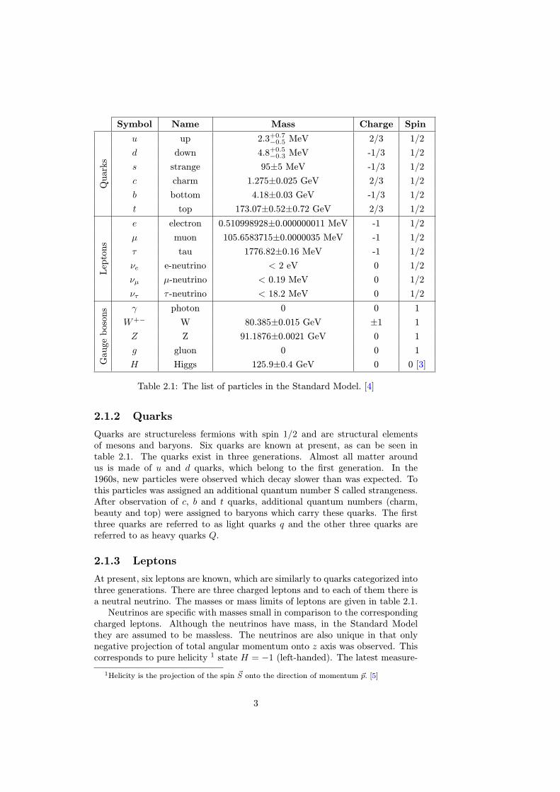
Particle physics is dealing with the particles that are the constituents of what isusually referred to as matter and radiation. There were many models trying todescribe well known phenomena and physical laws. In the 1970s, the StandardModel (SM) of particles and their interactions was formed. This model is inbest agreement with experimental data. The Standard Model assumes, that ourworld is made of 17 elementary particles. The first group is called fermions andhas a half-integer spin. The second group is called bosons and has an integerspin. The particles interact via four known types of forces: electromagnetic,strong, weak and gravitational which latter not being part of the SM. Thecomplete list of elementary particles and some of their properties is shown inTab. 2.1.

2.1.1 Fundamental interactions

Interactions in the Standard Model are realized as an exchange of mediatingbosons, characteristic to the type of interaction between its constituents. Dueto their character, they are frequently called exchange interactions.Electromagnetic interaction is mediated by a massless photon and it has

infinite range. This interaction acts between charged particles. The theorydescribing the electromagnetic interaction is called quantum electrodynamics(QED) and it later laid the ground of the quantum field theory (QFT), theframework for description of other interactions in the Standard Model.Strong interaction binds quarks together in hadrons and is mediated by the

exchange of massless gluons. Strong force is the strongest force compared toother forces, and its range is limited to 1 fm.Weak interaction is responsible for the relatively slow processes of β decay.

The mediators of this interaction are W± and Z0 bosons. It is characterised bylong lifetimes and small cross sections.Gravitational interaction acts between all particles. Gravitational force is

the weakest of all fundamental forces, and is almost 10−38 times weaker thanstrong interaction. Due to this fact, gravitational interaction is neglected in theSM. In the some particle theories, this interaction is mediated by a hypotheticalparticle graviton with spin 2.

2

Symbol Name Mass Charge Spin

Qua

rks

u up 2.3+0.7−0.5 MeV 2/3 1/2

d down 4.8+0.5−0.3 MeV -1/3 1/2

s strange 95±5 MeV -1/3 1/2

c charm 1.275±0.025 GeV 2/3 1/2

b bottom 4.18±0.03 GeV -1/3 1/2

t top 173.07±0.52±0.72 GeV 2/3 1/2

Lep

tons

e electron 0.510998928±0.000000011 MeV -1 1/2

µ muon 105.6583715±0.0000035 MeV -1 1/2

τ tau 1776.82±0.16 MeV -1 1/2

νe e-neutrino < 2 eV 0 1/2

νµ µ-neutrino < 0.19 MeV 0 1/2

ντ τ -neutrino < 18.2 MeV 0 1/2

Gau

geb

oson

s γ photon 0 0 1

W+− W 80.385±0.015 GeV ±1 1

Z Z 91.1876±0.0021 GeV 0 1

g gluon 0 0 1

H Higgs 125.9±0.4 GeV 0 0 [3]

Table 2.1: The list of particles in the Standard Model. [4]

2.1.2 Quarks

Quarks are structureless fermions with spin 1/2 and are structural elementsof mesons and baryons. Six quarks are known at present, as can be seen intable 2.1. The quarks exist in three generations. Almost all matter aroundus is made of u and d quarks, which belong to the first generation. In the1960s, new particles were observed which decay slower than was expected. Tothis particles was assigned an additional quantum number S called strangeness.After observation of c, b and t quarks, additional quantum numbers (charm,beauty and top) were assigned to baryons which carry these quarks. The firstthree quarks are referred to as light quarks q and the other three quarks arereferred to as heavy quarks Q.

2.1.3 Leptons

At present, six leptons are known, which are similarly to quarks categorized intothree generations. There are three charged leptons and to each of them there isa neutral neutrino. The masses or mass limits of leptons are given in table 2.1.

Neutrinos are specific with masses small in comparison to the correspondingcharged leptons. Although the neutrinos have mass, in the Standard Modelthey are assumed to be massless. The neutrinos are also unique in that onlynegative projection of total angular momentum onto z axis was observed. Thiscorresponds to pure helicity 1 state H = −1 (left-handed). The latest measure-

1Helicity is the projection of the spin ~S onto the direction of momentum ~p. [5]

3

ment of the Planck detector provides the upper limit for sum of the neutrinomasses mνi [6] ∑

i

mνi < 0.25 eV. (2.1)

2.1.4 Antiparticles

To every particle exists corresponding antiparticle with same mass and lifetimebut with opposite charge and magnetic moment.

The existence of antiparticles is a general property of both fermions andbosons. The first observed antiparticle was the antiparticle of an electron, whichis called positron. Due to the conservation laws, fermions must be created anddestroyed in pairs. This mechanism is called pair-production and annihilation.

2.2 Strong interaction

2.2.1 Colour

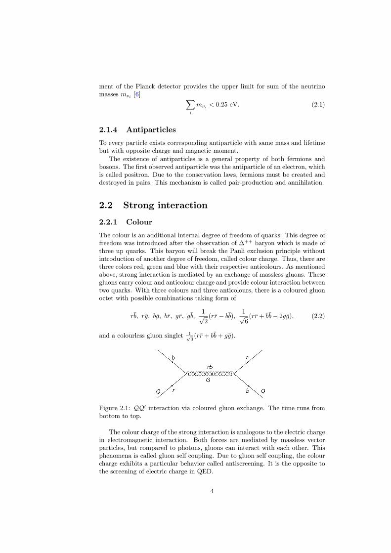
The colour is an additional internal degree of freedom of quarks. This degree offreedom was introduced after the observation of ∆++ baryon which is made ofthree up quarks. This baryon will break the Pauli exclusion principle withoutintroduction of another degree of freedom, called colour charge. Thus, there arethree colors red, green and blue with their respective anticolours. As mentionedabove, strong interaction is mediated by an exchange of massless gluons. Thesegluons carry colour and anticolour charge and provide colour interaction betweentwo quarks. With three colours and three anticolours, there is a coloured gluonoctet with possible combinations taking form of

rb, rg, bg, br, gr, gb,1√2

(rr − bb), 1√6

(rr + bb− 2gg), (2.2)

and a colourless gluon singlet 1√3(rr + bb+ gg).

Figure 2.1: QQ′ interaction via coloured gluon exchange. The time runs frombottom to top.

The colour charge of the strong interaction is analogous to the electric chargein electromagnetic interaction. Both forces are mediated by massless vectorparticles, but compared to photons, gluons can interact with each other. Thisphenomena is called gluon self coupling. Due to gluon self coupling, the colourcharge exhibits a particular behavior called antiscreening. It is the opposite tothe screening of electric charge in QED.

4

(a) (b)

Figure 2.2: Screening of electric charge by virtual electron-positron pairs in (a)and antiscreening of the colour charge by gluons and screening by quarks in(b). [7]

Both baryons and mesons must be colourless, thus the quarks and gluonsare confined inside hadrons. No free quarks were observed , with the exceptionof the top quark, which decays before it has a chance to hadronize.

2.2.2 QCD

The theory describing the interactions between quarks and gluons based on acolour exchange is called quantum chromodynamics (QCD). Despite photonsand gluons being massless, the QCD potential takes a different form due to thedifferences between those forces. The simplest potential model for mesons thatdescribes strong interaction is called Cornell potential model and it takes form

Vs(r) = −4

3

αsr

+ kr, (2.3)

where αs is the strong interaction coupling and k is a free parameter. The firstpart of the equation is similar to the Coulomb potential with a factor of 4

3 . Thisfactor arises from eight colour gluon states averaged over three quark colours.The factor is divided by 2 from the definition of αs. The second, linear term isassociated with colour confinement at large r.

The Cornell potential can be extended by inclusion of the spin interactionbetween quarks. These spin-dependent potentials are assumed to be dominatedby a one-gluon exchange and consist of spin-spin, tensor and spin-orbit terms.For a system of two quarks, the potential takes the following form [8]:

Vqq = −4

3

αsr

+σr+32παs9m2

q

δ(r)Sq ·Sq+1

m2q

[(2αsr3− b

2r

)L · S +

4αsr3

T

], (2.4)

where the L is an orbital momentum, Sq is a spin momentum of a particularquark, S = Sq + Sq and T is a tensor term.

These extended models give better results, but still they are not satisfactory.Thus, the new interquark potential models are being developed and tested.

5

2.2.3 Running coupling

Charge screening in the QED (screening) and QCD (antiscreening) leads to theconcept of a running coupling (the energy dependence of a strong coupling). Inthe QED, the coupling becomes large at (very) short distance and large energies,but its effect is small. In the QCD, the antiscreening effect causes the strongcoupling to become small at short distance (large momentum transfer). Thiscauses the quarks inside hadrons to behave more or less like free particles. Thisproperty of the strong interaction is called asymptotic freedom.

On the other hand, at the increasing distance, the coupling becomes so strongthat it is impossible to isolate a quark from a hadron. In addition, if the quarkpair receives more energy than is necessary for the production of a new quarkantiquark pair, then it is energetically favourable to produce a new quark pair.This mechanism is called colour confinement.

Using perturbative QCD (pQCD) calculations and experimental data, thecoupling constant of the QCD can be shown to have the following energy scale-dependence

αs(Q) =2π

β0 ln QΛQCD

, (2.5)

where β0 = 11 − 23nf , with nf being the number of the active quark flavor,

and ΛQCD is the QCD scale [4]. The value of ΛQCD = (0.339 ± 0.010) GeV isdetermined by experiments. This dependence is valid only for Q2 � 2Λ2, wherethe Q is transferred momentum. The summary of measurements of αs(Q) frommultiple experiments is shown in Figure 2.3.

Figure 2.3: Summary of measurements of αs(Q) as a function of the respectiveenergy scale Q. The respective degree of the QCD perturbation theory used inthe extraction of αs is indicated in brackets (NLO: next-to-leading order; NNLO:next-to-next-to leading order; res. NNLO: NNLO matched with resumed next-to-leading logs; N3LO: next-to-NNLO)2. [4]

2NLO etc. are the levels of the perturbation QCD theory into which the Feynman diagramsare counted.

6

2.3 Heavy quarkonia production

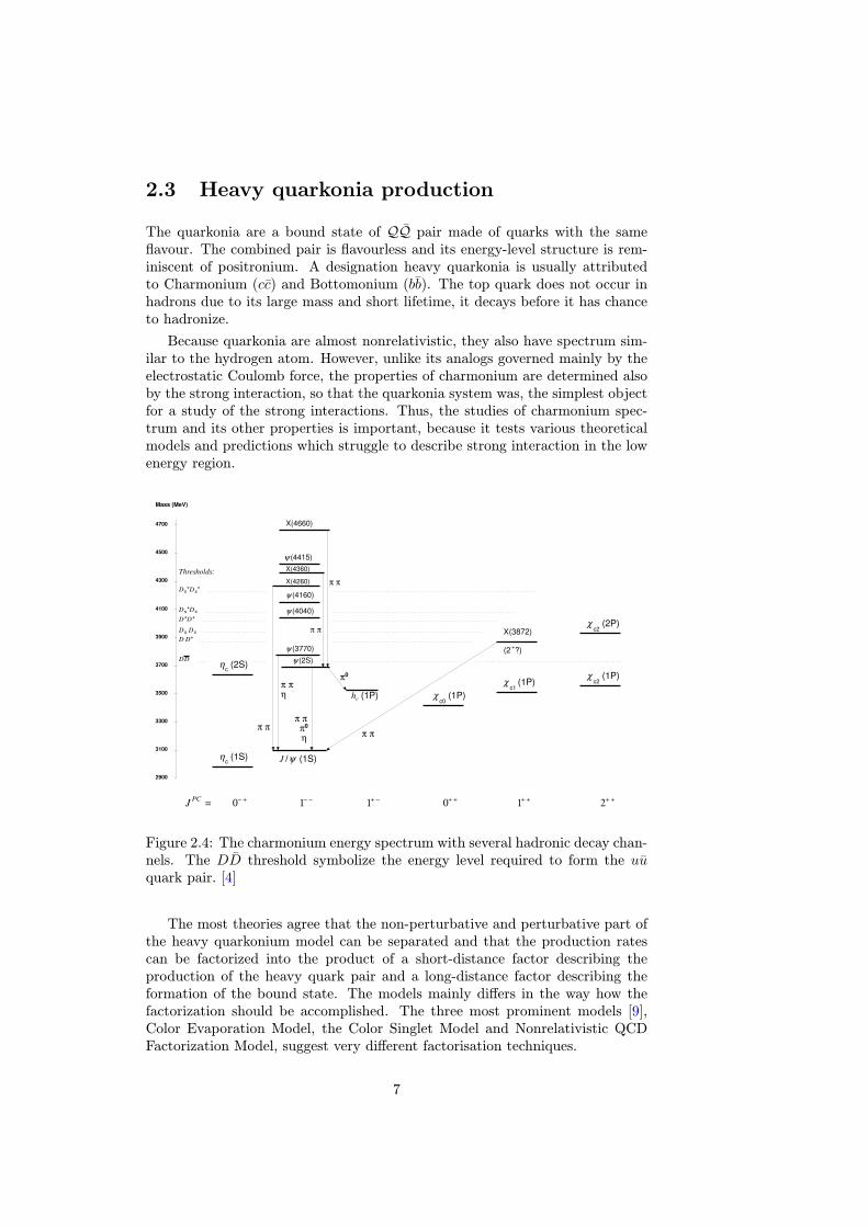
The quarkonia are a bound state of QQ pair made of quarks with the sameflavour. The combined pair is flavourless and its energy-level structure is rem-iniscent of positronium. A designation heavy quarkonia is usually attributedto Charmonium (cc) and Bottomonium (bb). The top quark does not occur inhadrons due to its large mass and short lifetime, it decays before it has chanceto hadronize.

Because quarkonia are almost nonrelativistic, they also have spectrum sim-ilar to the hydrogen atom. However, unlike its analogs governed mainly by theelectrostatic Coulomb force, the properties of charmonium are determined alsoby the strong interaction, so that the quarkonia system was, the simplest objectfor a study of the strong interactions. Thus, the studies of charmonium spec-trum and its other properties is important, because it tests various theoreticalmodels and predictions which struggle to describe strong interaction in the lowenergy region.

= PC

J− +0 − −1 + +0 + +1+ −1 + +2

(2S) c

η

(1S) c

η

(2S)ψ

(4660)X

(4360)X

(4260)X

(4415)ψ

(4160)ψ

(4040)ψ

(3770)ψ

(1S) ψ/J

(1P) c

h

(1P) c2

χ

(2P) c2

χ(3872)X

?)­+

(2

(1P) c1

χ

(1P) c0

χ

0π

π π

η

0π

π πη

π π

π π

π π

π π

Thresholds:

DD

*D D

sD sD

*D*D

sD*sD

*sD*sD

2900

3100

3300

3500

3700

3900

4100

4300

4500

4700

Mass (MeV)

Figure 2.4: The charmonium energy spectrum with several hadronic decay chan-nels. The DD threshold symbolize the energy level required to form the uuquark pair. [4]

The most theories agree that the non-perturbative and perturbative part ofthe heavy quarkonium model can be separated and that the production ratescan be factorized into the product of a short-distance factor describing theproduction of the heavy quark pair and a long-distance factor describing theformation of the bound state. The models mainly differs in the way how thefactorization should be accomplished. The three most prominent models [9],Color Evaporation Model, the Color Singlet Model and Nonrelativistic QCDFactorization Model, suggest very different factorisation techniques.

7

2.3.1 Color Singlet Model

In the Color Singlet Model (CSM), the perturbative and non-perturbative partsof the quarkonium production process are completly correlated. In this modelthe QQ pair is directly prepared with the proper quantum numbers in the initialhard subprocess, only then is non-zero probability to form the correspondingfinal state. The gluons can not adjust quantum numbers in this theory and theyonly serve to generate binding potential.

The CSM correctly predicts the normalization and momentum dependenceof the J/ψ photoproduction rate, but it fails to adequately reproduce otheravailable data on quarkonium production. Its predictions of the directly pro-duced J/ψ and ψ(2S) hadroproduction rates are smaller by more than an orderof magnitude.

2.3.2 Color Evaporation Model

In the Color Evaporation Model (CEM), the perturbative and non-perturbativeparts of the quarkonium production process are considered to be uncorrelated.The production cross section of all quarkonia states in CEM is some fraction ofthe overallQQ pairs cross section below the HH threshold where H is the lowestmass hadron with corresponding heavy quark. The CEM cross section is thensimply theQQ production cross section with a cut on the pair mass. In the CEMthere are not any constrains on the color or spin of the final state, because theproduced QQ pair neutralizes its color by interaction with the collision-inducedcolor field, thus the name ”color evaporation”. The interaction with color fieldcan be described by the multiple soft gluon emissions. The soft interactionsassumed to be universal and the effect on the dynamics of the quarkonium stateis negligible.

The CEM predicts zero polarization of the J/ψ which is valid only for thelow pT regions.

2.3.3 Nonrelativistic QCD Factorization Model

The Nonrelativistic QCD Factorization Model based on the effective field theoryNonrelativistic QCD (NRQCD) and lies somewhere between the previous twomodels. It predicts non-zero probability for any quark pair to produce almostany quarkonium state but the probability depends on the initial quantum state.

The quarkonium production cross section, in the NRQCD factorization model,can be written as

σ(H) =∑n

Fn(Λ)

mdn−4Q

〈0|OHn |0〉, (2.6)

where H is the quarkonium state Λ is the ultraviolet cutoff of the effective theory,the Fn are short-distance coefficients, and the OHn are four-fermion operators,whose mass dimensions are dn .

The short-distance coefficients Fn(Λ) are essentially the process-dependentpartonic cross sections to make a QQ pair. The QQ pair can be produced in acolor-singlet state or in a color-octet state. The short-distance coefficients aredetermined by matching the square of the production amplitude in NRQCDto full QCD. Because the QQ production scale is of order mQ or greater, thismatching can be carried out in perturbation theory.

8

The Nonrelativistic QCD Factorization Model successfully reproduced vari-ous quarkonia data and fits well on the experiment, but there are areas where arestill some problems. Recently the proof of the factorisation in heavy quarkoniumproduction in NRQCD Factorization Model was introduced at next-to-next-to-leading order (NNLO) in coupling constant by using diagrammatic method ofQCD [10].

2.4 kt-factorization approach [1]

This method how to do the factorization is based on another way how to describethe structure function, when incident gluons have non-zero transverse momentain small-x region. This non-zero transverse momenta is result of the diffusionof parton evolution.

The exact expression for kt gluon distribution can be obtained as a solutionof the evolution equation which, contrary to the parton model case, is nonlineardue to interactions between the partons in small x region.

The biggest advantage compared to the classical parton model is that themain part of the NLO and even NNLO corrections are effectively included inthe kt-factorization approach, due to the off-shell gluons.

9

Chapter 3

The ATLAS detector [2]

The ATLAS (A Toroidal LHC ApparatuS) detector is general-purpose detectordesigned to study p-p collisions at the LHC (Large Hadron Collider) locatedin the CERN laboratory near Geneva, Switzerland. The LHC is designed toprovide proton beams with

√s = 14 TeV with a design luminosity 1034 cm−2 s−1

and reaction rate of 40 MHz. However during first run period, the LHC wasoperating at lower energy of

√s = 7 TeV in 2011 and

√s = 8 TeV in 2012. The

reaction of 20 MHz rate is also lower than designed one. The LHC also providescollisions of Pb208 ions with energy

√s = 5.5 TeV per nucleon pair, at designed

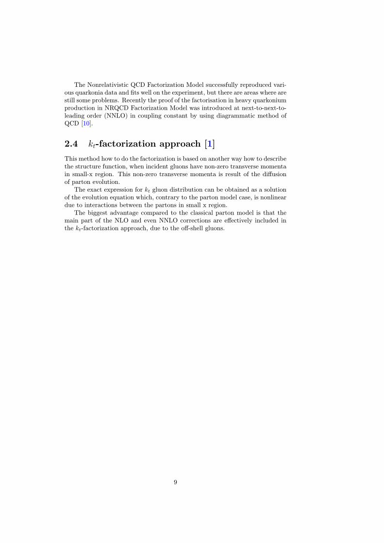
luminosity of 1027 cm−2 s−1.The ATLAS cover almost the full solid angle around the collision point and

is symmetric in the forward-backward direction with respect to the interactionpoint. It can be divided into barrel section, end-caps and forward region. Thesubdetectors can be divided into three sections inner detector (ID), calorimetrysystems and muon spectrometer (MS).

Figure 3.1: ATLAS detector cut-away view with its subdetectors highlighted. [2]

10

3.1 Inner detector

The inner detector is designed to provide an excellent momentum resolution forcharged particles and both primary and secondary vertex position measurementswith high precision in the pseudorapidity range of |η| < 2.5. The ID haveto withstand high-radiation environment as the innermost subsystem of theATLAS detector.

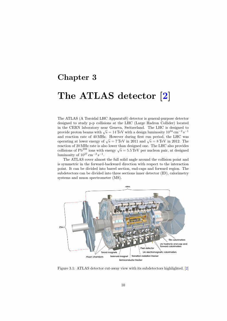
The ID is contained within a cylindrical envelope of a length of ±3512 mmand of a radius of 1150 mm, and is immersed in a 2 T magnetic field generated bythe central superconducting solenoid. The ID consists of a silicon pixel detector,a silicon strip detector (SCT) and a transition radiation tracker (TRT).

As can be seen in figure , the detectors are arranged as concentric cylindersaround the beam axis in the barrel region. In the end-cap regions, there arepixel modules located on disks perpendicular to the beam axis. All detectorsare mounted on a support structure, which is made of carbon fibers to ensuregood mechanical properties, thermal conduction and low material budget.

Figure 3.2: The schematic cut-away view of ATLAS inner detector. [2]

3.1.1 Pixel detector

The pixel detector contains three layers of the pixel modules in the barrel region(called ID layers 0–2) and two end-caps, each with three disk layers. The 0th

layer is also referred to as B-layer. The layers are equipped by silicon pixeldetectors with nominal pixel size of 50× 400 µm2 . The sensor thickness isapproximately 250 µm. Silicon pixel sensors use planar technology with oxy-genated n-type wafers and are read out on the n+ -implanted side of the sensor.The opposite side of the electrodes is in contact with a p+ layer. Each pixelsensor is bump-bonded through hole in the sensor passivation layer to front-endreadout electronic chip. The pixel detector provides approximately 80.4 millionreadout channels in total.

11

During first long shutdown between years 2013 and 2015, upgrades are beingmade. The fourth layer of the pixel detector is added. This layer is placedbetween beampipe and current b-layer and is called the Insertable B-layer (IBL).This IBL is be equipped with new sensors using planar n-in-n and 3D double-sided n-in-p technology. These sensors have finer granularity of 50× 250 µm2andbesides higher radiation tolerance, new readout chip FE-I4 has lower noise andpower consumption.

3.1.2 SCT detector

SCT detector consist of four layers of double detectors in the barrel region (calledID layers 3–6) and two end-cap regions, each containing nine layers. Layersare equipped by modules which consist of 80 µm pitch micro-strip sensors withthickness 285± 15 µm, providing R− Φ coordinates.

Every two sensor modules are glued together in the barrel region within ahybrid module. On one detector layer, there are 2 sensor layers rotated withintheir hybrids by ±20 mrad around the geometrical center of the sensor to mea-sure both R− Φ× z coordinates.

For reason of cost and reliability, the sensors of SCT use classic single-sidedp-in-n technology. The sensors are connected to a binary signal readout chips.In total, the SCT provides approximately 6.3 million readout channels.

3.1.3 Transition radiation tracker

Main purpose of TRT is to measure transition radiation of charged particles, inorder to distinguish between light electrons and other particles, in the pseudo-rapidity range of |η| < 2.0. The TRT consist of 73 layers of straws in the barrelregion and 160 straw planes in end-cap. Typically, the TRT gives 36 hits pertrack, but it provides only R− Φ information.

The basic TRT detector elements are polyamide drift straw tubes with diam-eter of 4 mm filled by special gaseous mixture. The straw tube walls operates ascathodes, while the 31 µm thick tungsten wire plated with 0.5 µm–0.7 µm layerof gold operates as anode. The total number of readout channels of TRT isapproximately 351,000.

3.2 Calorimetry

Calorimetry system is designed to provide good energy resolution for measure-ment of electromagnetic and hadronic showers, and it must also limit punch-through into the muon system. Calorimetry system consist of two separatecalorimeters using different designs suited to the widely varying requirements ofthe physics processes of interest, and it cover region up to |η| < 4.9. Over the ηregion matched to the inner detector, the fine granularity of the EM calorimeteris ideally suited for measurements of electrons and photons. There is coarsergranularity in the rest of the detector, but calorimeters are precise enough tosatisfy the physics requirements for jet reconstruction and Emiss

T measurement.

12

3.3 Muon spectrometer

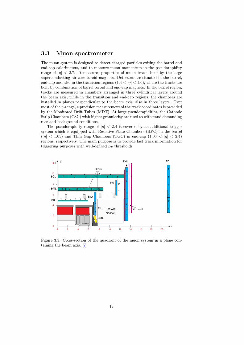
The muon system is designed to detect charged particles exiting the barrel andend-cap calorimeters, and to measure muon momentum in the pseudorapidityrange of |η| < 2.7. It measures properties of muon tracks bent by the largesuperconducting air-core toroid magnets. Detectors are situated in the barrel,end-cap and also in the transition regions (1.4 < |η| < 1.6), where the tracks arebent by combination of barrel toroid and end-cap magnets. In the barrel region,tracks are measured in chambers arranged in three cylindrical layers aroundthe beam axis, while in the transition and end-cap regions, the chambers areinstalled in planes perpendicular to the beam axis, also in three layers. Overmost of the η-range, a precision measurement of the track coordinates is providedby the Monitored Drift Tubes (MDT). At large pseudorapidities, the CathodeStrip Chambers (CSC) with higher granularity are used to withstand demandingrate and background conditions.

The pseudorapidity range of |η| < 2.4 is covered by an additional triggersystem which is equipped with Resistive Plate Chambers (RPC) in the barrel(|η| < 1.05) and Thin Gap Chambers (TGC) in end-cap (1.05 < |η| < 2.4)regions, respectively. The main purpose is to provide fast track information fortriggering purposes with well-defined pT thresholds.

Figure 3.3: Cross-section of the quadrant of the muon system in a plane con-taining the beam axis. [2]

13

Chapter 4

Data analysis

4.1 Data acquisition and processing

The data were taken during LHC run1 in proton-proton collisions at both 7 TeVand 8 TeV where only the data collected with a stable beam operation are used.The criteria of quality were applied at the luminosity block levels, where theluminosity block, which lasts 60 seconds, is an atomic unit of the ATLAS data.To ensure the quality criteria the collected data are filtered by a Good Runs List(GRL), which take in account the prescale levels and triggers dead time. Theintegrated luminosity of both samples after trigger pass are 2.2 fb−1 for 2011data and 11.45 fb−1 for 2012 data.

4.2 Event reconstruction

To measure the J/ψ and ψ′ production cross section the di-muon channel waschosen, because the muons have clean detector signature. To reconstruct muontracks, several different strategies have been developed using physics signaturesin the inner detector, calorimeters and muon detector system. Muons can beclassified into four categories according to the signatures left in the detector:

• Standalone muons are identified using only Muon Spectrometer. Thetracks are extrapolated to the beam region to give the track parameters.Due to the position and momentum resolution of the muon chambers, theirparameters are not measured as precisely as in other muon reconstructiontypes, but provide muons from higher psoudorapidity |η| < 2.7.

• Combined muons are formed by matching the Inner Detector track to theMuon Spectrometer track. Two algorithms, Staco and Muid, are usedto identify the combined muons. They have the most precisely measuredparameters.

• Tagged muons are the ID tracks matched to the hits in the muon segmentsin the Muon Spectrometer. There are two tagging algorithms, MuTag andMuGirl, propagating all inner detector tracks with a sufficient momentumout to the first station of the muon spectrometer and search for nearbysegments.

14

• Calorimeter tagged muons use information about energy deposit in thecalorimetry system matched to the ID tracks. The calorimeter muonshave lower purity and efficiency than the muons reconstructed in the muonsystem.

To reconstruct di-muon candidates only combined muons are used to guar-antee the purity of the signal. In 2011, two algorithms called the STACO (Sta-tistical combination of the inner and outer track vectors) and Muid (a partialrefit using the original hits in both ID and MS) are used to reconstruct dimuoncandidates. Each of these algorithm produces its own chain called STACO andMuid. The STACO chain is used in this analysis for 2011 data, but the resultshould not be affected by this choice. Because both of these chains demon-strated their excellent capabilities of supporting physics analyses with muons,in 2012 they have been merged into a third, unified chain called Muons.

4.3 Event selection

The J/ψ and ψ(2S) candidates triggered by the trigger, which required twooppositely charged muons with pT > 4 GeV, have to pass multiple selectioncriteria. At first reconstructed candidate must fit within |η| < 2.3 and invari-ant mass window of 2.6 GeV–4.0 GeV. Both offline reconstructed muons arerestricted to pT > 4 GeV and |η| < 2.5. To ensure high purity of the signaleach track is required to have at least one Pixel hit, five SCT hits and in casethe track is within 0.1 < |η| < 1.9 at least six TRT hits. The maximum of themissing hits is in the Pixel and SCT layers is 2. For TRT hits is additionalcondition to have at least 90% of hits over outliners. The muon candidatesmust to be matched within a cone ∆R =

√(∆η)2 + (∆Φ)2 < 0.01 between

each reconstructed muon candidate and the trigger identified candidates. Thislast constraint reject about 5% of candidates but ensures, that the trigger wasfired by a measured muon and so the trigger unfolding can be performed.

4.4 Analysis prerequisites

The measurement is performed in several intervals of dimuon transverse mo-mentum and absolute value of rapidity. The dimuon pT range is restricted bykinematics conditions of pT (µµ) > 8 GeV. The condition of sufficient statisticssets upper limit to pT < 100 GeV.

The measurement differs two compounds of signal prompt and non-prompt,for both J/ψ or ψ(2S) (hereafter called ψ(nS)). The definition of promptrefers to the ψ(nS) states produced from short-lived QCD sources, this includesdirectly produced ψ(nS) in pp collision or indirectly produced ψ(nS) from feed-down from other charmonium states. If the decay chain includes long-livedparticles such as b-hadrons then the ψ(nS) is labeled as non-prompt.

15

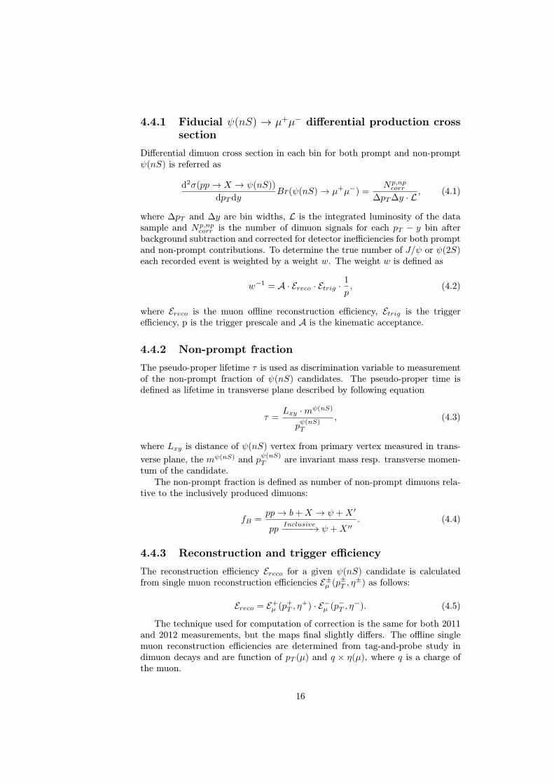
4.4.1 Fiducial ψ(nS) → µ+µ− differential production crosssection

Differential dimuon cross section in each bin for both prompt and non-promptψ(nS) is referred as

d2σ(pp→ X → ψ(nS))

dpTdyBr(ψ(nS)→ µ+µ−) =

Np,npcorr

∆pT∆y · L, (4.1)

where ∆pT and ∆y are bin widths, L is the integrated luminosity of the datasample and Np,np

corr is the number of dimuon signals for each pT − y bin afterbackground subtraction and corrected for detector inefficiencies for both promptand non-prompt contributions. To determine the true number of J/ψ or ψ(2S)each recorded event is weighted by a weight w. The weight w is defined as

w−1 = A · Ereco · Etrig ·1

p, (4.2)

where Ereco is the muon offline reconstruction efficiency, Etrig is the triggerefficiency, p is the trigger prescale and A is the kinematic acceptance.

4.4.2 Non-prompt fraction

The pseudo-proper lifetime τ is used as discrimination variable to measurementof the non-prompt fraction of ψ(nS) candidates. The pseudo-proper time isdefined as lifetime in transverse plane described by following equation

τ =Lxy ·mψ(nS)

pψ(nS)T

, (4.3)

where Lxy is distance of ψ(nS) vertex from primary vertex measured in trans-

verse plane, the mψ(nS) and pψ(nS)T are invariant mass resp. transverse momen-

tum of the candidate.The non-prompt fraction is defined as number of non-prompt dimuons rela-

tive to the inclusively produced dimuons:

fB =pp→ b+X → ψ +X ′

ppInclusive−−−−−−→ ψ +X ′′

. (4.4)

4.4.3 Reconstruction and trigger efficiency

The reconstruction efficiency Ereco for a given ψ(nS) candidate is calculatedfrom single muon reconstruction efficiencies E±µ (p±T , η

±) as follows:

Ereco = E+µ (p+

T , η+) · E−µ (p−T , η

−). (4.5)

The technique used for computation of correction is the same for both 2011and 2012 measurements, but the maps final slightly differs. The offline singlemuon reconstruction efficiencies are determined from tag-and-probe study indimuon decays and are function of pT (µ) and q × η(µ), where q is a charge ofthe muon.

16

(a) (b)

Figure 4.1: The reconstruction efficiency maps for both 7 TeV and 8 TeV dataas a function of the muon charge-signed pseudorapidity and muon pT .

Similar to reconstruction efficiency, the trigger efficiency Etrig for givenψ(nS) are calculated from single muon efficiencies E±RoI(p

±T , q, η

±). The ad-ditional correction factor cµµ(∆R, |yµµ|) must be used to include dimuon effectssuch as overlapping RoIs or vertex quality. The trigger efficiency is then com-puted as

Etrig = E+RoI(p

+T , q, η

+) · E−RoI(p−T , q, η

−) · cµµ(∆R, |yµµ|). (4.6)

This correction factor, computed from tag-and-probe, is divided in threebins of rapidity. Because the efficiency maps calculated directly from 2012 datahave issue with low pT and high rapidity events additional MC correction aveto be applied. This is made by fraction of two additional maps for low pT tagmuons, which are not available from data, and high pT EF mu18 trigger as wellfrom MC simulation. The efficiencies were provided by the ATLAS B-physicsgroup and are preliminary.

In 2012 data were observed an issue, where the 4% of events which fired the”EF 2mu4T Jpsimumu L2StarB” trigger have not stored its trigger objects.Unfortunately, these events are correlated and thus should not be omitted fromthe analysis. To handle this out additional systematics should be applied.

4.4.4 Acceptance

The kinematic acceptanceA(pT , y) is the probability that the muons from ψ(nS)with rapidity y and transverse momentum pT fall into fiducial volume of theATLAS detector. The acceptance maps are computed using Monte Carlo gen-erator applying selection criteria on particle momenta and rapidity to emulatethe detector geometry.

The acceptance also depend on spin alignment of ψ(nS) production mecha-nism, which is not well known for LHC conditions. This affects angular distri-bution of dimuon decays. The general decay frame of ψ(nS) candidate is givenby

d2N

d cos θ?dφ?∝ 1 + λθ cos2 θ? + λφ sin2 θ? cos 2φ? + λθφ sin 2θ? cosφ?, (4.7)

17

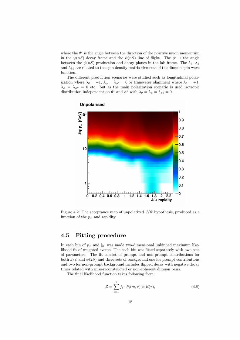
where the θ? is the angle between the direction of the positive muon momentumin the ψ(nS) decay frame and the ψ(nS) line of flight. The φ? is the anglebetween the ψ(nS) production and decay planes in the lab frame. The λθ, λφand λθφ are related to the spin density matrix elements of the dimuon spin wavefunction.

The different production scenarios were studied such as longitudinal polar-ization where λθ = −1, λφ = λφθ = 0 or transverse alignment where λθ = +1,λφ = λφθ = 0 etc., but as the main polarization scenario is used isotropicdistribution independent on θ? and φ? with λθ = λφ = λφθ = 0.

Figure 4.2: The acceptance map of unpolarized J/Ψ hypothesis, produced as afunction of the pT and rapidity.

4.5 Fitting procedure

In each bin of pT and |y| was made two-dimensional unbinned maximum like-lihood fit of weighted events. The each bin was fitted separately with own setsof parameters. The fit consist of prompt and non-prompt contributions forboth J/ψ and ψ(2S) and three sets of background one for prompt contributionsand two for non-prompt background includes flipped decay with negative decaytimes related with miss-reconstructed or non-coherent dimuon pairs.

The final likelihood function takes following form:

L =

7∑i=1

fi · Pi(m, τ)⊗R(τ), (4.8)

18

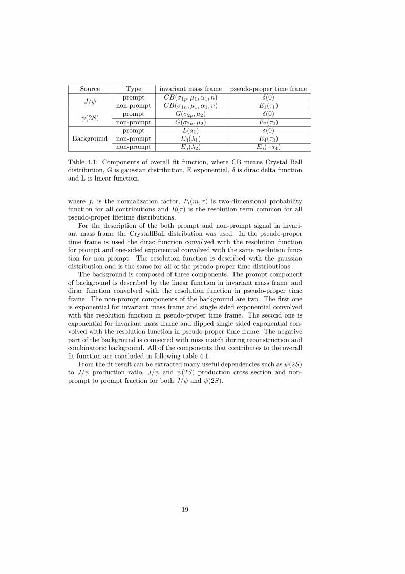
Source Type invariant mass frame pseudo-proper time frame

J/ψprompt CB(σ1p, µ1, α1, n) δ(0)

non-prompt CB(σ1n, µ1, α1, n) E1(τ1)

ψ(2S)prompt G(σ2p, µ2) δ(0)

non-prompt G(σ2n, µ2) E2(τ2)

Backgroundprompt L(a1) δ(0)

non-prompt E3(λ1) E4(τ3)non-prompt E5(λ2) E6(−τ4)

Table 4.1: Components of overall fit function, where CB means Crystal Balldistribution, G is gaussian distribution, E exponential, δ is dirac delta functionand L is linear function.

where fi is the normalization factor, Pi(m, τ) is two-dimensional probabilityfunction for all contributions and R(τ) is the resolution term common for allpseudo-proper lifetime distributions.

For the description of the both prompt and non-prompt signal in invari-ant mass frame the CrystallBall distribution was used. In the pseudo-propertime frame is used the dirac function convolved with the resolution functionfor prompt and one-sided exponential convolved with the same resolution func-tion for non-prompt. The resolution function is described with the gaussiandistribution and is the same for all of the pseudo-proper time distributions.

The background is composed of three components. The prompt componentof background is described by the linear function in invariant mass frame anddirac function convolved with the resolution function in pseudo-proper timeframe. The non-prompt components of the background are two. The first oneis exponential for invariant mass frame and single sided exponential convolvedwith the resolution function in pseudo-proper time frame. The second one isexponential for invariant mass frame and flipped single sided exponential con-volved with the resolution function in pseudo-proper time frame. The negativepart of the background is connected with miss match during reconstruction andcombinatoric background. All of the components that contributes to the overallfit function are concluded in following table 4.1.

From the fit result can be extracted many useful dependencies such as ψ(2S)to J/ψ production ratio, J/ψ and ψ(2S) production cross section and non-prompt to prompt fraction for both J/ψ and ψ(2S).

19

[MeV]ψJ/

m2600 2800 3000 3200 3400 3600 3800 4000

Events

/ (

14 )

1

10

210

310

410

pseudo­proper time [ps]

­4 ­2 0 2 4 6 8 10E

vents

/ (

0.1

4 )

1

10

210

310

410

Figure 4.3: The projection of simultaneous fit result for 18 GeV < pT < 20 GeVand 0.75 < |y| < 1.00 bin in 7 TeV data. The invariant mass projection ispresented on the left side and the pseudo-proper time projection on the rightside.

[MeV]ψJ/

m2600 2800 3000 3200 3400 3600 3800 4000

Events

/ (

14 )

1

10

210

310

410

pseudo­proper time [ps]

­4 ­2 0 2 4 6 8 10

Events

/ (

0.1

4 )

1

10

210

310

410

510

Figure 4.4: The projection of simultaneous fit result for 18 GeV < pT < 20 GeVand 0.75 < |y| < 1.00 bin in 8 TeV data. The invariant mass projection ispresented on the left side and the pseudo-proper time projection on the rightside.

20

Chapter 5

Results

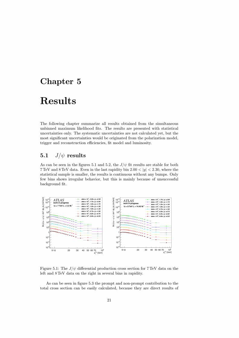
The following chapter summarize all results obtained from the simultaneousunbinned maximum likelihood fits. The results are presented with statisticaluncertainties only. The systematic uncertainties are not calculated yet, but themost significant uncertainties would be originated from the polarization model,trigger and reconstruction efficiencies, fit model and luminosity.

5.1 J/ψ results

As can be seen in the figures 5.1 and 5.2, the J/ψ fit results are stable for both7 TeV and 8 TeV data. Even in the last rapidity bin 2.00 < |y| < 2.30, where thestatistical sample is smaller, the results is continuous without any bumps. Onlyfew bins shows irregular behavior, but this is mainly because of unsuccessfulbackground fit.

[GeV]ψJ/

Tp

9 10 20 30 40 50 60 70 210

dy [nb/G

eV

]T

/ dp

2σ

) d

­µ

+µ

→ψ

Br(

J/

­610

­410

­210

1

210

410

610

810

1010

1210

1310

, 2.00< |y| <2.307data x 10

, 1.75< |y| <2.006

data x 10

, 1.50< |y| <1.755

data x 10

, 1.25< |y| <1.504data x 10

, 1.00< |y| <1.253

data x 10

, 0.75< |y| <1.002data x 10

, 0.25< |y| <0.751data x 10

, 0.00< |y| <0.250

data x 10

work in progressATLAS

­1 = 7 TeV L = 2.2 fbs

[GeV]ψJ/

Tp

9 10 20 30 40 50 60 70 210

dy [nb/G

eV

]T

/ dp

2σ

) d

­µ

+µ

→ψ

Br(

J/

­610

­410

­210

1

210

410

610

810

1010

1210

1310

, 1.75< |y| <2.007data x 10

, 1.50< |y| <1.756

data x 10

, 1.25< |y| <1.505

data x 10

, 1.00< |y| <1.254data x 10

, 0.75< |y| <1.003

data x 10

, 0.50< |y| <0.752data x 10

, 0.25< |y| <0.501data x 10

, 0.00< |y| <0.250

data x 10

work in progressATLAS

­1 = 8 TeV L = 14.45 fbs

Figure 5.1: The J/ψ differential production cross section for 7 TeV data on theleft and 8 TeV data on the right in several bins in rapidity.

As can be seen in figure 5.3 the prompt and non-prompt contribution to thetotal cross section can be easily calculated, because they are direct results of

21

[GeV]ψJ/

Tp

9 10 20 30 40 50 60 70 210

ψN

on­P

rom

pt F

raction J

/

­210

­110

1

10

210

310

410

510

610

710

810

910

1010

1110

1210

1310

, 2.00< |y| <2.307data x 10

, 1.75< |y| <2.006

data x 10

, 1.50< |y| <1.755

data x 10

, 1.25< |y| <1.504data x 10

, 1.00< |y| <1.253

data x 10

, 0.75< |y| <1.002data x 10

, 0.25< |y| <0.751data x 10

, 0.00< |y| <0.250

data x 10

work in progressATLAS

­1 = 7 TeV L = 2.2 fbs

[GeV]ψJ/

Tp

9 10 20 30 40 50 60 70 210

ψN

on­P

rom

pt F

raction J

/

­210

­110

1

10

210

310

410

510

610

710

810

910

1010

1110

1210

1310

, 1.75< |y| <2.007data x 10

, 1.50< |y| <1.756

data x 10

, 1.25< |y| <1.505

data x 10

, 1.00< |y| <1.254data x 10

, 0.75< |y| <1.003

data x 10

, 0.50< |y| <0.752data x 10

, 0.25< |y| <0.501data x 10

, 0.00< |y| <0.250

data x 10

work in progressATLAS

­1 = 8 TeV L = 14.45 fbs

Figure 5.2: The non-prompt J/ψ production fraction for 7 TeV data on the leftand 8 TeV data on the right in several bins in rapidity.

the fit. This can be done for ψ(2S) as well as J/ψ.

[GeV]T

p9 10 20 30 40 50 60 70 80 90 210

dy [nb/G

eV

]T

/ dp

2σ

) d

­µ

+µ

→ψ

Br(

J/

­410

­310

­210

­110

1

inclusive

prompt

non­prompt

Figure 5.3: The prompt and non-prompt contributions to the total cross sectionin 0.75 < |y| < 1.00 rapidity bin.

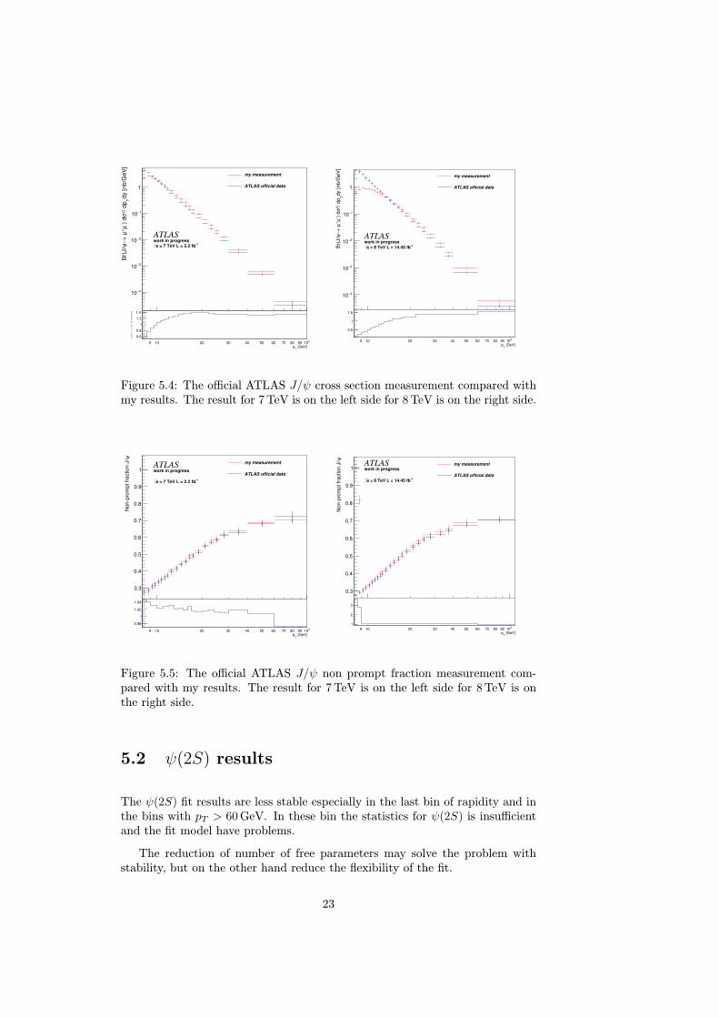
The figure 5.4 shows comparison of my measurement with official ATLASanalysis [11], where the my results shows some systematics shift. My measuredcross section are larger in the high pT but in the low pT are there is a rapiddecrease. On the other hand the non-prompt fraction of J/ψ is in agreementwith official ATLAS analysis without any irregularities. The reason of thisdisagreement are not yet known.

22

dy [nb/G

eV

]T

/ dp

2σ

) d

­µ

+µ

→ψ

Br(

J/

4−10

3−10

2−10

1−10

1

my measurement

ATLAS official data

work in progressATLAS

­1 = 7 TeV L = 2.2 fbs

[GeV]T

p9 10 20 30 40 50 60 70 80 90

210

dy [

nb

/GeV

]T

/ dp

2σ

) d

­µ

+µ

→ψ

Br(

J/

0.6

0.8

1

1.2

1.4

dy [nb/G

eV

]T

/ dp

2σ

) d

­µ

+µ

→ψ

Br(

J/

4−10

3−10

2−10

1−10

1

my measurement

ATLAS official data

work in progressATLAS

­1 = 8 TeV L = 14.45 fbs

[GeV]T

p9 10 20 30 40 50 60 70 80 90

210

0.5

1

1.5

Figure 5.4: The official ATLAS J/ψ cross section measurement compared withmy results. The result for 7 TeV is on the left side for 8 TeV is on the right side.

ψN

on­p

rom

pt fr

action J

/

0.3

0.4

0.5

0.6

0.7

0.8

0.9

1

my measurement

ATLAS official datawork in progressATLAS

­1 = 7 TeV L = 2.2 fbs

[GeV]T

p9 10 20 30 40 50 60 70 80 90

210

0.98

1

1.02

1.04

ψN

on­p

rom

pt fr

action J

/

0.3

0.4

0.5

0.6

0.7

0.8

0.9

1my measurement

ATLAS official data

work in progressATLAS

­1 = 8 TeV L = 14.45 fbs

[GeV]T

p9 10 20 30 40 50 60 70 80 90

210

1

2

3

Figure 5.5: The official ATLAS J/ψ non prompt fraction measurement com-pared with my results. The result for 7 TeV is on the left side for 8 TeV is onthe right side.

5.2 ψ(2S) results

The ψ(2S) fit results are less stable especially in the last bin of rapidity and inthe bins with pT > 60 GeV. In these bin the statistics for ψ(2S) is insufficientand the fit model have problems.

The reduction of number of free parameters may solve the problem withstability, but on the other hand reduce the flexibility of the fit.

23

[GeV]ψJ/

Tp

9 10 20 30 40 50 60 70 210

dy [nb/G

eV

]T

/ dp

2σ

) d

­µ

+µ

→ (

2S

)ψ

Br(

­810

­610

­410

­210

1

210

410

610

810

1010

1210

, 2.00< |y| <2.307data x 10

, 1.75< |y| <2.006

data x 10

, 1.50< |y| <1.755

data x 10

, 1.25< |y| <1.504data x 10

, 1.00< |y| <1.253

data x 10

, 0.75< |y| <1.002data x 10

, 0.25< |y| <0.751data x 10

, 0.00< |y| <0.250

data x 10

work in progressATLAS

­1 = 7 TeV L = 2.2 fbs

[GeV]ψJ/

Tp

9 10 20 30 40 50 60 70 210

dy [nb/G

eV

]T

/ dp

2σ

) d

­µ

+µ

→ (

2S

)ψ

Br(

­710

­510

­310

­110

10

310

510

710

910

1110

1210

, 1.75< |y| <2.007data x 10

, 1.50< |y| <1.756

data x 10

, 1.25< |y| <1.505

data x 10

, 1.00< |y| <1.254data x 10

, 0.75< |y| <1.003

data x 10

, 0.50< |y| <0.752data x 10

, 0.25< |y| <0.501data x 10

, 0.00< |y| <0.250

data x 10

work in progressATLAS

­1 = 8 TeV L = 14.45 fbs

Figure 5.6: The ψ(2S) differential production cross section for 7 TeV data onthe left and 8 TeV data on the right in several bins in rapidity.

[GeV]ψJ/

Tp

9 10 20 30 40 50 60 70 210

(2S

)ψ

Non­P

rom

pt F

raction

­210

­110

1

10

210

310

410

510

610

710

810

910

1010

1110

1210

1310

, 2.00< |y| <2.307data x 10

, 1.75< |y| <2.006

data x 10

, 1.50< |y| <1.755

data x 10

, 1.25< |y| <1.504data x 10

, 1.00< |y| <1.253

data x 10

, 0.75< |y| <1.002data x 10

, 0.25< |y| <0.751data x 10

, 0.00< |y| <0.250

data x 10

work in progressATLAS

­1 = 7 TeV L = 2.2 fbs

[GeV]ψJ/

Tp

9 10 20 30 40 50 60 70 210

(2S

)ψ

Non­P

rom

pt F

raction

­310

­210

­110

1

10

210

310

410

510

610

710

810

910

1010

1110

1210

1310

, 1.75< |y| <2.007data x 10

, 1.50< |y| <1.756

data x 10

, 1.25< |y| <1.505

data x 10

, 1.00< |y| <1.254data x 10

, 0.75< |y| <1.003

data x 10

, 0.50< |y| <0.752data x 10

, 0.25< |y| <0.501data x 10

, 0.00< |y| <0.250

data x 10

work in progressATLAS

­1 = 8 TeV L = 14.45 fbs

Figure 5.7: The non-prompt ψ(2S) production fraction for 7 TeV data on theleft and 8 TeV data on the right in several bins in rapidity.

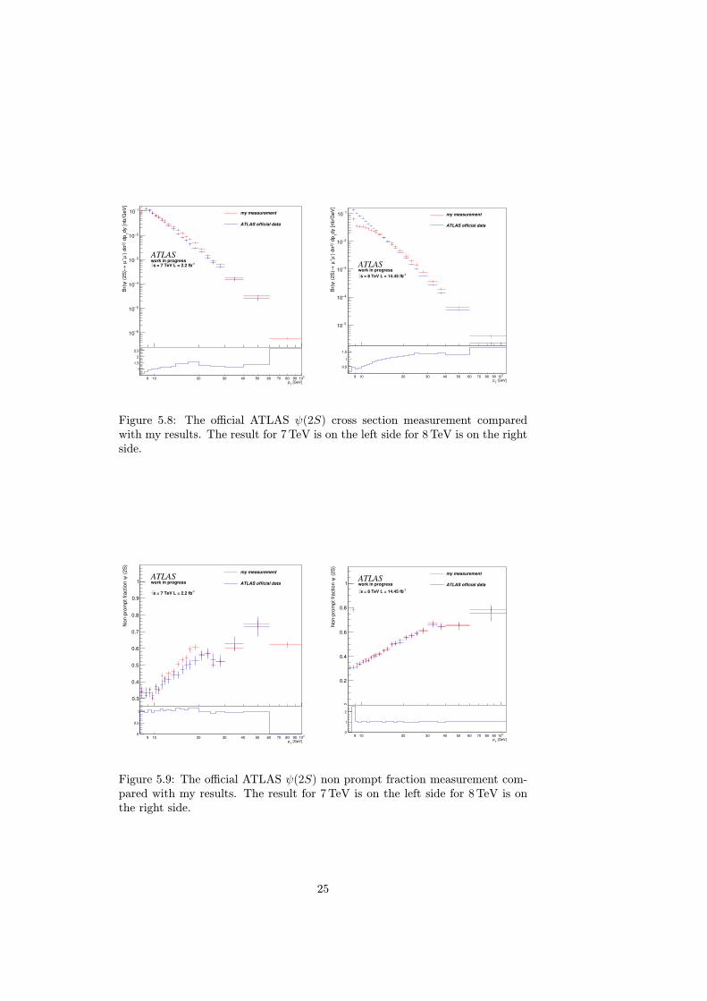
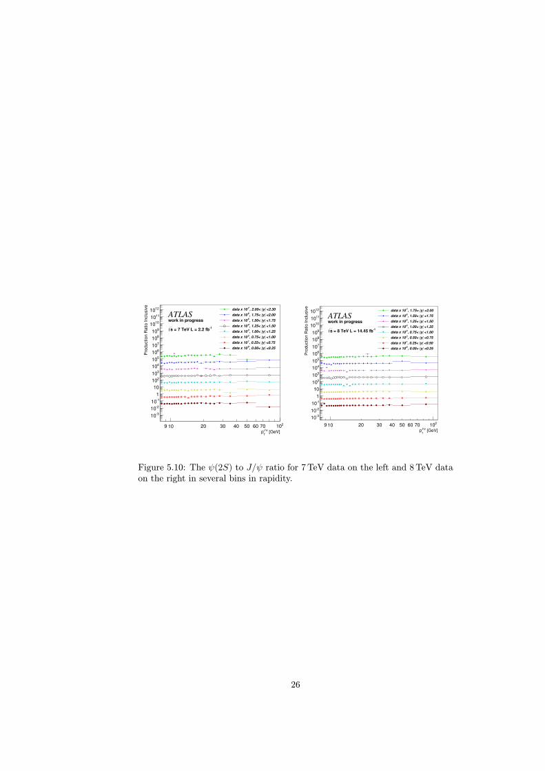
5.3 ψ(2S) to J/ψ production ratio

The production ψ(2S) to J/ψ ratio seems to be constant with no dependenceon rapidity or pT . The instability of ψ(2S) contribution affect also this result,but many of the effects cancel each other, thus the result seems correct even inthe bins with lack of data.

24

dy [nb

/GeV

]T

/ dp

2σ

) d

­µ

+µ

→ (

2S

)ψ

Br(

6−10

5−10

4−10

3−10

2−10

1−10 my measurement

ATLAS official data

work in progressATLAS

­1 = 7 TeV L = 2.2 fbs

[GeV]T

p9 10 20 30 40 50 60 70 80 90

210

1

1.5

2

2.5

dy [nb/G

eV

]T

/ dp

2σ

) d

­µ

+µ

→ (

2S

)ψ

Br(

5−10

4−10

3−10

2−10

1−10 my measurement

ATLAS official data

work in progressATLAS

­1 = 8 TeV L = 14.45 fbs

[GeV]T

p9 10 20 30 40 50 60 70 80 90

210

0.5

1

1.5

Figure 5.8: The official ATLAS ψ(2S) cross section measurement comparedwith my results. The result for 7 TeV is on the left side for 8 TeV is on the rightside.

(2S

)ψ

Non­p

rom

pt fr

action

0.3

0.4

0.5

0.6

0.7

0.8

0.9

1

my measurement

ATLAS official datawork in progressATLAS

­1 = 7 TeV L = 2.2 fbs

[GeV]T

p9 10 20 30 40 50 60 70 80 90

210

0

0.5

1

(2S

)ψ

Non­p

rom

pt fr

action

0

0.2

0.4

0.6

0.8

1

my measurement

ATLAS official datawork in progressATLAS

­1 = 8 TeV L = 14.45 fbs

[GeV]T

p9 10 20 30 40 50 60 70 80 90

210

0

1

2

Figure 5.9: The official ATLAS ψ(2S) non prompt fraction measurement com-pared with my results. The result for 7 TeV is on the left side for 8 TeV is onthe right side.

25

[GeV]ψJ/

Tp

9 10 20 30 40 50 60 70 210

Pro

duction R

atio Inclu

siv

e

­310

­210

­110

1

10

210

310

410

510

610

710

810

910

1010

1110

1210

, 2.00< |y| <2.307data x 10

, 1.75< |y| <2.006

data x 10

, 1.50< |y| <1.755

data x 10

, 1.25< |y| <1.504data x 10

, 1.00< |y| <1.253

data x 10

, 0.75< |y| <1.002data x 10

, 0.25< |y| <0.751data x 10

, 0.00< |y| <0.250

data x 10

work in progressATLAS

­1 = 7 TeV L = 2.2 fbs

[GeV]ψJ/

Tp

9 10 20 30 40 50 60 70 210

Pro

duction R

atio Inclu

siv

e

­310

­210

­110

1

10

210

310

410

510

610

710

810

910

1010

1110

1210

, 1.75< |y| <2.007data x 10

, 1.50< |y| <1.756

data x 10

, 1.25< |y| <1.505

data x 10

, 1.00< |y| <1.254data x 10

, 0.75< |y| <1.003

data x 10

, 0.50< |y| <0.752data x 10

, 0.25< |y| <0.501data x 10

, 0.00< |y| <0.250

data x 10

work in progressATLAS

­1 = 8 TeV L = 14.45 fbs

Figure 5.10: The ψ(2S) to J/ψ ratio for 7 TeV data on the left and 8 TeV dataon the right in several bins in rapidity.

26

Chapter 6

Summary

This research project was devoted to a study of quarkonia states, particularlythe J/ψ resonance and its first excited state ψ(2S). The primary objective wasthe measurement of the inclusive production cross section of J/ψ and ψ(2S)at 8 TeV (14.45 fb−1) with simple way to separate the prompt and non-promptcontribution. In addition the 7 TeV measurement (2.2 fb−1) was made to provethe stability of the fitting procedure. For the purpose of this analysis the ppcollision data recorded by the ATLAS experiment at the LHC were used.

The measured results are with agreement with previous measurement, butthe stability of the fitting procedure must be improved. In both, 7 TeV and8 TeV measurements, the significant systematics shift can be seen. The reasonof this shift is not known yet, but most likely it is connected with implementationof trigger efficiencies or kinematic acceptance.

The fitting procedure is versatile, but the number of free parameters is toohigh. The way how to reduce number of free parameters is to fix some not soimportant parameters and the variation of its value include to the systematicuncertainty.

The further work on this analysis will be calculation of the systematics un-certainties and improvement of the fitting procedure because it became clearthat the current model is not perfect.

This analysis is not connected to the official ATLAS J/ψ, ψ(2S) productioncross section analysis and serve only as the research work on this topic.

27

Bibliography

[1] M. G. Ryskin, Yu. M. Shabelski, and A. G. Shuvaev. Heavy quark produc-tion in hadron collisions. In 34th Annual Winter School on Nuclear andParticle Physics (PNPI 2000) Gatchina, Russia, February 14-20, 2000,2000.

[2] The ATLAS Collaboration at al. . The atlas experiment at the cern largehadron collider. Journal of Instrumentation, 3(08):S08003, 2008.

[3] Evidence for the spin-0 nature of the higgs boson using {ATLAS} data.Physics Letters B, 726(1–3):120 – 144, 2013.

[4] J. Beringer et al. (Particle Data Group), Phys. Rev. D86, 010001 (2012)and 2013 partial update for the 2014 edition.

[5] Donald H. Perkins. Introduction to high energy physics, volume 2. Addison-Wesley Reading, Massachusetts, 1987.

[6] Elena Giusarma, Roland de Putter, Shirley Ho, and Olga Mena. Con-straints on neutrino masses from Planck and Galaxy Clustering data.Phys.Rev., D88(6):063515, 2013.

[7] Felix Siebenhühner. Determination of the qcd coupling constant from char-monium. http://theorie.ikp.physik.tu-darmstadt.de/nhc/pages/lectures/rhiseminar07-08/siebenhuehner.pdf. Accessed: 2014-05-21.

[8] Taichi Kawanai and Shoichi Sasaki. Heavy quarkonium potential fromBethe-Salpeter wave function on the lattice. Phys.Rev., D89:054507, 2014.

[9] Geoffrey T. Bodwin, Eric Braaten, and Jungil Lee. Comparison of the color-evaporation model and the NRQCD factorization approach in charmoniumproduction. Phys. Rev., D72:014004, 2005.

[10] Gouranga C. Nayak. Proof of NRQCD Factorization at All Order in Cou-pling Constant in Heavy Quarkonium Production. 2015.

[11] Measurement of the differential cross-sections of prompt and non-promptproduction of J/ψ and ψ(2S) in pp collisions at

√s = 7 and 8 TeV with

the ATLAS detector. Technical Report ATLAS-CONF-2015-024, CERN,Geneva, Jul 2015.

28