Embed Size (px)
Citation preview
16 Quartz Crystal Resonator Parameter Calculation Based on Impedance Analyser Measurement
NATURAL-A © 2014 http://natural-a.ub.ac.id/
Quartz Crystal Resonator Parameter Calculation Based on Impedance
Analyser Measurement Using GRG Nonlinear Solver
Setyawan P. Sakti
Department of Physics, Brawijaya University, Malang, Indonesia
Abstract— Quartz crystal resonator which is used as a basis for quartz crystal microbalance (QCM) sensor was modelled using many different approach. The well-known model was a four parameter model by modelling the resonator as a circuit composed from two capacitors, inductor and resistor. Those four parameters control the impedance and phase again frequency applied to the resonator. Electronically, one can measure the resonator complex impedance again frequency by using an impedance analyser. The resulting data were a set of frequency, real part, imaginary part, impedance value and phase of the resonator at a given frequency. Determination of the four parameters which represent the resonator model is trivial for QCM sensor analysis and application. Based on the model, the parameter value can be approximately calculated by knowing the series and parallel resonance. The values can be calculated by using a least mean square error of the impedance value between model and measured impedance. This work presents an approach to calculate the four parameters basic models. The results show that the parameter value can be calculated using an iterative procedure using a nonlinear optimization method. The iteration was done by keeping two independence parameters R0 and C0 as a constant value complementary. The nonlinear optimization was targeted to get a minimum difference between the calculated impedance and measured impedance.
Keywords— QCM Sensor, four parameter model, impedance measurement.
1 INTRODUCTION Quartz crystal microbalance sensor (QCM) was built using AT-cut quartz crystal resonator. To be used as
sensing elements, especially for chemical sensor or biosensor, on top of the resonator was coated with an
additional coating layer or sensitive layer. To understand and investigate the properties of the additional
layers, the behaviour of the sensor before any additional coating was needed to be known. In its original
condition, where there was no additional coating and the resonator surface in contact with air, the behaviour
of the quartz crystal resonator described the behaviour of the QCM sensor. To understand the behaviour of
the sensor, some mathematical and electrical model has been proposed to model the resonator. The
physical equation describes the resonator behaviour governs by a piezoelectric, Newton’s and Maxwell’s
equations. Thus modelling in three dimensional was very difficult. For a resonator for QCM sensor in a form
of thin disc, a one dimensional model can be used as an approximation for the resonator behaviour.
There were two well-known approaches to model the behaviour of a circular disc resonator. One is the
distributed model or transmission line model [1], [2], [3] and the other was the lumped model. The lumped
model was also known as Butterworth van Dyke (BVD) model [1], [4]. Based on the physical properties of the
resonator, the BVD model used four parameters, i.e. two capacitor, one resistor and one inductor to model
the resonator behaviour. Modified BVD model was also introduced to model the resonator [5]. Based on the
model, a viscoelastic properties of the layer on top of the sensor can also be analysed using transfer matrix
method [6]. The BVD model with additional parameters was also used as a basis for modelling the resonator
contacting liquid medium [7], [8].
The advantages of the BVD model was its simple model to represent the resonator behaviour. This
model gives a direct mathematical model which allows a straight forward calculation of the impedance and
phase angle of the resonator. The approximated model parameters was usually done by measuring the

NATURAL-A Journal of Scientific Modeling & Computation, Volume 1 No.2 – 2014 17
ISSN 2303-0135
impedance value using impedance analyser. Using impedance analyser the measurement data at least
consists of given frequency, impedance value and phase angle. In this work we shows that the determination
of four parameters value of the resonator using BVD model can be obtained by optimizing the parameters
value using nonlinear optimization.
2 THEORY AND EXPERIMENTAL PROCEDURE 2.1 Butterworth Van Dyke Model
A quartz crystal resonator was made from a disc of quartz crystal cut at AT-cut angle and giving a two
cylindrical electrode made of a thin metal shown in Figure 1. This two adjacent electrode made the resonator
to have a behaviour as a capacitor. When an alternating electrical signal applied to the resonator, the
piezoelectric properties of the resonator can be represented as a resonator circuit composed by a resistor,
capacitor, and inductor. The BVD model for a resonator was shown in Figure 2. Where the C0, C1, R1 and L1
were the four parameters of the resonator.
Figure 2. BVD model of the quartz crystal resonator
The impedance between A and B was a parallel impedance between the impedance of the C0 and the
impedance of the series impedance of the R1, L1 and C1. The impedance of the upper arm (static arm) and
bottom arm (motional arm) can be written as:
Z0 =1
jωC0
(1)
Z1 = R1+ jωL1+1
jωC0
(2)
The total impedance (Z) of the resonator at given frequency between point A and B is:
Z = Z0Z1Z0+Z1
(3)
For a given frequency we can calculate directly the value of the total impedance by using complex
number calculation. Where the impedance can be written as:
Z = R+ jX (4)
with R is the real part and X is the imaginary part of the impedance.
By substituting Z0 and Z1 using equation (1) and (2) we can rewrite equation (3) as:
Z =
1jωC0
R1+ jωL1+1
jωC1
"
#$
%
&'
1jωC0
+ R1+ jωL1+1
jωC1
"
#$
%
&'
= 1−ω 2L1C1+ jωR1C1−ω 2R1C0C1+ j ωC0+ωC1+ω
3L1C0C1( ) (5)
Special condition of Z occurs at a series resonance frequency (ωS) and at a parallel resonance frequency
(ωP). At series resonance frequency if the resistance R1 = 0, the resonance frequency occurs at X1=0. This
condition leads to a relationship between resonance frequency and resonator parameter by:
ωs =1L1C1
(6)
18 Quartz Crystal Resonator Parameter Calculation Based on Impedance Analyser Measurement
NATURAL-A © 2014 http://natural-a.ub.ac.id/
In a condition where R1=0, parallel resonance at the frequency where the admittance of the resonator is
zero. This condition exists at a condition where X0+X1=0. The relationship of the parallel resonance and the
resonator parameter was written as:
ω pL1 −1
ω pC1−
1ω pC0
= 0
ωP2L1C1 −1=
C1C0
(7)
Using equation (6), equation (7) can be written as:
ωP =ωS 1+C1C0
(8)
2.2 Impedance Analyser Measurement A vector network impedance analyser mainly consists of gain and phase detector measurement. The
resulted data was usually in a set data consist of frequency, real and imaginary part of the impedance at given
frequency, absolute impedance value and its corresponding phase. One can calculated the magnitude and
phase using the real and imaginary part and vice versa. In this experiment we used the Bode-100 Vector
Impedance Network Analyser from Micorn-Lab. Quartz crystal resonator used in this experiment was the AT-
cut quartz crystal in HC49/U standard package purchased from Great Microtama Surabaya. According to the
manufacturer, the resonator has been tuned at 10 MHz series resonance frequency and the maximum series
resistance was 30 Ω. The resonator disc was 8.7 mm with silver electrode diameter closes to 5mm.
2.3 Steps to calculate four parameters of the BVD Model Based on the BVD model, one can calculate directly the absolute value and the phase of the impedance
if the four parameters were known. Unfortunately, thus parameters cannot be measured directly. The only
parameters which can be measured was the electrode diameter, which relates to C0, by a condition of zero
shunt capacitance of the resonator package. However, direct electrode diameter measurement gives us a big
uncertainty compare to the accuracy and precision of electrical value measurement. The shunt capacitance
of the resonator caused by resonator leads and package cannot be measured. It means that the calculated C0
based on the electrode diameter is only an approximate value.
Using network impedance analyser, one can measure the impedance and phase of the resonator (Z) at a
given frequency. By changing the frequency from below the series resonance and above parallel resonance
gives an impedance curve, which gives us an approximate impedance value near series resonance and near
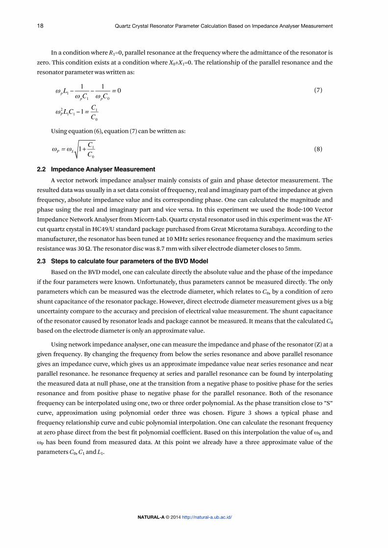
parallel resonance. he resonance frequency at series and parallel resonance can be found by interpolating
the measured data at null phase, one at the transition from a negative phase to positive phase for the series
resonance and from positive phase to negative phase for the parallel resonance. Both of the resonance
frequency can be interpolated using one, two or three order polynomial. As the phase transition close to ”S”
curve, approximation using polynomial order three was chosen. Figure 3 shows a typical phase and
frequency relationship curve and cubic polynomial interpolation. One can calculate the resonant frequency
at zero phase direct from the best fit polynomial coefficient. Based on this interpolation the value of ωS and
ωP has been found from measured data. At this point we already have a three approximate value of the
parameters C0, C1 and L1.
NATURAL-A Journal of Scientific Modeling & Computation, Volume 1 No.2 – 2014 19
ISSN 2303-0135
-90 -75 -60 -45 -30 -15 0 15 30 45 60 75 90
ω
Phase (O)
-90 -75 -60 -45 -30 -15 0 15 30 45 60 75 90
ω
Phase (O)
(a) (b)
Figure 3. Polynomial interpolation for frequency to phase;
(a) series resonance (b parallel resonance
-90 -75 -60 -45 -30 -15 0 15 30 45 60 75 90
|Z| (Ω
)
Phase
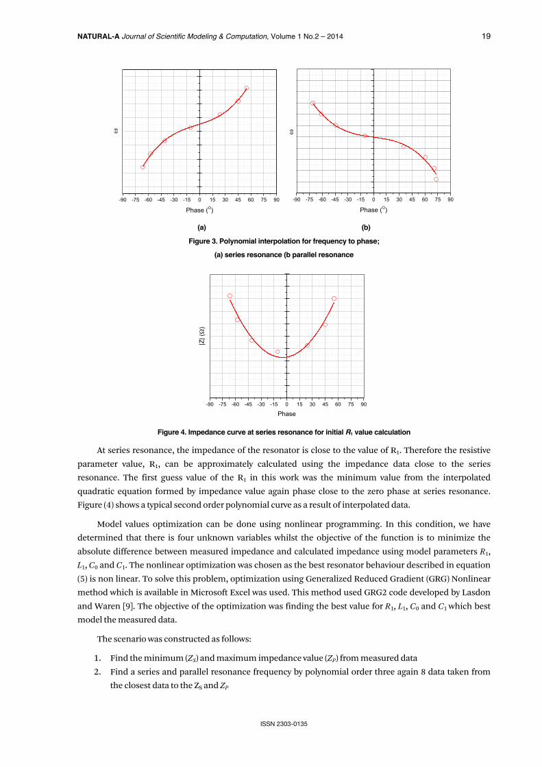
Figure 4. Impedance curve at series resonance for initial R1 value calculation
At series resonance, the impedance of the resonator is close to the value of R1. Therefore the resistive
parameter value, R1, can be approximately calculated using the impedance data close to the series
resonance. The first guess value of the R1 in this work was the minimum value from the interpolated
quadratic equation formed by impedance value again phase close to the zero phase at series resonance.
Figure (4) shows a typical second order polynomial curve as a result of interpolated data.
Model values optimization can be done using nonlinear programming. In this condition, we have
determined that there is four unknown variables whilst the objective of the function is to minimize the
absolute difference between measured impedance and calculated impedance using model parameters R1,
L1, C0 and C1. The nonlinear optimization was chosen as the best resonator behaviour described in equation
(5) is non linear. To solve this problem, optimization using Generalized Reduced Gradient (GRG) Nonlinear
method which is available in Microsoft Excel was used. This method used GRG2 code developed by Lasdon
and Waren [9]. The objective of the optimization was finding the best value for R1, L1, C0 and C1 which best
model the measured data.
The scenario was constructed as follows:
1. Find the minimum (ZS) and maximum impedance value (ZP) from measured data
2. Find a series and parallel resonance frequency by polynomial order three again 8 data taken from
the closest data to the ZS and ZP
20 Quartz Crystal Resonator Parameter Calculation Based on Impedance Analyser Measurement
NATURAL-A © 2014 http://natural-a.ub.ac.id/
3. Calculate the initial value of R1 using second orde polynomial interpolation of 8 data closest to the
series resonance
4. Calculated initial guess value for C0 series resonance frequency
5. Calculate sum of relative different from series resonance to parallel resonance (ZM: measured
impedance, ZC: Calculated impedance using BVD model)
6. Do using GRG Nonlinear Solver until minimum SE found:
a. Minimize SE by changing C0 and keeping R1 constant
b. Minimize SE by changing R1 and keeping C0 constant
The other possibility can be done by canging the sequence of GRG Nonlinear optimization on step 6
becomes:
6. Do using GRG Nonlinear Solver until minimum SE found:
a. Minimize SE by changing R1 and keeping C0 constant
b. Minimize SE by changing C0 and keeping R1 constant
3 RESULTS AND DISCUSSION We used the above described scenario to calculate the BVD parameter’s value of the resonator. From
our sample case, the initial BVD parameters value taken from measurement data followed by calculation
scenario step 1 to 4 was R1 = 6.1301416 Ω, C0 = 4.6939777 pF, C1 = 0.0229395 pF, and L1 = 11.0236714 mH.
Using this initial guess value, GRG nonlinear optimization by minimizing relative different between
measured impedance and calculated impedance at given frequency from minimum impedance to
maximum impedance points. Tabel 1 shows the change in BVD parameters according to the scenario
described above. We can see that the sum of relative different between calculated and measured impedance
was constant at step 5. Based on this condition we got the final best value of the BVD paremeters. The
parameters value was R1 = 7.4162625 Ω, C0 = 4.6115222 pF, C1 = 0.0225365 pF, and L1 = 11.2207780 mH. Slight
difference results were found by implementing alternative scenario of the GRG Nonlinear optimization. The
result of the alternative scenario was listed in Table 2. The difference between the scenario is not significant.
There was only 0.02 ppm different in R1 and 2 ppm different in C0, C1 and L1. For this work the first scenario
was used for rest of the work.
Figure 5 shows the impedance spectrum of measured data using Bode 100 Impedance analyser and
BVD model calculated using the described scenario. The measurement was done from 9.925 MHz to 10.05
MHz with receiver bandwidth at 30 Hz. Total measurement was 4096 points. This corresponding to a
frequency spacing between data was 30.25 Hz.

NATURAL-A Journal of Scientific Modeling & Computation, Volume 1 No.2 – 2014 21
ISSN 2303-0135
9.925 9.950 9.975 10.000 10.025 10.050100
101
102
103
104
105
106
|Z| (Ω
)
Frequency (MHz)
Measured |Z| Calculated |Z|
Figure 5. Impedance curve at series resonance
From Figure 5 we can see that the resulted model parameter best fitted to the measured data in a whole
spectrum. The calculated impedance spectrum was well overlaid on top of the measured impedance
spectrum. It is difficult to see the difference between both graphs. We can see that the resulted BVD
parameters can model the measured data very well.
TABLE 1. BVD PARAMATER CHANGES RESULTED BY GRG NONLINEAR OPTIMIZATION USING FIRST SCENARIO
Step Condition R1 (W) C
0 (pF) C
1 (pF) L
1 (mH) S (D)
0 Initial guess (R1, C
0, C
1, L
1) 6.1301416 4.6939777 0.0229395 11.0236714 17.6600412
1 Constant R1
6.1301416 4.6119541 0.0225386 11.2197273 6.6611161
2 Constant C0, C
1, L
1 7.4162709 4.6119541 0.0225386 11.2197273 6.3922058
3 Constant R1
7.4162709 4.6115222 0.0225365 11.2207780 6.3918131
4 Constant C0, C
1, L
1 7.4162625 4.6115222 0.0225365 11.2207780 6.3918127
5 Constant R1
7.4162625 4.6115222 0.0225365 11.2207780 6.3918127 Final Value 7.4162625 4.6115222 0.0225365 11.2207780
TABLE 2. BVD PARAMATER CHANGES RESULTED BY GRG NONLINEAR OPTIMIZATION USING SECOND SCENARIO
Step Condition R1 (W) C
0 (pF) C
1 (pF) L
1 (mH) S (D)
0 Initial guess (R1, C
0, C
1, L
1) 6.1301416 4.6939777 0.0229395 11.0236714 17.6600412
1 Constant C0, C
1, L
1 7.4177934 4.6939777 0.0229395 11.0236714 17.4302883
2 Constant R1
7.4177934 4.6115133 0.0225365 11.2207998 6.3918898
3 Constant C0, C
1, L
1 7.4162623 4.6115133 0.0225365 11.2207998 6.3918147
4 Content R1
7.4162623 4.6115133 0.0225365 11.2207998 6.3918147
5 Constant C0, C
1, L
1 7.4162623 4.6115133 0.0225365 11.2207998 6.3918147
Final Value 7.4162623 4.6115133 0.0225365 11.2207998
22 Quartz Crystal Resonator Parameter Calculation Based on Impedance Analyser Measurement
NATURAL-A © 2014 http://natural-a.ub.ac.id/
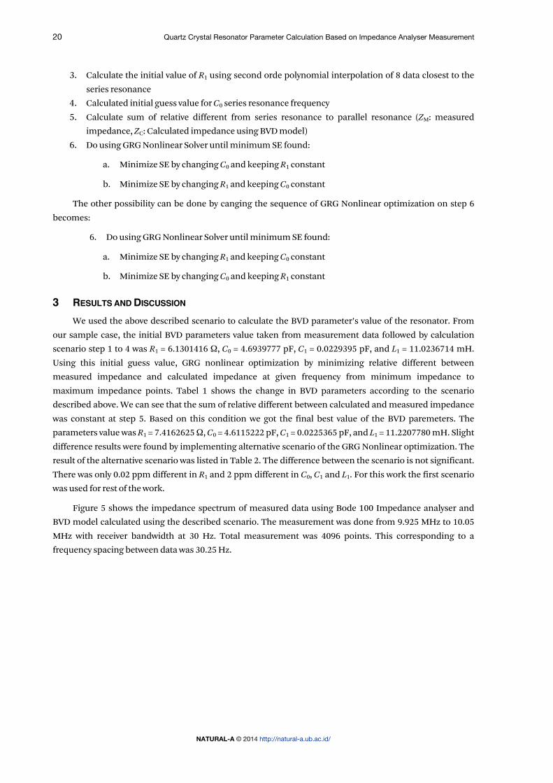
The difference between measured impedance and calculated one can be seen in Figure 6. It can be seen
that in term of absolute difference, the biggest difference exists in an impedance value close to the parallel
resonance. This magnitude can be understood well, as the absolute value of the impedance at parallel
resonance is very big. In addition, it can be seen in Figure 5 that big impedance gradient exists at parallel
resonance. Those a slight error in the frequency measurement by the impedance analyser will result in a
significant difference in the measured impedance compared to the calculated one.
The relative difference between measured impedance and calculated impedance in Figure 6 shows that
there are three peaks in the difference curve. We will focus to the first and second peaks difference. The first
one was at series resonance and the second one was at the parallel resonance. The peaks after parallel
resonance was caused by a non ideal fabrication the resonator.
9.925 9.950 9.975 10.000 10.025 10.05010-210-1100101102103104105106
0
10
20
30
40
509.925 9.950 9.975 10.000 10.025 10.050
Absolute difference
|ΔZ|
Frequency (MHz)
|ΔZ/
Z| (%
)
Relative difference
Figure 6. Absolute and relative difference of the impedance value between measured data and calculated data
At impedance close to the series resonance, the relative difference of the impedance value was high for
a few data although the absolute difference is small. This is caused by a small absolute value of the resonator
impedance. High difference at series resonance impedance was only occurring for one or two points. This
can be caused by the measurement error.
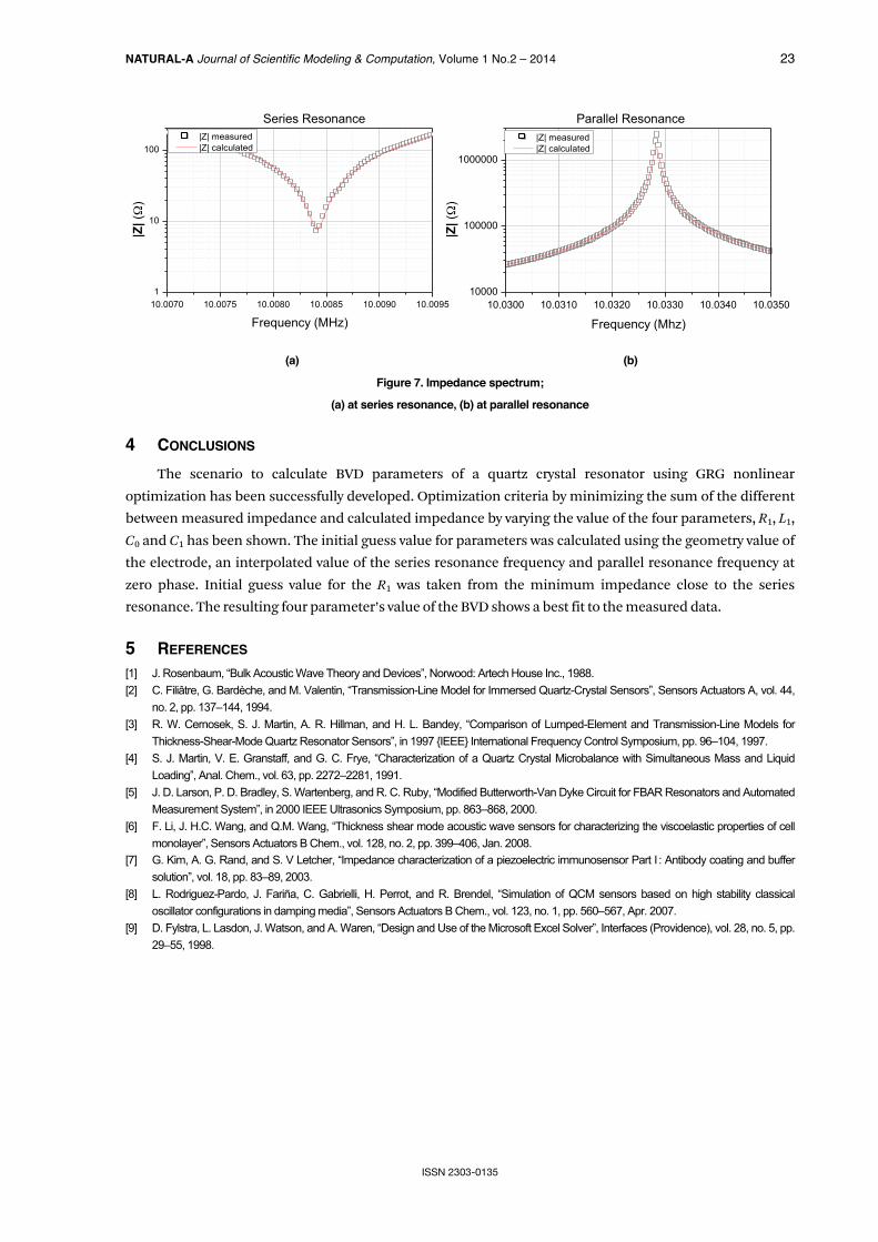
Closer look at the series and resonance frequency spectrum as shown in Figure 7 shows that the
agreement between the calculated impedance to the measured impedance existed. It can be seen from
Figure 7 that the calculated impedance spectrum well overlaid with the measured impedance. Visually there
was no significant difference between the calculated impedance and measured impedance.
NATURAL-A Journal of Scientific Modeling & Computation, Volume 1 No.2 – 2014 23
ISSN 2303-0135
10.0070 10.0075 10.0080 10.0085 10.0090 10.00951
10
100
Parallel Resonance|Z| (Ω
)
Frequency (MHz)
|Z| measured |Z| calculated
Series Resonance
10.0300 10.0310 10.0320 10.0330 10.0340 10.035010000
100000
1000000
|Z| (Ω
)
Frequency (Mhz)
|Z| measured |Z| calculated
(a) (b)
Figure 7. Impedance spectrum;
(a) at series resonance, (b) at parallel resonance
4 CONCLUSIONS The scenario to calculate BVD parameters of a quartz crystal resonator using GRG nonlinear
optimization has been successfully developed. Optimization criteria by minimizing the sum of the different
between measured impedance and calculated impedance by varying the value of the four parameters, R1, L1,
C0 and C1 has been shown. The initial guess value for parameters was calculated using the geometry value of
the electrode, an interpolated value of the series resonance frequency and parallel resonance frequency at
zero phase. Initial guess value for the R1 was taken from the minimum impedance close to the series
resonance. The resulting four parameter’s value of the BVD shows a best fit to the measured data.
5 REFERENCES
[1] J. Rosenbaum, “Bulk Acoustic Wave Theory and Devices”, Norwood: Artech House Inc., 1988. [2] C. Filiâtre, G. Bardèche, and M. Valentin, “Transmission-Line Model for Immersed Quartz-Crystal Sensors”, Sensors Actuators A, vol. 44,
no. 2, pp. 137–144, 1994. [3] R. W. Cernosek, S. J. Martin, A. R. Hillman, and H. L. Bandey, “Comparison of Lumped-Element and Transmission-Line Models for
Thickness-Shear-Mode Quartz Resonator Sensors”, in 1997 {IEEE} International Frequency Control Symposium, pp. 96–104, 1997. [4] S. J. Martin, V. E. Granstaff, and G. C. Frye, “Characterization of a Quartz Crystal Microbalance with Simultaneous Mass and Liquid
Loading”, Anal. Chem., vol. 63, pp. 2272–2281, 1991. [5] J. D. Larson, P. D. Bradley, S. Wartenberg, and R. C. Ruby, “Modified Butterworth-Van Dyke Circuit for FBAR Resonators and Automated
Measurement System”, in 2000 IEEE Ultrasonics Symposium, pp. 863–868, 2000. [6] F. Li, J. H.C. Wang, and Q.M. Wang, “Thickness shear mode acoustic wave sensors for characterizing the viscoelastic properties of cell
monolayer”, Sensors Actuators B Chem., vol. 128, no. 2, pp. 399–406, Jan. 2008. [7] G. Kim, A. G. Rand, and S. V Letcher, “Impedance characterization of a piezoelectric immunosensor Part I!: Antibody coating and buffer
solution”, vol. 18, pp. 83–89, 2003. [8] L. Rodriguez-Pardo, J. Fariña, C. Gabrielli, H. Perrot, and R. Brendel, “Simulation of QCM sensors based on high stability classical
oscillator configurations in damping media”, Sensors Actuators B Chem., vol. 123, no. 1, pp. 560–567, Apr. 2007. [9] D. Fylstra, L. Lasdon, J. Watson, and A. Waren, “Design and Use of the Microsoft Excel Solver”, Interfaces (Providence), vol. 28, no. 5, pp.
29–55, 1998.
![Quartz Crystal Oscillators with Direct Resonator HeatingCorning]_Quartz_Crystal... · 2012-03-03 · factor is hysteresis. Repeated frequency temperature curves, or curves made in](https://img.pdfslide.net/doc/110x75/5b3522137f8b9a6b548cdae5/quartz-crystal-oscillators-with-direct-resonator-heating-corningquartzcrystal.jpg)