DES-2018-0403

FERMILAB-PUB-18-621-AEDraft version February 14, 2020Typeset using LATEX twocolumn style in AASTeX62

Quasar Accretion Disk Sizes from Continuum Reverberation Mapping in the DES Standard Star Fields

Zhefu Yu,1 Paul Martini,1, 2 T. M. Davis,3, 4 R. A. Gruendl,5, 6 J. K. Hoormann,3 C. S. Kochanek,1, 2 C. Lidman,4, 7

D. Mudd,8 B. M. Peterson,1, 2, 9 W. Wester,10 S. Allam,10 J. Annis,10 J. Asorey,11 S. Avila,12 M. Banerji,13, 14

E. Bertin,15, 16 D. Brooks,17 E. Buckley-Geer,10 J. Calcino,3 A. Carnero Rosell,18, 19 D. Carollo,4, 20

M. Carrasco Kind,6, 5 J. Carretero,21 C. E. Cunha,22 C. B. D’Andrea,23 L. N. da Costa,18, 24 J. De Vicente,19

S. Desai,25 H. T. Diehl,10 P. Doel,17 T. F. Eifler,26, 27 B. Flaugher,10 P. Fosalba,28, 29 J. Frieman,30, 10

J. Garcıa-Bellido,31 E. Gaztanaga,29, 28 K. Glazebrook,32 D. Gruen,33, 22 J. Gschwend,24, 18 G. Gutierrez,10

W. G. Hartley,17, 34 S. R. Hinton,3 D. L. Hollowood,35 K. Honscheid,2, 36 B. Hoyle,37, 38 D. J. James,39 A. G. Kim,40

E. Krause,26 K. Kuehn,7 N. Kuropatkin,10 G. F. Lewis,41 M. Lima,42, 18 E. Macaulay,12 M. A. G. Maia,24, 18

J. L. Marshall,43 F. Menanteau,6, 5 R. Miquel,21, 44 A. Moller,45, 4 A. A. Plazas,27 A. K. Romer,46 E. Sanchez,19

V. Scarpine,10 M. Schubnell,47 S. Serrano,28, 29 M. Smith,48 R. C. Smith,49 M. Soares-Santos,50 F. Sobreira,18, 51

E. Suchyta,52 E. Swann,12 M. E. C. Swanson,6 G. Tarle,47 B. E. Tucker,4, 45 D. L. Tucker,10 and V. Vikram53

1Department of Astronomy, The Ohio State University, Columbus, Ohio 43210, USA2Center of Cosmology and Astro-Particle Physics, The Ohio State University, Columbus, Ohio, 43210, USA

3School of Mathematics and Physics, University of Queensland, Brisbane, QLD 4072, Australia4ARC Centre of Excellence for All-sky Astrophysics (CAASTRO), Australia

5Department of Astronomy, University of Illinois at Urbana-Champaign, 1002 W. Green Street, Urbana, IL 61801, USA6National Center for Supercomputing Applications, 1205 West Clark St., Urbana, IL 61801, USA

7Australian Astronomical Observatory, North Ryde, NSW 2113, Australia8Department of Physics and Astronomy, University of California, Irvine, Irvine, CA 92697, USA

9Space Telescope Science Institute, 3700 San Martin Drive, Baltimore, MD 21218, USA10Fermi National Accelerator Laboratory, P. O. Box 500, Batavia, IL 60510, USA

11Korea Astronomy and Space Science Institute, Yuseong-gu, Daejeon, 305-348, Korea12Institute of Cosmology and Gravitation, University of Portsmouth, Portsmouth, PO1 3FX, UK

13Kavli Institute for Cosmology, University of Cambridge, Madingley Road, Cambridge CB3 0HA, UK14Institute of Astronomy, University of Cambridge, Madingley Road, Cambridge CB3 0HA, UK

15Sorbonne Universites, UPMC Univ Paris 06, UMR 7095, Institut d’Astrophysique de Paris, F-75014, Paris, France16CNRS, UMR 7095, Institut d’Astrophysique de Paris, F-75014, Paris, France

17Department of Physics & Astronomy, University College London, Gower Street, London, WC1E 6BT, UK18Laboratorio Interinstitucional de e-Astronomia - LIneA, Rua Gal. Jose Cristino 77, Rio de Janeiro, RJ - 20921-400, Brazil

19Centro de Investigaciones Energeticas, Medioambientales y Tecnologicas (CIEMAT), Madrid, Spain20INAF, Astrophysical Observatory of Turin, Torino, Italy

21Institut de Fısica d’Altes Energies (IFAE), The Barcelona Institute of Science and Technology, Campus UAB, 08193 Bellaterra(Barcelona) Spain

22Kavli Institute for Particle Astrophysics & Cosmology, P. O. Box 2450, Stanford University, Stanford, CA 94305, USA23Department of Physics and Astronomy, University of Pennsylvania, Philadelphia, PA 19104, USA

24Observatorio Nacional, Rua Gal. Jose Cristino 77, Rio de Janeiro, RJ - 20921-400, Brazil25Department of Physics, IIT Hyderabad, Kandi, Telangana 502285, India

26Department of Astronomy/Steward Observatory, 933 North Cherry Avenue, Tucson, AZ 85721-0065, USA27Jet Propulsion Laboratory, California Institute of Technology, 4800 Oak Grove Dr., Pasadena, CA 91109, USA

28Institut d’Estudis Espacials de Catalunya (IEEC), 08034 Barcelona, Spain29Institute of Space Sciences (ICE, CSIC), Campus UAB, Carrer de Can Magrans, s/n, 08193 Barcelona, Spain

30Kavli Institute for Cosmological Physics, University of Chicago, Chicago, IL 60637, USA31Instituto de Fisica Teorica UAM/CSIC, Universidad Autonoma de Madrid, 28049 Madrid, Spain

32Centre for Astrophysics & Supercomputing, Swinburne University of Technology, Victoria 3122, Australia33SLAC National Accelerator Laboratory, Menlo Park, CA 94025, USA

34Department of Physics, ETH Zurich, Wolfgang-Pauli-Strasse 16, CH-8093 Zurich, Switzerland35Santa Cruz Institute for Particle Physics, Santa Cruz, CA 95064, USA

36Department of Physics, The Ohio State University, Columbus, OH 43210, USA37Max Planck Institute for Extraterrestrial Physics, Giessenbachstrasse, 85748 Garching, Germany

38Universitats-Sternwarte, Fakultat fur Physik, Ludwig-Maximilians Universitat Munchen, Scheinerstr. 1, 81679 Munchen, Germany39Harvard-Smithsonian Center for Astrophysics, Cambridge, MA 02138, USA

40Lawrence Berkeley National Laboratory, 1 Cyclotron Road, Berkeley, CA 94720, USA

arX

iv:1

811.

0363

8v2

[as

tro-

ph.G

A]

13

Feb

2020

2 Yu et al.

41Sydney Institute for Astronomy, School of Physics, A28, The University of Sydney, NSW 2006, Australia42Departamento de Fısica Matematica, Instituto de Fısica, Universidade de Sao Paulo, CP 66318, Sao Paulo, SP, 05314-970, Brazil

43George P. and Cynthia Woods Mitchell Institute for Fundamental Physics and Astronomy, and Department of Physics and Astronomy,Texas A&M University, College Station, TX 77843, USA

44Institucio Catalana de Recerca i Estudis Avancats, E-08010 Barcelona, Spain45The Research School of Astronomy and Astrophysics, Australian National University, ACT 2601, Australia46Department of Physics and Astronomy, Pevensey Building, University of Sussex, Brighton, BN1 9QH, UK

47Department of Physics, University of Michigan, Ann Arbor, MI 48109, USA48School of Physics and Astronomy, University of Southampton, Southampton, SO17 1BJ, UK

49Cerro Tololo Inter-American Observatory, National Optical Astronomy Observatory, Casilla 603, La Serena, Chile50Brandeis University, Physics Department, 415 South Street, Waltham MA 02453

51Instituto de Fısica Gleb Wataghin, Universidade Estadual de Campinas, 13083-859, Campinas, SP, Brazil52Computer Science and Mathematics Division, Oak Ridge National Laboratory, Oak Ridge, TN 37831

53Argonne National Laboratory, 9700 South Cass Avenue, Lemont, IL 60439, USA

ABSTRACT

Measurements of the physical properties of accretion disks in active galactic nuclei are important for

better understanding the growth and evolution of supermassive black holes. We present the accretion

disk sizes of 22 quasars from continuum reverberation mapping with data from the Dark Energy Survey

(DES) standard star fields and the supernova C fields. We construct continuum lightcurves with the

griz photometry that span five seasons of DES observations. These data sample the time variability

of the quasars with a cadence as short as one day, which corresponds to a rest frame cadence that

is a factor of a few higher than most previous work. We derive time lags between bands with both

JAVELIN and the interpolated cross-correlation function method, and fit for accretion disk sizes using

the JAVELIN Thin Disk model. These new measurements include disks around black holes with

masses as small as ∼ 107 M, which have equivalent sizes at 2500A as small as ∼ 0.1 light days in

the rest frame. We find that most objects have accretion disk sizes consistent with the prediction

of the standard thin disk model when we take disk variability into account. We have also simulated

the expected yield of accretion disk measurements under various observational scenarios for the Large

Synoptic Survey Telescope Deep Drilling Fields. We find that the number of disk measurements would

increase significantly if the default cadence is changed from three days to two days or one day.

Keywords: galaxies:active, accretion disks, quasars:general

1. INTRODUCTION

Active galactic nuclei (AGNs) are powered by an ac-

cretion disk formed by gas accreted onto a galaxy’s cen-

tral supermassive black hole (SMBH). The accretion

disk produces multi-temperature black body emission,

with a peak that is typically in the ultraviolet (UV).

Studies of the size and structure of the accretion disk are

important because they help to understand the growth

of SMBHs and the evolution of AGNs.

The conventional accretion disk model is the geomet-

rically thin, optically thick disk model (Shakura & Sun-

yaev 1973). The disk is internally heated by viscous

dissipation. Later modifications of the model include ex-

ternal heating by the UV/X-ray source near the SMBH

(e.g. Haardt & Maraschi 1991). The disk has a tem-

perature gradient, reaching about 105 − 106 K near the

center and getting colder at larger radii (e.g. Shakura

& Sunyaev 1973; Shields 1978). In this model, the tem-

perature profile has the form T (R) ∝ R−3/4 over a large

range of R, where R is the distance from the central

SMBH.

It is common to assume that the continuum is well

characterized by multi-temperature black body emis-

sion where the annulus at radius R is emitting as a

black body with temperature T (R) (e.g. Collier et al.

1998; Morgan et al. 2010; Jiang et al. 2017; Mudd et al.

2018). We consequently expect longer wavelength emis-

sion to primarily originate at larger radii. The disk size

at effective wavelength λ, defined as the position where

kT (Rλ) = hc/λ, scales with wavelength as Rλ ∝ λβ ,

where β = 4/3 in the standard thin disk model. Ac-

cretion disks are too small to be spatially resolved, and

current measurements of the size of accretion disks are

mainly from micro-lensing (e.g. Morgan et al. 2010) and

continuum reverberation mapping (e.g. Shappee et al.

2014; Fausnaugh et al. 2016; Jiang et al. 2017; Mudd

et al. 2018; Homayouni et al. 2019).

Continuum Reverberation Mapping on DES 3

Accretion disk size measurements from continuum re-

verberation mapping rely on measurements of contin-

uum lags between bands at different wavelengths. If the

variation of the continuum emission from the accretion

disk is driven by the variation of a central illuminating

source, such as the “lamppost” model (e.g. Cackett et al.

2007), the variation at longer wavelengths is expected to

lag the variation at shorter wavelengths due to the light

travel time from the inner disk to the outer disk. The

lag between two wavelengths λ and λ0 is

τ =Rλ0

c

[(λ

λ0

)β− 1

](1)

where Rλ0is the effective disk size at wavelength λ0.

Equation (1) states that the disk size is related to

the time lag between two lightcurves at different wave-

lengths. This approach to measuring the accretion disk

size is called “continuum reverberation mapping”.

One algorithm used to measure lags is the interpo-

lated cross-correlation function (ICCF), which cross-

correlates the linearly interpolated lightcurves and cal-

culates the lag as the center or peak of the cross-

correlation function (e.g. Peterson et al. 1998, 2004).

Another method is JAVELIN, which models the vari-

ability of AGNs as a damped random walk (DRW)

stochastic process and fits for the lag (e.g. Zu et al.

2011, 2013). Simply fitting the continuum lags in dif-

ferent photometric bands with the thin disk model can

provide the accretion disk size at a given wavelength.

In addition, Mudd et al. (2018) presented an alternate

method to obtain the disk size, the JAVELIN Thin Disk

model, which assumes a thin disk model from the out-

set and then fits for the thin disk parameters (Rλ0, β)

directly that best reproduce a series of lightcurves of

known effective wavelengths, instead of using the indi-

vidual lags to find a disk size through Equation (1).

Early studies to measure accretion disk sizes with con-

tinuum reverberation mapping include Wanders et al.

(1997) and Collier et al. (1998), which measured the

continuum lags of NGC 7469 at UV and visible wave-

lengths, respectively. Sergeev et al. (2005) measured

the interband lags of 14 AGNs, and found the lags scale

with the luminosity as Lb where b ≈ 0.4−0.5. Recently,

several studies obtained accurate measurements of con-

tinuum lags using intensive observations spanning from

the X-ray to the near-infrared, including Shappee et al.

(2014) for NGC 2617, Edelson et al. (2015) and Faus-

naugh et al. (2016) for NGC 5548, Edelson et al. (2017)

for NGC 4151, Cackett et al. (2018) and McHardy et al.

(2018) for NGC 4593 and Fausnaugh et al. (2018) for

MCG+08-11-011 and NGC 2617. Other studies have

used observations from large sky surveys to measure the

accretion disk sizes from larger samples. Jiang et al.

(2017) measured the continuum lags of 39 quasars using

lightcurves from Pan-STARRS. Mudd et al. (2018) used

the photometric data on the supernova fields of the Dark

Energy Survey (DES) and obtained disk sizes measure-

ments of 15 quasars. Homayouni et al. (2019) presented

the continuum lags of 95 quasars from the photometric

data for the Sloan Digital Sky Survey (SDSS) Reverber-

ation Mapping (RM) project.

Some studies, including Fausnaugh et al. (2016) and

Jiang et al. (2017), and most micro-lensing studies like

Morgan et al. (2010), found that the accretion disks are

larger than the prediction of the thin disk model by a

factor of 2 - 3. One possible explanation of the larger

disk sizes is non-thermal disk emission caused by a low

density disk atmosphere (Hall et al. 2018). Another ex-

planation is a disk wind that leads to a higher effective

temperature in the outer part of the accretion disk (e.g.

Sun et al. 2019; Li et al. 2019). Gaskell (2017) found the

internal reddening of AGNs that leads to an underesti-

mation of the far-UV luminosity can be an explanation

of the discrepancy as well. Contamination by the dif-

fuse continuum from the broad line region (BLR) (e.g.

Korista & Goad 2001; Lawther et al. 2018) may lead

to larger disk size measurements from continuum rever-

beration mapping. In addition, an inhomogeneous disk

with significant local temperature fluctuations may also

explain the larger disk sizes from micro-lensing studies

(Dexter & Agol 2011). However, Mudd et al. (2018)

and Homayouni et al. (2019) did not find systematic

trends of larger disk sizes than the prediction of the

thin disk model. To address this discrepancy, more disk

size measurements are required, especially using high-

cadence time series data.

In this paper, we present disk size measurements us-

ing the photometric data in the DES standard star fieldsand the supernova C (SN-C) fields. The structure of this

paper is as follows. Section 2 introduces the photomet-

ric data we use. Section 3 introduces the methodology

and results of the time series analysis, including the lag

and disk size measurements. In Section 4 we discuss

various tests we performed to verify the measurements.

In Section 5 we describe our measurements of the cor-

relation between the accretion disk size and the mass

of the SMBH. Section 6 discusses the objects without

lag measurements. In Section 7 we present simulations

of the Large Synoptic Survey Telescope Deep Drilling

Fields and quantify the effect of observational cadence

on lag measurements. Section 8 summarizes the paper.

Throughout the paper we adopt ΛCDM cosmology with

H0 = 70 km/s/Mpc, Ωm = 0.3, ΩΛ = 0.7.

4 Yu et al.

2. OBSERVATIONS

DES is a ground-based, wide-area, visible and the

near-infrared imaging survey (Abbott et al. 2018). DES

started Commissioning and Science Verification (SV)

observations in 2012, and the main survey began in

2013. DES uses the Dark Energy Survey Camera

(DECam), a 570 megapixel, 2.2 field of view cam-

era installed on the 4-m Victor M. Blanco telescope at

the Cerro Tololo Inter-American Observatory (Flaugher

et al. 2015). DES includes a 5000 deg2 wide-area survey

in the grizY bands, and 27 deg2 in the griz bands that

are repeatedly imaged to identify and characterize su-

pernova. DES typically observes standard star fields in

morning and evening twilight for calibration, and occa-

sionally around midnight as well. Standard star obser-

vations can have a nightly or even higher observational

cadence in some fields, with a typical exposure time of

15 seconds for a single epoch. The high observational

cadence supports accurate photometric RM analysis, de-

spite the short exposure time.

We use standard star observations from the DES SV

period through Year 4 (Y4) in the MaxVis field, the

C26202 fields, and 6 other fields within the SDSS foot-

print. We incorporate spectroscopic data for the MaxVis

and the C26202 fields from the Australian DES/Optical

redshifts for DES (OzDES) program, a spectroscopic

survey with the Anglo-Australian Telescope that was de-

signed to follow up targets identified from DES (Yuan

et al. 2015; Childress et al. 2017).

2.1. MaxVis Field

The MaxVis field is centered at RA = 97.5, DEC =

−58.75. The field is observable throughout the DES ob-

serving season, and it was named because of this “Max-

imum Visibility”. We visually inspected all OzDES

spectra flagged as non-stellar within the field, and se-

lected 130 quasars as candidates with spectroscopic

redshifts from OzDES Global Redshift Catalog (Chil-

dress et al. 2017). The cyan histogram in Figure 1

shows the observational cadence distribution of DES

J063037.48−575610.30, a representative object in the

MaxVis field. The distribution peaks around one day,

indicating that most epochs for this object are obtained

with a nearly daily cadence. The orange squares in Fig-

ure 2 shows the magnitude uncertainty as a function of

the g-band magnitude for the quasars in the MaxVis

field. The depth of the MaxVis field is intermediate rel-

ative to the other standard star fields.

2.2. SDSS Stripe 82 Fields

We use six fields near the celestial equator that over-

lap the SDSS Stripe 82 field (e.g. Adelman-McCarthy

0 2 4 6 8 10 12 14Observation Interval (days, g band)

0

10

20

30

40

50

60

70 MaxVisSDSSC26202SN-C

Figure 1. Time interval distribution between consecutive pairs

of epochs for the lightcurve of a representative object in each field.

The cyan filled, black dotted, red solid and blue dashed histograms

are the cadence distribution of DES J063037.48−575610.30 in

the MaxVis field, DES J005905.51+000651.66 in the SDSS

fields, DES J033408.25−274337.81 in the C26202 field and DES

J034001.53−274036.91 in the SN-C fields, respectively.

16 17 18 19 20 21 22 23Magnitude (g band)

0.00

0.02

0.04

0.06

0.08

0.10

0.12

0.14Magnitude Erro

r (g band

)SDSSC26202SN-CMaxVis

Figure 2. Magnitude uncertainty as a function of magnitude for

g-band data for the four datasets. The orange squares, black cir-

cles, red crosses and green pentagons represent the objects in the

MaxVis, the SDSS, the C26202 and the SN-C fields, respectively.

The magnitude shown here is calculated as the mean magnitude

of the object from SV to Y4, and the magnitude uncertainty is

calculated as the mean magnitude uncertainty during this period.

The magnitude uncertainties have included the calibration errors.

et al. 2007). We match DES observations to the color

and variability selected quasar catalog from Peters et al.

(2015), and select 884 objects as candidates with more

than 200 epochs in the grizY bands from SV to Y4,

among which 593 objects have spectroscopic redshifts.

Similar to the MaxVis field, Figure 1 shows that the ob-

servational cadence in the SDSS fields is roughly daily.

On the other hand, Figure 2 shows that the observations

in the SDSS fields are shallower compared to the other

fields.

Continuum Reverberation Mapping on DES 5

2.3. C26202 and SN-C Fields

The C26202 field is centered on the standard star

C26202 at RA = 53.1, DEC = −27.85, which over-

laps with the DES C1, C2 and C3 supernova fields. We

match the DES detections within a circle of 3.5 radius

to the spectroscopically confirmed quasar catalog pre-

sented by Tie et al. (2017), and selected 318 quasars as

candidates with more than 200 epochs in the griz bands

from SV to Y4. Note that the candidates include not

only quasars from the C26202 standard star field, but

also quasars within the SN-C fields. The DES obser-

vations of the C26202 standard star field include both

approximately daily standard star observations and ap-

proximately weekly supernova observations. Figure 1

shows the cadence distribution of a representative object

in this field, where most observations are high-cadence

standard star observations shown by the peak around

one day, while there are also supernova observations

with longer intervals between epochs. Figure 2 shows

that quasars within the C26202 standard star field have

the deepest observations (the red crosses) compared to

the quasars within the other two, while the observa-

tions of quasars within the supernova fields (the green

pentagons) are even deeper. Hereafter we use “C26202

fields” to refer to both the C26202 standard star field

and the SN-C fields unless otherwise specified.

3. TIME SERIES ANALYSIS

We construct lightcurves using photometric data from

the DES Y4A1 catalogs. We adopt the PSF magnitude

and its error for the photometry, and exclude bad epochs

based on the DES data quality flags. For time series

analysis, the calibration between epochs would add ad-

ditional systematic errors. We adopt the typical error of

the DES Forward Global Calibration Method (FGCM)

from Burke et al. (2018) and combine it with the magni-

tude errors by quadrature to calculate the total uncer-

tainty of each single epoch.

There are epochs separated by only minutes, which

can be caused by the short acquisition images or the cos-

mic ray separation of the supernova observations. Since

the variations between these epochs are not likely to be

intrinsic to the quasars, we exclude the short acquisition

epochs and combine the supernova epochs separated by

less than half hour to avoid possible artifacts in further

analysis. We assume that the seeing and the sky trans-

parency do not vary significantly within this time range,

and calculate the magnitude and magnitude error of the

combined epoch as

mcomb =

∑i

mi/σ2i∑

i

1/σ2i

, σ2comb =

1∑i

1/σ2i

(2)

where mi and σi are the magnitude and its statistical

error of each single epoch. We combine σcomb with the

calibration error by quadrature to calculate the total

uncertainty of the combined epoch.

We assess the variability of an object by calculating a

χ2 value defined as

χ2 =∑X

∑i

(mi,X −mX

σi,X

)2

(3)

where mi,X and σi,X represents the magnitude and un-

certainty of the ith data point in band X (X=g,r,i,z,Y ),

and mX represents the mean magnitude in band X. We

calculate the χ2 values both for the whole SV - Y4 pe-

riod and for the single seasons. We perform a time se-

ries analysis on objects and seasons that satisfy: (1)

Nfit > 100, where Nfit is the number of epochs in the

season to analyze; (2) Nother > 200, where Nother is the

number of epochs in all the other seasons that are not

analyzed; and (3) χ2r > 2, indicating significant vari-

ability, where χ2r = χ2/(Nfit − 5) is the reduced χ2.

There are 48 objects in the MaxVis field, 457 objects

in the SDSS fields and 297 objects in the C26202 fields

that met the criteria in at least one observational sea-

son. Among these objects, about half of the objects

in the MaxVis field and the SDSS fields have only one

season that met the criteria, while most objects in the

C26202 fields have at least two seasons. We analyze

each season that passed the selection independently for

computational convenience when measuring time lags.

Quasars can have lag detections from multiple seasons,

and we discuss this further in Section 3.1.

Figure 3 shows χ2r as a function of the number of

epochs for the candidates. The quasars within the SDSS

fields show the smallest variations relative to the pho-

tometric errors, while many quasars in the SN-C field

have large χ2r due to the deep supernova observations.

In this work, we use JAVELIN, the JAVELIN Thin

Disk model, and the ICCF method to measure lags and

derive disk sizes. We obtain good quality disk size mea-

surements for 22 quasars. We refer to these quasars

as the “main sample”. The basic properties of these

quasars are listed in Table 1, and disk size results are

presented in Table 2. Seventeen of the 22 quasars form

the most reliable subset of the measurements. The re-

maining five are flagged due to inconsistencies of lags

either between the observational seasons (flag = 1) or

the analysis methods (flag = 2), or simulation results

that imply lower reliability based on the observational

data and an estimate of the disk size (flag = 3). The

process of assigning flags is described in the next sec-

tions. We separate objects with and without flags in

Table 2.

6 Yu et al.

0 50 100 150 200 250 300 350Number of epochs

100

101

102

103Re

duced χ2

MaxVisSDSSC26202SN-C

Figure 3. χ2r as a function of the number of epochs. The or-

ange squares, black circles, red diamonds and green pentagons

represent the objects from the MaxVis field, the SDSS fields, the

C26202 standard star field, and the SN-C fields, respectively. The

small symbols represent the objects where we do not obtain good

lag measurements. The large symbols represent the objects in

the main sample with the empty symbols for the flagged objects.

For the objects without lag measurements, χ2r and the number

of epochs are calculated from the season where χ2r is the largest.

For objects in the main sample, χ2r and the number of epochs are

from the season where the lags and disk sizes are measured. If

an object has lag measurements from multiple seasons, χ2r is from

the earliest season that has lag measurements. The horizontal red

dashed line is drawn at χ2r = 2, and the vertical line is drawn at

Nfit = 100.

Figure 4 shows the lightcurves of six randomly selected

unflagged objects in the observational season from which

we obtain lag measurements. We present the lightcurve

data and plots in the online journal for all seasons and

objects in the main sample.

3.1. JAVELIN Analysis

We use JAVELIN (Zu et al. 2011) to model quasar

variability as a DRW. The covariance function of a DRW

has an exponential form

S(∆t) = σ2DRW exp(−|∆t/τDRW|) (4)

where ∆t is the time interval between two epochs,

σDRW is the amplitude, and τDRW is the characteristic

time scale. Previous studies have shown that quasar

lightcurves are generally well described by a DRW (e.g.

Kelly et al. 2009; Koz lowski et al. 2010; MacLeod et al.

2010; Zu et al. 2013). However, several studies found

that the Kepler lightcurves of AGNs show steeper power

spectral density (PSD) than the DRW model at time

scales shorter than ∼ month (e.g. Mushotzky et al. 2011;

Smith et al. 2018). Here we use JAVELIN with the

awareness of the potential effect of this deviation from

DRW.

Table 1. Quasars in the Main Sample

Object Name z Field Reference Line MBH

(108M)

DES J063037.48−575610.30 0.43 MaxVis Hβ 1.23

DES J063510.91−585303.70 0.22 MaxVis Hβ 0.23

DES J063159.74−590900.60 0.73 MaxVis Mg II 2.00

DES J062758.99−582929.60 0.49 MaxVis Hβ 0.20

DES J033002.93−273248.30 0.53 C26202 Hβ 0.80

DES J033408.25−274337.81 1.03 C26202 Mg II 1.18

DES J034003.89−264524.52 0.49 C26202 Hβ 0.44

DES J032724.94−274202.81 0.76 C26202 Mg II 1.71

DES J033545.58−293216.51 0.72 C26202 Mg II 0.82

DES J033810.61−264325.00 0.85 C26202 Mg II 2.05

DES J034001.53−274036.91 1.15 C26202 Mg II 1.98

DES J033853.20−261454.82 1.17 C26202 Mg II 2.65

DES J033051.45−271254.90 0.63 C26202 Hβ 0.61

DES J032853.99−281706.90 1.00 C26202 Mg II 5.65

DES J032801.84−273815.72 1.59 C26202 Mg II 3.28

DES J033230.63−284750.39 0.86 C26202 Mg II 1.49

DES J033729.20−294917.51 1.35 C26202 Mg II 1.95

DES J033220.03−285343.40 1.27 C26202 Mg II 1.37

DES J033342.30−285955.72 0.55 C26202 Hβ 2.05

DES J033052.19−274926.80 1.95 C26202 C IV 0.98

DES J033238.11−273945.11 0.84 C26202 Mg II 1.33

DES J005905.51+000651.66 0.72 SDSS Hβ 8.87

Note—Basic parameters of the DES quasars in the main sample. Column (1) givesthe names of the objects. Column (2) gives the redshifts. Column (3) gives thefield names. Column (4) gives the emission lines used to estimate to black holemass, and Column (5) gives the single-epoch estimate of the black hole mass(See Section 5). The uncertainty of the black hole mass is about 0.4 dex.

JAVELIN first fits the continuum lightcurve, which

can be the lightcurve in any of the broad bands in contin-

uum RM, to constrain σDRW and τDRW. Then JAVELIN

assumes that the line lightcurve, which in our case is

the lightcurve in another continuum band, is a shifted,

smoothed and scaled version of the first lightcurve. This

fits three additional parameters: the time lag, the top-

hat smoothing factor and the flux scaling factor. We

fix τDRW to the value from the g-band continuum fitting

when fitting for the time lag of most objects, since in the

case of an accretion disk the time lag is much smallerthan the time scale of the DRW and the fitting result is

insensitive to τDRW.

Figures 5 - 8 show the probability distribution of time

lags of the r, i and z bands relative to the g band. Fig-

ures 5 - 7 only include objects without flags, while Figure

8 shows flagged objects. In most cases there is a single,

clear peak in the lag distribution. While the distribu-

tions show secondary peaks in some objects, the ampli-

tude of the secondary peak is very small compared to the

main peak. Objects from the MaxVis field, whose obser-

vational cadence is around 1-day, produce lags with sig-

nificantly smaller uncertainty compared to some of the

objects in the C26202 field with about a 7-day cadence.

We adopt the median of the probability distribution as

the best-fit lag, and the 16th and 84th percentile of the

distribution as the 1σ lower and upper limit of the lag,

Continuum Reverberation Mapping on DES 7

540 560 580 600 620 640 660 680 700

19.0

19.5

DES J034003.89-264524.52 (C26202,Y1)g r i z

1625 1650 1675 1700 1725 1750 1775 1800

21.0

21.5

DES J033220.03-285343.40 (C26202,Y4)

540 560 580 600 620 640 660 680 700

20.5

21.0

DES J034001.53-274036.91 (C26202,Y1)

240 250 260 270 280 290 300 310

19.00

19.25

DES J063159.74-590900.60 (MaxVis,SV)

540 560 580 600 620 640 660 680 700

19.4

19.6

DES J033810.61-264325.00 (C26202,Y1)

1250 1275 1300 1325 1350 1375 1400 1425MJD-56000

19.75

20.00

DES J032853.99-281706.90 (C26202,Y3)

DES

Mag

nitu

des

Figure 4. DES lightcurves of a randomly selected subset of the unflagged objects in the main sample. The object’s name, field and the

observational season(s) from which we measure the lag is shown in the upper left corner of each row. The green circles, red squares, blue

diamonds, black hexagons and yellow pentagons represent the g, r, i, z and Y data, respectively. The green, red, blue and black arrows

point to the approximate positions of the features that show visible lags in the g, r, i and z -band lightcurves, respectively.

8 Yu et al.

respectively. We provide more detailed comments on

individual objects in the Appendix.

We also use the JAVELIN Thin Disk model extension

developed by Mudd et al. (2018) to measure the accre-

tion disk size Rλ0and index β in Equation (1) using all

four bands simultaneously. The JAVELIN Thin Disk

model makes use of the information from photometric

lightcurves in all bands to better constrain the accretion

disk size, and reduces the number of parameters. Sim-

ilar to Mudd et al. (2018), we find that the JAVELIN

Thin Disk model could not well-constrain both Rλ0and

β at the same time, so we fix β = 4/3 during the fit-

ting. We again fix τDRW. Figure 9 and Figure 10 show

the probability distribution of the g-band accretion disk

size Rg in the observed frame, i.e. the disk size at

λ = 4730(1+z) A, where z is the redshift. Figure 9 only

includes objects without flags, while Figure 10 shows

flagged objects. Again, most distributions show clear

single peaks. We convert the g-band disk size to rest

frame 2500 A assuming Rλ ∝ λ4/3 for comparison with

other studies.

We inspected the lag distributions from JAVELIN and

the disk size distributions from the JAVELIN Thin Disk

model for all candidates that satisfied the criteria in

Section 3. We define a successful measurement of the

single-band lag or the accretion disk size if the probabil-

ity distributions satisfy three criteria: (1) The 1σ lower

limit of the lag or disk size is larger than zero; (2) The

probability distribution shows a clear single peak with-

out significant secondary peaks. We define a secondary

peak to be “significant” if its peak probability density

is more than 20% of the main peak. Secondary peaks

may also be a “bump” in the main peak. We treat a

“bump” as a secondary peak if it is separated from the

main peak by at least 0.75 days, and the probability

density difference between the bump peak and where it

connects the main peak is larger than 7.5% of the main

peak. (3) The 1σ upper limit of the top-hat smoothing

factor is smaller than 30. We added the third criterion

because large smoothing factors are usually related to

smooth lag distributions without clear peaks, which is

a common feature of the failed fits from JAVELIN. We

define successful measurements for an object in an obser-

vational season if the lag distributions in at least one of

the riz bands and the disk size distributions satisfy the

successful measurement criteria. We identify 22 quasars

to have successful lag and disk size measurements in

at least one observational season, and we refer to these

quasars as the “main sample”. Table 1 lists some of

the basic parameters of the quasars in the main sample.

Table 2 shows the best-fit lag and the 1σ errors from

JAVELIN in Columns (2)-(4), and the 2500A accretion

disk size in Column (5). While the selection criteria re-

quires positive lags in only one band, nearly all of the

quasars in the main sample have positive lags in at least

two of the riz bands relative to the g band.

Table 2. Lags and Accretion Disk Sizes

Object Name(Season) τr τi τz R2500A

flag Visible

(days) (days) (days) (lt-days) lag

DES J0630−5756(SV) 2.2+0.2−0.9

2.3+0.1−0.4

2.4+0.1−0.1

0.76+0.04−0.04

0 Y

DES J0635−5853(SV) 0.4+0.1−0.1

0.5+0.1−0.1

0.5+0.1−0.1

0.14+0.03−0.04

0 N

DES J0631−5909(SV) 3.4+2.4−2.2

4.0+1.7−1.0

5.2+1.7−0.9

1.81+0.41−0.28

0 Y

DES J0340−2645(Y1) 0.4+0.4−0.4

1.7+0.5−0.6

2.1+0.5−0.7

0.74+0.15−0.16

0 Y

DES J0327−2742(Y3,4) 1.2+0.9−0.9

2.6+1.0−0.9

4.7+1.6−1.4

1.53+0.47−0.46

0 Y

DES J0335−2932(Y1,3) 1.9+0.7−0.6

2.0+0.5−0.5

1.9+0.7−0.6

0.83+0.25−0.23

0 Y

DES J0338−2643(Y1,2,3) 3.3+0.8−0.9

0.9+1.0−1.1

5.9+1.2−1.1

1.54+0.39−0.41

0 Y

DES J0340−2740(Y1) 3.7+1.3−1.2

4.3+1.1−1.0

5.6+0.6−1.0

1.96+0.28−0.52

0 Y

DES J0338−2614(Y3) 0.7+0.6−0.6

1.1+0.6−0.7

1.1+0.7−0.7

0.40+0.24−0.32

0 N

DES J0330−2712(SV) 1.4+1.9−1.2

2.3+1.8−1.2

3.2+1.8−1.7

1.03+0.55−0.47

0 Y

DES J0328−2817(Y3,4) 2.5+0.7−0.7

4.8+0.9−1.0

6.7+1.2−1.2

2.46+0.44−0.48

0 Y

DES J0332−2847(Y4) 0.8+0.6−0.5

1.9+0.5−0.6

2.2+0.7−0.6

0.86+0.24−0.23

0 N

DES J0337−2949(Y4) 2.0+1.3−1.2

2.5+0.9−0.9

NaN 1.51+0.58−0.58

0 N

DES J0332−2853(Y4) 3.1+0.9−1.0

3.9+0.8−0.8

3.0+0.8−0.8

1.40+0.32−0.33

0 Y

DES J0333−2859(Y4) 0.6+0.6−0.4

3.3+0.6−0.7

3.7+0.5−0.6

1.26+0.19−0.37

0 Y

DES J0330−2749(Y4) 1.7+1.7−1.6

2.5+1.7−1.6

NaN 1.67+1.13−1.10

0 N

DES J0332−2739(Y2,3,4) 1.4+1.3−1.2

3.1+1.5−1.5

3.3+1.4−1.3

1.28+0.47−0.47

0 Y

DES J0627−5829(SV) 1.8+1.9−1.1

2.0+1.9−1.1

2.0+1.9−1.0

0.15+0.11−0.12

23 Y

DES J0330−2732(Y1) 1.1+1.4−1.3

1.8+0.9−0.8

2.9+0.7−0.6

0.97+0.18−0.15

2 N

DES J0334−2743(Y2,3) 1.5+0.6−0.6

4.5+0.6−0.7

3.9+0.7−0.6

1.66+0.13−0.28

12 N

DES J0328−2738(Y1,2) 3.7+1.7−1.3

7.7+1.1−1.2

NaN 4.78+1.31−0.94

2 Y

DES J0059+0006(Y2) 3.4+0.4−2.0

2.4+0.4−0.9

2.7+0.6−0.3

0.78+0.05−0.07

2 N

Note—Columns (2)-(4) give the JAVELIN r, i and z band lags relative to the gband and their 1σ uncertainties. “NaN” values mean that we do have goodlag measurements in this band. Column (5) gives the accretion disk sizes fromthe JAVELIN Thin Disk model with 1σ error bars. Column (6) gives the flagsindicating the issues to note for the object. flag = 0 means no issue to note.flag = 1 means that the object has lag measurements in multiple seasons thatare not consistent with each other. flag = 2 means we cannot obtain good lagsfor the object with the ICCF method (see Section 3.2). flag = 3 indicates thelightcurve of the object are not likely to provide good lag measurements givenits cadence and depth based on simulation (see Section 4.1). Column (7) giveswhether the lag signal can be visually seen from the lightcurve of the object,where “Y” means the lag is visible while “N” means the lag is not clear in thelightcurve (see Section 3.3).

As is shown in Figure 3, all of the quasars in the

main sample have either a large χ2r, implicating signifi-

cant variability relative to the photometric errors, or a

large number of epochs, corresponding to a high obser-

vational cadence. Most candidates in the SDSS fields

have smaller χ2r than those in the main sample, which

may explain why only one quasar from the SDSS fields

is in the main sample, even though these fields have so

many quasars.

We treat the observations in each season as inde-

pendent time series and analyze them separately with

JAVELIN. Column (1) in Table 2 shows the seasons

where we obtain good measurements for each ob-

Continuum Reverberation Mapping on DES 9

−5.0 −2.5 0.0 2.5 5.0 7.50

1

2

3 DES J063037.48-575610.30JAVELINICCF(cen()ICCF(peak)

−5.0 −2.5 0.0 2.5 5.0 7.50

1

2

−5.0 −2.5 0.0 2.5 5.0 7.50

2

4

−5.0 −2.5 0.0 2.5 5.0 7.50

2

4DES J063510.91-585303.70

−5.0 −2.5 0.0 2.5 5.0 7.50

2

4

−5.0 −2.5 0.0 2.5 5.0 7.50

2

4

−10 0 100.0

0.1

0.2 DES J063159.74-590900.60

−10 0 100.0

0.2

0.4

−10 0 100.0

0.2

0.4

−10 0 100.0

0.5

1.0DES J034003.89-264524.52

−10 0 100.0

0.5

1.0

−10 0 100.0

0.5

1.0

−10 0 100.0

0.2

0.4

0.6 DES J032724.94-274202.81

−10 0 100.0

0.2

0.4

−10 0 100.0

0.1

0.2

0.3

−10 0 10la (da)s, r band)

0.00

0.25

0.50

0.75 DES J033545.58-293216.51

−10 0 10la (da)s, i band)

0.0

0.5

1.0

−10 0 10la (da)s, z band)

0.0

0.2

0.4

0.6

Figure 5. Probability distributions of time lags for quasars without flags in the main sample. Each row represents the results for one

object whose name is listed in the upper left corner of the first panel, with the first, second and third columns representing the lags in the

r, i and z band relative to g band, respectively. In each panel, the blue solid line is the lag distribution from JAVELIN, while the red

dash-dotted line and the black dashed line represent the ICCF center and peak distribution, respectively.

10 Yu et al.

−10 0 100.0

0.2

0.4

0.6DES J033810.61-264325.00

JAVELINICCF(cen()ICCF(peak)

−10 0 100.0

0.2

0.4

−10 0 100.0

0.2

0.4

−10 0 100.0

0.2

0.4 DES J034001.53-274036.91

−10 0 100.0

0.2

0.4

−10 0 100.00

0.25

0.50

0.75

−10 0 100.00

0.25

0.50

0.75 DES J033853.20-261454.82

−10 0 100.00

0.25

0.50

0.75

−10 0 100.0

0.2

0.4

0.6

0.8

−10 0 100.0

0.2

0.4 DES J033051.45-271254.90

−10 0 100.0

0.1

0.2

0.3

−10 0 100.0

0.1

0.2

0.3

−10 0 100.0

0.2

0.4

0.6 DES J032853.99-281706.90

−10 0 100.0

0.2

0.4

0.6

−10 0 100.0

0.2

0.4

−10 0 10la (da)s, r band)

0.00

0.25

0.50

0.75DES J033230.63-284750.39

−10 0 10la (da)s, i band)

0.00

0.25

0.50

0.75

−10 0 10la (da)s, z band)

0.00

0.25

0.50

0.75

Figure 6. Figure 5, continued.

Continuum Reverberation Mapping on DES 11

−10 0 100.0

0.2

0.4

0.6DES J033729.20-294917.51

JAVELINICCF(cen()ICCF(peak)

−10 0 100.0

0.2

0.4

−10 0 100.0

0.2

0.4

DES J033220.03-285343.40

−10 0 100.0

0.2

0.4

0.6

−10 0 100.0

0.2

0.4

0.6

−10 0 100.0

0.5

1.0DES J033342.30-285955.72

−10 0 100.00

0.25

0.50

0.75

−10 0 100.0

0.5

1.0

−10 0 100.0

0.2

0.4 DES J033052.19-274926.80

−10 0 100.0

0.1

0.2

0.3

−10 0 10la (da)s, r band)

0.0

0.2

0.4DES J033238.11-273945.11

−10 0 10la (da)s, i band)

0.0

0.1

0.2

0.3

−10 0 10la (da)s, z band)

0.0

0.2

0.4

Figure 7. Figure 5, continued.

ject. There are seven objects that have good mea-

surements in multiple seasons. We compare the ac-

cretion disk sizes from different seasons in Figure 11.

Most objects show consistent disk sizes from different

seasons at the 1σ level, while only one object (DES

J033408.25−274337.81) shows different disk sizes from

the different seasons. For these objects, we show

the lags and disk sizes from fitting the lightcurves

in all seasons simultaneously in Table 2 and adopt

them for further analysis. We add flag = 1 to DES

J033408.25−274337.81 in Table 2. The discrepancy in

the disk sizes from different seasons may be because the

accretion disk undergoes structural changes between

seasons, or that the time lags between different photo-

metric bands are not exactly described by the simple

scenario that we assumed.

12 Yu et al.

−10 0 100.0

0.2

0.4DES J062758.99-582929.60

JAVELINICCF(c nt)ICCF(peak)

−10 0 100.0

0.2

0.4

−10 0 100.0

0.2

0.4

−10 0 100.0

0.1

0.2

0.3DES J033002.93-273248.30

−10 0 100.0

0.2

0.4

0.6

−10 0 100.00

0.25

0.50

0.75

−10 0 100.00

0.25

0.50

0.75DES J033408.25-274337.81

−10 0 100.00

0.25

0.50

0.75

−10 0 100.00

0.25

0.50

0.75

−10 0 100.0

0.1

0.2

0.3DES J032801.84-273815.72

−10 0 100.0

0.2

0.4

−10 0 10lag(day(, r band)

0.0

0.5

1.0DES J005905.51+000651.66

,10 0 10lag(day(, i band)

0.0

0.5

1.0

,10 0 10lag(day(, + band)

0.0

0.5

1.0

1.5

Figure 8. Same as Figures 5 - 7, but for quasars with flags in the main sample.

A successful lag measurement in one season does not

guarantee successful lag measurements in other seasons.

There are three factors that can prevent a lag mea-

surement in a given season: the AGN variability, the

lightcurve photometric data quality and the observa-

tional cadence. A successful lag measurement, and par-

ticularly one easily confirmed by visual inspection, re-

quires a significant flux variation relative to the photo-

metric errors that is also well-sampled by the observa-

tional cadence. AGN variability is sufficiently stochastic

that the largest photometric variations may fall outside

of the range of the lightcurve data, be on order the pho-

tometric noise (or less), or be insufficiently well sampled

to identify a clear signal. For example, less than a quar-

ter of the objects in the MaxVis and SDSS fields meet

our selection criteria (Section 3) in more than one sea-

Continuum Reverberation Mapping on DES 13

1.2 1.4 1.6 1.80

2

4

6DES J063037.48-575610.30

−0.2 0.0 0.2 0.4 0.60

2

4

6

8DES J063510.91-585303.70

−4 −2 0 2 4 60.0

0.2

0.4

0.6

0.8 DES J063159.74-590900.60

1 2 30.00

0.25

0.50

0.75

1.00

1.25

1.50 DES J034003.89-264524.52

0 2 4 60.0

0.1

0.2

0.3

0.4

0.5DES J032724.94-274202.81

−2 0 2 40.0

0.2

0.4

0.6

0.8

1.0DES J033545.58-293216.51

0 2 4 60.0

0.2

0.4

0.6DES J033810.61-264325.00

1 2 3 4 5 60.0

0.2

0.4

0.6

0.8DES J034001.53-274036.91

−1 0 1 20.0

0.2

0.4

0.6

0.8

1.0

1.2DES J033853.20-261454.82

−4 −2 0 2 4 60.0

0.1

0.2

0.3

0.4

0.5 DES J033051.45-271254.90

2 4 60.0

0.1

0.2

0.3

0.4

0.5

0.6DES J032853.99-281706.90

−1 0 1 2 30.0

0.2

0.4

0.6

0.8

1.0

1.2DES J033230.63-284750.39

−2 0 2 4 60.0

0.1

0.2

0.3

0.4

0.5DES J033729.20-294917.51

0 2 40.0

0.2

0.4

0.6

0.8DES J033220.03-285343.40

1 2 3 40.0

0.2

0.4

0.6

0.8

1.0

1.2 DES J033342.30-285955.72

−5 0 5 100.00

0.05

0.10

0.15

0.20

0.25 DES J033052.19-274926.80

0 2 4 6Rg (lt-days)

0.0

0.1

0.2

0.3

0.4

0.5 DES J033238.11-273945.11

Figure 9. Probability distributions for the observed frame g-band accretion disk sizes from the JAVELIN Thin Disk model for quasars

without flags in the main sample. Each panel shows the result for one object.

14 Yu et al.

son, while the other seasons do not have enough epochs

and/or sufficient lightcurve data quality (signal-to-noise

ratio).

The variability of the broad emission lines can contam-

inate the continuum lag measurements. The variations

of broad emission lines lag the continuum due to the

light travel time from the accretion disk to the BLR. The

broad line variability may consequently make the mea-

sured lag larger than the real continuum lag. We assess

the contamination from broad emission lines as the ratio

of the equivalent width of the emission line to the effec-

tive width of the broad band filter, referred to as fBLR,

similar to Homayouni et al. (2019). Those authors iden-

tified potential contamination if fBLR > 12.5%. For

each object in the main sample in the MaxVis and the

C26202 fields, we calculated the fBLR for the Lyα, C IV,

C III], Mg II, Hβ and Hα if the line fell into the band

pass of any of the g, r, i or z bands. For the object

within the SDSS footprint, we adopted the equivalent

width of the emission lines from Shen et al. (2011). We

show fBLR as a function of redshift for the g, r, i and

z bands in Figure 12. All objects show fBLR less than

12.5%, indicating that our continuum lag measurements

have little contamination from broad lines. There are a

few lines where we did not derive fBLR because the line

falls out of the wavelength range of the OzDES spectrum

from 3700 A to 8800 A or falls into a region where the

spectrum is too noisy. These cases are indicated by the

empty triangles in Figure 12. However, it is clear from

Figure 12 that no emission line has sufficiently large flux

that would contaminate the lag measurements, so it is

unlikely that the few quasars with unmeasured fBLRwould significantly affect our conclusions.

3.2. ICCF Analysis

We also use the conventional ICCF method (e.g. Pe-

terson et al. 1998, 2004) to derive time lags with the

public code PyCCF (Sun et al. 2018). It cross-correlates

two lightcurves using linear interpolation and measures

the peak location τpeak and centroid location τcent of

the cross-correlation function (CCF) using points with

cross-correlation coefficients r ≥ 0.8rpeak, where rpeak is

the peak value of the CCF. To estimate the uncertainty

of the lag measurements, PyCCF creates a series of in-

dependent realizations of the lightcurve through Monte

Carlo iterations with flux randomization and random

subset selection (with replacement, also known as “boot-

strapping”), and builds up the cross-correlation centroid

distribution (CCCD) and cross-correlation peak distri-

bution (CCPD). We create 20000 realizations of the

lightcurve and set the threshold of a “significant” corre-

lation to be 0.5, i.e. realizations with rpeak ≤ 0.5 are ex-

cluded from CCCD and CCPD. The median fraction of

the failed realizations is 14% for the main sample, except

5 objects that show failure fraction larger than 70% in at

least two bands. The objects with large failure fractions

are all flagged objects, or objects with lags significantly

smaller than the observational cadence where ICCF is

known to have trouble recovering lags (e.g. Jiang et al.

2017).

Figures 5 - 8 show the CCCD and CCPD compared to

the JAVELIN lag distributions. For objects in Figures

5 - 7, the ICCF results are generally consistent with the

JAVELIN results in at least one of the r, i and z bands,

while the lag distributions from ICCF are significantly

wider than the JAVELIN lag distributions. However,

we also find a few objects where ICCF does not produce

good lag measurements, or the ICCF results deviate sig-

nificantly from the JAVELIN results in all bands. We

add flag = 2 to these objects in Table 2, and show

their JAVELIN and ICCF results in Figure 8. Finally,

we note that we reanalyzed DES J033719.99−262418.83

from Mudd et al. (2018), which is in the C2 supernova

field. This object is a marginal detection both here and

in Mudd et al. (2018), with large uncertainties in lags

from JAVELIN and ICCF, and we therefore do not in-

clude it in our main sample. We provide more detailed

comments on the comparison between the JAVELIN and

ICCF results in the Appendix.

The larger uncertainties of lag measurements from

ICCF compared to JAVELIN are typical. JAVELIN

likely underestimates uncertainties because of non-

Gaussian or other issues in the lightcurve uncertain-

ties and because the second lightcurve may not simply

be a shifted, scaled and smoothed version of the first.

On the other hand, previous studies (e.g. Jiang et al.

2017) find that ICCF does not work well in recover-

ing time lags less than the cadence of the lightcurve,

which is the case of many of our objects in the C26202

field. JAVELIN provides a much better means of inter-

polating and weighting interpolated points than linear

interpolation. We further compare the performance of

JAVELIN and ICCF through simulations in Section 4.1.

We only report the lags from JAVELIN hereafter.

3.3. Visual Inspection of Lightcurves

We visually inspected the lightcurves of all objects in

the main sample to see whether we can identify the lag

signals by eye. Figure 4 shows examples of the visible

lag signals marked by the arrows. The local peaks or

valleys pointed to by the arrows visibly appear later in

the bands with longer wavelengths. We also marked

the visible lag signals in the full-size lightcurve plots

presented in the online journal.

Continuum Reverberation Mapping on DES 15

−1 0 1 20.0

0.5

1.0

1.5

2.0 DES J062758.99-582929.60

−1 0 1 2 30.0

0.5

1.0

1.5 DES J033002.93-273248.30

2.0 2.5 3.0 3.5 4.00.0

0.5

1.0

1.5DES J033408.25-274337.81

0 5 10 150.0

0.1

0.2

0.3DES J032801.84-273815.72

−1 0 1 2Rg (lt-days)

0

1

2

3

4

5 DES J005905.51+000651.66

Figure 10. Same as Figure 9, but for quasars with flags in the main sample.

0 5 100.00

0.25

0.50

0.75

1.00

1.25DES J033545.58-293216.51

Y1,3 Y1 Y3

−5 0 50.0

0.2

0.4

0.6

0.8DES J033810.61-264325.00

Y1,2,3Y1

Y2 Y3

0 5 100.0

0.5

1.0

1.5

2.0DES J033408.25-274337.81

Y2,3 Y2 Y3

−5 0 50.0

0.2

0.4

0.6DES J032724.94-274202.81

Y3,4 Y3 Y4

−5 0 5 100.0

0.2

0.4

0.6 DES J032853.99-281706.90

Y3,4 Y3 Y4

0 100.0

0.1

0.2

0.3

0.4DES J032801.84-273815.72

Y1,2 Y1 Y2

−5 0 50.0

0.2

0.4

0.6DES J033238.11-273945.11

Y2,3,4Y2

Y3 Y4

Rg (lt-days)

Figure 11. Probability distributions for the observed frame g-band accretion disk sizes from the JAVELIN Thin Disk model for objects

with multi-season lag measurements. In each panel the blue solid line represents the results of a simultaneous fit to all observational seasons

with lag measurements, while the red dashed, black dotted and green dash-dotted lines represent the results for individual seasons.

16 Yu et al.

0.0

0.1

0.2f BLR (g

ban

d)C IVC III]

Mg II

0.0

0.1

0.2

f BLR (r

ban

d)

Mg II Hβ

0.0

0.1

0.2

f BLR (i ban

d)

Mg IIHβ

Hα

0.25 0.50 0.75 1.00 1.25 1.50 1.75 2.00Redshift

0.0

0.1

0.2

f BLR (z

ban

d)

Hβ

Figure 12. Broad line contamination fraction fBLR as a func-

tion of redshift. fBLR is the ratio of the equivalent width of the

emission line to the effective width of the broad band filter. The

panels from top to bottom represent the broad line contamina-

tion in the g, r, i and z bands, respectively. The filled symbols

represent the emission lines that could contaminate the contin-

uum lag measurements for the object, with different colors and

shapes for different emission lines. The empty triangles are the

emission lines where we did not derive fBLR because the line falls

out of the wavelength range of the spectrum or falls into a region

where the spectrum is too noisy. The red dashed line is drawn at

fBLR = 12.5%.

We find that 12 out of the 17 unflagged objects and2 out of the 5 flagged objects in the main sample show

at least one visible lag feature in at least one of the griz

bands. These results are listed in Table 2. We note

that most of the unflagged objects in the main sample

have lags that are directly visible from the lightcurves.

The objects where the lag signals are not clearly visible

often have lags that are smaller than the cadence of the

lightcurve. This is true of a larger fraction of the flagged

sample.

4. VERIFICATION OF LAG MEASUREMENTS

4.1. Simulations

We ran simulations to further verify the lag measure-

ments. First we created simulated lightcurves with just

Gaussian noise. For each object in the main sample,

we calculated its mean magnitude µm and standard

deviation σm within an observational season in each

band. For each season and band, we created a simu-

lated lightcurve where each epoch is a Gaussian devia-

tion of dispersion σm about µm with the same sampling

as the observed lightcurve. We set the uncertainty of

each simulated data point to be the same as the uncer-

tainty of the corresponding data point in the observed

lightcurve. In this case, we created simulated lightcurves

that have the same cadence as the observed lightcurve,

but do not have lags. We then look for the lags between

the observed g-band lightcurve and the simulated r, i,

z band lightcurves. We find that the probability distri-

butions of the time lags from JAVELIN have multiple

peaks of both signs with no evidence of a clear, positive

lag. This indicates that JAVELIN does not produce fake

detections from lightcurves with no lag signal.

We then created simulated lightcurves from the DRW

model. For each object in the main sample, we con-

structed DRW lightcurves with a 0.05-day cadence us-

ing the best-fit σDRW and τDRW from JAVELIN for the g

band. We shifted the g-band lightcurve by a time lag of

1, 2, 4 or 8 days to create simulated lightcurves in the

r, i and z bands. We did not add further noise to the

shifted lightcurves. We created five realizations of the

DRW lightcurve for each input time lag. We sampled

the 0.05-day cadence simulated lightcurves to the same

cadence as the observed lightcurves, and set the photo-

metric uncertainty of each data point to be the same as

the corresponding data point in the observed lightcurve.

We ran JAVELIN on the simulated lightcurves to

check whether JAVELIN can reproduce the input time

lag. The first row of Figure 13 shows an example of

the JAVELIN results from fitting the simulated DRW

lightcurves of DES J063037.48−575610.30, a quasar in

the MaxVis field with a ∼ 1-day observational cadence.

Figure 13 shows that JAVELIN can reproduce the input

time lags at the 1σ level in most realizations, although

there are a few cases where the JAVELIN lags deviate

significantly from the input. We performed these simu-

lations for all 22 quasars in the main sample. For only

one object we did not reproduce the input lag in most

realizations. We add flag = 3 to this object in Table 2.

In addition to JAVELIN, we also test the ICCF

method on the simulated DRW lightcurves. Figure

14 shows the lag distributions for the simulated DRW

lightcurves of DES J063037.48−575610.30 (same quasar

as Figure 13) with the ICCF method. It shows that the

ICCF lags are also usually consistent with the input, al-

though the uncertainty of the ICCF lags, and the num-

ber of cases where the ICCF lag deviates significantly

from the input, is larger than for the JAVELIN lags.

For most quasars in the main sample, the simulation

Continuum Reverberation Mapping on DES 17

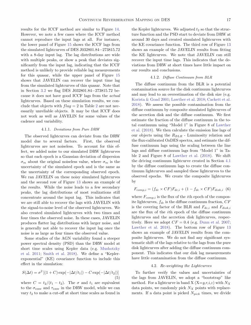
results for the ICCF method are similar to Figure 14.

However, we note a few cases where the ICCF method

cannot reproduce the input lags at all. For instance,

the lower panel of Figure 15 shows the ICCF lags from

the simulated lightcurves of DES J032801.84−273815.72

with a 8-day input lag. The lag distributions are wide

with multiple peaks, or show a peak that deviates sig-

nificantly from the input lag, indicating that the ICCF

method is unlikely to provide reliable lag measurements

for this quasar, while the upper panel of Figure 15

shows that JAVELIN can recover the input time lag

from the simulated lightcurves of this quasar. Note that

in Section 3.2 we flag DES J032801.84−273815.72 be-

cause it does not have good ICCF lags from the actual

lightcurves. Based on these simulation results, we con-

clude that objects with flag = 2 in Table 2 are not nec-

essarily unreliable objects. It may be that ICCF does

not work as well as JAVELIN for some values of the

cadence and variability.

4.1.1. Deviations from Pure DRW

The observed lightcurves can deviate from the DRW

model due to several factors. First, the observed

lightcurves are not noiseless. To account for this ef-

fect, we added noise to our simulated DRW lightcurves

so that each epoch is a Gaussian deviation of dispersion

σm about the original noiseless value, where σm is the

uncertainty of the simulated epoch and is the same as

the uncertainty of the corresponding observed epoch.

We ran JAVELIN on these noisy simulated lightcurves

and the second row of Figure 13 shows an example of

the results. While the noise leads to a few secondary

peaks, the lag distributions of most realizations still

concentrate around the input lag. This indicates that

we are still able to recover the lags with JAVELIN with

the signal-to-noise level of the observed lightcurves. We

also created simulated lightcurves with two times and

four times the observed noise. In these cases, JAVELIN

produces flatter lag distributions with larger noise, and

is generally not able to recover the input lag once the

noise is as large as four times the observed value.

Some studies of the AGN variability found a steeper

power spectral density (PSD) than the DRW model at

short time scales using Kepler data (e.g. Mushotzky

et al. 2011; Smith et al. 2018). We define a “Kepler-

exponential” (KE) covariance function to include this

effect in the simulation:

S(∆t) = σ2 [(1 + C) exp(−|∆t/t1|)− C exp(−|∆t/t2|)](5)

where C = t2/(t1 − t2). The σ and t1 are equivalent

to the σDRW and τDRW in the DRW model, while we can

vary t2 to make a cut-off at short time scales as found in

the Kepler lightcurves. We adjusted t2 so that the struc-

ture function and the PSD start to deviate from DRW at

around 30 days and created simulated lightcurves with

the KE covariance function. The third row of Figure 13

shows an example of the JAVELIN results from fitting

the KE lightcurves. We note that JAVELIN can still

recover the input time lags. This indicates that the de-

viations from DRW at short times have little impact on

our results and conclusions.

4.1.2. Diffuse Continuum from BLR

The diffuse continuum from the BLR is a potential

contamination source for the disk continuum lightcurves

and may lead to an overestimation of the disk size (e.g.

Korista & Goad 2001; Lawther et al. 2018; Cackett et al.

2018). We assess the possible contamination from the

diffuse continuum by composite simulated lightcurves of

the accretion disk and the diffuse continuum. We first

estimate the fraction of the diffuse continuum in the to-

tal continuum using “Model 1” in Figure 8 of Lawther

et al. (2018). We then calculate the emission line lags of

our objects using the RBLR - Luminosity relation and

the flux-calibrated OzDES spectra, and estimate the dif-

fuse continuum lags using the scaling between the line

lags and diffuse continuum lags from “Model 1” in Ta-

ble 2 and Figure 8 of Lawther et al. (2018). We shift

the driving continuum lightcurve created in Section 4.1

by the diffuse continuum lags to create the diffuse con-

tinuum lightcurves and sampled these lightcurves to the

observed epochs. We create the composite lightcurves

by

Fcomp,i = (fdc × CF )Fdc,i + (1− fdc × CF )Fdisk,i (6)

where Fcomp,i is the flux of the ith epoch of the compos-

ite lightcurves, fdc is the diffuse continuum fraction, CF

is the covering factor of the BLR and Fdc,i and Fdisk,iare the flux of the ith epoch of the diffuse continuum

lightcurves and the accretion disk lightcurves, respec-

tively. Here we adopt CF = 0.4 (e.g. Dunn et al. 2007;

Lawther et al. 2018). The bottom row of Figure 13

shows an example of JAVELIN results from the com-

posite lightcurves. We do not find any significant sys-

tematic shift of the lags relative to the lags from the pure

disk lightcurves after adding the diffuse continuum com-

ponent. This indicates that our disk lag measurements

have little contamination from the diffuse continuum.

4.2. Re-weighting the Lightcurves

To further verify the values and uncertainties of

the lags from JAVELIN, we adopt a “bootstrap” like

method. For a lightcurve in band X (X=g,r,i,z ) withNXdata points, we randomly pick NX points with replace-

ments. If a data point is picked Npick times, we divide

18 Yu et al.

0.0

0.5

1.0Pure DRWlag = 1 day(s) lag = 2 day(s) lag = 4 day(s) lag = 8 day(s)

0.0

0.5

1.0Noise addedlag = 1 day(s) lag = 2 day(s) lag = 4 day(s) lag = 8 day(s)

0.0

0.5

1.0Kepler-exponential lightcurveslag = 1 day(s) lag = 2 day(s) lag = 4 day(s) lag = 8 day(s)

−10 −5 0 5 100.0

0.5

1.0Disk+DClag = 1 day(s)

)10 )5 0 5 10

lag = 2 da((s)

)10 )5 0 5 10

lag = 4 da((s)

)10 )5 0 5 10 15

lag = 8 da((s)

lag(da(s, r band)

Figure 13. Probability distribution of r -band time lags relative to g-band from fitting the five realizations (LC0 - LC4) of the simulated

light curves of DES J063037.48−575610.30 in the MaxVis field. The histograms with different colors in each panel represent the JAVELIN

result for different realizations of the simulated lightcurves. The black dashed line in each panel represents the position of the input time

lag, which is 1, 2, 4 and 8 day(s) for the first, second, third and fourth column, respectively. The first through the fourth row represent

the results from pure DRW lightcurves, DRW lightcurves with noise, Kepler-exponential lightcurves and the composite lightcurves of the

accretion disk and the diffuse continuum from the BLR.

its errorbar by√Npick. If a data point is not picked, we

double its errorbar. We do not simply exclude the data

point like the traditional “bootstrap” method, since the

cadence is critical to the time series analysis, while in

the traditional “bootstrap” there is no equivalent to

the “time” axis for the lag measurements. Doubling

the errorbar significantly reduces the weight in the data

point, which does similar job as removing the data point

without qualitatively changing the lightcurve. We cre-

ated 80 re-weighted lightcurves for a few representative

objects in the main sample, and we ran JAVELIN on

each of the re-weighted lightcurves. We obtain the me-

dian JAVELIN lag of each re-weighted lightcurve, and

compare its distribution to the previous lag distribu-

tions from JAVELIN and ICCF. Figure 16 shows the

results of DES J063037.48−575610.30 from the MaxVis

field in the upper row and DES J034001.53−274036.91

from the C26202 fields in the lower row. The median

lag distributions from the re-weighted lightcurves are

generally consistent with the previous JAVELIN and

ICCF results. The z -band lag distribution of DES

J063037.48−575610.30 from the re-weighted lightcurves

show a small secondary peak near −5 days, possibly

due to the common ∼ 5-day gaps in its lightcurve. The

positive lag distributions are still consistent with previ-

Continuum Reverberation Mapping on DES 19

−10 −5 0 5 100.0

0.2

0.4

0.6

0.8lag = 1 day(s)

−10 −5 0 5 10

lag = 2 day(s)

−10 −5 0 5 10

lag = 4 day(s)

−10 0 10

lag = 8 day(s)

lag(days, r band)

Figure 14. Probability distribution of r -band time lags relative to g-band from fitting the five realizations (LC0 - LC4) of the simulated

DRW light curves with the same ∼ 1 day cadence as DES J063037.48−575610.30 (same quasar as Figure 13) with ICCF. The histograms

with different colors in each panel represent the ICCF center distributions for different realizations of the DRW lightcurves. The black

dashed line in each panel represents the position of the input time lag, which is 1, 2, 4 and 8 day(s) for the first, second, third and fourth

column, respectively.

0.0

0.1

0.2

0.3

0.4JAVELIN Results

−10 0 10 20 30lag(days, r band)

0.000

0.025

0.050

0.075

ICCF Results

N rm

alize

d Distrib

uti n

Figure 15. Probability distribution of r -band time lags rel-

ative to g-band from fitting the simulated DRW lightcurves of

DES J032801.84−273815.72 with JAVELIN (upper panel) and

ICCF(lower panel). The histograms with different colors in each

panel represent the JAVELIN or ICCF results for different real-

izations of the DRW lightcurves. The black dashed line in each

panel represents the position of the 8-day input time lag.

ous lag distributions. These results again verify our lag

measurements in Section 3.

4.3. “Gaussianity” of the Photometric Errors

One assumption of JAVELIN is that the input errors

are Gaussian. We therefore assess the “Gaussianity”

of the photometric errors from DES with the standard

stars in the SDSS Stripe 82 fields. We select a subsample

of the standard stars from the SDSS Stripe 82 standard

star catalog by Ivezic et al. (2007) with the same dis-

tribution of g-band magnitudes as the whole standard

star sample. We construct DES lightcurves for the stars

following the same process as our quasar sample, and

exclude the stars that have less than 200 epochs over

the five DES observational seasons or have unreliable

photometries based on DES flags. For each standard

star, we calculate the ratio (mi,X −mX)/σi,X for each

data point in the lightcurve, where mi,X and σi,X repre-

sents the magnitude and magnitude error of the ith data

point in band X (X=g,r,i,z,Y ), and mX represents the

mean magnitude in band X. Assuming that the standard

stars from Ivezic et al. (2007) are non-variable objects,

the distribution of the ratio (mi,X − mX)/σi,X should

follow a Gaussian distribution centered at 0 with a stan-

dard deviation equal to 1. In addition, we calculate χ2r

defined in Section 3 for the whole SV - Y3 period for

each standard star. If the photometric errors are well

estimated, χ2r should be close to 1. We do not include

the Y4 data in this section, since the calibrations for the

Y4 data in the MaxVis field and the SDSS fields differ

from the DES FGCM calibration (Burke et al. 2018) for

other seasons and fields, and none of the lag measure-

ments in the main sample are from the Y4 data in these

fields.

Figure 17 shows an example of the distribution of

(mi,X −mX)/σi,X for a standard star with χ2r around

20 Yu et al.

−5 0 50

1

2

3 DES J063037.48-575610.30JAVELINICCF(cent)ICCF(peak)Re-weight

−5 0 50

1

2

−5 0 50

2

4

−10 0 10lag(days, r band)

0.0

0.2

0.4DES J034001.53-274036.91

−10 0 10lag(days, i band)

0.0

0.2

0.4

0.6

.10 0 10lag(da,), − band)

0.0

0.2

0.4

0.6

Figure 16. Probability distribution of time lags in the r, i, z band relative to g band for DES J063037.48−575610.30 (upper row) and

DES J034001.53−274036.91(lower row). The blue solid, red dash-dotted and black dotted lines represent the results from JAVELIN, the

ICCF center distribution and the ICCF peak distribution, respectively. The green dashed line represents the distribution of the median

JAVELIN lags from fitting the re-weighted lightcurves.

1.05. The distribution agrees well with the superim-

posed Gaussian profile, indicating that the DES photo-

metric errors are consistent with Gaussian errors in this

case. Figure 18 shows χ2r of the standard stars as a func-

tion of the r -band magnitude in the upper panel, and

the distribution of the r -band magnitude of the main

quasar sample in the lower panel. Most stars within themagnitude range of most quasars in the main sample

show χ2r close to 1, indicating that the DES photomet-

ric errors for quasars within this magnitude range are

well estimated. We note that χ2r is also a good indicator

of “Gaussianity”, and most stars with χ2r close to 1 show

similar distributions as Figure 17, so we expect that

the DES photometric errors are also close to Gaussian

within the magnitude range of the main quasar sample.

For bright stars, χ2r becomes significantly larger than 1

if we do not consider the calibration errors, but stays

near 1 when we take the calibration errors into account.

This indicates that the total photometric uncertainties

of these bright stars are dominated by calibration errors.

Since the DES standard star observations generally fol-

low the same strategy among the fields we study, we

expect the results from the SDSS Stripe 82 fields are ap-

−6 −4 −2 0 2 4 6(mi,X−m)/σi,X

0.00

0.05

0.10

0.15

0.20

0.25

0.30

0.35

0.40

Norm

alize

d Distrib

ution

Reduced χ2 = 1.05r = 20.00 mag

Figure 17. Example of the “Gaussianity” of the DES pho-

tometric errors. The blue histograms show the distribution of

(mi,X − mX)/σi,X for a standard star. The red line shows a

Gaussian profile centered at 0 with a standard deviation equal to

1. The upper left corner shows χ2r value (see Section 4.3) and the

r -band magnitude of the star.

plicable to our other fields. We therefore conclude that

the photometric errors of the FGCM calibrated DES

data are Gaussian and of the correct amplitude.

Continuum Reverberation Mapping on DES 21

15 16 17 18 19 20 21 22

2

4

6

8

10

12

14

16Re

duce

d χ2

Standard stars With calibration errorsWithout calibration errors

15 16 17 18 19 20 21 22Magnitude (r band)

0

2

4

6

8

N

Quasars in the final sample

Figure 18. (upper panel) χ2r (see Section 4.3) as a function of

the r -band magnitude for the standard stars. The blue crosses

show χ2r where we do not consider the DES calibration errors,

while the red points represent the cases where we add the DES cali-

bration errors following the same process as the quasar lightcurves.

The black dashed line represents the position where χ2r equals 1.

(lower panel) Magnitude distribution of the quasars in the main

sample.

5. DISK SIZE - BLACK HOLE MASS RELATION

For objects within the MaxVis and the C26202 fields,

we estimate the SMBH mass of each quasar in the main

sample through the single-epoch method using the broad

Hβ, Mg II or C IV line in the OzDES spectra. We

calculate the black hole mass as

MBH = fRBLR∆V 2

G(7)

where RBLR is the size of BLR, ∆V is the line width of

the broad emission line used for the estimation, and f is

the dimensionless “virial factor” that accounts for other

unknown factors, such as the inclination, structure and

kinematics of the BLR.

We use the line dispersion of the broad emission lines

as our indicator of the line width, as previous studies

have shown this provides more robust black hole mass

estimates compared to the Full-Width Half Maximum

(FWHM) (e.g. Peterson et al. 2004). The line dispersion

is defined as

σ2line(λ) =

[∫λ2P (λ)dλ

/∫P (λ)dλ

]− P0(λ)2 (8)

where P (λ) is the line profile and P0(λ) is the first

moment of the line profile. We use the public code

PySpecKit (Ginsburg & Mirocha 2011) in the analy-

sis of the spectra. For the Mg II line, we also fit and

subtract the iron emission lines using the template from

Vestergaard & Wilkes (2001).

We measure the monochromatic luminosity using the

flux-calibrated OzDES spectra (Hoormann et al. 2019),

and calculate RBLR using the RBLR - Luminosity re-

lations from Bentz et al. (2013) for Hβ, from McLure

& Jarvis (2002) for Mg II and from Hoormann et al.

(2019) for C IV. We adopt a virial factor of f = 4.31

from Grier et al. (2013). For objects within the SDSS

fields, we adopt the single-epoch black hole masses from

Shen et al. (2011). The error in single epoch black hole

mass is roughly 0.4 dex, based on the uncertainties in

the virial factor and the RBLR - Luminosity relation

(e.g. Peterson 2014). We do not further consider the

uncertainties from the line width and continuum lumi-

nosity measurements for individual objects, which are

very small compared to 0.4 dex.

In comparison to the observed accretion disk sizes, the

disk sizes predicted by the standard thin disk model at

effective wavelength λ has the analytical form

Rλ =

[(GM

8πσ

)(LEddηc2

)(3 + κ)mE

]1/3(kλ

hc

)4/3

(9)

where M is the mass of the SMBH, LEdd is the Ed-

dington luminosity, mE is the Eddington ratio defined

as the bolometric luminosity LBol divided by the Ed-

dington luminosity, η is the radiative efficiency defined

as LBol = ηMc2, where M is the mass accretion rate,

and κ is the ratio of external to internal heating. Note

that the disk size in Equation (9) is defined as the po-

sition where kT (Rλ) = hc/λ. This in fact assumes that

the emission at wavelength λ is solely contributed from

radius R. However, in reality the emission at λ also has

contributions from other radii. The disk size from con-

tinuum reverberation mapping is in fact a flux-weighted

mean radius 〈Rλ〉 defined as

〈Rλ〉 =

∫∞Rmin

B(T (R))R2 dR∫∞Rmin

B(T (R))RdR= XRλ (10)

where Rmin is the inner edge of the disk and B(T ) is the

Planck function. Assuming the inner edge Rmin → 0,

the conversion factor X = 2.494/3 = 3.36 if the disk

emission does not vary. (e.g. Fausnaugh et al. 2016; Tie

& Kochanek 2018).

Tie & Kochanek (2018) found that the conversion fac-

tor X will be larger when taking the variation of the disk

emission into account. Assuming the “lamppost” model

(e.g. Cackett et al. 2007) for the variability, the temper-

ature fluctuation of the disk is

T (R, t) = T0(R)[1 + f(t−R/c)] (11)

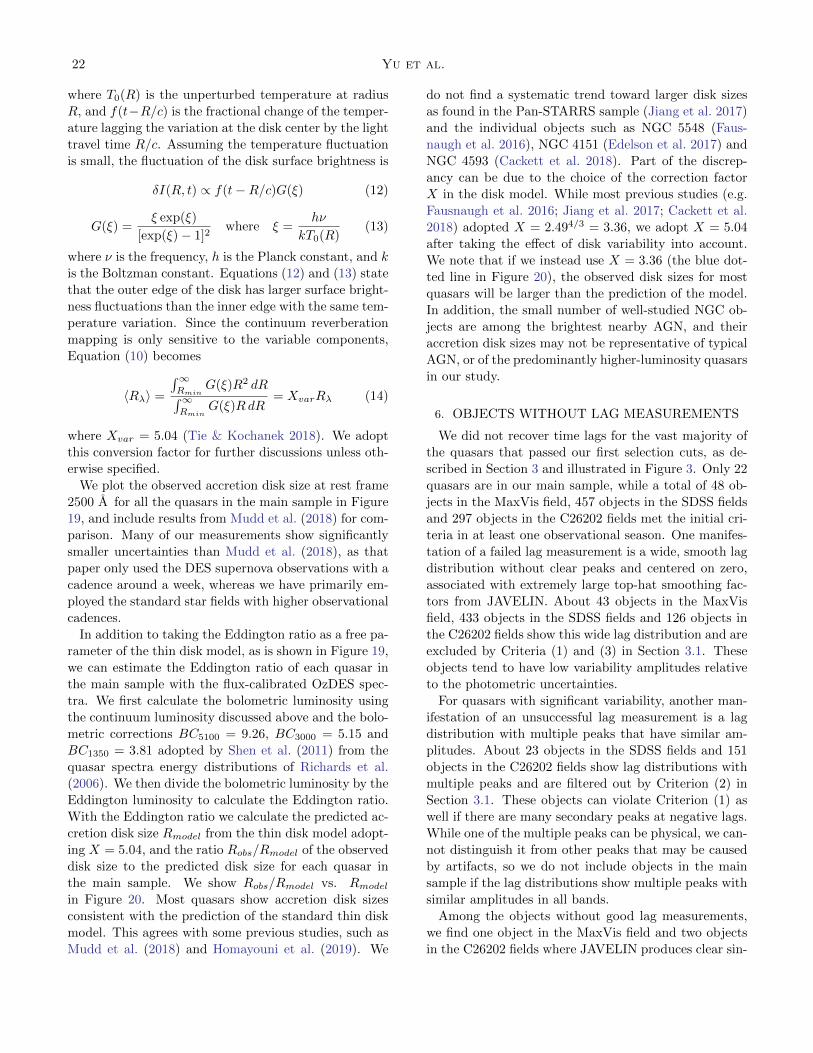
22 Yu et al.

where T0(R) is the unperturbed temperature at radius

R, and f(t−R/c) is the fractional change of the temper-

ature lagging the variation at the disk center by the light

travel time R/c. Assuming the temperature fluctuation

is small, the fluctuation of the disk surface brightness is

δI(R, t) ∝ f(t−R/c)G(ξ) (12)

G(ξ) =ξ exp(ξ)

[exp(ξ)− 1]2where ξ =

hν

kT0(R)(13)

where ν is the frequency, h is the Planck constant, and k

is the Boltzman constant. Equations (12) and (13) state

that the outer edge of the disk has larger surface bright-

ness fluctuations than the inner edge with the same tem-

perature variation. Since the continuum reverberation

mapping is only sensitive to the variable components,

Equation (10) becomes

〈Rλ〉 =

∫∞Rmin

G(ξ)R2 dR∫∞Rmin

G(ξ)RdR= XvarRλ (14)

where Xvar = 5.04 (Tie & Kochanek 2018). We adopt

this conversion factor for further discussions unless oth-

erwise specified.

We plot the observed accretion disk size at rest frame

2500 A for all the quasars in the main sample in Figure

19, and include results from Mudd et al. (2018) for com-

parison. Many of our measurements show significantly

smaller uncertainties than Mudd et al. (2018), as that

paper only used the DES supernova observations with a

cadence around a week, whereas we have primarily em-

ployed the standard star fields with higher observational

cadences.

In addition to taking the Eddington ratio as a free pa-

rameter of the thin disk model, as is shown in Figure 19,

we can estimate the Eddington ratio of each quasar in

the main sample with the flux-calibrated OzDES spec-

tra. We first calculate the bolometric luminosity using

the continuum luminosity discussed above and the bolo-

metric corrections BC5100 = 9.26, BC3000 = 5.15 and

BC1350 = 3.81 adopted by Shen et al. (2011) from the

quasar spectra energy distributions of Richards et al.

(2006). We then divide the bolometric luminosity by the

Eddington luminosity to calculate the Eddington ratio.

With the Eddington ratio we calculate the predicted ac-

cretion disk size Rmodel from the thin disk model adopt-

ing X = 5.04, and the ratio Robs/Rmodel of the observed

disk size to the predicted disk size for each quasar in

the main sample. We show Robs/Rmodel vs. Rmodelin Figure 20. Most quasars show accretion disk sizes

consistent with the prediction of the standard thin disk

model. This agrees with some previous studies, such as

Mudd et al. (2018) and Homayouni et al. (2019). We

do not find a systematic trend toward larger disk sizes

as found in the Pan-STARRS sample (Jiang et al. 2017)

and the individual objects such as NGC 5548 (Faus-

naugh et al. 2016), NGC 4151 (Edelson et al. 2017) and

NGC 4593 (Cackett et al. 2018). Part of the discrep-

ancy can be due to the choice of the correction factor

X in the disk model. While most previous studies (e.g.

Fausnaugh et al. 2016; Jiang et al. 2017; Cackett et al.

2018) adopted X = 2.494/3 = 3.36, we adopt X = 5.04

after taking the effect of disk variability into account.

We note that if we instead use X = 3.36 (the blue dot-

ted line in Figure 20), the observed disk sizes for most

quasars will be larger than the prediction of the model.

In addition, the small number of well-studied NGC ob-

jects are among the brightest nearby AGN, and their

accretion disk sizes may not be representative of typical

AGN, or of the predominantly higher-luminosity quasars

in our study.

6. OBJECTS WITHOUT LAG MEASUREMENTS

We did not recover time lags for the vast majority of

the quasars that passed our first selection cuts, as de-

scribed in Section 3 and illustrated in Figure 3. Only 22

quasars are in our main sample, while a total of 48 ob-

jects in the MaxVis field, 457 objects in the SDSS fields

and 297 objects in the C26202 fields met the initial cri-

teria in at least one observational season. One manifes-

tation of a failed lag measurement is a wide, smooth lag

distribution without clear peaks and centered on zero,

associated with extremely large top-hat smoothing fac-

tors from JAVELIN. About 43 objects in the MaxVis

field, 433 objects in the SDSS fields and 126 objects in

the C26202 fields show this wide lag distribution and are

excluded by Criteria (1) and (3) in Section 3.1. These

objects tend to have low variability amplitudes relative

to the photometric uncertainties.

For quasars with significant variability, another man-

ifestation of an unsuccessful lag measurement is a lag

distribution with multiple peaks that have similar am-

plitudes. About 23 objects in the SDSS fields and 151

objects in the C26202 fields show lag distributions with

multiple peaks and are filtered out by Criterion (2) in

Section 3.1. These objects can violate Criterion (1) as

well if there are many secondary peaks at negative lags.

While one of the multiple peaks can be physical, we can-

not distinguish it from other peaks that may be caused

by artifacts, so we do not include objects in the main

sample if the lag distributions show multiple peaks with

similar amplitudes in all bands.

Among the objects without good lag measurements,

we find one object in the MaxVis field and two objects

in the C26202 fields where JAVELIN produces clear sin-

Continuum Reverberation Mapping on DES 23

107 108 109

BH Mass (M⊙⊙

10−1

100

101

Disk

Size

a 2

500 Å

(l -day

s)

medd=0.1medd=0.3medd=1.0SDSS(Hβ)C26202(Hβ)C26202(MgII)C26202(CIV)MaxVis(Hβ)MaxVis(MgII)Mudd+17

Figure 19. Accretion disk size at rest frame 2500 A as a function of black hole mass. The blue dash-dotted, green dashed and red dotted

lines represent the prediction of the thin disk model for Eddington ratios of 0.1, 0.3 and 1.0, respectively. The red diamonds, blue squares,

black circles and cyan pentagons represent the results from the MaxVis field, the C26202 field, the SDSS fields and Mudd et al. (2018),

with errorbars for the 1σ uncertainties. For the objects from this work, the smaller markers with dashed errorbars represent the flagged

objects, while the larger markers with solid errorbars represent the objects with flag = 0 (the most secure results). The open hexagons

represent black hole masses measured from C IV. Other open markers represent black hole masses measured from Mg II, while the filled

markers represent black hole masses measured from Hβ. The typical uncertainty of the black hole mass is about 0.4 dex, shown as the

black errorbar in the bottom right corner.

gle peaks located at zero or negative lags. As an ex-

ample, the upper panel of Figure 21 shows the z -band

lag distribution from the observed lightcurves of DES

J063227.29−583915.00. The lag distribution peaks at

a negative lag, which is inconsistent with the standard

thin disk model. To verify whether the negative lags are

real, we perform simulations as described in Section 4.1

with 80 realizations. The lower panel of Figure 21 shows

the simulation results of DES J063227.29−583915.00 for

a simulated lag of 1 day, the predicted z -band lag from

the thin disk model for this object. The lag distribu-

tions from most realizations (∼ 64%) are smooth dis-

tributions without clear peaks. Only a small fraction

(∼ 36%) show very wide peaks around the input lag

with the peak probability density larger than 0.15, while

nearly none of the peaks are significant lag detections

according to the standards we used to generate our lag

measurements of the main sample in Section 3. This

indicates that we are unlikely to obtain a reliable lag

measurement for this object. We get similar results from

simulations of other objects that seem to have zero or

negative lag measurements, and we do not find any ob-

jects that show zero or negative lag that are verified by

simulations. Note that the number of clear positive lags

(22) is significantly larger than the number of possible

zero/negative lags we found (3), and none of the possi-

ble zero/negative lags are as significant as the positive

lags in the main sample. This indicates that the false

positive rate of our sample is very low.

In addition to quantifying the number of negative lags,

we also reversed the time order of our lightcurves to ver-

ify that reversing the time order produces negative lags.

This is to check that our lag detection algorithms are

not biased to yield positive measurements. We created

time-reversed lightcurves for all objects in the main sam-

ple in the seasons with lag measurements. For objects

with multi-season results, we performed the test on the

first season that produces lag measurements. We ran

JAVELIN on these time-reversed lightcurves. Figure 22

shows examples of the comparison between the origi-

nal and time-reversed results. The original and time-

24 Yu et al.

100 101

R2500,model (lt-days)0

1

2

3

4

5

R 250

0,ob

s / R

2500

,mod

el

SDSS (Hβ)C26202 (Hβ)C26202 (Mg II)C26202 (C IV)MaxVis (Hβ)MaxVis (Mg II)

Figure 20. Ratio Robs/Rmodel of the observed disk size to the predicted disk size vs. the thin disk model prediction. The symbols

have the same meaning as Figure 19. The red dashed line is drawn at Robs/Rmodel = 1 where the observed disk size equals the predicted

disk size from the model using X = 5.04. The blue dotted line is drawn at Robs/Rmodel = 0.67 where the observed disk size equals the

predicted disk size with X = 3.36. The uncertainty of the predicted accretion disk is shown as the black errorbar in the bottom right

corner, considering that the uncertainty of the black hole mass is about 0.4 dex.

reversed lightcurves produce nearly 1 symmetric distri-

butions about zero. That is, reversing the time sequence

simply changes the sign of the lags. In this case, the only

objects that will possibly have positive detections for the

time-reversed lightcurves are those with clear negative

lags. As discussed above, we only found 3 insignificant

zero/negative lags and therefore a very low false positive

rate.

7. EFFECT OF CADENCE ON LAG

MEASUREMENTS

The next generation large sky survey after DES is the

Large Synoptic Survey Telescope (LSST) project (e.g.

LSST Science Collaboration et al. 2009). LSST will

carry out a survey covering about 20000 deg2, repeatedly

scanning the region about 1000 times during a 10-year

period. In addition to the main survey, LSST plans to

intensively observe a set of Deep Drilling Fields (DDFs),

1 They are not exactly symmetric because of the random sam-pling inherent in the Markov Chain Monte Carlo method used byJAVELIN

with about 5% of the total observing time. Each DDF

has a diameter of 3.5 degrees, and the five DDFs in the

LSST Reference Simulated Survey “minion 1016” (e.g.

LSST Science Collaboration et al. 2017) cover about

50 deg2 in total. The large amount of observing time

dedicated in each Deep Drilling Field is likely to enable

the measurement of accretion disk sizes for many more

quasars and with smaller uncertainties. In this section,

we use our results to consider how to optimize the obser-

vation strategy for the DDFs to measure more accretion

disk sizes.

One of the most important factors that affect disk

size measurements is the observational cadence, which

is still under discussion for the LSST DDFs. We inves-

tigate the effect of observational cadence on the fraction

of quasars with good disk size measurements with simu-

lated lightcurves. To construct simulated lightcurves, we

first use the LSST Operation Simulator (OpSim) v3.3.5

(Delgado et al. 2014) to generate the observation sched-

ule, as well as the depth of each epoch. We use three

configurations in running OpSim. One is the official

configuration of the LSST Reference Simulated Survey

Continuum Reverberation Mapping on DES 25

Figure 21. (upper panel) Probability distribution of the

time lags in the z band from the observed lightcurves of DES

J063227.29−583915.00 from JAVELIN. (lower panel) z -band lag

distributions from 80 realizations of the simulated lightcurves of

DES J063227.29−583915.00 with an input time lag of 1 day. The

red dashed line shows the position of the input time lag. The

blue dotted line shows the position where the probability density

equals 0.15. Only 36% of the realizations show significant peaks

with the peak probability density larger than 0.15.

“minion 1016”. In this configuration, the Deep Drilling

Fields are observed on a roughly 3-day cadence in the

grizY bands. The mean 5σ depth in each epoch is about

25.02, 25.35, 24.81 and 24.48 mag for the g, r, i and zbands, respectively. We refer to this configuration as the

“3-day configuration”. We create the “2-day configura-

tion” and “1-day configuration” by requesting OpSim to

increase the number of epochs by a factor of 1.5 and 3,

respectively, while reducing the exposure time in each

single epoch such that the net integration time is nearly

unchanged. The “2-day configuration” has an observa-

tional cadence around 2 days, with a median 5σ depth

about 24.84, 25.13, 24.57 and 24.25 mag for the g, r,

i and z bands, respectively. The “1-day configuration”

has nearly daily observational cadence, with a median

5σ depth about 24.51, 24.73, 24.21 and 23.81 mag for

the g, r, i and z bands, respectively. The total exposure

time obtained in the Deep Drilling Fields for the three

configurations is nearly identical.

We then simulated a quasar with mean (g, r, i, z) =

(21.0, 20.5, 20.0, 19.5, 19.2) mag using a DRW. We con-

verted the magnitudes to fluxes with arbitrary units for

the lightcurves, and adopted DRW parameters σDRW =

2.5 (flux unit) and τDRW = 200 days. The mean magni-

tudes and DRW parameters are typical of the quasars

in our DES sample. We created the DRW lightcurves

following a similar procedure to what is described in Sec-

tion 4.1, and with the cadence specified by the observa-

tion schedule from OpSim. Combining the magnitude

of the quasar and the depth of LSST, we calculate the

photometric uncertainties in each epoch. To allow for

additional uncertainties, such as if the variability does

not exactly follow the DRW, or systematics in the mag-

nitude measurements in the single-epoch data, we set

the minimum uncertainty of each data point to be 1%,

even if all the photometric uncertainties are predicted

to be smaller.

Figure 23 shows an example of the three simulated

lightcurves in the g band in the left column. One fea-

ture of the observation schedules from OpSim is that the

lightcurves have gaps between a series of continuous ob-

servations, and the width of the gap is about a week. To

investigate the effect of these gaps on lag measurements,

we create another version of the simulated lightcurves

with the gaps removed. Specifically, if an observation is

more than 5 days away from the previous observation,

we change this observation to the date when it is 1 day,

2 days or 3 days after the previous observation, depend-

ing on the typical cadence of the lightcurve. As part of

this process, we reduce the length of the baseline, while

keeping the number of epochs constant. We show an

example of the lightcurves without gaps in the right col-

umn of Figure 23. These three alternate scenarios use

the same total integration time, although the removal of

the gaps decreases the total baseline of observations by

approximately a factor of 2.

For these six scenarios, i.e. 1-day, 2-day or 3-day ca-

dence, with or without gaps, we create 25 realizations

of the DRW lightcurves in the g band. We shift the

g-band lightcurves by the same input time lag in r, i

and z bands to create the simulated lightcurves in these

bands. The input time lag ranges from 1 day to 8 days

in steps of 1 day. We use JAVELIN to measure the

time lags between simulated lightcurves, and define a

successful measurement for one band if the JAVELIN

results satisfy:

1. The 1σ lower limit from the probability distribu-

tion of the time lag is larger than 0;

2. The lag distribution shows a clear single peak at

a positive lag; and

3. The 1σ upper limit of the top-hat smoothing factor

is smaller than 50.

26 Yu et al.

−5 0 50

1

2

3DES J063037.48-575610.30(SV)

O iginalReve sed

−5 0 50

1

2

−5 0 50

2

4

−5 0 5lag(days, band)

0.0

0.2

0.4DES J034001.53-274036.91(Y1)

−5 0 5lag(days, i band)

0.0

0.2

0.4

−5 0 5lag(days, z band)

0.0

0.2

0.4

0.6

Figure 22. Time lag distributions from JAVELIN for the time-reversed lightcurves in comparison with the original lightcurves. The

upper and lower row show the results for DES J063037.48−575610.30 and DES J034001.53−274036.91, respectively. The first through

the third column give the time lag distributions in the riz bands, respectively. The blue solid lines represents the results for the original

lightcurves, while the red dashed lines are for time-reversed lightcurves. See Section 6 for more details.

We added the third criterion because large smoothing

factors are usually associated with smooth lag distribu-

tions without clear peaks, which is a common feature of

the failed fits from JAVELIN. We define a successful lag

recovery for a realization if the time lags are successfully

measured in at least two of the r, i and z bands. We

define the lag recovery fraction as the number of realiza-

tions where we recover lags successfully divided by the

total number of realizations (25). We plot the recovery

fraction as a function of input time lag in Figure 24. For

input times lags smaller than 5 days, the lag recovery

fractions increase significantly toward higher cadences.

Notably, for an input lag of one day, the 2-day cadence

and 1-day cadence can increase the lag recovery frac-

tion by a factor up to 5 and 10 compared to the 3-day

cadence, respectively. For input time lags larger than

5 days, the trend can reverse for lightcurves with gaps,

which may be due to aliasing produced by the gaps in

the light curves. For lightcurves without gaps, higher

cadences never produce recovery fractions smaller than

those from lower cadences, as expected. This indicates

that we can significantly improve the yield of accretion

disk size measurements if we change the observational

cadence in the DDFs from the official 3 days to 2 days

or 1 day, while the total exposure time and the final

coadded depth of the DDFs will not be affected.

To estimate the distribution of the observed time lags

from real quasars, we use the SDSS DR7 quasar sam-

ple presented by Shen et al. (2011). The uniformly se-

lected quasar sample contains 59514 quasars with flux

limits of i = 19.1 mag at z < 2.9 and i = 20.2 mag at

z > 2.9, where i is the i -band magnitude and z is red-

shift. We adopt the fiducial single-epoch black hole mass

from Shen et al. (2011), and use the standard thin disk

model to calculate the accretion disk size and the time

lag in the r, i, and z band relative to g band assum-

ing the Eddington ratio equals 0.1. The lower panel in

Figure 24 shows the distribution of the predicted time

lag. A large fraction of the lags are less than 5 days,

where higher observational cadence can significantly in-

crease the recovery fraction. The observations of the

LSST DDFs will be much deeper than SDSS, and will

detect more low luminosity AGNs with smaller black

hole masses and hence smaller continuum lags. In ad-

dition, AGNs with smaller black hole masses tend to

be more variable and thus lag measurements should be

easier. We therefore expect more small time lags in the

LSST DDFs than what is implied by the lower panel in

Figure 24. Given that the observed continuum lags from

Continuum Reverberation Mapping on DES 27

real quasars are expected to be small, a higher observa-

tional cadence in the LSST DDFs can help improve the

yield of quasar accretion disk sizes significantly.

We present an order-of-magnitude estimate of the

number of successful continuum lag measurements in the

LSST DDFs. We relate the number of lag measurements

in the LSST DDFs to our DES results as

Nlags(< mlsst) = flsst ×Nqso(< mlsst) (15)

flsst =Σlags(< mdes)

Σqso(< mdes)× αcad × βdepth (16)

where Nlags,lsst is the total number of AGNs with con-

tinuum lag measurements in the LSST DDFs, Σlags(<

mdes) is the surface density of lag measurements in the

DES fields, Σqso(< mdes) of the surface density of AGNs

detected in the DES fields, Nqso(< mlsst) is the num-

ber of AGNs brighter than the magnitude limit mlsst

in the LSST DDFs, αcad is the correction factor of dif-

ferent cadences between DES and LSST, and βdepth is

the correction factor of different depths. We define the

magnitude limit mlsst as the magnitude corresponding

to 1% photometric errors and do not consider fainter

objects.

The term Σlags(< mdes)/Σqso(< mdes) represents the

fraction of continuum lag measurements in the DES

fields. We estimate this fraction based on the results

from the C26202 fields, which combine the 1-day cadence

standard star observations and 7-day cadence supernova

observations. We obtain 17 good measurements out

of 318 input AGNs, so we have Σlags(< mdes)/Σqso(<

mdes) ≈ 17/318 ≈ 0.0536.

We estimate the cadence correction factor αcad with

the same simulation framework as discussed above. The

mean observational cadence of the input quasar sample

in the C26202 fields is around 5 days, while the proposedcadence for AGN science in the LSST DDFs is around 2

days (Brandt et al. 2018). The mean continuum lag of

the riz bands relative to the g band in the C26202 fields

is around 3 days. We find that for an input time lag

of 3 days, a 2-day cadence can increase the lag recovery

fraction by a factor of about 1.35 compared to a 5-day

cadence, so we have αcad ≈ 1.35.

The correction factor βdepth accounts for the depth

difference between DES and LSST. One important dif-

ference is that deeper observations lead to smaller single-

epoch uncertainties. However, for the deep DES super-

nova and the LSST DDF observations, the single-epoch

uncertainties are dominated by calibration uncertainties

instead of statistical errors, so the improvement of lag

measurements from smaller single-epoch errors will not

be significant. Another difference is that deeper LSST

observations allows the detection of more low-luminosity

AGNs, which tend to be more variable and therefore

easier to measure lags. We note that the fraction of

successful measurements does increase toward lower lu-

minosities for our results from the C26202 fields, and we

estimate βdepth ≈ 2.32.

According to the LSST OpSim, the median single-

epoch 5σ depth in the i band for a 2-day cadence is

about 24.57 mag, so we have mi,lsst ≈ 23.8. Based on

the quasar luminosity functions by Manti et al. (2017),

we estimate log(Nqso) ≈ 4.2. Plugging these parame-

ters to Equation (15), we get Nlags(< mlsst) ≈ 2653.

That is, we expect to have about three thousand disk

size measurements in the LSST DDFs with a 2-day ob-

servation cadence.

We stress that this calculation is just an order-of-

magnitude estimate. Some potentially important effects

that we did not include are: (1) We did not consider

AGN with photometric errors larger than about 1%,

while these objects may also yield lag measurements.

(2) The fraction of lag measurements based on our DES

sample is limited by small number statistics. (3) When

estimating αcad and βdepth, we used the mean cadences,

lags and depths without considering the distribution of

these parameters in detail.

8. SUMMARY

We present quasar accretion disk size measurements

through continuum reverberation mapping using data

from DES standard star observations. We select spec-

troscopically confirmed as well as color and variability

selected quasars in the MaxVis field, the SDSS fields and

the C26202 fields, and construct continuum lightcurves

with the DES photometry from SV to Y4 in the griz

bands. We use the JAVELIN and ICCF methods to

measure time lags between different bands, and use

the JAVELIN Thin Disk model to fit for the accre-

tion disk sizes. We create simulated lightcurves and

re-weighted lightcurves to verify the lag measurements

from JAVELIN and ICCF. We confirm that the DES

photometric errors are Gaussian and appropriate for

JAVELIN. We also create simulated lightcurves in the

LSST DDFs, and probe the effect of observational ca-

dence on continuum lag measurements. Our main re-

sults are:

1. We successfully measure the time lags and accre-

tion disk sizes from 22 quasars, with black hole

mass spanning 107 - 109M, among which 17

have no flags and therefore are the most secure.

Our measurements have smaller uncertainties than

Mudd et al. (2018) thanks to the higher observa-

tional cadence of the DES standard star fields.

28 Yu et al.

10

15

20 3-day cadence, with gaps (23 epochs) 3-day cadence, without gaps (23 epochs)

10

15

20 2-day cadence, with gaps (31 epochs) 2-day cadence, without gaps (31 epochs)

3750 3800 3850 3900

10

15

20 1-day cadence, with gaps (54 epochs)

3750 3800 3850 3900

1-day cadence, without gaps (54 epochs)

MJD-56000

Flux

(g b

and)

Figure 23. Simulated g-band lightcurves for one observational season for quasars in the LSST DDFs. The fluxes are in arbitrary units.

The upper, middle and lower row show the lightcurve from a 3-day, 2-day and 1-day cadence from OpSim, respectively. The left column

shows the lightcurves with gaps, while the right column shows the lightcurves where gaps are removed. The lightcurves with the 3-day,

2-day and 1-day cadence have about 23, 31 and 54 epochs in one observational season, respectively.

2. Most of the measured accretion disk sizes are con-

sistent with the predictions of the standard thin

disk model if we take the disk variability into ac-

count.

3. We have simulated several alternative observation

strategies for the LSST DDFs and found that the

yield of accretion disk size measurements should

increase significantly if the cadence were changed

from 3 days to 2 days or 1 day.

We thank the anonymous referee for a thorough and

thoughtful report. This material is based upon work

supported by the National Science Foundation under

Grant No. 1615553. This research was funded partially

by the Australian Government through the Australian

Research Council through project DP160100930. Fund-

ing for the DES Projects has been provided by the U.S.

Department of Energy, the U.S. National Science Foun-

dation, the Ministry of Science and Education of Spain,

the Science and Technology Facilities Council of the

United Kingdom, the Higher Education Funding Coun-

cil for England, the National Center for Supercomput-

ing Applications at the University of Illinois at Urbana-

Champaign, the Kavli Institute of Cosmological Physics

at the University of Chicago, the Center for Cosmology

and Astro-Particle Physics at the Ohio State University,

Continuum Reverberation Mapping on DES 29

0 1 2 3 4 5 6 7 8

0.2

0.4

0.6

0.8

1.0

1.2

Recovery Fraction

LSST DDF Simulation 1-day2-day3-day

0 1 2 3 4 5 6 7 8lag (days)

0.0

0.1

0.2

SDSS DR7 QSO r bandi bandz band

Figure 24. (upper panel) Recovery fraction of time lags from

simulated lightcurves in the LSST DDFs as a function of input

time lags. The red squares, green diamonds and blue circles rep-

resent the result for lightcurves with a 1-day, 2-day and 3-day

cadence, respectively. The open symbols represent results from

lightcurves with gaps, while filled markers are from lightcurves

without gaps. (lower panel) Predicted lag distributions for the

SDSS DR7 quasars. The red, blue and black lines represents the

lag distribution in the r, i and z band relative to g band, respec-

tively.

the Mitchell Institute for Fundamental Physics and As-

tronomy at Texas A&M University, Financiadora de Es-

tudos e Projetos, Fundacao Carlos Chagas Filho de Am-

paro a Pesquisa do Estado do Rio de Janeiro, Conselho

Nacional de Desenvolvimento Cientıfico e Tecnologico

and the Ministerio da Ciencia, Tecnologia e Inovacao,

the Deutsche Forschungsgemeinschaft and the Collabo-

rating Institutions in the Dark Energy Survey.

The Collaborating Institutions are Argonne National

Laboratory, the University of California at Santa Cruz,

the University of Cambridge, Centro de Investigaciones

Energeticas, Medioambientales y Tecnologicas-Madrid,

the University of Chicago, University College Lon-

don, the DES-Brazil Consortium, the University of

Edinburgh, the Eidgenossische Technische Hochschule

(ETH) Zurich, Fermi National Accelerator Laboratory,

the University of Illinois at Urbana-Champaign, the

Institut de Ciencies de l’Espai (IEEC/CSIC), the In-

stitut de Fısica d’Altes Energies, Lawrence Berkeley

National Laboratory, the Ludwig-Maximilians Univer-

sitat Munchen and the associated Excellence Cluster

Universe, the University of Michigan, the National Op-

tical Astronomy Observatory, the University of Not-

tingham, The Ohio State University, the University of

Pennsylvania, the University of Portsmouth, SLAC Na-

tional Accelerator Laboratory, Stanford University, the

University of Sussex, Texas A&M University, and the

OzDES Membership Consortium.

Based in part on observations at Cerro Tololo Inter-

American Observatory, National Optical Astronomy

Observatory, which is operated by the Association of

Universities for Research in Astronomy (AURA) un-

der a cooperative agreement with the National Science

Foundation.

The DES data management system is supported by

the National Science Foundation under Grant Num-

bers AST-1138766 and AST-1536171. The DES par-

ticipants from Spanish institutions are partially sup-

ported by MINECO under grants AYA2015-71825,

ESP2015-66861, FPA2015-68048, SEV-2016-0588, SEV-

2016-0597, and MDM-2015-0509, some of which include

ERDF funds from the European Union. IFAE is par-

tially funded by the CERCA program of the Generali-

tat de Catalunya. Research leading to these results has

received funding from the European Research Coun-

cil under the European Union’s Seventh Framework

Program (FP7/2007-2013) including ERC grant agree-

ments 240672, 291329, and 306478. We acknowledge

support from the Australian Research Council Centre

of Excellence for All-sky Astrophysics (CAASTRO),

through project number CE110001020, and the Brazil-

ian Instituto Nacional de Ciencia e Tecnologia (INCT)

e-Universe (CNPq grant 465376/2014-2).

This manuscript has been authored by Fermi Re-

search Alliance, LLC under Contract No. DE-AC02-07CH11359 with the U.S. Department of Energy, Office

of Science, Office of High Energy Physics. The United

States Government retains and the publisher, by ac-

cepting the article for publication, acknowledges that

the United States Government retains a non-exclusive,

paid-up, irrevocable, world-wide license to publish or re-

produce the published form of this manuscript, or allow

others to do so, for United States Government purposes.

Software: JAVELIN (Zu et al. 2011), JAVELIN Thin

Disk Model (Mudd et al. 2018), PyCCF (Sun et al. 2018),

pyspeckit (Ginsburg & Mirocha 2011), Astropy (Astropy

Collaboration et al. 2013, 2018), SciPy (Jones et al. 2001),

Numpy(TravisE2006),Matplotlib(Hunter2007),Pandas

(McKinney 2010).

30 Yu et al.

APPENDIX

A. COMMENTS ON INDIVIDUAL LAG MEASUREMENTS

We comment on the time lag distributions in Figures 5 - 8 and discuss the comparisons between the JAVELIN and

ICCF results for each object in the main sample. First, we clarify the “consistency” between the two methods. There

are three cases:

(1) The lag distributions from both methods show clear peaks, and they agree with each other at the 1σ level.

(2) Only one method gives lag measurements, while the other method fails to measure the lags. This may also include

the case where the lag distribution does show a peak but is much wider than the distribution from the other method.

(3) The lag distributions from both methods show clear peaks, but they disagree with each other.

We add flag = 2 to the objects where JAVELIN and ICCF produce inconsistent lag distributions that satisfy (2) or

(3) in all bands.

While both (2) and (3) are cases of “inconsistent” results, case (2) is less critical since it only indicates that the

uncertainty estimates from the two methods are quite different, or one method does not work well for a particular

sampling of the lightcurve. This difference between JAVELIN and ICCF has been discussed in many RM studies

either on continuum or on emission lines (e.g. Grier et al. 2017; Mudd et al. 2018; Czerny et al. 2019), and detailed

studies on this difference are out of the scope of this paper.

Comments on the unflagged objects are as follows:

DES J063037.48-575610.30: The ICCF peak distribution in the i band shows a peak around 2.5 days, consistent

with the JAVELIN lag distributions. The ICCF center distributions are much wider than JAVELIN. This is in fact an

extreme case of the lag uncertainty difference between JAVELIN and ICCF. The ICCF center distributions do show

peaks and are consistent with JAVELIN at the 1σ level, while these peaks are too wide to see clearly in normalized

histogram plots.

DES J063510.91-585303.70: The ICCF distributions show clear peaks in all three bands and are consistent with

JAVELIN.

DES J063159.74-590900.60: The ICCF distributions show clear peaks in all three bands. The distributions are

consistent with JAVELIN in the i band and z band. The main peaks of ICCF in the r band differ slightly from the

JAVELIN results, but they still agree at the 1σ level.

DES J034003.89-264524.52: The ICCF distributions show clear peaks in all three bands and are consistent with

JAVELIN.

DES J032724.94-274202.81: The ICCF center distributions are much wider than JAVELIN in the r band and

i band, i.e., the case (2) discussed above. The ICCF center distribution in the z band shows a peak at negative lags

and disagree with the JAVELIN results. However, the ICCF peak distributions show clear peaks in all three bands

and are consistent with JAVELIN.

DES J033545.58-293216.51: The ICCF center distributions are generally much wider than JAVELIN. However,

the ICCF peak distributions show clear peaks in all three bands and are consistent with JAVELIN.

DES J033810.61-264325.00: The ICCF distributions show clear peaks in all three bands. They are consistent

with JAVELIN in the r band and i band. The JAVELIN results differ from the ICCF center distribution but still

agree with the ICCF peak distribution at the 1σ level in the z band.

DES J034001.53-274036.91: The ICCF distributions show clear peaks in all three bands and are consistent with

JAVELIN.

DES J033853.20-261454.82: The ICCF distributions show clear peaks in the r band, and are consistent with

JAVELIN. In the i band the ICCF distributions are much wider than JAVELIN and are closer to the case (2) discussed

above. The ICCF center distribution in the z band is ambiguous, while the ICCF peak distribution still shows a clear

peak and is consistent with JAVELIN.

DES J033051.45-271254.90: The ICCF distributions are ambiguous in the r band and z band, which satisfies

the case (2) inconsistency. However, the ICCF distribution in the i band shows a clear peak and is consistent with

JAVELIN.

DES J032853.99-281706.90: The ICCF center distributions are generally much wider than JAVELIN. However,

the ICCF peak distributions show clear peaks in all three bands and are consistent with JAVELIN in the i band and

z band. The ICCF peak distributions differ from JAVELIN in the r band.

Continuum Reverberation Mapping on DES 31

DES J033230.63-284750.39: The ICCF distributions show clear peaks in all three bands and are consistent with

JAVELIN.

DES J033729.20-294917.51: The ICCF distributions show clear peaks and are consistent with JAVELIN in the

r band. While the ICCF peak distributions are ambiguous in the i band, the ICCF center distributions still show a

peak and are consistent with JAVELIN at the 1σ level.

DES J033220.03-285343.40: The ICCF distributions show clear peaks in all three bands and are consistent with

JAVELIN in the i band and z band. While the ICCF peak distributions seem to differ from JAVELIN in the r band,

they still agree at the 1σ level.

DES J033342.30-285955.72: The ICCF distributions show clear peaks in all three bands and are consistent with

JAVELIN, except a slight difference between JAVELIN and the ICCF center distributions in the i band.

DES J033052.19-274926.80: The ICCF distributions show clear peaks in both bands and are consistent with

JAVELIN.

DES J033238.11-273945.11: The ICCF distributions are ambiguous in the r band and z band, which satisfies

the case (2) inconsistency. However, the ICCF results show clear peaks in the i band and are consistent with JAVELIN.

Comments on the flagged objects are as follows:

DES J062758.99-582929.60: The ICCF distributions are generally ambiguous and satisfy the case (2) inconsis-

tency with JAVELIN.

DES J033002.93-273248.30: The ICCF distributions are generally ambiguous and satisfy the case (2) inconsis-

tency with JAVELIN.

DES J033408.25-274337.81: The ICCF distribution are generally much wider than JAVELIN and are closer to

the case (2) inconsistency.

DES J032801.84-273815.72: The ICCF distributions are generally ambiguous and satisfy the case (2) inconsis-

tency with JAVELIN.

DES J005905.51+000651.66: The ICCF distributions are much wider than JAVELIN and are closer to the case

(2) inconsistency in the r band and z band. The ICCF distributions show clear peaks in the i band but disagree with

JAVELIN.

In summary, all unflagged objects in the main sample have consistent JAVELIN and ICCF results in at least one of

the riz bands. Most discrepancies between JAVELIN and ICCF follow the case (2) discussed above, and the case (3)

discrepancies are rare.

REFERENCES

Abbott, T. M. C., Abdalla, F. B., Allam, S., et al. 2018,

ApJS, 239, 18, doi: 10.3847/1538-4365/aae9f0

Adelman-McCarthy, J. K., Agueros, M. A., Allam, S. S.,

et al. 2007, ApJS, 172, 634, doi: 10.1086/518864

Astropy Collaboration, Robitaille, T. P., Tollerud, E. J.,

et al. 2013, A&A, 558, A33,

doi: 10.1051/0004-6361/201322068

Astropy Collaboration, Price-Whelan, A. M., Sipocz, B. M.,

et al. 2018, AJ, 156, 123, doi: 10.3847/1538-3881/aabc4f

Bentz, M. C., Denney, K. D., Grier, C. J., et al. 2013, ApJ,

767, 149, doi: 10.1088/0004-637X/767/2/149

Brandt, W. N., Ni, Q., Yang, G., et al. 2018, arXiv e-prints.

https://arxiv.org/abs/1811.06542

Burke, D. L., Rykoff, E. S., Allam, S., et al. 2018, AJ, 155,

41, doi: 10.3847/1538-3881/aa9f22

Cackett, E. M., Chiang, C.-Y., McHardy, I., et al. 2018,

ApJ, 857, 53, doi: 10.3847/1538-4357/aab4f7

Cackett, E. M., Horne, K., & Winkler, H. 2007, MNRAS,

380, 669, doi: 10.1111/j.1365-2966.2007.12098.x

Childress, M. J., Lidman, C., Davis, T. M., et al. 2017,

MNRAS, 472, 273, doi: 10.1093/mnras/stx1872

Collier, S. J., Horne, K., Kaspi, S., et al. 1998, ApJ, 500,

162, doi: 10.1086/305720

Czerny, B., Olejak, A., Ra lowski, M., et al. 2019, ApJ, 880,

46, doi: 10.3847/1538-4357/ab2913

Delgado, F., Saha, A., Chandrasekharan, S., et al. 2014, in

Proc. SPIE, Vol. 9150, Modeling, Systems Engineering,

and Project Management for Astronomy VI, 915015

Dexter, J., & Agol, E. 2011, ApJL, 727, L24,

doi: 10.1088/2041-8205/727/1/L24

32 Yu et al.

Dunn, J. P., Crenshaw, D. M., Kraemer, S. B., & Gabel,

J. R. 2007, AJ, 134, 1061, doi: 10.1086/520644

Edelson, R., Gelbord, J. M., Horne, K., et al. 2015, ApJ,

806, 129, doi: 10.1088/0004-637X/806/1/129

Edelson, R., Gelbord, J., Cackett, E., et al. 2017, ApJ, 840,

41, doi: 10.3847/1538-4357/aa6890

Fausnaugh, M. M., Denney, K. D., Barth, A. J., et al. 2016,

ApJ, 821, 56, doi: 10.3847/0004-637X/821/1/56

Fausnaugh, M. M., Starkey, D. A., Horne, K., et al. 2018,

ApJ, 854, 107, doi: 10.3847/1538-4357/aaaa2b

Flaugher, B., Diehl, H. T., Honscheid, K., et al. 2015, AJ,

150, 150, doi: 10.1088/0004-6256/150/5/150

Gaskell, C. M. 2017, MNRAS, 467, 226,

doi: 10.1093/mnras/stx094

Ginsburg, A., & Mirocha, J. 2011, PySpecKit: Python

Spectroscopic Toolkit, Astrophysics Source Code Library.

http://ascl.net/1109.001

Grier, C. J., Martini, P., Watson, L. C., et al. 2013, ApJ,

773, 90, doi: 10.1088/0004-637X/773/2/90

Grier, C. J., Trump, J. R., Shen, Y., et al. 2017, ApJ, 851,

21, doi: 10.3847/1538-4357/aa98dc

Haardt, F., & Maraschi, L. 1991, ApJL, 380, L51,

doi: 10.1086/186171

Hall, P. B., Sarrouh, G. T., & Horne, K. 2018, ApJ, 854,

93, doi: 10.3847/1538-4357/aaa768

Homayouni, Y., Trump, J. R., Grier, C. J., et al. 2019,

ApJ, 880, 126, doi: 10.3847/1538-4357/ab2638

Hoormann, J. K., Martini, P., Davis, T. M., et al. 2019,

MNRAS, 487, 3650, doi: 10.1093/mnras/stz1539

Hunter, J. D. 2007, Computing in Science & Engineering, 9,

90, doi: 10.1109/MCSE.2007.55

Ivezic, Z., Smith, J. A., Miknaitis, G., et al. 2007, AJ, 134,

973, doi: 10.1086/519976

Jiang, Y.-F., Green, P. J., Greene, J. E., et al. 2017, ApJ,

836, 186, doi: 10.3847/1538-4357/aa5b91

Jones, E., Oliphant, T., Peterson, P., et al. 2001, SciPy:

Open source scientific tools for Python.

http://www.scipy.org/

Kelly, B. C., Bechtold, J., & Siemiginowska, A. 2009, ApJ,

698, 895, doi: 10.1088/0004-637X/698/1/895

Korista, K. T., & Goad, M. R. 2001, ApJ, 553, 695,

doi: 10.1086/320964

Koz lowski, S., Kochanek, C. S., Udalski, A., et al. 2010,

ApJ, 708, 927, doi: 10.1088/0004-637X/708/2/927

Lawther, D., Goad, M. R., Korista, K. T., Ulrich, O., &

Vestergaard, M. 2018, MNRAS, 481, 533,

doi: 10.1093/mnras/sty2242

Li, Y.-P., Yuan, F., & Dai, X. 2019, MNRAS, 483, 2275,

doi: 10.1093/mnras/sty3245

LSST Science Collaboration, Abell, P. A., Allison, J., et al.

2009, ArXiv e-prints. https://arxiv.org/abs/0912.0201

LSST Science Collaboration, Marshall, P., Anguita, T.,

et al. 2017, ArXiv e-prints.

https://arxiv.org/abs/1708.04058

MacLeod, C. L., Ivezic, Z., Kochanek, C. S., et al. 2010,

ApJ, 721, 1014, doi: 10.1088/0004-637X/721/2/1014

Manti, S., Gallerani, S., Ferrara, A., Greig, B., & Feruglio,

C. 2017, MNRAS, 466, 1160, doi: 10.1093/mnras/stw3168

McHardy, I. M., Connolly, S. D., Horne, K., et al. 2018,

MNRAS, 480, 2881, doi: 10.1093/mnras/sty1983

McKinney, W. 2010, in Proceedings of the 9th Python in

Science Conference, ed. S. van der Walt & J. Millman, 51

– 56

McLure, R. J., & Jarvis, M. J. 2002, MNRAS, 337, 109,

doi: 10.1046/j.1365-8711.2002.05871.x

Morgan, C. W., Kochanek, C. S., Morgan, N. D., & Falco,

E. E. 2010, ApJ, 712, 1129,

doi: 10.1088/0004-637X/712/2/1129

Mudd, D., Martini, P., Zu, Y., et al. 2018, ApJ, 862, 123,

doi: 10.3847/1538-4357/aac9bb

Mushotzky, R. F., Edelson, R., Baumgartner, W., &

Gandhi, P. 2011, ApJL, 743, L12,

doi: 10.1088/2041-8205/743/1/L12

Peters, C. M., Richards, G. T., Myers, A. D., et al. 2015,

ApJ, 811, 95, doi: 10.1088/0004-637X/811/2/95

Peterson, B. M. 2014, SSRv, 183, 253,

doi: 10.1007/s11214-013-9987-4

Peterson, B. M., Wanders, I., Horne, K., et al. 1998, PASP,

110, 660, doi: 10.1086/316177

Peterson, B. M., Ferrarese, L., Gilbert, K. M., et al. 2004,

ApJ, 613, 682, doi: 10.1086/423269

Richards, G. T., Lacy, M., Storrie-Lombardi, L. J., et al.

2006, ApJS, 166, 470, doi: 10.1086/506525

Sergeev, S. G., Doroshenko, V. T., Golubinskiy, Y. V.,

Merkulova, N. I., & Sergeeva, E. A. 2005, ApJ, 622, 129,

doi: 10.1086/427820

Shakura, N. I., & Sunyaev, R. A. 1973, A&A, 24, 337

Shappee, B. J., Prieto, J. L., Grupe, D., et al. 2014, ApJ,

788, 48, doi: 10.1088/0004-637X/788/1/48

Shen, Y., Richards, G. T., Strauss, M. A., et al. 2011,

ApJS, 194, 45, doi: 10.1088/0067-0049/194/2/45

Shields, G. A. 1978, Nature, 272, 706,

doi: 10.1038/272706a0

Smith, K. L., Mushotzky, R. F., Boyd, P. T., et al. 2018,

ApJ, 857, 141, doi: 10.3847/1538-4357/aab88d

Sun, M., Grier, C. J., & Peterson, B. M. 2018, PyCCF:

Python Cross Correlation Function for reverberation

mapping studies, Astrophysics Source Code Library.

http://ascl.net/1805.032

Continuum Reverberation Mapping on DES 33

Sun, M., Xue, Y., Trump, J. R., & Gu, W.-M. 2019,

MNRAS, 482, 2788, doi: 10.1093/mnras/sty2885

Tie, S. S., & Kochanek, C. S. 2018, MNRAS, 473, 80,

doi: 10.1093/mnras/stx2348

Tie, S. S., Martini, P., Mudd, D., et al. 2017, AJ, 153, 107,

doi: 10.3847/1538-3881/aa5b8d

Travis E, O. 2006, A guide to NumPy.

http://www.numpy.org/

Vestergaard, M., & Wilkes, B. J. 2001, ApJS, 134, 1,

doi: 10.1086/320357

Wanders, I., Peterson, B. M., Alloin, D., et al. 1997, ApJS,

113, 69, doi: 10.1086/313054

Yuan, F., Lidman, C., Davis, T. M., et al. 2015, MNRAS,

452, 3047, doi: 10.1093/mnras/stv1507

Zu, Y., Kochanek, C. S., Koz lowski, S., & Udalski, A. 2013,

ApJ, 765, 106, doi: 10.1088/0004-637X/765/2/106

Zu, Y., Kochanek, C. S., & Peterson, B. M. 2011, ApJ, 735,

80, doi: 10.1088/0004-637X/735/2/80