Quasi-likelihood Estimation of a CensoredAutoregressive Model With Exogenous Variables

Chao Wang Kung-Sik Chan ∗

April 12, 2016

Abstract

Maximum likelihood estimation of a censored autoregressive model with exoge-nous variables (CARX) requires computing the conditional likelihood of blocks ofdata of variable dimensions. As the random block dimension generally increaseswith the censoring rate, maximum likelihood estimation becomes quickly numericallyintractable with increasing censoring. We introduce a new estimation approach us-ing the complete-incomplete data framework with the complete data comprising theobservations were there no censoring. We introduce a system of unbiased estimat-ing equations motivated by the complete-data score vector, for estimating a CARXmodel. The proposed quasi-likelihood method reduces to maximum likelihood esti-mation when there is no censoring, and it is computationally efficient. We derivethe consistency and asymptotic normality of the quasi-likelihood estimator, undermild regularity conditions. We illustrate the efficacy of the proposed method bysimulations and a real application on phosphorus concentration in river water.

Keywords: Maximum likelihood estimation; Estimating equation; Regression model;Time series.

∗Chao Wang (email:chao-wang@uiowa.edu) is Post-doctoral Researcher and Kung-Sik Chan (email:kung-sik-chan@uiowa.edu) is Professor, both in the Department of Statistics and Actuarial Science, TheUniversity of Iowa, Iowa City, IA 52242, USA. The authors are grateful to Keith Schilling for sharingwith us his scientific insights regarding the real application, and thank the Iowa Department of NaturalResources for partial funding support.

1

1 Introduction

Censored time series data are frequently encountered in diverse fields including environ-

mental monitoring, medicine, economics and social sciences. Censoring may arise when a

measuring device is subject to some detection limit beyond which the device cannot yield

a reliable measurement. For instance, the total phosphorus concentration in river water

is an important indicator about water quality, and its fluctuations over time are often

monitored in environmental studies. However, the phosphorus concentration cannot be

measured exactly if it falls below certain detection limit.

There is an extensive literature on regression analysis with censored responses, since

the pioneering work of Buckley & James (1979). However, the case of regression with

both the response and covariates subject to censoring is relatively under-explored. Cen-

sored time-series regression analysis, for instance, the Tobit model with auto-correlated

regression errors (Tobin 1958; Robinson 1982a), falls in the latter framework. Robinson

(1980) studied maximum likelihood (ML) estimation of Gaussian time series models with

left (right) censored data, and showed that the likelihood of a censored autoregressive (AR)

model only requires 1-dimensional integration, in the case of sufficiently sparse censoring.

Robinson (1982a) showed that Gaussian likelihood estimation of a Tobit model that as-

sumes independent errors is still strongly consistent and asymptotically normal, even if the

Gaussian errors are auto-correlated. Moreover, Robinson (1982b) proposed two methods,

namely, conditional least squares and method of moments, for estimating the residual auto-

correlations, and established their strong consistency and asymptotic normality, under the

normal error assumption. The consistent autocorrelation estimates can then be used to

provide consistent estimation of any finite-order autoregressive-moving-average (ARMA)

model specified for the regression errors. Zeger & Brookmeyer (1986) studied ML estima-

tion of a regression model with the (not necessarily normal) errors driven by an AR model

of known order p ≥ 0. Their method makes use of the fact that for a censored AR process

{Yt} of order p, the conditional distribution of Yt given all past Y ’s is the same as that

given the past Y ’s up to p consecutive, uncensored observations (the vector of which is

then the variable-dimension state vector); a similar result assuming Gaussian innovations

was earlier proved by Robinson (1980). But the variable dimension of the state vector

2

tends to increase quickly with increasing censoring and the AR order; see Appendix 5.1.

Thus, maximum likelihood estimation involves optimization of generally highly nonlinear

functions (Zeger & Brookmeyer 1986) and becomes quickly computationally intensive and

even numerically intractable with increasing censoring even for moderately high AR order.

Zeger & Brookmeyer (1986) also briefly discussed a pseudo-likelihood approach, but it was

not fully developed. Park, Genton & Ghosh (2007) introduced an imputation method to

estimate a censored time series model assuming the complete data is an ARMA process.

They proposed to impute the censored values by some random values simulated from their

conditional distribution given the observed data and the censoring information, and treat

the imputed time series as the complete data with which any estimation procedure for

complete time-series data can be used. However, they focused on the AR(1) model and

relied on simulation studies to demonstrate their method, with no derivation of theoretical

properties.

Our aim is to derive a computationally efficient estimation method via solving a sys-

tem of fixed number of unbiased estimating equations for estimating a censored regression

model with autoregressive errors. The basic idea of our approach assumes that the score of

the complete-data conditional log-likelihood of Y ∗t given Y ∗

t−j, j = 1, . . . , p and the covari-

ates has a closed-form expression and so does its expectation given the (possibly) censored

time series Yt, t = 0, . . . , p, evaluated at the same set of model parameters. Setting the

preceding conditional mean score to zero then provides an unbiased estimating equation

for estimating the model. Our proposed quasi-likelihood method becomes maximum like-

lihood estimation in the absence of censoring. Furthermore, we derive the consistency and

asymptotic normality of the proposed estimator under some mild regularity conditions. Im-

plementation of the proposed method for the important special case of normal innovations

is discussed in detail.

In Section 2 we elaborate the model, the proposed estimation procedure and its theoret-

ical properties. We report the empirical performance of the proposed method in Section 3,

and apply in Section 3.6 the proposed method in a real application with a series of censored

phosphorus concentrations in river water. We briefly conclude in Section 4. All technical

details are postponed to the Appendix.

3

2 THE MODEL AND ESTIMATION PROCEDURE

2.1 The CARX model

Let {Y ∗t } denote the real-valued time series of interest. Let Ct ⊂ R be the censoring

region such that Y ∗t is not observed if Y ∗

t ∈ Ct. The censoring region is frequently an

interval of the form (ct,l, ct,u), which corresponds to left (right) censoring if the interval is

1-sided infinite and ct,u (ct,l) is finite, and otherwise interval censoring (Park et al. 2007).

In the case of left (right) censoring, ct,u (ct,l) is referred to as the left (right) censoring

limit. Below, the censoring pattern is not restricted, but assumed to be pre-determined

and independent of the underlying process. The proposed method is applicable to left

censoring, right censoring, interval censoring, or more general censoring patterns.

Additionally, let Xt be a vector covariate which bears a linear regression relationship

with Yt, with the regression errors assumed to follow an autoregressive model of order

p where p is some known non-negative integer. (The proposed method can be readily

extended to a nonlinear regression model.) {Xt} is assumed to be always observable.

Below, let vᵀ denote the transpose of a vector or matrix v. For a time series {st}, let

si:j = (si, si−1, . . . , sj) if i > j, and si:j = (si, si+1, . . . , sj) otherwise. We now state the

model with the latent process given by

Y ∗t = Xᵀ

t β + ηt, (1)

ηt =

p∑i=1

ψiηt−i + εt, (2)

and their linkage to the observations given by

Yt =

Ct, if Y ∗t ∈ Ct,

Y ∗t , otherwise,

(3)

where {εt} is an independent and identically distributed process with mean 0 and variance

σ2. The preceding model is referred to as the Censored Auto-Regressive model with eXge-

nous variables (CARX). Let B denote the backshift operator so that for any time series

{st}, Bkst = st−k, k = 1, 2, . . ., and Ψ(B) =∑p

i=1 ψiBi. Eqns. (1) and (2) can be rewritten

as

(1−Ψ(B))(Y ∗t −Xᵀ

t β) = εt. (4)

4

Let ψ = (ψ1, · · · , ψp)ᵀ. Throughout, θ = (βᵀ, ψᵀ, σ)ᵀ denotes a generic parameter vector,

while θ0 denotes the true parameter vector.

2.2 Estimation

We consider the problem of estimating a CARX model with data {(Yt, Xt)}nt=1 generated

from the CARX model with unknown parameter θ0. Further notations are required. Define

the following σ-algebras

F∗t = σ

{Xt:t−p, Y

∗t−1:t−p

},

Ft = σ {Xt:t−p, Yt−1:t−p} ,

Gt = σ {Yt,Ft} .

Our proposed method is motivated by maximum likelihood estimation. Were {Y ∗t }

observable and supposing {εt} admits a marginal probability density function fθ(·), then

the joint log-likelihood function for Y ∗n:1 conditional on Xn:1 is given by

ℓ(Y ∗n:1|Xn:1; θ) =

n∑t=p+1

ℓ(Y ∗t |F∗

t ; θ) + ℓ(Y ∗p:1|Xp:1; θ),

where ℓ(Y ∗t |F∗

t ; θ) = log fθ((1−Ψ(B))(Y ∗t −Xᵀ

t β)), due to the AR(p) representation of the

regression errors {ηt}. Suppressing contributions from the initial values yields a simpler

conditional log-likelihood

ℓ∗(θ) =n∑

t=p+1

ℓ(Y ∗t |F∗

t ; θ), (5)

the maximization of which requires the first-order optimality condition:

0 = ∇ℓ∗(θ) =n∑

t=p+1

∇ℓ(Y ∗t |F∗

t ; θ),

where ∇ denotes taking the partial derivative with respect to θ.

However, censoring in the observed time series {Yt} entails that its joint log-likelihood

cannot be reduced to a simple form similar to the one for {Y ∗t } (Zeger & Brookmeyer

(1986)). Let S(Y ∗t |F∗

t , θ) = ∇ℓ(Y ∗t |F∗

t ; θ). The proposed method of estimation is motivated

5

by the observation that for all t, Eθ(S(Y∗t |F∗

t , θ)|Gt) = 0 is an unbiased estimating equation,

and so is

n∑t=p+1

Eθ [S(Y∗t |F∗

t , θ)| Gt] = 0, (6)

which combines information from all data. In principle, the σ-algebra Gt can be chosen

to include more or less information, for instance, Gt may be enlarged to the σ-algebra

generated by all data, namely, Y1, Y2, . . . , Yn, in which case the imputed score defined by

the left side of (6) is the observed-data score, and the associated Z-estimation method

corresponds to (conditional) maximum likelihood estimation. The current choice of Gt is

motivated by the ease of computation and the fact that in the absence of censoring, solving

the preceding estimating equation reduces to maximum likelihood estimation. Henceforth,

the proposed method will be referred to as quasi-likelihood estimation.

Below, we state an iterative algorithm for solving (6).

Step(1) Initialize the parameter estimate by some estimate, denoted by θ(0).

Step(2) For each k = 1, . . . , obtain an update of estimate θ(k) by

θ(k) = argmaxθ Q(θ|θ(k−1)), (7)

where for any current estimate θ(c), Q(θ|θ(c)) =∑n

t=p+1Qt(θ|θ(c)), and

Qt(θ|θ(c)) = Eθ(c) [ℓ∗t (Y

∗t |F∗

t ; θ)|Gt] . (8)

Step(3) Iterate Step(2) until ∥θ(k) − θ(k−1)∥2/∥θ(k−1)∥2 < ϵ for some positive tolerance ϵ ≈ 0.

Let θ be the estimate obtained from the last iteration.

We now justify the proposed iterative algorithm. In many casesQ(θ|θ(c)) is differentiable

with respect to θ, so solving Eq (7) is equivalent to solving the equation

∂Q(θ|θ(k−1))

∂θ= 0. (9)

Under suitable regularity conditions, differentiation and expectation can be interchanged.

Let f(·, θ) be the density function of some distribution, S(·, θ) = ∇f(x, θ) = ∂f(x,θ)∂θ

be its

6

first derivative. Then,

S(Y ∗t |F∗

t , θ) = ∇ log f(Y ∗t |F∗

t , θ),

S(Y ∗t:t−p|Gt, θ) = ∇ log f(Y ∗

t:t−p|Gt, θ).

Throughout, we assume that

∂Qt(θ|θ(k−1))

∂θ= Eθ(k−1) [S(Y ∗

t |F∗t , θ)|Gt] .

Thus, θ(k) solves the following equationn∑

t=p+1

Eθ(k−1) [S(Y ∗t |F∗

t , θ)|Gt] = 0. (10)

Hence, if the iteration converges to a limit denoted by θ, then it holds thatn∑

t=p+1

Eθ

[S(Y ∗

t |F∗t , θ)

∣∣∣Gt

]= 0, (11)

so that θ solves the estimating equation (6).

Remark Since Eq. (6) may have multiple roots, it is desirable to initialize the preceding

algorithm by some estimate close to the true value. As mentioned in Section 1, in the case

of normal innovations and left (right) censoring, the estimators introduced in Robinson

(1982a) and Robinson (1982b) can be used to provide consistent estimates that can serve

as initial values for the proposed algorithm. However, these estimators are generally inef-

ficient, for instance, the initial AR estimates utilize information from a subset of the data

whose lagged responses from lags 1 to p are uncensored. Consequently, for small samples,

the initial AR estimates could be non-stationary. Similarly, the innovation variance esti-

mator could be non-positive (Amemiya 1973). We note that the methods introduced by

Robinson (1982a) and Robinson (1982b) may be lifted to the case of non-normal innovation

distributions which admit explicit formulas for their truncated moments; see (Jawitz 2004)

for a survey of such formulas. An alternative initialization scheme consists of replacing the

censored observations by their censoring limits for left or right censoring or the mean of the

censoring limits in the case of interval censoring, and fitting model (1) with the modified

data as if they were uncensored. While the initial estimates so obtained are biased (Park

et al. 2007), our limited experience suggests that the algorithm so initialized generally

converges without problems.

7

2.3 Asymptotic properties of the estimator

In general it is difficult to establish the global consistency of an estimator, which is also the

case for our setting. Fortunately, as remarked earlier, a consistent estimator is generally

available, so it suffices to establish local consistency for the proposed estimator. Henceforth,

the initial estimate θ(0) for the iterative algorithm is assumed to be consistent. Therefore,

we can and shall restrict the parameter space to Θ, a neighborhood of θ0 which, without

loss of generality, is furthermore assumed to be compact.

The covariate process {Xt} is assumed to be stationary and β-mixing with exponentially

decaying mixing coefficients, which is a mild assumption. So shall we assume the innovation

process {εt}, which holds if (i) all roots of the characteristic polynomial 1−∑p

j=1 ψjzj lie

outside the unit circle (Cryer & Chan 2008) and (ii) εt admits a probability density function

(Pham & Tran 1985).

The asymptotic property of the estimator depends on the following Z functions,

Zt(θ) =∂Qt(θ|θ(c))

∂θ|θ(c)=θ = Eθ [S(Y

∗t |F∗

t , θ)|Gt] ,

Z(n)(θ) =1

n− p

n∑t=p+1

Zt(θ),

Z(θ) = Eθ0 [Zt(θ)] .

The estimating equation (6) is equivalent to

Z(n)(θ) = 0. (12)

To establish the desired consistency and asymptotic normality for the proposed estimator,

we make heavy use of empirical process theories for Vapnick-Cervonenkis (V-C) classes of

functions (Arcones & Yu 1994). See Van der Vaart (2000) for a review of V-C class. We

shall require the process {Zt(θ); θ ∈ Θ} to be a V-C class satisfying some moment condition.

In summary, the following assumptions are imposed below. Let q ∈ (2,∞) be some

fixed real number.

A1. The initial estimate θ(0) is a consistent estimator and the parameter space Θ is a

compact neighborhood of the true parameter θ0.

8

A2. The covariate process {Xt} is β-mixing with exponentially decaying mixing coeffi-

cients.

A3. The process {(Y ∗t , Xt, ct,l, ct,u)} is stationary. The censoring limits are β-mixing pro-

cesses with exponentially decaying mixing coefficients, independent of {Xt} and {Y ∗t }.

A4. For all |z| ≤ 1, the polynomial 1−∑p

j=1 ψjzj = 0.

A5. The distribution of εt has a twice differentiable probability density function.

A6. The class of functions {Zt(θ) : θ ∈ Θ} is a V-C subgraph class and there exists an

envelope function F such that supθ∈Θ |Zt(θ)| ≤ F with F ∈ Lq.

A7. The matrix Eθ0 [∇Zt(θ)] is continuous in θ and it is nonsingular at the true parameter

θ0.

The asymptotic properties of the proposed estimator are established in the following

theorem.

Theorem 2.1. Under A1–A6, the quasi-likelihood estimator θ is consistent, i.e., θP−→ θ0.

Furthermore, if A7 holds, it is also asymptotically normal, i.e.,

√n(θ − θ0

)L−→ N(0,Σ),

where Σ = M−11 M0(M

−11 )ᵀ, M0 =

∑∞i=−∞ Eθ0

[Zt+|i|(θ0)Z

ᵀt (θ0)

]and M1 = Eθ0 [(∇Zt)(θ0)].

Remark Note that the asymptotic covariance matrix has a sandwich form involving two

matrices. The first one M1 is assumed to be non-singular, and the second matrix M0 is an

infinite sum of auto-covariance matrices. Both matrices are not easy to compute. In this

regard, a parametric bootstrap procedure is proposed to estimate the covariance matrix

Σ and construct confidence intervals of the unknown parameters. Specifically, given the

estimator θ and using the observed {Xt}, uncensored observations of the same sample

size can be readily simulated. Then the uncensored observations can be subject to the

observed censoring scheme to yield the simulated censored time-series responses with which

a bootstrap estimate θ can be obtained using the iterative algorithm. The bootstrap

9

procedure can be replicated for, say, B times to yield a sample of bootstrap parameter

estimates with which the sample covariance matrix of the bootstrap estimates provides

an estimate of the covariance matrix of θ. Also, confidence intervals can be constructed

directly from the sample quantiles of the bootstrap parameter estimates.

2.4 Normal innovations

We now specialize to the important case that the innovations {εt} are normally distributed

with zero mean and common variance σ2. Then the log-likelihood of Y ∗t conditional on F∗

t

is given by the following expression apart from an additive constant,

ℓ(Y ∗t |F∗

t , θ) =− 1

2log(σ2)−

{(Y ∗

t −Xᵀt β)−

p∑j=1

ψj

(Y ∗t−j −Xᵀ

t−jβ)}2

/2σ2.

For any given parameter vector θ, let

Zt1,t2(θ) = Eθ[Y∗t1|Gt2 ],

Σt(θ) = cov(Y ∗t:t−p|Gt; θ),

which can be readily computed based on the explicit formulas for the moments of a trun-

cated multivariate normal variable (Tallis 1961); see also the R (R Core Team 2015) package

mvtnorm (Genz, Bretz, Miwa, Mi, Leisch, Scheipl & Hothorn 2014; Genz & Bretz 2009).

Then

Qt(θ|θ(c)) = Eθ(c) [ℓ∗t (θ)|Gt]

=− log(σ2)/2− ([Zt,t(θ(c))−Xᵀ

t β −p∑

j=1

ψj

{Zt−j,t(θ

(c))−Xᵀt−jβ

}]2

+(1,−ψᵀ)Σt(θ(c))(1,−ψᵀ)ᵀ

)/(2σ2).

The maximization required in Step (2) can be carried out via block co-ordinate descent

that sequentially updates β, ψ’s and σ2 block by block as follows:

1 For given θ(k), ψ, and σ, the regression coefficient β is updated by regressing Zt,t(θ(k))−∑p

j=1 ψjZt−j,t(θ(k)) on Xt −

∑pj=1 ψjXt−j for t = p+ 1, . . . , n.

10

2 For given θ(k), β, and σ, update ψ by maximizing the Q function which is a quadratic

function of ψ so the optimization can be readily done. Alternatively, it suffices to

update ψ to another feasible vector which increases Q(·|θ(k)).

3 For given θ(k), β, and ψ, update σ by the formula

σ2 =1

n− p

n∑t=p+1

([Zt,t(θ(k))−Xᵀ

t β −p∑

j=1

ψj{Zt−j,t(θ(k))−Xᵀ

t−jβ}]2

+ (1,−ψᵀ)Σt(θ(k))(1,−ψᵀ)ᵀ).

Furthermore, it is clear that assumption A5 is true. A6 can also be verified as in

Proposition 5.1 with some mild assumptions about Xt. The proof techniques used there

can be extended to other continuous innovation distributions, under certain regularity

conditions.

2.5 Model prediction

Consider the problem of predicting the future values Y ∗n+h, where h = 1, 2, . . . , H, given

the observations {(Yt, Xt)}nt=1 and supposing the availability of future covariate values

{Xt+h}Hh=1. To simplify the derivation of the predictive distribution, we assume the nor-

mality of εt and known θ0, although the following method can be readily extended to non-

normal innovations. Due to the autoregressive nature of the regression errors ηt = Y ∗t −X

ᵀt β,

the conditional distribution

Ln,h = L(Y ∗n+h| {Xn+i}hi=1 , {(Yt, Xt)}nt=1)

= L(Y ∗n+h| {Xn+i}hi=1 , {(Yt, Xt)}nt=τ ),

where τ = max({1} ∪

{1 ≤ u ≤ n− p+ 1 : none of {Yt}u+p−1

t=u is censored})

; see Zeger &

Brookmeyer (1986).

If τ = n − p + 1, i.e., the most recent p Y ’s are uncensored, the prediction problem

is the same as that for an ordinary time series regression model. In particular, for any

h = 1, . . . , H, Ln,h is a normal distribution. Specifically, the predicted value Y ∗n+h is given

recursively by Y ∗n+h = Xᵀ

n+hβ + ηn+h, with ηn+h =∑p

l=1 ψlηn+h−l, and ηt = Yt − Xᵀt β for

t ≤ n. The prediction error can be written as ϵn+i = εn+i+∑p

l=1 ψlϵn+i−l =∑i

j=0 ωi,jεn+i−j,

11

where the coefficients ωi,j can be calculated recursively through the preceding identity and

the initial condition ωi,0 = 1, which results in a formula for the prediction variance, namely,

var(Y ∗n+h) = σ2

∑ij=0 ω

2i,j.

If τ < n − p + 1, then Ln,h is generally a truncated multivariate normal distribution.

Although its first and second moments can be computed analytically, they are not as useful

in constructing predictive intervals. Here a Monte Carlo method is proposed to estimate

any interesting characteristic of the predictive distribution of Y ∗n+h. Note that the regression

errors {ηt = Y ∗t −Xᵀ

t β}nt=τ follows a multivariate normal distribution, unconditionally. Let

ηc and ηo be the sub-vectors of ητ :n such that the corresponding elements of Yτ :n are censored

and observed, respectively. Then given Yτ :n, ηc follows a truncated multivariate normal

distribution, whose realizations can be readily simulated so we can draw realizations from

the conditional distribution of Y ∗n−p+1:n and thence those of Y ∗

n+h, h = 1, . . . , H, given

{(Yt, Xt)}nt=1 and {Xt+h}Hh=1. We can then construct predictive intervals of Y ∗n+h from a

random sample from the predictive distribution of Y ∗n+h, using the percentile method.

2.6 Simulated residuals

In the presence of censoring, there are several ways to define residuals, for instance, gen-

eralized residuals and simulated residuals (Gourieroux, Monfort, Renault & Trognon 1987;

Hillis 1995). See also Cox & Snell (1968). If Y ∗t is observed, the corresponding residual

is universally defined as Y ∗t − Y ∗

t|t−1, where Yt|t−1 is the mean of Lt−1,1, evaluated at the

parameter estimate. In the presence of censoring so that some Y ∗t s are unobserved, we

compute the simulated residuals as follows: First, impute each unobserved Y ∗t by a real-

ization from the conditional distribution L(Y ∗t | {(Ys, Xs)}ts=1), evaluated at the parameter

estimate. Then, refit the model with {(Y ∗t , Xt)} so obtained, via conditional maximum

likelihood; the residuals from the latter model are the simulated residuals εt. Let the cor-

responding parameter estimate of θ be θ. The corresponding (simulated) partial residuals

for the X’s, i.e., Xᵀt β + εt, can be used to assess the relationship between Y and X, after

adjusting for the autoregressive errors. Gourieroux et al. (1987) showed that under some

regularity conditions, model diagnostic tests using the simulated residuals have the same

asymptotic null distributions as the uncensored case. Limited simulation study reported

12

below shows that the asymptotic null distribution of the Ljung-Box test statistic based on

the simulated residuals is the same as that for uncensored data, hence it provides a useful

tool for model diagnostics.

3 DATA EXAMPLES

3.1 Empirical performance of the proposed estimation method

We study the empirical performance of the proposed method by simulations. Data were

simulated from the CARX model subject to left censoring with a constant censoring limit

c, with the covariate Xt’s being independent two-dimensional random vectors comprising

independent standard normally distributed components. The regression errors follow an

AR(3) process with normally distributed innovations of zero mean and variance σ2. Left

censoring is enforced with the censoring limit being −1.5, −0.7, and −0.2 to make the

censoring rates to be approximately 5%, 20%, and 40%, respectively. Several sample sizes

including 100, 200, 500 and 1000 were tried. Each experiment was replicated 1000 times.

As comparison, we contrast the proposed method (labeled as method 1 in Table 1) with the

incorrect but convenient method of ignoring censoring and applying conditional maximum

likelihood estimation with the censored data simply replaced by their censoring limits

(labeled as method 0), whose estimates served as the initial values for the proposed method.

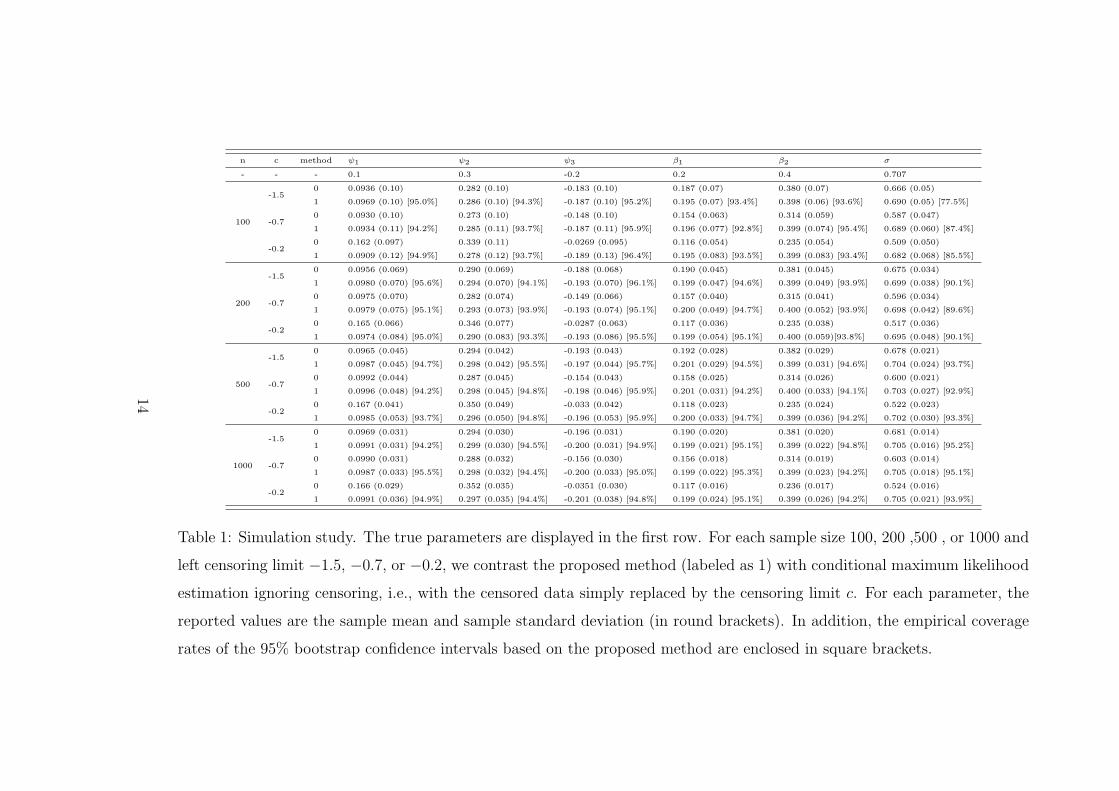
Table 1 reports the sample mean for each parameter estimate and their sample stan-

dard deviations enclosed in round brackets, for both methods. In addition, the empirical

coverage rates of the 95% confidence interval obtained by parametric bootstrap are listed

in square brackets, but only for the proposed method because conditional maximum likeli-

hood estimation ignoring censoring is quite biased for the case of moderately high censoring

rate.

It can be seen that the proposed method performed well in all cases, while ignoring

censoring led to increasing bias with the censoring rate. For both methods, the variance

of the estimator increased with the censoring rate and decreased with the sample size.

Parametric bootstrap seems to work well as the empirical coverage rates of the bootstrap

confidence intervals were quite close to the nominal 95%.

13

n c method ψ1 ψ2 ψ3 β1 β2 σ

- - - 0.1 0.3 -0.2 0.2 0.4 0.707

100

-1.50 0.0936 (0.10) 0.282 (0.10) -0.183 (0.10) 0.187 (0.07) 0.380 (0.07) 0.666 (0.05)

1 0.0969 (0.10) [95.0%] 0.286 (0.10) [94.3%] -0.187 (0.10) [95.2%] 0.195 (0.07) [93.4%] 0.398 (0.06) [93.6%] 0.690 (0.05) [77.5%]

-0.70 0.0930 (0.10) 0.273 (0.10) -0.148 (0.10) 0.154 (0.063) 0.314 (0.059) 0.587 (0.047)

1 0.0934 (0.11) [94.2%] 0.285 (0.11) [93.7%] -0.187 (0.11) [95.9%] 0.196 (0.077) [92.8%] 0.399 (0.074) [95.4%] 0.689 (0.060) [87.4%]

-0.20 0.162 (0.097) 0.339 (0.11) -0.0269 (0.095) 0.116 (0.054) 0.235 (0.054) 0.509 (0.050)

1 0.0909 (0.12) [94.9%] 0.278 (0.12) [93.7%] -0.189 (0.13) [96.4%] 0.195 (0.083) [93.5%] 0.399 (0.083) [93.4%] 0.682 (0.068) [85.5%]

200

-1.50 0.0956 (0.069) 0.290 (0.069) -0.188 (0.068) 0.190 (0.045) 0.381 (0.045) 0.675 (0.034)

1 0.0980 (0.070) [95.6%] 0.294 (0.070) [94.1%] -0.193 (0.070) [96.1%] 0.199 (0.047) [94.6%] 0.399 (0.049) [93.9%] 0.699 (0.038) [90.1%]

-0.70 0.0975 (0.070) 0.282 (0.074) -0.149 (0.066) 0.157 (0.040) 0.315 (0.041) 0.596 (0.034)

1 0.0979 (0.075) [95.1%] 0.293 (0.073) [93.9%] -0.193 (0.074) [95.1%] 0.200 (0.049) [94.7%] 0.400 (0.052) [93.9%] 0.698 (0.042) [89.6%]

-0.20 0.165 (0.066) 0.346 (0.077) -0.0287 (0.063) 0.117 (0.036) 0.235 (0.038) 0.517 (0.036)

1 0.0974 (0.084) [95.0%] 0.290 (0.083) [93.3%] -0.193 (0.086) [95.5%] 0.199 (0.054) [95.1%] 0.400 (0.059)[93.8%] 0.695 (0.048) [90.1%]

500

-1.50 0.0965 (0.045) 0.294 (0.042) -0.193 (0.043) 0.192 (0.028) 0.382 (0.029) 0.678 (0.021)

1 0.0987 (0.045) [94.7%] 0.298 (0.042) [95.5%] -0.197 (0.044) [95.7%] 0.201 (0.029) [94.5%] 0.399 (0.031) [94.6%] 0.704 (0.024) [93.7%]

-0.70 0.0992 (0.044) 0.287 (0.045) -0.154 (0.043) 0.158 (0.025) 0.314 (0.026) 0.600 (0.021)

1 0.0996 (0.048) [94.2%] 0.298 (0.045) [94.8%] -0.198 (0.046) [95.9%] 0.201 (0.031) [94.2%] 0.400 (0.033) [94.1%] 0.703 (0.027) [92.9%]

-0.20 0.167 (0.041) 0.350 (0.049) -0.033 (0.042) 0.118 (0.023) 0.235 (0.024) 0.522 (0.023)

1 0.0985 (0.053) [93.7%] 0.296 (0.050) [94.8%] -0.196 (0.053) [95.9%] 0.200 (0.033) [94.7%] 0.399 (0.036) [94.2%] 0.702 (0.030) [93.3%]

1000

-1.50 0.0969 (0.031) 0.294 (0.030) -0.196 (0.031) 0.190 (0.020) 0.381 (0.020) 0.681 (0.014)

1 0.0991 (0.031) [94.2%] 0.299 (0.030) [94.5%] -0.200 (0.031) [94.9%] 0.199 (0.021) [95.1%] 0.399 (0.022) [94.8%] 0.705 (0.016) [95.2%]

-0.70 0.0990 (0.031) 0.288 (0.032) -0.156 (0.030) 0.156 (0.018) 0.314 (0.019) 0.603 (0.014)

1 0.0987 (0.033) [95.5%] 0.298 (0.032) [94.4%] -0.200 (0.033) [95.0%] 0.199 (0.022) [95.3%] 0.399 (0.023) [94.2%] 0.705 (0.018) [95.1%]

-0.20 0.166 (0.029) 0.352 (0.035) -0.0351 (0.030) 0.117 (0.016) 0.236 (0.017) 0.524 (0.016)

1 0.0991 (0.036) [94.9%] 0.297 (0.035) [94.4%] -0.201 (0.038) [94.8%] 0.199 (0.024) [95.1%] 0.399 (0.026) [94.2%] 0.705 (0.021) [93.9%]

Table 1: Simulation study. The true parameters are displayed in the first row. For each sample size 100, 200 ,500 , or 1000 and

left censoring limit −1.5, −0.7, or −0.2, we contrast the proposed method (labeled as 1) with conditional maximum likelihood

estimation ignoring censoring, i.e., with the censored data simply replaced by the censoring limit c. For each parameter, the

reported values are the sample mean and sample standard deviation (in round brackets). In addition, the empirical coverage

rates of the 95% bootstrap confidence intervals based on the proposed method are enclosed in square brackets.

14

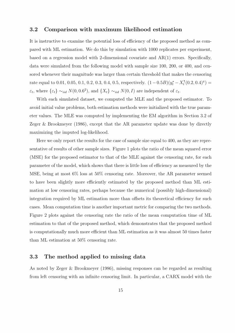
3.2 Comparison with maximum likelihood estimation

It is instructive to examine the potential loss of efficiency of the proposed method as com-

pared with ML estimation. We do this by simulation with 1000 replicates per experiment,

based on a regression model with 2-dimensional covariate and AR(1) errors. Specifically,

data were simulated from the following model with sample size 100, 200, or 400, and cen-

sored whenever their magnitude was larger than certain threshold that makes the censoring

rate equal to 0.01, 0.05, 0.1, 0.2, 0.3, 0.4, 0.5, respectively. (1−0.5B)(y∗t −Xᵀt (0.2, 0.4)

ᵀ) =

εt, where {εt} ∼iid N(0, 0.62), and {Xt} ∼iid N(0, I) are independent of εt.

With each simulated dataset, we computed the MLE and the proposed estimator. To

avoid initial value problems, both estimation methods were initialized with the true param-

eter values. The MLE was computed by implementing the EM algorithm in Section 3.2 of

Zeger & Brookmeyer (1986), except that the AR parameter update was done by directly

maximizing the imputed log-likelihood.

Here we only report the results for the case of sample size equal to 400, as they are repre-

sentative of results of other sample sizes. Figure 1 plots the ratio of the mean squared error

(MSE) for the proposed estimator to that of the MLE against the censoring rate, for each

parameter of the model, which shows that there is little loss of efficiency as measured by the

MSE, being at most 6% loss at 50% censoring rate. Moreover, the AR parameter seemed

to have been slightly more efficiently estimated by the proposed method than ML esti-

mation at low censoring rates, perhaps because the numerical (possibly high-dimensional)

integration required by ML estimation more than offsets its theoretical efficiency for such

cases. Mean computation time is another important metric for comparing the two methods.

Figure 2 plots against the censoring rate the ratio of the mean computation time of ML

estimation to that of the proposed method, which demonstrates that the proposed method

is computationally much more efficient than ML estimation as it was almost 50 times faster

than ML estimation at 50% censoring rate.

3.3 The method applied to missing data

As noted by Zeger & Brookmeyer (1986), missing responses can be regarded as resulting

from left censoring with an infinite censoring limit. In particular, a CARX model with the

15

0.0 0.1 0.2 0.3 0.4 0.5

1.00

1.01

1.02

1.03

1.04

1.05

1.06

Censoring rate

MS

E r

atio

(W

C/Z

B)

β1

β2ψ1

σ

Figure 1: MSE ratio of parameter estimates of the proposed method to MLE.

0.0 0.1 0.2 0.3 0.4 0.5

1020

3040

Censoring rate

Rat

io o

f mea

n co

mpu

tatio

n tim

e

Figure 2: Plot of the ratio of the mean computation time of maximum likelihood estimation

to that of the proposed method.

16

response missing at random provides another setting for comparing the proposed method

with Gaussian likelihood estimation which can be readily carried out via Kalman filtering as

implemented by the arima function in the stats package of R Core Team (2015); see Ripley

(2002). For this purpose, we simulated data from the model: (1 + 0.28B − 0.25B2)(y∗t −

Xᵀt (0.2, 0.4)

ᵀ) = εt, which is the same as the model in Section 3.2 except that the regression

errors now follow an AR(2) model. Data were simulated from the preceding model with

sample size equal to 100, 200, or 400, and data were subsequently discarded randomly to

make various missing rates, namely, 0.01, 0.05, 0.1, 0.2, 0.3, 0.4, 0.5, respectively. With

each simulated series, the CARX model was estimated once by ML estimation via the

arima function and once by the proposed method, again with the true parameter values as

the initial values. The results were similar across different sample sizes, so we only report

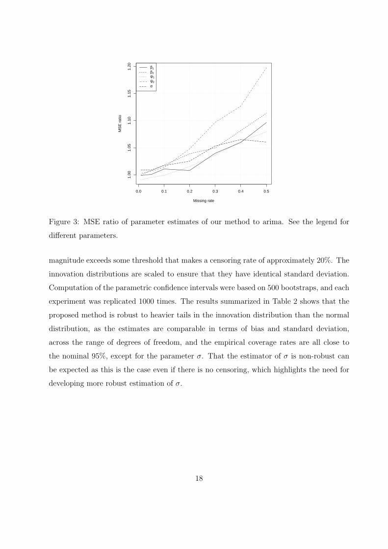
the results for sample size equal to 400. Figure 3 plots against the missing rate the ratio of

the MSE of the proposed method to that of the ML estimation, for each parameter, which

shows that the MSE of the proposed method is less than 5% higher than ML estimation

for missing rate up to 20%, and is generally not more than 10% higher even at 50% missing

rate, except for the parameter σ.

Taken together, the simulation studies in this and previous sub-sections indicate that

the proposed method generally incurs relatively little loss of efficiency compared with ML

estimation.

3.4 The robustness of the proposed method

As the proposed method may also be regarded as a generalization of Gaussian likelihood

estimation or conditional least squares, it is of interest to assess its robustness against

departure from the normal innovation assumption. We did this with a simulation study

where the innovations were t-distributed, while the model estimation was done based on

normal innovations.

Data were simulated from a CARX model with independent 2-dimensional standard

normal covariates and AR(3) errors with t-distributed innovations of degrees of freedom

equal to 5, 10, 20, or ∞ (i.e. normal distribution), and sample size equal to 100, 200 or 400.

See Table 2 for the true parameter values. The responses were censored whenever their

17

0.0 0.1 0.2 0.3 0.4 0.5

1.00

1.05

1.10

1.15

1.20

Missing rate

MS

E r

atio

β1

β2ψ1

ψ2

σ

Figure 3: MSE ratio of parameter estimates of our method to arima. See the legend for

different parameters.

magnitude exceeds some threshold that makes a censoring rate of approximately 20%. The

innovation distributions are scaled to ensure that they have identical standard deviation.

Computation of the parametric confidence intervals were based on 500 bootstraps, and each

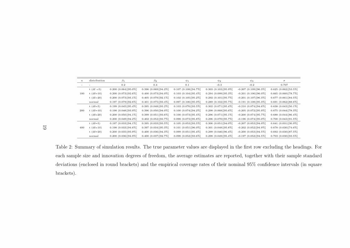
experiment was replicated 1000 times. The results summarized in Table 2 shows that the

proposed method is robust to heavier tails in the innovation distribution than the normal

distribution, as the estimates are comparable in terms of bias and standard deviation,

across the range of degrees of freedom, and the empirical coverage rates are all close to

the nominal 95%, except for the parameter σ. That the estimator of σ is non-robust can

be expected as this is the case even if there is no censoring, which highlights the need for

developing more robust estimation of σ.

18

n distribution β1 β2 ψ1 ψ2 ψ3 σ

- - 0.2 0.4 0.1 -0.3 -0.2 0.707

100

t (df =5) 0.200 (0.064)[95.0%] 0.396 (0.069)[94.2%] 0.107 (0.108)[94.7%] 0.303 (0.103)[95.9%] -0.207 (0.109)[96.3%] 0.625 (0.062)[53.5%]

t (df=10) 0.200 (0.073)[92.6%] 0.400 (0.073)[94.0%] 0.103 (0.104)[95.4%] 0.294 (0.099)[95.3%] -0.201 (0.106)[96.0%] 0.665 (0.060)[78.7%]

t (df=20) 0.200 (0.073)[93.1%] 0.405 (0.079)[92.1%] 0.102 (0.105)[95.2%] 0.292 (0.101)[95.7%] -0.201 (0.107)[96.3%] 0.677 (0.061)[84.5%]

normal 0.197 (0.079)[92.6%] 0.401 (0.075)[93.4%] 0.097 (0.106)[95.0%] 0.289 (0.102)[95.7%] -0.191 (0.108)[95.3%] 0.691 (0.062)[88.6%]

200

t (df=5) 0.199 (0.045)[95.4%] 0.395 (0.048)[93.2%] 0.103 (0.076)[93.5%] 0.302 (0.071)[95.4%] -0.210 (0.074)[94.6%] 0.638 (0.043)[50.1%]

t (df=10) 0.198 (0.048)[93.9%] 0.396 (0.050)[94.0%] 0.100 (0.074)[94.2%] 0.298 (0.068)[95.6%] -0.205 (0.072)[95.9%] 0.675 (0.044)[78.3%]

t (df=20) 0.200 (0.050)[94.1%] 0.399 (0.051)[93.6%] 0.100 (0.073)[95.4%] 0.296 (0.071)[95.1%] -0.200 (0.074)[95.7%] 0.688 (0.044)[86.4%]

normal 0.200 (0.049)[94.2%] 0.402 (0.052)[93.7%] 0.098 (0.073)[95.8%] 0.296 (0.070)[95.7%] -0.196 (0.074)[95.0%] 0.700 (0.043)[91.5%]

400

t (df=5) 0.197 (0.033)[94.1%] 0.395 (0.033)[93.5%] 0.105 (0.053)[93.5%] 0.306 (0.051)[94.0%] -0.207 (0.053)[94.0%] 0.641 (0.031)[30.9%]

t (df=10) 0.198 (0.033)[94.6%] 0.397 (0.034)[95.3%] 0.101 (0.051)[96.0%] 0.301 (0.048)[95.8%] -0.202 (0.052)[94.9%] 0.678 (0.030)[74.6%]

t (df=20) 0.200 (0.035)[93.9%] 0.400 (0.036)[94.3%] 0.099 (0.051)[95.4%] 0.299 (0.046)[96.4%] -0.200 (0.053)[94.5%] 0.692 (0.030)[87.5%]

normal 0.200 (0.036)[94.9%] 0.400 (0.037)[92.7%] 0.098 (0.052)[93.6%] 0.298 (0.049)[95.4%] -0.197 (0.052)[94.5%] 0.703 (0.030)[93.5%]

Table 2: Summary of simulation results. The true parameter values are displayed in the first row excluding the headings. For

each sample size and innovation degrees of freedom, the average estimates are reported, together with their sample standard

deviations (enclosed in round brackets) and the empirical coverage rates of their nominal 95% confidence intervals (in square

brackets).

19

3.5 The Ljung-Box test statistic based on simulated residuals

Next, we report some simulation results on the empirical performance of the Ljung-Box test

statistic, based on the simulated residuals, that is used as a tool for model diagnostics. The

null model is an AR(2) model with a two-dimensional covariate comprising two independent

standard normal variables, with βᵀ= (0.2, 0.4), ψ

ᵀ= (0.28, 0.25), and σ = 0.6. We

computed the Ljung-Box statistic using the first 10 or 20 lags of the sample autocorrelation

function (ACF) of the simulated residuals. For assessing the power of the test, the AR part

of the model is embedded in an AR(3) model with the AR operator given by (1− δB)(1−

Ψ(B)), where δ = 0.0, 0.1, 0.2, · · · , 0.8. The data are left-censored so as to achieve a long-

run censoring rate of 15%, or 30%, plus the case of no censoring as a benchmark, with

sample size 100, or 200. The empirical rejection rates based on 1000 replications are shown

in Figure 4. The sizes of the test under all settings are quite close to the nominal 5% level.

The power generally increases with greater deviation of δ from zero, lesser censoring, larger

sample size and fewer lags used in computing the Ljung-Box statistic. That using more

lags in the test resulted in lower power is expected owing to the geometric decay of the

ACF so that its higher lags quickly become non-informative.

3.6 An application to the total phosphorus concentration in river

water

Phosphorus is one of the two nutrients of main concern in Iowa river water, as excessive

phosphorus in river water can result in eutrophication. Phosphorus concentration in river

water has been closely monitored under the ambient water quality program conducted by

the Iowa Department of Natural Resources (Libra, Wolter & Langel 2004). Here, we analyze

a series of 120 monthly phosphorus concentration (P) in mg/l, in river water collected at

an ambient site located at Whitebreast Creek near Knoxville, Iowa, USA, from October

1998 to March 2010. There is a gap of missing P data from September 2008 to March 2009,

when data collection was suspended owing to lack of funding. The data were censored

when P fell below certain detection limits ct (red line in Figure 5) that varied over time,

resulting in about 10% censoring. It is known that P is generally correlated with the water

discharge (Q) (Schilling, Chan, Liu & Zhang 2010). The main interest is to explore the

20

Figure 4: Empirical rejection rates of the Ljung-Box test with (simulated) residuals. The

left and right plots correspond to sample size 100 and 200, respectively. Empirical rejection

rates are connected with a solid line for the test using the first 10 lags of residual ACF and

no censoring, while those from experiments with left-censored data at long-run censoring

rate of 15% (30%) are connected with a dashed (dotted) line. Their counterparts for the

test based on first 20 lags of residual ACF are similarly plotted except that the rates are

superimposed as solid circles. A horizontal solid line is illustrated in both plots representing

the nominal 5% size.

21

relationship between P and Q with censored P data. The Q data were obtained from the

website of the U.S. Geological Survey. See Figure 5 for the time plots of P, Q, and the

historical censoring limits.

Oct1999

Oct2000

Oct2001

Oct2002

Oct2003

Oct2004

Oct2005

Oct2006

Oct2007

Oct2008

Oct2009

0.0

0.5

1.0

1.5

2.0

2.5

3.0

3.5

Time

P

020

0040

0060

0080

00

Q

PCensor limitQ

Figure 5: Time series plots of P (black solid line, scale shown on the left vertical axis), Q

(blue dotted line, scale shown on the right vertical axis) and the censoring limits ct (red

dashed line, in the same scale as that of P).

Preliminary analysis (unreported) shows that taking the logarithmic transformation for

both P and Q renders their relationship more linear. Model diagnostics with a preliminary

linear regression model log(Pt) = β0 + β1 log(Qt) + ηt indicates (i) the presence of serial

residual autocorrelation, hence we model ηt as an autoregressive process, and (ii) that the

P-Q relationship is seasonal. We model the seasonal relationship by introducing the dummy

seasonal dummy variables Sj, j = 1, 2, 3, 4 for quarters 1 to 4 and their interactions with

discharge log(Qt), where the first quarter comprises January to March, the second quarter

22

from April to June, etc. In summary, the model is

log(Pt) =4∑

j=1

{β0,jSj,t + β1,jSj,t × log(Qt)}+ ηt,

where the regression errors {ηt} follow an autoregressive model as defined in Eq (2) with εt

independent and identically distributed as N(0, σ2). The coefficients β0,1 and β1,1 are the

intercept and slope for quarter 1, β0,2 and β1,2 those for quarter 2, etc.

Since the AR order is unknown and the seasonal P-Q relationship is uncertain, we fitted

a number of models with or without seasonal P-Q relationship and the AR order from 0

to 3, altogether 8 models. Model selection was then carried out by using an information

criterion similar to the AIC with the log-likelihood replaced by the conditional expectation

defined in Eq (8). A seasonal regression model with AR(2) regression errors was selected.

The final model fit is summarized in Table 3; the parametric bootstrap 95% confidence

intervals are based on 1000 replicates. The P-Q relationships in quarters 2 and 4 are

quite similar. Indeed, constraining the regression coefficients to be identical for these two

quarters slightly reduces the AIC from 17.027 to 17.013. The rate of change in log(P ) per

unit change in log(Q) is highest in quarter 1 and lowest in quarter 3; see Figure 6 which

shows the simulated partial residual plot of log(Q) (c.f. Subsection 2.6), with the fitted

quarterly linear relationships superimposed in the diagram. These found relationships are

consistent with the fact that discharge is generally lowest in quarter 1 and highest in

quarter 3. The AR estimates are moderate in values, suggesting rather short memory in

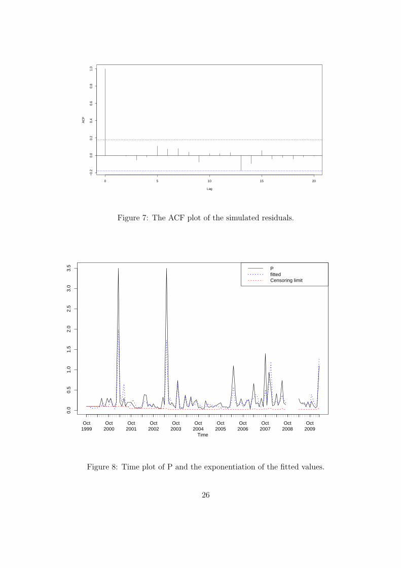
the data. Figure 7 plots the ACF of the simulated residuals, which suggests no residual

autocorrelation. The Ljung-Box test statistic using the first 10 lags of the residual ACF is

5.28 with p-value 0.27, suggesting no serial autocorrelation in the residuals and that the

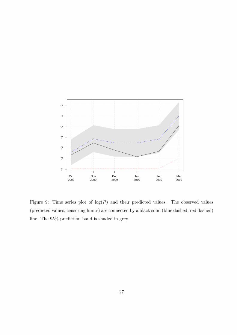
model provides a good fit to the data. Finally, Figure 8 plots the time plot of P and the

exponentiation of the fitted values, showing that the fitted values generally track the data

well, but less so for the larger P peaks.

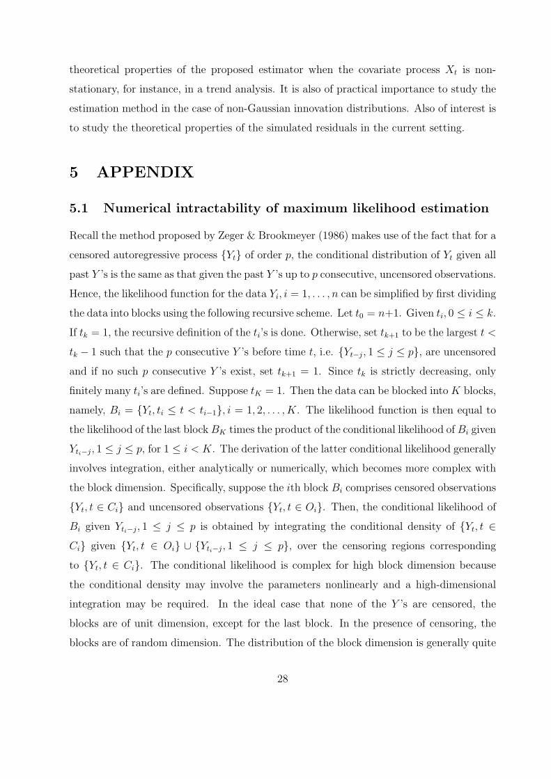
As an illustration of prediction with a censored time series, we re-fitted the selected

model with the data excluding the last 6 observations that are withheld for assessing

the real prediction performance. The point predictors and their 95% prediction intervals,

computed using procedure elaborated in Section 2.5 and assuming normal innovations,

are shown in Figure 9, with the actual data superimposed on the diagram. Overall, the

23

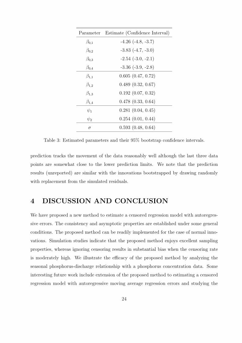
Parameter Estimate (Confidence Interval)

β0,1 -4.26 (-4.8, -3.7)

β0,2 -3.83 (-4.7, -3.0)

β0,3 -2.54 (-3.0, -2.1)

β0,4 -3.36 (-3.9, -2.8)

β1,1 0.605 (0.47, 0.72)

β1,2 0.489 (0.32, 0.67)

β1,3 0.192 (0.07, 0.32)

β1,4 0.478 (0.33, 0.64)

ψ1 0.281 (0.04, 0.45)

ψ2 0.254 (0.01, 0.44)

σ 0.593 (0.48, 0.64)

Table 3: Estimated parameters and their 95% bootstrap confidence intervals.

prediction tracks the movement of the data reasonably well although the last three data

points are somewhat close to the lower prediction limits. We note that the prediction

results (unreported) are similar with the innovations bootstrapped by drawing randomly

with replacement from the simulated residuals.

4 DISCUSSION AND CONCLUSION

We have proposed a new method to estimate a censored regression model with autoregres-

sive errors. The consistency and asymptotic properties are established under some general

conditions. The proposed method can be readily implemented for the case of normal inno-

vations. Simulation studies indicate that the proposed method enjoys excellent sampling

properties, whereas ignoring censoring results in substantial bias when the censoring rate

is moderately high. We illustrate the efficacy of the proposed method by analyzing the

seasonal phosphorus-discharge relationship with a phosphorus concentration data. Some

interesting future work include extension of the proposed method to estimating a censored

regression model with autoregressive moving average regression errors and studying the

24

2 4 6 8

−5

−4

−3

−2

−1

01

2

log(Q)

Par

tial R

esid

ual

Figure 6: Partial residual plot for log(Q), with a partial residual drawn as an open circle

(triangle, plus, cross), if it belongs to quarter 1 (2,3,4). The four lines display the quar-

terly linear relationship, with solid, dashed, dotted, dot-dashed lines for quarters 1,2,3,4,

respectively.

25

0 5 10 15 20

−0.

20.

00.

20.

40.

60.

81.

0

Lag

AC

F

Figure 7: The ACF plot of the simulated residuals.

Oct1999

Oct2000

Oct2001

Oct2002

Oct2003

Oct2004

Oct2005

Oct2006

Oct2007

Oct2008

Oct2009

0.0

0.5

1.0

1.5

2.0

2.5

3.0

3.5

Time

PfittedCensoring limit

Figure 8: Time plot of P and the exponentiation of the fitted values.

26

Oct2009

Nov2009

Dec2009

Jan2010

Feb2010

Mar2010

−4

−3

−2

−1

01

2

Figure 9: Time series plot of log(P ) and their predicted values. The observed values

(predicted values, censoring limits) are connected by a black solid (blue dashed, red dashed)

line. The 95% prediction band is shaded in grey.

27

theoretical properties of the proposed estimator when the covariate process Xt is non-

stationary, for instance, in a trend analysis. It is also of practical importance to study the

estimation method in the case of non-Gaussian innovation distributions. Also of interest is

to study the theoretical properties of the simulated residuals in the current setting.

5 APPENDIX

5.1 Numerical intractability of maximum likelihood estimation

Recall the method proposed by Zeger & Brookmeyer (1986) makes use of the fact that for a

censored autoregressive process {Yt} of order p, the conditional distribution of Yt given all

past Y ’s is the same as that given the past Y ’s up to p consecutive, uncensored observations.

Hence, the likelihood function for the data Yi, i = 1, . . . , n can be simplified by first dividing

the data into blocks using the following recursive scheme. Let t0 = n+1. Given ti, 0 ≤ i ≤ k.

If tk = 1, the recursive definition of the ti’s is done. Otherwise, set tk+1 to be the largest t <

tk − 1 such that the p consecutive Y ’s before time t, i.e. {Yt−j, 1 ≤ j ≤ p}, are uncensored

and if no such p consecutive Y ’s exist, set tk+1 = 1. Since tk is strictly decreasing, only

finitely many ti’s are defined. Suppose tK = 1. Then the data can be blocked intoK blocks,

namely, Bi = {Yt, ti ≤ t < ti−1}, i = 1, 2, . . . , K. The likelihood function is then equal to

the likelihood of the last block BK times the product of the conditional likelihood of Bi given

Yti−j, 1 ≤ j ≤ p, for 1 ≤ i < K. The derivation of the latter conditional likelihood generally

involves integration, either analytically or numerically, which becomes more complex with

the block dimension. Specifically, suppose the ith block Bi comprises censored observations

{Yt, t ∈ Ci} and uncensored observations {Yt, t ∈ Oi}. Then, the conditional likelihood of

Bi given Yti−j, 1 ≤ j ≤ p is obtained by integrating the conditional density of {Yt, t ∈

Ci} given {Yt, t ∈ Oi} ∪ {Yti−j, 1 ≤ j ≤ p}, over the censoring regions corresponding

to {Yt, t ∈ Ci}. The conditional likelihood is complex for high block dimension because

the conditional density may involve the parameters nonlinearly and a high-dimensional

integration may be required. In the ideal case that none of the Y ’s are censored, the

blocks are of unit dimension, except for the last block. In the presence of censoring, the

blocks are of random dimension. The distribution of the block dimension is generally quite

28

complex. As a benchmark, assuming independent censoring and a constant censoring rate,

say π (which holds if the uncensored process is independent and identically distributed, and

censoring occurs when the underlying process falls within some fixed interval), the mean

block dimension, excluding the last block BK , can be shown to be {1− (1− π)p}/{π(1−

π)p}−p+1, with variance equal to {1− (2p+1)π(1−π)p− (1−π)2p+1}/{π2(1−π)2p}; see

Philippou, Georghiou & Philippou (1983). For instance, for p = 5 and a 25% censoring rate,

the mean block dimension is ≈ 8.9 with standard deviation about 9.3. So, relatively high

dimensional integration may be required even for p = 5 to carry out maximum likelihood

estimation, rendering the method increasingly computationally intensive with the censoring

rate.

5.2 Proof of Theorem 2.1

Proof. First, note that the function Zt(θ) is continuously differentiable with respect to θ.

By A1, a consistent initial estimate for the parameter is assumed, so the parameter space

is restricted to some compact neighbourhood Θ of θ0, which is assumed to satisfy some

conditions specified below.

The functional central limit theorem of Arcones & Yu (1994) will be used to prove

{√n(Z(n)(θ)− Eθ0 [Zt(θ)]

): θ ∈ Θ

} L−→ {G(θ) : θ ∈ Θ},

where {G(θ)} is a Gaussian process which has a version with uniformly bounded and

uniformly continuous sample paths with respect to the L2 norm. See also Chan & Tsay

(1998). In order to apply the alluded functional central limit theorem to {Zt}, we need to

verify that

1 the class of functions {Zt(θ), θ ∈ Θ} is a Vapnick-Cervonenkis subgraph class of mea-

surable functions,

2 there exists an envelope function F ∈ Lp for some p > 2 such that |Zt(θ)| ≤ F for all

θ ∈ Θ, and

3 The process {(Y ∗t , Xt, ct,l, ct,u)} is stationary, β-mixing with a geometrically decaying

β-mixing rate.

29

The first two conditions are essentially stated by A6. The third condition is ensured by

A2–A5.

We verify the consistency result by using Theorem 5.9 of Van der Vaart (2000), with

the key steps established below. Firstly, we show that θ0 is a zero of Z(θ):

Eθ0 [Zt(θ0)]

=Eθ0

[Eθ0

[∂ℓ(Y ∗

t |F∗t , θ)

∂θ|θ=θ0|Gt

]]=Eθ0

[∂ℓ(Y ∗

t |F∗t , θ)

∂θ|θ=θ0

]=Eθ0

[Eθ0

[∂ℓ(Y ∗

t |F∗t , θ)

∂θ|θ=θ0|F∗

t

]]=Eθ0 [0]

=0.

It follows from A7 that for any small enough ε > 0, Eθ0 [∇Zt(θ)] is non-singular for all θ

such that ∥θ − θ0∥ < ε. As Z(θ) = Z(θ0) +∇Zt(θ0)ᵀ(θ − θ0) + o(∥θ − θ0∥) around θ0, the

non-singularity of ∇Z around θ0 implies that for all sufficiently small ϵ > 0, Z(θ) = 0 for

all ∥θ− θ0∥ < ε and θ = θ0, and further it holds that infθ∈Θ,∥θ−θ0∥>ε ∥Eθ0 [Zt(θ)] ∥ > 0. The

uniform convergence

supθ∈Θ

∥Z(n)(θ)− Z(θ)∥ P−→ 0

follows from the functional limit theorem for Zt(θ). The consistency property then follows

from Theorem 5.9 of Van der Vaart (2000).

The asymptotic normality result can be verified by using similar techniques in the proof

of Theorem 5.21 of Van der Vaart (2000) and Arcones & Yu (1994).

5.3 Verification of Assumption A6 for the case of normal inno-

vations

Proposition 5.1. Assumptions A6 and A7 hold if the innovations are normally distributed,

exp(ϵ∥Xt∥2) ∈ L1 for some small ϵ > 0, and the parameter space is a sufficiently small

neighborhood of θ0.

30

Proof. First note that the score function has the following form,

S(Y ∗t |F∗

t , θ) =1

σ2

εt(Xt −

∑pj=1 ψjXt−j)

εtηt−1:t−p

12

(1− ε2t

σ2

)

where ηt = Y ∗t −Xᵀ

t β and εt = (1−Ψ(B))ηt.

Expanding each term in the score function, it is seen that each element in the vector

Zt(θ) can be written as some linear combination of the following terms

Eθ

[(Y ∗

t−i)j|Gt

]∥Xt−l∥m, (13)

where (i) i, l = 0, . . . , p; (ii) j,m = 0, 1, 2; and (iii) j +m ≤ 2.

To show the V-C property for Zt(θ), it suffices to show that Eθ

[(Y ∗

t−i)j|Gt

]is a V-C

class, then so is Zt(θ). For truncated normal distributions, Tallis (1961) gives the closed-

form expressions for the moments of first and second orders, from which the V-C property

can be deduced. (Note that the V-C property is preserved by forming finite products and

sums of elements of a V-C class.)

It remains to find an envelope function for the score functions Zt(θ). It suffices to first

find some envelope functions for the expression defined by Eq (13).

As the main difficulty lies in bounding Eθ

[(Y ∗

t−i)j|Gt

], we first present a general result

about conditional expectation and change of measure. Suppose we have a conditional

expectation Eθ [W |G] where W is some random variable and G is a relevant σ-algebra, and

θ is the parameter indexing the underlying probability measure to be denoted as Pθ, where

θ lies in Nθ0 , a neighborhood of a known parameter θ0. We want to find simple conditions

sufficient for the existence of an envelope function for Eθ [W |G] for θ ∈ Nθ0 that has finite

absolute q-th moment under Pθ0 .

Suppose Pθ, θ ∈ Nθ0 are pairwise mutually absolutely continuous so thatdPθ1dPθ2

is well-

defined for all θ1, θ2 ∈ Nθ0 . The following lemma is instrumental, whose proof is deferred

to later.

Lemma 5.2.

Eθ(W |G) = Eθ0

(W

dPθ

dPθ0

|G)Eθ

(dPθ0

dPθ

|G). (14)

31

Setting W ≡ 1 in (14) yields the identity

Eθ

(dPθ0

dPθ

|G)

= E−1θ0

(dPθ

dPθ0

|G).

Hence,

Eθ(W |G) = Eθ0

(W

dPθ

dPθ0

|G)E−1

θ0

(dPθ

dPθ0

|G).

Jensen’s inequality then implies that

|Eθ(W |G)| ≤ Eθ(|W ||G) = Eθ0

(|W | dPθ

dPθ0

∣∣∣∣G)E−1θ0

(dPθ

dPθ0

∣∣∣∣G) .As the function f(x) = 1/x, x > 0 is convex, Jensen’s inequality entails that

|Eθ(W |G)| ≤ Eθ0

(|W | dPθ

dPθ0

|G)Eθ0

(dPθ0

dPθ

|G). (15)

We shall assume that the neighborhood Nθ0 is chosen such that there exists a random

variable H of finite absolute r-th moment under Pθ0 and such thatdPθ1dPθ2

≤ H for all θ1, θ2 ∈

Nθ0 . It then follows from (15) that

supθ∈Nθ0

|Eθ(W |G)| ≤ Eθ0 (|W |H|G)Eθ0 (H|G) . (16)

The right side of (16) is then an envelope function of {Eθ(W |G), θ ∈ Nθ0}.

We now consider the case of normally distributed innovations in our model, in which

case the conditional distribution of Y ∗t:t−p given theX’s is multivariate normalN(xᵀt:t−pβ,Σ),

where Σ is determined by ψ and σ. Let y = yt:t−p and µi = xᵀt:t−pβi, i = 0, 1, 2. Direct

calculation yields

dPθ1

dPθ2

(y) = exp

(yᵀΣ−1

1 (µ1 − µ2)−1

2(µ1 + µ2)Σ

−11 (µ1 − µ2)

)×(|Σ2||Σ1|

)n/2

exp

(−1

2(y − µ2)

ᵀΣ−11 (Σ1 − Σ2) Σ

−12 (y − µ2)

)≤c exp

(ϵ(∥y − µ0∥2 + ∥xt:t−p∥2)

):=H,

where c is some constant independent of θ1, θ2, and ϵ can be arbitrarily small as long as

the neighborhood Nθ0 is sufficiently small. Then or any r > 0,

Eθ0 [Hr] =Eθ0 [Eθ0 [H

r| xt:t−p]]

=cEθ0

[exp(rϵ∥xt:t−p∥2)

]Eθ0

[exp(rϵ∥y − µ0∥2)

∣∣xt:t−p

]=cEθ0

[exp(rϵ∥xt:t−p∥2)

]Eθ0

[exp(rϵ∥y − µ0∥2)

],

32

which is finite when ϵ is small enough by the assumption that exp(rϵ∥Xt∥2) ∈ L1.

It follows from E [exp(ϵ∥Xt∥2)] <∞ for some ϵ > 0 that Xt has finite moments of any fi-

nite order. An envelope function for the expression in Eq (13) is Eθ0

(|Y ∗

t−i|jH|Gt

)Eθ0 (H|Gt) ∥Xt−l∥m.

Because Y ∗t−j given the X’s is normal, it admits finite moments of any order. It follows

from the generalized Holder inequality and by making the neighborhood Nθ0 sufficiently

small that |Yt−i|jHEθ0 [H|Gt]∥Xt−l∥m is Lq and so is the envelope function.

Proof of Lemma 5.2. Note that the conditional expectation Eθ(W |G) is characterized by

(i) Eθ(W |G) is G-measurable function and (ii) for all A ∈ G, the following equality holds:∫A

WdPθ =

∫A

Eθ(W |G)dPθ.

Consider the following display, where A is an arbitrary element in G:∫A

WdPθ =

∫A

WdPθ

dPθ0

dPθ0

=

∫A

Eθ0

(W

dPθ

dPθ0

|G)dPθ0

=

∫A

Eθ0

(W

dPθ

dPθ0

|G)dPθ0

dPθ

dPθ

=

∫A

Eθ0

(W

dPθ

dPθ0

|G)Eθ

(dPθ0

dPθ

|G)dPθ.

The claim follows from the preceding equality and that the right side of (14) is G-measurable.

33

References

Amemiya, T. (1973), “Regression analysis when the dependent variable is truncated nor-

mal,” Econometrica: Journal of the Econometric Society, pp. 997–1016.

Arcones, M. A., & Yu, B. (1994), “Central limit theorems for empirical and U-processes of

stationary mixing sequences,” Journal of Theoretical Probability, 7(1), 47–71.

Buckley, J., & James, I. (1979), “Linear regression with censored data,” Biometrika,

66(3), 429–436.

Chan, K.-S., & Tsay, R. S. (1998), “Limiting properties of the least squares estimator of a

continuous threshold autoregressive model,” Biometrika, 85(2), 413–426.

Cox, D. R., & Snell, E. J. (1968), “A general definition of residuals,” Journal of the Royal

Statistical Society. Series B (Methodological), pp. 248–275.

Cryer, J. D., & Chan, K. S. (2008), Time series analysis: with applications in R, New

York: Springer.

Genz, A., & Bretz, F. (2009), Computation of Multivariate Normal and t Probabilities,

Lecture Notes in Statistics, Heidelberg: Springer-Verlag.

Genz, A., Bretz, F., Miwa, T., Mi, X., Leisch, F., Scheipl, F., & Hothorn, T. (2014),

mvtnorm: Multivariate Normal and t Distributions. R package version 1.0-0.

Gourieroux, C., Monfort, A., Renault, E., & Trognon, A. (1987), “Simulated residuals,”

Journal of Econometrics, 34(1), 201–252.

Hillis, S. L. (1995), “Residual plots for the censored data linear regression model,” Statistics

in medicine, 14(18), 2023–2036.

Jawitz, J. W. (2004), “Moments of truncated continuous univariate distributions,” Ad-

vances in water resources, 27(3), 269–281.

Libra, R. D., Wolter, C. F., & Langel, R. J. (2004), Nitrogen and phosphorus budgets for

Iowa and Iowa watersheds Iowa Department of Natural Resources, Geological Survey.

34

Park, J. W., Genton, M. G., & Ghosh, S. K. (2007), “Censored time series analysis with

autoregressive moving average models,” Canadian Journal of Statistics, 35(1), 151–

168.

Pham, T. D., & Tran, L. T. (1985), “Some mixing properties of time series models,”

Stochastic processes and their applications, 19(2), 297–303.

Philippou, A. N., Georghiou, C., & Philippou, G. N. (1983), “A generalized geometric

distribution and some of its properties,” Statistics & Probability Letters, 1(4), 171–

175.

R Core Team (2015), R: A Language and Environment for Statistical Computing, R Foun-

dation for Statistical Computing.

Ripley, B. D. (2002), “Time series in R 1.5. 0,” R News, 2(2), 2–7.

Robinson, P. M. (1980), Estimation and forecasting for time series containing censored or

missing observations,, in Time Series: Proceedings of the International Conference,

Held at Nottingham University, March, 1979, ed. O. D. Anderson, North Holland,

pp. 167–182.

Robinson, P. M. (1982a), “On the asymptotic properties of estimators of models contain-

ing limited dependent variables,” Econometrica: Journal of the Econometric Society,

pp. 27–41.

Robinson, P. M. (1982b), “Analysis of time series from mixed distributions,” The Annals

of Statistics, pp. 915–925.

Schilling, K. E., Chan, K. S., Liu, H., & Zhang, Y. K. (2010), “Quantifying the effect of

land use land cover change on increasing discharge in the Upper Mississippi River,”

Journal of Hydrology, 387(3), 343–345.

Tallis, G. M. (1961), “The Moment Generating Function of the Truncated Multi-normal

Distribution,” Journal of the Royal Statistical Society. Series B (Methodological),

23(1), 223–229.

35

Tobin, J. (1958), “Estimation of relationships for limited dependent variables,” Economet-

rica: journal of the Econometric Society, pp. 24–36.

Van der Vaart, A. W. (2000), Asymptotic statistics, Vol. 3, Cambridge: Cambridge univer-

sity press.

Zeger, S. L., & Brookmeyer, R. (1986), “Regression Analsis with Censored Autocorrelated

Data,” Journal of the American Statistical Association, 81(395), 722–729.

36