QUASI-LINEAR COMPRESSED SENSING 1. Introduction

QUASI-LINEAR COMPRESSED SENSING

MARTIN EHLER∗, MASSIMO FORNASIER† , AND JULIANE SIGL‡

Abstract. Inspired by significant real-life applications, in particular, sparse phase retrieval and sparse pulsation fre-quency detection in Asteroseismology, we investigate a general framework for compressed sensing, where the measurements arequasi-linear. We formulate natural generalizations of the well-known Restricted Isometry Property (RIP) towards nonlinearmeasurements, which allow us to prove both unique identifiability of sparse signals as well as the convergence of recoveryalgorithms to compute them efficiently. We show that for certain randomized quasi-linear measurements, including Lipschitzperturbations of classical RIP matrices and phase retrieval from random projections, the proposed restricted isometry propertieshold with high probability. We analyze a generalized Orthogonal Least Squares (OLS) under the assumption that magnitudesof signal entries to be recovered decay fast. Greed is good again, as we show that this algorithm performs efficiently in phaseretrieval and Asteroseismology. For situations where the decay assumption on the signal does not necessarily hold, we proposetwo alternative algorithms, which are natural generalizations of the well-known iterative hard and soft-thresholding. Whilethese algorithms are rarely successful for the mentioned applications, we show their strong recovery guarantees for quasi-linearmeasurements which are Lipschitz perturbations of RIP matrices.

Key words. compressed sensing, restricted isometry property, greedy algorithm, quasi-linear, iterative thresholding

AMS subject classifications. 94A20, 47J25, 15B52

1. Introduction. Compressed sensing addresses the problem of recovering nearly-sparse signals fromvastly incomplete measurements [11, 12, 14, 15, 21]. By using the prior assumptions on the signal, the numberof measurements can be well below the Shannon sampling rate and effective reconstruction algorithms areavailable. The standard compressed sensing approach deals with linear measurements. The success of signalrecovery algorithms often relies on the so-called Restricted Isometry Property (RIP) [12, 15, 27, 35, 38, 39],which is a near-identity spectral property of small submatrices of the measurement Gramian. The RIPcondition is satisfied with high probability and nearly optimal number of measurements for a large classof random measurements [3, 4, 14, 35, 38], which explains the popularity of all sorts of random sensingapproaches. The most effective recovery algorithms are based either on a greedy approach or on variationalmodels, such as `1-norm minimization, leading to suitable iterative thresholded gradient descent methods. Inthe literature of mathematical signal processing, greedy algorithms for sparse recovery originates from the so-called Matching Pursuit [33], although several predecessors were well-known in other communities. Amongastronomers and asteroseismologists, for instance, Orthogonal Least Squares (OLS) [31] was already in usein the ’60s for the detection of significant frequencies of star light-spectra (the so-called pre-whitening) [5].We refer to [34, 43] for more recent developments on greedy approaches. Iterative thresholding algorithmshave instead a variational nature and they are designed to minimize the discrepancy with respect to themeasurements and simultaneously to promote sparsity by iterated thresholding operations. We refer to[10, 18, 26] and references therein for more details on such iterative schemes for sparse recovery from linearmeasurements.

Often models of physical measurements in the applied sciences and engineering, however, are not linearand it is of utmost interest to investigate to which extent the theory of compressed sensing can be generalizedto nonlinear measurements. Two relevant real-life applications in physics can be mentioned, asteroseismiclight measurements [1] to determine the shape of pulsating stars and magnitude measurements in phaseretrieval problems important to diffraction imaging and X-ray crystallography [22, 24, 29]. There are al-ready several recent attempts towards nonlinear compressed sensing, for instance the work by Blumensathet al. [8, 9], quadratic measurements are considered in [32], and further nonlinear inverse problems are ana-lyzed in [36, 37]. Phase retrieval is an active field of research nowadays and has been addressed by relatedapproaches [2, 6, 13, 23, 41].

∗Helmholtz Zentrum Munchen, Institute of Computational Biology, Ingolstadter Landstrasse 1, 85764 Neuherberg, Germany,([email protected]).†Technische Universitat Munchen, Fakultat fur Mathematik, Boltzmannstr. 3, 85748 Garching bei Munchen,

([email protected])‡Technische Universitat Munchen, Fakultat fur Mathematik, Boltzmannstr. 3, 85748 Garching bei Munchen,

([email protected])

1

2 M. Ehler, M. Fornasier, J. Sigl

In the present paper we provide a more unified view, by restricting the possible nonlinearity of the mea-surements to quasi-linear maps, which are sufficiently smooth, at least Lipschitz, and they fulfill generalizedversions of the classical RIP. In contrast to the situation of linear measurements, the nonlinearity of themeasurements actually plays in a differing manner within different recovery algorithms. Therefore it isnecessary to design corresponding forms of RIP depending on the recovery strategies used, see conditions(3.1), (3.8) for a greedy algorithm and (4.2), (4.11) for iterative thresholding algorithms. In particular, weshow that for certain randomized quasi-linear measurements, including Lipschitz perturbations of classicalRIP matrices and phase retrieval from random projections, the proposed restricted isometry properties holdwith high probability. While for the phase retrieval problem the stability results in [23] are restricted to thereal setting, we additionally extend them to the complex case.

Algorithmically we first focus on a generalized Orthogonal Least Squares (OLS). Such a greedy approachwas already proposed in [9], although there no analysis of convergence was yet provided. We show withinthe framework of quasi-linear compressed sensing problems the recovery guarantees of this algorithm, bytaking inspiration from [19], where a similar analysis is performed for linear measurements. The greedyalgorithm we propose works for both types of applied problems mentioned above, i.e., Asteroseismology andphase retrieval. Let us stress that for the latter and for signals which have rapidly decaying nonincreasingrearrangement, few iterations of this greedy algorithm are sufficient to obtain a good recovery accuracy.Hence, our approach seems very competitive compared to the semi-definite program used in [13] for phaseretrieval, by recasting the problem into a demanding optimization on matrices.

The greedy strategy as derived here, however, also inherits two drawbacks: (1) the original signal isrequired to satisfy the mentioned decay conditions, and (2) the approach needs careful implementations ofmultivariate global optimization to derive high accuracy for signal recovery.

To possibly circumvent those drawbacks, we then explore alternative strategies, generalizing iterativehard- and soft-thresholding methods, which allow us to recover nearly-sparse signals not satisfying the decayassumptions. The results we present for hard-thresholding are mainly based on Blumensath’s findings in[8]. For iterative soft-thresholding, we prove in an original fashion the convergence of the algorithm to-wards a limit point and we bound its distance to the original signal. While iterative thresholding algorithmsare rarely successful for phase retrieval problems, we show their strong recovery guarantees for quasi-linearmeasurements which are Lipschitz perturbations of RIP matrices. We further emphasize in our numericalexperiments that different iterative algorithms based on contractive principles do provide rather diverse suc-cess recovery results for the same problem, especially when nonlinearities are involved: this is due to thefact that the basins of attraction towards fixed points of the corresponding iterations can be significantlydifferent. In our view, this is certainly sufficient motivation to explore several algorithmic approaches andnot restricting ourselves just to a favorite one.

As we clarified above, each algorithmic approach requires a different treatment of the nonlinearity ofthe measurements with the consequent need of defining corresponding generalizations of the RIP. Hence, wedevelop the presentation of our results according to the different algorithms, starting first with the generalizedOrthogonal Least Squares, and later continuing with the iterative thresholding algorithms. Along the way,we present examples of applications and we show how to fulfill the required deterministic conditions ofconvergence by randomized quasi-linear measurements. The outline of the paper is as follows: In Section2, we introduce the nonlinear compressed sensing problem, and in Section 3 we derive a greedy schemefor nearly sparse signal reconstruction. We show applications of this algorithm in Section 3.2.2 to analyzesimulated asteroseismic data towards the detection of frequency pulsation of stars. In Section 3.3.1, we discussrefinements and changes needed for the phase retrieval problem and also provide numerical experiments.For signals not satisfying the decay assumptions needed for the greedy algorithm to converge, iterativethresholding algorithms are discussed in Section 4.

2. Quasi-linear compressed sensing.

2.1. The nonlinear model. In the by now classical compressed sensing framework, an unknown nearlysparse signal x ∈ Rd is to be reconstructed from n linear measurements, with n � d, and one models thissetting as the solution of a linear system

Ax+ e = b,

Quasi-Linear Compressed Sensing 3

where e is some noise term and the i-th row of A ∈ Rn×d corresponds to the i-th linear measurement on theunknown signal x with outcome bi. We say that A satisfies the Restricted Isometry Property (RIP) of orderk with 0 < δk < 1 if

(1− δk)‖x‖ ≤ ‖Ax‖ ≤ (1 + δk)‖x‖, (2.1)

for all x ∈ Rd with at most k nonzero entries. We call such vectors k-sparse. If A satisfies the RIP of order 2kand δ2k <

2

3+√

7/4≈ 0.4627, then signal recovery is possible up to noise level and k-term approximation error.

It should be mentioned that large classes of random matrices A ∈ Rn×d satisfy the RIP with high probability

for the (nearly-)optimal dimensionality scaling k = O(

n1+log(d/n)α

). We refer to [4, 12, 14, 15, 21, 35, 38]

for the early results and [28] for a recent extended treatise.Many real-life applications in physics and biomedical sciences, however, carry some strongly nonlinear

structure, so that the linear model is not suited anymore, even as an approximation. Towards the definitionof a nonlinear framework for compressed sensing, we shall consider for n� d a map A : Rd → Rn, which isnot anymore necessarily linear, and aim at reconstructing x ∈ Rd from the measurements b ∈ Rn given by

A(x) + e = b. (2.2)

Similarly to linear problems, also the unique and stable solution of the equation (2.2) is in general animpossible task, unless we require certain a priori assumptions on x, and some stability properties similar to(3.1) for the nonlinear map A. As the variety of possible nonlinearities is extremely vast, it is perhaps tooambitious to expect that generalized RIP properties can be verified for any type of nonlinearity. As a matterof fact, and as we shall show in details below, most of the nonlinear models with stability properties whichallow for nearly sparse signal recovery, have a smooth quasi-linear nature. With this we mean that thereexists a Lipschitz map F : Rd → Rn×d such that A(x) = F (x)x, for all x ∈ Rd. However, in the followingwe will use and explicitly highlight this quasi-linear structure only when necessary. Our first approach

`p-greedy algorithm:Input: A : Rd → Rn, b ∈ RnInitialize x(0) = 0 ∈ Rd, Λ(0) = ∅for j = 1, 2, . . . until some stopping criterion is met do

for l 6∈ Λ(j−1) doΛ(j−1,l) := Λ(j−1) ∪ {l}

x(j,l) := arg min{x:supp(x)⊂Λ(j−1,l)}

∥∥A(x)− b∥∥`p

endFind index that minimizes the error:

lj := arg minl

∥∥A(x(j,l))− b∥∥`p

Update: x(j) := x(j,lj), Λ(j) := Λ(j−1,lj)

end

Output: x(1), x(2), . . .

Algorithm 1: The `p-greedy algorithm terminates after finitely many steps, but we need to solved− j many j-dimensional optimization problem in the j-th step. If we know that b = A(x) + e holdsand x is k-sparse, then the stopping criterion j ≤ k appears natural, but can also be replaced withother conditions.

towards the solution of (2.2) will be based on a greedy principle, since it is also perhaps the most intuitiveone: we search first for the best 1-sparse signal which is minimizing the discrepancy with respect to themeasurements and then we seek for a next best matching 2-sparse signal having as one of the active entriesthe one previously detected, and so on. This method is formally summarized in the `p-norm matching greedy


Algorithm 1. For the sake of clarity, we mention that ‖x‖ denotes the standard Euclidean norm of any vector

x ∈ Rd, while ‖x‖`p =(∑d

i=1 |xi|p)1/p

is its `p-norm for 1 ≤ p <∞. Moreover, when dealing with matrices,

we denote with ‖A‖ = ‖A‖2 the spectral norm of the matrix A and with ‖A‖HS its Hilbert-Schmidt norm.

3. Greed is good - again.

3.1. Deterministic conditions I. Greedy algorithms have already proven useful and efficient formany sparse signal reconstruction problems in a linear setting, cf. [44], and we refer to [7] for a morerecent treatise. Before we can state our reconstruction result here, we still need some preparation. Thenonincreasing rearrangement of x ∈ Rd is defined as

r(x) = (|xj1 |, . . . , |xjd |)>, where |xji | ≥ |xji+1|, for i = 1, . . . , d− 1.

For 0 < κ < 1, we define the class of κ-rapidly decaying vectors in Rd by

Dκ = {x ∈ Rd : rj+1(x) ≤ κrj(x), for j = 1, . . . , d− 1}.

Given x ∈ Rd, the vector x{j} ∈ Rd is the best j-sparse approximation of x, i.e., it consists of the j largestentries of x in absolute value and zeros elsewhere. Signal recovery is possible under decay and stabilityconditions using the `p-greedy Algorithm 1, which is a generalized Orthogonal Least Squares [31]:

Theorem 3.1. Let b = A(x) + e, where x ∈ Rd is the signal to be recovered and e ∈ Rn is a noise term.Suppose further that 1 ≤ k ≤ d, rk(x) 6= 0, and 1 ≤ p <∞. If the following conditions hold,

(i) there are αk, βk > 0 such that, for all k-sparse y ∈ Rd,

αk‖x{k} − y‖ ≤ ‖A(x{k})−A(y)‖`p ≤ βk‖x{k} − y‖, (3.1)

(ii) x ∈ Dκ such that κ < αk√α2k+(βk+2Lk)2

, where 0 < αk ≤ αk − 2‖e‖`p/rk(x) and Lk ≥ 0 with

‖A(x)−A(x{k})‖`p ≤ Lk‖x− x{k}‖,then the `p-greedy Algorithm 1 yields a sequence (x(j))kj=1 satisfying supp(x(j)) = supp(x{j}) and

‖x(j) − x‖ ≤ ‖e‖`p/αk + κjr1(x)√

2

(1 +

βk + 2Lkαk

).

If x is k-sparse, then ‖x(k) − x‖ ≤ ‖e‖`p/αk.According to 0 < αk ≤ αk − 2‖e‖`p/rk(x), the noise term e must be small and we implicitly suppose

that rk(x) 6= 0. Otherwise, we can simply choose a smaller k. If the signal x is k-sparse and the noise terme equals zero, then the `p-greedy Algorithm 1 in Theorem 3.1 yields x(k) = x.

Remark 3.2. A similar greedy algorithm was proposed in [9] for nonlinear problems, and our maincontribution here is the careful analysis of its signal recovery capabilities. Conditions of the type (3.1) havealso been used in [8], but with additional restrictions, so that the constants αk and βk must be close to eachother. In our Theorem 3.1, we do not need any constraints on such constants, because the decay conditionson the signal can compensate for this. A similar relaxation using decaying signals was proposed in [19] forlinear operators A, but even there the authors still assume βk/αk < 2. We do not require here any of suchconditions.

The proof of Theorem 3.1 extends the preliminary results obtained in [42], which we split and generalizein the following two lemmas:

Lemma 3.3. If x ∈ Rd is contained in Dκ, then

‖x− x{j}‖ < rj+1(x)1√

1− κ2≤ rj(x)

κ√1− κ2

. (3.2)

The proof of Lemma 3.3 is a straightforward calculation, in which the geometric series is used, so we omitthe details.

Lemma 3.4. Fix 1 ≤ k ≤ d and suppose that rk(x) 6= 0. If x ∈ Rd is contained in Dκ with κ <α√

α2+(β+2L)2, where 0 < α ≤ α− 2‖e‖`p/rk(x), for some α, β, L > 0, then, for j = 1, . . . , k,

αrj(x) > 2‖e‖`p + 2L‖x− x{k}‖+ β‖x{j} − x{k}‖. (3.3)


Proof. It is sufficient to consider x, which are not j-sparse. A short calculation reveals that the conditionon κ implies

α− 2‖e‖`p/rk(x)− κ√1− κ2

(β + 2L) > 0.

We multiply the above inequality by rj(x), so that rj(x) ≥ rk(x) yields

αrj(x)− 2‖e‖`p − 2Lκ√

1− κ2rk(x)− β κ√

1− κ2rj(x) > 0.

Lemma 3.3 now implies (3.3).We can now turn to the proof of Theorem 3.1:Proof. [Proof of Theorem 3.1] We must check that the index set selected by the `p-greedy algorithm

matches the location of the nonzero entries of x{k}. We use induction and observe that nothing needs

to be checked for j = 0. In the induction step, we suppose that Λ(j−1) ⊂ supp(x{j−1}). Let us choosel 6∈ supp(x{j}). The lower inequality in (3.1) yields

‖b−A(x(j,l))‖`p ≥ −‖e‖`p + ‖A(x)−A(x(j,l))‖`p≥ −‖e‖`p − ‖A(x)−A(x{k})‖`p + ‖A(x{k})−A(x(j,l))‖`p≥ −‖e‖`p − Lk‖x− x{k}‖+ αk‖x{k} − x(j,l)‖≥ −‖e‖`p − Lk‖x− x{k}‖+ αkrj(x),

where the last inequality is a crude estimate based on l 6∈ supp(x{j}). Thus, Lemma 3.4 implies

‖b−A(x(j,l))‖`p > ‖e‖`p + (βk + Lk)‖x− x{k}‖+ βk‖x− x{j}‖. (3.4)

On the other hand, the minimizing property of x(j) and the upper inequality in (3.1) yield

‖b−A(x(j))‖`p ≤ ‖b−A(x{j})‖`p≤ ‖e‖`p + ‖A(x)−A(x{j})‖`p≤ ‖e‖`p + ‖A(x)−A(x{k})‖`p + ‖A(x{k})−A(x{j})‖`p≤ ‖e‖`p + Lk‖x− x{k}‖+ βk‖x{k} − x{j}‖.

The last line and (3.4) are contradictory if x(j) = x(j,l), so that we must have x(j) = x(j,l), for somel ∈ supp(x{j}), which concludes the part about the support.

Next, we shall derive the error bound. Standard computations yield

‖x(j) − x‖ ≤ ‖x(j) − x{k}‖+ ‖x{k} − x‖≤ 1/αk‖A(x(j))−A(x{k})‖`p + ‖x{k} − x‖≤ 1/αk‖A(x(j))−A(x)‖`p + 1/αk‖A(x)−A(x{k})‖`p + ‖x{k} − x‖≤ 1/αk‖A(x{j})−A(x)‖`p + ‖e‖`p/αk + Lk/αk‖x− x{k}‖+ ‖x{k} − x‖≤ 1/αk‖A(x{j})−A(x{k})‖`p + ‖e‖`p/αk + 1/αk‖A(x{k})−A(x)‖`p

+ Lk/αk‖x− x{k}‖+ ‖x{k} − x‖≤ βk/αk‖x{j} − x{k}‖+ ‖e‖`p/αk + 2Lk/αk‖x− x{k}‖+ ‖x{k} − x‖≤(βk/αk + 2Lk/αk + 1

)‖x{k} − x‖+ ‖e‖`p/αk

≤(βk/αk + 2Lk/αk + 1

)rj+1(x)

1√1− κ2

+ ‖e‖`p/αk


)κjr1(x)

1√1− κ2

+ ‖e‖`p/αk.

Few rather rough estimates yield

βk/αk + 2Lk/αk + 1√1− κ2

≤√

2(1 +βk + 2Lk

αk)

which concludes the proof.


3.2. Examples of inspiring applications. In this subsection we present examples where Algorithm1 can be successfully used. We start with an abstract example of a nonlinear Lipschitz perturbation of alinear model and then we consider a relevant real-life example from Asteroseismology.

3.2.1. Lipschitz perturbation of a RIP matrix. As an explicit example of A matching the require-ments of Theorem 3.1 with high probability, we propose Lipschitz perturbations of RIP matrices:

Proposition 3.5. If A is chosen as

A(x) := A1x+ εf(‖x− x0‖)A2x, (3.5)

where A1 ∈ Rn×d satisfies the RIP (2.1) of order k and constant 0 < δk < 1, x0 ∈ Rd is some referencevector, f : [0,∞) → R is a bounded Lipschitz continuous function, ε is a sufficiently small scaling factor,and A2 ∈ Rn×d arbitrarily fixed, then there are constants α, β > 0, such that the assumptions in Theorem3.1 hold for p = 2.

Proof. We first check on α. If L denotes the Lipschitz constant of f , then we obtain

‖A(x)−A(y)‖ = ‖A1x−A1y + εf(‖x− x0‖)A2x− εf(‖y − x0‖)A2y‖= ‖A1x−A1y + ε

[f(‖x− x0‖)A2x− f(‖y − x0‖)A2x

+ f(‖y − x0‖)A2x− f(‖y − x0‖)A2y]‖

≤ (1 + δk)‖x− y‖+ εL∣∣‖x− x0‖ − ‖y − x0‖

∣∣‖A2‖2‖x‖+ εB‖A2‖2‖x− y‖≤ (1 + δk + εL‖A2‖2‖x‖+ εB‖A2‖2)‖x− y‖,

where we have used the reverse triangular inequality and B = sup{|f(‖x−x0‖)| : x ∈ Rd is k-sparse}. Thus,we can choose β := 1 + δk + εL‖A2‖2r +B‖A2‖2, where r ≥ ‖x‖.

Next, we derive a suitable α. For k-sparse y ∈ Rd, we derive similarly to the above calculations

‖A(x)−A(y)‖ ≥ ‖A1x−A1y‖ − ε‖f(‖x− x0‖)A2x− f(‖y − x0‖)A2y‖≥ (1− δk)‖x− y‖ − εL‖A2‖2‖x‖‖x− y‖ − εB‖A2‖2‖x− y‖= (1− δk − ε‖A2‖2(L‖x‖+B)‖x− y‖.

If ε is sufficiently small, we can choose α := 1−δk−ε‖A2‖2(Lr+B). Any matrix satisfying the RIP of orderk with high probability, for instance being within certain classes of random matrices [28], induces mapsA via Proposition 3.5 that satisfy the assumptions of Theorem 3.1. Notice that the form of nonlinearityconsidered in (3.5) is actually quasi-linear, i.e., A(x) = F (x)x, where F (x) = A1 + εf(‖x− x0‖)A2.

3.2.2. Quasi-linear compressed sensing in Asteroseismology. Asteroseismology studies the os-cillation occurring inside variable pulsating stars as seismic waves [1]. Some regions of the stellar surfacecontract and heat up while others expand and cool down in a regular pattern causing observable changes inthe light intensity. This also means that areas of different temperature correspond to locations of differentexpansion of the star and characterize its shape. Through the analysis of the frequency spectra it is possibleto determine the internal stellar structure. Often complex pulsation patterns with multiperiodic oscillationsare observed and their identification is needed.

We refer to [42] for a detailed mathematical formulation of the model connecting the instantaneousstar shape and its actual light intensity at different frequencies. Here we limit ourselves to a schematicdescription where we assume the star being a two dimensional object with a pulsating shape contour. Letthe function u(ϕ) describe the star shape contour, for a parameter −1 ≤ ϕ ≤ 1, which also simultaneouslyrepresents the temperature (or emitted wavelength) on the stellar surface at some fixed point in time. Itsoscillatory behavior yields

u(ϕ) =

d∑i=1

xi sin((2πϕ+ θ)i),

for some coefficient vector x = (x1, . . . , xd) and some inclination angle θ. This vector x needs to be recon-structed from the instantaneous light measurements b = (b1, . . . , bn), modeled in [42] by the formula

bl =

√π

2d+ 1

d∑j=−d

ωl(fj

d∑k=1

xk sin((2πj

d+ θ)k)

)fj

d∑i=1

xi sin((2πj

d+ θ)i), l = 1, . . . , n, (3.6)


(a) Original shape by means of u and the corresponding 2-sparse Fourier coefficientsx.

(b) 1- and 2-sparse reconstruction of the Fourier coefficients.

Fig. 1. Original 2-sparse signal and reconstructed pulsation patterns. Red corresponds to the original signal, the recon-struction is given in blue.

so that we suppose that u is sampled at j/d. Here, f is a correction factor modeling limb darkening, i.e., thefading intensity of the light of the star towards its limb, and ωl(·) is some partition of unity modeling thewavelength range of each telescope sensor, see [42] for details. Notice that the light intensity data (3.6) atdifferent frequency bands (corresponding to different ωl) are obtained through the quasi-linear measurementsb = A(x) = F (x)x with

F (x)l,i :=

√π

2d+ 1

d∑j=−d

ωl(fj

d∑k=1

xk sin((2πj

d+ θ)k)

)fj sin((2π

j

d+ θ)i),

and one wants to reconstruct a vector x matching the data with few nonzero entries. In fact it is ratheraccepted in the Asteroseismology community that only few low frequencies of the star shape (when itscontour shape is expanded in spherical harmonics) are relevant [1].

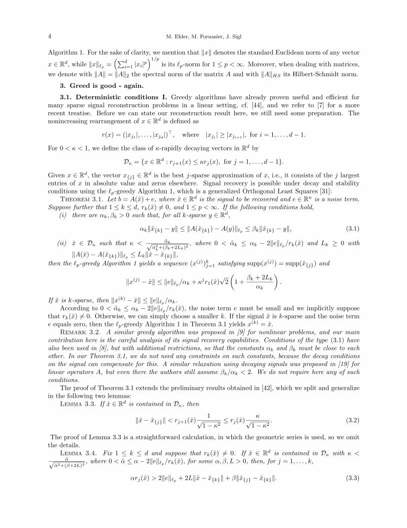
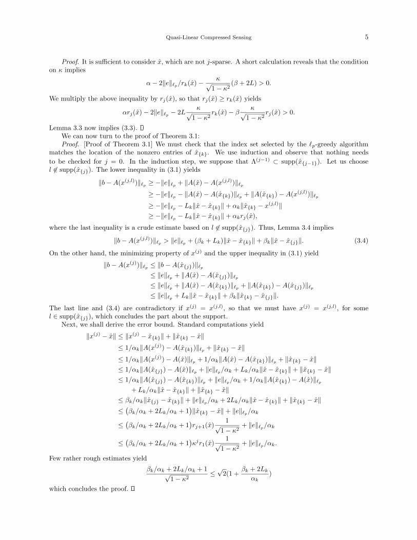
We do not claim that the model (3.6) matches all of the assumptions in Theorem 3.1, but we shallobserve that Algorithm 1 for p = 2 can be used to identify the instantaneous pulsation patterns of simulatedlight intensity data, when low frequencies are activated. This is a consequence of the fact that different lowfrequency activations result in sufficiently uncorrelated measurements in the data to be distinguished by thegreedy algorithm towards recovery. For the numerical experiments, the ambient dimension is d = 800 and wemake n = 13 measurements, see [42] for details on the choice of ωl, f , and the used multivariate optimizationroutines. We generate 2- and 3-sparse signals and apply Algorithm 1 in Figs. 1 and 2 to reconstruct thesignal. The greedy strategy identifies one additional location of the solution’s support at each iteration stepand finds the correct signal after 2 and 3 steps, respectively. In Fig. 3, we generated a signal whose entriesdecay rapidly, so that higher frequencies have lower magnitudes. We show the reconstruction of the shapeafter 3 iterations of the greedy algorithm. As expected, higher frequencies are suppressed and we obtain alow-pass filter approximation of the original shape.


(a) Original shape by means of u and the corresponding 3-sparse Fourier coefficientsx.

(b) 1-, 2-, and 3-sparse reconstruction.

Fig. 2. Original 3-sparse signal and reconstructed pulsation patterns. Red corresponds to the original signal, the recon-struction is given in blue.

(a) original shape (b) reconstructed shape

Fig. 3. The original signal is rapidly decaying with higher frequencies and we reconstruct 3 of its largest entries throughthe greedy algorithm. As desired, the reconstructed shape is a smoothened version of the original one.

3.3. Deterministic conditions II. Experiments in X-ray crystallography and diffraction imagingrequire signal reconstruction from magnitude measurements, usually in terms of light intensities. We do notpresent the explicit physical models, which would go beyond the scope of the present paper, but refer tothe literature instead. It seems impossible to provide a comprehensive list of references, so we only mention[22, 24, 29] for some classical algorithms.

Let x ∈ Rd be some signal that we need to reconstruct from measurements b =(|〈ai, x〉|2

)ni=1

, where we

selected a set of measurement vectors {ai : i = 1, . . . n} ⊂ Rd. In other words, we have phaseless measure-ments and need to reconstruct ±x. It turns out surprisingly that the above framework of reconstructionfrom nonlinear sensing can be modified to fit the phase retrieval problem. Let us stress that so far themost efficient and stable recovery procedures are based on semi-definite programming, as used in [13], by


recasting the problem into a perhaps demanding optimization on matrices. In this section we show thatthere is no need to linearize the problem by lifting the dimensionality towards low-rank matrix recovery, butis is sufficient to address a plain sparse vector recovery in the fully nonlinear setting.

In models relevant to optical measurements like diffraction imaging and X-ray crystallography, we mustdeal with the complex setting, in which x ∈ Cd is at most determined up to multiplication by a complexunit. We shall state our findings for the real case first and afterwards discuss the extensions to complexvector spaces.

3.3.1. Quasi-linear compressed sensing in phase retrieval. Let {Ai : i = 1, . . . , n} ⊂ Rd×d be acollection of measurement matrices. We consider the map

A : Rd → Rn, x 7→ A(x) = F (x)x, where F (x) =

x∗A1

...x∗An

, (3.7)

and we aim at reconstructing a signal vector x ∈ Rd from measurements b = A(x). Since A(x) = A(−x), thevector x can at best be determined up to its sign, and the lower bound in (3.1) cannot hold, not allowingus to use directly Theorem 3.1. However, we notice that for special classes of A, for instance, when{Ai : i = 1, . . . , n} are independent Gaussian matrices, the lower bound in (3.1) holds with high probabilityas long as y stays away from −x, see the heuristic probability transitions of validity of (3.1) shown in Fig. 4.Hence, there is the hope that the greedy algorithm can nevertheless be successful, because it proceeds byselecting first the largest components of the expected solution, hence orienting the reconstruction preciselytowards the direction within the space where actually (3.1) holds with high probability, in a certain senserealizing a self-fulfilling prophecy: the algorithm goes only where it is supposed to work. In order to make thisgeometric intuition more explicit we shall modify the deterministic conditions of Theorem 3.1 accordingly,so that we cover the above setting as well.

Under slightly different deterministic conditions, we derive a recovery result very similar to Theorem3.1:

Theorem 3.6. Let A be given by (3.7) and b = A(x) + e, where x ∈ Rd is the signal to be recoveredand e ∈ Rn is a noise term. Suppose further that 1 ≤ k ≤ d, rk(x) 6= 0, and 1 ≤ p < ∞. If the followingconditions are satisfied,

(i) there are constants αk, βk > 0, such that, for all k-sparse y ∈ Rd,

αk‖x{k}x∗{k} − yy∗‖HS ≤ ‖A(x{k})−A(y)‖`p ≤ βk‖x{k}x∗{k} − yy

∗‖HS , (3.8)

(ii) x ∈ Dκ with κ < αk√α2k+2(βk+2Lk)2

, where 0 < αk ≤ αk − 2‖e‖`p/rk(x) and Lk ≥ 0 with ‖A(x) −A(x{k})‖`p ≤ Lk‖xx∗ − x{k}x∗{k}‖HS,

then the `p-greedy Algorithm 1 yields a sequence (x(j))kj=1 satisfying supp(x(j)) = supp(x{j}) and

‖x(j)x(j)∗ − xx∗‖HS ≤ ‖e‖`p/αk + κjr1(x)√

3(1 +βk + 2Lk

αk).

If x is k-sparse, then ‖x(k) − x‖ ≤ ‖e‖`p/αk.Remark 3.7. Note that (3.8) resembles the restricted isometry property for rank minimization problems,

in which αk and βk are required to be close to each other, see [30, 40] and references therein. In Theorem3.6, we can allow for any pair of constants and compensate deviation between αk and βk by adding the decaycondition on the signal. In other words, we shift conditions on the measurements towards conditions on thesignal.

The structure of the proof of Theorem 3.6 is almost the same as the one for Theorem 3.1, so that wefirst derive results similar to the Lemmas 3.3 and 3.4:

Lemma 3.8. If x ∈ Rd is contained in Dκ, then

‖xx∗ − x{j}x∗{j}‖HS <√

2‖x‖rj+1(x)1√

1− κ2≤√

2‖x‖rj(x)κ√

1− κ2. (3.9)

We omit the straight-forward proof and state the second lemma that is needed:


(a) k = 2

(b) k = 3

Fig. 4. The map A is chosen as in (3.7) with independent Gaussian matrices {Ai}ni=1. We plotted the success rates of

the lower bound in (3.1) for k-sparse x ∈ Sd−1 marked in red and y running through Sd−1 with the same sparsity pattern, sothat both vectors can be visualized on a k − 1-dimensional sphere (here for k = 1, 2). Parameters are d = 80, n = 30, and αdecreases from left to right.

Lemma 3.9. Fix 1 ≤ k ≤ d and suppose that rk(x) 6= 0. If x ∈ Rd is contained in Dκ with κ <α√

α2+2(β+2L)2, where 0 < α ≤ α− 2‖e‖`p/rk(x), for some α, β, L > 0, then, for j = 1, . . . , k,

α‖x‖rj(x) > 2‖e‖`p + β‖x{j}x∗{j} − x{k}x∗{k}‖HS + 2L‖x{k}x∗{k} − xx

∗‖HS (3.10)

Proof. [Proof of Lemma 3.9] As in the proof of Lemma 3.4, the conditions on κ imply

α−2‖e‖`p‖x‖rk(x)

− κ√1− κ2

√2(β + 2L) > 0.

Multiplying by ‖x‖rj(x) and applying Lemma 3.8 yield

α‖x‖rj(x)− 2‖e‖`p − (β + 2L)‖x{j}x∗{j} − xx∗‖HS > 0.

We can further estimate

α‖x‖rj(x)− 2‖e‖`p − β‖x{j}x∗{j} − x{k}x∗{k}‖HS − 2L‖x{k}x∗{k} − xx

∗‖HS > 0,

which concludes the proof.Proof. [Proof of Theorem 3.6] As in the proof of Theorem 3.1, we must check that the index set selected

by the `p-greedy Algorithm 1 matches the location of the nonzero entries of x{k}. Again, we use induction and

the initialization j = 0 is trivial. Now, we suppose that Λ(j−1) ⊂ supp(x{j−1}) and choose l 6∈ supp(x{j}).


The lower bound in (3.8) yields

‖A(x(j,l))−A(x)‖`p ≥ ‖A(x(j,l))−A(x{k})‖`p − ‖A(x{k})−A(x)‖`p≥ αk‖x(j,l)x(j,l)∗ − x{k}x∗{k}‖HS − Lk‖x{k}x

∗{k} − xx

∗‖HS≥ α‖x{k}‖rj(x)− Lk‖x{k}x∗{k} − xx

∗‖HS ,

which is due to l 6∈ supp(x{j}), so that one row and one column of x(j,l)x(j,l)∗ corresponding to one of thej-largest entries of x are zero. Lemma 3.9 implies

‖A(x(j,l))−A(x)‖`p > 2‖e‖`p + βk‖x{j}x∗{j} − x{k}x∗{k}‖HS + Lk‖x{k}x∗{k} − xx

∗‖HS . (3.11)

On the other hand, the minimizing property of x(j) and the Condition (3.8) imply

‖A(x(j))−A(x)‖`p ≤ ‖e‖`p + ‖A(x(j))− b‖`p≤ ‖e‖`p + ‖A(x{j})− b‖`p≤ 2‖e‖`p + ‖A(x{j})−A(x{k})‖`p + ‖A(x{k})−A(x)‖`p≤ 2‖e‖`p + βk‖x{j}x∗{j} − x{k}x

∗{k}‖HS + Lk‖x{k}x∗{k} − xx

∗‖HS .

The latter inequality implies with (3.11) that x(j) = x(j,l), for all l ∈ supp(x{j}), which concludes the partabout the support.

Next, we shall verify the error bound. We obtain

‖x(j)x(j)∗ − xx∗‖HS ≤ ‖x(j)x(j)∗ − x{k}x∗{k}‖HS + ‖x{k}x∗{k} − xx∗‖HS

≤ 1/αk‖A(x(j))−A(x{k})‖`p + ‖x{k}x∗{k} − xx∗‖HS

≤ 1/αk‖A(x(j))−A(x)‖`p + 1/αk‖A(x)−A(x{k})‖`p+ ‖x{k}x∗{k} − xx

∗‖HS≤ 1/αk‖A(x{j})−A(x)‖`p + ‖e‖`p/αk + (Lk/αk + 1)‖xx∗ − x{k}x∗{k}‖HS≤ 1/αk‖A(x{j})−A(x{k})‖`p + 1/αk‖A(x{k})−A(x)‖`p + ‖e‖`p/αk

+ (Lk/αk + 1)‖xx∗ − x{k}x∗{k}‖HS≤ βk/αk‖x{j}x∗{j} − x{k}x

∗{k}‖HS + ‖e‖`p/αk

+ (2Lk/αk + 1)‖xx∗ − x{k}x∗{k}‖HS≤(βk/αk + 2Lk/αk + 1

)‖xx∗ − x{j}x∗{j}‖HS + ‖e‖`p/αk


)√2rj+1(x)

1√1− κ2

+ ‖e‖`p/αk


)κj√

2r1(x)1√

1− κ2+ ‖e‖`p/αk.

Some rough estimates yield

βk/αk + 2Lk/αk + 1√1− κ2

√2 ≤√

3(1 +βk + 2Lk

αk),

which concludes the proof.Remark 3.10. The greedy Algorithm 1 can also be performed in the complex setting. The complex

version of Theorem 3.6 also holds when recovery of ±x is replaced by a complex unit vector times x.

3.4. Signal recovery from random measurements. We aim at choosing {Ai : i = 1, . . . , n} in asuitable random way, so that the conditions in Theorem 3.6 are satisfied with high probability. Indeed, theupper bound in (3.8) is always satisfied for some C > 0, because we are in a finite-dimensional regime. Inthis section we are interested in one rank matrices Ai = aia

∗i , for some vector ai ∈ Rd, i = 1, . . . , n, because

then

A(x) =(x∗A1x, . . . , x

∗Anx)∗

= (|〈a1, x〉|2, . . . , |〈an, x〉|2)> (3.12)

models the phase retrieval problem.


3.4.1. Real random measurement vectors. To check on the assumptions in Theorem 3.6, we shalldraw at random the measurement vectors {ai : i = 1, . . . , n} from probability distributions to be charac-terized next. We say that a random vector a ∈ Rd satisfies the small-ball assumption if there is a constantc > 0, such that, for all z ∈ Rd and ε > 0,

P(|〈a, z〉| ≤ ε‖z‖

)≤ cε.

Moreover, we say that a is isotropic if E|〈a, z〉|2 = ‖z‖2, for all z ∈ Rd. The vector a is said to be L-subgaussian if, for all z ∈ Rd and t ≥ 1,

P(|〈a, z〉| ≥ tL‖z‖

)≤ 2e−t

2/2.

Eldar and Mendelson derived the following result:Theorem 3.11 ([23]). Let {ai : i = 1, . . . , n} be a set of independent copies of a random vector a ∈ Rd

that is isotropic, L-subgaussian, and satisfies the small-ball assumption. Then there are positive constantsc1, . . . , c4 such that, for all t ≥ c1 with n ≥ kc2t3 log(ed/k), and for all k-sparse x, y ∈ Rd,

n∑i=1

∣∣|〈ai, x〉|2 − |〈ai, y〉|2∣∣ ≥ c4‖x− y‖‖x+ y‖ (3.13)

with probability of failure at most 2e−kc3t2 log(ed/k).

The uniform distribution on the sphere and the Gaussian distribution on Rd induce random vectorssatisfying the assumptions of Theorem 3.11. However, at first glance, the above theorem does not help usdirectly, because we are seeking for an estimate involving the Hilbert-Schmidt norm. It is remarkable thoughthat

‖xx∗ − yy∗‖HS ≤ ‖x− y‖‖x+ y‖ ≤√

2‖xx∗ − yy∗‖HS . (3.14)

The relation (3.14) then yields that also the lower bound in (3.8) is satisfied for any constant α ≤ c4, so thatTheorem 3.6 can be used for p = 1. Thus, if the signal x is sparse and satisfies decay conditions matchingthe constants in (3.8), then Algorithm 1 for p = 1 recovers x(k) = ±x.

3.4.2. Complex random measurement vectors. In the following and at least for the uniform dis-tribution on the sphere, we shall generalize Theorem 3.11 to the complex setting, so that the assumptionsof Theorem 3.6 hold with high probability.

Theorem 3.12. If {ai : i = 1, . . . , n} are independent uniformly distributed vectors on the unit sphere,then there is a constant α > 0 such that, for all k-sparse x, y ∈ Cd and n ≥ c1k log(ed/k),

n∑i=1

∣∣|〈ai, x〉|2 − |〈ai, y〉|2∣∣ ≥ αn‖xx∗ − yy∗‖HSwith probability of failure at most e−nc2 .

Proof. For fixed x, y ∈ Rd, the results in [13] imply that there are constants c1, c > 0 such that, for allt > 0,

n∑i=1

∣∣|〈ai, x〉|2 − |〈ai, y〉|2∣∣ ≥ 1/√

(2)(c1 − t)n‖xx∗ − yy∗‖HS (3.15)

with probability of failure at most 2e−nct2

. If both x and y are k-sparse, then the union of their supportsinduces an at most 2k-dimensional coordinate subspace, so that also xx∗ − yy∗ can be reduced to a 2k× 2kmatrix, by eliminating rows and columns that do not belong to the indices of the subspace. Results in[13] can be used to derive that the estimate (3.15) holds uniformly for elements in this subspace whenn ≥ c3t

−2 log(t−1)2k, for some constant c3 > 0. There are at most(d2k

)≤ (ed/(2k))2k many of such

coordinate subspaces, see also [4]. Therefore, by a union bound, the probability of failure is at most

(ed/(2k))2k2e−nct2

= 2e−n(ct2− 2k log(ed/(2k))

n

).

Thus, if also n ≥ 1ct2−c2 log(ed/2k)2k with ct2 − c2 > 0, then we have the desired result.

Remark 3.13. We want to point out that the use of the term ‖x − y‖‖x + y‖ limits Theorem 3.11 tothe real setting. Our observation (3.14) was the key to derive the analog result in the complex setting.


3.4.3. Rank-m projectors as measurements. A slightly more general phase retrieval problem wasdiscussed in [2], where the measurement A in (3.7) is given by Ai = d

mPVi , i = 1, . . . , n, and each PVi is anorthogonal projector onto an m-dimensional linear subspace Vi of Rd. The set of all m-dimensional linearsubspaces Gm,d is a manifold endowed with the standard normalized Haar measure σm:

Theorem 3.14 ([2]). There is a constant um > 0, only depending on m, such that the following holds:for 0 < r < 1 fixed, there exist constants c(r), C(r) > 0, such that, for all n ≥ c(r)d and {Vj : j = 1, . . . n} ⊂Gm,d independently chosen random subspaces with identical distribution σm, the inequality

n∑i=1

∣∣x∗Aix− y∗Aiy∣∣ ≥ um(1− r)n‖xx∗ − yy∗‖2, (3.16)

for all x, y ∈ Rd, holds with probability of failure at most e−C(r)n. Since the rank of xx∗ − yy∗ is at most2, its Hilbert-Schmidt norm is bounded by

√2 times the operator norm. Thus, we have the lower `1-bound

in (3.8) for k = d when n ≥ c(r)d, and the random choice of subspaces (and hence orthogonal projectors)enables us to apply Theorem 3.6. The result for k-sparse signals is a consequence of Theorem 3.14:

Corollary 3.15. There is a constant um > 0, only depending on m, such that the following holds: for0 < r < 1 fixed, there exist constants c(r), C(r) > 0, such that, for all n ≥ c(r)k log(ed/k) and {Vj : j =1, . . . n} ⊂ Gm,d independently chosen random subspaces with identical distribution σm, the inequality

n∑i=1

∣∣x∗Aix− y∗Aiy∣∣ ≥ um(1− r)n‖xx∗ − yy∗‖HS , (3.17)

for all k-sparse x, y ∈ Rd, holds with probability of failure at most e−C(r)n.Proof. The lower bound on n in Theorem 3.14 is not needed when the vectors x and y are fixed in

(3.16), cf. [2]. If both x, y are supported in one fixed coordinate subspace of dimension 2k, then the proof ofTheorem 3.14 in [2], see also [13], yields that (3.17) holds uniformly for this subspace provided n ≥ c(r)2k.

Similar to the proof of Theorem 3.12, we shall use Theorem 3.14 with a 2k coordinate subspace and thenapply a union bound by counting the number of such subspaces. Indeed, since xx∗− yy∗ can be treated as a2k× 2k matrix by removing zero rows and columns, Theorem 3.14 implies (3.17) for all x, y ∈ Rd supportedin a fixed coordinate subspace of dimension 2k with probability of failure at most e−C(r)n when n ≥ c(r)2k.Again, we have used that xx∗ − yy∗ has rank at most two, so that the Hilbert-Schmidt norm is bounded by√

2 times the operator norm. The remaining part can be copied from the end of the proof of Theorem 3.12.

Remark 3.16. It is mentioned in [2] already that Theorem 3.14 also holds in the complex setting.Therefore, Corollary 3.15 has a complex version too, and our present results hold for complex rank-m pro-jectors.

3.4.4. Nearly isometric random maps. To conclude the discussion on random measurements forphase retrieval, we shall generalize some results from [40] to sparse vectors. Also, we want to present aframework, in which {Ai : i = 1, . . . , n} in (3.12) can be chosen as a set of independent random matriceswith independent Gaussian entries. Let A be a random map that takes values in linear maps from Rd×d toRn. Then A is called nearly isometrically distributed if, for all X ∈ Rd×d,

E‖A(X)‖2 = ‖X‖2HS , (3.18)

and, for all 0 < ε < 1, we have

(1− ε)‖X‖2HS ≤ ‖A(X)‖2 ≤ (1 + ε)‖X‖2HS (3.19)

with probability of failure at most 2e−nf(ε), where f : (0, 1)→ R>0 is an increasing function.Note that the definition of nearly isometries in [40] is more restrictive, but we can find several examples

there. For instance, if {Ai : i = 1, . . . , n} in (3.12) are independent matrices with independent standardGaussian entries, then the map

A : Rd×d → Rn, A(X) :=1√n

trace(A∗1X)...

trace(A∗nX)


is nearly isometrically distributed, see [17, 40].The following theorem fits into our setting, and it should be mentioned that we will only use (3.18) and

(3.19) for symmetric matrices X of rank at most 2. So, we could even further weaken the notion of nearlyisometric distributions accordingly.

Theorem 3.17. Fix 1 ≤ k ≤ d. If A is a nearly isometric random map from Rd×d to Rn andA(x) := A(xx∗), then there are constants c1, c2 > 0, such that, uniformly for all 0 < δ < 1 and all k-sparsex, y ∈ Rd,

(1− δ)‖xx∗ − yy∗‖HS ≤ ‖A(x)−A(y)‖ ≤ (1 + δ)‖xx∗ − yy∗‖HS (3.20)

with probability of failure at most 2e−n(f(δ/2)− 4k+2

n log(65/δ)− 2kn log(ed/2k)

).

As a consequence of Theorem 3.17, we can fix δ and derive two constants c1, c2 > 0 depending only on δand f(δ/2), such that (3.20) holds for all k-sparse x, y ∈ Rd in a uniform fashion with probability of failureat most e−c1n whenever n ≥ c2k log(ed/k). The analogous result for not necessarily sparse vectors is derivedin [40].

Proof. We fix an index set I of 2k coordinates in Rd, denote the underlying coordinate subspace by V ,and define

X = {X ∈ Rd×d : X = X∗, rank(X) ≤ 2, ‖X‖HS = 1, Xi,j = 0, if i 6∈ I or j 6∈ I}.

Any element X ∈ X can be written as X = axx∗ + byy∗ such that a2 + b2 = 1 and x, y ∈ V are orthogonalunit norm vectors. In order to build a covering of X , we start with a covering of the 2k-dimensional unitsphere SV in V . Indeed, there is a finite set N1 ⊂ SV of cardinality at most (1+ 64

δ )2k ≤ ( 65δ )2k, such that, for

every x ∈ SV , there is y ∈ N1 with ‖x−y‖ ≤ δ/32, see, for instance, [45, Lemma 5.2]. We can also uniformlycover [−1, 1] with a finite set of cardinality 32

δ , so that the error is bounded by δ/16. Thus, we can coverX with a set N of cardinality at most ( 32

δ )2( 65δ )4k ≤ ( 65

δ )4k+2, such that, for every X = axx∗ + byy∗ ∈ X ,there is Y = a0x0x0 + b0y0y

∗0 ∈ N with

|a− a0| ≤ δ/16, |b− b0| ≤ δ/16, ‖x− x0‖ ≤ δ/32, ‖y − y0‖ ≤ δ/32. (3.21)

We can choose ε = δ/2, so that (3.19) holds uniformly onN with probability of failure at most 2( 65δ )4k+2e−nf(δ/2).

Taking the square root yields with at most the same probability of failure that

1− δ/2 ≤ ‖A(Y )‖ ≤ 1 + δ/2

holds uniformly for all Y ∈ N .We now define the random variable

M = max{K ≥ 0 : ‖A(X)‖ ≤ K‖X‖HS , for all X ∈ X} (3.22)

and consider an arbitrary X = axx+ byy∗ ∈ X . Then there is Y = a0x0x0 + b0y0y∗0 ∈ N such that (3.21) is

satisfied, so that we can further estimate

‖A(X)‖ ≤ ‖A(Y )‖+ ‖A(axx+ byy∗ − a0x0x0 − b0y0y∗0)‖

≤ 1 + δ/2 + ‖A(axx− a0x0x∗0)‖+ ‖A(byy − b0y0y

∗0)‖.

Although axx − a0x0x∗0 and byy − b0y0y

∗0 may not be elements in X , a simple normalization allows us to

apply the bound (3.22), so that we obtain

‖A(X)‖ ≤ 1 + δ/2 +M‖axx− a0x0x∗0‖HS +M‖byy − b0y0y

∗0‖HS

≤ 1 + δ/2 +M |a|‖xx∗ − x0x∗0‖HS +M |a− a0|‖x0x

∗0‖HS+

M |b|‖yy∗ − y0y∗0‖HS +M |b− b0|‖y0y

∗0‖HS

≤ 1 + δ/2 +Mδ/4.

For the last inequality, we have used (3.14). By choosing X ∈ X with ‖A(X)‖ = M , we derive M ≤1 + δ/2 +Mδ/4, which implies M ≤ 1 + δ. Thus, we obtain ‖A(X)‖ ≤ 1 + δ.


(a) d = 20, n = 7 (b) d = 20, n = 11

Fig. 5. Signal reconstruction rates vs. sparsity k. Reconstruction is repeated 50 times for each signal and k to derivestable recovery rates. For small k, we almost certainly recover the signal, and, as expected, increasing k leads to decreasedsuccess rates.

The lower bound is similarly derived by

‖A(X)‖ ≥ ‖A(Y )‖ − ‖A(Y −X)‖ ≥ 1− δ/2− (1 + δ)δ/4 ≥ 1− δ.

So far, we have the estimate (3.20) in a uniform fashion for all x, y in some fixed coordinate subspaceof dimension 2k with probability of failure at most 2( 65

δ )4k+2e−nf(δ/2). Again, we derive the union boundby counting subspaces as in the proof of Theorem 3.12. There are at most (ed/(2k))2k many subspaces, sothat we can conclude the proof.

3.5. Numerical experiments for greedy phase retrieval. We shall follow the model in (3.12) andstudy signal reconstruction rates for random choices of measurement vectors {ai : i = 1, . . . n} chosen asindependent standard Gaussian vectors. For a fixed number of measurements n, we shall study the signalrecovery rate depending on the sparsity k. We expect to have high success rates for small k and decreasedrates when k grows. Figure 5 shows results of numerical experiments consistent with our theoretical findings.We must point out though that each step of the greedy algorithm requires solving a nonconvex globaloptimization problem. Here, we used standard optimization routines that may yield results that are notoptimal. Better outcomes can be expected when applying more sophisticated global optimization methods,for instance, based on adaptive grids and more elaborate analysis of functions of few parameters in highdimensions, cf. [16].

4. Iterative thresholding for quasi-linear problems. Although the quasi-linear structure of themeasurements does not play an explicit role in the formulation of Algorithm 1, in the examples we showed inthe previous sections it was nevertheless a crucial aspect to obtain generalized RIP conditions such as (3.1)and (3.8). When using iterative thresholding algorithms, as we shall show below, the quasi-linear structureof the measurements gets into the formulation of the algorithms as well. Hence, from now on we shall be abit more explicit on the form of nonlinearity and we consider a map F : Rd → Rn×d, and aim to reconstructx ∈ Rd from measurements b ∈ Rn given by

F (x)x = b.

As guiding examples, we keep as references the maps A in Proposition 3.5, which can be written asA(x) = F (x)x, where F (x) = A1 + εf(‖x− x0‖)A2.

The study of iterative thresholding algorithms that we propose below is motivated by the intrinsiclimitations of Algorithm 1, in particular, its restriction to recovering only signals which have a rapid decayof their nonincreasing rearrangement, and the potential complexity explosion due to the need of performingseveral high-dimensional global optimizations at each greedy step.


4.1. Iterative hard-thresholding. We follow ideas in [8] and aim to use the iterative scheme

x(j+1) :=(x(j) +

1

µkF (x(j))∗(b− F (x(j))x(j))

){k}, (4.1)

where µk > 0 is some parameter and, as before, y{k} denotes the best k-sparse approximation of y ∈ Rd.The following theorem is a reformulation of a result by Blumensath in [8]:

Theorem 4.1. Let b = A(x) + e, where x ∈ Rd is the signal to be recovered and e ∈ Rn is a noise term.Suppose 1 ≤ k ≤ d is fixed. If F satisfies the following assumptions,

(i) there is c > 0 such that ‖F (x)‖2 ≤ c,(ii) there are αk, βk > 0 such that, for all k-sparse x, y, z ∈ Rd,

αk‖x− y‖ ≤ ‖F (z)(x− y)‖ ≤ βk‖x− y‖, (4.2)

(iii) there is Ck > 0 such that, for all k-sparse y ∈ Rd,

‖F (x{k})− F (y)‖2 ≤ Ck‖x{k} − y‖, (4.3)

(iv) there is Lk > 0 such that ‖F (x)x− F (x{k})x{k}‖ ≤ Lk‖x− x{k}‖,(v) the constants satisfy β2

k ≤ 1/µk <32α

2k − 4‖x{k}‖2C2

k ,then the iterative scheme (4.1) converges towards x? satisfying

‖x? − x‖ ≤ γ‖e‖+ (1 + γc+ γLk)‖x− x{k}‖,

where γ = 20.75α2

k−1/µk−2‖x{k}‖2C2k

.

Note that (4.2) is again a RIP condition for each F (z). The proof of Theorem 4.1 is based on Blumen-sath’s findings in [8], where the nonlinear operator A is replaced by its first order approximation at x(j)

within the iterative scheme. When dealing with the quasi-linear setting, it is natural to use F (x(j)), so weformulated the iteration in this way already.

Proof. We first verify that the assumptions in [8, Corollary 2] are satisfied. By using (4.3), we derive,for k-sparse y ∈ Rd,

‖F (x{k})x{k} − F (y)y − F (y)(x{k} − y)‖ = ‖F (x{k})x{k} − F (y)x{k}‖≤ ‖x{k}‖Ck‖x{k} − y‖.

The assumptions of [8, Corollary 2] are satisfied, which implies that the iterative scheme (4.1) converges tosome k-sparse x? satisfying

‖x? − x‖ ≤ γ‖b− F (x{k})x{k}‖+ ‖x{k} − x‖,

where γ = 20.75α2

k−1/µk−2‖x{k}‖2C2k

. We still need to estimate the left term on the right-hand side. A zero

addition yields

‖b− F (x{k})x{k}‖ ≤ ‖e‖+ ‖F (x)x− F (x{k})x{k}‖≤ ‖e‖+ Lk‖x− x{k}‖,

which concludes the proof.We shall verify that the map in Proposition 3.5 satisfies the assumptions of Theorem 4.1 at least when

x is k-sparse:Example 4.2. Let F (x) = A1 + εf(‖x − x0‖)A2, so that F (x)x = A(x) with A as in Proposition

3.5. By a similar proof and under the same notations we derive that an upper bound in (4.2) can bechosen as β = 1 + δ + εB‖A2‖, where δ is the RIP constant for A1. For the lower bound, we computeα = 1− δ − εB‖A2‖. In other words, F (x) satisfies the RIP of order k with constant δ + εB‖A2‖. In (4.3),we can choose C = εL‖A2‖. Thus, if ε, B, ‖A2‖, δ are sufficiently small, then the assumptions of Theorem4.1 are satisfied.


4.2. Iterative soft-thresholding. The type of thresholding in the scheme (4.1) of the previous sectionis one among many potential choices. Here, we shall discuss soft-thresholding, which is widely applied whendealing with linear compressed sensing problems. Our findings in this section are based on preliminary resultsin [42]. We suppose that the original signal is sparse and, in fact, we aim to reconstruct the sparsest x thatmatches the data b = F (x)x. In other words, we intend to solve for x ∈ Rd with x = arg min ‖x‖`0 subjectto F (x)x = b. Theorem 4.1 yields that we can use iterative hard-thresholding to reconstruct the sparsestsolution. Here, we shall follow a slightly different strategy. As `0-minimization is a combinatorial optimiza-tion problem and computationally cumbersome in principle, even NP-hard under many circumstances, it iscommon practice in compressed sensing to replace the `0-pseudo norm with the `1-norm, so that we considerthe problem

arg min ‖x‖`1 subject to F (x)x = b. (4.4)

It is also somewhat standard to work with an additional relaxation of it and instead solve for xα given by

xα := arg minx∈Rd

Jα(x), where Jα(x) := ‖F (x)x− b‖2`2 + α‖x‖`1 , (4.5)

where α > 0 is sometimes called the relaxation parameter. The optimization (4.5) allows for F (x)x 6= b,hence, is particularly beneficial when we deal with measurement noise, so that b = F (x)x+ e and α can besuitably chosen to compensate for the magnitude of e. If there is no noise term, then (4.5) approximates(4.4) when α tends to zero. The latter is a standard result but we explicitly state this and prove it for thesake of completeness:

Proposition 4.3. Let the map x 7→ F (x) be continuous and suppose that (αn)∞n=1 is a sequence ofnonnegative numbers that converge towards 0. If (xαn)∞n=1 is any sequence of minimizers of Jαn , then itcontains a subsequence that converges towards a minimizer of (4.4). If the minimizer of (4.4) is unique,then the entire sequence (xαn)∞n=1 converges towards this minimizer.

Proof. Let x be a minimizer of (4.4). Direct computations yield

‖xαn‖`1 ≤1

αnJαn(xαn) ≤ 1

αnJαn(x) = ‖x‖`1 . (4.6)

Thus, there is a convergent subsequence (xαnj )∞j=1 → x ∈ Rd, for j →∞. Since

‖F (x)x− y‖ = limj→∞

‖F (xαnj )xαnj − y‖ ≤ limj→∞

Jαnj (xαnj ) ≤ limj→∞

Jαnj (x) = 0

and (4.6) hold, x must be a minimizer of (4.4).Now, suppose that the minimizer x of (4.4) is unique. If x0 is an accumulation point of (xαn)∞j=1, then

there is a subsequence converging towards x0. The same arguments as above with the uniqueness assumptionyield x0 = x, so that (xαn)∞j=1 is a bounded sequence with only one single accumulation point. Hence, theentire sequence converges towards x. From here on, we shall focus on (4.5), which we aim to solve at leastapproximately using some iterative scheme. First, we define the map

Sα : Rd → Rd, x 7→ Sα(x) := arg miny∈Rd

‖F (x)y − b‖2 + α‖y‖`1 .

To develop the iterative scheme, we present some conditions, so that Sα is contractive:Theorem 4.4. Given b ∈ Rn, fix α > 0 and suppose that there are constants c1, c2, c3, γ > 0 such that,

for all x, y ∈ Rd,(i) ‖F (x)‖2 ≤ c1,

(ii) there is zx ∈ Rd such that ‖zx‖`1 ≤ c2‖b‖ and F (x)zx = b,(iii) ‖F (x)− F (y)‖2 ≤ c3‖x− y‖,(iv) if y is 4

α2 (c1 + c2 + c21c2)2‖b‖2-sparse, then

(1− γ)‖y‖2 ≤ ‖F (x)y‖2 ≤ (1 + γ)‖y‖2,

(v) the constants satisfy γ < 1− (1 + 2c1c2)c3‖b‖,


then Sα is a bounded contraction, so that the recursive scheme x(j+1)α := Sα(x

(j)α ) converges for any initial

vector towards a point xα satisfying the fixed point relationship

xα = arg miny∈Rd

‖F (xα)y − b‖2 + α‖y‖`1 . (4.7)

Remark 4.5. We believe that the fixed point of (4.7) in Theorem 4.4 is close to the actual minimizerof (4.5). To support this point of view, we shall later investigate on the distance ‖xα − xα‖ in Theorem 4.8and also provide some numerical experiments in Section 4.3.

A few more comments are in order before we take care of the proof: Note that the constant c1 must holdfor the operator norm in (i), and γ in the RIP of (iv) covers only sparse vectors. Therefore, 1 + γ can bemuch smaller than c1. Condition (iii) is a standard Lipschitz property. If γ is indeed less than 1, then smalldata b can make up for larger other constants, so that (v) can hold. The requirement (ii) is more delicatethough and a rough derivation goes as follows: the data b are supposed to lie in the range of F (x), whichis satisfied, for instance, if F (x) is onto. The pseudo-inverse of F (x) then yields a vector zx with minimal`2-norm. We can then ask for boundedness of all operator norms of the pseudo-inverses. However, we stillneed to bound the `1-norm by using the `2-norm, which introduces an additional factor

√d.

We introduce the soft-thresholding operator Sα : Rd → Rd, x 7→ Sα(x) given by

(Sα(x))i =

xi − α/2, α/2 ≤ xi0, −α/2 < xi < α/2

xi + α/2, xi ≤ −α/2, (4.8)

which we shall use in the following proof:Proof. [Proof of Theorem 4.4] For x ∈ Rd, we can apply (ii), so that F (x)zx = b and ‖zx‖`1 ≤ c2‖b‖,

implying

α‖Sα(x)‖ ≤ ‖F (x)Sα(x)− b‖2 + α‖Sα(x)‖`1 ≤ α‖zx‖`1 ≤ αc2‖b‖.

Thus, we have ‖Sα(x)‖ ≤ c2‖b‖.The conditions (i) and (iii) imply

‖F (x)∗F (x)− F (y)∗F (y)‖ ≤ 2c1c3‖x− y‖. (4.9)

It is well-known that

Sα(x) = Sα(ξ(x)

), where ξ(x) = (I − F (x)∗F (x)))Sα(x) + F (x)∗b, (4.10)

and Sα is the soft-thresholding operator in (4.8), cf. [18]. Note that ξ can be bounded by

‖ξ(x)‖ = ‖(I − F (x)∗F (x))Sα(x)‖+ ‖F (x)∗b‖≤ c2‖b‖+ c21c2‖b‖+ c1‖b‖= (c1 + c2 + c21c2)‖b‖.

It is known, cf. [20] and [25, Lemma 4.15], that the bound on ξ implies

# supp(Sα(x)

)= # supp

(Sα(ξ(x))

)≤ 4

α2(c1 + c2 + c21c2)2‖b‖2.

The condition (iv) can be rewritten as ‖(I − F (x)∗F (x))y‖ ≤ γ‖y‖, for suitably sparse y. Since soft-thresholding is nonexpansive, i.e.,

‖Sα(x)− Sα(y)‖ ≤ ‖x− y‖,

the identity (4.10) then yields with (4.9)

‖Sα(x)−Sα(y)‖ ≤ ‖Sα(x)−Sα(y) + F (x)∗b− F (y)∗b

− F (x)∗F (x)Sα(x) + F (y)∗F (y)Sα(y)‖≤ ‖(I − F (x)∗F (x))(Sα(x)−Sα(y))‖

+ ‖(F (y)∗F (y)− F (x)∗F (x))Sα(y)‖+ ‖(F (x)∗ − F (y)∗)b‖≤ γ‖Sα(x)−Sα(y)‖+ 2c1c2c3‖b‖‖x− y‖+ c3‖x− y‖‖b‖,


which implies

‖Sα(x)−Sα(y)‖ ≤ 2c1c2 + 1

1− γc3‖b‖‖x− y‖.

Thus, Sα is contractive and x(j)α converges towards a fixed point. If ‖b‖ is large, then the conditions in

Theorem 4.4 are extremely strong. For smaller ‖b‖, on the other hand, we can find examples matching therequirements. Note also that the above proof reveals that xα is at most d 4

α2 (c1 + c2c4)2‖b‖2e-sparse.Example 4.6. As in Example 4.2, let F (x) = A1 + εf(‖x − x0‖)A2, so that F (x)x = A(x) with A as

in Proposition 3.5. We additionally suppose that n ≤ d, that A1 is onto, and denote the smallest eigenvalueof A1A

∗1 by β > 0. Then we can choose c1 = ‖A1‖ + εB‖A2‖2 and c3 = εL‖A2‖. If ε, B, ‖A2‖ are

sufficiently small, then the smallest eigenvalue of F (x)F (x)∗ is almost given by the smallest eigenvalue ofA1A

∗1 and denoted by β > 0. If F (x)† = F (x)∗(F (x)F (x)∗)−1 denotes the pseudo-inverse of F (x), then

‖F (x)†‖2 ≤ c1/β. For (ii), we can define y := F (x)†b, so that ‖y‖`1 ≤√d‖y‖ ≤

√d c1β ‖b‖ and c2 ≤

√d c1β .

Still, suppose that ε, B, ‖A2‖ are sufficiently small and also assume that A1 satisfies the RIP with constant0 < δ < 1 for sufficiently large sparsity requirements in (iv). Thus, the conditions of Theorem 4.4 aresatisfied if ‖b‖ is sufficiently small.

Quasi-linear iterative soft-thresholding:Input: F : Rd → Rn×d, b ∈ RnInitialize x(0) as an arbitrary vectorfor j = 0, 1, 2, . . . until some stopping criterion is met do

x(j+1)α := arg min

x∈RdJ Sα (x, x(j)

α ) = Sα((I − F (x(j)

α )∗F (x(j)α ))x(j)

α + F (x(j)α )∗b

)end

Output: x(1)α , x

(2)α , . . .

Algorithm 2: We propose to iteratively minimize the surrogate functional, which yields a simpleiterative soft-thresholding scheme.

The recursive scheme in Theorem 4.4 involving Sα requires a minimization in each iteration step. Toderive a more efficient scheme, we consider the surrogate functional

J Sα (x, a) = ‖F (a)x− b‖2 + α‖x‖`1 + ‖x− a‖2 − ‖F (a)x− F (a)a‖2.

We have J Sα (x, x) = Jα(x) and propose the iterative Algorithm 2. In each iteration step, we minimize thesurrogate functional in the first variable having the second one fixed with the previous iteration, which onlyrequires a simple soft-thresholding.

Indeed, iterative soft-thresholding converges towards the fixed point xα:Theorem 4.7. Suppose that the assumptions of Theorem 4.4 are satisfied and let xα be the k-sparse

fixed point in (4.7). We define zα := (I − F (xα)∗F (xα))xα) + F (xα)∗b and K = 4‖xα‖2α2 + 4c

α C, where

C = sup1≤l<d(√l + 1‖zα − (zα){l}‖`2) and c > 0 sufficiently large. Additionally assume that

(a) there is 0 < γ < γ such that, for all K + k-sparse vectors y ∈ Rd,

(1− γ)‖y‖2‖F (xα)y‖2 ≤ (1 + γ)‖y‖2, (4.11)

(b) the constants satisfy γ + (1 + 4c1c2)c3‖b‖ < γ.

Then by using x(0)α = 0 as initial vector, the iterative Algorithm 2 converges towards xα with

‖x(j)α − xα‖ ≤ γj‖xα‖, j = 0, 1, 2, . . . .

Note that the above k is at most d 4α2 (c1 + c2 + c21c2)2‖b‖2e. Also, it may be possible to choose γ a little

bigger than necessary to ensure γ < γ. Condition (b) can then be satisfied when the magnitude of the data


b is sufficiently small. Moreover, if constants are suitably chosen, Example 4.6 also provides a map F thatsatisfies the assumptions of Theorem 4.7 when ‖b‖ is small.

Proof. We use induction and observe that the case j = 0 is trivially verified. Next, we suppose that

x(j)α satisfies ‖x(j)

α − xα‖ ≤ γj‖xα‖ and that it has at most K nonzero entries. Our aim is now to verify that

x(j+1) also satisfies the support condition and ‖x(j+1)α − xα‖ ≤ γj+1‖xα‖. To simplify notation let

f(x, y) := (I − F (x)∗F (x))y + F (x)∗b, (4.12)

so that zα = f(xα, xα). It will be useful later to derive bounds for both terms ‖f(xα, xα)− f(xα, x(j)α )‖ and

‖f(x(j)α , x

(j)α )− f(x

(j)α , x

(j)α )‖. Therefore, we start to estimate

‖f(xα, xα)− f(xα, x(j)α )‖ = ‖(I − F (xα)∗F (xα))(xα − x(j)

α )‖ ≤ γγj‖xα‖, (4.13)

where we have used (a) in the form ‖(I − F (xα)∗F (xα))y‖ ≤ γ‖y‖ and the induction hypothesis.

Next, we take care of ‖f(xα, x(j)α )− f(x

(j)α , x

(j)α )‖ and derive

‖f(xα, x(j)α )− f(x(j)

α , x(j)α )‖ ≤ ‖(F (xα)∗ − F (x(j)

α )∗)b‖+ ‖(F (x(j)

α )∗F (x(j)α )− F (xα)∗F (xα))x(j)

α ‖≤ c3γj‖xα‖‖b‖+ ‖(F (x(j)

α )∗F (x(j)α )− F (x(j)

α )∗F (xα))x(j)α ‖

+ ‖(F (x(j)α )∗F (xα)− F (xα)∗F (xα))x(j)

α ‖≤ c3γj‖xα‖‖b‖+ 2c1c3γ

j‖xα‖‖x(j)α ‖

= γj‖xα‖c3(‖b‖+ 2c1‖x(j)

α ‖).

By using (ii) and the minimizing property of xα, we derive

‖xα‖ ≤ ‖xα‖`1 ≤ ‖zxα‖`1 ≤ c2‖b‖.

The triangular inequality then yields ‖x(j)α ‖ ≤ γjc2‖b‖+ c2‖b‖. Thus, we obtain the estimate

‖f(xα, x(j)α )− f(x(j)

α , x(j)α )‖ ≤ γj‖xα‖c3‖b‖

(1 + 2c1c2(1 + γj)

). (4.14)

According to (4.13) and (4.14), the condition (b) yields

‖zα − f(x(j)α , x(j)

α )‖ ≤ γj‖xα‖(γ + c3‖b‖(1 + 2c1c2(1 + γj))) ≤ γj+1‖xα‖. (4.15)

Results in [25, Lemma 4.15] with x(j+1)α = Sα(f(x

(j)α , x

(j)α )) imply that there is a constant c > 0 such that

# supp(x(j+1)α ) ≤ 4γ2j+2‖xα‖2

α2+

4c

αC,

where C = sup1≤l<d(√l + 1‖zα − (zα){l}‖`2). Since the above right-hand side is smaller than K, we have

the desired support estimate.Next, we take care of the error bounds. Since xα is a fixed point of (4.7), we have xα = Sα(zα), which

we have already used in (4.10). The nonexpansiveness of Sα yields with zα = f(xα, xα)

‖xα − x(j+1)α ‖ ≤ ‖Sα(f(xα, xα))− Sα(f(xα, x

(j)α ))‖+ ‖Sα(f(xα, x

(j)α ))− Sα(f(x(j)

α , x(j)α ))‖

≤ ‖f(xα, xα)− f(xα, x(j)α )‖+ ‖f(xα, x

(j)α )− f(x(j)

α , x(j)α )‖.

The same way as for (4.15), we use the bounds in (4.13) and (4.14) with (b) to derive

‖xα − x(j+1)α ‖ ≤ γj‖xα‖(γ + c3‖b‖(1 + 4c1c2)) ≤ γj+1‖xα‖,

so that we can conclude the proof.It remains to verify that the output xα of the iterative soft-thresholding scheme is close to the minimizer

xα of (4.5):


Theorem 4.8. Suppose that the assumptions of Theorem 4.7 hold, that there is a K-sparse minimizerxα of (4.5), and that c2c3√

1−γ ‖b‖ < 1 holds, then we have

‖xα − xα‖ ≤√αc2‖b‖a

+c1 + c3‖x‖

a‖xα − x‖,

where x satisfies F (x)x = b and a =√

1− γ− c2c3‖b‖. Note that Proposition 4.3 yields that the minimizerxα can approximate x, so that ‖xα − x‖ can become small and, hence, ‖xα − xα‖ must be small. It shouldbe mentioned though that the assumptions of Theorem 4.7 depend on α because its magnitude steers thesparsity of xα. Therefore, letting α tend to zero is quite delicate because the assumptions become stronger.Indeed, taking the limit requires that condition (iv) in Theorem 4.4 holds for all y ∈ Rd, not just for sparsevectors, and the same is required for condition (a) in Theorem 4.7.

Proof. [Proof of Theorem 4.8] We first bound xα by

α‖xα‖ ≤ ‖F (xα)xα − b‖2 + α‖xα‖`1 ≤ ‖F (xα)xα − b‖2 + α‖xα‖ ≤ α‖zxα‖`1 .

Therefore, we have ‖xα‖ ≤ c2‖b‖. Since xα is K-sparse, we derive

‖F (xα)xα − F (xα)xα‖ ≥ ‖F (xα)xα − F (xα)xα‖ − ‖F (xα)xα − F (xα)xα‖

≥√

1− γ‖xα − xα‖ − c3‖xα − xα‖‖xα‖.

These computations and a zero addition imply

‖xα − xα‖ ≤1

a‖F (xα)xα − F (xα)xα‖

≤ 1

a(‖F (xα)xα − b‖+ ‖F (xα)xα − b‖).

We shall now bound both terms on the right-hand side separately. The minimizing property and (ii) inTheorem 4.4 yield

‖F (xα)xα − b‖2 ≤ α‖zxα‖`1 − α‖xα‖`1 ≤ αc2‖b‖.

The second term is bounded by

‖F (xα)xα − b‖ ≤ ‖F (xα)xα − F (xα)x‖+ ‖F (xα)x− F (x)x‖≤ c1‖xα − x‖+ c3‖x‖‖xα − x‖= (c1 + c3‖x‖)‖xα − x‖,

so that we can conclude the proof. Alternatively, we can also bound the distance between xα and x:Proposition 4.9. Suppose that the assumptions of Theorem 4.7 hold, that we can replace xα in condi-

tion (a) of the latter theorem with some K-sparse x ∈ Rd satisfying F (x)x = b, and that c2c3√1−γ ‖b‖ < 1 holds,

then we have

‖xα − x‖ ≤√αc2‖b‖√

1− γ − c2c3‖b‖.

Proof. We can estimate

‖xα − x‖ ≤1√

1− γ‖F (x)xα − F (x)x‖

≤ 1√1− γ

(‖F (x)xα − F (xα)xα‖+ ‖F (xα)xα − F (x)x‖

)≤ 1√

1− γ(c3‖xα‖‖xα − x‖+

√‖F (xα)xα − b‖2 + α‖xα‖`1

)≤ 1√

1− γ(c3c2‖b‖‖xα − x‖+

√α‖zxα‖`1

)≤ 1√

1− γ(c3c2‖b‖‖xα − x‖+

√αc2‖b‖

).

From here on, some straight-forward calculations yield the required statement.


(a) iterative soft-thresholding (b) iterative hard-thresholding

Fig. 6. Recovery rates for iterative hard- and soft-thresholding used with the measurements in the Examples 4.2 and 4.6with d = 80, n = 20, A1 having i.i.d. Gaussian entries, ε = 1, and A2 = I. The sparsity parameter k runs on the horizontalaxis from 1 to 10, the norm of x runs on the vertical axis from 0.01 to 1. As expected, the recovery rates decrease withgrowing k. Consistent with the theory, we also observe decreased recovery rates for larger signal norms with soft-thresholding.Hard-thresholding appears only successful for these parameters when k = 1, but throughout the entire range of considered signalnorms.

4.3. Numerical experiments for iterative thresholding. Theorem 4.7 provides a simple thresh-olding algorithm to compute the fixed point xα in (4.7) that is more efficient than the recursive scheme inTheorem 4.4. To support Theorem 4.8, we shall check numerically that xα is indeed close to a minimizer xαof (4.5).

The quasi-linear measurements are taken from the Examples 4.2 and 4.6. The recovery rates fromiterative hard- and soft-thresholding are plotted in Figure 6(a) and show a phase transition. For soft-thresholding, this transition depends on both, the sparsity level k and the measurement magnitude. Thoseobservations are consistent with the theoretical results in Theorem 4.7 und suggest that the original signalcan be recovered by iterative soft-thresholding. We also use hard-thresholding but for comparable parameterchoices the signal was only recovered when k = 1, cf. Fig. 6(b).

The assumptions of the Theorems 4.1 and 4.7 cannot be satisfied within the phase retrieval setting, and

the initial vectors x(0) = x(0)α = 0 in (4.1) and in Algorithm 2, respectively, would lead to a sequence of zero

vectors. We observed numerically, that other choices of initial vectors do not yield acceptable recovery rateseither, so that we did not pursue this direction.

Acknowledgments. Martin Ehler acknowledges the financial support by the Research Career Tran-sition Awards Program EH 405/1-1/575910 of the National Institutes of Health and the German ScienceFoundation. Massimo Fornasier is supported by the ERC-Starting Grant for the project “High-DimensionalSparse Optimal Control”. Juliane Sigl acknowledges the partial financial support of the START-Project“Sparse Approximation and Optimization in High-Dimensions” and the hospitality of the Johann Radon In-stitute for Computational and Applied Mathematics, Austrian Academy of Sciences, Linz, during the earlypreparation of this work.

REFERENCES

[1] C. Aerts, J. Christensen-Dalsgaard, and D. W. Kurtz, Asteroseismology, Springer, Berlin, 2010.[2] C. Bachoc and M. Ehler, Signal reconstruction from the magnitude of subspace components, arXiv:1209.5986, (2012).[3] B. Bah and J. Tanner, Improved bounds on restricted isometry constants for gaussian matrices, SIAM J. Matrix Anal.,

31 (2010), pp. 2882–2898.[4] R. Baraniuk, M. Davenport, R. DeVore, and M. Wakin, A simple proof of the restricted isometry property for random

matrices, Constr. Approx., 28 (2008), pp. 253–263.[5] F. Barning, The numerical analysis of the light-curve of 12 lacertae, Bulletin of the Astronomical Institutes of the

Netherlands, 17 (1963), pp. 22–28.[6] H. H. Bauschke, P. L. Combettes, and D. R. Luke, Phase retrieval, error reduction algorithm, and Fienup variants:

A view from convex optimization, J. Opt. Soc. Amer. A, 19 (2002), pp. 1334–1345.[7] J. D. Blanchard, C. Cartis, J. Tanner, and A. Thompson, Phase transitions for greedy sparse approximation algo-

rithms, Appl. Comput. Harmon. Anal., 30 (2011), pp. 188–203.


[8] T. Blumensath, Compressed sensing with nonlinear observations and related nonlinear optimisation problems,arXiv:1205.1650v1, (2012).

[9] T. Blumensath and M. E. Davies, Gradient pursuit for non-linear sparse signal modelling, Proc. European SignalProcessing Conference (EUSIPCO), (2008).

[10] , Iterative hard thresholding for compressed sensing, Appl. Comput. Harmon. Anal., 27 (2009), pp. 265–274.[11] E. J. Candes, J. Romberg, and T. Tao, Robust uncertainty principles: Exact signal reconstruction from highly incom-

plete frequency information, IEEE Trans. Inform. Theory, 52 (2006), pp. 489–509.[12] E. J. Candes, J. Romberg, and T. Tao, Stable signal recovery from incomplete and inaccurate measurements,

Comm. Pure Appl. Math., 59 (2006), pp. 1207–1223.[13] E. J. Candes, T. Strohmer, and V. Voroninski, PhaseLift: Exact and stable signal recovery from magnitude mea-

surements via convex programming, Communications on Pure and Applied Mathematics, DOI:10.1002/cpa.21432,(2012).

[14] E. J. Candes and T. Tao, Decoding by linear programming, IEEE Trans. Inform. Theory, 51 (2005), pp. 4203–4215.[15] , Near-optimal signal recovery from random projections: universal encoding strategies, IEEE Trans. Inform. Theory,

52 (2006), pp. 5406–5425.[16] A. Cohen, R. A. DeVore, G. Petrova, and P. Wojtaszczyk, Finding the minimum of a function, preprint, (2013).[17] S. Dasgupta and A. Gupta, An elementary proof of a theorem of Johnson and Lindenstrauss, Random Structures &

Algorithms, 22 (2003), pp. 60–65.[18] I. Daubechies, M. Defrise, and C. DeMol, An iterative thresholding algorithm for linear inverse problems with a

sparsity constraint, Comm. Pure Appl. Math., 57 (2004), pp. 1413–1541.[19] M. A. Davenport and M. B. Wakin, Analysis of orthogonal matching pursuit using the restricted isometry property,

IEEE Trans. Inform. Theory, 56 (2010), pp. 4395–4401.[20] R. A. DeVore, Nonlinear approximation, Acta Numerica, (1998), pp. 51–150.[21] D. L. Donoho, Compressed sensing, IEEE Trans. Inform. Theory, 52 (2006), pp. 1289–1306.[22] J. Drenth, Principles of Protein X-Ray Crystallography, Springer, 2010.[23] Y. C. Eldar and S. Mendelson, Phase retrieval: Stability and recovery guarantees, arXiv:1211.0872, (2012).[24] J. R. Fienup, Phase retrieval algorithms: a comparison, Applied Optics, 21 (1982), pp. 2758–2769.[25] M. Fornasier, ed., Theoretical Foundations and Numerical Methods for Sparse Recovery, vol. 9 of Radon Series on

Computational and Applied Mathematics, De Gruyter, 2010.[26] M. Fornasier and H. Rauhut, Iterative thresholding algorithms, Appl. Comput. Harmon. Anal, 25 (2008), pp. 187–208.[27] , Recovery algorithms for vector valued data with joint sparsity constraints, SIAM J. Numer. Anal., 46 (2008),

pp. 577–613.[28] S. Foucart and H. Rauhut, A Mathematical Introduction to Compressive Sensing, Birkhauser, Boston, in press.[29] R. W. Gerchberg and W. O. Saxton, A practical algorithm for the determination of the phase from image and

diffraction plane pictures, Optik, 35 (1972), pp. 237–246.[30] D. Goldfarb and S. Ma, Convergence of fixed-point continuation algorithms for matrix rank minimization,

arXiv:0906.3499v4, (2010).[31] C. R. Gribonval, J. Idier, and C. Soussen, Sparse recovery conditions for orthogonal least squares, tech. report, CRAN,

INRIA Rennes-Bretagne Atlantique, IRCCyN, 2011.[32] X. Li and V. Voroninski, Sparse signal recovery from quadratic measurements via convex programming,

arXiv:1209.4785v1, (2012).[33] S. Mallat and Z. Zhang, Matching pursuits with time-frequency dictionaries, IEEE Trans. Signal Process., 41 (1993),

pp. 3397–3415.[34] D. Needell and J. Tropp, Cosamp: Iterative signal recovery from incomplete and inaccurate samples, Appl. Com-

put. Harmon. Anal., 28 (2009), pp. 301–321.[35] G. Pfander, H. Rauhut, and J. Tropp, The restricted isometry property for time-frequency structured random matrices,

Prob. Theory Rel. Fields, (2012), pp. 1–31.[36] R. Ramlau and G. Teschke, A projection iteration for nonlinear operator equations with sparsity constraints, Numerische

Mathematik, 104 (2006), pp. 177–203.[37] , An iterative algorithm for nonlinear inverse problems with joint sparsity constraints in vector valued regimes and

an application to color image inpainting, Inverse Problems, 23 (2007), pp. 1851–1870.[38] H. Rauhut, J. Romberg, and J. Tropp, Restricted isometries for partial random circulant matrices, Appl. Com-

put. Harmon. Anal., 32 (2012), pp. 242–254.[39] H. Rauhut, K. Schnass, and P. Vandergheynst, Compressed sensing and redundant dictionaries, IEEE Trans. In-

form. Theory, 54 (2008), pp. 2210–2219.[40] B. Recht, M. Fazel, and P. Parillo, Guaranteed minimum rank solutions to linear matrix equations via nuclear norm

minimization, SIAM Rev., 52 (2010), pp. 471–501.[41] B. Seifert, H. Stolz, M. Donatelli, D. Langemann, and M. Tasche, Multilevel Gauss-Newton methods for phase

retrieval problems, J. Phys. A, 39 (2006), pp. 4191–4206.[42] J. Sigl, Quasilinear compressed sensing. Master’s thesis, Technische Universitat Munchen, 2013.[43] V. N. Temlyakov and P. Zheltov, On performance of greedy algorithms, J. Approx. Theory, 163 (2011), pp. 1134–1145.[44] J. A. Tropp, Greed is good: Algorithmic results for sparse approximation, IEEE Trans. Inform. Theory, 50 (2004),

pp. 2331–2242.[45] R. Vershynin, Introduction to the non-asymptotic analysis of random matrices, in Compressed sensing, Theory and

Applications, Y. Eldar and G. Kutyniok, eds., Cambridge University Press, 2012, ch. 5, pp. 210–268.

Documents

QUASI-LINEAR COMPRESSED SENSING 1. Introduction