Embed Size (px)
Citation preview

SANDIA REPORT SAND2015-10906 Unlimited Release Printed September 2015
Quasi-Static Indentation Analysis of Carbon-Fiber Laminates
Timothy M. Briggs Shawn A. English Stacy M. Nelson
Prepared by Sandia National Laboratories Albuquerque, New Mexico 87185 and Livermore, California 94550
Sandia National Laboratories is a multi-program laboratory managed and operated by Sandia Corporation, a wholly owned subsidiary of Lockheed Martin Corporation, for the U.S. Department of Energy's National Nuclear Security Administration under contract DE-AC04-94AL85000. Approved for public release; further dissemination unlimited.

2
Issued by Sandia National Laboratories, operated for the United States Department of Energy
by Sandia Corporation.
NOTICE: This report was prepared as an account of work sponsored by an agency of the
United States Government. Neither the United States Government, nor any agency thereof,
nor any of their employees, nor any of their contractors, subcontractors, or their employees,
make any warranty, express or implied, or assume any legal liability or responsibility for the
accuracy, completeness, or usefulness of any information, apparatus, product, or process
disclosed, or represent that its use would not infringe privately owned rights. Reference herein
to any specific commercial product, process, or service by trade name, trademark,
manufacturer, or otherwise, does not necessarily constitute or imply its endorsement,
recommendation, or favoring by the United States Government, any agency thereof, or any of
their contractors or subcontractors. The views and opinions expressed herein do not
necessarily state or reflect those of the United States Government, any agency thereof, or any
of their contractors.
Printed in the United States of America. This report has been reproduced directly from the best
available copy.
Available to DOE and DOE contractors from
U.S. Department of Energy
Office of Scientific and Technical Information
P.O. Box 62
Oak Ridge, TN 37831
Telephone: (865) 576-8401
Facsimile: (865) 576-5728
E-Mail: [email protected]
Online ordering: http://www.osti.gov/bridge
Available to the public from
U.S. Department of Commerce
National Technical Information Service
5285 Port Royal Rd.
Springfield, VA 22161
Telephone: (800) 553-6847
Facsimile: (703) 605-6900
E-Mail: [email protected]
Online order: http://www.ntis.gov/help/ordermethods.asp?loc=7-4-0#online

3
SAND2015-10906
Unlimited Release
Printed September 2015
Quasi-Static Indentation Analysis of Carbon-Fiber Laminates
Timothy M. Briggs
Shawn A. English
Stacy M. Nelson
Sandia National Laboratories
P.O. Box 969
Livermore, CA 94551-0969
Abstract
A series of quasi-static indentation experiments are conducted on carbon fiber reinforced
polymer laminates with a systematic variation of thicknesses and fixture boundary conditions.
Different deformation mechanisms and their resulting damage mechanisms are activated by
changing the thickness and boundary conditions. The quasi-static indentation experiments have
been shown to achieve damage mechanisms similar to impact and penetration, however without
strain rate effects. The low rate allows for the detailed analysis on the load response. Moreover,
interrupted tests allow for the incremental analysis of various damage mechanisms and
progressions. The experimentally tested specimens are non-destructively evaluated (NDE) with
optical imaging, ultrasonics and computed tomography. The load displacement responses and
the NDE are then utilized in numerical simulations for the purpose of model validation and
vetting. The accompanying numerical simulation work serves two purposes. First, the results
further reveal the time sequence of events and the meaning behind load drops not clear from
NDE. Second, the simulations demonstrate insufficiencies in the code and can then direct future
efforts for development.

4
5
CONTENTS
1. Introduction .................................................................................................................... 9
2. Experimentation ........................................................................................................... 11 2.1. Materials ....................................................................................................................... 11 2.2. Specimen Preparation ................................................................................................... 11
2.3. Indentation Apparatus ................................................................................................... 13 2.4. Method of Approach ..................................................................................................... 14 2.5. Experimental Results .................................................................................................... 18
2.5.1. SPR 2 – 6 Ply .................................................................................................. 18 2.5.2. SPR 2 – 12 Ply ................................................................................................ 21
2.5.3. SPR 2 – 24 Ply ................................................................................................ 24 2.5.4. SPR 8 – 6 Ply .................................................................................................. 28
2.5.5. SPR 8 – 12 Ply ................................................................................................ 31 2.5.6. SPR 8 – 24 Ply ................................................................................................ 33
2.6. Conclusions ................................................................................................................... 37
3. Finite Element Model ................................................................................................... 39
3.1. Mesh .............................................................................................................................. 39 3.2. Geometric Sensitivity.................................................................................................... 41 3.3. Finite Element Code ..................................................................................................... 44
3.4. Materials ....................................................................................................................... 45 3.4.1. Elastic Orthotropic Failure .............................................................................. 45
3.4.2. Cohesive Zone Traction Separation Law and Friction ................................... 48 3.4.3. Apparatus Materials ........................................................................................ 49
3.5. Verification ................................................................................................................... 49
3.5.1. Code Verification ............................................................................................ 49
3.5.2. Mesh Convergence.......................................................................................... 49 3.6. Sensitivity Analysis ...................................................................................................... 53
4. Finite Element Results .................................................................................................. 55
4.1. Locally refined model ................................................................................................... 55
4.1.1. SPR = 2, 12 layer ............................................................................................ 55 4.1.2. SPR = 8, 12 layer ............................................................................................ 57 4.1.3. SPR = 8, 6 layer .............................................................................................. 59
4.2. Quantitative Validation ................................................................................................. 61 4.3. Coulomb based traction separation relationship ........................................................... 63
4.4. Conclusions and future work ........................................................................................ 65
Acknowledgements ....................................................................................................................... 67
References ..................................................................................................................................... 68
Distribution ................................................................................................................................... 69
6
FIGURES
Figure 1: Typical flow path for panel production and specimen cutting .................................. 12 Figure 2: Schematic and actual clamping fixtures used in this study ....................................... 13 Figure 3: Cut away section showing the relevant parameters for SPR definition .................... 14 Figure 4: Clamping force experimental set-up detailing button load cells and their location .. 15
Figure 5: Experimental results for clamping force study detailing load cell readings ............. 16 Figure 6: Typical sequence of events associated with indentation testing each SPR ............... 17 Figure 7: Load-displacement response for SPR2 – 6 Ply ......................................................... 19 Figure 8: Images and c-scans of incrementally tested specimens for SPR2 – 6 Ply ................ 20 Figure 9: Computed tomography slices of SPR2-6 ply at δ = 0.285 mm ................................. 20
Figure 10: Computed tomography slices of SPR2-6 ply at δ = 0.93 mm ................................... 21 Figure 11: Computed tomography slices of SPR2-6 ply at δ = 2.0 mm ..................................... 21 Figure 12: Load-displacement response for SPR2 – 12 Ply ....................................................... 22
Figure 13: Images and c-scans of incrementally tested specimens for SPR2 – 12 Ply .............. 23 Figure 14: Computed tomography slices of SPR2-12 ply at δ = 0.19 mm ................................. 23 Figure 15: Computed tomography slices of SPR2-12 ply at δ = 0.43 mm ................................. 24
Figure 16: Computed tomography slices of SPR2-12 ply at δ = 2.0 mm ................................... 24 Figure 17: Load-displacement response for SPR2 – 24 Ply ....................................................... 25 Figure 18: Images and c-scans of incrementally tested specimens for SPR2 – 24 Ply .............. 26
Figure 19: Computed tomography slices of SPR2-24 ply at δ = 0.19 mm ................................. 26 Figure 20: Computed tomography slices of SPR2-24 ply at δ = 0.55 mm ................................. 27
Figure 21: Computed tomography slices of SPR2-24 ply at δ = 2.26 mm ................................. 27 Figure 22: All SPR2 results – 6 ply, 12 ply and 24 ply -- plotted together ................................ 28 Figure 23: Load-displacement response for SPR8 – 6 Ply ......................................................... 29
Figure 24: Images and c-scans of incrementally tested specimens for SPR8 – 6 Ply ................ 30 Figure 25: Computed tomography slices of SPR8-6 ply at δ = 5.36 mm ................................... 30
Figure 26: Computed tomography slices of SPR8-6 ply at δ = 6.05 mm ................................... 31 Figure 27: Load-displacement response for SPR8 – 12 Ply ....................................................... 31
Figure 28: Images and c-scans of incrementally tested specimens for SPR8 – 12 Ply .............. 32 Figure 29: Computed tomography slices of SPR8-12 ply at δ = 1.61 mm ................................. 33
Figure 30: Computed tomography slices of SPR8-12 ply at δ = 2.85 mm ................................. 33 Figure 31: Computed tomography slices of SPR8-12 ply at δ = 4.8 mm ................................... 33 Figure 32: Load-displacement response for SPR8 – 24 Ply ....................................................... 34 Figure 33: Images and c-scans of incrementally tested specimens for SPR8 – 24 Ply .............. 35
Figure 34: Computed tomography slices of SPR8-24 ply at δ = 0.75 mm ................................. 35 Figure 35: Computed tomography slices of SPR8-24 ply at δ = 1.12 mm ................................. 35 Figure 36: Computed tomography slices of SPR8-24 ply at δ = 2.72 mm ................................. 36 Figure 37: Computed tomography slices of SPR8-24 ply at δ = 5.59 mm ................................. 36 Figure 38: All SPR8 results – 6 ply, 12 ply and 24 ply -- plotted together ................................ 37
Figure 39: Coarse mesh for the SPR = 2, full geometry ............................................................. 40 Figure 40: Coarse mesh for the SPR = 2, reduced geometry ...................................................... 40
Figure 41: Mesh refinement and punch fillet applied to refined models .................................... 41 Figure 42: Aluminum panel model compliance validation ......................................................... 42 Figure 43: Aluminum panel model compliance preload sensitivity ........................................... 43
Figure 44: Aluminum panel fixture simplification sensitivity .................................................... 44

7
Figure 45: Indentation rate convergence ..................................................................................... 45
Figure 46: Load versus displacement for the simplified mesh study geometries ....................... 50 Figure 47: Percent elative discretization error on the load at first delamination ........................ 51 Figure 48: Coarse (a), medium (b) and fine (c) meshes with out-of-plane shear damage at
0.8mm of applied displacement ................................................................................. 52 Figure 49: SPR = 2, 12 layer preliminary load versus displacement .......................................... 56 Figure 50: Damage evolution images and descriptions SPR = 2, 12 layers ............................... 57 Figure 51: SPR = 8, 12 layer preliminary load versus displacement .......................................... 58 Figure 52: Damage evolution images and descriptions SPR = 8, 12 layers ............................... 59
Figure 53: SPR = 8, 6 layer preliminary load versus displacement ............................................ 60 Figure 54: Damage evolution images and descriptions SPR = 8, 6 layers ................................. 60 Figure 55: Histogram of numerical results and vertical lines at the experimental values. ......... 62 Figure 56: Force versus displacement for all the UQ runs and the first two experiments. ......... 62
Figure 57: Failure surface for a Coulomb friction angle of 36⁰ ................................................. 64
Figure 58: Tangential traction separation response at various levels of compressive traction ... 64
TABLES
Table 1: Specimen geometry and stack sequence for each SPR ratio ...................................... 12 Table 2: SPRs with associated fixture clamping dimensions for each specimen thickness ..... 14 Table 3: CFRP material properties ........................................................................................... 48
Table 4: Interlaminar material properties ................................................................................. 48 Table 5: Fixture material properties .......................................................................................... 49
Table 6: SPR = 2, 12 layer general linear regression weights .................................................. 54

8
NOMENCLATURE
CDM Continuum Damage Mechanics
CFRP Carbon Fiber Reinforced Polymer
PMC Polymer Matrix Composite
LVI Low-Velocity Impact
NDE Non-destructive Evaluation
CT Computed Tomography
CNC Computer Numerical Control
RDE Relative Discretization Error
ANOVA Analysis of Variance
FEA Finite Element Analysis
CZ Cohesive Zone
FCT Feature Coverage Tool
PERT Phenomena Identification Ranking Table
PCMM Predictive Capability Maturity Model
WSEAT Weapons Systems Engineering Assessment Technology

9
1. INTRODUCTION
A series of quasi-static indentation experiments are conducted on carbon fiber reinforced
polymer laminates. The procedure follows closely to [1]. The quasi-static indentation
experiments have been shown to activate damage mechanisms similar to impact and penetration,
however without strain rate effects. The low rate allows for the detailed analysis on the load
response. Moreover, interrupted tests allow for the incremental analysis of various damage
mechanisms and progressions. The experimentally tested specimens are non-destructively
evaluated (NDE) with optical imaging, ultrasonics and three-dimensional computed tomography
at these interrupted levels of loading and displacement. The load displacement responses and the
NDE are then used with simulations for the purpose of numerical model validation and vetting.
The accompanying numerical simulation work serves two purposes. First, the results further
reveal the time sequence of events and the meaning behind load drops not clear from non-
destructive post evaluation techniques. Second, the simulations demonstrate insufficiencies in
the finite element code and can then direct future efforts for development.
The numerical modeling section of this report is ordered as follows. The verification of the mesh
and geometry assumptions is completed for the models implemented. A full sensitivity analysis
on a representative geometry is conducted in order to shed light on the importance of the
individual inputs. Additionally, the sensitivity analysis confirms assumptions in the model, such
as the primary load loss in experiments is due to delamination. A locally refined mesh is studied
in order to determine failure events in a number of tested geometries. Finally, a quantification of
uncertainties is conducted on a representative test geometry.
While many important conclusions have been made based on this work, much work remains. In
part, this document serves as a catalog of efforts-to-date.

10

11
2. EXPERIMENTATION
The experimental portion of this investigation consisted of quasi-static indentation experiments
with a prescribed variation in both specimen thickness and in-plane clamping boundary
conditions or span-to-punch ratio (SPR). The intent of these variations was to accentuate a
variety of failure mechanisms and failure modes when deformation response behavior transitions
between variable combinations of shear and flexure. Additionally, after initial load-displacement
responses were characterized out to perforation failure, experiments were then performed with a
progressively increasing displacement level, gradually stepping up on the extent of damage
induced for each subsequent specimen. Non-destructive examination was performed at these
incremental levels of loading to elucidate the time sequence of events associated the precipitation
and growth behavior of particular failure mechanisms and modes.
2.1. Materials
An AS4C carbon fiber reinforced polymer (CFRP) material was used for this investigation
consisting of an 8-harness satin weave prepreg with an epoxy based resin (UF3362). Laminates
were hand layed up from pre-cut ply kits made using a CNC controlled ply cutter to control
geometry and fiber orientation. The fiber volume fraction was approximately 48% and the
material was cured in the form of flat plates using a standard autoclave process under vacuum1 at
350° F (ramped at 5° F/min and dwelled for 1 hour) and 45 psig of pressure. Standard practices
of tooling plates, caul plates, release films, bleeder, and edge string bleeder were employed to
adequately consolidate and devolatilize the laminate during cure. Edge embedded thermocouples
were actively used to monitor and drive the cure of the laminate.
2.2. Specimen Preparation
Consolidated laminates were removed from the autoclave, debagged and then CNC-controlled
abrasive waterjet (AWJ) cut to produce individual specimens from the larger panels. The larger
panels were made to be 381 mm x 559 mm (15” x 22”) in dimension. There were 2 each for 3
different thicknesses (2.1 mm, 4.2 mm, and 8.4 mm). The specimens were either 102 mm
squares (SPR2) or 152 mm squares (SPR8), with a typical panel to specimen flow chart shown in
Figure 1. The mounting holes for fixture clamping were incorporated into the AWJ cutting
process for each specimen. Edge effects from the AWJ cutting (kurf taper or cutting damage)
were negligible for this investigation, as the clamping fixture isolated any potential edge-induced
influence and testing was done in the center of the clamped specimens.
1 Vacuum was vented to atmosphere once autoclave pressure was approximately 20 psig, which all occurs at an
appropriate temperature (~270° F) based on resin rheology data.

12
4-axis CNC Ply Cutting Layup Kits for Laminates Laminate Layed up with Resin Dam
Panels Autoclave Cured Cured Laminate Specimens Cut from Laminate
Figure 1: Typical flow path for panel production and specimen cutting
As previously stated, all specimens were cut to be squares with 4 corner holes. The square
specimens were clamped within a circular boundary condition, as will be discussed in the
subsequent section. The geometry and stack sequence for each SPR ratio can be seen in Table 1.
For the textile architecture used in this study, one ply is denoted as (0/90) representing the warp
and fill directions in the 0° and 90° directions, respectively. Also, the warp and weft directions
are collinear with the square specimen edges.
Table 1: Specimen geometry and stack sequence for each SPR ratio
Span to Punch Ratio Thickness
(mm.) Ply Count
Stack
Sequence
Square
Dimension (mm)
SPR 2
2.1 6 [(0/90)3]s 102
4.2 12 [(0/90)6]s 102
8.4 24 [(0/90)12]s 102
SPR 8
2.1 6 [(0/90)3]s 152
4.2 12 [(0/90)6]s 152
8.4 24 [(0/90)12]s 152

13
2.3. Indentation Apparatus
A custom clamping fixture set was designed and manufactured for this investigation using 6061
T-6 aluminum. The fixture consists of four thick legs, a thick base plate and a top clamping plate.
The clamping fixture was essentially built twice, once for each SPR ratio. The cylindrical
indenter was made from 440C steel, with a subsequent heat treatment to achieve an HRC 60-62.
A schematic detailing the two SPR fixtures can be seen in Figure 2, alongside the manufactured
fixtures. There are alignment bushings that were also made to aid in the centering of the indenter
with respect to the clamping plates and specimen. In addition, the top plates had alignment pins
incorporated to ensure concentricity between the circular cutouts in the bottom base plate and the
top clamping plate.
SPR8 CAD Model SPR8 Manufactured Fixture
SPR2 CAD Model SPR2 Manufactured Fixture
Figure 2: Schematic and actual clamping fixtures used in this study
14
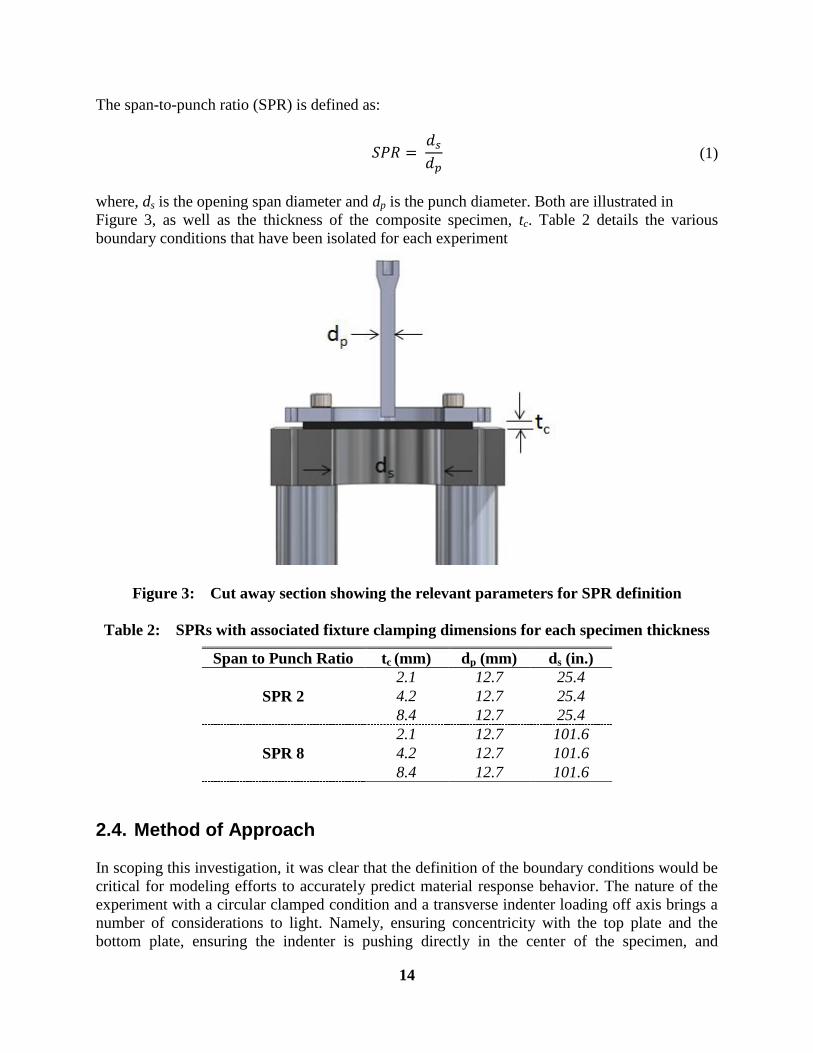
The span-to-punch ratio (SPR) is defined as:
𝑆𝑃𝑅 = 𝑑𝑠
𝑑𝑝 (1)
where, ds is the opening span diameter and dp is the punch diameter. Both are illustrated in
Figure 3, as well as the thickness of the composite specimen, tc. Table 2 details the various
boundary conditions that have been isolated for each experiment
Figure 3: Cut away section showing the relevant parameters for SPR definition
Table 2: SPRs with associated fixture clamping dimensions for each specimen thickness
Span to Punch Ratio tc (mm) dp (mm) ds (in.)
SPR 2
2.1 12.7 25.4
4.2 12.7 25.4
8.4 12.7 25.4
SPR 8
2.1 12.7 101.6
4.2 12.7 101.6
8.4 12.7 101.6
2.4. Method of Approach
In scoping this investigation, it was clear that the definition of the boundary conditions would be
critical for modeling efforts to accurately predict material response behavior. The nature of the
experiment with a circular clamped condition and a transverse indenter loading off axis brings a
number of considerations to light. Namely, ensuring concentricity with the top plate and the
bottom plate, ensuring the indenter is pushing directly in the center of the specimen, and

15
ensuring there is a well characterized and repeatable clamping force when the fixture is engaged
on the specimen.
The clamping fixture consists of a top plate which is securely fastened to the bottom plate with
threaded holes and bolts. The specimen is placed beneath the top plate and held securely in place
when the top plate is bolted down to the bottom plate. The specimens, as previously noted, have
bolt holes cut into them to allow the clamping bolts to freely pass through. The specimen is then
clamped to a force defined by the bolt torque.
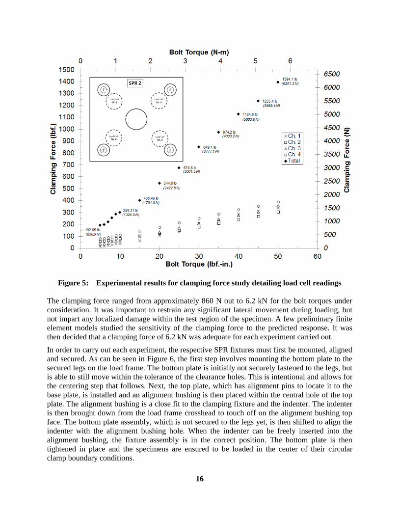
In order to determine the clamping force as a function of the bolt torque, a study was initially
carried out using button load cells and a torque wrench. The load cells were positioned in the
vicinity of the clamping bolts, directly under the top clamping plate. The bolts were oil
lubricated and then torqued to a range of values spanning from 0 up to to 5.65 Nm (50 lbf.-in.).
The details of the experimental set up and results can be seen in Figure 4 and Figure 5.
Load Cells in Place Top Plate Bolted down on Load Cells
Figure 4: Clamping force experimental set-up detailing button load cells and their
location
16
Figure 5: Experimental results for clamping force study detailing load cell readings
The clamping force ranged from approximately 860 N out to 6.2 kN for the bolt torques under
consideration. It was important to restrain any significant lateral movement during loading, but
not impart any localized damage within the test region of the specimen. A few preliminary finite
element models studied the sensitivity of the clamping force to the predicted response. It was
then decided that a clamping force of 6.2 kN was adequate for each experiment carried out.
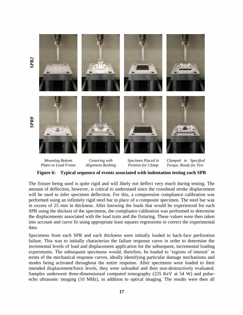
In order to carry out each experiment, the respective SPR fixtures must first be mounted, aligned
and secured. As can be seen in Figure 6, the first step involves mounting the bottom plate to the
secured legs on the load frame. The bottom plate is initially not securely fastened to the legs, but
is able to still move within the tolerance of the clearance holes. This is intentional and allows for
the centering step that follows. Next, the top plate, which has alignment pins to locate it to the
base plate, is installed and an alignment bushing is then placed within the central hole of the top
plate. The alignment bushing is a close fit to the clamping fixture and the indenter. The indenter
is then brought down from the load frame crosshead to touch off on the alignment bushing top
face. The bottom plate assembly, which is not secured to the legs yet, is then shifted to align the
indenter with the alignment bushing hole. When the indenter can be freely inserted into the
alignment bushing, the fixture assembly is in the correct position. The bottom plate is then
tightened in place and the specimens are ensured to be loaded in the center of their circular
clamp boundary conditions.
17
S
PR
2
SP
R8
Mounting Bottom
Plates to Load Frame
Centering with
Alignment Bushing
Specimen Placed in
Position for Clamp
Clamped to Specified
Torque, Ready for Test
Figure 6: Typical sequence of events associated with indentation testing each SPR
The fixture being used is quite rigid and will likely not deflect very much during testing. The
amount of deflection, however, is critical to understand since the crosshead stroke displacement
will be used to infer specimen deflection. For this, a compression compliance calibration was
performed using an infinitely rigid steel bar in place of a composite specimen. The steel bar was
in excess of 25 mm in thickness. After knowing the loads that would be experienced for each
SPR using the thickest of the specimens, the compliance calibration was performed to determine
the displacements associated with the load train and the fixturing. These values were then taken
into account and curve fit using appropriate least squares regressions to correct the experimental
data.
Specimens from each SPR and each thickness were initially loaded to back-face perforation
failure. This was to initially characterize the failure response curve in order to determine the
incremental levels of load and displacement application for the subsequent, incremental loading
experiments. The subsequent specimens would, therefore, be loaded to ‘regions of interest’ in
terms of the mechanical response curves, ideally identifying particular damage mechanisms and
modes being activated throughout the entire response. After specimens were loaded to their
intended displacement/force levels, they were unloaded and then non-destructively evaluated.
Samples underwent three-dimensionsal computed tomography (225 KeV at 54 W) and pulse-
echo ultrasonic imaging (10 MHz), in addition to optical imaging. The results were then all

18
compiled and used to define the failure process involved for each SPR and thickness. These
experiments serve as the validation experiments for the finite element predictions.
All testing was carried out on an Instron 5989 universal load frame, controlled using BlueHill
software. All loading and unloading were controlled using crosshead stroke displacement at 3
mm/min, and data was collected at 10 Hz.
2.5. Experimental Results
The load versus displacement curves have been developed for each SPR for each of the 3
thicknesses. The optical, ultrasonic and computed tomography (CT) imaging is shown for each
series of experimental results and will aid in the discussion. The results are broken up into SPR2
and SPR8, with each stack sequence considered listed in order of lowest to highest thickness.
2.5.1. SPR 2 – 6 Ply
The response of the SPR 2 specimens all followed a similar trend to one another. An initial linear
ramp up to a critical force value preceded a load drop, which then stabilized and then began
increasing in load following the redistribution.
The response of the 6-ply laminates can be seen in Figure 7. The initial critical load for these
laminates is approximately 3.7 kN with an initial linear ramp having a slope of 12.6 kN/mm. The
maximum load achieved was approximately 9.1 kN. After identifying the failure behavior of 2
specimens, incrementally loaded specimens were then loaded (and unloaded) out to 0.285 mm,
0.93 mm and 2.0 mm of transverse displacement. These values were of interest for modelers to
understand what damage events were taking place up to these loading displacement levels. The
response curves for each of the incrementally loaded specimens are superposed over the failure
response curves in Figure 7.

19
Figure 7: Load-displacement response for SPR2 – 6 Ply
Images and c-scans of the specimens tested at the incremental displacement levels can be seen in
Figure 8. The CT images can be seen in Figure 9 through Figure 11. The lowest displacement
level, which was still within the initial, linear region of the response curve, did not appear to
produce any noticeable damage from any of the NDE methods of inspection, and the unloading
curve was essentially co-linear with the loading curve with negligible energy absorbed in the
process. The subsequent load levels, however, did show signs of damage.
The specimens loaded out to 0.93 mm and 2.0 mm of transverse deflection clearly show a
surface indentation on their top faces where the steel indenter left an impression. The bottom
faces also show a blistering effect from the residual deflection. The ultrasonic images show clear
signal attenuation in the region just outside of the indenter, spanning approximately 2 times the
indenter diameter in both cases. Upon closer inspection of
Figure 10 and Figure 11, the true differences can be highlighted.
For the specimen loaded to 0.93 mm, there is a clear indentation and blistering but nothing
significant on the CT scan other than the permanent deformation induced. There is no evidence
of shear cracking from the CT images for this specimen. The specimen loaded out to 2.0 mm
shows a complex pattern of shear cracks in the matrix, originating from the local contact forces
of the indenter. There is localized evidence of inter-ply delamination emanating from the shear
cracks, beyond the indenter diameter, in both orthogonal directions, associated with the fiber
weave (up and down in c-scans), which appears to extend the c-scan signal attenuation beyond
its circular form. From the force-displacement response curve, it can be stated that the initial load
drop at approximately 0.33 mm is likely caused by small scale surface cracking around the

20
indenter, which leaves a permanent deformation. Beyond this point, shear cracking and small
scale delamination result as more energy is dissipated.
To
p F
ace
Bo
tto
m F
ace
C-S
can
δ = 0.285 mm δ = 0.93 mm δ = 2.0 mm
Figure 8: Images and c-scans of incrementally tested specimens for SPR2 – 6 Ply
Figure 9: Computed tomography slices of SPR2-6 ply at δ = 0.285 mm

21
Figure 10: Computed tomography slices of SPR2-6 ply at δ = 0.93 mm
Figure 11: Computed tomography slices of SPR2-6 ply at δ = 2.0 mm
2.5.2. SPR 2 – 12 Ply
The response of the 12-ply laminates can be seen in Figure 12. The initial critical load for these
laminates is approximately 8.3 kN with an initial linear ramp having a slope of 42 kN/mm. The
maximum load achieved was approximately 18.5 kN. After identifying the failure behavior of 2
specimens, incrementally loaded specimens were then loaded (and unloaded) out to 0.19 mm,
0.43 mm and 2.0 mm of transverse displacement.

22
Figure 12: Load-displacement response for SPR2 – 12 Ply
Images and c-scans of the specimens tested at the incremental displacement levels can be seen in
Figure 13. The CT images can be seen in Figure 14 through Figure 16. Similar to the previously
reported SPR2 – 6 ply, the lowest displacement level, which was still within the initial, linear
region of the response curve, did not appear to produce any noticeable damage from any of the
NDE methods of inspection, and the unloading curve was essentially co-linear with the loading
curve with negligible energy absorbed in the process. The subsequent load levels, however, did
show signs of damage.
The specimen loaded to 0.43 mm of transverse displacement shows a clear indentation from the
indenter as well as the blistering effect on the back face. This is the same for the specimen
loaded to a higher level of 2.0 mm. Both show similar c-scan signal attenuation, but the 2.0 mm
specimen, as previously noted for SPR2 – 6 ply, includes the localized delamination extending
from the shear cracks beyond the indenter region. These cracks and delaminations are evident in
the CT scans of Figure 16.

23
To
p F
ace
B
ott
om
Fa
ce
C-S
can
δ = 0.19 mm δ = 0.43 mm δ = 2.0 mm
Figure 13: Images and c-scans of incrementally tested specimens for SPR2 – 12 Ply
Figure 14: Computed tomography slices of SPR2-12 ply at δ = 0.19 mm

24
Figure 15: Computed tomography slices of SPR2-12 ply at δ = 0.43 mm
Figure 16: Computed tomography slices of SPR2-12 ply at δ = 2.0 mm
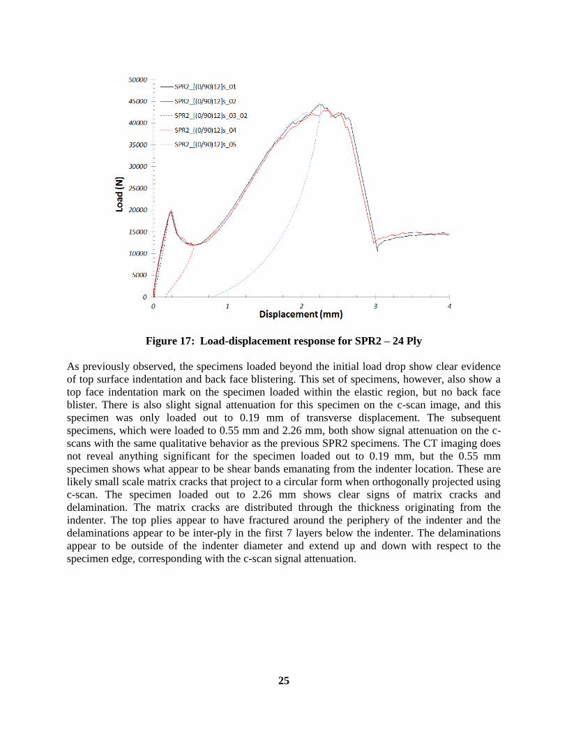
2.5.3. SPR 2 – 24 Ply
The response of the 24-ply laminates can be seen in Figure 17. The initial critical load for these
laminates is approximately 19.8 kN with an initial linear ramp having a slope of 82 kN/mm. The
maximum load achieved was approximately 43 kN. A noticeable feature on these response
curves is the significantly smooth response curve after the initial load drop as load is
redistributed and then increased. After identifying the failure behavior of 2 specimens,
incrementally loaded specimens were then loaded (and unloaded) out to 0.19 mm, 0.55 mm and
2.26 mm of transverse displacement.
25
Figure 17: Load-displacement response for SPR2 – 24 Ply
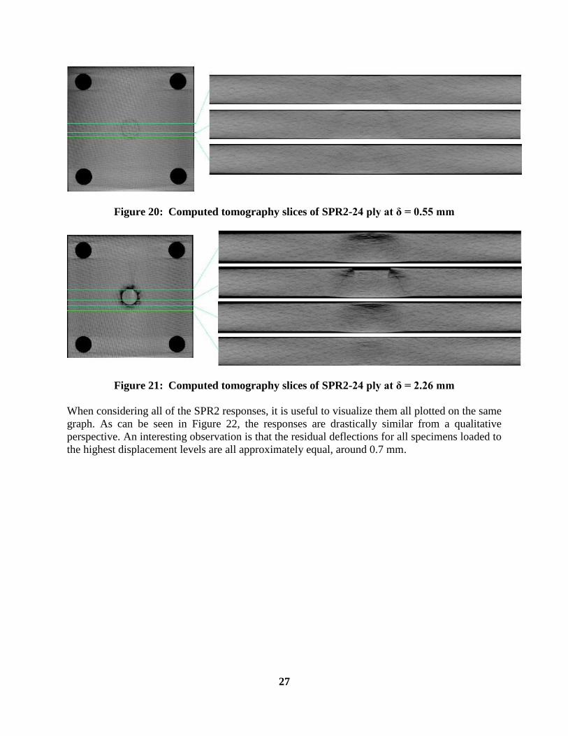
As previously observed, the specimens loaded beyond the initial load drop show clear evidence
of top surface indentation and back face blistering. This set of specimens, however, also show a
top face indentation mark on the specimen loaded within the elastic region, but no back face
blister. There is also slight signal attenuation for this specimen on the c-scan image, and this
specimen was only loaded out to 0.19 mm of transverse displacement. The subsequent
specimens, which were loaded to 0.55 mm and 2.26 mm, both show signal attenuation on the c-
scans with the same qualitative behavior as the previous SPR2 specimens. The CT imaging does
not reveal anything significant for the specimen loaded out to 0.19 mm, but the 0.55 mm
specimen shows what appear to be shear bands emanating from the indenter location. These are
likely small scale matrix cracks that project to a circular form when orthogonally projected using
c-scan. The specimen loaded out to 2.26 mm shows clear signs of matrix cracks and
delamination. The matrix cracks are distributed through the thickness originating from the
indenter. The top plies appear to have fractured around the periphery of the indenter and the
delaminations appear to be inter-ply in the first 7 layers below the indenter. The delaminations
appear to be outside of the indenter diameter and extend up and down with respect to the
specimen edge, corresponding with the c-scan signal attenuation.

26
To
p F
ace
B
ott
om
Fa
ce
C-S
can
δ = 0.19 mm δ = 0.55 mm δ = 2.26 mm
Figure 18: Images and c-scans of incrementally tested specimens for SPR2 – 24 Ply
Figure 19: Computed tomography slices of SPR2-24 ply at δ = 0.19 mm
27
Figure 20: Computed tomography slices of SPR2-24 ply at δ = 0.55 mm
Figure 21: Computed tomography slices of SPR2-24 ply at δ = 2.26 mm
When considering all of the SPR2 responses, it is useful to visualize them all plotted on the same
graph. As can be seen in Figure 22, the responses are drastically similar from a qualitative
perspective. An interesting observation is that the residual deflections for all specimens loaded to
the highest displacement levels are all approximately equal, around 0.7 mm.

28
Figure 22: All SPR2 results – 6 ply, 12 ply and 24 ply -- plotted together
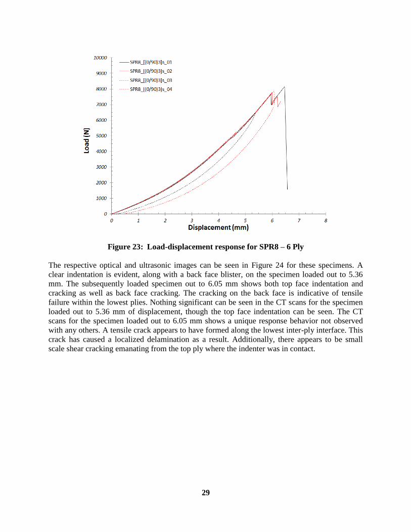
2.5.4. SPR 8 – 6 Ply
Unlike the SPR2 specimens, the SPR8 specimens exhibit a significantly noticeable difference in
response behavior characteristics. This is most noticeable for the SPR8 6-ply laminates when
comparing with the 12 or 24 ply laminates. As can be seen in Figure 23, the SPR8 6 ply
laminates exhibit a non-linear response out to an initial load drop at approximately 7.7 kN. Two
regions of interest were defined for this series of specimens, one just below the initial load drop
and one just after it. The displacement levels tested to for these specimens were 5.36 mm and
6.05 mm.
29
Figure 23: Load-displacement response for SPR8 – 6 Ply
The respective optical and ultrasonic images can be seen in Figure 24 for these specimens. A
clear indentation is evident, along with a back face blister, on the specimen loaded out to 5.36
mm. The subsequently loaded specimen out to 6.05 mm shows both top face indentation and
cracking as well as back face cracking. The cracking on the back face is indicative of tensile
failure within the lowest plies. Nothing significant can be seen in the CT scans for the specimen
loaded out to 5.36 mm of displacement, though the top face indentation can be seen. The CT
scans for the specimen loaded out to 6.05 mm shows a unique response behavior not observed
with any others. A tensile crack appears to have formed along the lowest inter-ply interface. This
crack has caused a localized delamination as a result. Additionally, there appears to be small
scale shear cracking emanating from the top ply where the indenter was in contact.

30
To
p F
ace
Bo
tto
m F
ace
C-S
can
δ = 5.36 mm δ = 6.05 mm
Figure 24: Images and c-scans of incrementally tested specimens for SPR8 – 6 Ply
Figure 25: Computed tomography slices of SPR8-6 ply at δ = 5.36 mm

31
Figure 26: Computed tomography slices of SPR8-6 ply at δ = 6.05 mm
2.5.5. SPR 8 – 12 Ply
The response of the 12-ply laminates can be seen in Figure 27. The initial critical load for these
laminates is approximately 7.7 kN with an initial linear ramp having a slope of 4.3 kN/mm. The
maximum load achieved was approximately 19 kN. After identifying the failure behavior of 2
specimens, incrementally loaded specimens were then loaded (and unloaded) out to 1.61 mm,
2.85 mm and 4.8 mm of transverse displacement.
Figure 27: Load-displacement response for SPR8 – 12 Ply
Unlike previous specimens, there are no indications on any of the back faces of cracking or
blister formation which can be seen in
32
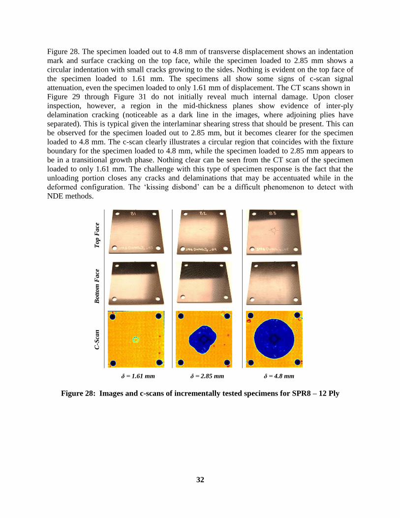
Figure 28. The specimen loaded out to 4.8 mm of transverse displacement shows an indentation
mark and surface cracking on the top face, while the specimen loaded to 2.85 mm shows a
circular indentation with small cracks growing to the sides. Nothing is evident on the top face of
the specimen loaded to 1.61 mm. The specimens all show some signs of c-scan signal
attenuation, even the specimen loaded to only 1.61 mm of displacement. The CT scans shown in
Figure 29 through Figure 31 do not initially reveal much internal damage. Upon closer
inspection, however, a region in the mid-thickness planes show evidence of inter-ply
delamination cracking (noticeable as a dark line in the images, where adjoining plies have
separated). This is typical given the interlaminar shearing stress that should be present. This can
be observed for the specimen loaded out to 2.85 mm, but it becomes clearer for the specimen
loaded to 4.8 mm. The c-scan clearly illustrates a circular region that coincides with the fixture
boundary for the specimen loaded to 4.8 mm, while the specimen loaded to 2.85 mm appears to
be in a transitional growth phase. Nothing clear can be seen from the CT scan of the specimen
loaded to only 1.61 mm. The challenge with this type of specimen response is the fact that the
unloading portion closes any cracks and delaminations that may be accentuated while in the
deformed configuration. The ‘kissing disbond’ can be a difficult phenomenon to detect with
NDE methods.
To
p F
ace
Bo
tto
m F
ace
C-S
can
δ = 1.61 mm δ = 2.85 mm δ = 4.8 mm
Figure 28: Images and c-scans of incrementally tested specimens for SPR8 – 12 Ply

33
Figure 29: Computed tomography slices of SPR8-12 ply at δ = 1.61 mm
Figure 30: Computed tomography slices of SPR8-12 ply at δ = 2.85 mm
Figure 31: Computed tomography slices of SPR8-12 ply at δ = 4.8 mm
2.5.6. SPR 8 – 24 Ply
The response of the 24-ply laminates can be seen in Figure 32. The initial critical load for these
laminates is approximately 17.7 kN with an initial linear ramp having a slope of 20.3 kN/mm.
The maximum load achieved was approximately 36.7 kN. As with previous specimen groups,
after identifying the failure behavior of 2 specimens, incrementally loaded specimens were then
loaded (and unloaded) out to 0.75 mm, 1.12 mm and 2.72 mm, and 5.59 mm of transverse

34
displacement. There was an additional specimen loaded out to an intermediate displacement
level, but it did not provide significant or unique insight.
Figure 32: Load-displacement response for SPR8 – 24 Ply
Upon inspection of the specimens shown in Figure 33, signs of indentation loading are evident
on all top faces. There is a circular indentation which can be seen for the specimens loaded to
0.75 mm and 1.12 mm, along with the addition of transverse cracking for the specimens loaded
further to 2.72 mm and 5.59 mm. Ultrasonic signal attenuation is evident for all specimens in
this series, even the lowest loading level. The CT scans shown in Figure 34 and Figure 35 do not
reveal anything significant for the specimen loaded to 0.75 mm, and only a small, local shear
crack for the specimen loaded to 1.12 mm. Although the c-scan shows significantly clear signal
attenuation for the specimen loaded to 2.72 mm, the CT scans of Figure 36 for this specimen are
not as clear. Upon closer inspection for this specimen, however, a delamination can be seen just
below the mid-thickness plane, and another approximately ¼ of the way up from the bottom. The
specimen loaded out to 5.59 mm shows a highly complex network of inter-ply delamination and
upper ply cracking in the CT scans of Figure 37. The delaminations do not appear to be below
the indenter, but only outward from it. The delaminations appear to be uniformly distributed
throughout the thickness.

35
To
p F
ace
Bo
tto
m F
ace
C-S
can
δ = 0.75 mm δ = 1.12 mm δ = 2.72 mm δ = 5.59 mm
Figure 33: Images and c-scans of incrementally tested specimens for SPR8 – 24 Ply
Figure 34: Computed tomography slices of SPR8-24 ply at δ = 0.75 mm
Figure 35: Computed tomography slices of SPR8-24 ply at δ = 1.12 mm
36
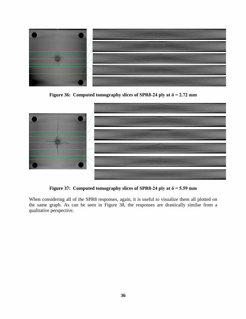
Figure 36: Computed tomography slices of SPR8-24 ply at δ = 2.72 mm
Figure 37: Computed tomography slices of SPR8-24 ply at δ = 5.59 mm
When considering all of the SPR8 responses, again, it is useful to visualize them all plotted on
the same graph. As can be seen in Figure 38, the responses are drastically similar from a
qualitative perspective.

37
Figure 38: All SPR8 results – 6 ply, 12 ply and 24 ply -- plotted together
2.6. Conclusions
From the experimental portion of this investigation, the following conclusions can be made for
the specimen configurations considered:
1. All SPR2 responses in this study are initially linear in their load-deflection response.
2. All SPR2 specimens loaded beyond the initial load drop show a clear indication of
indentation damage on both the top and bottom faces of the specimen when optically
viewed.
3. All SPR2 specimens experience shear cracking first, followed by delamination. The
delamination locations are governed by the extent of shear cracking and appear to be
caused as a result.
4. SPR8 specimens show inter-ply delamination without the precipitation from matrix shear
cracking. It appears to be initiated from interlaminar shearing stress.
5. No bottom face damage was evident for most SPR8 specimens, unless they are thin
enough to experience excessive tensile stresses from flexure.
6. Shear matrix cracking and inter-ply delamination cracking show similar signal
attenuation to one another with ultrasonic c-scans.

38

39
3. FINITE ELEMENT MODEL
With the experimental results available, the investigation now moves into the modeling and
simulation realm to gain additional insight into the time sequence of events that may govern the
response and to validate the damage mechanisms and modes governing material failure.
In general, finite element analysis is used in the following facets:
Verification and elucidation of failure mode assumptions in the model
Exploration of alternative modeling methods
Validation of various failure modes
Exposing model deficiencies and defining future work
This section will describe the mesh details, underlying assumptions, simplifications, sensitivities
and verification efforts.
3.1. Mesh
Reduced integration hexahedral elements with a default hourglass stiffness of 0.05 are used in
the lamina and fixture. Each lamina interface is modeled as a plane separated by cohesive zone
(CZ) or localization zero volume hexahedral elements in order to capture delamination failure.
For example, for a 12 layer laminate with one element through the thickness or each lamina there
are 23 elements through the thickness, 12 solid hexahedral and 11 CZ surface elements.
Three types of meshes are used in this analysis. All the meshes are model with quarter
symmetry. The first mesh type, shown in Figure 39, is a high fidelity geometric representation
of the top and bottom clamping plates, a simplified bolt and the specimen. This mesh has a 1:1
aspect ratio near the indenter, with one element per lamina. This level of mesh refinement is not
expected to be sufficient to capture local failure in the composite induced by the relatively sharp
indenter. However, this level of refinement has been shown to accurately capture distributed
damage and delamination under impact conditions [2]. The second mesh, shown in Figure 40,
has a substantially reduced fixture and is topologically similar near the indenter. The third mesh
type is has a similar geometry to the previous with an estimate for the fillet in the indenter and a
local refinement region near the indenter. A local refinement with four elements through the
thickness of each lamina is shown in Figure 41.

40
Figure 39: Coarse mesh for the SPR = 2, full geometry
Figure 40: Coarse mesh for the SPR = 2, reduced geometry

41
Figure 41: Mesh refinement and punch fillet applied to refined models
3.2. Geometric Sensitivity
Due to the high loads experienced in this experiment the load versus displacement results are
extremely sensitive to fixture compliance. While the data is corrected for fixture compliance
some error is expected. Effort is given to verify local stresses and strains for a given applied
load are minimally affected by fixturing. This study is also used to justify the use of a simplified
model geometry. Three considerations are made in the geometric representation of the
experiment in order to simplify the model. First, the preload on the bolts is investigated.
Second, the extent of the fixture is reduced and the effects are quantified. Third, fixed top
clamping plate conditions are considered.
Errors from geometric assumptions are estimated by comparing load versus displacement of
aluminum samples. Aluminum, which is adequately modeled as elastic isotropic, is used in
order to reduce uncertainty in the material model. Panels with a thickness of 3.175 mm are
tested in the same configuration as the composite laminates for both SPR = 2 and 8.
Figure 42 shows the compliance comparison of a geometrically accurate top and bottom plate,
bolts and preload. The preload is applied by an artificial strain in the bolt that is calibrated to
give the 6201 N preload described in the experimental method section. The differences in the
model and experiment are a combination of experimental errors, such as compliance correction
and measurement errors, and numerical errors, such as discretization and material uncertainty. A
full uncertainty quantification analysis would be required to provide a statically relevant offset.
This is not completed in this study and this data serves only as a qualitative assessment on the
accuracy of the load versus displacement model experiment comparisons.

42
Figure 42: Aluminum panel model compliance validation
Figure 43 shows the SPR = 2 and 8 simulations with and without preload. The high fidelity
meshes for the aluminum experiments are used. The artificial strain method is used to impart the
correct preload. In the case of no preload, zero strain is applied. It is clear that the effects of
preload are minimal. Increased slippage in the SPR = 8 results in more noticeable stiffness loss;
however the risk of neglecting the preload is deemed acceptable.

43
Figure 43: Aluminum panel model compliance preload sensitivity
Figure 44 shows the load versus displacement response comparison between the high fidelity and
simplified models with preloads. These models are described in Section 3.1. As might be
expected, the high aspect ratio response (SPR = 8) is more influenced by slippage in the clamps.
The simplified model is more constrained due to the fixed top assumption and therefore appears
stiffer. Since the difference in the SPR = 8 full versus simplified models is more pronounced a
local metric is investigated to justify simplification. The max out-of-plane shear stress at the
neutral axis is used to compare the local differences in the full versus simplified models. For
SPR = 2, the full and simplified stresses interpolated at 4000 N applied load are 39.4 MPa and
39.2 MPa, respectively. The simplified geometry produces a negligible -0.51% error. For SPR
= 8, the full and simplified stresses interpolated at 1000 N applied load are 9.42 MPa and 9.49
MPa, respectively. The simplified geometry produces a slightly higher 0.74% error. The results
of this sensitivity study indicate the errors to be small when using a simplified geometry for
model size reduction. Moreover, thin geometries, such as the aluminum specimens, with larger
SPRs will show a greater dependence on the clamping boundary conditions. For this study, the
majority of the work will be completed with these simplified geometries without preload.

44
Figure 44: Aluminum panel fixture simplification sensitivity
3.3. Finite Element Code
The ranges of time periods present in the punch shear experiment necessitate the use of implicit
dynamic finite element method. More precisely, the duration of indentation is on the order of
10s of seconds and some failure processes are dynamic and happen over much shorter time
periods. The use of the implicit solver is prohibitively difficult. The difficulty of utilizing the
implicit solver is related to both contact and material failure. The combination of extensive
contact combined with material failure (delamination and fiber breaks) requires extremely small
timesteps when using adaptive time stepping. Moreover, it is uncertain if convergence is
possible under these conditions.
In order to verify the equivalence of the explicit dynamic simulations to the quasi-static reality, a
rate convergence study is completed. Rate dependencies in the material are ignored and no other
modifications to mass or damping are implemented. Three indentation rates are tested. These
rates are 125 mm/s, 250 mm/s and 500 mm/s. The coarse mesh SPR = 2, 12 layer geometry is
chosen. The load versus displacement results are shown in Figure 45. It is clear that the slower
rates, 125 and 250 mm/s, are nearly identical indicating near quasi-static conditions. All
simulations are conducted with a maximum of 250 mm/s. Most simulations are conducted at 125
mm/s.

45
Figure 45: Indentation rate convergence
3.4. Materials
3.4.1. Elastic Orthotropic Failure
The formulation of the elastic orthotropic material model follows closely with [3-5]. Crack band
theory is implemented. Failure, or crack localization, is assumed to be distributed across the
crack band and softening is controlled by size-dependent fracture energy [6]. Since elastic
damage is assumed to be the only source of stiffness loss, damage variables can be introduced
for each of the normal and shear components of stress. The corresponding compliance tensor
takes on the following form [3]:
The damaged (actual) stresses and strains are
𝐒 =
[
1
𝐸11(1 − 𝑑11)
−𝜐21
𝐸22
−𝜐31
𝐸330 0 0
−𝜐12
𝐸11
1
𝐸22(1 − 𝑑22)
−𝜐32
𝐸330 0 0
−𝜐13
𝐸11
−𝜐23
𝐸22
1
𝐸33(1 − 𝑑33)0 0 0
0 0 01
2𝐺12(1 − 𝑑12)0 0
0 0 0 01
2𝐺13(1 − 𝑑13)0
0 0 0 0 01
2𝐺23(1 − 𝑑23)]
(2)

46
𝜎𝑖𝑗 = 𝐶𝑖𝑗𝑘𝑙휀𝑘𝑙 (3)
휀𝑖𝑗 = 𝑆𝑖𝑗𝑘𝑙𝜎𝑘𝑙 (4)
where
𝐶𝑖𝑗𝑘𝑙 = 𝑆𝑖𝑗𝑘𝑙−1 (5)
Since the compliance tensor becomes singular at d = 1, the stiffness tensor is written in closed
form where the limit of stiffness as d → 1 exists.
A quadratic strain criterion is used for damage initiation and failure. The damage activation
threshold is evaluated for tension and compression, matrix and fiber modes and for each of the
primary material planes [4, 5, 7]. The damage activation function for the matrix mode in the 11
plane is given for tension and compression as
Tension: 𝜑11+𝑚 = √(
𝐸11⟨휀11⟩
𝑋11+𝑚 )
2
+ (𝐺12𝛾12
𝑆12𝑚 )
2
+ (𝐺13𝛾13
𝑆13𝑚 )
2
(6)
Compression: 𝜑11−𝑚 = √(
𝐸11⟨−휀11⟩
𝑋11−𝑚 )
2
+ (𝐺12𝛾12
𝑆12𝑚 )
2
+ (𝐺13𝛾13
𝑆13𝑚 )
2
(7)
where ⟨ ⟩ are the Macaulay brackets, defined as
⟨𝑥⟩ = {0, 𝑥 < 0𝑥, 𝑥 ≥ 0
(8)
The user provides only damage initiation/failure stresses (𝑋𝑓). For failure in the fiber mode the
stress used in the damage activation function must be the effective stress. For strain equivalency,
the effective strength in the 11 direction is simply
�̅�𝑓
= 𝐸11휀11𝑓
(9)
where 휀11𝑓
is the strain to fiber failure. Therefore, the damage activation function for the fiber
mode in the 11 plane is given for tension and compression as
Tension: 𝜑11+𝑓
= √(𝐸11⟨휀11⟩
�̅�11+𝑓
)
2
+ (𝐺12𝛾12
𝑆̅12𝑓
)
2
+ (𝐺13𝛾13
𝑆̅13𝑓
)
2
(10)
Compression: 𝜑11−𝑓
= √(𝐸11⟨−휀11⟩
�̅�11−𝑓
)
2
+ (𝐺12𝛾12
𝑆̅12𝑓
)
2
+ (𝐺13𝛾13
𝑆̅13𝑓
)
2
(11)

47
A special criterion is given for out-of-plane compressive failure. This crush type is simply
modeled using a maximum strain criterion with no shear coupling. The damage activation
function is
Out-of-plane
Compression: 𝜑33−
𝑓=
𝐸33⟨−휀11⟩
�̅�33−𝑓
(12)
The user specified fracture energy for a given mode of failure is the total energy associated with
material bifurcation in this mode. The current model formulation does not account for mixed
mode coupling during fracture.
Crack band theory assumes that a band of continuously distributed parallel cracks [6] produces
the same energy released as line crack. The opening stress to relative displacement (δ)
relationship is therefore replaced with the presumed identical δ = εl*, where, l
* is the
characteristic length of the finite element and ε is the homogenized strain in the crack opening
direction [5].
Damage evolution is user defined only for matrix mode failure. The evolution of fiber damage is
controlled by internal parameters using the fracture energies and crack band theory. For each
matrix failure mode (tension, compression, shear), the evolution equation is generally defined as
𝑑 = 1 −𝐾𝑚
𝐸+ (
𝐾𝑚
𝐸− 1)
1
𝑟𝑚𝑛 (13)
where Km and n are the matrix mode damage modulus and exponent respectively. The damage
exponent is intended to add flexibility in the material response. For shear damage, Km is defined
in τ - γ space. After the fiber mode strength is exceeded, the material is linearly softened. Note
matrix mode damage is zero for Km = E or n = 0.
The properties for the 8HS CFRP are shown in Table 3. Standard deviations are given in
parentheses and bounds of uniform distributions are shown as ±. Very large ranges are often
utilized in the sensitivity analysis due to lack of decent predictions. Once deemed influential, the
parameters are better estimated.
48
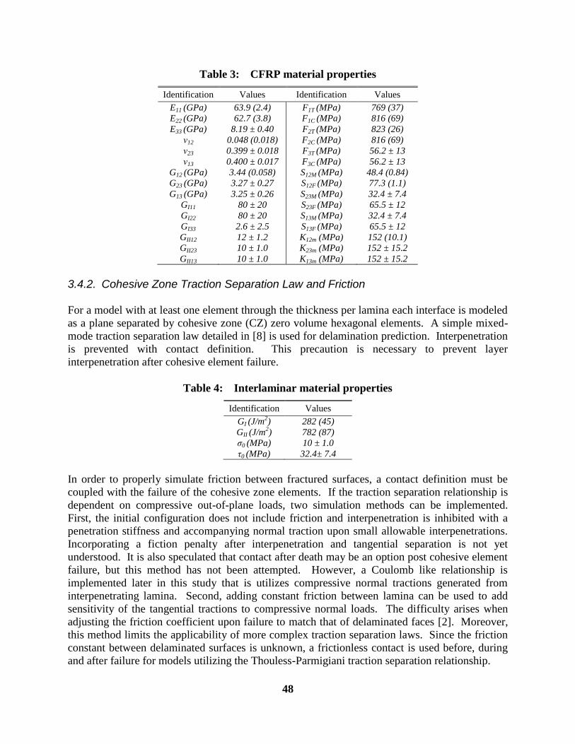
Table 3: CFRP material properties
Identification Values Identification Values
E11 (GPa)
E22 (GPa)
E33 (GPa)
ν12
ν23
ν13
G12 (GPa)
G23 (GPa)
G13 (GPa)
GI11
GI22
GI33
GII12
GII23
GII13
63.9 (2.4)
62.7 (3.8)
8.19 ± 0.40
0.048 (0.018)
0.399 ± 0.018
0.400 ± 0.017
3.44 (0.058)
3.27 ± 0.27
3.25 ± 0.26
80 ± 20
80 ± 20
2.6 ± 2.5
12 ± 1.2
10 ± 1.0
10 ± 1.0
F1T (MPa)
F1C (MPa)
F2T (MPa)
F2C (MPa)
F3T (MPa)
F3C (MPa)
S12M (MPa)
S12F (MPa)
S23M (MPa)
S23F (MPa)
S13M (MPa)
S13F (MPa)
K12m (MPa)
K23m (MPa)
K13m (MPa)
769 (37)
816 (69)
823 (26)
816 (69)
56.2 ± 13
56.2 ± 13
48.4 (0.84)
77.3 (1.1)
32.4 ± 7.4
65.5 ± 12
32.4 ± 7.4
65.5 ± 12
152 (10.1)
152 ± 15.2
152 ± 15.2
3.4.2. Cohesive Zone Traction Separation Law and Friction
For a model with at least one element through the thickness per lamina each interface is modeled
as a plane separated by cohesive zone (CZ) zero volume hexagonal elements. A simple mixed-
mode traction separation law detailed in [8] is used for delamination prediction. Interpenetration
is prevented with contact definition. This precaution is necessary to prevent layer
interpenetration after cohesive element failure.
Table 4: Interlaminar material properties
Identification Values
GI (J/m2)
GII (J/m2)
σ0 (MPa)
τ0 (MPa)
282 (45)
782 (87)
10 ± 1.0
32.4± 7.4
In order to properly simulate friction between fractured surfaces, a contact definition must be
coupled with the failure of the cohesive zone elements. If the traction separation relationship is
dependent on compressive out-of-plane loads, two simulation methods can be implemented.
First, the initial configuration does not include friction and interpenetration is inhibited with a
penetration stiffness and accompanying normal traction upon small allowable interpenetrations.
Incorporating a fiction penalty after interpenetration and tangential separation is not yet
understood. It is also speculated that contact after death may be an option post cohesive element
failure, but this method has not been attempted. However, a Coulomb like relationship is
implemented later in this study that is utilizes compressive normal tractions generated from
interpenetrating lamina. Second, adding constant friction between lamina can be used to add
sensitivity of the tangential tractions to compressive normal loads. The difficulty arises when
adjusting the friction coefficient upon failure to match that of delaminated faces [2]. Moreover,
this method limits the applicability of more complex traction separation laws. Since the friction
constant between delaminated surfaces is unknown, a frictionless contact is used before, during
and after failure for models utilizing the Thouless-Parmigiani traction separation relationship.
49
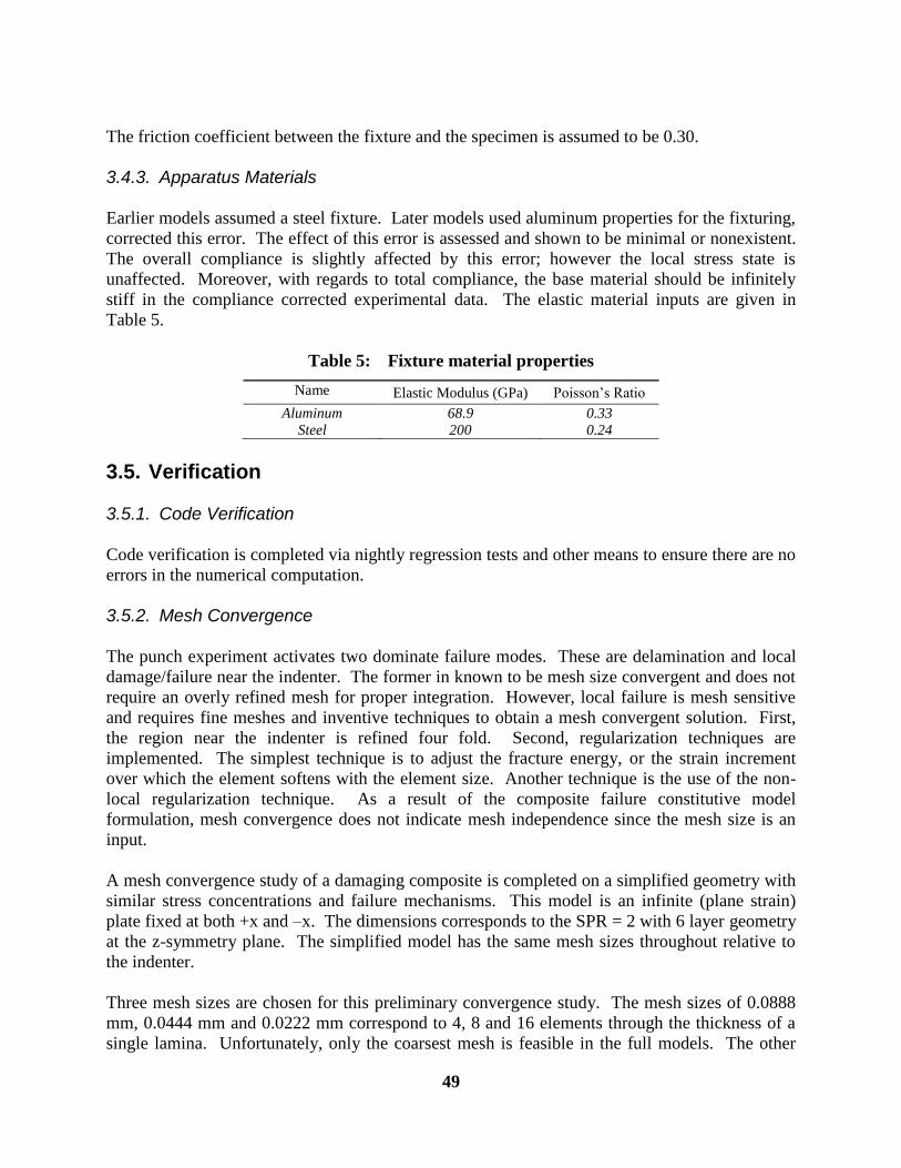
The friction coefficient between the fixture and the specimen is assumed to be 0.30.
3.4.3. Apparatus Materials
Earlier models assumed a steel fixture. Later models used aluminum properties for the fixturing,
corrected this error. The effect of this error is assessed and shown to be minimal or nonexistent.
The overall compliance is slightly affected by this error; however the local stress state is
unaffected. Moreover, with regards to total compliance, the base material should be infinitely
stiff in the compliance corrected experimental data. The elastic material inputs are given in
Table 5.
Table 5: Fixture material properties
Name Elastic Modulus (GPa) Poisson’s Ratio
Aluminum
Steel
68.9
200
0.33
0.24
3.5. Verification
3.5.1. Code Verification
Code verification is completed via nightly regression tests and other means to ensure there are no
errors in the numerical computation.
3.5.2. Mesh Convergence
The punch experiment activates two dominate failure modes. These are delamination and local
damage/failure near the indenter. The former in known to be mesh size convergent and does not
require an overly refined mesh for proper integration. However, local failure is mesh sensitive
and requires fine meshes and inventive techniques to obtain a mesh convergent solution. First,
the region near the indenter is refined four fold. Second, regularization techniques are
implemented. The simplest technique is to adjust the fracture energy, or the strain increment
over which the element softens with the element size. Another technique is the use of the non-
local regularization technique. As a result of the composite failure constitutive model
formulation, mesh convergence does not indicate mesh independence since the mesh size is an
input.
A mesh convergence study of a damaging composite is completed on a simplified geometry with
similar stress concentrations and failure mechanisms. This model is an infinite (plane strain)
plate fixed at both +x and –x. The dimensions corresponds to the SPR = 2 with 6 layer geometry
at the z-symmetry plane. The simplified model has the same mesh sizes throughout relative to
the indenter.
Three mesh sizes are chosen for this preliminary convergence study. The mesh sizes of 0.0888
mm, 0.0444 mm and 0.0222 mm correspond to 4, 8 and 16 elements through the thickness of a
single lamina. Unfortunately, only the coarsest mesh is feasible in the full models. The other

50
more refined meshes would be far too expensive to run. Figure 46 shows the load displacement
results for these simulations. The first peak, corresponding to the propagation of the first
delamination, is similar between all three meshes and is convergent with mesh size. Figure 47
provides the relative discretization error (RDE) for this metric. The second point of significant
delamination is more influenced by local damage and therefore the coarsest mesh is an outlier
due to different delamination patterns. Figure 48 shows the meshes and damage patterns for
each of the meshes used.
Figure 46: Load versus displacement for the simplified mesh study geometries

51
Figure 47: Percent elative discretization error on the load at first delamination

52
a)
b)
c)
Figure 48: Coarse (a), medium (b) and fine (c) meshes with out-of-plane shear damage at
0.8mm of applied displacement

53
A second mesh convergence study is conducted in a companion paper [9]. This study utilizes
elastic properties and localization elements between lamina. This study shows good mesh
convergence for metrics far from the indenter, such as the maximum interlaminar sheer stress.
3.6. Sensitivity Analysis
A complete sensitivity analysis is conducted on the coarse mesh SPR = 2, 12 layer model. Three
metrics are calculated: the elastic slope, the first peak (proportional limit) and the secondary
slope after reload. Given the approximate symmetry of the geometry and the material, some
parameters are changed simultaneously to the same values in the sampling routine in order to
reduce the total number of variable tested. For example, the warp and weft elastic moduli are
nearly equal and variation in their values will have the same effect on the response, therefore E11
= E22 for the sensitivity analysis. The full list of parameters is given in Table 6 along with the
normalized results. Utilizing the Box Behnken Design of experiments method the total number
of runs with 22 inputs is 925.
A simple yet insightful metric to measure influence is the normalized general linear regression
weights. A multi-way analysis of variances method is used to perform a general linear
regression on the sensitivity model results. Each input is normalized to vary between -1 and 1.
The general linear regression weights are shown for each input in Table 6.

54
Table 6: SPR = 2, 12 layer general linear regression weights
Source Elastic Slope First Peak Damaged Slope
E11 393.79 35.98 -22.01
E33 402.74 -1.96 44.25
G12 66.20 6.72 -118.88
G23 2253.10 2.03 -18.68
TENSILE_FIBER_STRENGTH_11 0.00 0.00 -15.12
COMPRESSIVE_FIBER_STRENGTH_11 0.01 -0.14 0.05
TENSILE_FIBER_STRENGTH_33 0.00 0.00 0.33
COMPRESSIVE_FIBER_STRENGTH_33 114.45 -27.23 -87.36
SHEAR_MATRIX_STRENGTH_12 0.00 -0.03 623.75
SHEAR_FIBER_STRENGTH_12 0.00 0.00 -3.83
SHEAR_FIBER_STRENGTH_23 -55.50 10.01 37.40
TENSILE_FRACTURE_ENERGY_11 0.00 0.00 12.96
COMPRESSIVE_FRACTURE_ENERGY_11 -0.01 -0.05 15.74
COMPRESSIVE_FRACTURE_ENERGY_33 0.74 0.44 -3.45
SHEAR_FRACTURE_ENERGY_12 0.00 0.00 10.69
SHEAR_FRACTURE_ENERGY_23 0.85 1.23 10.52
SHEAR_DAMAGE_MODULUS_12 0.00 0.01 75.48
CZ_ENERGY_I 0.00 0.00 -6.49
CZ_ENERGY_II 2.34 50.75 -176.22
CZ_PEAK_TRAC_I 0.00 0.00 15.92
CZ_PEAK_TRAC_II -9.59 460.09 109.88
FRICTION_COEF 54.00 20.08 -7.90
The results of the sensitivity analysis are as expected. The first metric, denoted elastic slope, is
heavily dependent on the elastic moduli; the most influential being the out-of-plane shear
moduli. Post delamination, there is a transition from out-of-plane shear to in-plane tension. This
is elucidated by the model’s sensitivity to the out-of-plane shear modulus under elastic loading
and the in-plane shear matrix strength after delamination. The initiation of delamination, which
determines the proportional limit, is controlled by the interlaminar shear strength.

55
4. FINITE ELEMENT RESULTS
4.1. Locally refined model
In order to accurately capture the failure predicted by the model, a refined mesh is simulated for
the SPR = 2, 12 layer, SPR = 8, 12 layer and SPR = 8, 6 layer geometries. The mesh described
in Section 3.1 has a locally refined region that can capture the distributed shear and crush
damage as well as the localized shear failure. This model is used to distinguish between the
effects of lamina damage and delamination on the load versus displacement. Unfortunately,
simulations often timed out or failed due to a numerical issue before reaching the applied
displacement reflected in the experiments. This section will discuss results from the data
acquired.
Overall the results from the refined mesh simulations are not surprising. The known deficiencies
in the simulation, such as friction on delaminated faces, mesh dependencies and compression
sensitive delamination initiation, are demonstrated in these results. Nevertheless, the qualitative
results are inspiring and prove the models are on the correct path. Investigation into the other
geometries not mentioned in this section would be beneficial. However, prioritizing based on
time constraints and similarities in results was necessary.
4.1.1. SPR = 2, 12 layer
Figure 49 shows a portion of the load displacement results for both the refined model and an
experiment of the SPR = 2, 12 layer geometry. Figure 50 shows damage contours at the z-
symmetry plane at significant damaging events.
The load versus displacement results show the combination of distributed damage and smooth
deamination propagation at the mid-plane result in a gradual load loss not seen in the
experiments. Then after full delamination at the mid-plane the results show further delamination
at interfaces outside the mid-plane resulting in sudden load losses more indicative of the
experiments. However, the extent and distribution of delamination at the end of the simulation
do not match experiments. This is evident in the investigation of the CT and US scans as well as
discrepancies in the post delamination slope (damaged slope) in the numerical data. The
remaining stiffness after initial damage (displacement greater than 0.60) is most often less in the
simulation compared to experiments. Similar results are presented in the subsequent section
using a coarse mesh for uncertainty quantification.

56
Figure 49: SPR = 2, 12 layer preliminary load versus displacement

57
Displacement = 0.023 mm
Local out-of-plane shear and crush
damage.
No delamination
Displacement = 0.125 mm
Distributed out-of-plane shear and
crush damage.
Delamination near the mid-plane
between indenter and clamping fixture.
Displacement = 0.375 mm
Delaminations propagate to center and
begin to open in Mode I
Displacement = 0.50 mm
Additional delaminations propagate to
center and begin to open in Mode I
Figure 50: Damage evolution images and descriptions SPR = 2, 12 layers
4.1.2. SPR = 8, 12 layer
Figure 51 shows a portion of the load displacement results for both the refined model and an
experiment of the SPR = 8, 12 layer geometry. Figure 52 shows damage contours at the z-
symmetry plane at significant damaging events. The final image shows a localized shear crack
and a major delamination. Delamination is the major source of load loss in both the experiments
and simulation. In the model, the localized lamina failure precedes delamination resulting a
lower load and noisy data related to explicit analysis. This discrepancy is discussed in the
subsequent section.

58
Figure 51: SPR = 8, 12 layer preliminary load versus displacement

59
Displacement = 1.125 mm
Local out-of-plane shear and
crush damage
No delamination
Displacement = 1.35 mm
Localized shear failure in the top
half of lamina
Displacement = 1.875 mm
Full delamination between ply 4
and 5 (counting from the bottom)
Figure 52: Damage evolution images and descriptions SPR = 8, 12 layers
4.1.3. SPR = 8, 6 layer
Figure 53 shows the load displacement results for both the refined model and two experiments of
the SPR = 8, 12 layer geometry. Figure 54 shows damage contours at the z-symmetry plane at
significant damaging events. The SPR = 8, 6 layer geometry is a qualitative outlier. Unique to
this geometry, significant load loss is noticed in the absence of delamination. Local shear and
crush damage is the only active material non-linearity as is demonstrated in the early differences
between damaging and elastic solutions.
Due to the lack of descriptive experimental data, in-plane compression combined with out-of-
plane shear is not well described by the lamina material model. This may help describe the
premature failure localization in the numerical model. In reality, this type of failure may be
more distributed rather than localized. A similar phenomenon resulting in premature load loss is
seen in the previous section 4.1.2. SPR = 8, 12 layer. Nevertheless, by restricting compressive
damage, the force versus displacement results after localized failure match well to experiments.

60
However, it is unclear whether the model will be capable of predicting the violent rupture seen in
the experiments at penetration.
Figure 53: SPR = 8, 6 layer preliminary load versus displacement
Displacement = 2.25 mm
Local out-of-plane shear and
crush damage
No delamination
Displacement = 4.50 mm
Localized shear failure in the top
half of lamina
No significant delamination
Figure 54: Damage evolution images and descriptions SPR = 8, 6 layers

61
4.2. Quantitative Validation
It is clear from the elastic analysis conducted in the companion paper [9] and the refined damage
analysis presented above that in the majority of the geometries the first mode of failure resulting
in significant load loss is delamination. The proportional limit or first peak in the load
displacement curve does not exhibit significant discretization error with a coarse mesh.
Therefore, for a preliminary validation a coarse mesh is investigated
At the time of these simulations, a constitutive relationship that could accurately predict the
interlaminar strength increase under normal compressive loads did not exist. Therefore, the peak
tangential traction for the traction separation relationship is calibrated to match the mean
proportional limit in the experiments. It is expected that a constitutive relationship with the
aforementioned sensitivity will produce similar results. Nevertheless, this quantification of
uncertainty effort cannot be used to validate the model but does show significant progress and
conceptual confirmation.
Uncertainty quantification analysis of the SPR = 2, 12 layer geometry has been completed on the
proportional limit or the load at first delamination. Equal variance is confirmed with the Levene
test and a p-value of 0.065. The Anderson-Darling test was applied to assess the normality of the
data shown in Figure 55. With test statistics for the experiment and model results of 0.473 and
0.438, respectively, normality is confirmed. Therefore, the t-test for equal populations assuming
equal variances is applicable. The means of the experimental and model data are 8362 J and
8509 J, respectively. Testing the null hypothesis of equal means between the model and
experiment produces a p-value of 0.661. Since the p-value is greater than 0.05, there is
insufficient justification to reject the null-hypothesis. Therefore, quantified verification of the
calibrated model is achieved. The 95% error bounds on the difference in the means are
estimated as [-808, 513] N or [-9.67, 6.15] %. However, the qualitative load displacement
response appears to be in error. The load versus displacement simulation results and the first two
experimental results are shown in Figure 56. The experiments showed a series of abrupt load
losses due to delamination and lamina damage; while the models consistently showed a gradual
smooth load loss. The most plausible explanations for this error are the inability for the coarse
mesh to accurately resolve the localized failure and the assumption of frictionless contact of
delaminated faces.

62
Figure 55: Histogram of numerical results and vertical lines at the experimental values.
Figure 56: Force versus displacement for all the UQ runs and the first two experiments.

63
4.3. Coulomb based traction separation relationship
A coulomb based traction separation relationship is implemented in the code to alleviate issues
with Mode II delamination under compressive loads. Based on this study and the results
presented by Eric Chin [9], the delamination failure criterion is accurately represented by a
modified Mohr-Coulomb. In [1], a similar relationship is used to model delamination failure of
laminated composites in 3D elements. For a cohesive zone traction separation model the
implementation is far simpler. The numerical implementation of a simple traction separation
relationship that incorporates a Mohr-Coulomb failure criterion to predict delaminations under
out-of-plane compression loads.
The failure criterion is similar to the delamination mode damage activation function in Material-
162 as it is implemented in LS-DYNA. The damage activation function
𝜑2 = (𝐾𝑛⟨𝛿𝑛⟩
𝑋𝑛)
2
+ (𝐾𝑡𝛿𝑡1
𝑋𝑡 + 𝑆𝑀𝐶)2
+ (𝐾𝑡𝛿𝑡2
𝑋𝑡 + 𝑆𝑀𝐶)2
(14)
where Coulomb friction correction is
𝑆𝑀𝐶 = 𝐾𝑛−⟨−𝛿𝑛⟩ tan(𝜃) (15)
The normal and tangential elastic stiffnesses are 𝐾𝑛 and 𝐾𝑡, respectively.
The failure surface is shown in Figure 57 for a Coulomb friction angle of 36⁰ and example of the
tangential traction-separation relationship under various compressive loads is shown in Figure
58.

64
Figure 57: Failure surface for a Coulomb friction angle of 36⁰
Figure 58: Tangential traction separation response at various levels of compressive
traction

65
The penetration stiffness multiplier (m) is defined differently for this model compared to others.
It is simply a multiplier on the compressive normal moduli (𝐾𝑛− = 𝑚𝐾𝑛). Therefore, if the
value is zero, the model will ignore interpretation and subsequently compressive forces.
For this formulation, damage evolution is subsequent to material failure as softening. The
damage evolution equation is simply:
�̇�2 − �̇�2 = 0 (16)
The softening slopes are fixed based on the quasi-static, single mode fracture toughnesses. Then
integrating the evolution equation yields the monotonic damage evolution variable at time t as:
𝑟 = max {1.0,max𝜏=0,𝑡
(𝜑𝜏)} (17)
Then the damage is defined independently as an inverse function of the evolution variable in
order to ensure linear softening.
𝑑𝑛 = (𝐾𝑛
𝐾𝑛𝑠− 1) (
1
𝑟− 1) (18)
𝑑𝑡 = (𝐾𝑡
𝐾𝑡𝑠− 1) (
1
𝑟− 1) (19)
Purely empirical rate dependence is included. Rate dependencies use the following relationship:
𝑋𝑛 = 𝑋𝑛𝑜 (1 + C𝑛𝑙𝑛(|�̇�𝑛| �̇�𝑜⁄ )) (20)
𝑋𝑡 = 𝑋𝑡𝑜 (1 + C𝑡𝑙𝑛(|�̇�𝑡| �̇�𝑜⁄ )) (21)
where 𝑋 and 𝑋𝑜 are the rate effected and reference material properties respectively, 𝐶𝑛 and 𝐶𝑡
are the rate coefficient and �̇�𝑜 is the reference separation rate used to determine 𝑋𝑜.
4.4. Conclusions and future work
A detailed description of the model mesh, simulation techniques, verification activities and
assumptions are given. Additionally, a simplified solution to delamination failure is shown
accurate under certain circumstances.
The numerical model description should serve as a starting point for any future work. Moreover,
the results presented elucidate many code deficiencies that prevent further more accurate
simulations. These include a traction separation that is sensitive to out-of-plane compressive
stresses, friction between delaminated faces and non-local regularization methods for mesh
independent fracture. Each of these features are implemented and not verified or in the process

66
of being implemented. The logical next step of this work is to incorporate these features and re-
validate the simulation comparing them to experiments.
The inability of the cohesive zone model to resist delamination under compressive conditions is a
clear indication of model form error. A simple coulomb based traction separation relationship
based on the work presented [1] can be used to addresses this error. Similarly, friction after
delamination is critical to capture the resistance to further damage noticed in the experiments.
This should be possible in future models by incorporating a state variable dependent friction
relationship. The friction coefficient can then be dependent upon the failure state of the cohesive
element.
Finally, the non-local regularization routine must be implemented in order to properly address
the mesh dependencies in the lamina failure. This method is currently incompatible with the
orthotropic failure variables. However, future work will incorporate these changes. The result
will be a non-local failure method that can smear damage across some volume defined by a
characteristic length. The incorporation of a defined length scale in bifurcation can result in
mesh convergence.
These aforementioned recommendations are a few resulting from the work presented here. Other
difficulties both seen and unseen exist and must be addressed before a validated method for
simulating penetration under quasi-static and eventually dynamic conditions is available.

67
ACKNOWLEDGEMENTS
The authors are appreciative to those that contributed to this work and would like to specifically
recognize the efforts of Tim Gilbertson and Alan Moore for composite laminate consolidation,
Kevin Nelson for supporting the experiments, Karin Krafcik for performing the ultrasonic
imaging, David Moore, Kyle Thompson, Carl Jacques and Burke Kernen for the computed
tomography imaging.

68
REFERENCES
[1] J. R. Xiao, B. A. Gama, and J. W. Gillespie Jr, "Progressive damage and delamination in
plain weave S-2 glass/SC-15 composites under quasi-static punch-shear loading,"
Composite Structures, vol. 78, pp. 182-196, 4// 2007.
[2] S. A. English, T. M. Briggs, and S. M. Nelson, "Quantitative Validation of Carbon-Fiber
Laminate Low Velocity Impact Simulations," Comp. Struct., vol. Accepted for
Publication, 2015.
[3] A. Matzenmiller, J. Lubliner, and R. Taylor, "A constitutive model for anisotropic
damage in fiber-composites," Mech. of Mat., vol. 20, pp. 125-152, (1995).
[4] P. Maimí, P. Camanho, J. Mayugo, and C. Dávila, "A continuum damage model for
composite laminates: Part I – Constitutive model," Mech. of Mat., vol. 39, pp. 897-908,
(2007).
[5] P. Maimí, P. Camanho, J. Mayugo, and C. Dávila, "A continuum damage model for
composite laminates: Part II – Computational implementation and validation," Mech. of
Mat., vol. 39, pp. 909-919, (2007).
[6] Z. P. Bazant and B. H. Oh, "Crack band theory for fracture of concrete," Matériaux et
Construction, vol. 16, pp. 155-177, 1983.
[7] User's Manual for LS-Dyna MAT162 Unidirectional and Plain Weave Composite
Progressive Failure Models. Newark, DE: Center for Comp. Mat., 2011.
[8] S. Li, M. Thouless, A. Waas, J. Schroeder, and P. Zavattieri, "Mixed-mode Cohesive-
zone Models for Fracture of an Adhesively-bonded Polymer-matrix Composite," Eng.
Fract. Mech., vol. 73, pp. 64-78, (2006).
[9] E. B. Chin, S. A. English, and T. M. Briggs, "Criteria for initiation of delamination in
quasi-static punch-shear tests of a carbon-fiber composite material," Sandia National
Laboratories, Livermore, CA SAND2015-8886, 2015.

69
DISTRIBUTION MS0557 D. Epp 1522 (electronic copy)
MS9042 C. Nilsson 8250 (electronic copy)
MS9042 M. Chiesa 8259 (electronic copy)
MS9042 J. Dike 8259 (electronic copy)
MS9042 N. Spencer 8259 (electronic copy)
MS9106 A. Rowen 8222 (electronic copy)
MS9106 S. Stieper 8222 (electronic copy)
MS9153 T. Shepodd 8220 (electronic copy)
MS9154 N. Bhutani 8248 (electronic copy)
MS0899 Technical Library 9536 (electronic copy)