Quasiparticles, Casimir effect and all that:

Conceptual insights

Hrvoje Nikolic

Rudjer Boskovic Institute, Zagreb, Croatia

Menorca, Spain, 18-20. October 2017

1

A few words about me:

I feel like an outsider on this conference.

- I don’t work on electron and phonon transport.

- I am not even a condensed-matter physicist.

I work on foundations of physics.

For instance, to study condensed matter

one must first learn foundations such as

- principles of quantum mechanics

- principles of quantum field theory (= second quantization?)

- principles of statistical physics

I study such general principles of physics.

2

- Here I will talk about some conceptual foundations

which may be relevant for general conceptual understanding

of (some aspects of) condensed matter physics.

- What’s the difference between particle and quasiparticle?

- Is quantum particle a pointlike object?

- Is quasiparticle (e.g. phonon) a pointlike object?

- Is vacuum a state without particles?

- Does Casimir effect originate from vacuum energy?

I will try to answer those and many related conceptual questions.

3

Part 1.

PARTICLES AND QUASIPARTICLES

Standard and Bohmian Perspective

4

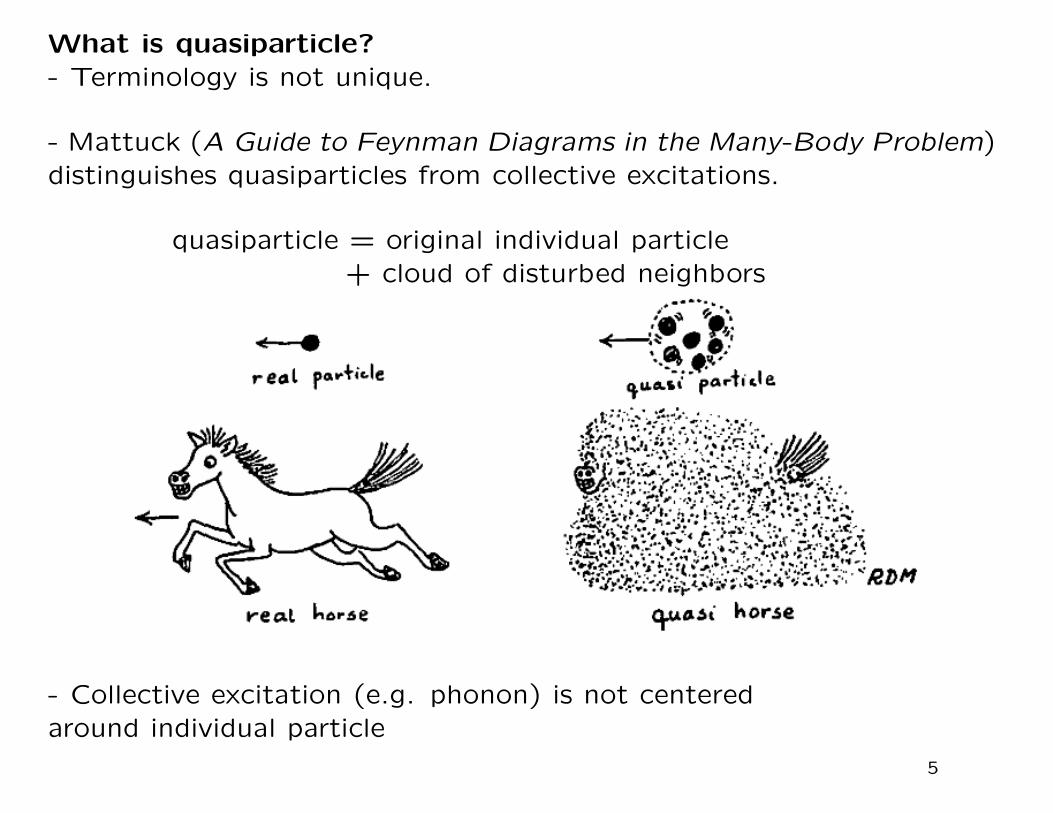
What is quasiparticle?- Terminology is not unique.

- Mattuck (A Guide to Feynman Diagrams in the Many-Body Problem)distinguishes quasiparticles from collective excitations.

quasiparticle = original individual particle+ cloud of disturbed neighbors

- Collective excitation (e.g. phonon) is not centeredaround individual particle

5

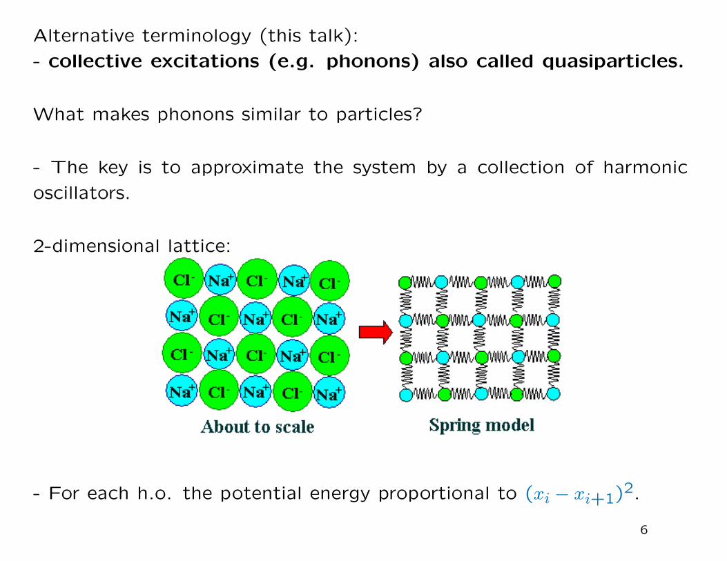
Alternative terminology (this talk):

- collective excitations (e.g. phonons) also called quasiparticles.

What makes phonons similar to particles?

- The key is to approximate the system by a collection of harmonic

oscillators.

2-dimensional lattice:

- For each h.o. the potential energy proportional to (xi − xi+1)2.

6

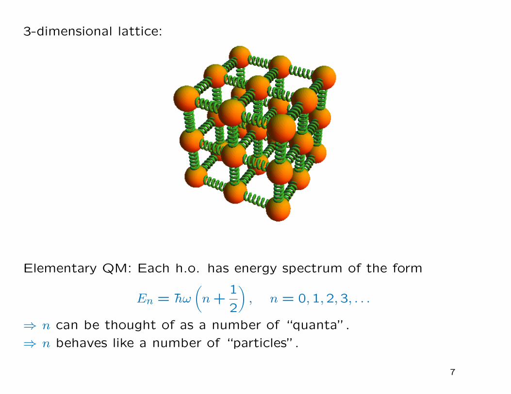
3-dimensional lattice:

Elementary QM: Each h.o. has energy spectrum of the form

En = hω

(n+

1

2

), n = 0,1,2,3, . . .

⇒ n can be thought of as a number of “quanta”.

⇒ n behaves like a number of “particles”.

7

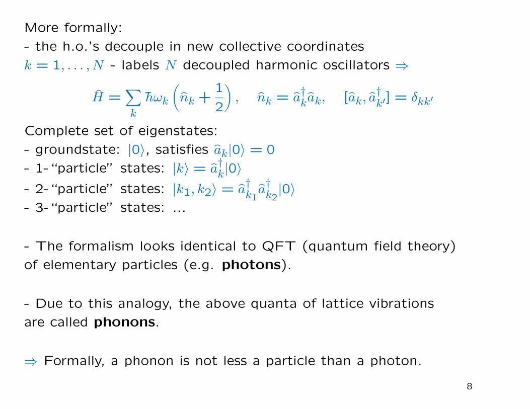
More formally:

- the h.o.’s decouple in new collective coordinates

k = 1, . . . , N - labels N decoupled harmonic oscillators ⇒

H =∑k

hωk

(nk +

1

2

), nk = a

†kak, [ak, a

†k′] = δkk′

Complete set of eigenstates:

- groundstate: |0⟩, satisfies ak|0⟩ = 0

- 1-“particle” states: |k⟩ = a†k|0⟩

- 2-“particle” states: |k1, k2⟩ = a†k1a†k2|0⟩

- 3-“particle” states: ...

- The formalism looks identical to QFT (quantum field theory)

of elementary particles (e.g. photons).

- Due to this analogy, the above quanta of lattice vibrations

are called phonons.

⇒ Formally, a phonon is not less a particle than a photon.

8

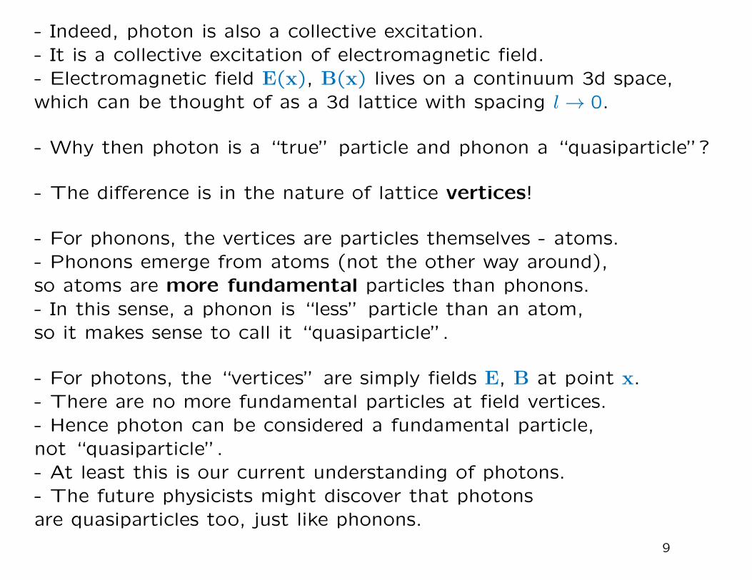
- Indeed, photon is also a collective excitation.- It is a collective excitation of electromagnetic field.- Electromagnetic field E(x), B(x) lives on a continuum 3d space,which can be thought of as a 3d lattice with spacing l → 0.

- Why then photon is a “true” particle and phonon a “quasiparticle”?

- The difference is in the nature of lattice vertices!

- For phonons, the vertices are particles themselves - atoms.- Phonons emerge from atoms (not the other way around),so atoms are more fundamental particles than phonons.- In this sense, a phonon is “less” particle than an atom,so it makes sense to call it “quasiparticle”.

- For photons, the “vertices” are simply fields E, B at point x.- There are no more fundamental particles at field vertices.- Hence photon can be considered a fundamental particle,not “quasiparticle”.- At least this is our current understanding of photons.- The future physicists might discover that photonsare quasiparticles too, just like phonons.

9

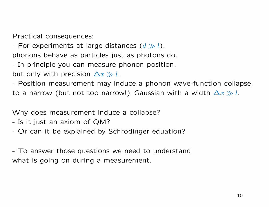
Practical consequences:

- For experiments at large distances (d≫ l),

phonons behave as particles just as photons do.

- In principle you can measure phonon position,

but only with precision ∆x≫ l.

- Position measurement may induce a phonon wave-function collapse,

to a narrow (but not too narrow!) Gaussian with a width ∆x≫ l.

Why does measurement induce a collapse?

- Is it just an axiom of QM?

- Or can it be explained by Schrodinger equation?

- To answer those questions we need to understand

what is going on during a measurement.

10

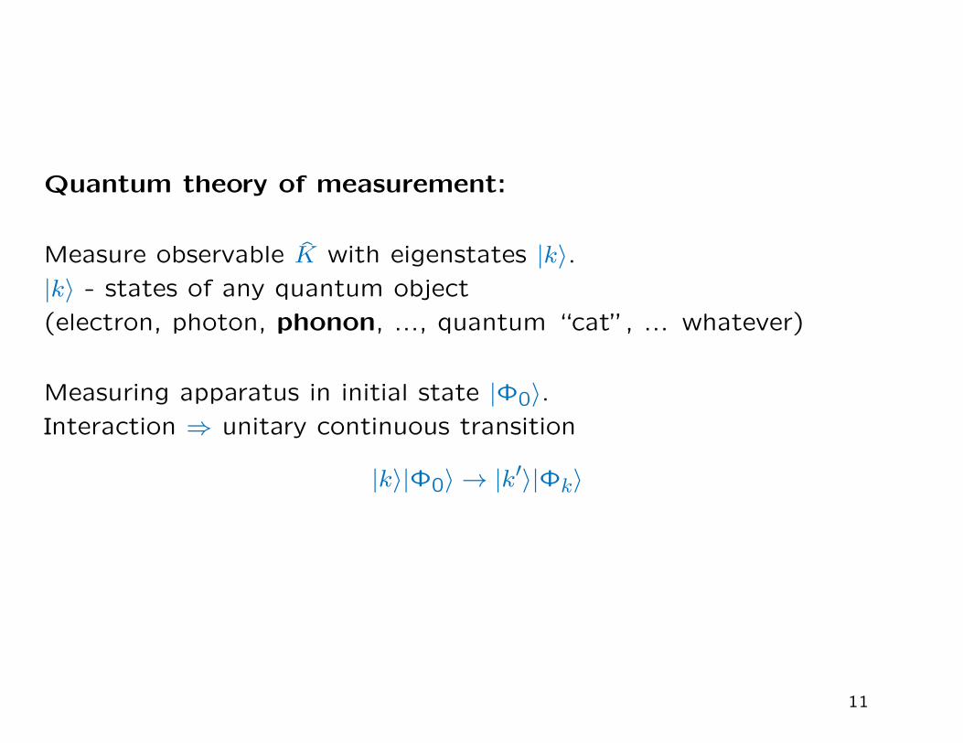
Quantum theory of measurement:

Measure observable K with eigenstates |k⟩.|k⟩ - states of any quantum object

(electron, photon, phonon, ..., quantum “cat”, ... whatever)

Measuring apparatus in initial state |Φ0⟩.Interaction ⇒ unitary continuous transition

|k⟩|Φ0⟩ → |k′⟩|Φk⟩

11

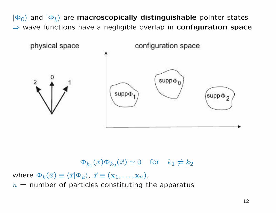
|Φ0⟩ and |Φk⟩ are macroscopically distinguishable pointer states

⇒ wave functions have a negligible overlap in configuration space

Φk1(x)Φk2(x) ≃ 0 for k1 = k2

where Φk(x) ≡ ⟨x|Φk⟩, x ≡ (x1, . . . ,xn),

n = number of particles constituting the apparatus

12

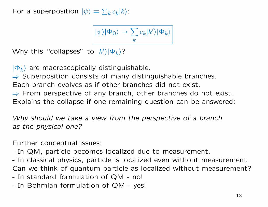
For a superposition |ψ⟩ =∑k ck|k⟩:

|ψ⟩|Φ0⟩ →∑k

ck|k′⟩|Φk⟩

Why this “collapses” to |k′⟩|Φk⟩?

|Φk⟩ are macroscopically distinguishable.⇒ Superposition consists of many distinguishable branches.Each branch evolves as if other branches did not exist.⇒ From perspective of any branch, other branches do not exist.Explains the collapse if one remaining question can be answered:

Why should we take a view from the perspective of a branchas the physical one?

Further conceptual issues:- In QM, particle becomes localized due to measurement.- In classical physics, particle is localized even without measurement.Can we think of quantum particle as localized without measurement?- In standard formulation of QM - no!- In Bohmian formulation of QM - yes!

13

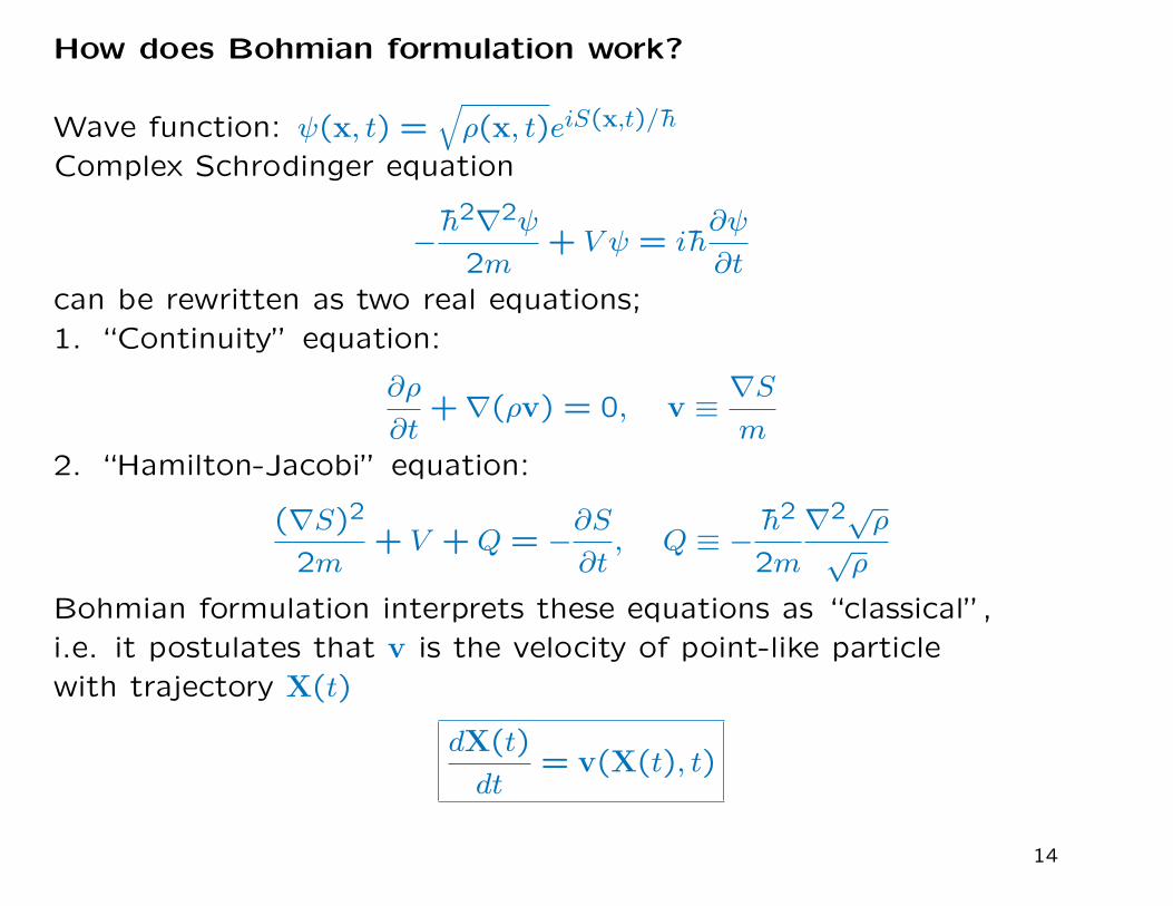
How does Bohmian formulation work?

Wave function: ψ(x, t) =√ρ(x, t)eiS(x,t)/h

Complex Schrodinger equation

−h2∇2ψ

2m+ V ψ = ih

∂ψ

∂tcan be rewritten as two real equations;1. “Continuity” equation:

∂ρ

∂t+∇(ρv) = 0, v ≡

∇Sm

2. “Hamilton-Jacobi” equation:

(∇S)2

2m+ V +Q = −

∂S

∂t, Q ≡ −

h2

2m

∇2√ρ√ρ

Bohmian formulation interprets these equations as “classical”,i.e. it postulates that v is the velocity of point-like particlewith trajectory X(t)

dX(t)

dt= v(X(t), t)

14

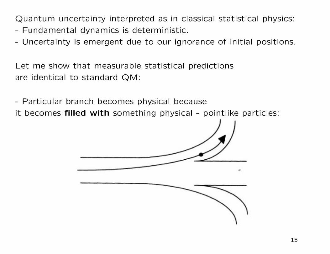
Quantum uncertainty interpreted as in classical statistical physics:

- Fundamental dynamics is deterministic.

- Uncertainty is emergent due to our ignorance of initial positions.

Let me show that measurable statistical predictions

are identical to standard QM:

- Particular branch becomes physical because

it becomes filled with something physical - pointlike particles:

15

⇒ Filling entity is described by position

X ≡ (X1, . . . ,Xn)

n = number of particles constituting the apparatus.

⇒ Apparatus made of pointlike particles.

- If apparatus particles are real and pointlike,does it make sense to assume that so are other particles?

X1, . . . ,Xn,Xn+1, . . . ,XN

N = total number of particles in the laboratory

Probability density of particle positions:

ρ(x1, . . . ,xN , t) = |Ψ(x1, . . . ,xN , t)|2

- cannot be tested in practice(one cannot observe all particles in the whole laboratory).

- One really observes macroscopic observable describingthe measuring apparatus.

16

⇒ Phenomenologically more interesting is apparatus probability density

ρ(appar)(x1, . . . ,xn, t) =∫d3xn+1 · · · d3xN ρ(x1, . . . ,xn,xn+1, . . . ,xN , t)

⇒

ρ(appar)(x) ≃∑k

|ck|2 |Φk(x)|2

⇒ Probability to find the apparatus particles in the support of Φk(x):

pk =∫supp Φk

d3nx ρ(appar)(x) ≃ |ck|2

- this is the Born rule.

⇒ We derived Born rule in arbitrary k-basis

from assumption of Born rule in position basis.

⇒ It is crucial that apparatus particles exist

and have the quantum probability distribution.

- not so important whether positions

of the observed system (photon, phonon, ...) exist.

17

Bohmian formulation used in two ways:

- As a fundamental interpretation of QM (alternative to Copenhagen):

assumes that particle trajectories really exist in Nature.

- As a practical tool for computations (e.g. Xavier Oriols et al).

- Bohmian formulation often used for electrons.

- Can Bohmian formulation be used for phonons?

As a fundamental interpretation of phonons:

- No, because we know that phonon is not a fundamental particle,

but emerges from collective motion of atoms.

As a practical tool for phonon computations:

- Yes, because

(when phonon can be described by a Schrodinger-like equation)

Bohmian formulation will lead to same measurable predictions

as standard theory of phonons.

18

Final warnings:

- Be careful not to take seriously the phonon theory

(either standard or Bohmian) at small distances.

- Take phonons seriously only at distances

much larger than the interatomic distance.

- At smaller distances reformulate your problem

in terms of more fundamental particles (atoms, electrons, photons, ...).

19

Part 2.

THE ORIGIN OF CASIMIR EFFECT

Vacuum Energy or van der Waals Force?

20

- Spectrum of h.o.

En = hω

(n+

1

2

)⇒ Energy of the ground state E0 = hω/2.- Is this energy physical?

- Standard answer - no, because we only measure energy differences.⇒ We can subtract this constant without changing physics

⇒ En = hωn

- On the other hand, often claimed in literaturethat Casimir effect is a counter-example.- Is Casimir effect evidence that vacuum energy is physical?

Casimir effect = attractive force between electrically neutral plates

Two explanations:1) vacuum energy of electro-magnetic field2) van der Waals force- Which explanation is correct?

21

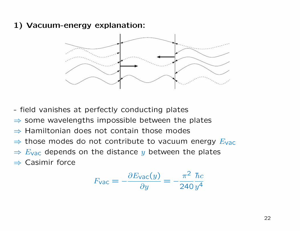
1) Vacuum-energy explanation:

- field vanishes at perfectly conducting plates

⇒ some wavelengths impossible between the plates

⇒ Hamiltonian does not contain those modes

⇒ those modes do not contribute to vacuum energy Evac

⇒ Evac depends on the distance y between the plates

⇒ Casimir force

Fvac = −∂Evac(y)

∂y= −

π2

240

hc

y4

22

Advantages:

- calculation relatively simple

- presented in many textbooks

Disadvantages:

- Electromagnetic forces are forces between charges,

but where are the charges?

- Force originates from boundary conditions, but microscopic origin

of boundary conditions not taken into account.

⇒ Vacuum-energy explanation is not a fully microscopic explanation.

Those disadvantages avoided by van der Waals force approach.

23

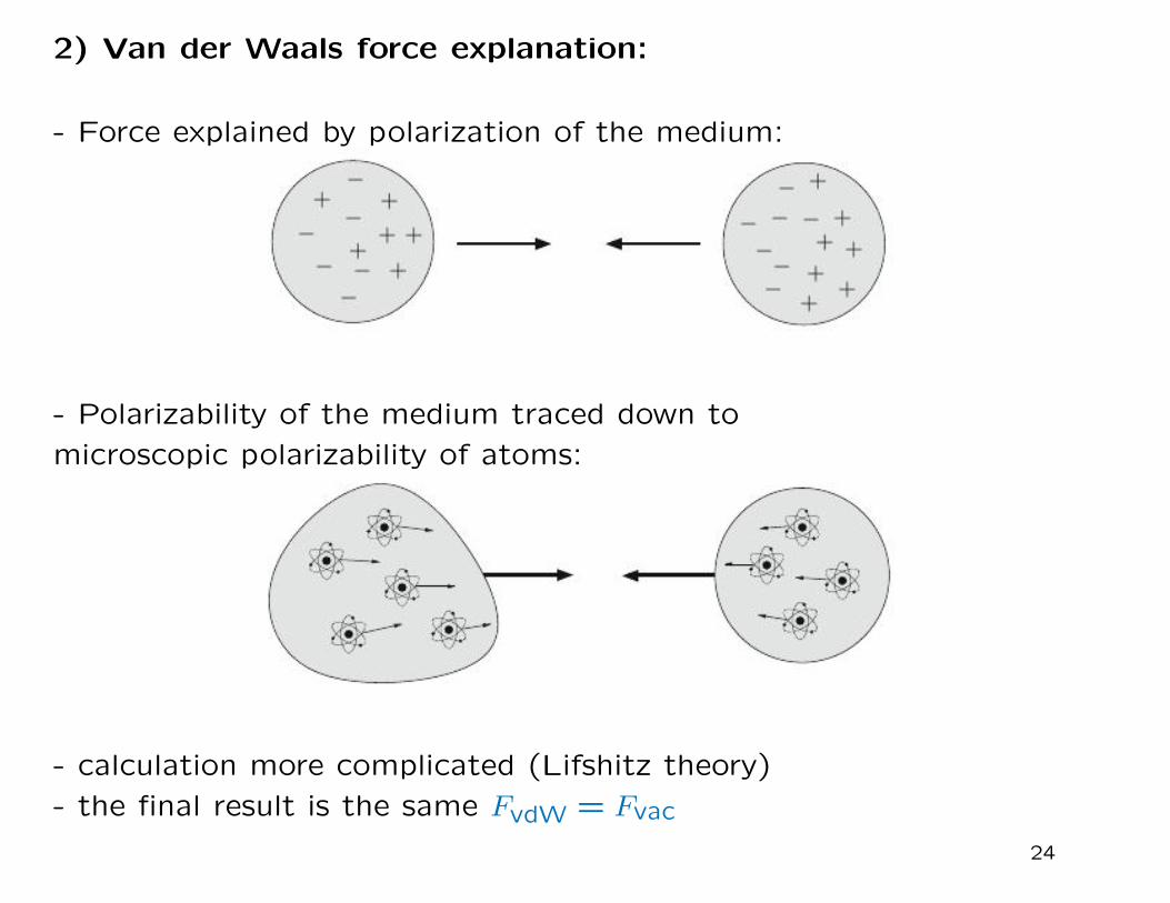
2) Van der Waals force explanation:

- Force explained by polarization of the medium:

- Polarizability of the medium traced down to

microscopic polarizability of atoms:

- calculation more complicated (Lifshitz theory)

- the final result is the same FvdW = Fvac

24

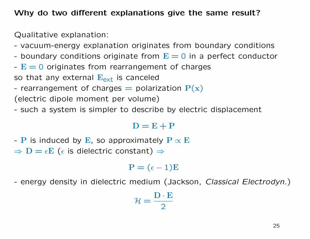
Why do two different explanations give the same result?

Qualitative explanation:

- vacuum-energy explanation originates from boundary conditions

- boundary conditions originate from E = 0 in a perfect conductor

- E = 0 originates from rearrangement of charges

so that any external Eext is canceled

- rearrangement of charges = polarization P(x)

(electric dipole moment per volume)

- such a system is simpler to describe by electric displacement

D = E+P

- P is induced by E, so approximately P ∝ E

⇒ D = ϵE (ϵ is dielectric constant) ⇒

P = (ϵ− 1)E

- energy density in dielectric medium (Jackson, Classical Electrodyn.)

H =D · E2

25

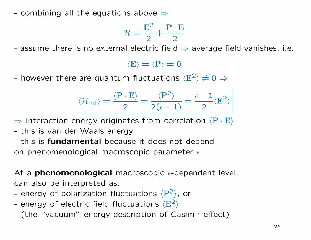
- combining all the equations above ⇒

H =E2

2+

P · E2

- assume there is no external electric field ⇒ average field vanishes, i.e.

⟨E⟩ = ⟨P⟩ = 0

- however there are quantum fluctuations ⟨E2⟩ = 0 ⇒

⟨Hint⟩ =⟨P · E⟩

2=

⟨P2⟩2(ϵ− 1)

=ϵ− 1

2⟨E2⟩

⇒ interaction energy originates from correlation ⟨P · E⟩- this is van der Waals energy- this is fundamental because it does not dependon phenomenological macroscopic parameter ϵ.

At a phenomenological macroscopic ϵ-dependent level,can also be interpreted as:- energy of polarization fluctuations ⟨P2⟩, or- energy of electric field fluctuations ⟨E2⟩(the “vacuum”-energy description of Casimir effect)

26

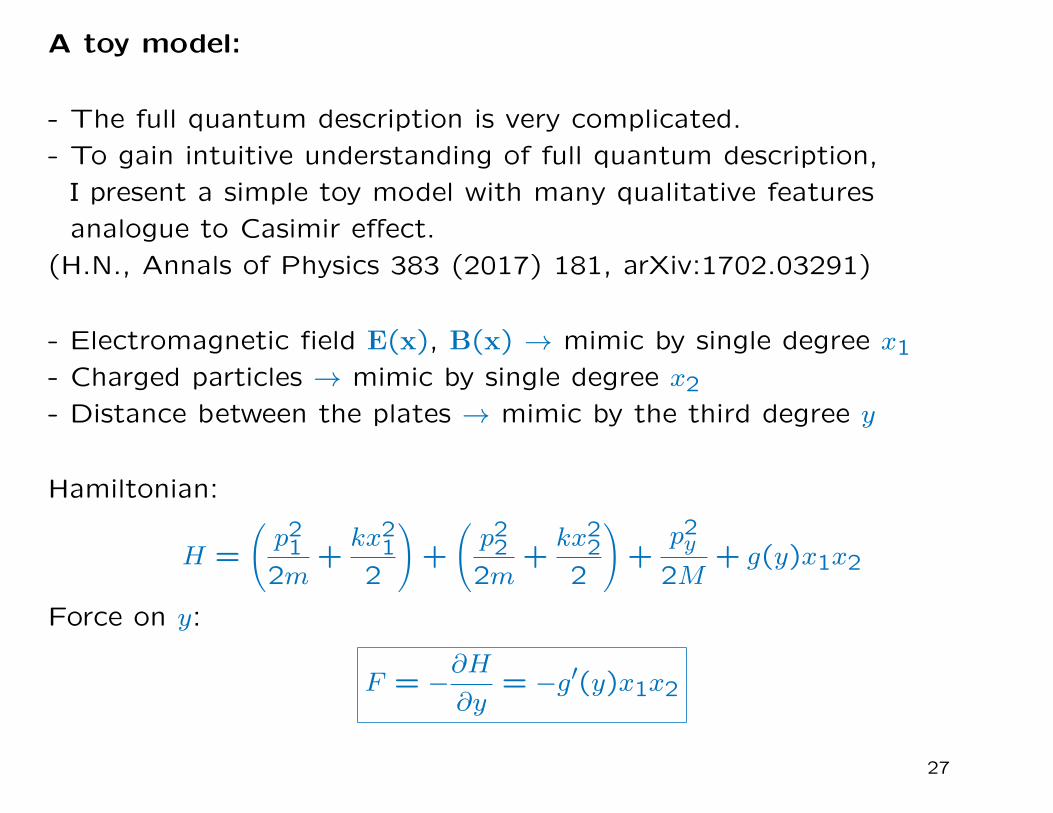
A toy model:

- The full quantum description is very complicated.

- To gain intuitive understanding of full quantum description,

I present a simple toy model with many qualitative features

analogue to Casimir effect.

(H.N., Annals of Physics 383 (2017) 181, arXiv:1702.03291)

- Electromagnetic field E(x), B(x) → mimic by single degree x1- Charged particles → mimic by single degree x2- Distance between the plates → mimic by the third degree y

Hamiltonian:

H =

(p212m

+kx212

)+

(p222m

+kx222

)+

p2y

2M+ g(y)x1x2

Force on y:

F = −∂H

∂y= −g′(y)x1x2

27

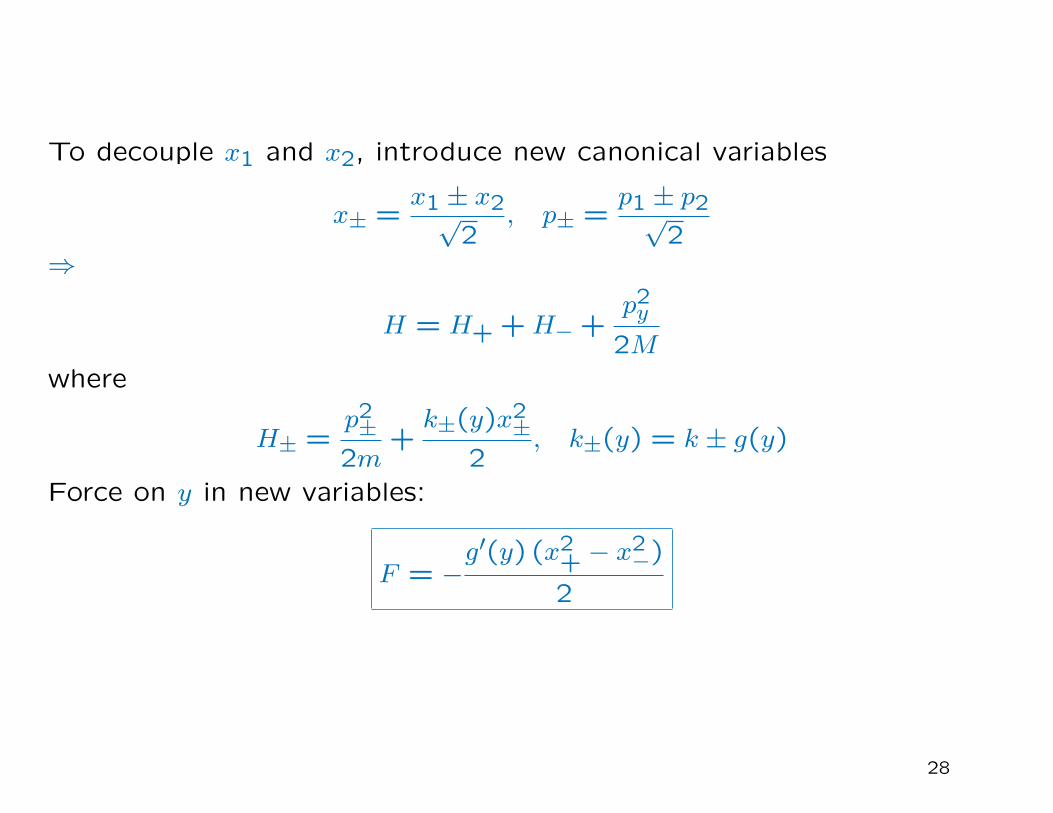
To decouple x1 and x2, introduce new canonical variables

x± =x1 ± x2√

2, p± =

p1 ± p2√2

⇒

H = H+ +H− +p2y

2Mwhere

H± =p2±2m

+k±(y)x2±

2, k±(y) = k ± g(y)

Force on y in new variables:

F = −g′(y) (x2+ − x2−)

2

28

To quantize the theory we make an approximation:

- treat y as a classical background

⇒ quantize only the effective Hamiltonian

H(eff) = H+ +H−

⇒ two (quantum) uncoupled harmonic oscillators

H± = hΩ±(y)(a†±a± +

1

2

), Ω2

±(y) =k ± g(y)

m

effective vacuum a±|0⟩ = 0 ⇒

E(eff)vac = ⟨0|H(eff)|0⟩ =

hΩ+(y)

2+hΩ−(y)

2⇒ Casimir-like force

F = −∂E

(eff)vac

∂y= −

hΩ′+(y)

2−hΩ′

−(y)

2=

− hg′(y)4mΩ+(y)

+hg′(y)

4mΩ−(y)

- Not clear how is this quantum force related to the classical force?

29

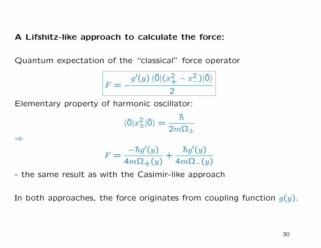
A Lifshitz-like approach to calculate the force:

Quantum expectation of the “classical” force operator

F = −g′(y) ⟨0|(x2+ − x2−)|0⟩

2

Elementary property of harmonic oscillator:

⟨0|x2±|0⟩ =h

2mΩ±⇒

F =− hg′(y)4mΩ+(y)

+hg′(y)

4mΩ−(y)

- the same result as with the Casimir-like approach

In both approaches, the force originates from coupling function g(y).

30

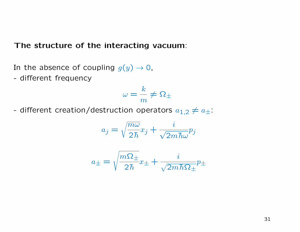
The structure of the interacting vacuum:

In the absence of coupling g(y) → 0,

- different frequency

ω =k

m= Ω±

- different creation/destruction operators a1,2 = a±:

aj =√mω

2 hxj +

i√2mhω

pj

a± =

√mΩ±2 h

x± +i√

2mhΩ±p±

31

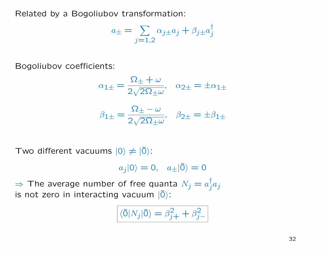
Related by a Bogoliubov transformation:

a± =∑

j=1,2

αj±aj + βj±a†j

Bogoliubov coefficients:

α1± =Ω± + ω

2√2Ω±ω

, α2± = ±α1±

β1± =Ω± − ω

2√2Ω±ω

, β2± = ±β1±

Two different vacuums |0⟩ = |0⟩:

aj|0⟩ = 0, a±|0⟩ = 0

⇒ The average number of free quanta Nj = a†jaj

is not zero in interacting vacuum |0⟩:

⟨0|Nj|0⟩ = β2j+ + β2j−

32

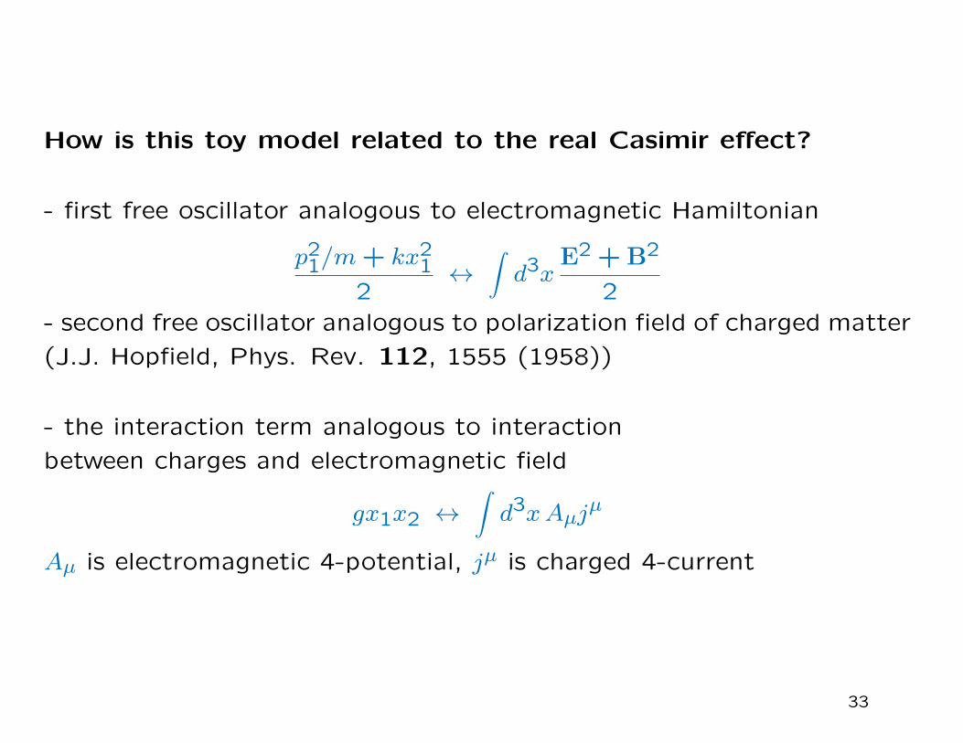
How is this toy model related to the real Casimir effect?

- first free oscillator analogous to electromagnetic Hamiltonian

p21/m+ kx212

↔∫d3x

E2 +B2

2- second free oscillator analogous to polarization field of charged matter

(J.J. Hopfield, Phys. Rev. 112, 1555 (1958))

- the interaction term analogous to interaction

between charges and electromagnetic field

gx1x2 ↔∫d3xAµj

µ

Aµ is electromagnetic 4-potential, jµ is charged 4-current

33

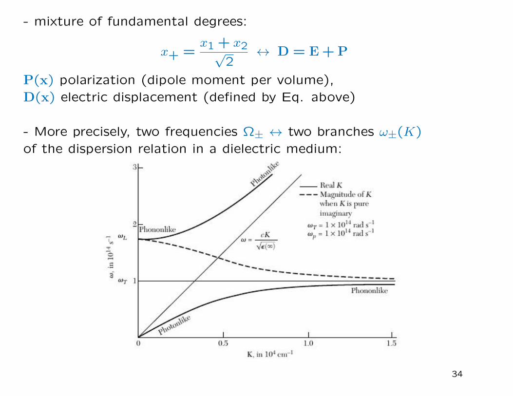
- mixture of fundamental degrees:

x+ =x1 + x2√

2↔ D = E+P

P(x) polarization (dipole moment per volume),D(x) electric displacement (defined by Eq. above)

- More precisely, two frequencies Ω± ↔ two branches ω±(K)of the dispersion relation in a dielectric medium:

34

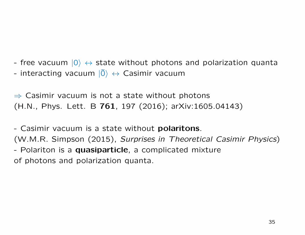
- free vacuum |0⟩ ↔ state without photons and polarization quanta

- interacting vacuum |0⟩ ↔ Casimir vacuum

⇒ Casimir vacuum is not a state without photons

(H.N., Phys. Lett. B 761, 197 (2016); arXiv:1605.04143)

- Casimir vacuum is a state without polaritons.

(W.M.R. Simpson (2015), Surprises in Theoretical Casimir Physics)

- Polariton is a quasiparticle, a complicated mixture

of photons and polarization quanta.

35

The final question: What is vacuum?

In physics, there are different definitions of the word “vacuum”:

1) - state without any particles

2) - state without photons

3) - state annihilated by some lowering operators ak|0⟩ = 0

4) - local minimum of a classical potential

5) - state with lowest possible energy (ground state)

- Casimir vacuum is only 3),

it has zero number of quasiparticles (polaritons).

- Casimir vacuum is not 5),

for otherwise Casimir force could not attract the plates

to a state of even lower energy.

36