Quasiperiodically forced dynamical systems with strange nonchaotic attractors

Physica 26D (1987) 277-294 North-Holland, Amsterdam

QUASIPERIODICALLY FORCED DYNAMICAL SYSTEMS WITH STRANGE NONCHAOTIC ATTRACTORS

Filipe J. ROMEIRAS a,b, Anders BONDESON c, Edward OTT a, Thomas M. ANTONSEN Jr, a and Celso GREBOGI a aLaboratory for Plasma and Fusion Energy Studies, University of Maryland, College Park, MD 20742, USA t~Permanent address: Centro de Electrodin~mica, Instituto Superior Tdcnico, 1096 Lisboa Codex, Portugal "Institute for Electromagnetic Field Theory, Chalmers University of Technology, S 41296 Grteborg, Sweden

Received 14October 1986

We discuss the existence and properties of strange nonchaotic attractors of quasiperiodically forced nonlinear dynamical systems. We do this by examining a particular model differential equation, ~ = c o s f f + ecos24~+f(t) , where f is a two-frequency quasiperiodic function of t. When e = 0 the analysis of the equation is facilitated since then it can be related to the Schr6dinger equation with quasiperiodic potential. We show that the equation does indeed exhibit strange nonchaotic attractors, and we consider the important question of whether these attractors are typical in the sense that they exist on a set of positive Lebesgue measure in parameter space. (The equation also exhibits two- and three-frequency quasiperiodic behavior.) We also show that the strange nonchaotic attractors have distinctive frequency spectrum; this property might make them experimentally observable.

1. Introduction

Recently attention has been given to a class of dissipative dynamical systems that typically exhibit a class of attractors that may be described as strange and nonchaotic (Grebogi et al. [1]).

Here the word strange refers to the geometrical structure of the attractor: a strange attractor is an attractor which is neither a finite set of points nor is it piecewise differentiable (that is, either a piecewise differentiable curve or surface, or a volume bounded by a piecewise differentiable closed surface).

The word chaotic refers to the dynamics of the orbits on the attractor: a chaotic attractor is one for which typical orbits have a positive Lyapunov exponent. This implies that nearby orbits diverge exponentially from one another with time and that the orbit depends sensitively on its initial condi- tions.

By a strange nonchaotic attractor we therefore mean an attractor which seems to be geometrically

strange but for which typical nearby orbits do not diverge exponentially with time.

An example of a strange nonchaotic attractor is exhibited by the one-dimensional quadratic map, xn+ x = C - x 2, at the point of accumulation of period doublings. The attractor is a Cantor set of dimension = 0.538 and the Lyapunov exponent for a typical orbit is zero (Grassberger [2]). Attrac- tors of the same type occur at the infinite number of C values representing points of accumulation of period doublings of orbits of period 2Np corresponding to the infinite number of periodic windows occurring as C is varied. Nevertheless these strange nonchaotic attractors only occupy a set of C values of zero Lebesgue measure. That is, if we were to pick a C value at random, the probabili ty of that value yielding a strange nonchaotic attractor would be zero. In this sense we say that this type of attractor is not typical of the quadratic map.

As another example, consider the circle-map, O,+ x = D + 0~ + k sin0, [mod 2vr], for parameter

0167-2789/87/$03.50 © Elsevier Science Publishers B.V. (North-Holland Physics Publishing Division)

278 F.J. Romeiras et al. / Quasiperiodically forced dynamical systems

values k = 1 (the critical case) and ~2 chosen to give irrational winding number. In this case the Lyapunov exponent is zero, and the density of orbit points p(O) is zero on a dense set of 0 [0,2~r]. Due to this behavior of p(0) one might call this nonchaotic attractor strange. Again, however, the measure in parameter space (k, ~2) where this occurs is zero, and hence this type of attractor is not typical for the circle map*.

On the other hand, examples of systems where strange nonchaotic attractors are typical, in the sense of occupying a set of positive Lebesgue measure in the parameter space, were given by Grebogi et al. [1]. They examined a particular class of maps of the general form

x.+ 1 = g ( x . , 0.), ( la)

0.+ 1 = 0. + 2vno[mod2~r], ( lb )

where g is a 2~r-periodic function of its second argument and ~ is an irrational number**. In the paper of Grebogi et al. 0. was always taken to be a scalar while two cases were considered for x . , g: in case (1) x . , g were scalars and eq. (la) was taken to be of the form

x.+ 1 = 2~ (tanh x . ) cos 0.;

in case (ii) x . = (u. , v.) and g = (gl, g2) were two-dimensional vectors, and eq. ( la) was taken to be of the form

0] [ Un+l 1 + Un v.

× - s inO. cosO. v. "

In case (i) it was shown that the map exhibits a strange nonchaotic attractor with one negative

*For a third example, also with zero measure in parameter space, occurring for a system of the form of eqs. ( la , b), below, see fig. 6 of Sethna and Siggia [3].

**Equations of this form have also been investigated from other points of view by Sethna and Siggia [3] and by Kaneko [4].

Lyapunov exponent (the other, corresponding to eq. (lb), is trivially zero) for all X in the range IX[ > 1. In case (ii) it was shown that the attractor is also strange with two negative Lyapunov exponents (again the third is trivially zero) for all X above some critical value Xc(V ). The important result is the existence of strange nonchaotic attractors on a set of positive measure in parameter space.

Maps of the form (1) may be obtained from two-frequency quasiperiodically forced nonlinear systems (see section 2). It might therefore be sus- pected that such nonlinear systems can exhibit strange nonchaotic attractors for a positive measure of the parameter space. Off hand, however, it is not at all clear that this suspicion will be fulfilled, since the functions g(x , , 0,) (eq. (la)) used by Grebogi et al. [1] are highly artificial and were specifically constructed to demonstrate the possibility of strange nonchaotic attractors with positive measure in parameter space. Thus we cannot decide, on the basis of the work by Grebogi et al. [1], what the situation will be for quasiperiodically forced systems that are likely to arise in applications.

It is the aim of the present paper to discuss the existence and the properties of strange nonchaotic attractors of dynamical systems forced at two incommensurate frequencies by examining a specific model given by the non-autonomous first order differential equation

dq~ - cos ¢ + ecos2¢ + f ( t ) , (2a) dt

where f is two-frequency quasiperiodic (that is, f ( t ) =f(~oxt, ¢02t), where f is 2~r-periodic in both its arguments and o~l/w 2 is irrational) and e is a variable parameter. In our study f was actually taken to be of the form

f ( t ) = K + V(cos w,t + cos wzt), (28)

where w 1 = ½(v~- - 1) and w 2 = 1 were kept fixed while K, V were allowed to vary. Equations of this type are perhaps the simplest ordinary differential equations yielding a strange attractor.

F.J. Romeiras et al./ Quasiperiodically forced dynamical systems 279

Specifically we are primarily interested in (i) the question of parameter space measure (typicality), posed above, and (ii) in elucidating possible power spectral signatures of these attractors. (We believe that the signature we shall discuss may be a useful

diagnostic in experiments.)

In the special case e = 0, eq. (2) can be regarded as a simplified form of the well-known equation of the damped forced pendulum

d2tib + dq, i2 2 d t : v --dt- + sin~? = f ( t ) , (3)

corresponding to strong damping and forcing (so that the inertial term d2ep/dt 2 can be neglected).

Eq. (3) has also been extensively used as a model

of the current driven Josephson junction (see Gwinn and Westervelt [5], Kautz and MacFarlane [6], and references therein). The existence of

strange nonchaotic attractors for eq. (3) will be considered in a separate publication (Romeiras and Ott [7]).

Again in the case e = 0, eq. (2) can be related by the so-called Priifer transformation of the depen-

dent variable q~(t) ~ ~k(x), defined by

ei , t , _ ~ ' / t ~ + ic + ' / ~ b - i c '

(see Johnson and Moser [8]) with the change of independent variable t ~ x, defined by

J0"( ] x = ~ t + E ) d E ,

to the linear " t ime independent" Schrrdinger equation

~ b " + k 2 ( x ) ~ b = O , with k : = c2f/--~+ 1 1"

understanding the behavior of the solutions of eq. (2). This has been done by Bondeson et al. [11] where some of the results presented in this paper were first briefly described.

The fact that the case e = 0 allows a reduction

to the Schrrdinger equation, although convenient for analysis, also means that we are dealing with a special case whose properties might differ qualitatively from those typical of equations of the gen-

eral form

d e d-7 = gn (~ ' t ) , (4)

where gn(0, t) is periodic in ~ and two-frequency

quasiperiodic in t, and , / = (*/1, ~2, . . . , */N) denotes the parameters of the system. Thus we also investigate the e 4= 0 case, since the Priifer transformation does not apply, and hence more gener-

ally applicable qualitative behavior should occur*. Indeed, as shown in sections 3 and 4, the e #: 0

case has many more resonances than the e = 0

case**. The plan of this paper is as follows. In section 2

we present the detailed results of the numerical study of eq. (2) in the case e = 0. In sections 3 and 4 we discuss the case e ~ 0. Finally in section 5 we summarize the main conclusions of the study. For e = 0 we find that there are indeed strange nonchaotic attractors for a positive measure of parameters. Thus such attractors are typical for this system. There is, however, an important difference as compared to the situations occurring in Grebogi et al. [1]). Namely, parameter values corresponding to strange nonchaotic attractors of eq. (2) with e = 0 do not occur on an interval, but rather lie on

a Cantor set of positive measure. In the case e 4: 0, our numerical results strongly suggest that the

Here the prime denotes differentiation with re- spect to x and c is an arbitrary constant. Since f is quasiperiodic in t, k 2 will be quasiperiodic in x. Thus the theory of the Schr/Sdinger equation with quasiperiodic potential (see the reviews by Simon [9] and Souillard [10]) can be used to aid in

*In the e term, in place of cos(2q~) we could have used some other smooth 2~r-periodic [unction of ~,.

**For e = 0 we shall see that the winding number plateaus (resonances) occur at W= l% + m%, whereas for e 4:0 they occur at W= ( / / / n )~o 1 + (m/n)oa2, where W is the winding numbers and /, m, n are integers. The latter case is to be expected in the general context of equations of the form (4), while the former case is specific to eq. (2) with e = 0.

280 F.J. Romeiras et al. / Quasiperiodically forced dynamical systems

same situation also applies, although we have no direct analytical support (the SchrSdinger equation correspondence only applies for e = 0). Thus we believe that strange nonchaotic attractors are typical for quasiperiodically forced systems of the form (4), where by "typical" we mean that they occur on a set of positive measure in parameter space.

The winding number, W, is defined by

W = lim O ( T ) - O ( 0 ) T ~ o ¢ T

It represents the mean angular frequency of the solution.

The surface of section plot is obtained by strobing the solution of eq. (4) at times

2. The case e = 0 2"/7"

t . = - - n + t o , (6) 09 2

2.1. Characterization of attractors

Before starting with the presentation and discussion of the numerical results we introduce the main quantities used to characterize the attractors, namely, the Lyapunov characteristic exponent, the winding number, the surface of section plot and the frequency spectrum.

The Lyapunov characteristic exponent, A, for an orbit q,(t) of eq. (4) is defined by [12]

1 I~(~)(T)I A = lim -~ In r - ~ Iq,°)(0)l

where q,o) denotes the solution of the equation of first variation

dOO) agn dt ---A(t)th(1)' A ( t ) = - - ~ ( ~ ( t ) , t) . (5)

By using the explicit form of the solution of eq. (5) we can also write

1/0T A = lim ~ A ( t ) d t . T ~ o o

The Lyapunov exponent represents the mean ex- ponential rate of divergence of two initially close trajectories*.

*The nonautonomous eq. (4) can be written as an autonomous system of three first order equations of the form dq~/dt = gn(q', qq, +z), d f f l / d t = wl, dff: /dt = o~ 2. In this case there are three Lyapunov exponents. However, two of them, corresponding to the second and third equations, are zero; the third is A given above.

where n is an integer, and plotting

ft. = O(t . ) [mod2~r] , (7)

versus

On = 09at, [mod 2~r ]. (8)

The solution of eq. (4) thus generates a discrete time map

d n+ l = G( t n, On),

0,,+1 = On + 2 r09[mod2 r],

(9a)

(9b)

where 09 = 0 9 1 / 0 9 2 - The function G must be invert- ible for q, since eq. (4) can also be solved going backward in time.

The frequency spectrum was obtained in the following way: (1) From the sequence { q,. }.=0, M- 1 obtain the new sequence (S.}.~0. M-1- S . = h.P(ep.), where P is some smooth 2~r-periodic function (which was actually taken to be P ( ~ ) = cosq0 and h. = ½(1- cos2~rn/M); the multi- plication by h. corresponds to the so-called Hanning's method of leakage reduction and is a means of smoothing out spurious spectral features introduced by the finite duration of the time series. (ii) Calculate the discrete Fourier transform {Sk)k=O,M_ 1 of the sequence (S,},=O,M_ 1 defined by

S k= ~_, s , exp - i - ~ - k n , k = O , M - 1 , n = O

(10)

F.J. Romeiras et aL / Quasiperiodically forced dynamical systems 281

o e " '

o. L o.,

0.0 -

0.8 1.0 1.2 1.4 1.6 1.8 K

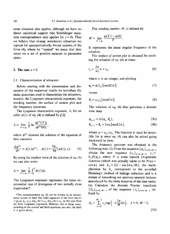
Fig. 1. Diagram of the K-V-plane showing regions where A < 0 (hatched) or A = 0 (blank). The curve denoted by (C) is the critical curve. The curve denoted by (W) is the curve of constant winding number W = 0.9277... along which the orbits of fig. 8 and the corresponding spectra of fig. 9 were calculated [~ = o . o ] .

by using a Fast Fourier Transform algorithm. (See Brigham [13] as a general reference on these topics and Powell and Percival [14].)

The differential system (4)-(5) was integrated by using a 4th order Runge-Kutta method with 32 time steps per period of the cost driver. The number of driver periods, N, was taken between 2 x 103 and 4 x 105, depending on the cir- cumstances. For the FFT algorithm M = 216 points were used. The computations were carried out on a CRAY X-MP machine; by using the vector mode operation (see Petersen [15]), when possible, a 15 fold increase in speed was achieved.

In the remainder of this section we present and discuss the numerical results for eq. (2) with e = 0.

2.2. Lyapunov exponents and winding numbers

Fig. 1 shows a diagram of the K-V-plane giving regions where A is negative (hatched) or zero (blank). The criterion for negative Lyapunov exponent used in this figure is A < - 1 0 -4. The diagram was obtained by taking a grid with 201 values of K and 66 values of V; the integration of the differential system was taken over a variable number of driver periods going from N = 2 X 103 for most cases up to N = 16 X 103 for the more slowly converging ones. The diagram exhibits a

b,

0.0

- 0 . 2

- 0 . 4

-0 .6

i T i r i i , i z i

- 0 . 8 i

- I '01 . . . . . . . . .

0.6 0.8 1.0 1.2 K

2.O

1.6

1.2 W

0.8

0.4

0.0

1.4 1.6 1.8

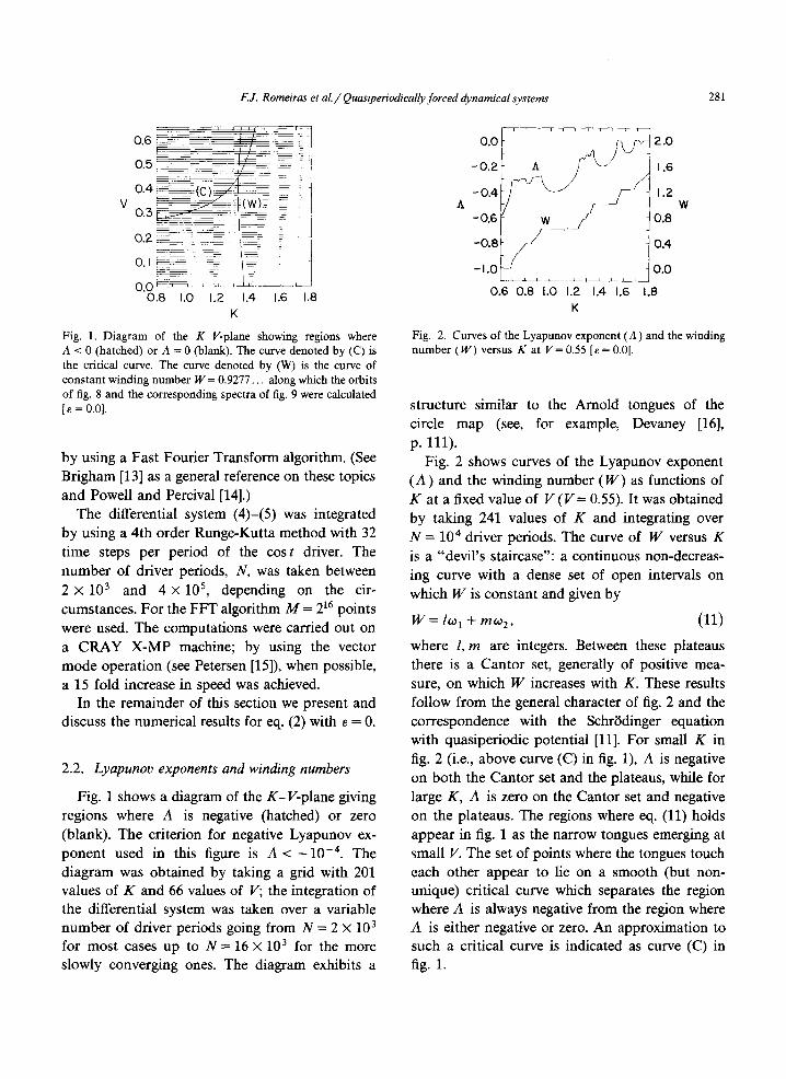
Fig. 2. Curves of the Lyapunov exponent (A) and the winding number (W) versus K at V= 0.55 [e = 0.0].

structure similar to the Arnold tongues of the circle map (see, for example, Devaney [16], p. 111).

Fig. 2 shows curves of the Lyapunov exponent (A) and the winding number (W) as functions of K at a fixed value of V ( V = 0.55). It was obtained by taking 241 values of K and integrating over N---- 10 4 driver periods. The curve of W versus K is a "devil's staircase": a continuous non-decreasing curve with a dense set of open intervals on which W is constant and given by

W = lw i + row2, (11)

where l, m are integers. Between these plateaus there is a Cantor set, generally of positive measure, on which W increases with K. These results follow from the general character of fig. 2 and the correspondence with the Schrtdinger equation with quasiperiodic potential [11]. For small K in fig. 2 (i.e., above curve (C) in fig. 1), A is negative on both the Cantor set and the plateaus, while for large K, A is zero on the Cantor set and negative on the plateaus. The regions where eq. (11) holds appear in fig. 1 as the narrow tongues emerging at small V. The set of points where the tongues touch each other appear to lie on a smooth (but non- unique) critical curve which separates the region where A is always negative from the region where A is either negative or zero. An approximation to such a critical curve is indicated as curve (C) in fig. 1.

282 F.J. Romeiras et a l . / Quasiperiodically forced dynamical systems

Table 1

Analogy with Lyapunov solutions of

Case Winding number exponent Type of attractor SchrSdinger eq. Fig.

A W4: lw 1 + m w 2 A = 0 3-freq. quasiperiodic extended 3a B W = l~o 1 + rn,% A < 0 2-freq. quasiperiodic stop band 3b C W =g lto I + rn~02 A < 0 strange nonchaotic localized 3c

2.3. Surface of section characterization

The three distinct combinations of winding numbers (either satisfying eq. (11) or not) and Lyapunov exponents (either negative or zero) give rise to surface of section plots with qualitatively different characteristics- see table I. In terms of

the analogy with the SchriSdinger equation [11], cases A, B, and C correspond to extended, stop band and Anderson localized solutions, respectively (see Aubry and Andre [17], as well as refs. [9, 10], for a discussion of Anderson localization in incommensurate lattices).

In case A, the three frequencies W, ~01 and ~0 2 are typically irrationally related, and eq. (2) will exhibit three-frequency quasiperiodic behavior. A typical orbit apparently generates a smooth den-

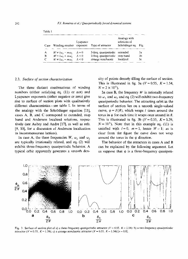
sity of points densely filling the surface of section. This is illustrated in fig. 3a (V= 0.55, K = 1.54, N = 2 × 105).

In case B, the frequency W is rationally related to ~o I and ~02 and eq. (2) will exhibit two-frequency quasiperiodic behavior. The attracting orbit in the surface of section lies on a smooth single-valued curve, ~ = F(0), which wraps l times around the torus in ~ for each time it wraps once around in 0. This is illustrated in fig. 3b (V= 0.55, K = 1.39, N = 105). Note that in this example eq. (11) is satisfied with / = 0 , m = 1, hence W = 1; as is clear from the figure the curve does not wrap around the torus in the ~ direction.

The behavior of the attractors in cases A and B can be explained by the following argument. Let us suppose that ~ is a three-frequency quasiperi-

~n 2"rr

. . . . . . . . 3 0.0 0.2 0.4 0.6 O.B 1.0 0.0 0.2 0.4. 0.6 0.8 1.0

a en b en c en 2"rr 2"tr 2"tr

: VI ' i ' ' I] 1

! I

L

Fig. 3. Surface of section plot of a) a three-frequency quasiperiodic attractor (V = 0.55, K = 1.54); b) a two-frequency quasiperiodic attractor ( V = 0.55, K = 1.39); c) a strange nonchaotic attractor ( V = 0.55, K = 1.34) [~ = 0.0].


odic function of t,

~ ( t ) = q ~ ( t ~ l t , 6~2t , Wt), (12)

where ~ is 2~r-periodic in each of its arguments and o~1, ~2, W are irrationally related. By strobing 4' at times t . given by (6) we obtain

~n ~ ~ ( tn) = @ ( t O l t n , td2tn, Wt,),

or, using the periodicity of ~ in its second argument

+. = Jo, wt . ) . (13)

the existence of the relationship q, = F(O) we ini- tialize a large number of points at a single initial O value but with different initial q~ values and find that after a large number of iterates N, say, all the orbits are attracted to a single value q'N; (ii) that q~ = F(8) cannot be a continuous curve follows from the fact that the winding number is irrationally related to ~1, 0~2; (iii) finally, that q, = F(8) is discontinuous everywhere follows from the fact that the 8 map is ergodic. An example of a strange nonchaotic attractor is given in fig. 3c (V = 0.55, K = 1.34, N = 2 x 105; the corresponding Lyapunov exponent is A = -0.07167).

If we now introduce the variable 0, defined by (8) this expression can be written in the form

W o

2 where ~ is a new function which is 27r-periodic in both arguments. As the 0-map (eq. (9b)) is ergodic and W/oo~ is irrational this expression will generate an orbit that will densely fill up the whole surface of section. In the particular case of two- frequency quasiperiodic behavior we have W = 10~ x + mto 2 and therefore by substituting into (13) and using the periodicity of ¢~ in its third argument we obtain

~n = ~ ( O~ltn, 602t0 ' lO)ltn + m~%to),

o r

+.= F(0.),

where F is a new function which is 2~r-periodic. Hence, in this case the orbit will generate a single curve in the surface of section. Note that, since the original function ~ is smooth, F is also smooth. (For a detailed discussion of quasiperiodicity and attractors on a N-torus see Grebogi et al. [18].)

In case C the attractor is geometrically strange: there still is a functional relationship q~ = F(O) but the function F is discontinuous everywhere. This can be verified in the following way: (i) to verify

2.4. Frequency spectra

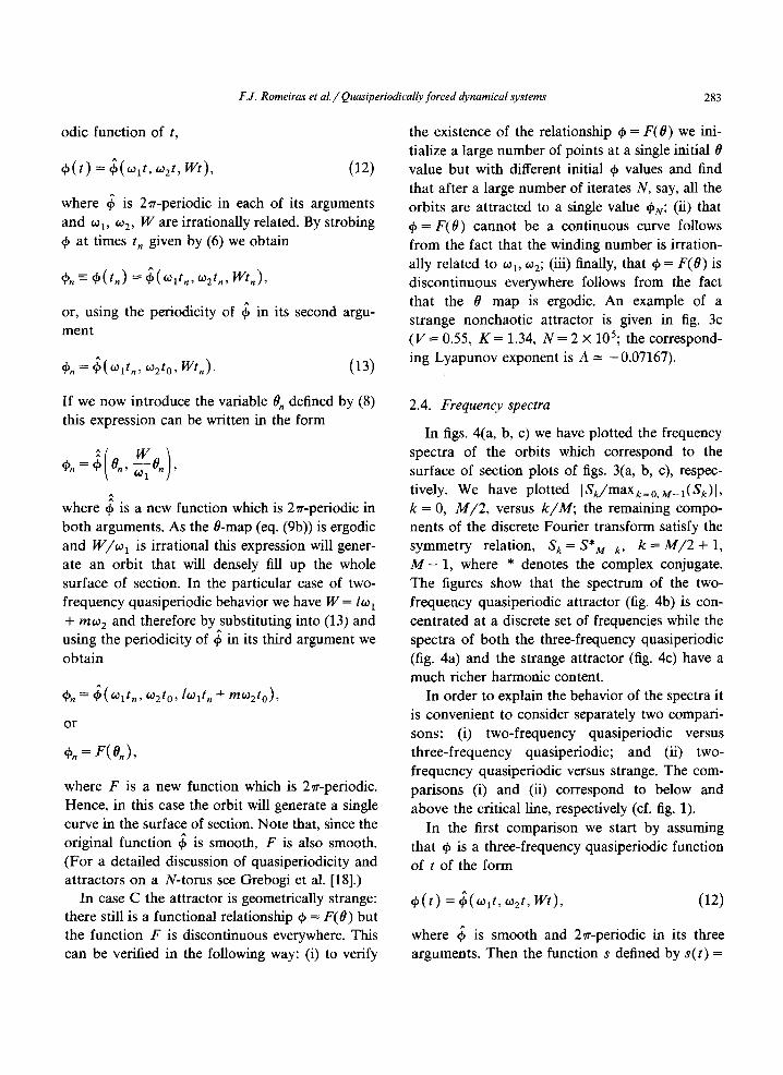
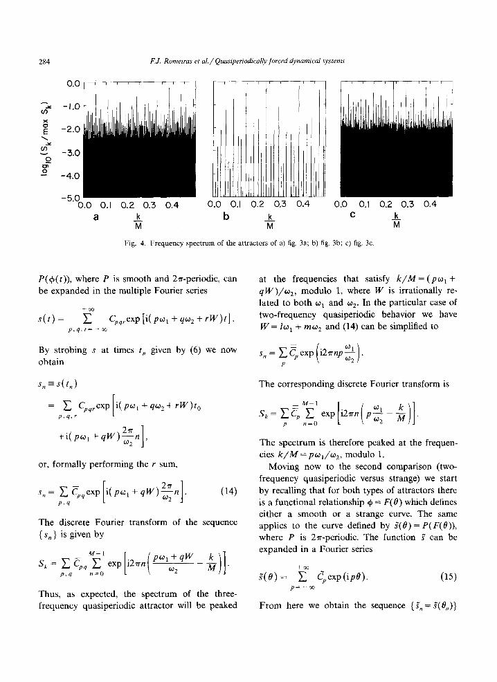
In figs. 4(a, b, c) we have plotted the frequency spectra of the orbits which correspond to the surface of section plots of figs. 3(a, b, c), respectively. We have plotted [S~/maXa=o.M_~(SDI, k = 0, M/2, versus k/M; the remaining components of the discrete Fourier transform satisfy the symmetry relation, S k = S*M_k, k = M/2 + 1, M - 1, where * denotes the complex conjugate. The figures show that the spectrum of the two- frequency quasiperiodic attractor (fig. 4b) is con- centrated at a discrete set of frequencies while the spectra of both the three-frequency quasiperiodic (fig. 4a) and the strange attractor (fig. 4c) have a much richer harmonic content.

In order to explain the behavior of the spectra it is convenient to consider separately two compari- sons: (i) two-frequency quasiperiodic versus three-frequency quasiperiodic; and (ii) two- frequency quasiperiodic versus strange. The com- parisons (i) and (ii) correspond to below and above the critical line, respectively (cf. fig. 1).

In the first comparison we start by assuming that q> is a three-frequency quasiperiodic function of t of the form

+( t ) = 6( 1t, 2t, wt) , (12)

where ~ is smooth and 2or-periodic in its three arguments. Then the function s defined by s(t) =

284

0.O

-I.0 CO

x

E -2.0

v - 3 . 0 O

O - - 4 . 0

-5.0 0.0 O.I

i t

F.J. Romeiras et a l . / Quasiperiodically forced dynamical systems

k i i

' ~ " '~11 IF ' ' ! ' ! [ ! r ' q ~ " r l t l , , ~ ~ ' : "

It 0.2 0.3 0.4 0.2 0.3 0.4 0.0 0.1

__k ~ c M M

0.( 0,1

b

Fig. 4. Frequency spectrum of the attractors of a) fig. 3a; b) fig. 3b; c) fig. 3c.

0.2 0.3 __k M

0.4

P (~( t ) ) , where P is smooth and 2~r-periodic, can be expanded in the multiple Fourier series

+ o o

s ( t ) = E p , q , r = - c o

Cpq~exp [i( po~ 1 + q(a 2 + rW)t] .

By strobing obtain

Sn

s at times t. given by (6) we now

= S ( t n

= ~ Cpq, exp[i(P~ol+qoo2+rW)to p , q , r

+i(Po°x + qW) ~o 2 1'

or, formally performing the r sum,

s , = Y'. Cpqexp i(po01 + qW) (02 P,q

(14)

The discrete Fourier transform of the sequence { s, } is given by

S k= Y'~Cpq ~ exp i2~'n Pwl + q W k p, q .=o ~0 2 M "

Thus, as expected, the spectrum of the three- frequency quasiperiodic attractor will be peaked

at the frequencies that satisfy k / M = (po~ 1 + qW)/~%, modulo 1, where W is irrationally related to both ~o I and ~0 2. In the particular case of two-frequency quasiperiodic behavior we have W = Ro 1 + m6o 2 and (14) can be simplified to

s,, = ~ Cp exp ( i2,rrnp ~l l . \ 092 ]

P

The corresponding discrete Fourier transform is

S , = E C p E exp i2~rn p n=O

k)] P to 2 M "

The spectrum is therefore peaked at the frequencies k / M = p~oa/o~ 2, modulo 1.

Moving now to the second comparison (two- frequency quasiperiodic versus strange) we start by recalling that for both types of attractors there is a functional relationship q, = F(O) which defines either a smooth or a strange curve. The same applies to the curve defined by g ( 0 ) = P(F(O)), where P is 2~r-periodic. The function ~ can be expanded in a Fourier series

g ( 0 ) = • Cpexp(ipO). (15) p = - - c ~

From here we obtain the sequence ( f . = f ( 0 . ) )

FJ. Romeiras et aL / Quasiperiodically forced dynamical systems 285

and the corresponding discrete Fourier t ransform

Sk = E (Spexp(ip~lto) p

.-i [ (oi × ~ exp i2,rn p w 2

n = O

For bo th types of attractors the spectra are peaked

at the frequencies k / M = p ~ o l / t O 2 , modulo 1. The difference between the two comes f rom the very

different smoothness of the function @ = F ( 8 ) and hence of the asymptot ic behavior as [p[ ~ oo of

the Four ier coefficients. For the smooth F we

expect that C p - e x p ( - v l p [ ) , as Ipl --' oo(v is a constant) . Fo r the strange F we expect a much

slower decay of the Fourier coefficients; if we

assume that the discontinuities are of the form

IO- Ool -a, as O--,O o, with O < f l < 1, then C p -

IPl ~-1, as [pl --' oo. In order to obtain a more quantitative

character izat ion of the spectra of the three types

of at tractors we introduce a spectral distribution

X ( o ) defined as the number of spectral compo-

nents larger than some value o. F rom the behavior

of the Fourier coefficients of the series (15) we

expect that this function will behave like

1 ,W ' (o ) -log o

for the two-frequency quasiperiodic at tractor and

like

J V ' ( o ) - o - a , ( 1 6 )

for the strange attractor, with a - 1 = 1 - fl (these results can be obtained by solving o - e - " X and o - .A ~-1/~ for X , respectively). In the case of

the three-frequency quasiperiodic at tractor the

funct ion @ introduced in (12) is smooth and therefore the Fourier coefficients Cpq which appear in (14) should behave l i k e ~ q - exp[ - v( p2 + q2)1/2] as p 2 + q 2 ___, oo; hence

for the three-frequency quasiperiodic attractor. In

5.0

4.0

3.0

O - 2.0 Cn

O

LO

0.0

r

(C)

i i i t i , ~

-6.0 -4.0 -2.0 0.0

IOglo cr

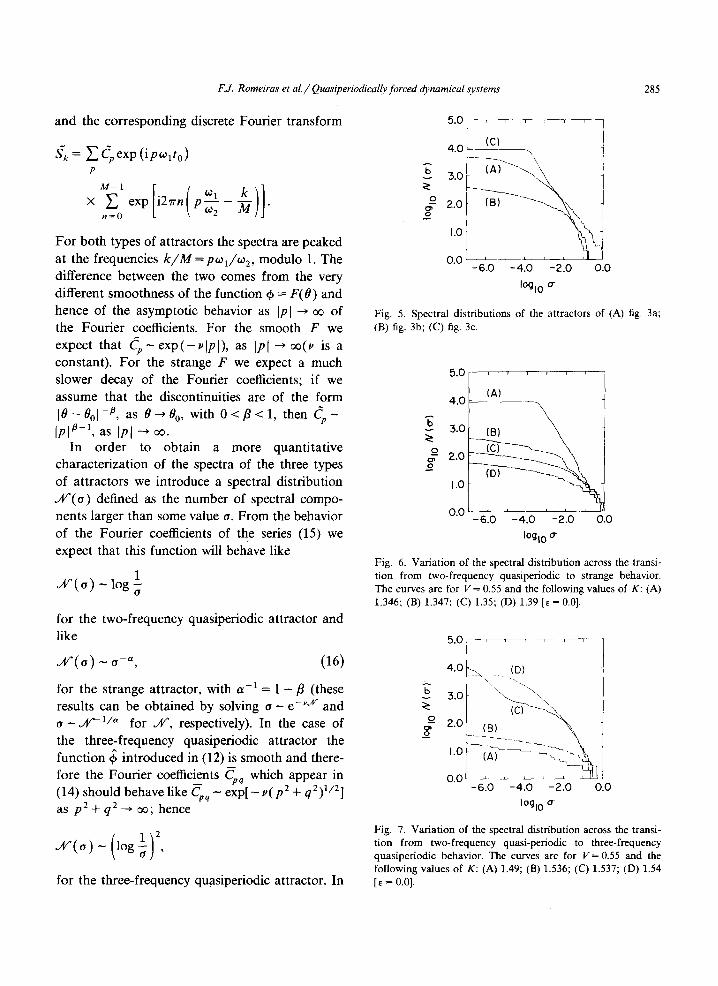
Fig. 5. Spectral distributions of the attractors of (A) fig. 3a; (B) fig. 3b; (C) fig. 3c.

0

o

5,0

4.0

3.0

2.0

1.0

0.0

r r i

(A)

(B) - - ~

'.0 . . . . . . -6 -4.0 -2.0 0.0 IOglo o

Fig. 6. Variation of the spectral distribution across the transition from two-frequency quasiperiodic to strange behavior. The curves are for V = 0.55 and the following values of K: (A) 1.346; (B) 1.347; (C) 1.35; (D) 1.39 [~ = 0.0].

i 4.O L (D)

3.o t " ~ ' \ \

-6.0 -4.0 -2.0 0.0 IOglo

Fig. 7. Variation of the spectral distribution across the transition from two-frequency quasi-periodic to three-frequency quasiperiodic behavior. The curves are for V= 0.55 and the following values of K: (A) 1.49; (B) 1.536; (C) 1.537; (D) 1.54 [~ = 0.0].

286

~ n 2~r

1.0

0.8

0.6

0.4

0.2

0-0.0

a

F.J. Romeiras et al./ Quasiperiodically forced dynamical systems

V=O.3

0.2 0.4 0.6 0.8 1.0 0.0 0.2 0.4 0.6

en b en 2"rr 2 n

V=0.4

0.8 1.0

~n 2"rr

0.6 ~ . . . . .

o.4 :i 0.2

- ' -0 .0 0.2 C

V=0.44

!. o.o o.a i.o

On

V--0.45 V=0.55

. . . . . . . . . . . . . . Ill . . . . . .

t . . . . . :i !

~ i,I

0.0 0.2 0.4 0.6 ).8 1.0 0.0 0.2 0.4 0.6 0.8 1.0

d en e an 2Tr 2Tr

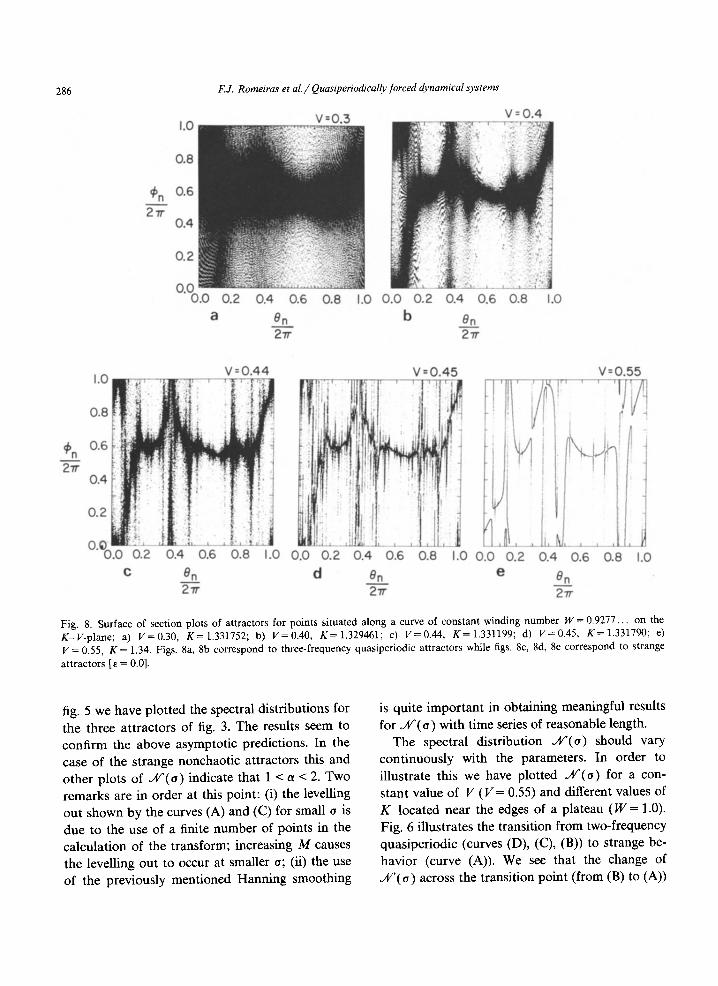
Fig. 8. Surface of section plots of attractors for points situated along a curve of constant winding number W = 0.9277... on the K-V-plane; a) V=0.30 , K=1.331752; b) V=0.40, K=1.329461; c) V=0.44, K=1.331199; d) V=0.45, K=1.331790; e) V = 0.55, K = 1.34. Figs. 8a, 8b correspond to three-frequency quasiperiodic attractors while figs. 8c, 8d, 8e correspond to strange

attractors [e = 0.0].

fig. 5 we have plotted the spectral distributions for the three attractors of fig. 3. The results seem to confirm the above asymptotic predictions. In the case of the strange nonchaotic attractors this and other plots of JV(O) indicate that 1 < a < 2. Two remarks are in order at this point: (i) the levelling out shown by the curves (A) and (C) for small o is due to the use of a finite number of points in the calculation of the transform; increasing M causes the levelling out to occur at smaller o; (ii) the use of the previously mentioned Hanning smoothing

is quite important in obtaining meaningful results for jlP(o) with time series of reasonable length.

The spectral distribution ~4/'(o) should vary continuously with the parameters. In order to illustrate this we have plotted ~AP(o) for a constant value of V (V = 0.55) and different values of K located near the edges of a plateau ( W = 1.0). Fig. 6 illustrates the transition from two-frequency quasiperiodic (curves (D), (C), (B)) to strange behavior (curve (A)). We see that the change of J4/'(o) across the transition point (from (B) to (A))


is much greater than the change of .A/'(o) for points on the plateau (for example (B) and (D)) even though the change from (B) to (A) corresponds to a much smaller variation in K (1 part in 1346 for the first case; 43 parts in 1347 for the second). Fig. 7 illustrates the transition from two- frequency quasiperiodic (curves (A), (B)) to three- frequency quasiperiodic behavior (curves (C), (D)). Again the change of ,Af(o) across the transition point (from (B) to (C)) is much greater and more rapid than the change corresponding to variations of K within the plateau (cf. figure caption for K values).

In order to illustrate the important transition from three-frequency quasiperiodic to strange behavior we have followed the evolution of the attractors along a curve of constant winding number in the KV-plane (the curve used, W = 0.9277 . . . . is plotted as curve (W) in fig. 1). As V is increased the three-frequency quasiperiodic attractor under- goes a transition to a strange attractor at some critical value V = V¢ (W). From the evidence of the numerical results (both the surface of section plots and the spectra) the transition seems to occur somewhere in the interval 0.42 < V < 0.44. [Note that the Lyapunov exponent does not help much in finding the transition very accurately as it is always very small over the interval 0.42 < V < 0.44 (IAI < 10-5).]

In figs. 8(a, b, c, d, e) we have plotted the surface of section plots of the attractors for several

0

5.0 , , , , , , ,

4 .0

5.0 i

2.0

1.0

0.0 -4J

(c) ~ . ,~(B)

(E) , (,E)',

-3 .0 - 2 . 0 - I . 0 0.0

Ioglo o" Fig. 9. Spectral distributions of the attractors of (A) fig. 3a; (B) fig. 3b; (C) fig. 3c; (E) fig. 3e.

pairs of (K, V) values along the constant winding number curve. In fig. 9 we have plotted the spectral distributions of some of these attractors. One point that is worth emphasizing is that the exponent introduced in eq. (16) has a value close to 2 near the transition point which then rapidly decreases to 1 as one moves away from this point. A heuristic argument for why ct approaches 1 is given in ref. 11.

3. The case e =/: 0

Eq. (2) with e = 0 is special in the sense that it is related to the linear Schr~Sdinger equation with quasiperiodic potential by Priifer's transformation. An interesting question to be asked is to what extent do equations of the more general form (4) exhibit behavior similar to that of eq. (2) with e = 0. In order to answer this question we have considered eq. (2) with e 4= 0. In all the numerical experiments reported here we have taken e = 0.2.

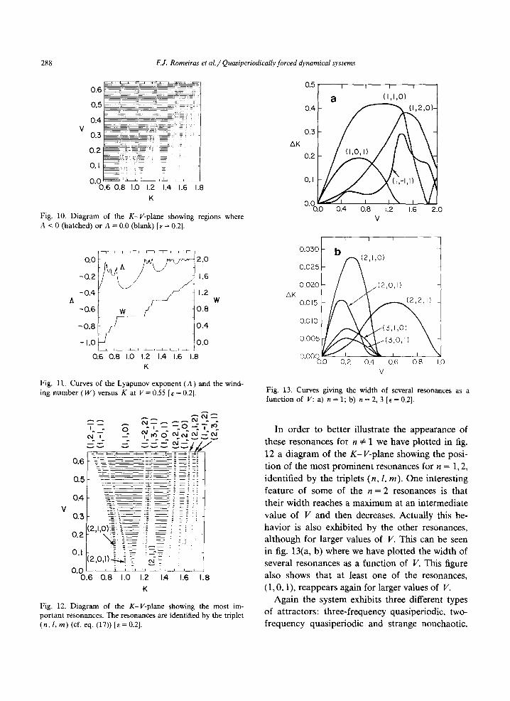
Fig. 10 shows a diagram of the KV-plane giving regions where A is negative (hatched) or zero (blank): the criterion for negative Lyapunov exponent is A < - 1 0 -4. Fig. 11 shows A and W versus K at a fixed value of V. The numerical procedure used to obtain these results for e = 0.2 is the same as used for the e -- 0 case, except that the grid in the K-V-plane was taken with 241 values of K.

These figures are qualitatively similar to those found in the case e = 0. An important difference is the more detailed structure corresponding to the appearance of a larger number of tongues and plateaus where the winding number is fixed. This is due to the fact that for e 4= 0 the plateaus occur at winding numbers

l m W = n~01 + -~--¢02, (17)

where l, m, and n are integers, whereas for e = 0 the plateaus occur at W = ho t + m~o 2, cf. eq. (11). This will be demonstrated analytically using perturbation theory in section 4.

288 F.J. Romeiras et al./ Quasiperiodically forced dynamical systems

V

0.6

0.5

0.4

0 . 5 - -

0.2

0.1

0.0 0.6 0.8 1.0

: : =

_--

1.2 1.4 1.6 1.8

Fig. 10. Diagram of the K-V-plane showing regions where A < 0 (hatched) or A = 0.0 (blank) [~ = 0.2].

0.0 , A

-0.2 ~ / J

-0.4 ~

'0.6 [ w o.a

-0.8 i / 0.4 - I . 0 . . . . . . 0.0

0.6 0.8 1.0 1.2 1.4 1.6 1.8 K

2.0

1.6

1.2 W

Fig. 11. Curves of the Lyapunov exponent (A) and the winding number (W) versus K at V= 0.55 [e = 0.2].

V

0A

0.5

0.2

0.1

0.0 - - ' 0.6

T - ~ - , - " - . o - . ' T r°

~5~ --": " N--',t/J

0.6 i 0.5

2 J , O ) i ~ i i ~ .- ~ . .

z,o,l 0.8 1.0 1.2 1.4 1.6 1.8

K

Fig. 12. Diagram of the K-V-plane showing the most important resonances. The resonances are identified by the triplet (n, 1, m) (cf. eq. (17)) [E = 0.2].

AK

0.5

0.4

0.3

0.2

0.1

0-00. 0

a (

0.4 0.8

I I I

(I,1,0)

,2,0)-

1.2 1.6 2.0 V

AK

o.o3o

0.025

0.020

o.o 15

o.o IO

0.005

o.ooo o.o

F U I I

b b ,1,o)

(2,o,I)

0.2 0.4 0.6 08 I o v

Fig. 13. Curves giving the width of several resonances as a function of V: a) n = 1; b) n = 2, 3 [e = 0.2].

In order to better illustrate the appearance of

these resonances for n #= 1 we have plotted in fig.

12 a d iagram of the K-V-p lane showing the posi- t ion of the most prominent resonances for n = 1, 2,

identified by the triplets (n, l, m), One interesting

feature of some of the n = 2 resonances is that

their width reaches a maximum at an intermediate

value of V and then decreases. Actually this behavior is also exhibited by the other resonances, a l though for larger values of V. This can be seen in fig. 13(a, b) where we have plotted the width of several resonances as a function of V. This figure also shows that at least one of the resonances,

(1, 0,1), reappears again for larger values of V. Again the system exhibits three different types

of at tractors: three-frequency quasiperiodic, two- f requency quasiperiodic and strange nonchaotic.

F.J. Romeiras et al. / Quasiperiodically forced dynamical systems 289

2rr

1.0

0.8

0.6 1 0.4

0.2

0.0 0.0 0.2 0.4 0.6 0.8 1.0

a On

I

, L

I ~ I J I _

0.0 0.2 0.4 0.6 0.8 1.0 0.0 0.2 0.4 0.6 0.8 1.0

b O n C O n 2Tr 27r

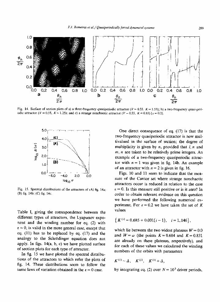
Fig. 14. Surface of section plots of a) a three-frequency quasiperiodic attractor ( V = 0.55. K = 1.53); b) a two-frequency quasi-periodic attractor ( V = 0.55, K = 1.25); and c) a strange nonchaotic attractor ( V = 0.55, K = 0.83) [e = 0.2].

L 4o~ to) d

3.0

I.o I )

0•0 -~ -6.0 -4.0 2.0 0.0

IOgl0 o"

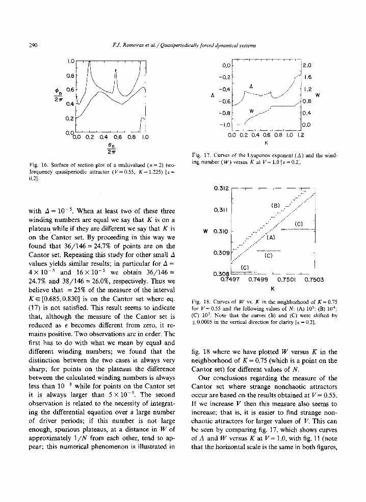
Fig. 15. Spectral distributions of the attractors of (A) fig. 14a; (B) fig. 14b; (C) fig. 14c.

Table I, giving the correspondence between the different types of attractors, the Lyapunov exponent and the winding number for eq. (2) with e = 0, is valid in the more general case, except that eq. (11) has to be replaced by eq. (17) and the analogy to the Schr'6dinger equation does not apply. In figs. 14(a, b, c) we have plotted surface of section plots for each type of attractor.

In fig. 15 we have plotted the spectral distributions of the attractors to which refer the plots of fig. 14. These distributions seem to follow the same laws of variation obtained in the e = 0 case.

One direct consequence of eq. (17) is that the two-frequency quasiperiodic attractor is now multivalued in the surface of section; the degree of multiplicity is given by n, provided that l, n and m, n are taken to be relatively prime integers• An example of a two-frequency quasiperiodic attractor with n = 1 was given in fig. 14b. An example of an attractor with n = 2 is given in fig. 16.

Figs. 10 and 11 seem to indicate that the measure of the Cantor set where strange nonchaotic attractors occur is reduced in relation to the case e = 0. Is this measure still positive or is it zero? In order to obtain relevant evidence on this question we have performed the following numerical ex- periment. For e---0.2 we have taken the set of K values

{ K ( ' ) = 0 . 6 8 5 + 0 . 0 0 1 ( i - 1 ) , i = 1 , 1 4 6 } ,

which lie between the two widest plateaus W = 0.0 and W = ~o (the points K = 0.684 and K = 0.831 are already on these plateaus, respectively), and for each of these values we calculated the winding numbers of the orbits with parameters

K ( i ) - A , K ( i ) , K(o + A,

by integrating eq. (2) over N = 105 driver periods,


0.8

Cn 0"600 ~ 0.4

0.2

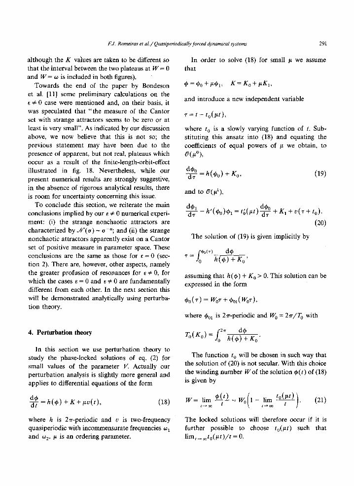
0 0.2 0.4 0.6 0.8 1.0 en 2"." Fig. 16. Surface of section plot of a multivalued (n = 2) two- frequency quasiperiodic attractor (V= 0.55, K= 1.225) [~ = 0.21.

with A = 10 -5. When at least two of these three

winding numbers are equal we say that K is on a

p la teau while if they are different we say that K is

on the Can to r set. By proceeding in this way we found that 36/146---24.7% of points are on the

Can to r set. Repeat ing this study for other small A

values yields similar results; in particular for A = 4 X 1 0 - 5 and 1 6 × 1 0 - 5 we obtain 3 6 / 1 4 6 =

24.7% and 38 /146 = 26.0%, respectively. Thus we

believe that --- 25% of the measure of the interval

K ~ [0.685,0.830] is on the Cantor set where eq.

(17) is not satisfied. This result seems to indicate

that, a l though the measure of the Cantor set is

reduced as e becomes different f rom zero, it remains positive. Two observations are in order. The

first has to do with what we mean by equal and

different winding numbers; we found that the

dist inct ion between the two cases is always very

sharp; for points on the plateaus the difference between the calculated winding numbers is always less than 10 8 while for points on the Cantor set

it is always larger than 5 × 10 -5. The second observat ion is related to the necessity of integrat-

ing the differential equation over a large number of driver periods; if this number is not large enough, spurious plateaus, at a distance in W of approximate ly 1 / N from each other, tend to appear; this numerical phenomenon is illustrated in

0.0

-0.2

-0.4

-0.6

-0.8

- I .0

/ ,

_4

/ /

w ~ j

f 0.0 0.2 0.4 0.6 0.8 I-.0 1.2

2.0

1.6

1.2

0.8

0.4

0.0

W

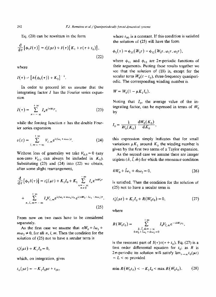
Fig. 17. Curves of the Lyapunov exponent (A) and the winding number (W) versus K at V= 1.0 [e = 0.2].

0.312

0.311

W 0.310

0.309

0.308 ....... T ........ ,

0.7497 0.7499

i i i I i

(B) .... ~- ++ , ,

. , , ' + +~ , , + *

,. ,-- (c) , , . ' " , . . ' + ++* . . . . . . . . . . . . . , . . . . .

,. ,..,'" (A)

" ' * * ~ . , ' ~ * ' ÷ . + , + * ÷ . + + H +* . . . .

,,"* (c)

(c) I t _ _ I _

0.7501 0,7505

K

Fig. 18. Curves of W vs. K in the neighborhood of K= 0.75 for V = 0.55 and the following values of N: (A) 105; (B) 104; (C) 103. Note that the curves (B) and (C) were shifted by + 0.0005 in the vertical direction for clarity [e = 0.2].

fig. 18 where we have plotted W versus K in the

ne ighborhood of K = 0.75 (which is a point on the

Can to r set) for different values of N. Our conclusions regarding the measure of the

Can to r set where strange nonchaot ic attractors occur are based on the results obtained at V = 0.55. If we increase V then this measure also seems to increase; that is, it is easier to find strange non-

chaot ic at tractors for larger values of V. This can be seen by compar ing fig. 17, which shows curves of A and W versus K at V = 1.0, with fig. 11 (note that the horizontal scale is the same in both figures,

F.J. Romeiras et aL / Quasiperiodically forced dynamical systems 291

although the K values are taken to be different so that the interval between the two plateaus at W = 0 and W = ~0 is included in both figures).

Towards the end of the paper by Bondeson et al. [11] some preliminary calculations on the e 4:0 case were mentioned and, on their basis, it was speculated that " the measure of the Cantor set with strange attractors seems to be zero or at least is very small". As indicated by our discussion above, we now believe that this is not so; the previous statement may have been due to the presence of apparent, but not real, plateaus which occur as a result of the finite-length-orbit-effect illustrated in fig. 18. Nevertheless, while our present numerical results are strongly suggestive, in the absence of rigorous analytical results, there is room for uncertainty concerning this issue.

To conclude this section, we reiterate the main conclusions implied by our e 4:0 numerical experi- ment: (i) the strange nonchaotic attractors are characterized by .# ' (o ) - o-a; and (ii) the strange nonchaotic attractors apparently exist on a Cantor set of positive measure in parameter space. These conclusions are the same as those for ~ = 0 (section 2). There are, however, other aspects, namely the greater profusion of resonances for e :# 0, for which the cases e = 0 and e 4:0 are fundamentally different from each other. In the next section this will be demonstrated analytically using perturba-

tion theory.

In order to solve (18) for small g we assume that

= ~0 + tL~bl, K = g o + gK1,

and introduce a new independent variable

1" = t - to (g t ),

where t o is a slowly varying function of t. Sub- stituting this ansatz into (18) and equating the coefficients of equal powers of g we obtain, to O(~°),

d,/,o d~" = h(q~°) + K° ' (19)

and to 0(~1),

dqhd'r h'(ePo)epl=to(gt)dd~ + K l + v ( ~ + t ° ) "

(20)

The solution of (19) is given implicitly by

f *o(,) d~ "o h ( ¢ ) + K o

assuming that h (¢ ) + K o > 0. This solution can be expressed in the form

= +

where q~Ol is 2¢r-periodic and W o = 2¢r/T o with

4. Perturbation theory

In this section we use perturbation theory to study the phase-locked solutions of eq. (2) for small values of the parameter V. Actually our perturbation analysis is slightly more general and applies to differential equations of the form

d4, d-7 = h( ep) + K + gv(t) , (18)

To( Ko) = fo2~, dep h(¢) + K o "

The function t o will be chosen in such way that the solution of (20) is not secular. With this choice the winding number W of the solution q,(t) of (18) is given by

W= lim e P ( t ) = w ° ( 1 - lim t°(~tt) ) t t-,o~ (21)

where h is 2~'-periodic and v is two-frequency quasiperiodic with incommensurate frequencies wl and ~2. /z is an ordering parameter.

The locked solutions will therefore occur if it is further possible to choose to(l~t ) such that lira t ~ ~to( gt ) / t = O.


Eq. (20) can be rewritten in the form

d d-~ [~l I ( ' r ) ] = tlo(~t) + I(~')[ K1 + v(~" + to)],

(22)

where

I(~') = [h(~o(~-)) + Ko1-1.

In order to proceed let us assume that the integrating factor I has the Fourier series expansion

+oo

I ( ~ ' ) = E I , ei"w°', (23)

where too is a constant. If this condition is satisfied the solution of (25) will have the form

01( ) = ¢11(Wo ) + ,o2,),

where q'n and qh2 are 2~r-periodic functions of their arguments. Putting these results together we see that the solution of (18) is, except for the secular term Wo( t - to) , three-frequency quasiperiodic. The corresponding winding number is

W = Wo(1 + IIKllo).

Noting that I o, the average value of the integrating factor, can be expressed in terms of W 0 by

while the forcing function v has the double Four- ier series expansion

I 0 = - - 1 dWo(Ko)

Wo( Ko) dKo

+o¢

v ( t ) = E Vl, m ei(lwl+m~°2)t (24) [, m ~ -- oo

Without loss of generality we take V0, o = 0 (any non-zero Vo, o can always be included in K0). Substituting (23) and (24) into (22) we obtain, after some slight rearrangement,

[thff(¢)] = tO(M) + K t I o + Kt E [n einW°~"

nn¢O °°

+ q-o¢ ~_, I V e i(l~l+m~°2)t° e i (nW°+l~x +mm2)~"

n l , m r t , [ , m ~ --o~

(25)

From now on two cases have to be considered separately.

As the first case we assume that nWo+ i~ 1 + m~02 :~ 0, for all n, 1, m. Then the condition for the solution of (25) not to have a secular term is

+ I q I o = o,

which, on integration, gives

this expression simply indicates that for small variations/~K 1 around K 0 the winding number is given by the first two terms of a Taylor expansion.

As the second case we assume there are integer triplets (h, f, th) for which the resonance condition

/~W0 '~ l ~ l d - / ~ o 9 2 ~-- 0 , (26)

is satisfied. Then the condition for the solution of (25) not to have a secular term is

t ; ( r - ) + KxIo + R(Woto) = o, (27)

where

R ( Woto ) = +oo Y'. I V~ e -i~w°t°

h l ,& h, [~ ,h= -o¢

hWo + lWl + tho:2=O

is the resonant part of I('r)v('r + to). Eq. (27) is a first order differential equation for to; as R is 2~'r-periodic its solution will satisfy l imt~ ooto(l~t) = L < oo provided

to(/~t) = -K l lo l~ t+ too , m i n R ( W o t o ) < - K l l o < m a x R ( W o t o ) , (28)


where L is such that 5. Conclusions

IoK 1 + R ( W o L ) = 0 .

From these results we conclude that in this second case (18) will have two-frequency quasiperiodic solutions with winding number W = W0, where W 0 satisfies (26), provided that the parameter K remains sufficiently close to K 0 so that (28) is satisfied. Note that condition (28) implies that the width (in K space) of the phase locked regions scales as the magnitude of R(Woto).

The perturbation results that we have just described are valid for (18) with arbitrary 2~r-periodic h and two-frequency quasiperiodic v. Let us now analyse the two special cases (i) h(~) = cos q~, for which (18) can be reduced to the SchrSdinger equation, and (ii) v(t) = K(cos O~zt + cos ~2t), as considered in the numerical work described in the present paper.

In case (i) it can be shown that the integrating factor for (20) has the form

= - 0 12 [r0 + sin (Wo +

where Wo(Ko) = (K~ - 1) 1/2 and cp is a constant. That is, I is monochromatic with frequency W 0. If we follow through the perturbation analysis we verify that in this special case the resonance condition (26) takes the form

Wo .-[-/"~ 1 q-/~/~2 = 0,

in agreement with our results of section 2. In case (ii), if we again follow through the

analysis, we verify that the resonance condition can only take one of the two particular forms

/~Wo--~-tOl ~--0 , / ~ W o - - [ - o ) 2 = 0 .

That is, to O(/xz), only resonances of one of these two forms can occur. Note, however, that resonances of the general form (26) can still be found in this case by taking the perturbation theory to ^ d~(#/+'~).

We have discussed the existence and properties of strange nonchaotic attractors exhibited by the first order ordinary differential equation with two-frequency quasiperiodic forcing, eq. (2). The following are the most important conclusions of our study:

i) For a fixed value of V the curve giving the winding number W as a function of K is a "devil's staircase": a continuous, non-decreasing curve with a dense set of open intervals on which the winding number is constant; between these intervals there is a Cantor set of apparently positive Lebesgue measure on which the winding number increases with K.

ii) On the intervals the Lyapunov exponent is always negative while on the Cantor set it is either negative (above the critical curve) or zero (below the critical curve).

iii) On the intervals the equation exhibits two- frequency quasi-periodic attractors. On the Cantor set the equation exhibits either three-frequency quasiperiodic attractors (when A = 0) or strange nonchaotic attractors (when A < 0).

iv) The frequency spectra of the three types of attractors have in general clearly distinctive characteristics. If we introduce a spectral distribution ,W'(o) giving the number of spectral components larger than some value a, then we have: ,/V(a) - o -~, 1 < a < 2, for strange nonchaotic attractors; ~ r ( o ) - l o g ( 1 / a ) , for two-frequency quasiperiodic attractors; ,AP(o) - log2(1 /o) , for three- frequency quasiperiodic attractors.

v) The equation we have studied can be considered as a strong damping model of the driven pendulum and Josephson junction. Our present results, namely those related to the form of the frequency spectrum of the attractors, indicate that it should be possible in experiments with these physical devices to identify the strange nonchaotic attractors via an ~ ( a ) diagnostic. This is even made more plausible by the fact that these attractors seem to exist on a set of positive measure.

Finally we note that the qualitative conclusions numerically obtained for eq. (2) are expected to

294 F.J. Romeiras et aL / Quasiperiodically forced dynamical systems

hold for general first order quasiperiodically forced equat ions of the form d c p / d t = gn(ep, t ) , where ~/

represents parameters and the explicit t depen-

dence of gn is quasiperiodic. In particular, our

results suggest that the existence of strange non-

chaot ic at tractors on a positive measure in param-

eter space should apply. [We emphasize, however,

that for e ~ 0 our evidence for the existence of

strange nonchao t ic attractors on a set of positive measure is purely numerical. A rigorous proof

confirming (or refuting) the numerical evidence

remains a challenging problem for future study.]

Acknowledgements

This work was supported by the U.S. Depar t - men t of Energy, Office of Basic Energy Sciences

(Appl ied Mathemat ics Program) and the Office of

Nava l Research. Filipe Romeiras was also sup-

por ted by the Portuguese Insti tuto Nacional de

I n v e s t i g a ~ o Cientifica during his sabbatical leave

f rom the Inst i tuto Superior Trcnico of the Uni- versidade Trcn ica de Lisboa.

References

[1] C. Grebogi, E. Ott, S. Pelikan and J.A. Yorke, Physica 13D (1984) 261.

[2] P. Grassberger, J. Stat. Phys. 26 (1981) 173. [3] J.P. Sethna and E.D. Siggia, Physica l lD (1984) 193. [4] K. Kaneko, Prog. Theor. Phys. 71 (1984) 282. [5] E.G. Gwinn and R.M. Westervelt, Phys. Rev. A 33 (1986)

4143. [6] R.L. Kautz and J.C. MacFarlane, Phys. Rev. A 33 (1986)

498. [7] F.J. Romeiras and E. Ott, Phys. Rev. A (1987) to be

published. [8] R. Johnson and J. Moser, Commun. Math. Phys. 84

(1982) 403. [9] B. Simon, Adv. Appl. Math. 3 (1982) 463.

[10] B. Souillard, Phys. Rep. 103 (1984) 41. [11] A. Bondeson, E. Ott and T.M. Antonsen Jr., Phys. Rev.

Lett. 55 (1985) 2103. [12] G. Benettin, L. Galgani, A. Giorgilli and J.-M. Strelcyn,

Meccanica 15 (1980) 21. [13] E.O. Brigham, The fast Fourier transform (Prentice-Hall,

Englewood Cliffs, NJ, 1974). [14] G.E. Powell and I.C. Percival, J. Phys. A: Math. Gen. 12

(1979) 2053. [15] W.P. Petersen, Commun. ACM 26 (1983) 1008. [16] R.L Devaney, An introduction to chaotic dynamical sys-

tems (Benjamin/Cummings, Menlo Park, CA, 1986). [17] S. Aubry and G. Andre, Ann. lsr. Phys. Soc. 3 (1980) 133. [18] C. Grebogi, E. Ott and J.A. Yorke, Physica 15D (1985)

354.

Documents

Quasiperiodically forced dynamical systems with strange nonchaotic attractors