Embed Size (px)
DESCRIPTION
Query Compilation. Evaluating Logical Query Plan Physical Query Plan. Source: our textbook, slides by Hector Garcia-Molina. Outline. Convert SQL query to a parse tree Semantic checking: attributes, relation names, types - PowerPoint PPT Presentation
Citation preview
1
Query Compilation
Evaluating Logical Query PlanPhysical Query Plan
Source: our textbook, slides by Hector Garcia-Molina
2
Outline Convert SQL query to a parse tree
Semantic checking: attributes, relation names, types Convert to a logical query plan (relational
algebra expression) deal with subqueries
Improve the logical query plan use algebraic transformations group together certain operators evaluate logical plan based on estimated size of
relations Convert to a physical query plan
search the space of physical plans choose order of operations complete the physical query plan
3
Estimating Sizes of Relations
Used in two places: to help decide between competing logical query
plans to help decide between competing physical
query plans
Notation review: T(R): number of tuples in relation R B(R): minimum number of block needed to store
R V(R,a): number of distinct values in R of
attribute a
4
Desiderata for Estimation Rules
1. Give accurate estimates2. Are easy (fast) to compute3. Are logically consistent: estimated size
should not depend on how the relation is computed
Here describe some simple heuristics.
All we really need is a scheme that properlyranks competing plans.
5
Estimating Size of Projection
This can be exactly computed Every tuple changes size by a
known amount.
6
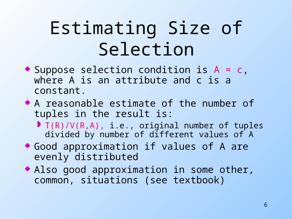
Estimating Size of Selection
Suppose selection condition is A = c, where A is an attribute and c is a constant.
A reasonable estimate of the number of tuples in the result is: T(R)/V(R,A), i.e., original number of tuples
divided by number of different values of A Good approximation if values of A are
evenly distributed Also good approximation in some other,
common, situations (see textbook)
7
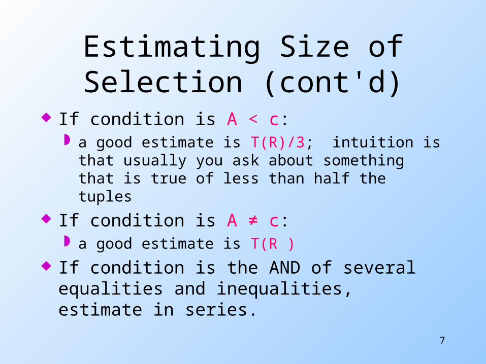
Estimating Size of Selection (cont'd)
If condition is A < c: a good estimate is T(R)/3; intuition is that
usually you ask about something that is true of less than half the tuples
If condition is A ≠ c: a good estimate is T(R )
If condition is the AND of several equalities and inequalities, estimate in series.
8
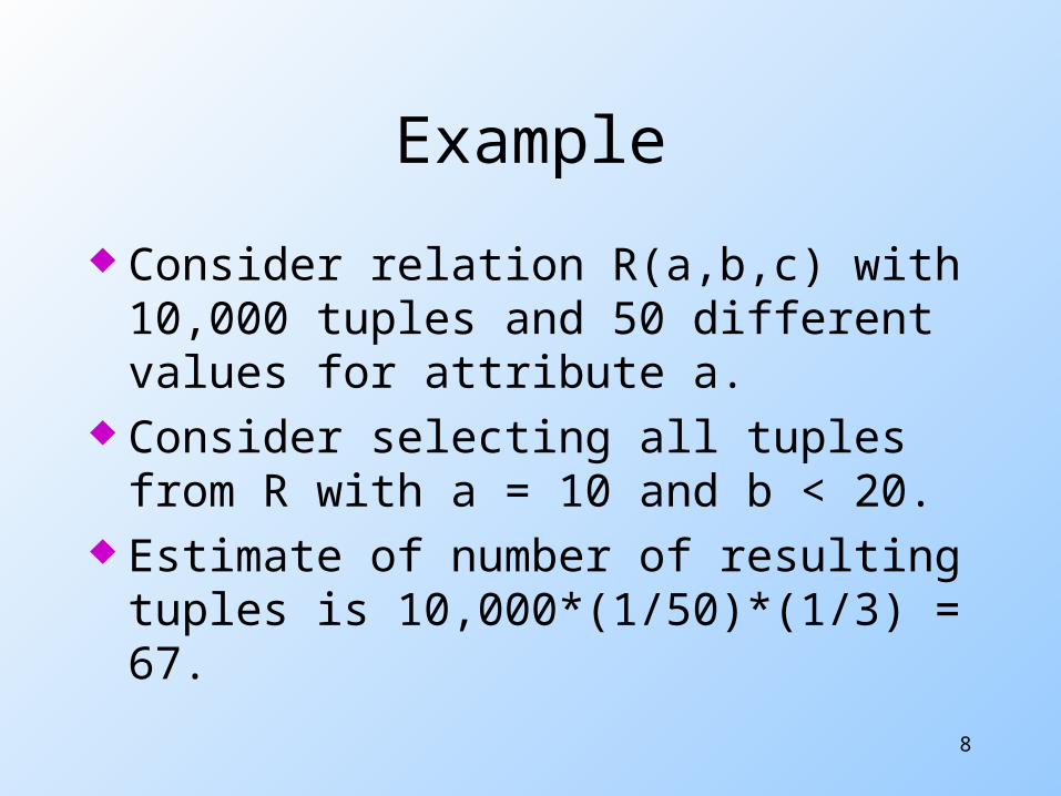
Example
Consider relation R(a,b,c) with 10,000 tuples and 50 different values for attribute a.
Consider selecting all tuples from R with a = 10 and b < 20.
Estimate of number of resulting tuples is 10,000*(1/50)*(1/3) = 67.
9
Estimating Size of Selection (cont'd)
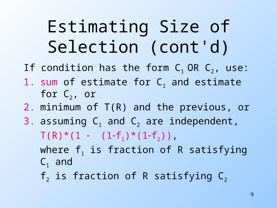
If condition has the form C1 OR C2, use:
1. sum of estimate for C1 and estimate for C2, or
2. minimum of T(R) and the previous, or3. assuming C1 and C2 are independent,
T(R)*(1 (1f1)*(1f2)),
where f1 is fraction of R satisfying C1 and
f2 is fraction of R satisfying C2
10
Example
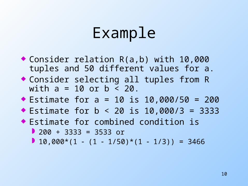
Consider relation R(a,b) with 10,000 tuples and 50 different values for a.
Consider selecting all tuples from R with a = 10 or b < 20.
Estimate for a = 10 is 10,000/50 = 200 Estimate for b < 20 is 10,000/3 = 3333 Estimate for combined condition is
200 + 3333 = 3533 or 10,000*(1 (1 1/50)*(1 1/3)) = 3466
11
Estimating Size of Natural Join
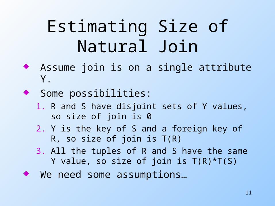
Assume join is on a single attribute Y. Some possibilities:
1. R and S have disjoint sets of Y values, so size of join is 0
2. Y is the key of S and a foreign key of R, so size of join is T(R)
3. All the tuples of R and S have the same Y value, so size of join is T(R)*T(S)
We need some assumptions…
12
Common Join Assumptions
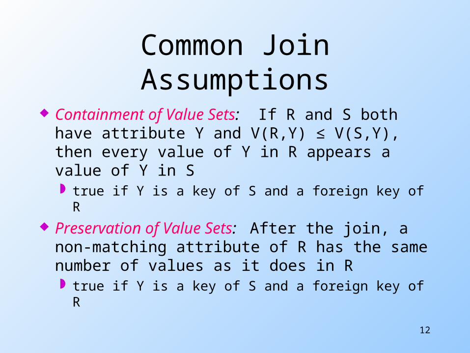
Containment of Value Sets: If R and S both have attribute Y and V(R,Y) ≤ V(S,Y), then every value of Y in R appears a value of Y in S true if Y is a key of S and a foreign key of R
Preservation of Value Sets: After the join, a non-matching attribute of R has the same number of values as it does in R true if Y is a key of S and a foreign key of R
13
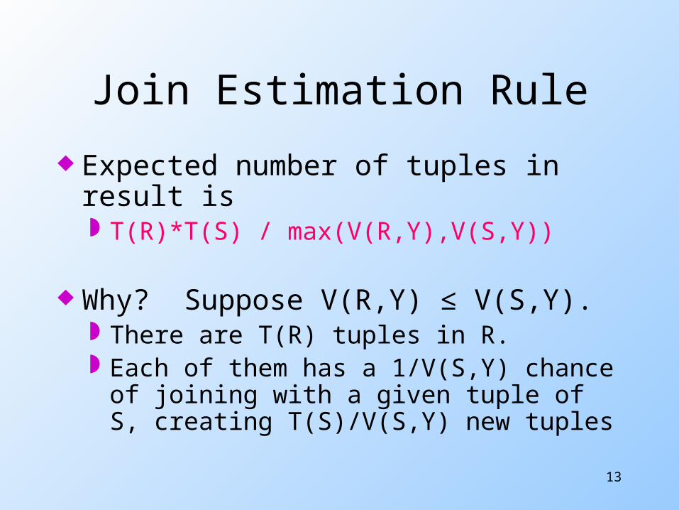
Join Estimation Rule
Expected number of tuples in result is T(R)*T(S) / max(V(R,Y),V(S,Y))
Why? Suppose V(R,Y) ≤ V(S,Y). There are T(R) tuples in R. Each of them has a 1/V(S,Y) chance of
joining with a given tuple of S, creating T(S)/V(S,Y) new tuples
14
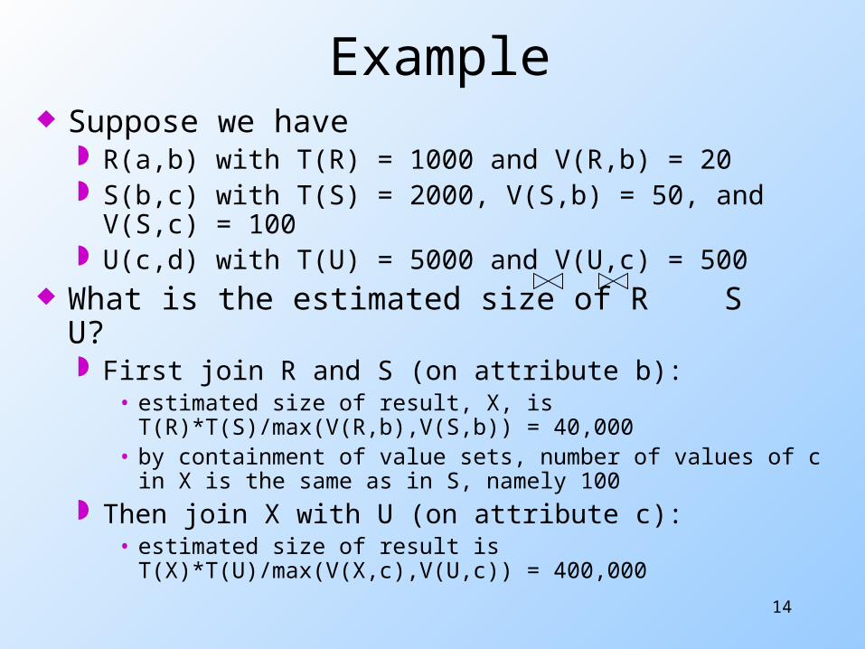
Example Suppose we have
R(a,b) with T(R) = 1000 and V(R,b) = 20 S(b,c) with T(S) = 2000, V(S,b) = 50, and V(S,c)
= 100 U(c,d) with T(U) = 5000 and V(U,c) = 500
What is the estimated size of R S U? First join R and S (on attribute b):
• estimated size of result, X, is T(R)*T(S)/max(V(R,b),V(S,b)) = 40,000
• by containment of value sets, number of values of c in X is the same as in S, namely 100
Then join X with U (on attribute c): • estimated size of result is T(X)*T(U)/max(V(X,c),V(U,c))
= 400,000
15
Example (cont'd)
If the joins are done in the opposite order, still get the same estimated answer
Due to preservation of value sets assumption.
This is desirable: we don't want the estimate to depend on how the result is computed
16
More About Natural Join If there are mutiple join attributes, the
previous rule generalizes: T(R)*T(S) divided by the larger of V(R,y)
and V(S,y) for each join attribute y
Consider the natural join of a series of relations: containment and preservation of value
sets assumptions ensure that the same estimated size is achieved no matter what order the joins are done in
17
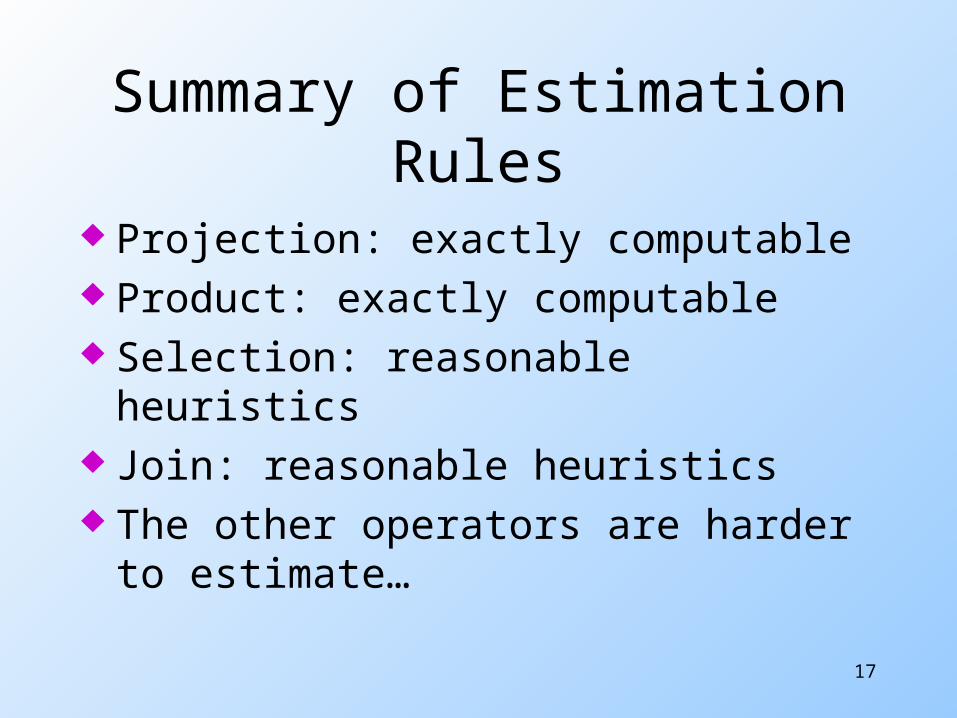
Summary of Estimation Rules
Projection: exactly computable Product: exactly computable Selection: reasonable heuristics Join: reasonable heuristics The other operators are harder to
estimate…
18
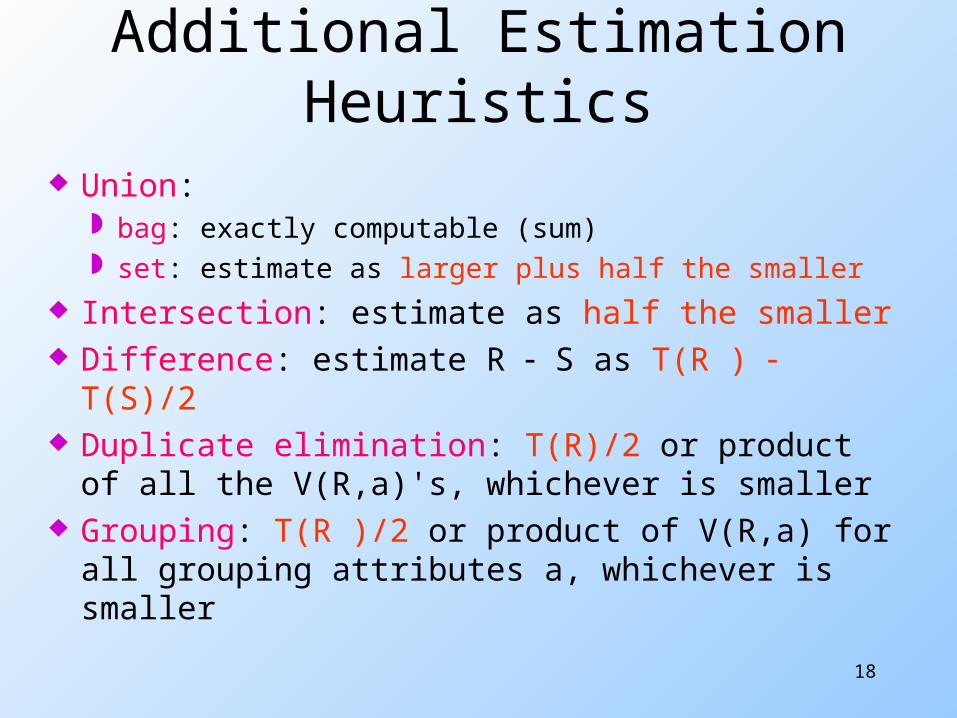
Additional Estimation Heuristics
Union: bag: exactly computable (sum) set: estimate as larger plus half the smaller
Intersection: estimate as half the smaller Difference: estimate R S as T(R ) T(S)/2 Duplicate elimination: T(R)/2 or product of
all the V(R,a)'s, whichever is smaller Grouping: T(R )/2 or product of V(R,a) for all
grouping attributes a, whichever is smaller
19
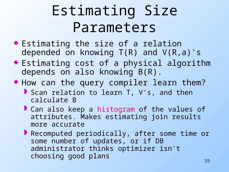
Estimating Size Parameters
Estimating the size of a relation depended on knowing T(R) and V(R,a)'s
Estimating cost of a physical algorithm depends on also knowing B(R).
How can the query compiler learn them? Scan relation to learn T, V's, and then calculate
B Can also keep a histogram of the values of
attributes. Makes estimating join results more accurate
Recomputed periodically, after some time or some number of updates, or if DB administrator thinks optimizer isn't choosing good plans
20
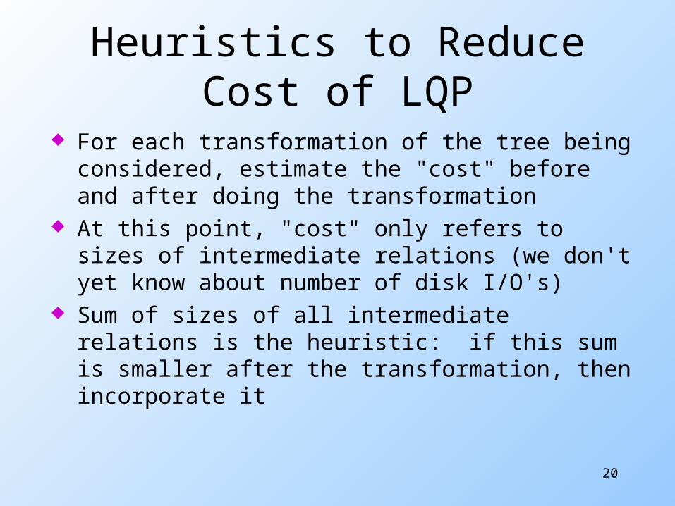
Heuristics to Reduce Cost of LQP
For each transformation of the tree being considered, estimate the "cost" before and after doing the transformation
At this point, "cost" only refers to sizes of intermediate relations (we don't yet know about number of disk I/O's)
Sum of sizes of all intermediate relations is the heuristic: if this sum is smaller after the transformation, then incorporate it
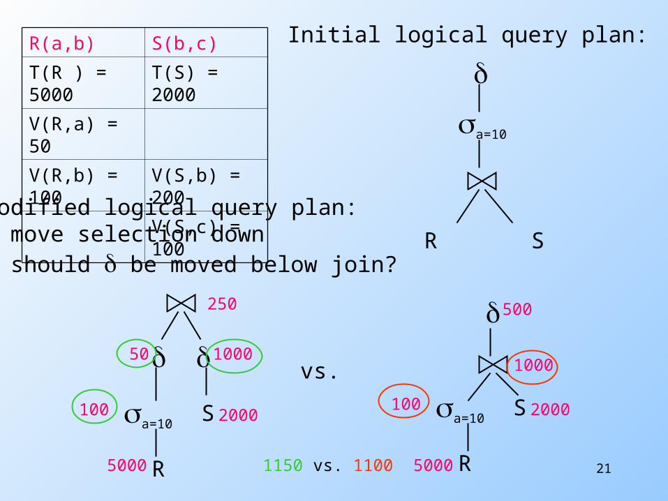
21
R(a,b) S(b,c)
T(R ) = 5000
T(S) = 2000
V(R,a) = 50
V(R,b) = 100
V(S,b) = 200
V(S,c) = 100
a=10
R S
Initial logical query plan:
Modified logical query plan:• move selection down• should be moved below join?
a=10 S
R
a=10
R
S
vs.
5000
2000 2000
5000
250
50 10001000
100 100
500
1150 vs. 1100
22
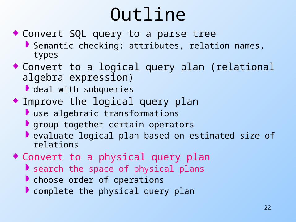
Outline Convert SQL query to a parse tree
Semantic checking: attributes, relation names, types Convert to a logical query plan (relational
algebra expression) deal with subqueries
Improve the logical query plan use algebraic transformations group together certain operators evaluate logical plan based on estimated size of
relations Convert to a physical query plan
search the space of physical plans choose order of operations complete the physical query plan
23
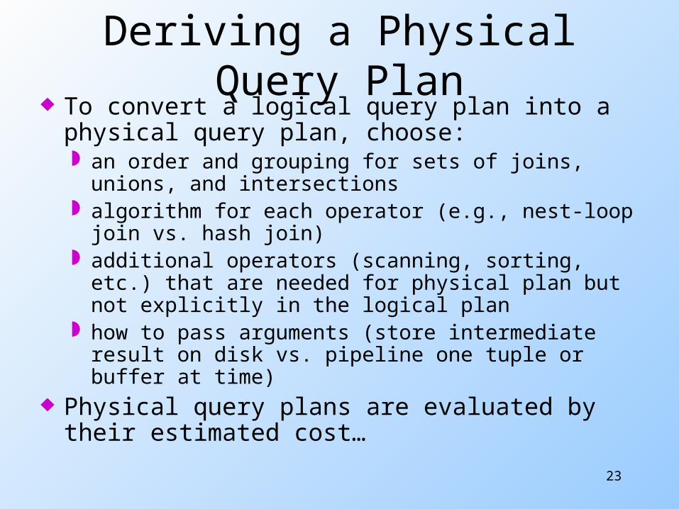
Deriving a Physical Query Plan
To convert a logical query plan into a physical query plan, choose: an order and grouping for sets of joins, unions,
and intersections algorithm for each operator (e.g., nest-loop join
vs. hash join) additional operators (scanning, sorting, etc.) that
are needed for physical plan but not explicitly in the logical plan
how to pass arguments (store intermediate result on disk vs. pipeline one tuple or buffer at time)
Physical query plans are evaluated by their estimated cost…
24
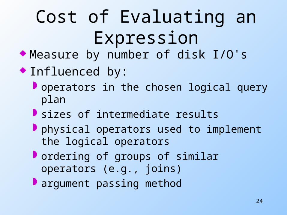
Cost of Evaluating an Expression
Measure by number of disk I/O's Influenced by:
operators in the chosen logical query plan sizes of intermediate results physical operators used to implement the
logical operators ordering of groups of similar operators
(e.g., joins) argument passing method
25
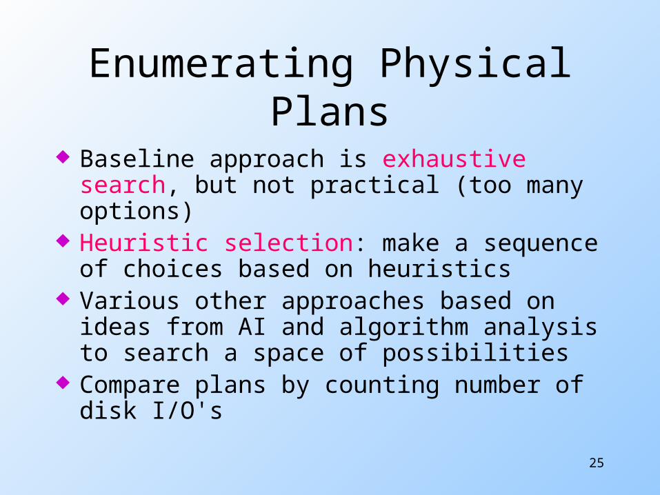
Enumerating Physical Plans
Baseline approach is exhaustive search, but not practical (too many options)
Heuristic selection: make a sequence of choices based on heuristics
Various other approaches based on ideas from AI and algorithm analysis to search a space of possibilities
Compare plans by counting number of disk I/O's
26
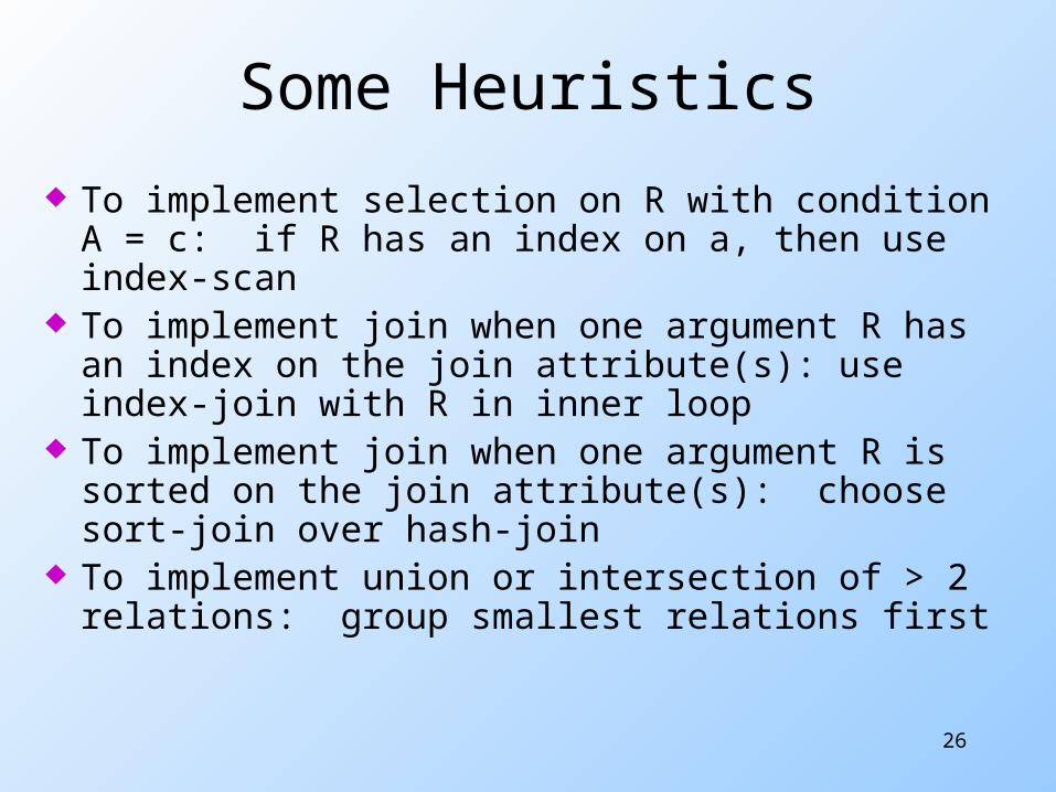
Some Heuristics
To implement selection on R with condition A = c: if R has an index on a, then use index-scan
To implement join when one argument R has an index on the join attribute(s): use index-join with R in inner loop
To implement join when one argument R is sorted on the join attribute(s): choose sort-join over hash-join
To implement union or intersection of > 2 relations: group smallest relations first
27
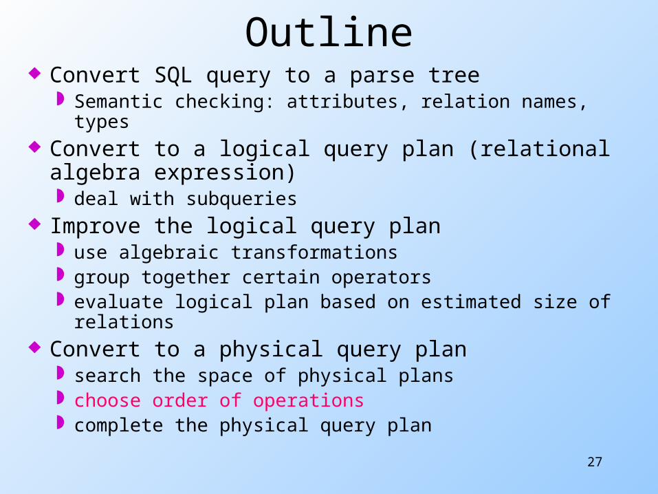
Outline Convert SQL query to a parse tree
Semantic checking: attributes, relation names, types Convert to a logical query plan (relational
algebra expression) deal with subqueries
Improve the logical query plan use algebraic transformations group together certain operators evaluate logical plan based on estimated size of
relations Convert to a physical query plan
search the space of physical plans choose order of operations complete the physical query plan
28
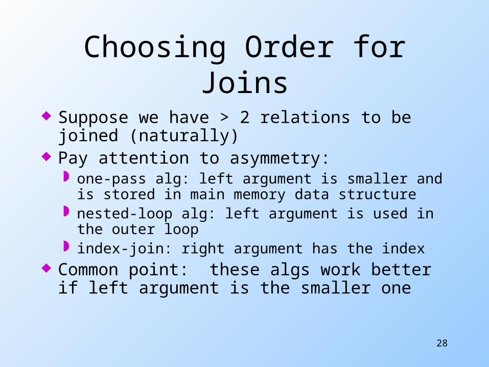
Choosing Order for Joins
Suppose we have > 2 relations to be joined (naturally)
Pay attention to asymmetry: one-pass alg: left argument is smaller and is
stored in main memory data structure nested-loop alg: left argument is used in the
outer loop index-join: right argument has the index
Common point: these algs work better if left argument is the smaller one
29
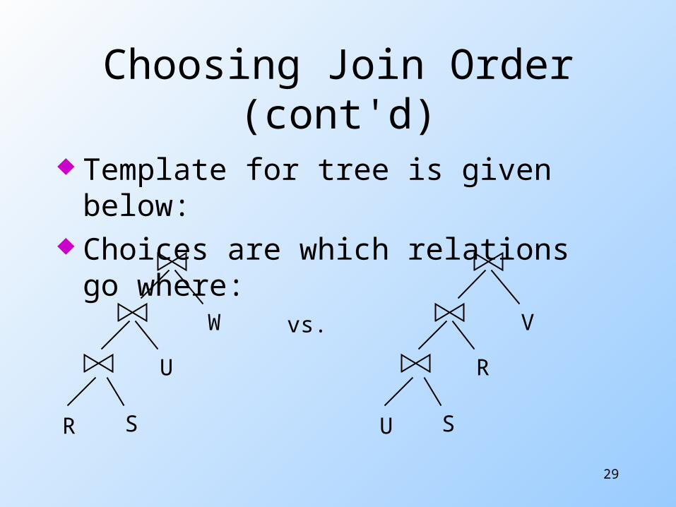
Choosing Join Order (cont'd)
Template for tree is given below: Choices are which relations go
where:
R S
U
W
U S
R
Vvs.
30
Choosing Join Order (cont'd)
How do we decide on the leaves? Try all possibilities. Not a good idea:
there are n! choices, where n is the number of relations to be joined
Use dynamic programming, a technique from analysis of algorithms. Works well for relatively small values of n
Heuristic approach with a greedy algorithm, works faster but doesn't always find the best ordering
31
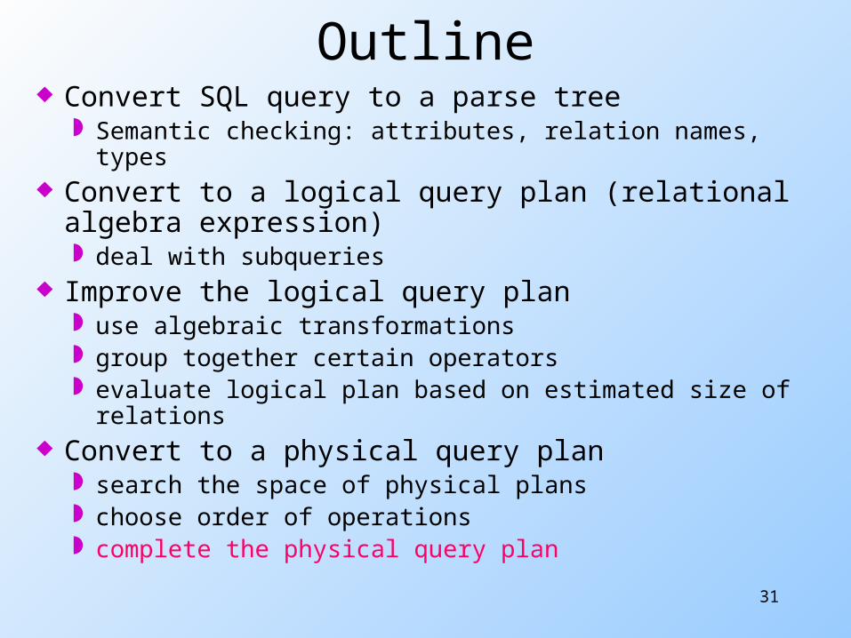
Outline Convert SQL query to a parse tree
Semantic checking: attributes, relation names, types Convert to a logical query plan (relational
algebra expression) deal with subqueries
Improve the logical query plan use algebraic transformations group together certain operators evaluate logical plan based on estimated size of
relations Convert to a physical query plan
search the space of physical plans choose order of operations complete the physical query plan
32
Remaining Steps
Choose algorithms for remaining operators
Decide when intermediate results will be materialized (stored on disk in entirety) or pipelined (created only in main memory, in pieces)
33
Choosing Selection Method
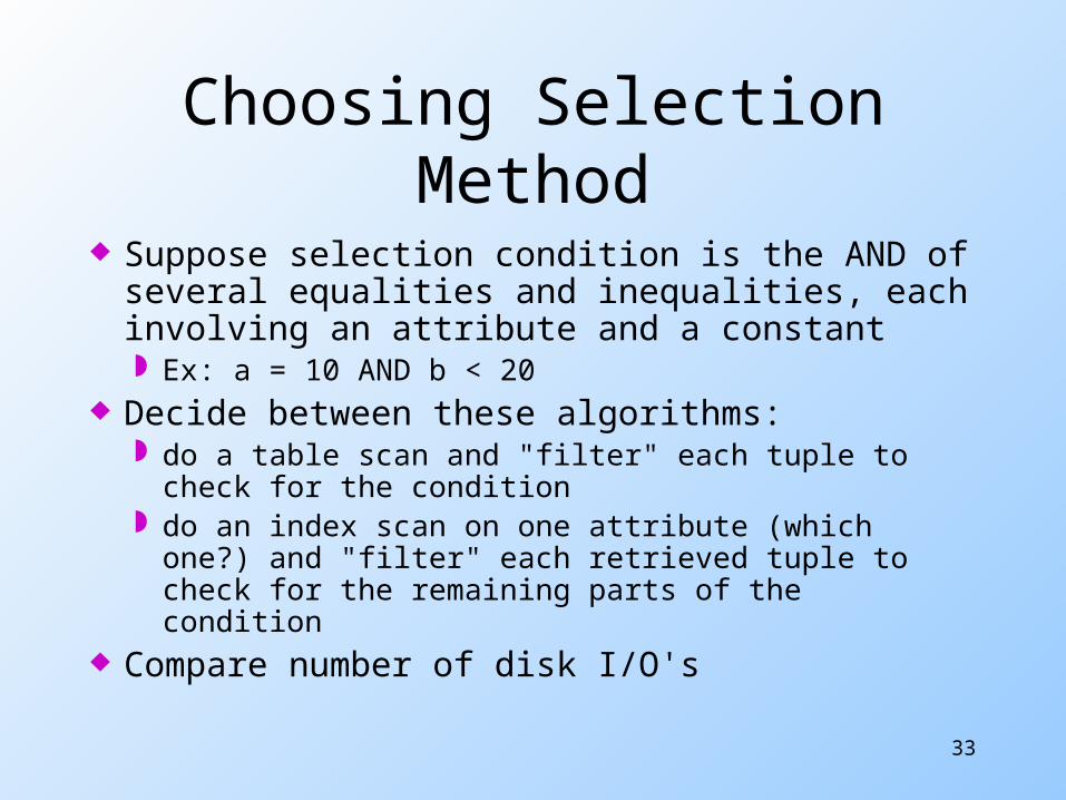
Suppose selection condition is the AND of several equalities and inequalities, each involving an attribute and a constant Ex: a = 10 AND b < 20
Decide between these algorithms: do a table scan and "filter" each tuple to check
for the condition do an index scan on one attribute (which one?)
and "filter" each retrieved tuple to check for the remaining parts of the condition
Compare number of disk I/O's
34
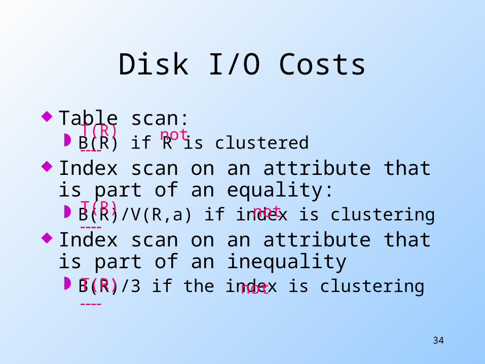
Disk I/O Costs
Table scan: B(R) if R is clustered
Index scan on an attribute that is part of an equality: B(R)/V(R,a) if index is clustering
Index scan on an attribute that is part of an inequality B(R)/3 if the index is clustering
T(R)
T(R)
T(R)
not
not
not
35
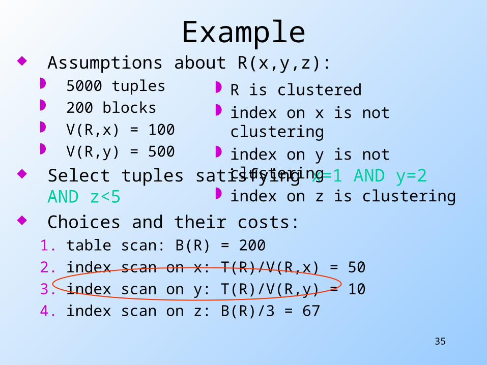
Example Assumptions about R(x,y,z):
5000 tuples 200 blocks V(R,x) = 100 V(R,y) = 500
Select tuples satisfying x=1 AND y=2 AND z<5
Choices and their costs:1. table scan: B(R) = 2002. index scan on x: T(R)/V(R,x) = 503. index scan on y: T(R)/V(R,y) = 104. index scan on z: B(R)/3 = 67
R is clustered index on x is not clustering index on y is not clustering index on z is clustering
36
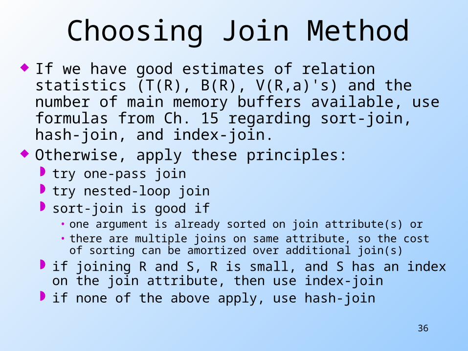
Choosing Join Method If we have good estimates of relation statistics
(T(R), B(R), V(R,a)'s) and the number of main memory buffers available, use formulas from Ch. 15 regarding sort-join, hash-join, and index-join.
Otherwise, apply these principles: try one-pass join try nested-loop join sort-join is good if
• one argument is already sorted on join attribute(s) or• there are multiple joins on same attribute, so the cost of
sorting can be amortized over additional join(s) if joining R and S, R is small, and S has an index on
the join attribute, then use index-join if none of the above apply, use hash-join
37
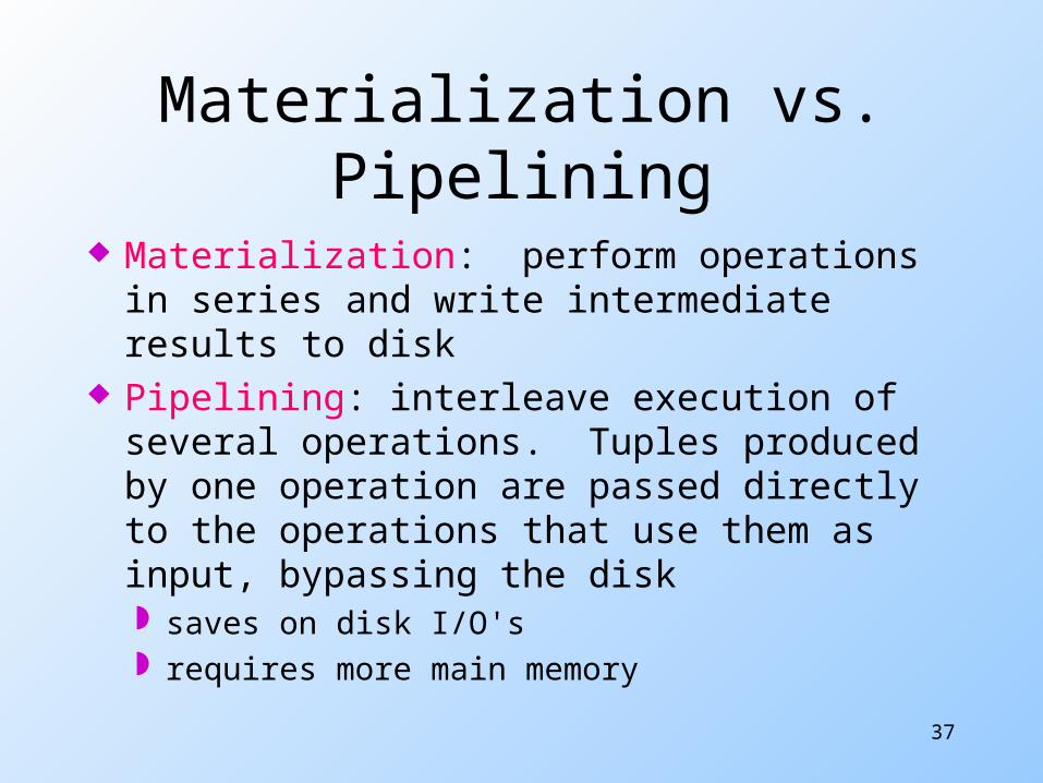
Materialization vs. Pipelining
Materialization: perform operations in series and write intermediate results to disk
Pipelining: interleave execution of several operations. Tuples produced by one operation are passed directly to the operations that use them as input, bypassing the disk saves on disk I/O's requires more main memory
38
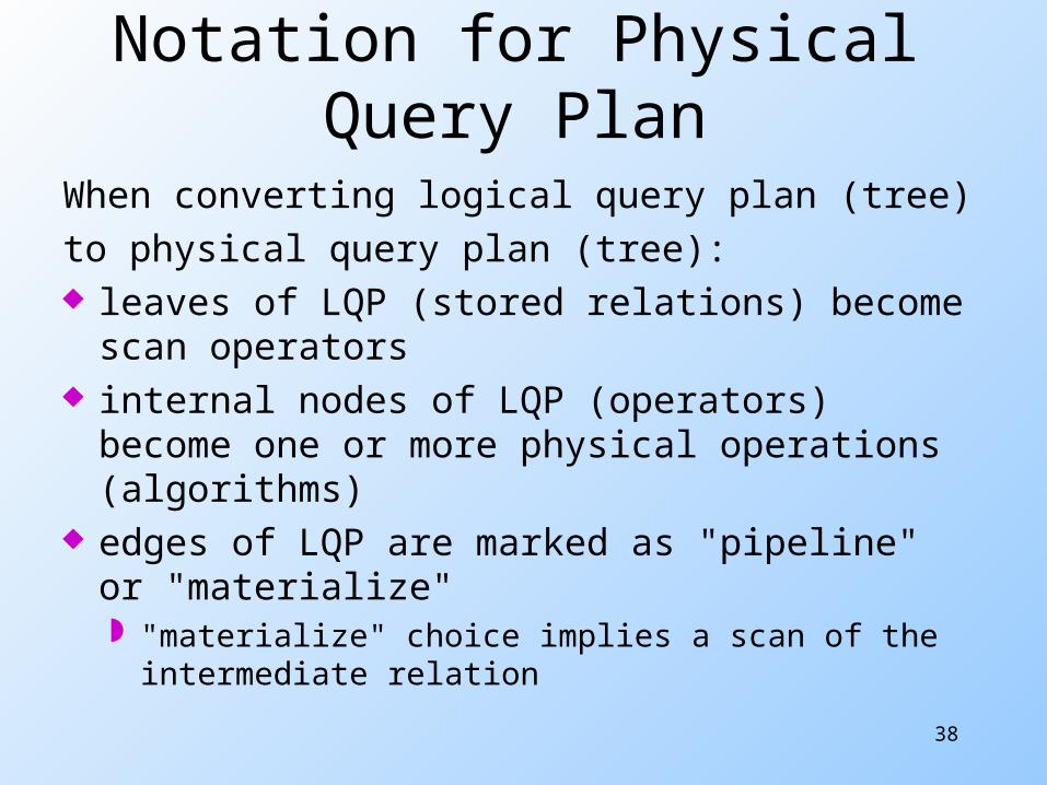
Notation for Physical Query Plan
When converting logical query plan (tree)to physical query plan (tree): leaves of LQP (stored relations) become
scan operators internal nodes of LQP (operators) become
one or more physical operations (algorithms)
edges of LQP are marked as "pipeline" or "materialize" "materialize" choice implies a scan of the
intermediate relation
39
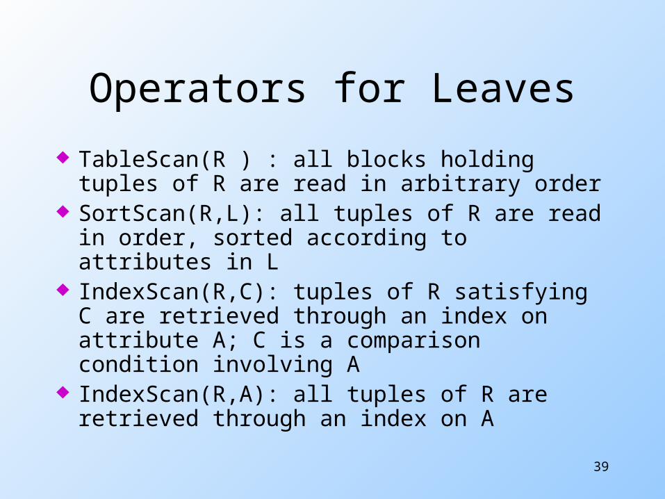
Operators for Leaves
TableScan(R ) : all blocks holding tuples of R are read in arbitrary order
SortScan(R,L): all tuples of R are read in order, sorted according to attributes in L
IndexScan(R,C): tuples of R satisfying C are retrieved through an index on attribute A; C is a comparison condition involving A
IndexScan(R,A): all tuples of R are retrieved through an index on A
40
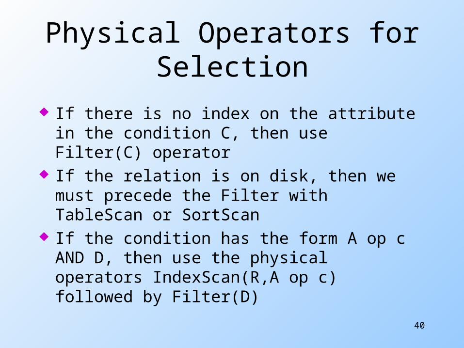
Physical Operators for Selection
If there is no index on the attribute in the condition C, then use Filter(C) operator
If the relation is on disk, then we must precede the Filter with TableScan or SortScan
If the condition has the form A op c AND D, then use the physical operators IndexScan(R,A op c) followed by Filter(D)
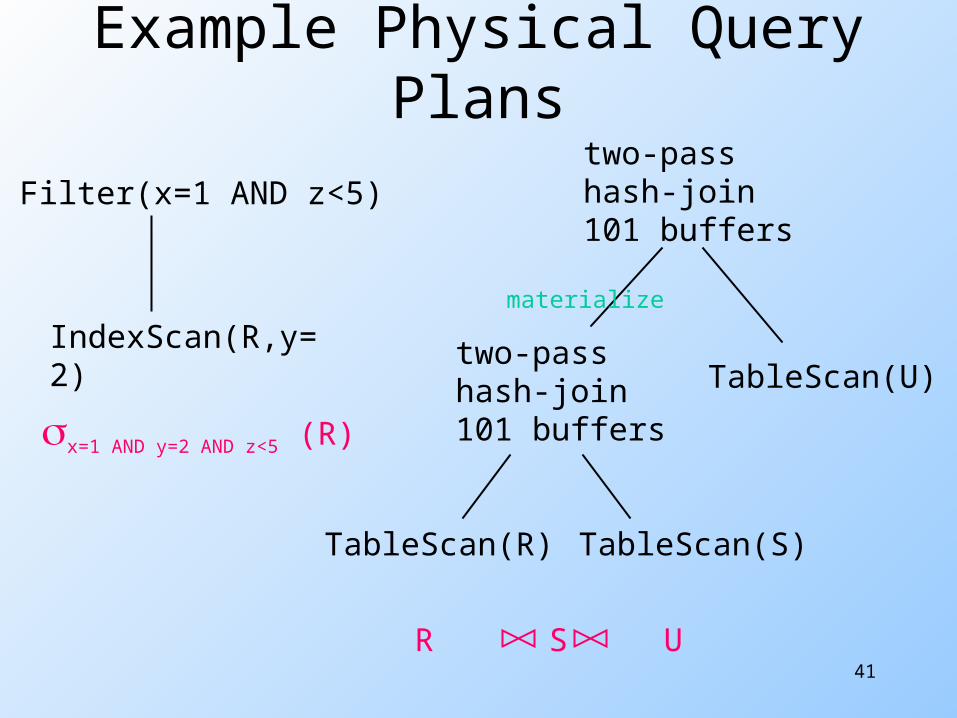
41
Example Physical Query Plans
Filter(x=1 AND z<5)
IndexScan(R,y=2)
two-passhash-join101 buffers
two-passhash-join101 buffers
TableScan(U)
TableScan(R) TableScan(S)
materialize
R S U
x=1 AND y=2 AND z<5 (R)


![Cypher: An Evolving Query Language for Property Graphs query planning in Neo4j is based on the IDP algorithm [44, 54], using a cost model described in [21]. The final query compilation](https://img.pdfslide.net/doc/110x75/5b4035527f8b9a4b3f8d0f4b/cypher-an-evolving-query-language-for-property-graphs-query-planning-in-neo4j-is.jpg)


![Welcome [tc18.tableau.com] · 2020-01-06 · Hyper compiles each SQL query to machine code and then executes this code. Traditional Interpretation vs. Compilation Traditional Interpreting](https://img.pdfslide.net/doc/110x75/5ed5ffe31e7606671009b0cf/welcome-tc18-2020-01-06-hyper-compiles-each-sql-query-to-machine-code-and.jpg)