Query Optimization II

R&G, Chapters 12, 13, 14Lecture 9

Administrivia

• Homeworks 2 and 3 have been switched around.

• The new Hw2 will be due in ~2 weeks.

• Midterm in ~3 weeks.

Review – the Big Picture

• Data Modelling– Relational– E-R

• Storing Data– File Indexes– Buffer Pool Management

• Query Languages– SQL– Relational Algebra– Relational Calculus– Formal Query Languages permit Query Optimization

Review – Query Optimization 1

• External Sorting with Merge sort– It is possible to sort most tables in 2 passes

• Join Algorithms– Nested Loops– Indexed Nested Loops– Sort-Merge Join– Hash Join

Review – Cost of Join Methods

• Blocked Nested LoopsM + M / B * N

• Indexed Nested LoopsM + ( (M*pR) * cost to find matching tuples)

• Sort-Merge Joinbetween 3(M+N) and M*N

• Hash Join3(M+N) and higher, especially with skewed

data

Today: Finding a Better Query

• Query Languages based on formal foundation

• Just as regular algebra expressions can be rewritten, so can relational algebra:

A*B = B*A, A(B + C) = AB + AC, etc.

AB = BC, etc.

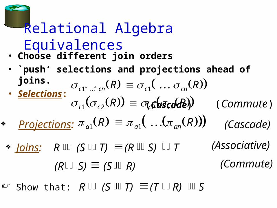
Relational Algebra Equivalences• Choose different join orders• `push’ selections and projections ahead of joins.• Selections:

(Cascade) c cn c cnR R1 1 ... . . .

c c c cR R1 2 2 1 (Commute)

Projections: a a anR R1 1 . . . (Cascade)

Joins: R (S T) (R S) T (Associative)

(R S) (S R) (Commute)

R (S T) (T R) S Show that:

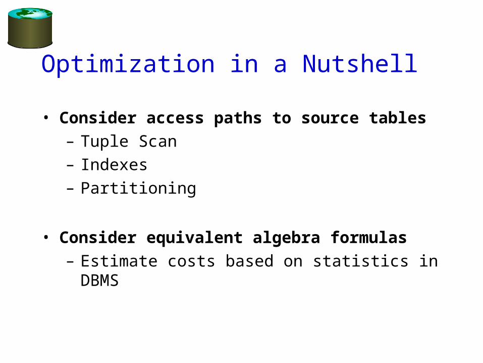
Optimization in a Nutshell

• Consider access paths to source tables– Tuple Scan– Indexes– Partitioning

• Consider equivalent algebra formulas– Estimate costs based on statistics in DBMS

Or, in more detail...• Plan: Tree of R.A. ops, with choice of alg for each

op.– Each operator typically implemented using a `pull’

interface: when an operator is `pulled’ for the next output tuples, it `pulls’ on its inputs and computes them.

• Two main issues:– For a given query, what plans are considered?

• Algorithm to search plan space for cheapest (estimated) plan.

– How is the cost of a plan estimated?• Ideally: Want to find best plan. • Practically: Avoid worst plans!• We will study the System R approach.

Schema for Examples

• Similar to old schema; rname added for variations.• Reserves:

– Each tuple is 40 bytes long, – 100 tuples per page, – M = 1000 pages total.

• Sailors:– Each tuple is 50 bytes long, – 80 tuples per page, – N = 500 pages total.

Sailors (sid: integer, sname: string, rating: integer, age: real)Reserves (sid: integer, bid: integer, day: dates, rname: string)

Statistics and Catalogs• Need information about the relations and indexes

involved. Catalogs typically contain at least:– # tuples (NTuples), # pages (NPages) for each relation.– # distinct key values (NKeys) and NPages for each index.– Index height, low/high key values (Low/High) for each

tree index.

• Catalogs updated periodically.– Updating whenever data changes is too expensive; lots

of approximation anyway, so slight inconsistency ok.

• More detailed information sometimes stored.– e.g., histograms of the values in some fields

Access Paths An access path is a method of retrieving

tuples: File scan, or index that matches a selection (in

the query) A tree index matches (a conjunction of)

terms that involve only attributes in a prefix of the search key. E.g., Tree index on <a, b, c> matches the

selection a=5 AND b=3, and a=5 AND b>6, but not b=3.

A hash index matches (a conjunction of) terms that has a term attribute = value for every attribute in the search key of the index. E.g., Hash index on <a, b, c> matches a=5 AND

b=3 AND c=5; but it does not match b=3, or a=5 AND b=3, or a>5 AND b=3 AND c=5.

A Note on Complex Selections

• Selection conditions are first converted to conjunctive normal form (CNF):

(day<8/9/94 OR bid=5 OR sid=3 ) AND (rname=‘Paul’ OR bid=5 OR sid=3)

• We only discuss case with no ORs; see text if you are curious about the general case.

(day<8/9/94 AND rname=‘Paul’) OR bid=5 OR sid=3

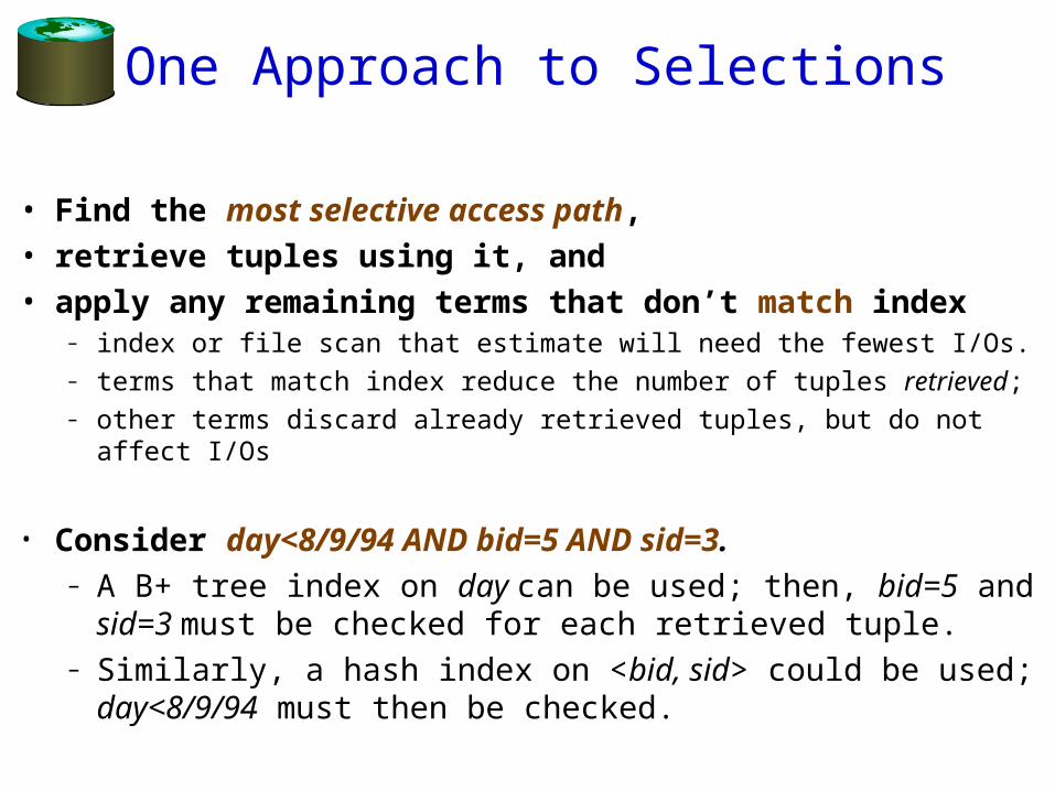
One Approach to Selections

• Find the most selective access path, • retrieve tuples using it, and • apply any remaining terms that don’t match index

– index or file scan that estimate will need the fewest I/Os.– terms that match index reduce the number of tuples retrieved; – other terms discard already retrieved tuples, but do not affect

I/Os

• Consider day<8/9/94 AND bid=5 AND sid=3. – A B+ tree index on day can be used; then, bid=5 and

sid=3 must be checked for each retrieved tuple. – Similarly, a hash index on <bid, sid> could be used;

day<8/9/94 must then be checked.

Using an Index for Selections

• Cost depends on #qualifying tuples, and clustering.– Cost of finding qualifying data entries (typically

small) plus cost of retrieving records (could be large w/o clustering).

– In example, assuming uniform distribution of names, about 10% of tuples qualify (100 pages, 10000 tuples). With a clustered index, cost is little more than 100 I/Os; if unclustered, upto 10000 I/Os!

SELECT *FROM Reserves RWHERE R.rname < ‘C%’

Projection

• The expensive part is removing duplicates.– SQL systems don’t remove duplicates unless the

DISTINCT is specified.

• Sorting Approach: Sort on <sid, bid> and remove duplicates. (Can optimize by dropping unwanted information while sorting.)

• Hashing Approach: Hash on <sid, bid> to create partitions. Load partitions into memory one at a time, build in-memory hash structure, and eliminate duplicates.

• If there is an index with both R.sid and R.bid in the search key, may be cheaper to sort data entries!

SELECT DISTINCT R.sid, R.bidFROM Reserves R

Join: Index Nested Loops

• If there is an index on the join column of one relation (say S), can make it the inner and exploit the index.– Cost: M + ( (M*pR) * cost of finding matching S tuples)

• For each R tuple, cost of probing S index is about 1.2 for hash index, 2-4 for B+ tree. Cost of then finding S tuples (assuming Alt. (2) or (3) for data entries) depends on clustering.– Clustered index: 1 I/O (typical), unclustered: up to 1

I/O per matching S tuple.

foreach tuple r in R doforeach tuple s in S where ri == sj do

add <r, s> to result

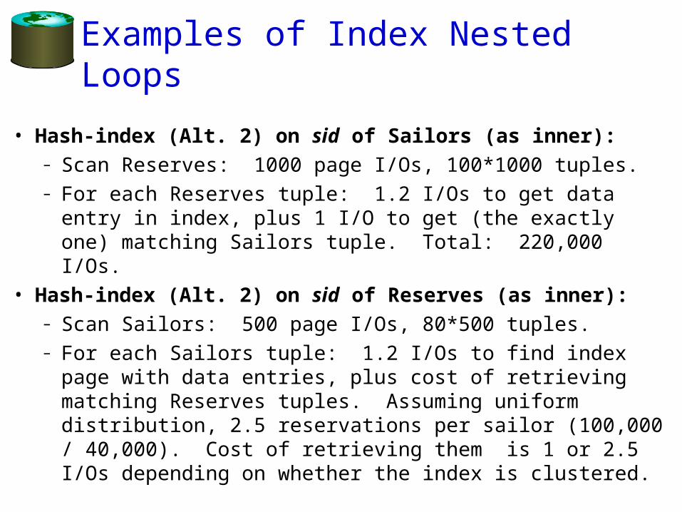
Examples of Index Nested Loops

• Hash-index (Alt. 2) on sid of Sailors (as inner):– Scan Reserves: 1000 page I/Os, 100*1000 tuples.– For each Reserves tuple: 1.2 I/Os to get data entry in

index, plus 1 I/O to get (the exactly one) matching Sailors tuple. Total: 220,000 I/Os.

• Hash-index (Alt. 2) on sid of Reserves (as inner):– Scan Sailors: 500 page I/Os, 80*500 tuples.– For each Sailors tuple: 1.2 I/Os to find index page

with data entries, plus cost of retrieving matching Reserves tuples. Assuming uniform distribution, 2.5 reservations per sailor (100,000 / 40,000). Cost of retrieving them is 1 or 2.5 I/Os depending on whether the index is clustered.

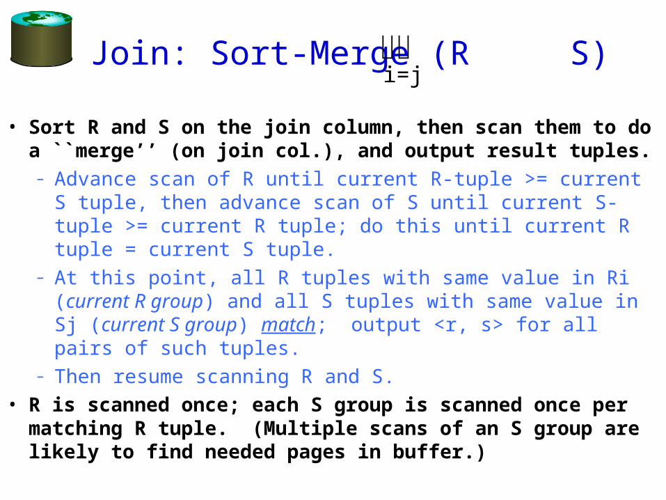
Join: Sort-Merge (R S)

• Sort R and S on the join column, then scan them to do a ``merge’’ (on join col.), and output result tuples.– Advance scan of R until current R-tuple >= current S

tuple, then advance scan of S until current S-tuple >= current R tuple; do this until current R tuple = current S tuple.

– At this point, all R tuples with same value in Ri (current R group) and all S tuples with same value in Sj (current S group) match; output <r, s> for all pairs of such tuples.

– Then resume scanning R and S.• R is scanned once; each S group is scanned once per

matching R tuple. (Multiple scans of an S group are likely to find needed pages in buffer.)

i=j

Example of Sort-Merge Join

• Cost: M log M + N log N + (M+N)– The cost of scanning, M+N, could be M*N (very unlikely!)

• With 35, 100 or 300 buffer pages, both Reserves and Sailors can be sorted in 2 passes; total join cost: 7500.

sid sname rating age22 dustin 7 45.028 yuppy 9 35.031 lubber 8 55.544 guppy 5 35.058 rusty 10 35.0

sid bid day rname

28 103 12/4/96 guppy28 103 11/3/96 yuppy31 101 10/10/96 dustin31 102 10/12/96 lubber31 101 10/11/96 lubber58 103 11/12/96 dustin

Highlights of System R Optimizer

• Impact:– Most widely used currently; works well for < 10 joins.

• Cost estimation: Approximate art at best.– Statistics, maintained in system catalogs, used to

estimate cost of operations and result sizes.– Considers combination of CPU and I/O costs.

• Plan Space: Too large, must be pruned.– Only the space of left-deep plans is considered.

• Left-deep plans allow output of each operator to be pipelined into the next operator without storing it in a temporary relation.

– Cartesian products avoided.

Cost Estimation

• For each plan considered, must estimate cost:– Must estimate cost of each operation in

plan tree.• Depends on input cardinalities.• We’ve already discussed how to estimate the

cost of operations (sequential scan, index scan, joins, etc.)

– Must also estimate size of result for each operation in tree!

• Use information about the input relations.• For selections and joins, assume independence of

predicates.

Size Estimation and Reduction Factors

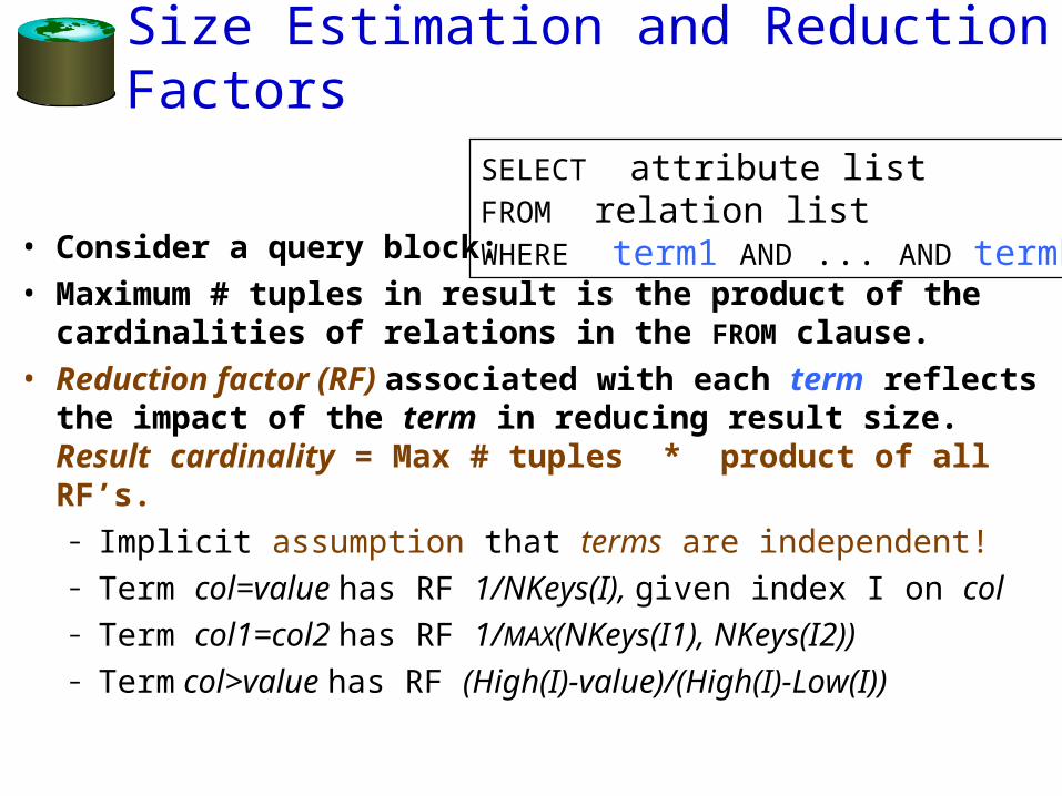
• Consider a query block:• Maximum # tuples in result is the product of the

cardinalities of relations in the FROM clause.• Reduction factor (RF) associated with each term

reflects the impact of the term in reducing result size. Result cardinality = Max # tuples * product of all RF’s.– Implicit assumption that terms are independent!– Term col=value has RF 1/NKeys(I), given index I on col– Term col1=col2 has RF 1/MAX(NKeys(I1), NKeys(I2))– Term col>value has RF (High(I)-value)/(High(I)-Low(I))

SELECT attribute listFROM relation listWHERE term1 AND ... AND termk

Motivating Example

• Cost: 500+500*1000 I/Os• By no means the worst plan! • Misses several opportunities:

selections could have been `pushed’ earlier, no use is made of any available indexes, etc.

• Goal of optimization: To find more efficient plans that compute the same answer.

SELECT S.snameFROM Reserves R, Sailors SWHERE R.sid=S.sid AND R.bid=100 AND S.rating>5

Reserves Sailors

sid=sid

bid=100 rating > 5

sname

Reserves Sailors

sid=sid

bid=100 rating > 5

sname

(Simple Nested Loops)

(On-the-fly)

(On-the-fly)

RA Tree:

Plan:

Alternative Plans 1 (No Indexes)

• Main difference: push selects.• With 5 buffers, cost of plan:

– Scan Reserves (1000) + write temp T1 (10 pages, if we have 100 boats, uniform distribution).

– Scan Sailors (500) + write temp T2 (250 pages, if we have 10 ratings).

– Sort T1 (2*2*10), sort T2 (2*3*250), merge (10+250)– Total: 3560 page I/Os.

• If we used BNL join, join cost = 10+4*250, total cost = 2770.• If we `push’ projections, T1 has only sid, T2 only sid and

sname:– T1 fits in 3 pages, cost of BNL drops to under 250 pages, total <

2000.

Reserves Sailors

sid=sid

bid=100

sname(On-the-fly)

rating > 5(Scan;write to temp T1)

(Scan;write totemp T2)

(Sort-Merge Join)

Alternative Plans 2With Indexes

• With clustered index on bid of Reserves, we get 100,000/100 = 1000 tuples on 1000/100 = 10 pages.

• INL with pipelining (outer is not materialized).

Decision not to push rating>5 before the join is based on availability of sid index on Sailors. Cost: Selection of Reserves tuples (10 I/Os); for each, must get matching Sailors tuple (1000*1.2); total 1210 I/Os.

Join column sid is a key for Sailors.–At most one matching tuple, unclustered index on sid OK.

–Projecting out unnecessary fields from outer doesn’t help.

Reserves

Sailors

sid=sid

bid=100

sname(On-the-fly)

rating > 5

(Use hashindex; donot writeresult to temp)

(Index Nested Loops,with pipelining )

(On-the-fly)

Summary

• Several alternative evaluation algorithms for each operator.

• Query evaluated by converting to a tree of operators and evaluating the operators in the tree.

• Must understand query optimization in order to fully understand the performance impact of a given database design (relations, indexes) on a workload (set of queries).

• Two parts to optimizing a query:– Consider a set of alternative plans.

• Must prune search space; typically, left-deep plans only.– Must estimate cost of each plan that is considered.

• Must estimate size of result and cost for each plan node.• Key issues: Statistics, indexes, operator implementations.