Embed Size (px)
Citation preview

MLC: HOW TO SOLVE IT
?Questions by Topic and Di�culty Level
Fall, 2017
YUFENG GUO

MLC: How To Solve It
Fall 2017
Yufeng Guo

c© 2017 Yufeng GuoAll rights reserved.
No part of this publication may be reproduced, stored in a retrieval system, ortransmitted in any form or by any means, electronic, mechanical, photocopying,recording, scanning, or otherwise, except as permitted under Section 107 or 108of the 1976 United States Copyright Act, without the prior written permissionof the author.
Limit of Liability/Disclaimer of Warranty. While the publisher and the authorhave used their best efforts in preparing this book, they make no representa-tions or warranties with respect to the accuracy or completeness of the contentsof this book. They make no expressed or implied warranties of any kind andassume no responsibility for errors or omissions. Neither the publisher nor theauthor shall be liable for any loss of profit or any other commercial damages,including but not limited to special, incidental, consequential, or other dam-ages in connection with or arising out of the use of information or programscontained in this book.
10 9 8 7 6 5 4 3 2
Second edition: May 2017
Printed in the United States of America
Contents
Contents i
Preface vwhy written answer questions are hard . . . . vintuition vs. rigor . . . . . . . . . . . . . . . . vidon’t second guess what SOA will test you . viihow to prepare for written answer questions . viihow this book can help you . . . . . . . . . . viiiMy story . . . . . . . . . . . . . . . . . . . . viiihow to pass MLC or any actuary exam . . . . viiiknow your stuff . . . . . . . . . . . . . . . . . ixa simple procedure beats the best mind . . . ixacknowledgement . . . . . . . . . . . . . . . . ixoutlook of actuary profession . . . . . . . . . ixFAQ . . . . . . . . . . . . . . . . . . . . . . . xerrata . . . . . . . . . . . . . . . . . . . . . . x
I PRELIMINARY 1
1 Advanced basics 31.1 increasing or decreasing function . . . . 31.2 calculus . . . . . . . . . . . . . . . . . . 41.3 integral . . . . . . . . . . . . . . . . . . 41.4 geometric progression . . . . . . . . . . 41.5 conditional probability, conditional ex-
pectation . . . . . . . . . . . . . . . . . 51.6 basic annuities . . . . . . . . . . . . . . 61.7 arithmetically increasing annuities . . . 61.8 geometrically increasing annuities . . . . 71.9 common probability distributions . . . . 81.10 integral shortcuts . . . . . . . . . . . . . 81.11 Second Fundamental Theorem of Calcu-
lus: FTC 2 . . . . . . . . . . . . . . . . 10
2 Calculator shortcuts 112.1 find mean and variance of a discrete ran-
dom variable . . . . . . . . . . . . . . . 112.2 use a bigger unit . . . . . . . . . . . . . 132.3 find DPP: discounted payback period . . 152.4 find IRR . . . . . . . . . . . . . . . . . . 152.5 pension salary: how to avoid off-by-1 error 15
3 Total probability, mean, variance: dis-crete or continuous 17
4 normal approximation, continuity cor-rection 21
II Single Life: quickly get up tospeed 25
5 APV, life table, death rate 275.1 FM annuity vs. MLC annuity, what’s
the difference? . . . . . . . . . . . . . . 275.2 EPV of n-year term insurance . . . . . 295.3 continuous life annuity and continuous
term insurance . . . . . . . . . . . . . . 305.4 check your knowledge . . . . . . . . . . 31
6 Life annuity, life insurance: EPV recur-sive formulas 35
6.1 concept . . . . . . . . . . . . . . . . . . 356.2 whole life annuity and whole life insurance 366.3 Check your knowledge . . . . . . . . . . 37
7 Select and ultimate table vs. ultimatetable 397.1 concept . . . . . . . . . . . . . . . . . . 397.2 Check your knowledge . . . . . . . . . . 41
III Single Life: build intuition andrigor 45
8 Survival model 478.1 two time-till-death random variables . . 478.2 connection: two time-till-death random
variables . . . . . . . . . . . . . . . . . . 478.3 determine whether survival function is
legitimate . . . . . . . . . . . . . . . . . 488.4 probability density function . . . . . . . 488.5 special death rate symbol revisited . . . 498.6 curtate future lifetime . . . . . . . . . . 498.7 find moments: continuous and curtate
future life time . . . . . . . . . . . . . . 508.8 find moments of min function . . . . . . 518.9 term expectation of life: e and e with a
circle . . . . . . . . . . . . . . . . . . . . 538.10 relationship: term expectation of life
and EPV of annuity . . . . . . . . . . . 538.11 relationship: e and e with a circle . . . . 538.12 UDD . . . . . . . . . . . . . . . . . . . . 538.13 check your knowledge . . . . . . . . . . 54
9 force of mortality 599.1 build intuition . . . . . . . . . . . . . . . 599.2 rigorously define force of mortality . . . 599.3 force of mortality must satisfy two con-
ditions . . . . . . . . . . . . . . . . . . . 619.4 transformation . . . . . . . . . . . . . . 629.5 Check your knowledge . . . . . . . . . . 63
10 Common survival laws 7310.1 constant force of mortality . . . . . . . 7310.2 constant force of mortality between
birthdays . . . . . . . . . . . . . . . . . 7310.3 constant probability density throughout 7310.4 constant probability between birthdays 7310.5 De Moivre’s law . . . . . . . . . . . . . . 7310.6 Gompertz law . . . . . . . . . . . . . . . 7310.7 Makeham’s law . . . . . . . . . . . . . . 7410.8 Check your knowledge . . . . . . . . . . 74
11 Rigorously define life insurance products 7711.1 Insurances Payable at the Moment of
Death . . . . . . . . . . . . . . . . . . . 7711.2 TYPES OF INSURANCE . . . . . . . . 7811.3 Insurances Payable at the End of the
Year of Death . . . . . . . . . . . . . . . 8411.4 Relationships between Insurances
Payable at the Moment of death andthe End of the Year of Death . . . . . . 87
11.5 Formula Summary . . . . . . . . . . . . 8811.6 Check your knowledge . . . . . . . . . . 89
12 Life annuity policy types: rigorously de-fined 10712.1 term life annuity due . . . . . . . . . . . 10712.2 term life annuity immediate . . . . . . . 10812.3 link between term life annuity due and
term endowment . . . . . . . . . . . . . 10912.4 term continuous life annuity . . . . . . . 11012.5 continuous whole life annuity . . . . . . 11112.6 accumulation with interest and survivor-
ship . . . . . . . . . . . . . . . . . . . . 11212.7 Check your knowledge . . . . . . . . . . 112
i

13 Variable insurance 121
14 m-thly, UDD, W2, W3, W3*, claim ac-celeration 12514.1 m-thly n-year term life insurance . . . . 12514.2 EPV: m-thly term insurance under UDD 12714.3 UDD: claim acceleration approach . . . 12814.4 EPV: m-thly n-year annuity due under
UDD . . . . . . . . . . . . . . . . . . . . 13014.5 check your knowledge . . . . . . . . . . 13214.6 Euler-Maclaurin formula . . . . . . . . . 13314.7 Woolhouse’s formula . . . . . . . . . . . 13514.8 EPV of m-thly whole life annuity due:
alpha and beta under UDD . . . . . . . 13614.9 Check your knowledge . . . . . . . . . . 139
15 double punch: m-thly and fractionalage: as in AMLCR Example 7.10 14515.1 Check your knowledge . . . . . . . . . . 146
16 Calculate change 149
IV Multiple Lives and Joint Lives 151
17 Joint life: basics 15317.1 concept . . . . . . . . . . . . . . . . . . 15317.2 illustrative problems . . . . . . . . . . . 15617.3 check your knowledge . . . . . . . . . . 161
18 Joint life annuity including reversionaryannuity 16718.1 concept . . . . . . . . . . . . . . . . . . 16718.2 illustrative problems . . . . . . . . . . . 16718.3 check your knowledge . . . . . . . . . . 168
19 Common shock 17119.1 concept . . . . . . . . . . . . . . . . . . 17119.2 illustrative problems . . . . . . . . . . . 171
20 Joint lives: double integrals 17520.1 concept . . . . . . . . . . . . . . . . . . 17520.2 illustrative problems . . . . . . . . . . . 17520.3 Check your knowledge . . . . . . . . . . 182
21 3 lives 18921.1 concept . . . . . . . . . . . . . . . . . . 189
V Policy Value 191
22 Loss-at-issue random variable, equiva-lence principle, net premium, gross pre-mium 19322.1 equivalence premium principle . . . . . . 19322.2 exam change: now vs. pre 2014 . . . . . 19322.3 percent-of-premium expense, per policy
expense, per 1000 insurance expense . . 19422.4 Check your knowledge . . . . . . . . . . 198
23 Find policy value: gross, net, expense 20923.1 concept . . . . . . . . . . . . . . . . . . 21023.2 policy value as a group savings account
value per policy in force . . . . . . . . . 21223.3 how to solve it . . . . . . . . . . . . . . 21423.4 Check your knowledge . . . . . . . . . . 219
24 Policy value: miscellaneous topics 22924.1 purpose of reserve . . . . . . . . . . . . 22924.2 policy gain each year: endowment vs.
term . . . . . . . . . . . . . . . . . . . . 22924.3 policy value immediately after anniversary23424.4 N identical policies . . . . . . . . . . . . 23524.5 prove retrospective policy value equal to
prospective policy value . . . . . . . . . 23624.6 policy value of m-thly . . . . . . . . . . 236
24.7 policy value evaluation date is neither abenefit or premium dates . . . . . . . . 237
24.8 policy value interpolation . . . . . . . . 23824.9 derive and use policy value recursive for-
mula . . . . . . . . . . . . . . . . . . . . 238
25 Policy value: various topics 24125.1 special formulas . . . . . . . . . . . . . . 24125.2 level expenses at the beginning of the
year for all years . . . . . . . . . . . . . 24125.3 death benefit depends on previous policy
value . . . . . . . . . . . . . . . . . . . . 24225.4 constant DSAR . . . . . . . . . . . . . . 24325.5 constant DSAR at least for some years . 244
26 Policy alteration 24726.1 concept . . . . . . . . . . . . . . . . . . 24726.2 illustrative problems . . . . . . . . . . . 24726.3 Check your knowledge . . . . . . . . . . 248
27 Full preliminary term reserve 25127.1 check your knowledge . . . . . . . . . . 253
28 Return of premium policies 25728.1 concept . . . . . . . . . . . . . . . . . . 25728.2 Check your knowledge . . . . . . . . . . 260
29 ROP: single premium 265
30 Profit test 26730.1 concept . . . . . . . . . . . . . . . . . . 26730.2 illustrative problems . . . . . . . . . . . 26830.3 Check your knowledge . . . . . . . . . . 269
31 Zeroized reserve 27531.1 illustrative problems . . . . . . . . . . . 27531.2 Check your knowledge . . . . . . . . . . 276
32 Profit by source 27732.1 concept . . . . . . . . . . . . . . . . . . 27732.2 illustrative problems . . . . . . . . . . . 27732.3 Check your knowledge . . . . . . . . . . 281
33 DSAR: death strain at risk 28533.1 illustrative problems . . . . . . . . . . . 285
34 Gross premium: adjust expense inflation 287
VI All about percentiles 291
35 percentile, median, quantile 29335.1 definitions . . . . . . . . . . . . . . . . . 29335.2 percentile of big 3 distributions: uni-
form, exponential, normal . . . . . . . . 29535.3 two rules about percentile . . . . . . . . 295
36 find n-th percentile of Tx and Kx underIllustrative Life Table 29736.1 how to solve it . . . . . . . . . . . . . . 29736.2 check your knowledge . . . . . . . . . . 300
37 Graph Y and Z 305
38 Probability Y, Z less than 313
39 Find percentile: Y and Z 31939.1 core concept . . . . . . . . . . . . . . . . 31939.2 illustrative problems . . . . . . . . . . . 31939.3 check your knowledge . . . . . . . . . . 323
VII lowest premium to achieve goals 327
40 Fully continuous insurance: find lowestpremium so P(L is positive) is at mostp% 329
41 Fully discrete insurance: find lowestpremium so P(L is positive) is at mostp% 33341.1 concept . . . . . . . . . . . . . . . . . . 33341.2 illustrative problems . . . . . . . . . . . 33341.3 check your knowledge . . . . . . . . . . 337
VIII Universal Life 339
42 Find UL account value 34142.1 concept . . . . . . . . . . . . . . . . . . 34142.2 Illustrative problems . . . . . . . . . . . 34342.3 Check your knowledge . . . . . . . . . . 346
43 UL no-lapse guarantee 34943.1 concept . . . . . . . . . . . . . . . . . . 34943.2 illustrative problems . . . . . . . . . . . 34943.3 Check your knowledge . . . . . . . . . . 350
44 UL profit testing 35144.1 illustrative problems . . . . . . . . . . . 351
IX Reversionary Bonus 353
45 Reversionary bonus and geometricallyincreasing benefit: find EPV 35545.1 concept . . . . . . . . . . . . . . . . . . 35545.2 illustrative problems . . . . . . . . . . . 35645.3 Check your knowledge . . . . . . . . . . 360
46 Reversionary bonus: loss-at-issue, pol-icy value 36746.1 concept . . . . . . . . . . . . . . . . . . 36746.2 illustrative problems . . . . . . . . . . . 36746.3 check your knowledge . . . . . . . . . . 373
47 Participating insurance profit testing 37947.1 illustrative problems . . . . . . . . . . . 37947.2 Check your knowledge . . . . . . . . . . 382
X Continuous Multiple StateModel 385
48 Multiple state model: write downKolmogorov’s forward equations 100%right in a hurry 38748.1 Check your knowledge . . . . . . . . . . 394
49 Multiple state model: Euler’s methodfor probabilities 39749.1 Check your knowledge . . . . . . . . . . 402
50 Multiple state model: EPV of benefits,policy values, Thiele’s differential equa-tions 40550.1 Check your knowledge . . . . . . . . . . 407
51 Multiple state: age retirement, disabil-ity, withdrawal 41551.1 Check your knowledge . . . . . . . . . . 416
52 Multiple state model: various problems 42352.1 find probability of being stuck in a state 42352.2 when getting back to a state is the same
as being stuck in the state . . . . . . . 42452.3 getting back and being stuck, various
transition probabilities . . . . . . . . . . 42452.4 Check your knowledge . . . . . . . . . . 42852.5 Today’s challenge . . . . . . . . . . . . . 43952.6 solution to today’s challenge . . . . . . . 440
XI Discrete Multiple State Model 443
53 Discrete multiple state model 44553.1 matrix math overview . . . . . . . . . . 44553.2 3 ways to solve discrete Markov chain . 44653.3 matrix shortcut . . . . . . . . . . . . . . 44853.4 get comfortable with matrix . . . . . . . 44853.5 check your knowledge . . . . . . . . . . 450
54 Multiple state model: policy value 45754.1 Check your knowledge . . . . . . . . . . 464
55 Multiple state model: profit testing 47755.1 concept . . . . . . . . . . . . . . . . . . 47755.2 illustrative problems . . . . . . . . . . . 47755.3 Check your knowledge . . . . . . . . . . 481
XII Multiple Decrement Model 485
56 Multiple decrement model 48756.1 concept . . . . . . . . . . . . . . . . . . 48756.2 illustrative problems . . . . . . . . . . . 49056.3 Check your knowledge . . . . . . . . . . 491
57 Profit test: multiple decrement 497
XIII More on Thiele’s DifferentialEquation 499
58 Thiele’s differential equation: alive-death model 50158.1 derive Thiele’s differential equation . . . 50158.2 Check your knowledge . . . . . . . . . . 508
59 Thiele’s differential equation: multiplestate model 51159.1 illustrative problems . . . . . . . . . . . 51159.2 Check your knowledge . . . . . . . . . . 513
60 Thiele’s differential equation: numeri-cal solution by Euler’s method 51560.1 Check your knowledge . . . . . . . . . . 515
XIV Portfolio Method, Yield Curve 517
61 Normal approximation and portfoliopercentile premium principle 51961.1 rethink n year life annuity due . . . . . 51961.2 probability that aggregate loss is posi-
tive or negative . . . . . . . . . . . . . . 52061.3 illustrative problems . . . . . . . . . . . 52061.4 check your knowledge . . . . . . . . . . 522
62 Yield curve and non-diversifiable risk 52362.1 notation and terminology . . . . . . . . 52362.2 illustrative problems . . . . . . . . . . . 52362.3 check your knowledge . . . . . . . . . . 526
XV Loss at issue 529
63 Loss at issue of one n-year endowmentpolicy: find mean and variance 53163.1 rethink n-year endowment policy . . . . 53163.2 find E(L) and Var(L) . . . . . . . . . . . 53263.3 check your knowledge . . . . . . . . . . 535
64 Loss at issue of fully continuous policy:find mean and variance 53964.1 illustrative problems . . . . . . . . . . . 540
65 Loss at issue percentile: life insurance 543
iii c© Yufeng Guo, MLC Fall 2017

66 loss at issue percentile: fully continuous 553
67 Loss at issue percentile: life annuity 557
XVI Pension Mathematics 561
68 Pension math: accrued liability andnormal cost 56368.1 actuarial cost methods . . . . . . . . . . 56368.2 PUC, TUC, AL, NC . . . . . . . . . . . 56368.3 accrued benefit recursive formula . . . . 56468.4 illustrative problems . . . . . . . . . . . 56468.5 Check your knowledge . . . . . . . . . . 570
69 Rate of salary, salary scale, and salary 57769.1 concept . . . . . . . . . . . . . . . . . . 57769.2 illustrative problems . . . . . . . . . . . 577
69.3 Check your knowledge . . . . . . . . . . 578
70 Replacement ratio, DC contribution 58570.1 illustrative problems . . . . . . . . . . . 58570.2 Check your knowledge . . . . . . . . . . 586
71 Multiple retirement ages, service table,benefit reduction 59571.1 illustrative problems . . . . . . . . . . . 59571.2 Check your knowledge . . . . . . . . . . 600
72 EPV of accrued pension withdrawalbenefit, COLA 60972.1 illustrative problems . . . . . . . . . . . 60972.2 Check your knowledge . . . . . . . . . . 611
73 Actuarial liability, normal cost: multi-ple members 617
Preface
In the pre-2014 MLC exams, all questions were multiple choice. Developing intuition was paramount and developingrigor was thrown out of the window. You never needed to memorize how to precisely define a symbol or rigorouslyprove a formula; intuition was all you needed to pass a multiple choice exam. Now tables were turned and writtenanswer questions count for 60% of the MLC exam points. To pass MLC, you need to build intuition and, moreimportantly, rigor as rigor is far more difficult to build than intuition.
Intuition alone is not enough to pass MLC
When SOA added written answer questions to MLC in 2014, it was a paradigm shift. Gone were the days whenan exam candidate just needed to understand the essence of actuarial concepts without having to worry about how torigorously define anything. Unfortunately, many students still study for the MLC the old ways. This is how a typicalstudent, Jones, studies for in MLC:
• Jones’ focus is on understanding concepts intuitively without any concern on how to define anything rigorously.
• Jones spends most of his study time on perfecting multiple choice questions.
– It’s easy for Jones to find tons of old SOA or CAS multiple choice questions to hone his skill– Multiple choices are fun because Jones can use the power of elimination, not to mention there are loads of
shortcuts for him to use (such as constant force of mortality shortcuts in Ax and ax).
• It was only one month before the actual exam when he tried a newly released MLC exam under the exam condition.He scored well in the multiple choice part of the exam, but he did poorly in written answer questions. To his surprise,Jones discovered that written answer questions were the real enemy, but it was too late to turn the tide.
• The final exam day arrived. Though none of the constant force of mortality shortcuts he memorized were testedin the exam, he aced the multiple choice section nonetheless. However, he failed miserably in the written answerpart. SOA seemed to know exactly where to poke Jones’ weakness.
• Jones failed and now is restudying for MLC.
why written answer questions are hard
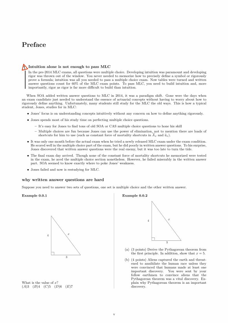
Suppose you need to answer two sets of questions, one set is multiple choice and the other written answer.
Example 0.0.1
3
4 x
What is the value of x?(A)3 (B)4 (C)5 (D)6 (E)7
Example 0.0.2
3
4 x
(a) (3 points) Derive the Pythagorean theorem fromthe first principle. In addition, show that x = 5.
(b) (4 points) Aliens captured the earth and threat-ened to annihilate the human race unless theywere convinced that humans made at least oneimportant discovery. You were sent by yourfollow earthmen to convince aliens that thePythagorean theorem was a vital discovery. Ex-plain why Pythagorean theorem is an importantdiscovery.
v

Example 0.0.3
For a fully discrete whole life insurance of 100,000 on(50), you are given:
(i) The gross premium is calculated under the equiv-alence principle.
(ii) Expenses, payable at the beginning of the year,are:
% of Premium Per PolicyFirst Year 40% 25Renewal 5% 10
(iii) Claim cost: 100 per death.
(iv) Mortality: Illustrative Life Table.
(v) i = 0.06
Calculate the expense premium for this policy.(A)120 (B)170 (C)220 (D)270 (E)320
Calculate the expense premium policy value at theend of Policy Year 10.(A)− 600 (B)− 200 (C)200 (D)600 (E)1, 000
Example 0.0.4
For a fully discrete whole life insurance of 100,000 on(50), you are given:
(i) The gross premium is calculated under the equiv-alence principle.
(ii) Expenses, payable at the beginning of the year,are:
% of Premium Per PolicyFirst Year 40% 25Renewal 5% 10
(iii) Claim cost: 100 per death.
(iv) Mortality: Illustrative Life Table.
(v) i = 0.06
(a) (2 points) Define the expense premium.
(b) (3 points) Show that the prospective expense pre-mium policy value at the end of Policy Year 10 is−600 to the nearest of 10. Explain why the ex-pense premium policy value at the end of PolicyYear 10 is negative.
(c) (2 points) Prove that the retrospective expensepremium policy value and the prospective ex-pense premium policy value at the end of PolicyYear 10 are equal.
The cognitive skill required to solve a written answer question is significantly higher than what is required to solve amultiple choice question.
intuition vs. rigor
Let’s use the concept of the force of mortality and explore the difference between intuitive thinking and rigorous thinking.
What’s the force of mortality? Well, it’s kind of like the force of interest. The force of interest is aninstantaneous rate of increase of your money in a savings account. The force of mortality is an instanta-neous rate of increase of what? Yes, an instantaneous rate of increase of the number of survivors `x or aninstantaneous rate of increase of the survival function.
But wait! There’s a catch. While money grows over time, the survival function decreases over time –people die over time. So we need to add a negative sign to prevent the force of mortality from becomingnegative. No body likes negative numbers. All I need to do is to translate the force of interest formula
A(t) = A(0) exp
(∫ t
0δ(s)ds
).
into the force of mortality formula:
tpx = 0px exp
(−∫ t
0µx(s)ds
)
I got it! What else? Wait! The next formula is like a definition. I shall memorize it.
µx(t) = − d
dtln tpx
That’s about it. I definitely don’t want to clog my head with useless proofs or fancy jargons invented byscholars who live in the cloud. Next, why don’t I solve a bunch of (multiple choice) problems to cement myunderstanding?
Here’s a rigorous approach to the force of mortality:

Let T0 represent the future lifetime of a newborn. Let Tx represent the future lifetime of life aged x. The forceof mortality at age x is represented by µx. We define µx as:
µx = limdx→0+
1dxPr[T0 ≤ x+ dx | T0 > x]
However, Pr[Tx ≤ t] = Pr[T0 ≤ x+ t | T0 > x]
⇒ µx = limdx→0+
1dxPr[Tx ≤ dx]
Let Sx = P (Tx > t) represent the survival function of Tx. The above equation can be rewritten as:
µx = limdx→0+
1dx
(1− Sx(dx)
). . .
While intuitive thinking has served you well in P and FM, it’s no longer sufficient for passing MLC. SOA wants toencourage the next generation of actuaries to be articulate, precise, and resourceful in their professions who can handleanything thrown at them. It doesn’t want to send a bunch of smart calculators to the ASA and FSA destinations.
don’t second guess what SOA will test you
While multiple choice questions tend to be more predictable over time, for written answer questions the sky is the limit.SOA can ask you to do anything, from defining a rudimentary concept such as tpx, to explaining an obscure idea ofzeroized reserves, to the dreaded work of deriving Thiele’s differential equation. To bring this idea home, let’s look atthe following example:
Example 0.0.5
(MLC Fall 2015 Q5) ( 10 points ) Dana buys a Type B universal life contract of 100,000. You are given:
(i)
Policy Year k AnnualPremium
Annual Costof Insurance
Rate Per1000
Percent ofPremiumCharge
AnnualExpenseCharge
SurrenderCharge
1 1000 —— 60% —— ——2 P2 2 10% 10 2003 P3 3 10% 10 100
k ≥ 4 Pk k 5% 10 0
(ii) The credit interest rate is ic = 0.06
(iii) Dana’s account value at the end of year 1 is 165.
(iv) Except as indicated, there are no deaths or surrenders.
(a) (2 points) Show that if P2 were 1000, Dana’s account value at the end of year 2 would be 920 to the nearest 10.You should calculate the account value to the nearest 1.
(b) (2 points) Dana’s account value at the end of year 3 can be expressed as aP2 + bP3 + c. Calculate a, b, and c.
(c) (4 points) In year 2, Dana pays a premium of 1000 with probability 0.6, or 200 with probability 0.4.If he paid 1000 in year 2, then in year 3 he will pay either 1000 with probability 0.6, or 200 with probability 0.4.If he paid 200 in year 2, then in year 3 he will pay either 1000 with probability 0.2, or 200 with probability 0.8.
(i) Calculate the expected death benefit payable at the end of year 3, if Dana dies then.(ii) Calculate the expected surrender benefit payable at the end of year 3, if Dana surrenders the contract then.
(d) (2 points) Dana’s identical twin, Mark, buys a contract identical to Dana’s. If Mark pays 1000 every year, Mark’saccount value at the end of year 10 will be 5114.Mark will pay premiums of 1000 in 9 of the first 10 years. Mark will pay no premium in one year, with the yearof no premium equally likely to be year 3 or year 10.Calculate Mark’s expected surrender value at the end of year 10.
The setup of this question, especially Part (b), (c), and (d), is simply the work of a genius. You have a better chanceof getting struck by lightning than guessing that SOA will test your UL account value this way. To score this problem,you just have to know the UL account value inside out. Now memorized shortcut can save you.
how to prepare for written answer questions
First, from Day One, say goodbye to the pure intuition based learning and embrace rigor in your study. Learn how todefine and derive. Build a new habit of showing your work so a random grader can follow your steps.
Next, embrace the pain of studying for MLC. There’s no shortcut to learning policy values, profit testing, or anyother major concept in MLC. You just have to spend a lot of time learning major concepts and solving problems.
vii c© Yufeng Guo, MLC Fall 2017

how this book can help you
Imagine that you are to play a chess with a devil. If you win at least 6 out of 10 games, you move on with your life.Otherwise, your life comes to screeching halt and you go to your basement to relearn chess and prepare for anothermatch. How can you beat the devil?
The only thing I can think of is to become a well-rounded chess player. Play a lot of games and experience a lot offighting scenarios so you can adapt to change.
In this book, I throw you into a wide range of problems, some written answer and others multiple choice stylequestions. The goal is to help you build both intuition and rigor necessary for passing MLC.
Before writing this book, I went through the SOA syllabus and the AMLCR textbook and identified the majorconcepts you need to learn to score well in both the written answer questions and the multiple choice questions for theexam. I then wrap these concepts in a series of problems.
In each chapter, I’ll teach you how to solve one major type of written answer or multiple choice questions. If you canmaster the problems in my book, you’ll have gained a sophisticated understanding of the core concepts and should beable to tackle most problems SOA throws at you, whether the questions are multiple choice or written answer ones.
My story
I came to U.S. from China when I was in my late twenties. I started my first corporate job in U.S. in the IT departmentof a large insurance company. After working there for about 2 years, I was ready to switch my career. If you have everworked in a large IT department or any large department of a large company, you’ll find that there are thousands ofpeople just like you who go to the same building in the morning around the same time you go to the building and wholeave the same building in the afternoon around the same time you leave the building. The company’s giant parking lotswere filled with thousands of cars, one of which was my second hand red Toyota Camry. The building is nice. Coworkersare nice. But I felt like a drop of water in the ocean.
I was floating around not sure how to make use of my life. Then one day I heard the actuary profession. I heardthat if you were an actuary, you were among the elite group because there weren’t enough actuaries to go around. Iwas interested. I decided to study for P. By that time, I hadn’t touched calculus for 13 years. Fortunately, it took mejust a couple of months to relearn calculus. I took P and got a 9. I was overjoyed. I applied for a job in the actuarydepartment and became an actuary.
When I became an entry level actuary, I was in my early 30’s, about 8 years older than most of my peers, who got theactuary job straight from college. To quickly pass actuary exams, I used a bold strategy: reverse engineering. This isnot for the faint of the heart. Think twice before you try it. It works like this. Before I took an exam, say MLC, I useda company printer and printed out all the released MLC exam papers and the official solution papers. There was a stackof paper on my desk. From the stack, I pulled out the most recent exam paper, looked up the SOA solutions, looked upthe subject from the textbook, and studied the subject. Then I moved to the next exam paper. I call this just-in-timestudy, similar to the just-in-time inventory method used in Toyota and many other auto manufacturing plants aroundthe world.
It typically took me two to three months to master all the released papers. When the final exam day came, I walkedinto the exam room. You know what I saw? Sure there were surprise problems, but most exam problems were just likethe problems tested before. I was able to solve those similar problems pretty much 100% right. I just passed anotherexam.
However, since written answer questions were added in 2014 and there aren’t many released written answer questionsto master. My old strategy may not work any more.
how to pass MLC or any actuary exam
Based on my experience of studying for actuary exams, I firmly believe that to pass an actuary exam you need to do 2things: (1) you have to understand the core concepts, and (2) you have to be able to quickly solve the types of problemsSOA likes to test.
Building a coherent body of knowledge of the subject matter is the most critical and the most time-consuming partof studying for an actuary exam. If you walk into the exam room muddleheaded or with scanty knowledge of basictheories, none of the tips or tricks you learned from an exam prep book would save you. Any chess master will tell youthat there are no shortcuts in learning chess. You just have to know your stuff!
However, knowing the subject well doesn’t guarantee passing the exam or earning a high grade any more than goodtechnical skills guarantee a job offer. It’s a sad reality that often those who know how to play the interview game get thejob. When you take actuary exams, your knowledge is measured by your ability to solve the SOA style questions. Topass MLC, you’ll need to immerse yourself in the types of problems SOA likes to test or you’ll be one of those “theorysmart, exam poor” people.
One key part of studying the SOA exam papers is to identify commonly tested problem types and learn how to solvethem quickly. For example, finding the UL account value is tested in virtually every exam. Your first round of effort isto understand what is UL, what is Type A and Type B, what is COI, what is corridor, and how the UL account valuebuilds up over time. After you understand these basic concepts, you face a choice about how to find the Type A ULaccount value. Should you solve two linear equations on AVt and COIt or should you memorize the formulas for AVtand COIt to avoid having to solve two equations in the exam? You might try both approaches and see which methodsuits you. You might find that there’s no clear winner and that you want to learn both. However, before taking theexam, you must have a tried-and-true procedure for calculating the Type A UL account value. You don’t want to walkinto exam empty handed without a proven method in your head.
Here’s the final point. It’s not absolutely necessary, but it helps. Most people’s performance will downgrade in theheat of the exam. To be safe, strive to learn at least a little bit more than the minimal knowledge required to pass MLC.When I was studying an old exam paper, I often asked myself “How can I make this problem harder?” If I saw a subjectthat was in the syllabus but that was not tested in the past, I often forced myself to learn at least a little bit aboutit. Even if the subject didn’t show up in the test, knowing that I was not a complete idiot on the subject reduced myanxiety.
know your stuff
Google Maps are handy especially when you go to a new place, but I hope you know how to get to your work or schoolwhen you left your phone at home or there’s no internet connection. Over the years, I have developed many alternativeroutes for my daily commute. If route A is closed, I know what an alternative route to go. I know which road tendsto be jammed by school buses, which road is more likely to have accidents, which alley is slippery when it snows. Thisknowledge serves me well. Just the other day, while I was driving to work, the road I took had a car accident. Whilemost drivers were stuck in the traffic, I knew the exact small neighborhood that I needed to turn to bypass the trafficjam.
In virtually every career you choose, there’s no substitute for learning the basics for doing the job. To study for MLC,you just have to learn the fundamentals: the force of mortality, the multiple state model, profit testing, to name a few.
When I was a college student in China, one day I found a great shortcut for learning English. I’m sure many of youhave attempted, at some point in your life, to be very good at a foreign language that is fundamentally differentfrom your native language. A foreign language is like a bottomless pit. No matter how much effort you put intoit, you almost always end up going nowhere. You are good enough to say “How are you?” but never be able tounderstand a movie. You are so angry with yourself and with the foreign language.
Anyway, one day I had a great revelation. If I could spend a year memorizing an English dictionary, I wouldmaster the English language once for all! The first few weeks were great. I felt my vocabulary grew exponentiallyat least for the words that started with the letter A. However, two months later my balloon of hope was punctured.I couldn’t move beyond the letter A. And I forgot most of the words I learned. I went back to square one.
man’s never-ending quest for shortcuts
There are shortcuts for solving some problems in MLC (such as constant force of mortality shortcuts). However,there’s no shortcut for building a coherent body of knowledge for life contingency theories. You just have to learnone concept at a time. You just have to cycle through the major MLC concepts several times to achieve sophisticatedunderstanding.
Most of you reading this book should plan to spend at least 3 months to study for MLC. Learning takes time. Thatsaid, if you are a high achiever or you got a 5 last time and are re-taking MLC, 2 months might be enough.
a simple procedure beats the best mind
I remember a story I learned from a computer programming book. The story goes like this. A town in the Midwesthas two coffee shops, A and B. If you visit Shop A, sometimes you can get coffee right away but other times they runout of coffee and you have to wait a little while. Shop B, on the other hand, always has coffee ready for a customerwho just walks in. Both shops are in the same town and their workers have roughly the same skills. How does Shop Boutsmart Shop A? In turns out that Shop B has a simple procedure. If you work in Shop B, from Day One you learnthis rule: when existing coffee in a container reaches a certain low level, stop whatever you are doing and immediatelystart brewing new coffee. This procedure makes all the difference.
A procedure in programming is called an algorithm. When studying for an actuary exam, you’ll need to buildalgorithms for commonly tested problems to avoid having to reinvent the wheel in the heat of the exam. When the bigexam day comes, most of the problem types in the exam should be familiar to you and your job is just to recall pre-builtalgorithms. Don’t purposely put yourself on the spot without an algorithm for finding the Type A UL account value.You have only several minutes per exam problem and in the heat of the exam it’s really hard to invent a solution to anunseen problem type.
acknowledgement
First, I want to thank two actuaries, Nathan Hardiman and Robin Cunningham, for their generosity. They gave metheir Arch manual for the then Course 3 or Exam M practically free. Years ago they wrote a really good study manualcalled Arch for the then MLC. You might not know that of all the exams for ASA, MLC changes most frequently. Forexample, if you dig through old Course 3 exam papers, you’ll find the famous problem of “Lucky Tom finds coins at thePoisson rate of ... per hour.” The Poisson distribution or Poisson process was a hot topic dreaded by many. To yourrelief, SOA dropped the Poisson process from the syllabus. Anyway, Nathan and Robin have their full time corporateactuarial jobs and couldn’t keep up with frequent changes in the exam syllabus. Instead of withdrawing their Arch bookfrom the market and letting their brain child die, they decided to give the Arch manual to another author. Since I wrotemany study manuals, they gave me the book.
The Arch manual was a turning point for me technically. After downloading their manuscript from my email, I foundout that Arch was written in LATEX, not in Word. That was the first time I saw LATEX code. At at time, I was lookingfor a solution to a long standing problem of Word crashing on me. Arch was a god sent. From Arch, I learned LATEXand switched from Word to LATEX for my future books.
In addition, I want to thank the many LATEX contributors for their wonderful packages. Without LATEX or many ofits special packages, this book isn’t possible.
Finally, I think you, dear reader, for reading the thoughts and reasoning I came up with after my actuarial day job.I hope you find this book useful. If you end up using this book, I thank you for the opportunity of being part of yourjourney into the actuarial dream land.
outlook of actuary profession
According to the U.S. Bureau of Labor Statistics, employment of actuaries is projected to grow 18% from 2014 to 2024,much faster than the average for all occupations. What are you waiting for? Study for MLC today!
ix c© Yufeng Guo, MLC Fall 2017

FAQ
Does this book cover the entire syllabus?Yes. The entire syllabus is covered.
Is this book sufficient for passing MLC?No author can guarantee that if you read his book you will surely pass MLC. That said, if you can master thisbook and master the SOA exam papers, you have built a solid foundation for passing MLC.
What companion book do you recommend to use along side with this book?I recommend that you can use this book together with the AMLCR textbook and the SOA exam papers.
errata
Sample chapters and the errata for this book can be found at http://deeperunderstandingfastercalc.com/mlc-solver.php

Chapter 48
Multiple state model: write down Kolmogorov’s forwardequations 100% right in a hurry
One major pain point that many exam candidates have is to correctly write down the Kolmogorov’s forward equationsin the heat of the exam. A minor pain point is to write down the associated boundary conditions for the Kolmogorov’sforward equations. Today we’re going to put an end to these struggles. After reading this chapter, you’ll be able towrite down the Kolmogorov’s forward equations and the boundary conditions 100% correct in a hurry.
Example 48.0.1
A combined disability and critical illness policy is issued to a healthy life age x. Write down the Kolmogorov’s forwardequations and the boundary conditions for
(a) tp00x
(b) tp01x
(c) tp02x
(d) tp03x
Healthy Sick
Dead Critically ill
0 1
2 3
µ01x+t
µ10x+t
µ02x+t
µ13x+t
µ32x+t
µ12x+tµ03
x+t
Solution 48.0.1
(a) Write down the Kolmogorov’s forward equation for tp00x .
Step 1. For each node j where j = 0, 1, 2, 3, change the name of the node from j to 0j.
Healthy Sick
Dead Critically ill
00 01
02 03
µ01x+t
µ10x+t
µ02x+t
µ13x+t
µ32x+t
µ12x+tµ03
x+t
We interpret each node as follows: at t = 0, the universe has 1 healthyperson (ancestor) and no one else. This person’s offsprings fill the uni-verse. The population of this universe is always one at any time. Un-fortunately, the offspring population isn’t growing, unlike Abraham’schildren. At t, we count the people in the universe.
• In the node name 0j, 0 is the ancestor’s name; j is the offspring’sname.
• tp00x is the (expected) number of the healthy people at t.
• tp01x is the (expected) number of the sick people at t.
• tp02x is the (expected) number of the dead people at t.
• tp03x is the (expected) number of the critically ill people at t.
• The total population at t is tp00x + tp
01x + tp
02x + tp
03x = 1.
Step 2. From all the nodes, isolate the nodes that point to the node 00. The insureds in these nodes can flow into thenode 00, causing d
dttp
00x to increase.
387

Healthy Sick
00 01
µ10x+t
positive forces of d
dttp
00x : tp
01x µ
10x+t
Step 3. From all the nodes, isolate the nodes that are pointed to by the node 00. The insureds in the node 00 canflow into these nodes, causing d
dttp
00x to decrease.
Healthy Sick
Dead Critically ill
00 01
02 03
µ01x+t
µ02x+t
µ03x+t
negative forces of d
dttp
00x : −tp00
x
(µ01x+t + µ02
x+t + µ03x+t)
Step 4: Combine the positive and the negative forces and you’ll get the Kolmogorov’s forward equation.
Healthy Sick
Dead Critically ill
0 1
2 3
µ01x+t
µ10x+t
µ02x+t
µ13x+t
µ32x+t
µ12x+tµ03
x+t
d
dttp
00x = tp
01x µ
10x+t − tp
00x
(µ01x+t + µ02
x+t + µ03x+t)
The boundary condition is either the beginning condition or the ending condition. Since at time zero, the insured ishealthy, the boundary conditions are
0p00x = 1, 0p
01x = 0p
02x = 0p
03x = 0
(b) Write down the Kolmogorov’s forward equation for tp01x . Isolate the positive forces (the nodes that can flow into
the node 01):
Healthy Sick
00 01
µ01x+t
positive forces of d
dttp
01x : tp
00x µ
01x+t
Isolate the negative forces (the nodes that the node 01 can flow into):

Healthy Sick
Dead Critically ill
00 01
02 03
µ10x+t
µ12x+t µ13
x+t
negative forces of d
dttp
01x : −tp01
x
(µ10x+t + µ12
x+t + µ13x+t)
Combine the positive and the negative forces:
Healthy Sick
Dead Critically ill
0 1
2 3
µ01x+t
µ10x+t
µ02x+t
µ13x+t
µ32x+t
µ12x+tµ03
x+t
d
dttp
01x = tp
00x µ
01x+t − tp
01x
(µ10x+t + µ12
x+t + µ13x+t)
boundary condition: 0p00x = 1, 0p
01x = 0p
02x = 0p
03x = 0
(c) Write down the Kolmogorov’s forward equation for tp02x . Isolate all the nodes that can flow into the node 02:
Healthy Sick
Dead Critically ill
00 01
02 03
µ02x+t
µ32x+t
µ12x+t
positive forces: d
dttp
02x : tp
00x µ
02x+t + tp
01x µ
12x+t + tp
03x µ
32x+t
There are no negative forces that will pull the insured away from the 02 node. The population in the node 02 can onlyincrease.
d
dttp
02x = tp
00x µ
02x+t + tp
01x µ
12x+t + tp
03x µ
32x+t
boundary condition: 0p00x = 1, 0p
01x = 0p
02x = 0p
03x = 0
(d) Write down the Kolmogorov’s forward equation for tp03x .
389 c© Yufeng Guo, MLC Fall 2017

Healthy Sick
Critically ill
00 01
03
µ13x+t
µ03x+t
positive forces: d
dttp
03x : tp
00x µ
03x+t + tp
01x µ
13x+t
Dead Critically ill
02 03µ32x+t
negative forces: d
dttp
03x : −tp03
x µ32x+t
⇒ d
dttp
03x = tp
00x µ
03x+t + tp
01x µ
13x+t − tp
03x µ
32x+t
boundary condition: 0p00x = 1, 0p
01x = 0p
02x = 0p
03x = 0
Example 48.0.2
(Same model as before but repeated for convenience) A combined disability and critical illness policy is issued to ahealthy life age x. Write down the Kolmogorov’s forward equations for
(a) tp10x
(b) tp11x
(c) tp12x
(d) tp13x
Healthy Sick
Dead Critically ill
0 1
2 3
µ01x+t
µ10x+t
µ02x+t
µ13x+t
µ32x+t
µ12x+tµ03
x+t
Solution 48.0.2
The process is the same as that in the previous problem. First, we relabel each node as 1j.
Healthy Sick
Dead Critically ill
10 11
12 13
µ01x+t
µ10x+t
µ02x+t
µ13x+t
µ32x+t
µ12x+tµ03
x+t
We interpret each node as follows: at some point before t, the universehas only 1 sick person (ancestor). This person’s children fill the universe.At t, we count the people in the universe.
• In the node name 1j, 1 is the ancestor’s name; j is the offspring’sname.
• tp10x is the (expected) number of the healthy people at t.
• tp11x is the (expected) number of the sick people at t.
• tp12x is the (expected) number of the dead people at t.
• tp13x is the (expected) number of the critically ill people at t.
• The total population at t is tp10x + tp
11x + tp
12x + tp
13x = 1.

(a)
Healthy Sick
10 11
µ10x+t
positive forces: d
dttp
10x : tp
11x µ
10x+t
Healthy Sick
Dead Critically ill
10 11
12 13
µ01x+t
µ02x+t
µ03x+t
negative forces: d
dttp
10x : −tp10
x
(µ01x+t + µ02
x+t + µ03x+t)
⇒ d
dttp
10x = tp
11x µ
10x+t − tp
10x
(µ01x+t + µ02
x+t + µ03x+t)
(b)
Healthy Sick
10 11
µ01x+t positive forces: d
dttp
11x : tp
10x µ
01x+t
Healthy Sick
Dead Critically ill
10 11
12 13
µ10x+t
µ13x+t
µ12x+t
negative forces: d
dttp
11x : −tp11
x
(µ10x+t + µ12
x+t + µ13x+t)
⇒ d
dttp
11x = tp
10x µ
01x+t − tp
11x
(µ10x+t + µ12
x+t + µ13x+t)
(c) There are only positive forces for the node 12:
Healthy Sick
Dead Critically ill
10 11
12 13
µ02x+t
µ32x+t
µ12x+t
d
dttp
12x = tp
10x µ
02x+t + tp
11x µ
12x+t + tp
13x µ
32x+t
391 c© Yufeng Guo, MLC Fall 2017
(d)
Healthy Sick
Critically ill
10 11
13
µ13x+t
µ03x+t
positive forces: d
dttp
13x : tp
10x µ
03x+t + tp
11x µ
13x+t
Dead Critically ill
12 13µ32x+t
negative forces: d
dttp
13x : −tp13
x µ32x+t
⇒ d
dttp
13x = tp
10x µ
03x+t + tp
11x µ
13x+t − tp
13x µ
32x+t
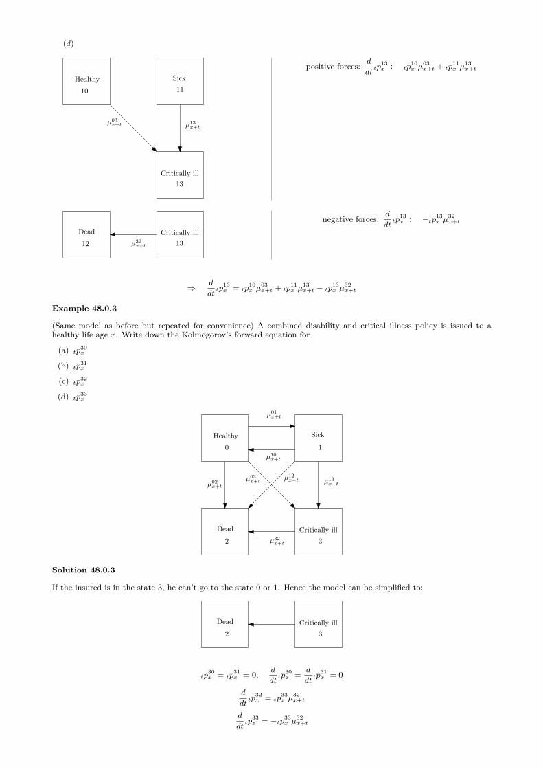
Example 48.0.3
(Same model as before but repeated for convenience) A combined disability and critical illness policy is issued to ahealthy life age x. Write down the Kolmogorov’s forward equation for
(a) tp30x
(b) tp31x
(c) tp32x
(d) tp33x
Healthy Sick
Dead Critically ill
0 1
2 3
µ01x+t
µ10x+t
µ02x+t
µ13x+t
µ32x+t
µ12x+tµ03
x+t
Solution 48.0.3
If the insured is in the state 3, he can’t go to the state 0 or 1. Hence the model can be simplified to:
Dead Critically ill
2 3
tp30x = tp
31x = 0, d
dttp
30x = d
dttp
31x = 0
d
dttp
32x = tp
33x µ
32x+t
d
dttp
33x = −tp33
x µ32x+t

Example 48.0.4
(Same model as before but repeated for convenience) A combined disability and critical illness policy is issued to ahealthy life age x. Write down the Kolmogorov’s forward equations for
(a) tp20x
(b) tp21x
(c) tp22x
(d) tp23x
Healthy Sick
Dead Critically ill
0 1
2 3
µ01x+t
µ10x+t
µ02x+t
µ13x+t
µ32x+t
µ12x+tµ03
x+t
Solution 48.0.4
If the insured is currently in the state 2, he’ll be stuck in the state 2 and can’t go to the state 0, 1 or 3. The model canbe simplified to:
Dead
2
tp20x = tp
21x = tp
23x = 0, tp
22x = 1
⇒ d
dttp
20x = d
dttp
21x = d
dttp
22x = d
dttp
23x = 0
Example 48.0.5
(Same model as before but repeated for convenience) A combined disability and critical illness policy is issued to ahealthy life age x. The insured is currently in the state 0. Explain why
d
dttp
00x + d
dttp
01x + d
dttp
02x + d
dttp
03x = 0
Healthy Sick
Dead Critically ill
0 1
2 3
µ01x+t
µ10x+t
µ02x+t
µ13x+t
µ32x+t
µ12x+tµ03
x+t
Solution 48.0.5
Since the total population is always one, the total change of the population is always zero. Similarly,
d
dttp
10x + d
dttp
11x + d
dttp
12x + d
dttp
13x = 0
d
dttp
20x + d
dttp
21x + d
dttp
22x + d
dttp
23x = 0
d
dttp
30x + d
dttp
31x + d
dttp
32x + d
dttp
33x = 0
393 c© Yufeng Guo, MLC Fall 2017

48.1 Check your knowledge
Homework 48.1.1
Write down the formula for d
dttp
01x .
Healthy Sick
Dead
0 1
2
µ10x
µ01x
µ 02x µ12x
Homework Solution 48.1.1
Difficultyd
dttp
01x = tp
00x µ
01x+t − tp
01x (µ10
x+t + µ12x+t)
Homework 48.1.2
Write down the formula for d
dttp
00x .
Healthy Sick
Dead
0 1
2
µ10x
µ01x
µ 02x µ12x
Homework Solution 48.1.2
Difficulty
d
dttp
00x = tp
01x µ
10x+t − tp
00x (µ01
x+t + µ02x+t)
Homework 48.1.3
Write down the formula for d
dttp
22x .
Healthy Sick
Dead
0 1
2
µ10x
µ01x
µ 02x µ12x
Homework Solution 48.1.3
Difficultyd
dttp
22x = 0
Homework 48.1.4
Write down the formula for d
dttp
10x , d
dttp
12x , d
dttp
02x .
Healthy Sick
Dead
0 1
2
µ10x
µ01x
µ 02x µ12x
Homework Solution 48.1.4
Difficulty
d
dttp
10x = tp
11x µ
10x+t − tp
10x (µ01
x+t + µ02x+t)
d
dttp
12x = tp
11x µ
12x+t + tp
10x µ
02x+t
d
dttp
02x = tp
00x µ
02x+t + tp
01x µ
12x+t
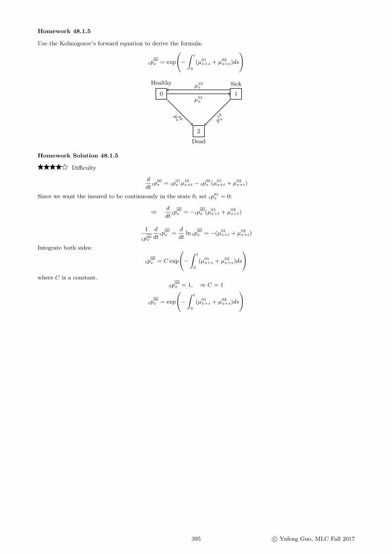
Homework 48.1.5
Use the Kolmogorov’s forward equation to derive the formula:
tp00x = exp
(−∫ t
0(µ01x+s + µ02
x+s)ds
)
Healthy Sick
Dead
0 1
2
µ10x
µ01x
µ 02x µ12x
Homework Solution 48.1.5
Difficulty
d
dttp
00x = tp
01x µ
10x+t − tp
00x (µ01
x+t + µ02x+t)
Since we want the insured to be continuously in the state 0, set tp01x = 0:
⇒ d
dttp
00x = −tp00
x (µ01x+t + µ02
x+t)
1tp00x
d
dttp
00x = d
dtln tp00
x = −(µ01x+t + µ02
x+t)
Integrate both sides:
tp00x = C exp
(−∫ t
0(µ01x+s + µ02
x+s)ds
)where C is a constant.
0p00x = 1, ⇒ C = 1
tp00x = exp
(−∫ t
0(µ01x+s + µ02
x+s)ds
)
395 c© Yufeng Guo, MLC Fall 2017


Chapter 49
Multiple state model: Euler’s method for probabilities
Example 49.0.1
A combined disability and critical illness policy is issued to a healthy life age x. Let h = 1/12 (e.g. one month timestep). Use the Euler’s method and estimate the following probabilities:
(a) hp00x
(b) hp01x
(c) hp02x
(d) hp03x
Healthy Sick
Dead Critically ill
0 1
2 3
µ01x+t = 0.004
µ10x+t = 0.0008
µ02x+t = 0.0005(1 + t) µ13
x+t = 0.0006
µ32x+t
µ12x+tµ03
x+t
µ03x+t = 0.0004
µ12x+t = µ02
x+t = 0.0005(1 + t)
µ32x+t = 2µ02
x+t = 0.001(1 + t)
Solution 49.0.1
The boundary conditions are:0p
00x = 1, 0p
01x = 0p
02x = 0p
03x = 0
(a)d
dttp
00x = tp
01x µ
10x+t − tp
00x
(µ01x+t + µ02
x+t + µ03x+t)
⇒(d
dttp
00x
)t=0
= 0p01x µ
10x+0 − 0p
00x
(µ01x+0 + µ02
x+0 + µ03x+0)
= 0µ10x+0 − 1
(µ01x+0 + µ02
x+0 + µ03x+0)
= 0− 1(0.004 + 0.0005(1 + 0) + 0.0004
)= −0.0049
hp00x ≈ 0p
00x + h
(d
dttp
00x
)t=0
= 1 + 112 × (−0.0049) = 0.99959167
(b)
d
dttp
01x = tp
00x µ
01x+t − tp
01x
(µ10x+t + µ12
x+t + µ13x+t)
(d
dttp
01x
)t=0
= 0p00x µ
01x+0 − 0p
01x
(µ10x+0 + µ12
x+0 + µ13x+0)
= µ01x+0 = 0.004
hp01x ≈ 0p
01x + h
(d
dttp
01x
)t=0
= 0 + 112 × 0.004 = 0.00033333
(c)
397

d
dttp
02x = tp
00x µ
02x+t + tp
01x µ
12x+t + tp
03x µ
32x+t(
d
dttp
02x
)t=0
= 0p00x µ
02x+0 + 0p
01x µ
12x+0 + 0p
03x µ
32x+0
= µ02x+0 = 0.0005(1 + 0) = 0.0005
hp03x ≈ 0p
03x + h
(d
dttp
03x
)t=0
= 0 + 112 × 0.0005 = 0.00004167
(d)
d
dttp
03x = tp
00x µ
03x+t + tp
01x µ
13x+t − tp
03x µ
32x+t(
d
dttp
03x
)t=0
= 0p00x µ
03x+0 + 0p
01x µ
13x+0 − 0p
03x µ
32x+0
= µ03x+0 = 0.0004
hp03x ≈ 0p
03x + h
(d
dttp
03x
)t=0
= 0 + 112 × 0.0004 = 0.00003333
Check: 0.99959167 + 0.00033333 + 0.00004167 + 0.00003333 = 1 OK
Example 49.0.2
(Same model as before but repeated for convenience) A combined disability and critical illness policy is issued to ahealthy life age x. Let h = 1/12 (e.g. one month time step). Use the Euler’s method and estimate the followingprobabilities:
(a) 2hp00x
(b) 2hp01x
(c) 2hp02x
(d) 2hp03x
Healthy Sick
Dead Critically ill
0 1
2 3
µ01x+t = 0.004
µ10x+t = 0.0008
µ02x+t = 0.0005(1 + t) µ13
x+t = 0.0006
µ32x+t
µ12x+tµ03
x+t
µ03x+t = 0.0004
µ12x+t = µ02
x+t = 0.0005(1 + t)
µ32x+t = 2µ02
x+t = 0.001(1 + t)
You are given: hp00x = 0.99959167, hp01
x = 0.00033333, hp02x = 0.00004167, and hp
03x = 0.00003333
Solution 49.0.2
(a)d
dttp
00x = tp
01x µ
10x+t − tp
00x
(µ01x+t + µ02
x+t + µ03x+t)
⇒(d
dttp
00x
)t=h
= hp01x µ
10x+h − hp
00x
(µ01x+h + µ02
x+h + µ03x+h)
= 0.00033333× 0.0008− 0.99959167(0.004 + 0.0005(1 + 1/12) + 0.0004
)= −0.00493938
2hp00x ≈ hp
00x + h
(d
dttp
00x
)t=h
= 0.99959167 + 112 × (−0.00493938) = 0.99918006
(b)
d
dttp
01x = tp
00x µ
01x+t − tp
01x
(µ10x+t + µ12
x+t + µ13x+t)
(d
dttp
01x
)t=h
= hp00x µ
01x+h − hp
01x
(µ10x+h + µ12
x+h + µ13x+h)
= 0.99959167× 0.004− 0.00033333(0.0008 + 0.0005(1 + 1/12) + 0.0006
)= 0.00399772
2hp01x ≈ hp
01x + h
(d
dttp
01x
)t=h
= 0.00033333 + 112 × (0.00399772) = 0.000666473
(c)
d
dttp
02x = tp
00x µ
02x+t + tp
01x µ
12x+t + tp
03x µ
32x+t(
d
dttp
02x
)t=h
= hp00x µ
02x+h + hp
01x µ
12x+h + hp
03x µ
32x+h
= 0.99959167× 0.0005(1 + 1/12) + 0.00033333× 0.0005(1 + 1/12) + 0.00003333× 0.001(1 + 1/12)
= 0.00054166
2hp02x ≈ hp
02x + h
(d
dttp
02x
)t=h
= 0.00004167 + 112 × 0.00054166 = 0.00008700
(d)
d
dttp
03x = tp
00x µ
03x+t + tp
01x µ
13x+t − tp
03x µ
32x+t(
d
dttp
03x
)t=h
= hp00x µ
03x+h + hp
01x µ
13x+h − hp
03x µ
32x+h
= 0.99959167× 0.0004 + 0.00033333× 0.0006− 0.00003333× 0.001(1 + 1/12)
= 0.00040000
2hp03x ≈ hp
03x + h
(d
dttp
03x
)t=h
= 0.00003333 + 112 × 0.00040000 = 0.00006663
Check: 0.99918006 + 0.000666473 + 0.00008700 + 0.00006663 = 1.0000002 ≈ 1 OK
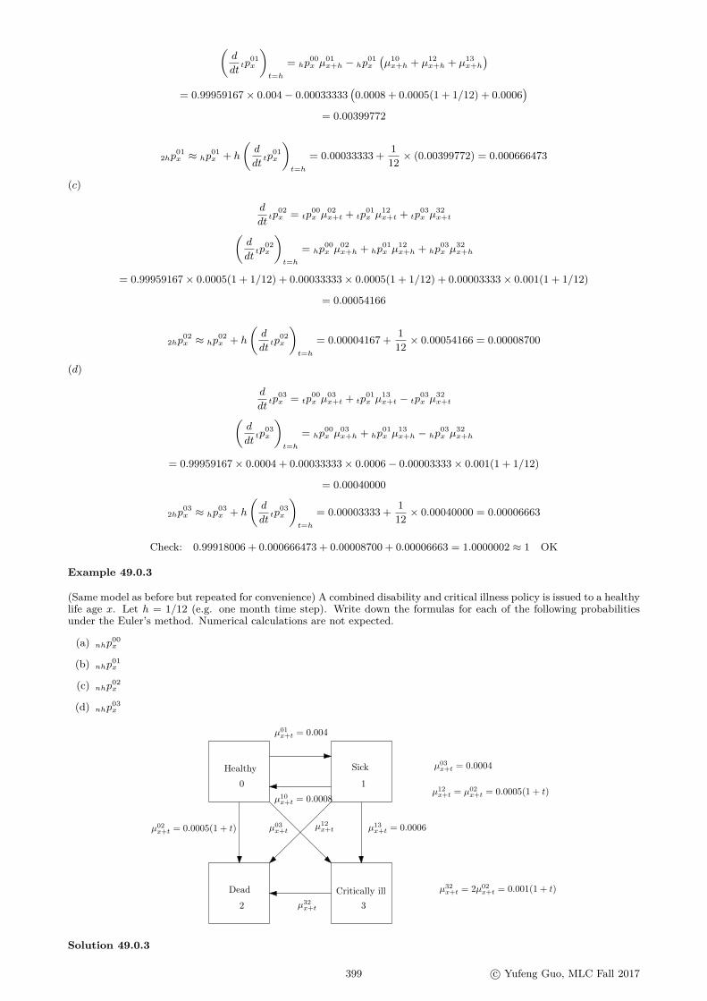
Example 49.0.3
(Same model as before but repeated for convenience) A combined disability and critical illness policy is issued to a healthylife age x. Let h = 1/12 (e.g. one month time step). Write down the formulas for each of the following probabilitiesunder the Euler’s method. Numerical calculations are not expected.
(a) nhp00x
(b) nhp01x
(c) nhp02x
(d) nhp03x
Healthy Sick
Dead Critically ill
0 1
2 3
µ01x+t = 0.004
µ10x+t = 0.0008
µ02x+t = 0.0005(1 + t) µ13
x+t = 0.0006
µ32x+t
µ12x+tµ03
x+t
µ03x+t = 0.0004
µ12x+t = µ02
x+t = 0.0005(1 + t)
µ32x+t = 2µ02
x+t = 0.001(1 + t)
Solution 49.0.3
399 c© Yufeng Guo, MLC Fall 2017

(a)d
dttp
00x = tp
01x µ
10x+t − tp
00x
(µ01x+t + µ02
x+t + µ03x+t)
⇒(d
dttp
00x
)t=(n−1)h
= (n−1)hp01x µ
10x+(n−1)h − (n−1)hp
00x
(µ01x+(n−1)h + µ02
x+(n−1)h + µ03x+(n−1)h
)nhp
00x ≈ (n−1)hp
00x + h
(d
dttp
00x
)t=(n−1)h
(b)
d
dttp
01x = tp
00x µ
01x+t − tp
01x
(µ10x+t + µ12
x+t + µ13x+t)
(d
dttp
01x
)t=(n−1)h
= (n−1)hp00x µ
01x+(n−1)h − (n−1)hp
01x
(µ10x+(n−1)h + µ12
x+(n−1)h + µ13x+(n−1)h
)nhp
01x ≈ (n−1)hp
01x + h
(d
dttp
01x
)t=(n−1)h
(c)
d
dttp
02x = tp
00x µ
02x+t + tp
01x µ
12x+t + tp
03x µ
32x+t(
d
dttp
02x
)t=(n−1)h
= (n−1)hp00x µ
02x+(n−1)h + (n−1)hp
01x µ
12x+(n−1)h + (n−1)hp
03x µ
32x+(n−1)h
nhp02x ≈ (n−1)hp
02x + h
(d
dttp
02x
)t=(n−1)h
(d)
d
dttp
03x = tp
00x µ
03x+t + tp
01x µ
13x+t − tp
03x µ
32x+t(
d
dttp
03x
)t=(n−1)h
= (n−1)hp00x µ
03x+(n−1)h + (n−1)hp
01x µ
13x+(n−1)h − (n−1)hp
03x µ
32x+(n−1)h
nhp03x ≈ (n−1)hp
03x + h
(d
dttp
03x
)t=(n−1)h
Example 49.0.4
(Same model as before but repeated for convenience) A combined disability and critical illness policy is issued to ahealthy life age x. Let h = 1/12 (e.g. one month time step). Use the Euler’s method and estimate the followingprobabilities:
(a) hp10x
(b) hp11x
(c) hp12x
(d) hp13x
Healthy Sick
Dead Critically ill
0 1
2 3
µ01x+t = 0.004
µ10x+t = 0.0008
µ02x+t = 0.0005(1 + t) µ13
x+t = 0.0006
µ32x+t
µ12x+tµ03
x+t
µ03x+t = 0.0004
µ12x+t = µ02
x+t = 0.0005(1 + t)
µ32x+t = 2µ02
x+t = 0.001(1 + t)
Solution 49.0.4

It may strike you as absurd to calculate these probabilities given that at time zero (e.g. contract initiation) the insuredis in the state 0. However, we can still compile these probabilities by arbitrarily assuming that the insured is in the state1 at time zero. The boundary conditions for these probabilities are:
0p11x = 1, 0p
10x = 0p
12x = 0p
13x = 0
(a)d
dttp
10x = tp
11x µ
10x+t − tp
10x
(µ01x+t + µ02
x+t + µ03x+t)
⇒(d
dttp
10x
)t=0
= 0p11x µ
10x+0 − 0p
10x
(µ01x+0 + µ02
x+0 + µ03x+0)
= 1× µ10x+0 − 0
(µ01x+0 + µ02
x+0 + µ03x+0)
= µ10x+0 = 0.0008
hp01x ≈ 0p
01x + h
(d
dttp
01x
)t=0
= 0 + 112 × 0.0008 = 0.00006667
(b)
d
dttp
11x = tp
10x µ
01x+t − tp
11x
(µ10x+t + µ12
x+t + µ13x+t)
(d
dttp
11x
)t=0
= 0p10x µ
01x+0 − 0p
11x
(µ10x+0 + µ12
x+0 + µ13x+0)
= −(µ10x+0 + µ12
x+0 + µ13x+0)
= −(0.0008 + 0.0005(1 + 0) + 0.0006
)= −0.00190000
hp11x ≈ 0p
11x + h
(d
dttp
11x
)t=0
= 1 + 112 × (−0.00190000) = 0.99984167
(c)
d
dttp
12x = tp
10x µ
02x+t + tp
11x µ
12x+t + tp
13x µ
32x+t(
d
dttp
12x
)t=0
= 0p10x µ
02x+0 + 0p
11x µ
12x+0 + 0p
13x µ
32x+0
= µ12x+0 = 0.0005(1 + 0) = 0.0005
hp12x ≈ 0p
12x + h
(d
dttp
12x
)t=0
= 0 + 112 × 0.0005 = 0.00004167
(d)
d
dttp
13x = tp
10x µ
03x+t + tp
11x µ
13x+t − tp
13x µ
32x+t(
d
dttp
13x
)t=0
= 0p10x µ
03x+0 + 0p
11x µ
13x+0 − 0p
13x µ
32x+0
= µ13x+0 = 0.0006
hp13x ≈ 0p
13x + h
(d
dttp
13x
)t=0
= 0 + 112 × 0.0006 = 0.00005
Check: 0.00006667 + 0.99984167 + 0.00004167 + 0.00005 = 1 OK
401 c© Yufeng Guo, MLC Fall 2017

49.1 Check your knowledge
Homework 49.1.1
You are given the following model (AMLCR textbook Example 8.5):
• µ01x = a1 + b1 exp(c1x), µ10
x = 0.1µ01x , µ02
x = a2 + b2 exp(c2x), µ12x = µ02
x
• a1 = 0.0004, b1 = 3.4674× 10⁻⁶, c1 = 0.138155
• a2 = 0.0005, b2 = 7.5858× 10⁻⁵, c2 = 0.087498
Healthy Sick
Dead
0 1
2
µ10x
µ01x
µ 02x µ12x
Let h = 1/12 and x = 60.
(a) Briefly explain why it’s difficult or impossible to find an exact formula for hp00x .
(b) Briefly explain why the Euler’s method works.
(c) Calculate hp00x
(d) Calculate hp01x
(e) Calculate hp02x
(f) Calculate 2hp00x
(g) Calculate 2hp01x
(h) Calculate 2hp02x
Homework Solution 49.1.1
Difficulty(a) To find tp
00x , tp01
x , and tp02x , we need to solve 3 differential equations with the help of the boundary conditions:
d
dttp
00x = tp
01x µ
10x+t − tp
00x (µ01
x+t + µ02x+t)
d
dttp
01x = tp
00x µ
01x+t − tp
01x (µ10
x+t + µ12x+t)
d
dttp
02x = tp
00x µ
02x+t + tp
01x µ
02x+t
boundary conditions: tp00x = 1, tp
01x = tp
02x = 0
To understand the difficulty of solving these equations, notice that in the first equation, the term tp00x appears on
both sides. In addition, the righthand side has a term tp01x .
Like most other differential equations, these equation generally don’t have exact solutions except under some simpli-fying assumptions. However, we can use numerical methods to approximate solutions to differential equations. Thereare many methods to approximate solutions to a differential equation. One of the oldest and easiest but probably theleast efficient method was devised by Euler and is called the Euler method.
(b) This is the essence of the Euler method. Suppose we need to find the value of an unknown function f(x) at x = b.We know the function’s initial value f(a). We also know the slope of f(x) at any point. Then we can divide [a, b] inton subintervals each of length h = (b− a)/n and successively use the tangent line approximation to find f(b).
f(a+ h) ≈ f(a) + hf ′(a)
f(a+ 2h) ≈ f(a+ h) + hf ′(a+ h). . .
f(b) ≈ f(b− h) + hf ′(b− h)The above method uses the forward recursion. The forward recursion works when you know the initial condition such
as 0p00x = 1. However, in some cases we know only the ending condition. For example, for any insurance contract, at
contract expiration, the policy value is always zero. From the ending zero policy value, we can use the Euler’s methodto find the beginning policy values. Here’s the math for the backwards recursion.
f ′(b) ≈ f(b)− f(b− h)h
f(b− h) ≈ f(b)− f ′(b)h

f(b− 2h) ≈ f(b− h)− f ′(b− h)h. . .
(c)
hp00x ≈ 0p
00x + h
[tp
01x µ
10x+t − tp
00x (µ01
x+t + µ02x+t)
]t=0
= 0p00x + h
[0p
01x µ
10x − 0p
00x (µ01
x + µ02x )]
0p00x = 1, 0p
01x = 0
µ01x + µ02
x = a1 + b1 exp(c1x) + a2 + b2 exp(c2x)
= 0.0004 + 3.4674× 10⁻⁶e0.138155(60) + 0.0005 + 7.5858× 10⁻⁵e0.087498(60) = 0.029158122
⇒ hp00x ≈ 1− 1
12(µ01x + µ02
x ) = 1− 0.02915812212 = 0.997570
(d)
d
dttp
01x = tp
00x µ
01x+t − tp
01x (µ10
x+t + µ12x+t)
⇒ hp01x ≈ 0p
01x + h
[0p
00x µ
01x − 0p
01x (µ10
x + µ12x )]
= hµ01x
= 0.0004 + 3.4674× 10⁻⁶e0.138155(60)
12 = 0.001184
(e)d
dttp
02x = tp
00x µ
02x+t + tp
01x µ
12x+t
hp02x ≈ 0p
02x + h
[0p
00x µ
02x + 0p
01x µ
12x
]= hµ02
x
= 0.01495424112 = 0.001246
Alternatively,hp
02x = 1− (hp00
x + hp01x ) = 1− (0.997570 + 0.001184) = 0.001246
(f)
2hp00x ≈ hp
00x + h
[hp
01x µ
10x+h − hp
00x (µ01
x+h + µ02x+h)
]= 0.997570 + 0.001184× 0.001436372− 0.997570(0.014363722 + 0.01506002)
12 = 0.995124
(g)
2hp01x ≈ hp
01x + h
[hp
00x µ
01x+h − hp
01x (µ10
x+h + µ12x+h)
]= 0.001184 + 0.997570× 0.014363722− 0.001184(0.001436372 + 0.01506002)
12 = 0.002376
(h)
2hp02x ≈ hp
02x + h
[hp
00x µ
02x+h + hp
01x µ
12x+h
]= 0.001246 + 0.997570× 0.014363722 + 0.001184× 0.01506002
12 = 0.002500
Alternatively,2hp
02x = 1− (2hp
00x + 2hp
01x ) = 1− (0.995124 + 0.002376) = 0.002500
By the way, the Euler method does not require you to divide the interval [a, b] into subintervals of an equal length.However, equal length subintervals are often chosen for the ease of implementation.
403 c© Yufeng Guo, MLC Fall 2017

Homework 49.1.2
You are given the following model:
Healthy Sick
Dead
0 1
2
µ10x = 0.02
µ01x = 0.04µ 02x
=0.01(1 +
t) µ12x
=0.0
2(1+t)
Set h = 0.1. For n = 1, 2, 3, calculate the followingprobabilities:
(a) nhp00x , nhp01
x , and nhp02x
(b) nhp10x , nhp11
x , and nhp12x
(c) nhp20x , nhp22
x , and nhp22x
Difficulty
t µ01x+t µ02
x+t µ10x+t µ12
x+t0 0.04 0.010 0.02 0.020h 0.04 0.011 0.02 0.0222h 0.04 0.012 0.02 0.024
t
(d
dttp
00x
)t
(d
dttp
01x
)t
(d
dttp
02x
)t
(d
dttp
10x
)t
(d
dttp
11x
)t
(d
dttp
12x
)t
0 −0.05000000 0.04000000 0.01000000 0.02000000 −0.04000000 0.02000000h −0.05066500 0.03963200 0.01103300 0.01981800 −0.04175200 0.021934002h −0.05131728 0.03924696 0.01207032 0.01962944 −0.04348102 0.02385158
t tp00x tp
01x tp
02x tp
10x tp
11x tp
02x
0 1.0000000 0.0000000 0.0000000 0.0000000 1.0000000 0.0000000h 0.9950000 0.0040000 0.0010000 0.0020000 0.9960000 0.00200002h 0.9899335 0.0079632 0.0021033 0.0039818 0.9918248 0.00419343h 0.9848018 0.0118879 0.0033103 0.0059447 0.9874767 0.0065786
tp20x = tp
21x = 0, tp
22x = 1
Homework 49.1.3
The transition intensities are constants for all ages.Healthy Disabled
Dead
0 1
2
µ10x = 0.01
µ01x = 0.06
µ 02x=
0.02 µ12x
=0.0
4
Set h = 112 . For n = 1, 2, 3, calculate the following
probabilities:
(a) nhp00x , nhp01
x , and nhp02x
(b) nhp10x , nhp11
x , and nhp12x
Difficulty
Homework Solution 49.1.2
µ01x+t µ02
x+t µ10x+t µ12
x+t0.06 0.02 0.01 0.04
t
(d
dttp
00x
)t
(d
dttp
01x
)t
(d
dttp
02x
)t
(d
dttp
10x
)t
(d
dttp
11x
)t
(d
dttp
12x
)t
0 −0.08000000 0.06000000 0.02000000 0.01000000 −0.05000000 0.04000000h −0.07941667 0.05935000 0.02006667 0.00989167 −0.04974167 0.039850002h −0.07883776 0.05870563 0.02013214 0.00978427 −0.04948495 0.03970068
t tp00x tp
01x tp
02x tp
10x tp
11x tp
02x
0 1.0000000 0.0000000 0.0000000 0.0000000 1.0000000 0.0000000h 0.9933333 0.0050000 0.0016667 0.0008333 0.9958333 0.00333332h 0.9867153 0.0099458 0.0033389 0.0016576 0.9916882 0.00665423h 0.9801455 0.0148380 0.0050166 0.0024730 0.9875644 0.0099626

Chapter 50
Multiple state model: EPV of benefits, policy values,Thiele’s differential equations
Example 50.0.1
An insurer issues a combined 5-year disability income and death benefit policy to a healthy life aged 65. You are given:
• µ01x = a1 + b1 exp(c1x), µ10
x = 0.1µ01x , µ02
x = a2 + b2 exp(c2x), µ12x = µ02
x
• a1 = 0.0004, b1 = 3× 10⁻⁶, c1 = 0.15
• a2 = 0.0005, b2 = 8× 10⁻⁵, c2 = 0.02
• δ = 0.06
• The premium is payable continuously at the rate of P per year while the insured is healthy.
• A benefit of $50,000 per year is payable continuously while the insured is disabled.
• A death benefit of $100,000 is payable immediately upon death.
Healthy Disabled
Dead
0 1
2
µ10x
µ01x
µ 02x µ12x
(a) Write down the formula for the EPV of the premiums
(b) Write down the formula for the EPV of the disability benefit
(c) Write down the formula for the EPV of the death benefit
(d) Calculate P . Selective actuarial values:
• a0065:5 = 3.684
•∫ 5
0 e−δt
tp0065µ
0265+tdt = 0.0579
•∫ 5
0 e−δt
tp0165µ
1265+tdt = 0.0102
• a0165:5 = 0.6008
(e) Instead of paying $50,000 while the insured disabled, the policy pays $20,000 immediately upon disability. Writedown the formula for the EPV of the disability benefit.
Solution 50.0.1
(a) Pa0065:5 =
∫ 5
0tp
0065e−δtdt
(b) 50, 000a0165:5 = 50, 000
∫ 5
0tp
0165e−δtdt
(c) 100, 000A0265:5 = 100, 000
∫ 5
0e−δt
(tp
0065µ
0265+t + tp
0165µ
1265+t
)dt
(d) P =50, 000a01
65:5 + 100, 000A0265:5
a0065:5
= 50, 000× 0.6008 + 100, 000(0.0579 + 0.0102)3.684 = 10, 003
(e) 20, 000A0165:5 = 20, 000
∫ 5
0e−δttp
0065µ
0165+tdt
405
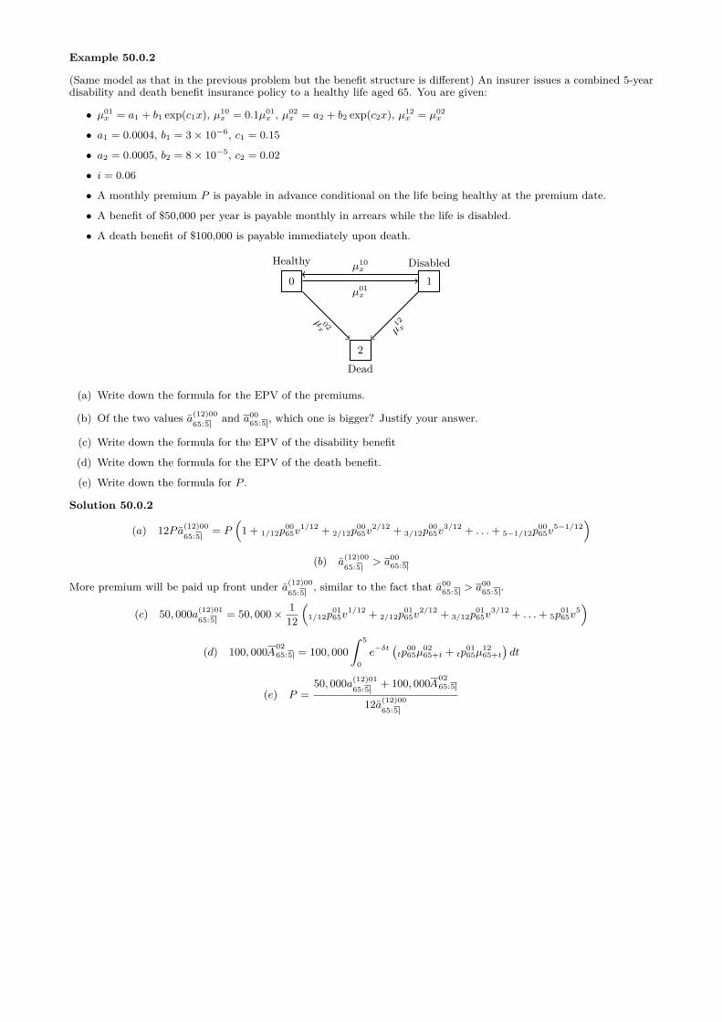
Example 50.0.2
(Same model as that in the previous problem but the benefit structure is different) An insurer issues a combined 5-yeardisability and death benefit insurance policy to a healthy life aged 65. You are given:
• µ01x = a1 + b1 exp(c1x), µ10
x = 0.1µ01x , µ02
x = a2 + b2 exp(c2x), µ12x = µ02
x
• a1 = 0.0004, b1 = 3× 10⁻⁶, c1 = 0.15
• a2 = 0.0005, b2 = 8× 10⁻⁵, c2 = 0.02
• i = 0.06
• A monthly premium P is payable in advance conditional on the life being healthy at the premium date.
• A benefit of $50,000 per year is payable monthly in arrears while the life is disabled.
• A death benefit of $100,000 is payable immediately upon death.
Healthy Disabled
Dead
0 1
2
µ10x
µ01x
µ 02x µ12x
(a) Write down the formula for the EPV of the premiums.
(b) Of the two values a(12)0065:5 and a00
65:5 , which one is bigger? Justify your answer.
(c) Write down the formula for the EPV of the disability benefit
(d) Write down the formula for the EPV of the death benefit.
(e) Write down the formula for P .
Solution 50.0.2
(a) 12P a(12)0065:5 = P
(1 + 1/12p
0065v
1/12 + 2/12p0065v
2/12 + 3/12p0065v
3/12 + . . .+ 5−1/12p0065v
5−1/12)
(b) a(12)0065:5 > a00
65:5
More premium will be paid up front under a(12)0065:5 , similar to the fact that a00
65:5 > a0065:5 .
(c) 50, 000a(12)0165:5 = 50, 000× 1
12
(1/12p
0165v
1/12 + 2/12p0165v
2/12 + 3/12p0165v
3/12 + . . .+ 5p0165v
5)
(d) 100, 000A0265:5 = 100, 000
∫ 5
0e−δt
(tp
0065µ
0265+t + tp
0165µ
1265+t
)dt
(e) P =50, 000a(12)01
65:5 + 100, 000A0265:5
12a(12)0065:5

50.1 Check your knowledge
Homework 50.1.1
An insurer issues a combined 10-year disability and death benefit policy to a healthy life aged 50. You are given:
Healthy Disabled
Dead
0 1
2
µ10x+t
µ01x+t
µ 02x+t µ
12x+t
(a) The product pays a continuous disability benefit at the rate of 50,000 per year while the insured is disabled, andpays a death benefit of 100,000 at the moment of death.
(b) Gross premium is payable continuously at the rate of P per year while the insured is healthy
(c) Premium expense is 2% of the gross premium. There are no other expenses.
(d) δ = 0.05
(e) µ01x+t = 0.02, µ10
x+t = 0.01, µ02x+t = 0.01 + 0.005t, µ12
x+t = 0.02 + 0.01t
Selective actuarial values where x = 50 and n = 10:
k A01x+k:n−k A
02x+k:n−k A
12x+k:n−k a00
x+k:n−k a01x+k:n−k a10
x+k:n−k a11x+k:n−k
0 0.12856 0.23701 0.37223 6.49636 0.50610 0.26205 6.146855 0.07652 0.19262 0.32982 3.84198 0.16607 0.08384 3.61567
(a) Calculate P .
(b) Actuary Mark decided to invent a new symbolAi→j→rx:n to represent the APV of the benefit 1 payable immediately
up on (x) moving from the state j to the state r during the first n years given that the insured is in the state i attime zero. Calculate the sum of A0→0→2
55:5 and A0→1→255:5 for this policy.
(c) Actuary Katie is a computation wizard and can calculate anything including a0250+k:10−k and a12
50+k:10−k where0 ≤ k ≤ 10. Define these two symbols and explain whether it ever makes sense for her to calculate these two valuesfor this policy.
(d) This is how Actuary Jeff explains the difference between a0250:10 and a12
50:10 : Both symbols represent the APV ofthe benefit 1 payable continuously while the insured is dead, with payments ceasing after first 10 years. However,a02
50:10 is the APV of such benefits where the insured is healthy at death. In contrast, a1250:10 is the APV of such
benefits where the insured is disabled at death. Is Jeff’s explanation correct?
(e) Define the symbol A0250+k:10−k .
(f) Calculate the gross premium policy value 5V(0).
(g) Calculate the gross premium policy value 5V(1).
(h) Calculate the gross premium policy value 5V(2).
(i) Use the Euler’s method and calculate the gross premium policy value two months before policy expiration giventhat the insured is healthy at that time.
(j) Use the Euler’s method and calculate the gross premium policy value two months before policy expiration giventhat the insured is disabled at that time.
Homework Solution 50.1.1
Difficulty
(a) P =50, 000a01
50:10 + 100, 000A0250:10
0.98a0050:10
= 50, 000× 0.50610 + 100, 000× 0.237010.98× 6.49636 = 7, 697.62
(b) A0→0→255:5 +A
0→1→255:5 =A
0255:5 = 0.19262
(c) a0250+k:10−k =
∫ 10−k
0e−δttp
0250+kdt, a12
50+k:10−k =∫ 10−k
0e−δttp
1250+kdt
These two values will be useful if a benefit is paid continuously while the insured is dead given that the insured iscurrently healthy or disabled. Since no insurer will design such a policy, these two values will never be used in any usefulactuarial calculations.
407 c© Yufeng Guo, MLC Fall 2017

(d) Jeff’s explanation is wrong. a0250:10 includes the path 0→ 2 and the path 0→ 1→ 2. For a payment to be made, the
insured needs to be healthy at time zero and be dead at any time during the first ten years. The insured can be healthyor disabled at death.
Similarly, a1250:10 includes the path 1→ 2 and the path 1→ 0→ 2.
(e) A0250+k:10−k =
∫ 10−k
0
∑j 6=2
e−δt tp0j50+t µ
j250+kdt =
∫ 10−k
0e−δt tp
0050+t µ
0250+kdt+
∫ 10−k
0e−δt tp
0150+t µ
1250+kdt
(f) 5V(0) = 50, 000a01
55:5 + 100, 000A0255:5 − 0.98Pa00
55:5= 50, 000× 0.16607 + 100, 000× 0.192617− 0.98× 7, 697.56× 3.84198 = 1, 417
(g) 5V(1) = 50, 000a11
55:5 + 100, 000A1255:5 − 0.98Pa10
55:5= 50, 000× 3.61567 + 100, 000× 0.32982− 0.98× 7, 697.56× 0.083841 = 213, 133
(h) 5V(2) = 0 because the future payment is zero given that the insured is in the state 2
(i), (j)for 0 ≤ t ≤ 10
d
dttV
(0) = tV(0)δ + 0.98P − µ01
50+t
(tV
(1) − tV(0))− µ02
50+t
(100, 000− tV
(0))
d
dttV
(1) = tV(1)δ − 50, 000− µ10
50+t
(tV
(0) − tV(1))− µ12
50+t
(100, 000− tV
(1))
10V(0) = 10V
(1) = 0(d
dttV
(0))t=10
= 0δ + 0.98P − µ0150+10(0− 0)− µ02
50+10(100, 000− 0)
= 0.98P − µ0250+10100, 000 = 0.98× 7, 697.56− (0.01 + 0.005× 10)100, 000 = 1543.6088(
d
dttV
(0))t=10
≈ 10V(0) − 10−1/12V
(0)
1/12 =0− 10−1/12V
(0)
1/12 = 1543.6088
⇒ 10−1/12V(0) ≈ −128.64(
d
dttV
(1))t=10
= 0δ − 50, 000− µ1050+10(0− 0)− µ12
50+10(100, 000− 0)
= −50, 000− (0.02 + 0.01× 10)100, 000 = −62, 000.00(d
dttV
(1))t=10
≈ 10V(1) − 10−1/12V
(1)
1/12 =0− 10−1/12V
(1)
1/12 = −62, 000.00
⇒ 10−1/12V(1) ≈ 5, 166.67(
d
dttV
(0))t=10−1/12
= 10−1/12V(0)δ + 0.98P − µ01
50+10−1/12
(10−1/12V
(1) − 10−1/12V(0))− µ02
50+10−1/12
(100, 000− 10−1/12V
(0))
= −128.64× 0.0 + 0.98× 7, 697.56− 0.02(5, 166.67−−128.64)−(0.01 + 0.005(10− 1/12)
)(100, 000−−128.64)
= 1, 465.34(d
dttV
(0))t=10−1/12
≈ 10−1/12V(0) − 10−2/12V
(0)
1/12 =−128.64− 10−2/12V
(0)
1/12 = 1, 465.34
⇒ 10−2/12V(0) ≈ −250.75(
d
dttV
(1))t=10−1/12
= 10−1/12V(1)δ − 50, 000− µ10
50+10−1/12
(10−1/12V
(0) − 10−1/12V(1))− µ12
50+10−1/12
(100, 000− 10−1/12V
(1))
= 5, 166.67× 0.05− 50, 000− 0.01(−128.64− 5, 166.67)−(0.02 + 0.01(10− 1/12)
)(100, 000− 5, 166.67)
= −60, 989.69(d
dttV
(1))t=10−1/12
≈ 10−1/12V(1) − 10−2/12V
(1)
1/12 =5, 166.67− 10−2/12V
(1)
1/12 = −60, 989.69
⇒ 10−2/12V(1) ≈ 10, 249.14

Homework 50.1.2
An insurer issues a combined 5-year disability and death benefit policy to a healthy life aged 60. You are given:
Healthy Disabled
Dead
0 1
2
µ10x+t
µ01x+t
µ 02x+t µ
12x+t
(a) Disability benefit: payable continuously at the rate of 75,000 per year while the insured is disabled
(b) Death benefit: 100,000 at the moment of death if the insured is healthy at death and 25,000 at the moment ofdeath if the insured is disabled at death
(c) Gross premium: payable continuously at the rate of P per year while the insured is healthy
(d) Premium expenses: 5% of the premium incurred continuously.
(e) Death claim cost: 200 per claim.
(f) Maintenance expense while the insured is disabled: at the rate of 300 per year incurred continuously
(g) δ = 0.06
(h) µ01x+t = 0.04, µ02
x+t = 0.01 + 0.02t, µ10x+t = 0.02, µ12
x+t = 0.02 + 0.02t
Selective actuarial values where x = 60 and n = 5:
k A01x+k:n−k A
02x+k:n−k A
12x+k:n−k a00
x+k:n−k a01x+k:n−k a10
x+k:n−k a11x+k:n−k
∫ 5−k0 e−δttp
01x+kµ
12x+k+tdt
0 0.14257 0.21562 0.24328 3.62381 0.32389 0.16194 3.74268 0.025643 0.06723 0.15422 0.16911 1.68923 0.06616 0.03308 1.76286 0.00644
You are also given:∫ 2
0 e−δt
tp1163µ
1263+tdt = 0.16620
(a) Show that P = 12, 800 to the nearest of 50.
(b) Show that 3V(0) = −600 to the nearest of 10.
(c) Calculate 3V(1).
(d) Calculate 3V(2).
(e) Write down the Thiele’s differential equation for tV (0) and for tV (1) and the associated boundary conditions.
(f) Use the Euler’s method and derive the backwards recursive formula for t−hV(0) as a function of tV (0); derive the
backwards recursive formula for t−hV (1) as a function of tV (1).
(g) Use the backwards recursive formulas derived above and calculate 5−2/12V(0) and 5−2/12V
(1) (e.g. the policy valuestwo months before policy expiration).
Homework Solution 50.1.2
Difficulty
(a) P = PVFB0.95a00
60:5
PVFB = 75, 300a0160:5 + 100, 200
∫ 5
0e−δttp
0060µ
0260+tdt+ 25, 200
∫ 5
0e−δttp
0160µ
1260+tdt
= 75, 300a0160:5 + 100, 200
(∫ 5
0e−δttp
0060µ
0260+tdt+
∫ 5
0e−δttp
0160µ
1260+tdt
)− 75, 000
∫ 5
0e−δttp
0160µ
1260+tdt
= 75, 300a0160:5 + 100, 200A02
60:5 − 75, 000∫ 5
0e−δttp
0160µ
1260+tdt
= 75, 300× 0.32389 + 100, 200× 0.21562− 75, 000× 0.02564 = 44, 071
P = 44, 0710.95a00
60:5= 44, 071
0.95× 3.62381 = 12, 802
409 c© Yufeng Guo, MLC Fall 2017
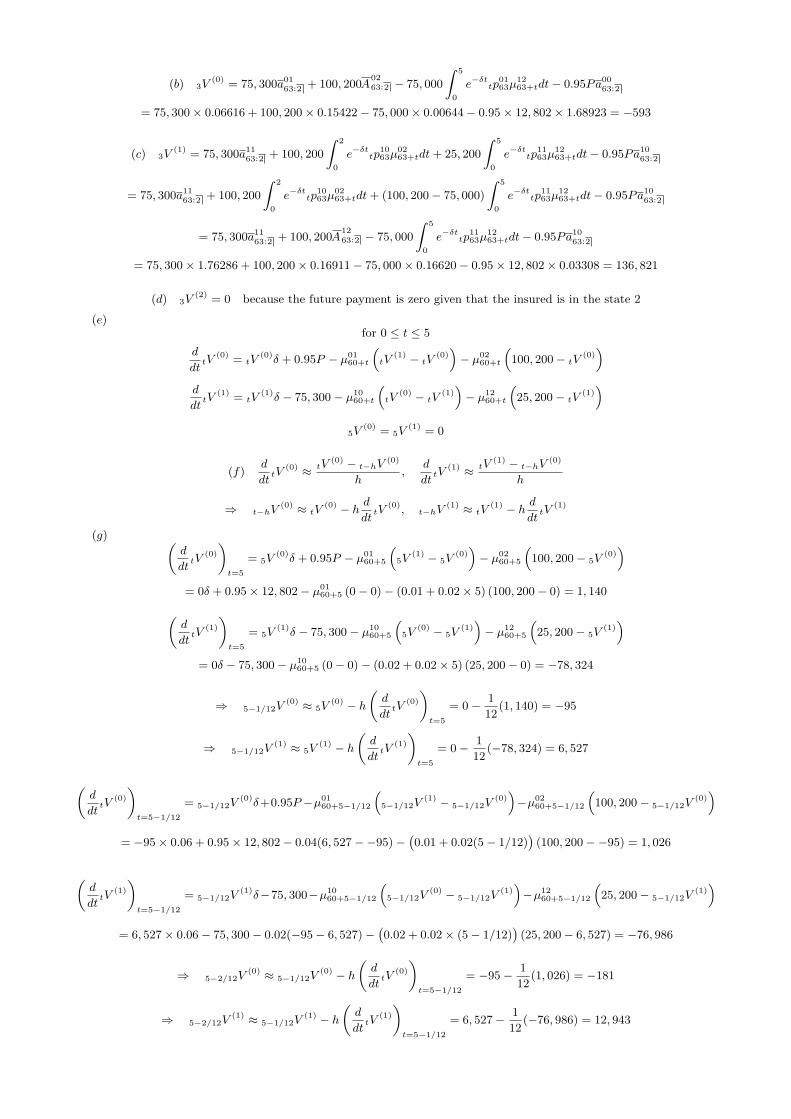
(b) 3V(0) = 75, 300a01
63:2 + 100, 200A0263:2 − 75, 000
∫ 5
0e−δttp
0163µ
1263+tdt− 0.95Pa00
63:2
= 75, 300× 0.06616 + 100, 200× 0.15422− 75, 000× 0.00644− 0.95× 12, 802× 1.68923 = −593
(c) 3V(1) = 75, 300a11
63:2 + 100, 200∫ 2
0e−δttp
1063µ
0263+tdt+ 25, 200
∫ 5
0e−δttp
1163µ
1263+tdt− 0.95Pa10
63:2
= 75, 300a1163:2 + 100, 200
∫ 2
0e−δttp
1063µ
0263+tdt+ (100, 200− 75, 000)
∫ 5
0e−δttp
1163µ
1263+tdt− 0.95Pa10
63:2
= 75, 300a1163:2 + 100, 200A12
63:2 − 75, 000∫ 5
0e−δttp
1163µ
1263+tdt− 0.95Pa10
63:2
= 75, 300× 1.76286 + 100, 200× 0.16911− 75, 000× 0.16620− 0.95× 12, 802× 0.03308 = 136, 821
(d) 3V(2) = 0 because the future payment is zero given that the insured is in the state 2
(e)for 0 ≤ t ≤ 5
d
dttV
(0) = tV(0)δ + 0.95P − µ01
60+t
(tV
(1) − tV(0))− µ02
60+t
(100, 200− tV
(0))
d
dttV
(1) = tV(1)δ − 75, 300− µ10
60+t
(tV
(0) − tV(1))− µ12
60+t
(25, 200− tV
(1))
5V(0) = 5V
(1) = 0
(f) d
dttV
(0) ≈ tV(0) − t−hV
(0)
h,
d
dttV
(1) ≈ tV(1) − t−hV
(0)
h
⇒ t−hV(0) ≈ tV
(0) − h ddttV
(0), t−hV(1) ≈ tV
(1) − h ddttV
(1)
(g) (d
dttV
(0))t=5
= 5V(0)δ + 0.95P − µ01
60+5
(5V
(1) − 5V(0))− µ02
60+5
(100, 200− 5V
(0))
= 0δ + 0.95× 12, 802− µ0160+5 (0− 0)− (0.01 + 0.02× 5) (100, 200− 0) = 1, 140(
d
dttV
(1))t=5
= 5V(1)δ − 75, 300− µ10
60+5
(5V
(0) − 5V(1))− µ12
60+5
(25, 200− 5V
(1))
= 0δ − 75, 300− µ1060+5 (0− 0)− (0.02 + 0.02× 5) (25, 200− 0) = −78, 324
⇒ 5−1/12V(0) ≈ 5V
(0) − h(d
dttV
(0))t=5
= 0− 112(1, 140) = −95
⇒ 5−1/12V(1) ≈ 5V
(1) − h(d
dttV
(1))t=5
= 0− 112(−78, 324) = 6, 527
(d
dttV
(0))t=5−1/12
= 5−1/12V(0)δ+0.95P−µ01
60+5−1/12
(5−1/12V
(1) − 5−1/12V(0))−µ02
60+5−1/12
(100, 200− 5−1/12V
(0))
= −95× 0.06 + 0.95× 12, 802− 0.04(6, 527−−95)−(0.01 + 0.02(5− 1/12)
)(100, 200−−95) = 1, 026
(d
dttV
(1))t=5−1/12
= 5−1/12V(1)δ−75, 300−µ10
60+5−1/12
(5−1/12V
(0) − 5−1/12V(1))−µ12
60+5−1/12
(25, 200− 5−1/12V
(1))
= 6, 527× 0.06− 75, 300− 0.02(−95− 6, 527)−(0.02 + 0.02× (5− 1/12)
)(25, 200− 6, 527) = −76, 986
⇒ 5−2/12V(0) ≈ 5−1/12V
(0) − h(d
dttV
(0))t=5−1/12
= −95− 112(1, 026) = −181
⇒ 5−2/12V(1) ≈ 5−1/12V
(1) − h(d
dttV
(1))t=5−1/12
= 6, 527− 112(−76, 986) = 12, 943

Homework 50.1.3
(Model parameters are from the AMLCR Exercise 8.7) A combined 10-year term disability income, critical illness benefit,and death benefit policy is issued to a healthy life age 60.
Healthy Sick
Dead Critically ill
0 1
2 3
µ01x+t
µ10x+t
µ02x+t
µ13x+t
µ32x+t
µ12x+tµ03
x+t
Healthy Sick
Dead Critically ill
0 1
2 3
150,000
50,000
50,000
50,000
100,000100,000
You are given:
• µ01x = a1 + b1 exp{c1x}, µ02
x = a2 + b2 exp{c2x}
• µ12x = µ02
x , µ32x = 1.2µ02
x
• µ10x = 0.1µ01
x , µ03x = 0.05µ01
x , µ13x = µ03
x
• a1 = 4× 10⁻⁴, b1 = 3.5× 10⁻⁶, c1 = 0.14
• a2 = 5× 10⁻⁴, b2 = 7.6× 10⁻⁵, c2 = 0.09
• δ = 6%
• Net premium: payable continuously at the rate of Pper year while the insured is healthy.
Benefits:
• Death benefit payable immediately upon death:150,000 if the insured is healthy at death, 100,000 ifthe insured is disabled (e.g. sick) at death, and 50,000if the insured is critically ill at death.
• Disability benefit: 50,000 per year payable continu-ously where the insured is disabled.
• Critical illness benefit payable immediately upon be-coming critically ill: 100,000 if the insured is healthybefore turning critically ill and 50,000 if the insured issick before turning critically ill.
Selective actuarial values for x = 60 and n = 10:
k A01x+k:n−k A
02x+k:n−k A
03x+k:n−k A
12x+k:n−k a00
x+k:n−k a01x+k:n−k a10
x+k:n−k a11x+k:n−k
0 0.19161 0.18605 0.01105 0.18457 6.39703 0.72502 0.07250 7.07677
k∫ n−k
0 e−δttp01x µ
12x+tdt
∫ n−k0 e−δttp
01x µ
13x+tdt
∫ n−k0 e−δttp
03x µ
32x+tdt
0 0.02235 0.00147 0.00148
(a) Show that P = 10, 000 to the nearest of 10.
(b) Derive the formula for tV (0) where 0 < t < 10.
(c) Derive the formula for tV (1) where 0 < t < 10.
(d) Derive the formula for tV (3) where 0 < t < 10.
(e) Use general reasoning to derive the formula for d
dttV
(0) and d
dttV
(1) where 0 < t < 10. Rigorous proof is notexpected.
(f) Estimate the net premium P . You are given:
• 0V(0) = 1, 585.94 if P = 9, 800
• 0V(0) = −327.15 if P = 10, 100
(g) Re-do Part (e) assuming that the insurer charges a single net premium at issue.
Homework Solution 50.1.3
Difficulty(a)
PVFB death = 150, 000∫ 10
0e−δttp
0060µ
0260+tdt+ 100, 000
∫ 10
0e−δttp
0160µ
1260+tdt+ 50, 000
∫ 10
0e−δttp
0360µ
3260+tdt
A0260:5 =
∫ 10
0e−δttp
0060µ
0260+tdt+
∫ 10
0e−δttp
0160µ
1260+tdt+
∫ 10
0e−δttp
0360µ
3260+tdt = 0.18605∫ 10
0e−δttp
0160µ
1260+tdt = 0.02235,
∫ 10
0e−δttp
0360µ
3260+tdt = 0.00148
PVFB death = 150, 000× 0.18605− 50, 000× 0.02235− 100, 000× 0.00148 = 26, 642
411 c© Yufeng Guo, MLC Fall 2017
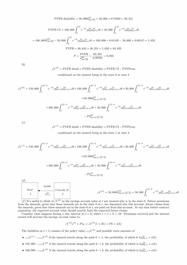
PVFB disability = 50, 000a0160:10 = 50, 000× 0.72502 = 36, 251
PVFB CI = 100, 000∫ 10
0e−δttp
0060µ
0360+tdt+ 50, 000
∫ 10
0e−δttp
0160µ
1360+tdt
= 100, 000A0360:10 − 50, 000
∫ 10
0e−δttp
0160µ
1360+tdt = 100, 000× 0.01105− 50, 000× 0.00147 = 1, 032
PVFB = 26, 642 + 36, 251 + 1, 032 = 63, 925
P = PVFBa00
60:10= 63, 925
6.39703 = 9, 993
(b)kV
(0) = PVFB death + PVFB disability + PVFB CI− PVFPrem
conditional on the insured being in the state 0 at time k
kV(0) = 150, 000
∫ 10−k
0e−δttp
0060+kµ
0260+k+tdt+100, 000
∫ 10−k
0e−δttp
0160+kµ
1260+k+tdt+50, 000
∫ 10−k
0e−δttp
0360+kµ
3260+k+tdt
+50, 000a0160+k:10−k
+100, 000∫ 10−k
0e−δttp
0060+kµ
0360+k+tdt+ 50, 000
∫ 10−k
0e−δttp
0160+kµ
1360+k+tdt
−Pa0060+k:10−k
(c)kV
(1) = PVFB death + PVFB disability + PVFB CI− PVFPrem
conditional on the insured being in the state 1 at time k
kV(1) = 150, 000
∫ 10−k
0e−δttp
1060+kµ
0260+k+tdt+100, 000
∫ 10−k
0e−δttp
1160+kµ
1260+k+tdt+50, 000
∫ 10−k
0e−δttp
1360+kµ
3260+k+tdt
+50, 000a1160+k:10−k
+100, 000∫ 10−k
0e−δttp
1060+kµ
0360+k+tdt+ 50, 000
∫ 10−k
0e−δttp
1160+kµ
1360+k+tdt
−Pa1060+k:10−k
(d)
Dead Critically ill
2 3µ32x+t
50,000
kV(3) = 50, 000A32
60+k:10−k = 50, 000∫ 10−k
0e−δttp
3360+kµ
3260+k+tdt
(f) It’s useful to think of tV (0) as the savings account value at t per insured who is in the state 0. Future premiumsfrom the insureds, given that these insureds are in the state 0 at t, are deposited into this account; future claims fromthe insureds, given that these insureds are in the state 0 at t, are paid out from this account. At any time before contractexpiration, the expected account value should exactly fund the expected future claims.
Consider what happens during a tiny interval [h, t + h] where t < t + h < 10. Premiums received and the interestearned will increase the savings account value to:
tV(0)eδh + Psh = tV
(0)(1 + δh) + Ph+ o(h)
The liabilities at t+ h consists of the policy value t+hV(0) and possible extra amounts of
• t+hV(1) − t+hV
(0) if the insured travels along the path 0→ 1, the probability of which is hµ0160+t + o(h)
• 150, 000− t+hV(0) if the insured travels along the path 0→ 2, the probability of which is hµ02
60+t + o(h)
• 100, 000− t+hV(0) if the insured travels along the path 0→ 3, the probability of which is hµ03
60+t + o(h)

tV(0)(1+δh)+Ph = t+hV
(0)+hµ0160+t
(t+hV
(1) − t+hV(0))
+hµ0260+t
(150, 000− t+hV
(0))
+hµ0360+t
(100, 000− t+hV
(0))
+o(h)
Rearrange the above formula, divide by h, and let h→ 0:
d
dttV
(0) = tV(0)δ + P − µ01
60+t
(tV
(1) − tV(0))− µ02
60+t
(150, 000− tV
(0))− µ03
60+t
(100, 000− tV
(0))
Follow the same reasoning:
d
dttV
(1) = tV(1)δ − 50, 000− µ10
60+t
(tV
(0) − tV(1))− µ12
60+t
(100, 000− tV
(1))− µ13
60+t
(50, 000− tV
(1))
(e) We’ll use linear interpolation to find P such that 0V(0) = 0.
P ≈ 9, 800 + 0− 1, 585.94−327.15− 1, 585.94 × (10, 100− 9, 800) = 10, 049
This is different from the premium in Part (a) because the two methods are different.
(f)d
dttV
(0) = tV(0)δ − µ01
60+t
(tV
(1) − tV(0))− µ02
60+t
(150, 000− tV
(0))− µ03
60+t
(100, 000− tV
(0))
The formula for d
dttV
(1) remains the same.
413 c© Yufeng Guo, MLC Fall 2017


Chapter 51
Multiple state: age retirement, disability, withdrawal
Example 51.0.1
You are given the following multiple state model:
dead in
service
4
withdrawn disability
retirement
age
retirement
member
0
1 2 3
(i)
µ01x =
0.08 for 40 ≤ x < 500.04 for 50 ≤ x < 600.00 for x ≥ 60
(ii) µ02x = 0.002
(iii)
µ03x =
{0.0 for x < 600.1 for 60 ≤ x < 65
(iv) 20% of the members surviving in employ-ment to age 60 retire at that time.
(v) 100% of the members surviving in employ-ment to age 65 retire at that time.
(vi) µ04x = 0.005
(a) For each mode of exit, calculate the probability that a member aged 40 exits employment by that mode.
(b) Calculate the probability that a member aged 40 will retire at age 65.
Solution 51.0.1
µ0140+t µ02
40+t µ0340+t µ04
40+t Total tp0040
0 ≤ t < 10 0.08 0.002 0.0 0.005 0.087 e−0.087t
10 ≤ t < 20 0.04 0.002 0.0 0.005 0.047 e−0.087×10e−0.047(t−10)
t = 20+ e−0.087×10e−0.047×100.820+ < t < 25 0.00 0.002 0.1 0.005 0.107 e−0.087×10e−0.047×100.8e−0.107(t−20)
(a)
P (exit by force j by age 50) = 10p0j40 =
∫ 10
0tp
0040µ
0j40+tdt =
∫ 10
0e−0.087tµ0j
40+tdt =µ0j
40+t
0.087(1− e−0.087×10)
P (exit by force j after age 50 and before age 60) =∫ 20
10tp
0040µ
0j40+tdt =
∫ 20
10e−0.087×10e−0.047(t−10)µ0j
40+tdt
= e−0.087×10∫ 10
0e−0.047tµ0j
40+10+tdt = e−0.087×10 µ0j40+10+t
0.047(1− e−0.047×10)
P (exit by force j after age 60 and before age 65) =∫ 25
20+tp
0040µ
0240+tdt
=∫ 25
20+e−0.087×10e−0.047×100.8e−0.107(t−20)µ0j
40+tdt =∫ 5
0e−0.087×10e−0.047×100.8e−0.107tµ0j
40+20+tdt
= e−0.087×10e−0.047×10 × 0.8×µ0j
40+20+t
0.107(1− e−0.107×5)
P (exit by force 1) = 0.080.087
(1− e−0.087×10)+e−0.087×10 0.04
0.047(1− e−0.047×10)+e−0.087×10e−0.047×10×0.8× 0
0.107(1− e−0.107×5)
= 0.66800456
415

P (exit by force 2) = 0.0020.087
(1− e−0.087×10)+e−0.087×10 0.002
0.047(1− e−0.047×10)+e−0.087×10e−0.047×10×0.8×0.002
0.107(1− e−0.107×5)
= 0.02166508
P (exit by force 4) = 0.0050.087
(1− e−0.087×10)+e−0.087×10 0.005
0.047(1− e−0.047×10)+e−0.087×10e−0.047×10×0.8×0.005
0.107(1− e−0.107×5)
= 52 × P (exit by force 4) = 0.05416271
P (exit by force 3 excluding point decrement at age 60 and age 65)
= 00.087
(1− e−0.087×10)+ e−0.087×10 0
0.047(1− e−0.047×10)+ e−0.087×10e−0.047×10 × 0.8× 0.1
0.107(1− e−0.107×5)
= 0.08111454
P (retire at age 60) = 0.220−p0040 = e−0.087×10e−0.047×10 = 0.05236913
P (retire at age 65) = 25+p0040 = e−0.087×10e−0.047×100.8e−0.107×5 = 0.12268397
⇒ P (exit by age retirement) = 0.08111454 + 0.05236913 + 0.12268397 = 0.25616764
check total:0.66800456 + 0.02166508 + 0.05416271 + 0.25616764 = 0.99999999 ≈ 1 OK
(b) 25−p0040 = e−0.087×10e−0.047×100.8e−0.107(25−20) = 0.12268397
51.1 Check your knowledge
Homework 51.1.1
You are given the following multiple state model:
dead in
service
4
withdrawn disability
retirement
age
retirement
member
0
1 2 3
(i)
µ01x =
0.06 for 30 ≤ x < 450.02 for 45 ≤ x < 600.00 for x ≥ 60
µ02x =
0.002 for 30 ≤ x < 450.004 for 45 ≤ x < 600.006 for x ≥ 60
(ii)
µ03x =
{0.0 for x < 600.2 for 60 ≤ x < 65
(iii) 40% of the members surviving in employ-ment to age 60 retire at that time.
(iv) 100% of the members surviving in employ-ment to age 65 retire at that time.
(v)
µ04x =
{0.005 for x < 600.010 for 60 ≤ x < 65
(a) For each mode of exit, calculate the probability that a member aged 30 exits employment by that mode.
(b) Calculate the probability that a member aged 30 will retire at age 65.
Homework Solution 51.1.1
Difficulty
µ0130+t µ02
30+t µ0330+t µ04
30+t Total tp0030
0 ≤ t < 15 0.06 0.002 0.0 0.005 0.067 e−0.067t
15 ≤ t < 30 0.02 0.004 0.0 0.005 0.029 e−0.067×15e−0.029(t−15)
t = 30+ e−0.067×15e−0.029×150.630+ < t < 35 0.00 0.006 0.2 0.010 0.216 e−0.067×15e−0.029×150.6e−0.216(t−30)
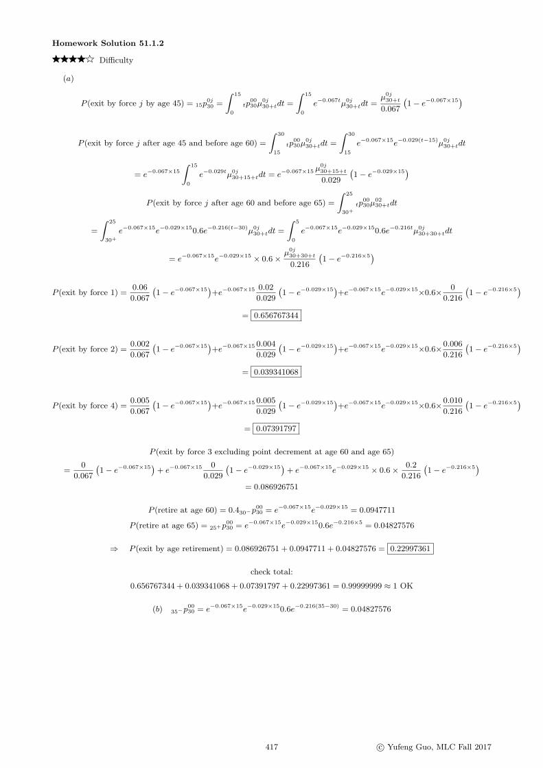
Homework Solution 51.1.2
Difficulty
(a)
P (exit by force j by age 45) = 15p0j30 =
∫ 15
0tp
0030µ
0j30+tdt =
∫ 15
0e−0.067tµ0j
30+tdt =µ0j
30+t
0.067(1− e−0.067×15)
P (exit by force j after age 45 and before age 60) =∫ 30
15tp
0030µ
0j30+tdt =
∫ 30
15e−0.067×15e−0.029(t−15)µ0j
30+tdt
= e−0.067×15∫ 15
0e−0.029tµ0j
30+15+tdt = e−0.067×15 µ0j30+15+t
0.029(1− e−0.029×15)
P (exit by force j after age 60 and before age 65) =∫ 25
30+tp
0030µ
0230+tdt
=∫ 25
30+e−0.067×15e−0.029×150.6e−0.216(t−30)µ0j
30+tdt =∫ 5
0e−0.067×15e−0.029×150.6e−0.216tµ0j
30+30+tdt
= e−0.067×15e−0.029×15 × 0.6×µ0j
30+30+t
0.216(1− e−0.216×5)
P (exit by force 1) = 0.060.067
(1− e−0.067×15)+e−0.067×15 0.02
0.029(1− e−0.029×15)+e−0.067×15e−0.029×15×0.6× 0
0.216(1− e−0.216×5)
= 0.656767344
P (exit by force 2) = 0.0020.067
(1− e−0.067×15)+e−0.067×15 0.004
0.029(1− e−0.029×15)+e−0.067×15e−0.029×15×0.6×0.006
0.216(1− e−0.216×5)
= 0.039341068
P (exit by force 4) = 0.0050.067
(1− e−0.067×15)+e−0.067×15 0.005
0.029(1− e−0.029×15)+e−0.067×15e−0.029×15×0.6×0.010
0.216(1− e−0.216×5)
= 0.07391797
P (exit by force 3 excluding point decrement at age 60 and age 65)
= 00.067
(1− e−0.067×15)+ e−0.067×15 0
0.029(1− e−0.029×15)+ e−0.067×15e−0.029×15 × 0.6× 0.2
0.216(1− e−0.216×5)
= 0.086926751
P (retire at age 60) = 0.430−p0030 = e−0.067×15e−0.029×15 = 0.0947711
P (retire at age 65) = 25+p0030 = e−0.067×15e−0.029×150.6e−0.216×5 = 0.04827576
⇒ P (exit by age retirement) = 0.086926751 + 0.0947711 + 0.04827576 = 0.22997361
check total:0.656767344 + 0.039341068 + 0.07391797 + 0.22997361 = 0.99999999 ≈ 1 OK
(b) 35−p0030 = e−0.067×15e−0.029×150.6e−0.216(35−30) = 0.04827576
417 c© Yufeng Guo, MLC Fall 2017
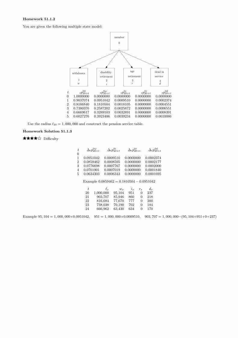
Homework 51.1.2
You are given the following multiple state model:
dead in
service
4
withdrawn disability
retirement
age
retirement
member
0
1 2 3w i r d
t tp0020+t tp
0w20+t tp
0i20+t tp
0r20+t tp
0d20+t
0 1.0000000 0.0000000 0.0000000 0.0000000 0.00000001 0.9037074 0.0951042 0.0009510 0.0000000 0.00023742 0.8166840 0.1810504 0.0018105 0.0000000 0.00045513 0.7380376 0.2587202 0.0025872 0.0000000 0.00065514 0.6669617 0.3289103 0.0032891 0.0000000 0.00083915 0.6027276 0.3923406 0.0039234 0.0000000 0.0010086
Use the radius `20 = 1, 000, 000 and construct the pension service table.
Homework Solution 51.1.3
Difficulty
t ∆tp0w20+t ∆tp
0i20+t ∆tp
0r20+t ∆tp
0d20+t
01 0.0951042 0.0009510 0.0000000 0.00023742 0.0859462 0.0008595 0.0000000 0.00021773 0.0776698 0.0007767 0.0000000 0.00020004 0.0701901 0.0007019 0.0000000 0.00018405 0.0634303 0.0006343 0.0000000 0.0001695
Example 0.0859462 = 0.1810504− 0.0951042
t `x wx ix rx dx20 1,000,000 95,104 951 0 23721 903,707 85,946 860 0 21822 816,684 77,670 777 0 20023 738,038 70,190 702 0 18424 666,962 63,430 634 0 170
Example 95, 104 = 1, 000, 000×0.0951042, 951 = 1, 000, 000×0.0009510, 903, 707 = 1, 000, 000−(95, 104+951+0+237)

Homework 51.1.3
You are given the following withdrawal/retirement model:
Retired
Employee
0
Withdrawn
2
Dead
3
1
You are also given:
(i) The force of mortality depends on the individual’s age only and follows the Illustrative Life Table. That is,µ03x = µ13
x = µ23x = µx, where µx is equal to the force of mortality in the Illustrative Life Table (ILT).
(ii)
µ02x =
{0.002 if x < 600.000 if x ≥ 60
(iii) Employees retire exactly on age 60, 61, 62, 63, 64, or 65.
(iv) 20% of the employees reaching age 60, 61, 62, 63, and 64 retire at that age; 100% of the employees reaching age65 retire at the age.
(v) Death benefit after retirement: 1 at the end of the year of death.
(vi) i = 0.06.
For an employee currently aged 50, derive the EPV of the post-retirement death benefit. Numerical calculations arenot expected.
Homework Solution 51.1.4
Difficulty(a) Sample calculation:
EPV of death benefit for those who retire at age 65= P (not withdraw from age 50 to 60)×P (not die from age 50 to 65)
×P (not retire at age 60 or 61 or 62 or 63 or 64)×P (retire from age 65)
×v15
×EPV of whole life insurance of 1 on 65 in ILT= e−0.002×10
15p50 × 0.85 × 1× v15A65 = e−0.002×10 × 0.85 × 1× 15E50A65
EPV of post retirement death benefit
= e−0.002×10(
0.2(
10E50A60 + 0.811E50A61 + 0.8212E60A62 + 0.83
13E60A63 + 0.8414E60A64
)+ 0.85
15E60A65
)
419 c© Yufeng Guo, MLC Fall 2017

Homework 51.1.4
You are given the following withdrawal/retirement model:
Retired
Employee
0
Withdrawn
2
Dead
3
1
You are also given:
(i) The force of mortality depends on the individual’s age only and follows the Illustrative Life Table (ILT). That is,µ03x = µ13
x = µ23x = µx, where µx is equal to the force of mortality in the Illustrative Life Table. In addition, deaths
are uniformly distributed over each year of age.
(ii)
µ02x =
{0.001 if x < 600.000 if x ≥ 60
(iii) Employees retire exactly on age 60, 62, 64, or 65.
(iv) 30% of the employees reaching age 60, 62, and 64 retire at that age; 100% of the employees reaching age 65 retireat the age.
(v) Death benefit after retirement: 100,000 at the moment of death.
(vi) i = 0.06.
(vii) Selective actuarial values:
k kE55 A55+k5 0.708101 0.369136 0.658828 0.382797 0.612206 0.396708 0.568091 0.410859 0.526352 0.4252210 0.486864 0.43980
(a) Show that the probability that an employee aged x is dead by age x + t is the same as that under the alive-deadmodel with the transition intensity µx.
(b) For an employee currently aged 55, show that the EPV of the post-retirement death benefit is 24,200 to the nearestof 50.
Homework Solution 51.1.5
Difficulty(a)
d
dttp
03x = tp
00x µ
03x+t + tp
01x µ
13x+t + tp
02x µ
23x+t
=(tp
00x + tp
01x + tp
02x
)µx+t =
(1− tp
03x
)µx+t
boundary conditions: 0p00x = 1, 0p
03x = 0
Now consider the following the alive-death model:
Employee
0
Dead
3
µx
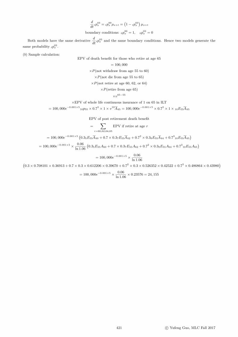
d
dttp
03x = tp
00x µx+t =
(1− tp
03x
)µx+t
boundary conditions: 0p00x = 1, 0p
03x = 0
Both models have the same derivative d
dttp
03x and the same boundary conditions. Hence two models generate the
same probability tp03x .
(b) Sample calculation:EPV of death benefit for those who retire at age 65
= 100, 000×P (not withdraw from age 55 to 60)×P (not die from age 55 to 65)×P (not retire at age 60, 62, or 64)
×P (retire from age 65)
×v65−55
×EPV of whole life continuous insurance of 1 on 65 in ILT= 100, 000e−0.001×5
10p55 × 0.73 × 1× v10A65 = 100, 000e−0.001×5 × 0.73 × 1× 10E55A65
EPV of post retirement death benefit
=∑
r=60,62,64,65
EPV if retire at age r
= 100, 000e−0.001×5 (0.35E55A60 + 0.7× 0.37E55A62 + 0.72 × 0.39E55A64 + 0.7310E55A65
)= 100, 000e−0.001×5 × 0.06
ln 1.06(0.35E55A60 + 0.7× 0.37E55A62 + 0.72 × 0.39E55A64 + 0.73
10E55A65)
= 100, 000e−0.001×5 × 0.06ln 1.06(
0.3× 0.708101× 0.36913 + 0.7× 0.3× 0.612206× 0.39670 + 0.72 × 0.3× 0.526352× 0.42522 + 0.73 × 0.486864× 0.43980)
= 100, 000e−0.001×5 × 0.06ln 1.06 × 0.23576 = 24, 155
421 c© Yufeng Guo, MLC Fall 2017


Chapter 52
Multiple state model: various problems
Example 52.0.1
In the basic survival model, 2px = 0.9. In the alive-dead model, calculate 2p
00x , 2p
01x , 2p
10x , 2p
11x , 2p
00x , 2p
11x .
alive 0 dead 1
Solution 52.0.1
2p00x = 2p
00x = 2px = 0.9 (once you leave state 1 and
can never go back in the alive-death model).2p
11x = 2p
11x = 1 (once dead, always dead).
2p01x = 2qx = 0.1, 2p
10x = 0 (can’t change from being
dead to alive),
force of transition or transition intensity
If the state variable Y (t) is continuous, then µijx = limh→0
hpijx
hfor i 6= j is called the force of transition or the transition
intensity between state i and state j for age x. This is the counterpart of the force of mortality in the basic alive-deadmodel and µ01
x = µx.
Example 52.0.2
In the alive(0)-dead(1) model, µ01x = lim
h→0
hp01x
h=
limh→0
hqxh
. Explain why µ01x is the force of mortality
µx.
Solution 52.0.2
See section 9.2.
Another way to express µijx = limh→0
hpijx
his hp
ijx = hµijx + o(h), where o(h) is a function that approaches zero faster
than h approaches zero. And for a small h, hpijx ≈ hµijx .
52.1 find probability of being stuck in a state
Example 52.1.1
A 10-year sickness policy is issued to a healthy life age50. The policy pays a no-claim bonus of 1000 at theend of Year 10 if the insured remains healthy through-out the term of the contract. The transition intensitiesare constants for all ages. δ = 0.06. Calculate the EPVof the bonus.
Healthy Sick
Dead
0 1
2
µ10x = 0.01
µ01x = 0.02
µ 02x=
0.04 µ12x
=0.0
8
Solution 52.1.1
The probability of receiving the bonus is 10p0050.
10p0050 = exp
(−∫ 10
0(µ01
50+s + µ0250+s)ds
)
= exp
(−∫ 10
0(0.02 + 0.04)ds
)= e−0.06(10) = e−0.6
EPV: 100010p0050e−10δ = 1000e−0.12 = 886.92
Example 52.1.2
The transition intensities are constants for all ages.Calculate the probability that (x) remains sickthroughout the next 3 years given that he’s sick today.
Healthy Sick
Dead
0 1
2
µ10x = 0.01
µ01x = 0.02
µ 02x=
0.04 µ12x
=0.0
8
423

Solution 52.1.2
3p11x = exp
(−∫ 3
0(µ10x+s + µ12
x+s)ds
) = e−3(0.09) = 0.7634
52.2 when getting back to a state is the same as being stuck in the state
tpiix = tp
iix holds under two situations: (1) you cannot leave a state (such as the death state), and (2) you can leave a
state, but if you leave then you can never get back. For any other situation, tpiix > tpiix .
Example 52.2.1
For which states does the equation tpiix = tp
iix hold?
Healthy Sick
Dead
0 1
2
µ01x
µ 02x µ12x
Solution 52.2.1
Clearly, tp22x = tp
22x ; once dead, always dead.
If you leave state 0, you can’t get back. tp00x = tp
00x .
Example 52.2.2
For which states does the equation tpiix = tp
iix hold?
Healthy Sick
Dead
0 1
2
µ10x
µ01x
µ 02x µ12x
Solution 52.2.2
Only the “dead” state satisfies the equation and tp22x =
tp22x . For the other states, tp00
x > tp00x and tp
11x > tp
11x .
Example 52.2.3
For which states does the equation tpiix = tp
iix hold?
Alive Dead0 1
µ01x
Solution 52.2.3
Both the “alive” and the “dead” states satisfy the equa-tion tp
iix = tp
iix .
52.3 getting back and being stuck, various transition probabilities
In a word problem, it may not be immediately clear whether you should use tpiix or tpiix . If re-entry to state i is impossible,then tp
iix = tp
iix and it doesn’t matter which one you use. However, if re-entry is possible, then tp
iix 6= tp
iix and water gets
muddy. Ask “Is re-entry to state i allowed in the event?” If YES, use tpiix . If NO, then use tp
iix .
Example 52.3.1
A 10-year sickness policy on a healthy life (50) pays100,000 at the moment when the insured becomes sick.δ = 0.06. Calculate the EPV of this policy.
Healthy Sick
Dead
0 1
2
µ01x = 0.02
µ 02x=
0.04 µ12x
=0.0
8
Solution 52.3.1
The death benefit is paid at t if the insured
• is still in state 0 at t, prob: tp0050
• transitions to state 1 during [t, t + dt], prob:µ01
50+tdt
100000∫ 10
0e−δttp
0050µ
0150+tdt = 100000
∫ 10
0e−δttp
0050µ
0150+tdt
= 100000∫ 10
0e−0.06te−(0.02+0.04)t0.02dt
= 100000× 212
(1− e−0.12×10) = 11646.763

Example 52.3.2
The transition intensities are constants for all ages.Calculate the probability that a healthy life (x) todayis still healthy 10 years from today.
Healthy Disabled
Dead
0 1
2
µ01x = 0.06
µ 02x=
0.02 µ12x
=0.0
4
Solution 52.3.2
10p00x = 10p
00x = e−(0.06+0.02)10 = e−0.8.
Example 52.3.3
The transition intensities are constants for all ages. Calculate the probability that a healthy life (x) today is disabled10 years from today.
Healthy Disabled
Dead
0 1
2
µ01x = 0.06
µ 02x=
0.02 µ12x
=0.0
4
Solution 52.3.3
We want to start from state 0 today and be at state 1 at t = 10. We can
• hang out at state 0 during [0, t], prob: tp00x = e−0.08t
• go to state 1 during [t, t+ dt], prob: dtp01x+t = µ01
x+tdt+ o(dt) ≈ 0.06dt
• hang out in state 1 during [t+ dt, 10] ≈ [t, 10], prob: 10−tp11x+t = e−0.04(10−t)
10p01x =
∫ 10
0tp
00x µ
01x+t10−tp
11x+tdt
=∫ 10
0e−0.08t0.06e−0.04(10−t)dt = 0.06e−0.4
∫ 10
0e−0.04tdt = 6e−0.4
4(1− e−0.4) = 0.3315
Example 52.3.4
The transition intensities are constants for all ages. A healthy insured is age x today. Let A represent the probabilitythat the insured is dead 10 years from today and he’s disabled at death. Calculate A.
Healthy Disabled
Dead
0 1
2
µ01x = 0.06
µ 02x=
0.02 µ12x
=0.0
4
Solution 52.3.4
We want to complete the path 0→ 1→ 2 in 10 years or less.
A =∫ 10
0tp
01x µ
12x+t10−tp
22x+tdt =
∫ 10
0tp
01x µ
12x+tdt
From the previous problem,
mp01x =
∫ m
0tp
00x µ
01x+tm−tp
11x+tdt
=∫ m
0e−0.08t0.06e−0.04(m−t)dt = 0.06e−0.04m
∫ m
0e−0.04tdt = 0.06
0.04(e−0.04m − e−0.08m)
A =∫ 10
0tp
01x µ
12x+tdt =
∫ 10
0
0.060.04
(e−0.04t − e−0.08t) 0.08dt = 0.12
(1− e−0.4
0.04 − 1− e−0.8
0.08
)= 0.16303
425 c© Yufeng Guo, MLC Fall 2017

Example 52.3.5
The transition intensities are constants for all ages. Ahealthy insured is age x today. Let B represent theprobability that the insured is dead 10 years from to-day and he’s healthy at death. Calculate B.
Healthy Disabled
Dead
0 1
2
µ01x = 0.06
µ 02x=
0.02 µ12x
=0.0
4
Solution 52.3.5
We want to complete the path 0 → 2 in 10 years orless.
B =∫ 10
0tp
00x µ
02x+tdt =
∫ 10
0tp
00x µ
02x+tdt
=∫ 10
0e−0.08t0.02dt = 0.021− e−0.8
0.08 = 0.1377
Example 52.3.6
The transition intensities are constants for all ages. Ahealthy insured is age x today. Let C represent theprobability that the insured is dead 10 years from to-day.
Healthy Disabled
Dead
0 1
2
µ01x = 0.06
µ 02x=
0.02 µ12x
=0.0
4
Solution 52.3.6
C = A+B = 0.16303 + 0.1377 = 0.30073
Example 52.3.7
The transition intensities are constants for all ages.Calculate the probability that a healthy life (x) todayis still healthy 10 years from today. Is it 10p
00x or 10p
00x ?
Healthy Disabled
Dead
0 1
2
µ10x = 0.01
µ01x = 0.06
µ 02x=
0.02 µ12x
=0.0
4
Solution 52.3.7
Now 10p00x > 10p
00x . Which one to use?
When you count the number of people still healthyat t = 10, should you include those who return to thehealthy state after recovering from prior disabilities?Yes you should. Then the probability is 10p
00x .
There’s no closed-form formula for 10p00x . We can
use the Euler method to approximate 10p00x .
Example 52.3.8
The transition intensities are constants for all ages.Calculate the probability that a healthy life (x) todayis ever disabled during the next 10 years.
Healthy Disabled
Dead
0 1
2
µ10x = 0.01
µ01x = 0.06
µ 02x=
0.02 µ12x
=0.0
4
Solution 52.3.8
The insured can travel back and forth between state0 and state 1 repeatedly and have many disability re-lapses. Do disability relapses matter in this problem?Surprisingly NO. The event “ever being disabled” is thesame as walking through the path 0→ 1 at least once,which is the same as having the 1st period of disability.We can simplify the diagram into:
Healthy Disabled
Dead
0 1
2
µ01x = 0.06
µ 02x=
0.02 µ12x
=0.0
4
The insured can (1) hang out at state 0 during [0, t],prob: tp
00x , and (2) move from state 0 to 1 in the next
instant, prob: µ01x+tdt. The probability of making these
two moves is p(t) = tp00x µ
01x+tdt. Next, sum p(t) from
t = 0 to t = 10:∫ 10
0 tp00x µ
01x+tdt =
∫ 100 e−0.08t0.06dt =
68(1− e−0.8) = 0.4130.
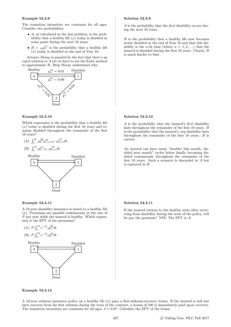
Example 52.3.9
The transition intensities are constants for all ages.Consider two probabilities:• A, as calculated in the last problem, is the prob-
ability that a healthy life (x) today is disabled atsome point during the next 10 years.• B = 10p
01x is the probability that a healthy life
(x) today is disabled at the end of Year 10.Actuary Moray is puzzled by the fact that there’s an
exact solution to A yet we have to use the Euler methodto approximate B. Help Moray understand why.
Healthy Disabled
Dead
0 1
2
µ10x = 0.01
µ01x = 0.06
µ 02x=
0.02 µ12x
=0.0
4
Solution 52.3.9
A is the probability that the first disability occurs dur-ing the next 10 years.
B is the probability that a healthy life now becomesnewly disabled at the end of Year 10 and that this dis-ability is the n-th time (where n = 1, 2, . . .) that theinsured is disabled during the first 10 years. Clearly, Bis much harder to find.
Example 52.3.10
Which expression is the probability that a healthy life(x) today is disabled during the first 10 years and re-mains disabled throughout the remainder of the first10 years?
(A)∫ 10
0 tp00x µ
01x+t10−tp
11x+tdt
(B)∫ 10
0 tp01x 10−tp
11x+tdt
Healthy Disabled
Dead
0 1
2
Solution 52.3.10
A is the probability that the insured’s first disabilitylasts throughout the remainder of the first 10 years. Bis the probability that the insured’s any disability laststhroughout the remainder of the first 10 years. B iscorrect.
An insured can have many “healthy this month, dis-abled next month” cycles before finally becoming dis-abled continuously throughout the remainder of thefirst 10 years. Such a scenario is discarded in A butis captured in B.
Example 52.3.11
A 10-year disability insurance is issued to a healthy life(x). Premiums are payable continuously at the rate ofP per year while the insured is healthy. Which expres-sion is the EPV of the premiums?
(A) P∫ 10
0 e−δttp00x dt
(B) P∫ 10
0 e−δttp00x dt
Healthy Disabled
Dead
0 1
2
Solution 52.3.11
If the insured returns to the healthy state after recov-ering from disability during the term of the policy, willhe pay the premium? YES. The EPV is A.
Example 52.3.12
A 10-year sickness insurance policy on a healthy life (x) pays a first-sickness-recovery bonus. If the insured is sick butlater recovers from his first sickness during the term of the contract, a bonus of 100 is immediately paid upon recovery.The transition intensities are constants for all ages. δ = 0.07. Calculate the EPV of the bonus.
427 c© Yufeng Guo, MLC Fall 2017

Healthy Sick
Dead
0 1
2
µ10x = 0.01
µ01x = 0.06
µ 02x=
0.02 µ12x
=0.0
4
Solution 52.3.12
The bonus is paid if the insured walks through the path 0→ 1→ 0 in 10 years. The insured needs to do the following:
• stay in state 0 during [0, t], prob: tp00x ,
• transition to state 1 during [t, t+ dt], prob: µ01x+tdt,
• stay in state 1 during [t, t+ u], prob: up11x+t, and finally
• transition to state 0 during [t+ u, t+ u+ du], prob: µ10x+t+udu
After making the above moves, the insured will get the bonus is at t+ u. The constraints are
t ≥ 0, u ≥ 0, 0 ≤ t+ u ≤ 10
100∫ 10
t=0
∫ 10−t
u=0e−δ(t+u)
tp00x µ
01x+tup
11x+tµ
10x+t+ududt
= 100∫ 10
t=0
∫ 10−t
u=0e−0.07(t+u)e−0.08t0.06e−0.05u0.01dudt
= 0.06∫ 10
0e−0.15t
∫ 10−t
0e−0.12ududt = 0.06
∫ 10
0
1− e−0.12(10−t)
0.12 e−0.15tdt
= 0.5
(∫ 10
0e−0.15tdt− e−1.2
∫ 10
0e−0.03tdt
)
= 0.5(
1− e−1.5
0.15 − e−1.2 1− e−0.3
0.03
)= 1.2885
52.4 Check your knowledge
Homework 52.4.1
(MLC: Spring 2016 Q4) A 5-year sickness insurance policy is based on the following Markov model:
Healthy Sick
Dead
0 1
2
You are given the following constant forces of transition:
(i) µ01 = 0.05
(ii) µ10 = 0.02
(iii) µ02 = 0.01
(iv) µ12 = 0.06
Calculate the probability that a Healthy life will become Sick exactly once during the 5 years and remain continuouslySick from that point until the end of the 5 years.
Homework Solution 52.4.1

Difficulty
∫ 5
0tp
00x µ
01x+t5−tp
11x+tdt =
∫ 5
0e−(0.05+0.01)t0.05e−(5−t)(0.02+0.06)dt = 0.17624544
Homework 52.4.2
(spring 2012 MLC Q12) Employees in Company ABC can be in:
State 0: Non-executive employee
State 1: Executive employee
State 2: Terminated from employment
John joins Company ABC as a non-executive employee at age 30. You are given:
(i) µ01 = 0.01 for all years of service
(ii) µ02 = 0.06 for all years of service
(iii) µ12 = 0.02 for all years of service
(iv) Executive employees never return to the non-executive employee state.
(v) Employees terminated from employment never get rehired.
(vi) The probability that John lives to age 65 is 0.9, regardless of state.
Calculate the probability that John will be an executive employee of Company ABC at age 65.
Homework Solution 52.4.2
Difficulty
Non Exe
Fired
0 1
2
0.01
0.06 0.02
The probability that John will be an executive employee of Company ABC at age 65 is:
35p30 × 35p0130 = 0.935p
013035p
0130 =
∫ 35
0tp
0030µ
0130+t35−tp
1130+tdt =
∫ 35
0e−(0.01+0.06)t0.01e−0.02(35−t)dt = 0.258
0.9(0.258) = 0.2322
Homework 52.4.3
(MLC: Spring 2014 Q3) A continuous Markov process is modeled by the following multiple state diagram:
state 0 state 1
state 2
You are given the following constant transition intensities:
(i) µ01 = 0.08
(ii) µ02 = 0.04
(iii) µ10 = 0.10
(iv) µ12 = 0.05
For a person in State 1, calculate the probability that the person will continuously remain in State 1 for the next 15years.
Homework Solution 52.4.3
429 c© Yufeng Guo, MLC Fall 2017

Difficulty
15p11x = exp
(−∫ 15
0(µ10x+s + µ12
x+s)ds
)= e−15(0.15) = 0.1054
Homework 52.4.4
(Exam MLC: Spring 2012 Q28) You are using Euler’s method to calculate estimates of probabilities for a multiple statemodel with states 0, 1, 2. You are given:
(i) The only possible transitions between states are: 0 to 1, 1 to 0, and 1 to 2
(ii) For all x, µ01x = 0.3, µ10
x = 0.1, µ12x = 0.1
(iii) Your step size is 0.1.
(iv) You have calculated that 0.6p00x = 0.8370, 0.6p
01x = 0.1588, 0.6p
02x = 0.0042,
Calculate the estimate of 0.8p01x using the specified procedure.
0 1
2
µ10x = 0.1
µ01x = 0.3
µ12x
=0.1
Homework Solution 52.4.4
Difficulty
d
dttp
00x = t
[tp
01x µ
10x+t − tp
00x µ
01x+t
]= t[0.1tp01
x − 0.3tp00x
]d
dttp
01x = t
[tp
00x µ
01x+t − tp
01x (µ10
x+t + µ12x+t)
]= t[0.3tp00
x − 0.2tp01x
]0.7p
00x ≈ 0.6p
00x + 0.1(0.10.6p
01x − 0.30.6p
00x ) = 0.8370 + 0.1(0.1(0.1588)− 0.3(0.8370)) = 0.813478
0.7p01x ≈ 0.6p
01x + 0.1(0.30.6p
00x − 0.20.6p
01x ) = 0.1588 + 0.1(0.3(0.8370)− 0.2(0.1588)) = 0.180734
0.8p01x ≈ 0.7p
01x + 0.1(0.30.7p
00x − 0.20.7p
01x ) = 0.180734 + 0.1(0.3(0.813478)− 0.2(0.180734)) = 0.20152366
Homework 52.4.5
A disability insurance is issued to healthy life (x). The transition intensities are constants for all ages. Let the contractissue time be time zero. Use the Euler method. Set h = 1/12.
• 3hp00x , 3hp
01x , 3hp
11x , 3hp
10x
• estimate 3hp00x − 3hp
00x
Healthy Disabled
Dead
0 1
2
µ10x = 0.01
µ01x = 0.02
µ 02x=
0.03 µ12x
=0.0
6
Homework Solution 52.4.5
Difficulty
t tp00x tp
01x tp
02x
0 1.00000 0.00000 0.00000h 0.99583 0.00167 0.002502h 0.99169 0.00332 0.005003h 0.98756 0.00495 0.00749

3hp00x =
∫ 3/12
0e−0.05tdt = 1− e−0.05×3/12
0.05 = 0.24844
3hp00x − 3hp
00x = 0.98756− 0.24844 = 0.73912
Homework 52.4.6
A 10-year disability insurance policy is issued to healthy life (x). The policy pays 100,000 immediately at the onset ofdisability.
Healthy Disability
Dead
0 1
2
µ10x
µ01x
µ 02x µ12x
Which expression is the EPV for this policy?
(A) 100000∫ 10
0 e−δttp00x µ
01x+tdt
(B) 100000∫ 10
0 e−δttp00x µ
01x+tdt
Homework Solution 52.4.6
DifficultyA is correct. The insured can be newly disabled many times during the term of the contract and each new disabilitytriggers the benefit. A counts for this while B is the EPV of the benefit for the first disability during the term of thecontract. There’s no exact way to calculate the integral 100000
∫ 100 e−δttp
00x µ
01x+tdt as there’s no exact way to find tp
00x .
Homework 52.4.7
A combined 10-year term life and disability insurance policy is issued to healthy life (x). The policy pays 100,000immediately on death or the onset of disability. No further benefit is paid in the event of death after a prior disabilityclaim has been paid.
The transition intensities are constants for all ages. δ = 0.05. Calculate the EPV of this policy.
Healthy Disability
Dead
0 1
2
µ01x = 0.004
µ 02x=
0.002 µ12x
=0.0
08
Homework Solution 52.4.7
DifficultyWe can ignore path 1→ 2 because death after disability will not trigger the death benefit.
100000∫ 10
0e−δttp
00x (µ01
x+t + µ02x+t)dt = 100000
∫ 10
0e−δttp
00x (µ01
x+t + µ02x+t)dt
= 100000∫ 10
0e−0.05te−0.006t0.006dt = 100000
∫ 10
0e−0.056t0.006dt = 100000× 6
56(1− e−0.056×10) = 4594.1886
Homework 52.4.8
Same as the last problem EXCEPT that the limitation “no further benefit is paid in the event of death after a priordisability claim has been paid” is removed. Calculate the EPV of this policy.
Homework Solution 52.4.8
431 c© Yufeng Guo, MLC Fall 2017

DifficultyMETHOD 1. EPV of the death benefit if the insured is healthy at death:
100000∫ 10
0e−δttp
00x µ
02x+tdt = 100000
∫ 10
0e−0.05te−0.006t0.002dt = 100000× 2
56(1− e−0.56) = 1531.3962
EPV of the disability benefit if the insured is continuously disabled throughout the remainder of the 10-year term:
100000∫ 10
0e−δttp
00x µ
01x+t10−tp
11x+tdt = 100000
∫ 10
0e−0.05te−0.006t0.004e−(10−t)0.008dt
= 100000(0.004)e−0.08∫ 10
0e−0.048tdt = 100000(0.004)e−0.08 1− e−0.48
0.048 = 2932.5607
The insured will get paid twice if he walks through the path 0 → 1 → 2 during the 10-year term: (1) the disabilitybenefit 100,000 at t, and (2) the death benefit 100,000 at t+ u if he makes the following moves:
(a) is continuously healthy during [0, t]; prob: tp00x = e−0.006t
(b) becomes disabled during [t, t+ dt]; prob: µ01x+tdt = 0.004dt
(c) is continuously disabled during [t+ dt, t+ dt+ u] ≈ [t, t+ u]; prob: up11x+t = e−0.008u
(d) moves to state 2 during [t+ u, t+ u+ du], prob: µ12x+t+udu = 0.008du.
For each (t, u) pair where 0 < t+ u < 10, the EPV of the double payments is
g(t, u) = 100, 000(e−δt + e−δ(t+u))e−0.006t0.004e−0.008u0.008dudt
∫ 10
t=0
∫ 10−t
u=0g(t, u) = 100, 000
∫ 10
t=0
∫ 10−t
u=0(e−0.05t + e−0.05(t+u))e−0.006t0.004e−0.008u0.008dudt
= 100000(0.004)(0.008)∫ 10
0e−0.056t
(∫ 10−t
0(1 + e−0.05u)e−0.008udu
)dt = 240.6666
Total EPV : 1531.3962 + 2932.5607 + 240.6666 = 4704.6235
If double payments are not allowed, the EPV for death after disability is
100, 000∫ 10
t=0
∫ 10−t
u=0(e−0.05t + 0)e−0.006t0.004e−0.008u0.008dudt = 130.23171
Total EPV : 1531.3962 + 2932.5607 + 130.23171 = 4594.1886
METHOD 2. EPV of the death benefit if the insured is disabled at death:
100000∫ 10
0
∫ 10−t
0e−δ(t+u)
tp00x µ
01x+tup
11x+tµ
12x+t+ududt = 100000
∫ 10
0
∫ 10−t
0e−0.05(t+u)e−0.006t0.004e−0.008u0.008dudt = 110.4349
Total EPV : 4594.1886 + 110.4349 = 4704.6235
Homework 52.4.9
A pension plan provides a benefit of 100,000 payable on death regardless of whether death occurs before or afterretirement. The transition intensities are constants for all ages. δ = 0.05. Calculate the EPV of this policy for an activemember currently age x.
Active Retired
Dead
0 1
2
µ01x = 0.9
µ 02x=
0.02 µ12x
=0.0
6
Homework Solution 52.4.9

DifficultyEPV for the path 0→ 2:
100000∫ ∞
0e−δttp
00x µ
02x+tdt = 100000
∫ ∞0
e−0.05te−0.92t0.02dt = 2061.8557
EPV for the path 0→ 1→ 2 (the death benefit is paid at age x+ t+ u):
100000∫ ∞
0tp
00x µ
01x+t
∫ ∞0
e−δ(t+u)up
11x+tµ
12x+t+ududt
= 100000∫ ∞
0e−0.92t0.9
∫ ∞0
e−0.05(t+u)e−0.06u0.06dudt
= 100000× 0.9× 0.06∫ ∞
0e−0.97tdt
∫ ∞0
e−0.11udu
= 100000× 0.9× 0.060.97× 0.11 = 50609.185
Total: 2061.8557 + 50609.185 = 52671.041
Homework 52.4.10
(Exam MLC: Fall 2013 Q10) Calculate the conditional probability that a Healthy life on January 1, 2004 is still Healthyon January 1, 2014, given that this person is not Dead on January 1, 2014.
Healthy Disabled
Dead
0 1
2
µ01 = 0.02µ 02
=0.03 µ
12=
0.05
Homework Solution 52.4.10
DifficultyA =healthy today and healthy 10 years from today. B =healthy today, disabled at some point during the next 10 yearsand remain disabled during the reminder of the 10 year period.
P (A) = 10p00x = 10p
00x = e−(µ01+µ02)10 = e−0.05×10 = e−0.5
P (B) =∫ 10
0tp
00x µ
0110−tp
11x+tdt
=∫ 10
0e−(µ01+µ02)tµ01e−µ
12(10−t)dt =∫ 10
0e−0.05t0.02e−0.05(10−t)dt = 0.2e−0.5
P (A | A⋃
B) = P (A)P (A) + P (B) = 1
1 + 0.2 = 0.8333
Homework 52.4.11
(Exam MLC: Fall 2013 Q21) You are pricing an automobile insurance on (x). The insurance pays 10,000 immediatelyif (x) gets into an accident within 5 years of issue. The policy pays only for the first accident and has no other benefits.
(i) You model (x)’s driving status as a multi-state model with the following 3 states:
0 1
2
0 - low risk, without an accident1 - high risk, without an accident2 - has had an accident
(ii) (x) is initially in state 0.
433 c© Yufeng Guo, MLC Fall 2017

(iii) The following transition intensities for 0 ≤ t ≤ 5
µ01x+t = 0.20 + 0.10t
µ02x+t = 0.05 + 0.05t
µ12x+t = 0.15 + 0.01t2
(iv) 3p01x = 0.4174
(v) δ = 0.02
(vi) The continuous function g(t) is such that the expected present value of the benefit up to time a equals∫ a
0 g(t)dt,0 ≤ a ≤ 5, where t is the time of the first accident.
Calculate g(3).
Homework Solution 52.4.11
Difficulty
The most difficult task is to figure out what g(t) means. g(t) is the EPV of the single claim at t. A claim occurswhen state 0 or 1 moves to state 2.
g(t) = 10000e−δt(tp00x µ
02x+t + tp
01x µ
12x+t)
g(3) = 10000e−3δ(3p00x µ
02x+3 + 3p
01x µ
12x+3)
You are already given 3p01x = 0.4174
3p00x = 3p
00x = exp
(−∫ 3
0(µ01x+t + µ02
x+t)dt
)
= exp
(−∫ 3
0(0.20 + 0.10t+ 0.05 + 0.05t)dt
)= e−1.425
3p00x µ
02x+3 + 3p
01x µ
12x+3 = e−1.425(0.05 + 0.05× 3) + 0.4174(0.15 + 0.01× 32) = 0.148276
g(3) = 10000e−0.02×30.148276 = 1396.4108
Homework 52.4.12
(Exam MLC: Fall 2012 Q12) A party of scientists arrives at a remote island. Unknown to them, a hungry tyrannosaurlives on the island. You model the future lifetimes of the scientists as a three-state model, where:
0 - State 0: no scientists have been eaten.
1 - State 1: exactly one scientist has been eaten.
2 - State 2: at least two scientists have been eaten.
0 1
2
You are given:
(i) Until a scientist is eaten, they suspect nothing, so µ01t = 0.01 + 0.02× 2t, t > 0
(ii) Until a scientist is eaten, they suspect nothing, so the tyrannosaur may come across two together and eat both,with µ02
t = 0.5µ01t , t > 0
(iii) After the first death, scientists become much more careful, so µ12t = 0.01, t > 0
Calculate the probability that no scientists are eaten in the first year.
Homework Solution 52.4.12

Difficulty
1p00x = 1p
00x = exp
(−∫ 1
0(µ01x+t + µ02
x+t)dt
)= exp
(−∫ 1
01.5µ01
x+tdt
)∫ 1
01.5µ01
x+tdt =∫ 1
01.5(0.01 + 0.02× 2t)dt
= 1.5(
0.01t+ 0.02× 2t
ln 2
)1
0= 1.5
(0.01 + 0.02
ln 2
)= 0.05828
1p00x = e−0.05828 = 0.9434
Homework 52.4.13
(Exam MLC: Fall 2012 Q16) You are evaluating the financial strength of companies based on the following multiplestate model:
Solvent Bankrupt
Liquidated
0 1
2
For each company, you assume the following constant transition intensities:
(i) µ01 = 0.02
(ii) µ10 = 0.06
(iii) µ12 = 0.10
Using Kolmogorov’s forward equation with step h = 1/2, calculate the probability that a company currently Bankruptwill be Solvent at the end of one year.
Homework Solution 52.4.13
Difficulty
d
dttp
10x = tp
11x µ
10x+t − tp
10x µ
01x+t = 0.06tp11
x − 0.02tp10x
,
d
dttp
10x
∣∣∣t=0
= 0.06(1)− 0.02(0) = 0.06
,
d
dttp
11x = tp
10x µ
01x+t − tp
11x (µ10
x+t + µ12x+t) = 0.02tp10
x − 0.16tp11x
,
d
dttp
11x
∣∣∣t=0
= 0.2(0)− 0.16(1) = −0.16
,
hp10x ≈ 0p
10x + h
d
dttp
10x
∣∣∣t=0
= 0 + 0.06/2 = 0.03
hp11x ≈ 0p
11x + h
d
dttp
11x
∣∣∣t=0
= 1− 0.16/2 = 0.92
d
dttp
10x
∣∣∣t=h
= 0.06(0.92)− 0.02(0.03) = 0.0546
,
2hp10x ≈ hp
10x + h
d
dttp
10x
∣∣∣t=h
= 0.03 + 0.0546/2 = 0.0573
Homework 52.4.14
435 c© Yufeng Guo, MLC Fall 2017
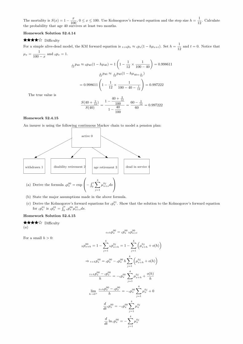
The mortality is S(x) = 1− x
100 , 0 ≤ x ≤ 100. Use Kolmogorov’s forward equation and the step size h = 112 . Calculate
the probability that age 40 survives at least two months.
Homework Solution 52.4.14
DifficultyFor a simple alive-dead model, the KM forward equation is t+hpx ≈ tpx(1− hµx+t). Set h = 1
12 and t = 0. Notice that
µx = 1100− x and 0px = 1.
112p40 ≈ 0p40(1− hµ40) = 1
(1− 1
12 ×1
100− 40
)= 0.998611
212p40 ≈ 1
12p40(1− hµ40+ 1
12)
= 0.998611
(1− 1
12 ×1
100− 40− 112
)= 0.997222
The true value is
S(40 + 212 )
S(40) =1−
40 + 212
1001− 40
100
=60− 2
1260 = 0.997222
Homework 52.4.15
An insurer is using the following continuous Markov chain to model a pension plan:
active 0
withdrawn 1 disability retirement 2 age retirement 3 dead in service 4
(a) Derive the formula tp00x = exp
− ∫ t0 4∑j=1
µ0jx+sds
(b) State the major assumptions made in the above formula.
(c) Derive the Kolmogorov’s forward equations for tp01x . Show that the solution to the Kolmogorov’s forward equation
for tp01x is tp01
x =∫ t
0 sp00x µ
01x+sds.
Homework Solution 52.4.15
Difficulty(a)
t+hp00x = tp
00x hp
00x+t
For a small h > 0:
hp00x+h = 1−
4∑j=1
hp0jx+h = 1−
4∑j=1
(µ0jx+h + o(h)
)
⇒ t+hp00x = tp
00x − tp
00x h
4∑j=1
(µ0jx+h + o(h)
)t+hp
00x − tp
00x
h= −tp00
x
4∑j=1
µ0jx+h + o(h)
h
limh→0+
t+hp00x − tp
00x
h= −tp00
x
4∑j=1
µ0jx + 0
d
dttp
00x = −tp00
x
4∑j=1
µ0jx
d
dtln tp00
x = −4∑j=1
µ0jx

Integrate both sides and use the boundary condition 0p00x = 1:
tp00x = exp
−∫ t
0
4∑j=1
µ0jx+sds
(b) Major assumptions:
• transition probabilities depend only on the current age and the current state (Markov property)
• P (transitions in a short intervals h = 0)
(c)t+hp
01x = tp
01x hp
11x+t + tp
00x hp
01x+t = tp
01x + tp
00x hp
01x+t because hp
11x+t = 1
µ01x = lim
h→0+
hp01x
hdefinition → hp
01x = hµ01
x + o(h), hp01x+t = hµ01
x+t + o(h)
t+hp01x − tp
01x = h tp
00x µ
01x+t + o(h)
d
dttp
01x = lim
h→0+
t+hp01x − tp
01x
h= tp
00x µ
01x+t
The above formula is the Kolmogorov’s forward equations for tp01x . Integrate both sides of the above formula from t = 0
to t:
tp01x − 0p
01x =
∫ t
0sp
00x µx+sds
0p01x = 0, ⇒ tp
01x =
∫ t
0sp
00x µx+sds
Homework 52.4.16
(4 points) For the following Markov model, derive the following Kolmogorov’s forward equations:
(a) d
dttp
02x = tp
00x µ
02x+t + tp
01x µ
12x+t
(b) d
dttp
01x = tp
00x µ
01x+t − tp
01x
(µ10x+t + µ12
x+t)
Healthy Sick
Dead
0 1
2
µ10x
µ01x
µ 02x µ12x
Homework Solution 52.4.16
Difficulty(a)
t+hp02x = tp
00x hp
02x+t + tp
01x hp
12x+t + tp
02x hp
22x+t
hp22x+t = 0. For a small h > 0:
hp02x+t = hµ02
x+t + o(h), hp12x+t = hµ12
x+t + o(t)
t+hp02x = tp
00x hµ02
x+t + tp01x hµ12
x+t + tp02x + o(h)
t+hp02x − tp
02x
ht+hp
02x = tp
00x µ02
x+t + tp01x µ12
x+t + o(h)h
limh→0+
t+hp02x − tp
02x
h= tp
00x µ02
x+t + tp01x µ12
x+t + 0
⇒ d
dttp
02x = tp
00x µ
02x+t + tp
01x µ
12x+t
(b)t+hp
01x = tp
00x hp
01x+t + tp
01x hp
11x+t
hp01x+t = hµ01
x+t + o(h)
hp11x+t = 1−
(hp
10x+t + hp
12x+t)
= 1− h(µ10x+t + µ12
x+t)
+ o(h)
437 c© Yufeng Guo, MLC Fall 2017
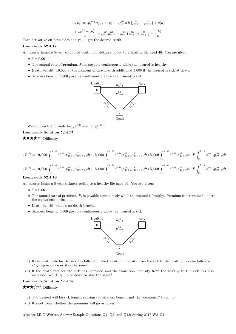
t+hp01x = tp
00x hµ01
x+t + tp01x − tp
01x hh
(µ10x+t + µ12
x+t)
+ o(h)
t+hp01x − tp
01x
h= tp
00x µ01
x+t − tp01x
(µ10x+t + µ12
x+t)
+ o(h)h
Take derivative on both sides and you’ll get the desired result.
Homework 52.4.17
An insurer issues a 5-year combined death and sickness policy to a healthy life aged 40. You are given:
• δ = 0.06• The annual rate of premium, P , is payable continuously while the insured is healthy• Death benefit: 10,000 at the moment of death, with additional 5,000 if the insured is sick at death• Sickness benefit: 5,000 payable continuously while the insured is sick
Healthy Sick
Dead
0 1
2
µ10x+t
µ01x+t
µ 02x+t µ
12x+t
Write down the formula for kV (0) and for kV (1).
Homework Solution 52.4.17
Difficulty
kV(0) = 10, 000
∫ 5−k
0e−δttp
0040+kµ
0240+k+tdt+15, 000
∫ 5−k
0e−δttp
0140+kµ
1240+k+tdt+5, 000
∫ 5−k
0e−δttp
0140+kdt−P
∫ 5−k
0e−δttp
0040+kdt
kV(1) = 10, 000
∫ 5−k
0e−δttp
1040+kµ
0240+k+tdt+15, 000
∫ 5−k
0e−δttp
1140+kµ
1240+k+tdt+5, 000
∫ 5−k
0e−δttp
1140+kdt−P
∫ 5−k
0e−δttp
1040+kdt
Homework 52.4.18
An insurer issues a 5-year sickness policy to a healthy life aged 40. You are given:
• δ = 0.06• The annual rate of premium, P , is payable continuously while the insured is healthy. Premium is determined under
the equivalence principle.• Death benefit: there’s no death benefit.• Sickness benefit: 5,000 payable continuously while the insured is sick
Healthy Sick
Dead
0 1
2
µ10x+t
µ01x+t
µ 02x+t µ
12x+t
(a) If the death rate for the sick has fallen and the transition intensity from the sick to the healthy has also fallen, willP go up or down or stay the same?
(b) If the death rate for the sick has increased and the transition intensity from the healthy to the sick has alsoincreased, will P go up or down or stay the same?
Homework Solution 52.4.18
Difficulty
(a) The insured will be sick longer, causing the sickness benefit and the premium P to go up.(b) It’s not clear whether the premium will go or down.
Also see MLC Written Answer Sample Questions Q4, Q5, and Q12; Spring 2017 WA Q1.

52.5 Today’s challenge
Homework 52.5.1
An insurance company uses the following continuousMarkov model for pricing a combined 20-year disabil-ity, annuity, and life insurance contract.
Healthy Disabled
Dead
0 1
2
µ10x = 0.02
µ01x = 0.04
µ 02x=
0.06 µ12x
=0.0
9
The policy is issued to a healthy life age (x).
The transition intensities are constants for all ages.
δ = 0.05
Calculate the EPV of each benefit separately.
Note. Not all benefits can be valued exactly. Ifthe exact numerical solution might not exit, just writedown the integral form for that EPV.
(A) 1000 per year payable continuously while the in-sured is healthy
(B) 1000 per year payable continuously while the in-sured is healthy but no payment is made if theinsured is healthy after recovering from disability
(C) 1000 payable at the moment of death
(D) 1000 payable immediately when the insured is dis-abled for the 1st time
(E) 1000 payable immediately upon death or disabil-ity but no death benefit is paid if there’s a priordisability claim
(F) 1000 per year payable continuously while the in-sured is disabled
(G) 1000 per year payable continuously throughoutthe 1st period of disability
(H) 1000 per year payable continuously throughoutthe 1st period of disability subject to a 6-monthwaiting period
(I) 1000 payable at the moment of death and an ad-ditional 500 if the insured was disabled at death
(J) a 1000 no-claim bonus payable at the end of theterm if there’s no death or disability claim duringthe term
(K) 1000 per year payable continuously while theinsured is continuously disabled in excess of 6months. However, any benefit period is limitedto 5 years, but the number of the benefit periodscan be unlimited.
439 c© Yufeng Guo, MLC Fall 2017


![From Objective to Subjective Di culty Evaluation in Video Games · 2018-11-22 · optimal level of challenge, and thus, to the game’s di culty [7]. Jesper Juul provided insight](https://img.pdfslide.net/doc/110x75/5ecad5b0600730616c18154b/from-objective-to-subjective-di-culty-evaluation-in-video-games-2018-11-22-optimal.jpg)