Embed Size (px)
Citation preview
Quiz 1 on Wednesday
• ~20 multiple choice or short answer questions
• In class, full period
• Only covers material from lecture, with a bias towards topics not covered by projects
• Study strategy: Review the slides and consult textbook to clarify confusing parts.

Project 3 preview
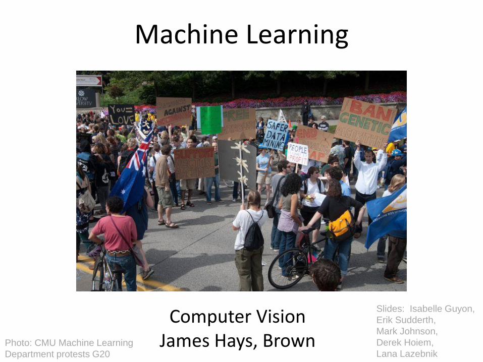
Machine Learning
Computer Vision
James Hays, Brown
Slides: Isabelle Guyon,
Erik Sudderth,
Mark Johnson,
Derek Hoiem,
Lana Lazebnik Photo: CMU Machine Learning
Department protests G20
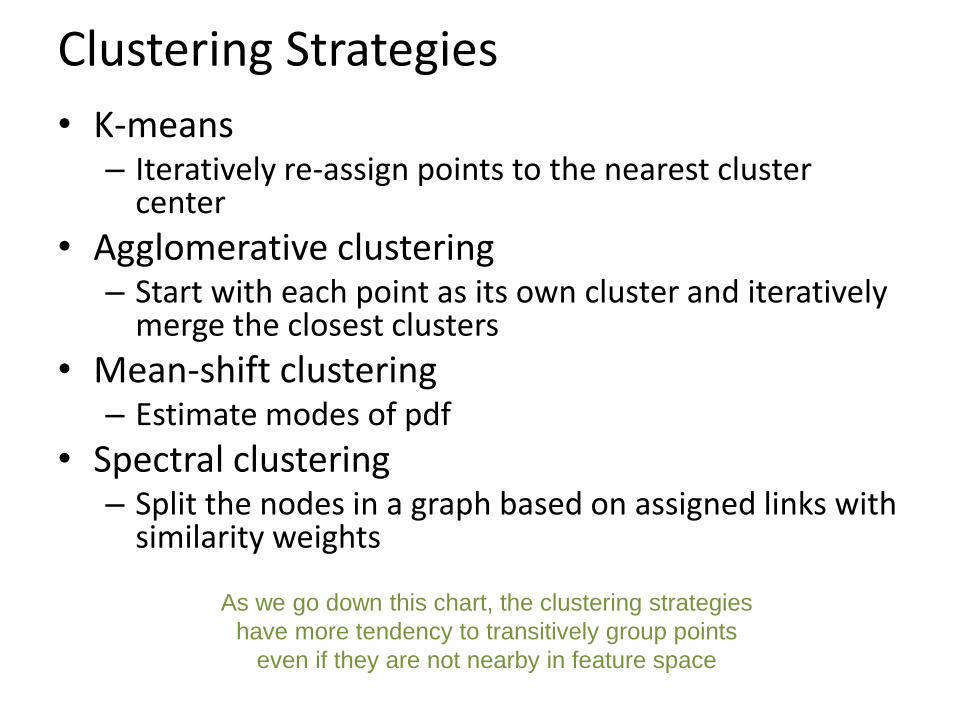
Clustering Strategies
• K-means – Iteratively re-assign points to the nearest cluster
center
• Agglomerative clustering – Start with each point as its own cluster and iteratively
merge the closest clusters
• Mean-shift clustering – Estimate modes of pdf
• Spectral clustering – Split the nodes in a graph based on assigned links with
similarity weights
As we go down this chart, the clustering strategies
have more tendency to transitively group points
even if they are not nearby in feature space
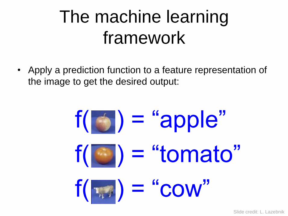
The machine learning
framework
• Apply a prediction function to a feature representation of
the image to get the desired output:
f( ) = “apple”
f( ) = “tomato”
f( ) = “cow”
Slide credit: L. Lazebnik
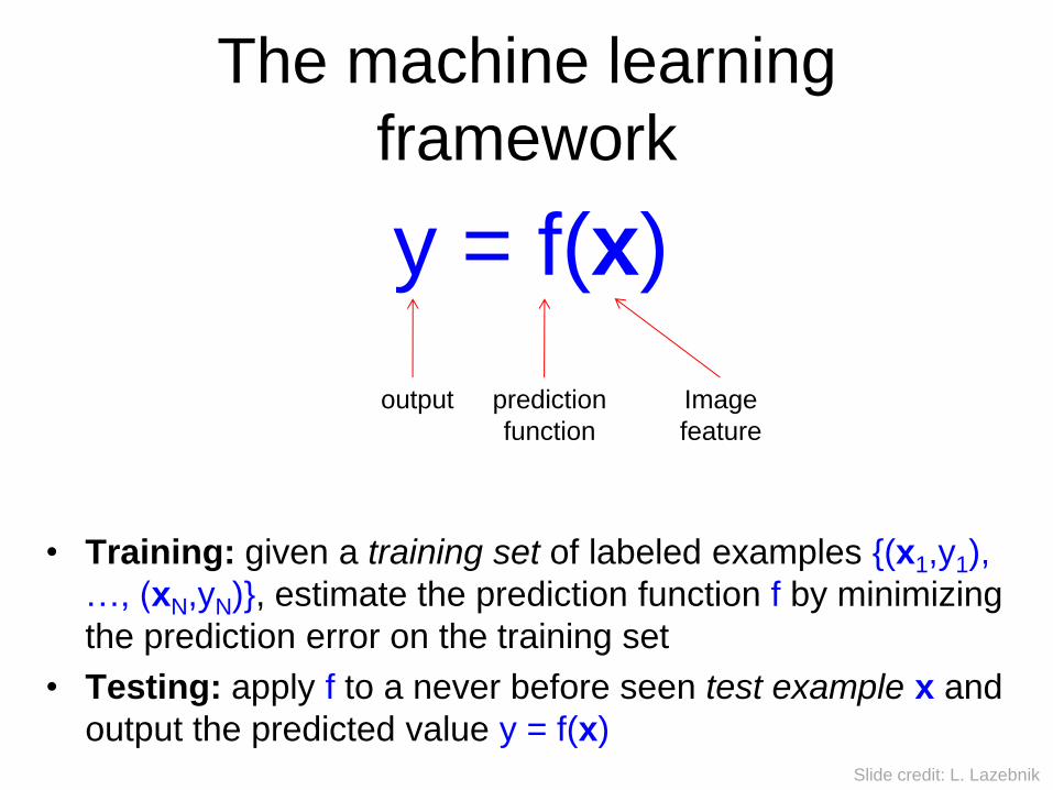
The machine learning
framework
y = f(x)
• Training: given a training set of labeled examples {(x1,y1),
…, (xN,yN)}, estimate the prediction function f by minimizing
the prediction error on the training set
• Testing: apply f to a never before seen test example x and
output the predicted value y = f(x)
output prediction
function
Image
feature
Slide credit: L. Lazebnik
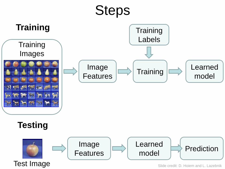
Prediction
Steps
Training
Labels Training
Images
Training
Training
Image
Features
Image
Features
Testing
Test Image
Learned
model
Learned
model
Slide credit: D. Hoiem and L. Lazebnik
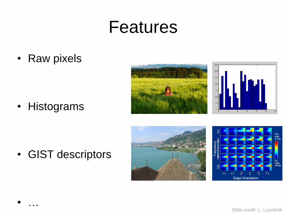
Features
• Raw pixels
• Histograms
• GIST descriptors
• … Slide credit: L. Lazebnik
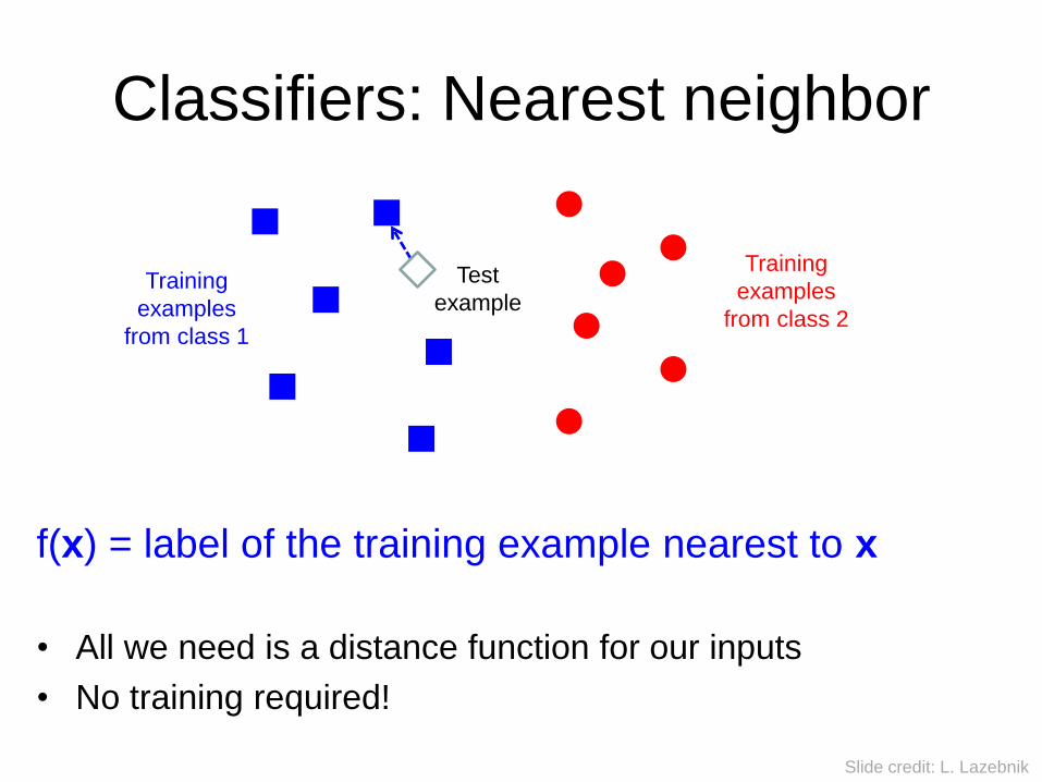
Classifiers: Nearest neighbor
f(x) = label of the training example nearest to x
• All we need is a distance function for our inputs
• No training required!
Test
example Training
examples
from class 1
Training
examples
from class 2
Slide credit: L. Lazebnik
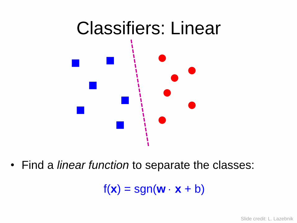
Classifiers: Linear
• Find a linear function to separate the classes:
f(x) = sgn(w x + b)
Slide credit: L. Lazebnik
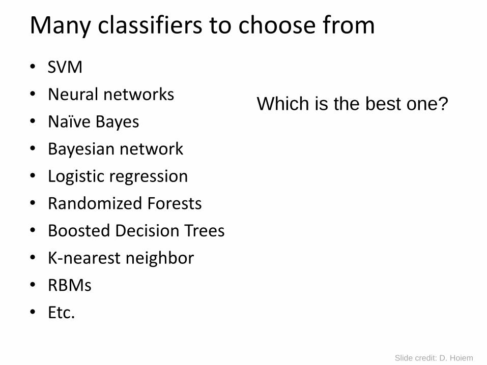
Many classifiers to choose from
• SVM
• Neural networks
• Naïve Bayes
• Bayesian network
• Logistic regression
• Randomized Forests
• Boosted Decision Trees
• K-nearest neighbor
• RBMs
• Etc.
Which is the best one?
Slide credit: D. Hoiem
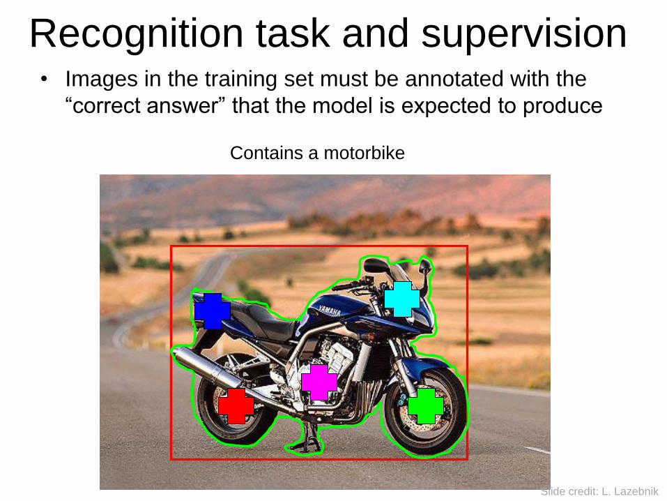
• Images in the training set must be annotated with the
“correct answer” that the model is expected to produce
Contains a motorbike
Recognition task and supervision
Slide credit: L. Lazebnik
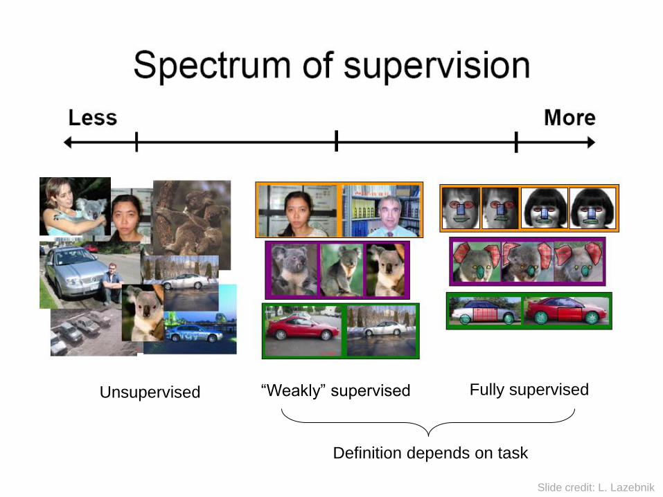
Unsupervised “Weakly” supervised Fully supervised
Definition depends on task
Slide credit: L. Lazebnik
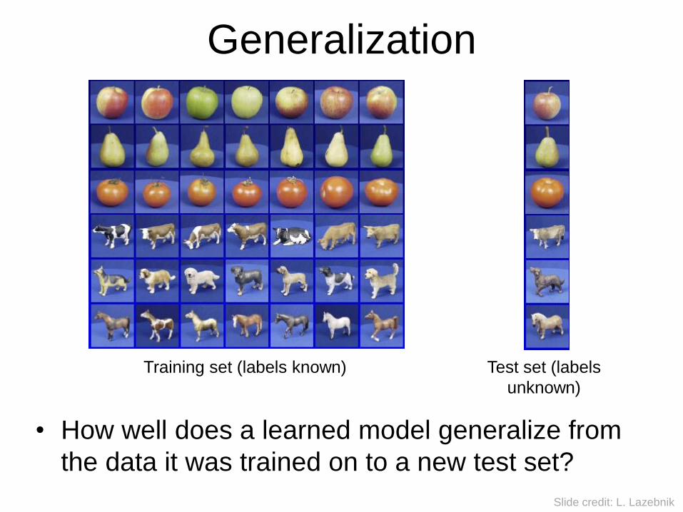
Generalization
• How well does a learned model generalize from
the data it was trained on to a new test set?
Training set (labels known) Test set (labels
unknown)
Slide credit: L. Lazebnik
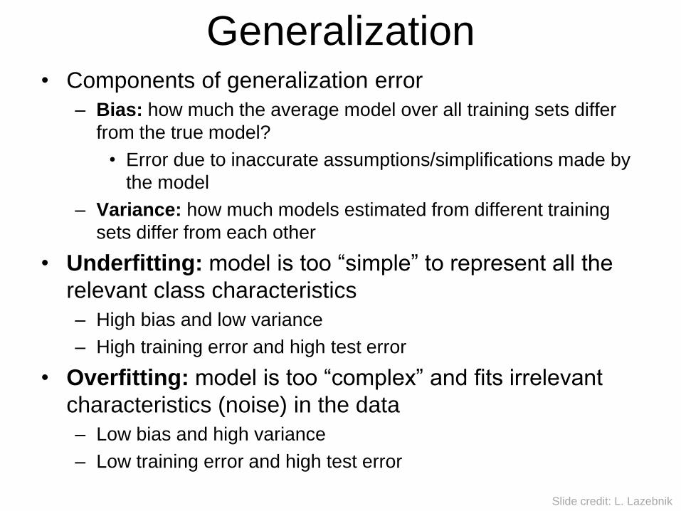
Generalization • Components of generalization error
– Bias: how much the average model over all training sets differ
from the true model?
• Error due to inaccurate assumptions/simplifications made by
the model
– Variance: how much models estimated from different training
sets differ from each other
• Underfitting: model is too “simple” to represent all the
relevant class characteristics
– High bias and low variance
– High training error and high test error
• Overfitting: model is too “complex” and fits irrelevant
characteristics (noise) in the data
– Low bias and high variance
– Low training error and high test error
Slide credit: L. Lazebnik
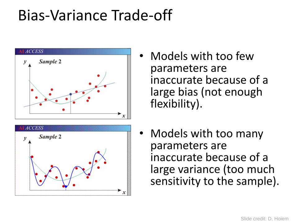
Bias-Variance Trade-off
• Models with too few parameters are inaccurate because of a large bias (not enough flexibility).
• Models with too many parameters are inaccurate because of a large variance (too much sensitivity to the sample).
Slide credit: D. Hoiem
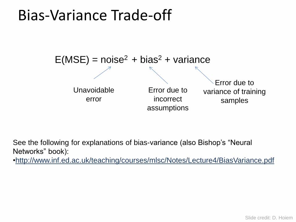
Bias-Variance Trade-off
E(MSE) = noise2 + bias2 + variance
See the following for explanations of bias-variance (also Bishop’s “Neural
Networks” book):
•http://www.inf.ed.ac.uk/teaching/courses/mlsc/Notes/Lecture4/BiasVariance.pdf
Unavoidable
error
Error due to
incorrect
assumptions
Error due to
variance of training
samples
Slide credit: D. Hoiem
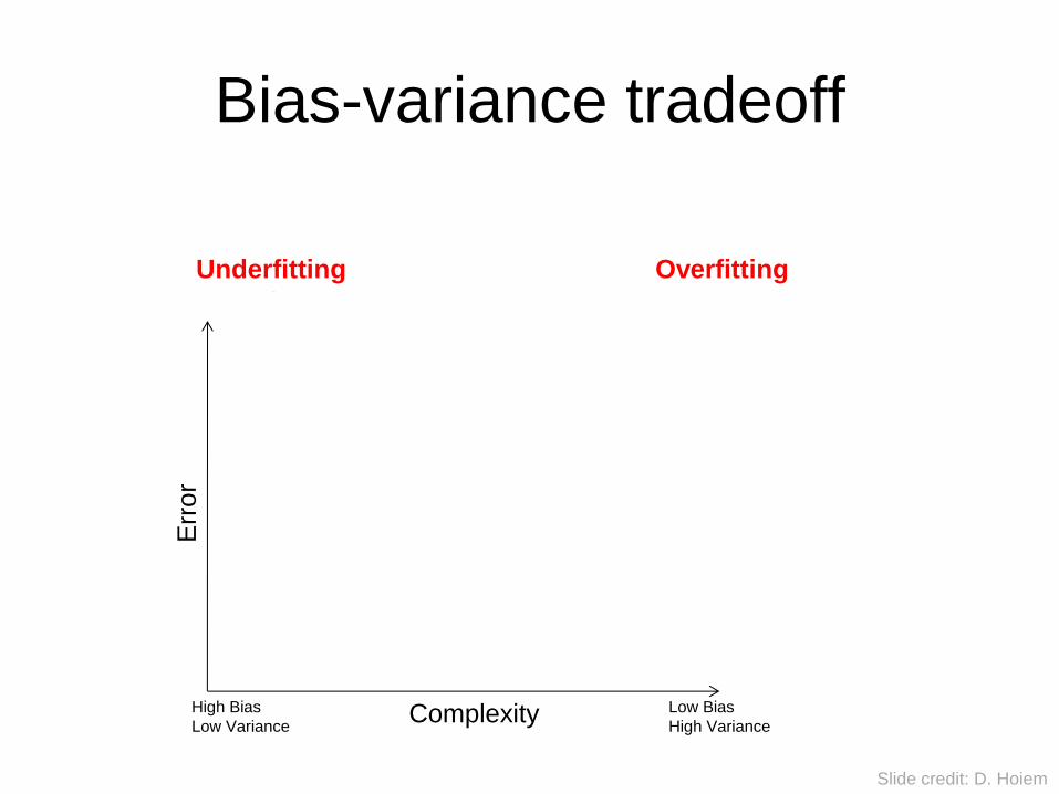
Bias-variance tradeoff
Training error
Test error
Underfitting Overfitting
Complexity Low Bias
High Variance
High Bias
Low Variance
Err
or
Slide credit: D. Hoiem
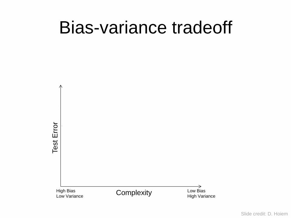
Bias-variance tradeoff
Many training examples
Few training examples
Complexity Low Bias
High Variance
High Bias
Low Variance
Test E
rror
Slide credit: D. Hoiem
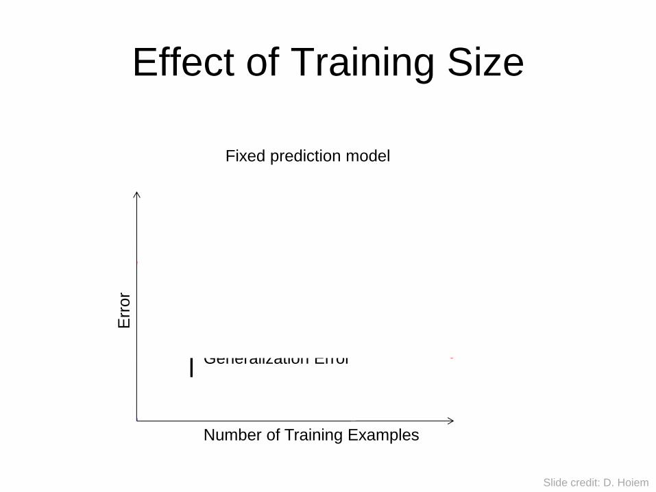
Effect of Training Size
Testing
Training
Generalization Error
Number of Training Examples
Err
or
Fixed prediction model
Slide credit: D. Hoiem
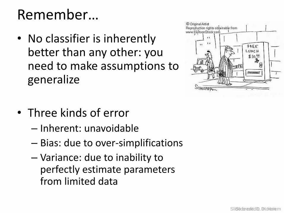
Remember…
• No classifier is inherently better than any other: you need to make assumptions to generalize
• Three kinds of error – Inherent: unavoidable
– Bias: due to over-simplifications
– Variance: due to inability to perfectly estimate parameters from limited data
Slide credit: D. Hoiem Slide credit: D. Hoiem
How to reduce variance?
• Choose a simpler classifier
• Regularize the parameters
• Get more training data
Slide credit: D. Hoiem
Very brief tour of some classifiers
• K-nearest neighbor
• SVM
• Boosted Decision Trees
• Neural networks
• Naïve Bayes
• Bayesian network
• Logistic regression
• Randomized Forests
• RBMs
• Etc.
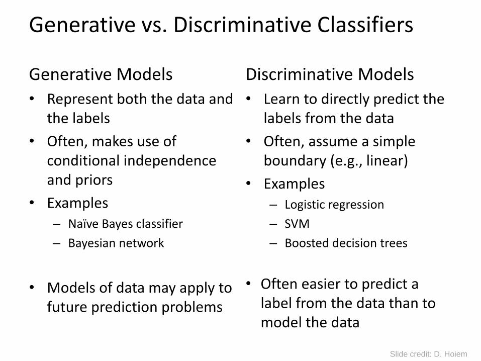
Generative vs. Discriminative Classifiers
Generative Models
• Represent both the data and the labels
• Often, makes use of conditional independence and priors
• Examples – Naïve Bayes classifier
– Bayesian network
• Models of data may apply to future prediction problems
Discriminative Models
• Learn to directly predict the labels from the data
• Often, assume a simple boundary (e.g., linear)
• Examples – Logistic regression
– SVM
– Boosted decision trees
• Often easier to predict a label from the data than to model the data
Slide credit: D. Hoiem
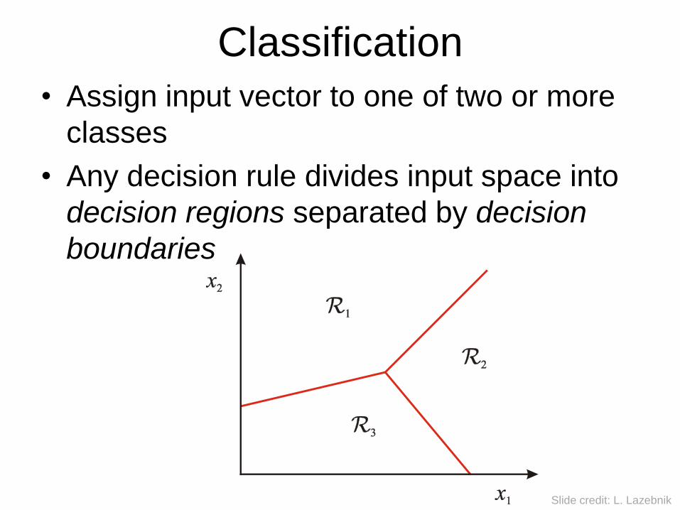
Classification
• Assign input vector to one of two or more
classes
• Any decision rule divides input space into
decision regions separated by decision
boundaries
Slide credit: L. Lazebnik

Nearest Neighbor Classifier
• Assign label of nearest training data point to each test data
point
Voronoi partitioning of feature space for two-category 2D and 3D data
from Duda et al.
Source: D. Lowe
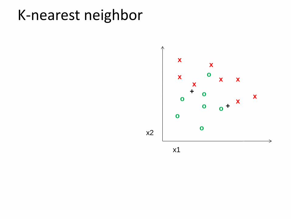
K-nearest neighbor
x x
x x
x
x
x
x
o
o o
o
o
o
o
x2
x1
+
+
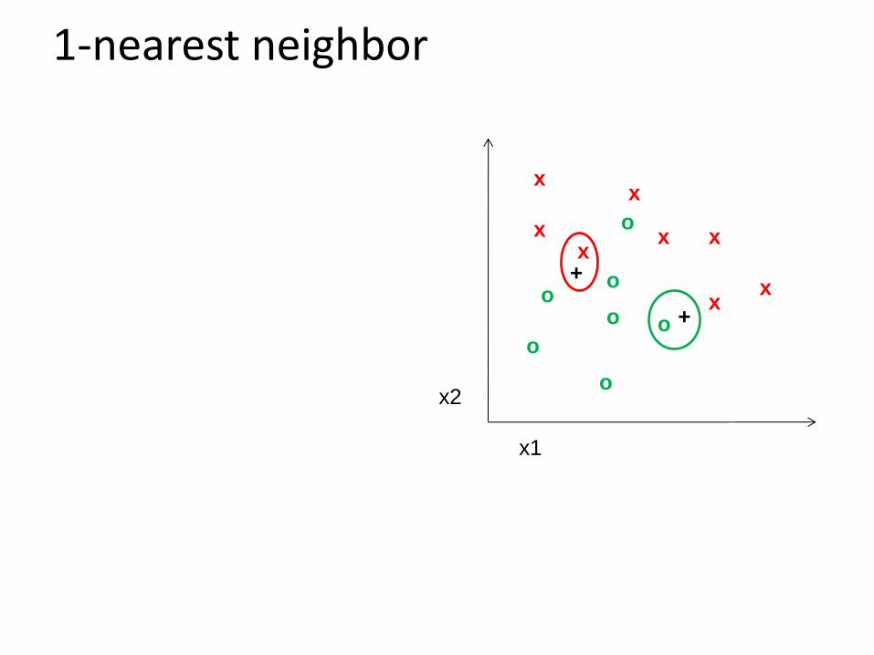
1-nearest neighbor
x x
x x
x
x
x
x
o
o o
o
o
o
o
x2
x1
+
+
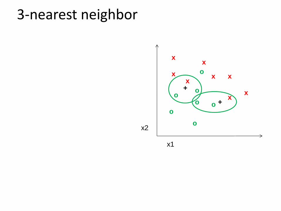
3-nearest neighbor
x x
x x
x
x
x
x
o
o o
o
o
o
o
x2
x1
+
+
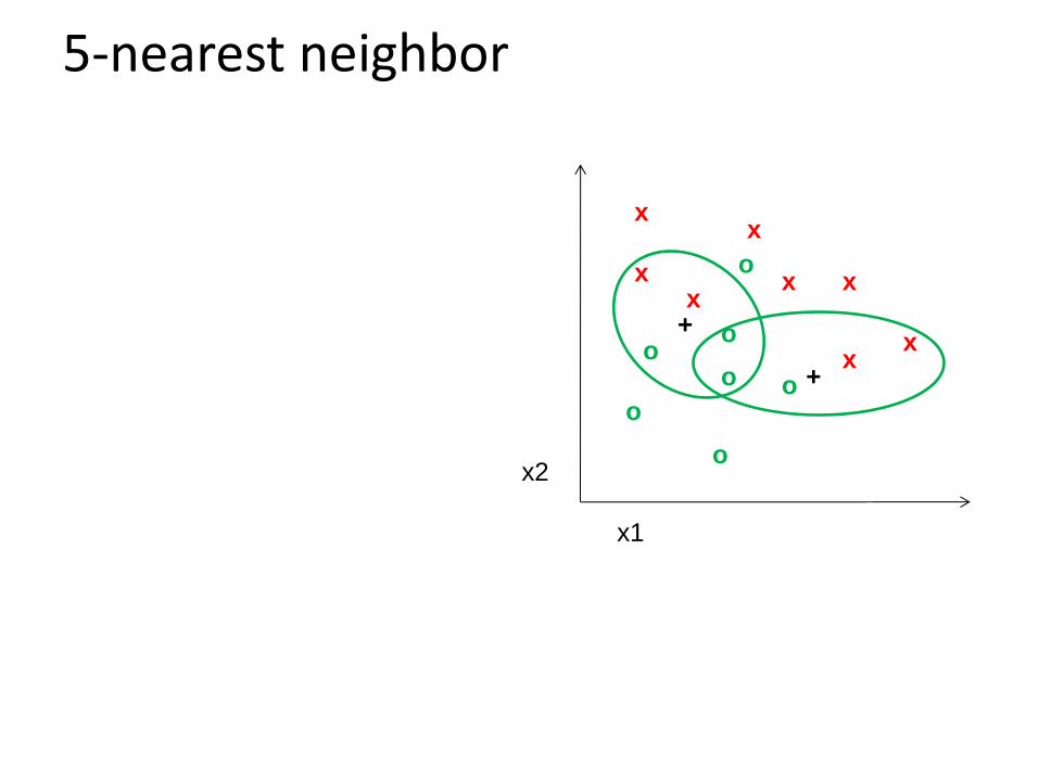
5-nearest neighbor
x x
x x
x
x
x
x
o
o o
o
o
o
o
x2
x1
+
+
Using K-NN
• Simple, a good one to try first
• With infinite examples, 1-NN provably has error that is at most twice Bayes optimal error
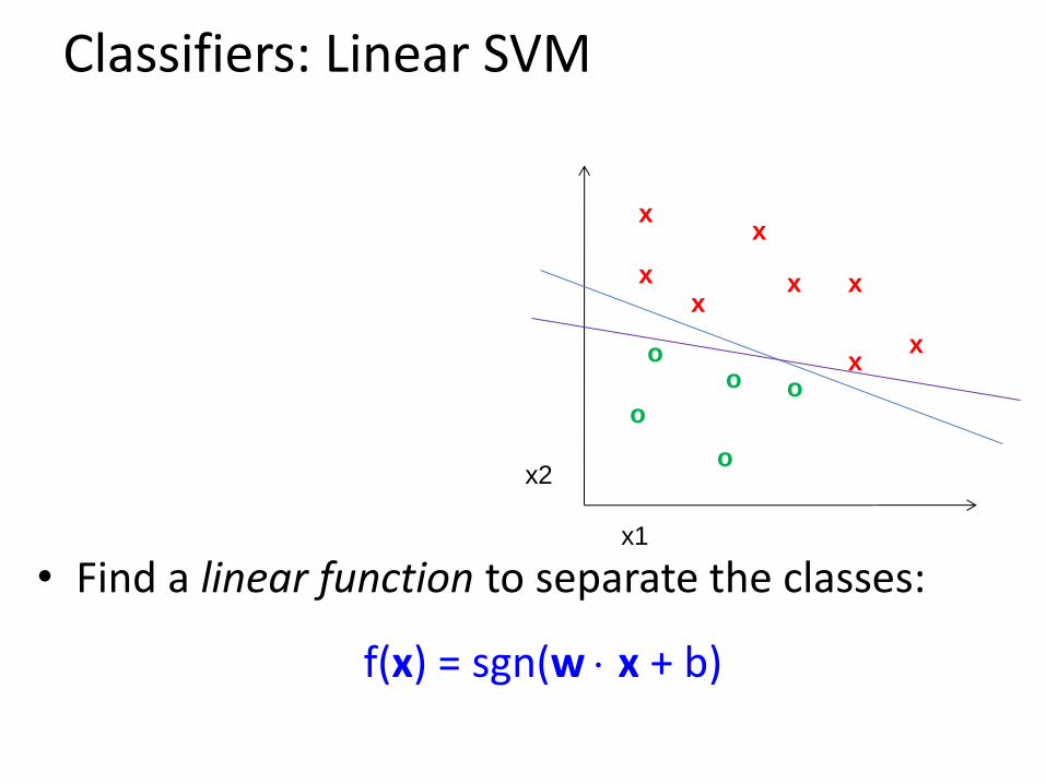
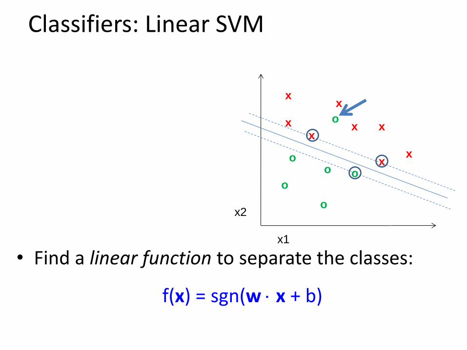
Classifiers: Linear SVM
x x
x x
x
x
x
x
o o
o
o
o
x2
x1
• Find a linear function to separate the classes:
f(x) = sgn(w x + b)

Classifiers: Linear SVM
x x
x x
x
x
x
x
o o
o
o
o
x2
x1
• Find a linear function to separate the classes:
f(x) = sgn(w x + b)
Classifiers: Linear SVM
x x
x x
x
x
x
x
o
o o
o
o
o
x2
x1
• Find a linear function to separate the classes:
f(x) = sgn(w x + b)
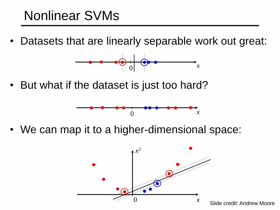
• Datasets that are linearly separable work out great:
• But what if the dataset is just too hard?
• We can map it to a higher-dimensional space:
0 x
0 x
0 x
x2
Nonlinear SVMs
Slide credit: Andrew Moore
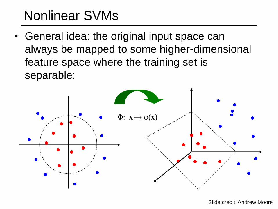
Φ: x → φ(x)
Nonlinear SVMs
• General idea: the original input space can
always be mapped to some higher-dimensional
feature space where the training set is
separable:
Slide credit: Andrew Moore
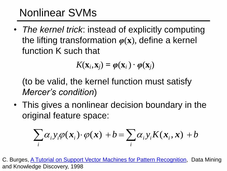
Nonlinear SVMs
• The kernel trick: instead of explicitly computing
the lifting transformation φ(x), define a kernel
function K such that
K(xi , xj) = φ(xi ) · φ(xj)
(to be valid, the kernel function must satisfy
Mercer’s condition)
• This gives a nonlinear decision boundary in the
original feature space:
bKybyi
iii
i
iii ),()()( xxxx
C. Burges, A Tutorial on Support Vector Machines for Pattern Recognition, Data Mining
and Knowledge Discovery, 1998
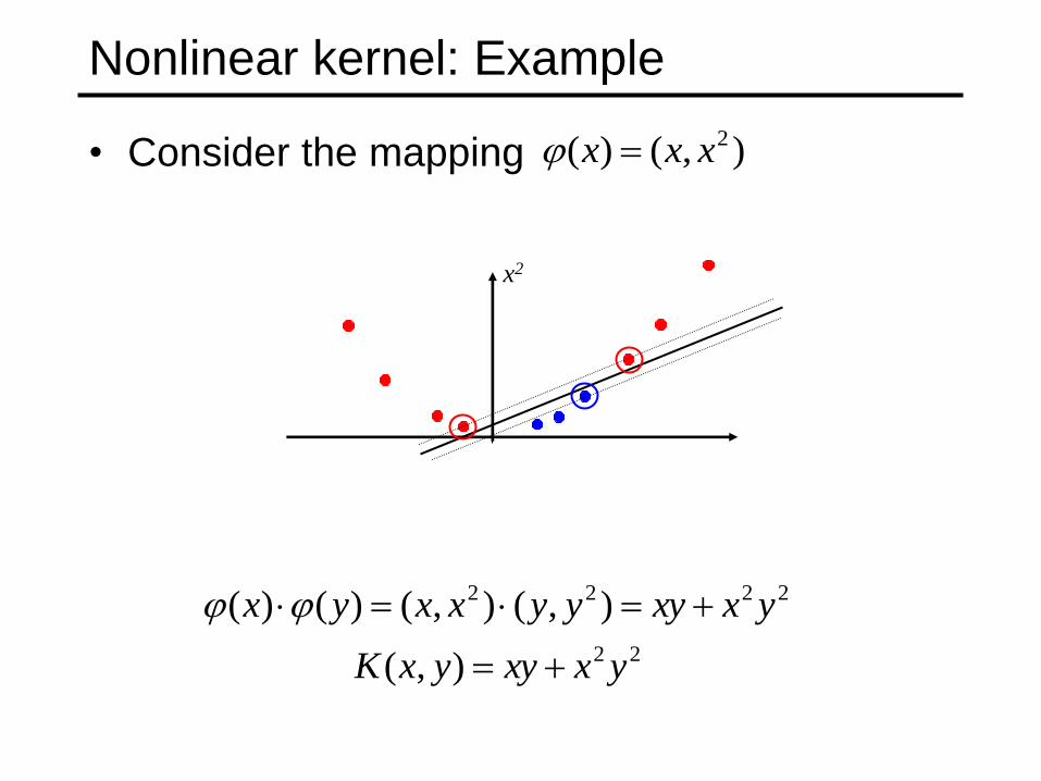
Nonlinear kernel: Example
• Consider the mapping ),()( 2xxx
22
2222
),(
),(),()()(
yxxyyxK
yxxyyyxxyx
x2
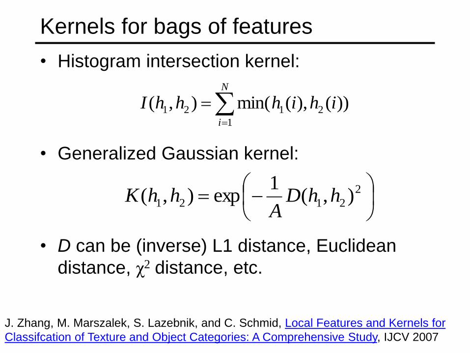
Kernels for bags of features
• Histogram intersection kernel:
• Generalized Gaussian kernel:
• D can be (inverse) L1 distance, Euclidean
distance, χ2 distance, etc.
N
i
ihihhhI1
2121 ))(),(min(),(
2
2121 ),(1
exp),( hhDA
hhK
J. Zhang, M. Marszalek, S. Lazebnik, and C. Schmid, Local Features and Kernels for
Classifcation of Texture and Object Categories: A Comprehensive Study, IJCV 2007
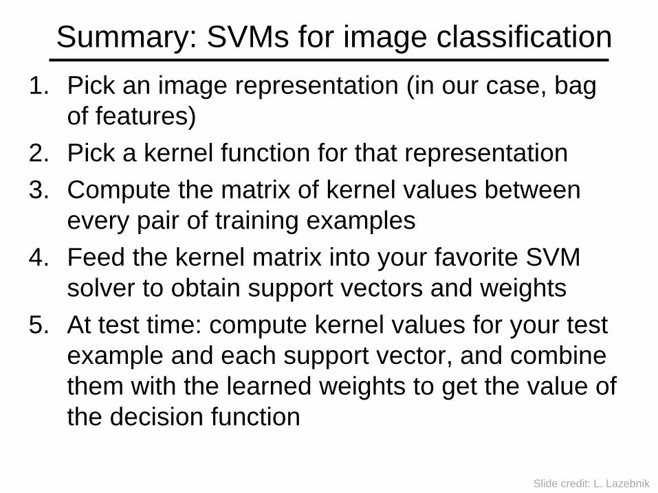
Summary: SVMs for image classification
1. Pick an image representation (in our case, bag
of features)
2. Pick a kernel function for that representation
3. Compute the matrix of kernel values between
every pair of training examples
4. Feed the kernel matrix into your favorite SVM
solver to obtain support vectors and weights
5. At test time: compute kernel values for your test
example and each support vector, and combine
them with the learned weights to get the value of
the decision function
Slide credit: L. Lazebnik

What about multi-class SVMs?
• Unfortunately, there is no “definitive” multi-
class SVM formulation
• In practice, we have to obtain a multi-class
SVM by combining multiple two-class SVMs
• One vs. others • Traning: learn an SVM for each class vs. the others
• Testing: apply each SVM to test example and assign to it the
class of the SVM that returns the highest decision value
• One vs. one • Training: learn an SVM for each pair of classes
• Testing: each learned SVM “votes” for a class to assign to
the test example
Slide credit: L. Lazebnik
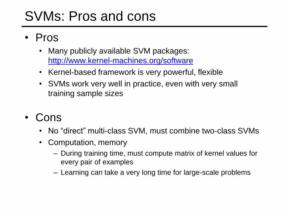
SVMs: Pros and cons
• Pros • Many publicly available SVM packages:
http://www.kernel-machines.org/software
• Kernel-based framework is very powerful, flexible
• SVMs work very well in practice, even with very small
training sample sizes
• Cons • No “direct” multi-class SVM, must combine two-class SVMs
• Computation, memory
– During training time, must compute matrix of kernel values for
every pair of examples
– Learning can take a very long time for large-scale problems
What to remember about classifiers
• No free lunch: machine learning algorithms are tools, not dogmas
• Try simple classifiers first
• Better to have smart features and simple classifiers than simple features and smart classifiers
• Use increasingly powerful classifiers with more training data (bias-variance tradeoff)
Slide credit: D. Hoiem
Some Machine Learning References
• General
– Tom Mitchell, Machine Learning, McGraw Hill, 1997
– Christopher Bishop, Neural Networks for Pattern Recognition, Oxford University Press, 1995
• Adaboost
– Friedman, Hastie, and Tibshirani, “Additive logistic regression: a statistical view of boosting”, Annals of Statistics, 2000
• SVMs
– http://www.support-vector.net/icml-tutorial.pdf
Slide credit: D. Hoiem