R and Data Mining: Examples and Case Studies 1

Yanchang Zhaoyanchang@rdatamining.com

http://www.RDataMining.com

April 26, 2013

1©2012-2013 Yanchang Zhao. Published by Elsevier in December 2012. All rights reserved.

Chapter 10

Text Mining

This chapter presents examples of text mining with R. Twitter1 text of @RDataMining is usedas the data to analyze. It starts with extracting text from Twitter. The extracted text is thentransformed to build a document-term matrix. After that, frequent words and associations arefound from the matrix. A word cloud is used to present important words in documents. In theend, words and tweets are clustered to find groups of words and also groups of tweets. In thischapter, “tweet” and “document” will be used interchangeably, so are “word” and “term”.

There are three important packages used in the examples: twitteR, tm and wordcloud . PackagetwitteR [Gentry, 2012] provides access to Twitter data, tm [Feinerer, 2012] provides functions fortext mining, and wordcloud [Fellows, 2012] visualizes the result with a word cloud 2.

10.1 Retrieving Text from Twitter

Twitter text is used in this chapter to demonstrate text mining. Tweets are extracted from Twitterwith the code below using userTimeline() in package twitteR [Gentry, 2012]. Package twitteRdepends on package RCurl [Lang, 2012a], which is available at http://www.stats.ox.ac.uk/

pub/RWin/bin/windows/contrib/. Another way to retrieve text from Twitter is using packageXML [Lang, 2012b], and an example on that is given at http://heuristically.wordpress.com/2011/04/08/text-data-mining-twitter-r/.

For readers who have no access to Twitter, the tweets data “rdmTweets.RData” can be down-loaded at http://www.rdatamining.com/data. Then readers can skip this section and proceeddirectly to Section 10.2.

Note that the Twitter API requires authentication since March 2013. Before running the codebelow, please complete authentication by following instructions in “Section 3: Authenticationwith OAuth” in the twitteR vignettes (http://cran.r-project.org/web/packages/twitteR/vignettes/twitteR.pdf).

> library(twitteR)

> # retrieve the first 200 tweets (or all tweets if fewer than 200) from the

> # user timeline of @rdatammining

> rdmTweets <- userTimeline("rdatamining", n=200)

> (nDocs <- length(rdmTweets))

[1] 154

Next, we have a look at the five tweets numbered 11 to 15.

> rdmTweets[11:15]

1http://www.twitter.com2http://en.wikipedia.org/wiki/Word_cloud

97

98 CHAPTER 10. TEXT MINING

With the above code, each tweet is printed in one single line, which may exceed the boundaryof paper. Therefore, the following code is used in this book to print the five tweets by wrappingthe text to fit the width of paper. The same method is used to print tweets in other codes in thischapter.

> for (i in 11:15) {

+ cat(paste("[[", i, "]] ", sep=""))

+ writeLines(strwrap(rdmTweets[[i]]$getText(), width=73))

+ }

[[11]] Slides on massive data, shared and distributed memory,and concurrent

programming: bigmemory and foreach http://t.co/a6bQzxj5

[[12]] The R Reference Card for Data Mining is updated with functions &

packages for handling big data & parallel computing.

http://t.co/FHoVZCyk

[[13]] Post-doc on Optimizing a Cloud for Data Mining primitives, INRIA, France

http://t.co/cA28STPO

[[14]] Chief Scientist - Data Intensive Analytics, Pacific Northwest National

Laboratory (PNNL), US http://t.co/0Gdzq1Nt

[[15]] Top 10 in Data Mining http://t.co/7kAuNvuf

10.2 Transforming Text

The tweets are first converted to a data frame and then to a corpus, which is a collection oftext documents. After that, the corpus can be processed with functions provided in packagetm [Feinerer, 2012].

> # convert tweets to a data frame

> df <- do.call("rbind", lapply(rdmTweets, as.data.frame))

> dim(df)

[1] 154 10

> library(tm)

> # build a corpus, and specify the source to be character vectors

> myCorpus <- Corpus(VectorSource(df$text))

After that, the corpus needs a couple of transformations, including changing letters to lowercase, and removing punctuations, numbers and stop words. The general English stop-word list istailored here by adding “available” and “via” and removing “r” and “big” (for big data). Hyperlinksare also removed in the example below.

> # convert to lower case

> myCorpus <- tm_map(myCorpus, tolower)

> # remove punctuation

> myCorpus <- tm_map(myCorpus, removePunctuation)

> # remove numbers

> myCorpus <- tm_map(myCorpus, removeNumbers)

> # remove URLs

> removeURL <- function(x) gsub("http[[:alnum:]]*", "", x)

> myCorpus <- tm_map(myCorpus, removeURL)

> # add two extra stop words: "available" and "via"

> myStopwords <- c(stopwords('english'), "available", "via")

> # remove "r" and "big" from stopwords

> myStopwords <- setdiff(myStopwords, c("r", "big"))

> # remove stopwords from corpus

> myCorpus <- tm_map(myCorpus, removeWords, myStopwords)

10.3. STEMMING WORDS 99

In the above code, tm_map() is an interface to apply transformations (mappings) to corpora. Alist of available transformations can be obtained with getTransformations(), and the mostly usedones are as.PlainTextDocument(), removeNumbers(), removePunctuation(), removeWords(),stemDocument() and stripWhitespace(). A function removeURL() is defined above to removehypelinks, where pattern "http[[:alnum:]]*" matches strings starting with “http” and thenfollowed by any number of alphabetic characters and digits. Strings matching this pattern areremoved with gsub(). The above pattern is specified as an regular expression, and detail aboutthat can be found by running ?regex in R.

10.3 Stemming Words

In many applications, words need to be stemmed to retrieve their radicals, so that various formsderived from a stem would be taken as the same when counting word frequency. For instance,words “update”, “updated” and “updating” would all be stemmed to “updat”. Word stemmingcan be done with the snowball stemmer, which requires packages Snowball , RWeka, rJava andRWekajars. After that, we can complete the stems to their original forms, i.e., “update” forthe above example, so that the words would look normal. This can be achieved with functionstemCompletion().

> # keep a copy of corpus to use later as a dictionary for stem completion

> myCorpusCopy <- myCorpus

> # stem words

> myCorpus <- tm_map(myCorpus, stemDocument)

> # inspect documents (tweets) numbered 11 to 15

> # inspect(myCorpus[11:15])

> # The code below is used for to make text fit for paper width

> for (i in 11:15) {

+ cat(paste("[[", i, "]] ", sep=""))

+ writeLines(strwrap(myCorpus[[i]], width=73))

+ }

[[11]] slide massiv data share distribut memoryand concurr program bigmemori

foreach

[[12]] r refer card data mine updat function packag handl big data parallel

comput

[[13]] postdoc optim cloud data mine primit inria franc

[[14]] chief scientist data intens analyt pacif northwest nation laboratori

pnnl

[[15]] top data mine

After that, we use stemCompletion() to complete the stems with the unstemmed corpusmyCorpusCopy as a dictionary. With the default setting, it takes the most frequent match indictionary as completion.

> # stem completion

> myCorpus <- tm_map(myCorpus, stemCompletion, dictionary=myCorpusCopy)

Then we have a look at the documents numbered 11 to 15 in the built corpus.

> inspect(myCorpus[11:15])

[[11]] slides massive data share distributed memoryand concurrent programming

foreach

[[12]] r reference card data miners updated functions package handling big data

parallel computing

100 CHAPTER 10. TEXT MINING

[[13]] postdoctoral optimizing cloud data miners primitives inria france

[[14]] chief scientist data intensive analytics pacific northwest national pnnl

[[15]] top data miners

As we can see from the above results, there are something unexpected in the above stemmingand completion.

1. In both the stemmed corpus and the completed one, “memoryand” is derived from “... mem-ory,and ...” in the original tweet 11.

2. In tweet 11, word “bigmemory” is stemmed to “bigmemori”, and then is removed during stemcompletion.

3. Word “mining” in tweets 12, 13 & 15 is first stemmed to “mine” and then completed to“miners”.

4. “Laboratory” in tweet 14 is stemmed to “laboratori” and then also disappears after comple-tion.

In the above issues, point 1 is caused by the missing of a space after the comma. It can beeasily fixed by replacing comma with space before removing punctuation marks in Section 10.2.For points 2 & 4, we haven’t figured out why it happened like that. Fortunately, the words involvedin points 1, 2 & 4 are not important in @RDataMining tweets and ignoring them would not bringany harm to this demonstration of text mining.

Below we focus on point 3, where word “mining” is first stemmed to “mine” and then completedto “miners”, instead of “mining”, although there are many instances of “mining” in the tweets,compared to only two instances of “miners”. There might be a solution for the above problem bychanging the parameters and/or dictionaries for stemming and completion, but we failed to findone due to limitation of time and efforts. Instead, we chose a simple way to get around of thatby replacing “miners” with “mining”, since the latter has many more cases than the former in thecorpus. The code for the replacement is given below.

> # count frequency of "mining"

> miningCases <- tm_map(myCorpusCopy, grep, pattern="\\<mining")

> sum(unlist(miningCases))

[1] 47

> # count frequency of "miners"

> minerCases <- tm_map(myCorpusCopy, grep, pattern="\\<miners")

> sum(unlist(minerCases))

[1] 2

> # replace "miners" with "mining"

> myCorpus <- tm_map(myCorpus, gsub, pattern="miners", replacement="mining")

In the first call of function tm_map() in the above code, grep() is applied to every document(tweet) with argument “pattern="\\<mining"”. The pattern matches words starting with “min-ing”, where “\<” matches the empty string at the beginning of a word. This ensures that text“rdatamining” would not contribute to the above counting of “mining”.

10.4 Building a Term-Document Matrix

A term-document matrix represents the relationship between terms and documents, where eachrow stands for a term and each column for a document, and an entry is the number of occurrences of

10.5. FREQUENT TERMS AND ASSOCIATIONS 101

the term in the document. Alternatively, one can also build a document-term matrix by swappingrow and column. In this section, we build a term-document matrix from the above processedcorpus with function TermDocumentMatrix(). With its default setting, terms with less than threecharacters are discarded. To keep “r” in the matrix, we set the range of wordLengths in theexample below.

> myTdm <- TermDocumentMatrix(myCorpus, control=list(wordLengths=c(1,Inf)))

> myTdm

A term-document matrix (444 terms, 154 documents)

Non-/sparse entries: 1085/67291

Sparsity : 98%

Maximal term length: 27

Weighting : term frequency (tf)

As we can see from the above result, the term-document matrix is composed of 444 terms and154 documents. It is very sparse, with 98% of the entries being zero. We then have a look at thefirst six terms starting with “r” and tweets numbered 101 to 110.

> idx <- which(dimnames(myTdm)$Terms == "r")

> inspect(myTdm[idx+(0:5),101:110])

A term-document matrix (6 terms, 10 documents)

Non-/sparse entries: 9/51

Sparsity : 85%

Maximal term length: 12

Weighting : term frequency (tf)

Docs

Terms 101 102 103 104 105 106 107 108 109 110

r 1 1 0 0 2 0 0 1 1 1

ramachandran 0 0 0 0 0 0 0 0 0 0

random 0 0 0 0 0 0 0 0 0 0

ranked 0 0 0 0 0 0 0 0 1 0

rapidminer 1 0 0 0 0 0 0 0 0 0

rdatamining 0 0 0 0 0 0 0 1 0 0

Note that the parameter to control word length used to be minWordLength prior to version0.5-7 of package tm. The code to set the minimum word length for old versions of tm is below.

> myTdm <- TermDocumentMatrix(myCorpus, control=list(minWordLength=1))

The list of terms can be retrieved with rownames(myTdm). Based on the above matrix, manydata mining tasks can be done, for example, clustering, classification and association analysis.

When there are too many terms, the size of a term-document matrix can be reduced byselecting terms that appear in a minimum number of documents, or filtering terms with TF-IDF(term frequency-inverse document frequency) [Wu et al., 2008].

10.5 Frequent Terms and Associations

We have a look at the popular words and the association between words. Note that there are 154tweets in total.

> # inspect frequent words

> findFreqTerms(myTdm, lowfreq=10)

102 CHAPTER 10. TEXT MINING

[1] "analysis" "computing" "data" "examples" "introduction"

[6] "mining" "network" "package" "positions" "postdoctoral"

[11] "r" "research" "slides" "social" "tutorial"

[16] "users"

In the code above, findFreqTerms() finds frequent terms with frequency no less than ten.Note that they are ordered alphabetically, instead of by frequency or popularity.

To show the top frequent words visually, we next make a barplot for them. From the term-document matrix, we can derive the frequency of terms with rowSums(). Then we select terms thatappears in ten or more documents and shown them with a barplot using package ggplot2 [Wickham,2009]. In the code below, geom="bar" specifies a barplot and coord_flip() swaps x- and y-axis.The barplot in Figure 10.1 clearly shows that the three most frequent words are “r”, “data” and“mining”.

> termFrequency <- rowSums(as.matrix(myTdm))

> termFrequency <- subset(termFrequency, termFrequency>=10)

> library(ggplot2)

> qplot(names(termFrequency), termFrequency, geom="bar", xlab="Terms") + coord_flip()

analysis

computing

data

examples

introduction

mining

network

package

positions

postdoctoral

r

research

slides

social

tutorial

users

0 20 40 60 80termFrequency

Term

s

Figure 10.1: Frequent Terms

Alternatively, the above plot can also be drawn with barplot() as below, where las sets thedirection of x-axis labels to be vertical.

> barplot(termFrequency, las=2)

We can also find what are highly associated with a word with function findAssocs(). Belowwe try to find terms associated with “r” (or “mining”) with correlation no less than 0.25, and thewords are ordered by their correlation with “r” (or “mining”).

> # which words are associated with "r"?

> findAssocs(myTdm, 'r', 0.25)

10.6. WORD CLOUD 103

users canberra cran list examples

0.32 0.26 0.26 0.26 0.25

> # which words are associated with "mining"?

> findAssocs(myTdm, 'mining', 0.25)

data mahout recommendation sets supports

0.55 0.39 0.39 0.39 0.39

frequent itemset card functions reference

0.35 0.34 0.29 0.29 0.29

text

0.26

10.6 Word Cloud

After building a term-document matrix, we can show the importance of words with a word cloud(also known as a tag cloud), which can be easily produced with package wordcloud [Fellows,2012]. In the code below, we first convert the term-document matrix to a normal matrix, andthen calculate word frequencies. After that, we set gray levels based on word frequency and usewordcloud() to make a plot for it. With wordcloud(), the first two parameters give a list ofwords and their frequencies. Words with frequency below three are not plotted, as specified bymin.freq=3. By setting random.order=F, frequent words are plotted first, which makes themappear in the center of cloud. We also set the colors to gray levels based on frequency. A colorfulcloud can be generated by setting colors with rainbow().

> library(wordcloud)

> m <- as.matrix(myTdm)

> # calculate the frequency of words and sort it descendingly by frequency

> wordFreq <- sort(rowSums(m), decreasing=TRUE)

> # word cloud

> set.seed(375) # to make it reproducible

> grayLevels <- gray( (wordFreq+10) / (max(wordFreq)+10) )

> wordcloud(words=names(wordFreq), freq=wordFreq, min.freq=3, random.order=F,

+ colors=grayLevels)

104 CHAPTER 10. TEXT MINING

rdata

mininganalysis

packageusersexamplesnetwork

tutorial

slides

rese

arch

social

positionspostdoctoral

computingin

trod

uctio

n

applicationscode

clusteringparallel

series

time

graphics

pdf

statistics

talk

text

free

learn

advanced

australiacard

dete

ctio

n

functions

info

rmat

ion

lecture

modelling

rdatamining

reference

scie

ntis

t

spatial

techniquestoolsuniversity

analyst

book

clas

sific

atio

n

datasets

distributed

expe

rienc

e fast

frequent

job

join

outlier

performance

programmingsnowfall

tried

twitter

vacancy

websitewwwrdataminingcom

access

analyticsanswers

association

big

charts

china

com

men

ts

databases

details

documents

followed

itemset

melbourne

notes

poll

presentations

processing

publ

ishe

d

recentshort

technology

viewsvisits

visualizing

Figure 10.2: Word Cloud

The above word cloud clearly shows again that “r”, “data” and “mining” are the top threewords, which validates that the @RDataMining tweets present information on R and data mining.Some other important words are “analysis”, “examples”, “slides”, “tutorial” and “package”, whichshows that it focuses on documents and examples on analysis and R packages. Another set offrequent words, “research”, “postdoctoral” and “positions”, are from tweets about vacancies onpost-doctoral and research positions. There are also some tweets on the topic of social networkanalysis, as indicated by words “network” and “social” in the cloud.

10.7 Clustering Words

We then try to find clusters of words with hierarchical clustering. Sparse terms are removed, sothat the plot of clustering will not be crowded with words. Then the distances between terms arecalculated with dist() after scaling. After that, the terms are clustered with hclust() and thedendrogram is cut into 10 clusters. The agglomeration method is set to ward, which denotes theincrease in variance when two clusters are merged. Some other options are single linkage, completelinkage, average linkage, median and centroid. Details about different agglomeration methods canbe found in data mining textbooks [Han and Kamber, 2000,Hand et al., 2001,Witten and Frank,2005].

> # remove sparse terms

> myTdm2 <- removeSparseTerms(myTdm, sparse=0.95)

> m2 <- as.matrix(myTdm2)

> # cluster terms

10.8. CLUSTERING TWEETS 105

> distMatrix <- dist(scale(m2))

> fit <- hclust(distMatrix, method="ward")

> plot(fit)

> # cut tree into 10 clusters

> rect.hclust(fit, k=10)

> (groups <- cutree(fit, k=10))

analysis applications code computing data examples

1 2 3 4 5 3

introduction mining network package parallel positions

2 6 1 7 4 8

postdoctoral r research series slides social

8 9 8 10 2 1

time tutorial users

10 2 2

anal

ysis

netw

ork

soci

al

posi

tions

post

doct

oral

rese

arch

serie

s

time

pack

age

com

putin

g

para

llel co

de

exam

ples

tuto

rial

slid

es

appl

icat

ions

intr

oduc

tion

user

s

r

data

min

ing

010

2030

4050

Cluster Dendrogram

hclust (*, "ward")distMatrix

Hei

ght

Figure 10.3: Clustering of Words

In the above dendrogram, we can see the topics in the tweets. Words “analysis”, “network”and “social” are clustered into one group, because there are a couple of tweets on social networkanalysis. The second cluster from left comprises “positions”, “postdoctoral” and “research”, andthey are clustered into one group because of tweets on vacancies of research and postdoctoralpositions. We can also see cluster on time series, R packages, parallel computing, R codes andexamples, and tutorial and slides. The rightmost three clusters consists of“r”, “data”and“mining”,which are the keywords of @RDataMining tweets.

10.8 Clustering Tweets

Tweets are clustered below with the k-means and the k-medoids algorithms.

106 CHAPTER 10. TEXT MINING

10.8.1 Clustering Tweets with the k-means Algorithm

We first try k-means clustering, which takes the values in the matrix as numeric. We transposethe term-document matrix to a document-term one. The tweets are then clustered with kmeans()

with the number of clusters set to eight. After that, we check the popular words in every clusterand also the cluster centers. Note that a fixed random seed is set with set.seed() before runningkmeans(), so that the clustering result can be reproduced. It is for the convenience of book writing,and it is unnecessary for readers to set a random seed in their code.

> # transpose the matrix to cluster documents (tweets)

> m3 <- t(m2)

> # set a fixed random seed

> set.seed(122)

> # k-means clustering of tweets

> k <- 8

> kmeansResult <- kmeans(m3, k)

> # cluster centers

> round(kmeansResult$centers, digits=3)

analysis applications code computing data examples introduction mining network

1 0.040 0.040 0.240 0.000 0.040 0.320 0.040 0.120 0.080

2 0.000 0.158 0.053 0.053 1.526 0.105 0.053 1.158 0.000

3 0.857 0.000 0.000 0.000 0.000 0.071 0.143 0.071 1.000

4 0.000 0.000 0.000 1.000 0.000 0.000 0.000 0.000 0.000

5 0.037 0.074 0.019 0.019 0.426 0.037 0.093 0.407 0.000

6 0.000 0.000 0.000 0.000 0.000 0.100 0.000 0.000 0.000

7 0.533 0.000 0.067 0.000 0.333 0.200 0.067 0.200 0.067

8 0.000 0.111 0.000 0.000 0.556 0.000 0.000 0.111 0.000

package parallel positions postdoctoral r research series slides social

1 0.080 0.000 0.000 0.000 1.320 0.000 0.040 0.000 0.000

2 0.368 0.053 0.000 0.000 0.947 0.053 0.000 0.053 0.000

3 0.071 0.000 0.143 0.143 0.214 0.071 0.000 0.071 0.786

4 0.125 0.750 0.000 0.000 1.000 0.000 0.000 0.125 0.000

5 0.000 0.000 0.093 0.093 0.000 0.000 0.019 0.074 0.000

6 1.200 0.100 0.000 0.000 0.600 0.100 0.000 0.100 0.000

7 0.000 0.000 0.000 0.000 1.000 0.000 0.400 0.533 0.000

8 0.000 0.000 0.444 0.444 0.000 1.333 0.000 0.000 0.111

time tutorial users

1 0.040 0.200 0.160

2 0.000 0.000 0.158

3 0.000 0.286 0.071

4 0.000 0.125 0.250

5 0.019 0.111 0.019

6 0.000 0.100 0.100

7 0.400 0.000 0.400

8 0.000 0.000 0.000

To make it easy to find what the clusters are about, we then check the top three words in everycluster.

> for (i in 1:k) {

+ cat(paste("cluster ", i, ": ", sep=""))

+ s <- sort(kmeansResult$centers[i,], decreasing=T)

+ cat(names(s)[1:3], "\n")

+ # print the tweets of every cluster

10.8. CLUSTERING TWEETS 107

+ # print(rdmTweets[which(kmeansResult$cluster==i)])

+ }

cluster 1: r examples code

cluster 2: data mining r

cluster 3: network analysis social

cluster 4: computing r parallel

cluster 5: data mining tutorial

cluster 6: package r examples

cluster 7: r analysis slides

cluster 8: research data positions

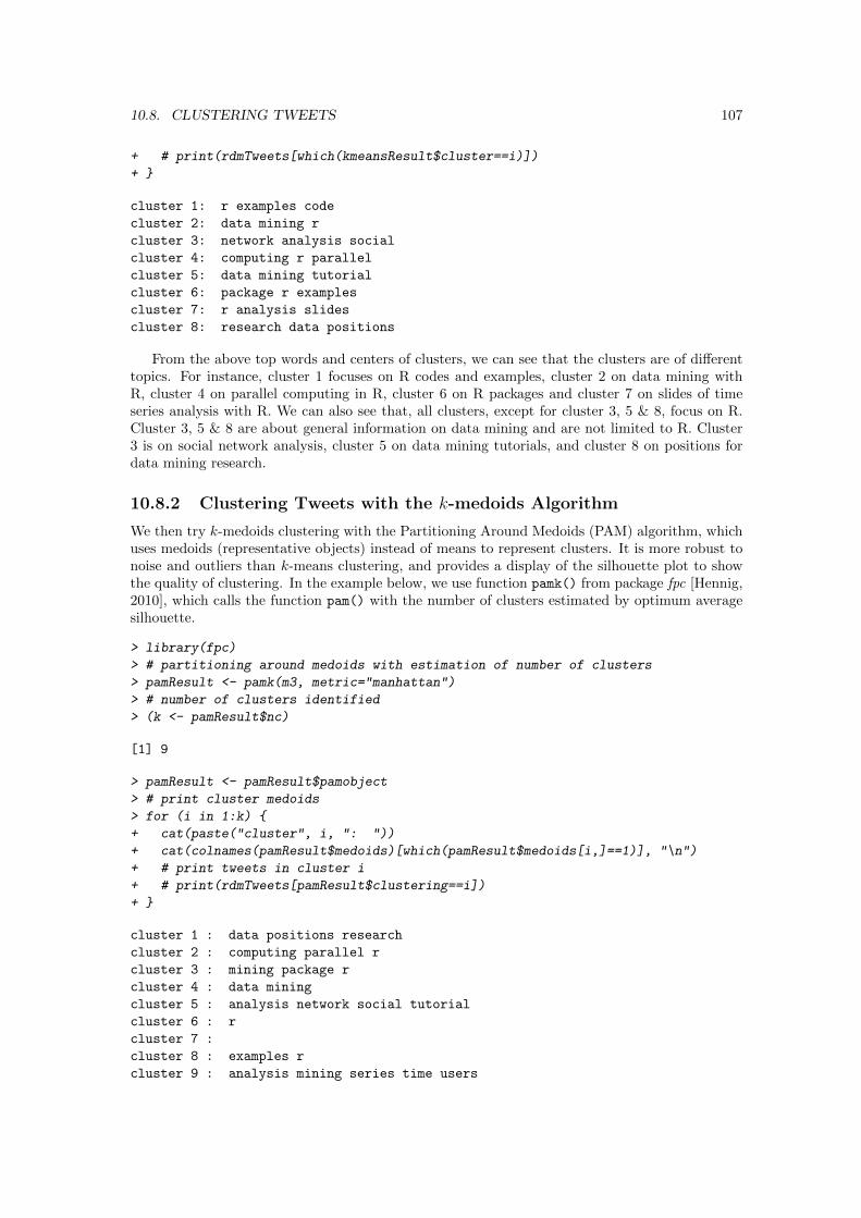
From the above top words and centers of clusters, we can see that the clusters are of differenttopics. For instance, cluster 1 focuses on R codes and examples, cluster 2 on data mining withR, cluster 4 on parallel computing in R, cluster 6 on R packages and cluster 7 on slides of timeseries analysis with R. We can also see that, all clusters, except for cluster 3, 5 & 8, focus on R.Cluster 3, 5 & 8 are about general information on data mining and are not limited to R. Cluster3 is on social network analysis, cluster 5 on data mining tutorials, and cluster 8 on positions fordata mining research.

10.8.2 Clustering Tweets with the k-medoids Algorithm

We then try k-medoids clustering with the Partitioning Around Medoids (PAM) algorithm, whichuses medoids (representative objects) instead of means to represent clusters. It is more robust tonoise and outliers than k-means clustering, and provides a display of the silhouette plot to showthe quality of clustering. In the example below, we use function pamk() from package fpc [Hennig,2010], which calls the function pam() with the number of clusters estimated by optimum averagesilhouette.

> library(fpc)

> # partitioning around medoids with estimation of number of clusters

> pamResult <- pamk(m3, metric="manhattan")

> # number of clusters identified

> (k <- pamResult$nc)

[1] 9

> pamResult <- pamResult$pamobject

> # print cluster medoids

> for (i in 1:k) {

+ cat(paste("cluster", i, ": "))

+ cat(colnames(pamResult$medoids)[which(pamResult$medoids[i,]==1)], "\n")

+ # print tweets in cluster i

+ # print(rdmTweets[pamResult$clustering==i])

+ }

cluster 1 : data positions research

cluster 2 : computing parallel r

cluster 3 : mining package r

cluster 4 : data mining

cluster 5 : analysis network social tutorial

cluster 6 : r

cluster 7 :

cluster 8 : examples r

cluster 9 : analysis mining series time users

108 CHAPTER 10. TEXT MINING

> # plot clustering result

> layout(matrix(c(1,2),2,1)) # set to two graphs per page

> plot(pamResult, color=F, labels=4, lines=0, cex=.8, col.clus=1,

+ col.p=pamResult$clustering)

> layout(matrix(1)) # change back to one graph per page

−2 0 2 4 6

−6

−4

−2

02

4clusplot(pam(x = sdata, k = k, diss = diss, metric = "manhattan"))

Component 1

Com

pone

nt 2

These two components explain 24.81 % of the point variability.

●

●

●

●

●

●

●

●1

23

45

6

7

8

9

Silhouette width si

−0.2 0.0 0.2 0.4 0.6 0.8 1.0

Silhouette plot of pam(x = sdata, k = k, diss = diss, metric = "manhattan")

Average silhouette width : 0.29

n = 154 9 clusters Cj

j : nj | avei∈Cj si1 : 8 | 0.322 : 8 | 0.543 : 9 | 0.26

4 : 35 | 0.29

5 : 14 | 0.32

6 : 30 | 0.26

7 : 32 | 0.35

8 : 15 | −0.039 : 3 | 0.46

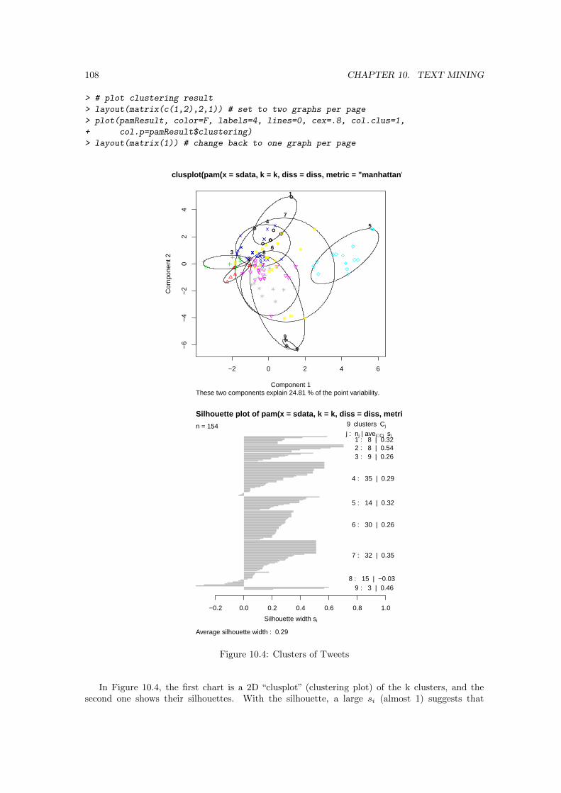
Figure 10.4: Clusters of Tweets

In Figure 10.4, the first chart is a 2D “clusplot” (clustering plot) of the k clusters, and thesecond one shows their silhouettes. With the silhouette, a large si (almost 1) suggests that

10.9. PACKAGES, FURTHER READINGS AND DISCUSSIONS 109

the corresponding observations are very well clustered, a small si (around 0) means that theobservation lies between two clusters, and observations with a negative si are probably placed inthe wrong cluster. The average silhouette width is 0.29, which suggests that the clusters are notwell separated from one another.

The above results and Figure 10.4 show that there are nine clusters of tweets. Clusters 1, 2,3, 5 and 9 are well separated groups, with each of them focusing on a specific topic. Cluster 7is composed of tweets not fitted well into other clusters, and it overlaps all other clusters. Thereis also a big overlap between cluster 6 and 8, which is understandable from their medoids. Someobservations in cluster 8 are of negative silhouette width, which means that they may fit better inother clusters than cluster 8.

To improve the clustering quality, we have also tried to set the range of cluster numberskrange=2:8 when calling pamk(), and in the new clustering result, there are eight clusters, withthe observations in the above cluster 8 assigned to other clusters, mostly to cluster 6. The resultsare not shown in this book, and readers can try it with the code below.

> pamResult2 <- pamk(m3, krange=2:8, metric="manhattan")

10.9 Packages, Further Readings and Discussions

In addition to frequent terms, associations and clustering demonstrated in this chapter, someother possible analysis on the above Twitter text is graph mining and social network analysis. Forexample, a graph of words can be derived from a document-term matrix, and then we can usetechniques for graph mining to find links between words and groups of words. A graph of tweets(documents) can also be generated and analyzed in a similar way. It can also be presented andanalyzed as a bipartite graph with two disjoint sets of vertices, that is, words and tweets. We willdemonstrate social network analysis on the Twitter data in Chapter 11: Social Network Analysis.

Some R packages for text mining are listed below.

� Package tm [Feinerer, 2012]: A framework for text mining applications within R.

� Package tm.plugin.mail [Feinerer, 2010]: Text Mining E-Mail Plug-In. A plug-in for the tmtext mining framework providing mail handling functionality.

� package textcat [Hornik et al., 2012] provides n-Gram Based Text Categorization.

� lda [Chang, 2011] fit topic models with LDA (latent Dirichlet allocation)

� topicmodels [Grun and Hornik, 2011] fit topic models with LDA and CTM (correlated topicsmodel)

For more information and examples on text mining with R, some online resources are:

� Introduction to the tm Package – Text Mining in Rhttp://cran.r-project.org/web/packages/tm/vignettes/tm.pdf

� Text Mining Infrastructure in R [Feinerer et al., 2008]http://www.jstatsoft.org/v25/i05

� Text Mining Handbookhttp://www.casact.org/pubs/forum/10spforum/Francis_Flynn.pdf

� Distributed Text Mining in Rhttp://epub.wu.ac.at/3034/

� Text mining with Twitter and Rhttp://heuristically.wordpress.com/2011/04/08/text-data-mining-twitter-r/