Embed Size (px)
Citation preview
RANDOMIZED EXPERIMENTS (CHAPTER 2)
BIOS 776 1 §2 Randomized Experiments
Randomized Experiments (§2)
• Outline
§2.1 Randomization
§2.2 Conditional randomization
§2.3 Standardization
§2.4 Inverse probability weighting
BIOS 776 2 §2 Randomized Experiments
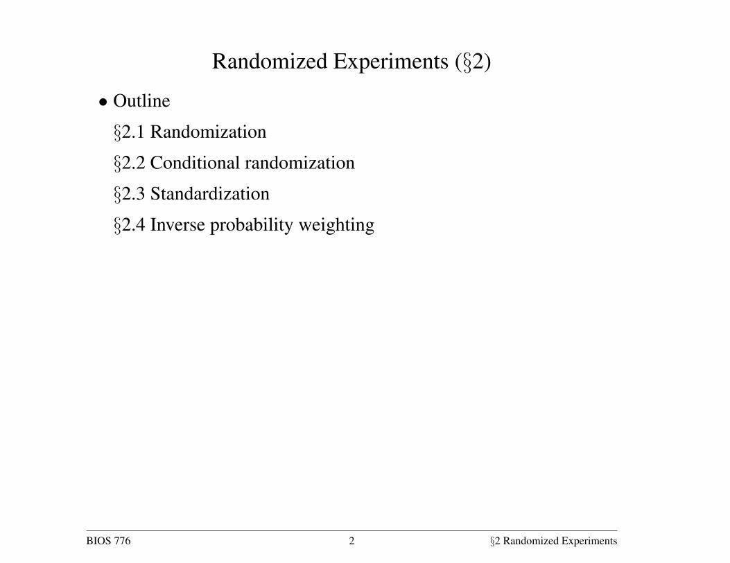
Motivating Example (§2.1)14 Causal Inference
assigned the subject to the white group if the coin turned tails, and to the grey
group if it turned heads. Note this was not a fair coin because the probabilityTable 2.1 0 1
Rheia 0 0 0 ?
Kronos 0 1 1 ?
Demeter 0 0 0 ?
Hades 0 0 0 ?
Hestia 1 0 ? 0
Poseidon 1 0 ? 0
Hera 1 0 ? 0
Zeus 1 1 ? 1
Artemis 0 1 1 ?
Apollo 0 1 1 ?
Leto 0 0 0 ?
Ares 1 1 ? 1
Athena 1 1 ? 1
Hephaestus 1 1 ? 1
Aphrodite 1 1 ? 1
Cyclope 1 1 ? 1
Persephone 1 1 ? 1
Hermes 1 0 ? 0
Hebe 1 0 ? 0
Dionysus 1 0 ? 0
of heads was less than 50%–fewer people ended up in the grey group than
in the white group. Next we asked our research assistants to administer the
treatment of interest ( = 1), to subjects in the white group and a placebo
( = 0) to those in the grey group. Five days later, at the end of the study,
we computed the mortality risks in each group, Pr[ = 1| = 1] = 03 and
Pr[ = 1| = 0] = 06. The associational risk ratio was 0306 = 05 and theassociational risk difference was 03 − 06 = −03. We will assume that thiswas an ideal randomized experiment in all other respects: no loss to follow-
up, full adherence to the assigned treatment over the duration of the study,
a single version of treatment, and double blind assignment (see Chapter 9).
Ideal randomized experiments are unrealistic but useful to introduce some key
concepts for causal inference. Later in this book we consider more realistic
randomized experiments.
Now imagine what would have happened if the research assistants had
misinterpreted our instructions and had treated the grey group rather than
the white group. Say we learned of the misunderstanding after the study
finished. How does this reversal of treatment status affect our conclusions?
Not at all. We would still find that the risk in the treated (now the grey group)
Pr[ = 1| = 1] is 03 and the risk in the untreated (now the white group)
Pr[ = 1| = 0] is 06. The association measure would not change. Becausesubjects were randomly assigned to white and grey groups, the proportion
of deaths among the exposed, Pr[ = 1| = 1] is expected to be the same
whether subjects in the white group received the treatment and subjects in
the grey group received placebo, or vice versa. When group membership is
randomized, which particular group received the treatment is irrelevant for
the value of Pr[ = 1| = 1]. The same reasoning applies to Pr[ = 1| = 0],of course. Formally, we say that groups are exchangeable.
Exchangeability means that the risk of death in the white group would have
been the same as the risk of death in the grey group had subjects in the white
group received the treatment given to those in the grey group. That is, the risk
under the potential treatment value among the treated, Pr[ = 1| = 1],
equals the risk under the potential treatment value among the untreated,
Pr[ = 1| = 0], for both = 0 and = 1. An obvious consequence of these
(conditional) risks being equal in all subsets defined by treatment status in the
population is that they must be equal to the (marginal) risk under treatment
value in the whole population: Pr[ = 1| = 1] = Pr[ = 1| = 0] =
Pr[ = 1]. Because the counterfactual risk under treatment value is the
same in both groups = 1 and = 0, we say that the actual treatment
does not predict the counterfactual outcome . Equivalently, exchangeability
means that the counterfactual outcome and the actual treatment are indepen-
dent, or `
, for all values . Randomization is so highly valued because itExchangeability:
`
for all is expected to produce exchangeability. When the treated and the untreated
are exchangeable, we sometimes say that treatment is exogenous, and thus
exogeneity is commonly used as a synonym for exchangeability.
The previous paragraph argues that, in the presence of exchangeability, the
counterfactual risk under treatment in the white part of the population would
equal the counterfactual risk under treatment in the entire population. But the
risk under treatment in the white group is not counterfactual at all because the
white group was actually treated! Therefore our ideal randomized experiment
allows us to compute the counterfactual risk under treatment in the population
Pr[ =1 = 1] because it is equal to the risk in the treated Pr[ = 1| = 1] =
BIOS 776 3 §2 Randomized Experiments
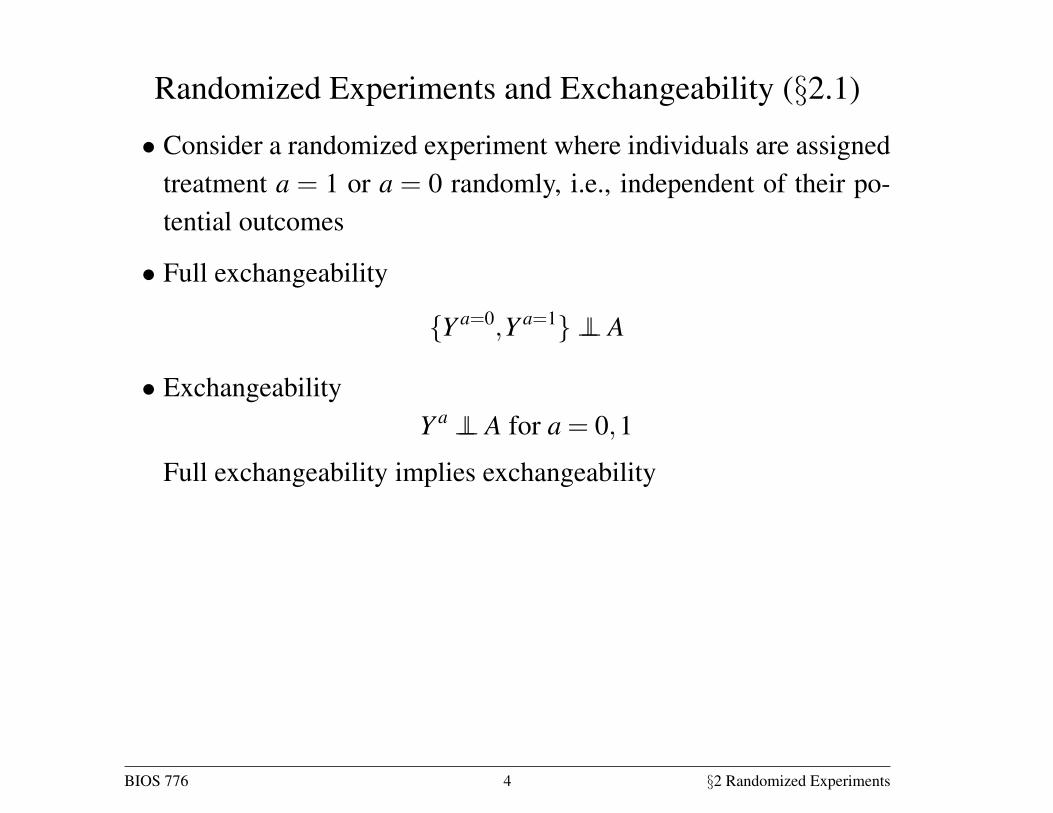
Randomized Experiments and Exchangeability (§2.1)
• Consider a randomized experiment where individuals are assignedtreatment a = 1 or a = 0 randomly, i.e., independent of their po-tential outcomes
• Full exchangeability
{Y a=0,Y a=1} ⊥⊥ A
• ExchangeabilityY a ⊥⊥ A for a = 0,1
Full exchangeability implies exchangeability
BIOS 776 4 §2 Randomized Experiments
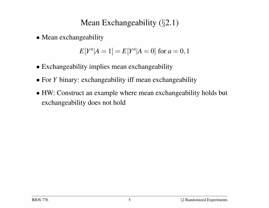
Mean Exchangeability (§2.1)
• Mean exchangeability
E[Y a|A = 1] = E[Y a|A = 0] for a = 0,1
• Exchangeability implies mean exchangeability
• For Y binary: exchangeability iff mean exchangeability
• HW: Construct an example where mean exchangeability holds butexchangeability does not hold
BIOS 776 5 §2 Randomized Experiments
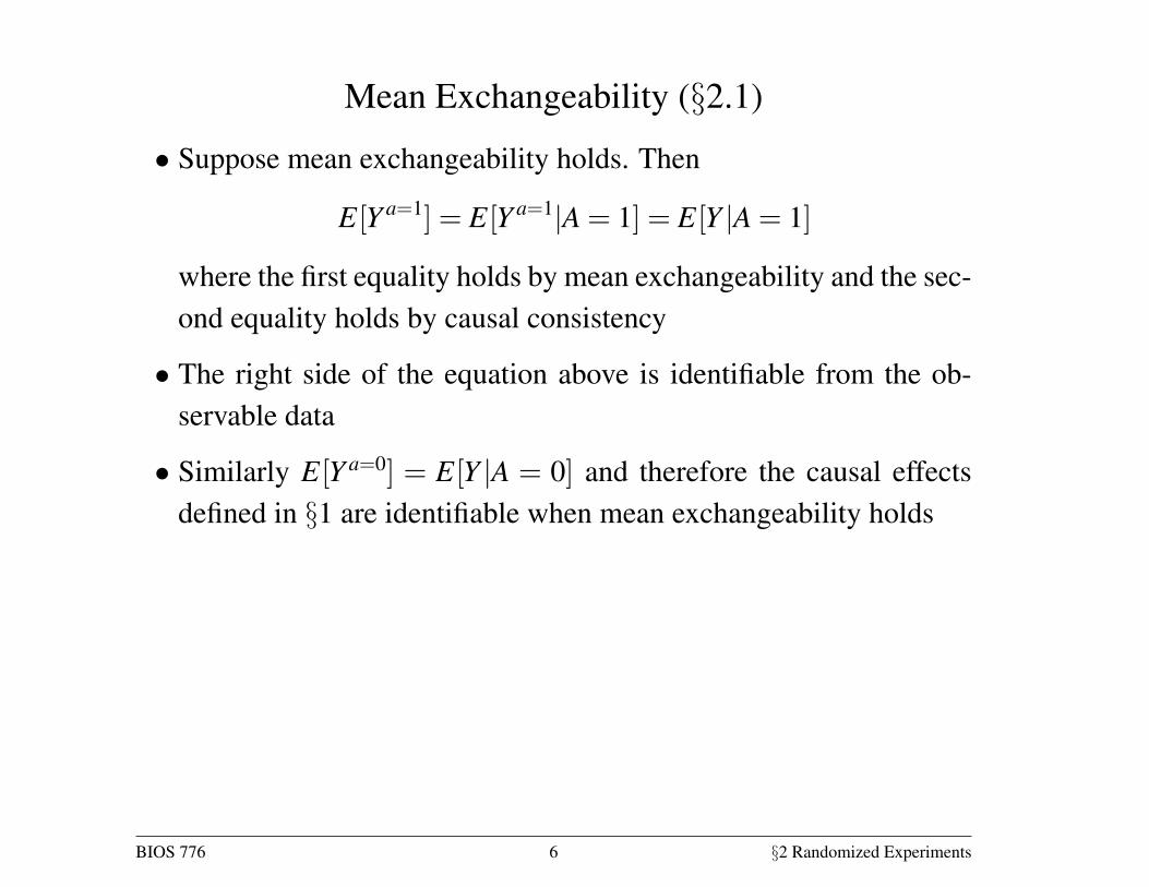
Mean Exchangeability (§2.1)
• Suppose mean exchangeability holds. Then
E[Y a=1] = E[Y a=1|A = 1] = E[Y |A = 1]
where the first equality holds by mean exchangeability and the sec-ond equality holds by causal consistency
• The right side of the equation above is identifiable from the ob-servable data
• Similarly E[Y a=0] = E[Y |A = 0] and therefore the causal effectsdefined in §1 are identifiable when mean exchangeability holds
BIOS 776 6 §2 Randomized Experiments
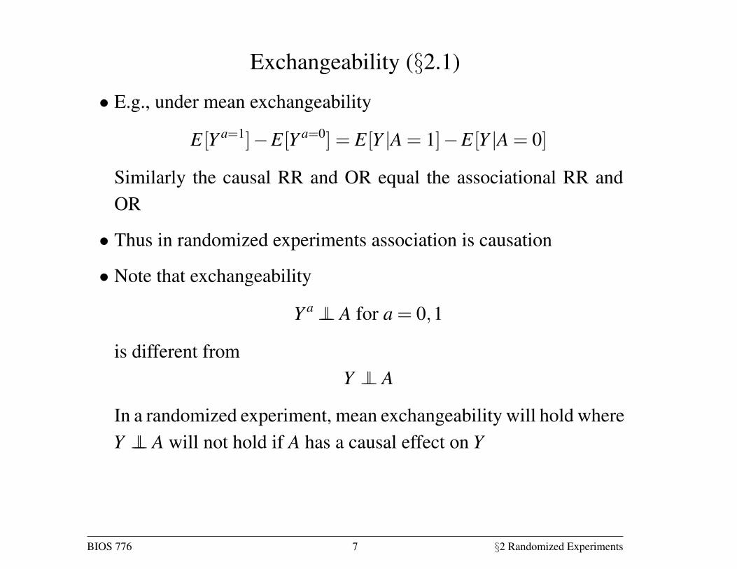
Exchangeability (§2.1)
• E.g., under mean exchangeability
E[Y a=1]−E[Y a=0] = E[Y |A = 1]−E[Y |A = 0]
Similarly the causal RR and OR equal the associational RR andOR
• Thus in randomized experiments association is causation
• Note that exchangeability
Y a ⊥⊥ A for a = 0,1
is different fromY ⊥⊥ A
In a randomized experiment, mean exchangeability will hold whereY ⊥⊥ A will not hold if A has a causal effect on Y
BIOS 776 7 §2 Randomized Experiments
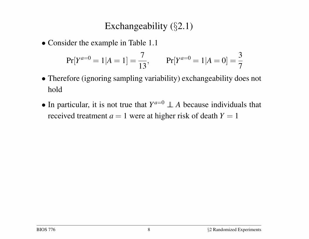
Exchangeability (§2.1)
• Consider the example in Table 1.1
Pr[Y a=0 = 1|A = 1] =7
13, Pr[Y a=0 = 1|A = 0] =
37
• Therefore (ignoring sampling variability) exchangeability does nothold
• In particular, it is not true that Y a=0 ⊥⊥ A because individuals thatreceived treatment a = 1 were at higher risk of death Y = 1
BIOS 776 8 §2 Randomized Experiments
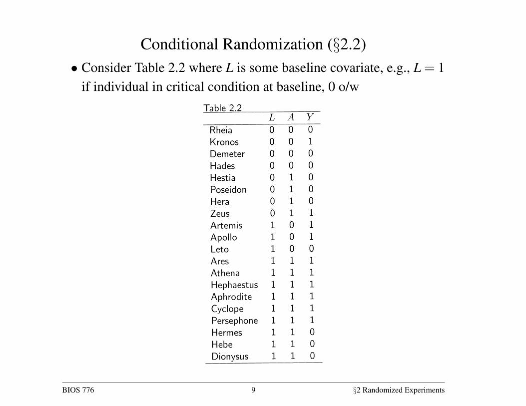
Conditional Randomization (§2.2)• Consider Table 2.2 where L is some baseline covariate, e.g., L = 1
if individual in critical condition at baseline, 0 o/w
Randomized experiments 17
outcome (1 if the subject died, 0 otherwise), Table 2.2 also contains data on
the prognosis factor (1 if the subject was in critical condition, 0 otherwise),
which we measured before treatment was assigned. We now consider two mu-
tually exclusive study designs and discuss whether the data in Table 2.2 could
have arisen from either of them.
In design 1 we would have randomly selected 65% of the individuals in the
population and transplanted a new heart to each of the selected individuals.
That would explain why 13 out of 20 subjects were treated. In design 2 weTable 2.2
Rheia 0 0 0
Kronos 0 0 1
Demeter 0 0 0
Hades 0 0 0
Hestia 0 1 0
Poseidon 0 1 0
Hera 0 1 0
Zeus 0 1 1
Artemis 1 0 1
Apollo 1 0 1
Leto 1 0 0
Ares 1 1 1
Athena 1 1 1
Hephaestus 1 1 1
Aphrodite 1 1 1
Cyclope 1 1 1
Persephone 1 1 1
Hermes 1 1 0
Hebe 1 1 0
Dionysus 1 1 0
would have classified all individuals as being in either critical ( = 1) or
noncritical ( = 0) condition. Then we would have randomly selected 75% of
the individuals in critical condition and 50% of those in noncritical condition,
and transplanted a new heart to each of the selected individuals. That would
explain why 9 out of 12 subjects in critical condition, and 4 out of 8 subjects
in non critical condition, were treated.
Both designs are randomized experiments. Design 1 is precisely the type
of randomized experiment described in Section 2.1. Under this design, we
would use a single coin to assign treatment to all subjects (e.g., treated if tails,
untreated if heads): a loaded coin with probability 065 of turning tails, thus
resulting in 65% of the subjects receiving treatment. Under design 2 we would
not use a single coin for all subjects. Rather, we would use a coin with a 075
chance of turning tails for subjects in critical condition, and another coin with
a 050 chance of turning tails for subjects in non critical condition. We refer to
design 2 experiments as conditionally randomized experiments because we use
several randomization probabilities that depend (are conditional) on the values
of the variable . We refer to design 1 experiments as marginally randomized
experiments because we use a single unconditional (marginal) randomization
probability that is common to all subjects.
As discussed in the previous section, a marginally randomized experiment
is expected to result in exchangeability of the treated and the untreated:
Pr[ = 1| = 1] = Pr[ = 1| = 0] or `
. In contrast, a con-
ditionally randomized experiment will not generally result in exchangeability
of the treated and the untreated because, by design, each group may have a
different proportion of subjects with bad prognosis.
Thus the data in Table 2.2 could not have arisen from a marginally random-
ized experiment because 69% treated versus 43% untreated individuals were
in critical condition. This imbalance indicates that the risk of death in the
treated, had they remained untreated, would have been higher than the risk of
death in the untreated. In other words, treatment predicts the counterfactual
risk of death under no treatment, and exchangeability `
does not hold.
Since our study was a randomized experiment, you can now safely conclude
that the study was a randomized experiment with randomization conditional
on .
Our conditionally randomized experiment is simply the combination of two
separate marginally randomized experiments: one conducted in the subset of
individuals in critical condition ( = 1), the other in the subset of individuals
in non critical condition ( = 0). Consider first the randomized experiment
being conducted in the subset of individuals in critical condition. In this subset,
the treated and the untreated are exchangeable. Formally, the counterfactual
mortality risk under each treatment value is the same among the treated
and the untreated given that they all were in critical condition at the time of
treatment assignment. That is, Pr[ = 1| = 1 = 1] = Pr[ = 1| =
0 = 1] or and are independent given = 1, which is written as
`
| = 1 for all . Similarly, randomization also ensures that the treated
BIOS 776 9 §2 Randomized Experiments
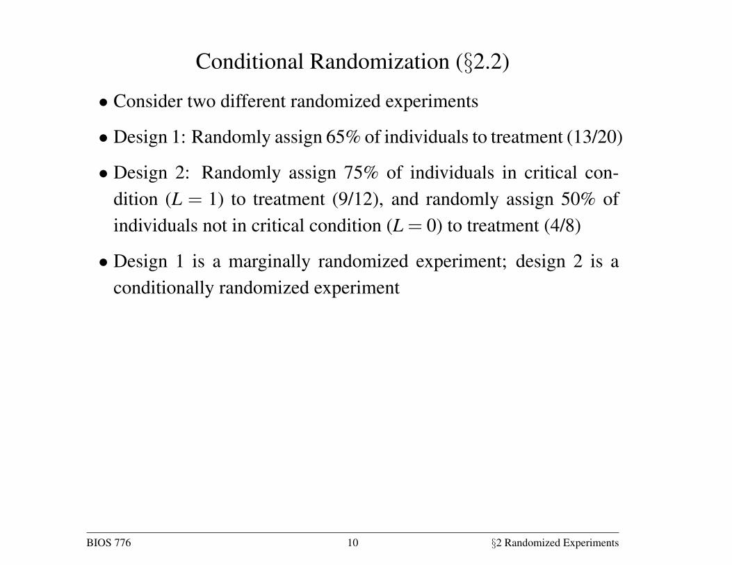
Conditional Randomization (§2.2)
• Consider two different randomized experiments
• Design 1: Randomly assign 65% of individuals to treatment (13/20)
• Design 2: Randomly assign 75% of individuals in critical con-dition (L = 1) to treatment (9/12), and randomly assign 50% ofindividuals not in critical condition (L = 0) to treatment (4/8)
• Design 1 is a marginally randomized experiment; design 2 is aconditionally randomized experiment
BIOS 776 10 §2 Randomized Experiments
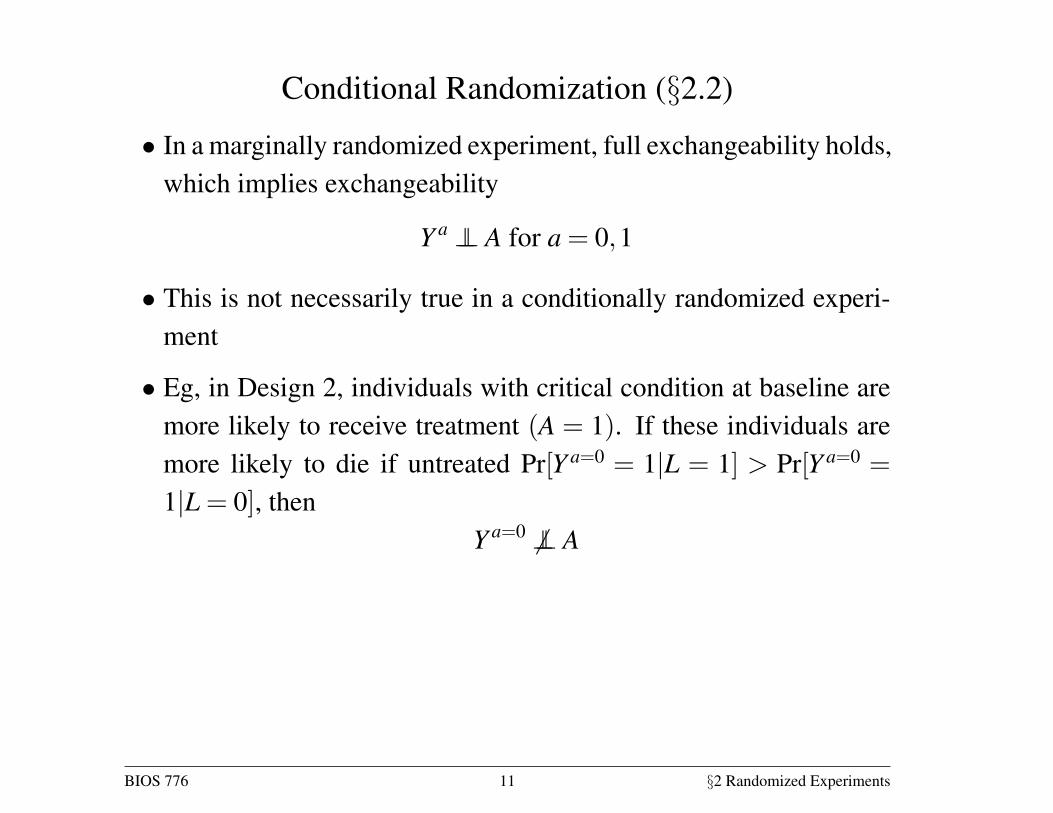
Conditional Randomization (§2.2)
• In a marginally randomized experiment, full exchangeability holds,which implies exchangeability
Y a ⊥⊥ A for a = 0,1
• This is not necessarily true in a conditionally randomized experi-ment
• Eg, in Design 2, individuals with critical condition at baseline aremore likely to receive treatment (A = 1). If these individuals aremore likely to die if untreated Pr[Y a=0 = 1|L = 1] > Pr[Y a=0 =
1|L = 0], thenY a=0 6⊥⊥ A
BIOS 776 11 §2 Randomized Experiments
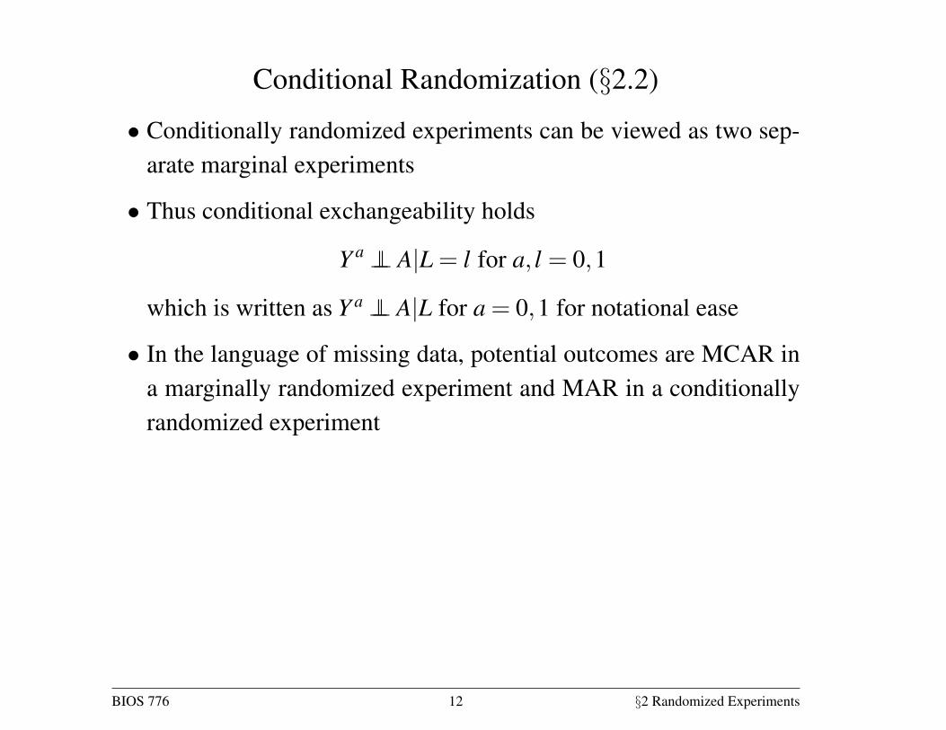
Conditional Randomization (§2.2)
• Conditionally randomized experiments can be viewed as two sep-arate marginal experiments
• Thus conditional exchangeability holds
Y a ⊥⊥ A|L = l for a, l = 0,1
which is written as Y a ⊥⊥ A|L for a = 0,1 for notational ease
• In the language of missing data, potential outcomes are MCAR ina marginally randomized experiment and MAR in a conditionallyrandomized experiment
BIOS 776 12 §2 Randomized Experiments
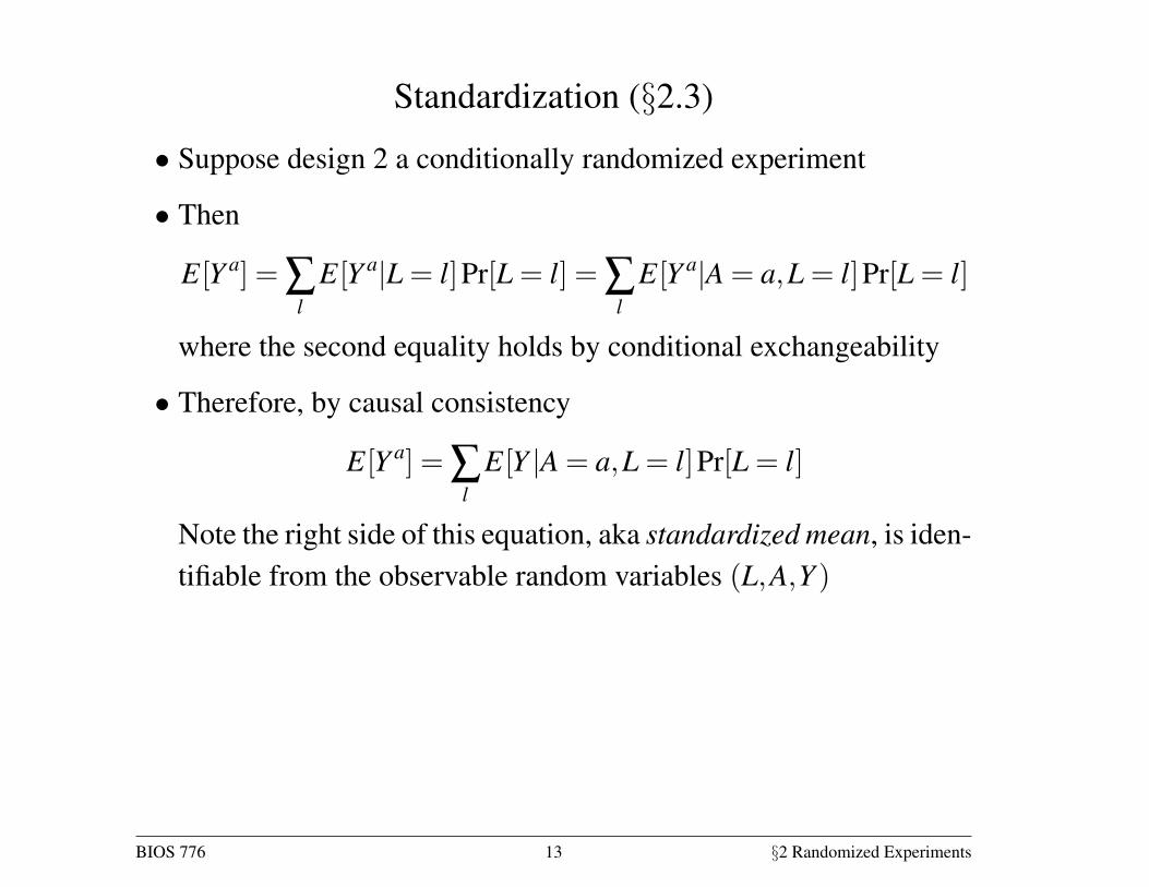
Standardization (§2.3)
• Suppose design 2 a conditionally randomized experiment
• Then
E[Y a] = ∑l
E[Y a|L = l]Pr[L = l] = ∑l
E[Y a|A = a,L = l]Pr[L = l]
where the second equality holds by conditional exchangeability
• Therefore, by causal consistency
E[Y a] = ∑l
E[Y |A = a,L = l]Pr[L = l]
Note the right side of this equation, aka standardized mean, is iden-tifiable from the observable random variables (L,A,Y )
BIOS 776 13 §2 Randomized Experiments
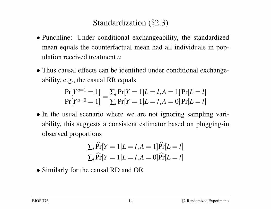
Standardization (§2.3)
• Punchline: Under conditional exchangeability, the standardizedmean equals the counterfactual mean had all individuals in pop-ulation received treatment a
• Thus causal effects can be identified under conditional exchange-ability, e.g., the casual RR equals
Pr[Y a=1 = 1]Pr[Y a=0 = 1]
=∑l Pr[Y = 1|L = l,A = 1]Pr[L = l]∑l Pr[Y = 1|L = l,A = 0]Pr[L = l]
• In the usual scenario where we are not ignoring sampling vari-ability, this suggests a consistent estimator based on plugging-inobserved proportions
∑l P̂r[Y = 1|L = l,A = 1]P̂r[L = l]
∑l P̂r[Y = 1|L = l,A = 0]P̂r[L = l]
• Similarly for the causal RD and OR
BIOS 776 14 §2 Randomized Experiments
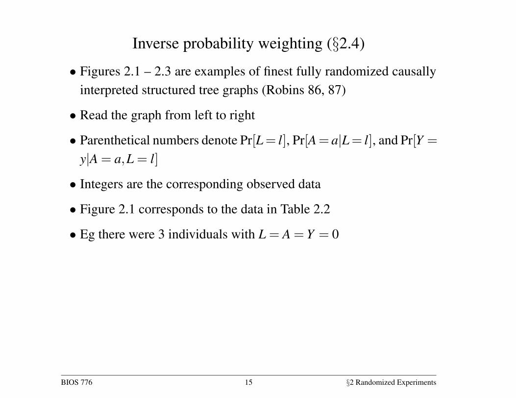
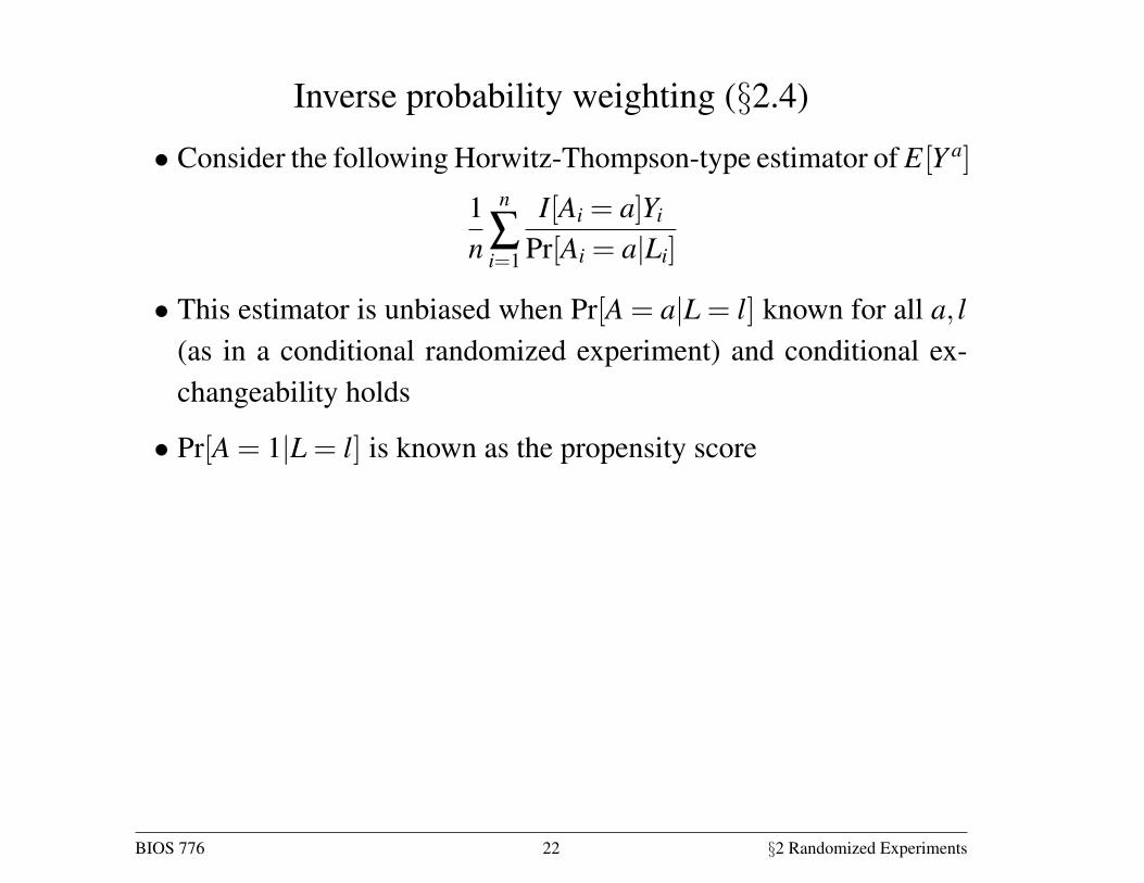
Inverse probability weighting (§2.4)
• Figures 2.1 – 2.3 are examples of finest fully randomized causallyinterpreted structured tree graphs (Robins 86, 87)
• Read the graph from left to right
• Parenthetical numbers denote Pr[L= l], Pr[A= a|L= l], and Pr[Y =
y|A = a,L = l]
• Integers are the corresponding observed data
• Figure 2.1 corresponds to the data in Table 2.2
• Eg there were 3 individuals with L = A = Y = 0
BIOS 776 15 §2 Randomized Experiments
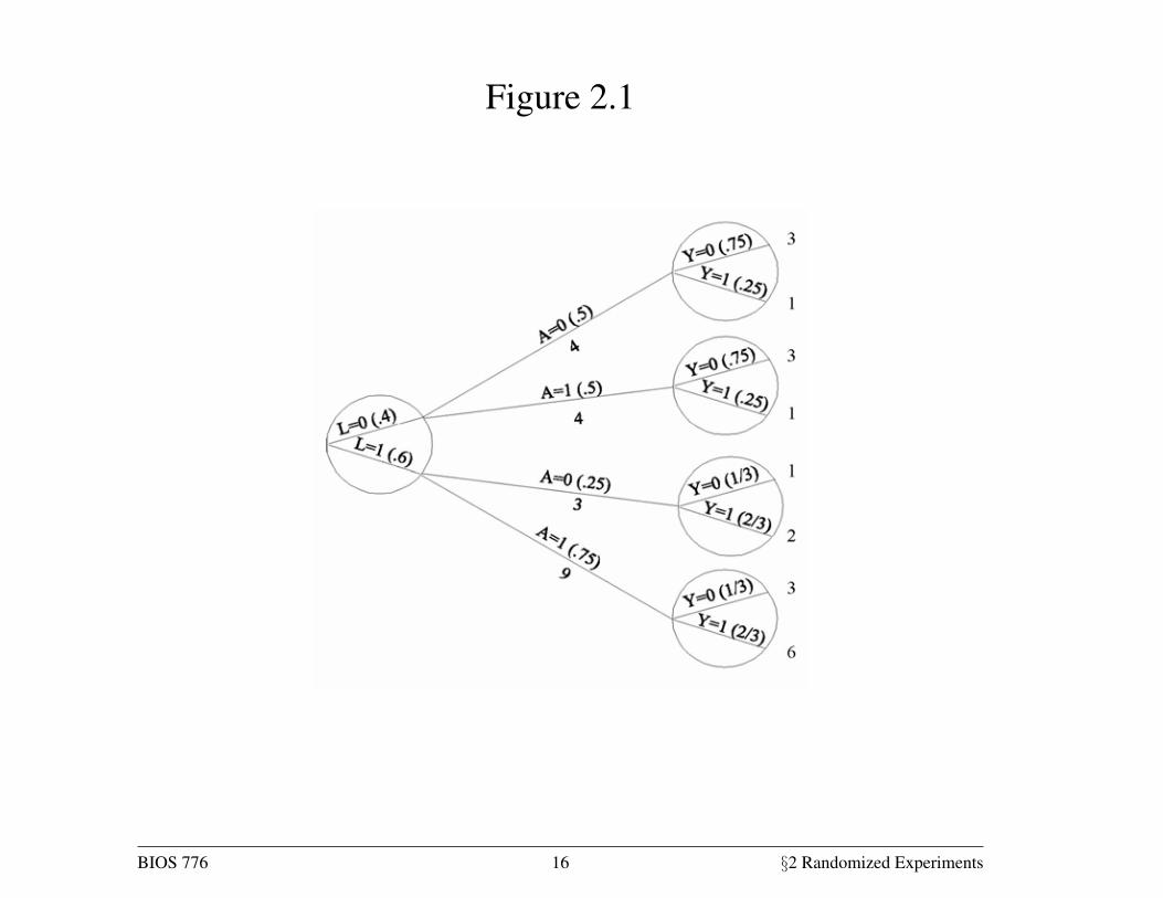
Figure 2.1
20 Causal Inference
2.4 Inverse probability weighting
In the previous section we computed the causal risk ratio in a conditionally
randomized experiment via standardization. In this section we compute this
causal risk ratio via inverse probability weighting. The data in Table 2.2
can be displayed as a tree in which all 20 individuals start at the left and
progress over time towards the right, as in Figure 2.1. The leftmost circle of
the tree contains its first branching: 8 individuals were in non critical condi-
tion ( = 0) and 12 in critical condition ( = 1). The numbers in parenthesesFigure 2.1 is an example of a
finest fully randomized causally in-
terpreted structured tree graph or
FFRCISTG (Robins 1986, 1987).
Did we win the prize for the worst
acronym ever?
are the probabilities of being in noncritical, Pr [ = 0] = 820 = 04, or crit-
ical, Pr [ = 1] = 1220 = 06, condition. Let us follow, for example, the
branch = 0. Of the 8 individuals in this branch, 4 were untreated ( = 0)
and 4 were treated ( = 1). The conditional probability of being untreated
is Pr [ = 0| = 0] = 48 = 05, as shown in parentheses. The conditional
probability of being treated Pr [ = 1| = 0] is 05 too. The upper right circlerepresents that, of the 4 individuals in the branch ( = 0 = 0), 3 survived
( = 0) and 1 died ( = 1). That is, Pr [ = 0| = 0 = 0] = 34 and
Pr [ = 1| = 0 = 0] = 14 The other branches of the tree are interpretedanalogously. The circles contain the bifurcations defined by non treatment
variables. We now use this tree to compute the causal risk ratio.
Figure 2.1
The denominator of the causal risk ratio, Pr[ =0 = 1], is the counterfac-
tual risk of death had everybody in the population remained untreated. Let
us calculate this risk. In Figure 2.1, 4 out of 8 individuals with = 0 were
untreated, and 1 of them died. How many deaths would have occurred had
the 8 individuals with = 0 remained untreated? Two deaths, because if 8
individuals rather than 4 individuals had remained untreated, then 2 deaths
rather than 1 death would have been observed. If the number of individuals is
multiplied times 2, then the number of deaths is also doubled. In Figure 2.1,
3 out of 12 individuals with = 1 were untreated, and 2 of them died. How
many deaths would have occurred had the 12 individuals with = 1 remained
BIOS 776 16 §2 Randomized Experiments
Figures 2.1
• Q: For the 8 individuals with L = 0, how many deaths would weexpect (ignoring sampling variability) had, counter to fact, none ofthem received treatment?
• A:
• Why? What key assumption are we relying on?
BIOS 776 17 §2 Randomized Experiments
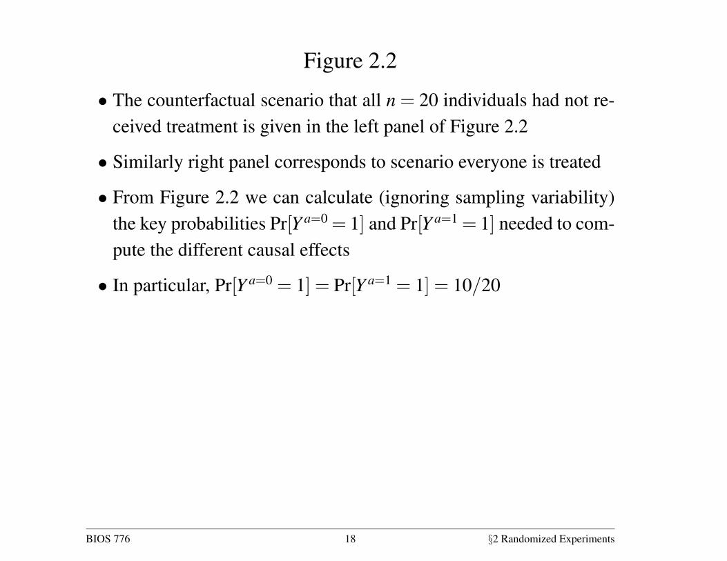
Figure 2.2
• The counterfactual scenario that all n = 20 individuals had not re-ceived treatment is given in the left panel of Figure 2.2
• Similarly right panel corresponds to scenario everyone is treated
• From Figure 2.2 we can calculate (ignoring sampling variability)the key probabilities Pr[Y a=0 = 1] and Pr[Y a=1 = 1] needed to com-pute the different causal effects
• In particular, Pr[Y a=0 = 1] = Pr[Y a=1 = 1] = 10/20
BIOS 776 18 §2 Randomized Experiments
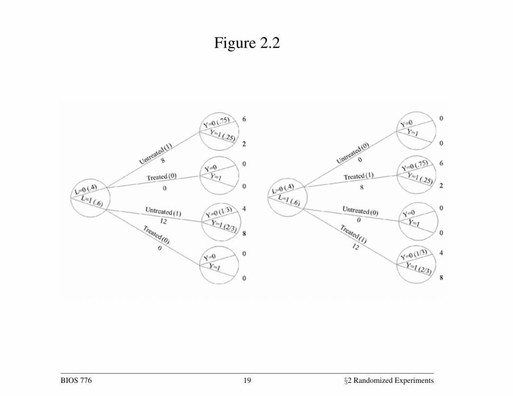
Figure 2.2
Randomized experiments 21
Fine Point 2.2
Risk periods. We have defined a risk as the proportion of subjects who develop the outcome of interest during a
particular period. For example, the 5-day mortality risk in the treated Pr[ = 1| = 0] is the proportion of treated
subjects who died during the first five days of follow-up. Throughout the book we often specify the period when the
risk is first defined (e.g., 5 days) and, for conciseness, omit it later. That is, we may just say “the mortality risk” rather
than “the five-day mortality risk.”
The following example highlights the importance of specifying the risk period. Suppose a randomized experiment
was conducted to quantify the causal effect of antibiotic therapy on mortality among elderly humans infected with the
plague bacteria. An investigator analyzes the data and concludes that the causal risk ratio is 005, i.e., on average
antibiotics decrease mortality by 95%. A second investigator also analyzes the data but concludes that the causal risk
ratio is 1, i.e., antibiotics have a null average causal effect on mortality. Both investigators are correct. The first
investigator computed the ratio of 1-year risks, whereas the second investigator computed the ratio of 100-year risks.
The 100-year risk was of course 1 regardless of whether subjects received the treatment. When we say that a treatment
has a causal effect on mortality, we mean that death is delayed, not prevented, by the treatment.
untreated? Eight deaths, or 2 deaths times 4, because 12 is 3×4. That is, if all8+ 12 = 20 individuals in the population had been untreated, then 2+ 8 = 10
would have died. The denominator of the causal risk ratio, Pr[ =0 = 1], is
1020 = 05. The first tree in Figure 2.2 shows the population had everybody
remained untreated. Of course, these calculations rely on the condition that
treated individuals with = 0, had they remained untreated, would have had
the same probability of death as those who actually remained untreated. This
condition is precisely exchangeability given = 0.
Figure 2.2
The numerator of the causal risk ratio Pr[ =1 = 1] is the counterfactual
risk of death had everybody in the population been treated. Reasoning as in
the previous paragraph, this risk is calculated to be also 1020 = 05, under
exchangeability given = 1. The second tree in Figure 2.2 shows the popu-
lation had everybody been treated. Combining the results from this and the
previous paragraph, the causal risk ratio Pr[ =1 = 1]Pr[ =0 = 1] is equal
to 0505 = 1. We are done.
Let us examine how this method works. The two trees in Figure 2.2 are
essentially a simulation of what would have happened had all subjects in the
BIOS 776 19 §2 Randomized Experiments
Figures 2.2 – 2.3
• Suppose the two counterfactual scenarios in Figure 2.2 are com-bined into a single pseudo-population
• This is depicted in Figure 2.3
• Under conditional exchangeability in the original population Y a ⊥⊥A|L, in the pseudo population we have (unconditional) exchange-ability; association is causation
• The pseudo-population can be viewed as arising from weightingeach individual by the inverse of the conditional probability of re-ceiving the treatment level that she indeed received
BIOS 776 20 §2 Randomized Experiments
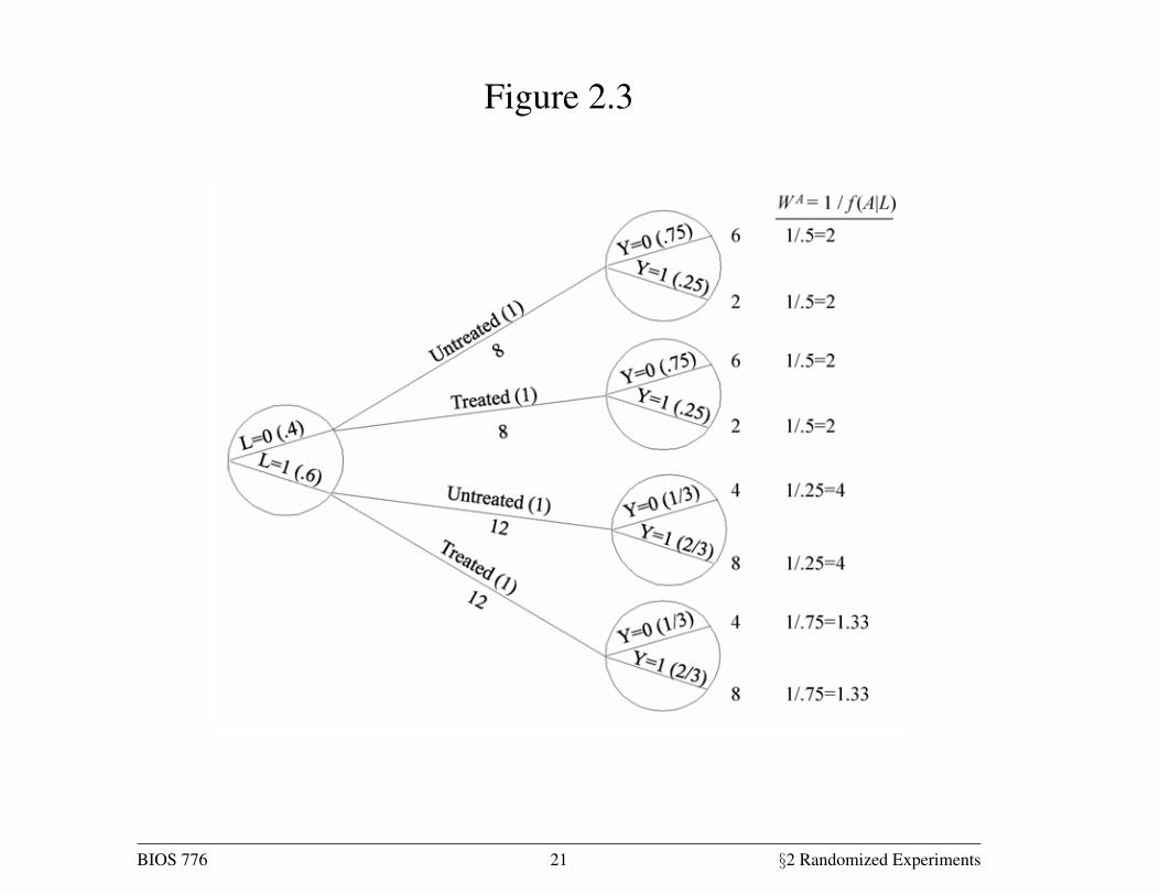
Figure 2.3
22 Causal Inference
population been untreated and treated, respectively. These simulations are
correct under conditional exchangeability. Both simulations can be pooled to
create a hypothetical population in which every individual appears both as a
treated and as an untreated individual. This hypothetical population, twice
as large as the original population, is known as the pseudo-population. Fig-
ure 2.3 shows the entire pseudo-population. Under conditional exchangeability
`
| in the original population, the treated and the untreated are (uncon-ditionally) exchangeable in the pseudo-population because the is independent
of . In other words, the associational risk ratio in the pseudo-population is
equal to the causal risk ratio in both the pseudo-population and the original
population.
This method is known as inverse probability (IP) weighting. To see why,
let us look at, say, the 4 untreated individuals with = 0 in the population
of Figure 2.1. These individuals are used to create 8 members of the pseudo-IP weighted estimators were pro-
posed by Horvitz and Thompson
(1952) for surveys in which subjects
are sampled with unequal probabil-
ities
population of Figure 2.3. That is, each of them is assigned a weight of 2, which
is equal to 105. Figure 2.1 shows that 05 is the conditional probability of
staying untreated given = 0. Similarly, the 9 treated subjects with = 1 in
Figure 2.1 are used to create 12 members of the pseudo-population. That is,
each of them is assigned a weight of 133 = 1075. Figure 2.1 shows that 075
is the conditional probability of being treated given = 1. Informally, the
pseudo-population is created by weighting each individual in the population
by the inverse of the conditional probability of receiving the treatment levelIP weight: = 1 [|]that she indeed received. These IP weights are shown in the last column of
Figure 2.3.
Figure 2.3
IP weighting yielded the same result as standardization–causal risk ra-
tio equal to 1– in our example above. This is no coincidence: standardiza-
tion and IP weighting are mathematically equivalent (see Technical Point 2.3).
Each method uses a different set of the probabilities shown in Figure 2.1: IP
weighting uses the conditional probability of treatment given the covariate
BIOS 776 21 §2 Randomized Experiments
Inverse probability weighting (§2.4)
• Consider the following Horwitz-Thompson-type estimator of E[Y a]
1n
n
∑i=1
I[Ai = a]Yi
Pr[Ai = a|Li]
• This estimator is unbiased when Pr[A = a|L = l] known for all a, l(as in a conditional randomized experiment) and conditional ex-changeability holds
• Pr[A = 1|L = l] is known as the propensity score
BIOS 776 22 §2 Randomized Experiments
Inverse probability weighting (§2.4)
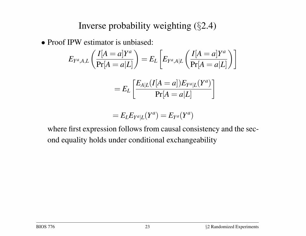
• Proof IPW estimator is unbiased:
EY a,A,L
(I[A = a]Y a
Pr[A = a|L]
)= EL
[EY a,A|L
(I[A = a]Y a
Pr[A = a|L]
)]
= EL
[EA|L(I[A = a])EY a|L(Y a)
Pr[A = a|L]
]
= ELEY a|L(Y a) = EY a(Y a)
where first expression follows from causal consistency and the sec-ond equality holds under conditional exchangeability
BIOS 776 23 §2 Randomized Experiments