Embed Size (px)
Citation preview
R Textbook Companion forMiller and Freund’s Probability and Statistics
for Engineersby Richard A. Johnson1
Created byPrakash Narayan Singh Rautela
B.Sc.Computer Science and Engineering
Vivekanand Education Society’s College of Arts Science & CommerceCross-Checked byR TBC Team
August 28, 2020
1Funded by a grant from the National Mission on Education through ICT- http://spoken-tutorial.org/NMEICT-Intro. This Textbook Companion and Rcodes written in it can be downloaded from the ”Textbook Companion Project”section at the website - https://r.fossee.in.
Book Description
Title: Miller and Freund’s Probability and Statistics for Engineers
Author: Richard A. Johnson
Publisher: Pearson, USA
Edition: 9
Year: 2017
ISBN: 978-0-321-98624-5
1
R numbering policy used in this document and the relation to the abovebook.
Exa Example (Solved example)
Eqn Equation (Particular equation of the above book)
For example, Exa 3.51 means solved example 3.51 of this book. Sec 2.3 meansan R code whose theory is explained in Section 2.3 of the book.
2
Contents
List of R Codes 4
2 Organization and Description of Data 5
3 PROBABILITY 13
4 PROBABILITY DISTRIBUTIONS 24
5 PROBABILITY DENSITIES 36
6 SAMPLING DISTRIBUTIONS 49
7 Inferences Concerning a Mean 52
8 Comparing Two Treatments 60
9 INFERENCES CONCERNING VARIANCES 69
10 INFERENCES CONCERNING PROPORTIONS 73
11 REGRESSION ANALYSIS 81
12 ANALYSIS OF VARIANCE 93
13 Factorial Experimentation 103
14 NONPARAMETRIC TESTS 108
15 The Statistical Content of Quality Improvement Programs 115
3

16 Application to Reliability and Life Testing 117
4
List of R Codes
Exa 2.1 Pareto Diagrams and Dot Diagrams . . . . . . . . . . 5Exa 2.2 Pareto Diagrams and Dot Diagrams . . . . . . . . . . 5Exa 2.3 Frequency Distributions . . . . . . . . . . . . . . . . . 6Exa 2.4 Frequency Distributions . . . . . . . . . . . . . . . . . 6Exa 2.6 Graphs of Frequency Distributions . . . . . . . . . . . 7Exa 2.7 Graphs of Frequency Distributions . . . . . . . . . . . 7Exa 2.8 Descriptive Measures . . . . . . . . . . . . . . . . . . . 8Exa 2.9 Descriptive Measures . . . . . . . . . . . . . . . . . . . 8Exa 2.11 Descriptive Measures . . . . . . . . . . . . . . . . . . . 9Exa 2.12 Descriptive Measures . . . . . . . . . . . . . . . . . . . 9Exa 2.13 Descriptive Measures . . . . . . . . . . . . . . . . . . . 9Exa 2.14 Quartiles and Percentiles . . . . . . . . . . . . . . . . 10Exa 2.15 Quartiles and Percentiles . . . . . . . . . . . . . . . . 11Exa 2.16 Quartiles and Percentiles . . . . . . . . . . . . . . . . 11Exa 2.18 The Calculation of x and s . . . . . . . . . . . . . . . 12Exa 2.19 The Calculation of x and s . . . . . . . . . . . . . . . 12Exa 3.1 Sample Spaces and Events . . . . . . . . . . . . . . . . 13Exa 3.5 Counting . . . . . . . . . . . . . . . . . . . . . . . . . 13Exa 3.6 Counting . . . . . . . . . . . . . . . . . . . . . . . . . 14Exa 3.11 Probability . . . . . . . . . . . . . . . . . . . . . . . . 14Exa 3.13 Probability . . . . . . . . . . . . . . . . . . . . . . . . 14Exa 3.14 The Axioms of Probability . . . . . . . . . . . . . . . 15Exa 3.15 Some Elementary Theorems . . . . . . . . . . . . . . . 16Exa 3.16 Some Elementary Theorems . . . . . . . . . . . . . . . 16Exa 3.17 Some Elementary Theorems . . . . . . . . . . . . . . . 17Exa 3.18 Some Elementary Theorems . . . . . . . . . . . . . . . 17Exa 3.19 Some Elementary Theorems . . . . . . . . . . . . . . . 17Exa 3.20 Conditional Probability . . . . . . . . . . . . . . . . . 18
5
Exa 3.21 Conditional Probability . . . . . . . . . . . . . . . . . 18Exa 3.22 Conditional Probability . . . . . . . . . . . . . . . . . 19Exa 3.24 Conditional Probability . . . . . . . . . . . . . . . . . 19Exa 3.25 Conditional Probability . . . . . . . . . . . . . . . . . 19Exa 3.26 Conditional Probability . . . . . . . . . . . . . . . . . 20Exa 3.28 Conditional Probability . . . . . . . . . . . . . . . . . 20Exa 3.29 Conditional Probability . . . . . . . . . . . . . . . . . 21Exa 3.30 Bayes Theorem . . . . . . . . . . . . . . . . . . . . . . 22Exa 3.31 Bayes Theorem . . . . . . . . . . . . . . . . . . . . . . 22Exa 4.1 Random Variables . . . . . . . . . . . . . . . . . . . . 24Exa 4.3 The Binomial Distribution . . . . . . . . . . . . . . . 25Exa 4.4 The Binomial Distribution . . . . . . . . . . . . . . . 25Exa 4.5 The Binomial Distribution . . . . . . . . . . . . . . . 26Exa 4.6 The Binomial Distribution . . . . . . . . . . . . . . . 26Exa 4.7 The Binomial Distribution . . . . . . . . . . . . . . . 27Exa 4.8 The Hypergeometric Distribution . . . . . . . . . . . . 27Exa 4.9 The Hypergeometric Distribution . . . . . . . . . . . . 27Exa 4.10 The Mean and the Variance of a Probability Distribution 28Exa 4.11 The Mean and the Variance of a Probability Distribution 28Exa 4.12 The Mean and the Variance of a Probability Distribution 29Exa 4.13 The Mean and the Variance of a Probability Distribution 29Exa 4.14 The Mean and the Variance of a Probability Distribution 29Exa 4.15 The Mean and the Variance of a Probability Distribution 30Exa 4.16 The Mean and the Variance of a Probability Distribution 30Exa 4.17 The Mean and the Variance of a Probability Distribution 30Exa 4.18 The Mean and the Variance of a Probability Distribution 31Exa 4.19 Chebyshevs Theorem . . . . . . . . . . . . . . . . . . 31Exa 4.20 Chebyshevs Theorem . . . . . . . . . . . . . . . . . . 31Exa 4.21 The Poisson Distribution and Rare Events . . . . . . . 32Exa 4.22 The Poisson Distribution and Rare Events . . . . . . . 33Exa 4.24 Poisson Processes . . . . . . . . . . . . . . . . . . . . 33Exa 4.25 Poisson Processes . . . . . . . . . . . . . . . . . . . . 34Exa 4.26 The Geometric and Negative Binomial Distribution . . 34Exa 4.27 The Multinomial Distribution . . . . . . . . . . . . . . 35Exa 5.1 Continuous Random Variables . . . . . . . . . . . . . 36Exa 5.2 Continuous Random Variables . . . . . . . . . . . . . 36Exa 5.3 Continuous Random Variables . . . . . . . . . . . . . 36Exa 5.4 Continuous Random Variables . . . . . . . . . . . . . 37
6
Exa 5.5 The Normal Distribution . . . . . . . . . . . . . . . . 37Exa 5.6 The Normal Distribution . . . . . . . . . . . . . . . . 38Exa 5.7 The Normal Distribution . . . . . . . . . . . . . . . . 38Exa 5.8 The Normal Distribution . . . . . . . . . . . . . . . . 39Exa 5.9 The Normal Distribution . . . . . . . . . . . . . . . . 40Exa 5.10 The Normal Distribution . . . . . . . . . . . . . . . . 40Exa 5.11 The Normal Approximation to the Binomial Distribution 40Exa 5.12 The Log Normal Distribution . . . . . . . . . . . . . . 41Exa 5.13 The Log Normal Distribution . . . . . . . . . . . . . . 41Exa 5.14 The Log Normal Distribution . . . . . . . . . . . . . . 42Exa 5.15 The Log Normal Distribution . . . . . . . . . . . . . . 42Exa 5.16 The Gamma Distribution . . . . . . . . . . . . . . . . 43Exa 5.17 The Gamma Distribution . . . . . . . . . . . . . . . . 43Exa 5.18 The Beta Distribution . . . . . . . . . . . . . . . . . . 43Exa 5.19 The Weibull Distribution . . . . . . . . . . . . . . . . 44Exa 5.20 Joint Distributions Discrete and Continuous . . . . . . 44Exa 5.21 Joint Distributions Discrete and Continuous . . . . . . 45Exa 5.22 Joint Distributions Discrete and Continuous . . . . . . 45Exa 5.23 Joint Distributions Discrete and Continuous . . . . . . 46Exa 5.31 Joint Distributions Discrete and Continuous . . . . . . 46Exa 5.42 Checking If the Data Are Normal . . . . . . . . . . . . 47Exa 5.43 Transforming Observations to Near Normality . . . . . 47Exa 5.44 Simulation . . . . . . . . . . . . . . . . . . . . . . . . 47Exa 5.45 Simulation . . . . . . . . . . . . . . . . . . . . . . . . 48Exa 6.49 The Sampling Distribution of the Mean . . . . . . . . 49Exa 6.51 The Sampling Distribution of the Mean . . . . . . . . 49Exa 6.52 The Sampling Distribution of the Mean Sigma Unknown 50Exa 6.53 The Sampling Distribution of the Variance . . . . . . 50Exa 5.54 The Sampling Distribution of the Variance . . . . . . 51Exa 6.55 The Sampling Distribution of the Variance . . . . . . 51Exa 7.2 Point Estimation . . . . . . . . . . . . . . . . . . . . . 52Exa 7.3 Point Estimation . . . . . . . . . . . . . . . . . . . . . 52Exa 7.4 Point Estimation . . . . . . . . . . . . . . . . . . . . . 53Exa 7.5 Point Estimation . . . . . . . . . . . . . . . . . . . . . 53Exa 7.6 Interval Estimation . . . . . . . . . . . . . . . . . . . 53Exa 7.7 Interval Estimation . . . . . . . . . . . . . . . . . . . 54Exa 7.8 Interval Estimation . . . . . . . . . . . . . . . . . . . 54Exa 7.13 Maximum Likelihood Estimation . . . . . . . . . . . . 55
7
Exa 7.15 Maximum Likelihood Estimation . . . . . . . . . . . . 55Exa 7.18 Hypotheses Concerning One Mean . . . . . . . . . . . 56Exa 7.19 Hypotheses Concerning One Mean . . . . . . . . . . . 56Exa 7.20 Hypotheses Concerning One Mean . . . . . . . . . . . 57Exa 7.22 Power Sample Size and Operating Characteristic Curves 57Exa 7.23 Power Sample Size and Operating Characteristic Curves 58Exa 7.24 Power Sample Size and Operating Characteristic Curves 59Exa 8.3 Comparisons Two Independent Large Samples . . . . 60Exa 8.4 Comparisons Two Independent Large Samples . . . . 61Exa 8.5 Comparisons Two Independent Large Samples . . . . 61Exa 8.6 Comparisons Two Independent Large Samples . . . . 62Exa 8.7 Comparisons Two Independent Small Samples . . . . . 63Exa 8.8 Comparisons Two Independent Small Samples . . . . . 63Exa 8.9 Comparisons Two Independent Small Samples . . . . . 64Exa 8.10 Comparisons Two Independent Small Samples . . . . . 65Exa 8.11 Comparisons Two Independent Small Samples . . . . . 66Exa 8.12 Matched Pairs Comparisons . . . . . . . . . . . . . . . 66Exa 8.13 Matched Pairs Comparisons . . . . . . . . . . . . . . . 67Exa 8.14 Matched Pairs Comparisons . . . . . . . . . . . . . . . 67Exa 9.1 The Estimation of Variances . . . . . . . . . . . . . . 69Exa 9.2 The Estimation of Variances . . . . . . . . . . . . . . 69Exa 9.3 Hypotheses Concerning One Variance . . . . . . . . . 70Exa 9.4 Hypotheses Concerning Two Variances . . . . . . . . . 71Exa 9.5 Hypotheses Concerning Two Variances . . . . . . . . . 71Exa 9.6 Hypotheses Concerning Two Variances . . . . . . . . . 72Exa 10.1 Estimation of Proportions . . . . . . . . . . . . . . . . 73Exa 10.2 Estimation of Proportions . . . . . . . . . . . . . . . . 73Exa 10.3 Estimation of Proportions . . . . . . . . . . . . . . . . 74Exa 10.4 Estimation of Proportions . . . . . . . . . . . . . . . . 74Exa 10.5 Estimation of Proportions . . . . . . . . . . . . . . . . 74Exa 10.6 Hypotheses Concerning One Proportion . . . . . . . . 75Exa 10.7 Hypotheses Concerning One Proportion . . . . . . . . 75Exa 10.8 Hypotheses Concerning Several Proportions . . . . . . 76Exa 10.9 Hypotheses Concerning Several Proportions . . . . . . 77Exa 10.10 Hypotheses Concerning Several Proportions . . . . . . 77Exa 10.11 Hypotheses Concerning Several Proportions . . . . . . 78Exa 10.12 Analysis of r x c Tables . . . . . . . . . . . . . . . . . 79Exa 10.13 Analysis of r x c Tables . . . . . . . . . . . . . . . . . 79
8
Exa 10.15 Goodness of Fit . . . . . . . . . . . . . . . . . . . . . 80Exa 11.1 The Method of Least Squares . . . . . . . . . . . . . . 81Exa 11.2 The Method of Least Squares . . . . . . . . . . . . . . 81Exa 11.3 The Method of Least Squares . . . . . . . . . . . . . . 82Exa 11.5 Inferences Based on the Least Squares Estimators . . . 83Exa 11.6 Inferences Based on the Least Squares Estimators . . . 83Exa 11.7 Inferences Based on the Least Squares Estimators . . 84Exa 11.8 Inferences Based on the Least Squares Estimators . . . 85Exa 11.9 Inferences Based on the Least Squares Estimators . . . 86Exa 11.10 Curvilinear Regression . . . . . . . . . . . . . . . . . . 86Exa 11.11 Curvilinear Regression . . . . . . . . . . . . . . . . . . 87Exa 11.12 Multiple Regression . . . . . . . . . . . . . . . . . . . 88Exa 11.14 Correlation . . . . . . . . . . . . . . . . . . . . . . . . 88Exa 11.15 Correlation . . . . . . . . . . . . . . . . . . . . . . . . 89Exa 11.17 Correlation . . . . . . . . . . . . . . . . . . . . . . . . 89Exa 11.18 Correlation . . . . . . . . . . . . . . . . . . . . . . . . 90Exa 11.19 Multiple Linear Regression Matrix Notation . . . . . . 90Exa 11.20 Multiple Linear Regression Matrix Notation . . . . . . 91Exa 11.21 Multiple Linear Regression Matrix Notation . . . . . . 92Exa 12.1 Completely Randomized Designs . . . . . . . . . . . . 93Exa 12.2 Completely Randomized Designs . . . . . . . . . . . . 94Exa 12.3 Completely Randomized Designs . . . . . . . . . . . . 95Exa 12.4 Completely Randomized Designs . . . . . . . . . . . . 96Exa 12.5 Completely Randomized Designs . . . . . . . . . . . . 97Exa 12.6 Randomized Block Designs . . . . . . . . . . . . . . . 98Exa 12.7 Randomized Block Designs . . . . . . . . . . . . . . . 99Exa 12.8 Randomized Block Designs . . . . . . . . . . . . . . . 100Exa 12.9 Multiple Comparisons . . . . . . . . . . . . . . . . . . 101Exa 12.10 Multiple Comparisons . . . . . . . . . . . . . . . . . . 101Exa 12.11 Analysis of Covariance . . . . . . . . . . . . . . . . . . 102Exa 13.1 Two Factor Experiments . . . . . . . . . . . . . . . . 103Exa 13.2 Multifactor Experiments . . . . . . . . . . . . . . . . 104Exa 13.3 Multifactor Experiments . . . . . . . . . . . . . . . . . 105Exa 13.4 Response Surface Analysis . . . . . . . . . . . . . . . . 106Exa 14.1 The Sign Test . . . . . . . . . . . . . . . . . . . . . . 108Exa 14.2 The Sign Test . . . . . . . . . . . . . . . . . . . . . . 108Exa 14.3 Rank Sum Tests . . . . . . . . . . . . . . . . . . . . . 109Exa 14.4 Rank Sum Tests . . . . . . . . . . . . . . . . . . . . . 110
9
Exa 14.5 Correlation Based on Ranks . . . . . . . . . . . . . . . 111Exa 14.6 Tests of Randomness . . . . . . . . . . . . . . . . . . . 111Exa 14.7 Tests of Randomness . . . . . . . . . . . . . . . . . . . 112Exa 14.8 The Kolmogorov Smirnov and Anderson Darling Tests 113Exa 14.9 The Kolmogorov Smirnov and Anderson Darling Tests 114Exa 15.2 Experimental Designs for Quality . . . . . . . . . . . . 115Exa 15.3 Tolerance Limits . . . . . . . . . . . . . . . . . . . . . 115Exa 15.4 Tolerance Limits . . . . . . . . . . . . . . . . . . . . . 116Exa 16.1 Reliability . . . . . . . . . . . . . . . . . . . . . . . . 117Exa 16.2 Reliability . . . . . . . . . . . . . . . . . . . . . . . . 117Exa 16.3 The Exponential Model in Life Testing . . . . . . . . . 118Exa 16.4 The Exponential Model in Life Testing . . . . . . . . . 118
10
Chapter 2
Organization and Descriptionof Data
R code Exa 2.1 Pareto Diagrams and Dot Diagrams
1 #The i n d u s t r i a l e n g i n e e r r e c o r d s the maximum2 #amount o f b a c t e r i a p r e s e n t a l ong the p r oduc t i on
l i n e , i n the u n i t s Aerob i c P l a t e3 #Count per squa r e i n ch (APC/ i n 2 ) , f o r n = 7 day4 Data <-c(96.3 ,155.6 ,3408.0 ,333.3 ,122.2 ,38.9 ,58.0)#7
day data5 stripchart(Data ,method =” s t a c k ”,6 at = c(0.1),las=1,xlab = ” Ba c t e r i a Count
(APC/ sq . i n ) ”,pch =20)
R code Exa 2.2 Pareto Diagrams and Dot Diagrams
1 #Two Produc t i on hea t s o f we ld ing Ma t e r i a l2 heat1 <-c(0.27 ,0.35 ,0.37)
3 heat2 <-c(0.23 ,0.15 ,0.25 ,0.24 ,0.30 ,0.33 ,0.26)
4 data <-list(heat1 ,heat2)
11
5 stripchart(data ,
6 xlab=”Copper Content ”,7 col=c(” orange ”,” red ”),8 pch=16,
9 method =” s t a c k ”,10 cex=1,
11 xlim=c(0.15 ,0.40) ,
12 las=1
13 )
R code Exa 2.3 Frequency Distributions
1 #c l a s s mark and c l a s s i n t e r v a l s2 message(” C l a s s marks a r e : ”)3 message ((205+245)/2,” ” ,(245+285)/2,” , ” ,(285+325)/
2,” , ” ,(325+365)/2,” , ” ,(365+405)/2)4 print(” C l a s s I n t e r v a l i s ”)5 message (405 -365)
R code Exa 2.4 Frequency Distributions
1 #Data o f 50 n a n o p i l l a r s2 Data <-c(245 ,333 ,296 ,304 ,276 ,336 ,289 ,234 ,253 ,292 ,
3 366 ,323 ,309 ,284 ,310 ,338 ,297 ,314 ,305 ,330 ,
4 266 ,391 ,315 ,305 ,290 ,300 ,292 ,311 ,272 ,312 ,
5 315 ,355 ,346 ,337 ,303 ,265 ,278 ,276 ,373 ,271 ,
6 308 ,276 ,364 ,390 ,298 ,290 ,308 ,221 ,274 ,343)
7 breaks = seq(205, 405, by=40)
8 Data.cut = cut(Data , breaks , right=TRUE)
9 Data.freq = table(Data.cut)
10 cumfreq = cumsum(Data.freq)
11 message(”Cumulat ive Frequency o f data ”)12 cbind(cumfreq)
12
R code Exa 2.6 Graphs of Frequency Distributions
1 #Histogram o f i n t e r r e q u e s t t ime data2 data=c
(2808 ,4201 ,3848 ,9112 ,2082 ,5913 ,1620 ,6719 ,21657 ,
3 3072 ,2949 ,11768 ,4731 ,14211 ,1583 ,9853 ,78811 ,6655 ,
4 1803 ,7012 ,1892 ,4227 ,6583 ,15147 ,4740 ,8528 ,10563 ,
5 43003 ,16723 ,2613 ,26463 ,34867 ,4191 ,4030 ,2472 ,28840 ,
6 24487 ,14001 ,15241 ,1643 ,5732 ,5419 ,28608 ,2487 ,995 ,
7 3116 ,29508 ,11440 ,28336 ,3440
8 )
9 #I t has an long−r i g h t data t a i l10 hist(data ,ylab=” C l a s s f r e qu en cy ”, xlab=” t ime ”)
R code Exa 2.7 Graphs of Frequency Distributions
1 #den s i t y h i s t og ram2 #58 spec imens o f new aluminum a l l o y unde rgo ing
deve lopment3 data <-c
(66.4 ,67.7 ,68.0 ,68.0 ,68.3 ,68.4 ,68.6 ,68.8 ,68.9 ,69.0 ,69.1 ,
4 69.2 ,69.3 ,69.3 ,69.5 ,69.5 ,69.6 ,69.7 ,69.8 ,69.8 ,69.9 ,70.0 ,
5 70.0 ,70.1 ,70.2 ,70.3 ,70.3 ,70.4 ,70.5 ,70.6 ,70.6 ,70.8 ,70.9 ,
6 71.0 ,71.1 ,71.2 ,71.3 ,71.3 ,71.5 ,71.6 ,71.6 ,71.7 ,71.8 ,71.8 ,
13
7 71.9 ,72.1 ,72.2 ,72.3 ,72.4 ,72.6 ,72.7 ,72.9 ,73.1 ,73.3 ,73.5 ,
8 72.4 ,74.5 ,75.3
9 )
10 hist(data ,freq=FALSE ,xlab=” T e an s i l e S t r eng th ”)11 lines(density(data))
R code Exa 2.8 Descriptive Measures
1 #Mean and v a r i a n c e2 data <-c(100 ,45 ,60 ,130 ,30)#t h i s i s a u n i v e r s i t y
s t ud en t s r e sponded f o r t ime i n s o c i a l media3 #Using f u n c t i o n4 mean(data)
5 median(data)
6 #Without f u n c t i o n7 xbar=sum(data)/length(data)
8 xbar
9 med=data[ceiling(length(data)/2)]
10 med
11 cat(”mean and median o f data i s ”,xbar , ’ and ’ ,med)
R code Exa 2.9 Descriptive Measures
1 ?stripchart ()
2 data <-c(11,9,17,19,4,15)
3 mean(data)
4 median(data)
5 stripchart(data ,method =” s t a c k ”,6 at = c(0.1),
7 cex=1,pch=20,
8 xlim=c(0 ,20),
9 las=1,
14
10 main=”Data”,xlab = ”Email − Request ”)
R code Exa 2.11 Descriptive Measures
1 #Var iance2 time <-c(0.6 ,1.2 ,0.9 ,1.0 ,0.6 ,.8)
3 xbar=mean(time)
4 xbar#Mean5 diff=time -xbar
6 diffsq=diff**2
7 diffsum=sum(diffsq)
8 n=length(time)
9 var1=diffsum/(n-1)
10 cat(” Var i ance i s ”,var1)11 #us i ng f u n c t i o n12 var(time)
R code Exa 2.12 Descriptive Measures
1 Time = c(0.6, 1.2,0.9, 1 ,0.6 ,0.8)#de l ay Time2 sd=sd(Time)
3 message(” s tandard d e v i a t i o n i s : ”,sd ,” min”)
R code Exa 2.13 Descriptive Measures
1 #Co e f f i c i e n t o f v a r i e n c e2 #a ) f i r s t micrometer o b s e r v a t i o n3 mean =3.92
4 sd =0.015
5 CV=sd/mean*100
15
6 CV
7 #a ) second micrometer o b s e r v a t i o n8 mean2 =1.54
9 sd2 =0.008
10 CV2=sd2/mean2*100
11 CV2
12 if(CV2 >CV)
13 {
14 print(”measurment mead by f i r s t micrometer i s morep r e c i s e ”)
15 }else
16 {
17 print(”measurment mead by second micrometer i smore p r e c i s e ”)
18 }
R code Exa 2.14 Quartiles and Percentiles
1 #qu a n t i l e and p e r c e n t i l e2 data <-c(136 ,143 ,147 ,151 ,158 ,160 ,
3 161 ,163 ,165 ,167 ,173 ,174 ,
4 181 ,181 ,185 ,188 ,190 ,205)
5 options(digits = 1)
6 data2=quantile(data ,c(.25 ,.5 ,.75))
7 Q1=data2 [1]
8 Q2=data2 [2]
9 Q3=data2 [3]
10 percentile=data[ceiling (0.1*18)]
11 cat(” f i r s t q u a r t i l e i s ”,Q1)12 cat(” second q u a r t i l e i s ”,Q2)13 cat(” t h i r d q u a r t i l e i s ”,Q3)14 cat(”10% p e r c e n t i l e i s ”,percentile)
16
R code Exa 2.15 Quartiles and Percentiles
1 #Range and i n t e r q u a r t i l e range2 Data <-c(136 ,143 ,147 ,151 ,158 ,160 ,
3 161 ,163 ,165 ,167 ,173 ,174 ,
4 181 ,181 ,185 ,188 ,190 ,205)
5 min=min(Data)
6 max=max(Data)
7 range=max -min
8 interrange=IQR(Data)
9 message(” range : ”,range ,” Mpa”)10 message(” i n t e r q u a r t i l e range : ”,interrange ,”Mpa”)
R code Exa 2.16 Quartiles and Percentiles
1 time <-c
(.021 ,.107 ,.179 ,.190 ,.196 ,.283 ,.580 ,.854 ,1.18 ,2.00 ,7.30)
2 boxplot(time , horizontal = TRUE ,ylim=c(0,8),xlab= ’Time ( s ) ’ )
3 quantile=quantile(time ,probs = c(0 ,0.25 ,.5 ,.75 ,1))
4 #minimum5 min=quantile [1]
6 min
7 #maimum8 max=quantile [5]
9 max
10 #Q111 Q1 =0.179
12 Q1
13 #Q314 Q3=1.18
15 Q3
16 #i n t e r q u a r t i l e range i s17 inter=Q3-Q1
17
18 inter
R code Exa 2.18 The Calculation of x and s
1 #20 t e s t runs per fo rmed on urban roads with ani n t e rmed i a t e−s i z e c a r .
2 data <-c(19.7 ,21.5 ,22.5 ,22.2 ,22.6
3 ,21.9 ,20.5 ,19.3 ,19.9 ,21.7
4 ,22.8 ,23.2 ,21.4 ,20.8 ,19.4
5 ,22.0 ,23.0 ,21.1 ,20.9 ,21.3)
6 xbar=mean(data)
7 var=var(data)
8 message(”mean : ”,xbar ,” mpg ”,” s tandard d e v i a t i o n ”,var ,” mpg”)
R code Exa 2.19 The Calculation of x and s
1 #Var iance and mean o f group data2 xi=c(225 ,265 ,305 ,345 ,385)
3 options(digits = 2)
4 fi=c(3,11,23,9,4)
5 n=sum(fi)
6 mean=weighted.mean(xi,fi)
7 var=(sum(xi^2*fi)-sum(xi*fi)^2/n)/(n-1)
8 sd=sqrt(var)
9 cat(”mean : ”,mean ,” var : ”,var ,” sd : ”,sd)
18
Chapter 3
PROBABILITY
R code Exa 3.1 Sample Spaces and Events
1 library(sets)#To import the l i b r a r y f o r s e t2 s=set(pair (0,0),pair (0,1),pair (1,0),pair (2,0),pair
(1,1),pair (0,2))#Sample space3 s
4 C=set(pair (1,0),pair (0 ,1.0))
5 C
6 D=set(pair (0,0),pair (0,1),pair (0,2))
7 D
8 E=set(pair (0,0),pair (1,1))
9 E
10 #Union o f the S e t s11 set_union(C,E)
12 #I n t e r s e c t i o n o f the s e t13 cset_intersection(C,D)
14 #Complement o f the s e t15 set_complement(D,s)
R code Exa 3.5 Counting
19
1 #There a r e t o t a l 12 t rue− f a l s e q u e s t i o n i n how manyway the s tuden t can mark the qu e s t i o n paper
2 #Sin c e each qu e s t i o n can answer i n two ways , t h e r ea r e a l t o g e t h e r
3 Possibility =2^12
4 message(”The s tuden t can marks the qu e s t i o n i n : ”,Possibility ,” p o s s i b l e ways”)
R code Exa 3.6 Counting
1 #( a )2 n1=4#Tota l o p e r a t o r3 n2=3#Tota l Machines4 Pair=n1*n2
5 message(” Tota l ope ra to r−machine p a i r s a r e : ”,Pair)6 #(b )7 n3=8#t e s t spec iment8 message(” Tota l t e s t spec iment r e q u i r e d f o r the
e n t i r e p r oduc t i on i s : ”,n3*Pair)
R code Exa 3.11 Probability
1 #Tota l no o f ways to s e l e c t ace from we l l−s h u f f l e ddeck o f ca rd
2 n=52#Tota l no o f c a rd s3 s=4#Tota l ace4 message(” Tota l p r o b a b i l i t y o f drawing an ace from
deck o f ca rd i s : ”,s/n)
R code Exa 3.13 Probability
20
1 n=300#Tota l i n s u l a t o r2 t=294#Tota l i n s u l a t e r w i th s tand the therma l shock3 message(”The P r o b a b i l i t y tha t any un t e s t ed i n s u l a t o r
w i l l be ab l e to w i th s tand the therma l shock i s :”,t/n)
R code Exa 3.14 The Axioms of Probability
1 #P e rm i s s i b i l i t y o f p r o b a b i l i t y2 #i f3 #1)0<=p(A)<=1 f o r each event A in S4 #2)P( S )=15 #3)A and B ar e Mutual ly Ex c l u s i v e i n event6 #Ans:−7 #Given There i s Three Mutual ly e xC l u s i v e event A,B
and c8 #a )9 permissibility <-function(c){
10 Flag=TRUE
11 i=1
12 while(i<= length(c)){
13
14 if(c[i]<0){
15 Flag=FALSE
16 return(” n e g a t i v e va lu e not p e rm i s s i b l e ”)17 }
18 i=i+1
19 }
20 if(Flag==TRUE && sum(c)==1){
21 return(” P e rm i s s i b i l e ”)22 }else{
23 return(” Not P e rm i s s i b i l e ”)24 }
25 }
26 prob1=c(1/3,1/3,1/3)
21
27 prob2=c(0.64 ,.38 , -.02)
28 prob3=c(0.35 ,0.52 ,0.26)
29 prob4=c(0.57 ,0.24 ,0.19)
30 permissibility(prob1)
31 permissibility(prob2)
32 permissibility(prob3)
33 permissibility(prob4)
R code Exa 3.15 Some Elementary Theorems
1 #Probab i ty tha t i t Rat ing i s2 vp=0.07#Very Poor3 P=0.12#Poor4 fair =0.17
5 good =0.32
6 vgood =0.21
7 excellent =0.11
8 #( a ) p robab i t y tha t i t w i l l r a t e vp , p , f a i r , good9 #The P o s s i b l i t y a r e a l l mutua l ly e x c l u i v e
10 probabilty=vp+p+fair+good
11 message(”The P r o b a b i l i t y i s : ”,probabilty)12 #( a ) p robab i t y tha t i t w i l l r a t e good , vgood ,
e x c e l l e n t13 #The P o s s i b l i t y a r e a l l mutua l ly e x c l u i v e14 probabilty=good+vgood+excellent
15 message(”The P r o b a b i l i t y i s : ”,probabilty)
R code Exa 3.16 Some Elementary Theorems
1 #f i n d P(M1) ,P(P1 ) ,P(C3)ETC FROM diagram2 PM1= 0.03+0.06+0.07+0.02+0.01+0.01# P(M1)3 PP1 =0.03 + 0.06 + 0.07 + 0.09 + 0.16 + 0.10 +
0.05+0.05 + 0.14# P(P1 )
22
4 PC3= 0.07 + 0.01 + 0.10 + 0.06 + 0.14 + 0.02# P(C3)5 M1INTP1 =0.03 + 0.06 + 0.07#M1 i n t e r s e c t i o n with P16 M1IntC3 =0.07 + 0.01#M1 i n t e r s e c t i o n with C37 message(PM1 ,” ”,PP1 ,” ”,PC3 ,” ”,M1INTP1 ,” ”,M1IntC3)
R code Exa 3.17 Some Elementary Theorems
1 M1=0.20#P(M1)2 C3=0.4#P(C3)3 M1andC3 =0.08#M1 i n t e r s e c t with C34 #By addt i on Rule5 M1ORC3=M1+C3-M1andC3
6 cat(” P r o b a b i l i t y i s ”,EORC)
R code Exa 3.18 Some Elementary Theorems
1 #Pr o b a b i l i t y t ah t the ca r r e q u i r e r e p a i r on eng ine ,d r i v e t r a i n or both
2 P1=0.87
3 P2=0.36
4 P1INTP2 =0.29
5 P1UNIONP2=P1+P2-P1INTP2
6 message(” P r o a b a i l i t y tha t i t r e q u i r e bothe k ind o fr e p a i r i s : ”,P1UNIONP2)
R code Exa 3.19 Some Elementary Theorems
1 M1=0.20#p r o b a b i l i t y tha t ca r w i l l have low mi l e ag e2 C3=0.4#Pr o b a b i l i t y tha t ca r i s e xp en s i v e to op e r a t e
23
3 #( a ) the p r o b a b i l i t y tha t a used ca r w i l l not havelow mi l e ag e
4 M1bar=1-M1
5 cat( ’ p r o b a b i l i t y tha t lawn mower i s not ea sy too p r a t a b l e i s ’ ,M1bar)
6 #b) the p r o b a b i l i t y tha t a used ca r w i l l e i t h e r nothave low mi l e ag e or not be
7 #expen s i v e to op e r a t e8 M1andC3 =0.08
9 AbarorBbar =1-M1andC3
10 cat( ’ p r o b a b i l i t y tha t lawn mower i s not ea sy too p r a t a b l e or not have h igh coa t ’ ,AbarorBbar)
R code Exa 3.20 Conditional Probability
1 #A=Communication system have h igh f i d e a l i t y2 #B=Communication system have h igh s e l e c t i v i t y3 #Given p (A) =0.81 , p (A ??? B) =0.18 , f i n d=p (B/A)=p (A ???
B) /p (A)4 pA=0.81
5 inter =0.18
6 result=inter/pA
7 cat(” P r o b a b i l i t y tha t system have h igh f i d e a l i t yw i l l a l s o have s e l e c t i v i t y i s ”,result)
R code Exa 3.21 Conditional Probability
1 #Cond i t i o n a l P r o b a b i l i t y2 #Given3 M1IntC3 =0.08#E1 INTERSECTION C14 PC3 =0.4#p r o b a b i l i t y o f C15 #PrObab i l i t y i s :6 P=M1IntC3/PC3
24
7 message(”There f o r the p r o b a b i l i t y i s : ”,P)
R code Exa 3.22 Conditional Probability
1 N=20#tOTAL GROUP OF WORKER2 n1=12#Worker f a v o r the r e g u l a t i o n3 n2=8#worker s a g a i n s t the r e g u l a t i o n4 #Find the p r o b a b i l i t y tha t i f two worker s e l e c t a r e
a g a i n s t the r e g u l a t i o n5 F1=(n2/N)#For the f i r s t s e l e c t i o n6 F2=(n2 -1)/(N-1)#the second s e l e c t i o n from n2−1 and N
−17 P=F1*F2#PROBABILITY8 print(”The p r o b a b l i t y tha t the two s e l e c t e d worker
a r e a g a i n s t the r e g u l a t i o n i s , ”)9 P
R code Exa 3.24 Conditional Probability
1 N=52#Tota l c a rd s2 k=2#two card a r e s e l e c t e d at rendom3 T=4#Tota l a c e s i n 52 c a rd s4 #Find the p r o b a b i l i t y o f g e t t i n g a c e s5 #( a ) f i r s t card i s r e p l a c e d b e f o r e second card6 message(” P r o b a b i l i t y i s : ” ,(4/52)*(4/52))7 #(b ) f i r s t card i s not r e p l a c e d b e f o r e second card8 message(” P r o b a b i l i t y i s : ” ,(4/52)*(3/51))
R code Exa 3.25 Conditional Probability
25
1 #Find where C and D i s Independ ev en t s2 C=0.65#p(C)3 D=0.4#P(D)4 CandD =0.24
5 #i f C and D ar e Independ ev en t s then CandD=p (C) .P(D)6 result=C*D
7 if(result ==CandD){
8 print(” Events a r e independent ”)9 }else{
10 print(” Events a r e dependent ”)11 }
R code Exa 3.26 Conditional Probability
1 #A=the event tha t raw ma t e r i a l a v a i l a b l e when needed2 #B=The event tha t the machin ing t ime i s l e s s than 1
hours3 PA=0.8#P(A)4 PB=0.7#P(B)5 #Proabab i l t y o f A i n t e r s e c t i o n B6 AIntB=PA*PB
7 AIntB
R code Exa 3.28 Conditional Probability
1 #Many companies must mon i t e r the e f f l u e n t tha t i sd i s c h a r g e d gfrom th e r e p l a n t s i n t o r i v e r andwaterway .
2 p=0.01 #XProbab i l i t y tha t the measurement on a t e s tspec imen w i l l exceed L( l i m i t )
3 #a ) Find the p r o b a b i l i t y o f f a i l f o r to t e s t4 q=1-p#Pr o b a b i l i t y o f f a i l5 #Both p r o c e s s i s i ndependent
26
6 #Ther f o r by product r u l e7 prob=q*q
8 message(”The P r o b a b i l i t y i s ”,prob)9 #b) p r o b a b i l i t y tha t t e s t i s f r e e o f contantminant
conducted f o r two year one day a week10 #t o t a l weeks i n two year i s 104 t h e r f o r11 prob=q^104
12 message(”The P r o b a b i l i t y i s ”,prob)
R code Exa 3.29 Conditional Probability
1 #There i s two ways o f data t r a n sm i s s i o 1 s t i s oned i g i t t r a n sm i s s i o n 2nd i s t h r e e d i g i tt r a n sm i s s i o n method
2 #a ) Eva luate the p r o b a b i l i t y tha t the t r a n sm i t t e d 1w i l l r e c e v i e d 1 on ly by t h r e e d i g i t scheme
3 #Where the p r o b a b i l i t y a r e4 p1=0.01
5 p2=0.02
6 p3=0.05
7 #i f we send 111 t h e r e i s p r o b a b i l i t y f o r a l l t h r e ed i g i t a r e (1−p ) *(1−p ) *(1−p )
8 #Also the P r o b a b i l i t y o f r e c e v i n g 011 i s p*(1−p ) *(1−p )
9 #so the p r o b a b i l i t y o f 0 i s 3*p*(1−p ) *(1−p )10 #By r u l e11 prob1=(1-p1)^3+3*p1*(1-p1)*(1-p1)#Pr o b a b i l i t y o f
g e t t i n g c o r r e c t12 message(” P r o b a b i l i t y i s : ”,prob1)13 prob2=(1-p2)^3+3*p2*(1-p2)*(1-p2)#Pr o b a b i l i t y o f
g e t t i n g c o r r e c t14 message(” P r o b a b i l i t y i s : ”,prob2)15 prob3=(1-p3)^3+3*p3*(1-p3)*(1-p3)#Pr o b a b i l i t y o f
g e t t i n g c o r r e c t16 message(” P r o b a b i l i t y i s : ”,prob3)
27
17 #check where d i g i t 1 and 0 a r e r e c ev ed c o r r e c l yi n the prob o f 0 . 0 5
18 #in pa r t on the p r o b a b i l i t y under 0 . 0 5 i s 0 . 9 927519 message(”The Tota l p r o b a b i l i t y i s : ”,prob3*prob3)
R code Exa 3.30 Bayes Theorem
1 #Baye ’ s theorem2 B1=0.2#P r a b a i l i t y o f j a n e t3 B2=0.6#P r a b a i l i t y o f tom4 B3=0.15#P r a b a i l i t y o f g e o r g i n5 B4=0.05#P r a b a i l i t y o f p e t e r6 AbyB1=1/20
7 AbyB2=1/10
8 AbyB3=1/10
9 AbyB4=1/20
10 #Pr a b a b i l i t y tah i n t i a l r e p a i r e made by j a n e t11 B1byA=(B1*AbyB1)/(B1*AbyB1+B2*AbyB2+B3*AbyB3+B4*
AbyB4)
12 B1byA
R code Exa 3.31 Bayes Theorem
1 B1= 1700#message i s spam2 B2=3300#message i s normal3 #A i s words i n the l i s t4 M=5000#TOtal messages5 #Pr o b a b i l i t y f o r spam message6 PB1=B1/M
7 message(”The P r o b a b i l i t y i s : ”,PB1)8 #Pr o b a b i l i t y f o r normal message9 PB2=B2/M
10 message(”The P r o b a b i l i t y i s : ”,PB2)
28
11 #Among the spam messages , 1 3 43 c on t a i n words i n thel i s t
12 B1IntA =1343
13 # from normal messages on ly 297 c on t a i n words i n thel i s t
14 B2IntA =297
15 #Cond i t i o n a l P r o b a b i l i t y16 PAB1=B1IntA/B1#P(A |B1)17 PAB2=B2IntA/B2#P(A |B2)18 #There f o r by Bayes ’ Theorem19 PB1A=(PAB1*B1)/(PAB1*B1+PAB2*B2)#P(B1 |A)=P(A |B1) *P(
B1) / (P(A |B1) *P(B1)+P(A |B2) *P(B2) )20 PB1A
21 print(” S i n c e the p r o b a b i l i t y i s l a r g e t h e r e f o r themessage i s spam”)
29
Chapter 4
PROBABILITYDISTRIBUTIONS
R code Exa 4.1 Random Variables
1 #Checking f o r p r o b a b i l i t y d i s t r i b u t i o n (PD)2 #a )3 probability <- function(f) {
4 print(f)
5 i=1; flag=FALSE
6 while (i<length(x)){
7 if(f[i]<0){
8 flag=FALSE
9 print(” Nagat ive va lu e i s ”,f[i])10 break
11
12 }
13 else{ flag=TRUE}
14 i=i+1
15 }
16 if(flag==TRUE && sum(f)==1){
17 return(” i t i s PD”)18 }
19 else{
30
20 return(” i t i s not PD”)21 }
22 }
23 x=seq(1,4,by=1)
24 f=(x-2)/2
25 print(probability(f))
26 y=seq(0,4,by=1)
27 g=(x**2/25)
28 print(probability(g))
R code Exa 4.3 The Binomial Distribution
1 #( a ) L i s t a l l p o s s i b l e outcomes i n terms o f s u c c e s s ,S , r e p a i r e d w i th i n one hour , and
2 #f a i l u r e , F , not r e p a i r e d w i th i n one hour .3 list=c( ’FFF ’ , ’FFS ’ , ’ FSS ’ , ’ SSS ’ , ’FSF ’ , ’ SFS ’ , ’ SFF ’ , ’
SSF ’ )4 cat(”The P o s s i b l e outcome i s : ”,list)5 #(b ) Find the p r o b a b i l i t y d i s t r i b u t i o n o f the number
o f s u c c e s s e s , X, among the6 #3 r e p a i r s .7 #X=08 cat(”The P r o b a b i l i t y i s : ” ,0.1*0.1*0.1)9 #X=1
10 cat(”The P r o b a b i l i t y i s : ” ,3 * 0.009)
11 #X=212 cat(”The P r o b a b i l i t y i s : ” ,3*(0.1 * 0.9 * 0.9 ) )
13 #X=314 cat(”The P r o b a b i l i t y i s : ” ,0.9* 0.9* 0.9)
R code Exa 4.4 The Binomial Distribution
1 #a )
31
2 n=5#no o f t r a i l3 r=4#no o f s u c c e s s o r4 p=0.6#p r o b a b i l i t y o f s u c c e s s5 # Create the b inom ia l d i s t r i b u t i o n .6 prob <- dbinom(r,n,p)#This f u n c t i o n g i v e s the7 #p r o b a b i l i t y d e n s i t y d i s t r i b u t i o n at each po i n t8 cat(”The p r o b a b i l i t y i s ”,prob)9 #b)10 #at l e a s t f o u r o f f i v e i n s t a l l a t i o n s11 prob=dbinom(4,5,p)+dbinom(5,n,p)
12 cat(”The p r o b a b i l i t y b i l l r educe by one t h i r d i s ”,prob)
R code Exa 4.5 The Binomial Distribution
1 P=0.05#p r o b a b i l i t y2 n=16
3 #( a ) at most two w i l l f a i l4 pbinom (2,16,P)
5 #(b ) at l e a s t f o u r w i l l f a i l6 1-pbinom (3,16,P)
R code Exa 4.6 The Binomial Distribution
1 p=0.65
2 n=15
3 #p r o b a b i l i t y f o r 11 w i l l be w r i t t e n by the a l g o r i t hm4 prob=dbinom (11, 15, 0.65)
5 message(” p r o b a b i l i t y i s : ”,prob)6 #p r o b a b i l i t y f o r at l e a s t 10 w i l l be w r i t t e n by the
a l g o r i t hm7 prob=1-pbinom (9 ,15 ,0.65 )
8 message(” p r o b a b i l i t y i s : ”,prob)
32
9 #p r o b a b i l i t y between 8 and 11 i n c l u s i v e w i l l bew r i t t e n by the a l g o r i t hm
10 prob=pbinom( 11, 15, 0.65 ) - pbinom( 7, 15, 0.65 )
11 message(” p r o b a b i l i t y i s : ”,prob)
R code Exa 4.7 The Binomial Distribution
1 #Claim :10% o f h i s machine r e q u i r e r e p a i r w i t h i n thewarranty p e r i o d o f 12 month
2 p=0.10#Pr o b a b i l i t y3 n=20#Tota l f ax machine4 #P>5 p r o b a b i l i t y f o r 5 or more machine r e q u i r e
r e p a i r s5 prob=1-pbinom(4,n,p)
6 message(” P r o b a b i l i t y : ”,prob)7 message(” S i n c e The p r o b a b i l i t y i s to sma l l t h e r e f o r
we r e j e c t the c l a im ”)
R code Exa 4.8 The Hypergeometric Distribution
1 #hype r g eome t r i c d i s t r i b u t i o n2 #f o r sample wi thout r ep l a c ement3 x=2#s u c c e s s e r i n n4 n=10#sample s i z e5 N=20#l o t S i z e ( Popu l a t i on s i z e )6 a=5#su c c e s e r i n N7 h=( choose(a,x)*choose(N-a,n-x))/choose(N,n)
8 cat(” p r o b a b i l i t i s ”,h)
R code Exa 4.9 The Hypergeometric Distribution
33
1 #binomia l d i s t r i b u t i o n ( bd ) and hype r g eome t r i cd i s t r i b u t i o n ( hd )
2 n=10#sample3 x=2#2 d e f e c t i v e out o f 104 #a ) hd5 a=25#t o t a l d e f e c t i v e6 N=100#Toale tape7 h=( choose(a,x)*choose(N-a,n-x))/choose(N,n)
8 message(” p r o b a b i l i t i s ”,h)9 #b) u s i n g bd10 p=0.25#p r o b a b i l i t y11 dbinom (2,10,p)
R code Exa 4.10 The Mean and the Variance of a Probability Distribution
1 s<-c( ’HHH ’ , ’THH ’ , ’ HTH ’ , ’TTH ’ , ’HHT ’ , ’ THT ’ , ’HTT ’ , ’TTT ’ )#Tota l sample space
2 x<-c(0,1,2,3)#Random v a r i a b l e f o r Head3 p<-c(1/8,3/8,3/8,1/8)#Pr o b a b i l i t y f o r 0 , 1 , 2 , 3 head4 data.frame(x,p)
5 mean=sum(x*p)#mean=sum( x . f ( x ) )6 mean
R code Exa 4.11 The Mean and the Variance of a Probability Distribution
1 #Given2 x<-c(0,1,2,3)
3 prob <-c(0.18 ,0.50 ,0.29 ,0.03)
4 #Mean o f p r o b a b i l i t e s5 mu=weighted.mean(x,prob)
6 message(”Mean i s : ”,mu)
34
R code Exa 4.12 The Mean and the Variance of a Probability Distribution
1 n=3#no o f f l i p s o f c o i n2 p=1/2#Pr o b a b i l i t y o f head3 mu=n*p
4 message(”There f o r mean i s ”,mu)
R code Exa 4.13 The Mean and the Variance of a Probability Distribution
1 #Mean o f hype r g eome t r i c d i s t r i b u t i o n2 n=10#random v a r i a b l e3 a=5#Tota l d e f f e c t i v e4 N=20#Tota l t ap s5 #mean6 mu=n*a/N
7 cat(”Mean i s ”,mu)
R code Exa 4.14 The Mean and the Variance of a Probability Distribution
1 #Standard d e v i a t i o n f o r P r o b a b i l i t y d i s t r i b u t i o n2 #( a )3 x<-c(0,1,2,3,4)
4 Fx<-c(1/16,4/16,6/16,4/16,1/16)
5 mu=weighted.mean(x,Fx)
6 mu
7 var=sum(((x-2) ^2)*Fx)
8 var
9 message(”The s tandard d e v i a t i o n i s ”,sqrt(var))
35
R code Exa 4.15 The Mean and the Variance of a Probability Distribution
1 #va r i a n c e u s i n g a l t e r n a t i v e computing fo rmu la2 s=c(1,2,3,4,5,6)#sample space3 p=1/6#Pr o b a b i l i t y o f d i e4 mu1=sum(p*s)
5 mu1
6 mu2=sum(p*s**2)
7 var=mu2 -mu1**2
8 var
9 cat(” Var i ance i s ”,var)
R code Exa 4.16 The Mean and the Variance of a Probability Distribution
1 x<-c(0,1,2,3,4)
2 Fx<-c(0.05 ,0.20 ,0.45 ,0.20 ,0.10)
3 xFx <-x*Fx
4 cbind(x,Fx ,xFx)
5 mu=weighted.mean(x,Fx)
6 var=sum((x^2)*Fx)-(mu)^2
7 message(”mean : ”,mu ,” v a r i a n c e : ”,var)
R code Exa 4.17 The Mean and the Variance of a Probability Distribution
1 n=16
2 p=1/2
3 #the v a r i a n c e o f a b inomia l d i s t r i b u t i o n4 q=1-p
5 var=n*p*q
6 cat(”The Var i ance i s : ”,sqrt(var))
36
R code Exa 4.18 The Mean and the Variance of a Probability Distribution
1 #va r i a n c e o f hype r g eome t r i c d i s t r i b u t i o n2 N=20#Tota l tap r e c o r d e r3 n=10#sma l l sample4 a=5#d e f e c t i v e tap5 sigma_seq=(n*a*(N-a)*(N-n))/((N^2)*(N-1))
6 var=sigma_seq**0.5
7 cat(” v a r i a n c e o f hd i s ”,var)
R code Exa 4.19 Chebyshevs Theorem
1 mu=18
2 sigma =2.5
3 #Pr o b a b i l i t y f o r the we can a s s e r t tha t t h e r e w i l lbe customer be between 8 and 28
4 n=8
5 n2=28
6 K1=(n2-mu)/sigma
7 k2=(mu-n)/sigma
8 #There f o r the P r o b a b i l i t y i s9 Prob=1-1/K1^2
10 message(Prob)
R code Exa 4.20 Chebyshevs Theorem
1 #show tha t f o r 40000 f l i p s o f c o i n th p r o b a l i t y o fhead i s between 0 . 4 7 and 0 . 5 25
2 n=40000
37
3 prob =0.99
4 p=1/2#p r o b a b i l i t y o f s u c c e s s5 q=1-p
6 mu=n*p
7 sigma=(n*p*q)^0.5
8 sigma
9 k=(1/(1-prob))^0.5
10 val1=mu-k*sigma
11 val2=mu+k*sigma
12 p1=val1/n
13 p2=val2/n
14 cat(”Hence the p r o b a i l i t y i s a t l e a t 0 . 9 9 tha t wehave p r o b a b i l t y o f g e t t i n g had in range ”)
15 cat(p1 , ’ and ’ ,p2)
R code Exa 4.21 The Poisson Distribution and Rare Events
1 lambda =1.3#gamma p a r t i c a l e s per m i l l i s e c o n d comingfrom r ad i o a c t i v e s u b s t a i n
2 #( a ) p r o b a b i l i t y f o r e x a c t l y one week3 prob=dpois (1 ,1.3)#P(X=1)4 prob
5 #(b ) p r o b a b i l i t y f o r one or more gamma p a r i c a l i . e . P>1
6 prob=1 - ppois(0, 1.3)#1−P(X=0)7 prob
8 #( c ) the p r o b a b i l i t y o f at l e a s t two but no more thanf o u r p a r t i c l e s
9 prob=ppois(4,lambda)-ppois(1,lambda)
10 prob
11 #(d ) va i an c e12 print(”For Po i s s on the v a r i a n c e equa l to lambda i . e
1 . 3 ”)
38
R code Exa 4.22 The Poisson Distribution and Rare Events
1 #( a ) the fo rmu la f o r the b inom ia l d i s t r i b u t i o n2 x = 2
3 n = 100
4 p = 0.05
5 dbinom(x,n,p)
6 #(b ) the Po i s s on approx imat i on to the b inomia ld i s t r i b u t i o n .
7 dpois (2,5)
R code Exa 4.24 Poisson Processes
1 alpha=6
2 #4 bad check f o r any one day3 x=4
4 T=1
5 lambda=alpha*T
6 prob=dpois(x,lambda)
7 cat(”THER FOR th e p r o b a b i l i t y tha t 4 bad check onany day i s ”,prob)
8 #For 10 bad check on Two Cons e cu t i v e dayes9 T=2
10 x=10
11 lambda=alpha*T
12 prob=ppois(x,lambda) - ppois(x-1,lambda)
13 cat(”THER FOR th e p r o b a b i l i t y tha t 10 bad check onany two day i s ”,prob)
39
R code Exa 4.25 Poisson Processes
1 #Here i n t h i s example pp i o s ( ) f o r Po i s s ond i s t r i b u t i o n
2 alpha =0.2
3 #one i n t e r r u p t i o n i n 3 weeks4 x=1
5 T=3
6 lambda=alpha*T
7 prob=ppois(x,lambda)-ppois(0,lambda)
8 prob
9 cat(” p r o b a b i l i t y i s ”,prob)10 #at l e a s t two i n t e r r u p t i o n s i n 5 weeks11 T=5
12 x=1
13 lambda=alpha*T
14 prob=1-ppois(x,lambda)
15 cat(” p r o b a b i l i t y i s ”,prob)16 #For at most one imp e r f a c t i o n i n 15 week17 T=15
18 x=1
19 lambda=alpha*T
20 prob=ppois(x,lambda)
21 cat(” p r o b a b i l i t y i s ”,prob)
R code Exa 4.26 The Geometric and Negative Binomial Distribution
1 #Geometr ic D i s t r i b u t i o n2 #i t d e a l s with the number o f t r i a l s r e q u i r e d f o r a
s i n g l e s u c c e s s3 #the g eome t r i c d i s t r i b u t i o n i s a n e g a t i v e b inom ia l
d i s t r i b u t i o n4 options(digits = 2)
5 p=0.05
6 x=6
40
7 #by f u n c t i o n8 dgeom(x, prob = p)
9 #by fo rmu la10 g=p*(1-p)^(x-1)
11 g
12 cat(” P r o b a b i l i t y tha t 6 measur ing d e v i c e showe x c e s s i v e b r i f t i s ”,g)
R code Exa 4.27 The Multinomial Distribution
1 #Mult inomia l D i s t r i b u t i o n2 #(X1 , . . . , Xk) ??? multinom ( s i z e = n , prob = p k 1
)3 x<-c(2,5,1)
4 prob <-c(0.3 ,0.5 ,0.2)
5 dmultinom(x, size = 8, prob , log = FALSE)
41
Chapter 5
PROBABILITY DENSITIES
R code Exa 5.1 Continuous Random Variables
1 library(distr)#PDF2 #f ( x )=2eˆ−2x f o r x >03 f=function(x) 2*exp (1)^(-2*x)
4 #P(1<X<3)5 integrate(f, lower = 1, upper = 3)
6 #P(X>0 .5)7 integrate(f, lower = 0.5, upper = Inf)
R code Exa 5.2 Continuous Random Variables
1 #D i s t r i b u t i o n f u n c t i o n f o r x=12 f=function(x) 1-exp (1)^(-2*x)
3 f(1)
R code Exa 5.3 Continuous Random Variables
42
1 #f ( x )=k*xeˆ−4*x ˆ2 , f i n d K x>02 f=function(x) x*exp(1)^(-4*x^2)
3 k=1/(integrate(f, lower = 0, upper = Inf))$value
4 message(”Value o f K i s ”,k)
R code Exa 5.4 Continuous Random Variables
1 #f ( x )=2e ˆ(−2x ) f o r x>0# i s PDF2 #MEAN3 #f ( x )=x f ( x )4 options(digits = 3)
5 f=function(x) 2*x*exp(1)^(-2*x)
6 mean <- integrate(f, lower =0, upper =Inf)
7 cat(”Mean f o r PDF i s ”,mean$value)8 #va r i a n c e9 #var=E(Xˆ2)−E(X) ˆ2
10 E=function(x) 2*(x^2)*exp(1)^(-2*x)#E(Xˆ2)11 E1=integrate(E, lower =0, upper =Inf)
12 var=E1$value -(( mean$value)**2)
13 cat(” Var i enc e f o r PDF i s ”,var)
R code Exa 5.5 The Normal Distribution
1 #Standered Normal D i s t r i b u t i o n2 mean=0
3 sd=1
4 #a ) a r ea between 1 . 2 8 and 0 . 8 75 a=pnorm (1.28) -pnorm (0.87)
6 a
7 #b) a r ea between −0.34 and 0 . 6 28 b=pnorm (0.62) -pnorm ( -0.34)
9 b
10 #c ) g r e a t e r then 0 . 8 5
43
11 c=pnorm (0.85, lower.tail = FALSE)
12 c
13 #c ) g r e a t e r then −0.6514 d=pnorm (-0.65, lower.tail = FALSE)
15 d
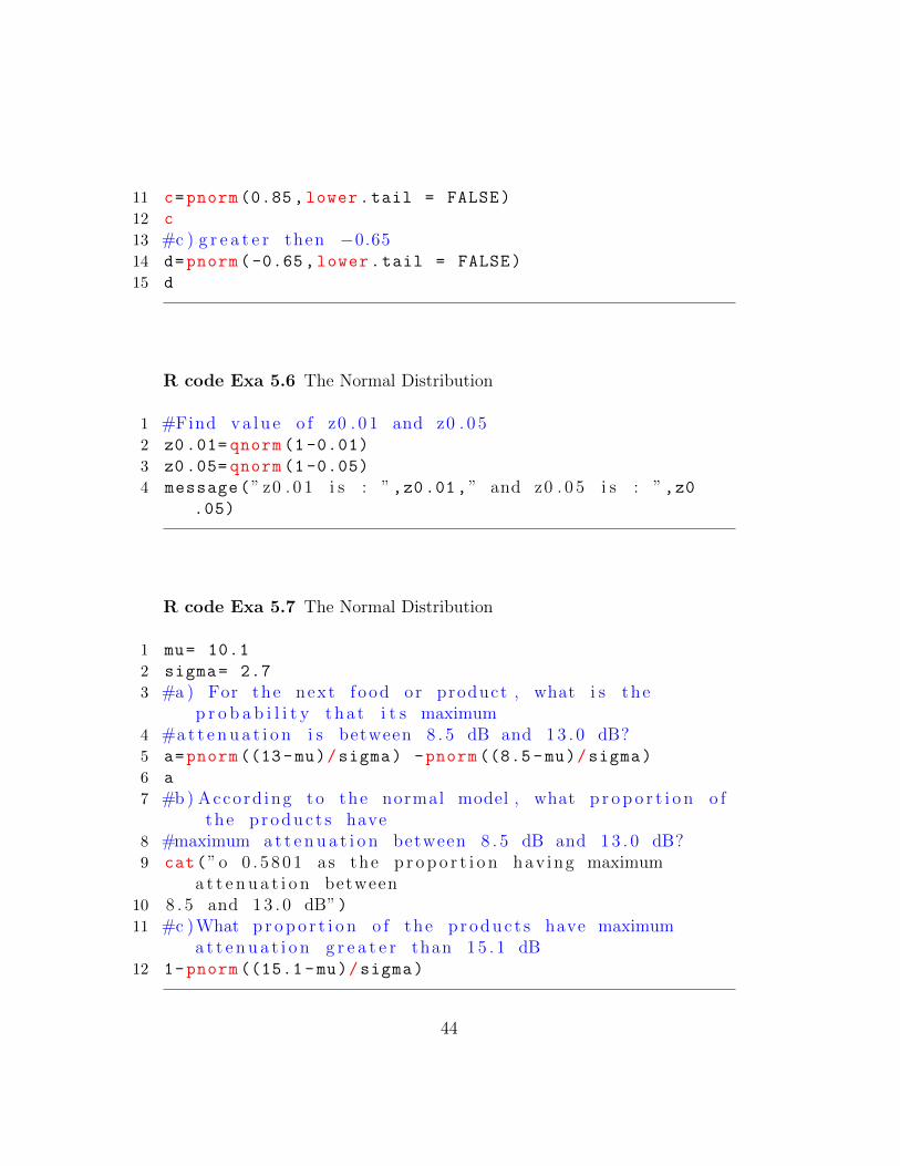
R code Exa 5.6 The Normal Distribution
1 #Find va lu e o f z0 . 0 1 and z0 . 0 52 z0.01= qnorm (1 -0.01)
3 z0.05= qnorm (1 -0.05)
4 message(” z0 . 0 1 i s : ”,z0.01,” and z0 . 0 5 i s : ”,z0.05)
R code Exa 5.7 The Normal Distribution
1 mu= 10.1
2 sigma= 2.7
3 #a ) For the next f ood or product , what i s thep r o b a b i l i t y tha t i t s maximum
4 #at t e nu a t i o n i s between 8 . 5 dB and 13 . 0 dB?5 a=pnorm ((13-mu)/sigma) -pnorm ((8.5 -mu)/sigma)
6 a
7 #b) Accord ing to the normal model , what p r op o r t i o n o fthe p roduc t s have
8 #maximum a t t e nu a t i o n between 8 . 5 dB and 13 . 0 dB?9 cat(”o 0 . 5 801 as the p r op o r t i o n hav ing maximum
a t t e nu a t i o n between10 8 . 5 and 13 . 0 dB”)11 #c )What p r op o r t i o n o f the p roduc t s have maximum
a t t e nu a t i o n g r e a t e r than 15 . 1 dB12 1-pnorm ((15.1 -mu)/sigma)
44
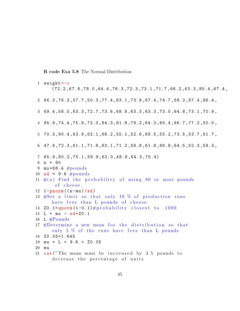
R code Exa 5.8 The Normal Distribution
1 weight <-c
(72.2 ,67.8 ,78.0 ,64.4 ,76.3 ,72.3 ,73.1 ,71.7 ,66.2 ,63.3 ,85.4 ,67.4 ,
2 66.3 ,76.3 ,57.7 ,50.3 ,77.4 ,63.1 ,73.9 ,67.4 ,74.7 ,68.2 ,87.4 ,86.4 ,
3 69.4 ,58.0 ,63.3 ,72.7 ,73.6 ,68.8 ,63.3 ,63.3 ,73.0 ,64.8 ,73.1 ,70.9 ,
4 85.9 ,74.4 ,75.9 ,72.3 ,84.3 ,61.8 ,79.2 ,64.3 ,65.4 ,66.7 ,77.2 ,50.0 ,
5 70.3 ,90.4 ,63.9 ,62.1 ,68.2 ,55.1 ,52.6 ,68.5 ,55.2 ,73.5 ,53.7 ,61.7 ,
6 47.9 ,72.3 ,61.1 ,71.8 ,83.1 ,71.2 ,58.8 ,61.8 ,86.8 ,64.5 ,52.3 ,58.3 ,
7 65.9 ,80.2 ,75.1 ,59.9 ,62.3 ,48.8 ,64.3 ,75.4)
8 n = 80
9 mu=68.4 #pounds10 sd = 9.6 #pounds11 #( a ) Find the p r o b a b i l i t y o f u s i n g 80 or more pounds
o f c h e e s e .12 1-pnorm((n-mu)/sd)
13 #Set a l i m i t so tha t on ly 10 % o f p r oduc t i on runshave l e s s than L pounds o f c h e e s e
14 Z0.1= qnorm (1 -0.1)#p r o b a b i l i t y c l o s e s t to . 1 0 0015 L = mu - sd*Z0.1
16 L #Pounds17 #Determine a new mean f o r the d i s t r i b u t i o n so tha t
on ly 5 % o f the runs have l e s s than L pounds18 Z0 .05=1.645
19 mu = L + 9.6 * Z0.05
20 mu
21 cat(”The mean must be i n c r e a s e d by 3 . 5 pounds tod e c r e a s e the p e r c en t a g e o f u n i t s
45
22 below the l i m i t L from 10% to 5%”)
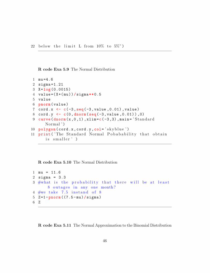
R code Exa 5.9 The Normal Distribution
1 mu=4.6
2 sigma =1.21
3 X=log (0.0015)
4 value=(X+(mu))/sigma**0.5
5 value
6 pnorm(value)
7 cord.x <- c(-3,seq(-3,value ,0.01) ,value)
8 cord.y <- c(0,dnorm(seq(-3,value ,0.01)) ,0)
9 curve(dnorm(x,0,1),xlim=c(-3,3),main= ’ StandardNormal ’ )
10 polygon(cord.x,cord.y,col= ’ s kyb lu e ’ )11 print( ’ The Standard Normal Pobabab i l i t y tha t ob t a i n
i s sma l l e r ’ )
R code Exa 5.10 The Normal Distribution
1 mu = 11.6
2 sigma = 3.3
3 #what i s the p r o b a b i l i t y tha t t h e r e w i l l be at l e a s t8 ou tag e s i n any one month?
4 #we take 7 . 5 i n s t and o f 85 Z=1-pnorm ((7.5-mu)/sigma)
6 Z
R code Exa 5.11 The Normal Approximation to the Binomial Distribution
46
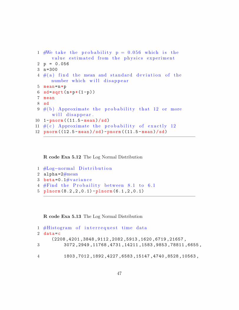
1 #We take the p r o b a b i l i t y p = 0 . 0 56 which i s theva lu e e s t ima t ed from the phy s i c s expe r iment
2 p = 0.056
3 n=300
4 #( a ) f i n d the mean and s tandard d e v i a t i o n o f thenumber which w i l l d i s a pp e a r
5 mean=n*p
6 sd=sqrt(n*p*(1-p))
7 mean
8 sd
9 #(b ) Approximate the p r o b a b i l i t y tha t 12 or morew i l l d i s a pp e a r .
10 1-pnorm ((11.5 - mean)/sd)
11 #( c ) Approximate the p r o b a b i l i t y o f e x a c t l y 1212 pnorm ((12.5 - mean)/sd)-pnorm ((11.5 - mean)/sd)
R code Exa 5.12 The Log Normal Distribution
1 #Log−normal D i s t r i b u t i o n2 alpha=2#mean3 beta =0.1#va r i a n c e4 #Find the P r o b a i l i t y between 8 . 1 to 6 . 15 plnorm (8.2 ,2 ,0.1)-plnorm (6.1 ,2 ,0.1)
R code Exa 5.13 The Log Normal Distribution
1 #Histogram o f i n t e r r e q u e s t t ime data2 data=c
(2208 ,4201 ,3848 ,9112 ,2082 ,5913 ,1620 ,6719 ,21657 ,
3 3072 ,2949 ,11768 ,4731 ,14211 ,1583 ,9853 ,78811 ,6655 ,
4 1803 ,7012 ,1892 ,4227 ,6583 ,15147 ,4740 ,8528 ,10563 ,
47
5 43003 ,16723 ,2613 ,26463 ,34867 ,4191 ,4030 ,2472 ,28840 ,
6 24487 ,14001 ,15241 ,1643 ,5732 ,5419 ,28608 ,2487 ,995 ,
7 3116 ,29508 ,11440 ,28336 ,3440
8 )
9 hist(data , freq = FALSE ,xlab = ”Time”)10 lines(density(data), col=” b lue ”, lwd =2)
R code Exa 5.14 The Log Normal Distribution
1 alpha=4
2 beta =0.3
3 a=33
4 #lo g norm p r o b a b i l i t y5 P=1-plnorm(a,alpha ,beta)
6 P
R code Exa 5.15 The Log Normal Distribution
1 alpha=2
2 beta =0.1
3 #mean4 mu=exp(1)^(alpha +(( beta)^2)/2)
5 mu
6 cat(”mean i s ”,mu)7 #va r i a n c e8 var=exp(1) ^((2*alpha+beta ^2))*(exp (1)^(beta ^2) -1)
9 var
10 cat(” v a r i a n c e i s ”,var)
48
R code Exa 5.16 The Gamma Distribution
1 data <-c
(0.894 ,0.991 ,0.061 ,0.186 ,0.311 ,0.817 ,2.267 ,0.091 ,0.139 ,0.083 ,
2 0.235 ,0.424 ,0.216 ,0.579 ,0.429 ,0.612 ,0.143 ,0.055 ,0.752 ,0.188 ,
3 0.071 ,0.195 ,0.082 ,1.653 ,2.010 ,0.158 ,0.527 ,1.033 ,2.863 ,0.365 ,
4 0.459 ,0.431 ,0.092 ,0.830 ,1.718 ,0.099 ,0.162 ,0.076 ,0.107 ,0.278 ,
5 0.100 ,0.919 ,0.900 ,0.093 ,0.041 ,0.712 ,0.994 ,0.149 ,0.866 ,0.054)
6 #decay Time i s r e p r e s e n t e d by h i s tog ram7 h<-hist(data , breaks =10, col=” red ”,xlab = ”
M i l l i s e c o n d ” ,prob = TRUE)
8 xfit <-seq(0,max(data),length =50)
9 yfit <-dnorm(xfit ,mean=mean(data),sd=sd(data))
10 yfit <- yfit*diff(h$mids [1:2])*length(data)
11 lines(xfit , yfit , col=” b lue ”, lwd =2)
R code Exa 5.17 The Gamma Distribution
1 f=function(x) 3*exp (1)^(-3*x)
2 #Assuming tha t the a r r i v a l f o l l o w po s s i o n p r o c e s swith a lpha=3 and beta=1/3
3 #a ) l e s s then 5 min4 integrate(f,lower = 0,upper = 1/12)
5 #b) at l e a s t 45 min6 integrate(f,lower = 3/4,upper = Inf)
R code Exa 5.18 The Beta Distribution
49
1 #beta d i s t r i b u t i o n2 #a )mean3 alpha=3
4 beta=2
5 mu=alpha/(alpha+beta)
6 mu
7 cat(”There f o r on ave rage ”,mu*100,”% highway s e c t i o nr e q u i r e r e p a i r e ”)
8 #b)9 F=pbeta(1/2,3,2)
10 plot(density(pbeta(seq(0,1/2,by=0.1) ,3,2)))
11 cat(”The p r o b a b i l i t y i s ”,F)
R code Exa 5.19 The Weibull Distribution
1 #we i b u l l d i s t r i b u t i o n2 scale =0.5
3 #mean l i f e t i m e4 mu =(0.1)**(-2)*factorial ((1+1/0.5) -1)
5 mu
6 #P(X>300)7 g=function(x)(0.05)*x^( -0.5)*exp (1)^(-0.1*x^scale)
8 integrate(g, lower = 300, upper = Inf)
R code Exa 5.20 Joint Distributions Discrete and Continuous
1 #P(X1+X2>1)2 P=0.2+0.1+0
3 message(” P r o b a b i l i t y i s : ”,P)4 #P( Xi=x i )5 p0 =0.1+0.2#p(X=0)6 p1 =0.4+0.2#p(X=1)7 p3 =0.1+0#p(X=2)
50
8 message(” P r o b a b i l i t s i s : ”)9 p0
10 p1
11 p3
R code Exa 5.21 Joint Distributions Discrete and Continuous
1 #Check the independency o f X1 and X22 #Cond i t i o n a l p r o b a b i l i t y3 #X2=14 #f ( 0 | 1 )5 f1=0.2/0.4#f ( 0 | 1 ) / f 2 ( 1 )6 #f ( 1 | 1 )7 f2=0.2/0.4#f ( 1 | 1 ) / f 2 ( 1 )8 #f ( 2 | 1 )9 f3=0/0.4#f ( 2 | 1 ) / f 2 ( 1 )
10 f1
11 f2
12 f3
13 message(” s i n c e f ( 0 | 1 ) != f 1 ( 0 ) t h e r e f o r i t ’ sdependent ”)
R code Exa 5.22 Joint Distributions Discrete and Continuous
1 llimy <- 2; llimx =1
2 ulimy <- 3 ; ulimx =2
3 #the f i r s t random v a r i a b l e w i l l t ake on a va lu ebetween 1 and 2 and the second
4 #random v a r i a b l e w i l l t ake on a va lu e between 2 and3
5 f <- function(x1 ,x2)6*exp (1)^(-2*x1 -3*x2)
6 integrate(function(x2) {
7 sapply(x2, function(x2) {
51
8 integrate(function(x1) f(x1,x2), llimx , ulimx)$
value
9 })
10 }, llimy , ulimy)
11 #(b ) the f i r s t random v a r i a b l e w i l l t ake on a va lu el e s s than 2 and the second
12 #random v a r i a b l e w i l l t ake on a va lu e g r e a t e r than 213 llimy <- 2; llimx =0
14 ulimy <- Inf ; ulimx=2
15 f <- function(x1 ,x2)6*exp (1)^(-2*x1 -3*x2)
16 integrate(function(x2) {
17 sapply(x2, function(x2) {
18 integrate(function(x1) f(x1,x2), llimx , ulimx)$
value
19 })
20 }, llimy , ulimy)
R code Exa 5.23 Joint Distributions Discrete and Continuous
1 F<-function(x,y){
2 return (1 - exp(1)^-2*x)*(1 - exp (1)^-3*y)
3 }
4 F(1,1)
R code Exa 5.31 Joint Distributions Discrete and Continuous
1 EX1=4
2 EX2=-2
3 VX1=9
4 VX2=6
5 #Ca l cua t i on6 cat(”E( 2X1+X2−5 ) = ” ,2*EX1+EX2 -5)7 cat(”Var (2X1+X2−5 ) = ” ,2^2*VX1+VX2)
52
R code Exa 5.42 Checking If the Data Are Normal
1 # Normal S c o r e s p l o t o f no rma l i z ed data2 Score=c(67, 48, 76, 81)
3 qqnorm(Score , ylab=”Ordered o b s e r v a t i o n s ”, xlab=”Normal S c o r e s ”, main=””)
R code Exa 5.43 Transforming Observations to Near Normality
1 #Histogram to Normal S c o r e s p l o t o f no rma l i z ed data2 data=c
(2208 ,4201 ,3848 ,9112 ,2082 ,5913 ,1620 ,6719 ,21657 ,
3 3072 ,2949 ,11768 ,4731 ,14211 ,1583 ,9853 ,78811 ,6655 ,
4 1803 ,7012 ,1892 ,4227 ,6583 ,15147 ,4740 ,8528 ,10563 ,
5 43003 ,16723 ,2613 ,26463 ,34867 ,4191 ,4030 ,2472 ,28840 ,
6 24487 ,14001 ,15241 ,1643 ,5732 ,5419 ,28608 ,2487 ,995 ,
7 3116 ,29508 ,11440 ,28336 ,3440
8 )
9 hist(data ,ylab=” C l a s s f r e qu en cy ”, xlab=” t ime ”)10 qqnorm(data , ylab=” I n t e r r q u e s t t ime ”, xlab=”Normal
S c o r e s ”, main=””)11 ln=log(data)
12 hist(ln,ylab=” C l a s s f r e qu en cy ”, xlab=” l n ( t ime ) ”)13 qqnorm(ln, ylab=” l n ( I n t e r r q u e s t t ime ) ”, xlab=”Normal
S c o r e s ”, main=””)
R code Exa 5.44 Simulation
1 Data <-c(0.57 ,0.74 ,0.26 ,0.77 ,0.12)
53
2 alpha = 0.05
3 beta = 2.0
4 ((-1/alpha)*log(1-Data))^(1/beta)
R code Exa 5.45 Simulation
1 mu=50
2 sigma=5
3 u1 =0.253
4 u2 =0.531
5 #standard normal v a l u e s6 z1=(-2*log(u2))**0.5*cos(2*pi*u1)
7 z1
8 z2=(-2*log(u2))**0.5*sin(2*pi*u1)
9 z2
10 #normal va l u e11 x1=50+5*z1
12 x2=50+5*z2
13 x1
14 x2
54
Chapter 6
SAMPLING DISTRIBUTIONS
R code Exa 6.49 The Sampling Distribution of the Mean
1 #Find the popu l a t i o n c o r r e c t i o n f a c t o r2 #Given3 n=10
4 N=1000
5 factor =(N-n)/(N-1)
6 message(”There f o r the f a c t o r i s : ”,factor)
R code Exa 6.51 The Sampling Distribution of the Mean
1 #sampl ing d i s t r i b u t i o n2 options(digits = 3)
3 sd=1.20
4 mean =1.82#mean5 n=40
6 Xbar <-c(1.65 ,2.04)
7 Xbar
8 z=(Xbar -mean)*(n**0.5)/(sd)
9 z
55
10 message(” P r o b a b i l i t y i s : ”,pnorm (1.16) -pnorm ( -0.896))
R code Exa 6.52 The Sampling Distribution of the Mean Sigma Unknown
1 n = 20
2 mu=40 #mg/ l3 xbar = 46
4 s = 9.4 #mg/ l5 df=n-1
6 t0.01=qt(1-0.01,df)
7 t0.01
8 t=(xbar -mu)/(s/n^0.5)
9 message(” t va lu e i s : ”,t)10 P=1 - pt(t,19)
11 message(” p r o b a b i l i t y i s : ”,P)12 print(” S i n c e s the t va l u e exceed t0 . 0 1 t h e r e f o r we
r e j e c t the c l a im ”)
R code Exa 6.53 The Sampling Distribution of the Variance
1 var =1.35#popu l a t i o n v a r i a n c e2 s=1.4#sample v a r i a n c e3 n=20#t o t a l no o f sample4 chi =((n+2)*1.4*1.4)/1.2^2
5 ceiling(chi)
6 qchisq (1 -0.05 ,19)
7 1 -pchisq (30.6 , 19)
8 cat(”There f o r the p r o b a b i l i t y tha t a good shipmeant9 w i l l e r r o n e o u s l y be r e j e c t i s l e s s then 0 . 0 5 ”)
56
R code Exa 5.54 The Sampling Distribution of the Variance
1 #Random sample s i z e2 n1=7
3 n2=13
4 #th e r e f o r numerator and denominator d eg r e e o ff reedom i s
5 v1=n1 -1
6 v2=n2 -1
7 1/df(0.05,v1,v2)
8 F0.05=qf(1 -0.05 ,6 ,12)
9 F0.05
10 print(”There f o r the p r o b a b i l i t y i s 0 . 0 5 ”)
R code Exa 6.55 The Sampling Distribution of the Variance
1 #F d i s t r i b u t i o n2 #l e f t −hand t a i l p r o b a b i l i t y3 #a ) by f i r s t method4 df1 =20#f i r s t d e g r e e o f f reedom5 df2 =10#second deg r e e o f f reedom6 data=qf(0.95,df1 ,df2)#qu a n t i l e7 Area=1/data
8 cat(”Value under th a r ea 0 . 9 5 i s ”,Area)
57
Chapter 7
Inferences Concerning a Mean
R code Exa 7.2 Point Estimation
1 Data <-c(136 ,143 ,147 ,151 ,158 ,160 ,
2 161 ,163 ,165 ,167 ,173 ,174 ,
3 181 ,181 ,185 ,188 ,190 ,205)
4 Xbar=mean(Data)
5 s=sd(Data)
6 #standard e r r o r i s7 E=s/sqrt(length(Data))
8 E
R code Exa 7.3 Point Estimation
1 n=150
2 sigma =6.2
3 Z0 .05=2.575
4 E=sigma*Z0.05/sqrt(n)
5 E
6 message(”Thus , the e n g i n e e r can a s s e r t withp r o b a b i l i t y 0 . 9 9 tha t h i s e r r o r w i l l be at
7 most 1 . 3 0 . ”)
58
R code Exa 7.4 Point Estimation
1 # 98% c on f i d e n c e about the maximum e r r o r ?2 n = 6
3 s = 1.14
4 t0.01 =qt(1 -0.01 ,5)
5 E=t0.01*s/sqrt(n)
6 E
7 message(”Thus the chemi s t can a s s e r t with 98%c on f i d e n c e tha t h i s f i g u r e f o r the me l t i ng po i n t
8 o f the aluminum a l l o y i s o f f by at most 1 . 566049d e g r e e s ”)
R code Exa 7.5 Point Estimation
1 E = 0.50
2 sigma = 1.6
3 z0.025 = 1.96
4 n=(sigma*z0.025/E)^2
5 n
6 message(”Thus , the r e s e a r c h worker w i l l have to t ime40 mechan ics p e r f o rm ing the t a sk o f
7 r o t a t i n g the t i r e s o f a ca r ”)
R code Exa 7.6 Interval Estimation
1 n=100#random sample o f s i z e2 sigma =5.1
3 xbar =21.6
59
4 z0 .025=1.96
5 #the r f o r 95% c o n f i d e n c e i n t e r v a l f o r the popu l a t i o nmean i s
6 Int1=xbar -z0.025*(sigma/sqrt(n))
7 Int2=xbar+z0.025*(sigma/sqrt(n))
8 cat(”There f o r c o n f i d e n c e i n t e r v a l mean i s : ”,Int1 ,”< ”,Int2)
R code Exa 7.7 Interval Estimation
1 n =50
2 x = 305.58#nm3 var = 1366.86
4 s = 36.97#nm5 #con s t r u c t a 99% c on f i d e n c e i n t e r v a l f o r the
popu l a t i o n mean o f a l l n a n o p i l l a r s6 z0.005 = 2.575
7 Int1=x-z0.005*(s/sqrt(n))
8 Int1
9 Int2=x+z0.005*(s/sqrt(n))
10 Int2
11 message(”There f o r the c o n f i d e n c e i n t e r v a l i s : ”,Int1 ,” < ”,Int2)
R code Exa 7.8 Interval Estimation
1 n = 18
2 x = 22.6
3 s = 15.7
4 t0.025=qt(1 -0.025 ,17)
5 Int1=x-t0.025*s/sqrt(n)
6 Int1
7 Int2=x+t0.025*s/sqrt(n)
60
8 Int2
9 cat(”We ar e 95 % c o n f i d e n t tha t the i n t e r v a l from14 . 7 9 to 30 . 4 1 MJ/m3 con t a i n s the
10 mean toughne s s o f a l l p o s s i b l e a r t i f i c i a l f i b e r sc r e a t e d by the c u r r e n t p r o c e s s . ”)
R code Exa 7.13 Maximum Likelihood Estimation
1 #Po i s s on d i s t r i b u t i o n o f d e f e c t i v e hard d r i v e f o rten day
2 Data <-c(7,3,1,2,4,1,2,3,1,2)
3 T=sum(Data)
4 lamda=T/10
5 #the maximum l i k e l i h o o d e s t ima t e i s6 #P(X=0 or 1)7 P=exp(1)^(-lamda)+( lamda*exp(1)^(-lamda))
8 P
9 cat(”There f o r t h e r e w i l l be 1 or f ewe r d e f e c t i v e son j u s t ove r one−qua r t e r o f the days . ”)
R code Exa 7.15 Maximum Likelihood Estimation
1 #The y i e l d s o f ch em i ca l r e c t i o n i s as2 op<-c(5.57 ,5.76 ,4.18 ,4.64 ,7.02 ,6.62 ,6.33 ,7.24 ,
3 5.57 ,7.89 ,4.67 ,7.24 ,6.43 ,5.59 ,5.39)
4 #( a ) Obtain the maximum l i k e l i h o o d e s t ima t e s o f themean y i e l d and the v a r i a n c e
5 mean=mean(op)
6 cat(mean ,” g a l ”)7 var =(1/length(op))*sum((op -mean)^2)
8 var
9 #Obtain the maximum l i k e l i h o o d e s t ima t e o f thec o e f f i c i e n t o f v a r i a t i o n ?? / ??
61
10 cat(” c o e f f i c i e n t i s : ”,sqrt(var)/mean)
R code Exa 7.18 Hypotheses Concerning One Mean
1 xbar =3.9
2 mu=4.5
3 sigma =1.5
4 n=25
5 Z=(xbar -mu)/(sigma/sqrt(n))
6 Z
7 P=pnorm(Z)
8 P
9 cat(”There the p r o b a b i l i t y tha t the va l u e o f z i s −2i s 0 . 0 227 ”)
10 message(”There f o r the p va lu e i s : ” ,2*P)
R code Exa 7.19 Hypotheses Concerning One Mean
1 xbar = 68.45
2 s = 9.583
3 mu=71
4 #Nul l h yp o t h e s i s : mu = 71 pounds5 #A l t e r n a t i v e h yp o t h e s i s : mu < 71 pounds6 z.alpha=qnorm (0.01)
7 #Cr i t e r i o n : S i n c e the p r o b a b i l i t y o f a Type I e r r o ri s g r e a t e s t when mu = 71
8 #pounds , we proce ed as i f we were t e s t i n g the n u l lh yp o t h e s i s mu = 71 pounds
9 #aga i n s t the a l t e r n a t i v e h yp o t h e s i s mu < 71 poundsat the 0 . 0 1 l e v e l o f
10 #s i g n i f i c a n c e . Thus , the n u l l h yp o t h e s i s must ber e j e c t e d i f Z < −2.33 , where
11 Z=(xbar -mu)/(s/sqrt (80))
62
12 Z
13 #Dec i s i o n : S i n c e Z = −2.38 i s l e s s than −2.33 , then u l l h yp o t h e s i s must be
14 #r e j e c t e d at l e v e l o f s i g n i f i c a n c e 0 . 0 1 . In o th e rwords , the s u s p i c i o n tha t mu < 71
15 #pounds i s con f i rmed .
R code Exa 7.20 Hypotheses Concerning One Mean
1 #measurements o f l e ad con t en t ( ?? g / L) a r e takenfrom twe l v e water spec imens sp i k ed with a knownc o n c e n t r a t i o n
2 data <-c
(2.4 ,2.9 ,2.7 ,2.6 ,2.9 ,2.0 ,2.8 ,2.2 ,2.4 ,2.4 ,2.0 ,2.5)
3 x = 2.483
4 s = 0.3129
5 #Nul l h yp o t h e s i s : mu = 2 . 2 5 mig/L6 #A l t e r n a t i v e h yp o t h e s i s : mu > 2 . 2 5 mig/L7 mu=2.25
8 #Cr i t e r i o n : Re j e c t the n u l l h yp o t h e s i s i f t > 2 . 2 0 1 ,where 2 . 2 01 i s the va lu e o f
9 #t0 . 0 2 5 f o r 12−1 = 11 d e g r e e s o f f reedom10 t0.025=qt(1 -0.025 ,11)
11 t.test(data ,mu=2.25 , alt= ’ g r e a t e r ’ ,conf =.95)12 cat(” De c i s i o n : S i n c e t = 2 . 5 8 i s g r e a t e r than 2 . 2 0 1 ,
the n u l l h yp o t h e s i s must13 be r e j e c t e d . In o th e r words , the mean l e ad con t en t
i s above14 2 . 2 5 mig/L . ”)
R code Exa 7.22 Power Sample Size and Operating Characteristic Curves
1 sd=3.6#dB
63
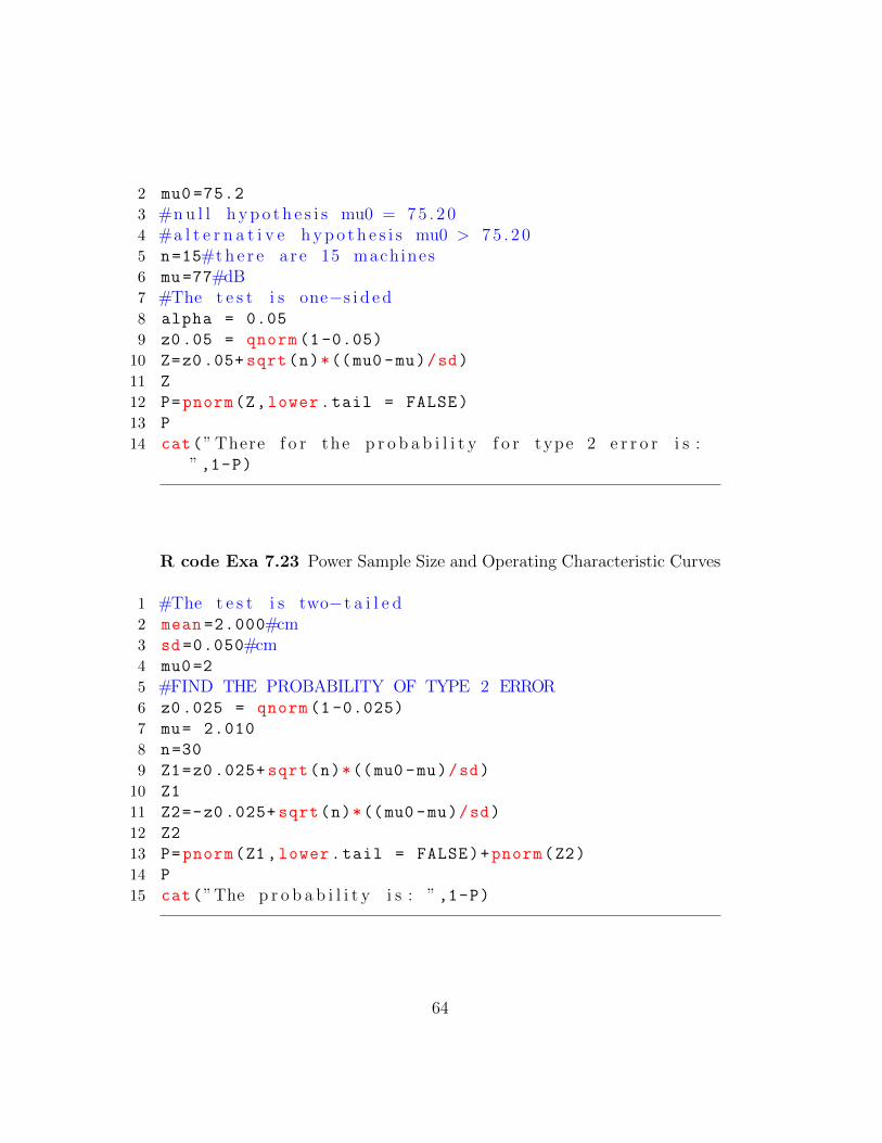
2 mu0 =75.2
3 #nu l l h yp o t h e s i s mu0 = 75 . 2 04 #a l t e r n a t i v e h yp o t h e s i s mu0 > 75 . 2 05 n=15#th e r e a r e 15 machines6 mu=77#dB7 #The t e s t i s one−s i d e d8 alpha = 0.05
9 z0.05 = qnorm (1 -0.05)
10 Z=z0.05+ sqrt(n)*((mu0 -mu)/sd)
11 Z
12 P=pnorm(Z,lower.tail = FALSE)
13 P
14 cat(”There f o r the p r o b a b i l i t y f o r type 2 e r r o r i s :” ,1-P)
R code Exa 7.23 Power Sample Size and Operating Characteristic Curves
1 #The t e s t i s two−t a i l e d2 mean =2.000#cm3 sd =0.050#cm4 mu0=2
5 #FIND THE PROBABILITY OF TYPE 2 ERROR6 z0.025 = qnorm (1 -0.025)
7 mu= 2.010
8 n=30
9 Z1=z0 .025+ sqrt(n)*((mu0 -mu)/sd)
10 Z1
11 Z2=-z0 .025+ sqrt(n)*((mu0 -mu)/sd)
12 Z2
13 P=pnorm(Z1,lower.tail = FALSE)+pnorm(Z2)
14 P
15 cat(”The p r o b a b i l i t y i s : ” ,1-P)
64
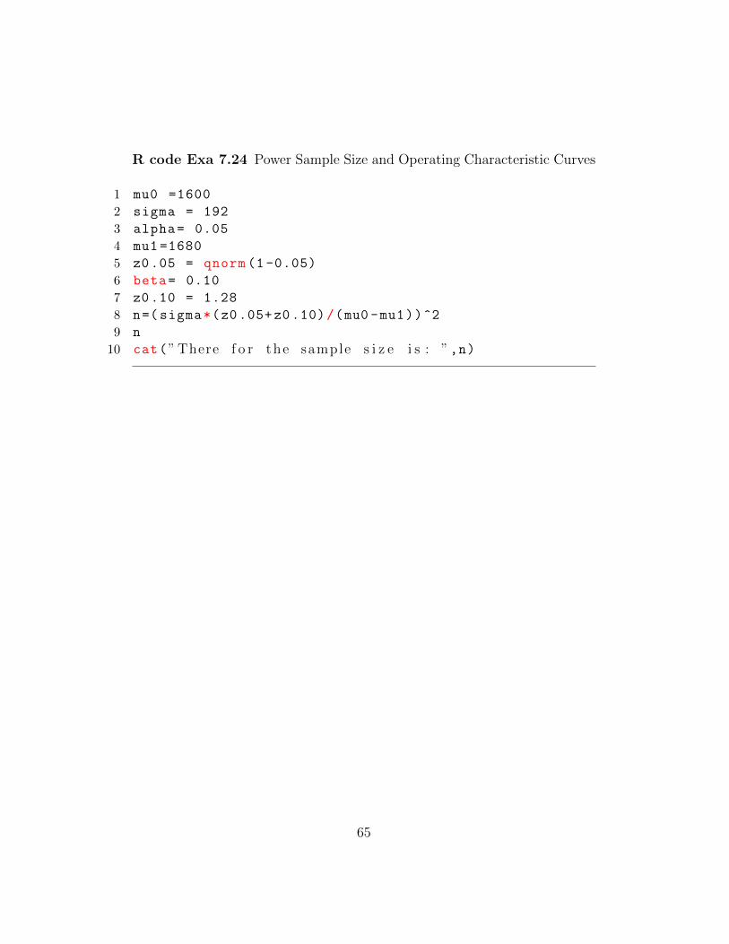
R code Exa 7.24 Power Sample Size and Operating Characteristic Curves
1 mu0 =1600
2 sigma = 192
3 alpha= 0.05
4 mu1 =1680
5 z0.05 = qnorm (1 -0.05)
6 beta= 0.10
7 z0.10 = 1.28
8 n=(sigma*(z0.05+z0.10)/(mu0 -mu1))^2
9 n
10 cat(”There f o r the sample s i z e i s : ”,n)
65
Chapter 8
Comparing Two Treatments
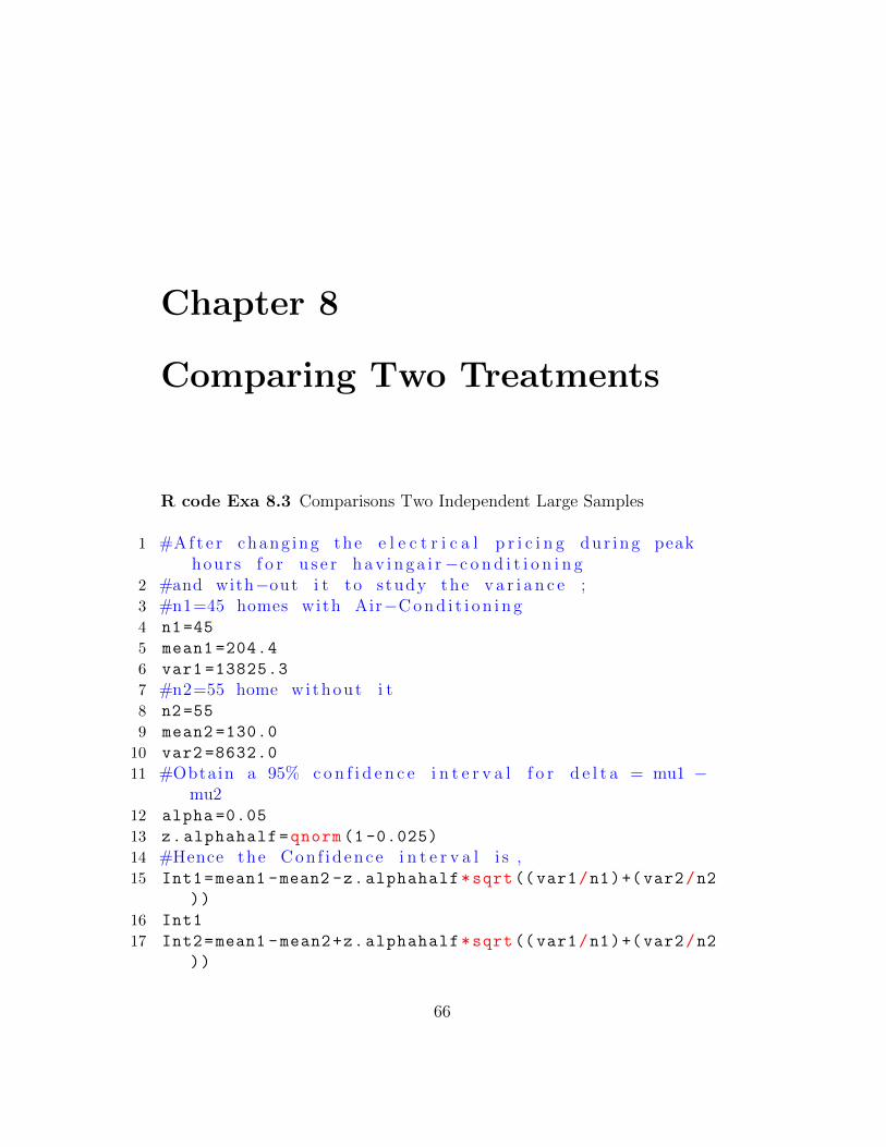
R code Exa 8.3 Comparisons Two Independent Large Samples
1 #Af t e r chang ing the e l e c t r i c a l p r i c i n g dur ing peakhours f o r u s e r hav i nga i r−c o n d i t i o n i n g
2 #and with−out i t to s tudy the v a r i a n c e ;3 #n1=45 homes with Air−Cond i t i on i n g4 n1=45
5 mean1 =204.4
6 var1 =13825.3
7 #n2=55 home wi thout i t8 n2=55
9 mean2 =130.0
10 var2 =8632.0
11 #Obtain a 95% c on f i d e n c e i n t e r v a l f o r d e l t a = mu1 −mu2
12 alpha =0.05
13 z.alphahalf=qnorm (1 -0.025)
14 #Hence the Con f i d ence i n t e r v a l i s ,15 Int1=mean1 -mean2 -z.alphahalf*sqrt((var1/n1)+(var2/n2
))
16 Int1
17 Int2=mean1 -mean2+z.alphahalf*sqrt((var1/n1)+(var2/n2
))
66
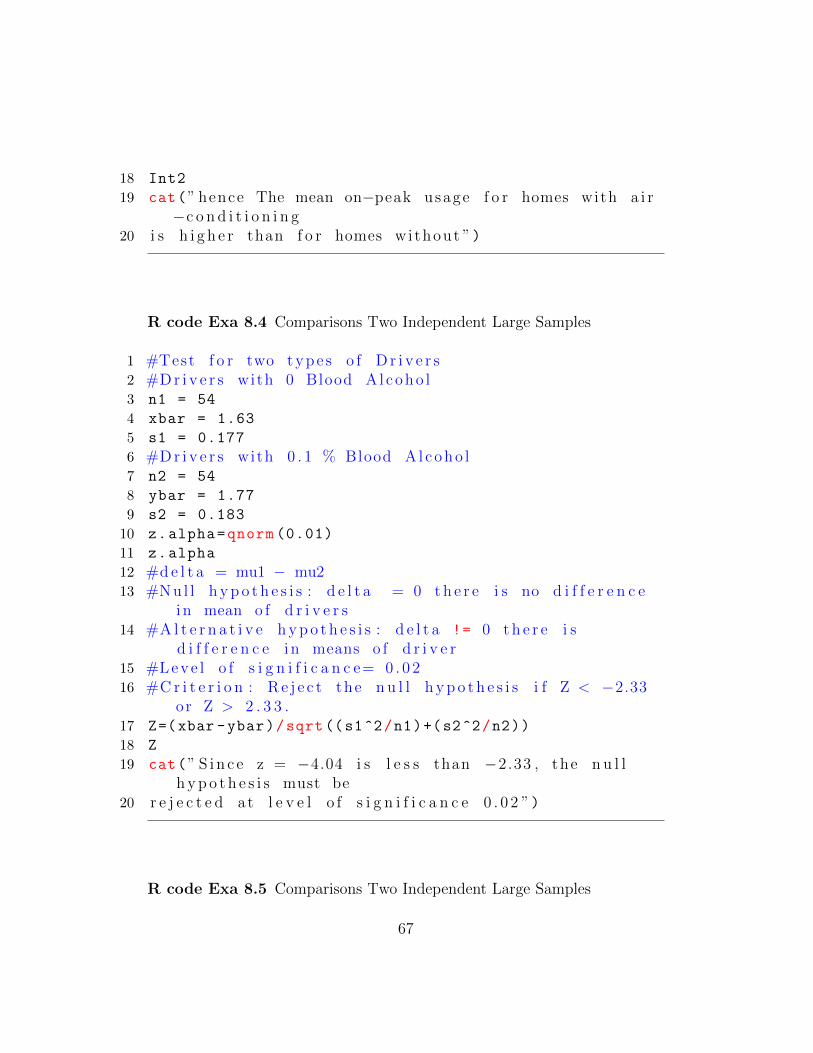
18 Int2
19 cat(” hence The mean on−peak usage f o r homes with a i r−c o n d i t i o n i n g
20 i s h i g h e r than f o r homes wi thout ”)
R code Exa 8.4 Comparisons Two Independent Large Samples
1 #Test f o r two type s o f D r i v e r s2 #Dr i v e r s with 0 Blood A l coho l3 n1 = 54
4 xbar = 1.63
5 s1 = 0.177
6 #Dr i v e r s with 0 . 1 % Blood A l coho l7 n2 = 54
8 ybar = 1.77
9 s2 = 0.183
10 z.alpha=qnorm (0.01)
11 z.alpha
12 #de l t a = mu1 − mu213 #Nul l h yp o t h e s i s : d e l t a = 0 t h e r e i s no d i f f e r e n c e
i n mean o f d r i v e r s14 #A l t e r n a t i v e h yp o t h e s i s : d e l t a != 0 t h e r e i s
d i f f e r e n c e i n means o f d r i v e r15 #Leve l o f s i g n i f i c a n c e= 0 . 0 216 #Cr i t e r i o n : Re j e c t the n u l l h yp o t h e s i s i f Z < −2.33
or Z > 2 . 3 3 .17 Z=(xbar -ybar)/sqrt((s1^2/n1)+(s2^2/n2))
18 Z
19 cat(” S i n c e z = −4.04 i s l e s s than −2.33 , the n u l lh yp o t h e s i s must be
20 r e j e c t e d at l e v e l o f s i g n i f i c a n c e 0 . 0 2 ”)
R code Exa 8.5 Comparisons Two Independent Large Samples
67
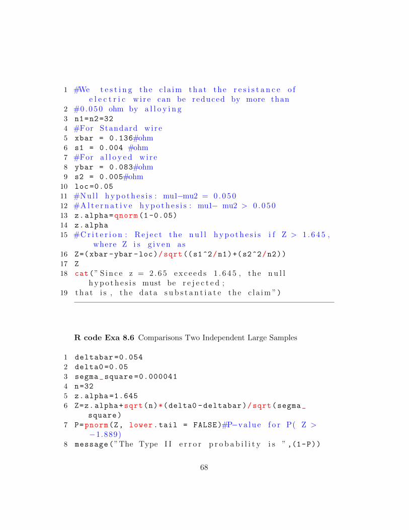
1 #We t e s t i n g the c l a im tha t the r e s i s t a n c e o fe l e c t r i c w i r e can be reduced by more than
2 #0 . 050 ohm by a l l o y i n g3 n1=n2=32
4 #For Standard w i r e5 xbar = 0.136#ohm6 s1 = 0.004 #ohm7 #For a l l o y e d w i r e8 ybar = 0.083#ohm9 s2 = 0.005#ohm10 loc =0.05
11 #Nul l h yp o t h e s i s : mu1−mu2 = 0 . 05012 #A l t e r n a t i v e h yp o t h e s i s : mu1− mu2 > 0 . 0 5013 z.alpha=qnorm (1 -0.05)
14 z.alpha
15 #Cr i t e r i o n : Re j e c t the n u l l h yp o t h e s i s i f Z > 1 . 6 4 5 ,where Z i s g i v en as
16 Z=(xbar -ybar -loc)/sqrt((s1^2/n1)+(s2^2/n2))
17 Z
18 cat(” S i n c e z = 2 . 6 5 ex c e ed s 1 . 6 4 5 , the n u l lh yp o t h e s i s must be r e j e c t e d ;
19 tha t i s , the data s u b s t a n t i a t e the c l a im ”)
R code Exa 8.6 Comparisons Two Independent Large Samples
1 deltabar =0.054
2 delta0 =0.05
3 segma_square =0.000041
4 n=32
5 z.alpha =1.645
6 Z=z.alpha+sqrt(n)*(delta0 -deltabar)/sqrt(segma_
square)
7 P=pnorm(Z, lower.tail = FALSE)#P−va lu e f o r P( Z >−1.889)
8 message(”The Type I I e r r o r p r o b a b i l i t y i s ” ,(1-P))
68
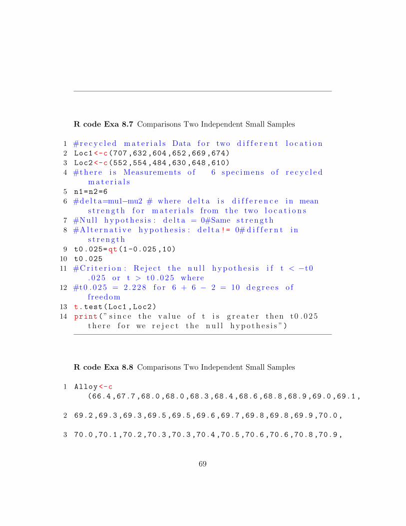
R code Exa 8.7 Comparisons Two Independent Small Samples
1 #r e c y c l e d ma t e r i a l s Data f o r two d i f f e r e n t l o c a t i o n2 Loc1 <-c(707 ,632 ,604 ,652 ,669 ,674)
3 Loc2 <-c(552 ,554 ,484 ,630 ,648 ,610)
4 #th e r e i s Measurements o f 6 spec imens o f r e c y c l e dma t e r i a l s
5 n1=n2=6
6 #de l t a=mu1−mu2 # where d e l t a i s d i f f e r e n c e i n means t r e n g t h f o r ma t e r i a l s from the two l o c a t i o n s
7 #Nul l h yp o t h e s i s : d e l t a = 0#Same s t r e n g t h8 #A l t e r n a t i v e h yp o t h e s i s : d e l t a != 0#d i f f e r n t i n
s t r e n g t h9 t0.025=qt(1 -0.025 ,10)
10 t0.025
11 #Cr i t e r i o n : Re j e c t the n u l l h yp o t h e s i s i f t < −t0. 0 2 5 or t > t0 . 0 2 5 where
12 #t0 . 0 2 5 = 2 . 2 28 f o r 6 + 6 − 2 = 10 d e g r e e s o ff reedom
13 t.test(Loc1 ,Loc2)
14 print(” s i n c e the va l u e o f t i s g r e a t e r then t0 . 0 2 5t h e r e f o r we r e j e c t the n u l l h yp o t h e s i s ”)
R code Exa 8.8 Comparisons Two Independent Small Samples
1 Alloy <-c
(66.4 ,67.7 ,68.0 ,68.0 ,68.3 ,68.4 ,68.6 ,68.8 ,68.9 ,69.0 ,69.1 ,
2 69.2 ,69.3 ,69.3 ,69.5 ,69.5 ,69.6 ,69.7 ,69.8 ,69.8 ,69.9 ,70.0 ,
3 70.0 ,70.1 ,70.2 ,70.3 ,70.3 ,70.4 ,70.5 ,70.6 ,70.6 ,70.8 ,70.9 ,
69
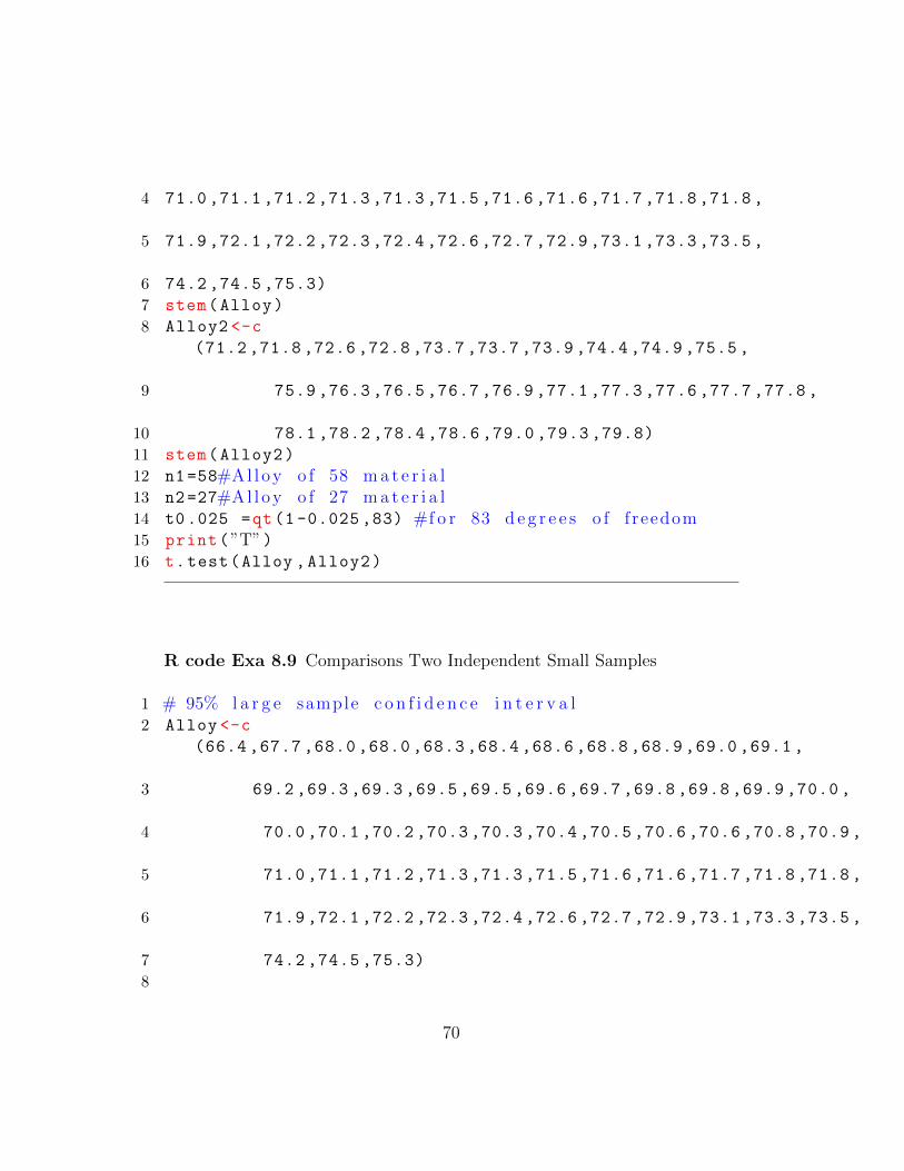
4 71.0 ,71.1 ,71.2 ,71.3 ,71.3 ,71.5 ,71.6 ,71.6 ,71.7 ,71.8 ,71.8 ,
5 71.9 ,72.1 ,72.2 ,72.3 ,72.4 ,72.6 ,72.7 ,72.9 ,73.1 ,73.3 ,73.5 ,
6 74.2 ,74.5 ,75.3)
7 stem(Alloy)
8 Alloy2 <-c
(71.2 ,71.8 ,72.6 ,72.8 ,73.7 ,73.7 ,73.9 ,74.4 ,74.9 ,75.5 ,
9 75.9 ,76.3 ,76.5 ,76.7 ,76.9 ,77.1 ,77.3 ,77.6 ,77.7 ,77.8 ,
10 78.1 ,78.2 ,78.4 ,78.6 ,79.0 ,79.3 ,79.8)
11 stem(Alloy2)
12 n1=58#Al l oy o f 58 ma t e r i a l13 n2=27#Al l oy o f 27 ma t e r i a l14 t0.025 =qt(1 -0.025 ,83) #f o r 83 d e g r e e s o f f reedom15 print(”T”)16 t.test(Alloy ,Alloy2)
R code Exa 8.9 Comparisons Two Independent Small Samples
1 # 95% l a r g e sample c o n f i d e n c e i n t e r v a l2 Alloy <-c
(66.4 ,67.7 ,68.0 ,68.0 ,68.3 ,68.4 ,68.6 ,68.8 ,68.9 ,69.0 ,69.1 ,
3 69.2 ,69.3 ,69.3 ,69.5 ,69.5 ,69.6 ,69.7 ,69.8 ,69.8 ,69.9 ,70.0 ,
4 70.0 ,70.1 ,70.2 ,70.3 ,70.3 ,70.4 ,70.5 ,70.6 ,70.6 ,70.8 ,70.9 ,
5 71.0 ,71.1 ,71.2 ,71.3 ,71.3 ,71.5 ,71.6 ,71.6 ,71.7 ,71.8 ,71.8 ,
6 71.9 ,72.1 ,72.2 ,72.3 ,72.4 ,72.6 ,72.7 ,72.9 ,73.1 ,73.3 ,73.5 ,
7 74.2 ,74.5 ,75.3)
8
70
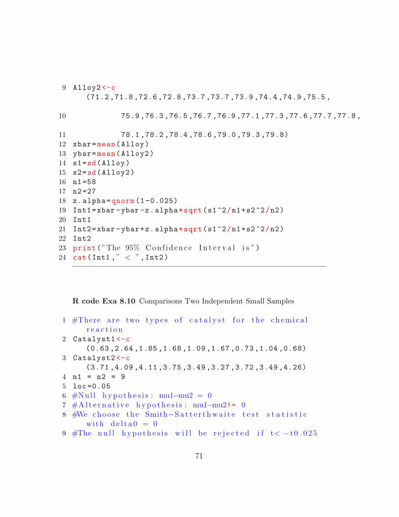
9 Alloy2 <-c
(71.2 ,71.8 ,72.6 ,72.8 ,73.7 ,73.7 ,73.9 ,74.4 ,74.9 ,75.5 ,
10 75.9 ,76.3 ,76.5 ,76.7 ,76.9 ,77.1 ,77.3 ,77.6 ,77.7 ,77.8 ,
11 78.1 ,78.2 ,78.4 ,78.6 ,79.0 ,79.3 ,79.8)
12 xbar=mean(Alloy)
13 ybar=mean(Alloy2)
14 s1=sd(Alloy)
15 s2=sd(Alloy2)
16 n1=58
17 n2=27
18 z.alpha=qnorm (1 -0.025)
19 Int1=xbar -ybar -z.alpha*sqrt(s1^2/n1+s2^2/n2)
20 Int1
21 Int2=xbar -ybar+z.alpha*sqrt(s1^2/n1+s2^2/n2)
22 Int2
23 print(”The 95% Con f id ence I n t e r v a l i s ”)24 cat(Int1 ,” < ”,Int2)
R code Exa 8.10 Comparisons Two Independent Small Samples
1 #There a r e two type s o f c a t a l y s t f o r the chem i ca lr e a c t i o n
2 Catalyst1 <-c
(0.63 ,2.64 ,1.85 ,1.68 ,1.09 ,1.67 ,0.73 ,1.04 ,0.68)
3 Catalyst2 <-c
(3.71 ,4.09 ,4.11 ,3.75 ,3.49 ,3.27 ,3.72 ,3.49 ,4.26)
4 n1 = n2 = 9
5 loc =0.05
6 #Nul l h yp o t h e s i s : mu1−mu2 = 07 #A l t e r n a t i v e h yp o t h e s i s : mu1−mu2!= 08 #We choose the Smith−S a t t e r t hwa i t e t e s t s t a t i s t i c
with d e l t a 0 = 09 #The n u l l h yp o t h e s i s w i l l be r e j e c t e d i f t< −t0 . 0 2 5
71
or t > t0 . 0 2 5 , but the va lu e10 #o f t0 . 0 2 5 depends on the e s t ima t ed d e g r e e s o f
f reedom .11 df=11
12 t0.025=qt(1 -0.025 ,11)
13 t0.025
14 t.test(Catalyst1 ,Catalyst2 ,alternative =”g”)15 cat(” De c i s i o n : S i n c e t= −9.71 i s l e s s than −2.201 ,
the n u l l h yp o t h e s i s must be16 r e j e c t e d at l e v e l o f s i g n i f i c a n c e 0 . 0 5 ”)
R code Exa 8.11 Comparisons Two Independent Small Samples
1 #There a r e two type s o f c a t a l y s t f o r the chem i ca lr e a c t i o n
2 Catalyst1 <-c
(0.63 ,2.64 ,1.85 ,1.68 ,1.09 ,1.67 ,0.73 ,1.04 ,0.68)
3 Catalyst2 <-c
(3.71 ,4.09 ,4.11 ,3.75 ,3.49 ,3.27 ,3.72 ,3.49 ,4.26)
4 # 95% c on f i d e n c e i n t e r v a l f o r d e l t a = mu1 − mu25 x =mean(Catalyst1)
6 s1 = sd(Catalyst1)
7 y =mean(Catalyst2)
8 s2=sd(Catalyst2)
9 df=11
10 t0.025 =qt(1 -0.025,df)
11 t.test(Catalyst1 ,Catalyst2)
12 cat(”The mean product volume f o r the second c a t a l y s ti s
13 g r e a t e r than tha t o f the f i r s t c a t a l y s t by 1 . 8 80 to2 . 9 82 g a l l o n s ”)
R code Exa 8.12 Matched Pairs Comparisons
72
1 before <-c(45 ,73 ,46 ,124 ,33 ,57 ,83 ,34 ,26 ,17)
2 After <-c(36 ,60 ,44 ,119 ,35 ,51 ,77 ,29 ,24 ,11)
3 #Nul l Hypo the s i s :mu=0#There i s no d i f f e r e n c e i n meano f data t h e r e f o r the program i s not e f f e c t i v e
4 #A l t e r n a t i v e h yp o t h e s i s : mu>0 the program i se f f e c t i v e
5 l.o.c=0.05
6 t0.05=qt(1 -0.05 ,9)
7 t0.05
8 #Cr i t e r i o n : Re j e c t Nu l l Hypo the s i s i f t>t0 . 0 5 or1 . 8 33 f o r d f=9
9 #t c a l c u l a t i o n10 t.test(before ,After ,paired=TRUE)
11 print(” hence we r e j e c t Nu l l h yp o t h e s i s because t>t0. 0 5 ”)
12 print(”There f o r the s a f e t y program i s e f f e c t i v e ”)
R code Exa 8.13 Matched Pairs Comparisons
1 #measurment o f t o x i c l e v e l o f ch em i ca l2 data <-c(1.26 ,1.34 ,1.82 ,0.55 ,0.73 ,0.78 ,1.10)
3 n = 7 #Sample s i z e4 t.alpha=qt(1 -0.025 ,6)
5 # the 95% c on f i d e n c e fo rmu la f o r mu becomes6 t.test(data)
7 cat(”We ar e 95% c o n f i d e n t tha t the i n t e r v a l from0 . 6 8 to 1 . 4 9
8 c o n t a i n s the mean change i n the red c o l o r component ”)
R code Exa 8.14 Matched Pairs Comparisons
1 #11 ob s e r v a t i o n o f l ab
73
2 Commercial_lab <-c(27 ,23 ,64 ,44 ,30 ,75 ,26 ,124 ,54 ,30 ,14)
3 State_lab <-c(15 ,13 ,22 ,29 ,31 ,64 ,30 ,64 ,56 ,20 ,21)
4 t0.025=qt(1 -0.025 ,10)
5 t0.025
6 t.test(Commercial_lab ,State_lab ,paired=TRUE)
7 cat(”This 95% c o n f i d e n c e i n t e r v a l j u s t c o v e r s 0 , sono d i f f e r e n c e i s i n d i c a t e d with t h i s
8 sma l l sample s i z e ”)
74
Chapter 9
INFERENCESCONCERNING VARIANCES
R code Exa 9.1 The Estimation of Variances
1 #Data from chap t e r 8 and Example 72 location <-c(707 ,632 ,604 ,652 ,669 ,674)
3 n=6
4 d2 =2.534#With r e f e r e d to the t a b l e5 min =604
6 max =707
7 R=max -min
8 sigma=R/d2
9 message(” sigma f o r the r e s i l i e n c y modulus o fr e c y c l e d ma t e r i a l s i s : ”,sigma)
R code Exa 9.2 The Estimation of Variances
1 #From Example 8 , i t i s ve ry r e a s o n a b l e to assumetha t the popu l a t i o n i s normal
2 weight <-c(72.2 ,67.8 ,78.0 ,64.4 ,76.3 ,72.3 ,73.1
,71.7 ,66.2 ,63.3 ,85.4 ,67.4,
75
3 66.3 ,76.3 ,57.7 ,50.3 ,77.4 ,63.1 ,73.9
,67.4 ,74.7 ,68.2 ,87.4 ,86.4,
4 69.4 ,58.0 ,63.3 ,72.7 ,73.6 ,68.8 ,63.3
,63.3 ,73.0 ,64.8 ,73.1 ,70.9,
5 85.9 ,74.4 ,75.9 ,72.3 ,84.3 ,61.8 ,79.2
,64.3 ,65.4 ,66.7 ,77.2 ,50.0,
6 70.3 ,90.4 ,63.9 ,62.1 ,68.2 ,55.1 ,52.6
,68.5 ,55.2 ,73.5 ,53.7 ,61.7,
7 47.9 ,72.3 ,61.1 ,71.8 ,83.1 ,71.2 ,58.8
,61.8 ,86.8 ,64.5 ,52.3 ,58.3,
8 65.9 ,80.2 ,75.1 ,59.9 ,62.3 ,48.8 ,64.3 ,75.4)
9 n=80
10 df=n-1
11 chi1=qchisq (1-0.975 ,df)
12 chi2=qchisq (1-0.025 ,df)
13 s=sd(weight)
14 #Sub s t i t u t i n g i n t o the fo rmu la f o r the c o n f i d e n c ei n t e r v a l f o r s igma _ s qua r e y i e l d s
15 Int1=df*(s^2)/chi2
16 Int2=df*(s^2)/chi1
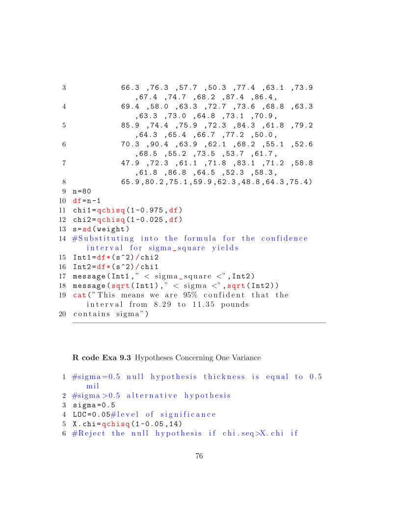
17 message(Int1 ,” < s igma _ s qua r e <”,Int2)18 message(sqrt(Int1),” < s igma <”,sqrt(Int2))19 cat(”This means we a r e 95% c o n f i d e n t tha t the
i n t e r v a l from 8 . 2 9 to 11 . 3 5 pounds20 c o n t a i n s s igma ”)
R code Exa 9.3 Hypotheses Concerning One Variance
1 #sigma=0.5 n u l l h yp o t h e s i s t h i c k n e s s i s e qua l to 0 . 5mi l
2 #sigma >0.5 a l t e r n a t i v e h yp o t h e s i s3 sigma =0.5
4 LOC =0.05#l e v e l o f s i g n i f i c a n c e5 X.chi=qchisq (1 -0.05 ,14)
6 #Re j e c t the n u l l h yp o t h e s i s i f c h i . seq>X. ch i i f
76
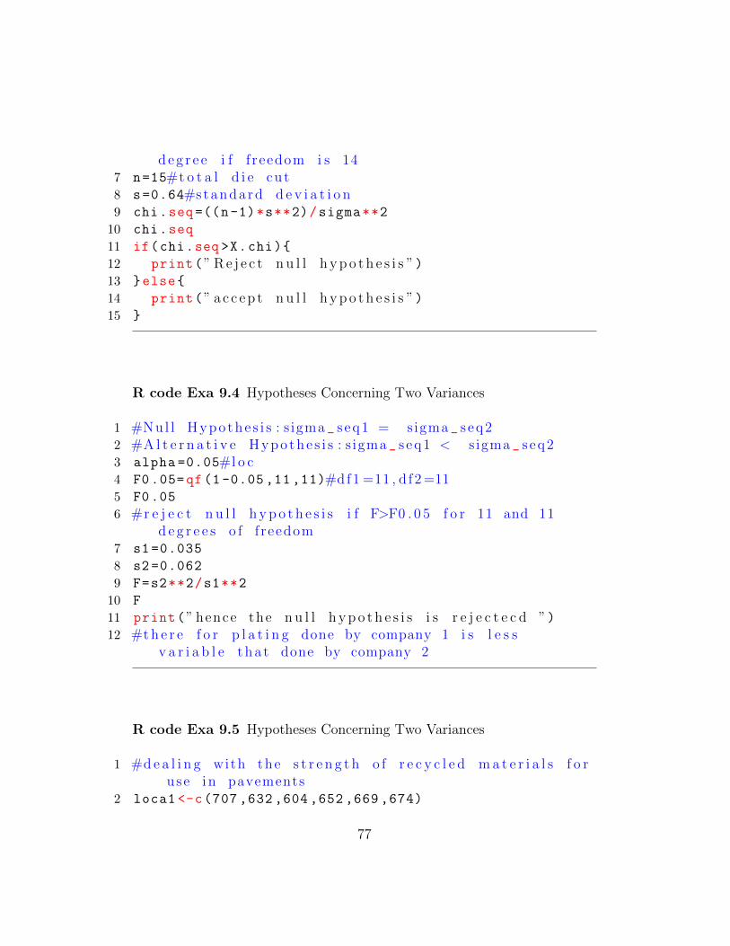
deg r e e i f f reedom i s 147 n=15#t o t a l d i e cut8 s=0.64#standard d e v i a t i o n9 chi.seq=((n-1)*s**2)/sigma**2
10 chi.seq
11 if(chi.seq >X.chi){
12 print(” Re j e c t n u l l h yp o t h e s i s ”)13 }else{
14 print(” a c c ep t n u l l h yp o t h e s i s ”)15 }
R code Exa 9.4 Hypotheses Concerning Two Variances
1 #Nul l Hypo the s i s : s igma _ s eq1 = sigma _ s eq22 #A l t e r n a t i v e Hypo the s i s : s igma _ s eq1 < s igma _ s eq23 alpha =0.05#l o c4 F0.05=qf(1 -0.05 ,11 ,11)#df1 =11 , d f2=115 F0.05
6 #r e j e c t n u l l h yp o t h e s i s i f F>F0 . 0 5 f o r 11 and 11d e g r e e s o f f reedom
7 s1 =0.035
8 s2 =0.062
9 F=s2**2/s1**2
10 F
11 print(” hence the n u l l h yp o t h e s i s i s r e j e c t e c d ”)12 #th e r e f o r p l a t i n g done by company 1 i s l e s s
v a r i a b l e tha t done by company 2
R code Exa 9.5 Hypotheses Concerning Two Variances
1 #de a l i n g with the s t r e n g t h o f r e c y c l e d ma t e r i a l s f o ruse i n pavements
2 loca1 <-c(707 ,632 ,604 ,652 ,669 ,674)
77
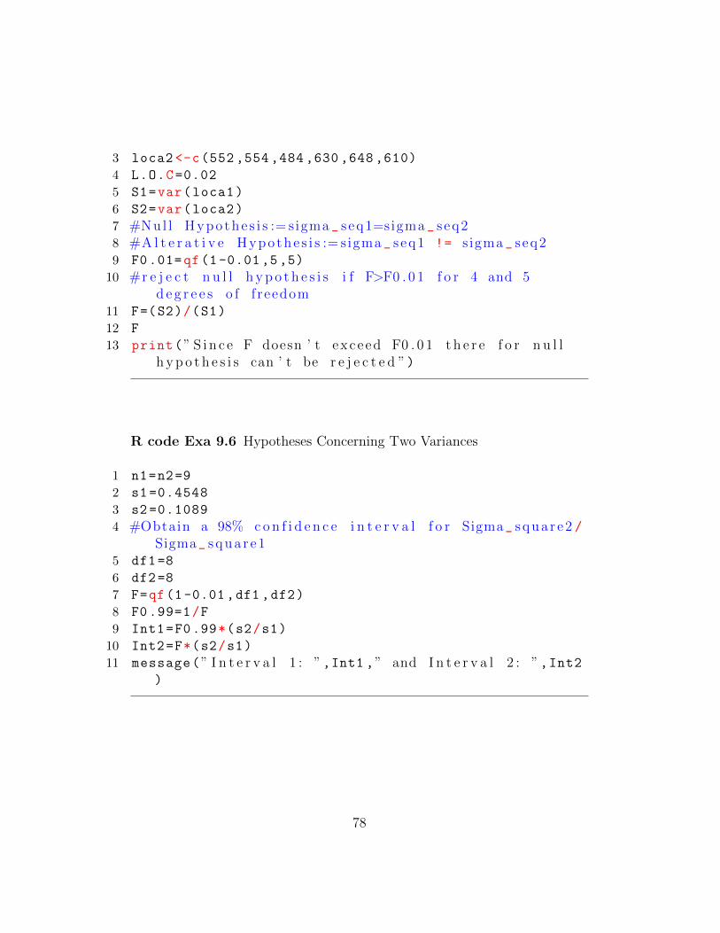
3 loca2 <-c(552 ,554 ,484 ,630 ,648 ,610)
4 L.O.C=0.02
5 S1=var(loca1)
6 S2=var(loca2)
7 #Nul l Hypo the s i s := sigma _ s eq1=sigma _ s eq28 #A l t e r a t i v e Hypo the s i s := sigma _ s eq1 != s igma _ s eq29 F0.01=qf(1-0.01,5,5)
10 #r e j e c t n u l l h yp o t h e s i s i f F>F0 . 0 1 f o r 4 and 5d e g r e e s o f f reedom
11 F=(S2)/(S1)
12 F
13 print(” S i n c e F doesn ’ t exceed F0 . 0 1 t h e r e f o r n u l lh yp o t h e s i s can ’ t be r e j e c t e d ”)
R code Exa 9.6 Hypotheses Concerning Two Variances
1 n1=n2=9
2 s1 =0.4548
3 s2 =0.1089
4 #Obtain a 98% c on f i d e n c e i n t e r v a l f o r Sigma_ squa r e2 /Sigma_ squa r e1
5 df1=8
6 df2=8
7 F=qf(1-0.01,df1 ,df2)
8 F0.99=1/F
9 Int1=F0.99*(s2/s1)
10 Int2=F*(s2/s1)
11 message(” I n t e r v a l 1 : ”,Int1 ,” and I n t e r v a l 2 : ”,Int2)
78
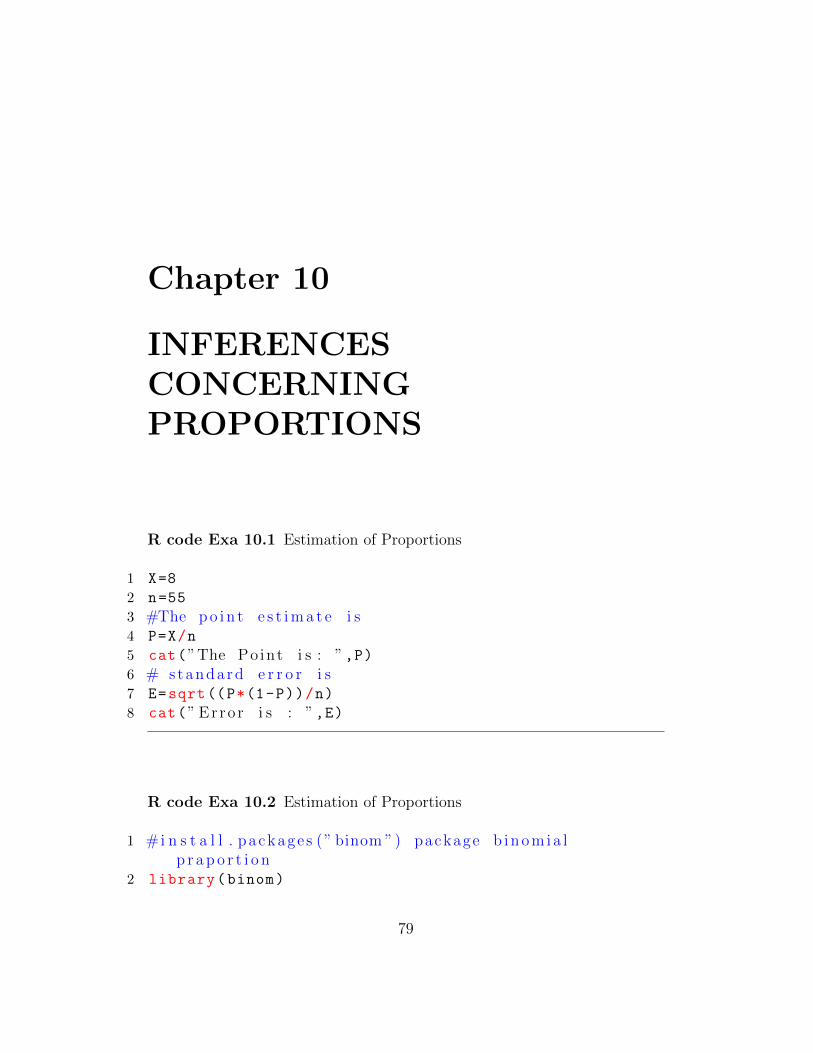
Chapter 10
INFERENCESCONCERNINGPROPORTIONS
R code Exa 10.1 Estimation of Proportions
1 X=8
2 n=55
3 #The po i n t e s t ima t e i s4 P=X/n
5 cat(”The Po int i s : ”,P)6 # standard e r r o r i s7 E=sqrt((P*(1-P))/n)
8 cat(” Er ro r i s : ”,E)
R code Exa 10.2 Estimation of Proportions
1 #i n s t a l l . package s (” binom ”) package b inom ia lp r a p o r t i o n
2 library(binom)
79
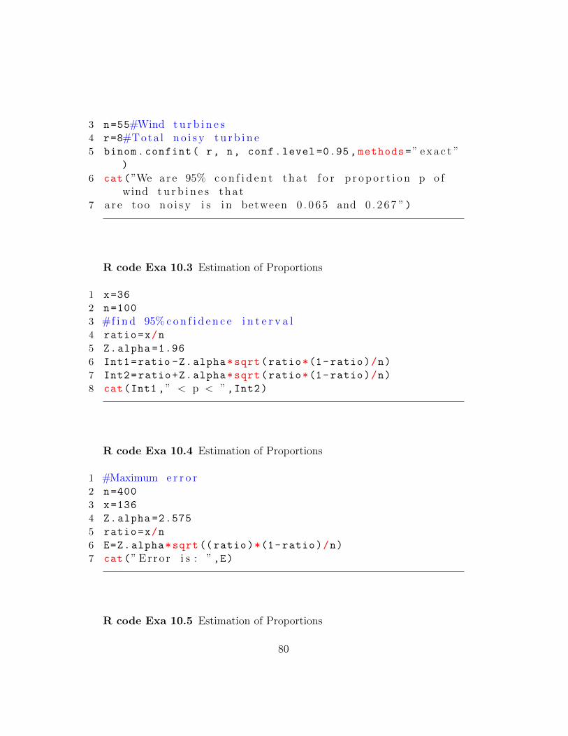
3 n=55#Wind t u r b i n e s4 r=8#Tota l n o i s y t u r b i n e5 binom.confint( r, n, conf.level =0.95, methods=” exac t ”
)
6 cat(”We ar e 95% c o n f i d e n t tha t f o r p r o p o r t i o n p o fwind t u r b i n e s tha t
7 a r e too no i s y i s i n between 0 . 0 6 5 and 0 . 2 67 ”)
R code Exa 10.3 Estimation of Proportions
1 x=36
2 n=100
3 #f i n d 95% c on f i d e n c e i n t e r v a l4 ratio=x/n
5 Z.alpha =1.96
6 Int1=ratio -Z.alpha*sqrt(ratio*(1-ratio)/n)
7 Int2=ratio+Z.alpha*sqrt(ratio*(1-ratio)/n)
8 cat(Int1 ,” < p < ”,Int2)
R code Exa 10.4 Estimation of Proportions
1 #Maximum e r r o r2 n=400
3 x=136
4 Z.alpha =2.575
5 ratio=x/n
6 E=Z.alpha*sqrt(( ratio)*(1-ratio)/n)
7 cat(” Er ro r i s : ”,E)
R code Exa 10.5 Estimation of Proportions
80
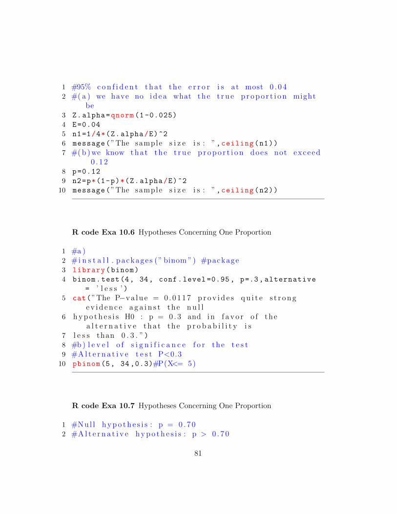
1 #95% c o n f i d e n t tha t the e r r o r i s at most 0 . 0 42 #( a ) we have no i d e a what the t r u e p r op o r t i o n might
be3 Z.alpha=qnorm (1 -0.025)
4 E=0.04
5 n1=1/4*(Z.alpha/E)^2
6 message(”The sample s i z e i s : ”,ceiling(n1))7 #(b )we know tha t the t r u e p r op o r t i o n does not exceed
0 . 1 28 p=0.12
9 n2=p*(1-p)*(Z.alpha/E)^2
10 message(”The sample s i z e i s : ”,ceiling(n2))
R code Exa 10.6 Hypotheses Concerning One Proportion
1 #a )2 #i n s t a l l . package s (” binom ”) #package3 library(binom)
4 binom.test(4, 34, conf.level =0.95, p=.3, alternative
= ’ l e s s ’ )5 cat(”The P−va lu e = 0 . 0117 p r o v i d e s q u i t e s t r o n g
e v i d en c e a g a i n s t the n u l l6 hypo t h e s i s H0 : p = 0 . 3 and in f a v o r o f the
a l t e r n a t i v e tha t the p r o b a b i l i t y i s7 l e s s than 0 . 3 . ”)8 #b) l e v e l o f s i g n i f i c a n c e f o r the t e s t9 #A l t e r n a t i v e t e s t P<0.3
10 pbinom(5, 34 ,0.3)#P(X<= 5)
R code Exa 10.7 Hypotheses Concerning One Proportion
1 #Nul l h yp o t h e s i s : p = 0 . 7 02 #A l t e r n a t i v e h yp o t h e s i s : p > 0 . 7 0
81
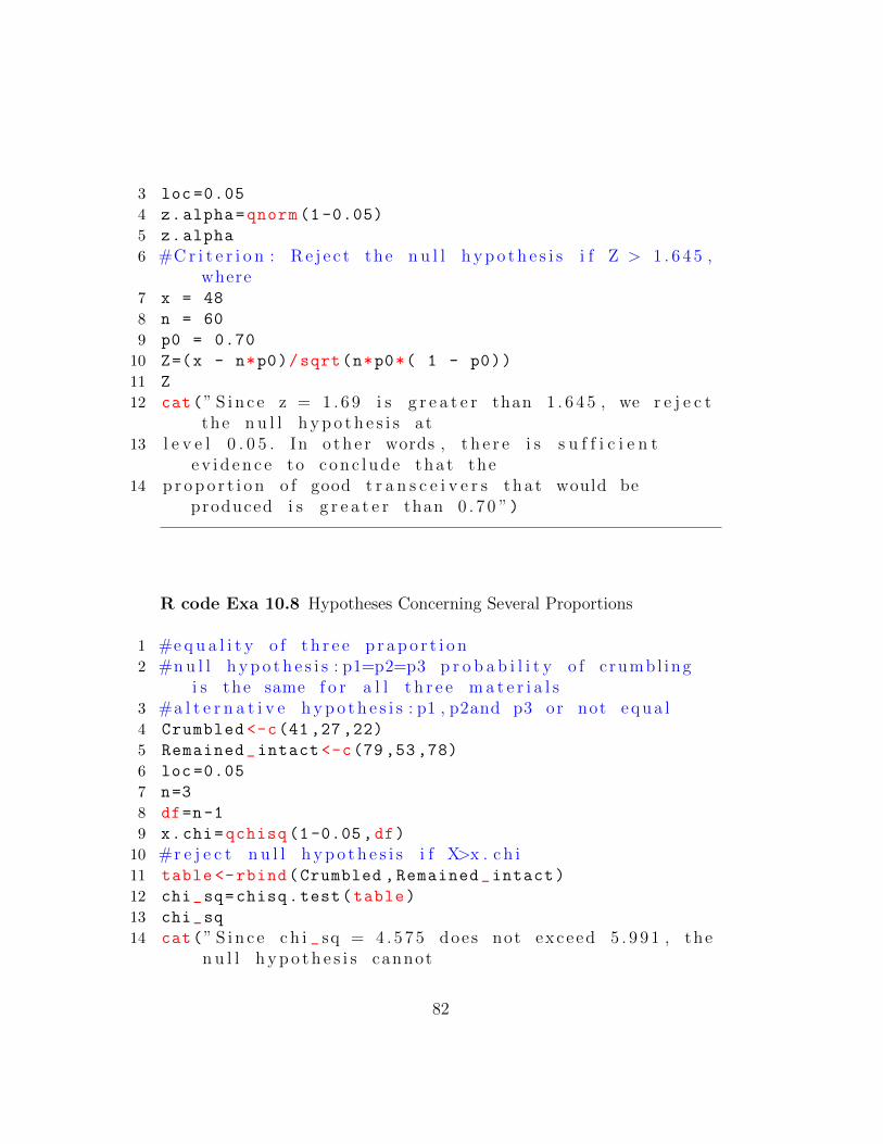
3 loc =0.05
4 z.alpha=qnorm (1 -0.05)
5 z.alpha
6 #Cr i t e r i o n : Re j e c t the n u l l h yp o t h e s i s i f Z > 1 . 6 4 5 ,where
7 x = 48
8 n = 60
9 p0 = 0.70
10 Z=(x - n*p0)/sqrt(n*p0*( 1 - p0))
11 Z
12 cat(” S i n c e z = 1 . 6 9 i s g r e a t e r than 1 . 6 4 5 , we r e j e c tthe n u l l h yp o t h e s i s at
13 l e v e l 0 . 0 5 . In o th e r words , t h e r e i s s u f f i c i e n te v i d en c e to conc l ude tha t the
14 p r op o r t i o n o f good t r a n s c e i v e r s tha t would beproduced i s g r e a t e r than 0 . 7 0 ”)
R code Exa 10.8 Hypotheses Concerning Several Proportions
1 #eq u a l i t y o f t h r e e p r ap o r t i o n2 #nu l l h yp o t h e s i s : p1=p2=p3 p r o b a b i l i t y o f c rumbl ing
i s the same f o r a l l t h r e e ma t e r i a l s3 #a l t e r n a t i v e h yp o t h e s i s : p1 , p2and p3 or not equa l4 Crumbled <-c(41 ,27 ,22)
5 Remained_intact <-c(79 ,53 ,78)
6 loc =0.05
7 n=3
8 df=n-1
9 x.chi=qchisq (1-0.05,df)
10 #r e j e c t n u l l h yp o t h e s i s i f X>x . c h i11 table <-rbind(Crumbled ,Remained_intact)
12 chi_sq=chisq.test(table)
13 chi_sq
14 cat(” S i n c e c h i _ sq = 4 . 5 75 does not exceed 5 . 9 9 1 , then u l l h yp o t h e s i s cannot
82
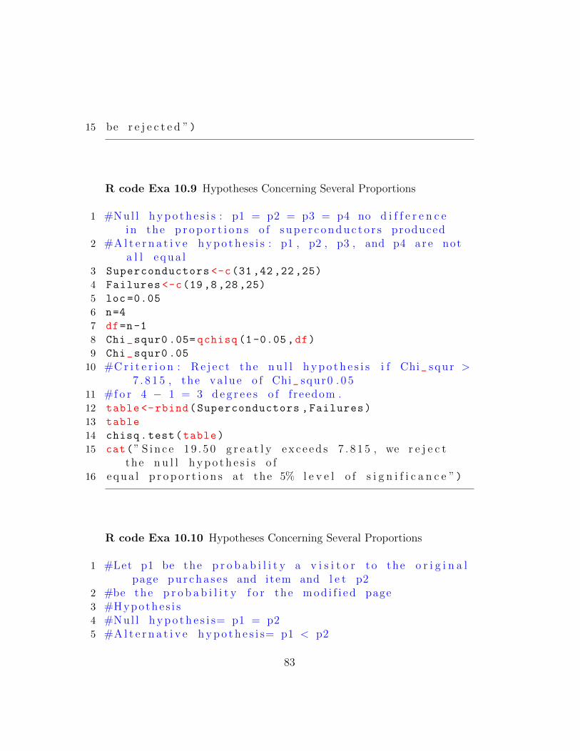
15 be r e j e c t e d ”)
R code Exa 10.9 Hypotheses Concerning Several Proportions
1 #Nul l h yp o t h e s i s : p1 = p2 = p3 = p4 no d i f f e r e n c ei n the p r o p o r t i o n s o f s up e r c ondu c t o r s produced
2 #A l t e r n a t i v e h yp o t h e s i s : p1 , p2 , p3 , and p4 a r e nota l l e qua l
3 Superconductors <-c(31 ,42 ,22 ,25)
4 Failures <-c(19,8,28 ,25)
5 loc =0.05
6 n=4
7 df=n-1
8 Chi_squr0 .05= qchisq (1-0.05,df)
9 Chi_squr0 .05
10 #Cr i t e r i o n : Re j e c t the n u l l h yp o t h e s i s i f Chi_ squr >7 . 8 1 5 , the va lu e o f Chi_ squr0 . 0 5
11 #f o r 4 − 1 = 3 d e g r e e s o f f reedom .12 table <-rbind(Superconductors ,Failures)
13 table
14 chisq.test(table)
15 cat(” S i n c e 19 . 5 0 g r e a t l y ex c e ed s 7 . 8 1 5 , we r e j e c tthe n u l l h yp o t h e s i s o f
16 equa l p r o p o r t i o n s at the 5% l e v e l o f s i g n i f i c a n c e ”)
R code Exa 10.10 Hypotheses Concerning Several Proportions
1 #Let p1 be the p r o b a b i l i t y a v i s i t o r to the o r i g i n a lpage pu r cha s e s and item and l e t p2
2 #be the p r o b a b i l i t y f o r the mod i f i e d page3 #Hypothe s i s4 #Nul l h yp o t h e s i s= p1 = p25 #A l t e r n a t i v e h yp o t h e s i s= p1 < p2
83
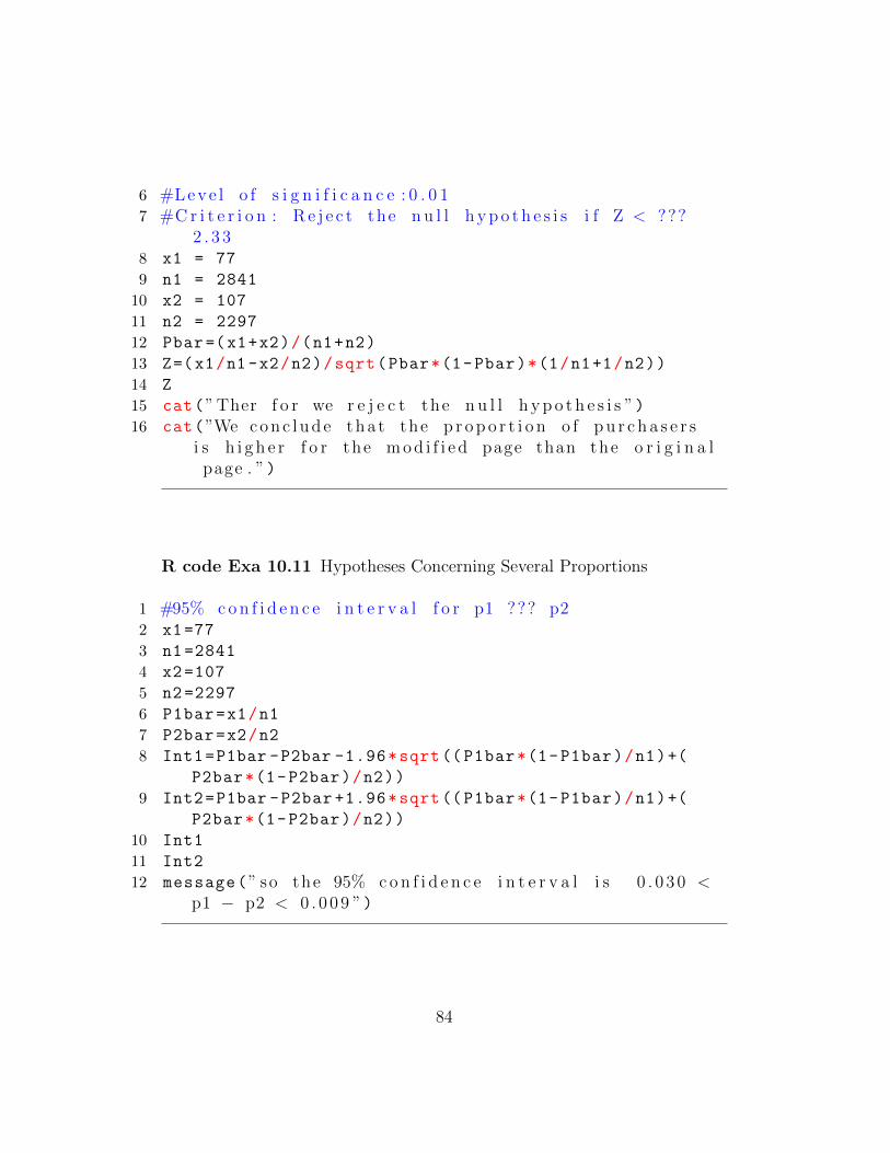
6 #Leve l o f s i g n i f i c a n c e : 0 . 0 17 #Cr i t e r i o n : Re j e c t the n u l l h yp o t h e s i s i f Z < ???
2 . 3 38 x1 = 77
9 n1 = 2841
10 x2 = 107
11 n2 = 2297
12 Pbar=(x1+x2)/(n1+n2)
13 Z=(x1/n1-x2/n2)/sqrt(Pbar*(1-Pbar)*(1/n1+1/n2))
14 Z
15 cat(”Ther f o r we r e j e c t the n u l l h yp o t h e s i s ”)16 cat(”We conc lude tha t the p r op o r t i o n o f pu r c h a s e r s
i s h i g h e r f o r the mod i f i e d page than the o r i g i n a lpage . ”)
R code Exa 10.11 Hypotheses Concerning Several Proportions
1 #95% con f i d e n c e i n t e r v a l f o r p1 ??? p22 x1=77
3 n1=2841
4 x2=107
5 n2=2297
6 P1bar=x1/n1
7 P2bar=x2/n2
8 Int1=P1bar -P2bar -1.96*sqrt(( P1bar*(1-P1bar)/n1)+(
P2bar*(1-P2bar)/n2))
9 Int2=P1bar -P2bar +1.96*sqrt(( P1bar*(1-P1bar)/n1)+(
P2bar*(1-P2bar)/n2))
10 Int1
11 Int2
12 message(” so the 95% c on f i d e n c e i n t e r v a l i s 0 . 0 3 0 <p1 − p2 < 0 . 0 09 ”)
84
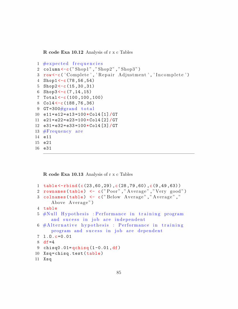
R code Exa 10.12 Analysis of r x c Tables
1 #expec t ed f r e q u e n c i e s2 column <-c(”Shop1”,”Shop2”,”Shop3”)3 row <-c( ’ Complete ’ , ’ Repa i r Adjustment ’ , ’ I n comp l e t e ’ )4 Shop1 <-c(78 ,56 ,54)
5 Shop2 <-c(15 ,30 ,31)
6 Shop3 <-c(7,14,15)
7 Total <-c(100 ,100 ,100)
8 Col4 <-c(188 ,76 ,36)
9 GT=300#grand t o t a l10 e11=e12=e13 =100*Col4 [1]/GT
11 e21=e22=e23 =100*Col4 [2]/GT
12 e31=e32=e33 =100*Col4 [3]/GT
13 #Frequency a r e14 e11
15 e21
16 e31
R code Exa 10.13 Analysis of r x c Tables
1 table <-rbind(c(23 ,60 ,29),c(28 ,79 ,60),c(9,49,63))
2 rownames(table) <- c(”Poor ”,”Average ”,”Very good ”)3 colnames(table) <- c(”Below Average ”,”Average ”,”
Above Average ”)4 table
5 #Nul l Hypo the s i s : Per formance i n t r a i n i n g programand s u c e s s i n j ob a r e independent
6 #A l t e r n a t i v e h yp o t h e s i s : Per formance i n t r a i n i n gprogram and s u c e s s i n j ob a r e dependent
7 l.O.c=0.01
8 df=4
9 chisq0 .01= qchisq (1-0.01,df)
10 Xsq=chisq.test(table)
11 Xsq
85
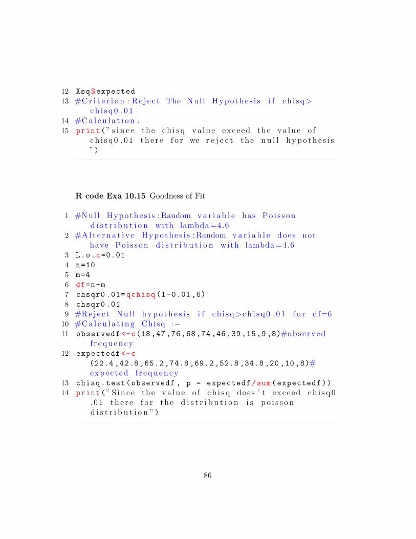
12 Xsq$expected
13 #Cr i t e r i o n : Re j e c t The Nu l l Hypo the s i s i f ch i s q>c h i s q 0 . 0 1
14 #Ca l c u l a t i o n :15 print(” s i n c e the c h i s q va l u e exceed the va lu e o f
c h i s q 0 . 0 1 t h e r e f o r we r e j e c t the n u l l h yp o t h e s i s”)
R code Exa 10.15 Goodness of Fit
1 #Nul l Hypo the s i s : Random v a r i a b l e has Po i s s ond i s t r i b u t i o n with lambda=4.6
2 #A l t e r n a t i v e Hypo the s i s : Random v a r i a b l e does nothave Po i s s on d i s t r i b u t i o n with lambda=4.6
3 L.o.c=0.01
4 n=10
5 m=4
6 df=n-m
7 chsqr0 .01= qchisq (1 -0.01 ,6)
8 chsqr0 .01
9 #Re j e c t Nu l l h yp o t h e s i s i f ch i sq>c h i s q 0 . 0 1 f o r d f=610 #Ca l c u l a t i n g Chisq :−11 observedf <-c(18,47,76,68,74,46,39,15,9,8)#obse rved
f r e qu en cy12 expectedf <-c
(22.4 ,42.8 ,65.2 ,74.8 ,69.2 ,52.8 ,34.8 ,20 ,10 ,8)#expec t ed f r e qu en cy
13 chisq.test(observedf , p = expectedf/sum(expectedf))
14 print(” S i n c e the va lu e o f c h i s q does ’ t exceed ch i s q 0. 0 1 t h e r e f o r the d i s t r i b u t i o n i s p o i s s o nd i s t r i b u t i o n ”)
86
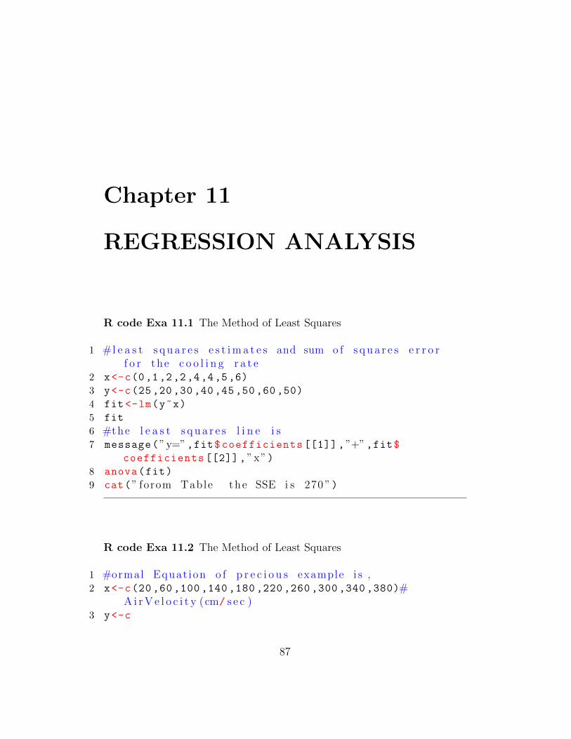
Chapter 11
REGRESSION ANALYSIS
R code Exa 11.1 The Method of Least Squares
1 #l e a s t s qua r e s e s t ima t e s and sum o f s qua r e s e r r o rf o r the c o o l i n g r a t e
2 x<-c(0,1,2,2,4,4,5,6)
3 y<-c(25 ,20 ,30 ,40 ,45 ,50 ,60 ,50)
4 fit <-lm(y~x)
5 fit
6 #the l e a s t s qua r e s l i n e i s7 message(”y=”,fit$coefficients [[1]],”+”,fit$
coefficients [[2]],”x”)8 anova(fit)
9 cat(” forom Table the SSE i s 270 ”)
R code Exa 11.2 The Method of Least Squares
1 #ormal Equat ion o f p r e c i o u s example i s ,2 x<-c(20 ,60 ,100 ,140 ,180 ,220 ,260 ,300 ,340 ,380)#
Ai rV e l o c i t y (cm/ s e c )3 y<-c
87
(0.18 ,0.37 ,0.35 ,0.78 ,0.56 ,0.75 ,1.18 ,1.36 ,1.17 ,1.650)
#Evaporat i on c o e f f i c e n t (mmˆ2/ s e c )4 table <-data.frame(x,y)
5 fit <-lm(y~x)
6 plot(x,y)
7 abline(fit)
8 message(” r e g r e s s i o n equa t i on i s : ”,fit$coefficients[[2]], ’ x + ’ ,fit$coefficients [[1]])
9 summary(aov(y~x))
10 cat(” from t a b l e SSE i s 0 . 2 0238 ”)11 print(”For x = 190 , we p r e d i c t tha t the e v apo r a t i o n
c o e f f i c i e n t w i l l be ”)12 Y<-data.frame(predict(fit ,data.frame(x=c(190)),
interval = ” c o n f i d e n c e ”))13 Y$fit
R code Exa 11.3 The Method of Least Squares
1 n = 50
2 x = 88.34
3 y = 305.58
4 Sxx = 7239.22
5 Sxy = 17840.1
6 Syy = 66976.2
7 #( a ) Find the l e a s t s qua r e s l i n e f o r p r e d i c t i n gh e i g h t from width .
8 beta=Sxy/Sxx
9 alpha=y-beta*x
10 cat( ’ h e i g h t = ’ ,87.88, ’ + ’ ,2.464, ’ width ’ )11 #(b ) Find the l e a s t s qua r e s l i n e f o r p r e d i c t i n g
width from he i gh12 beta=Sxy/Syy
13 alpha =88.34 -0.2664*305.58
14 cat( ’ width = ’ ,6.944, ’ + ’ ,0.266, ’ h e i g h t ’ )15 #( c ) Make a s c a t t e r p l o t and show both l i n e s .
88
16 Width <-c(77 ,80 ,83 ,73 ,79 ,100 ,93 ,92 ,101 ,87 ,96 ,99 ,94)
17 Height <-c
(290 ,292 ,289 ,284 ,271 ,292 ,308 ,303 ,308 ,315 ,309 ,300 ,305)
18 plot(Width ,Height)
19 Height =87.88 + 2.464*Width
20 lines(Width , Height)
21 Height = -26.11 + 3.759*Width
22 lines(Width , Height)
R code Exa 11.5 Inferences Based on the Least Squares Estimators
1 velocity <-c(20 ,60 ,100 ,140 ,180 ,220 ,260 ,300 ,340 ,380)
2 Evaporation <-c
(0.18 ,0.37 ,0.35 ,0.78 ,0.56 ,0.75 ,1.18 ,1.36 ,1.17 ,1.65)
3 Dat <-data.frame(velocity ,Evaporation)
4 fit <-lm(Evaporation~velocity)
5 summary(lm(Evaporation~velocity), data = Dat)
6 print(” the 95% c o n f i d e n c e l i m i t s a r e ”)7 predict(fit ,data.frame(velocity=c(0.1009737)),
interval = ” c o n f i d e n c e ”,level = 0.95)
R code Exa 11.6 Inferences Based on the Least Squares Estimators
1 velocity <-c(20 ,60 ,100 ,140 ,180 ,220 ,260 ,300 ,340 ,380)
2 Evaporation <-c
(0.18 ,0.37 ,0.35 ,0.78 ,0.56 ,0.75 ,1.18 ,1.36 ,1.17 ,1.65)
3 #Nul l h yp o t h e s i s : be ta= 04 #A l t e r n a t i v e h yp o t h e s i s : be ta != 05 loc =0.05
6 t=qt(1 -0.025 ,8)
89
7 #Cr i t e r i o n : Re j e c t the n u l l h yp o t h e s i s i f t < −2.306or t > 2 . 3 0 6 , where 2 . 3 0 6
8 #i s the va lu e o f t0 . 0 2 59 betabar =0.003829
10 beta=0
11 Sxx =132000
12 Se =0.1591
13 t=(betabar -beta)*sqrt(Sxx)/Se
14 t
15 cat(” De c i s i o n : S i n c e t = 8 . 7 44 ex c e ed s 2 . 3 0 6 , then u l l h yp o t h e s i s must be r e j e c t e d ,
16 we conc lude tha t t h e r e i s a r e l a t i o n s h i p between a i rv e l o c i t y and the ave rage ”)
R code Exa 11.7 Inferences Based on the Least Squares Estimators
1 #Peak l oad2 y1<-c(8.6 ,8.9 ,9.1)
3 y2<-c(9.0 ,9.3 ,9.4)
4 y3<-c( 9.5 ,9.8 ,9.8)
5 y4<-c(10.2 ,10.2 ,10.3)
6 x<-c(0,3,6,12)#Pr e s t r a i n7 x=c(0,0,0,3,3,3,6,6,6,12,12,12)
8 y=c(y1,y2,y3,y4)
9 #a )10 summary(lm(y~x))
11 summary(aov(y~x))
12 plot(x,y)
13 message(” the P−va lu e f o r the one−s i d e d t e s t i s l e s sthan 0 . 0 000 when rounded
14 down . This i s ve ry s t r o n g e v i d en c e tha t p r e s t r e s s i n gr e s u l t s i n s t r o n g e r
15 ma t e r i a l . ”)16 #b)17 fit <-lm(y~x)
90
18 #The e s t ima t ed r e g r e s s i o n l i n e i s19 cat(”y = ”,fit$coefficients [[1]],” + ”,fit$
coefficients [[2]],”x”)20 x=1# pe r c en t p r e s t r a i n21 y=data.frame(predict(fit ,data.frame(x=c(1)),interval
= ” c o n f i d e n c e ”))22 message(y$fit ,” kN”)23 #The 95% c on f i d e n c e i n t e r v a l becomes24 y
25 message(”We ar e 95% c o n f i d e n t tha t mean s t r e n g t h i sbetween 8 . 860385 and 9 . 182154 kN f o r a l l
26 a l l o y s h e e t s tha t cou ld undergo a p r e s t r a i n o f 1p e r c en t ”)
27 #c ) Note :−This i s Part ( b ) o f T .B28 x=9# pe r c en t p r e s t r a i n29 y=data.frame(predict(fit ,data.frame(x=c(9)),interval
= ” c o n f i d e n c e ”))30 message(y$fit ,” kN”)31 #The 95% c on f i d e n c e i n t e r v a l becomes32 y
33 message(”We ar e 95% c o n f i d e n t tha t mean s t r e n g t h i sbetween 9 . 7 9 and 10 . 0 9 kN f o r a l l
34 a l l o y s h e e t s tha t cou ld undergo a p r e s t r a i n o f 9p e r c en t ”)
35
36 #d) Note :−This i s Part ( c ) o f T .B37 cat(” , t h e r e a r e no o u t l i e r s i n the r e s i d u a l s and
the assumpt ion o f38 normal e r r o r s appea r s r e a s o n ab l e . We can r e l y upon
the39 s t a t i s t i c a l c o n c l u s i o n s above ”)
R code Exa 11.8 Inferences Based on the Least Squares Estimators
1 #95% p r e d i c t i o n l i m i t
91
2 #from example 73 y=9.938
4 t0.025=qt(1 -0.025 ,11)
5 Se =0.180634
6 n=12
7 Sxx =236.250
8 x0=9
9 xbar =5.25
10 Int1=y-t0.025*Se*sqrt (1+1/n+((x0-xbar)/Sxx))
11 Int2=y+t0.025*Se*sqrt (1+1/n+((x0-xbar)/Sxx))
12 Int1
13 Int2
14 cat(”We ar e 95% c o n f i d e n t tha t the ob s e rv ed va lu e o fpeak l oad f o r t h i s new
15 s h e e t o f aluminum l i e s between 9 . 5 1 and 10 . 3 7 kN”)
R code Exa 11.9 Inferences Based on the Least Squares Estimators
1 x0 = 18
2 y1<-c(8.6 ,8.9 ,9.1)
3 y2<-c(9.0 ,9.3 ,9.4)
4 y3<-c( 9.5 ,9.8 ,9.8)
5 y4<-c(10.2 ,10.2 ,10.3)
6 x<-c(0,3,6,12)
7 y<-c(mean(y1),mean(y2),mean(y3),mean(y4))
8 predict(lm(y~x),data.frame(x=c(18)),interval = ”c o n f i d e n c e ”,level = 0.95)
9 cat(”We ar e 95% c o n f i d e n t tha t the ob s e rv ed va lu e o fpeak l oad f o r t h i s
10 new sh e e t o f aluminum l i e s between 10 . 4 3 and 11 . 5 1kN”)
R code Exa 11.10 Curvilinear Regression
92
1 x<-c(2,3,6,10,15,20)
2 y<-c(164.7 ,156.1 ,142.5 ,133.8 ,114.6 ,107.1)
3 #a ) p l o t o f l o gy vs x4 #the r e l a t i o n sh i p between l o gy and x i s
e x p o n e n e t i a l cu rve5 plot(x,log(y))
6 #b) Reg r e s s i o n Equat ion7 summary(lm(log(y)~ x))
8 fit=lm(log(y)~ x)
9 #l o g a r i t hm i c form i s :10 cat(” l o g ( y ) = ”,fit$coefficients [2], ’ x + ’ ,fit$
coefficients [1])
11 #expon e n t i a l form i s :12 cat(”y = ”,exp (5.1257) , ’ * e ˆ( ’ ,fit$coefficients [2], ’ )
’ )13 #c ) Using the l o g a r i t hm i c form which i s more
conven i en t , we p r e d i c t14 result <-predict(fit ,data.frame(x=c(5)),interval = ”
c o n f i d e n c e ”,level = 0.95)
15 result
R code Exa 11.11 Curvilinear Regression
1 x<-c(0,1,2,3,4,5,6,7,8)#Amount o f v a r n i s h a d d i t i v e (grams )
2 y<-c(12 ,10.5 ,10 ,8 ,7 ,8 ,7.5 ,8.5 ,9.0)#Drying Time3 #a ) S c a t t e r p l o t4 plot(x,y)
5 #b) F i t a second−deg r e e po lynomia l6 fit <-lm(y~x+I(x^2))
7 fit
8 #Polynomia l e q u e s t i o n i s9 cat(”y = ”,fit$coefficients [[1]],””,fit$coefficients
[[2]],”x + ”,fit$coefficients [[3]],”xˆ2 ”)10 summary(fit)
93
11 lines(smooth.spline(x,predict(fit)),col= ’ b l u e ’ ,lwd=3)
12 #c ) d ry ing t ime o f the v a r n i s h when 6 . 5 grams o f thea d d i t i v e i s b e ing used
13 predict(fit ,data.frame(x=c(6.5)),interval = ”c o n f i d e n c e ”)
R code Exa 11.12 Multiple Regression
1 y<-c
(41 ,49 ,69 ,65 ,40 ,50 ,58 ,57 ,31 ,36 ,44 ,57 ,19 ,31 ,33 ,43)
2 x1<-c(1,2,3,4,1,2,3,4,1,2,3,4,1,2,3,4)
3 x2<-c(5,5,5,5,10,10,10,10,15,15,15,15,20,20,20,20)
4 fit <-lm(y~x1+x2)
5 summary(fit)
6 anova(lm(y~x1+x2))
7 print(”The l e a s t s qua r e s r e g r e s s i o n p l ane i s ”)8 cat(”Y=”,fit$coefficients [[1]], ’+ ’ ,fit$coefficients
[[2]], ’ x ’ ,fit$coefficients [[3]], ’ x ˆ2 ’ )9 cat(”This e qua t i on e s t ima t e s tha t the ave rage number
o f t w i s t s r e q u i r e d to break a10 bar i n c r e a s e s by 7 . 7 8 i f the p e r c en t o f e l ement A i s
i n c r e a s e d by 1% and x211 r ema ins f i x e d . ”)12
13 #For x1=2.5 and x2=1214 data <-data.frame(predict(fit ,data.frame(x1=c(2.5) ,x2
=c(12)),interval =” c o n f i d e n c e ”))15 data$fit
R code Exa 11.14 Correlation
94
1 #Time taken by 10 mechine to a s s emb l e i n morning xand a f t e r n o on y
2 x<-c
(11.1 ,10.3 ,12.0 ,15.1 ,13.7 ,18.5 ,17.3 ,14.2 ,14.8 ,15.3)
3 y<-c
(10.9 ,14.2 ,13.8 ,21.5 ,13.2 ,21.1 ,16.4 ,19.3 ,17.4 ,19.0)
4 plot(x,y,xlim=c(0,20),ylim=c(0 ,25))
5 r=cor(x,y)
6 r
R code Exa 11.15 Correlation
1 influent <-c(250 ,290 ,270 ,100 ,300 ,410 ,110 ,130 ,1100)
2 effluent <-c(19 ,10 ,17 ,11 ,70 ,60 ,18 ,30 ,180)
3 #( a )make s c a t t e r p l o t4 plot(influent ,effluent)
5 #(b ) l o g s c a t t e r p l o t6 plot(log(influent),log(effluent))
7 #( c )8 r1=cor(influent ,effluent)
9 r1
10 r2=cor(( influent),log(effluent))
11 r2
12 #d)13 cat(” hence r i s not r e a l l y a pp r o p r i a t e f o r the
o r i g i n a l data ”)
R code Exa 11.17 Correlation
1 #Nul l h yp o t h e s i s=d e l t a=02 #A l t e r n a t i v e h yp o t h e s i s= d e l t a !=0
95
3 l.o.c=0.05
4 n=10
5 r=0.732
6 #r e j e c t n u l l h yp o t h e s i s i f Z>1.96 or z <- 1 . 9 67 #Z=sq r t ( n−1)*Zbar8 Zbar=1/2*(log ((1+r)/(1-r)))
9 z=sqrt(n-3)*Zbar
10 Zbar
11 z
12 print(”There f o r we r e j e c t the n u l l h yp o t h e s i s ”)
R code Exa 11.18 Correlation
1 #Cin f i d e n c e i n t e r v a l f o r d e l t a normal p opu l a t i o n2 r=0.70
3 n=30#number o f s tuden t4 z0 .025=1.96
5 Zbar=1/2*log ((1+r)/(1-r))
6 Zbar
7 Int1=Zbar -z0.025/sqrt(n)
8 Int2=Zbar+z0.025/sqrt(n)
9 message(” the i n t e r v a l i s : ”,Int1 ,” and ”,Int2)10 r1=(exp(1)^Int1 -exp (1)^-Int1)/(exp(1)^Int1+exp(1)^-
Int1)
11 r1
12 r2=(exp(1)^Int2 -exp (1)^-Int2)/(exp(1)^Int2+exp(1)^-
Int2)
13 r2
14 #th e r e f o r the 95% c on f i d e n c e i n t e r v a l i s15 message(r1,” < rho < ”,r2)
R code Exa 11.19 Multiple Linear Regression Matrix Notation
96
1 #Mu l t i p l e L in ea r Reg r a s s i o n2 sumx1 =40
3 sumx2 =200
4 sumx1squar =120
5 sumx2squar =3000
6 sumy =723
7 x1.y=1963
8 x2.y=8210
9 x1.x2=500
10 n=16
11 XbarX=matrix(c(n,sumx1 ,sumx2 ,sumx1 ,sumx1squar ,x1.x2 ,
sumx2 ,x1.x2,sumx2squar),ncol = 3,byrow = TRUE)
12 XbarX
13 Inverse=solve(XbarX)
14 Xbary=matrix(c(sumy ,x1.y,x2.y))
15 Xbary
16 b=Inverse%*%Xbary
17 print(”The l e a s t squa r e e s t ima t i o n i s ”)18 b
R code Exa 11.20 Multiple Linear Regression Matrix Notation
1 X<-matrix(c(0,1,2,3,4))
2 X
3 y<-matrix(c(8,9,4,3,1))
4 n=5
5 XbarX <-matrix(c(n,sum(X),sum(X),sum(X^2)),ncol = 2,
byrow = TRUE)
6 XbarX
7 Inverse=solve(XbarX)
8 Xbary <-matrix(c(sum(y),sum(X*y)))
9 Xbary
10 b=Inverse%*%Xbary
11 b
12 message(”The F i t t e d e q u e s t i o n i s : y = ”,b[1],””,b
97
[2],”x ”)13 XX=matrix(c(1,0,1,1,1,2,1,3,1,4),byrow =TRUE ,ncol
=2)
14 XX
15 ybar=XX%*%b
16 ybar
17 #So the v e c t o r o f r e s i d u a l s18 result=y-ybar
19 #The Re s i dua l sum o f s qua r e s i s20 result2=t(result)
21 data=result2%*%result
22 Ssquar=data/(n-1-1)
23 message(Ssquar)
R code Exa 11.21 Multiple Linear Regression Matrix Notation
1 #Ca l c u l a t e e s t ima t ed v a r i a n c e s var ( b0 ) and var ( b1 )2 #With r e f e r i n g to p r e v i o u s example3 Inverse=matrix(c(0.6 , -0.2 , -0.2 ,0.1),ncol =2,byrow =
TRUE)
4 Ssquar =2
5 var=Inverse*Ssquar
6 print(”The e s t ima t ed v a r i a n c e s i s ”)7 var
8 varb0=var[1,1]
9 varb1=var[2,2]
10 print(”The var ( b0 ) i s ”)11 varb0
12 print(”The var ( b1 ) i s ”)13 varb1
98
Chapter 12
ANALYSIS OF VARIANCE
R code Exa 12.1 Completely Randomized Designs
1 #H0=the l a b o r a t o r i e s o b t a i n i n g c o n s i s t e n t r e s u l t2 #t in−c o a t i n g we ight f o r 12 d i s c i n each l i b o r a t o r y
i s show as3 LabA <-c
(0.25 ,0.27 ,0.22 ,0.30 ,0.27 ,0.28 ,0.32 ,0.24 ,0.31 ,0.26 ,0.22 ,0.28)
#Laborato ry A Data o f Tin−Cot ing we ight4 LabB <-c
(0.18 ,0.28 ,0.21 ,0.23 ,0.25 ,0.20 ,0.27 ,0.19 ,0.24 ,0.22 ,0.29 ,0.16)
#Laborato ry B Data o f Tin−Cot ing we ight5 LabC <-c
(0.19 ,0.25 ,0.27 ,0.24 ,0.18 ,0.26 ,0.28 ,0.24 ,0.25 ,0.20 ,0.21 ,0.19)
#Laborato ry C Data o f Tin−Cot ing we ight6 LabD <-c
(0.23 ,0.30 ,0.28 ,0.28 ,0.24 ,0.34 ,0.20 ,0.18 ,0.24 ,0.28 ,0.22 ,0.21)
#Laborato ry d Data o f Tin−Cot ing we ight7 #Nul l h yp o t h e s i s : mu1 = mu2 = mu3 = mu4 #Data
produce dy 4 d i f f l a b o r a t o r y has same mean8 #A l t e r n a t i v e h yp o t h e s i s : The mu’ s a r e not a l l e qua l9 #mu=mean10 #alpha =0.0511 F0.05=qf(1 -0.05 ,3 ,44)
99
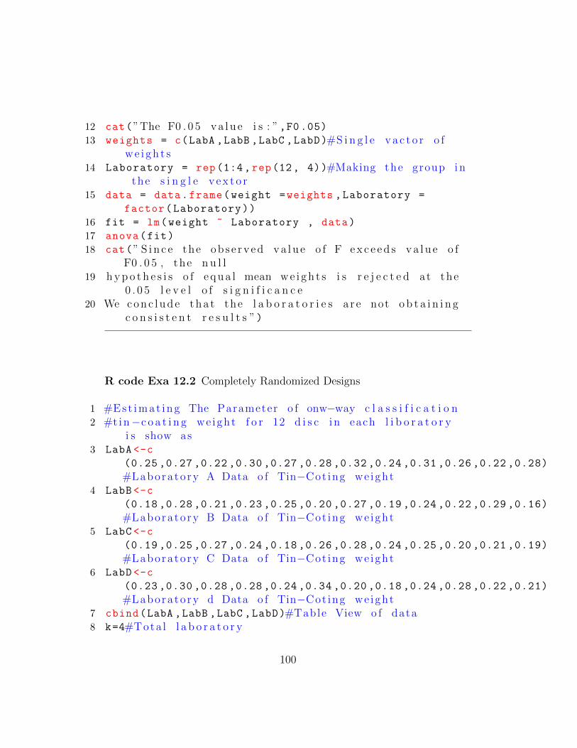
12 cat(”The F0 . 0 5 va lu e i s : ”,F0.05)13 weights = c(LabA ,LabB ,LabC ,LabD)#S i n g l e v a c t o r o f
we i gh t s14 Laboratory = rep(1:4,rep(12, 4))#Making the group in
the s i n g l e v ex t o r15 data = data.frame(weight =weights ,Laboratory =
factor(Laboratory))
16 fit = lm(weight ~ Laboratory , data)
17 anova(fit)
18 cat(” S i n c e the obs e rved va lu e o f F ex c e ed s va lu e o fF0 . 0 5 , the n u l l
19 hypo t h e s i s o f e qua l mean we i gh t s i s r e j e c t e d at the0 . 0 5 l e v e l o f s i g n i f i c a n c e
20 We conc lude tha t the l a b o r a t o r i e s a r e not o b t a i n i n gc o n s i s t e n t r e s u l t s ”)
R code Exa 12.2 Completely Randomized Designs
1 #Est imat ing The Parameter o f onw−way c l a s s i f i c a t i o n2 #t in−c o a t i n g we ight f o r 12 d i s c i n each l i b o r a t o r y
i s show as3 LabA <-c
(0.25 ,0.27 ,0.22 ,0.30 ,0.27 ,0.28 ,0.32 ,0.24 ,0.31 ,0.26 ,0.22 ,0.28)
#Laborato ry A Data o f Tin−Cot ing we ight4 LabB <-c
(0.18 ,0.28 ,0.21 ,0.23 ,0.25 ,0.20 ,0.27 ,0.19 ,0.24 ,0.22 ,0.29 ,0.16)
#Laborato ry B Data o f Tin−Cot ing we ight5 LabC <-c
(0.19 ,0.25 ,0.27 ,0.24 ,0.18 ,0.26 ,0.28 ,0.24 ,0.25 ,0.20 ,0.21 ,0.19)
#Laborato ry C Data o f Tin−Cot ing we ight6 LabD <-c
(0.23 ,0.30 ,0.28 ,0.28 ,0.24 ,0.34 ,0.20 ,0.18 ,0.24 ,0.28 ,0.22 ,0.21)
#Laborato ry d Data o f Tin−Cot ing we ight7 cbind(LabA ,LabB ,LabC ,LabD)#Table View o f data8 k=4#Tota l l a b o r a t o r y
100
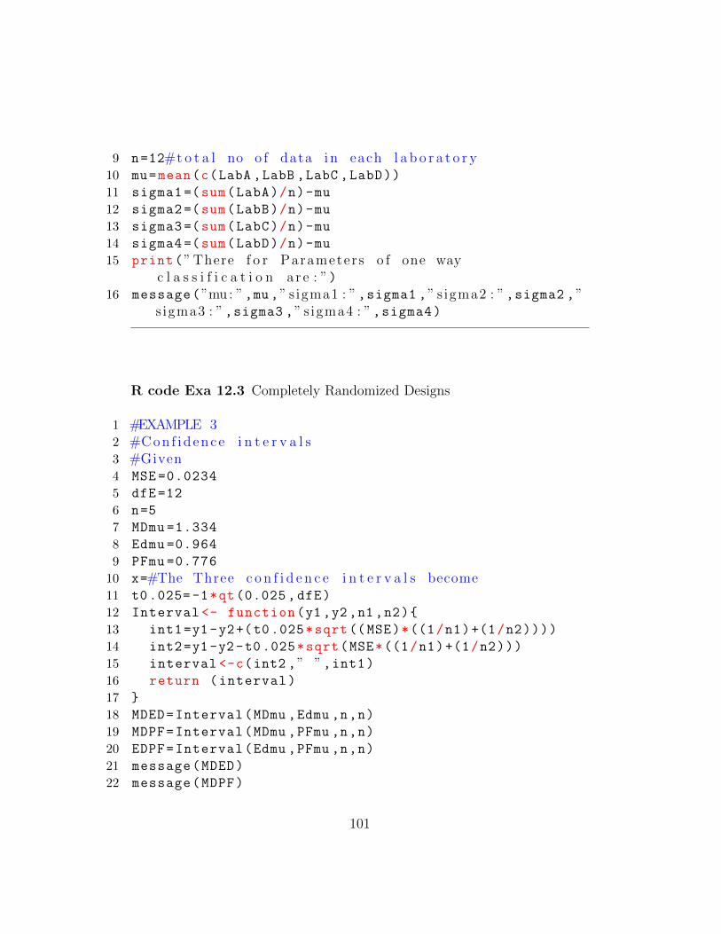
9 n=12#t o t a l no o f data i n each l a b o r a t o r y10 mu=mean(c(LabA ,LabB ,LabC ,LabD))
11 sigma1 =(sum(LabA)/n)-mu
12 sigma2 =(sum(LabB)/n)-mu
13 sigma3 =(sum(LabC)/n)-mu
14 sigma4 =(sum(LabD)/n)-mu
15 print(”There f o r Parameters o f one wayc l a s s i f i c a t i o n a r e : ”)
16 message(”mu : ”,mu ,” s igma1 : ”,sigma1 ,” s igma2 : ”,sigma2 ,”s igma3 : ”,sigma3 ,” s igma4 : ”,sigma4)
R code Exa 12.3 Completely Randomized Designs
1 #EXAMPLE 32 #Con f id ence i n t e r v a l s3 #Given4 MSE =0.0234
5 dfE =12
6 n=5
7 MDmu =1.334
8 Edmu =0.964
9 PFmu =0.776
10 x=#The Three c o n f i d e n c e i n t e r v a l s become11 t0.025= -1*qt(0.025 , dfE)
12 Interval <- function(y1,y2,n1,n2){
13 int1=y1-y2+(t0.025*sqrt((MSE)*((1/n1)+(1/n2))))
14 int2=y1-y2-t0.025*sqrt(MSE*((1/n1)+(1/n2)))
15 interval <-c(int2 ,” ”,int1)16 return (interval)
17 }
18 MDED=Interval(MDmu ,Edmu ,n,n)
19 MDPF=Interval(MDmu ,PFmu ,n,n)
20 EDPF=Interval(Edmu ,PFmu ,n,n)
21 message(MDED)
22 message(MDPF)
101
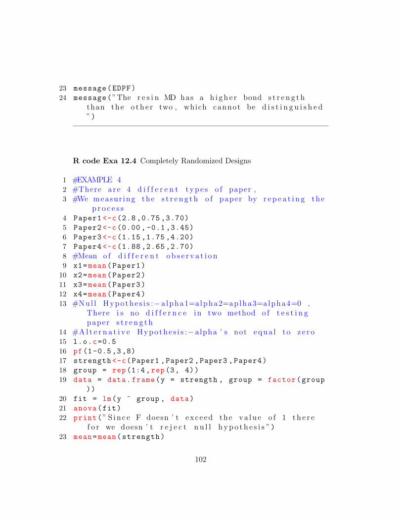
23 message(EDPF)
24 message(”The r e s i n MD has a h i g h e r bond s t r e n g t hthan the o th e r two , which cannot be d i s t i n g u i s h e d”)
R code Exa 12.4 Completely Randomized Designs
1 #EXAMPLE 42 #There a r e 4 d i f f e r e n t type s o f paper ,3 #We measur ing the s t r e n g t h o f paper by r e p e a t i n g the
p r o c e s s4 Paper1 <-c(2.8 ,0.75 ,3.70)
5 Paper2 <-c(0.00 , -0.1 ,3.45)
6 Paper3 <-c(1.15 ,1.75 ,4.20)
7 Paper4 <-c(1.88 ,2.65 ,2.70)
8 #Mean o f d i f f e r e n t o b s e r v a t i o n9 x1=mean(Paper1)
10 x2=mean(Paper2)
11 x3=mean(Paper3)
12 x4=mean(Paper4)
13 #Nul l Hypo the s i s :− a lpha1=a lpha2=ap lha3=a lpha4=0 ,There i s no d i f f e r n c e i n two method o f t e s t i n gpaper s t r e n g t h
14 #A l t e r n a t i v e Hypo the s i s :− alpha ’ s not equa l to z e r o15 l.o.c=0.5
16 pf(1-0.5,3,8)
17 strength <-c(Paper1 ,Paper2 ,Paper3 ,Paper4)
18 group = rep(1:4,rep(3, 4))
19 data = data.frame(y = strength , group = factor(group
))
20 fit = lm(y ~ group , data)
21 anova(fit)
22 print(” S i n c e F doesn ’ t exceed the va lu e o f 1 t h e r ef o r we doesn ’ t r e j e c t n u l l h yp o t h e s i s ”)
23 mean=mean(strength)
102
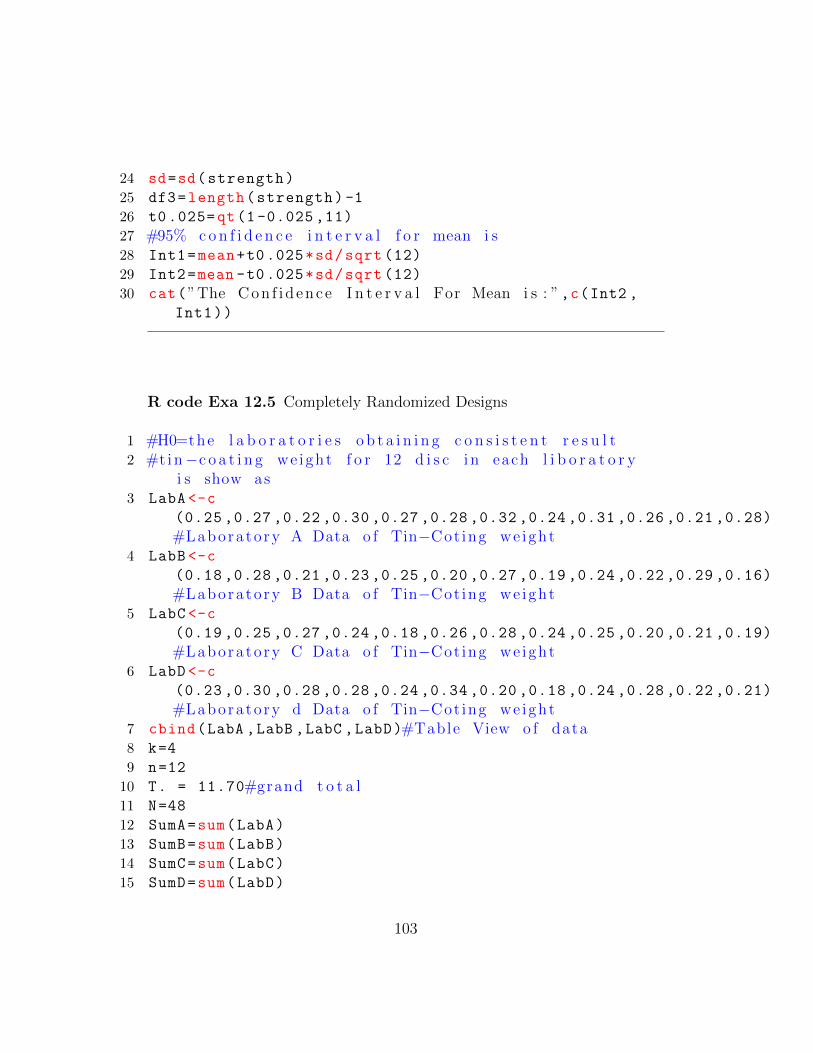
24 sd=sd(strength)
25 df3=length(strength) -1
26 t0.025=qt(1 -0.025 ,11)
27 #95% con f i d e n c e i n t e r v a l f o r mean i s28 Int1=mean+t0.025*sd/sqrt (12)
29 Int2=mean -t0.025*sd/sqrt (12)
30 cat(”The Con f i d ence I n t e r v a l For Mean i s : ”,c(Int2 ,Int1))
R code Exa 12.5 Completely Randomized Designs
1 #H0=the l a b o r a t o r i e s o b t a i n i n g c o n s i s t e n t r e s u l t2 #t in−c o a t i n g we ight f o r 12 d i s c i n each l i b o r a t o r y
i s show as3 LabA <-c
(0.25 ,0.27 ,0.22 ,0.30 ,0.27 ,0.28 ,0.32 ,0.24 ,0.31 ,0.26 ,0.21 ,0.28)
#Laborato ry A Data o f Tin−Cot ing we ight4 LabB <-c
(0.18 ,0.28 ,0.21 ,0.23 ,0.25 ,0.20 ,0.27 ,0.19 ,0.24 ,0.22 ,0.29 ,0.16)
#Laborato ry B Data o f Tin−Cot ing we ight5 LabC <-c
(0.19 ,0.25 ,0.27 ,0.24 ,0.18 ,0.26 ,0.28 ,0.24 ,0.25 ,0.20 ,0.21 ,0.19)
#Laborato ry C Data o f Tin−Cot ing we ight6 LabD <-c
(0.23 ,0.30 ,0.28 ,0.28 ,0.24 ,0.34 ,0.20 ,0.18 ,0.24 ,0.28 ,0.22 ,0.21)
#Laborato ry d Data o f Tin−Cot ing we ight7 cbind(LabA ,LabB ,LabC ,LabD)#Table View o f data8 k=4
9 n=12
10 T. = 11.70#grand t o t a l11 N=48
12 SumA=sum(LabA)
13 SumB=sum(LabB)
14 SumC=sum(LabC)
15 SumD=sum(LabD)
103
16 C=T.^2/N
17 SST=sum(LabA ^2)+sum(LabB ^2)+sum(LabC ^2)+sum(LabD ^2)-
C
18 SSTr =0.0135
19 SSE=SST -SSTr
20 MSTr=SSTr/(k-1)
21 MSE =0.0015
22 F=MSTr/MSE
23 F
R code Exa 12.6 Randomized Block Designs
1 Source <-c( ’ Treatments ’ , ’ B lock s ’ , ’ E r ro r ’ )2 Treatment1 <-c(13,8,9,6)
3 Treatment2 <-c(7,3,6,4)
4 Treatment3 <-c(13,7,12,8)
5 Temp <-c(Treatment1 ,Treatment2 ,Treatment3)
6 f = c(” Item1 ”, ” Item2 ”, ” Item3 ”, ” Item4 ”)7 k = 4 # number o f t r ea tment l e v e l s8 n = 3 # number o f c o n t r o l b l o c k s9 tm = gl(k, 1, n*k, factor(f)) # matching t r ea tment
10 tm
11 blk = gl(n, k, k*n) # b l o c k i n g f a c t o r12 blk
13 av = aov(Temp ~blk+ tm)
14 summary(av)
15 F0.05=qf(1-0.05,2,6)
16 cat(”The va lu e o f F0 . 0 5 with 2 and 6 d e g r e e s o ff reedom i s 5 . 1 4 , so we r e j e c t the n u l l
17 hypo t h e s i s o f e qua l mean p a r t i c u l a t e ma t e r i a lremoval . B l o ck ing was impor tant because
18 we a l s o r e j e c t the n u l l h yp o t h e s i s o f e qua lb l o ck means”)
104
R code Exa 12.7 Randomized Block Designs
1 #There a r e 4 d i f f e r e n t type o f D e t e r g e n t f o r engen .2 #There a r e 3 eng i n e3 #Nul l h yp o t h e s i s : a lpha1=a lpha2=apha3=0 and beta1=
beta2=beta3=04 #A l t e r n a t i v e h yp o t h e s i s : The a l pha s and be t a s not
equa l to z e r o5 l.o.c=0.01
6 #C r i t e r i a : For t r ea tment , r e j e c t n u l l h yp o t h e s i s i f F>9 .78 , the va lu e o f F0 . 0 1 with d f i s 3 and 6
7 #f o r b l o ck r e j e c t n u l l h yp o t h e s i s i f F>10.92 f o r 2and 6 d e g r e e s o f f reedom
8 #Ca l c u l a t i o n9 Detergent_A<-c(45 ,43 ,51)
10 Detergent_B<-c(47 ,46 ,52)
11 Detergent_C<-c(48 ,50 ,55)
12 Detergent_D<-c(42 ,37 ,49)
13 data <-c(Detergent_A,Detergent_B,Detergent_C,
Detergent_D)
14 f = c(” Item1 ”, ” Item2 ”, ” Item3 ”)15 k = 3 # number o f t r ea tment l e v e l s16 n = 4 # number o f c o n t r o l b l o c k s17 Engines= gl(k, 1, n*k, factor(f))# matching
t r ea tment18 Detergents= gl(n, k, k*n) # b l o c k i n g f a c t o r19 av = aov(data ~Detergents+ Engines)
20 summary(av)
21 print(” S i c e FDet exceed the va lu e 9 . 7 8 t h e r e weConclude tha t t h e r e i s d i f f e r e n c e i n e f f e c t i v n e s si n Det e rg en t ”)
22 print(” S i n c e FEn exceed the va l u e 10 . 9 2 t h e r e f o r weconc l ude tha t t h e r e i s d i f f e r e n c e i n r e s u l t
ob t a i n by 3 machine ”)
105
R code Exa 12.8 Randomized Block Designs
1 #Data from Example 72 Tem=c(45 ,43 ,51 ,47 ,46 ,52 ,48 ,50 ,55 ,42 ,37 ,49)
3 data <-matrix(c
(45 ,43 ,51 ,139 ,47 ,46 ,52 ,145 ,48 ,50 ,55 ,153 ,42 ,37 ,49 ,128 ,182 ,176 ,207 ,565)
,ncol=4,byrow=TRUE)
4 data
5 rownames(data)<-c(” Dete rg en t A”,” Dete rg en t B”,”Dete rg en t C”,” Dete rg en t D”,” To ta l s ”)
6 colnames(data)<-c(”Engine 1”,”Engine 2”,”Engine 3”,”To ta l s ”)
7 data
8 a = 4
9 b = 3
10 T1. = 139
11 T2. = 145
12 T3. = 153
13 T4. = 128
14 T.1 = 182
15 T.2 = 176
16 T.3 = 207
17 T.. = 565
18 Sumy =26867
19 n=12
20 C=T..^2/n#f a c t o r21 C
22 SST=sum(Tem^2)-C
23 SST
24 SSTr =((139^2+145^2+153^2+128^2)/3)-C
25 SSTr
26 SSB =((182^2+176^2+207^2)/4)-C
27 SSB
28 SSE=SST -SSTr -SSB
106
29 SSE
R code Exa 12.9 Multiple Comparisons
1 #Find 94% Bon f e r r o n i S imu l t aneou sCon f i d enc e i n t e r v a l2 MSE =0.0237
3 alpha =0.06
4 k=3
5 l.o.c=alpha/k*(k-1)
6 df=12
7 t0.01=qt(1-0.01,df=12)
8 t0.01
9 MDmu =1.334
10 Edmu =0.964
11 PFmu =0.776
12 n=5
13 Interval <- function(y1,y2,n1,n2){
14 int1=y1-y2+t0.01*sqrt(MSE*((1/n1)+(1/n2)))
15 int2=y1-y2-t0.01*sqrt(MSE*((1/n1)+(1/n2)))
16 interval <-c(int2 ,” ”,int1)17 return (interval)
18 }
19 MDED=Interval(MDmu ,Edmu ,n,n)
20 MDPF=Interval(MDmu ,PFmu ,n,n)
21 EDED=Interval(Edmu ,PFmu ,n,n)
22 #There f o r the i n t e r v a l a r e as23 message(MDED)
24 message(MDPF)
25 message(EDED)
R code Exa 12.10 Multiple Comparisons
1 #Find 94% Bon f e r r o n i S imu l t aneou sCon f i d enc e i n t e r v a l
107
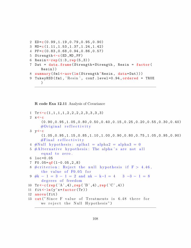
2 ED=c(0.99 ,1.19 ,0.79 ,0.95 ,0.90)
3 MD=c(1.11 ,1.53 ,1.37 ,1.24 ,1.42)
4 PF=c(0.83 ,0.68 ,0.94 ,0.86 ,0.57)
5 Strength <-c(ED ,MD,PF)
6 Resin <-rep(1:3,rep(5,3))
7 Dat = data.frame(Strength=Strength , Resin = factor(
Resin))
8 summary(fm1 <-aov(lm(Strength~Resin , data=Dat)))
9 TukeyHSD(fm1 , ’ Res in ’ , conf.level =0.94, ordered = TRUE
)
R code Exa 12.11 Analysis of Covariance
1 Tr<-c(1,1,1,1,2,2,2,2,3,3,3,3)
2 x<-c
(0.90 ,0.95 ,1.05 ,0.80 ,0.50 ,0.40 ,0.15 ,0.25 ,0.20 ,0.55 ,0.30 ,0.40)
#Or i g i n a l r e f l e c t i v i t y3 y<-c
(1.05 ,0.95 ,1.15 ,0.85 ,1.10 ,1.00 ,0.90 ,0.80 ,0.75 ,1.05 ,0.95 ,0.90)
#Fina l r e f l e c t i v i t y4 #Nul l h yp o t h e s i s : ap lha1 = a lpha2 = a lpha3 = 05 #A l t e r n a t i v e h yp o t h e s i s : The alpha ’ s a r e not a l l
e qua l to z e r o .6 loc =0.05
7 F0.05=qf(1-0.05,2,8)
8 #c r i t e r i o n : Re j e c t the n u l l h yp o t h e s i s i f F > 4 . 4 6 ,the va lu e o f F0 . 0 5 f o r
9 #k − 1 = 3 − 1 = 2 and nk − k−1 = 4 3 −3 − 1 = 8d e g r e e s o f f reedom
10 Tr<-c(rep( ’A ’ ,4),rep( ’B ’ ,4),rep( ’C ’ ,4))11 fit <-lm(y~x+factor(Tr))
12 anova(fit)
13 cat(” S i n c e F va lu e o f Treatments i s 6 . 4 8 t h e r e f o rwe r e j e c t the Nu l l Hypo the s i s ”)
108
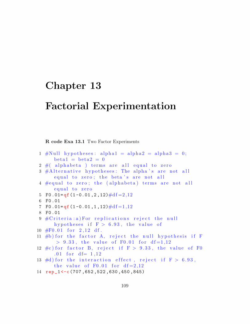
Chapter 13
Factorial Experimentation
R code Exa 13.1 Two Factor Experiments
1 #Nul l hypo the s e s : a lpha1 = a lpha2 = a lpha3 = 0 ;beta1 = beta2 = 0
2 #( a lphabe ta ) terms a r e a l l e qua l to z e r o3 #A l t e r n a t i v e hypo the s e s : The alpha ’ s a r e not a l l
e qua l to z e r o ; the beta ’ s a r e not a l l4 #equa l to z e r o ; the ( a l phabe ta ) terms a r e not a l l
e qua l to z e r o5 F0.01=qf(1 -0.01 ,2 ,12)#df =2 ,126 F0.01
7 F0.01=qf(1 -0.01 ,1 ,12)#df =1 ,128 F0.01
9 #C r i t e r i a : a ) For r e p l i c a t i o n s r e j e c t the n u l lhypo the s e s i f F > 6 . 9 3 , the va lu e o f
10 #F0 . 0 1 f o r 2 ,12 d f .11 #b) f o r the f a c t o r A, r e j e c t the n u l l h yp o t h e s i s i f F
> 9 . 3 3 , the va lu e o f F0 . 0 1 f o r d f =1 ,1212 #c ) f o r f a c t o r B, r e j e c t i f F > 9 . 3 3 , the va lu e o f F0
. 0 1 f o r d f= 1 ,1213 #d) f o r the i n t e r a c t i o n e f f e c t , r e j e c t i f F > 6 . 9 3 ,
the va lu e o f F0 . 0 1 f o r d f =2 ,1214 rep_1<-c(707 ,652 ,522 ,630 ,450 ,845)
109
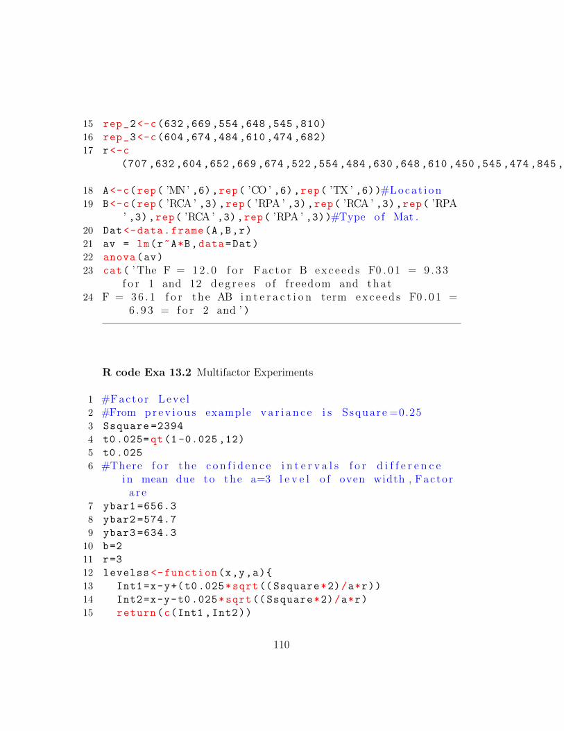
15 rep_2<-c(632 ,669 ,554 ,648 ,545 ,810)
16 rep_3<-c(604 ,674 ,484 ,610 ,474 ,682)
17 r<-c
(707 ,632 ,604 ,652 ,669 ,674 ,522 ,554 ,484 ,630 ,648 ,610 ,450 ,545 ,474 ,845 ,810 ,682)
18 A<-c(rep( ’MN’ ,6),rep( ’CO ’ ,6),rep( ’TX ’ ,6))#Loca t i on19 B<-c(rep( ’RCA ’ ,3),rep( ’RPA ’ ,3),rep( ’RCA ’ ,3),rep( ’RPA
’ ,3),rep( ’RCA ’ ,3),rep( ’RPA ’ ,3))#Type o f Mat .20 Dat <-data.frame(A,B,r)
21 av = lm(r~A*B,data=Dat)
22 anova(av)
23 cat( ’ The F = 12 . 0 f o r Facto r B ex c e ed s F0 . 0 1 = 9 . 3 3f o r 1 and 12 d e g r e e s o f f reedom and tha t
24 F = 36 . 1 f o r the AB i n t e r a c t i o n term exc e ed s F0 . 0 1 =6 . 9 3 = f o r 2 and ’ )
R code Exa 13.2 Multifactor Experiments
1 #Facto r Leve l2 #From p r e v i o u s example v a r i a n c e i s S square =0.253 Ssquare =2394
4 t0.025=qt(1 -0.025 ,12)
5 t0.025
6 #There f o r the c o n f i d e n c e i n t e r v a l s f o r d i f f e r e n c ei n mean due to the a=3 l e v e l o f oven width , Facto ra r e
7 ybar1 =656.3
8 ybar2 =574.7
9 ybar3 =634.3
10 b=2
11 r=3
12 levelss <-function(x,y,a){
13 Int1=x-y+(t0.025*sqrt(( Ssquare*2)/a*r))
14 Int2=x-y-t0.025*sqrt(( Ssquare*2)/a*r)
15 return(c(Int1 ,Int2))
110
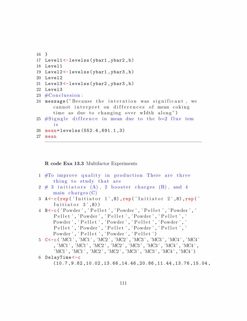
16 }
17 Level1 <-levelss(ybar1 ,ybar2 ,b)
18 Level1
19 Level2 <-levelss(ybar1 ,ybar3 ,b)
20 Level2
21 Level3 <-levelss(ybar2 ,ybar3 ,b)
22 Level3
23 #Conc lu e s i on :24 message(”Because the i n t e r a t i o n was s i g n i f i c a n t , we
cannot i n t e r p r e t on d i f f e r e n c e s o f mean cok ingt ime as due to chang ing ove r wIdth a l ong ”)
25 #S i g n g l e d i f f e e n c e i n mean due to the b=2 f l u e temi s
26 mean=levelss (552.4 ,691.1 ,3)
27 mean
R code Exa 13.3 Multifactor Experiments
1 #To improve q u a l i t y i n p r oduc t i on There a r e t h r e et h i ng to study tha t a r e
2 # 3 i n i t i a t o r s (A) , 2 b o o s t e r c ha r g e s (B) , and 4main cha r g e s (C)
3 A<-c(rep( ’ I n i t i a t o r 1 ’ ,8),rep( ’ I n i t i a t o r 2 ’ ,8),rep( ’I n i t i a t o r 3 ’ ,8))
4 B<-c( ’ Powder ’ , ’ P e l l e t ’ , ’ Powder ’ , ’ P e l l e t ’ , ’ Powder ’ , ’P e l l e t ’ , ’ Powder ’ , ’ P e l l e t ’ , ’ Powder ’ , ’ P e l l e t ’ , ’Powder ’ , ’ P e l l e t ’ , ’ Powder ’ , ’ P e l l e t ’ , ’ Powder ’ , ’P e l l e t ’ , ’ Powder ’ , ’ P e l l e t ’ , ’ Powder ’ , ’ P e l l e t ’ , ’Powder ’ , ’ P e l l e t ’ , ’ Powder ’ , ’ P e l l e t ’ )
5 C<-c( ’MC1 ’ , ’MC1 ’ , ’MC2 ’ , ’MC2 ’ , ’MC3 ’ , ’MC3 ’ , ’MC4 ’ , ’MC4 ’, ’MC1 ’ , ’MC1 ’ , ’MC2 ’ , ’MC2 ’ , ’MC3 ’ , ’MC3 ’ , ’MC4 ’ , ’MC4 ’ ,’MC1 ’ , ’MC1 ’ , ’MC2 ’ , ’MC2 ’ , ’MC3 ’ , ’MC3 ’ , ’MC4 ’ , ’MC4 ’ )
6 DelayTime <-c
(10.7 ,9.82 ,10.02 ,13.66 ,14.46 ,20.86 ,11.44 ,13.76 ,15.04 ,
111
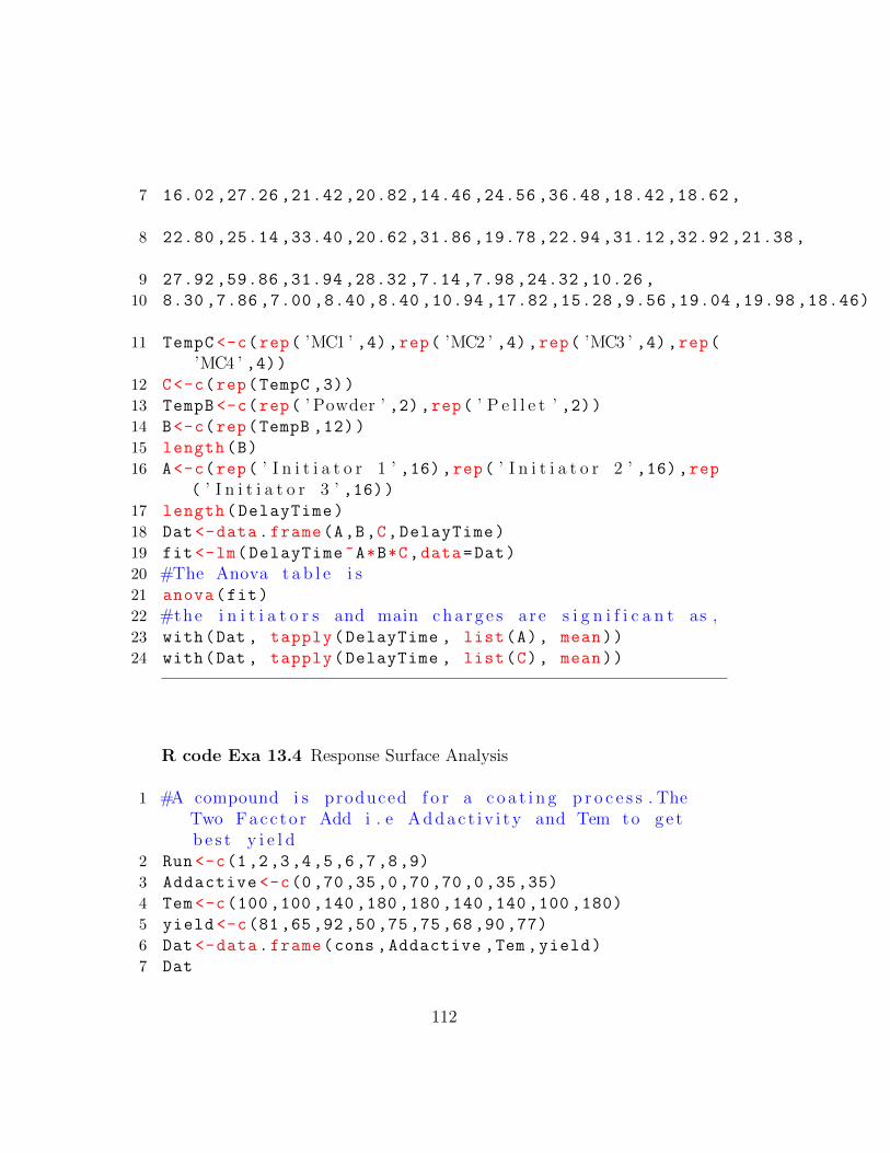
7 16.02 ,27.26 ,21.42 ,20.82 ,14.46 ,24.56 ,36.48 ,18.42 ,18.62 ,
8 22.80 ,25.14 ,33.40 ,20.62 ,31.86 ,19.78 ,22.94 ,31.12 ,32.92 ,21.38 ,
9 27.92 ,59.86 ,31.94 ,28.32 ,7.14 ,7.98 ,24.32 ,10.26 ,
10 8.30 ,7.86 ,7.00 ,8.40 ,8.40 ,10.94 ,17.82 ,15.28 ,9.56 ,19.04 ,19.98 ,18.46)
11 TempC <-c(rep( ’MC1 ’ ,4),rep( ’MC2 ’ ,4),rep( ’MC3 ’ ,4),rep(’MC4 ’ ,4))
12 C<-c(rep(TempC ,3))
13 TempB <-c(rep( ’ Powder ’ ,2),rep( ’ P e l l e t ’ ,2))14 B<-c(rep(TempB ,12))
15 length(B)
16 A<-c(rep( ’ I n i t i a t o r 1 ’ ,16),rep( ’ I n i t i a t o r 2 ’ ,16),rep( ’ I n i t i a t o r 3 ’ ,16))
17 length(DelayTime)
18 Dat <-data.frame(A,B,C,DelayTime)
19 fit <-lm(DelayTime~A*B*C,data=Dat)
20 #The Anova t a b l e i s21 anova(fit)
22 #the i n i t i a t o r s and main cha r g e s a r e s i g n i f i c a n t as ,23 with(Dat , tapply(DelayTime , list(A), mean))
24 with(Dat , tapply(DelayTime , list(C), mean))
R code Exa 13.4 Response Surface Analysis
1 #A compound i s produced f o r a c o a t i n g p r o c e s s . TheTwo Facc to r Add i . e Addac t i v i t y and Tem to ge tb e s t y i e l d
2 Run <-c(1,2,3,4,5,6,7,8,9)
3 Addactive <-c(0,70,35,0,70,70,0,35,35)
4 Tem <-c(100 ,100 ,140 ,180 ,180 ,140 ,140 ,100 ,180)
5 yield <-c(81 ,65 ,92 ,50 ,75 ,75 ,68 ,90 ,77)
6 Dat <-data.frame(cons ,Addactive ,Tem ,yield)
7 Dat
112
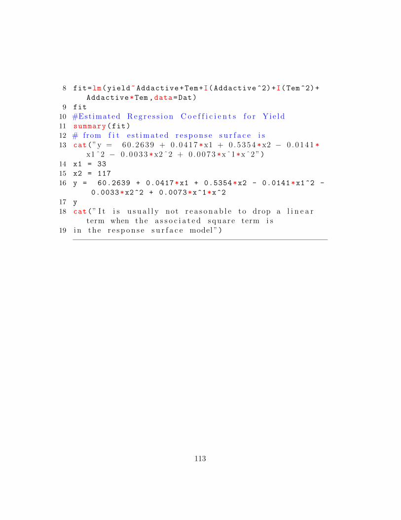
8 fit=lm(yield~Addactive+Tem+I(Addactive ^2)+I(Tem ^2)+
Addactive*Tem ,data=Dat)
9 fit
10 #Est imated Reg r e s s i o n C o e f f i c i e n t s f o r Y i e l d11 summary(fit)
12 # from f i t e s t ima t ed r e s p on s e s u r f a c e i s13 cat(”y = 60 . 2639 + 0 . 0417 *x1 + 0 . 5354 *x2 − 0 . 0 141 *
x1 ˆ2 − 0 . 0 033 *x2 ˆ2 + 0 . 0073 *xˆ1*xˆ2 ”)14 x1 = 33
15 x2 = 117
16 y = 60.2639 + 0.0417*x1 + 0.5354*x2 - 0.0141*x1^2 -
0.0033*x2^2 + 0.0073*x^1*x^2
17 y
18 cat(” I t i s u s u a l l y not r e a s o n a b l e to drop a l i n e a rterm when the a s s o c i a t e d squa r e term i s
19 i n the r e s p on s e s u r f a c e model ”)
113
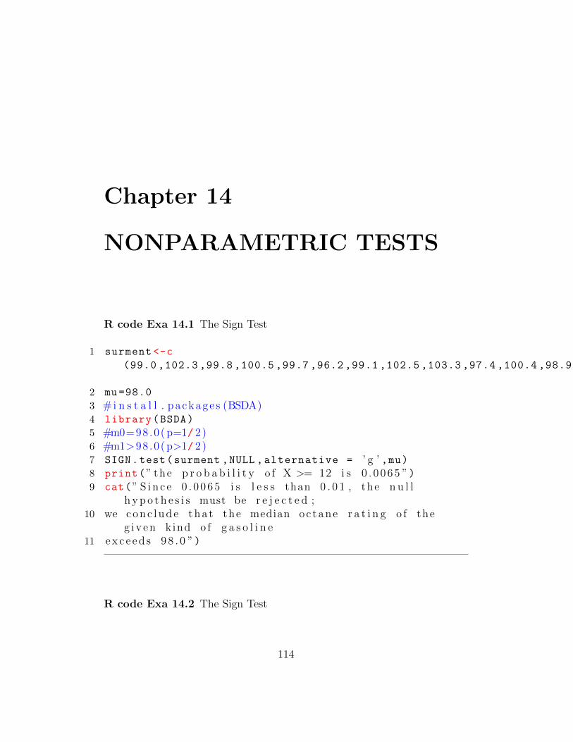
Chapter 14
NONPARAMETRIC TESTS
R code Exa 14.1 The Sign Test
1 surment <-c
(99.0 ,102.3 ,99.8 ,100.5 ,99.7 ,96.2 ,99.1 ,102.5 ,103.3 ,97.4 ,100.4 ,98.9 ,98.3 ,98.0 ,101.6)
2 mu=98.0
3 #i n s t a l l . package s (BSDA)4 library(BSDA)
5 #m0=98.0( p=1/ 2)6 #m1>98 .0(p>1/ 2)7 SIGN.test(surment ,NULL ,alternative = ’ g ’ ,mu)8 print(” the p r o b a b i l i t y o f X >= 12 i s 0 . 0 065 ”)9 cat(” S i n c e 0 . 0 065 i s l e s s than 0 . 0 1 , the n u l l
h yp o t h e s i s must be r e j e c t e d ;10 we conc lude tha t the median oc tane r a t i n g o f the
g i v en k ind o f g a s o l i n e11 ex c e ed s 9 8 . 0 ”)
R code Exa 14.2 The Sign Test
114
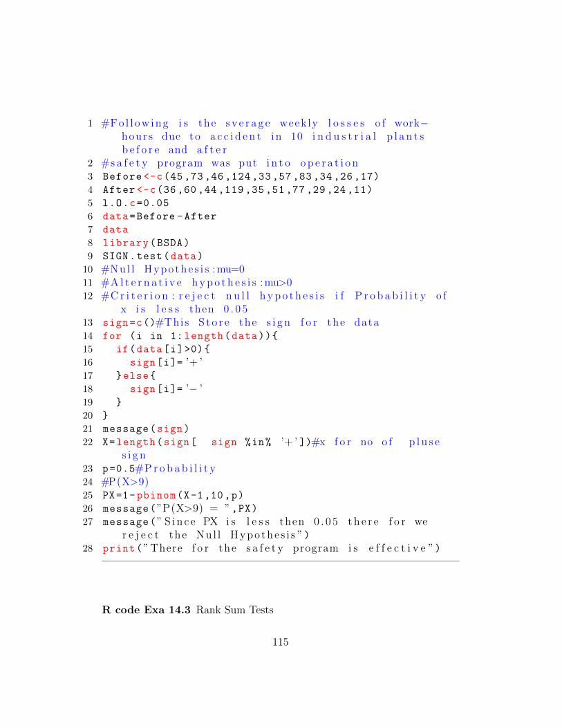
1 #Fo l l ow ing i s the s v e r a g e week ly l o s s e s o f work−hours due to a c c i d e n t i n 10 i n d u s t r i a l p l a n t sb e f o r e and a f t e r
2 #s a f e t y program was put i n t o o p e r a t i o n3 Before <-c(45 ,73 ,46 ,124 ,33 ,57 ,83 ,34 ,26 ,17)
4 After <-c(36 ,60 ,44 ,119 ,35 ,51 ,77 ,29 ,24 ,11)
5 l.O.c=0.05
6 data=Before -After
7 data
8 library(BSDA)
9 SIGN.test(data)
10 #Nul l Hypo the s i s :mu=011 #A l t e r n a t i v e h yp o t h e s i s :mu>012 #Cr i t e r i o n : r e j e c t n u l l h yp o t h e s i s i f P r o b a b i l i t y o f
x i s l e s s then 0 . 0 513 sign=c()#This S t o r e the s i g n f o r the data14 for (i in 1: length(data)){
15 if(data[i]>0){
16 sign[i]= ’+ ’17 }else{
18 sign[i]= ’− ’19 }
20 }
21 message(sign)
22 X=length(sign[ sign %in% ’+ ’ ])#x f o r no o f p l u s es i g n
23 p=0.5#Pr o b a b i l i t y24 #P(X>9)25 PX=1-pbinom(X-1,10,p)
26 message(”P(X>9) = ”,PX)27 message(” S i n c e PX i s l e s s then 0 . 0 5 t h e r e f o r we
r e j e c t the Nu l l Hypo the s i s ”)28 print(”There f o r the s a f e t y program i s e f f e c t i v e ”)
R code Exa 14.3 Rank Sum Tests
115
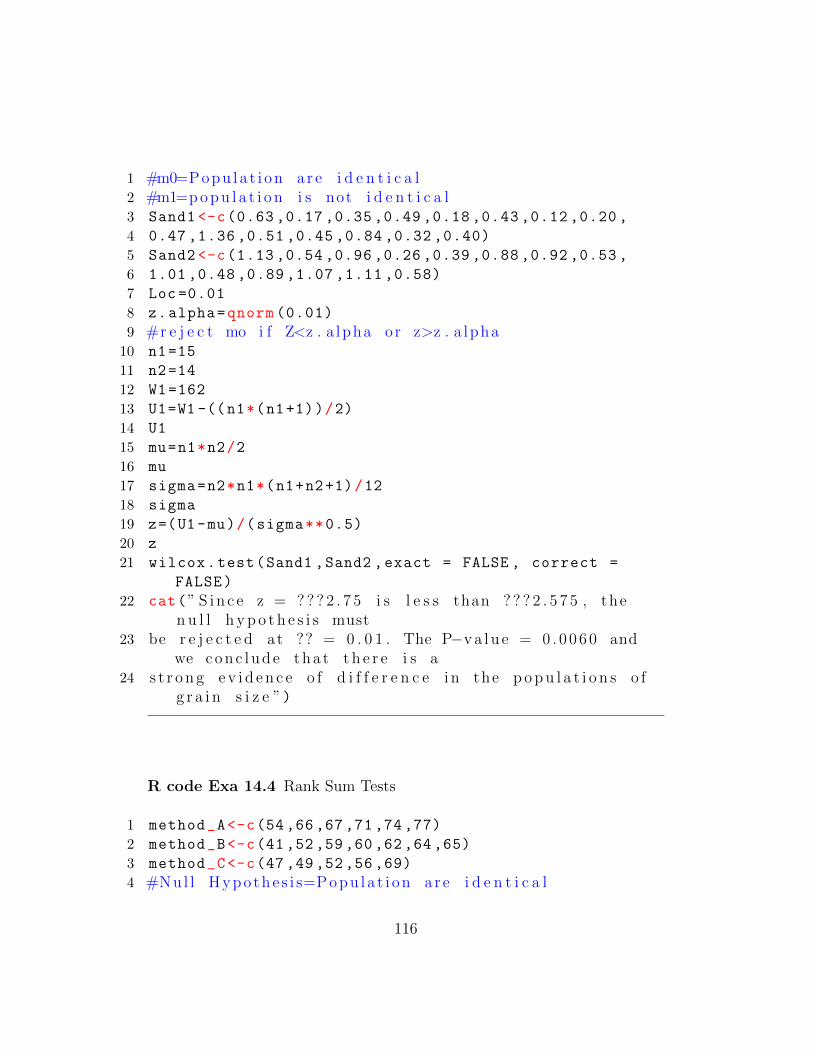
1 #m0=Popu la t i on a r e i d e n t i c a l2 #m1=popu l a t i o n i s not i d e n t i c a l3 Sand1 <-c(0.63 ,0.17 ,0.35 ,0.49 ,0.18 ,0.43 ,0.12 ,0.20 ,
4 0.47 ,1.36 ,0.51 ,0.45 ,0.84 ,0.32 ,0.40)
5 Sand2 <-c(1.13 ,0.54 ,0.96 ,0.26 ,0.39 ,0.88 ,0.92 ,0.53 ,
6 1.01 ,0.48 ,0.89 ,1.07 ,1.11 ,0.58)
7 Loc =0.01
8 z.alpha=qnorm (0.01)
9 #r e j e c t mo i f Z<z . a lpha or z>z . a lpha10 n1=15
11 n2=14
12 W1=162
13 U1=W1 -((n1*(n1+1))/2)
14 U1
15 mu=n1*n2/2
16 mu
17 sigma=n2*n1*(n1+n2+1)/12
18 sigma
19 z=(U1-mu)/(sigma**0.5)
20 z
21 wilcox.test(Sand1 ,Sand2 ,exact = FALSE , correct =
FALSE)
22 cat(” S i n c e z = ?? ? 2 . 7 5 i s l e s s than ? ? ? 2 . 5 7 5 , then u l l h yp o t h e s i s must
23 be r e j e c t e d at ?? = 0 . 0 1 . The P−va lu e = 0 . 0060 andwe conc lude tha t t h e r e i s a
24 s t r o n g e v i d en c e o f d i f f e r e n c e i n the p opu l a t i o n s o fg r a i n s i z e ”)
R code Exa 14.4 Rank Sum Tests
1 method_A<-c(54 ,66 ,67 ,71 ,74 ,77)
2 method_B<-c(41 ,52 ,59 ,60 ,62 ,64 ,65)
3 method_C<-c(47 ,49 ,52 ,56 ,69)
4 #Nul l Hypo the s i s=Popu la t i on a r e i d e n t i c a l
116
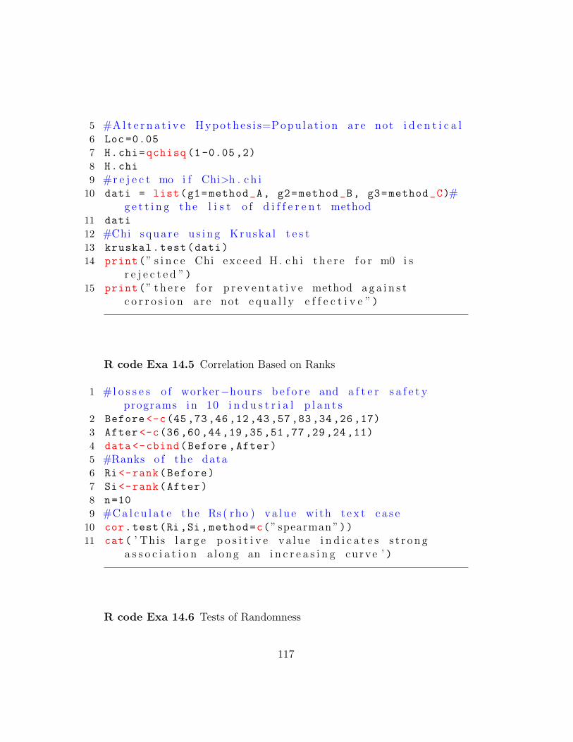
5 #A l t e r n a t i v e Hypo the s i s=Popu l a t i on a r e not i d e n t i c a l6 Loc =0.05
7 H.chi=qchisq (1 -0.05 ,2)
8 H.chi
9 #r e j e c t mo i f Chi>h . c h i10 dati = list(g1=method_A, g2=method_B, g3=method_C)#
g e t t i n g the l i s t o f d i f f e r e n t method11 dati
12 #Chi squa r e u s i n g Kruska l t e s t13 kruskal.test(dati)
14 print(” s i n c e Chi exceed H. c h i t h e r e f o r m0 i sr e j e c t e d ”)
15 print(” t h e r e f o r p r e v e n t a t i v e method a g a i n s tc o r r o s i o n a r e not e q u a l l y e f f e c t i v e ”)
R code Exa 14.5 Correlation Based on Ranks
1 #l o s s e s o f worker−hours b e f o r e and a f t e r s a f e t yprograms in 10 i n d u s t r i a l p l a n t s
2 Before <-c(45 ,73 ,46 ,12 ,43 ,57 ,83 ,34 ,26 ,17)
3 After <-c(36 ,60 ,44 ,19 ,35 ,51 ,77 ,29 ,24 ,11)
4 data <-cbind(Before ,After)
5 #Ranks o f the data6 Ri<-rank(Before)
7 Si<-rank(After)
8 n=10
9 #Ca l c u l a t e the Rs ( rho ) va l u e with t e x t c a s e10 cor.test(Ri,Si,method=c(” spearman ”))11 cat( ’ This l a r g e p o s i t i v e va lu e i n d i c a t e s s t r o n g
a s s o c i a t i o n a l ong an i n c r e a s i n g curve ’ )
R code Exa 14.6 Tests of Randomness
117
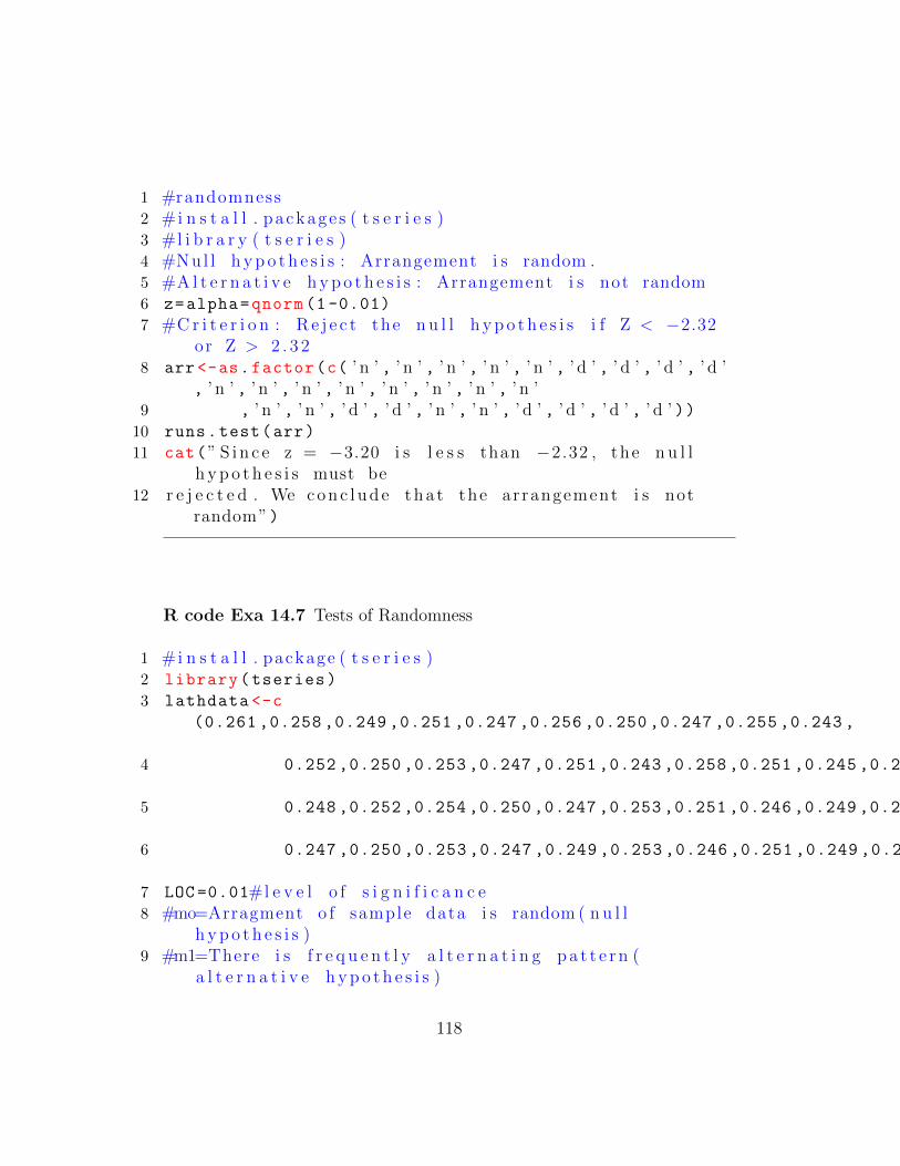
1 #randomness2 #i n s t a l l . package s ( t s e r i e s )3 #l i b r a r y ( t s e r i e s )4 #Nul l h yp o t h e s i s : Arrangement i s random .5 #A l t e r n a t i v e h yp o t h e s i s : Arrangement i s not random6 z=alpha=qnorm (1 -0.01)
7 #Cr i t e r i o n : Re j e c t the n u l l h yp o t h e s i s i f Z < −2.32or Z > 2 . 3 2
8 arr <-as.factor(c( ’ n ’ , ’ n ’ , ’ n ’ , ’ n ’ , ’ n ’ , ’ d ’ , ’ d ’ , ’ d ’ , ’ d ’, ’ n ’ , ’ n ’ , ’ n ’ , ’ n ’ , ’ n ’ , ’ n ’ , ’ n ’ , ’ n ’
9 , ’ n ’ , ’ n ’ , ’ d ’ , ’ d ’ , ’ n ’ , ’ n ’ , ’ d ’ , ’ d ’ , ’ d ’ , ’ d ’ ))10 runs.test(arr)
11 cat(” S i n c e z = −3.20 i s l e s s than −2.32 , the n u l lh yp o t h e s i s must be
12 r e j e c t e d . We conc l ude tha t the arrangement i s notrandom”)
R code Exa 14.7 Tests of Randomness
1 #i n s t a l l . package ( t s e r i e s )2 library(tseries)
3 lathdata <-c
(0.261 ,0.258 ,0.249 ,0.251 ,0.247 ,0.256 ,0.250 ,0.247 ,0.255 ,0.243 ,
4 0.252 ,0.250 ,0.253 ,0.247 ,0.251 ,0.243 ,0.258 ,0.251 ,0.245 ,0.250 ,
5 0.248 ,0.252 ,0.254 ,0.250 ,0.247 ,0.253 ,0.251 ,0.246 ,0.249 ,0.252 ,
6 0.247 ,0.250 ,0.253 ,0.247 ,0.249 ,0.253 ,0.246 ,0.251 ,0.249 ,0.253)
7 LOC =0.01#l e v e l o f s i g n i f i c a n c e8 #mo=Arragment o f sample data i s random ( n u l l
h yp o t h e s i s )9 #m1=There i s f r e q u e n t l y a l t e r n a t i n g pa t t e r n (
a l t e r n a t i v e h yp o t h e s i s )
118
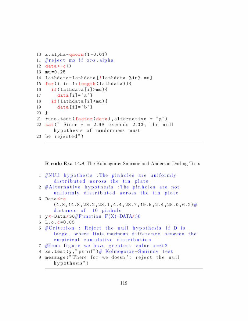
10 z.alpha=qnorm (1 -0.01)
11 #r e j e c t mo i f z>z . a lpha12 data <-c()
13 mu=0.25
14 lathdata=lathdata[!lathdata %in% mu]
15 for(i in 1: length(lathdata)){
16 if(lathdata[i]>mu){
17 data[i]= ’ a ’ }18 if(lathdata[i]<mu){
19 data[i]= ’ b ’ }20 }
21 runs.test(factor(data),alternative = ”g”)22 cat(” S i n c e z = 2 . 9 8 ex c e ed s 2 . 3 3 , the n u l l
h yp o t h e s i s o f randomness must23 be r e j e c t e d ”)
R code Exa 14.8 The Kolmogorov Smirnov and Anderson Darling Tests
1 #NUll h yp o t h e s i s : The p i n h o l e s a r e un i f o rm lyd i s t r i b u t e d a c r o s s the t i n p l a t e
2 #A l t e r n a t i v e h yp o t h e s i s : The p i n h o l e s a r e notun i f o rm ly d i s t r i b u t e d a c r o s s the t i n p l a t e
3 Data <-c
(4.8 ,14.8 ,28.2 ,23.1 ,4.4 ,28.7 ,19.5 ,2.4 ,25.0 ,6.2)#d i s t a n c e o f 10 p i n h o l e
4 y<-Data/30#Funct ion F(X)=DATA/305 L.o.c=0.05
6 #Cr i t e r i o n : Re j e c t the n u l l h yp o t h e s i s i f D i sl a r g e . where Dnis maximum d i f f e r e n c e between theemp i r i c a l cumu la t i v e d i s t r i b u t i o n
7 #From f i g u r e we have g r e a t e s t va l u e x=6.28 ks.test(y,” pun i f ”)# Kolmogorov−Smirnov t e s t9 message(”There f o r we doesn ’ t r e j e c t the n u l l
h yp o t h e s i s ”)
119
R code Exa 14.9 The Kolmogorov Smirnov and Anderson Darling Tests
1 #i n s t a l l . package s (” n o r t e s t ”)2 library(nortest)
3 #d i s t a n c e s i n i n c h e s o f 10 p i n h o l e s from one edge o fa l ong s t r i p
4 data <-c
(2.4 ,4.4 ,4.8 ,6.2 ,14.8 ,19.5 ,23.1 ,25.0 ,28.2 ,28.7)
5 ad.test(data)
6 print(” t h e r e f o r Accord ing to the l a r g e samplec r i t i c a l va lue , we f a i l to r e j e c t the n u l lh yp o t h e s i s ”)
120
Chapter 15
The Statistical Content ofQuality Improvement Programs
R code Exa 15.2 Experimental Designs for Quality
1 LSL = 10.98
2 USL = 11.01
3 n=80
4 x = 10.991
5 s = 0.0035
6 #Est imat ing the p r o c e s s c a p a b i l i t y i n d i c e s Cp andCpk
7 Cp=(USL -LSL)/(6*s)
8 Cp
9 Cpk=min(x-LSL ,USL -x)/(3*s)
10 Cpk
11 cat(”This second index i s s u b s t a n t i a l l y sma l l e r thanthe f i r s t because the mean i s
12 o f f−c e n t e r . ”)
R code Exa 15.3 Tolerance Limits
121
1 n = 100
2 x = 1.507
3 s = 0.004
4 P=0.95#prapo r t i o n5 K = 2.335#With n=100 sample s i z e and p=0.956 #The r e s u l t i n g t o l e r a n c e i n t e r v a l i s7 Int1=x-K*s
8 Int2=x+K*s
9 L=c(Int1 ,Int2)
10 message(”We a s s e r t , with 99% con f i d en c e , tha t atl e a s t 95 % o f s p r i n g s have f r e e l e n g t h s from
11 1 . 4 97 to 1 . 5 1 7 i n c h e s ”)
R code Exa 15.4 Tolerance Limits
1 weight <-c(210 ,234 ,216 ,232 ,262 ,183 ,227 ,197 ,
2 248 ,218 ,256 ,218 ,244 ,259 ,263 ,185 ,
3 218 ,196 ,235 ,223 ,212 ,237 ,275 ,240 ,
4 217 ,263 ,240 ,247 ,253 ,269 ,231 ,254 ,
5 248 ,261 ,268 ,262 ,247 ,292 ,238 ,215)
6 n=40#Tota l Box7 xbar=mean(weight)
8 s=sd(weight)
9 K = 2.125#fo r 9 5% o f c o n f i d e n c e and n=4010 L=xbar -K*s
11 L
12 cat(” t h e r e f o r We a r e 95% c o n f i d e n t tha t at l e a s t ap r op o r t i o n 0 . 9 5 o f the popu l a t i o n o f bu r s t
13 s t r e n g t h s , f o r ca rdboard boxes , i s above 183 p s i ”)
122
Chapter 16
Application to Reliability andLife Testing
R code Exa 16.1 Reliability
1 #A system c o n s i s t s o f 5 independent components i ns e r i e s , each hav ing a r e l i a b i l i t y o f 0 . 9 7 0
2 n=5#No o f Component3 R=0.97# r e l i a b i l i t y o f component4 #The r e l i a b i l i t y o f System wIth n component5 message(”System r e l i a b i l i t y i s : ”,R^5)6 #In c r e a s i n g system comp l ex i t y to 10 components w i l l
d e c r e a s e the system r e l i a b i l i t y to7 message(”System r e l i a b i l i t y o f 10 component i s ”,R
^10)
8 print(”There f o r to make r e l i a b i l i t y equa l we haveto take r e l i a b i l i t y o f components i s 0 . 9 8 5 ”)
R code Exa 16.2 Reliability
1 #Using The Diagram f i n d the r e l i a b i l i t y
123
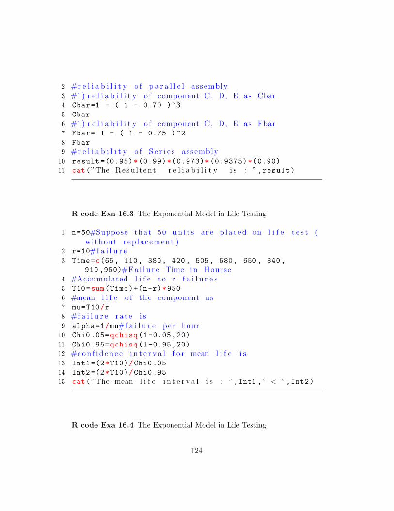
2 #r e l i a b i l i t y o f p a r a l l e l a s sembly3 #1) r e l i a b i l i t y o f component C, D, E as Cbar4 Cbar=1 - ( 1 - 0.70 )^3
5 Cbar
6 #1) r e l i a b i l i t y o f component C, D, E as Fbar7 Fbar= 1 - ( 1 - 0.75 )^2
8 Fbar
9 #r e l i a b i l i t y o f S e r i e s as sembly10 result =(0.95)*(0.99)*(0.973)*(0.9375)*(0.90)
11 cat(”The Re su l t e n t r e l i a b i l i t y i s : ”,result)
R code Exa 16.3 The Exponential Model in Life Testing
1 n=50#Suppose tha t 50 u n i t s a r e p l a c ed on l i f e t e s t (w i thout r ep l a c ement )
2 r=10#f a i l u r e3 Time=c(65, 110, 380, 420, 505, 580, 650, 840,
910 ,950)#Fa i l u r e Time in Hourse4 #Accumulated l i f e to r f a i l u r e s5 T10=sum(Time)+(n-r)*950
6 #mean l i f e o f the component as7 mu=T10/r
8 #f a i l u r e r a t e i s9 alpha=1/mu#f a i l u r e per hour
10 Chi0 .05= qchisq (1 -0.05 ,20)
11 Chi0 .95= qchisq (1 -0.95 ,20)
12 #con f i d e n c e i n t e r v a l f o r mean l i f e i s13 Int1 =(2*T10)/Chi0 .05
14 Int2 =(2*T10)/Chi0 .95
15 cat(”The mean l i f e i n t e r v a l i s : ”,Int1 ,” < ”,Int2)
R code Exa 16.4 The Exponential Model in Life Testing
124
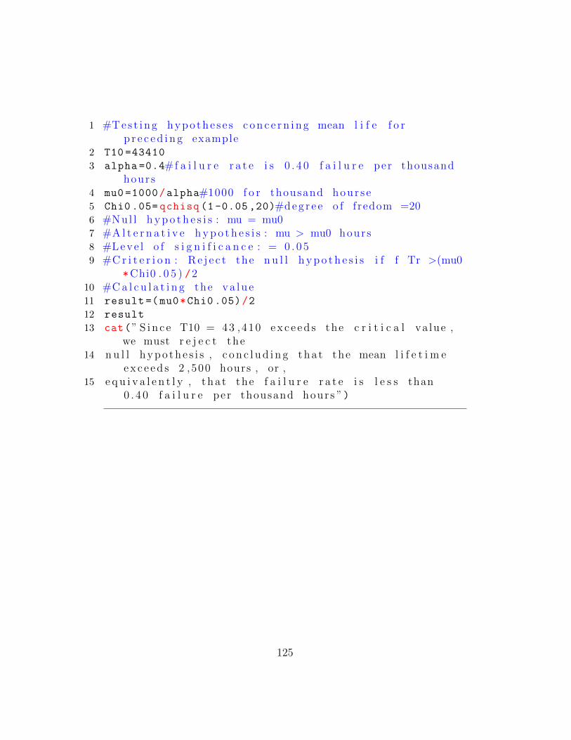
1 #Tes t i ng hypo the s e s c on c e r n i n g mean l i f e f o rp r e c e d i n g example
2 T10 =43410
3 alpha =0.4#f a i l u r e r a t e i s 0 . 4 0 f a i l u r e per thousandhours
4 mu0 =1000/alpha#1000 f o r thousand hour s e5 Chi0 .05= qchisq (1 -0.05 ,20)#deg r e e o f fredom =206 #Nul l h yp o t h e s i s : mu = mu07 #A l t e r n a t i v e h yp o t h e s i s : mu > mu0 hours8 #Leve l o f s i g n i f i c a n c e : = 0 . 0 59 #Cr i t e r i o n : Re j e c t the n u l l h yp o t h e s i s i f f Tr >(mu0
*Chi0 . 0 5 ) /210 #Ca l c u l a t i n g the va lu e11 result =(mu0*Chi0 .05)/2
12 result
13 cat(” S i n c e T10 = 43 ,410 ex c e ed s the c r i t i c a l va lue ,we must r e j e c t the
14 n u l l hypo th e s i s , c on c l ud i n g tha t the mean l i f e t i m eex c e ed s 2 ,500 hours , or ,
15 e q u i v a l e n t l y , tha t the f a i l u r e r a t e i s l e s s than0 . 4 0 f a i l u r e per thousand hours ”)
125