R++, the Next Step

User guide

– Version 1.3 –

~ 2 ~

Contents Quick Start, R++ in a nutshell ................................................................................................................. 4

A typical use case ................................................................................................................................... 5

I. Overview .............................................................................................................................................................. 5

1.1 Installation ................................................................................................................................................. 5

1.2 General concepts ...................................................................................................................................... 5

II Opening your dataset ...................................................................................................................................... 6

2.1 Standard opening .................................................................................................................................... 6

2.2 Copy-Paste data ........................................................................................................................................ 7

III Data management ........................................................................................................................................ 8

3.1 How to deal with outliers ..................................................................................................................... 9

3.2 Correcting categories on type conversion .................................................................................. 10

3.3 Category fusion...................................................................................................................................... 11

3.4 Sorting variables ................................................................................................................................... 11

3.5 Replicating the format of a variable .............................................................................................. 12

3.6 Adding categories ................................................................................................................................. 13

3.7 Discretizing variables ......................................................................................................................... 15

3.8 Filters ........................................................................................................................................................ 15

3.9 The mini report ..................................................................................................................................... 17

3.10 The filmstrip....................................................................................................................................... 17

IV. Data mergers .............................................................................................................................................. 17

4.1 Introduction ............................................................................................................................................ 17

4.2 Merger by column ................................................................................................................................ 18

4.3 Merger by line or individual ............................................................................................................. 21

V Bivariate analysis – Statistical tests ....................................................................................................... 26

5.1 Selecting the reference column ....................................................................................................... 26

5.2 Summary .................................................................................................................................................. 26

5.3 Bivariate graphs .................................................................................................................................... 27

5.4 Statistical tests ....................................................................................................................................... 28

VI. Linear regression, logistic regression and ANOVA ....................................................................... 30

6.1 How to select the variables ............................................................................................................... 31

6.2 Automated selection ............................................................................................................................ 31

6.3 The interactions .................................................................................................................................... 32

6.4 Presentation of the results ................................................................................................................ 33

6.5 Predictions .............................................................................................................................................. 33

6.6 Finalising a model with large databases ..................................................................................... 34

~ 3 ~

6.7 Saving a model ....................................................................................................................................... 34

VII Exporting...................................................................................................................................................... 34

7.1 Editing graphs ........................................................................................................................................ 34

7.2 Legends .................................................................................................................................................... 35

VIII R scripts ........................................................................................................................................................ 36

8.1 Overall presentation ............................................................................................................................ 36

8.2 The script ................................................................................................................................................. 38

8.3 "Code Summary" ................................................................................................................................... 39

~ 4 ~

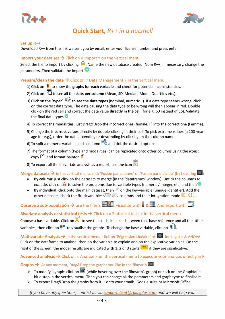
Quick Start, R++ in a nutshell Set up R++ Download R++ from the link we sent you by email, enter your license number and press enter.

Import your data set → Click on « Import » on the vertical menu

Select the file to import by clicking . Name the new database created (Nom R++). If necessary, change the

parameters. Then validate the import .

Prepare/clean the data → Click on « Data Management » in the vertical menu

1) Click on to show the graphs for each variable and check for potential inconsistencies.

2) Click on to see all the stats per column (Mean, SD, Median, Mode, Quartiles etc.).

3) Click on the ‘typer’ to see the data types (nominal, numeric…). If a data type seems wrong, click on the correct data type. The data causing the data type to be wrong will then appear in red. Double click on the red cell and correct the data value directly in the cell (for e.g. 60 instead of 6o). Validate

the final data types .

4) To correct the modalities, just Drag&Drop the incorrect ones (female, F) into the correct one (Femme).

5) Change the incorrect values directly by double-clicking in their cell. To pick extreme values (a 200-year age for e.g.), order the data ascending or descending by clicking on the column name.

6) To split a numeric variable, add a column and tick the desired options.

7) The format of a column (type and modalities) can be replicated onto other columns using the icons:

copy and format-painter .

8) To export all the univariate analysis as a report, use the icon

Merge datasets → in the vertical menu, click ‘Fusion par colonne’ or ‘Fusion par individu’ (by hovering )

• By column: just click on the datasets to merge (in the ‘dataframes’ window). Untick the columns to

exclude, click on to solve the problems due to variable types (numeric / integer, etc) and then

• By individual: click onto the main dataset, then on the key-variable (unique identifier). Add the

other datasets, check the fixed/variables columns and their integration mode …

Observe a sub-population → use the filters , visualise with & . And export with

Bivariate analysis or statistical tests → Click on « Statistical tests » in the vertical menu

Choose a base variable. Click on to see the statistical tests between that base reference and all the other

variables, then click on to visualise the graphs. To change the base variable, click on .

Multivariate Analysis → In the vertical menu, click on ‘Régression Linéaire’ or for Logistic & ANOVA Click on the dataframe to analyse, then on the variable to explain and on the explicative variables. On the

right of the screen, the model results are indicated with 1, 2 or 3 starts if they are significative.

Advanced analysis → Click on « Analyse » on the vertical menu to execute your analysis directly in R

Graphs → At any moment, Drag&Drop the graphs you like in the filmstrip

➢ To modify a graph: click on (while hovering over the filmstrip’s graph) or click on the Graphique blue step in the vertical menu. Then you can change all the parameters and graph type to finalise it.

➢ To export Drag&Drop the graphs from R++ onto your emails, Google suite or Microsoft Office.

If you have any questions, contact us via supportclient@rplusplus.com and we will help you.

~ 5 ~

A typical use case

I. Overview

1.1 Installation ➢ First, click on the link sent to you via email to download R++, then double-click on the

installation icon. ➢ A box is asking if you accept the license. Optionally, you can change the current directory. To

validate, click on Terminer. ➢ Your license code has also been sent to you by email; in case of problem, please contact

supportclient@rplusplus.com. ➢ Once you have entered your license code, R++ is installing, then the software is ready.

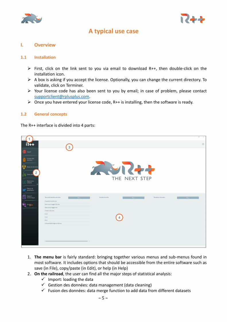
1.2 General concepts The R++ interface is divided into 4 parts:

1. The menu bar is fairly standard: bringing together various menus and sub-menus found in most software. It includes options that should be accessible from the entire software such as save (in File), copy/paste (in Edit), or help (in Help)

2. On the railroad, the user can find all the major steps of statistical analysis: ✓ Import: loading the data ✓ Gestion des données: data management (data cleaning) ✓ Fusion des données: data merge function to add data from different datasets

~ 6 ~

✓ Statistical tests: bivariate analysis ✓ Regressions: linear, logistics and Manova ✓ Export: export and save your results ✓ Script: In addition to the 6 steps, the script allows you to perform more in-depth

analyzes in the R console (machine learning, clustering, etc) 3. The toolbar contains icons specific to each step of the railroad. For example, at the “Import”

step, it is possible to preview the data. At the Data Management step (gestion des données), the types of each column can be displayed.

4. The main view contains, depending on the step, data, codes, scripts, graphs ...

II Opening your dataset

2.1 Standard opening

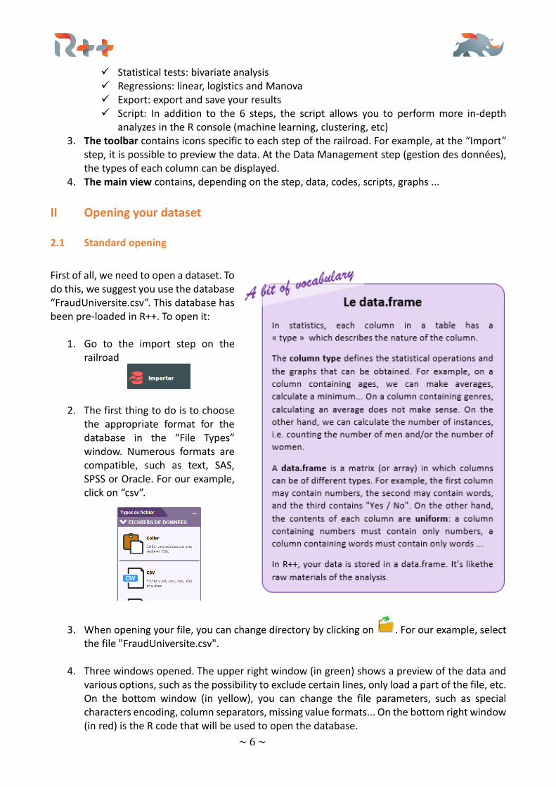
First of all, we need to open a dataset. To do this, we suggest you use the database “FraudUniversite.csv”. This database has been pre-loaded in R++. To open it:

1. Go to the import step on the railroad

2. The first thing to do is to choose the appropriate format for the database in the “File Types” window. Numerous formats are compatible, such as text, SAS, SPSS or Oracle. For our example, click on “csv”.

3. When opening your file, you can change directory by clicking on . For our example, select the file "FraudUniversite.csv".

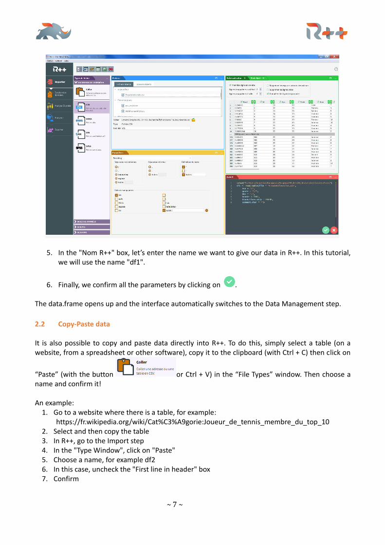
4. Three windows opened. The upper right window (in green) shows a preview of the data and

various options, such as the possibility to exclude certain lines, only load a part of the file, etc. On the bottom window (in yellow), you can change the file parameters, such as special characters encoding, column separators, missing value formats... On the bottom right window (in red) is the R code that will be used to open the database.

~ 7 ~

5. In the "Nom R++" box, let’s enter the name we want to give our data in R++. In this tutorial, we will use the name "df1".

6. Finally, we confirm all the parameters by clicking on . The data.frame opens up and the interface automatically switches to the Data Management step.

2.2 Copy-Paste data It is also possible to copy and paste data directly into R++. To do this, simply select a table (on a website, from a spreadsheet or other software), copy it to the clipboard (with Ctrl + C) then click on

“Paste” (with the button or Ctrl + V) in the “File Types” window. Then choose a name and confirm it! An example:

1. Go to a website where there is a table, for example: https://fr.wikipedia.org/wiki/Cat%C3%A9gorie:Joueur_de_tennis_membre_du_top_10

2. Select and then copy the table 3. In R++, go to the Import step 4. In the "Type Window", click on "Paste" 5. Choose a name, for example df2 6. In this case, uncheck the "First line in header" box 7. Confirm

~ 8 ~

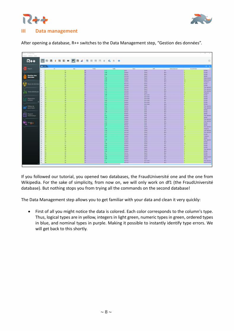
III Data management After opening a database, R++ switches to the Data Management step, “Gestion des données”.

If you followed our tutorial, you opened two databases, the FraudUniversité one and the one from Wikipedia. For the sake of simplicity, from now on, we will only work on df1 (the FraudUniversité database). But nothing stops you from trying all the commands on the second database! The Data Management step allows you to get familiar with your data and clean it very quickly:

• First of all you might notice the data is colored. Each color corresponds to the column's type. Thus, logical types are in yellow, integers in light green, numeric types in green, ordered types in blue, and nominal types in purple. Making it possible to instantly identify type errors. We will get back to this shortly.

~ 9 ~

• The summary button shows the average, the standard deviation, and the quartiles of integer and numeric variables, as well as the count of logical, ordered and nominal variables.

Note, if you want to export the results of the Summaries to another software,

simply copy-paste: click on (this copies the summary), open Excel or another software then paste it (Ctrl+V). Two remarks: — The counts of the nominal variables

are given in descending order: the category with the largest number first.

— If there are many different modalities, only the first 200 are given

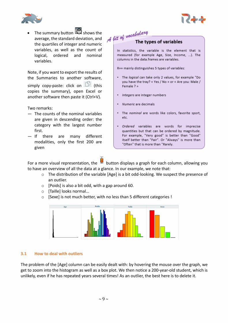
For a more visual representation, the button displays a graph for each column, allowing you to have an overview of all the data at a glance. In our example, we note that:

o The distribution of the variable [Age] is a bit odd-looking. We suspect the presence of an outlier.

o [Poids] is also a bit odd, with a gap around 60. o [Taille] looks normal… o [Sexe] is not much better, with no less than 5 different categories !

3.1 How to deal with outliers

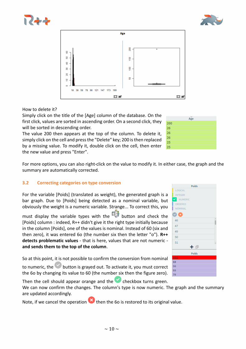
The problem of the [Age] column can be easily dealt with: by hovering the mouse over the graph, we get to zoom into the histogram as well as a box plot. We then notice a 200-year-old student, which is unlikely, even if he has repeated years several times! As an outlier, the best here is to delete it.

~ 10 ~

How to delete it? Simply click on the title of the [Age] column of the database. On the first click, values are sorted in ascending order. On a second click, they will be sorted in descending order. The value 200 then appears at the top of the column. To delete it, simply click on the cell and press the "Delete" key; 200 is then replaced by a missing value. To modify it, double click on the cell, then enter the new value and press "Enter". For more options, you can also right-click on the value to modify it. In either case, the graph and the summary are automatically corrected.

3.2 Correcting categories on type conversion

For the variable [Poids] (translated as weight), the generated graph is a bar graph. Due to [Poids] being detected as a nominal variable, but obviously the weight is a numeric variable. Strange... To correct this, you

must display the variable types with the button and check the [Poids] column : indeed, R++ didn't give it the right type initially because in the column [Poids], one of the values is nominal. Instead of 60 (six and then zero), it was entered 6o (the number six then the letter "o"). R++ detects problematic values - that is here, values that are not numeric - and sends them to the top of the column.

So at this point, it is not possible to confirm the conversion from nominal

to numeric, the button is grayed out. To activate it, you must correct the 6o by changing its value to 60 (the number six then the figure zero).

Then the cell should appear orange and the checkbox turns green. We can now confirm the changes. The column's type is now numeric. The graph and the summary are updated accordingly.

Note, if we cancel the operation then the 6o is restored to its original value.

~ 11 ~

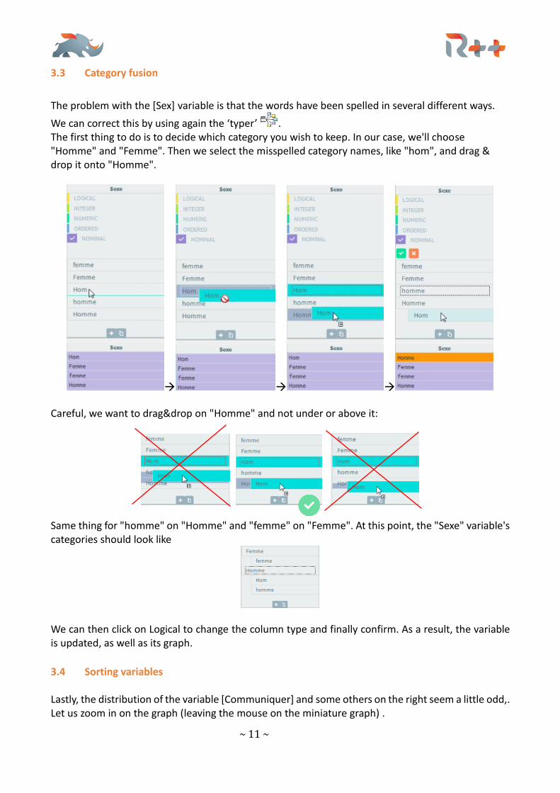
3.3 Category fusion

The problem with the [Sex] variable is that the words have been spelled in several different ways.

We can correct this by using again the ‘typer’ . The first thing to do is to decide which category you wish to keep. In our case, we'll choose "Homme" and "Femme". Then we select the misspelled category names, like "hom", and drag & drop it onto "Homme".

→ → →

Careful, we want to drag&drop on "Homme" and not under or above it:

Same thing for "homme" on "Homme" and "femme" on "Femme". At this point, the "Sexe" variable's categories should look like

We can then click on Logical to change the column type and finally confirm. As a result, the variable is updated, as well as its graph.

3.4 Sorting variables Lastly, the distribution of the variable [Communiquer] and some others on the right seem a little odd,. Let us zoom in on the graph (leaving the mouse on the miniature graph) .

~ 12 ~

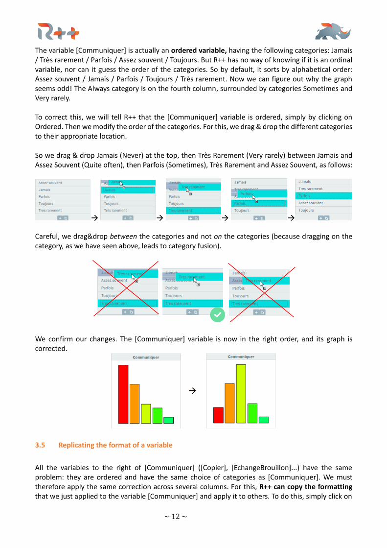
The variable [Communiquer] is actually an ordered variable, having the following categories: Jamais / Très rarement / Parfois / Assez souvent / Toujours. But R++ has no way of knowing if it is an ordinal variable, nor can it guess the order of the categories. So by default, it sorts by alphabetical order: Assez souvent / Jamais / Parfois / Toujours / Très rarement. Now we can figure out why the graph seems odd! The Always category is on the fourth column, surrounded by categories Sometimes and Very rarely. To correct this, we will tell R++ that the [Communiquer] variable is ordered, simply by clicking on Ordered. Then we modify the order of the categories. For this, we drag & drop the different categories to their appropriate location. So we drag & drop Jamais (Never) at the top, then Très Rarement (Very rarely) between Jamais and Assez Souvent (Quite often), then Parfois (Sometimes), Très Rarement and Assez Souvent, as follows:

→ → → →

Careful, we drag&drop between the categories and not on the categories (because dragging on the category, as we have seen above, leads to category fusion).

We confirm our changes. The [Communiquer] variable is now in the right order, and its graph is corrected.

3.5 Replicating the format of a variable

All the variables to the right of [Communiquer] ([Copier], [EchangeBrouillon]...) have the same problem: they are ordered and have the same choice of categories as [Communiquer]. We must therefore apply the same correction across several columns. For this, R++ can copy the formatting that we just applied to the variable [Communiquer] and apply it to others. To do this, simply click on

~ 13 ~

the "copy format" button . This turns all the "copy format" buttons of the other columns into

"paste format" . Then click on "paste format" in the column [EchangeBrouillon]. The variable orders itself properly and the categories are corrected. The same can be done for [Copier],

[Antiseche], and all other columns. When we have just done a "paste format" on a column, the

button changes to finish copy-and-paste formats" . When we want to stop pasting formats, we

can simply click on any .

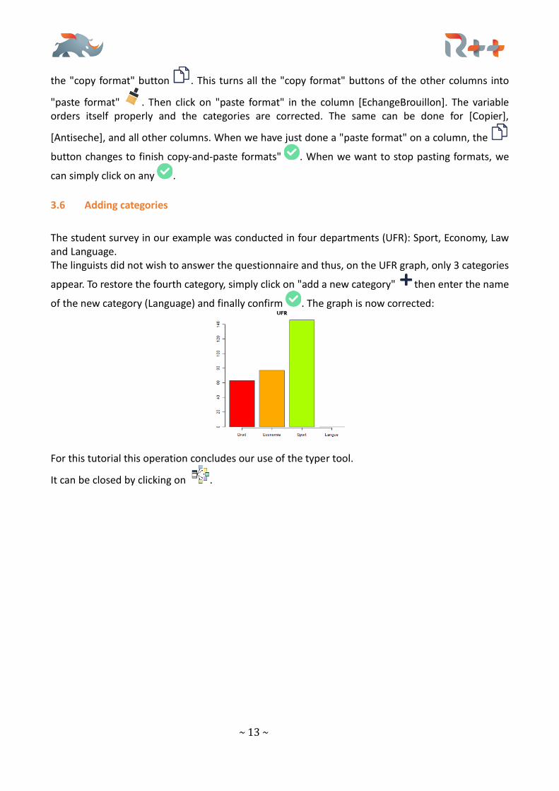
3.6 Adding categories

The student survey in our example was conducted in four departments (UFR): Sport, Economy, Law and Language. The linguists did not wish to answer the questionnaire and thus, on the UFR graph, only 3 categories

appear. To restore the fourth category, simply click on "add a new category" then enter the name

of the new category (Language) and finally confirm . The graph is now corrected:

For this tutorial this operation concludes our use of the typer tool.

It can be closed by clicking on .

~ 14 ~

~ 15 ~

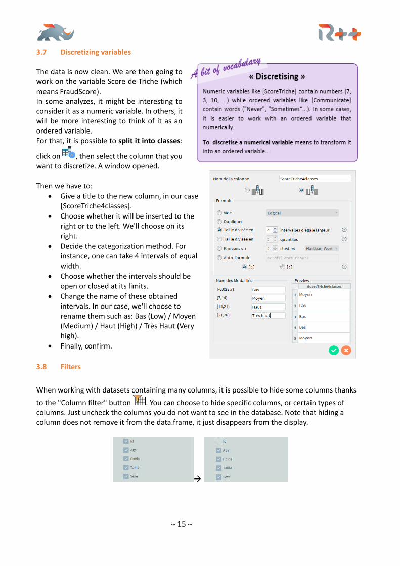
3.7 Discretizing variables The data is now clean. We are then going to work on the variable Score de Triche (which means FraudScore). In some analyzes, it might be interesting to consider it as a numeric variable. In others, it will be more interesting to think of it as an ordered variable. For that, it is possible to split it into classes:

click on , then select the column that you want to discretize. A window opened. Then we have to:

• Give a title to the new column, in our case [ScoreTriche4classes].

• Choose whether it will be inserted to the right or to the left. We'll choose on its right.

• Decide the categorization method. For instance, one can take 4 intervals of equal width.

• Choose whether the intervals should be open or closed at its limits.

• Change the name of these obtained intervals. In our case, we'll choose to rename them such as: Bas (Low) / Moyen (Medium) / Haut (High) / Très Haut (Very high).

• Finally, confirm.

3.8 Filters

When working with datasets containing many columns, it is possible to hide some columns thanks

to the "Column filter" button . You can choose to hide specific columns, or certain types of columns. Just uncheck the columns you do not want to see in the database. Note that hiding a column does not remove it from the data.frame, it just disappears from the display.

→

~ 16 ~

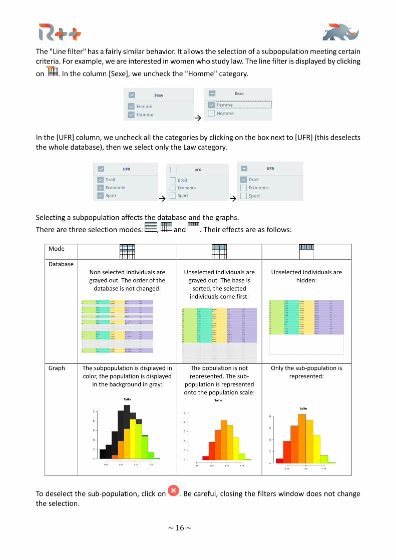
The "Line filter" has a fairly similar behavior. It allows the selection of a subpopulation meeting certain criteria. For example, we are interested in women who study law. The line filter is displayed by clicking

on . In the column [Sexe], we uncheck the "Homme" category.

→ In the [UFR] column, we uncheck all the categories by clicking on the box next to [UFR] (this deselects the whole database), then we select only the Law category.

→ →

Selecting a subpopulation affects the database and the graphs.

There are three selection modes: , and . Their effects are as follows:

Mode

Database

Non selected individuals are grayed out. The order of the

database is not changed:

Unselected individuals are

grayed out. The base is sorted, the selected

individuals come first:

Unselected individuals are

hidden:

Graph The subpopulation is displayed in color, the population is displayed

in the background in gray:

The population is not represented. The sub-

population is represented onto the population scale:

Only the sub-population is represented:

To deselect the sub-population, click on . Be careful, closing the filters window does not change the selection.

~ 17 ~

3.9 The mini report

R++ allows you to automatically create a "mini report" on the univariate analysis. You will thus be able to have all the summaries of each variable as well as their graphic representation in a single document.

• Click on . A window opens with all the report parameters: • Choose the name and the format (html, word or pdf) of the report. • The data to be exported allows you to choose the elements that should appear in the

report. You can then decide which variables should be selected. For example, "Columns displayed" will export all columns except those that have been deselected via the column filter.

• When you validate, a report containing the requested information is created.

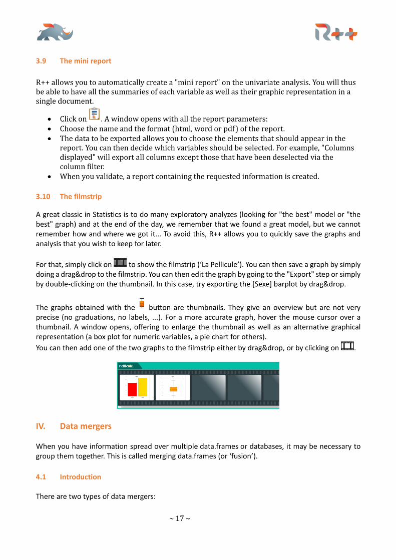
3.10 The filmstrip

A great classic in Statistics is to do many exploratory analyzes (looking for "the best" model or "the best" graph) and at the end of the day, we remember that we found a great model, but we cannot remember how and where we got it... To avoid this, R++ allows you to quickly save the graphs and analysis that you wish to keep for later.

For that, simply click on to show the filmstrip (‘La Pellicule’). You can then save a graph by simply doing a drag&drop to the filmstrip. You can then edit the graph by going to the "Export" step or simply by double-clicking on the thumbnail. In this case, try exporting the [Sexe] barplot by drag&drop.

The graphs obtained with the button are thumbnails. They give an overview but are not very precise (no graduations, no labels, ...). For a more accurate graph, hover the mouse cursor over a thumbnail. A window opens, offering to enlarge the thumbnail as well as an alternative graphical representation (a box plot for numeric variables, a pie chart for others).

You can then add one of the two graphs to the filmstrip either by drag&drop, or by clicking on .

IV. Data mergers When you have information spread over multiple data.frames or databases, it may be necessary to group them together. This is called merging data.frames (or ‘fusion’).

4.1 Introduction There are two types of data mergers:

~ 18 ~

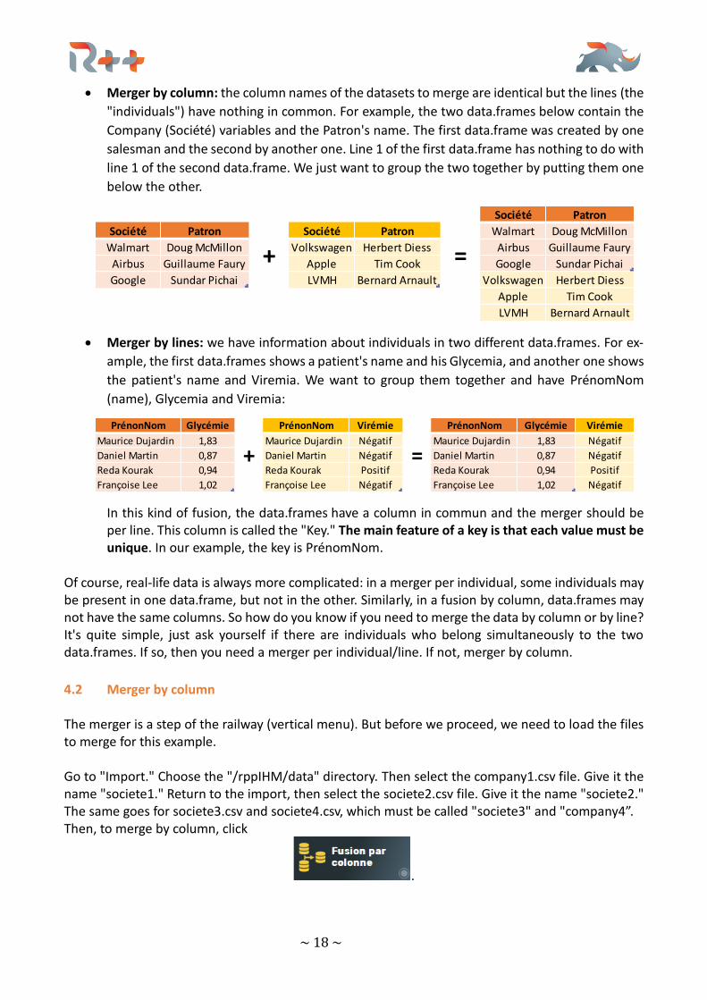
• Merger by column: the column names of the datasets to merge are identical but the lines (the

"individuals") have nothing in common. For example, the two data.frames below contain the

Company (Société) variables and the Patron's name. The first data.frame was created by one

salesman and the second by another one. Line 1 of the first data.frame has nothing to do with

line 1 of the second data.frame. We just want to group the two together by putting them one

below the other.

• Merger by lines: we have information about individuals in two different data.frames. For ex-

ample, the first data.frames shows a patient's name and his Glycemia, and another one shows

the patient's name and Viremia. We want to group them together and have PrénomNom

(name), Glycemia and Viremia:

In this kind of fusion, the data.frames have a column in commun and the merger should be per line. This column is called the "Key." The main feature of a key is that each value must be unique. In our example, the key is PrénomNom.

Of course, real-life data is always more complicated: in a merger per individual, some individuals may be present in one data.frame, but not in the other. Similarly, in a fusion by column, data.frames may not have the same columns. So how do you know if you need to merge the data by column or by line? It's quite simple, just ask yourself if there are individuals who belong simultaneously to the two data.frames. If so, then you need a merger per individual/line. If not, merger by column.

4.2 Merger by column The merger is a step of the railway (vertical menu). But before we proceed, we need to load the files to merge for this example. Go to "Import." Choose the "/rppIHM/data" directory. Then select the company1.csv file. Give it the name "societe1." Return to the import, then select the societe2.csv file. Give it the name "societe2." The same goes for societe3.csv and societe4.csv, which must be called "societe3" and "company4”. Then, to merge by column, click

.

Société Patron

Société Patron Société Patron Walmart Doug McMillon

Walmart Doug McMillon Volkswagen Herbert Diess Airbus Guillaume Faury

Airbus Guillaume Faury Apple Tim Cook Google Sundar Pichai

Google Sundar Pichai LVMH Bernard Arnault Volkswagen Herbert Diess

Apple Tim Cook

LVMH Bernard Arnault

+ =

PrénonNom Glycémie PrénonNom Virémie PrénonNom Glycémie Virémie

Maurice Dujardin 1,83 Maurice Dujardin Négatif Maurice Dujardin 1,83 Négatif

Daniel Martin 0,87 Daniel Martin Négatif Daniel Martin 0,87 Négatif

Reda Kourak 0,94 Reda Kourak Positif Reda Kourak 0,94 Positif

Françoise Lee 1,02 Françoise Lee Négatif Françoise Lee 1,02 Négatif

+ =

~ 19 ~

4.2.1 Selecting the datasets The list of data.frames in memory is displayed on the left, in the purple window. If you have followed this tutorial, there are 6 data.frames: dn1, dn2, societe1, societe2, societe3 and societe4. On the right, the blue window allows you to get a glimpse of the merged data.frame. To merge two data.frames per column, choose your data.frames by clicking on their names in the purple window. In this case, choose societe1. The data.frame appears on the right side, in the blue window. Then select societe2. It comes by itself in the blue window under the first data.frame.

In a column fusion, each line comes from a single data.frame. It keeps track of the provenance of each line by automatically adding a "SourceFusion" column. This column contains the name of the data.frame from which the line originates. If you don't want this column to be present in the merged data.frame, you can simply uncheck it by clicking on the column head. It also uses a color system to indicate where each value comes from. In the data.frame (violet) window, selected data.frames are coloured. The first base is orange, the next ones are yellow. In the preview window, data from a particular data.frame is also colored, according to the same color code. In our case, the data from societe1 are orange, the societe2 data are in yellow.

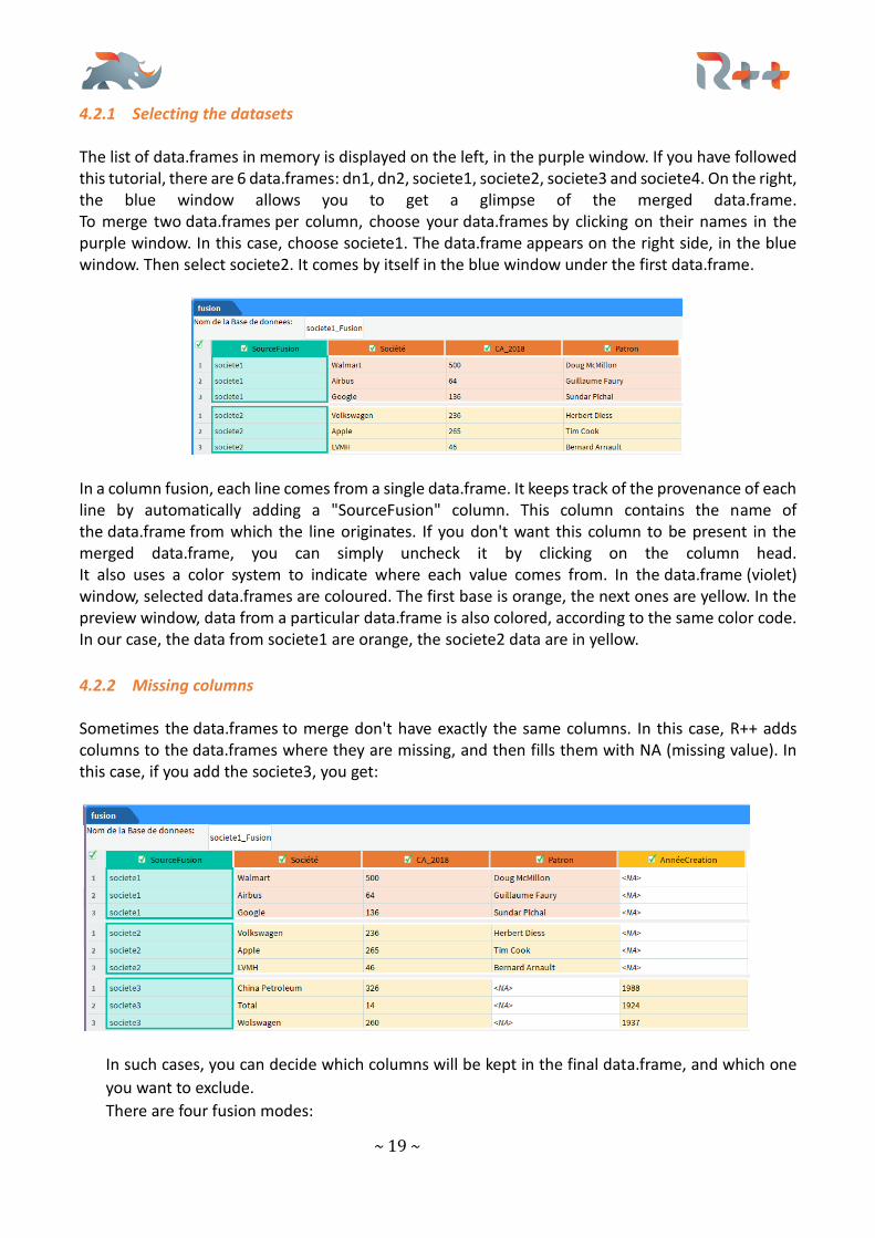
4.2.2 Missing columns Sometimes the data.frames to merge don't have exactly the same columns. In this case, R++ adds columns to the data.frames where they are missing, and then fills them with NA (missing value). In this case, if you add the societe3, you get:

In such cases, you can decide which columns will be kept in the final data.frame, and which one

you want to exclude.

There are four fusion modes:

~ 20 ~

• to select all the columns of all data.frames. On the example above: SourceFusion, So-

ciété, CA_2018, Patron et AnnéeCréation

• to select the columns of the first data.frame. On the example : SourceFusion, Société,

CA_2018 et Patron

• to select all the columns of data.frames two, three and following, but does not add the

ones that are specific to the first.

• to select only columns that are common to all data.frames. On the example: Source-

Fusion, Société et CA_2018

When you select one or the other mode (listed above), you hide the columns that are not affected by

the fusion mode. It is then possible to individually refine and delete certain columns by clicking on the head of the column. In this case, the column is simply grayed out. It is possible to exclude or re-

include all columns by clicking on , at the top left of the merged data.frame.

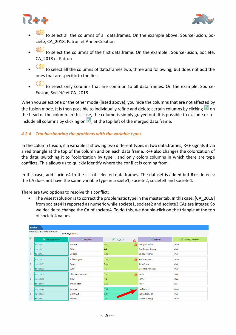
4.2.4 Troubleshooting the problems with the variable types In the column fusion, if a variable is showing two different types in two data.frames, R++ signals it via a red triangle at the top of the column and on each data.frame. R++ also changes the colorization of the data: switching it to "colorization by type", and only colors columns in which there are type conflicts. This allows us to quickly identify where the conflict is coming from. In this case, add societe4 to the list of selected data.frames. The dataset is added but R++ detects: the CA does not have the same variable type in societe1, societe2, societe3 and societe4. There are two options to resolve this conflict:

• The wisest solution is to correct the problematic type in the master tab. In this case, [CA_2018] from societe4 is reported as numeric while societe1, societe2 and societe3 CAs are integer. So we decide to change the CA of societe4. To do this, we double-click on the triangle at the top of societe4 values.

~ 21 ~

• The Data Management tab is now opened. The dataset societe4 comes to the front and the

‘typeur’ opens. Now you can select ‘integer’. The value 30.1 for microsoft’s CA goes up to the

top of the column. Change it to 30, then validate. You can then return to the ‘fusion’ tab. The

warning on the [CA_2018] column is gone.

• You can also decide to ignore the warning. When you validate the merger, the type of column will be automatically determined by R++ according to the "most frequent type" principle:

o If the conflict is between integer and numeric, the type will be numeric

o In all other cases, the type will be nominal.

4.2.5 Finalisation By default, the merged base gets the name of the first selected base to which it adds "_Fusion." So in this case, you get [societe1_Fusion]; you can change it to [SocietesToutes]. When all the dataframes have been selected and conflicts are resolved, you can validate by clicking

. The interface switches to the next step, which is data management, in the ‘Gestion des Données’ tab.

4.3 Merger by line or individual

4.3.1 Variables of different natures In a merger per individual, the variables can be of different natures:

• The "key" is a variable that contains a unique identifier. It can be a name, a number, a code... This identifier will define the lines that need to be merged between them. A Maurice Dujardin line from the first dataset will be merged with the Maurice Dujardin line from the second base. For this, a key variable must have two properties:

o Unique values: all values of the key variable of a data.frame must be different from each other. In other words, a given data.frame can only contain one Maurice Dujardin.

o Common existence: in the context of a merger by individual, the key must therefore exist in all data.frames that will be merged. In other words, if the key is the [PrenomNom] variable, only data.frame with a [NomPrenom] variable can be added.

• "Fixed" variables are variables that, for a given individual, do not change value. For example, the eye color does not change from one day to another. For a given individual, [CouleurDesYeux] is therefore a fixed variable.

• On the other hand, if the variable values can change from one dataframe to another, we know it is a "variable" variable. In the merged database, variable variables must be present as many times as the number of dataframes.

As an example… Maurice Dujardin does several analyzes at the hospital. In the morning, a virologist asks him his name, his size and notes in the third column his level of viremia. In the afternoon, an endocrinologist asks

~ 22 ~

him his name, his height and notes his blood sugar level in the third column. The variable ‘taille de Maurice’ is present in both databases. But in the fusion base, it should only be present in a single copy because it is unlikely that Maurice's height (taille) will change between morning and afternoon! It is a fixed variable. After this first day, which took place in January, Maurice measures his blood sugar level in February and in March. We want to merge January, February and March, because we are interested in the variation of the blood sugar variable over time. In the merged database, we want the blood sugar level written in three columns (Jan, Feb, Mar). The blood sugar variable is a variable variable. Note: the fixed or variable nature of a variable depends on the context. For example, height in adults is fixed while it is variable in children; the weight is variable unless it has been measured twice on the same day; sex is fixed except in a survey of “unconventional” sexualities which would include transsexuals; And so on.

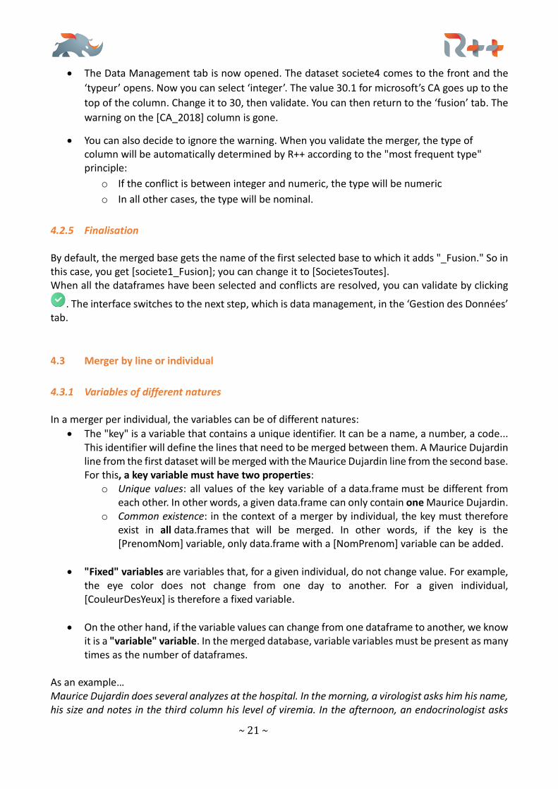
4.3.2 How to select the main dataframe and the key Go back to the Import tab and open the files patient_january1, patient_january2, patient_february and patient_mars. Call them January1, January2, February and March. Next, you need to open the ‘Fusion par individu’ window. By default, the merge by column is showing (‘Fusion par colonne’). To open the merger by individual (‘Fusion par individu’), click on the small circle and click on ‘Fusion par individu’.

→ → → Making this choice changes the railroad: the Railroad Fusion step is now an individual merge. Next, can you see the databases on the left? Click on the january1 database. It opens on the right.

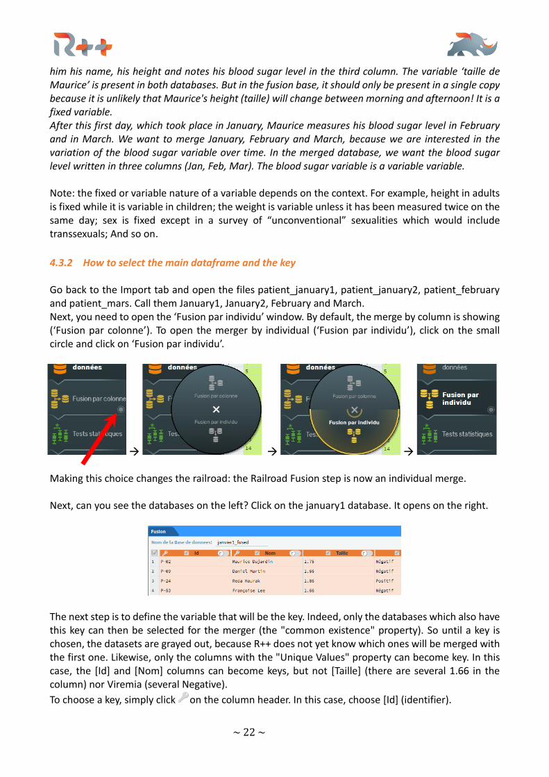
The next step is to define the variable that will be the key. Indeed, only the databases which also have this key can then be selected for the merger (the "common existence" property). So until a key is chosen, the datasets are grayed out, because R++ does not yet know which ones will be merged with the first one. Likewise, only the columns with the "Unique Values" property can become key. In this case, the [Id] and [Nom] columns can become keys, but not [Taille] (there are several 1.66 in the column) nor Viremia (several Negative).

To choose a key, simply click on the column header. In this case, choose [Id] (identifier).

~ 23 ~

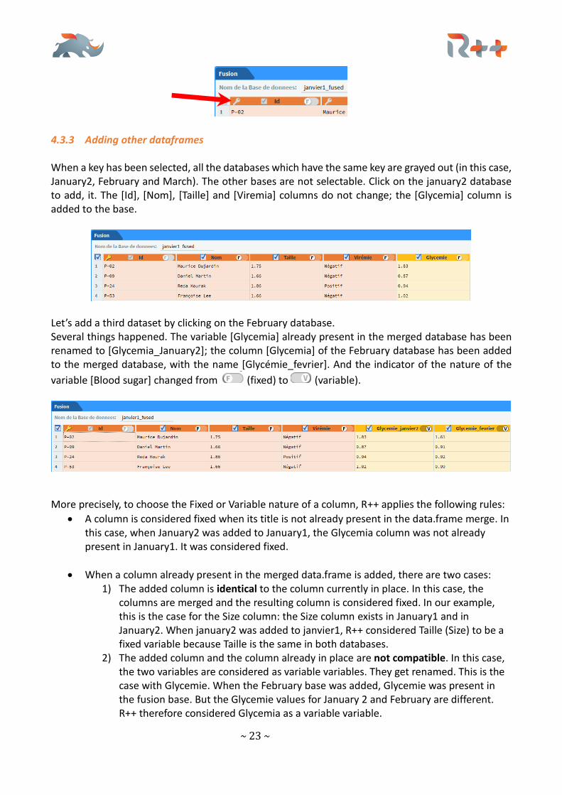
4.3.3 Adding other dataframes When a key has been selected, all the databases which have the same key are grayed out (in this case, January2, February and March). The other bases are not selectable. Click on the january2 database to add, it. The [Id], [Nom], [Taille] and [Viremia] columns do not change; the [Glycemia] column is added to the base.

Let’s add a third dataset by clicking on the February database. Several things happened. The variable [Glycemia] already present in the merged database has been renamed to [Glycemia_January2]; the column [Glycemia] of the February database has been added to the merged database, with the name [Glycémie_fevrier]. And the indicator of the nature of the

variable [Blood sugar] changed from (fixed) to (variable).

More precisely, to choose the Fixed or Variable nature of a column, R++ applies the following rules:

• A column is considered fixed when its title is not already present in the data.frame merge. In this case, when January2 was added to January1, the Glycemia column was not already present in January1. It was considered fixed.

• When a column already present in the merged data.frame is added, there are two cases: 1) The added column is identical to the column currently in place. In this case, the

columns are merged and the resulting column is considered fixed. In our example, this is the case for the Size column: the Size column exists in January1 and in January2. When january2 was added to janvier1, R++ considered Taille (Size) to be a fixed variable because Taille is the same in both databases.

2) The added column and the column already in place are not compatible. In this case, the two variables are considered as variable variables. They get renamed. This is the case with Glycemie. When the February base was added, Glycemie was present in the fusion base. But the Glycemie values for January 2 and February are different. R++ therefore considered Glycemia as a variable variable.

~ 24 ~

Some additional remarks:

• At any time, you can decide to modify the R++ defaults by clicking on or . If you do so, your choices will take priority over R++'s automatic choices. In this case, the icons will

change to or , with a small human silhouette indicating that it is your choice.

• The nature of a variable is common to all variables with the same name: it is not possible for Name to be fixed for January1 and January2, variable for February and March. Also, when a variable is defined as a variable, the symbol is common to all the variables concerned.

• There are two ways of ordering variable variables: either they are re-grouped by variable (below left), or by data.frames (below, right). Switching from one mode to another is done by clicking on the or buttons.

4.3.4 Managing conflicts It can happen that the information found in different data.frames about the same fixed variable is contradictory. Usually, this is a simple entry error. When this happens, the first step is to tell R++ that the variable is fixed. R++ then does several things:

• It transforms the variable into a fixed variable

• It signals that there is a conflict by coloring the problem box or boxes in red and adding a tri-angle in the column header.

• In the absence of additional information, R++ considers that the first database is more relia-ble than the second one, itself more reliable than the third one, and so on.

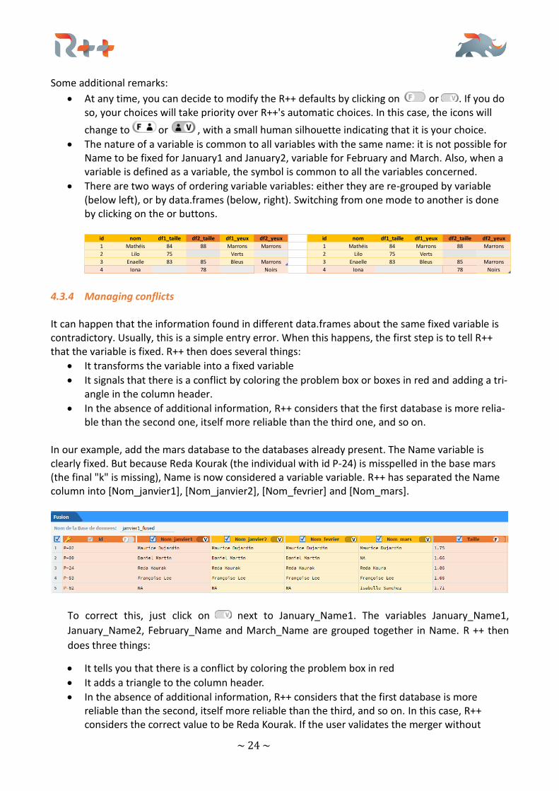
In our example, add the mars database to the databases already present. The Name variable is clearly fixed. But because Reda Kourak (the individual with id P-24) is misspelled in the base mars (the final "k" is missing), Name is now considered a variable variable. R++ has separated the Name column into [Nom_janvier1], [Nom_janvier2], [Nom_fevrier] and [Nom_mars].

To correct this, just click on next to January_Name1. The variables January_Name1,

January_Name2, February_Name and March_Name are grouped together in Name. R ++ then

does three things:

• It tells you that there is a conflict by coloring the problem box in red

• It adds a triangle to the column header.

• In the absence of additional information, R++ considers that the first database is more reliable than the second, itself more reliable than the third, and so on. In this case, R++ considers the correct value to be Reda Kourak. If the user validates the merger without

id nom df1_taille df2_taille df1_yeux df2_yeux id nom df1_taille df1_yeux df2_taille df2_yeux

1 Mathéis 84 88 Marrons Marrons 1 Mathéis 84 Marrons 88 Marrons

2 Lilo 75 Verts 2 Lilo 75 Verts

3 Enaelle 83 85 Bleus Marrons 3 Enaelle 83 Bleus 85 Marrons

4 Iona 78 Noirs 4 Iona 78 Noirs

~ 25 ~

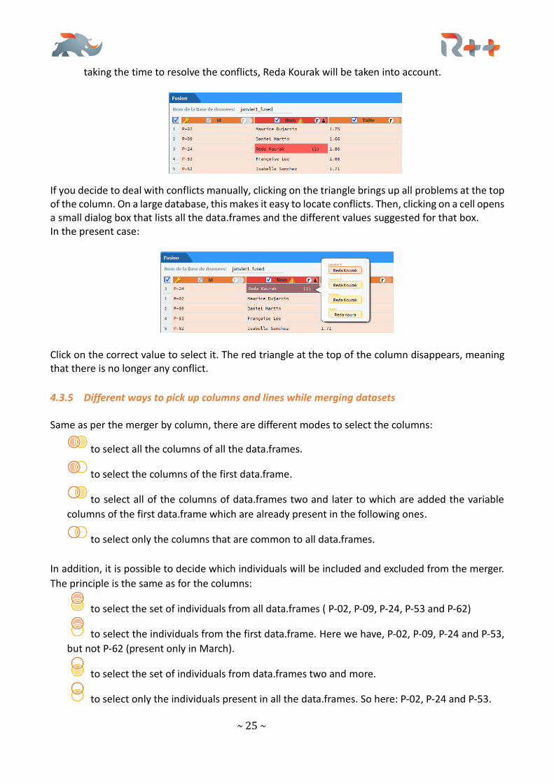
taking the time to resolve the conflicts, Reda Kourak will be taken into account.

If you decide to deal with conflicts manually, clicking on the triangle brings up all problems at the top of the column. On a large database, this makes it easy to locate conflicts. Then, clicking on a cell opens a small dialog box that lists all the data.frames and the different values suggested for that box. In the present case:

Click on the correct value to select it. The red triangle at the top of the column disappears, meaning that there is no longer any conflict.

4.3.5 Different ways to pick up columns and lines while merging datasets Same as per the merger by column, there are different modes to select the columns:

to select all the columns of all the data.frames.

to select the columns of the first data.frame.

to select all of the columns of data.frames two and later to which are added the variable

columns of the first data.frame which are already present in the following ones.

to select only the columns that are common to all data.frames.

In addition, it is possible to decide which individuals will be included and excluded from the merger.

The principle is the same as for the columns:

to select the set of individuals from all data.frames ( P-02, P-09, P-24, P-53 and P-62)

to select the individuals from the first data.frame. Here we have, P-02, P-09, P-24 and P-53,

but not P-62 (present only in March).

to select the set of individuals from data.frames two and more.

to select only the individuals present in all the data.frames. So here: P-02, P-24 and P-53.

~ 26 ~

V Bivariate analysis – Statistical tests The data is ready, cleaned and we're getting to know it a bit better. It is time to move to bivariate analysis. To do this, simply click on the third step on the railroad.

5.1 Selecting the reference column

The first thing to do in bivariate analysis is to choose a reference column to compare with. To do this, simply click on the title of a column. The column then moves from the database to the left side of the view. In our case, we'll choose the reference column [ScoreTriche].

If we then want to change the reference column to another, we’ll just click on the button: the current reference variable returns to the database and we can choose another one by simply clicking on another column title.

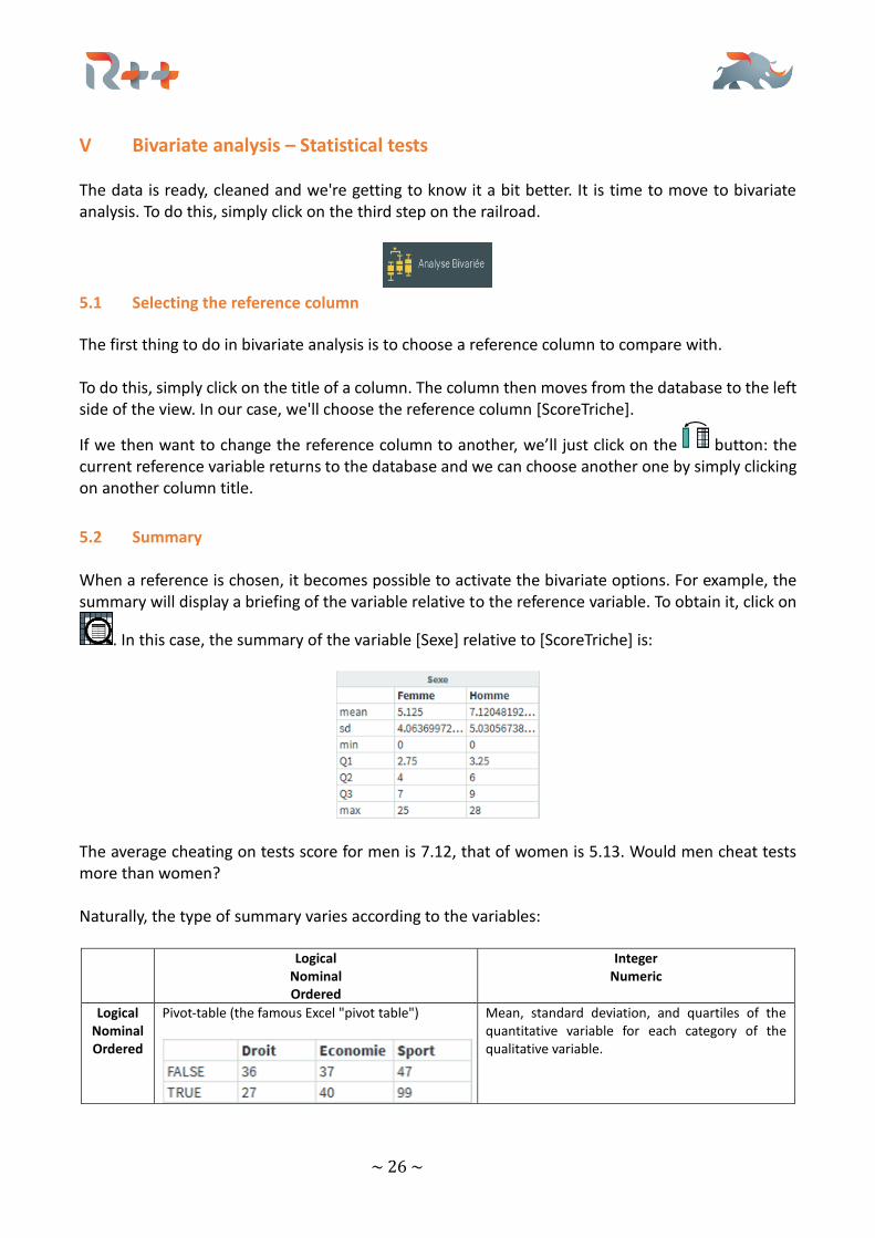
5.2 Summary When a reference is chosen, it becomes possible to activate the bivariate options. For example, the summary will display a briefing of the variable relative to the reference variable. To obtain it, click on

. In this case, the summary of the variable [Sexe] relative to [ScoreTriche] is:

The average cheating on tests score for men is 7.12, that of women is 5.13. Would men cheat tests more than women? Naturally, the type of summary varies according to the variables:

Logical Nominal Ordered

Integer Numeric

Logical Nominal Ordered

Pivot-table (the famous Excel "pivot table")

Mean, standard deviation, and quartiles of the quantitative variable for each category of the qualitative variable.

~ 27 ~

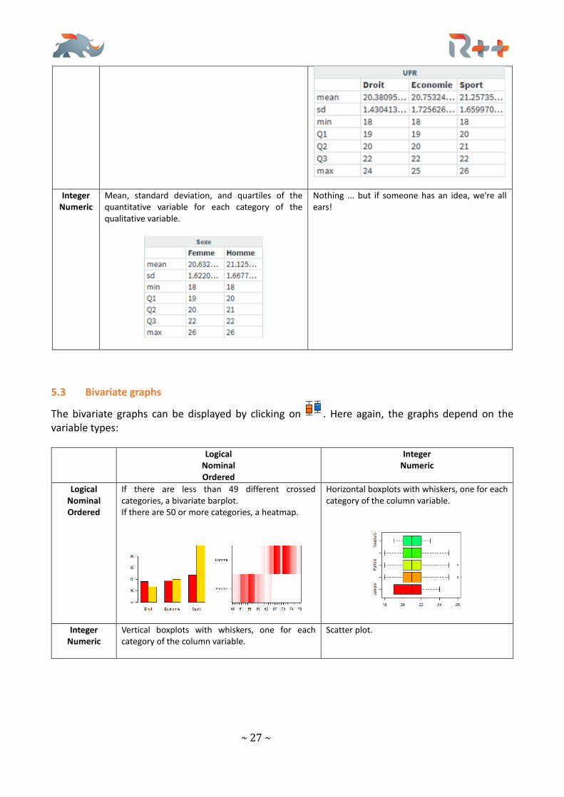
Integer Numeric

Mean, standard deviation, and quartiles of the quantitative variable for each category of the qualitative variable.

Nothing ... but if someone has an idea, we're all ears!

5.3 Bivariate graphs

The bivariate graphs can be displayed by clicking on . Here again, the graphs depend on the variable types:

Logical Nominal Ordered

Integer Numeric

Logical Nominal Ordered

If there are less than 49 different crossed categories, a bivariate barplot. If there are 50 or more categories, a heatmap.

Horizontal boxplots with whiskers, one for each category of the column variable.

Integer Numeric

Vertical boxplots with whiskers, one for each category of the column variable.

Scatter plot.

~ 28 ~

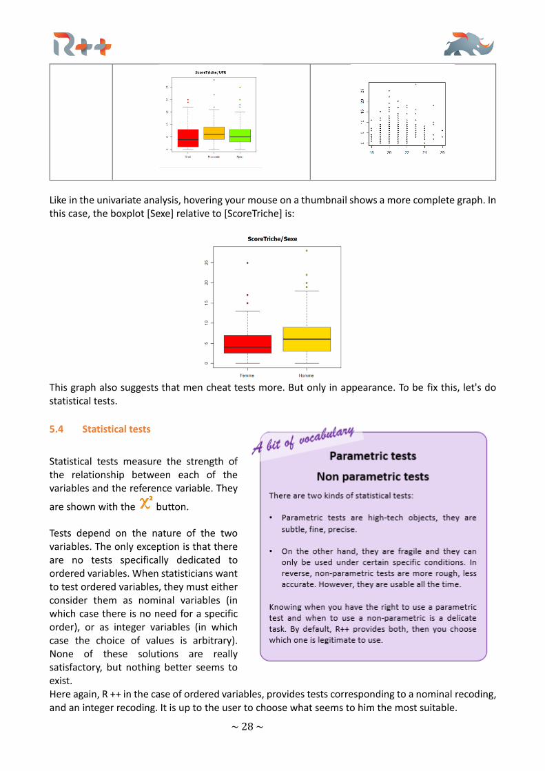
Like in the univariate analysis, hovering your mouse on a thumbnail shows a more complete graph. In this case, the boxplot [Sexe] relative to [ScoreTriche] is:

This graph also suggests that men cheat tests more. But only in appearance. To be fix this, let's do statistical tests.

5.4 Statistical tests

Statistical tests measure the strength of the relationship between each of the variables and the reference variable. They

are shown with the button. Tests depend on the nature of the two variables. The only exception is that there are no tests specifically dedicated to ordered variables. When statisticians want to test ordered variables, they must either consider them as nominal variables (in which case there is no need for a specific order), or as integer variables (in which case the choice of values is arbitrary). None of these solutions are really satisfactory, but nothing better seems to exist. Here again, R ++ in the case of ordered variables, provides tests corresponding to a nominal recoding, and an integer recoding. It is up to the user to choose what seems to him the most suitable.

~ 29 ~

In the end, the list of possible tests is as follows: Logical

Nominal or Ordered to 2 classes

Integer Numeric

Ordered to 3 classes or more

Nominal to 3 classes or more

Logical Nominal or Ordered

to 2 classes

Khi² Fisher's exact test

Integer Numeric

Student's T test Wilcoxon rank test

Spearman's R test Pearson's R test

Ordered to 3 classes or more

Khi² Fisher's exact test Wilcoxon rank test

ANOVA Kruskal Wallis Pearson's R test

Khi² Fisher's exact test Kruskal Wallis Pearson's R test

Nominal to 3 classes or more

Khi² Fisher's exact test

ANOVA Kruskal Wallis

Khi² Fisher's exact test Kruskal Wallis

Khi² Fisher's exact test

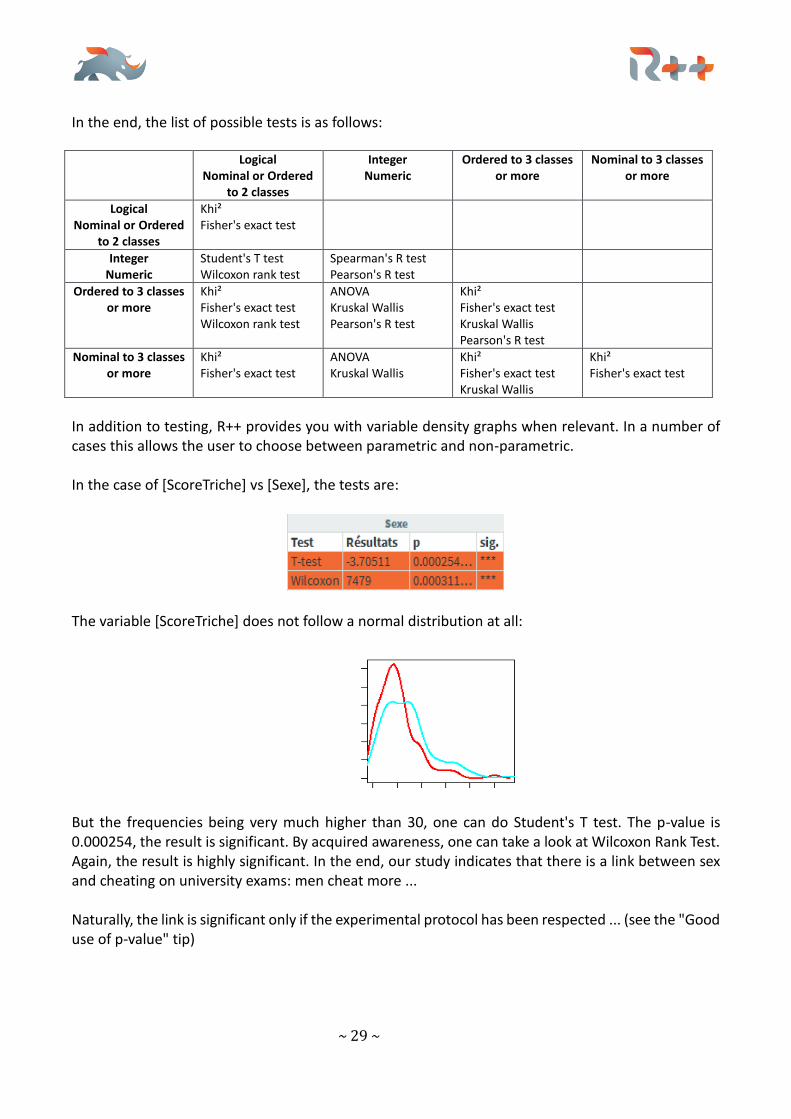
In addition to testing, R++ provides you with variable density graphs when relevant. In a number of cases this allows the user to choose between parametric and non-parametric. In the case of [ScoreTriche] vs [Sexe], the tests are:

The variable [ScoreTriche] does not follow a normal distribution at all:

But the frequencies being very much higher than 30, one can do Student's T test. The p-value is 0.000254, the result is significant. By acquired awareness, one can take a look at Wilcoxon Rank Test. Again, the result is highly significant. In the end, our study indicates that there is a link between sex and cheating on university exams: men cheat more ... Naturally, the link is significant only if the experimental protocol has been respected ... (see the "Good use of p-value" tip)

~ 30 ~

VI. Linear regression, logistic regression and ANOVA In the R++ interface, you can perform linear, logistic and ANOVA regressions with simple Drag & Drop.

— A linear regression is calculated to explain a numeric or integer variable, thanks to a model. — A MANOVA does the same thing, the differences between the two being more historical than

mathematical. — A logistic regression models a binary variable (or nominal with two classes).

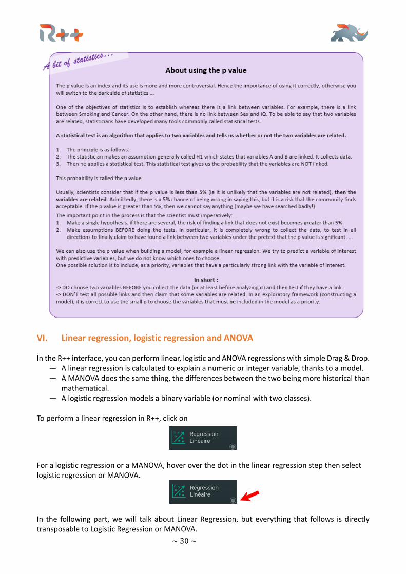
To perform a linear regression in R++, click on

For a logistic regression or a MANOVA, hover over the dot in the linear regression step then select logistic regression or MANOVA.

In the following part, we will talk about Linear Regression, but everything that follows is directly transposable to Logistic Regression or MANOVA.

~ 31 ~

6.1 How to select the variables When you get to the Linear Regression step, R++ asks you to choose the database you want to work on. In this example, click on dn1. The list of dn1 variables will appear on the left part of the window. - The first step in the regression is to choose the "variable to explain" (or variable of interest, or even dependent variable). To do so, just click on it. In our case, we are trying to understand university fraud. Click on ScoreTriche. In the left side of the screen, the ScoreTriche variable is

highlighted in orange . In the right side, it is registered in the "formula" part

. - You can then simply choose the explanatory (or independent) variables by clicking on them on the left. When you select a variable, it is highlighted in blue. This allows you to easily see the variables that are already in the model. In the right part, the model is built as the variables are added. Conversely, you can delete a variable from the model by clicking on its name on the left. In this example, the reasons for the fraud could be due to gender, age and UFR. Click on Sexe, Age and UFR. With each click, the variable is added to the model and the model is updated in real time.

6.2 Automated selection When you have a lot of explanatory variables, it can be difficult to choose the right ones. Statisticians have developed automatic methods that allow us to choose for us. These methods are not perfect, but they do help. ➢ The "Step-by-Step forward" selection method involves adding the variable that best improves

the model, then iterating until no addition improves the model. ➢ The "Step-by-Step backward" selection method consists of deleting the variable, whose de-

letion improves the model the most, then iterating until no further deletions improve the model.

➢ The "mixed Step-by-Step" method consists in each step of adding or removing a variable, depending on what is optimal for the model, then iterating until no addition or deletion im-proves the model.

To help you build your model, R++ has the following methods:

performs a Forward step, that is, it adds the variable that best improves your model. If nothing happens when you click Forward, then your model is already optimal relative to the Forward method.

performs a Backward step, that is, it removes the variable whose removal best improves your model. If nothing happens when you click Backward, then your model is already optimal relative to the Backward method.

allows a complete selection in mixed. R++ stops when the best model is found for the mixed method.

~ 32 ~

Note: The first two options only perform one step, whereas the third one takes as many steps as necessary to find an optimal model. When a statistician builds a model, he wants certain variables to be in his model. If we work on success at school, we want to include the mother's level of education, because, as all specialists are aware, the mother's level of education has a very strong influence on success (much more than the father's education level or household income for example). A model about people’s success that does not contain their mother's education variable would not be taken seriously. A study on wages must necessarily take gender into account. In a cancer study, it is mandatory that the smoking variable be in the model. And so on. Conversely, we may want to prohibit some variables: for example an unreliable variable which would have been very poorly measured; or a variable with a lot of missing values; or a variable very strongly correlated with the variable to be explained. So when the statistician tries to make a model, he/she defines the imposed variables and the forbidden variables. Then he uses automatic techniques such as Step-by-step. R++ allows you to impose or prohibit a variable. To impose a variable, select it (left click, normal). It is highlighted in blue. To ban a variable, right-click on it. It is highlighted in black. This means that automatic methods will not be able to include it in their model.

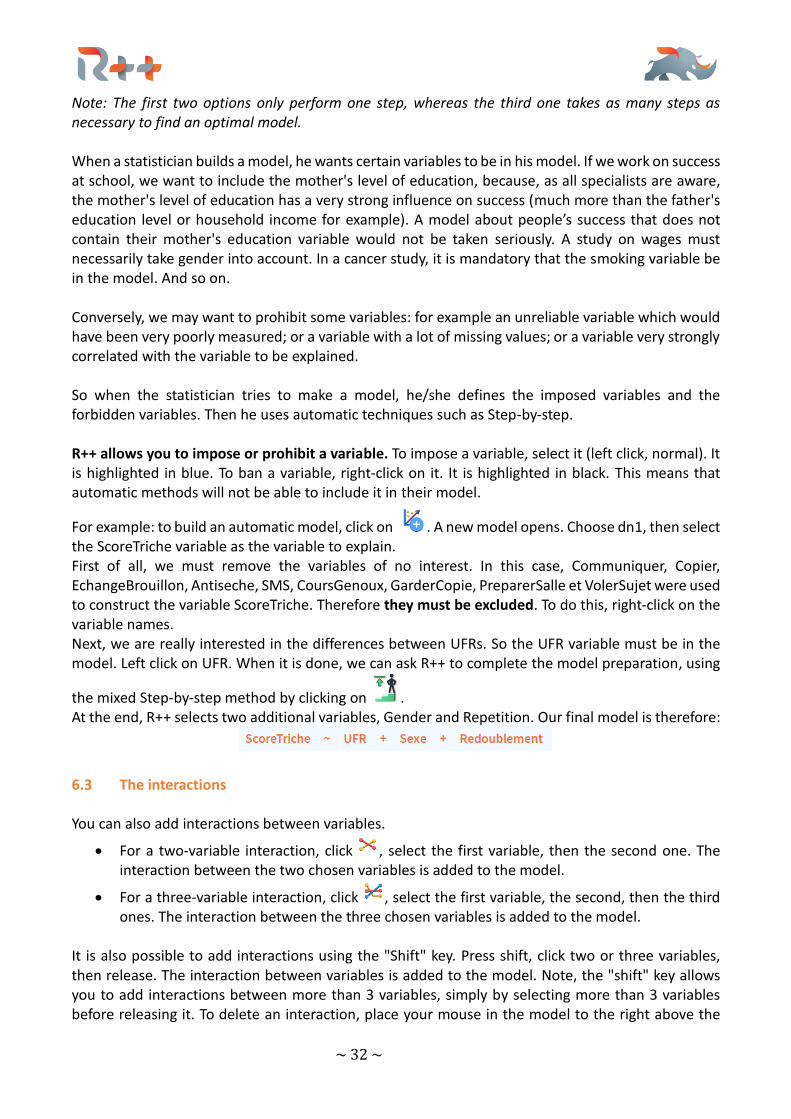
For example: to build an automatic model, click on . A new model opens. Choose dn1, then select the ScoreTriche variable as the variable to explain. First of all, we must remove the variables of no interest. In this case, Communiquer, Copier, EchangeBrouillon, Antiseche, SMS, CoursGenoux, GarderCopie, PreparerSalle et VolerSujet were used to construct the variable ScoreTriche. Therefore they must be excluded. To do this, right-click on the variable names. Next, we are really interested in the differences between UFRs. So the UFR variable must be in the model. Left click on UFR. When it is done, we can ask R++ to complete the model preparation, using

the mixed Step-by-step method by clicking on . At the end, R++ selects two additional variables, Gender and Repetition. Our final model is therefore:

6.3 The interactions You can also add interactions between variables.

• For a two-variable interaction, click , select the first variable, then the second one. The interaction between the two chosen variables is added to the model.

• For a three-variable interaction, click , select the first variable, the second, then the third ones. The interaction between the three chosen variables is added to the model.

It is also possible to add interactions using the "Shift" key. Press shift, click two or three variables, then release. The interaction between variables is added to the model. Note, the "shift" key allows you to add interactions between more than 3 variables, simply by selecting more than 3 variables before releasing it. To delete an interaction, place your mouse in the model to the right above the

~ 33 ~

interaction. A small cross appears: . Clicking on it will remove the interaction.

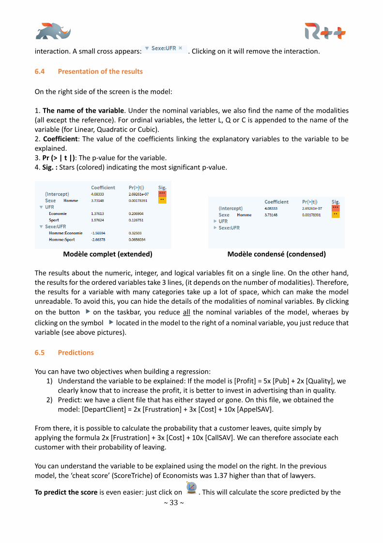
6.4 Presentation of the results

On the right side of the screen is the model: 1. The name of the variable. Under the nominal variables, we also find the name of the modalities (all except the reference). For ordinal variables, the letter L, Q or C is appended to the name of the variable (for Linear, Quadratic or Cubic). 2. Coefficient: The value of the coefficients linking the explanatory variables to the variable to be explained. 3. Pr (> | t |): The p-value for the variable. 4. Sig. : Stars (colored) indicating the most significant p-value.

Modèle complet (extended) Modèle condensé (condensed) The results about the numeric, integer, and logical variables fit on a single line. On the other hand, the results for the ordered variables take 3 lines, (it depends on the number of modalities). Therefore, the results for a variable with many categories take up a lot of space, which can make the model unreadable. To avoid this, you can hide the details of the modalities of nominal variables. By clicking

on the button on the taskbar, you reduce all the nominal variables of the model, wheraes by

clicking on the symbol located in the model to the right of a nominal variable, you just reduce that variable (see above pictures).

6.5 Predictions You can have two objectives when building a regression:

1) Understand the variable to be explained: If the model is [Profit] = 5x [Pub] + 2x [Quality], we clearly know that to increase the profit, it is better to invest in advertising than in quality.

2) Predict: we have a client file that has either stayed or gone. On this file, we obtained the model: [DepartClient] = 2x [Frustration] + 3x [Cost] + 10x [AppelSAV].

From there, it is possible to calculate the probability that a customer leaves, quite simply by applying the formula 2x [Frustration] + 3x [Cost] + 10x [CallSAV]. We can therefore associate each customer with their probability of leaving. You can understand the variable to be explained using the model on the right. In the previous model, the ‘cheat score’ (ScoreTriche) of Economists was 1.37 higher than that of lawyers.

To predict the score is even easier: just click on . This will calculate the score predicted by the

~ 34 ~

model for all variables, then a column with the predicted scores will be added to the data.frame. Then R++ switches to the Data Management step and displays this new added column.

6.6 Finalising a model with large databases

For large databases, linear regression is a particularly time-consuming operation that requires a lot of computing power. In this type of case, in order to keep its interactivity, R++ works on a sample. This allows you to try out different models and display the results in real time (because in most cases, a regression on a random sample will give roughly the same result as a regression on the entire population).

When R++ is working on a sample, the symbol appears. If you want R++ to compute the model on the entire database (when after much testing you are happy with your model), just click on it. The model is re-calculated over the entire database.

Note, when R++ works on the complete database, the calculator is grayed out:

6.7 Saving a model Building a model is often done through testing: trying, getting it wrong, re-trying, still not right, re-trying, etc. We look for a model, we improve it, we go back ... We fumble a bit. All the experts will tell you, sometimes we find a model, but we think we will find better. At the end of the day, it turns out, no, we haven't found anything better. But then… big problem: we no longer remember the exact list of variables which created the best model! We have lost the model that we spent so long finding… To avoid this, R++ has a backup system: when you find a model that seems interesting to you, you

can simply add it to the filmstrip (la ‘pellicule’) by clicking on . If you modify your model, an * appears behind its name to indicate that this model being edited is

not saved: . If you save it again ( ), a window will open. You can save it in the same place (and overwrite the previous version), or give it a new name, in which case it will go to a different cellar box.

VII Exporting

7.1 Editing graphs

Exporting graphs is quite intuitive. At the bottom of the screen, you can choose a graph from the

filmstrip , from all those that were added to the filmstrip during the session. The graph window (central, in blue) shows the graph. In Graph Settings (left in purple) is the list of everything that is editable, in the form of a tree. If you choose a field, the corresponding options are in the Detail window (on the right, in yellow). Some examples of what is modifiable:

• For any given data set, you can choose different types of graphs. For example, a numeric variable can be represented by a histogram or a boxplot. You can change the representation

~ 35 ~

by going to General Type of Graph. But be careful, among all possible types of graph, some may not be relevant. For example, for a numeric variable representing an evolution in time,

the representation will be perfect. On the other hand, for a numeric variable representing sizes of independent individuals, this representation would not make much sense. R++ does not yet know if a representation is relevant or not, it is up to the statistician to decide, for now!

• Sheet parameters (size, margins, background color, but also print settings such as alpha channel and DPI) are available in General Sheet.

• Title, subtitle, X and Y labels are editable via Text. At each step you can change the font, color, size, position and the attributes Bold, Italic and Underlining.

• The Axes, unsurprisingly, make it possible to work on the Axes: limits, graduations, type of lines used and, in some cases, using a logarithmic scale.

• Finally, the general aspect includes everything that is specific to each graph: you may find there, depending on the graph, colors, lines, points, gaps between bars in barplots, widths of boxplots, the number of breaks in histograms, the shapes of densities, stroke styles ...

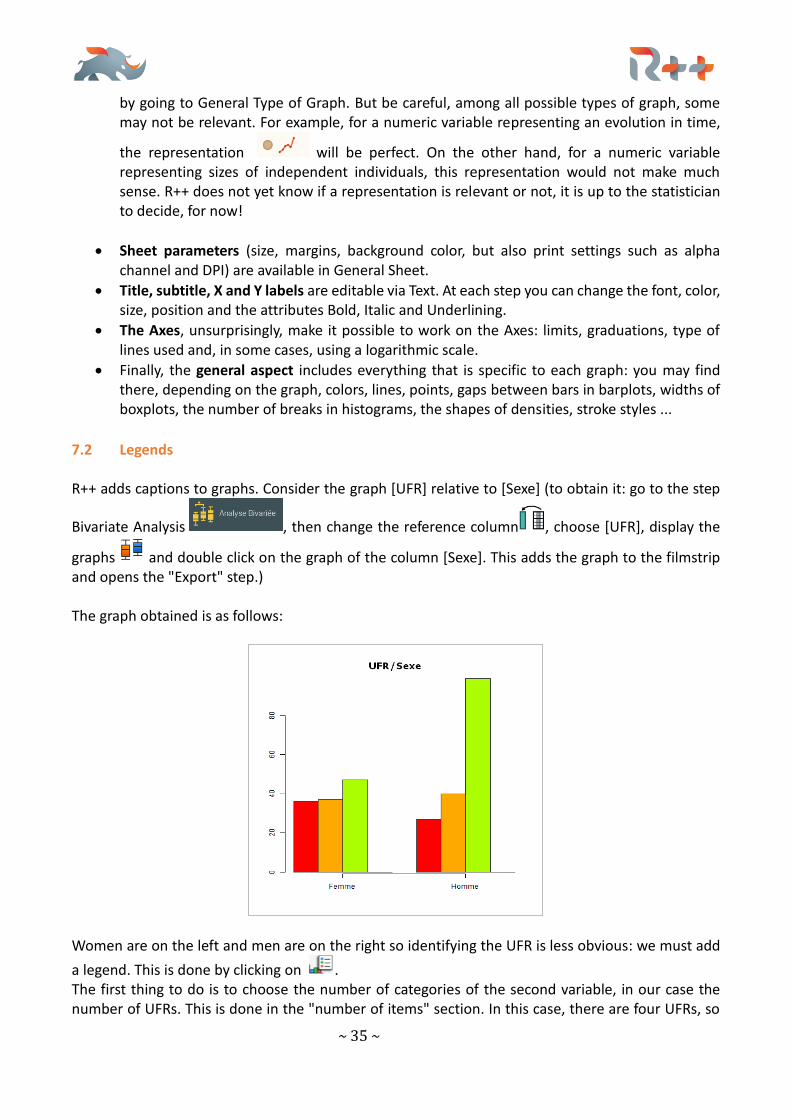
7.2 Legends R++ adds captions to graphs. Consider the graph [UFR] relative to [Sexe] (to obtain it: go to the step

Bivariate Analysis , then change the reference column , choose [UFR], display the

graphs and double click on the graph of the column [Sexe]. This adds the graph to the filmstrip and opens the "Export" step.) The graph obtained is as follows:

Women are on the left and men are on the right so identifying the UFR is less obvious: we must add

a legend. This is done by clicking on . The first thing to do is to choose the number of categories of the second variable, in our case the number of UFRs. This is done in the "number of items" section. In this case, there are four UFRs, so

~ 36 ~

we must add two by clicking on . Then we change the default names in Law, Economy, Sport and Language. The second step is about choosing the type of legend. You can either work with lines and dots, or with

fill textures. For a bivariate barplot, fill texture seems more appropriate. Click on . You can choose a single color for all the boxes, but in this example, we want to differentiate them. For that, we click on . We can then choose the colors one by one by clicking on the color box. A box displaying the color palette opens. You can then click "Choose a screen color" and a color picker opens.

The easiest way is to click on "Pick Screen Color" and then click directly on the corresponding column. Finally, we can change the position of the legend (it is hiding the bar for Men's Sport), by going to

"Size and Position". You can either use a predefined position or a custom position like .

VIII R scripts

8.1 Overall presentation

As we have just seen, R++ can display statistics semi-automatically via the interface. To go further, R++ also has a "Scripts" step.

This step makes it possible to use the statistical language R and to inherit all its diversity. In particular, it is possible to install R packages. In concrete terms, the Scripts interface consists of two windows: a script editor (in blue) and a console (in red). The script editor allows you to write command lines. And through the console you run them. For example, during the Bivariate step, we may find that those who practice Sport cheat more than those who study Law, and that Men cheat more than Woman. But in Staps, there are a lot more men than women. We therefore want to study the impact of [Sexe] on [ScoreTriche] with adjustment on [UFR]. The R command is:

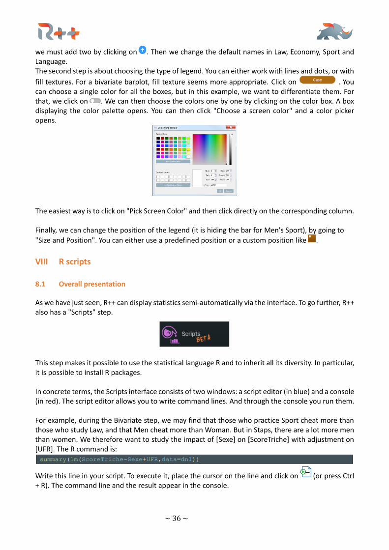
Write this line in your script. To execute it, place the cursor on the line and click on (or press Ctrl + R). The command line and the result appear in the console.

~ 37 ~

The command line is black. If all went well, the result should be blue. If there was an error, it is shown in red. If it's a warning, it'll be in orange. For example, if I forget the "R" of "UFR" in the previous example, I get:

Statistically speaking, we get confirmation, men do cheat more, even after adjusting the UFR column. Note that at each instruction, R++ always displays a little something. This is one of the principles of Human-Computer Interaction: "When it doesn't work, we'll tell you; when it does work, we'll also tell you.” For example, on the instruction a<- 3 the console displays a small Ok (whereas in R, this instruction does not result in a display):

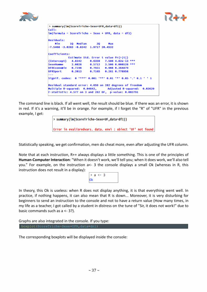
In theory, this Ok is useless: when R does not display anything, it is that everything went well. In practice, if nothing happens, it can also mean that R is down... Moreover, it is very disturbing for beginners to send an instruction to the console and not to have a return value (How many times, in my life as a teacher, I got called by a student in distress on the tune of "Sir, it does not work!" due to basic commands such as a <- 3?). Graphs are also integrated in the console. If you type:

The corresponding boxplots will be displayed inside the console:

~ 38 ~

You can choose to hide them by clicking on .

If you want to work on the graph, you can simply make the filmstrip appear by clicking on , then drag & drop the graph into the filmstrip. You can also double click on the graph, adding it to the filmstrip and opening it at the "Export" step.

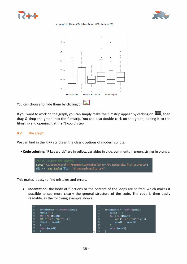
8.2 The script We can find in the R ++ scripts all the classic options of modern scripts: • Code coloring: "R key words" are in yellow, variables in blue, comments in green, strings in orange.

This makes it easy to find mistakes and errors.

• Indentation: the body of functions or the content of the loops are shifted, which makes it possible to see more clearly the general structure of the code. The code is then easily readable, as the following example shows:

~ 39 ~

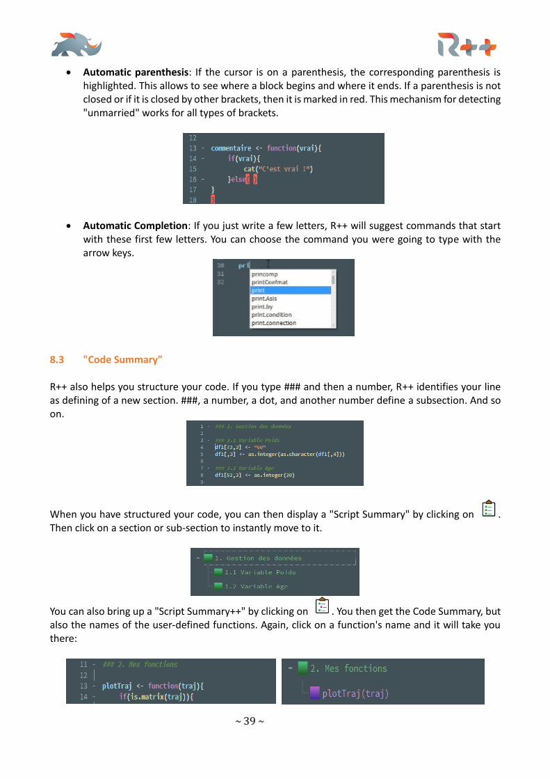
• Automatic parenthesis: If the cursor is on a parenthesis, the corresponding parenthesis is highlighted. This allows to see where a block begins and where it ends. If a parenthesis is not closed or if it is closed by other brackets, then it is marked in red. This mechanism for detecting "unmarried" works for all types of brackets.

• Automatic Completion: If you just write a few letters, R++ will suggest commands that start with these first few letters. You can choose the command you were going to type with the arrow keys.

8.3 "Code Summary" R++ also helps you structure your code. If you type ### and then a number, R++ identifies your line as defining of a new section. ###, a number, a dot, and another number define a subsection. And so on.

When you have structured your code, you can then display a "Script Summary" by clicking on . Then click on a section or sub-section to instantly move to it.

You can also bring up a "Script Summary++" by clicking on . You then get the Code Summary, but also the names of the user-defined functions. Again, click on a function's name and it will take you there:

~ 40 ~

* * * * *