Embed Size (px)
Citation preview
RACE 615 Introduction to Medical Statistics
Sample size for Estimation
Assoc.Prof.Dr.Ammarin Thakkinstian [email protected] www.ceb-rama.org
Doctor of Philosophy Program in Clinical Epidemiology, Section for Clinical Epidemiology & Biostatistics Faculty of Medicine Ramathibodi Hospital, Mahidol University
Semester 1, 2015
2
CONTENTS
INTRODUCTION ...............................................................................................................................6
SAMPLE SIZE FOR ESTIMATION ................................................................................................7
One proportion ...............................................................................................................................7
Diagnostic study ...........................................................................................................................11
SAMPLE SIZE FOR TEST FOR DIFFERENCE ..........................................................................12
One proportion .............................................................................................................................12
Two proportions with independent samples .................................................................................16
Two proportions with dependent samples ....................................................................................29
More than two groups of proportions ...........................................................................................33
Two independent means ...............................................................................................................36
Two dependent means ..................................................................................................................39
More than two groups of means ...................................................................................................42
TEST FOR EQUIVALENCE ...........................................................................................................45
Continuous data ............................................................................................................................45
Two independent means ...............................................................................................................48
Two dependent samples ...............................................................................................................52
Cross – over trial ..........................................................................................................................52
NON – INFERIORITY ....................................................................................................................55
Continuous data ............................................................................................................................55
Two independent means ...............................................................................................................57
Cross-over design .........................................................................................................................59
Dichotomous data ........................................................................................................................61
ASSIGNMENT VI ..............................................................................................................................65
3
OBJECTIVES
Students should be able to:
1. Realize and concern how important a prior sample size estimation is
2. Know what information and background knowledge are required prior to use for
estimating sample size
3. Appropriately estimate sample size corresponding to the primary objective and study
design which aims to:
a. Estimate prevalence (or incidence)
b. Test for differences
c. Test for equivalence or non-inferiority
REFERENCES
1. Kish L. Survey Sampling. New York: John Wiley & Sons, Inc.; 1965.
2. Ingsathit A, Thakkinstian A, Chaiprasert A, et al. Prevalence and risk factors of
chronic kidney disease in the Thai adult population: Thai SEEK study. Nephrology,
dialysis, transplantation : official publication of the European Dialysis and
Transplant Association - European Renal Association. 2010;25(5):1567-1575.
3. Anothaisintawee T, Rattanasiri S, Ingsathit A, et al. Prevalence of chronic kidney
disease: a systematic review and meta-analysis. Clinical nephrology. 2009;71(3):244-
254.
4. Julious SA, Campbell MJ. Tutorial in biostatistics: sample sizes for parallel group
clinical trials with binary data. Statistics in medicine. 2012;31(24):2904-2936.
5. Dupont WD, Plummer WD. Power and Sample Size Calculations: A Review and
Computer Program Controlled Clinical Trials. 1990;11 116-128
4
6. Dupont WD. Power calculations for matched case-control studies. Biometrics.
1988;44(4):1157-1168.
7. Sample size. In: Schlesselman JJ, ed. Case-control studies: Design, conduct, analysis.
Oxford: Oxford University press, 1982:144-165.
8. Barthel FMS, Royston P, Babiker A. Menu-driven facility for complex sample size
calculation in randomized controlled trials with survival or a binary outcome: Update.
STATA Journal. 2005;5(1):123-129.
9. Kamanamool N, McEvoy M, Attia J, et al. Efficacy and adverse events of
mycophenolate mofetil versus cyclophosphamide for induction therapy of lupus
nephritis: systematic review and meta-analysis. Medicine. 2010;89(4):227-235.
10. Bruin J. newtest: command to compute new test. UCLA:
Statistical Consulting Group. 2006. (http://www.ats.ucla.edu/stat/stata/ado/analysis/).
(Accessed 04/09 2013).
11. Julious SA. Sample sizes for clinical trials with normal data. Statistics in medicine.
2004;23(12):1921-1986.
12. Julious SA. SampSize. In: White R, Wroblewski D, Julious SA, et al., eds. Sheffield,
UK: EpiGenesys, 2012.
13. D'Agostino RB, Sr., Massaro JM, Sullivan LM. Non-inferiority trials: design concepts
and issues - the encounters of academic consultants in statistics. Statistics in medicine.
2003;22(2):169-186.
14. Dann RS, Koch GG. Methods for one-sided testing of the difference between
proportions and sample size considerations related to non-inferiority clinical trials.
Pharmaceutical statistics. 2008;7(2):130-141.
5
READING SECTION
Appendix I: Schulz KF, Grimes DA. Sample size calculations in randomised trials:
mandatory and mystical. Lancet. 2005 Apr 9-15;365(9467):1348-53.
Appendix II: Dupont WD. Power calculations for matched case-control studies.
Biometrics.1988 Dec;44(4):1157-68.
Appendix III: Julious SA. Sample sizes for clinical trials with normal data. Stat Med.
2004 Jun 30;23(12):1921-86.
Appendix IV: Julious SA, Campbell MJ. Tutorial in biostatistics: sample sizes for
parallel group clinical trials with binary data. Statistics in medicine
2012;31(24):2904-36.
FURTHER READING
Appendix V: Stat Med. 2002 Oct 15;21(19):2807-14.
Appendix VI: JAMA 2006; 295: 1152
Appendix VII: Statistics in Medicine 2003; 22: 169
Appendix VIII: Pharmaceut Statist 2008; 7: 130
ASSIGNMENT VI (25%)
P. 65, Due: October 15, 2015
6
INTRODUCTION
Sample size estimation is a requirement that investigators need to plan before conducting
research. Methods of estimation should be clearly described in the research proposal. Why do
we need to estimate sample size is a common question that investigators usually ask. The
reasons behind this are as follows: It will lead investigators to have ideas how big or small
effect size which the study will be able to detect at the end given the estimated sample size.
Once the sample size is estimated, it will aid investigators to assess feasibility considering time
required, estimated budget, magnitude of interested event, and manpower that are required for
conducting that research.
Before estimating sample size, statistician and investigator need to clarify themselves for:
- What are the primary/secondary objectives,
- What is the study design,
- Will the sample size be estimated based on the primary objective only, or it will be
covered both primary and secondary objectives?
- What information do we require for estimation and where/how to obtain?
For instance we may need: prevalence/incidence of interested disease, expected
numbers of patients/month/year in each setting, effect size that investigators want to
determine, etc.
- How to set up these values
- Type I (or false positive) and II errors (or false negative)
- Size of difference (or equivalence) that the investigator wants
to detect. This should be discussed within the research team
how big/small the difference needs to be for clinical
significance.
This module describes how to estimate sample size in health science research, which primarily
aims for estimation and hypothesis testing. For hypothesis testing, tests for difference and
equivalence/non-inferiority are covered for both continuous and dichotomous outcomes.
7
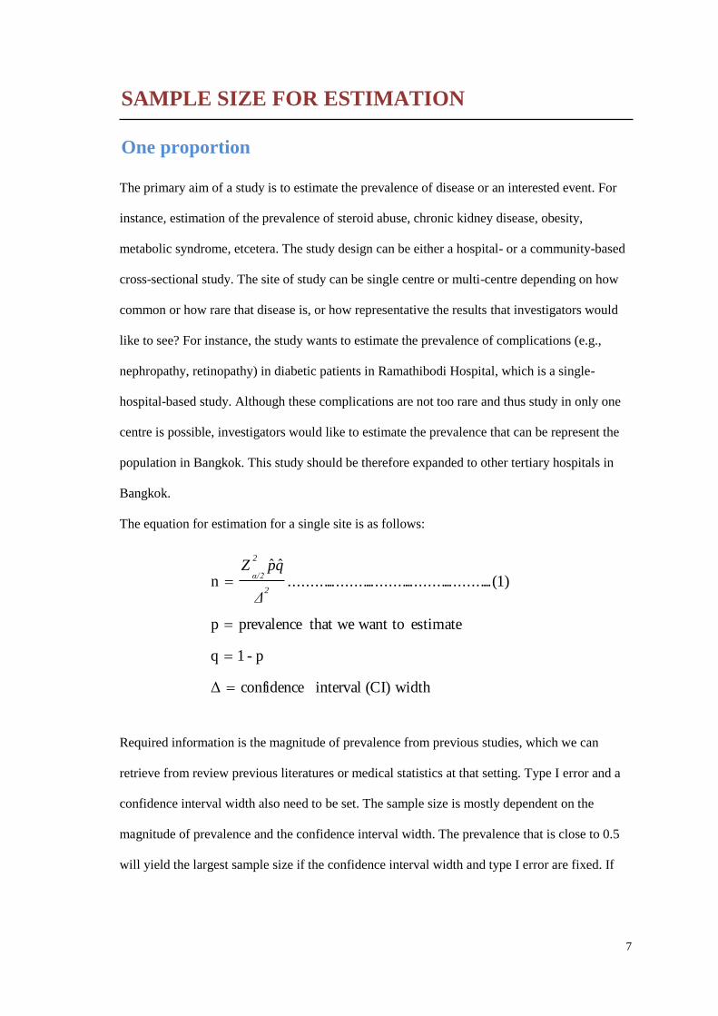
SAMPLE SIZE FOR ESTIMATION
One proportion
The primary aim of a study is to estimate the prevalence of disease or an interested event. For
instance, estimation of the prevalence of steroid abuse, chronic kidney disease, obesity,
metabolic syndrome, etcetera. The study design can be either a hospital- or a community-based
cross-sectional study. The site of study can be single centre or multi-centre depending on how
common or how rare that disease is, or how representative the results that investigators would
like to see? For instance, the study wants to estimate the prevalence of complications (e.g.,
nephropathy, retinopathy) in diabetic patients in Ramathibodi Hospital, which is a single-
hospital-based study. Although these complications are not too rare and thus study in only one
centre is possible, investigators would like to estimate the prevalence that can be represent the
population in Bangkok. This study should be therefore expanded to other tertiary hospitals in
Bangkok.
The equation for estimation for a single site is as follows:
width(CI) interval confidenceΔ
p-1q
estimate want to that weprevalencep
..(1)..................................................ˆˆ
n
2
2
α/2
Δ
qpZ
Required information is the magnitude of prevalence from previous studies, which we can
retrieve from review previous literatures or medical statistics at that setting. Type I error and a
confidence interval width also need to be set. The sample size is mostly dependent on the
magnitude of prevalence and the confidence interval width. The prevalence that is close to 0.5
will yield the largest sample size if the confidence interval width and type I error are fixed. If
8
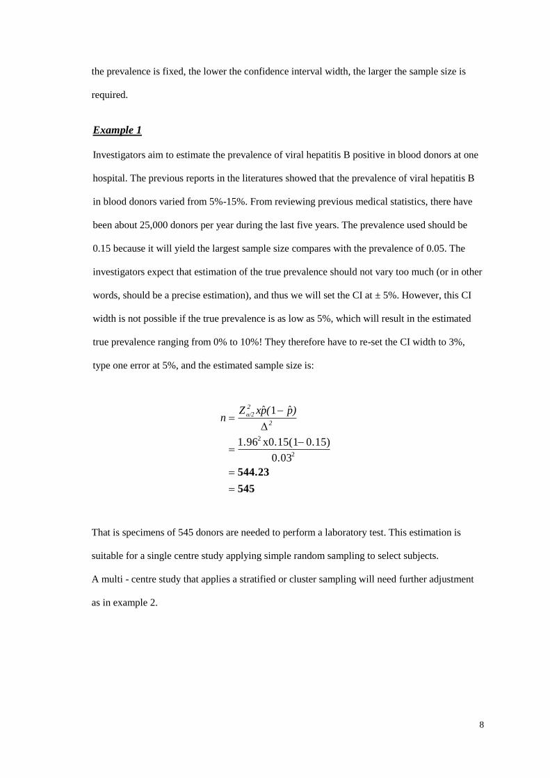
the prevalence is fixed, the lower the confidence interval width, the larger the sample size is
required.
Example 1
Investigators aim to estimate the prevalence of viral hepatitis B positive in blood donors at one
hospital. The previous reports in the literatures showed that the prevalence of viral hepatitis B
in blood donors varied from 5%-15%. From reviewing previous medical statistics, there have
been about 25,000 donors per year during the last five years. The prevalence used should be
0.15 because it will yield the largest sample size compares with the prevalence of 0.05. The
investigators expect that estimation of the true prevalence should not vary too much (or in other
words, should be a precise estimation), and thus we will set the CI at ± 5%. However, this CI
width is not possible if the true prevalence is as low as 5%, which will result in the estimated
true prevalence ranging from 0% to 10%! They therefore have to re-set the CI width to 3%,
type one error at 5%, and the estimated sample size is:
545
544.23
2
2
0.03
0.15)x0.15(11.96
Δ
ˆ1ˆ2
2
α/2 )p(pxZn
That is specimens of 545 donors are needed to perform a laboratory test. This estimation is
suitable for a single centre study applying simple random sampling to select subjects.
A multi - centre study that applies a stratified or cluster sampling will need further adjustment
as in example 2.
9
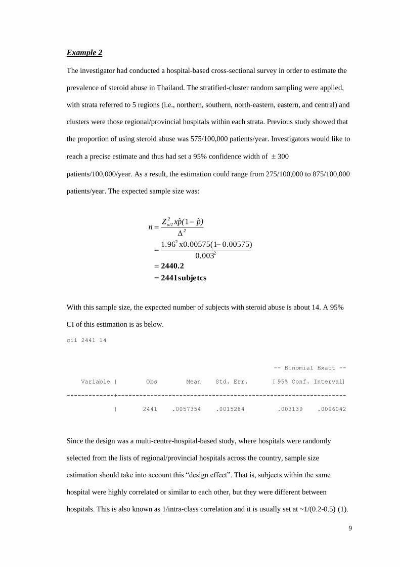
Example 2
The investigator had conducted a hospital-based cross-sectional survey in order to estimate the
prevalence of steroid abuse in Thailand. The stratified-cluster random sampling were applied,
with strata referred to 5 regions (i.e., northern, southern, north-eastern, eastern, and central) and
clusters were those regional/provincial hospitals within each strata. Previous study showed that
the proportion of using steroid abuse was 575/100,000 patients/year. Investigators would like to
reach a precise estimate and thus had set a 95% confidence width of 300
patients/100,000/year. As a result, the estimation could range from 275/100,000 to 875/100,000
patients/year. The expected sample size was:
subjetcs 2441
2440.2
2
2
0.003
0.00575)x0.00575(11.96
Δ
ˆ1ˆ2
2
α/2 )p(pxZn
With this sample size, the expected number of subjects with steroid abuse is about 14. A 95%
CI of this estimation is as below.
cii 2441 14
-- Binomial Exact --
Variable | Obs Mean Std. Err. [95% Conf. Interval]
-------------+---------------------------------------------------------------
| 2441 .0057354 .0015284 .003139 .0096042
Since the design was a multi-centre-hospital-based study, where hospitals were randomly
selected from the lists of regional/provincial hospitals across the country, sample size
estimation should take into account this “design effect”. That is, subjects within the same
hospital were highly correlated or similar to each other, but they were different between
hospitals. This is also known as 1/intra-class correlation and it is usually set at ~1/(0.2-0.5) (1).
10
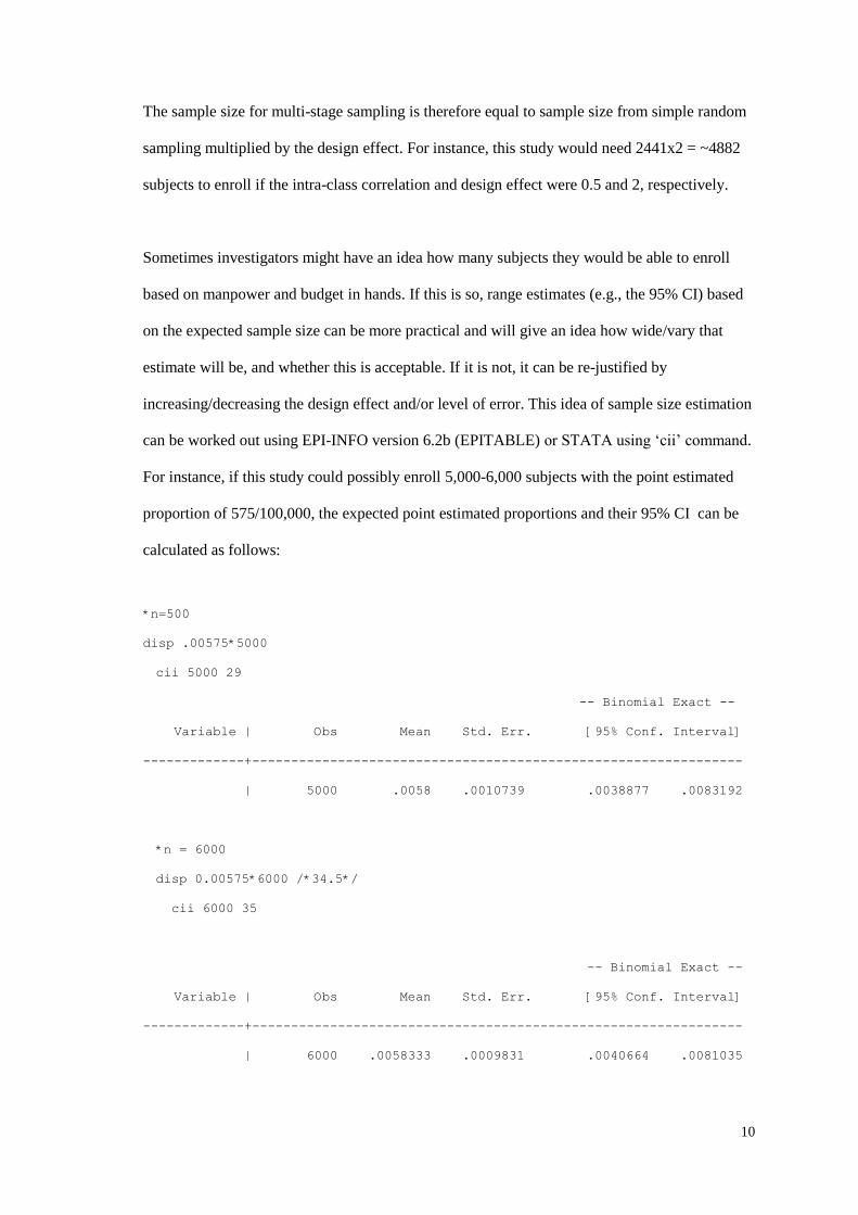
The sample size for multi-stage sampling is therefore equal to sample size from simple random
sampling multiplied by the design effect. For instance, this study would need 2441x2 = ~4882
subjects to enroll if the intra-class correlation and design effect were 0.5 and 2, respectively.
Sometimes investigators might have an idea how many subjects they would be able to enroll
based on manpower and budget in hands. If this is so, range estimates (e.g., the 95% CI) based
on the expected sample size can be more practical and will give an idea how wide/vary that
estimate will be, and whether this is acceptable. If it is not, it can be re-justified by
increasing/decreasing the design effect and/or level of error. This idea of sample size estimation
can be worked out using EPI-INFO version 6.2b (EPITABLE) or STATA using ‘cii’ command.
For instance, if this study could possibly enroll 5,000-6,000 subjects with the point estimated
proportion of 575/100,000, the expected point estimated proportions and their 95% CI can be
calculated as follows:
*n=500
disp .00575*5000
cii 5000 29
-- Binomial Exact --
Variable | Obs Mean Std. Err. [95% Conf. Interval]
-------------+---------------------------------------------------------------
| 5000 .0058 .0010739 .0038877 .0083192
*n = 6000
disp 0.00575*6000 /*34.5*/
cii 6000 35
-- Binomial Exact --
Variable | Obs Mean Std. Err. [95% Conf. Interval]
-------------+---------------------------------------------------------------
| 6000 .0058333 .0009831 .0040664 .0081035
11
Diagnostic study
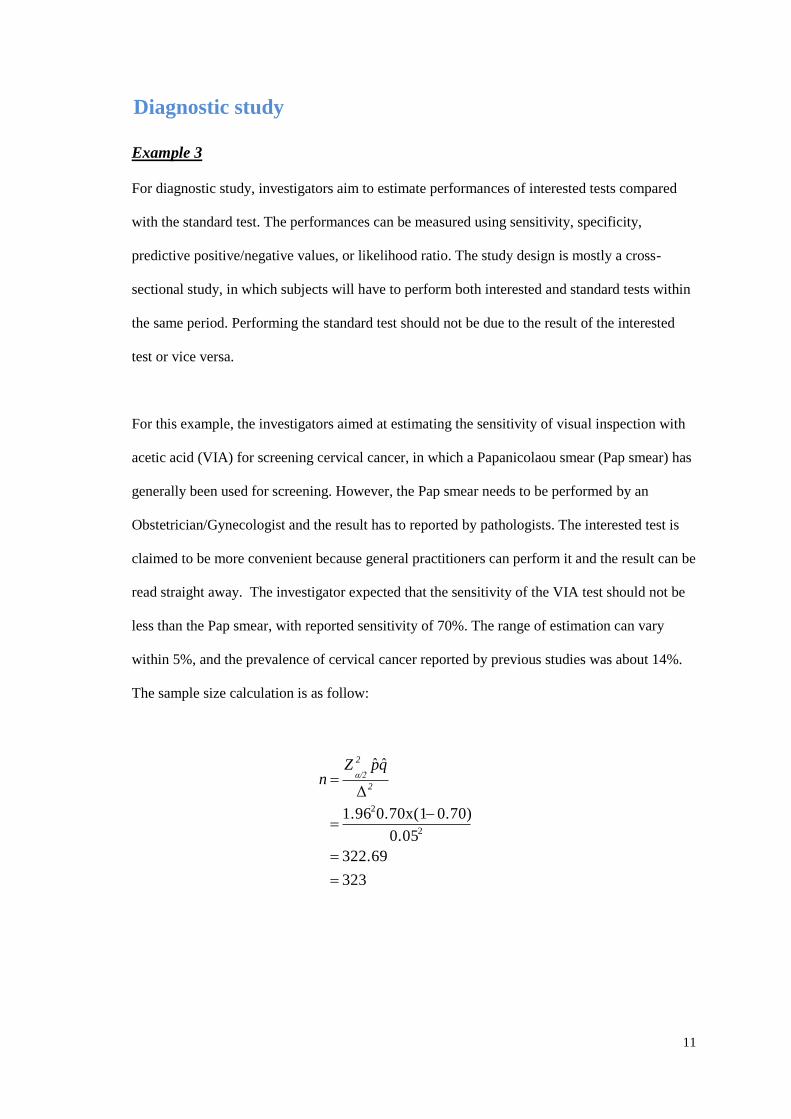
Example 3
For diagnostic study, investigators aim to estimate performances of interested tests compared
with the standard test. The performances can be measured using sensitivity, specificity,
predictive positive/negative values, or likelihood ratio. The study design is mostly a cross-
sectional study, in which subjects will have to perform both interested and standard tests within
the same period. Performing the standard test should not be due to the result of the interested
test or vice versa.
For this example, the investigators aimed at estimating the sensitivity of visual inspection with
acetic acid (VIA) for screening cervical cancer, in which a Papanicolaou smear (Pap smear) has
generally been used for screening. However, the Pap smear needs to be performed by an
Obstetrician/Gynecologist and the result has to reported by pathologists. The interested test is
claimed to be more convenient because general practitioners can perform it and the result can be
read straight away. The investigator expected that the sensitivity of the VIA test should not be
less than the Pap smear, with reported sensitivity of 70%. The range of estimation can vary
within 5%, and the prevalence of cervical cancer reported by previous studies was about 14%.
The sample size calculation is as follow:
323
322.69
0.05
0.70)0.70x(11.96
Δ
ˆˆ
2
2
2
2
α/2qpZ
n
12
That is 323 subjects with cervical cancer are needed in order to estimate the sensitivity which
the investigators expected. As for the prevalence, 323/0.14 = 2307.14 = 2308 subjects are
required to enroll.
SAMPLE SIZE FOR TEST FOR DIFFERENCE
One proportion
We usually compare a studied prevalence with the prevalence in the reference population or the
previous prevalence that has been reported in the literatures. For instance,
- compare prevalence of diabetes in Thailand with the prevalence reported in China,
- compare prevalence of chronic kidney disease in the Thai population with Caucasians
- compare prevalence of Gln and Glu alleles of beta-2 adrenoreceptor polymorphisms
in the Thai population with those studied in Caucasians.
All of these examples have only one group of studied population and most study designs are
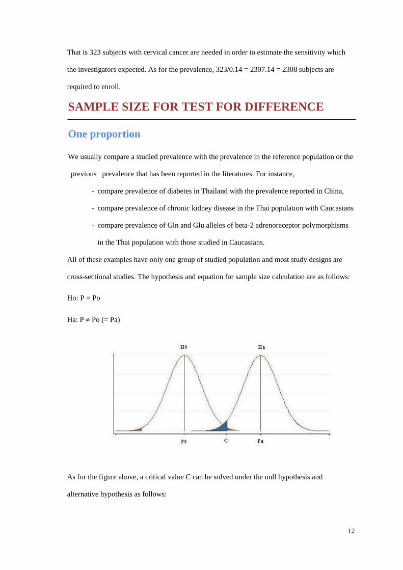
cross-sectional studies. The hypothesis and equation for sample size calculation are as follows:
Ho: P = Po
Ha: P Po (= Pa)
As for the figure above, a critical value C can be solved under the null hypothesis and
alternative hypothesis as follows:
13
2
0
2
β1002/α
00β12/α0
β12/α0
β1
a
0
)(
)1()1(
)1()1(1
)(
)1()1(
)1(
HUnder
1
HUnder
PP
PPZPPZn
PPZPPZn
PP
n
PPZP
n
PPZP
n
PPZPc
n
)P(PZPc
a
aa
aa
aaa
aa
aaa
00α/20
Example 4
Investigators would like to conduct a cross-sectional survey study to primarily estimate the
prevalence of CKD across Thailand (2). Investigators had also asked whether CKD in Thailand
was as common as in other Asian countries. They therefore had a secondary objective as
comparing the CKD prevalence in Thailand to the prevalence in Asian population. From a
systematic review of previous studies, the pooled prevalence of CKD stage III or higher in the
Asian population was 8.3% (95% CI: 4.3%, 12.4%) (3) They wondered how many subjects
were needed to enroll in order to answer the secondary objective. Type I and II errors were
respectively set at 5% and 20%, and size of difference that they wanted to detect was ±5%. The
sample size could be estimated as follows:
14
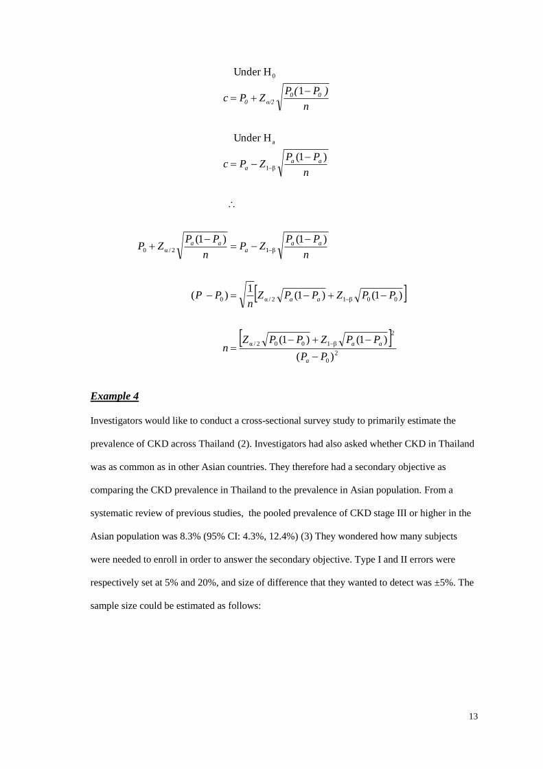
273
9.272
)083.0133.0(
133.01(133.084.0)083.01(083.096.12
2
2
oa
2
aaβooα/2
)P(P
)P(1PZ)P(1PZn
Thus, it was required at least 273 subjects to compare the current vs previous prevalence, if, and
only if, the difference was 5% or higher.
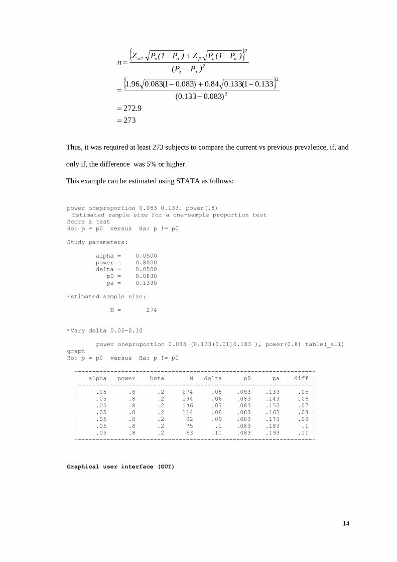
This example can be estimated using STATA as follows:
power oneproportion 0.083 0.133, power(.8)
Estimated sample size for a one-sample proportion test
Score z test
Ho: p = p0 versus Ha: p != p0
Study parameters:
alpha = 0.0500
power = 0.8000
delta = 0.0500
p0 = 0.0830
pa = 0.1330
Estimated sample size:
N = 274
*Vary delta 0.05-0.10
power oneproportion 0.083 (0.133(0.01)0.183 ), power(0.8) table(_all)
graph
Ho: p = p0 versus Ha: p != p0
+-----------------------------------------------------------------+
| alpha power beta N delta p0 pa diff |
|-----------------------------------------------------------------|
| .05 .8 .2 274 .05 .083 .133 .05 |
| .05 .8 .2 194 .06 .083 .143 .06 |
| .05 .8 .2 146 .07 .083 .153 .07 |
| .05 .8 .2 114 .08 .083 .163 .08 |
| .05 .8 .2 92 .09 .083 .173 .09 |
| .05 .8 .2 75 .1 .083 .183 .1 |
| .05 .8 .2 63 .11 .083 .193 .11 |
+-----------------------------------------------------------------+
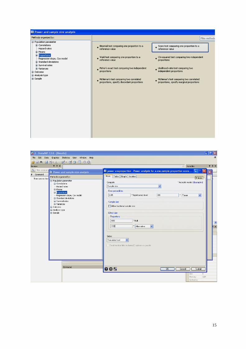
Graphical user interface (GUI)
15
16
Two proportions with independent samples
Clinical trial or observational study sometime aims to compare proportions between two independent
groups. For instance:
- Compare proportions of Glu alleles between asthma and non-asthma groups
- Compare proportions of chronic kidney disease between patients whose
hemoglobin-A1-C < 6.5% and ≥ 6.5%
- Compare incidence of cardiovascular events between patients who do/do not receive
Rosiglitazone.
- Compare incidence of micro- and macro-albuminuria between patients who receive
Angiotensin Converting Enzyme inhibitor (ACEI) and other hypertensive drugs.
- Compare proportion of remission between patients who receive Mycophenolate
Mofetil (MMF) and Cyclophosphamide.
The test for difference can be two-sided test if a direction of difference is not specified, or one-
sided test (called called superiority) if a direction is specified. If the later, evidences are required
to support the expected direction. The null and alternative hypotheses for a two-sided test are as
follows(4):
Ho: P1 - P2 = 0
Ha: P1 – P2 0
Base on H0: P1 - P2 = 0 = P
2112
11
nn if ;n
P)P(
n
)P(P
n
)P(P
)Var(P)Var(P)PVar(P
2
22
1
11
2121
If the ratio of treatment per control group is assigned as 1:1, the equation for sample size
calculation is as follows:
Under the Ho, a critical value C is defined as
17
n
P)2P(Zc α/2
10
Under the Ha, it is defined as
2
PPP
)P(P
)P(P)P(PZP)P(Zn
)P(P)P(PZP)P(Zn
1)P(P
)P(P)P(PZn
1)P(PP)2P(Z
n
1
n
)P(P
n
)P(PZ)P(P
n
P)2P(Z
n
)P(P
n
)P(PZ)P(Pc
21
2
21
2
2211β1α/2
2211β1α/221
2211β121α/2
2
22
1
11
β121α/2
2
22
1
11
β121
1112
1112
111
111
11
The ratio of treatment versus control (n1:n2) can be varied from 1:1. In the case that the new
treatment is quite expensive compared with the standard treatment, or it is more likely to be
harm from side effect/s of the new treatment than the standard one, the investigator may assign
as 1: 2, 1:3, or 1: 4 for the new treatment versus the standard groups. This is also applicable in
an observational case-controlled study in case that the disease is very rare and it is difficult to
achieve equal numbers of cases and controls. An investigator thus designs to have more
controls (say 1:2, 1:3, or even 1:4) than cases. Also the same as in a cohort study where
exposure is rare compared to non-exposure.
Information needs for calculations (e.g., event proportion in control group, size of difference to
be detected, false positive (type I) & negative (type II)) should be set and clearly described in
the proposal. Sources of information should be cited if possible. The false positive and false
negative rates are usually fixed whereas the size of difference that can be detected (P1-P2, also
called size of detectable, or effect size) can be varied and this component mainly determines the
sample size. The smaller the size of detectable, the larger the sample size is. How to set up this
18
effect size is to justify between having clinical significance and feasibility of conducting
research. The size should be as minimal as possible to reach to clinical significance, but
practically sometimes this is not feasible with limitations in time, cost, and manpower.
Discussion with the team will help to get ideas about this size.
The type I error (α) or false positive rate is the error from rejecting the null hypothesis when it
is true (i.e., there is no treatment effect in the population). This error usually is set at 5% or
lower in clinical trials or medical/health research. This means the investigators will face the
false positive of 5% if they reject the (true) null hypothesis.
The type II error (β) or the false negative occurs when the study concludes that there is no
treatment effect, but in fact the treatment effect exists in the population, i.e., the null hypothesis
is false. This is usually set at 0.20 or lower, and thus the power of test (i.e., 1- β) is 80% or
higher; which is the probability of detecting the treatment effect if in fact the treatment effect is
present.
READ more detail in Appendix I
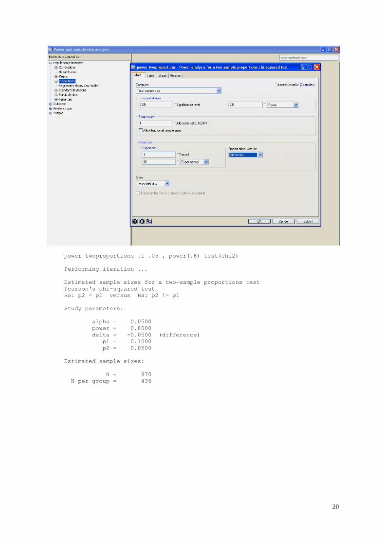
Example 5
Investigators wanted to assess whether receiving calcium supplement 500 mg/day would be
able to reduce osteoporotic fracture compared with receiving placebo. The incidence of fracture
in the general population was 0.1, reducing the incidence to be 0.05 would be clinically
significant. Type I & II errors were set at 5% and 20%, respectively. The sample size
calculation was as follows:

19
434
433.9
0.05)(0.10
0.05)0.05(10.10)0.10(10.840.075)2x0.075(11.96
0.0752
0.050.1
111
2
2
n
2
PPP
)P(P
)P((P)P(PZ)P(P2Zn
21
2
21
2
2211βα/2
They needed at least 434 subjects per group to enroll to the study in order to detect the
difference of fracture rate between groups of 5%. It is common in a follow-up study that
subjects may be lost to follow-up and the sample size should be planned for this regard. If
previous studies of their colleagues in the same settings showed that the lost follow-up rate was
about 20%, therefore the total sample size should be 434+434x0.2 = 521 subjects/group.
This example can be worked out using statistical software such as STATA or PS as follows:
STATA 13: GUI
20
power twoproportions .1 .05 , power(.8) test(chi2)
Performing iteration ...
Estimated sample sizes for a two-sample proportions test
Pearson's chi-squared test
Ho: p2 = p1 versus Ha: p2 != p1
Study parameters:
alpha = 0.0500
power = 0.8000
delta = -0.0500 (difference)
p1 = 0.1000
p2 = 0.0500
Estimated sample sizes:
N = 870
N per group = 435
21
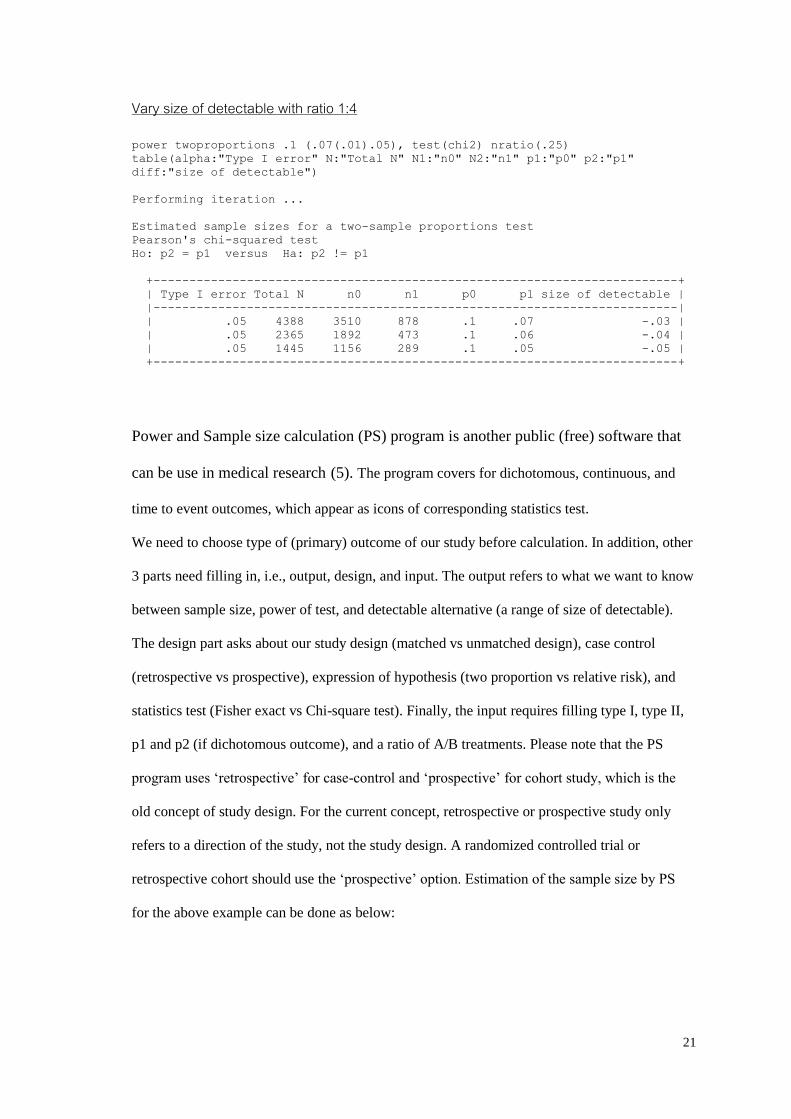
Vary size of detectable with ratio 1:4
power twoproportions .1 (.07(.01).05), test(chi2) nratio(.25)
table(alpha:"Type I error" N:"Total N" N1:"n0" N2:"n1" p1:"p0" p2:"p1"
diff:"size of detectable")
Performing iteration ...
Estimated sample sizes for a two-sample proportions test
Pearson's chi-squared test
Ho: p2 = p1 versus Ha: p2 != p1
+-------------------------------------------------------------------------+
| Type I error Total N n0 n1 p0 p1 size of detectable |
|-------------------------------------------------------------------------|
| .05 4388 3510 878 .1 .07 -.03 |
| .05 2365 1892 473 .1 .06 -.04 |
| .05 1445 1156 289 .1 .05 -.05 |
+-------------------------------------------------------------------------+
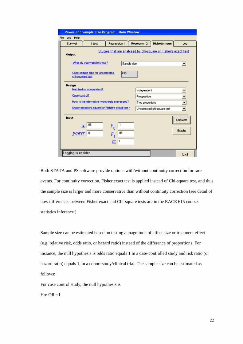
Power and Sample size calculation (PS) program is another public (free) software that
can be use in medical research (5). The program covers for dichotomous, continuous, and
time to event outcomes, which appear as icons of corresponding statistics test.
We need to choose type of (primary) outcome of our study before calculation. In addition, other
3 parts need filling in, i.e., output, design, and input. The output refers to what we want to know
between sample size, power of test, and detectable alternative (a range of size of detectable).
The design part asks about our study design (matched vs unmatched design), case control
(retrospective vs prospective), expression of hypothesis (two proportion vs relative risk), and
statistics test (Fisher exact vs Chi-square test). Finally, the input requires filling type I, type II,
p1 and p2 (if dichotomous outcome), and a ratio of A/B treatments. Please note that the PS
program uses ‘retrospective’ for case-control and ‘prospective’ for cohort study, which is the
old concept of study design. For the current concept, retrospective or prospective study only
refers to a direction of the study, not the study design. A randomized controlled trial or
retrospective cohort should use the ‘prospective’ option. Estimation of the sample size by PS
for the above example can be done as below:
22
Both STATA and PS software provide options with/without continuity correction for rare
events. For continuity correction, Fisher exact test is applied instead of Chi-square test, and thus
the sample size is larger and more conservative than without continuity correction (see detail of
how differences between Fisher exact and Chi-square tests are in the RACE 615 course:
statistics inference.)
Sample size can be estimated based on testing a magnitude of effect size or treatment effect
(e.g. relative risk, odds ratio, or hazard ratio) instead of the difference of proportions. For
instance, the null hypothesis is odds ratio equals 1 in a case-controlled study and risk ratio (or
hazard ratio) equals 1, in a cohort study/clinical trial. The sample size can be estimated as
follows:
For case control study, the null hypothesis is
Ho: OR =1
23
)P(1ORxP
ORxPP
11
12
For cohort or randomized control trial, the null hypothesis is
Ho: RR =1
0
1
I
IRR
Then, estimation of P2 or I1 can be done using the above equations and substituting it in the
equation for 2 proportions, or using STATA for calculation, or using PS with option ‘relative
risk’ for hypothesis expression.
Example 6
In the case-controlled study of risk factors of steroid abuse, investigators wanted to assess
whether using traditional medicine was associated with adrenal insufficiency or adrenal crisis.
Previous reports showed that the prevalence of using traditional medicine in the general
population was about 15%. The odds ratio that can be detected is set at 1.5. Since the case (i.e.,
adrenal insufficiency or adrenal crisis) is quite rare, the ratio of case versus controls is set at 1:4.
False positive and false negative rates are set at 5% and 20%, respectively. The estimated P2 can
be estimated as:
0.21
0.15)(11.5x0.15
1.5x0.15P
)P(1ORxP
ORxPP
2
11
12
24
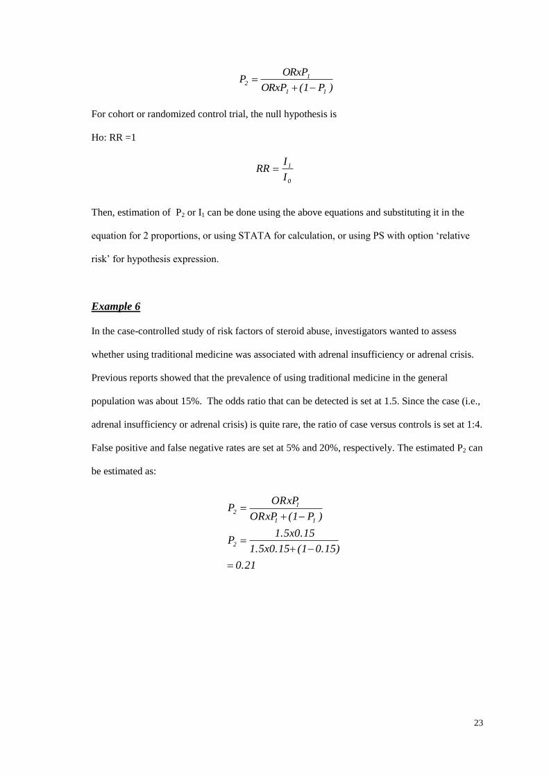
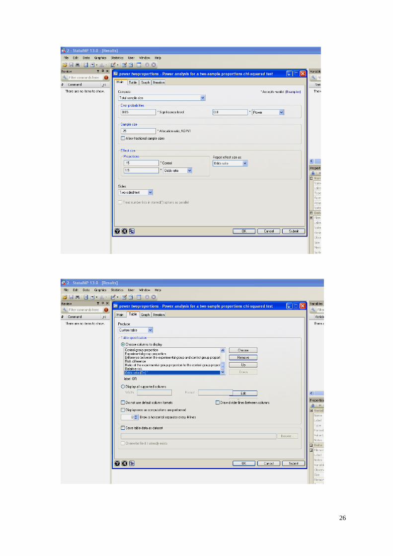
We can use PS to calculate sample size straight away as follows:
This study needs to enroll 397 cases and 397x4 controls to be able to detect the odds ratio of
1.5. There might be incomplete or missing data about 5%, taking this into account will require
2,085 subjects in total.
This can be estimated by STATA 13 as follows:
power twoproportions .15, test(chi2) oratio(1.5) nratio(.25)
table(alpha:"Type I error" power:"Power of test" N:"Total N" N1:"n0" N2:"n1"
delta:"effect size" oratio:"OR")
Performing iteration ...
Estimated sample sizes for a two-sample proportions test
Pearson's chi-squared test
Ho: p2 = p1 versus Ha: p2 != p1

25
+------------------------------------------------------------------------+
| Type I error Power of test Total N n0 n1 effect size OR |
|------------------------------------------------------------------------|
| .05 .8 1984 1587 397 1.5 1.5 |
+------------------------------------------------------------
26
27
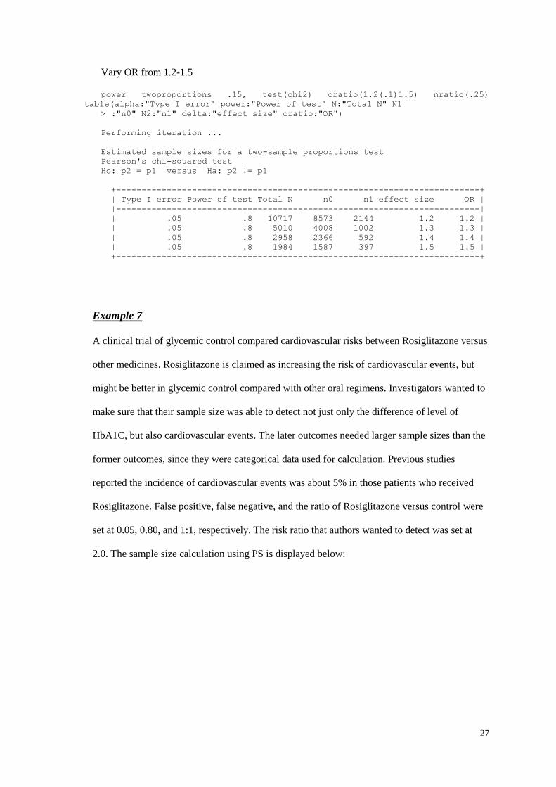
Vary OR from 1.2-1.5
power twoproportions .15, test(chi2) oratio(1.2(.1)1.5) nratio(.25)
table(alpha:"Type I error" power:"Power of test" N:"Total N" N1
> :"n0" N2:"n1" delta:"effect size" oratio:"OR")
Performing iteration ...
Estimated sample sizes for a two-sample proportions test
Pearson's chi-squared test
Ho: p2 = p1 versus Ha: p2 != p1
+------------------------------------------------------------------------+
| Type I error Power of test Total N n0 n1 effect size OR |
|------------------------------------------------------------------------|
| .05 .8 10717 8573 2144 1.2 1.2 |
| .05 .8 5010 4008 1002 1.3 1.3 |
| .05 .8 2958 2366 592 1.4 1.4 |
| .05 .8 1984 1587 397 1.5 1.5 |
+------------------------------------------------------------------------+
Example 7
A clinical trial of glycemic control compared cardiovascular risks between Rosiglitazone versus
other medicines. Rosiglitazone is claimed as increasing the risk of cardiovascular events, but
might be better in glycemic control compared with other oral regimens. Investigators wanted to
make sure that their sample size was able to detect not just only the difference of level of
HbA1C, but also cardiovascular events. The later outcomes needed larger sample sizes than the
former outcomes, since they were categorical data used for calculation. Previous studies
reported the incidence of cardiovascular events was about 5% in those patients who received
Rosiglitazone. False positive, false negative, and the ratio of Rosiglitazone versus control were
set at 0.05, 0.80, and 1:1, respectively. The risk ratio that authors wanted to detect was set at
2.0. The sample size calculation using PS is displayed below:
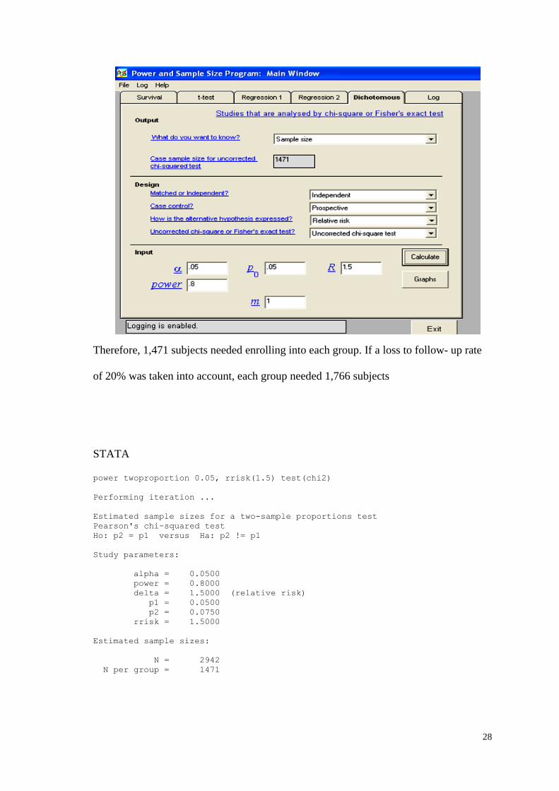
28
Therefore, 1,471 subjects needed enrolling into each group. If a loss to follow- up rate
of 20% was taken into account, each group needed 1,766 subjects
STATA
power twoproportion 0.05, rrisk(1.5) test(chi2)
Performing iteration ...
Estimated sample sizes for a two-sample proportions test
Pearson's chi-squared test
Ho: p2 = p1 versus Ha: p2 != p1
Study parameters:
alpha = 0.0500
power = 0.8000
delta = 1.5000 (relative risk)
p1 = 0.0500
p2 = 0.0750
rrisk = 1.5000
Estimated sample sizes:
N = 2942
N per group = 1471
29
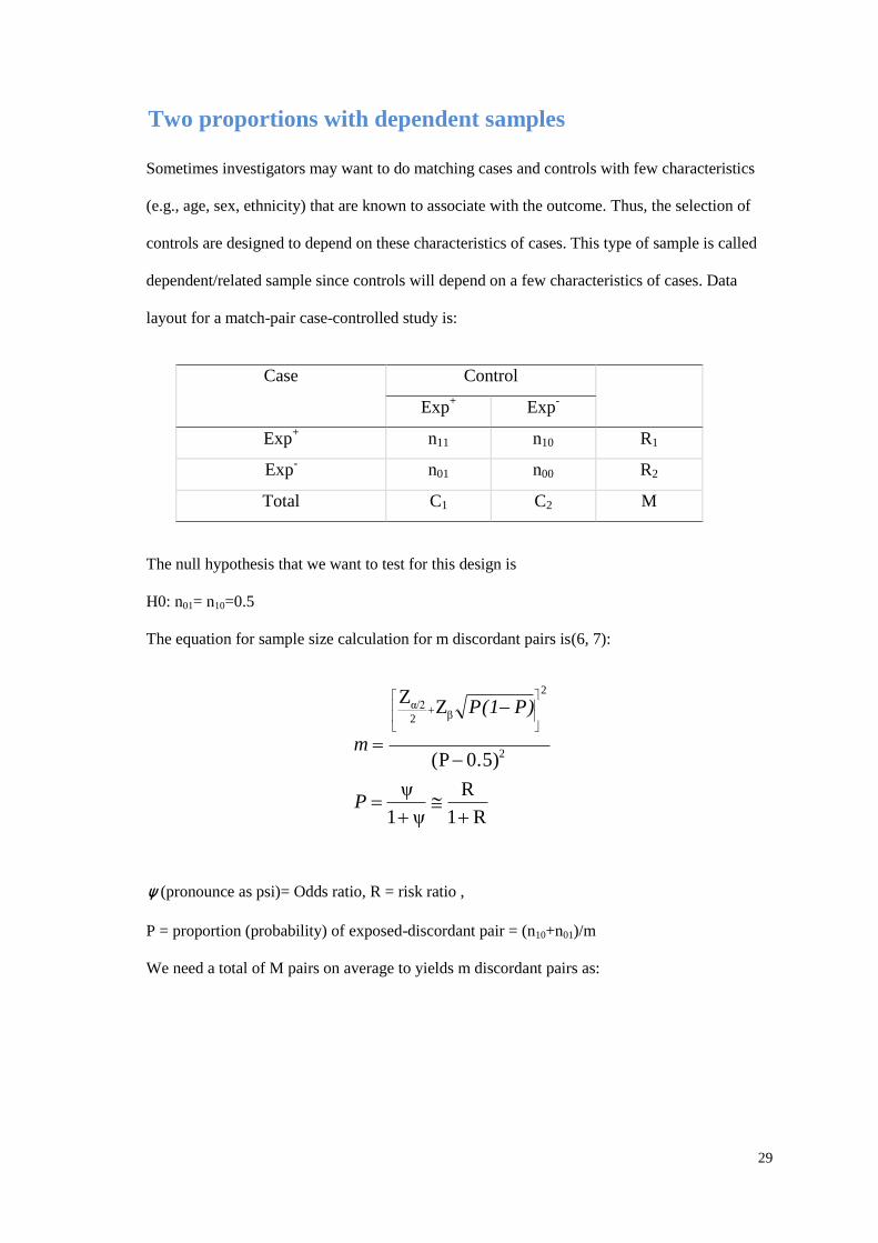
Two proportions with dependent samples
Sometimes investigators may want to do matching cases and controls with few characteristics
(e.g., age, sex, ethnicity) that are known to associate with the outcome. Thus, the selection of
controls are designed to depend on these characteristics of cases. This type of sample is called
dependent/related sample since controls will depend on a few characteristics of cases. Data
layout for a match-pair case-controlled study is:
Case Control
Exp+ Exp
-
Exp+ n11 n10 R1
Exp- n01 n00 R2
Total C1 C2 M
The null hypothesis that we want to test for this design is
H0: n01= n10=0.5
The equation for sample size calculation for m discordant pairs is(6, 7):
R1
R
ψ1
ψ
0.5)(P
ZZ
2
2
β2
α/2
P
P)P(1
m
ψ (pronounce as psi)= Odds ratio, R = risk ratio ,
P = proportion (probability) of exposed-discordant pair = (n10+n01)/m
We need a total of M pairs on average to yields m discordant pairs as:
30
)P(ORxP
ORxPP
qpqpp
p
mM
00
01
0110e
e
1
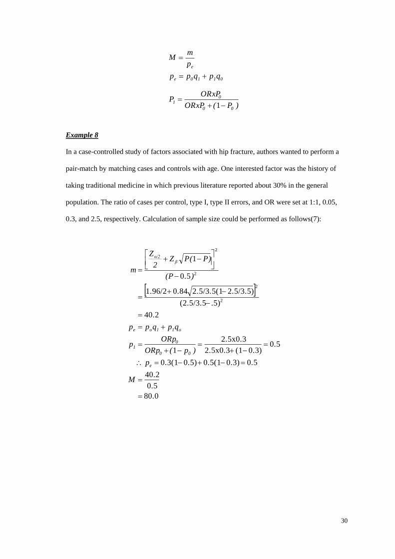
Example 8
In a case-controlled study of factors associated with hip fracture, authors wanted to perform a
pair-match by matching cases and controls with age. One interested factor was the history of
taking traditional medicine in which previous literature reported about 30% in the general
population. The ratio of cases per control, type I, type II errors, and OR were set at 1:1, 0.05,
0.3, and 2.5, respectively. Calculation of sample size could be performed as follows(7):
80.0
0.5
40.2
0.50.3)0.5(10.5)0.3(1
0.50.3)(12.5x0.3
2.5x0.3
1
40.2
.5)(2.5/3.5
2.5/3.5)2.5/3.5(10.841.96/2
0.5
1
2
2
2
2
M
p
)p(ORp
ORpp
qpqpp
)(P
P)P(Z2
Z
m
e
00
01
o11oe
βα/2
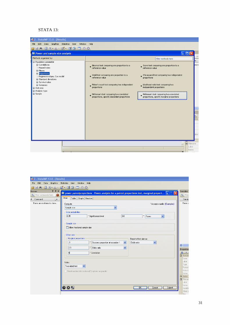
31
STATA 13:
32
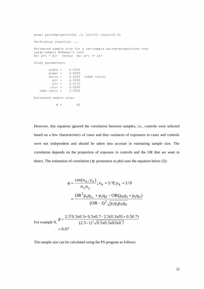
power pairedproportions .3, corr(0) oratio(2.5)
Performing iteration ...
Estimated sample size for a two-sample paired-proportions test
Large-sample McNemar's test
Ho: p+1 = p1+ versus Ha: p+1 != p1+
Study parameters:
alpha = 0.0500
power = 0.8000
delta = 2.5000 (odds ratio)
p1+ = 0.3000
p+1 = 0.5172
corr = 0.0000
odds ratio = 2.5000
Estimated sample size:
N = 82
However, this equation ignored the correlation between samples, i.e., controls were selected
based on a few characteristics of cases and thus variances of exposures in cases and controls
were not independent and should be taken into account in estimating sample size. The
correlation depends on the proportion of exposure in controls and the OR that we want to
detect. The estimation of correlation (φ pronounce as phi) uses the equation below (5):
00112
011001102
kkyx
kk
qpqp)1OR(
)qpqp(ORqpqpOR
0/1y;0/1x;σσ
)y,xcov(φ
For example 8,
0.07
3x0.70.5x0.5x0.1)(2.5
0.50.7)52.5(0.3x0.0.5x0.70.3x0.52.52
2
The sample size can be calculated using the PS program as follows:
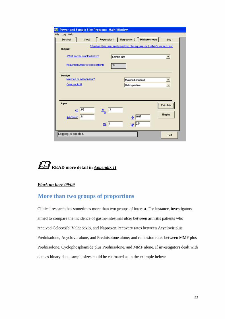
33
READ more detail in Appendix II
Work on here 09/09
More than two groups of proportions
Clinical research has sometimes more than two groups of interest. For instance, investigators
aimed to compare the incidence of gastro-intestinal ulcer between arthritis patients who
received Celecoxib, Valdecoxib, and Naproxen; recovery rates between Acyclovir plus
Prednisolone, Acyclovir alone, and Prednisolone alone; and remission rates between MMF plus
Prednisolone, Cyclophosphamide plus Prednisolone, and MMF alone. If investigators dealt with
data as binary data, sample sizes could be estimated as in the example below:
34
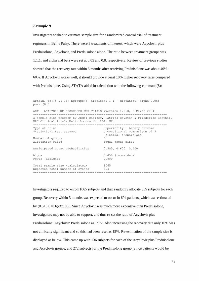
Example 9
Investigators wished to estimate sample size for a randomized control trial of treatment
regimens in Bell’s Palsy. There were 3 treatments of interest, which were Acyclovir plus
Prednisolone, Acyclovir, and Prednisolone alone. The ratio between treatment groups was
1:1:1, and alpha and beta were set at 0.05 and 0.8, respectively. Review of previous studies
showed that the recovery rate within 3 months after receiving Prednisolone was about 40%-
60%. If Acyclovir works well, it should provide at least 10% higher recovery rates compared
with Prednisolone. Using STATA aided in calculation with the following command(8):
artbin, pr(.5 .6 .6) ngroups(3) aratios(1 1 1 ) distant(0) alpha(0.05)
power(0.8)
ART - ANALYSIS OF RESOURCES FOR TRIALS (version 1.0.0, 3 March 2004)
--------------------------------------------------------------------------
A sample size program by Abdel Babiker, Patrick Royston & Friederike Barthel,
MRC Clinical Trials Unit, London NW1 2DA, UK.
--------------------------------------------------------------------------
Type of trial Superiority - binary outcome
Statistical test assumed Unconditional comparison of 3
binomial proportions
Number of groups 3
Allocation ratio Equal group sizes
Anticipated event probabilities 0.500, 0.600, 0.600
Alpha 0.050 (two-sided)
Power (designed) 0.800
Total sample size (calculated) 1065
Expected total number of events 604
--------------------------------------------------------------------------
Investigators required to enroll 1065 subjects and then randomly allocate 355 subjects for each
group. Recovery within 3 months was expected to occur in 604 patients, which was estimated
by (0.5+0.6+0.6)/3x1065. Since Acyclovir was much more expensive than Prednisolone,
investigators may not be able to support, and thus re-set the ratio of Acyclovir plus
Prednisolone: Acyclovir: Prednisolone as 1:1:2. Also increasing the recovery rate only 10% was
not clinically significant and so this had been reset as 15%. Re-estimation of the sample size is
displayed as below. This came up with 136 subjects for each of the Acyclovir plus Prednisolone
and Acyclovir groups, and 272 subjects for the Prednisolone group. Since patients would be
35
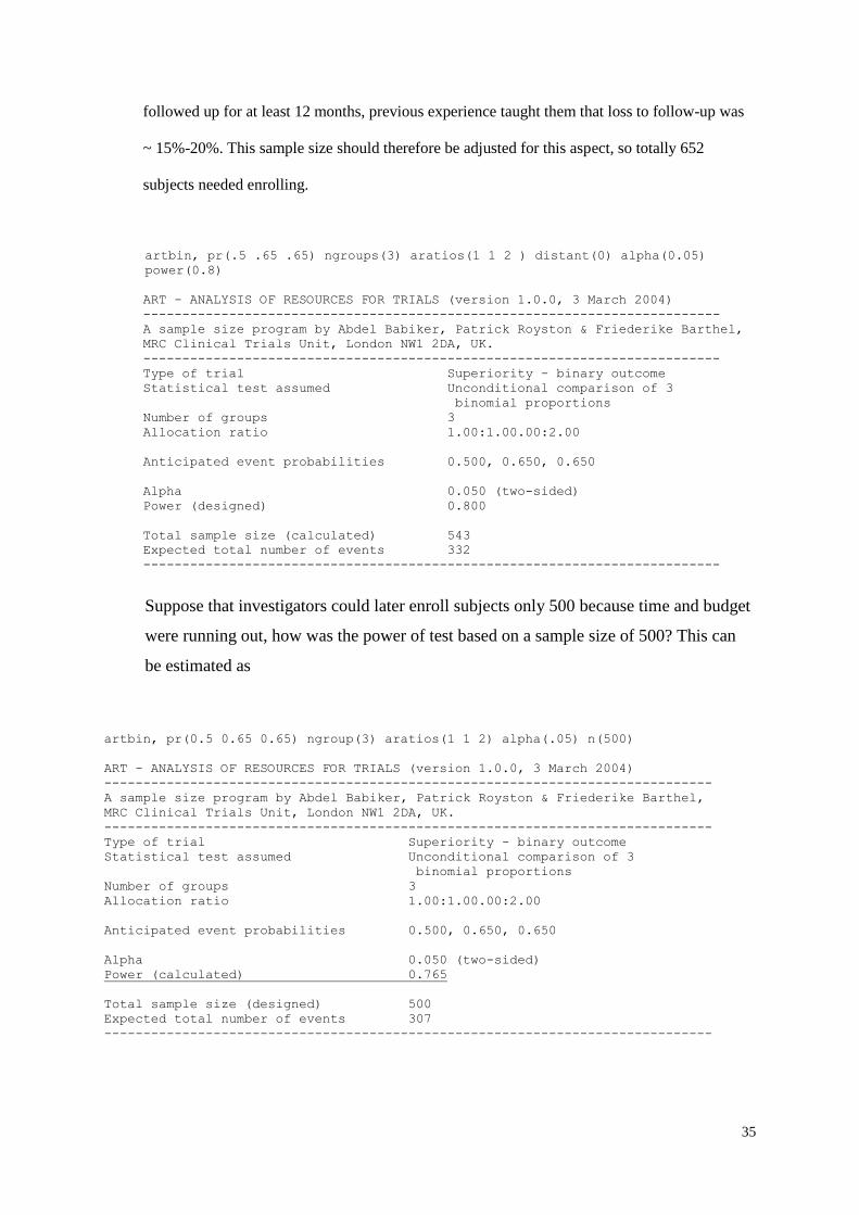
followed up for at least 12 months, previous experience taught them that loss to follow-up was
~ 15%-20%. This sample size should therefore be adjusted for this aspect, so totally 652
subjects needed enrolling.
artbin, pr(.5 .65 .65) ngroups(3) aratios(1 1 2 ) distant(0) alpha(0.05)
power(0.8)
ART - ANALYSIS OF RESOURCES FOR TRIALS (version 1.0.0, 3 March 2004)
--------------------------------------------------------------------------
A sample size program by Abdel Babiker, Patrick Royston & Friederike Barthel,
MRC Clinical Trials Unit, London NW1 2DA, UK.
--------------------------------------------------------------------------
Type of trial Superiority - binary outcome
Statistical test assumed Unconditional comparison of 3
binomial proportions
Number of groups 3
Allocation ratio 1.00:1.00.00:2.00
Anticipated event probabilities 0.500, 0.650, 0.650
Alpha 0.050 (two-sided)
Power (designed) 0.800
Total sample size (calculated) 543
Expected total number of events 332
--------------------------------------------------------------------------
Suppose that investigators could later enroll subjects only 500 because time and budget
were running out, how was the power of test based on a sample size of 500? This can
be estimated as
artbin, pr(0.5 0.65 0.65) ngroup(3) aratios(1 1 2) alpha(.05) n(500)
ART - ANALYSIS OF RESOURCES FOR TRIALS (version 1.0.0, 3 March 2004)
------------------------------------------------------------------------------
A sample size program by Abdel Babiker, Patrick Royston & Friederike Barthel,
MRC Clinical Trials Unit, London NW1 2DA, UK.
------------------------------------------------------------------------------
Type of trial Superiority - binary outcome
Statistical test assumed Unconditional comparison of 3
binomial proportions
Number of groups 3
Allocation ratio 1.00:1.00.00:2.00
Anticipated event probabilities 0.500, 0.650, 0.650
Alpha 0.050 (two-sided)
Power (calculated) 0.765
Total sample size (designed) 500
Expected total number of events 307
------------------------------------------------------------------------------
36
Two independent means
The outcome of interest can be continuous data, such as
- Bone mineral density between calcium supplement versus placebo
- Estimated GFR (or serum creatinine) between controlled and un-controlled
blood sugar groups in diabetic patients
- Systolic/diastolic blood pressure between angiotensin-receptor blocker (ARB) and
ACEI in diabetic patients
- Level of HbA1C between patients who received Rosiglitazone versus other
glycemic drugs
- Pain scores of arthritis patients who receive Celecoxib and Ibuprofen
These outcomes are mostly intermediate or surrogate of the final outcomes. The drawback of
these can be studied more in the RCT course, but the benefit is that it is usually needs a smaller
sample size than comparison of dichotomous (proportion) or time to event outcomes. In case
that the investigators do not have much time to follow up, the interested clinical endpoint also
takes long time to occur, and/or investigators do not have enough budget to run a longer-period
project, they usually come up with comparison of continuous outcomes. The concept of sample
size estimation is the same as for proportions. That is the false positive and false negative are
needed to assign before conducting the study. Information we need to gather from previous
studies are the mean and standard deviation of interested values in the control or standard
treatment group. Finally, the size of difference to be able to detect needs calibrating or
justifying considering clinical significance and feasibility for conducting the study. The null
hypothesis and equation used for sample size calculation are as follows:
Ho: 1 -2= 0
Ha: 1-2 0 2
21
βα/2
μμr
σZZrn
)(
)1)x((
37
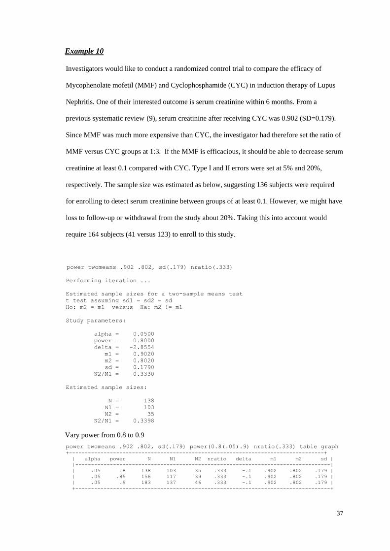
Example 10
Investigators would like to conduct a randomized control trial to compare the efficacy of
Mycophenolate mofetil (MMF) and Cyclophosphamide (CYC) in induction therapy of Lupus
Nephritis. One of their interested outcome is serum creatinine within 6 months. From a
previous systematic review (9), serum creatinine after receiving CYC was 0.902 (SD=0.179).
Since MMF was much more expensive than CYC, the investigator had therefore set the ratio of
MMF versus CYC groups at 1:3. If the MMF is efficacious, it should be able to decrease serum
creatinine at least 0.1 compared with CYC. Type I and II errors were set at 5% and 20%,
respectively. The sample size was estimated as below, suggesting 136 subjects were required
for enrolling to detect serum creatinine between groups of at least 0.1. However, we might have
loss to follow-up or withdrawal from the study about 20%. Taking this into account would
require 164 subjects (41 versus 123) to enroll to this study.
power twomeans .902 .802, sd(.179) nratio(.333)
Performing iteration ...
Estimated sample sizes for a two-sample means test
t test assuming sd1 = sd2 = sd
Ho: m2 = m1 versus Ha: m2 != m1
Study parameters:
alpha = 0.0500
power = 0.8000
delta = -2.8554
m1 = 0.9020
m2 = 0.8020
sd = 0.1790
N2/N1 = 0.3330
Estimated sample sizes:
N = 138
N1 = 103
N2 = 35
N2/N1 = 0.3398
Vary power from 0.8 to 0.9
power twomeans .902 .802, sd(.179) power(0.8(.05).9) nratio(.333) table graph
+---------------------------------------------------------------------------------+
| alpha power N N1 N2 nratio delta m1 m2 sd |
|---------------------------------------------------------------------------------|
| .05 .8 138 103 35 .333 -.1 .902 .802 .179 |
| .05 .85 156 117 39 .333 -.1 .902 .802 .179 |
| .05 .9 183 137 46 .333 -.1 .902 .802 .179 |
+---------------------------------------------------------------------------------+
38
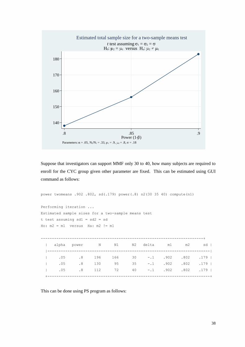
Suppose that investigators can support MMF only 30 to 40, how many subjects are required to
enroll for the CYC group given other parameter are fixed. This can be estimated using GUI
command as follows:
power twomeans .902 .802, sd(.179) power(.8) n2(30 35 40) compute(n1)
Performing iteration ...
Estimated sample sizes for a two-sample means test
t test assuming sd1 = sd2 = sd
Ho: m2 = m1 versus Ha: m2 != m1
-------------------------------------------------------------------------+
| alpha power N N1 N2 delta m1 m2 sd |
|-------------------------------------------------------------------------|
| .05 .8 196 166 30 -.1 .902 .802 .179 |
| .05 .8 130 95 35 -.1 .902 .802 .179 |
| .05 .8 112 72 40 -.1 .902 .802 .179 |
+-------------------------------------------------------------------------+
This can be done using PS program as follows:
140
150
160
170
180
To
tal
sam
ple
siz
e (N
)
.8 .85 .9Power (1- )
Parameters: = .05, N2/N1 = .33, 1 = .9, 2 = .8, = .18
t test assuming 1 = 2 = H0: 2 = 1 versus Ha: 2 1
Estimated total sample size for a two-sample means test
39
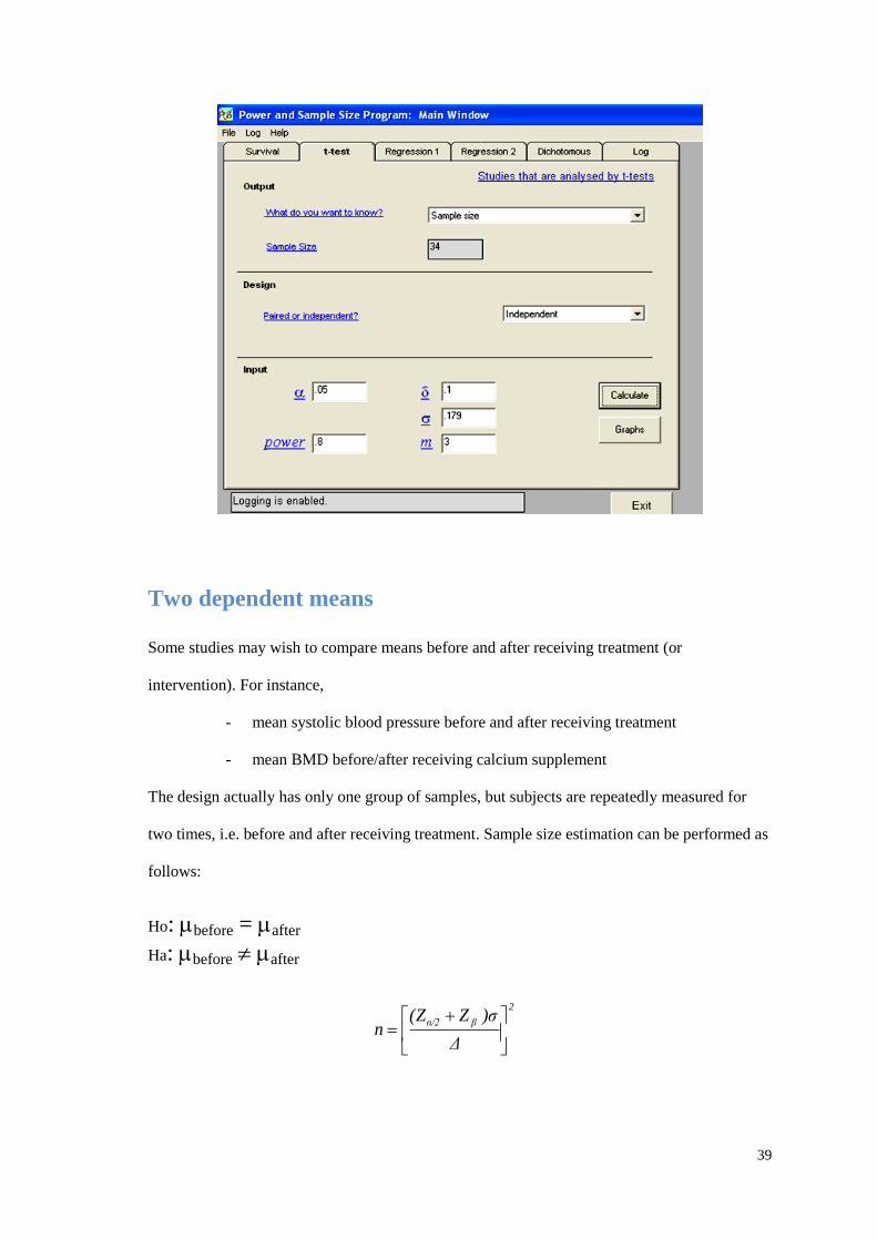
Two dependent means
Some studies may wish to compare means before and after receiving treatment (or
intervention). For instance,
- mean systolic blood pressure before and after receiving treatment
- mean BMD before/after receiving calcium supplement
The design actually has only one group of samples, but subjects are repeatedly measured for
two times, i.e. before and after receiving treatment. Sample size estimation can be performed as
follows:
Ho: before = after
Ha: before after
2
βα/2
Δ
)σZ(Zn
40
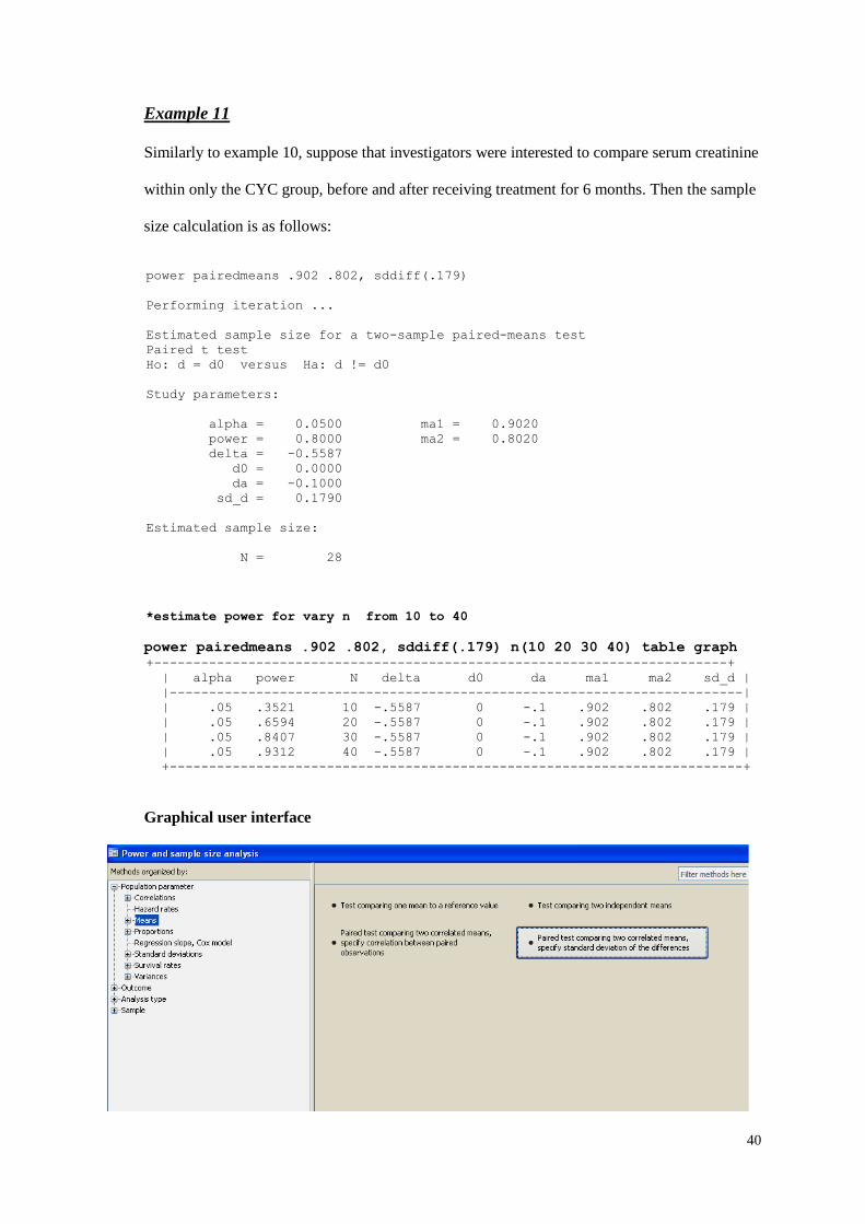
Example 11
Similarly to example 10, suppose that investigators were interested to compare serum creatinine
within only the CYC group, before and after receiving treatment for 6 months. Then the sample
size calculation is as follows:
power pairedmeans .902 .802, sddiff(.179)
Performing iteration ...
Estimated sample size for a two-sample paired-means test
Paired t test
Ho: d = d0 versus Ha: d != d0
Study parameters:
alpha = 0.0500 ma1 = 0.9020
power = 0.8000 ma2 = 0.8020
delta = -0.5587
d0 = 0.0000
da = -0.1000
sd_d = 0.1790
Estimated sample size:
N = 28
*estimate power for vary n from 10 to 40
power pairedmeans .902 .802, sddiff(.179) n(10 20 30 40) table graph +-------------------------------------------------------------------------+
| alpha power N delta d0 da ma1 ma2 sd_d |
|-------------------------------------------------------------------------|
| .05 .3521 10 -.5587 0 -.1 .902 .802 .179 |
| .05 .6594 20 -.5587 0 -.1 .902 .802 .179 |
| .05 .8407 30 -.5587 0 -.1 .902 .802 .179 |
| .05 .9312 40 -.5587 0 -.1 .902 .802 .179 |
+-------------------------------------------------------------------------+
Graphical user interface
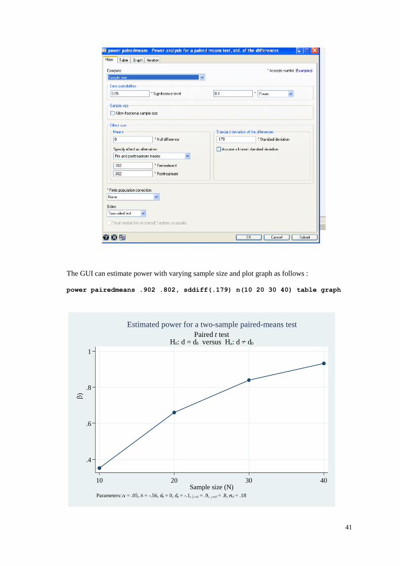
41
The GUI can estimate power with varying sample size and plot graph as follows :
power pairedmeans .902 .802, sddiff(.179) n(10 20 30 40) table graph
.4
.6
.8
1
Po
wer
(1
-
)
10 20 30 40Sample size (N)
Parameters: = .05, = -.56, d0 = 0, da = -.1, a1 = .9, a2 = .8, d = .18
Paired t testH0: d = d0 versus Ha: d d0
Estimated power for a two-sample paired-means test
42
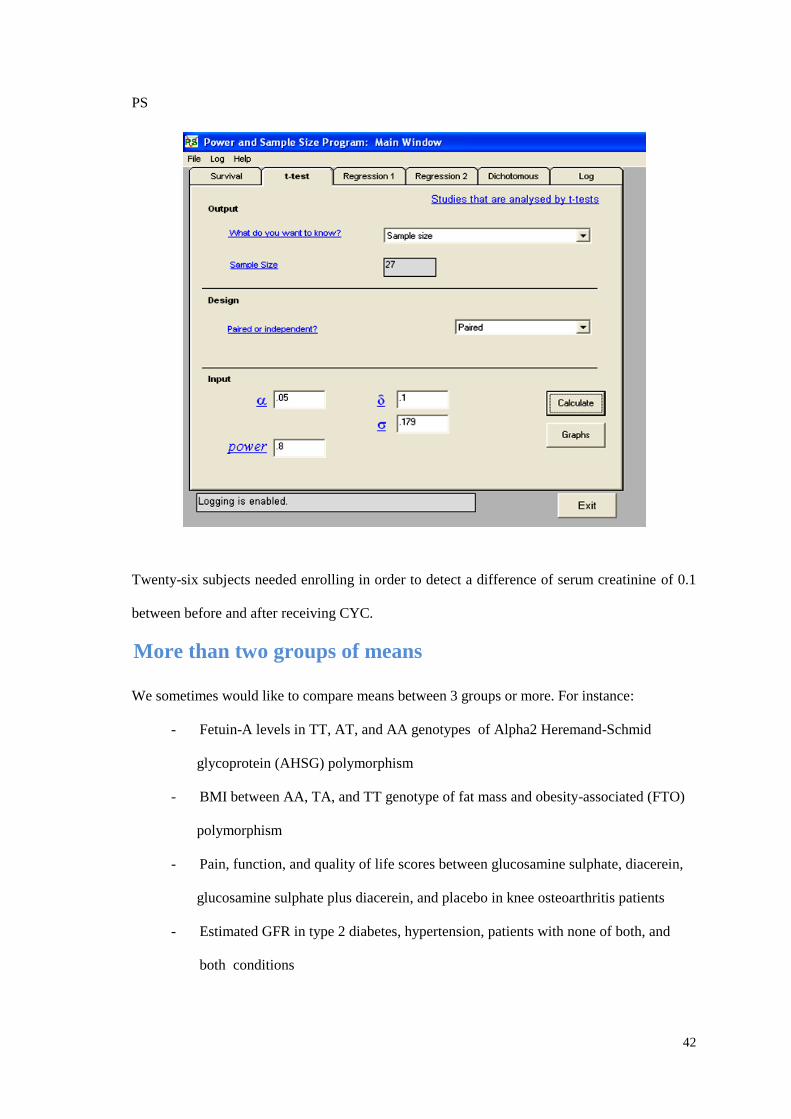
PS
Twenty-six subjects needed enrolling in order to detect a difference of serum creatinine of 0.1
between before and after receiving CYC.
More than two groups of means
We sometimes would like to compare means between 3 groups or more. For instance:
- Fetuin-A levels in TT, AT, and AA genotypes of Alpha2 Heremand-Schmid
glycoprotein (AHSG) polymorphism
- BMI between AA, TA, and TT genotype of fat mass and obesity-associated (FTO)
polymorphism
- Pain, function, and quality of life scores between glucosamine sulphate, diacerein,
glucosamine sulphate plus diacerein, and placebo in knee osteoarthritis patients
- Estimated GFR in type 2 diabetes, hypertension, patients with none of both, and
both conditions
43
There are STATA user-written commands by the UCLA group (10) (i.e., fpower and simpower)
that can estimate a sample size for this purpose. This is demonstrated as shown in the example
below:
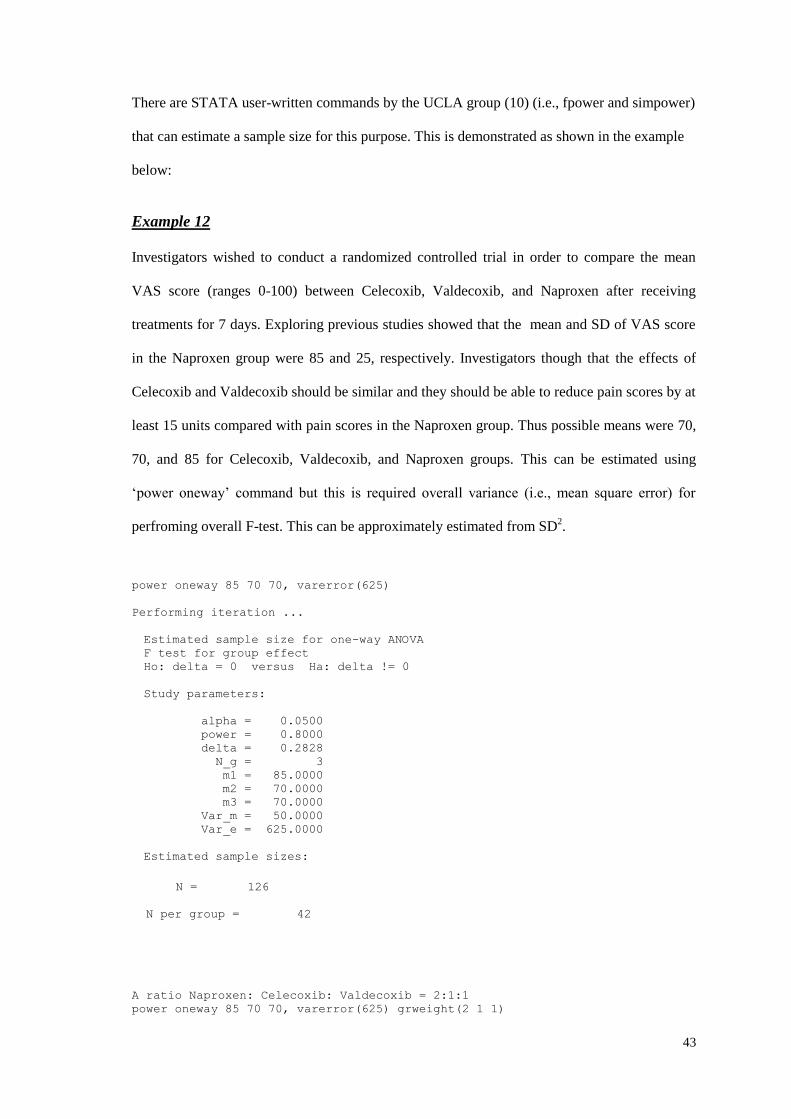
Example 12
Investigators wished to conduct a randomized controlled trial in order to compare the mean
VAS score (ranges 0-100) between Celecoxib, Valdecoxib, and Naproxen after receiving
treatments for 7 days. Exploring previous studies showed that the mean and SD of VAS score
in the Naproxen group were 85 and 25, respectively. Investigators though that the effects of
Celecoxib and Valdecoxib should be similar and they should be able to reduce pain scores by at
least 15 units compared with pain scores in the Naproxen group. Thus possible means were 70,
70, and 85 for Celecoxib, Valdecoxib, and Naproxen groups. This can be estimated using
‘power oneway’ command but this is required overall variance (i.e., mean square error) for
perfroming overall F-test. This can be approximately estimated from SD2.
power oneway 85 70 70, varerror(625)
Performing iteration ...
Estimated sample size for one-way ANOVA
F test for group effect
Ho: delta = 0 versus Ha: delta != 0
Study parameters:
alpha = 0.0500
power = 0.8000
delta = 0.2828
N_g = 3
m1 = 85.0000
m2 = 70.0000
m3 = 70.0000
Var_m = 50.0000
Var_e = 625.0000
Estimated sample sizes:
N = 126
N per group = 42
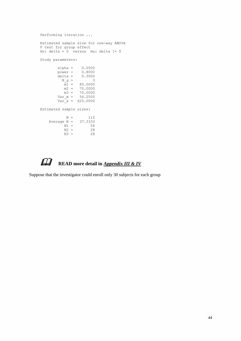
A ratio Naproxen: Celecoxib: Valdecoxib = 2:1:1
power oneway 85 70 70, varerror(625) grweight(2 1 1)
44
Performing iteration ...
Estimated sample size for one-way ANOVA
F test for group effect
Ho: delta = 0 versus Ha: delta != 0
Study parameters:
alpha = 0.0500
power = 0.8000
delta = 0.3000
N_g = 3
m1 = 85.0000
m2 = 70.0000
m3 = 70.0000
Var_m = 56.2500
Var_e = 625.0000
Estimated sample sizes:
N = 112
Average N = 37.3333
N1 = 56
N2 = 28
N3 = 28
READ more detail in Appendix III & IV Suppose that the investigator could enroll only 30 subjects for each group
45
TEST FOR EQUIVALENCE
Continuous data
READ Appendix III (Statist Med 2004; 23: 1921)
Some clinical researchers aim to determine whether a new treatment has the same clinical
effect as the standard treatment one. In this case, the concepts of hypothesis testing, type I and
II errors, and sample size estimation are different compared to those studies which aim to test
for difference or superiority. The null and alternative hypotheses for equivalent studies are
opposite to difference/superiority studies. For instance,
Ho: Mean values are different between groups (Ho: µA≠µB)
Ha: Mean values are not different between groups (Ha: µA = µ)
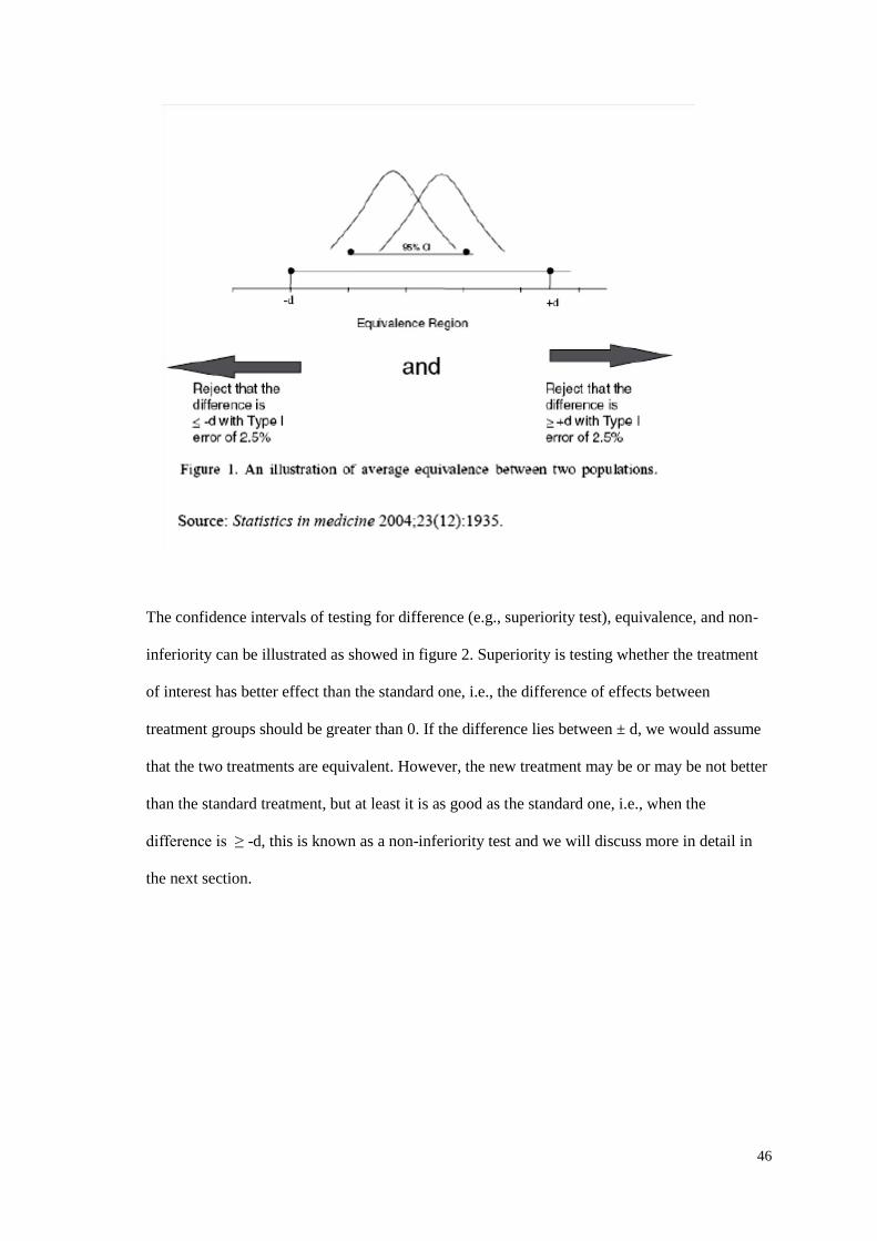
However, when we said the two treatments are equivalent they are actually not exactly
equivalent, which leads us to define a region or margin of equivalence (11). For instance, the
two treatments are claimed to be similarly effective if the difference (µA - µB) falls between -d
and +d and they are different if (µA - µB) is ≤ -d or (µA - µB) ≥ +d, as described in the figure
below. Thus, the null and alternative hypotheses are:
Ho: µA - µB ≤ -d or µA - µB ≥ +d
Ha: -d < µA - µB < +d
The null hypothesis consists of a pair of one-sided tests, i.e., treatment A is superior (µA - µB ≥
+d ), and treatment A is inferior to the treatment B (µA - µB ≤ -d). The alternative hypothesis
states that treatment A is equivalent to treatment B if the difference falls within the margins. In
order to accept that the two treatment effects are equivalent, we need to reject both of the one-
sided tests in the null hypothesis. Once the null hypothesis is rejected, there are an errors, i.e.,
type I and II errors.
46
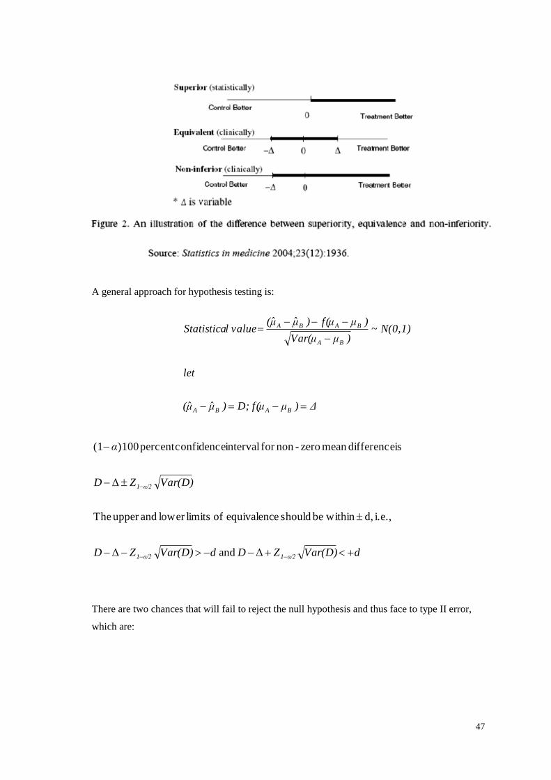
The confidence intervals of testing for difference (e.g., superiority test), equivalence, and non-
inferiority can be illustrated as showed in figure 2. Superiority is testing whether the treatment
of interest has better effect than the standard one, i.e., the difference of effects between
treatment groups should be greater than 0. If the difference lies between ± d, we would assume
that the two treatments are equivalent. However, the new treatment may be or may be not better
than the standard treatment, but at least it is as good as the standard one, i.e., when the
difference is ≥ -d, this is known as a non-inferiority test and we will discuss more in detail in
the next section.
47
A general approach for hypothesis testing is:
dVar(D)ZDdVar(D)ZD
Var(D)ZD
α
α/21α/21
α/21
Δ and Δ
i.e., d, within be should eequivalenc of limitslower andupper The
Δ
is differencemean zero-nonfor interval confidencepercent )100(1
There are two chances that will fail to reject the null hypothesis and thus face to type II error,
which are:
Δ)μf (μD;)μμ(
let
N(0,1)~)μVar(μ
)μf (μ)μμ(value lStatistica
BABA
BA
BABA
ˆˆ
ˆˆ
48
)Z(Z
dVar(D)
ZVar(D)
dZ
ZVar(D)
dZ
β/2ββ ,βββ
ZVar(D)
dZ
ZVar(D)
dZ
Var(D)ZVar(D)Zd
Var(D)ZVar(D)Zd
2
α1β/21
2
α/21β/21
α/21β/21
2121
α/21β1
α/11β1
α/21β1
α/21β1
2
1
2
1
0Δ If
Δ
where
Δ
andΔ
Thus
Δ
andΔ
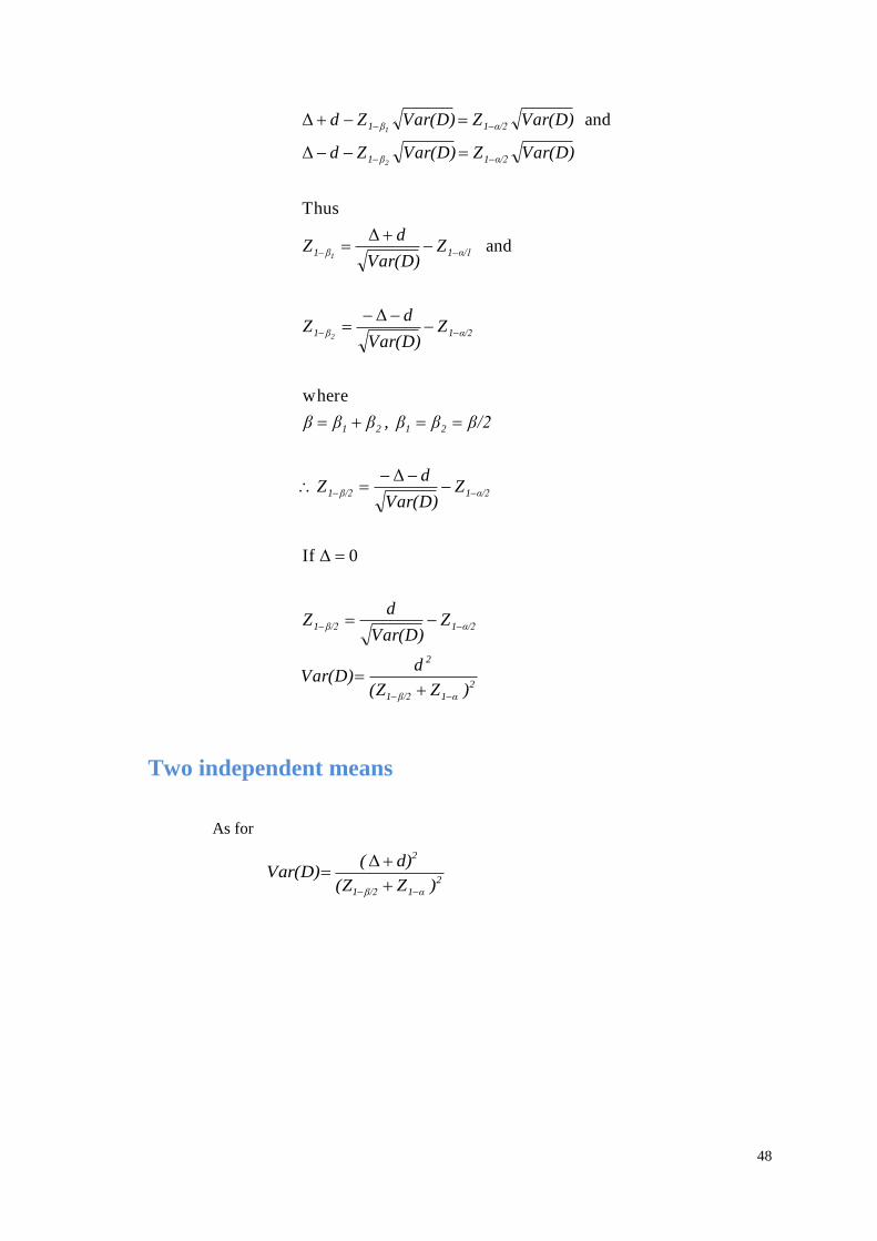
Two independent means
As for
2
α1β/21
2
)Z(Z
d)(Var(D)
Δ
49
α11
2
22
α/21β/21
1
2
α/21β1
2
1
2
1
2
12
1
2
2
2
1
2
Zσ
d)(Δ
1)(r
rnΦ12xβ1
d)(Δ
σ)Z(Z
r
1rn
)Z(Z
d)(Δ
n
σ
r
1r
n
σ
r
1rVar(D)
rnn
rn
n
let
n
σ
n
σVar(D)
istest ofPower
Special case is if ∆ = 0
2
22
α/21β/21
1d
σ)Z(Z
r
1rn
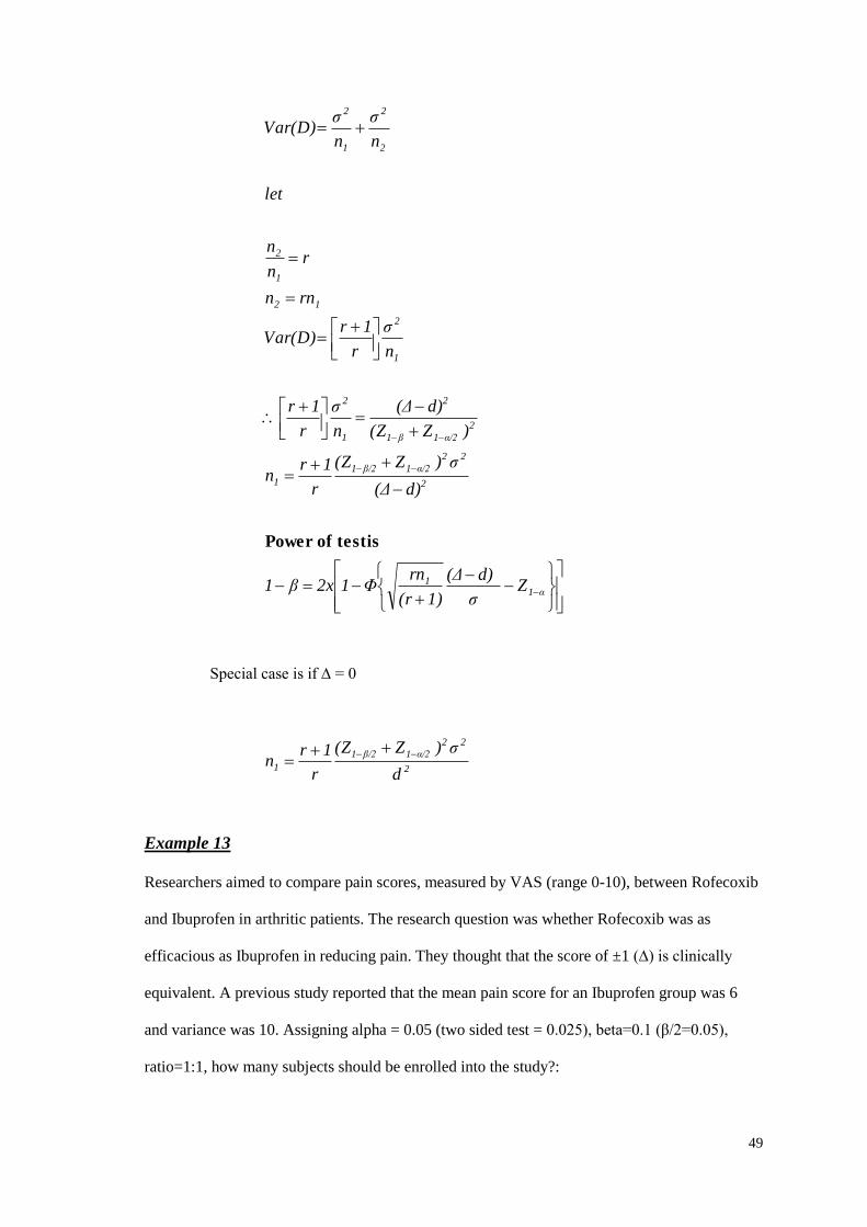
Example 13
Researchers aimed to compare pain scores, measured by VAS (range 0-10), between Rofecoxib
and Ibuprofen in arthritic patients. The research question was whether Rofecoxib was as
efficacious as Ibuprofen in reducing pain. They thought that the score of ±1 (∆) is clinically
equivalent. A previous study reported that the mean pain score for an Ibuprofen group was 6
and variance was 10. Assigning alpha = 0.05 (two sided test = 0.025), beta=0.1 (β/2=0.05),
ratio=1:1, how many subjects should be enrolled into the study?:
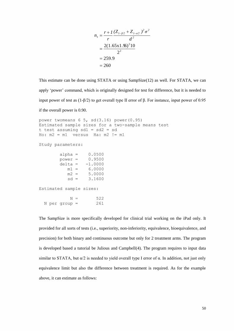
50
602
259.9
2
106)2(1.65x1.92
2
2
22
α/21β/21
1d
σ)Z(Z
r
1rn
This estimate can be done using STATA or using SampSize(12) as well. For STATA, we can
apply ‘power’ command, which is originally designed for test for difference, but it is needed to
input power of test as (1-β/2) to get overall type II error of β. For instance, input power of 0.95
if the overall power is 0.90.
power twomeans 6 5, sd(3.16) power(0.95)
Estimated sample sizes for a two-sample means test
t test assuming sd1 = sd2 = sd
Ho: m2 = m1 versus Ha: m2 != m1
Study parameters:
alpha = 0.0500
power = 0.9500
delta = -1.0000
m1 = 6.0000
m2 = 5.0000
sd = 3.1600
Estimated sample sizes:
N = 522
N per group = 261
The SampSize is more specifically developed for clinical trial working on the iPad only. It
provided for all sorts of tests (i.e., superiority, non-inferiority, equivalence, bioequivalence, and
precision) for both binary and continuous outcome but only for 2 treatment arms. The program
is developed based a tutorial be Julious and Campbell(4). The program requires to input data
similar to STATA, but α/2 is needed to yield overall type I error of α. In addition, not just only
equivalence limit but also the difference between treatment is required. As for the example
above, it can estimate as follows:
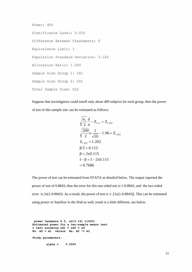
51
Power: 90%
Significance Level: 0.025
Difference Between Treatments: 0
Equivalence Limit: 1
Population Standard Deviation: 3.162
Allocation Ratio: 1.000
Sample Size Group 1: 261
Sample Size Group 2: 261
Total Sample Size: 522
Suppose that investigators could enroll only about 400 subjects for each group, then the power
of test of this sample size can be estimated as follows:
.76860
2x0.1151β1
2x0.115β
.1150β/2
1.202Z
Z1.9610
1x
2
200
ZZσ
d
2
n
β/21
β/21
β/21α11
The power of test can be estimated from STATA as detailed below. The output reported the
power of test of 0.8843, thus the error for this one-sided test is 1-0.8843, and the two-sided
error is 2x(1-0.8843). As a result, the power of test is 1- [2x(1-0.8843)]. This can be estimated
using power or SamSize in the iPad as well, result is a little different, see below.
power twomeans 6 5, sd(3.16) n(400)
Estimated power for a two-sample means test
t test assuming sd1 = sd2 = sd
Ho: m2 = m1 versus Ha: m2 != m1
Study parameters:
alpha = 0.0500
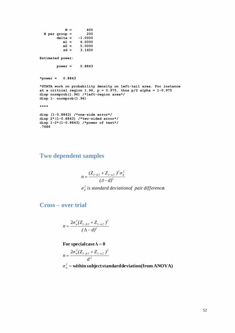
52
N = 400
N per group = 200
delta = -1.0000
m1 = 6.0000
m2 = 5.0000
sd = 3.1600
Estimated power:
power = 0.8843
*power = 0.8843
*STATA work on probability density on left-tail area. For instance
at a critical region 1.96, p = 0.975, thus p/2 alpha = 1-0.975
disp normprob(1.96) /*left-region area*/
disp 1- normprob(1.96)
****
disp (1-0.8843) /*one-side error*/
disp 2*(1-0.8843) /*two-sided error*/
disp 1-2*(1-0.8843) /*power of test*/
.7686
Two dependent samples
sdif ference pair of deviation standardis σ
d)(Δ
σ)Z(Zn
2
d
2
2
d
2
α/21β/21
Cross – over trial
ANOVA)(from deviation standardsubject within
0Δ case specialFor
2
w
2
2
α/21β/21
2
w
2
2
α/21β/21
2
w
σ
d
)Z(Zσn
d)(
)Z(Zσn
2
Δ
2
53
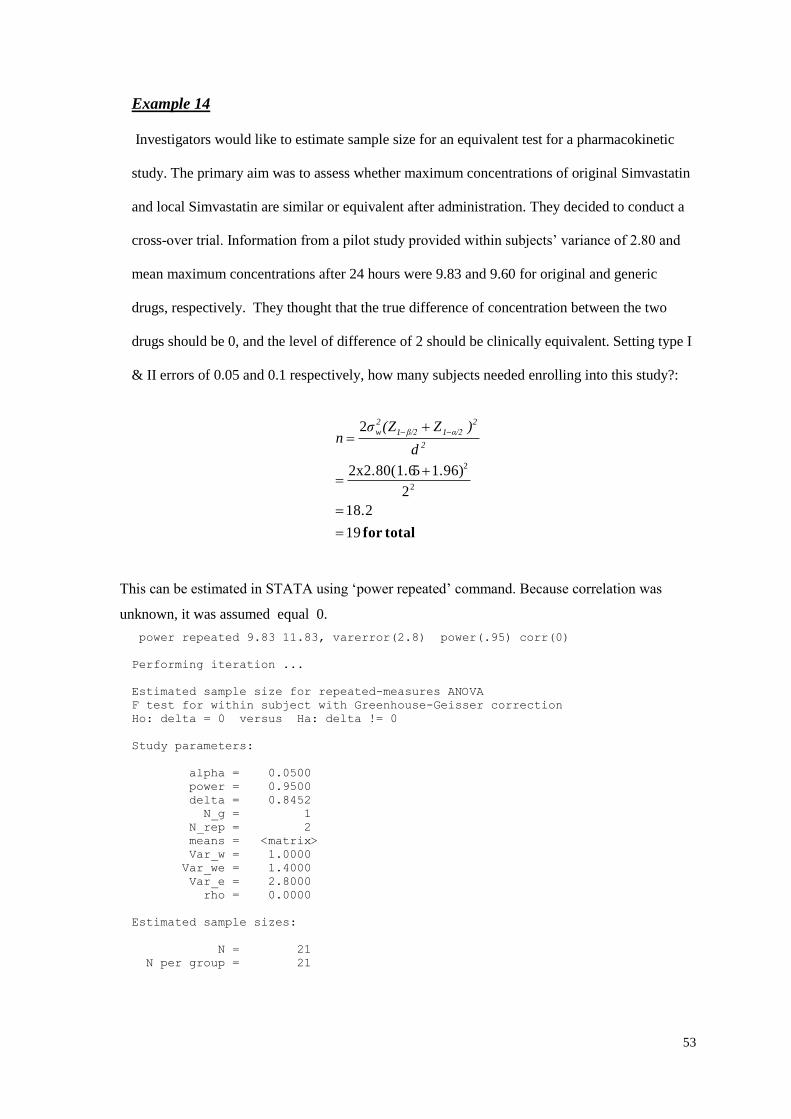
Example 14
Investigators would like to estimate sample size for an equivalent test for a pharmacokinetic
study. The primary aim was to assess whether maximum concentrations of original Simvastatin
and local Simvastatin are similar or equivalent after administration. They decided to conduct a
cross-over trial. Information from a pilot study provided within subjects’ variance of 2.80 and
mean maximum concentrations after 24 hours were 9.83 and 9.60 for original and generic
drugs, respectively. They thought that the true difference of concentration between the two
drugs should be 0, and the level of difference of 2 should be clinically equivalent. Setting type I
& II errors of 0.05 and 0.1 respectively, how many subjects needed enrolling into this study?:
totalfor 19
18.2
2
1.96)52x2.80(1.6
2
2
2
2
2
α/21β/21
2
w
d
)Z(Zσn
This can be estimated in STATA using ‘power repeated’ command. Because correlation was
unknown, it was assumed equal 0.
power repeated 9.83 11.83, varerror(2.8) power(.95) corr(0)
Performing iteration ...
Estimated sample size for repeated-measures ANOVA
F test for within subject with Greenhouse-Geisser correction
Ho: delta = 0 versus Ha: delta != 0
Study parameters:
alpha = 0.0500
power = 0.9500
delta = 0.8452
N_g = 1
N_rep = 2
means = <matrix>
Var_w = 1.0000
Var_we = 1.4000
Var_e = 2.8000
rho = 0.0000
Estimated sample sizes:
N = 21
N per group = 21
54
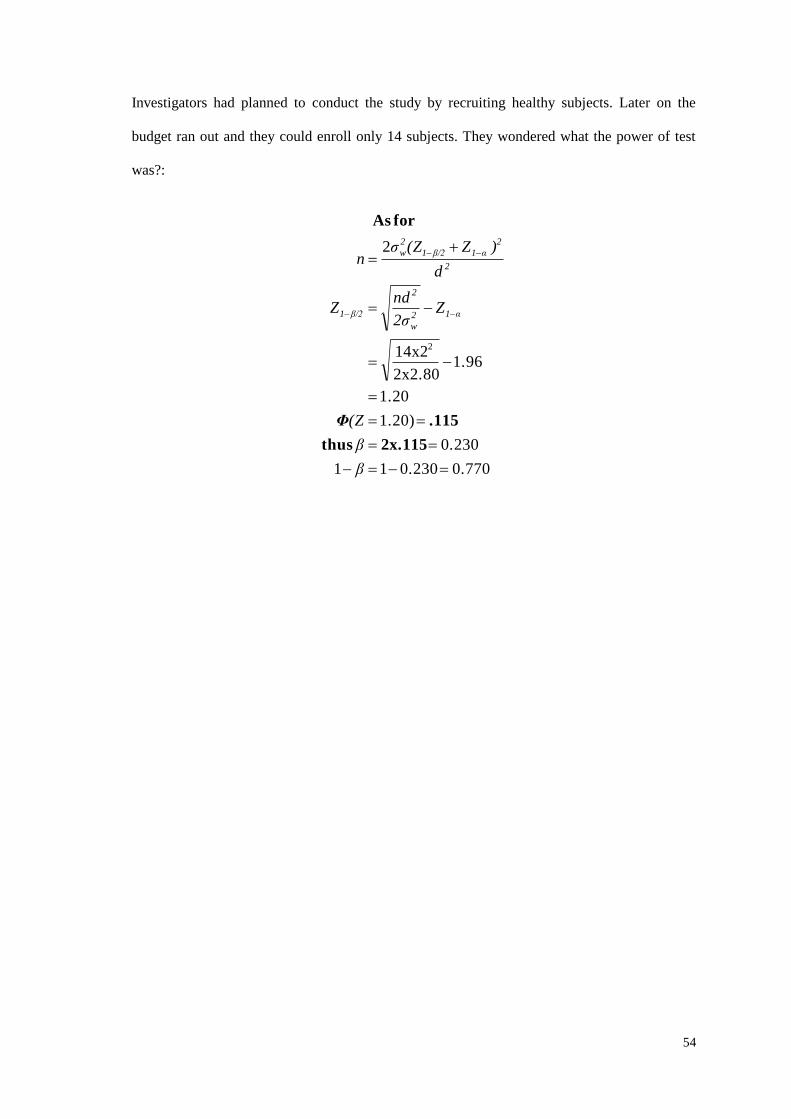
Investigators had planned to conduct the study by recruiting healthy subjects. Later on the
budget ran out and they could enroll only 14 subjects. They wondered what the power of test
was?:
0.7700.23011
0.230
1.20)
1.20
1.962x2.80
14x2
2
2
β
β
(Z
Z2σ
ndZ
d
)Z(Zσn
α12
w
2
β/21
2
2
α1β/21
2
w
2x.115thus
.115
for As
Φ
55
NON – INFERIORITY
Continuous data
The new treatment A is said to be non-inferior to treatment B if its effect is clinically similar, or
not worse than the treatment B, given that the treatment B is a standard-active control (11, 13).
Suppose that the level of interested outcome is continuous and higher value is better treatment
effect.
This null hypothesis and alternative hypothesis are:
H0: An interested treatment is inferior to the standard treatment
dμμ:H BA0
Ha: An interested treatment is as good as or better (non-inferior) to the standard treatment
dμμ:H BAa
Here, -d is a non-inferior margin which indicates how much the treatment A can be inferior to
B, but it is still considered non-inferior. The most difficult for non-inferior design is to set how
close the effect of treatment A should be to treatment B to claim that treatment A is not inferior
to treatment B. The margin d should be set based on statistical and clinical judgments, given
that it should be greater than the effect size of active control B versus placebo. For instance, if
the effect size for B vs placebo is 1, the d margin can be any value between 0-1 (usually 10-
20%), but should not exceed 1. The best way to get information for the effect size of B vs
placebo is to perform a systematic review and apply a meta-analysis to pool effect size across
studies. The range estimate of pooled effect size (i.e., 95% confidence interval) will help
investigators to justify the margin d properly, usually the lower limit is used (13).
56
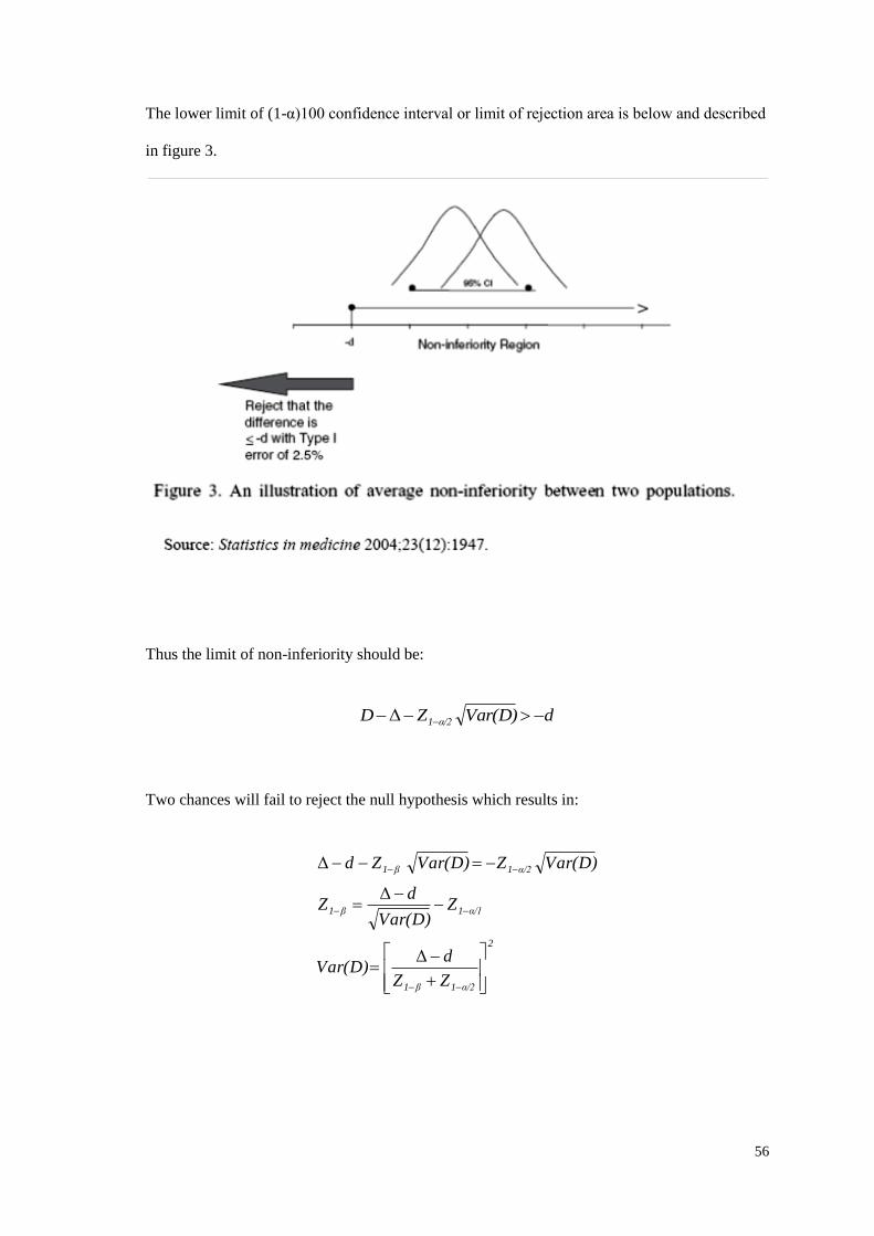
The lower limit of (1-α)100 confidence interval or limit of rejection area is below and described
in figure 3.
Thus the limit of non-inferiority should be:
dVar(D)ZD α/21 Δ
Two chances will fail to reject the null hypothesis which results in:
2
α/21β1
α/11β1
α/21β1
ZZ
dVar(D)
ZVar(D)
dZ
Var(D)ZVar(D)Zd
Δ
Δ
Δ
57
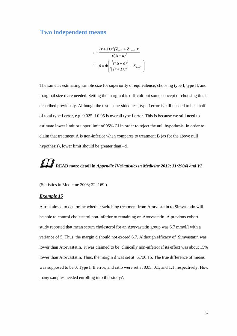
Two independent means
α/212
2
2
2
α/21β1
2
Z1)σ(r
d)r(β
d)r(
)Z(Z)σ(rn
ΔΦ1
Δ
1
The same as estimating sample size for superiority or equivalence, choosing type I, type II, and
marginal size d are needed. Setting the margin d is difficult but some concept of choosing this is
described previously. Although the test is one-sided test, type I error is still needed to be a half
of total type I error, e.g. 0.025 if 0.05 is overall type I error. This is because we still need to
estimate lower limit or upper limit of 95% CI in order to reject the null hypothesis. In order to
claim that treatment A is non-inferior when compares to treatment B (as for the above null
hypothesis), lower limit should be greater than –d.
READ more detail in Appendix IV(Statistics in Medicine 2012; 31:2904) and VI
(Statistics in Medicine 2003; 22: 169.)
Example 15
A trial aimed to determine whether switching treatment from Atorvastatin to Simvastatin will
be able to control cholesterol non-inferior to remaining on Atorvastatin. A previous cohort
study reported that mean serum cholesterol for an Atorvastatin group was 6.7 mmol/l with a
variance of 5. Thus, the margin d should not exceed 6.7. Although efficacy of Simvastatin was
lower than Atorvastatin, it was claimed to be clinically non-inferior if its effect was about 15%
lower than Atorvastatin. Thus, the margin d was set at 6.7x0.15. The true difference of means
was supposed to be 0. Type I, II error, and ratio were set at 0.05, 0.1, and 1:1 ,respectively. How
many samples needed enrolling into this study?:
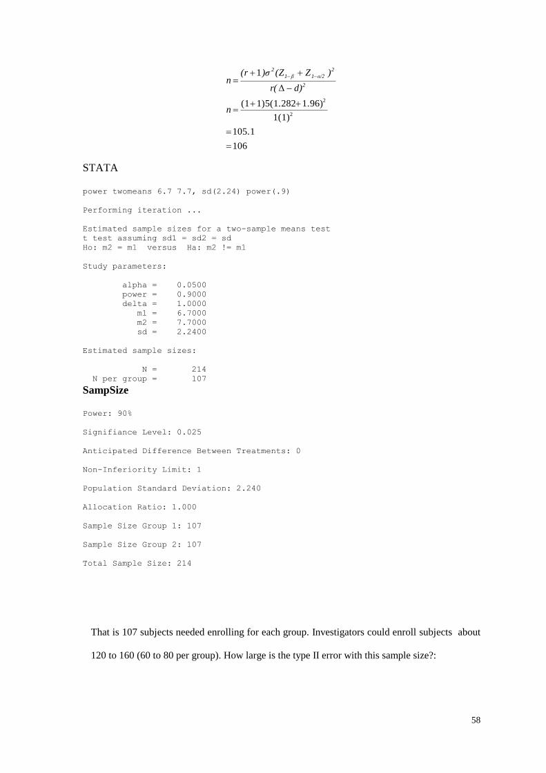
58
106
105.1
1(1)
1.96)1)5(1.282(1
Δ
1
2
2
n
d)r(
)Z(Z)σ(rn
2
2
α/21β1
2
STATA
power twomeans 6.7 7.7, sd(2.24) power(.9)
Performing iteration ...
Estimated sample sizes for a two-sample means test
t test assuming sd1 = sd2 = sd
Ho: m2 = m1 versus Ha: m2 != m1
Study parameters:
alpha = 0.0500
power = 0.9000
delta = 1.0000
m1 = 6.7000
m2 = 7.7000
sd = 2.2400
Estimated sample sizes:
N = 214
N per group = 107
SampSize
Power: 90%
Signifiance Level: 0.025
Anticipated Difference Between Treatments: 0
Non-Inferiority Limit: 1
Population Standard Deviation: 2.240
Allocation Ratio: 1.000
Sample Size Group 1: 107
Sample Size Group 2: 107
Total Sample Size: 214
That is 107 subjects needed enrolling for each group. Investigators could enroll subjects about
120 to 160 (60 to 80 per group). How large is the type II error with this sample size?:
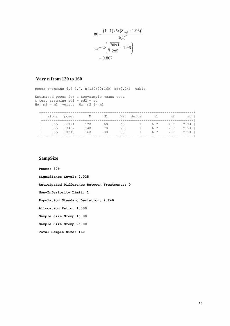
59
0.807
1.962x5
80x1Φ
1(1)
1.96)1)x5x((180
1
2
2
1
β
βZ
Vary n from 120 to 160
power twomeans 6.7 7.7, n(120(20)160) sd(2.24) table
Estimated power for a two-sample means test
t test assuming sd1 = sd2 = sd
Ho: m2 = m1 versus Ha: m2 != m1
+-------------------------------------------------------------------------+
| alpha power N N1 N2 delta m1 m2 sd |
|-------------------------------------------------------------------------|
| .05 .6791 120 60 60 1 6.7 7.7 2.24 |
| .05 .7462 140 70 70 1 6.7 7.7 2.24 |
| .05 .8013 160 80 80 1 6.7 7.7 2.24 |
+-------------------------------------------------------------------------+
SampSize
Power: 80%
Signifiance Level: 0.025
Anticipated Difference Between Treatments: 0
Non-Inferiority Limit: 1
Population Standard Deviation: 2.240
Allocation Ratio: 1.000
Sample Size Group 1: 80
Sample Size Group 2: 80
Total Sample Size: 160
60
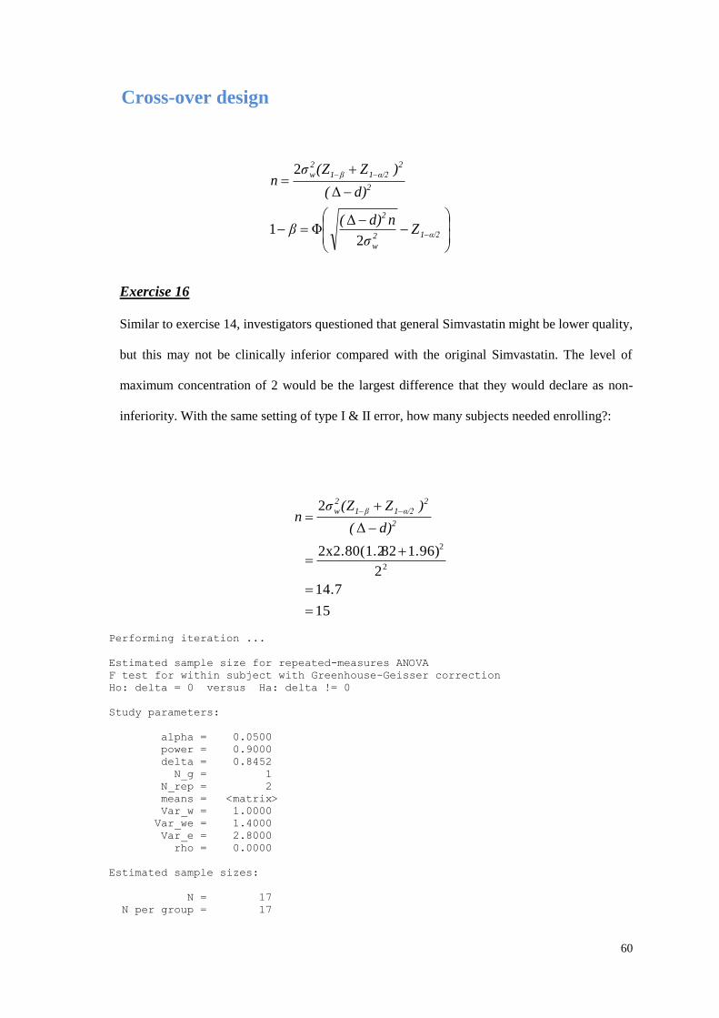
Cross-over design
α/212
w
2
2
2
α/21β1
2
w
Zσ
nd)(β
d)(
)Z(Zσn
2
ΔΦ1
Δ
2
Exercise 16
Similar to exercise 14, investigators questioned that general Simvastatin might be lower quality,
but this may not be clinically inferior compared with the original Simvastatin. The level of
maximum concentration of 2 would be the largest difference that they would declare as non-
inferiority. With the same setting of type I & II error, how many subjects needed enrolling?:
15
14.7
2
1.96)822x2.80(1.2
Δ
2
2
2
2
2
α/21β1
2
w
d)(
)Z(Zσn
Performing iteration ...
Estimated sample size for repeated-measures ANOVA
F test for within subject with Greenhouse-Geisser correction
Ho: delta = 0 versus Ha: delta != 0
Study parameters:
alpha = 0.0500
power = 0.9000
delta = 0.8452
N_g = 1
N_rep = 2
means = <matrix>
Var_w = 1.0000
Var_we = 1.4000
Var_e = 2.8000
rho = 0.0000
Estimated sample sizes:
N = 17
N per group = 17
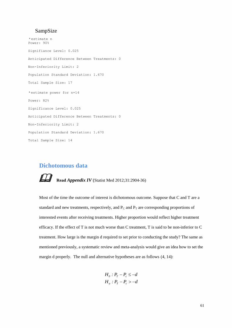
61
SampSize
*estimate n
Power: 90%
Signifiance Level: 0.025
Anticipated Difference Between Treatments: 0
Non-Inferiority Limit: 2
Population Standard Deviation: 1.670
Total Sample Size: 17
*estimate power for n=14
Power: 82%
Significance Level: 0.025
Anticipated Difference Between Treatments: 0
Non-Inferiority Limit: 2
Population Standard Deviation: 1.670
Total Sample Size: 14
Dichotomous data
Read Appendix IV (Statist Med 2012;31:2904-36)
Most of the time the outcome of interest is dichotomous outcome. Suppose that C and T are a
standard and new treatments, respectively, and PC and PT are corresponding proportions of
interested events after receiving treatments. Higher proportion would reflect higher treatment
efficacy. If the effect of T is not much worse than C treatment, T is said to be non-inferior to C
treatment. How large is the margin d required to set prior to conducting the study? The same as
mentioned previously, a systematic review and meta-analysis would give an idea how to set the
margin d properly. The null and alternative hypotheses are as follows (4, 14):
dPP:H
dPP:H
cTa
cT0
62
If the difference between PT and Pc > -d, the null hypothesis is rejected. Type I error for non-
inferior (and also equivalence) study is usually set at a half of type I error for a difference
(superiority) study (4). The reason for the equivalent study is because we need to reject both 2-
sided hypotheses in order to claim that the 2 treatments are equivalent. For a non-inferior
study, although we need to reject only one-sided test, a 95% CI is also needed to estimate.
Regarding the above hypothesis, we need to show that the lower limit (2.5%)–d is exceeded.
The equation used for sample size estimation is as follows (4, 14):
α/21Z)cP(crP)TP(TP
d)cPT(PTnΦβ
α1Z)cP(crP)TP(TP
d)cPT(PTnβ1Z
2d)cPT(P
)cP(crP)TP(TP2)α/21Zβ1(Z
Tn
1111
11
11
Exercise 17
Investigators would like to conduct a non-inferiority RCT in order to compare the incidence of
complete remission between MMF versus Cyclophosphamide. It was claimed that the efficacy
of MMF in reaching disease remission might be little worse than Cyclophosphamide, but
adverse events from use of this drug (e.g., infection, leucopenia, or ovarian failure) occurred
less. The investigators think that if the MMF’s efficacy is not inferior to Cyclophosphamide, it
should be worth prescribing. A previous systematic review and meta-analysis reported that the
incidence of complete remission in Cyclophosphamide was 0.194 (9). If the incidence of
complete remission in MMF is about 20% lower (i.e., 3.88% (d)), this should be clinically non-
inferior. They allowed a true difference equal to 1%, type I & II =0.05 and 0.1 respectively, and
ratio=1:1. How large was the sample size?
63
1011
1010.5049
0388.184.
194.184.1.96.842
2)00(0.194
)00.194()00.184(2)(0
2d)cPT(P
)cP(crP)TP(TP2)α/21Zβ1(Z
Tn
11
11
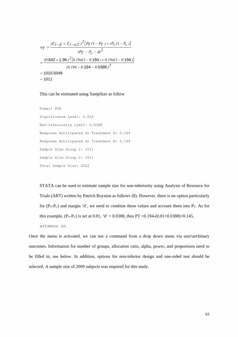
This can be estimated using SampSize as follow
Power: 80%
Significance Level: 0.025
Non-Inferiority Limit: 0.0388
Response Anticipated On Treatment A: 0.184
Response Anticipated On Treatment B: 0.194
Sample Size Group 1: 1011
Sample Size Group 2: 1011
Total Sample Size: 2022
STATA can be used to estimate sample size for non-inferiority using Analysis of Resource for
Trials (ART) written by Patrick Royston as follows (8). However, there is no option particularly
for (PT-PC) and margin ‘d’, we need to combine these values and account them into PT. As for
this example, (PT-PC) is set at 0.01, ‘d’ = 0.0388, thus PT =0.194-(0.01+0.0388)=0.145.
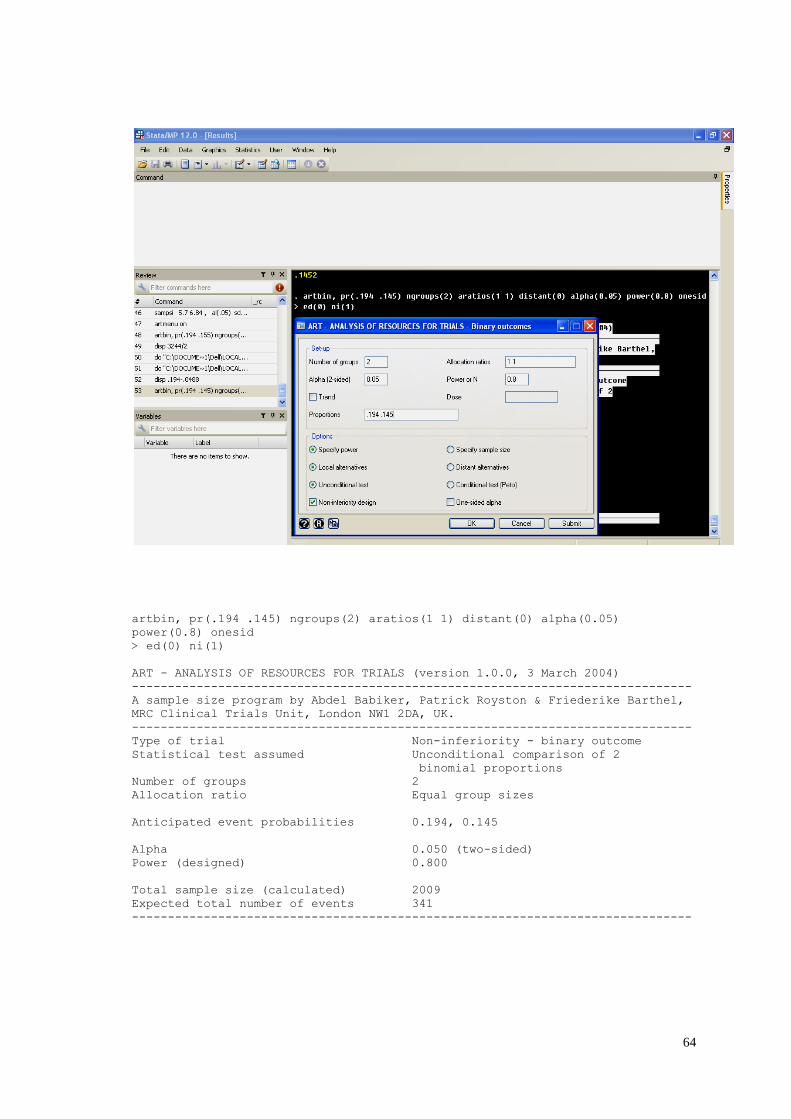
artmenu on
Once the menu is activated, we can use a command from a drop down menu via user\art\binary
outcomes. Information for number of groups, allocation ratio, alpha, power, and proportions need to
be filled in, see below. In addition, options for non-inferior design and one-sided test should be
selected. A sample size of 2009 subjects was required for this study.
64
artbin, pr(.194 .145) ngroups(2) aratios(1 1) distant(0) alpha(0.05)
power(0.8) onesid
> ed(0) ni(1)
ART - ANALYSIS OF RESOURCES FOR TRIALS (version 1.0.0, 3 March 2004)
------------------------------------------------------------------------------
A sample size program by Abdel Babiker, Patrick Royston & Friederike Barthel,
MRC Clinical Trials Unit, London NW1 2DA, UK.
------------------------------------------------------------------------------
Type of trial Non-inferiority - binary outcome
Statistical test assumed Unconditional comparison of 2
binomial proportions
Number of groups 2
Allocation ratio Equal group sizes
Anticipated event probabilities 0.194, 0.145
Alpha 0.050 (two-sided)
Power (designed) 0.800
Total sample size (calculated) 2009
Expected total number of events 341
------------------------------------------------------------------------------
65
ASSIGNMENT VI
1. A case-controlled study will be conducted to assess the association between diabetic
mellitus (DM) and cardiovascular diseases. The hypothesis is that patients with diabetes have
higher risk of cardiovascular events than non-diabetic patients. Previous literature reported that
the prevalence of diabetes in the general population was ~16%. The authors thought that an
odds ratio of at least 3 will have an impact on clinical practice.
a) Estimate sample size for this case-controlled study.
b) If the difference of diabetic prevalence between cases and controls is considered
instead of OR, by setting the size of difference = 10%, how many cases and controls would you
suggest?
c) If your colleague can conduct the study with only 100 subjects for each group, what
power will they come up with and how large is the difference which they will be able to detect?
Your colleagues have also asked you to write this calculation to add in a proposal.
2. A randomized controlled trial aims to test whether efficacy of ACE inhibitor is equivalent
to ARB in reno-protective effect. The outcome of interest is serum creatinine, in which mean
and its SD in type 2 diabetic patients who received ARB are 1.25 and 0.2, respectively. If a
difference of serum creatinine between the 2 drugs is ±0.05, it would be claimed as the 2 drugs
are clinically equivalent.
a) How many subjects will need to be enrolled to test this hypothesis,
b) Since ARB is more expensive than ACE inhibitor, what is your suggestion to
minimize the budget of their projects?
c) From their previous experiences of conducting clinical trials in their settings, a loss to
follow-up rate could reach to 25%. Justify the sample size according to loss to follow-up.
d) Writing a report for this part.


![Faculty of Science25/2/2563 Mail — opinter@mahidol.ac.th [POSTECH 2020 FALL] Call for Exchange Nomination Monica No (POSTECH) Mon 17/02/2020 07:16](https://img.pdfslide.net/doc/110x75/60985a1f7206ed2cd729e9c9/faculty-of-science-2522563-mail-a-opintermahidolacth-postech-2020-fall.jpg)