Embed Size (px)
Citation preview

Racial Preferences in Dating
Raymond Fisman, Sheena S. Iyengar, Emir Kamenica, & Itamar Simonson
First Draft: August 15, 2004 This Draft: June 28, 2006
Abstract
We examine racial preferences in dating using data from a Speed Dating experiment. In contrast to previous studies, our methodology allows us to directly observe individual decisions and thus easily infer whose preferences lead to racial segregation in romantic relationships. Moreover, the richness of our data allows us to identify many determinants of same race preferences. We find that females exhibit stronger racial preferences than males. We demonstrate that this gender difference is not due to different dating goals by men and women. Exogenously bringing attention to possible shared interests increases the willingness to date people from other races. The subject’s background, including the racial composition of the ZIP code where the subject grew up and the prevailing racial attitudes in the subject’s state of origin, strongly influence the desire to be with a partner of the same race. Older subjects and more physically attractive subjects exhibit weaker same race preferences.
__________________________________ *Fisman: Columbia University GSB. Uris 823, Columbia University, New York, NY 10027; email: [email protected]; tel: 212-854-9157; fax: 212-854-9895. Iyengar: Uris 714, Columbia University, New York, NY 10027; email: [email protected]; tel: 212-854-8308; fax: 212-316-9355. Kamenica: Harvard University Economics Department, Littauer Center, Cambridge, MA 02138; email: [email protected]; tel: 617-588-1439. Simonson: Graduate School of Business, Stanford University, Stanford, CA 94305-5015; email: [email protected]; Tel.: 650-725-8981; fax: 650-725-7979.

2
Inter-racial marriages in the United States are quite rare. For example, data from
the 5 percent sample of the 2000 Census reveals that among married blacks, 94% are
married to other blacks. Members of other races are also unlikely to marry outside of their
own group. In fact, even though under random matching 44% of all marriages would be
inter-racial,1 a mere 4% of marriages in the United States are between partners of different
race. However, this does not necessarily imply an underlying preference for spouses of the
same race: a final match (i.e., a marriage) is the outcome of a search process that involves
both finding and choosing a mate. Prior evidence across a range of disciplines reveals
extensive racial segregation in the United States, both geographic and social (see, for
example, Cutler, Glaeser, and Vigdor, 1999 and Massey, 2001). Inter-racial matches may
be rare, therefore, simply because members of different races interact relatively
infrequently. Rates of inter-racial marriage thus capture both preferences and socio-
geographic segregation. Identifying the separate roles of these two factors would enhance
our understanding of racial discrimination in this very important realm of human behavior.
Moreover, even if we knew the relative importance of preferences and segregation,
we might not know whose preferences drive the low rates of inter-racial marriage. For
example, suppose we observed an integrated community of whites and blacks with no
inter-racial marriages. This pattern would be consistent with a world where whites have a
strong preference for same race partners and blacks have none, but also consistent with the
world where whites are colorblind but blacks strongly dislike having a white marriage
partner. Similarly, the observed pattern would be consistent with either gender exhibiting a
strong same race preference. In order to get inside the black box of marital segregation we
need to observe decisions, not just final matches.2
Finally, we wish to know what drives racial preferences. Is it different interests, a
different sense of aesthetics, or some other factor? Does growing up in a neighborhood
populated with a particular race increase or decrease one’s romantic interest in members of
that race? Do prevailing racial attitudes in one’s hometown affect tolerance for partners of
a different race many years later? 1 We calculate this number using the overall populations in the United States, regardless of age. Alternative measures that restrict the calculation only to “marriageable” populations yield a similar figure. 2 In principle, one could estimate a structural model using data on marriages, but with this approach the results would be sensitive to functional form assumptions. Wong (2003) estimates a structural matching model using the PSID, but she does not address the issue of racial preferences.

3
In this paper, we study these issues through participants’ revealed preferences rather
than survey responses that served as the basis for earlier work. We study the effect of race
on mate selection by analyzing the choices of subjects in an experimental Speed Dating
service involving students from Columbia University graduate and professional schools.
Briefly, in our experimental paradigm subjects meet a number of potential mates for four
minutes each, and have the opportunity to accept or reject each partner.3 If both parties
desire a future meeting, then each receives the others’ email address the following day. We
emphasize that our design allows us to directly observe individual preferences of each
participant (i.e., their Yes/No decisions for each every partner). Further, during the event,
subjects rate their partners after each meeting, which helps us to get at the factors that
underlie same race preferences.4 Finally, we emphasize that our experiment takes place in a
realistic dating environment that provides strong assurance that the results are relevant
beyond the laboratory.
Our results are as follows. We observe a strong asymmetry across genders in racial
preferences: women of all races exhibit strong same race preferences, while men of no race
exhibit a statistically significant same race preference. Since older subjects (who are more
likely to attend the Speed Dating sessions in hope of starting a serious relationship)5 have a
weaker same race preference, this gender difference is unlikely to result from differential
dating goals between men and women. Our subjects do not find partners of the same race
more attractive, but do report significantly higher shared interests with partners of the same
race. However, the higher self-reported shared interests are capturing something different
than any of our objectively constructed proxies for shared interests. Moreover, in sessions
where subjects were asked to bring a favorite book or magazine, and thus where potential
shared interests were emphasized, racial preferences were weaker.
We also find that subjects’ backgrounds strongly influence their racial preferences.
First, we consider the effect of the prevailing attitudes toward inter-racial marriage in
subjects’ state of origin, based on responses to questions in the General Social Survey (for 3 Throughout the paper, we will refer to the person making the decision as subject and the person being decided upon as partner. When we wish to refer to both subjects and partners, we use the word participant. 4 In order to link our results on dating behavior to patterns of interracial marriage, we must assume that there is a correlation between characteristics that are desirable in a dating partner and characteristics that are desirable in a marriage partner. Sprecher and Regan (2002) and Stewart et al. (2000) both find a close concordance between attributes desired in dating and marriage partners, based on survey data. 5 As revealed in our pre-event survey, described below.

4
the subjects from the U.S.) and the World Value Survey (for non-U.S. subjects). Subjects
that come from intolerant places reveal stronger same race preferences. This is somewhat
surprising given the fact that our subjects are graduate students at Columbia University and
that many of them attended college away from home. We also consider the effect of early
exposure to other races and find that when there is a greater fraction of people of a
particular race in the ZIP code where the subject grew up, the subject’s willingness to date
someone from this group is lower. In other words, familiarity can decrease tolerance. This
result is unaffected by controlling for the average income in the ZIP code. Finally, we also
find that more physically attractive people care less about the race of the partner.
Our paper speaks directly to a broad literature in economics, psychology, and
particularly sociology on racial preferences in mate choice. Concurrent with our work,
Hitsch et al. (2005) provide the only other methodology for studying dating preferences
using actual decisions. They analyze email exchanges on a match-making website, and
report a broad set of findings on the determinants of dating preferences. Among their
findings is the existence of same race preferences, particularly for women. In a previous
paper (Fisman et al. 2006), we also mention the finding that women have stronger racial
preferences than men. However, our purpose here is not to merely document the existence
of racial preferences, but to understand their determinants. Thus, in this paper we consider
the heterogeneity of preferences across the different races, and much more importantly, we
examine which attributes induce stronger preference for the partner of a same race. We
thus begin the build a picture of the determinants of racial preferences.
Apart from these recent studies, existing research on inter-racial marriage and
dating relies exclusively on survey responses or population statistics; our results on gender
differences in particular are broadly consistent with these survey-based findings. For
example, Mills et al.’s (1995) survey suggests that both men and women hold negative
attitudes toward inter-racial relationships, but that women are significantly less accepting
of inter-racial romantic relationships than men are.6 Some earlier survey work also
attempts to document the determinants of racial preferences, but with results that are often
at odds with what we report here. For example, Mok (1999) reports a negative correlation
between own-race population density in respondents’ place of origin and the likelihood of
6 See Fujino (1997) and Fiebert et al. (2000) for additional work on gender differences in racial preference.
5
self-reported interracial dating. The contrast of these results with our findings highlights the
importance of our revealed preferences approach, since our approach allows us to
distinguish between exposure and preference. Yancey (2002) analyzes the demographic
correlates of self-reported interracial dating, and finds that age is negatively correlated with
interracial dating, but this could be due to differing levels of willingness to honestly reveal
interracial dating behavior across age groups. He also reports that respondents from the
American South are less likely to have dated inter-racially, which is consistent with our
findings on home state racism.
In the broad realm of racism in general, there is of course a vast literature on the
determinants of racial tolerance. The most relevant set of results for our study are those on
racism as a function of neighborhood integration. In particular, Wesley (1995) reports that
residential proximity to blacks is associated with greater racial prejudice.7 This association
is confirmed in our study.
The rest of the paper is structured as follows. Section 1 describes our data and
methodology. Section 2 describes our empirical results. Section 3 concludes.
1. Experimental Design
Our experimental design is based on meetings through Speed Dating, in which
participants engage in four-minute conversations to determine whether or not they are
interested in one another romantically. If both partners ‘accept’ then each is subsequently
provided with the other’s contact information to set up more leisurely dates in the future.
Three surveys, described below, were administered to the participants before, immediately
after, and 3 weeks after the event.
The main advantage of our design is that it gives us experimental control and yet
provides us with data on decisions made in a setting very similar to that which arises in the
real world. Speed Dating is a well established format in the United States, with eight
companies in 2004 devoted exclusively to this approach in New York City alone, in
addition to the many online match-making companies that offer Speed Dating as one of
their services. We made a special effort to ensure that our design creates a setting similar
7 In contrast, however, Welch et al. (2001) report that residents of integrated neighborhoods perceive a greater decline in racism over the previous decade than residents of more segregated neighborhoods.

6
to that provided by the private firms operating in this market.8 The evening's script was
based specifically on the Hurry Date format, the largest Speed Dating company in New
York.
Our subjects were drawn from students in graduate and professional schools at
Columbia University. Participants were recruited through a combination of mass e-mail
and fliers posted throughout the campus and handed out by research assistants. In order to
sign up for the Speed Dating events, interested students had to register at an online website
on which they reported their names and e-mail addresses and completed a pre-event
survey.9 Finally, for two of the sessions, the subjects were asked to bring along reading
materials: in the first of these, subjects were instructed as follows: “To add a little twist,
please bring your favorite magazine.” In the second case, subjects were instructed to bring
their “favorite piece of classic literature.”
Setting – The Speed Dating events were conducted in an enclosed room within a
popular bar/restaurant near the campus. The table arrangement, lighting, and type and
volume of music played were held constant across events. Rows of small square tables
were arranged with one chair on either side of each table.
Procedure – Speed Dating events were conducted over weekday evenings during
2002-2004; data from seventeen of these sessions are utilized in this study.10 In general,
two sessions were run in a given evening, with participants randomly distributed between
them.
Upon checking in, each participant was given a clipboard, pen, and nametag on
which only his or her ID number was written. Each clipboard included a scorecard with a
cover over it so that participants’ responses would remain confidential. The scorecard was
divided into columns in which participants indicated the ID number of each person they
met. Participants would then circle “yes” or “no” under the ID number to indicate whether
they wanted to see the other person again. Beneath the yes/no decision was a listing of the
8 The only important difference is that we did not serve alcohol. 9 This pre-event survey did include questions about racial preferences. We acknowledge that it would have been preferable to exclude such questions in order to avoid any possibility of articulation effects, but this is not a great concern given our focus on the determinants, rather than the level, of racial preferences. 10 We ran a total of twenty-one sessions; four have been omitted, one because we imposed a ‘budget set’ (i.e., maximum number of acceptances) on participants, and three because we were unable to attract sufficient participants.

7
six attributes on which the participant was to rate his or her partner on a 1-10 Likert scale:
Attractive; Sincere; Intelligent; Fun; Ambitious; Shared Interests.11
After all participants had arrived, two hosts instructed the participants to sit at the
two-person tables. The females were told to sit on one side of the tables, while the males
were seated across from them. Males were instructed to rotate from table to table, so that
by the end of the dating event they had rotated to all of the tables, meeting all of the
females.12 Each rotation consisted of four minutes during which the participants engaged
in conversation. After the four minutes, the Speed Dating hosts instructed the participants
to take one minute to fill out their scorecards for the person with whom they were just
speaking.
When all of the dating rounds were completed, the hosts concluded by letting
participant know that they would be sent a survey the following day, “You will be
receiving an email with a link for the follow-up survey. After you have filled it out, we
will send you an email with your match results.”
The morning after the Speed Dating event, participants were sent an e-mail
requesting that they complete the follow-up online questionnaire. Ninety-one percent (51
percent female, 49 percent male) of the Speed Dating participants completed this follow-up
questionnaire in order to obtain their matches. Upon receipt of their follow-up
questionnaire responses, participants were sent an e-mail informing them of their match
results.
Data Description
The main variable of interest is the Yes/No decision of subject i with respect to a
partner j, which we denote by Decisionij. We will initially examine gender differences in
same race preferences, and define the indicator variable Malei denoting whether the subject
is male.
11 A number of other responses, which we do not utilize in this paper, were also elicited from the subjects. For the complete survey, please see http://www2.gsb.columbia.edu/faculty/rfisman/Dating_Survey.pdf 12 This was the only asymmetry in the experimental treatment of men and women. While we would have preferred to have men and women alternate in rotating, we were advised against this by the owners of HurryDate. We believe this experimental asymmetry is unlikely to account for the observed gender differences in racial preference we report below.

8
We utilize the subjective ratings provided by the Speed Dating participants. We will
find it to be useful to control for the physical attractiveness of both subjects and partners. In
each case, we use the average of all attractiveness ratings received by a particular subject
(partner), and denote this by Attractivenessi (Attractivenessj). Additionally, since we will be
interested in the extent to which shared interests explain race preference, we will also use
subject i's shared interest rating for partner j, denoted by SelfReportedSharedInterestsij. For
both the attractiveness and shared interests ratings, values were rescaled to take on values
between zero and one in order to make them more readily comparable to the race variables.
We also define a number of race-related variables. First, the race of subject i is
denoted by Racei, and we define indicator variables denoting each of the four main race
classifications: Whitei, Blacki, Hispanici, and Asiani. The indicator variable Sameraceij
denotes that i and j are of the same race. For our Asian population, we would have liked to
differentiate between South Asians and East Asians. Unfortunately, however, we did not
allow for this distinction in our survey, though we did record the self-reported names and
places of origin of our subjects. The vast majority of Asian subjects were of East Asian
origin; we omit observations where the subject’s place of origin was in South Asia, or
where the subject’s name was clearly identifiable as South Asian. There were insufficient
South Asian subjects to include them as a separate category; therefore we omit them.13
We are interested in whether seriousness in dating objectives might be responsible
for differences in racial preferences. In the pre-event survey, we did ask the participants,
“What is your primary goal in participating in this event?” but since honest revelation is a
significant concern for such questions, we prefer to use self-reported Agei as a proxy for
seriousness.14
The pre-event survey additionally provides us with the information on the
participants’ ZIP Code in the place they grew up for those who were raised in the United
States. Additionally, we obtained information on the participants’ countries of birth.
For participants raised in the United States, we match the ZIP code to census racial
composition and income data in 1990. We choose this year as the closest estimate of the 13 If we do not omit South Asian subject, we observe weaker same race preferences for Asians, but no other results are affected. We also did not distinguish between white and black Hispanics and it is quite possible that Hispanics have stronger same race preferences than our results imply. 14 The results are qualitatively the same, though somewhat weaker, if we use the indicated intent in place of age.
9
formative years of our subjects, who had a median age of 11 in 1990. We define Incomei
as the log median income in i's ZIP Code in 1990, and construct a variable Fractionij that is
the fraction of the population in i's ZIP Code in 1990 that is of j’s race.
We additionally use state and country of origin to match subjects to data on racial
attitudes in their places of origin. Note that we do not have such data at the ZIP Code level.
For subjects that grew up in the United States, we use responses from the 1988-1991
General Social Survey (GSS) to the following question: “Do you think there should be laws
against marriages between (Negroes/Blacks/African-Americans) and whites?” to generate
the variable MarriageBan_GSSi. This variable reflects the fraction of respondents from the
subject’s state of origin that answered yes to this question.15 For subjects for whom no ZIP
Code was available, we used data from the 1990 World Values Survey (WVS). In this
survey, respondents were given a list of groups, including “People of a different race,” and
asked the following: “On this list are various groups of people. Could you please sort out
any that you would not like to have as neighbors?” We use this to construct
RacistNeighbors_WVSi which reflects, for the subject’s country of birth, the fraction of
survey respondents who reported that they would not want a neighbor of another race.
Unfortunately, the WVS did not have questions specifically on interracial marriage or
dating. MarriageBan_GSS and RacistNeighbors_WVS are both rescaled to have means of
zero and standard deviations of one for the full set of states and countries respectively.
We also use ZIP Code and country of birth information to generate measures of
similarity. For subject-partner pairs where both ZIP Codes are available, we generate the
following: (i) logDifferenceIncomeij, the log of the absolute value of the difference between
the median incomes of the ZIP Codes of the subject and partner; (ii) logDistanceZIPCodeij,
the log of the distance between the subject and partner’s ZIP Codes; and (iii)
SameRegionUSij, which denotes that both subject and partner come from the same census
region of the United States. Using country-level data, we also define SameRegionWorldij
which denotes that the subject and partner were born in the same region of the world.
We generate two additional measures of similarity based on participants’ survey
responses. First, subjects were asked to enter their field of study, which we used to generate
15 Results based on a variable based on GSS responses on a question relating to a family member marrying a black person were virtually identical; there was a much larger sample of respondents for the law-based variable we report above.
10
the aggregate classifications Business, Law, Service, and Academic, which was then used
to generate the indicator variable SameFieldij. Also, when registering online for the Speed
Dating event, subjects were asked to rate on a 1-10 Likert scale their interests in 17
activities (e.g., playing sports, music, hiking) derived from a comparable list utilized by
Match.com. We construct a measure of shared interests based on these responses, which is
the simple correlation of the responses of each subject-partner pairing
(CorrelationInterestsij).
Finally, in three of the sessions, we asked subjects to bring their favorite book or
magazine, with the intention of intensifying the role of shared interests in subjects’
decisions. The indicator variable Booki denotes whether the subject took part in one of
these sessions.
Table 1A provides descriptive statistics of our subjects. Where possible, we also
provide statistics on the overall population of students in graduate and professional schools
at Columbia University. In terms of race, our sample very closely mirrors the overall
population of Columbia graduate and professional students, though this does mean that we
have a relatively small number of black subjects, as noted above. Approximately 25 percent
of the subjects study business, 10 percent study law, 20 percent are in service areas, and 45
percent are pursuing an academic degree. This well approximates the distribution in the
Columbia graduate population as a whole, though business students are somewhat over-
represented. Finally, the majority (nearly three quarters) of our subjects grew up in North
America (i.e., the United States and Canada).
Table 1B provides summary statistics on the subject-partner level characteristics. Of
particular interest is that approximately 47 percent of all meetings were between
participants of the same race.
2. Results
A summary table of the fraction of Yeses, i.e., affirmative decisions, by subject-
partner race, along with the number of observations in each cell, is given in Tables 2A and
2B for females and males respectively. The diagonal terms are generally higher than the
corresponding fractions in the right-hand column, which gives tentative evidence of same
race preferences. Nonetheless, 47% of all matches in our data are inter-racial. While this
11
is significantly below the 53% that we would observe under random matching, it is still far
above the 4% of inter-racial marriages observed in the Census data. 16 Hence, despite the
fact that our subjects exhibit substantive racial preferences, they seem far more tolerant
than the society at large. This is unsurprising, given the characteristics of our subject pool.
First, our subjects are highly educated, and prior survey-based research finds that same race
preferences are negatively correlated with education. Second, our subjects have self-
selected into a dating event where they might expect to encounter potential partners of
different races.17
2.1 Gender Differences We begin by reporting separate regressions for each race and gender based on linear
probability models where we allow racial preferences to differ across all races, i.e., we
allow the off-diagonal terms in Table 2A and 2B to differ from one another. For example,
for white subjects, we will look at:
(1) Decisionij = αi + β1Blackj + β2Hispanicj + β3Asianj + εij
where αi is a subject fixed-effect, and we omit the race indicator variable for the subject’s
own race. We report these results in Table 3.
We first look at the decisions of female subjects. For all races except Asians, all the
coefficients on the race indicator variables are negative, indicating a same race preference.
For black and white subjects, these coefficients are jointly significantly different from zero
at the 1 percent level (p-value<0.01); for Hispanics, the joint significance is at the 10
percent level, with most of the effect derived from a significant (p<0.05) preference against
Asian males. For Asian subjects, no coefficient is significant. We can reject the
hypothesis of equal preference against partners of other races for white, black, and
16 Ideally, we would compare the figure 47% with the fraction of inter-racial dates, not marriages, but such data are not available. However, our finding in Section 2 that those who are looking for a serious relationship exhibit a weaker same race preference suggests that the comparison to 4% is still meaningful. 17 Subjects were not informed of the demographic composition of other Speed Dating participants. They were, however, told that they would be meeting other Columbia graduate students, so it is at least plausible that they would expect to encounter demographics representative of Columbia graduate students overall. This turned out to be the case for our sample, as illustrated in Table 1A.

12
Hispanic subjects, owing largely to the relatively large preference against Asian males by
all other races.
For male subjects the coefficients on racial preferences are predominantly negative
but are not jointly significant at 5% for any race. For white and black subjects, when
females and males are pooled and gender-race interactions included we find that the male
race coefficients are significantly closer to zero than the female race coefficients. In
analogous regressions for Asian and Hispanic subjects, the coefficients are of mixed signs
and generally insignificant. Thus overall, women exhibit much stronger racial preferences
than men.
One possible reason for this gender difference might be the different dating goals of
men and women. In particular, one might be concerned that women are more interested in
forming a relationship while men are more interested in casual sex and that race has greater
relevance for the former endeavor. However, in Subsection 2.4, we demonstrate that older
subjects (who are presumably more interested in relationships) exhibit substantially weaker
same race preferences. Thus, the observed difference seems to reflect a genuine disparity
in men and women’s willingness to be with a partner of a different race, rather than
differing goals.
2.2 The Role of Attractiveness Might the observed racial preferences arise from racially distinct notions of
attractiveness? We analyze the role of attractiveness in racial preferences by asking two
questions: (i) Do men and women find partners of the same race more attractive than
partners of other races, and (ii) Do partners of different races receive roughly the same
distribution of attractiveness ratings?
In order to study the first question, we run OLS regressions of the form
(2) Attractivenessji = αj + β1Blacki + β2Hispanici + β3Asiani + εij
suppressing the dummy for partner’s race. Note that in these regressions, the independent
variables are indicator variables for the race of the subject giving the ratings, whereas in all
other regressions, the independent variables indicate the race of the partner. Table 4

13
reports the results. We find that most coefficients are not significant, and in fact 10 out of
the 24 point estimates are positive. The only coefficients that are negative and individually
significant are Hispanic men’s ratings of Asian women, and white and Asian women’s
ratings of black men. Given the overall number of coefficients we estimate, however, these
three effects are likely to be spurious. Therefore, we conclude that a subject’s own race
does not influence the rating of a partner’s attractiveness. This finding gives us confidence
that we can meaningfully speak of ‘objective’ attractiveness and that average rating is a
reasonable proxy for it.
With this measure in hand, we can address the second question of whether different
races receive roughly the same distribution of attractiveness ratings. We do so by running
OLS regressions of the average attractiveness rating a partner receives on that partner’s
race. We run separate a regression for each gender, but pool together subjects of different
races for ease of exposition, since Table 4 suggests no systematic differences in ratings
based on a subject’s own race. The results are reported in Table 5, with white as the
omitted category. For male partners (column (1)), our main finding is that Asians generally
receive lower ratings than men of other races.18 In fact, when we run the regressions
separately for each race, we find that even Asian women find white, black, and Hispanic
men to be more attractive than Asian men.19 Given that Asian men were the group that
other races expressed strongest preference against, and that Asian women expressed the
least preference against other races, this finding suggests that attractiveness may play an
important role in the determination of racial preferences, especially those against Asian
men. We similarly find that for females, Asian partners are consistently rated as less
attractive (column (2)), though we also find that black females receive significantly lower
ratings relative to whites. As above, we find that when these regressions are run separately
for each race, even Asian men find white, black, and Hispanic women to be more attractive
than Asian women.
These results strongly suggest the need to control for attractiveness in our analysis
of the effect of race on decisions. The results of these regressions with this control are
18 One may worry that race may be correlated with field of study, which in turn may be correlated with attractiveness in our sample. We do not detect any systematic pattern in the relationship between field of study and race, however, and when we include fixed effects for the partner's field our results are unaffected. 19 Results of regressions separated by the race of the subject are available in the Online Appendix.

14
reported in Table 6. The main changes are that we now get a same race preference for
Asian women as well, and the preference against Asians declines for other races. Both of
these changes derive from the fact that our pool of Asian males generally received low
attractiveness ratings. Strikingly, we observe almost no heterogeneity in racial preferences
after physical attractiveness has been controlled for. In no case can we reject the equality
of race coefficients, and furthermore, no two coefficients are significantly different from
one another.
Motivated by these results, we collapse our race variables into a single Samerace
indicator variable that denotes whether a partner is of the same race as the subject. Further, we
pool the races together, and include partner race fixed effects in all regressions that follow.
This consolidation is prompted by the observation that, with the exception of black women, we
cannot reject the hypothesis of equal same race preferences across races. Finally, we find that
the results we report below on the determinants of racial preferences are virtually identical for
both males and females. That is, while we find that females’ same race preferences are much
stronger than for males on average, both genders exhibit similar within-gender correlates of
racial preferences. We thus pool females and males as well in what follows, simply controlling
for gender interacted with Samerace (results by gender are in the Online Appendix) where
appropriate. The precise specifications are given in each subsection below.
2.3 Racial Preferences and Shared Interests Previous research has identified a vast, and possibly increasing, cultural divide
between races in areas such as language and leisure activities. For example, the top ten TV
shows for blacks and whites have only a single show in common.20 Hence, greater shared
interest with partners of one’s own race immediately suggests itself as a potentially
important candidate as a determinant of racial preferences in dating. We consider
regressions of the form:
(3) Decisionij = αj + γj + β1Attractivenessj + β2Sameraceij
+ β3Sameraceij*Malei + β4SharedInterestsij + εij
20 See Fryer and Levitt (2004) for a broader discussion of the white-black cultural gap.
15
where γj is a fixed effect for the partner’s race and SharedInterests is a proxy for the shared
interests between the subject and the partner.
We first examine the role of SelfReportedSharedInterests. We find that subjects
report greater shared interests with partners of the same race, and as column (1) of Table 7
indicates, when we include SelfReportedSharedInterests as a control, the effect of race on
decisions is substantially reduced.
The interpretation of this result is somewhat problematic, however, particularly
given that the average attractiveness rating of the partner is highly predictive of
SelfReportedSharedInterests. This strongly suggests that SelfReportedSharedInterests is
capturing more than just shared interests. In the other columns of Table 8, we demonstrate
that more objective measures of shared interests leave the same race coefficient intact.
Moreover, as column (8) in Table 7 shows, in the sessions where each subject brought his
or her favorite book or magazine, same race preferences were lower, as indicated by the
negative coefficient on the interaction term Samerace*Book. Since the ability to compare
reading preferences should make shared interests more salient, this result provides further
evidence that shared interests do not account for much of the observed racial preferences.
This result is also important in light of discussions on efforts to promote inter-racial
interactions, as it suggests exposure to the views of other races may be useful in attenuating
racial preferences.
2.4 Racial Preferences and Subject’s Attributes Much of the earlier literature on racial attitudes on dating (and on dating in general)
focuses on individuals’ personal characteristics as determinants of racial preferences. Here,
we bring our revealed preference methodology to bear on this question.
We consider regressions of the following form:
(4) Decisionij = αj + γj + β1Attractivenessj + β2Sameraceij
+ β3Sameraceij*Malei + β4Sameraceij*Xij + εij

16
where Xij is a variable that may affect racial preferences and γj is a fixed effect for the
partner’s race.
First, we analyze the effects of upbringing on racial preferences, as emphasized by
much of the earlier survey-based literature. A natural starting point for examining the
effects of background is to consider the role of the prevailing attitudes on race in subjects’
place of origin. For subjects that grew up in the United States, we use the intensity of
support for a ban on inter-racial marriage in the subject’s home state (MarriageBan_GSS).
For subjects who did not grow up in the United States, we use the variable
RacistNeighbors_WVS, which reflects, for the subject’s country of birth, the fraction of
survey respondents in the 1990 World Values Survey (WVS) who reported that they would
not want a neighbor of another race
Columns (1) and (2) of Table 8 show the results for each of the survey-based
variables (MarriageBan_GSS and RacistNeighbors_WVS) interacted with Samerace. In
both cases, the interaction is significant and positive, indicating stronger racial preferences
for subjects from backgrounds with less tolerance for inter-racial mixing. This highlights
the persistence of background in dictating racial preferences in dating (and potential
attitudes on race generally), and is all the more surprising given that the sample consists of
graduate students studying at Columbia University who may have been away from home
for some time. In column (3) we show results based on a variable, HomeRacism that takes
the value of MarriageBan_GSS for subjects that grew up in the U.S. and the value of
RacistNeighbors_WVS otherwise. For this pooled sample, we similarly obtain a positive
and significant interaction of home state tolerance and the same race indicator variable.
We additionally examine whether growing up in a neighborhood with people of a
different race changes the willingness to date someone from that race. Theoretically, the
relationship is ambiguous – familiarity may breed understanding, but may also be the
source of racial tension. To examine this effect, we interact Samerace with Fraction, which
denotes the fraction of the population in subject i's ZIP code that is of partner j’s race.
Column (4) of Table 8 shows that, on average, early familiarity with a race decreases
tolerance, though the effect is only marginally significant (p=0.09). This surprising effect
of exposure is consistent with the work of Welch (1995), though as noted in the
introduction other studies find the opposite effect (see, for example, Mok, 1999). Since
17
income differs systematically with the racial composition of neighborhoods, one potential
explanation is that subjects who grew up in predominantly minority neighborhoods form
negative associations with other races. We find, however, that these effects are not affected
by including the interaction of average income by ZIP code with the same race indicator
variable. Interestingly, as demonstrated in column (5) of Table 8, we also find that income
of ZIP code interacted with the race indicator variable is quite close to zero, implying that
economic background is uncorrelated with same race preferences.21
Finally, we turn to a set of additional basic subject attributes and examine whether
they are correlated with racial preferences. We first examine the role of age. As column (1)
of Table 9 indicates, older subjects discriminate less on the basis of race. The effect is
quite strong and statistically significant (p<0.01). This is consistent with earlier work
suggesting that older persons have a broader field of eligible partners (e.g., South, 1991).
Second, we examine the effect of subject’s attractiveness. Strikingly, more attractive
people have much weaker same race preferences. Finally, in column (3) we examine
whether subjects pursuing less liberal-minded careers demonstrate stronger racial
preferences, by looking at the interaction of Samerace with an indicator variable denoting
whether the subject was enrolled in a business or law program (BusinessOrLawi); this
interaction term is not significant.
2.6 Robustness Note that even though we have a large number of meetings, we have a small
number of meetings between subjects of certain races. For this reason, the standard errors
implied by the regression framework may be misleading. The standard errors from the
regressions are primarily problematic for black subjects, due to the paucity of their same
race meetings. We therefore also calculate the significance of blacks’ same race
preferences using an approach that does not invoke large sample theory. Let qi be the
empirical fraction of non-black partners to whom black subject i says Yes. Under the null
hypothesis of no same race preference, we assume that this is also the probability that
21 These results are consistent with Yancey (2002). In his survey data, income does not predict inter-racial dating, and having lived in inter-racial neighborhoods is correlated with inter-racial dating for whites and blacks, but not for Hispanics and Asians.
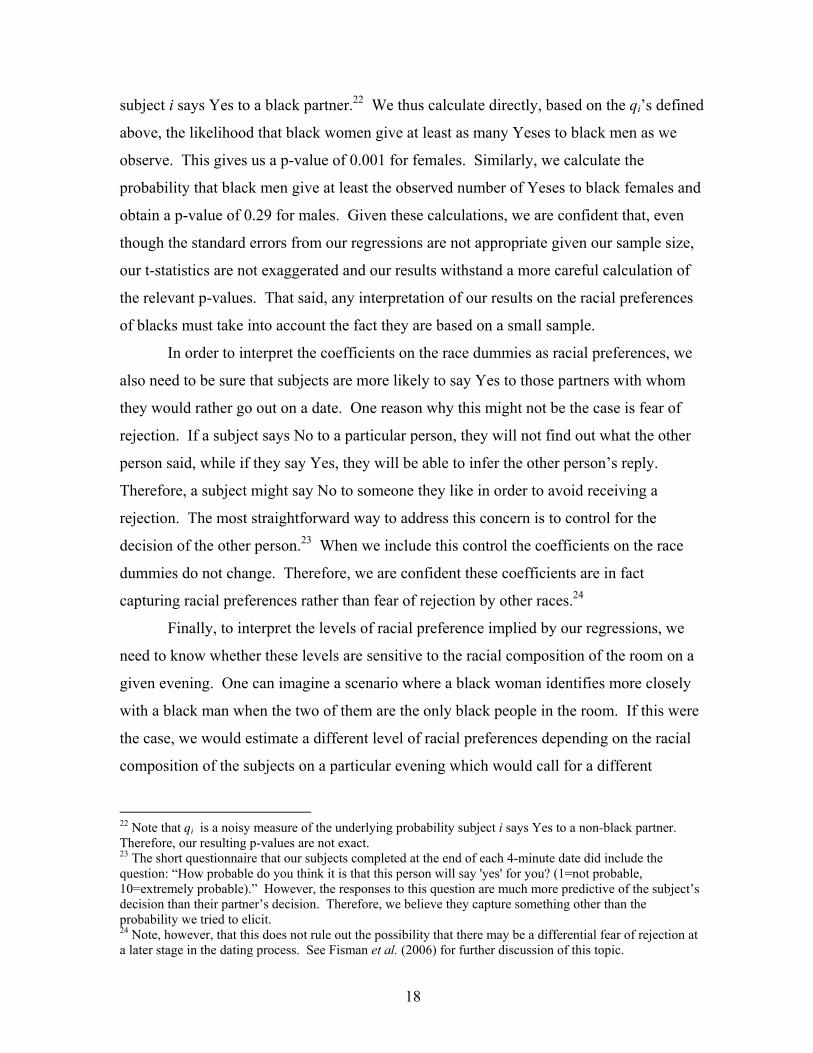
18
subject i says Yes to a black partner.22 We thus calculate directly, based on the qi’s defined
above, the likelihood that black women give at least as many Yeses to black men as we
observe. This gives us a p-value of 0.001 for females. Similarly, we calculate the
probability that black men give at least the observed number of Yeses to black females and
obtain a p-value of 0.29 for males. Given these calculations, we are confident that, even
though the standard errors from our regressions are not appropriate given our sample size,
our t-statistics are not exaggerated and our results withstand a more careful calculation of
the relevant p-values. That said, any interpretation of our results on the racial preferences
of blacks must take into account the fact they are based on a small sample.
In order to interpret the coefficients on the race dummies as racial preferences, we
also need to be sure that subjects are more likely to say Yes to those partners with whom
they would rather go out on a date. One reason why this might not be the case is fear of
rejection. If a subject says No to a particular person, they will not find out what the other
person said, while if they say Yes, they will be able to infer the other person’s reply.
Therefore, a subject might say No to someone they like in order to avoid receiving a
rejection. The most straightforward way to address this concern is to control for the
decision of the other person.23 When we include this control the coefficients on the race
dummies do not change. Therefore, we are confident these coefficients are in fact
capturing racial preferences rather than fear of rejection by other races.24
Finally, to interpret the levels of racial preference implied by our regressions, we
need to know whether these levels are sensitive to the racial composition of the room on a
given evening. One can imagine a scenario where a black woman identifies more closely
with a black man when the two of them are the only black people in the room. If this were
the case, we would estimate a different level of racial preferences depending on the racial
composition of the subjects on a particular evening which would call for a different
22 Note that qi is a noisy measure of the underlying probability subject i says Yes to a non-black partner. Therefore, our resulting p-values are not exact. 23 The short questionnaire that our subjects completed at the end of each 4-minute date did include the question: “How probable do you think it is that this person will say 'yes' for you? (1=not probable, 10=extremely probable).” However, the responses to this question are much more predictive of the subject’s decision than their partner’s decision. Therefore, we believe they capture something other than the probability we tried to elicit. 24 Note, however, that this does not rule out the possibility that there may be a differential fear of rejection at a later stage in the dating process. See Fisman et al. (2006) for further discussion of this topic.

19
interpretation of our estimates. Unfortunately, we have insufficient variation in the number
of black and Hispanic subjects across evenings to analyze the effect of racial composition
on their decisions, but we do have enough variation in the number of Asian subjects and are
able to reject the presence of any such effects for Asians.
3. Conclusion Our results indicate that even in a population of relatively progressive individuals
who have self-selected into participation in a multi-cultural Speed Dating event we observe
strong racial preferences. Therefore, preferences are likely to play at least some role in
explaining the low rates of inter-racial marriages in the United States today.
Recall, however, that even though the race of the partner strongly influences
individual decisions, 47% of all matches in our data are inter-racial. Schelling’s (1971)
model of dynamic segregation shows that even an extremely mild preference for neighbors
of one’s own race may lead to completely segregated neighborhoods. In our dating market,
however, we encounter a different relationship between micromotives and macrobehavior:
our subjects have a strong preference for partners of their own race, yet the overall level of
the resulting segregation is quite small.25
Our study provides an important methodological innovation for understanding the
nature of racial preferences in mate selection. In contrast to observational studies, our
experimental approach allows for the direct observation of individual preferences, and in
contrast to survey-based evidence, the decisions our subjects make have real consequences.
Given that our population is one where we might least expect to see racial preferences, the
effects we report are surprisingly large.
Our results suggest a number of directions for future research. First, we report
striking findings on the importance of background, both in terms of prevailing racial
attitudes and racial diversity in one’s place of origin, in affecting racial preferences. This
work could be extended to include more refined measures of racial characteristics of place
of origin, and other background attributes such as family characteristics. The strength and
consistency of our results on age and physical attractiveness also provide some intriguing
25 The basic reason why residential and marital segregation are different in this regard is straightforward: the positive feedback process that underlies Schelling’s result is not applicable to matching markets.

20
hints as to the determinants of tolerance across individuals and over the life cycle, and
future work may try to better understand the factors driving these findings.

21
References
Cutler, David, Edward Glaeser and Jacob Vigdor (1999) “The Rise and Decline of the American Ghetto,” Journal of Political Economy 107:455-506.
Fiebert, Martin S., Holly Karamol, and Margo Kasdan (2000) “Interracial Dating: Attitudes and Experience Among American College Students in California,” Psychological Report, 87:1059-1064.
Fisman, Raymond, Sheena Iyengar, Emir Kamenica, and Itamar Simonson (2004) “Searching for a Mate: Theory and Experimental Evidence,” Working Paper.
Fryer, Roland, and Steven Levitt (2004). “The Causes and Consequences of Distinctively Black Names,” Quarterly Journal of Economics 119, 3:767-805.
Fujino, Diane C. (1997) “The Rates, Patterns and Reasons for Forming Heterosexual Interracial Dating Relationships Among Asian Americans,” Journal of Social and Personal Relationships, 14(6):809-828.
Hitsch, Gunter J., Dan Ariely, and Ali Hortacsu (2004) “What Makes You Click: An Empirical Analysis of Online Dating,” Working Paper
Massey, Douglas (2001) “Residential Segregation and Neighborhood Conditions in U.S. Metropolitan Areas,” in America Becoming: Racial Trends and Their Consequences, Vol. 1, 391-434. Washington DC: The National Academies Press.
Mills, Jon K., Jennifer Daly, Amy Longmore, and Gina Kilbridge (1995) “A Note on Family Acceptance Involving Interracial Friendships and Romantic Relationships,” The Journal of Psychology, 129(3): 349-351.
Mok, Teresa A. (1999) “Asian American Dating: Important Factors in Partner Choice,” Cultural Diversity and Ethnic Minority Psychology, 5(2):103-117.
Schelling, Thomas C. (1971) “Dynamic Models of Segregation,” Journal of Mathematical Sociology. 1:143-186.
South, Scott J. (1991), “Sociodemographic Differentials in Mate Selection Preferences,” Journal of Marriage and Family, 53 (November): 928-40.
Sprecher, S., & Regan, P. C.(2002) “Liking some things (in some people) more than others: Partner preferences in romantic relationships and friendships.” Journal of Social and Personal Relationships, 19, 463-481.
Stewart, Stephanie, Heather Stinnett, and Lawrence B. Rosenfeld, “Sex Di¤erences in Desired Characteristics of Short-Term and Long-Term Relationship Partners,” Journal of Social and Personal Relationships, XVII (2000), 843: 853.

22
Welch, Susan, Timothy Bledsoe, Lee Sigelman, and Michael Combs. Race and Place: Race Relations in an American City. Cambridge: 2001.
Wesley G., “Crime and the Racial Fears of White Americans.” Annals of the American Academy of Political and Social Science, Vol. 539 (May, 1995) , pp. 59-71
Wong, Linda Y. (2003) “Structural Estimation of Marriage Models,” Journal of Labor Economics. 21, 3: 699-729.
Yancey, George (2002) “Who Interracially Dates: An Examination of the Characteristics of Those who Have Interracially Dated,” Journal of Comparative Family Studies 33(2): 179-190.

Number of Participants Percentage
Columbia Graduate Population Percentage
A. Race of ParticipantWhite 262 63.59% 3978 68.67%Black 25 6.07% 424 7.32%Hispanic 40 9.71% 416 7.18%Asian 85 20.63% 975 16.83%Total 412 5793B. Field of StudyBusiness 95 24.48% 1925 18.21%Law 40 10.31% 1530 14.48%Service 78 20.10% 2161 20.45%Academic 175 45.10% 4953 46.86%Total 388 10569C. Region of OriginNorth America 257 74.28%Western Europe 31 8.96%Eastern Europe 7 2.02%Central Asia 6 1.73%Middle East 4 1.16%East Asia 28 8.09%Latin America 12 3.47%Africa 1 0.29%Total 346
Descriptive Statistics of ParticipantsTABLE 1A
Notes: Statistics for the Columbia graduate student population reflect total (part-time and full-time) enrolment, and are taken from the Statistical Abstract of Columbia University 2004 , available at http://www.columbia.edu/cu/opir/abstract/enrollment_fte_2004.html. No data are available on students' countries of origin.
Mean Std. Dev. Min Max ObsIncome ($1000) 45.768 18.522 8.607 122.978 291Marriage Ban GSS -0.488 0.629 -2.649 1.708 286Racist Neighbor WVS -0.426 0.705 -1.137 3.365 82Age 26.229 3.544 19 42 410Attractiveness 0.624 0.119 0.280 0.869 412
Same Race 0.468 0.499 0 1 5998Shared Interests 0.546 0.216 0 1 5181Correlation Interests 0.195 0.307 -0.828 0.911 5966Same Region US 0.363 0.481 0 1 3088Same Region World 0.535 0.499 0 1 4870Same Field 0.321 0.467 0 1 5350
Summary Statistics
Notes: Income is the median income (in $1000) of the partner's zip code in 1990, based on United States census data. Marriage Ban GSS is the fraction of respondents to the General Social Survey, from the subject's state of origin, who responded affirmatively to the question, "Do you think there should be laws against marriages between (Negroes/Blacks/African-Americans) and whites?" Racist Neighbor WVS is the fraction of respondents in the World Values Survey, from the subject's country of birth, who did not wish to have a neighbor of a different race. Age is the self-reported age of the participant. Attractiveness is the average rating of the partner by the subjects he or she meets. Same Race is an indicator variable denoting that the subject and the partner are of the same race. Shared Interests is the level of shared interests self-reported by the subject. Correlation Interests is the correlation of the stated list of interests from the pre-event survey. Same Region US is an indicator variable denoting that the subject and partner were born in the same census region of the United States. Same Region World is an
TABLE 1B
indicator variable denoting that the subject and the partner were born in the same part of the world as grouped in Table 1A. Same Field is an indicator variable denoting that the subject and partner are in the same area of study as grouped in Table 1A. For Same Race, Same Field, and Same Region the level of observation is a subject-partner meeting. For Income, the level of observation is ZIP Code. For Marriage Ban GSS the level of observation is state. For Racist Neighbor WVS the level of observation is country. For Age and Attractiveness the level of observation is subject.
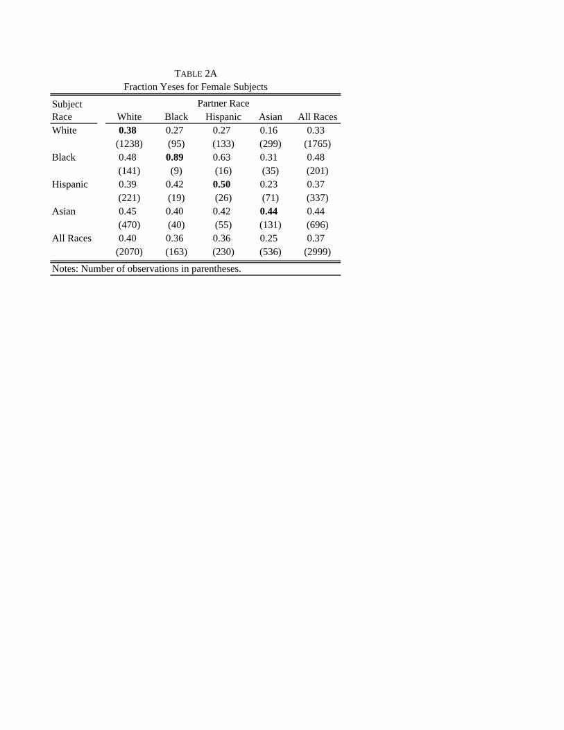
White Black Hispanic Asian All RacesWhite 0.38 0.27 0.27 0.16 0.33
(1238) (95) (133) (299) (1765)Black 0.48 0.89 0.63 0.31 0.48
(141) (9) (16) (35) (201)Hispanic 0.39 0.42 0.50 0.23 0.37
(221) (19) (26) (71) (337)Asian 0.45 0.40 0.42 0.44 0.44
(470) (40) (55) (131) (696)All Races 0.40 0.36 0.36 0.25 0.37
(2070) (163) (230) (536) (2999)
TABLE 2AFraction Yeses for Female Subjects
Partner Race
Notes: Number of observations in parentheses.
Subject Race

White Black Hispanic Asian All RacesWhite 0.49 0.41 0.50 0.35 0.46
(1238) (141) (221) (470) (2070)Black 0.59 0.67 0.63 0.43 0.56
(95) (9) (19) (40) (163)Hispanic 0.49 0.38 0.46 0.29 0.43
(133) (16) (26) (55) (230)Asian 0.53 0.37 0.38 0.47 0.48
(299) (35) (71) (131) (536)All Races 0.50 0.41 0.48 0.37 0.46
(1765) (201) (337) (696) (2999)
Notes: Number of observations in parentheses.
Subject Race
TABLE 2BFraction Yeses for Male Subjects
Partner Race

(1) (2) (3) (4) (5) (6) (7) (8)White -0.458 0.000 0.001 -0.077 -0.023 0.027
(0.162) (0.094) (0.054) (0.191) (0.125) (0.047)Black -0.104 -0.029 -0.027 -0.123 -0.209 -0.181
(0.060) (0.173) (0.071) (0.069) (0.187) (0.104)Hispanic -0.124 -0.374 0.007 0.040 -0.059 -0.077
(0.051) (0.195) (0.095) (0.060) (0.235) (0.060)Asian -0.243 -0.611 -0.224 -0.061 -0.275 -0.188
(0.034) (0.170) (0.111) (0.046) (0.199) (0.132)
Gender of subjectRace of subject White Black Hispanic Asian White Black Hispanic Asian
F-Test, Joint Sig. 0.00 0.00 0.10 0.97 0.15 0.11 0.16 0.08F-Test, Equality 0.02 0.06 0.01 0.89 0.15 0.06 0.10 0.04Observations 1765 201 337 696 2070 163 230 536R-squared 0.25 0.30 0.24 0.30 0.29 0.30 0.15 0.42
TABLE 3
Linear Probability Model. Robust standard errors in parentheses, clustered by partner. The dependent variable in all regressions is Decision, an indicator variable that takes on a value of one if a subject desired contact information for a partner. All regressions include subject fixed effects, and all observations are weighted by the inverse of the number of observation per subject.
Racial Preferences in Dating Decisions
Female Male

(1) (2) (3) (4) (5) (6) (7) (8)White -0.061 0.003 -0.021 -0.108 0.023 -0.037
(0.075) (0.053) (0.027) (0.045) (0.066) (0.023)Black 0.008 0.051 -0.028 0.061 0.12 0.026
(0.025) (0.071) (0.039) (0.027) (0.086) (0.054)Hispanic -0.058 -0.13 -0.128 0.001 -0.098 -0.04
(0.044) (0.086) (0.046) (0.021) (0.057) (0.046)Asian -0.03 -0.121 -0.007 0.012 -0.126 0.013
(0.021) (0.078) (0.058) (0.025) (0.054) (0.070)
Gender of PartnerRace of Partner White Black Hispanic Asian White Black Hispanic Asian
Observations 1469 171 201 420 1224 143 132 410R-squared 0.33 0.43 0.37 0.47 0.42 0.52 0.3 0.49
OLS. Robust standard errors in parentheses, clustered by partner. The dependent variable in all regressions is the average rating of the partner's attractiveness. All regressions include partner fixed effects, and all observations are weighted by the inverse of the number of observation per partner. Note that in these regressions, the independent variables are indicator variables for the race of the subjects giving the ratings, whereas in other tables, the independent variables indicate the race of the partner.
TABLE 4Effect of Subject's Race on Subjects' Attractiveness Ratings of Partners
Female Male

(1) (2) Black 0.007 -0.084
(0.037) (0.035)Hispanic -0.036 0.011
(0.027) (0.030)Asian -0.130 -0.061
(0.021) (0.020)
Gender of Subject Female MaleObservations 2535 2613R-squared 0.20 0.25
TABLE 5Effect of Partner's Race on Subjects' Attractiveness
Ratings of Partners
OLS. Robust standard errors in parentheses, clustered by partner. The dependent variable in all regressions is the average rating of the partner's attractiveness. All regressions include partner fixed effects, and all observations are weighted by the inverse of the number of observation per partner. Note that in these regressions, the independent variables are indicator variables for the race of the partner receiving the rating, whereas in the previous table, the independent variables indicate the race of the subject.

(1) (2) (3) (4) (5) (6) (7) (8)White -0.418 -0.059 -0.144 -0.200 0.010 -0.033
(0.113) (0.068) (0.046) (0.129) (0.088) (0.042)Black -0.118 -0.076 -0.204 0.011 0.046 -0.124
(0.045) (0.122) (0.076) (0.049) (0.134) (0.091)Hispanic -0.085 -0.336 -0.126 0.010 -0.245 -0.139
(0.032) (0.148) (0.076) (0.030) (0.146) (0.055)Asian -0.079 -0.420 -0.096 0.037 -0.211 -0.030
(0.028) (0.131) (0.078) (0.033) (0.140) (0.095)Attractiveness 1.300 1.360 1.560 1.340 1.650 2.150 1.920 1.030
(0.090) (0.220) (0.200) (0.140) (0.110) (0.250) (0.260) (0.150)
Gender of subjectRace of subject White Black Hispanic Asian White Black Hispanic Asian
F-Test, Joint Sig. 0.00 0.00 0.67 0.01 0.71 0.40 0.93 0.11F-Test, Equality 0.72 0.71 0.83 0.63 0.81 0.86 0.79 0.06Observations 1765 201 337 696 2070 163 230 536R-squared 0.35 0.42 0.38 0.40 0.43 0.53 0.32 0.47
Linear Probability Model. Robust standard errors in parentheses, clustered by partner. The dependent variable in all regressions is Decision, an indicator variable that takes on a value of one if a subject desired contact information for a partner. All regressions include subject fixed effects, and all observations are weighted by the inverse of the number of observation per subject.
TABLE 6
Female Male
Racial Preferences in Dating Decisions – Effect of Attractiveness

(1) (2) (3) (4) (5) (6) (7) (8)Same Race 0.055 0.103 0.106 0.121 0.121 0.121 0.105 0.115
(0.020) (0.020) (0.022) (0.029) (0.029) (0.029) (0.023) (0.021)Shared Interests 0.767
(0.042)Correlation Interests 0.043
(0.022)Same Field 0.025
(0.015)log(Distance Zip Code) 0.001
(0.008)log(Difference in Income) 0.044
(0.027)Same Region US 0.017
(0.017)Same Region World 0.044
(0.018)Book * Same Race -0.060
(0.033)Male * Same Race -0.061 -0.093 -0.086 -0.091 -0.092 -0.090 -0.093 -0.092
(0.028) (0.027) (0.029) (0.040) (0.040) (0.040) (0.031) (0.026)Attractiveness 1.325 1.615 1.630 1.654 1.658 1.654 1.623 1.615
(0.069) (0.067) (0.069) (0.091) (0.090) (0.090) (0.074) (0.067)
Observations 5181 5966 5350 3088 3088 3088 4870 5998R-squared 0.49 0.40 0.40 0.42 0.42 0.42 0.41 0.40
TABLE 7
Linear Probability Model. Robust standard errors in parentheses, clustered by partner. The dependent variable in all regressions is Decision, an indicator variable that takes on a value of one if a subject desired contact information for a partner. All regressions include subject fixed effects, and all observations are weighted by the inverse of the number of observation per subject. Same Race is an indicator variable denoting that subject and partner are of the same race. Shared Interests is subject's report of shared interests with the partner at the Speed Dating session. Correlation Interests is the correlation of subject's and partner's indicated interests from the pre-event survey. Same Field is an indicator variable denoting that subject and partner are in the same field of study as grouped in Table 1A. log(Distance Zip Code) is the log of distance in miles between the ZIP Codes where the subject and the partner grew up, while log(Difference in Income) is the log of the absolute value of the difference between the median incomes of the ZIP Codes of the subject and partner. Same Region US and Same Region World are indicator variables for whether the subject and partner are from the same
The Role of Shared Interets
census region of the United States or from the same part of the world as grouped in Table 1A. Book is an indicator variable denoting whether the participants were asked to bring their favorite book or magazine to the Speed Dating session.

(1) (2) (3) (4) (5)Same Race 0.146 0.046 0.130 0.088 0.201
(0.025) (0.087) (0.024) (0.028) (0.382)Marriage Ban GSS * Same Race 0.087
(0.024)Racist Neighbors WVS * Same Race 0.053
(0.028)HomeRacism * Same Race 0.075
(0.023)Fraction -0.110
(0.069)Fraction * Same Race 0.208
(0.124)log(Income) * Same Race -0.009
(0.036)Born in USA * Same Race
Male * Same Race -0.047 -0.040 -0.054 -0.067 -0.050(0.026) (0.100) (0.024) (0.031) (0.031)
Attractiveness 0.159 0.176 0.161 0.159 0.160(0.010) (0.016) (0.009) (0.007) (0.008)
Observations 4218 718 4936 4170 4288R-squared 0.39 0.36 0.39 0.40 0.39
The Role of Background
Linear Probability Model. Robust standard errors in parentheses, clustered by partner. All regressions include subject fixed effects, and all observations are weighted by the inverse of the number of observation per subject. Same Race is an indicator variable denoting that subject and partner are of the same race. Marriage Ban GSS is the fraction of respondents to the General Social Survey, from the subject's state of origin, who responded affirmatively to the question, "Do you think there should be laws against marriages between (Negroes/Blacks/African-Americans) and whites?" Racist Neighbor WVS is the fraction of respondents in the World Values Survey, from the subject's country of birth, who did not wish to have a neighbor of a different race. Home Racism is a variable that takes the value of Marriage Ban GSS for subjects who grew up in the United States and the value of Racist Neighbor WVS otherwise. Fraction is that is the fraction of the population in i's ZIP Code in 1990 that is of j’s race. log(Income) is the log of median income in subject's ZIP Code in 1990.
TABLE 8

(1) (2) (3)Same Race 0.331 1.071 0.105
(0.077) (0.350) (0.022)Own Attractiveness * Same Race -0.350
(0.112)log(Age) * Same Race -0.297
(0.108)Business or Law * Same Race -0.010
(0.030)Male * Same Race -0.119 -0.092 -0.072
(0.028) (0.027) (0.028)Attractiveness 1.612 1.614 1.600
(0.067) (0.067) (0.067)Observations 5998 5970 5613R-squared 0.40 0.40 0.40
Additional Correlates of Racial Preferences
Linear Probability Model. Robust standard errors in parentheses, clustered by partner. All regressions include subject fixed effects, and all observations are weighted by the inverse of the number of observation per subject. Same Race is an indicator variable denoting that subject and partner are of the same race. Own Attractiveness is the subject's average attractiveness rating. log(Age) is the log of the subject's age. Business or Law is an indicator variable denoting whether the subject's field of study is busineess or law.
TABLE 9