Radar Detection Performance Using Design of Experiments – Case Study

Scientia Prudentia et Valor

DISTRIBUTION STATEMENT A: Approved for public release; distribution is unlimited.

Luis A. Cortes, P.E.Darryl Ahner, P.E., Ph.D.

OSD STAT COEwww.AFIT.edu/STAT

937-255-3636 x 4736

Scientia Prudentia et Valor

This case study is an application of experimental design to the test and evaluation of surface radars.

It builds upon work done by the Naval Surface Warfare Center, Corona Division.

We look back into a test that was considered a landmark in M&S-based acquisition and contrast the way one objective was evaluated to the way it could have been evaluated with experimental design.

In the process, we explore the attributes of a well designed test and demonstrate the utility of experimental design for planning, designing, executing, and analyzing a test.

What can we learn from the data? What could we have done differently? What can we do different next time?

Bottom Line Up Front

2

An experimental design approach contributes to making the test more robust, efficient, and cost effective.

Scientia Prudentia et Valor

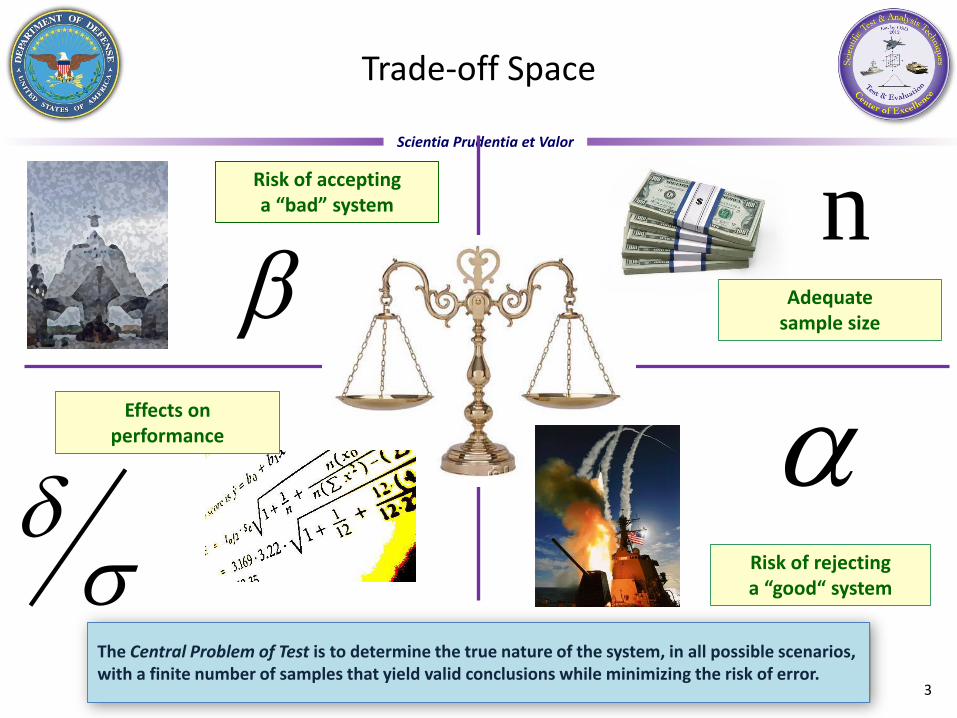
n

The Central Problem of Test is to determine the true nature of the system, in all possible scenarios, with a finite number of samples that yield valid conclusions while minimizing the risk of error.

Risk of accepting a “bad” system

Risk of rejectinga “good“ system

Effects on performance

3

Adequate sample size

Trade-off Space

Scientia Prudentia et Valor

An accredited federation of robust models and simulations replicated the at-sea conditions

Test events

80 hrs total test time

18 hrs of manned aircraft raids

110 electronic attack (EA) techniques

1900 simulated Anti Ship Cruise Missiles

Test Background

Test Operations

Evaluate detection performance for a class of threat representative targets*

Factors involved

Three target factors - A, B, F

Two environmental factors - C, D

One system factor - E

Test strategy

96 possible treatments

30 samples per treatment required

2880 total runs required

96 hrs of test required-not enough time!

670 runs conducted

Assessment criteria - Pass/Fail

One Objective

*Other objectives are beyond the scope of this brief; however, similar lessons apply.

4

Sacrificed statistical confidence due to test time limitations.

Had an informal criteria for selecting test runs.

Analysis limited to pass/fail.

Scientia Prudentia et Valor

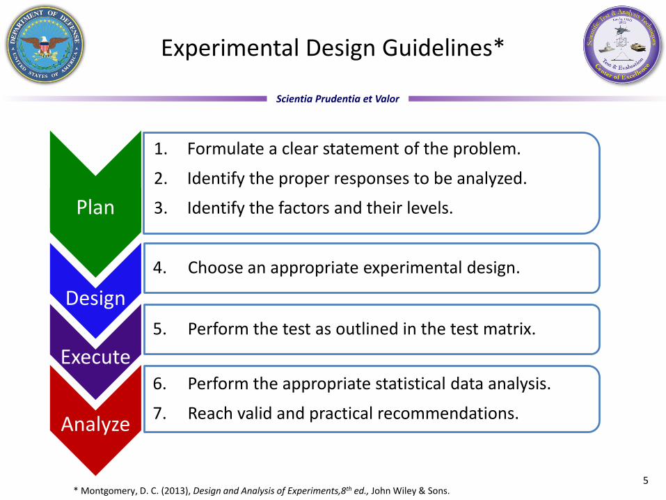
Experimental Design Guidelines*

Plan

1. Formulate a clear statement of the problem.

2. Identify the proper responses to be analyzed.

3. Identify the factors and their levels.

Design

4. Choose an appropriate experimental design.

Execute

5. Perform the test as outlined in the test matrix.

Analyze

6. Perform the appropriate statistical data analysis.

7. Reach valid and practical recommendations.

Execute

* Montgomery, D. C. (2013), Design and Analysis of Experiments,8th ed., John Wiley & Sons.5

Scientia Prudentia et Valor

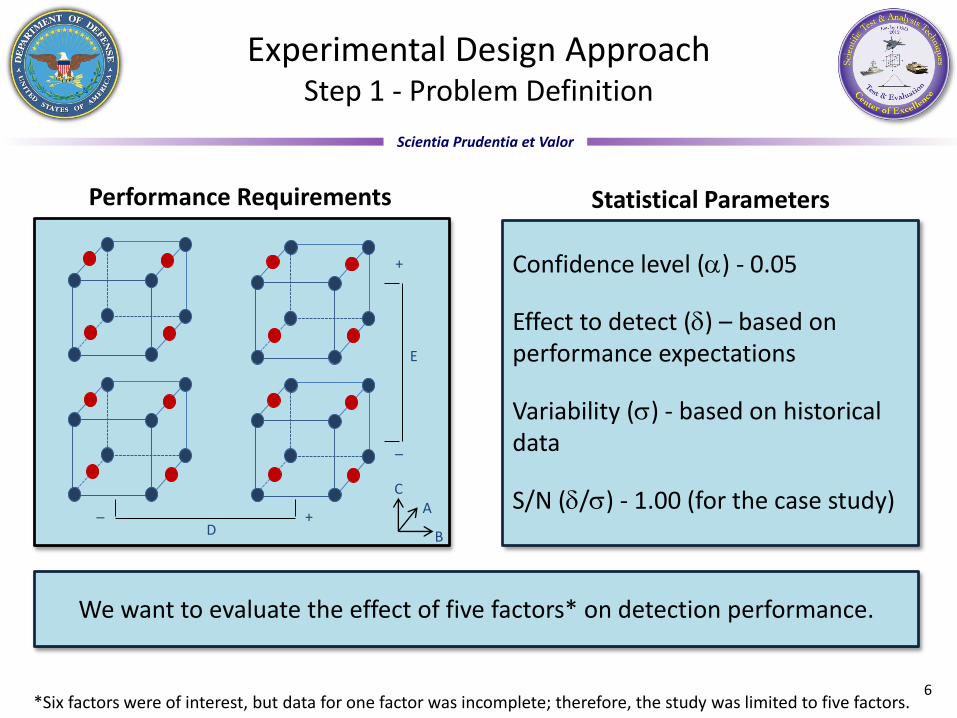
Experimental Design ApproachStep 1 - Problem Definition

Confidence level () - 0.05

Effect to detect () – based on performance expectations

Variability () - based on historical data

S/N (/) - 1.00 (for the case study)

Performance Requirements

6

D– +

E

–

+

B

AC

Statistical Parameters

We want to evaluate the effect of five factors* on detection performance.

*Six factors were of interest, but data for one factor was incomplete; therefore, the study was limited to five factors.

Scientia Prudentia et Valor

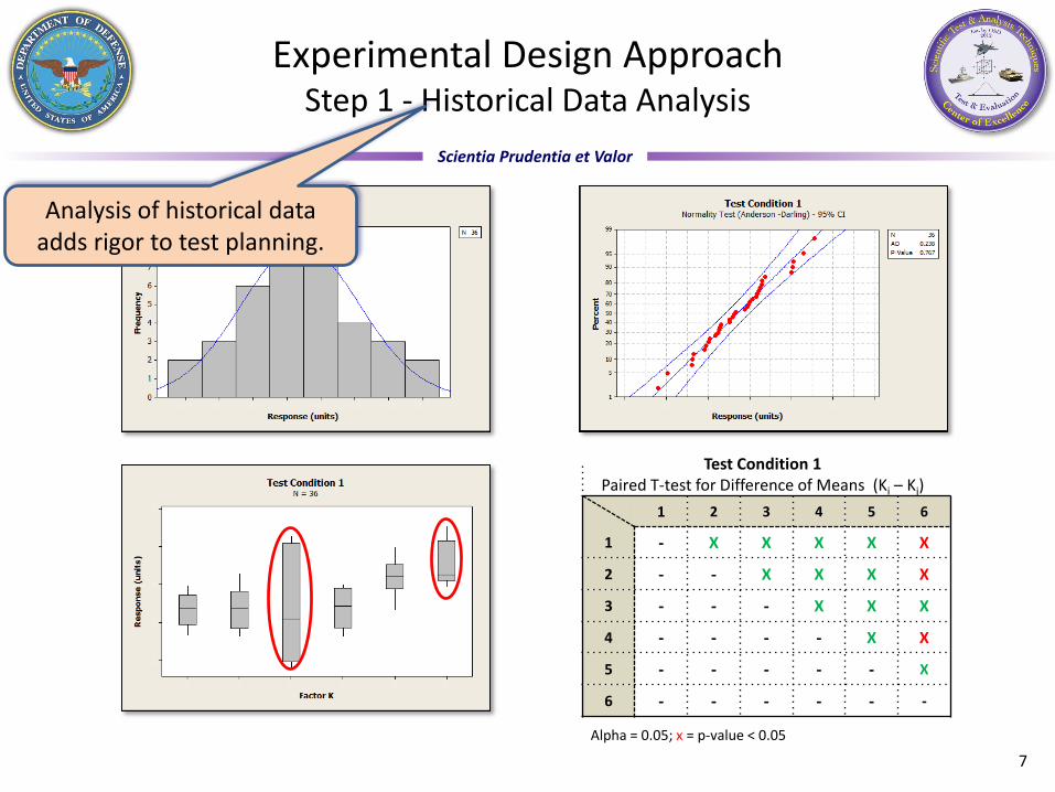
Test Condition 1Paired T-test for Difference of Means (Ki – Kj)

Alpha = 0.05; x = p-value < 0.05

1 2 3 4 5 6

1 - X X X X X

2 - - X X X X

3 - - - X X X

4 - - - - X X

5 - - - - - X

6 - - - - - -

7

Experimental Design ApproachStep 1 - Historical Data Analysis

Analysis of historical data adds rigor to test planning.

Scientia Prudentia et Valor

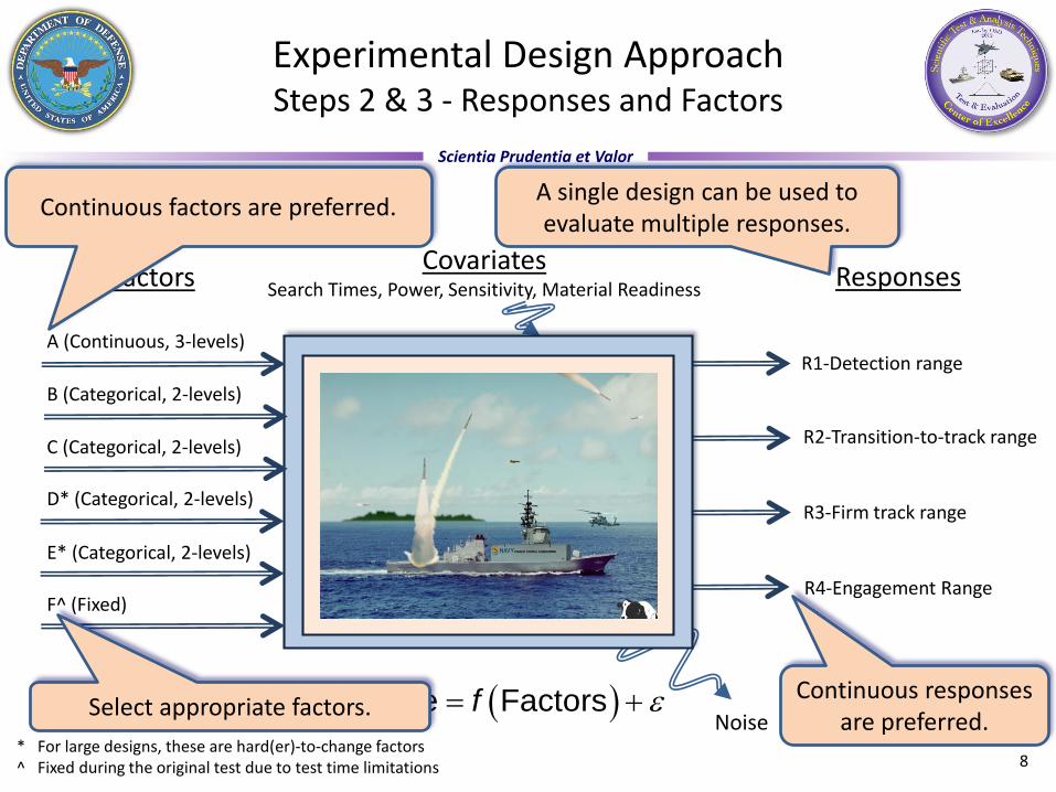
CovariatesSearch Times, Power, Sensitivity, Material Readiness

Noise

A (Continuous, 3-levels)

E* (Categorical, 2-levels)

C (Categorical, 2-levels)

B (Categorical, 2-levels)

R1-Detection range

D* (Categorical, 2-levels)

* For large designs, these are hard(er)-to-change factors^ Fixed during the original test due to test time limitations

Experimental Design ApproachSteps 2 & 3 - Responses and Factors

R2-Transition-to-track range

R3-Firm track range

R4-Engagement RangeF^ (Fixed)

8

ResponsesFactors

Response FactorsfSelect appropriate factors.

Continuous factors are preferred.A single design can be used to evaluate multiple responses.

Continuous responses are preferred.

Scientia Prudentia et Valor

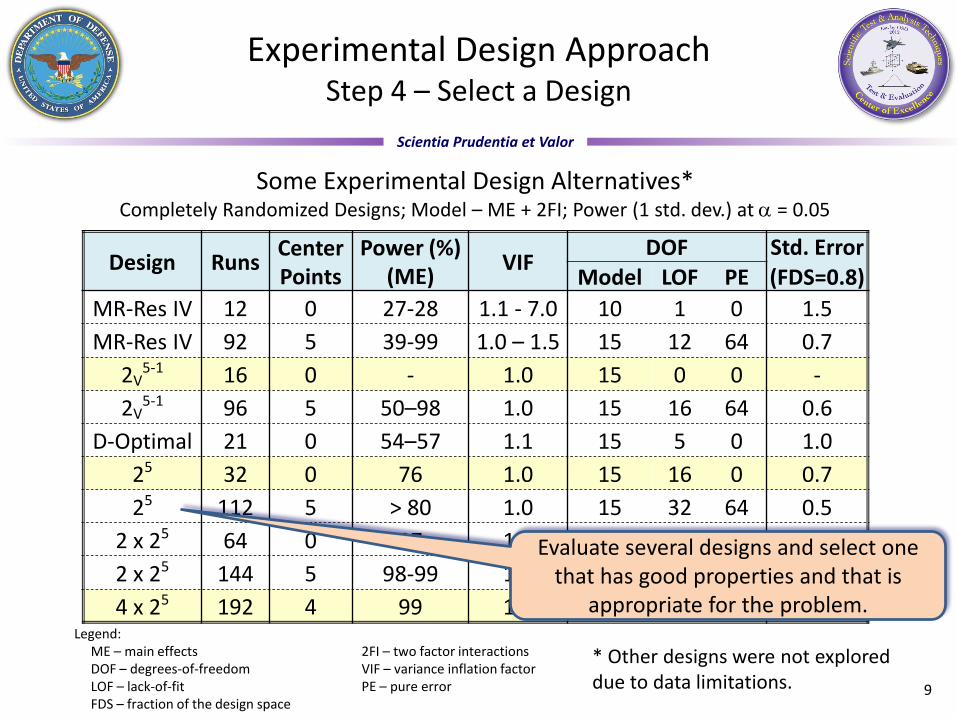
Experimental Design ApproachStep 4 – Select a Design

Design RunsCenter Points

Power (%)(ME)

VIFDOF Std. Error

Model LOF PE (FDS=0.8)

MR-Res IV 12 0 27-28 1.1 - 7.0 10 1 0 1.5

MR-Res IV 92 5 39-99 1.0 – 1.5 15 12 64 0.7

2V5-1 16 0 - 1.0 15 0 0 -

2V5-1 96 5 50–98 1.0 15 16 64 0.6

D-Optimal 21 0 54–57 1.1 15 5 0 1.0

25 32 0 76 1.0 15 16 0 0.7

25 112 5 > 80 1.0 15 32 64 0.5

2 x 25 64 0 97 1.0 15 16 32 0.5

2 x 25 144 5 98-99 1.0 15 32 96 0.4

4 x 25 192 4 99 1.0 15 32 144 0.3

Some Experimental Design Alternatives*Completely Randomized Designs; Model – ME + 2FI; Power (1 std. dev.) at = 0.05

9

Legend:ME – main effects 2FI – two factor interactionsDOF – degrees-of-freedom VIF – variance inflation factorLOF – lack-of-fit PE – pure errorFDS – fraction of the design space

Evaluate several designs and select one that has good properties and that is

appropriate for the problem.

* Other designs were not explored due to data limitations.

Scientia Prudentia et Valor

D– +

E

–

+

BA

C

Experimental Design ApproachStep 4 – Design Selection

Case I: 2V5-1 fractional factorial

16 runs

No degrees of freedom for estimating pure error, lack-of-fit, or test of significance

Case II: 25 factorial – 2 replicates 32 runs

No center points

Case III: 25 factorial + center point – 4 reps. 192 runs

Center points allow testing for curvature and estimating pure error.

10

D– +

E

–

+

BA

C

D– +

E

–

+

BA

C

Scientia Prudentia et Valor

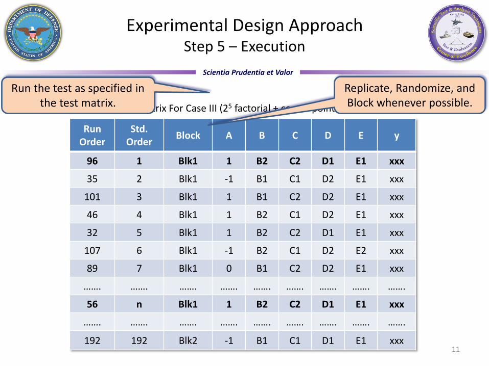
Run Order

Std. Order

Block A B C D E y

96 1 Blk1 1 B2 C2 D1 E1 xxx

35 2 Blk1 -1 B1 C1 D2 E1 xxx

101 3 Blk1 1 B1 C2 D2 E1 xxx

46 4 Blk1 1 B2 C1 D2 E1 xxx

32 5 Blk1 1 B2 C2 D1 E1 xxx

107 6 Blk1 -1 B2 C1 D2 E2 xxx

89 7 Blk1 0 B1 C2 D2 E1 xxx

……. ……. ……. ……. ……. ……. ……. ……. …….

56 n Blk1 1 B2 C2 D1 E1 xxx

……. ……. ……. ……. ……. ……. ……. ……. …….

192 192 Blk2 -1 B1 C1 D1 E1 xxx

Partial Test Matrix For Case III (25 factorial + center points; 4 replicates)

Experimental Design ApproachStep 5 – Execution

11

Run the test as specified in the test matrix.

Replicate, Randomize, and Block whenever possible.

Scientia Prudentia et Valor

Experimental Design ApproachStep 6 - Statistical Analysis (Case I)

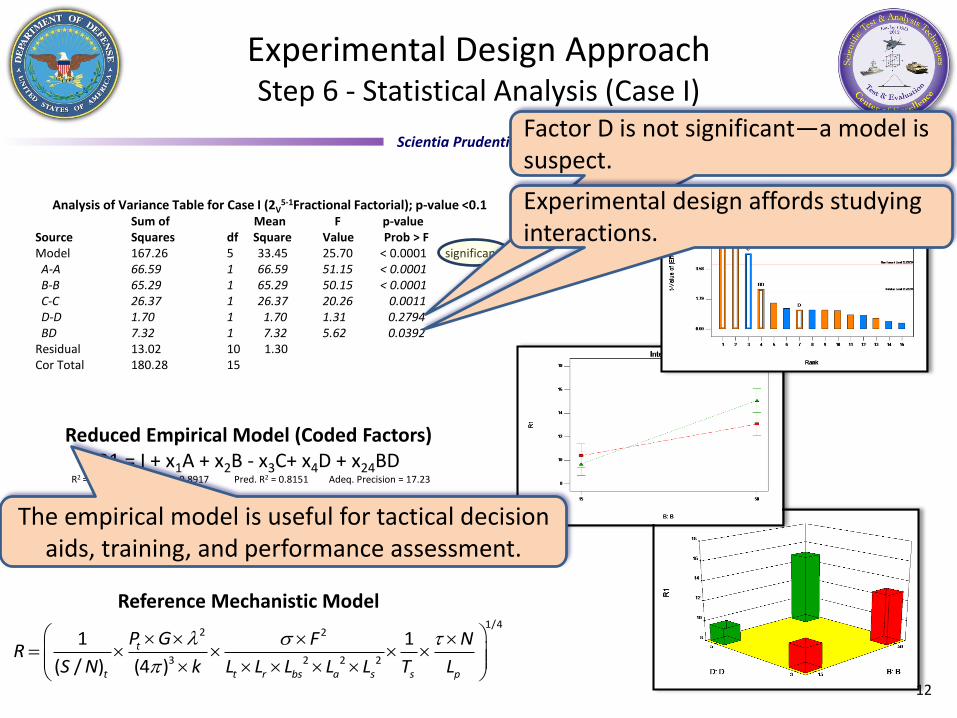
Analysis of Variance Table for Case I (2V5-1Fractional Factorial); p-value <0.1

Sum of Mean F p-valueSource Squares df Square Value Prob > FModel 167.26 5 33.45 25.70 < 0.0001 significantA-A 66.59 1 66.59 51.15 < 0.0001B-B 65.29 1 65.29 50.15 < 0.0001C-C 26.37 1 26.37 20.26 0.0011D-D 1.70 1 1.70 1.31 0.2794BD 7.32 1 7.32 5.62 0.0392

Residual 13.02 10 1.30Cor Total 180.28 15

12

Reduced Empirical Model (Coded Factors)R1 = I + x1A + x2B - x3C+ x4D + x24BD

R2 = 0.9278 Adj. R2 = 0.8917 Pred. R2 = 0.8151 Adeq. Precision = 17.23

Reference Mechanistic Model

1/42 2

3 2 2 2

1 1

( / ) (4 )t

t t r bs a s s p

P G F NR

S N k L L L L L T L

Factor D is not significant—a model is suspect.

Experimental design affords studying interactions.

The empirical model is useful for tactical decision aids, training, and performance assessment.

Scientia Prudentia et Valor

Experimental Design ApproachStep 6 - Statistical Analysis (Case I)

Only factors A, B, and C and interaction BD are significant; factor E is dropped from consideration—the sparsity of effects principle.

A Res V fractional factorial design contains a complete factorial in any subset of 4 factors—the projection property.

We can combine the runs of fractional factorials to assemble a larger design (two blocks)—sequential experimentation

13

D– +

E

–

+

BA

C

BA

CD– +

Dof for evaluation; model – ME + 2FIModel 10Residuals 5

Lack Of Fit 5Pure Error 0

Total 15

Power – 37% (1 std. dev.); 89% (2 std. dev.)

Dof for evaluation; model – ME + 2FIModel 15Residuals 0

Lack Of Fit 0Pure Error 0

Total 15

Unable to calculate power

Sparsity of effects

Projection property

Sequential experimentation

2V5-1 Fractional Factorial 24 Factorial

Scientia Prudentia et Valor

Sum of Mean F p-valueSource Squares df Square Value Prob > FModel 627.68 6 104.61 139.00 < 0.0001 significantA 216.38 1 216.38 287.51 < 0.0001B 303.20 1 303.20 402.85 < 0.0001C 94.92 1 94.92 126.11 < 0.0001E 0.27 1 0.27 0.36 0.5513BC 3.35 1 3.35 4.45 0.0393BE 9.56 1 9.56 12.71 0.0007

Residual 42.90 57 0.75Lack of Fit 19.01 25 0.76 1.02 0.4742 not significantPure Error 23.89 32 0.75Cor Total 670.58 63

Reduced Empirical Model (Coded Factors)

R = I + x1A + x2B + x3C –x4E + x23BC – x25BE

R2 = 0.9360 Adj. R2 = 0.9293 Pred. R2 = 0.9193 Adeq. Precision = 39.2

Analysis of Variance Table for Case I (2V5-1Fractional Factorial); p-value <0.1

Experimental Design ApproachStep 6 - Statistical Analysis (Case II)

14

Factor D has no significant effect on the response.

F-values consistent with complete randomization.

Continuous

Continuous factors yield response surfaces.

Scientia Prudentia et Valor

Experimental Design ApproachStep 6 – Diagnostics (Case II)

15

Design

25 Factorial2 Replicates

Validating the data and the statistical assumptions.

Scientia Prudentia et Valor

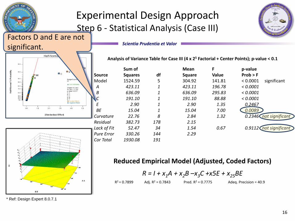
Sum of Mean F p-valueSource Squares df Square Value Prob > FModel 1524.59 5 304.92 141.81 < 0.0001 significant

A 423.11 1 423.11 196.78 < 0.0001B 636.09 1 636.09 295.83 < 0.0001C 191.10 1 191.10 88.88 < 0.0001E 2.90 1 2.90 1.35 0.2467BE 15.04 1 15.04 7.00 0.0089

Curvature 22.76 8 2.84 1.32 0.2346 not significantResidual 382.73 178 2.15Lack of Fit 52.47 34 1.54 0.67 0.9112 not significantPure Error 330.26 144 2.29Cor Total 1930.08 191

Reduced Empirical Model (Adjusted, Coded Factors)

R = I + x1A + x2B –x3C +x5E + x25BER2 = 0.7899 Adj. R2 = 0.7843 Pred. R2 = 0.7775 Adeq. Precision = 40.9

Analysis of Variance Table for Case III (4 x 25 Factorial + Center Points); p-value < 0.1

* Ref: Design Expert 8.0.7.1

16

Experimental Design ApproachStep 6 - Statistical Analysis (Case III)

Factors D and E are not significant.

Scientia Prudentia et Valor

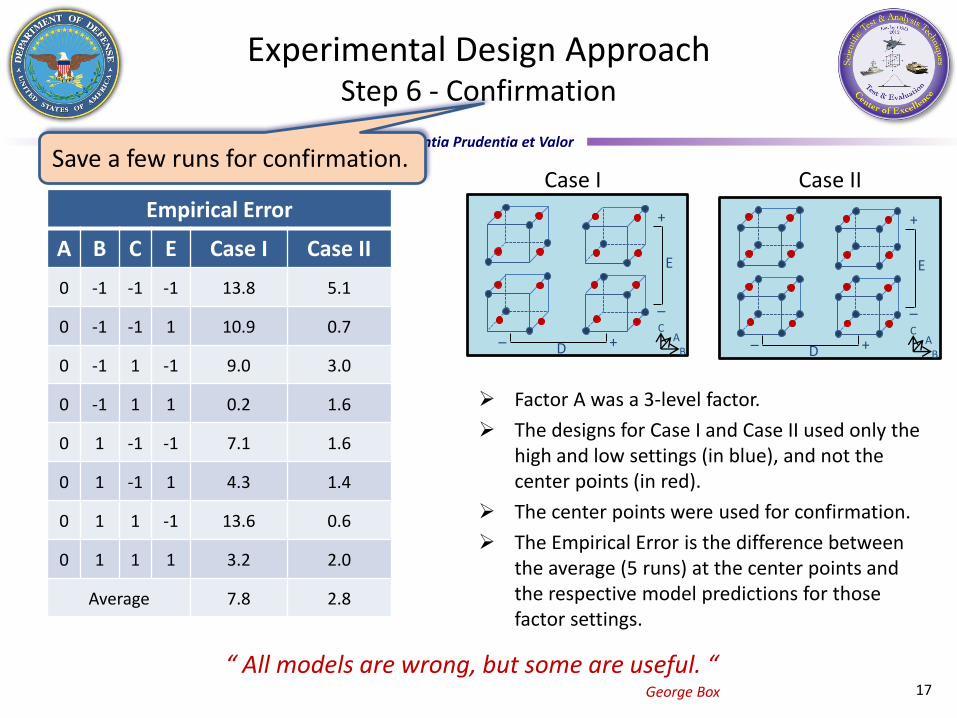
Empirical Error

A B C E Case I Case II

0 -1 -1 -1 13.8 5.1

0 -1 -1 1 10.9 0.7

0 -1 1 -1 9.0 3.0

0 -1 1 1 0.2 1.6

0 1 -1 -1 7.1 1.6

0 1 -1 1 4.3 1.4

0 1 1 -1 13.6 0.6

0 1 1 1 3.2 2.0

Average 7.8 2.8

Factor A was a 3-level factor.

The designs for Case I and Case II used only the high and low settings (in blue), and not the center points (in red).

The center points were used for confirmation.

The Empirical Error is the difference between the average (5 runs) at the center points and the respective model predictions for those factor settings.

Experimental Design ApproachStep 6 - Confirmation

17

Save a few runs for confirmation.

“ All models are wrong, but some are useful. “ George Box

D– +

E

–

+

BA

C

D– +

E

–

+

BA

C

Case I Case II

Scientia Prudentia et Valor

D = -1

E = 1

D = -1

E = -1

D = 1

E = -1

D = 1

E = 1

23

CR

D o

n A

, B

, C

23

CR

D o

n A

, B

, C

23

CR

D o

n A

, B

, C

23

CR

D o

n A

, B

, C

Test 1

23

CR

D o

n A

, B

, C

23

CR

D o

n A

, B

, C

D = -1 D = 1

Test 2

Improvements

18

Experimental Design ApproachTest 2

Screening the factors resulted in 50% reduction in runs from test to test.

Scientia Prudentia et Valor

Sum of Mean F p-valueSource Squares df Square Value Prob > FModel 350.07 7 50.01 310.41 < 0.0001 significant

A 137.99 1 137.99 856.50 < 0.0001B 187.65 1 187.65 1164.74 < 0.0001C 15.83 1 15.83 98.29 < 0.0001D 4.20 1 4.20 26.06 < 0.0001

AB 3.23 1 3.23 20.06 0.0002 AC 0.58 1 0.58 3.57 0.0710BC 0.59 1 0.59 3.67 0.0674Residual 3.87 24 0.16

Lack of fit 1.68 8 0.21 1.53 0.2231 not significantPure Error 2.19 16 0.14

Cor Total 353.93 31

Reduced Empirical Model (Coded Factors)

R = I + x1A + x2B – x3C + x4D + x12AB + x13AC – x23BCR2 = 0.9891 Adj. R2 = 0.9859 Pred. R2 = 0.9806 Adeq. Precision = 55.5

Analysis of Variance Table for Test 2 (2 x 24 Factorial); p-value < 0.1

* Ref: Design Expert 8.0.7.1

19

Experimental Design ApproachStep 6 - Statistical Analysis (Test 2, Case II)

Factors D now is significant.

Scientia Prudentia et Valor

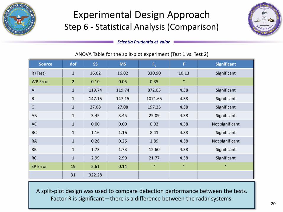
Source dof SS MS F0 F Significant

R (Test) 1 16.02 16.02 330.90 10.13 Significant

WP Error 2 0.10 0.05 0.35 *

A 1 119.74 119.74 872.03 4.38 Significant

B 1 147.15 147.15 1071.65 4.38 Significant

C 1 27.08 27.08 197.25 4.38 Significant

AB 1 3.45 3.45 25.09 4.38 Significant

AC 1 0.00 0.00 0.03 4.38 Not significant

BC 1 1.16 1.16 8.41 4.38 Significant

RA 1 0.26 0.26 1.89 4.38 Not significant

RB 1 1.73 1.73 12.60 4.38 Significant

RC 1 2.99 2.99 21.77 4.38 Significant

SP Error 19 2.61 0.14 * * *

31 322.28

20

Experimental Design ApproachStep 6 - Statistical Analysis (Comparison)

ANOVA Table for the split-plot experiment (Test 1 vs. Test 2)

A split-plot design was used to compare detection performance between the tests. Factor R is significant—there is a difference between the radar systems.

Scientia Prudentia et Valor

Experimental design is the integration of well defined and structured scientific strategies for gathering empirical knowledge using statistical methods for planning, designing, executing, and analyzing a test.

Experimental design provides a comprehensive understanding of the trade-offs in the techno-programmatic domains: risks, cost, and utility of information.

Experimental design can help reducing test assets, shortening the test schedule, and providing more information to the warfighter and decision makers.

Experimental design adds rigor and discipline to T&E.

Summary

21

Scientia Prudentia et Valor

Conclusions

What could we have done differently?

Only 16 runs

+ center points

+ axial points

(maybe)22

Scientia Prudentia et Valor

References

Bisgaard, S., Fuller, H. T., & Barrios, E. (1996). Quality quandaries: Two-level factorials run as split-plot experiments. Quality Engineering, 8, 705-708

Coleman, D. D., & Montgomery, D. C. (1993). A systematic approach to planning for a designed industrial experiment. Technometrics, 35, 1-12.

Cortes, L. A., & Bergstrom, D. (2012). Using design of experiments for the assessment of surface radar detection performance and compliance with critical technical parameters. 80th MORS Symposium, June 2012.

Fisher, R. A. (1962). The place of the design of experiments in the logic of scientific inference. Colloques Internationaux du Centre National de la Recherche Scientifique,110, 13-19.

Freeman, L. J., Ryan, A. G., Kensler, J. L. K., Dickinson, R. M., & Vining, G. G. (2013). A tutorial on the planning of experiments. Quality Engineering, 25, 315-332.

Johnson, R. T., Hutto, G. T., Simpson, J. R., & Montgomery, D. C. (2012). Designed experiments for the defense community, Quality Engineering, 24, 60-79.

Montgomery, D. C. (2013), Design and Analysis of Experiments,8th ed., John Wiley & Sons.

Simpson, J. R., Listak, C. M., & Hutto, G. T. (2013). Guidelines for planning and evidence for assessing a well-designed experiment. Quality Engineering, 25, 316-355. 23

Knowledge, insight, and value24