Radial Basis Functions and Vortex Methods and their - Deep Blue

Radial Basis Functions and Vortex Methods and

their Application to Vortex Dynamics on a

Rotating Sphere

by

Lei Wang

A dissertation submitted in partial fulfillmentof the requirements for the degree of

Doctor of Philosophy(Applied and Interdisciplinary Mathematics)

in The University of Michigan2010

Doctoral Committee:

Professor John P. Boyd, Co-ChairProfessor Robert Krasny, Co-ChairAssociate Professor Divakar ViswanathAssistant Professor Christiane Jablonowski

c© Lei Wang 2010All Rights Reserved

To the memory of Meiyu Zheng. I miss you and think of you often.

ii

ACKNOWLEDGEMENTS

This thesis work could not have been finished without the help from a number of

persons to whom I owe a great debt of gratitude, and I would like to thank them for

their valuable contributions.

First, I want to express my deep and sincere appreciation to Professor Robert

Krasny, who supervised my study and research work during the past five years.

The high standard he always sets for himself has been inspiring to me. Besides the

knowledge he has given me, I am particularly grateful for his enormous patience and

encouragement during several difficult times.

I would also like to sincerely thank to Professor John P. Boyd as my advisor

outside the math department, who also supervised my studies and research during

the past five years. Professor Boyd’s wide knowledge and logical way of thinking

have been of great value to me. He is the person who taught me to do math in a

different way.

I want to express my gratitude to Professor Christiane Jablonowski, Professor

Divakar Viswanath and Professor Smadar Karni. Their help and support have been

invaluable.

Last but not least, I want to thank my husband, Danqing Wu, and my other

family members in China, for the love and support they have provided.

iii

TABLE OF CONTENTS

DEDICATION . . . . . . . . . . . . . . . . . . . . . . . . . . . . . . . . . . . . . . . . . . ii

ACKNOWLEDGEMENTS . . . . . . . . . . . . . . . . . . . . . . . . . . . . . . . . . . iii

LIST OF FIGURES . . . . . . . . . . . . . . . . . . . . . . . . . . . . . . . . . . . . . . vii

LIST OF TABLES . . . . . . . . . . . . . . . . . . . . . . . . . . . . . . . . . . . . . . . xii

CHAPTER

I. Introduction . . . . . . . . . . . . . . . . . . . . . . . . . . . . . . . . . . . . . . . 1

1.1 Motivation for Thesis . . . . . . . . . . . . . . . . . . . . . . . . . . . . . . . 11.2 Overview of Thesis Topics . . . . . . . . . . . . . . . . . . . . . . . . . . . . 5

II. Radial Basis Function Analysis . . . . . . . . . . . . . . . . . . . . . . . . . . . 7

2.1 Introduction . . . . . . . . . . . . . . . . . . . . . . . . . . . . . . . . . . . . 72.2 RBFs Accuracy and Stability . . . . . . . . . . . . . . . . . . . . . . . . . . 92.3 Computational cost . . . . . . . . . . . . . . . . . . . . . . . . . . . . . . . . 112.4 Basic Formulas for Gaussian RBF . . . . . . . . . . . . . . . . . . . . . . . . 13

2.4.1 Computing the coefficients of an RBF expansion . . . . . . . . . . 142.4.2 Poisson summation . . . . . . . . . . . . . . . . . . . . . . . . . . . 15

2.5 Cardinal Function . . . . . . . . . . . . . . . . . . . . . . . . . . . . . . . . . 152.5.1 Derivation . . . . . . . . . . . . . . . . . . . . . . . . . . . . . . . . 16

2.6 Comparison to Finite Differences Using Fourier Analysis . . . . . . . . . . . 192.6.1 Eigenvalues of the RBF difference operators for exp(iKX) . . . . . 192.6.2 Numerical experiments . . . . . . . . . . . . . . . . . . . . . . . . . 21

III. Fast Treecode for Evaluating RBFs . . . . . . . . . . . . . . . . . . . . . . . . . 25

3.1 Introduction . . . . . . . . . . . . . . . . . . . . . . . . . . . . . . . . . . . . 253.2 Build Tree . . . . . . . . . . . . . . . . . . . . . . . . . . . . . . . . . . . . . 263.3 Particle-Cluster Interaction . . . . . . . . . . . . . . . . . . . . . . . . . . . . 28

3.3.1 Well-separated particle-cluster interaction list 1 . . . . . . . . . . . 293.3.2 Well-separated particle-cluster interaction list 2 . . . . . . . . . . . 293.3.3 Far field expansion . . . . . . . . . . . . . . . . . . . . . . . . . . . 31

3.4 Recurrence Relation for Taylor Series . . . . . . . . . . . . . . . . . . . . . . 323.4.1 Multiquadric . . . . . . . . . . . . . . . . . . . . . . . . . . . . . . 323.4.2 Gaussian . . . . . . . . . . . . . . . . . . . . . . . . . . . . . . . . . 333.4.3 Inverse multiquadric . . . . . . . . . . . . . . . . . . . . . . . . . . 34

3.5 Treecode Algorithm . . . . . . . . . . . . . . . . . . . . . . . . . . . . . . . . 343.6 Cartesian Taylor Treecode for Multiquadric RBF . . . . . . . . . . . . . . . 35

3.6.1 Far field expansion for multiquadric in 1D . . . . . . . . . . . . . . 36

iv

3.6.2 The generalized multiquadric in muti-D . . . . . . . . . . . . . . . 383.6.3 Treecode performance . . . . . . . . . . . . . . . . . . . . . . . . . 403.6.4 Random nodes in a cube . . . . . . . . . . . . . . . . . . . . . . . . 423.6.5 Random nodes on a sphere . . . . . . . . . . . . . . . . . . . . . . 44

IV. Barotropic Vorticity Equation . . . . . . . . . . . . . . . . . . . . . . . . . . . . 48

4.1 Introduction . . . . . . . . . . . . . . . . . . . . . . . . . . . . . . . . . . . . 484.2 Solution of Poisson Equation on the Sphere . . . . . . . . . . . . . . . . . . . 50

4.2.1 Spherical harmonics . . . . . . . . . . . . . . . . . . . . . . . . . . 504.2.2 Green’s function . . . . . . . . . . . . . . . . . . . . . . . . . . . . 524.2.3 Regularized Green’s Function . . . . . . . . . . . . . . . . . . . . . 564.2.4 Gaussian forcing . . . . . . . . . . . . . . . . . . . . . . . . . . . . 57

4.3 Rossby-Haurwitz Wave . . . . . . . . . . . . . . . . . . . . . . . . . . . . . . 594.3.1 Stream function . . . . . . . . . . . . . . . . . . . . . . . . . . . . . 594.3.2 Example . . . . . . . . . . . . . . . . . . . . . . . . . . . . . . . . . 60

V. Solving the Barotropic Vorticity Equation by Gaussian RBF . . . . . . . . 64

5.1 Soving PDEs by RBF . . . . . . . . . . . . . . . . . . . . . . . . . . . . . . . 645.2 Solving BVE by Gaussian RBF . . . . . . . . . . . . . . . . . . . . . . . . . 655.3 Rossby-Haurwitz Wave . . . . . . . . . . . . . . . . . . . . . . . . . . . . . . 685.4 One Vortex Patch . . . . . . . . . . . . . . . . . . . . . . . . . . . . . . . . . 71

5.4.1 Choosing RBF parameter ε . . . . . . . . . . . . . . . . . . . . . . 715.5 Two Vortex Patches on a Non-rotating Sphere . . . . . . . . . . . . . . . . . 74

5.5.1 Initial patches . . . . . . . . . . . . . . . . . . . . . . . . . . . . . . 755.5.2 Numerical integration . . . . . . . . . . . . . . . . . . . . . . . . . 76

VI. Solving the Barotropic Vorticity Equation by Vortex Method . . . . . . . . 78

6.1 Introduction . . . . . . . . . . . . . . . . . . . . . . . . . . . . . . . . . . . . 786.2 Lagrangian Fomulation of BVE . . . . . . . . . . . . . . . . . . . . . . . . . 796.3 Meshes on the Surface of the Sphere . . . . . . . . . . . . . . . . . . . . . . . 81

6.3.1 Longitude-latitude (LL) . . . . . . . . . . . . . . . . . . . . . . . . 816.3.2 Icosahedral triangles (IT) . . . . . . . . . . . . . . . . . . . . . . . 826.3.3 Icosahedral hexagon (IH) . . . . . . . . . . . . . . . . . . . . . . . 836.3.4 Cubed-sphere (CS) . . . . . . . . . . . . . . . . . . . . . . . . . . . 84

6.4 Area for Panels on Sphere . . . . . . . . . . . . . . . . . . . . . . . . . . . . 876.5 Regularized Approximation . . . . . . . . . . . . . . . . . . . . . . . . . . . . 886.6 Rossby-Haurwitz Wave Experiments . . . . . . . . . . . . . . . . . . . . . . . 89

6.6.1 Definition of error . . . . . . . . . . . . . . . . . . . . . . . . . . . . 906.6.2 Mesh comparison . . . . . . . . . . . . . . . . . . . . . . . . . . . . 906.6.3 Timestep experiments . . . . . . . . . . . . . . . . . . . . . . . . . 906.6.4 Test spatial error . . . . . . . . . . . . . . . . . . . . . . . . . . . . 916.6.5 Stream function . . . . . . . . . . . . . . . . . . . . . . . . . . . . . 916.6.6 Nonuniform mesh test . . . . . . . . . . . . . . . . . . . . . . . . . 92

6.7 Adaptive Mesh Refinement (AMR) . . . . . . . . . . . . . . . . . . . . . . . 946.8 Gaussian Vortex Tests . . . . . . . . . . . . . . . . . . . . . . . . . . . . . . . 96

6.8.1 Non-rotating sphere . . . . . . . . . . . . . . . . . . . . . . . . . . 976.8.2 Rotating sphere . . . . . . . . . . . . . . . . . . . . . . . . . . . . . 986.8.3 Convergence check . . . . . . . . . . . . . . . . . . . . . . . . . . . 98

6.9 Two Gaussian Vortices Test . . . . . . . . . . . . . . . . . . . . . . . . . . . 996.9.1 Non-rotating sphere . . . . . . . . . . . . . . . . . . . . . . . . . . 1026.9.2 Rotating sphere . . . . . . . . . . . . . . . . . . . . . . . . . . . . . 102

v

6.10 Remeshing . . . . . . . . . . . . . . . . . . . . . . . . . . . . . . . . . . . . . 1046.11 Comparison of Vortex Method with GARBF Method . . . . . . . . . . . . . 104

VII. Summary and Future work . . . . . . . . . . . . . . . . . . . . . . . . . . . . . . 107

7.1 Thesis Summary . . . . . . . . . . . . . . . . . . . . . . . . . . . . . . . . . . 1077.2 Improving the Vortex/RBF Method for solving BVE . . . . . . . . . . . . . 1087.3 Shallow Water Equation (SWE) . . . . . . . . . . . . . . . . . . . . . . . . . 1097.4 Application and Extension of Treecode . . . . . . . . . . . . . . . . . . . . . 1097.5 Jet Simulation . . . . . . . . . . . . . . . . . . . . . . . . . . . . . . . . . . . 110

BIBLIOGRAPHY . . . . . . . . . . . . . . . . . . . . . . . . . . . . . . . . . . . . . . . . 111

vi

LIST OF FIGURES

Figure

1.1 Hierarchy of climate models (from John Thuburn, University of Exeter). . . . . . . 2

1.2 A sphere rotates around the z-axis with angular velocity Ω. . . . . . . . . . . . . . 3

2.1 Gaussian RBF and MQ RBF for different shape parameter ε. The figures showthat the basis function become flatter as ε→ 0. . . . . . . . . . . . . . . . . . . . . 10

2.2 Gaussian RBF approximation of the Runge function (2.8) on a uniform grid withN = 41 for different ε. ((a)-(d)): f (red line) and interpolation function s(x) (blue) versus x; ((e)-(h)): error versus x. Errors are decreasing first then increasingwhen ε changes from 20 to 0.5. . . . . . . . . . . . . . . . . . . . . . . . . . . . . . 12

2.3 Cardinal function in equation (2.25) for different α. It equals one when X = 0 andzero for the other integers. . . . . . . . . . . . . . . . . . . . . . . . . . . . . . . . . 17

2.4 The shaded regions show where the absolute error in the eigenvalue of the firstderivative, K − κ(K;M), is smaller than 0.05 for four different values of M as afunction of α. . . . . . . . . . . . . . . . . . . . . . . . . . . . . . . . . . . . . . . . 22

2.5 Finite difference error divided by Gaussian RBF error in the eigenvalue of the firstderivative versus K for M = 4, 8, 16, which is a stencil of nine, seventeen and thirtythree points with different α. The thick dashed horizontal line is where the ratiois one: the radial basis function method is better whenever the ratio is above thisline, and the finite difference is better whenever the curve is below this dashed line.The thin dotted line marks the right one-third of the spectrum which would beremoved by a dealiasing filter in a hydrodynamics computation. . . . . . . . . . . . 23

3.1 Complete hierarchical tree structure in two dimension for 4 levels. Level = 0 is alsocalled the root cluster. . . . . . . . . . . . . . . . . . . . . . . . . . . . . . . . . . . 27

3.2 Adaptive hierarchical tree structure in two dimensions for N0 = 1, where N0 is themaximum number of particles in a leaf. . . . . . . . . . . . . . . . . . . . . . . . . . 28

3.3 Example of neighbors and well separated panels for a complete tree. The targetpoints are in the red cell, the white cells are the neighbors and the blue cells arethe well separated cells of the red cell. . . . . . . . . . . . . . . . . . . . . . . . . . 30

3.4 Particle cluster interaction when r/R < θ, where r is the radius of the cluster andθ is MAC number. (a): Barnes and Hut [7]; R is the distance between x and thecenter of the cluster yC ; (b): Barnes [6], R is the distance between the centers ofthe two clusters. . . . . . . . . . . . . . . . . . . . . . . . . . . . . . . . . . . . . . 31

vii

3.5 Example of 2d stencils for recurrence relation. Taylor coefficients at blue point onlydepends on the coefficients at four red points. . . . . . . . . . . . . . . . . . . . . . 34

3.6 Flowchart of Barnes and Hut [7] treecode algorithm. (a) main function and (b)subroutine compute interaction. Note that there is a recursive call in the subroutine. 35

3.7 Schematic showing branch points, branch cuts, and domain of convergence (shaded)for far-field expansions of φ(x) given in (3.16); (a) the Laurent series (3.17) con-verges outside a disk in the x-plane; (b) the Taylor series (3.19) converges inside adisk in the y-plane. As c increases, the shaded region in (a) becomes smaller andthe shaded region in (b) becomes larger. . . . . . . . . . . . . . . . . . . . . . . . 36

3.8 Example in 1D from [10] showing a cluster C of nodes satisfying |yj | ≤ h andwell-separated evaluation points satisfying |xi| ≥ 3h. . . . . . . . . . . . . . . . . . 38

3.9 A well separated particle-cluster interaction example for testing the convergence ofLaurent expansion (3.24) and Taylor expansion (3.26). . . . . . . . . . . . . . . . . 41

3.10 Error (3.36) in a particle-cluster approximation with one evaluation point at theorigin in R3 and a cluster of N = 103 random nodes in the cube [0.75, 1]3; ν =1, d = 3. The error is plotted as a function of the RBF parameter c and order p, for10−3 ≤ c ≤ 103 and p = 0 : 2 : 10. (a) Laurent series (3.24), (b) Taylor series (3.29). 41

3.11 N random points in a cube (left) and on the surface of a sphere. . . . . . . . . . . 42

3.12 Random nodes in a cube, scatter plot of CPU time and error (3.37), data fromTable 3.1, system size N = 216K, order p = 0 : 2 : 10 (increasing from right toleft), MAC parameter θ = 0.2 (,black), θ = 0.5 (∗,red), θ = 0.8 (4,blue), RBFparameter c = 10−1, maximum leaf size N0 = 200. The lower envelope of the datagives the most efficient choice of parameters (p, θ) to attain a given error. . . . . . 44

3.13 Random nodes in a cube, treecode error (3.37) plotted as a function of systemsize N = 103, 203, . . . , 1003, order p = 0 : 2 : 10, MAC parameter θ = 0.8, RBFparameter c = 10−1, maximum leaf size N0 = 200 except N0 = 400 for N = 903, 1003. 45

3.14 Random nodes in a cube, treecode CPU time in seconds, same parameters as inFigure 3.13 caption, ds denotes direct sum. . . . . . . . . . . . . . . . . . . . . . . 45

3.15 Random nodes in a cube, treecode memory usage in MB, same parameters as inFigure 3.13 caption, ds denotes direct sum. . . . . . . . . . . . . . . . . . . . . . . 46

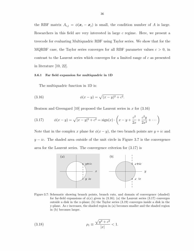
4.1 Diagram for showing the central angle between two points (θ, λ) and (θ′, λ′) onsphere. . . . . . . . . . . . . . . . . . . . . . . . . . . . . . . . . . . . . . . . . . . . 52

4.2 (a) and (b) are the plot of the vorticity ζδ (4.46) from smooth Green’s function Gδ(4.42) for δ = 0.2, 0.1, 0.05, where (b) is in log scale. Both figures share the samelegend. Note that ζδ is an approximate delta function. . . . . . . . . . . . . . . . . 57

4.3 The vorticity function ζε (4.51) with Gaussian forcing at north pole for different ε. 58

4.4 Initial stream function with amplitude A = 0.05 and n = 1,m = 1. . . . . . . . . . 60

4.5 Stream function from equation (4.63) at t = π, 2π, 3π, 4π with amplitude A = 0.05and angular velocity Ω = 1/2. . . . . . . . . . . . . . . . . . . . . . . . . . . . . . . 62

viii

4.6 Rossby-Haurwitz wave (n = m = 1). (a) : particle trajectories obtained by solvingequations (4.72) to (4.74) using fourth order Runge-Kutta for five revolutions, whereA = 0.05 and Ω = 1/2; (b): local zoom of the left figure. . . . . . . . . . . . . . . . 63

5.1 Illustration of icosahedral points on the surface of the sphere with (a) n = 20 and(b) n = 80. . . . . . . . . . . . . . . . . . . . . . . . . . . . . . . . . . . . . . . . . 69

5.2 Absolute error of vorticity defined by (5.18) which is obtained by GARBF after onerevolution (t = 4π) with N = 20, ∆t = 4π/200, ε = 0.1. . . . . . . . . . . . . . . . 70

5.3 Relative error defined by (5.19) of vorticity obtained by GARBF after one revolution(t = 4π) for the number of timesteps is 25, 50, 100, 200, 400. Total number of pointsis 20 and ε = 0.1. . . . . . . . . . . . . . . . . . . . . . . . . . . . . . . . . . . . . . 70

5.4 (a): The relative error defined by (5.19) of vorticity obtained by GARBF with∆t = 4π/200, n = 80 for different ε; (b): the condition number of RBF matrix A. . 71

5.5 Interpolation points for initial vorticity; refined spherical triangular mesh (whichwill be discussed in detail in Chapter Six); number of points is 170, minimumdistance between two points are 0.0451. . . . . . . . . . . . . . . . . . . . . . . . . 73

5.6 Absolute error of relative vorticity computed in grid in Figure 5.5. (a): fixed ε;(b): ε adoptive from (5.25). Note that the maximum error occurs where the meshchanges from coarse to fine. . . . . . . . . . . . . . . . . . . . . . . . . . . . . . . . 74

5.7 Absolute error of relative vorticity for different εmin. Note that the maximum erroroccurs where the mesh changes from coarse to fine. . . . . . . . . . . . . . . . . . 75

5.8 Points in a disk on a plane. The nNIHS = 2,4,8,16. Every point is at the center ofa hexagon. . . . . . . . . . . . . . . . . . . . . . . . . . . . . . . . . . . . . . . . . . 76

5.9 Vortex patches evolution. the ratio of the distance between two center of the patchesthe radius of the patch is 2.6. The total number of the particles is 2918. (a): twovortex patches at t = 0; (b): t = 2; (c): t = 3; (d): close up look at t = 3. . . . . . 77

6.1 Active points (•) and passive points () of a triangle and quadrilateral panel. . . . 81

6.2 Longitude-Latitude Panel. (a): side view; (b): view from north pole. Points areclustered at the pole area. . . . . . . . . . . . . . . . . . . . . . . . . . . . . . . . . 81

6.3 Icosahedral triangle mesh refinement stencils. For example, new vertices v12 is thecenter of the edge v1v2. The coordinate of the new center c1 is the average of threevertices v1, v12, v31 by equation (6.11) then project to the sphere by equation (6.12). 83

6.4 Icosahedral triangles. From left to right: L = 0, 1, 2, 3 and n = 20, 80, 320, 1280.Vertices are projections from 12 vertices of an icosahedron to a unit sphere. . . . . 83

6.5 Icosahedral triangles with local refinement. The red and yellow colors indicate somelocal features that we want to resolve and where local mesh refinement is needed. . 83

6.6 The ratio of minimum area and maximum area in Icosahedral triangle mesh. Thisshows the mesh becomes more uniform as the number of points increases. . . . . . 84

ix

6.7 Icosahedral hexagon. From left to right: L = 0, 1, 2, 3 and n = 12, 42, 162, 642. Thevertices of the hexagon/pendagon are the centers of the spherical triangle in figure(6.4). . . . . . . . . . . . . . . . . . . . . . . . . . . . . . . . . . . . . . . . . . . . . 84

6.8 a circumscribed cube in a sphere . . . . . . . . . . . . . . . . . . . . . . . . . . . . 85

6.9 Cubed-sphere mesh refinement stencils. For example, new vertices v12 is the centerof the edge v1v2. The coordinate of the new center c1 is the average of four verticesv1, v12, vc, v41 by equation (6.11) then project to the sphere by equation (6.12),where vc is at the same position as the center c. . . . . . . . . . . . . . . . . . . . . 86

6.10 Cubed-sphere mesh with n = 6, 24, 96, 384. The first eight vertices of quadrilateralpanels are the vertices of a circumscribed cube. . . . . . . . . . . . . . . . . . . . . 86

6.11 Cubed-sphere local refinement. The red and yellow colors indicate some local fea-tures that we want to resolve and where local mesh refinement is needed. . . . . . 86

6.12 Angles of the spherical triangles. . . . . . . . . . . . . . . . . . . . . . . . . . . . . 88

6.13 Absolute error in particle positions after one revolution for different meshes: icosa-hedral triangle, icosahedral hexagon and cubed-sphere for RH wave. The error iscomparable for the three meshes. All three lines are parallel to the line O(1/n),which means the vortex method we use here is first order accurate in terms of thenumber of points. . . . . . . . . . . . . . . . . . . . . . . . . . . . . . . . . . . . . . 91

6.14 Plot |AbsErr − SaturationError| versus dt, which shows the 4th order accuracy ofRK4 with N = 320, 1280. star: N = 320 ; circle: N = 1280 . . . . . . . . . . . . . . 94

6.15 RH wave: Absolute error for particle position after one revolution in sphericaltriangular mesh for ∆t = 4π/1600. n is the number of the panels on sphere. . . . 95

6.16 Trajectory of particles after five revolutions with N = 80, dt = 4π/1600, which isagree to the one we obtained from exact ODE equations (4.72) to (4.74) and figure(4.6). . . . . . . . . . . . . . . . . . . . . . . . . . . . . . . . . . . . . . . . . . . . . 96

6.17 Relative error (6.23) of the stream function (6.1) using midpoint numerical integralbased on spherical triangle (ST). Area means the maximum area of the sphericaltriangle since they are not exactly the same.) . . . . . . . . . . . . . . . . . . . . . 97

6.18 Exact and approximate (6.20) stream function for RH wave at t = 0, t = 2π, t =3π, t = 4π with n = 80 and δ = 0.02 . . . . . . . . . . . . . . . . . . . . . . . . . . 98

6.19 Meshes for N = 120, 180, 456, 1572 for testing the effect of mesh non-uniformity. . . 99

6.20 (a): absolute error for particle positions for uniform cubed-sphere mesh as in figure(6.10) and nonuniform cubed-sphere meshes as in figure (6.19); Right : ratio of twoabsolute errors defined in (6.25). . . . . . . . . . . . . . . . . . . . . . . . . . . . . 99

6.21 Gaussian patch test case 1 at t = 0, 2π, 4π on a nonrotating sphere using (a)cubed-sphere mesh and (b) icosahedral triangle mesh. The patch is self-rotatingand preserves the symmetric shape. . . . . . . . . . . . . . . . . . . . . . . . . . . 100

x

6.22 Gaussian patch test case 2 at t = 0, 2π, 4π on a rotating sphere. (a): cubed-sphere mesh; (b) icosahedral triangle mesh. Gaussian patch moves in the northwestdirection which agrees with the physical expectation. . . . . . . . . . . . . . . . . . 101

6.23 Gaussian patch test case 3. From left to right, εΓ = 0.001, 0.0005, 0.0002, 0.0001 att = 4π. We can observe qualitative convergence property. . . . . . . . . . . . . . . 101

6.24 Gaussian patch test case 4 at t = 0, π, 3π on a nonrotating sphere. The initialcenters of two patches are (−0.3670, 0.8548, 0.3670) and (0.3670, 0.8548, 0.3670).The two patches rotate around each other and merge. . . . . . . . . . . . . . . . . 103

6.25 Gaussian patch test case 5 at t = 0, π, 3π on a rotating sphere. The initial cen-ters of two patches are (−0.3670, 0.8548, 0.3670) and (0.3670, 0.8548, 0.3670). Thetwo patches rotate around each other and merge and both are drift towards thenorthwest direction. . . . . . . . . . . . . . . . . . . . . . . . . . . . . . . . . . . . 103

6.26 Preliminary results of remeshing. Retain the relative vorticity at L = 4 uniformmesh with δ = 0.02 using equation (6.22) then refined with εΓ = 0.0004 andεd = 0.02. (a) and (c) are the Gaussian patch test at t = 2π and t = 4π withΩ = 0, L = 4, εΓ = 0.0004 and εd = 0.02,∆t = 4π/1000, δ = 0.02; (b) and (d) arethe meshs after remeshing for (a) and (c) respectively. . . . . . . . . . . . . . . . . 105

7.1 Stencils for high order refinement. (a): one active point and eight passive points inquadrilateral panel; (b): one active point and 6 passive points in triangular panel. 109

7.2 Vortex sheet evolution t = 0, 15, 20 and the last one is a close-up at t = 20. . . . . . 110

xi

LIST OF TABLES

Table

2.1 Some common types of radial functions φ(r) for RBF. There are two types of radialfunctions, the piecewise smooth and the infinitely smooth radial functions. All theinfinitely smooth radial functions have a shape parameter ε. . . . . . . . . . . . . . 10

2.2 Condition number of the matrix A when interpolating Runge function using Gaus-sian RBF on a uniform grid with N = 41. . . . . . . . . . . . . . . . . . . . . . . . 13

3.1 Random nodes in a cube, the treecode error (3.37) and CPU time (sec) are givenfor system size N = 216K, RBF parameter c = 10−1, order p = 0 : 2 : 10, MACparameter θ = 0.2, 0.5, 0.8, maximum leaf size N0 = 200. . . . . . . . . . . . . . . . 43

3.2 Random nodes in a cube and on a sphere, tc denotes treecode and ds denotesdirect sum, CPU time in seconds and memory in MB, RBF parameter c = 10−1,maximum leaf size N0 = 200 except N0 = 400 for N = 1000K, order p = 6, MACparameter θ = 0.8. . . . . . . . . . . . . . . . . . . . . . . . . . . . . . . . . . . . . 47

5.1 Relative Error for RBF approximation on a sphere with fixed number of interpola-tion points and different ε (uniform). α is defined in equation (5.24). . . . . . . . 73

5.2 Condition number for εmin = 1, 0.8, 0.6, 0.4. . . . . . . . . . . . . . . . . . . . . . . 74

6.1 Absolute Error for particle positions after one revolution, N = 320. The errorsaturates around 0.004339 due to the spatial discretization. . . . . . . . . . . . . . 92

6.2 Absolute error for particle positions after one revolution, N = 1280. The errorsaturate around 0.001244 due to the spacial discretization. . . . . . . . . . . . . . . 93

6.3 Absolute error for particle position after one revolution with fixed ∆t = 0.00785 inicosahedral triangular mesh for different spacial resolution N = 20, 80, 320, 1280. . . 93

6.4 Parameters for Gaussian patch tests. CS = cubed-sphere mesh; IT = icosahedraltriangle mesh; Ω = angular velocity; L = levels of the mesh; εΓ = circulationrefinement criterion; εd = side length refinement criterion; ∆t = 4π/1000 and theregulation parameter δ = 0.02. . . . . . . . . . . . . . . . . . . . . . . . . . . . . . . 102

xii

CHAPTER I

Introduction

This dissertation describes the three main research projects on which the author

has worked in the past four years. All four projects are related to Lagrangian mesh

free methods. Section 1.1 explains the motivation for writing this thesis. Section 1.2

gives an outline of the thesis.

1.1 Motivation for Thesis

The climate and weather are closely related to human life, which is the reason

why researchers are trying to understand them theoretically and practically. Par-

tial differential equations (PDE) are used to model the complex flow motions of

the atmosphere and ocean. However, these equations are too complex to have an

analytical solution. With the help of modern computers, researchers started to do

numerical weather prediction in the 1950s [20] and long-time climate modeling later.

After half a century, this area is still under development. There are a lot of open

questions which are related to the PDE models, numerical algorithms and the ability

to compute the fluid flow. We are interested in the numerical simulation part of this

challenging field.

Basically, there exist two major forms of computational methods for fluid me-

chanics problems, each named after the form of the advection equations that they

1

2

use: Eulerian and Lagrangian [73]. For the former one, the grid points are fixed

in time, that is, the equations track the dynamics of the fluid at fixed spatial loca-

tions. On the other hand, Lagrangian means that the dynamics is tracked at points

that move with the flow. Both methods have advantages and disadvantages. Eule-

rian models are much more advanced in terms of modeling atmospheric and oceanic

motion. For example, even though a semi-Lagrangian strategy is applied in some

general circulation models (GCM), most GCMs (e.g. [4], [66] and NCAR’s Commu-

nity Atmospheric Model(CAM) [28]) are based on an Eulerian framework. The main

motivation for this thesis is to introduce a Lagrangian method to simulate flow on a

rotating sphere.

Figure 1.1: Hierarchy of climate models (from John Thuburn, University of Exeter).

3

Figure 1.1 shows the hierarchy of atmospheric models. It starts with the com-

plex Navier-Stokes equation, which does not have an analytic solution. A variety of

assumptions are used to simplify the Navier-Stokes equations, and different assump-

tions lead to different atmospheric models. The incompressible Barotropic Vorticity

Equation (BVE) at the bottom of figure (1.1) is a simple mathematical model for

the description of large-scale horizontal motions of the atmosphere. For theoretical

investigations of the evolution of vortices, atmospheric researchers are still using the

barotropic assumption [26], [71]. Therefore the BVE is a reasonable first step for

investigating complex atmospheric motion. We suppose the earth rotates around the

z-axis with angular velocity Ω as shown in Figure 1.2.

x

y

z

Ω

– Typeset by FoilTEX – 3

Figure 1.2: A sphere rotates around the z-axis with angular velocity Ω.

The Coriolis parameter is defined

(1.1) f = 2Ω cos θ,

where θ ∈ [0, π] is the colatitude, which is zero at the north pole and π at the south

pole and λ ∈ [0, 2π] is the longitude. By definition,

(1.2) cos θ = z,

4

we have f = 2Ωz. For incompressible flow, the divergence-free condition is

(1.3) ∇ · u = 0,

where u(x, t) = (u(x, t), v(x, t)) is the fluid velocity that is relative to the rotating

sphere. The velocity u(x, t) and v(x, t) are the components at θ and λ direction

respectively. We have

(1.4) ∇× u = ζer,

where ζ is the relative vorticity and er is the unit vector in the radial direction. The

BVE system on a rotating sphere is given by

u = ∇ψ × x,(1.5)

∆sψ = −ζ,(1.6)

∂η

∂t+ u · ∇η = 0,(1.7)

where ψ(x, t) is the stream function and ∆s is the surface spherical Laplacian,

(1.8) ∆s ≡1

sin θ

∂

∂θ

(sin θ

∂

∂θ

)+

1

sin2 θ

∂2

∂λ2.

and η = ζ + f is the absolute vorticity. Equation (1.5) gives a relation between

velocity and stream function. Equation (1.6) is a Poisson equation on sphere, which

gives a relation between stream function and the relative vorticity. Equation (1.7)

shows the conservation of the absolute vorticity.

In this thesis, before we solve the BVE system, we first introduce the radial basis

function method (RBF). It is one of the primary tools for interpolating multidimen-

sional scattered data. The method can handle arbitrarily scattered data and it is

easy to generalize to high dimensions. It also has a great potential as a numerical

method for meshfree solution of PDEs [49], [50], [54], [32], [33]. Before we start using

5

RBF to solve PDEs in a Lagrangian way in Chapter Five, Chapter Two investigates

several basic properties of RBF.

Computational cost is an issue related to both RBF interpolation and discretiza-

tion of RBF and vortex methods. In Chapter Three, a Cartesian treecode is devel-

oped to reduce the computational cost.

The vortex method is characterized by considering the PDE in stream function-

velocity form and Lagrangian discretization of the vorticity [78], [77], [63], [64], [70].

Chapter Six provides a solution for the BVE by the vortex method.

BVE is our first step to dea with flows on the sphere by a Lagrangian method.

Future investigations will be discussed in Chapter Seven.

1.2 Overview of Thesis Topics

Chapter Two gives an introduction to the RBF method, including its background,

advantages and related problems. The most impressive property is the trade-off be-

tween exponential convergence and ill-conditioning. We also present an RBF Cardi-

nal function for the case of a one dimensional unbounded evenly spaced grid. At the

end of this chapter, we compare the accuracy of RBF and finite difference methods

using Fourier analysis. One major concern of RBF applications is the computa-

tional cost. To address this, Chapter Three presents a fast treecode for evaluating

RBFs. Instead of using direct summation between each point, it applies the divide-

and-conquer strategy to use particle-cluster interactions. Taylor approximation is

applied as far-field expansion and shows better performance than the Laurent ex-

pansion. The treecode reduces the computational cost from O(N2) to O(N logN),

where N is the number of the particles in the system. The following three chapters

are applications related to fluid flow on the surface of the rotating sphere. Chap-

6

ter Four presents an overview of the Barotropic Vorticity Equation (BVE). Chapters

Five and Six solve BVE by Gaussian RBF and Vortex method in a Lagrangian sense.

The Rossby-Haurwitz wave and Gaussian patch are tested in both chapters. The last

chapter contains a summary and outlook for future work.

CHAPTER II

Radial Basis Function Analysis

2.1 Introduction

Interpolation of data is a common problem in engineering and science. Suppose

we have N data values fj at points xj, j = 1, ..., N , which are obtained by sampling

or experimentation, and the task is to find a function s(x) which fits those data

points as closely as possible. Interpolation is one way to find such functions with

conditions that the functions go exactly through the data points, that is,

(2.1) s(xj) = fj, j = 1, ..., N.

The general idea is to expand function s(x) in a set of basis functions ψj(x),

(2.2) s(x) =N∑j=1

djψj(x)

such that s(xj) = fj, j = 1, ..., N . The expansion coefficients dj can be obtained by

solving a linear system

(2.3)

[A

][d

]=

[f

],

where Aij = ψj(xi). This idea works well for one dimensional problems. However,

for data in higher dimensions, this is not always the case. Haar’s theorem [60] shows

that for any set of basis functions ψj(x), there exist sets of distinct data points

7

8

xj, j = 1, ..., N in RD, D ≥ 2 such that the linear system of equations (2.3) for

coefficients dj becomes singular. This difficulty can be bypassed by taking the basis

function radially symmetric about its center [62],

(2.4) s(x) =N∑j=1

djφ(||x− xj||),

that is, using a single basis function that depends on the data set xj. This is referred

to as the radial basis function (RBF) method.

The RBF method was first introduced by Hardy(1971) [45] for the multiquadric

(MQ) radial function

(2.5) φ(r) =√

1 + ε2r2,

where ε is a shape parameter. The method was used to solve a cartography problem,

where approximate topography and contour lines were needed by interpolation of

sparse and scattered data. There was no other interpolation method which offered

a satisfactory result and furthermore, as mentioned before, the non-singularity of

the interpolation matrix was not guaranteed [60]. Franke (1982) studied various

methods and found the MQ RBF method overall to be the best one [39]. He also

conjectured the unconditional non-singularity of the interpolation matrix associated

with the multiquadric radial function, but it was not until a few years later that

Micchelli [62] was able to prove it as mentioned above.

The main feature of the MQ method is that the interpolant is a linear combination

of translations of a basis function which only depends on the Euclidean distance

from its center. This basis function is therefore radially symmetric with respect

to its center. That is how its name radial basis function comes about. The MQ

method was generalized to other radial functions, such as the thin plate spline [27],

the Gaussian, the cubic, etc. In the 1990s researchers became to pay attention to

9

the RBF method again when Kansa (1990) introduced a way to use it for solving

parabolic, elliptic and (viscously damped) hyperbolic PDEs [49, 50]. His method

consisted of approximating spatial partial derivatives by differentiating smooth RBF

interpolants to solve parabolic, elliptic, and viscously damped hyperbolic PDEs to

spectral accuracy, in a completely mesh-free manner [49, 50]. Flyer and Wright [32]

solved advection equations on a sphere by RBF. They found that RBF offers larger

integration time step than traditional methods with a simpler implementation. We

are also interested in solving PDEs by RBF method. Chaper Five will discuss solving

Barotropic Vorticity Equation (BVE) on the surface of a sphere using Gaussian RBF

in detail. Some work of this chapter is published in [16, 17].

2.2 RBFs Accuracy and Stability

Here we discuss the accuracy and stability issues that related to RBF method. A

radial basis function interpolant takes the form in equation (2.4), let’s repeat it here,

(2.6) s(x) =N∑j=1

djφ(||x− xj||),

when we interpolate data values fi at the scattered node locations xi, i = 1, 2, ...N

in d dimensions, and where || · || denotes the Euclidean 2-norm.

We obtain the expansion coefficients dj by solving a linear system

(2.7)

φ(||x1 − x1||) φ(||x1 − x2||) · · · φ(||x1 − xN ||)

φ(||x2 − x1||) φ(||x2 − x2||) · · · φ(||x2 − xN ||)...

.... . .

...

φ(||x1 − xN ||) φ(||xN − x2||) · · · φ(||xN − xN ||)

︸︷︷︸

d1

d2

...

dN

=

f1

f2

...

fN

,

A

which is based on the interpolation conditions s(xi) = fi. There are two types of

10

radial functions, the piecewise smooth and the infinitely smooth radial functions, as

shown in Table 2.1. All the infinitely smooth radial functions have a shape parameter

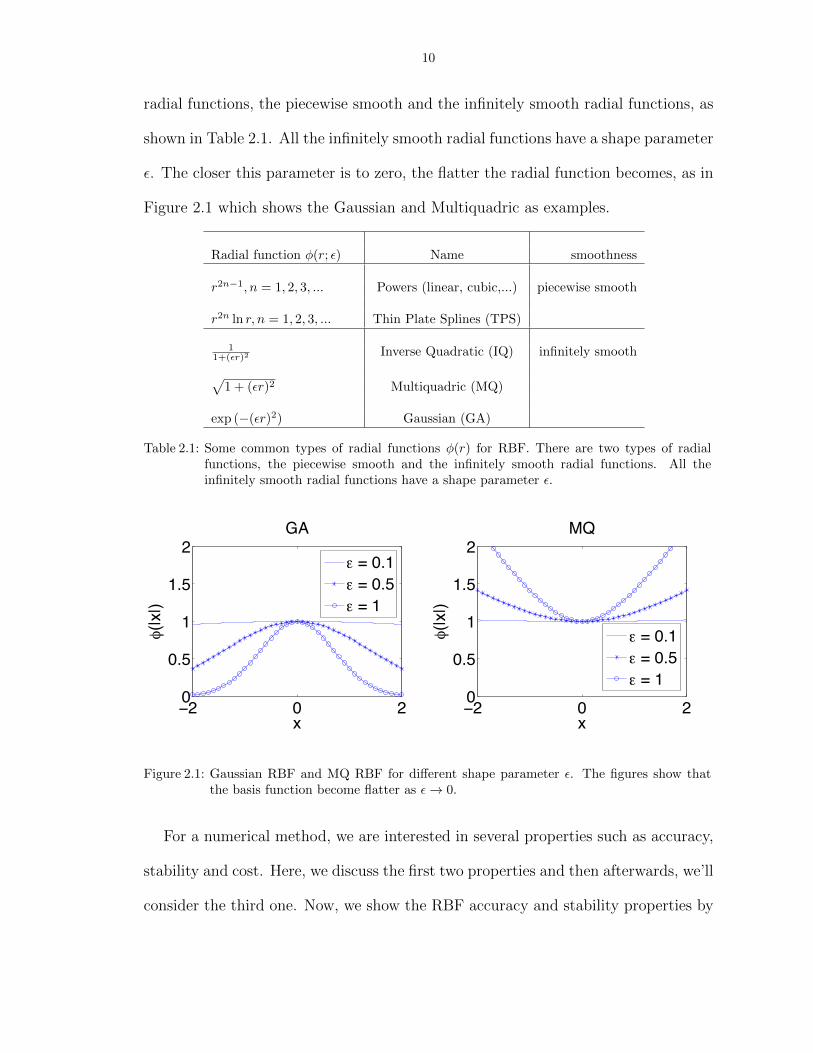
ε. The closer this parameter is to zero, the flatter the radial function becomes, as in

Figure 2.1 which shows the Gaussian and Multiquadric as examples.

Radial function φ(r; ε) Name smoothness

r2n−1, n = 1, 2, 3, ... Powers (linear, cubic,...) piecewise smooth

r2n ln r, n = 1, 2, 3, ... Thin Plate Splines (TPS)

11+(εr)2 Inverse Quadratic (IQ) infinitely smooth√

1 + (εr)2 Multiquadric (MQ)

exp (−(εr)2) Gaussian (GA)

Table 2.1: Some common types of radial functions φ(r) for RBF. There are two types of radialfunctions, the piecewise smooth and the infinitely smooth radial functions. All theinfinitely smooth radial functions have a shape parameter ε.

−2 0 20

0.5

1

1.5

2GA

x

!(|x

|)

" = 0.1" = 0.5" = 1

−2 0 20

0.5

1

1.5

2MQ

x

!(|x

|)

" = 0.1" = 0.5" = 1

Figure 2.1: Gaussian RBF and MQ RBF for different shape parameter ε. The figures show thatthe basis function become flatter as ε→ 0.

For a numerical method, we are interested in several properties such as accuracy,

stability and cost. Here, we discuss the first two properties and then afterwards, we’ll

consider the third one. Now, we show the RBF accuracy and stability properties by

11

using interpolation of Runge function,

(2.8) f(x) =1

1 + x2,

as an example on a one dimensional uniform grid. The basic features of this example

can be extended to high dimensional scattered data. The infinitely smooth radial

basis functions exhibit better approximation properties than the piecewise smooth

ones [34]. The accuracy of the infinitely smooth radial functions also depends on

the shape parameter ε and can be improved by increasing the flatness of the radial

function. Figure 2.2 shows Gaussian RBF interpolation for the Runge function (2.8)

when ε changes from 20 to 0.5. The left column shows both the function f(x) in

red and the interpolation function s(x) in blue circles. The right column shows

the absolute error |f(x) − s(x)|. Note that the error is decreasing from ε = 20 to

ε = 10 and ε = 1. The reason for this improvement is that when ε is small, the

basis functions are flat and have a lot of overlaps. However, the error increases as

ε decrease from ε = 1 to ε = 0.5. The reason is that the difference between each

basis function is small due to the flatness of the basis. The condition number shown

in Table 2.2 is large for small ε. This introduces a large computational error when

the RBF coefficients dj are computed by solving the linear system (2.7). Hence,

there is a trade-off between accuracy and conditioning for small ε and researchers

are showing great interest in this regime. Fornberg and his collaborators developed

“Contour Pade” method and “RBF-QR” method to overcome the ill-conditioning

and find RBF offers exponential convergence when ε is close to zero [36, 37].

2.3 Computational cost

Computational cost is another issue linked to using radial basis functions. Smooth

radial functions are global, thus the interpolation matrices A are dense. The system

12

−2 −1 0 1 20

0.2

0.4

0.6

0.8

1! = 20

x

f

(a)


−2 −1 0 1 20

0.1

0.2

0.3

0.4

x

erro

r

! = 20

(e)


−2 −1 0 1 20

0.2

0.4

0.6

0.8

1! = 10

x

f

(b)


−2 −1 0 1 20

0.002

0.004

0.006

0.008

0.01

0.012

x

erro

r

! = 10

(f)


−2 −1 0 1 20

0.2

0.4

0.6

0.8

1! = 1

x

f

(c)


−2 −1 0 1 20

0.2

0.4

0.6

0.8

1

1.2 x 10−4

x

erro

r

! = 1

(g)


−2 −1 0 1 20

0.2

0.4

0.6

0.8

1! = 0.5

x

f

(d)


−2 −1 0 1 20

0.005

0.01

0.015

0.02

x

erro

r

! = 0.5

(h)


Figure 2.2: Gaussian RBF approximation of the Runge function (2.8) on a uniform grid withN = 41for different ε. ((a)-(d)): f (red line) and interpolation function s(x) (blue ) versusx; ((e)-(h)): error versus x. Errors are decreasing first then increasing when ε changesfrom 20 to 0.5.

13

ε cond(A)

20 1.0758

10 5.8559

1 2.1038e+018

0.5 4.4236e+018

Table 2.2: Condition number of the matrix A when interpolating Runge function using GaussianRBF on a uniform grid with N = 41.

requires O(N3) operations to solve for the RBF coefficients dj by a direct method

such as LU factorization. Even though for iterative methods such as GMRES, the

solution involves matrix-vector multiplication with operation count O(N2) which

is still prohibitively expensive when N is large. However, there exist several fast

methods for performing the dense matrix-vector multiplication, which reduce the

operation count, such as the fast multiple method (FMM) [42, 43], treecode algorithm

[6, 7] and other choices such as multilevel summation [44, 59]. We will discuss this in

detail in Chapter Three. Next, we will be focus on the basic formulas for Gaussian

RBF.

2.4 Basic Formulas for Gaussian RBF

RBF is impressive for its ability to handle problems in scattered data and high

dimensions. However, it is not easy to do theoretical analysis of RBF in these

cases. Here and in the next sections, we will be focused on the Gaussian RBF for

a one dimensional evenly spaced grid, which can at least help us understand this

methodology. Here we rewrite the Gaussian RBF in a slightly different way,

(2.9) φ(x) ≡ exp(−[α2/h2]x2),

14

where α = εh and h is the grid spacing. More formally, we can always make the

change of variable

(2.10) X = x/h,

and the RBF approximation with grid spacing h in x is converted into one with

the same coefficients but unit grid spacing in X. One Reason for choosing the

Gaussian is that it is infinitely differentiable and such RBFs are more accurate than

RBFs of finite smoothness. In addition, Gaussian functions allow many theoretical

simplifications as illustrated below.

2.4.1 Computing the coefficients of an RBF expansion

RBF coefficients dj are usually obtained by solving a linear system. However,

there is another way to solve for the coefficients [34], [35]. Suppose we have a basis

function φ(X) and its Fourier transform is

(2.11) Φ(K) ≡∫ ∞−∞

φ(X) exp(iKX)dX.

Now consider a function f(X) approximated by RBFs on a uniform grid,

(2.12) f(X) =∞∑

j=−∞

djφ(X − j).

Then the RBF coefficients can be computed by,

(2.13) dj =1

2π

∫ π

−πψ(Y ) exp(ijY )dY,

where

(2.14) ψ(Y ) =

∑n=∞n=−∞ f(n) exp(−inY )∑n=∞n=−∞ φ(n) exp(−inY )

=

∑∞m=−∞ F (−Y + 2πm)∑∞m=−∞Φ(−Y + 2πm)

,

where F is the Fourier transform of the function f(X).

15

2.4.2 Poisson summation

There is an important relation between a function and its Fourier transform on a

evenly spaced grid.

Theorem II.1. (Poisson Summation) If g(X) and G(K) are a function and its

Fourier transform

G(k) ≡∫ ∞∞

g(X) exp(iKX)dX,(2.15)

g(X) = (1/2π)

∫ ∞−∞

G(K) exp(−iKX)dK,(2.16)

then for any positive constant q, it follows that

(2.17) q∞∑

n=−∞

g(qn) exp(inqx) =∞∑

m=−∞

G(x−m2π

q).

Furthermore, we have

∞∑n=−∞

(−1)ng(n) =∞∑

m=−∞

G([2m+ 1]π).(2.18)

Equation (2.17) shows a periodic function can be represented as a series of identical

but translated copies of the Fourier transform of the function g(x) [16].

2.5 Cardinal Function

One way to look into the intrinsic properties of RBFs and bypass both the ill-

conditioning and efficiency issues is to rearrange the RBF basis into the Lagrange

Cardinal basis,

Cj(xk) =

1, j = k,

0, j 6= k.

This gives an explicit, matrix-free solution to the interpolation problem,

(2.19) f(x) =n∑k=1

f(xj)Cj(x).

16

The cardinal function basis is much cheaper than the equivalent Gaussian RBF

interpolation, which forms a dense matrix. We developed an explicit expression for

the cardinal basis function for Gaussian RBF interpolation on a uniform grid [16].

2.5.1 Derivation

On a uniform grid, all Cj(x) are translations of a master basis function Cj(x) =

C(x − jh). All dependence on the (uniform) grid spacing h can be removed by the

change of variable X = x/h. The RBF approximation with grid spacing h in x is

converted into one with the same coefficients but unit grid spacing in X. Buhmann

[19] showed that, although there is no simple form for the cardinal function itself,

there is a remarkable formula for the Fourier Transform of an RBF cardinal function.

Define the Fourier Transform of the RBF function φ(x) by equation (2.11). Buhmann

proved that, not just for Gaussians but for RBF in general, the Fourier Transform

of C(X) is

(2.20) C(K) = Φ(K)/∞∑

m=−∞

Φ(K − 2πm).

For Gaussian RBFs, this yields

(2.21) C(K) =exp(−K2/(4α2))∑∞

m=−∞ exp(− (K−2πm)2

4π2

) =1∑∞

m=−∞ exp(−π2

α2m2)

exp(πmα2 K

) .We are more interested in the RBF properties for small α since the RBF approxima-

tion error is unacceptably big when α > 1 [16]. Hence, for small α, we approximate

the infinite series in (2.21) by three terms, the m = 0,−1, 1 terms, and obtain a

function whose inverse Fourier Transform can be explicitly computed from [41],

(2.22) Ca(K) =1

1 + 2 exp(−π2

α2

)cosh

(πα2K

) .

17

We have

(2.23)

C(X) ≈ α2

π√

1− 4 exp(−2π

2

α2

) sin

(α2X

πarccosh

(1

2exp

(π2

α2

)))1

sinh(α2X).

Neglecting terms of O(exp(−2π2/α2)) and using the lowest term in the arccosh series

(2.24) arccosh

(1

2exp(

π2

α2)

)≈ π2

α2− exp(−2

π

α2) + · · ·,

we have

(2.25) C(X) ≈ α2

π

sin(πX)

sinh(α2X).

It is obvious that

(2.26) C(0) ≈ α2

π

π cos(πX)

α2 cosh(πX)|X=0 = 1,

by L’Hospital’s rule. Figure 2.3 shows C(X) on the interval [−10, 10] with several

small values of α.

Figure 2.3: Cardinal function in equation (2.25) for different α. It equals one when X = 0 and zerofor the other integers.

The approximation can be written alternatively as

(2.27) C(X) ≈ α2

π

sin(πX)

sinh(α2X)=

α2X

sinh(α2X)sinc(X),

18

since sinc(X) = sin(πX)πX

. Note that limX→0X/ sinh(X) = 1, we have

(2.28) limα→0

α2

π

sin(πX)

sinh(α2X)= sinc(X),

which confirms that the RBF cardinal function reduces to the sinc function as α→ 0.

This cardinal function formula can be generalized to high dimensions.

Theorem II.2. (Uniform grid multidimensional cardinal functions)

On a uniform grid in any number of dimensions d, the Gaussian RBF cardinal func-

tion is the direct product of one-dimensional cardinal functions,

(2.29) Cd(x1, x2, , ..., xd) =d∏

m=1

C(xm).

The general cardinal function is just the translate of the master cardinal function,

i.e., in two dimensions

(2.30) C2jk(x, y) = C(x− jh)C(y − kh).

Proof. The direct product trivially satisfies the multidimensional cardinal function

condition. To show that this product is in the space spanned by d-dimensional Gaus-

sian RBFs, observe that by its very definition, the cardinal function is an exact sum

of basis functions. Thus, setting h = 1 for simplicity, C(X) =∑∞

j=−∞ pj exp(α2(X−

j)2) for some coefficients pj whose exact values are irrelevant. Therefore,

(2.31) C(d)(X1, X2, ..., Xd) =d∏

m=1

∞∑jm=−∞

pjm exp(−α2(Xm − jm)2).

The identity exp(a) exp(b) = exp(a+ b) implies that

(2.32)d∏

m=1

exp(−α2(Xm − jm)2) = exp(−α2||X −Xj||2).

Thus, each term is a d-dimensional RBF.

This concludes our discussion of RBF cardinal functions. Next, we will compare

the RBF with finite difference method using Fourier Analysis.

19

2.6 Comparison to Finite Differences Using Fourier Analysis

In addition to interpolation, we are interested in RBF approximation for deriva-

tives and solving PDEs. A finite difference (FD) formula can be obtained by differ-

entiating a polynomial interpolation and a standard way for assessing the accuracy

of differentiation formula is Fourier analysis. For RBF, we can treat it in the sim-

ilar way, that is, obtain an approximation by differentiating the RBF interpolant

s(x). Here, we will focus on Gaussian RBF and a basic Fourier mode exp(iKX) in

a one-dimensional unbounded domain with uniform grid distribution. We compare

the accuracy of this RBF derivative and FD derivative using Fourier analysis. We

start with the investigation of the Fourier mode exp(iKX).

2.6.1 Eigenvalues of the RBF difference operators for exp(iKX)

Differentiating exp(iKX) analytically yield

(2.33)d

dXexp(iKX) = iK exp(iKX).

Ignoring the imaginary factor “i”, denote the eigenvalue of the differential operator

by

(2.34) κexact(K) = K.

For a second-order centered FD approximation,

(2.35)

d

dXexp(iKX) ≈ 1

2(exp(iK(X + 1))− exp(iK(X − 1))) = i sinK exp(iKX),

that is,

(2.36) κFD2(K) = sinK.

20

Suppose we are looking for the difference formula that approximates the derivative

at X = 0 by

(2.37)df

dX(X = 0) ≈

M∑m=−M

ωmf(m).

Then for f(m) = exp(imX), assume ωm = −ωm which is true for all RBF and

centered FD approximation,

(2.38) κFD =M∑m=1

2ωm sin(mK).

Fornberg and Flyer [34], using the formula for dj given by (2.13) and (2.14), show

that for a radial basis function on a uniform grid, the eigenvalue is

(2.39) κRBF(K) =

∑∞m=−∞(K − 2πm)Φ(−K + 2πm)∑∞

m=−∞Φ(−K + 2πm),

where Φ is the Fourier transform of the basis function φ, as in (2.11). So for Gaussian

RBFs in particular,

(2.40) κGARBF(K) =

∑∞m=−∞(K − 2πm) exp(−(K − 2πm)2/(4α2))∑∞

m=−∞ exp(−(K − 2πm)2/(4α2)).

Note that, κRBF(K) is the ratio of two infinite series. It is hard to use this formula

directly but we can rewrite it using Jacobian theta function [2, 12],

(2.41) θ3(y = K/2; q = exp(−α2)) =

√π

α

∞∑m=−∞

exp

(−(K − 2πm)2

4α2

),

where θ3 is the usual Jacobian theta function and q is the ”elliptic nome” and

(2.42)d

dylog(θ3)(y; q) = 4

∞∑n=1

(−1)nqn

1− q2nsin(2ny).

21

We have

κGARBF(K) = −2α2ddKθ3(y = K/2; q = exp(−α2))

θ3(y = K/2; q = exp(−α2))(2.43)

= −2α2 d

dK

(log(θ(y = K/2; q = exp(−α2)))

)(2.44)

= 4α2

∞∑n=1

(−1)n+1 exp(−α2n)

1− exp(−2α2n)sin(nK)(2.45)

=∞∑n=1

(−1)n+1 2α2

sinh(α2n)sin(nK).(2.46)

Because the coefficients of the Fourier series for κ in equation (2.38) are also twice

the weights of the difference formula (2.37), we can truncate the above series (2.46)

to M terms to obtain the approximate eigenvalue of the Gaussian RBF when the

sum over all points on the grid is truncated to (2M + 1) terms:

(2.47) κGARBF(K,M) =M∑m=1

(−1)m+1 2α2

sinh(α2m)sinh(mK).

This means that the differentiation weights for RBF are given

(2.48) ωm = (−1)m+1 α2

sinh(α2m).

Hence from (2.46), the truncated RBF approximation for f = exp(iKX) is

(2.49)df

dX(X) ≈

M∑m=1

(−1)m+1 α2

sinh(α2m)(f(X +m)− f(X −m)) .

2.6.2 Numerical experiments

A differentiation formula is quite useless if it gives a poor approximation to the

differentiation eigenvalue. Somewhat arbitrarily, we have chosen an absolute error

of 0.05 as a threshold of minimum acceptability, and graphed the performance of

truncated Gaussian RBF differentiation formulas in the K−α plane for four different

stencil widths in Figure 2.4. It shows that the area in which the error is less than

0.05 is increasing as M increases. However, the results are unsatisfactory for α < 1,

22

which is the regime we are interested in for RBF interpolation. For example, the

area that the error is less than 0.05 is quite small even for a 9 point-stencil.

Figure 2.4: The shaded regions show where the absolute error in the eigenvalue of the first deriva-tive, K − κ(K;M), is smaller than 0.05 for four different values of M as a function ofα.

Figure (2.5 plots the ratio of the finite difference errors to the RBF errors in the

eigenvalue of the first derivative κ(K) for nine-point, seventeen-point and thirty-

three point stencils. The pattern is quite consistent between different orders M :

the RBF method is better for K near the aliasing limit, but much worse by a huge

factor for small K. For the thirty-three point stencil, the region of RBF superiority

lies wholly in the right one-third of the wavenumber range. In realistic calculations,

these Fourier components would likely be corrupted by aliasing error and in fact are

completely eliminated by a dealiasing filter of the sort common in fluid mechanics

[15].

These numerical tests show that the truncated RBF approximation (2.49) which

23

(a) (b)

(c)

Figure 2.5: Finite difference error divided by Gaussian RBF error in the eigenvalue of the firstderivative versus K for M = 4, 8, 16, which is a stencil of nine, seventeen and thirtythree points with different α. The thick dashed horizontal line is where the ratio is one:the radial basis function method is better whenever the ratio is above this line, and thefinite difference is better whenever the curve is below this dashed line. The thin dottedline marks the right one-third of the spectrum which would be removed by a dealiasingfilter in a hydrodynamics computation.

is obtained using the similar idea as FD is inferior than FD in terms of approximating

the Fourier mode exp(iKX).

In this chapter, we give an introduction to the RBF method, including its back-

ground, advantage and related problems. The most significant property of RBF ap-

proximation is the trade-off between exponential convergence and ill-conditioning.

We also present an RBF cardinal function for Gaussian in one dimensional un-

bounded evenly spaced grid. At the end, we compare the accuracy of RBF method

24

and Finite Differences method in terms of Fourier analysis. We find that the trun-

cated Gaussian RBF method is inferior to the FD for differentiating the function

f(X) = exp(iKX), where K is the wavenumber.

CHAPTER III

Fast Treecode for Evaluating RBFs

3.1 Introduction

As we mentioned in Chapter Two, one of the major concerns in the application of

RBFs is the computational cost. There are two expensive steps in RBF approxima-

tion. The first step is to calculate the RBF coefficients dj by solving a linear system

(2.7). The operation count for solving a dense linear system by LU decomposition is

O(N3). Other choices like iterative methods such as GMRES, involve matrix-vector

multiplication with operation count O(N2). The second step is to evaluate the RBF

summations,

(3.1) s(xi) =N∑j=1

djφ(xi − yj), i = 1 : M,

where yj are interpolation points and xi are evaluation points. Note that compared

to (2.6), equation (3.1) is rewritten with a slight abuse of notation. Equation (3.1)

can be viewed as a matrix-vector multiplication with operation count O(NM). Both

steps are prohibitively expensive when N,M are large. Hence, the bottleneck of the

computational cost is the matrix-vector multiplication. There are several existing

fast evaluation algorithms including the treecode algorithm of Barnes and Hut [7]

and the Fast Multipole Method (FMM) of Greengard and Rokhlin [43] and others

for different RBF kernels [44, 59, 11]. Some of the work in this chapter is published

25

26

in [53]. For a given accuracy, the treecode requires O(N logN) operations and the

FMM requires O(N) operations. Both Treecode and FMM divide the particles into

a hierarchy of clusters having a tree structure and they approximate particle-cluster

or cluster-cluster interactions instead of particle-particle interactions. The Treecode

algorithm is more advantageous in terms of algorithm complexity and memory usage.

For simplicity, we consider speeding up the N-body system

(3.2) s(xi) =N∑j=1

djφ(xi − xj), i = 1 : N,

by treecode algorithm. That is, target points are the same as source points. Note

that it is not a restriction for the treecode.

3.2 Build Tree

There are two ways to construct a hierarchical tree. The first choice is using the

maximum number of levels (L). A complete tree is constructed as follows:

1. The collection of particles is enclosed with a rectangular box, which becomes

the root cell of the tree. Set the level of current cell p1 to be l = 0;

2. Subdivide current cell pi into subcells (children) by bisecting pi in the two/three

coordinate directions. The result is four children in two dimensions and eight

children in three dimensions. Label the level number of each child l = l + 1;

3. If l is less then L, apply step 2 to each child of pi.

Figure 3.1 shows a tree for L = 3 in 2 dimensions. Note that every leaf is in the

same level. a leaf is a cell which doesn’t have children.

The other way to construct a tree ensures that every leaf contains fewer particles

than a parameter N0. The tree is constructed as follows:

27

L = 0 L = 1

L = 2 L = 3

Figure 3.1: Complete hierarchical tree structure in two dimension for 4 levels. Level = 0 is alsocalled the root cluster.

1. The collection of particles is enclosed with a rectangular box, which becomes

the root panel p1 of the tree;

2. If the current panel pi contains fewer than N0 particles then exit. The panel is

a leaf of the tree.

3. Otherwise, subdivide current cell pi into subpanels (children) by bisecting pi in

the coordinate directions and apply step 2 to each children.

Figure 3.2 shows the structure of tree for N0 = 1. Compare to the complete tree,

this version is more adapted to the distribution of particles and each leaf can be at

a different level of the tree.

We notice that both L and N0 controls the depth of the tree. They affect the

performance of the algorithm. If N0 is too small, then the tree will have many levels,

leading to a large memory requirement. However, if N0 is too large, then the tree

28

L = 0 L = 1

L = 2 L = 3

Figure 3.2: Adaptive hierarchical tree structure in two dimensions for N0 = 1, where N0 is themaximum number of particles in a leaf.

consists of cells having large spatial dimensions that evaluate many particle-particle

interaction by direct summation and the efficiency may be affected.

3.3 Particle-Cluster Interaction

In this section, we will introduce the particle-cluster interaction. Barnes and

Hut (1986) [7] presented a hierarchical treecode method for calculating the force on

N bodies with operation count O(N logN), where particle-cluster interactions were

performed by approximating the cluster as if all particles in the cluster are located

at the cluster’s center of mass. A drawback of this approximation is its low accuracy.

The Fast Multipole Method of Greengard and Rokhlin (1987) [43] overcame this

obstacle by using a series expansion to approximate particle-cluster interactions to

any specified tolerance. They also introduced cluster-cluster interactions by expand-

ing the far-field approximation into a local near-field expansion for rapid evaluation

29

at multiple target points. The operation account is O(N). However the algorithm

is very complicated. Lindsay and Krasny (2001) [58] developed a Barnes-Hut type

treecode with Taylor series as far-field expansion, which improved the accuracy of

the algorithm and requires O(N logN) operations. Here we will focus on a treecode

with Cartesian Taylor series as far field expansion. One of the major steps of the

treecode algorithm is to find a well-separated particle-cluster interaction list. But

how is a well-separated particle-cluster interaction defined?

3.3.1 Well-separated particle-cluster interaction list 1

Points x are said to be well-separated from cluster p if x are separated from the

panel p by at least the diameter of p [10]. For the complete tree structure, Figure

3.3 shows a way to find a well separated particle-cluster interaction list. Suppose the

target points are in the red cell, then the white cells are the neighbors of the red cell,

they are in the same level and share a edge. The direct summation will be performed

between the particles in the target panel and the particles in the neighbor panels.

The blue cells are the well separated ones. Notice that some of them are in the same

level of the target panel and some are in the parents’ level of target cell. Since the

level number of parents is always smaller than the level number of the children, it is

better to choose smaller level clusters as long as they are well-separated.

3.3.2 Well-separated particle-cluster interaction list 2

For the adaptive tree structure shown in Figure 3.2, Barnes and Hut present the

following approach (Figure 3.4(a)). For a given target point, start from the root

panel in the tree.

1. evaluate the distance between the target point and the center of the current

panel, denote as R, the radius of the current panel , denote as r;

30

Figure 3.3: Example of neighbors and well separated panels for a complete tree. The target pointsare in the red cell, the white cells are the neighbors and the blue cells are the wellseparated cells of the red cell.

2. if the ratio r/R is less than a user specified number (MAC) θ, the current panel

is a well-separated panel for the target point;

3. otherwise, if current panel is a leaf, then it is a panel to which direct summation

will be applied, otherwise apply step 2 for each children of current panel.

Barnes [6] presented a modified treecode. Instead of defining an interaction list for

each target point, he built an interaction list for each leaf. All the particles in the

same leaf share the same interaction list, Figure 3.4(b). For Barnes [6], the target

cells are the leafs of the tree and R is the distance between the center of the target

cell and current cell.

Experiments show that the performance of Barnes [6] is better than Barnes and

Hut [7] and the neighbor idea in the complete tree shown in Figure 3.3. We use

Barnes [6] in our implementation of the treecode algorithm.

For the leaf panels that don’t satisfy the MAC condition, direct summation will

be applied.

31

(a) (b)

Figure 3.4: Particle cluster interaction when r/R < θ, where r is the radius of the cluster and θ isMAC number. (a): Barnes and Hut [7]; R is the distance between x and the center ofthe cluster yC ; (b): Barnes [6], R is the distance between the centers of the two clusters.

3.3.3 Far field expansion

This section explains the far-field expansion for a well-separated particle-cluster

interaction. The flow chat for the entire treecode will be presented later. Using

Cartesian coordinates and standard multi-index notation, equation (3.2) yields:

s(xi) =N∑j=1

djφ(xi − xj)(3.3)

=∑C

∑yj∈C

djφ(xi − yj)(3.4)

=∑C

∑yj∈C

dj

∞∑||k||=0

1

k!Dk

yφ(xi − yC)(yC − yj)k(3.5)

=∑C

∞∑||k||=0

1

k!Dk

yφ(xi − yC)∑yj∈C

dj(yC − yj)k(3.6)

≈∑C

p∑||k||=0

ak(xi − yC)mk(C),(3.7)

where C are far interaction cells for target point xi. The equation (3.5) shows that

a far-field expansion of the basis φ is taken at yC , which is the center of the cell C.

The k = (k1; k2; k3) is an integer multi-index with all ki > 0 in three dimensions,

32

||k|| = k1 + k2 + k3, k! = k1!k2!k3!. We call

(3.8) ak(xi,yC) =∞∑

||k||=0

1

k!Dk

yφ(xi − yC)

the kth order Taylor coefficient of φ(x− y) at y = yC and

(3.9) mk(C) =∑yj∈C

dj(yC − yj)k

is the kth moment of cluster C about its center yC . Note that in (3.6), we change

the order of the summation. The cluster moment (3.9) doesn’t depend on the target

points. (it depends only on the cluster), so it can be calculated once after the tree

is constructed.

3.4 Recurrence Relation for Taylor Series

For the algorithm to be computationally efficient, it is necessary to rapidly com-

pute the Taylor coefficients ak(xi,yC) = 1k!Dk

yφ(xi,yC) in (3.8). We derive the

recurrence relations for several radial basis functions in Table 2.1. Note that here

we use a slightly different notation for the basis function, that is, instead of using

ε as shape parameter as shown in Table 2.1, We use c ∼ ε−1. For example, the

Multiquadric is φ(x− y) =√

(x− y) + c2.

3.4.1 Multiquadric

Theorem III.1. The Taylor coefficients ak(x,y) = a(k1,k2,k3)(x,y) of the Multi-

quadric basis function φ(x− y) =√|x− y|2 + c2 satisfy the recurrence relation

(3.10) ||k||(|x−y|2 +c2)ak− (2||k||−3)3∑i=1

(xi−yi)ak−ei +(||k||−3)3∑i=1

ak−2ei = 0

33

for ||k|| ≥ 1, where a0 = φ(x,y), ak = 0 if any ki < 0, ei is the Cartesian unit

vectors and

k − ei =

(k1 − 1, k2, k3), i = 1,

(k1, k2 − 1, k3), i = 2,

(k1, k2, k3 − 1), i = 3.

Proof. The Multiquadric basis function φ(x,y) =√|x− y|2 + c2 satisfies the differ-

ential equation

(3.11) (x1 − y1) +√|x− y|2 + c2Dy1φ = 0

Applying the operator Dk1−1y1

and using Leibniz’s rule for differentiating a product

we obtain

(3.12) (|x−y|2 + c2)Dk1y1φ+ (3− 2k1)(x1− y1)Dk1−1

y1φ+ (k1− 3)(k1− 1)Dk1−2

y1φ = 0.

Next we apply Dk2y2Dk3y3

and substitute the definitions of ak to obtain

(3.13) k1(|x−y|2+c2)ak−2k1

3∑i=1

ak−ei+3(xi−yi)ak−e1+k1

3∑i=1

ak−2ei−3ak−2e1 = 0.

Equation (3.13) is a recurrence relation for ak in which the index 1 plays a special role.

Similar equations can be obtained for indices 2 and 3. Summing these equations, we

obtain (3.10).

3.4.2 Gaussian

Theorem III.2. The Taylor coefficients ak of Gaussian basis function φ(x− y) =

exp (−|x− y|2/c2) satisfy the recurrence relation

(3.14) c||k||ak − 23∑i=1

(xi − yi)ak−ei + 23∑i=1

ak−2ei = 0.

34

3.4.3 Inverse multiquadric

Theorem III.3. The Taylor coefficients ak of Inverse Multiquadric basis function

φ(x− y) = 1√|x−y|2+c2

satisfy the recurrence relation

(3.15) ||k||(|x−y|2 +c2)ak+(1−2||k||)3∑i=1

(xi−yi)ak−ei +(||k||−1)3∑i=1

ak−2ei = 0.

We omit the proofs of (3.14) and (3.15) here since they are almost the same as the

proof of Multiquadric recurrence relation (3.10). With the help of these recurrence

relations, the Taylor coefficients ak can be calculated very efficiently. Figure 3.5

shows how recurrence relations work in two dimensions, i.e. k = (k1, k2). Suppose

we need to calculate the a(k1,k2) at the blue dot position, we only need the value of

a at four red dot positions which have already been calculated and stored.

Figure 3.5: Example of 2d stencils for recurrence relation. Taylor coefficients at blue point onlydepends on the coefficients at four red points.

3.5 Treecode Algorithm

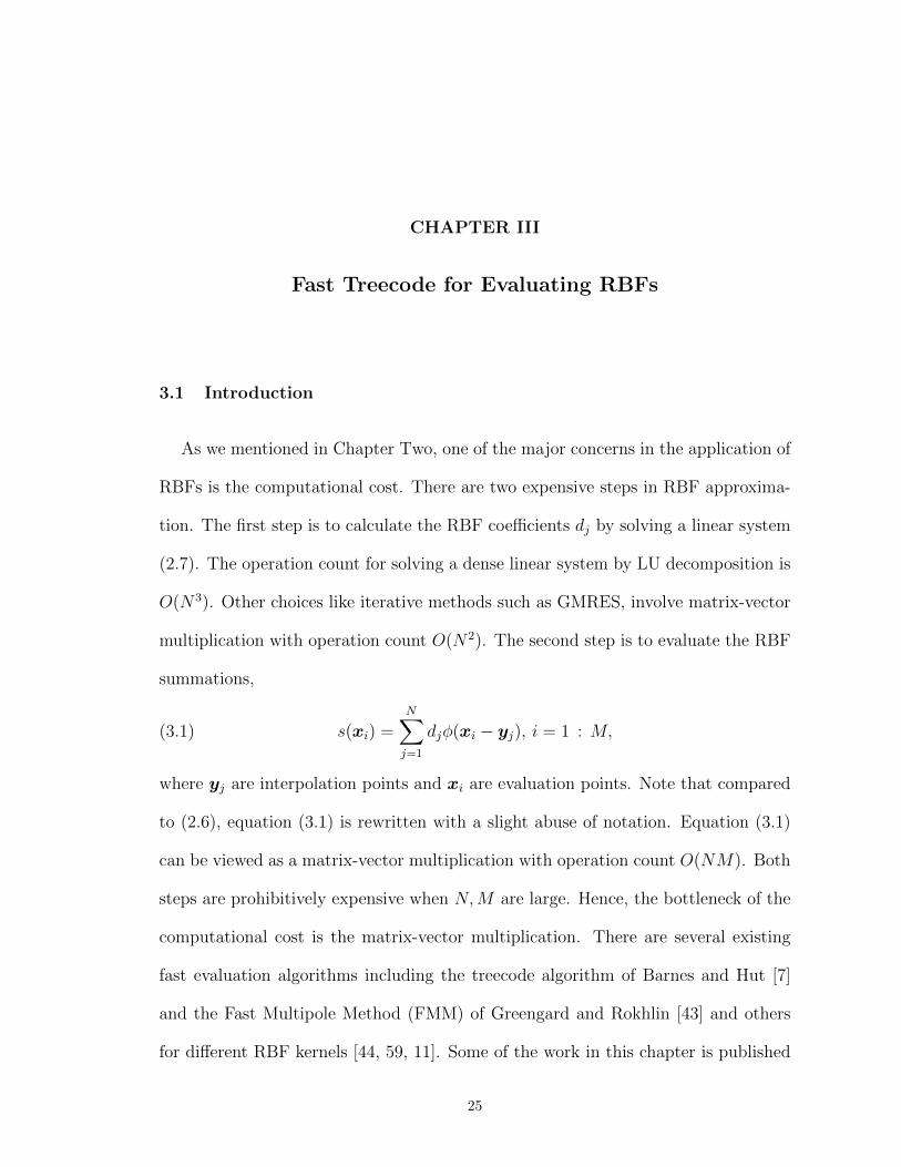
Figure 3.6 is the flowchart for Barnes and Hut [7] treecode algorithm. The main

function (3.6(a)) starts with inputting RBF nodes xi, coefficients dj, treecode param-

eters, which include the MAC number θ, Taylor approximation order p and maximum

35

leaf size N0. θ is the number which controls where we will use particle-cluster in-

teraction. Then we construct the tree according to the position of RBF nodes xi.

Next, for every particle, starting from the root cluster, compute the particle-cluster

interaction. The role of the subroutine compute interaction (3.6 (b)) is to compute

the particle-cluster interaction. If the current target particle and current cluster are

well separated, then calculate the interaction using Taylor approximation, otherwise,

check the children of the current cluster to see whether they are well separated from

target point. There is a recursive call in the subroutine which makes the program

easy to implement.

(a) (b)

Figure 3.6: Flowchart of Barnes and Hut [7] treecode algorithm. (a) main function and (b) subrou-tine compute interaction. Note that there is a recursive call in the subroutine.

3.6 Cartesian Taylor Treecode for Multiquadric RBF

As we mentioned in Chapter Two, the shape parameter ε plays an important role

in RBF approximation. Since c ∼ 1/ε, c controls the shape of the basis functions

also. When c is large, the basis functions overlap, the RBF approximation shows

exponential convergence but on the other hand, the difference between each row of

36

the RBF matrix Ai,j = φ(xi − xj) is small, the condition number of A is large.

Researchers in this field are very interested in large c regime. Here, we present a

treecode for evaluating Multiquadric RBF using Taylor series. We show that for the

MQRBF case, the Taylor series converges for all RBF parameter values c > 0, in

contrast to the Laurent series which converges for a limited range of c as presented

in literature [10, 22].

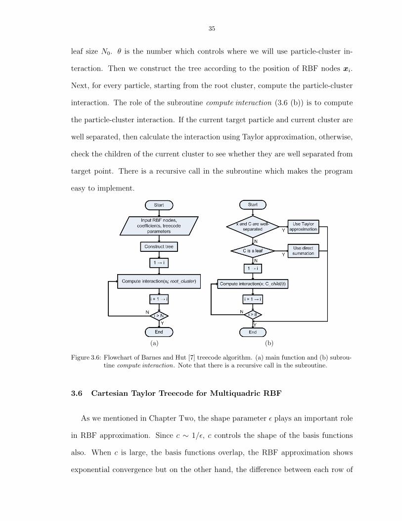
3.6.1 Far field expansion for multiquadric in 1D

The multiquadric function in 1D is:

(3.16) φ(x− y) =√

(x− y)2 + c2.

Beatson and Greengard [10] proposed the Laurent series in x for (3.16)

(3.17) φ(x− y) =√|x− y|2 + c2 = sign(x) ·

(x− y +

c2

2x+c2y

2x2+ · · ·

)Note that in the complex x plane for φ(x− y), the two branch points are y + ic and

y − ic. The shaded area outside of the unit circle in Figure 3.7 is the convergence

area for the Laurent series. The convergence criterion for (3.17) is

Figure 3.7: Schematic showing branch points, branch cuts, and domain of convergence (shaded)for far-field expansions of φ(x) given in (3.16); (a) the Laurent series (3.17) convergesoutside a disk in the x-plane; (b) the Taylor series (3.19) converges inside a disk in they-plane. As c increases, the shaded region in (a) becomes smaller and the shaded regionin (b) becomes larger.

(3.18) ρ1 ≡√y2 + c2

|x| < 1.

37

Note that in (3.18), the RBF parameter c is in the numerator. Assuming |x| > |y|,

the convergence criterion (3.18) restricts the value of c that can be used. Now,

consider the Multiquadric (3.16) as a function of y and x is a parameter. Taking

Taylor series with respect to y at y = 0, we have

(3.19) φ(x− y) = xc −xy

xc+c2y2

2x3c

+c2xy3

2x5c

+c2(4x2 − c2)y4

8x7c

+ · · · ,

where xc =√x2 + c2. Then the Multiquadric (3.16) has two branch points y = x+ic

and y = x− ic in the complex y plane. Figure 3.7 (b) shows the convergence area for

Taylor series (3.19) is the shaded area inside the circle. The convergence criterion

for (3.19) is

(3.20) ρ2 ≡|y|√x2 + c2

< 1.

Note that the RBF parameter c in (3.20) is in the denominator. So for |x| > |y|, the

series (3.19) is uniformly converging for c > 0. Furthermore, the convergence rate

improves as c increases.

Here we consider an example from in one space dimension [10]. Figure 3.8 shows that

a cluster C is a line interval with radius h, all particles yi ∈ C satisfy |yi| < h. All

evaluation points are |xi| > 3h. Evaluation points and the cluster C are separated

by at least one diameter of C. Let c = h as in [10], the convergence rates are

(3.21) ρ1 = maxi,j

√y2j + c2

|xi|≤√h2 + h2

3h=

√2

3= 0.47,

(3.22) ρ2 = maxi,j

|yj|√x2i + c2

≤ h√9h2 + h2

=1√10

= 0.32.

We can see that ρ2 < ρ1, which means that the Taylor series (3.19) converges faster

than the Laurent series (3.17). Again, increasing c accelerates the convergence rate

of the Taylor series (3.19).

38

Figure 3.8: Example in 1D from [10] showing a cluster C of nodes satisfying |yj | ≤ h and well-separated evaluation points satisfying |xi| ≥ 3h.

3.6.2 The generalized multiquadric in muti-D

Generalized multiquadric is defined:

(3.23) φ(x− y) = (|x− y|2 + c2)ν/2,

where x,y ∈ Rd and ν ∈ R is an odd number. As we did for the one dimension case,

there is a Laurent series in x,

(3.24) φ(x− y) = (|x− y|2 + c2)ν/2 =∞∑l=0

P(ν)l (|y|2 + c2,−2〈x,y〉, |x|2)

|x|2l−ν ,

where P(ν)l is a multivariate polynomial

(3.25) P(ν)l (b1, b2, b3) =

l∑j=b l+1

2c

(ν/2

j

)(j

l − j

)b2j−l

2 (b1b3)l−j

for l ≥ 0 and P(ν)l (b1, b2, b3) = 0 for l < 0 [22]. The Laurent series (3.24) converges

for |x| >√|y|2 + c2. There is also a Taylor series in x

(3.26) φ(x− y) = (|x− y|2 + c2)ν/2 =∞∑l=0

P(ν)l (|x|2,−2〈x,y〉, |y|2 + c2)

(|y|2 + c2)(2l−ν)/2,

which converges for |x| <√|y|2 + c2. Cherrie, Beatson and Newsam (2002) [22]

developed a FMM using the Laurent series (3.24) for the far-field expansion and the

Taylor series (3.26) for the near-field expansion.

We are interested in a Taylor series in y. Let us interchange x and y in Taylor

series (3.26) and have

(3.27) φ(x− y) = (|x− y|2 + c2)ν/2 =∞∑l=0

P(ν)l (|y|2,−2〈x,y〉, |x|2 + c2)

(|x|2 + c2)(2l−ν)/2,

39

which converges for |y| <√|x|2 + c2. This is a Taylor series in y. We rewrite it by

collecting like powers of y to have a standard Taylor expansion with respect to y at

y = 0

(3.28) φ(x− y) = (|x− y|2 + c2)ν/2 =∞∑

||k||=0

1

k!Dkφ(x) (−y)k,

where k = (k1, . . . , kd), ki ≥ 0 are integers, ||k|| = k1 + · · · + kd, k! = k1! · · · kd!,

yk = yk11 · · · ykdd , and Dk = Dk11 · · ·Dkd

d .

The far-field expansion will be applied for well separated particle cluster interac-

tions. We take the Taylor expansion at the center of cluster yC ,

(3.29) φ(x− y) = (|x− y|)ν/2 =∞∑

||k||=0

1

k!Dkφ(x− yC) (−(y − yC))k,

which converges for |y − yC | <√|x− yC |2 + c2. Then as we did before

s(xi) =N∑j=1

djφ(xi − xj)(3.30)

=∑C

∑yj∈C

djφ(xi − yj)(3.31)

=∑C

∑yj∈C

dj

∞∑||k||=0

1

k!Dk

yφ(xi − yC)(yC − yj)k(3.32)

=∑C

∞∑||k||=0

1

k!Dk

yφ(xi − yC)∑yj∈C

dj(yC − yj)k(3.33)

≈∑C

p∑||k||=0

ak(xi − yC)mk(C)(3.34)

where ak are kth order Taylor coefficient and mk are the cluster moments as men-

tioned in section 3.3.3. In section 3.4, we derived the recurrence relation for Taylor

coefficients for multiquadric for ν = 1 and d = 3. Here is the recurrence relation for

all odd ν ∈ R,

(3.35)

ak+2(||k|| − 1)− ν

||k||(|xi − yC |2 + c2)

3∑j=1

((xi)j−(yC)j)ak−ej+||k|| − 2− ν

||k||(|xi − yC |2 + c2)

3∑j=1

ak−2ej = 0.

40

The proof is similar to (3.10). For ||k|| = 0, 1 the coefficients ak are computed

explicitly and then (3.10) is used to compute the coefficients for ||k| ≥ 2.

Next we compare the errors in the Laurent series and the Taylor series for a

particle-cluster interaction in the case ν = 1, d = 3, in Figure 3.9. The particle

(red) is located at the origin in R3, x = 0, and the cluster C consists of N = 103

nodes distributed randomly in the cube [0.75, 1]3. They are well separated since

the distance between the cluster and the particle is larger than the diameter of the

cluster. The RBF coefficients are set to di = 1 as in [22]. The error is defined by

(3.36) E1 =|s(x, C)− s(x, C)|

|s(x, C)| ,

where s(x, C) is the exact particle-cluster interaction(3.2) and s(x, C) is the ap-

proximation obtained by truncating the expansion for φ(xi − yj) using the Laurent

series (3.24) or the Taylor series (3.29). For each approximation, the necessary series

coefficients were computed using the recurrence relations discussed above.

Figure 3.10 shows the error as a function of the RBF parameter c and order p,

for 10−3 ≤ c ≤ 103 and p = 0 : 2 : 10. As noted above, the Laurent series converges

on an interval 0 ≤ c ≤ c and diverges for c > c, while the Taylor series converges

for all c ≥ 0. For some special values of p and c, the error drops to zero; this occurs

near c = 10−1 for the Laurent series and near c = 1 for the Taylor series. For small

values of c, the two series have comparable errors. For a given order p, the rate

of convergence of the Taylor series improves as c → ∞. These results confirm the

favorable convergence properties of the far-field Taylor series (3.29).

3.6.3 Treecode performance

The treecode was implemented in the C programming language and the computa-

tions were performed on an Intel Pentium M processor (1.5 GHz, 768 MB RAM,1024

41

Figure 3.9: A well separated particle-cluster interaction example for testing the convergence ofLaurent expansion (3.24) and Taylor expansion (3.26).

Figure 3.10: Error (3.36) in a particle-cluster approximation with one evaluation point at the originin R3 and a cluster of N = 103 random nodes in the cube [0.75, 1]3; ν = 1, d = 3. Theerror is plotted as a function of the RBF parameter c and order p, for 10−3 ≤ c ≤ 103

and p = 0 : 2 : 10. (a) Laurent series (3.24), (b) Taylor series (3.29).

KB level 2 cache). Memory usage was obtained using the performance counter tool

in the Windows operating system.

We present results using the treecode for two test cases in 3D. In the first case we

consider random nodes in a unit cube and in the second case the nodes were projected

radially from the cube to the surface of a unit sphere Figure 3.11. One motivation

for considering the sphere is the growing interest in RBF methods for geophysical

fluid flow [32] and our Lagrangian method application on sphere (Chapter Five and

42

Figure 3.11: N random points in a cube (left) and on the surface of a sphere.

Chapter Six). In both test cases, the RBF coefficients were set to di = 1, as in [22],

and the RBF parameter was set to c = 10−1. The relative error is defined by

(3.37) E2 =

(N∑i=1

|s(xi)− s(xi)|2/ N∑

i=1

|s(xi)|2)1/2

,

where s(xi) is the exact value (3.2) obtained by direct summation and s(xi) is the

treecode approximation.

3.6.4 Random nodes in a cube

First we present results using N = 216K nodes for order p = 0 : 2 : 10 and MAC

parameter θ = 0.2, 0.5, 0.8, with maximum leaf size N0 = 200. Table 3.1 presents

the data. As expected, for a given value of θ, increasing order p yields smaller error

and larger CPU time. Similarly, for a given value of p, decreasing MAC parameter

θ also yields smaller error and larger CPU time. Figure 3.12 displays the data as

a scatter plot. The data points for each θ are connected by a line and p increases

moving from right to left on each line. The lower envelope of the data gives the most

efficient choice of parameters (p, θ) to attain a given error. For example, errors in

the interval [10−6, 10−1] are computed with least CPU time using θ = 0.8. We set

θ = 0.8 in the remainder of this work.

43

Table 3.1: Random nodes in a cube, the treecode error (3.37) and CPU time (sec) are given forsystem size N = 216K, RBF parameter c = 10−1, order p = 0 : 2 : 10, MAC parameterθ = 0.2, 0.5, 0.8, maximum leaf size N0 = 200.

treecode error (3.37) CPU time (sec)

p θ = 0.8 θ = 0.5 θ = 0.2 θ = 0.8 θ = 0.5 θ = 0.2

0 3.379e-2 1.376e-2 2.213e-3 0.9 3.2 259.0

2 5.835e-5 1.292e-5 3.081e-7 7.8 30.2 470.1

4 2.014e-5 1.336e-6 2.711e-9 15.7 55.8 798.1

6 2.149e-6 8.761e-8 3.065e-11 33.5 119.3 1444.0

8 5.805e-7 5.461e-9 4.890e-13 63.0 308.9 2522.5

10 1.850e-7 6.107e-10 2.220e-14 115.7 684.4 4304.4

Next we vary the problem size. Figure 3.13 presents the error (3.37) as a function

of order p for problems of size N = 103, 203, . . . , 1003. The maximum leaf size was

N0 = 200, except for the two largest systems (N = 903, 1003) for which N0 = 400.

Figure 3.13 shows that the error is almost independent of system size N , and for a

given value of N , the error decreases with increasing order p. Figure 3.14 presents

the corresponding CPU time, showing that the treecode CPU time is consistent with

O(N logN) scaling and that the treecode is faster than direct summation except for

small system size N and large order p.

Figure 3.15 plots the amount of memory used by the treecode as a function of

system size N for order p = 0 : 2 : 10. The memory used by direct summation is also

shown. The treecode uses arrays of size O(p3) to store cluster moments and Taylor

coefficients, and hence it requires more memory as the order p increases. For low

order p, the treecode memory usage is a small multiple of the memory required by

direct summation. For high order p, the treecode memory usage becomes irregular

and this is why the maximum leaf size was changed from N0 = 200 to N0 = 400 for

the two largest systems. It is likely that the treecode memory usage can be reduced

44

Figure 3.12: Random nodes in a cube, scatter plot of CPU time and error (3.37), data from Ta-ble 3.1, system size N = 216K, order p = 0 : 2 : 10 (increasing from right to left),MAC parameter θ = 0.2 (,black), θ = 0.5 (∗,red), θ = 0.8 (4,blue), RBF parameterc = 10−1, maximum leaf size N0 = 200. The lower envelope of the data gives the mostefficient choice of parameters (p, θ) to attain a given error.

by further tuning, but even so, for the largest system considered here (N = 106)

and the highest order (p = 10), the treecode used approximately only three times as

much memory as direct summation.

3.6.5 Random nodes on a sphere

Table 3.2 compares two test cases, random nodes in a cube and on a sphere, for

problems of varying size, using a representative set of parameter values, θ = 0.8, p =

6. We record results for the treecode and direct summation. Note that the direct

sum CPU time and memory usage depend on the system size N , but not on the

node distribution, so these values are the same for the two test cases. Next note

that the treecode error is essentially the same for the two node distributions, while

the treecode CPU time and memory usage are slightly higher for the sphere than

for the cube, with approximately a 10% penalty in CPU time and a 33% penalty in

45

Figure 3.13: Random nodes in a cube, treecode error (3.37) plotted as a function of system sizeN = 103, 203, . . . , 1003, order p = 0 : 2 : 10, MAC parameter θ = 0.8, RBF parameterc = 10−1, maximum leaf size N0 = 200 except N0 = 400 for N = 903, 1003.

Figure 3.14: Random nodes in a cube, treecode CPU time in seconds, same parameters as in Fig-ure 3.13 caption, ds denotes direct sum.

46

Figure 3.15: Random nodes in a cube, treecode memory usage in MB, same parameters as inFigure 3.13 caption, ds denotes direct sum.

memory usage for the largest system N = 1000K. It is likely that greater efficiency

can be gained in the sphere test case, for example by shrinking the clusters [57] or

by spherical panel clustering. The overall favorable performance of the treecode in

the sphere test case arises from the adaptive nature of the tree structure, which has

been noted before [7].

In this chapter, we present a fast Cartesian treecode for evaluating RBFs effi-

ciently. The method applies a divide and conquer strategy and uses particle-cluster

interactions in place of particle-particle interactions. Taylor approximation is applied

for the far-field expansion. For multiquadric RBFs, φ(x) =√x2 + c2, the Laurent

series presented in the literature converges only for a limited range of c, but the Tay-

lor series converges for all c ≥ 0. The treecode algorithm reduces the computational

cost from O(N2) to O(N logN) operations, where N is the size of the system.

47

Table 3.2: Random nodes in a cube and on a sphere, tc denotes treecode and ds denotes direct sum,CPU time in seconds and memory in MB, RBF parameter c = 10−1, maximum leaf sizeN0 = 200 except N0 = 400 for N = 1000K, order p = 6, MAC parameter θ = 0.8.

N → 8K 64K 216K 512K 1000K

cube

error (tc) 7.5e-6 2.7e-6 2.1e-6 2.2e-6 2.2e-6

CPU (tc) 0.7 8.5 33.5 84.4 165.9

CPU (ds) 1.5 95.7 978.8 5479.0 21888.2

memory (tc) 1.0 7.1 29.9 50.0 76.7

memory (ds) 0.5 2.8 8.8 20.7 40.2

sphere

error (tc) 4.0e-6 2.6e-6 2.6e-6 2.4e-6 2.1e-6

CPU (tc) 0.7 8.7 34.1 88.5 180.7

CPU (ds) 1.5 95.7 978.8 5479.0 21888.2

memory (tc) 1.0 9.1 29.6 72.0 101.2

memory (ds) 0.5 2.8 8.8 20.7 40.2

CHAPTER IV

Barotropic Vorticity Equation

4.1 Introduction

We are interested in fluid flow on the surface of the sphere S2 ⊂ R3. Gen-

eral atmospheric motion is described by partial differential equations with different

assumptions. Figure 1.1 shows hierarchy of the atmospheric models. The incom-

pressible Barotropic Vorticity Equation (BVE) is a simple mathematical model for

the description of large-scale horizontal motions of the atmosphere. For theoretical

investigations of the evolution of vortices, atmospheric researchers are still using the

barotropic assumption, that is, pressure depends only on the density. For example,

the BVE is useful for modeling the movement of tropical cyclones [26] and interac-

tion of two vortices in close proximity to one another [71]. Therefore, the (BVE) is

a reasonable first step for investigating complex atmospheric motions. In this chap-

ter, we’ll give an overview of the solutions of the BVE. The detailed discussion of

numerical methods and computational experiments will be done in the following two

chapters.

For convenience, we will use both Cartesian coordinates x = (x, y, z) and spherical

coordinates (θ, λ), where θ ∈ [0, π] is the colatitude, which is 0 at the north pole and

48

49

π at the south pole, and λ ∈ [0, 2π] is the longitude. They are related by

x = sin θ cosλ,(4.1)

y = sin θ sinλ,(4.2)

z = cos θ.(4.3)

We suppose the sphere is rotating around the z axis with angular velocity Ω, then

the Coriolis force,

(4.4) f = 2Ω cos θ,

can be rewritten by

(4.5) f = 2Ωz.

For incompressible flow, we have

(4.6) ∇ · u = 0,

where u(x, t) is the fluid velocity on the sphere and we have

(4.7) ∇× u = ζer,

where ζ is the relative vorticity and er is the unit vector in the radial direction. The

BVE system on a rotating sphere is given by

u = ∇ψ × x,(4.8)

∆sψ = −ζ,(4.9)

∂η

∂t+ u · ∇η = 0,(4.10)

where ψ(x, t) is the stream function, ∆s is the surface spherical Laplacian

(4.11) ∆s ≡1

sin θ

∂

∂θ

(sin θ

∂

∂θ

)+

1

sin2 θ

∂2

∂λ2

50

and η = ζ + f is the absolute vorticity. Equation (4.8) gives the relation of velocity

u and the stream function ψ. Equation (4.9) is the stream function and vorticity

Poisson equation. Equation (4.10) is the conservation of the absolute vorticity η.

The vorticity equation (4.10) can also be written as [46],

(4.12)∂∇2ψ

∂t=∂ψ

∂µ

∂∇2ψ

∂λ− ∂ψ

∂λ

∂∇2ψ

∂µ− 2Ω

∂ψ

∂λ,

where µ = cos θ and

(4.13) ∇2ψ =∂

∂µ

[(1− µ2

) ∂ψ∂µ

]+

1

1− µ2

∂2ψ

∂λ2,

which we will use later.

The BVE has been studied for more than half a century. Charney, Fjortoft and

von Neumann (1950) presented a numerical solution of BVE over a limited area

of the earth’s surface. It was the first generation of numerical weather prediction

[20]. Adem (1956) introduced a method to obtain a series solution for BVE [3].

Sadourny, Arakawa and Mintz (1968) solved the BVE by a finite-difference scheme

using icosahedral-hexagonal grid [69]. Levy, Nair and Tufo (2009) [56] presented

a combination of a discontinuous Galerkin and spectral method for solving BVE

numerically.

The solution process for solving the BVE involves solving a conservative transport

equation (4.10) for the vorticity and a Poisson equation (4.9) for the stream function.

Let’s focus on the Poisson equation now.

4.2 Solution of Poisson Equation on the Sphere

4.2.1 Spherical harmonics

The spherical harmonics are defined as,

(4.14) Y nm(µ, λ) ≡ P n

m(µ) exp(imλ),

51

where µ = cos θ and n,m are integer indices given by m = 0,±1,±2,±3, ..., n =

1, 2, 3, ..., with |m| ≤ n. The formula are orthogonal basis functions for (4.11)[46],

which are defined as Here, P nm(µ) designates an associated Legendre function of the

first kind of degree n and m designates the zonal wave number.

An important property of the spherical harmonics is that they are eigenfunctions of

(4.11) and satisfy the relation

(4.15) ∇2Y nm = −n(n+ 1)Y n

m,

where we assume the sphere has unit radius. The Laplacian of a spherical harmonic

is proportional to the function itself. That means, if we let the stream function be a

particular spherical harmonic,

(4.16) ψ(µ, λ) = Y nm,

then the corresponding vorticity is

ζ = −∇2ψ = −∇2Y nm = n(n+ 1)Y n

m,(4.17)

which implies that the vorticity is simply proportional to the stream function for this

case. We can expand a general stream function in a series of spherical harmonics

(4.18) ψ(λ, µ, t) =∞∑n=1

n∑m=−n

ψm,n(t)Y nm(µ, λ),

where ψm,n is the complex amplitude for the Y nm spherical harmonic and the sum-

mation is over m and n. The spherical harmonic coefficients ψm,n are related to the

stream function ψ(λ, µ) through the inverse transform

(4.19) ψm,n(t) =1

4π

∫S

Y nmψ(λ, µ, t)dS,

where dS = dµdλ and Y nm designates the complex conjugate of Y n

m.

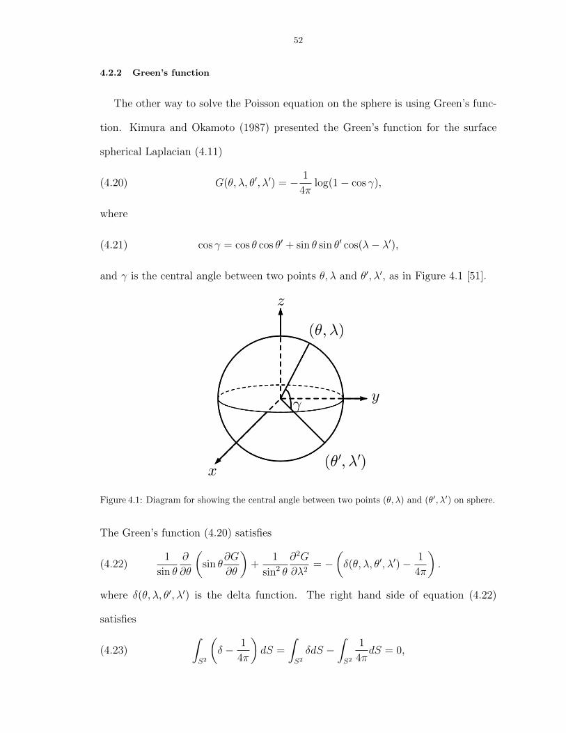
52

4.2.2 Green’s function

The other way to solve the Poisson equation on the sphere is using Green’s func-

tion. Kimura and Okamoto (1987) presented the Green’s function for the surface

spherical Laplacian (4.11)

(4.20) G(θ, λ, θ′, λ′) = − 1

4πlog(1− cos γ),

where

(4.21) cos γ = cos θ cos θ′ + sin θ sin θ′ cos(λ− λ′),

and γ is the central angle between two points θ, λ and θ′, λ′, as in Figure 4.1 [51].

(θ, λ)

(θ′, λ′)

γ

x

y

z


Figure 4.1: Diagram for showing the central angle between two points (θ, λ) and (θ′, λ′) on sphere.

The Green’s function (4.20) satisfies

(4.22)1

sin θ

∂

∂θ

(sin θ

∂G

∂θ

)+

1

sin2 θ

∂2G

∂λ2= −

(δ(θ, λ, θ′, λ′)− 1

4π

).

where δ(θ, λ, θ′, λ′) is the delta function. The right hand side of equation (4.22)

satisfies ∫S2

(δ − 1

4π

)dS =

∫S2

δdS −∫S2

1

4πdS = 0,(4.23)

53

which is a necessary condition for (4.9) to have a bounded solution on the sphere

[25], [18]. The formula (4.22) can be derived easily as we now show. Without loss of

generality, let’s suppose the source point θ′, λ′ is located at the north pole, that is,

θ′ = 0 and λ′ can be any real number, then by (4.21) we have cos γ = cos θ. Hence,

the Green’s function (4.20) depends on the colatitude θ only,

(4.24) G(θ) = − 1

4πlog(1− cos θ),

and the spherical Laplacian becomes,

(4.25) ∆s =1

sin θ

∂

∂θ

(sin θ

∂

∂θ

).

For θ > 0, that is, for all source points not at the north pole, we have

∆sG(θ) = − 1

4π

1

sin θ

∂

∂θ

(sin θ

∂G

∂θ

)(4.26)

= − 1

4π

1

sin θ

∂

∂θ

(sin2 θ

1− cos θ

)(4.27)

= − 1

4π

−(1− cos θ)2

(1− cos θ)2(4.28)

=1

4π.(4.29)

Next, we show that (4.22) holds in the sense of distribution.

Theorem IV.1. The Green’s function defined in (4.24) is a fundamental solution

of the Laplace equation on the sphere (4.11), that is, ∆sG = −δ+ 14π

in the sense of

distributions

(4.30) < ∆sG, f >=< −δ +1

4π, f >,

for any test function f(θ, λ).

54

Proof. The right hand side of (4.30) is

< −δ +1

4π, f > =

∫ 2π

0

∫ π

0

(−δ +1

4π)f(θ, λ) sin θdθdλ(4.31)

= −f(0, 0) +1

4π

∫ 2π

0

∫ π

0

f(θ, λ) sin θdθdλ.(4.32)

Since the Laplacian ∆s is a self-adjoint operator, we have

(4.33) < ∆sG, f >≡< G,∆sf >,

and

< G,∇2f > =

∫ 2π

0

∫ π

0

G1

sin θ

∂

∂θ

(sin θ

∂f

∂θ

)sin θdθdλ

+

∫ 2π

0

∫ π

0

G1

sin2 θ

∂2f

∂λ2sin θdθdλ.(4.34)

The second term in (4.34) is zero due to f is a periodic function on sphere, then we

have

(4.35) < G,∇2f >=

∫ 2π

0

∫ π

0

G1

sin θ

∂

∂θ

(sin θ

∂f

∂θ

)sin θdθdλ.

Plug in the Green’s function (4.24) to equation (4.35),

(4.36) < G,∇2f >= − 1

4π

∫ 2π

0

∫ π

0

log(1− cos θ)∂

∂θ

(sin θ

∂f

∂θ

)dθdλ

.

55

Then employ the integration by parts twice, we have

< G,∇2f > = − 1

4π

∫ 2π

0

log(1− cos θ) sin θ∂f

∂θ|πθ=0dλ−

∫ 2π

0

∫ π

0

sin θ∂f

∂θ

sin θ

1− cos θdθdλ

=

1

4π

∫ 2π

0

∫ π

0

∂f

∂θ

sin2 θ

1− cos θdθdλ

=1

4π

∫ 2π

0

f(θ, λ)sin2 θ

1− cos θ|πθ=0dλ−

∫ π

0

∫ 2π

0

f(θ)

(sin2 θ

1− cos θ

)′dθdλ

=1

4π

∫ 2π

0

f(θ, λ)1− cos2 θ

1− cos θ|πθ=0dλ+

∫ 2π

0

∫ π

0

f(θ, λ) sin θdθdλ

=

1

4π

∫ 2π

0

f(θ, λ)(1 + cos θ)|πθ=0dλ+

∫ 2π

0

∫ π

0


=

1

4π

∫ 2π

0

−2f(0, λ)dλ+

∫ 2π

0

∫ π

0


=

1

4π

−4πf(0, 0) +

∫ 2π

0

∫ π

0


= −f(0, 0) +

1

4π

∫ 2π

0

∫ π

0

f(θ, λ) sin θdθdλ.

For later reference, the Green’s function (4.20) can be written as

(4.37) G(x,x′) = − 1

4πlog(1− x · x′).

For points on the surface of a unit sphere, it is obvious that

(4.38) cos γ = x · x′,

which proves that (4.20) and (4.37) are equivalent. Using the Green’s function (4.20),

we can obtain the solution of Poisson equation (4.9),

(4.39) ψ(θ, φ) =1

4π

∫ ∫ζ(θ′, λ′) log(1− cos γ) sin θ′dθ′dλ′.

The relative vorticity ζ defined as a sum of δ functions,

(4.40) ζ(θ, λ) =N∑j=1

Γjδj(θ, λ, θj, λj),

56

where Γj is the strength of the jth point vortex at (θj, λj). This is the basic idea for

the point vortex method [51]. Next, we’ll introduce regularized point vortex method.

4.2.3 Regularized Green’s Function

The regularized point vortex model has been applied in vortex sheet simulation

and vortex dynamics on the sphere [52], [70]. It shows better properties than point

vortex model. The Green’s function given by (4.20) may be regularized as follows

(4.41) Gδ(θ, λ, θ′, λ′) = − 1

4πlog(1− cos γ + δ2),

where here δ > 0 is a small number. Now the question is what is the corresponding

vorticity field? Again, without loss of generality, we suppose the source point θ′, λ′ is

located at the north pole, then the Green’s function only depends on the colatitude

θ, that is,

(4.42) Gδ(θ) = − 1

4πlog(1− cos θ + δ2).

Taking the surface spherical Laplacian (4.11),

∆sGδ(θ) = − 1

4π

(1

sin θ

∂

∂θ

(sin θ

∂Gδ

∂θ

))(4.43)

= − 1

4π

(1

sin θ

∂

∂θ

(sin2 θ

1− cos θ + δ2

))(4.44)

= − 1

4π

(−(1− cos θ)2 + 2δ2 cos θ

(1− cos θ + δ2)2

)(4.45)

≈ −ζδ(θ).(4.46)

Figure 4.2 shows the regularized vorticity associated with the regularized Green’s

function Gδ(θ) for different δ. As we see from this Figure, as δ decreases, the vorticity

function tends to the spike delta function. This implies the regularized Green’s

function (4.42) is a good approximation of the Green’s function (4.20). For a source

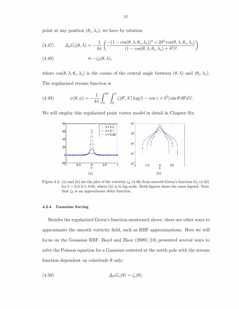
57

point at any position (θs, λs), we have by rotation

∆sGδ(θ, λ) = − 1

4π

(−(1− cos(θ, λ, θs, λs))2 + 2δ2 cos(θ, λ, θs, λs)

(1− cos(θ, λ, θs, λs) + δ2)2

)(4.47)

≈ −ζδ(θ, λ),(4.48)

where cos(θ, λ, θs, λs) is the cosine of the central angle between (θ, λ) and (θs, λs).

The regularized stream function is

(4.49) ψ(θ, φ) = − 1

4π

∫ 2π

0

∫ π

0

ζ(θ′, λ′) log(1− cos γ + δ2) sin θ′dθ′dλ′.

We will employ this regularized point vortex model in detail in Chapter Six.

(a) (b)

Figure 4.2: (a) and (b) are the plot of the vorticity ζδ (4.46) from smooth Green’s function Gδ (4.42)for δ = 0.2, 0.1, 0.05, where (b) is in log scale. Both figures share the same legend. Notethat ζδ is an approximate delta function.

4.2.4 Gaussian forcing

Besides the regularized Green’s function mentioned above, there are other ways to

approximate the smooth vorticity field, such as RBF approximations. Here we will

focus on the Gaussian RBF. Boyd and Zhou (2009) [18] presented several ways to

solve the Poisson equation for a Gaussian centered at the north pole with the stream

function dependent on colatitude θ only:

(4.50) ∆SGε(θ) = ζε(θ),

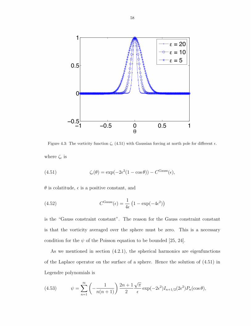
58

−1 −0.5 0 0.5 1−0.5

0

0.5

1

!

" = 20" = 10" = 5

Figure 4.3: The vorticity function ζε (4.51) with Gaussian forcing at north pole for different ε.

where ζε is

(4.51) ζε(θ) = exp(−2ε2(1− cos θ))− CGauss(ε),

θ is colatitude, ε is a positive constant, and

(4.52) CGauss(ε) =1

4ε

(1− exp(−4ε2)

)is the “Gauss constraint constant”. The reason for the Gauss constraint constant

is that the vorticity averaged over the sphere must be zero. This is a necessary

condition for the ψ of the Poisson equation to be bounded [25, 24].

As we mentioned in section (4.2.1), the spherical harmonics are eigenfunctions

of the Laplace operator on the surface of a sphere. Hence the solution of (4.51) in

Legendre polynomials is

(4.53) ψ =∞∑n=1

(− 1

n(n+ 1)

)2n+ 1

2

√π

εexp(−2ε2)In+1/2(2ε2)Pn(cos θ),

59

where the Pn(x) are the usual unnormalized Legendre polynomials and In+1/2 are the

usual modified spherical Bessel functions. The disadvantage of this solution formula

is that the rate of convergence of the series is slow for large ε, as shown in [18].

In [18] the exact solution formula for (4.51) is derived,

Gε(θ) =1

4ε2

1− exp(−4ε2)

log(1− µ)− 1

4ε2exp(−4ε2) log

(1 + µ

1− µ

)+

1

4ε2E1(2ε2[1− µ]) +

1

4ε2exp(−4ε2)Ei(2ε

2[1 + µ]),(4.54)

where µ = cos θ,

(4.55) E1(z) ≡∫ ∞

1

exp(−zt)

tdt,

and

(4.56) Ei(z) ≡ γ + log(z) +

∫ z

0

exp(t)− 1

tdt.

Note that the above solution (4.54) is a function of cos θ and ε only, and it can be

extended to the solution of Poisson equation with Gaussian at any position λs, θs by

rotation as we did in (4.47).

4.3 Rossby-Haurwitz Wave

4.3.1 Stream function

Note that an exact analytic solution of equation (4.9) can be obtained in the

special case where the stream function is equal to a single spherical harmonic. Thus

we let

(4.57) ψ(λ, µ, t) = ψm,n(t) exp(imλ)P nm(µ).

Substituting (4.57) into (4.12) and applying (4.15), we find that the non-linear advec-

tion terms are identically zero so that the amplitude coefficient satisfies the ordinary

60

Figure 4.4: Initial stream function with amplitude A = 0.05 and n = 1,m = 1.

linear differential equation

(4.58) −n(n+ 1)dψm,ndt

= −2Ωimψm,n,

which has the solution ψm,n(t) = ψm,n(0) exp(iνm,nt), where

(4.59) νm,n = 2Ωm/ [n(n+ 1)] ,

is the dispersion relation for the Rossby-Haurwitz wave [46].

4.3.2 Example

Here we take the simplest case as an example: n = 1,m = 1, then ν(m,n) = Ω.

The initial Rossby-Hauwritz wave is

(4.60) ψ(θ, λ) = A sin θ cosλ,

as in Figure 4.4 in spherical coordinates, where A is the amplitude of the wave. Its

61

Cartesian coordinate counterpart is

ψ = Ax,(4.61)

ζ = 2Ax.(4.62)

The stream function at time t is

ψ(θ, λ, t) = A sin θ cos(λ+ Ωt)(4.63)

= A sin θ (cosλ cos Ωt− sinλ sin Ωt)(4.64)

= A (x cos Ωt− y sin Ωt) .(4.65)

Figure 4.5 shows the stream lines at t = π, 2π, 3π, 4π with amplitude A = 0.05 and

angular velocity Ω = 1/2. We can see the wave propagates towards west with a

constant velocity Ω.

From (4.8) we have

u = (u, v, w)(4.66)

= ∇ψ × x(4.67)

= (∂ψ

∂yz − ∂ψ

∂zy)i + (

∂ψ

∂zx− ∂ψ

∂xz)j + (

∂ψ

∂xy − ∂ψ

∂yx)k(4.68)

that is,

u =∂ψ

∂yz − ∂ψ

∂zy,(4.69)

v =∂ψ

∂zx− ∂ψ

∂xz,(4.70)

w =∂ψ

∂xy − ∂ψ

∂yx.(4.71)

The trajectories of the fluid particles are obtained by solving the following set of

62

Figure 4.5: Stream function from equation (4.63) at t = π, 2π, 3π, 4π with amplitude A = 0.05 andangular velocity Ω = 1/2.

63

ODEs,

dx

dt= u = −Az sin Ωt,(4.72)

dy

dt= v = −Az cos Ωt,(4.73)

dz

dt= z = A(y cos Ωt+ x sin Ωt),(4.74)

Figure 4.6 shows the particle trajectories obtained by solving equations (4.72) to

(4.74) using fourth order Runge-Kutta for five revolutions, where A = 0.05 and

Ω = 1/2. We will compare these trajectories with numerical results obtained by the

RBF and point vortex methods described in the next two chapters.

(a) (b)Figure 4.6: Rossby-Haurwitz wave (n = m = 1). (a) : particle trajectories obtained by solving

equations (4.72) to (4.74) using fourth order Runge-Kutta for five revolutions, whereA = 0.05 and Ω = 1/2; (b): local zoom of the left figure.

In this chapter, we give an overview of the solutions of the barotropic vorticity

equation. It includes the spherical harmonic expansions, Green’s function on sphere

and Poisson equation with Gaussian forcing. The Rossby-Haurwitz wave example

will be tested by the numerical methods that we will employ in Chapters Five and

Six.

CHAPTER V

Solving the Barotropic Vorticity Equation by Gaussian RBF

5.1 Soving PDEs by RBF

The Radial Basis Function method has great potential not only for its ability

for scattered data interpolation in multi-dimensions but also for meshfree solving

PDEs. Kansa (1990) [49, 50] was the first person to solve PDEs by Multiquadric

RBF. His method consisted of approximating spatial partial derivatives by differen-

tiating smooth RBF interpolants to solve parabolic, elliptic, and viscously damped

hyperbolic PDEs to spectral accuracy in a completely mesh-free manner. Larsson

and Fornberg (2003) [54] proposed a method for solving elliptic PDEs by means of

collocation with both piecewise and infinitely smooth RBFs. They concluded that for

PDE applications with smooth solutions, the infinitely smooth RBFs are preferable

for higher accuracy. They also compared RBF-based methods against a second-order

finite difference method and a pseudospectral method and showed the former gave

a much superior accuracy. Flyer and Wright (2007) [32] solved hyperbolic partial

differential equations on a sphere. They showed that RBFs allow for a much lower

spatial resolution and are able to take unusually large time steps to achieve the same

accuracy as compared to other commonly used spectral methods on a sphere such as

spherical harmonics, double Fourier series, and spectral element methods. Flyer and

64

65

Wright (2009) [33] presented a radial basis function method for the shallow water

equations on a sphere. However all the existing approaches for solving PDE by RBFs

use an Eulerian formulation, that is, all the points that are the centers of the RBFs

are fixed in time. Here we present a way to solve the BVE by RBF in a Lagrangian

manner, which means, all the centers of RBFs are Lagrangian points which move

with the fluid flow.

5.2 Solving BVE by Gaussian RBF

The first step to solve the BVE by Gaussian RBF is to approximate the smooth

relative vorticity by Gaussians [8]. Let us expand the relative vorticity ζ by Gaussian

RBF (GARBF)

(5.1) ζ(θ, λ) =N∑j=1

dj(exp(−ε2r2

j )− CGauss(ε)),

where ε is an RBF parameter and rj is the Euclidean distance between the evaluation

points (θ, λ) and the centers (θj, λj),

(5.2) rj = r(θ, λ, θj, λj) =√

2(1− cos θ cos θj cos(λ− λj)− sin θ sin θj),

CGauss(ε) is the “Gauss constraint constant” defined in (4.52). The RBF coefficients

dj are obtained by interpolation as we mentioned in Chapter Two,

(5.3) s(θm, λm) =N∑j=1

dj(exp(−ε2r2

mj)− CGauss(ε))

= ζm,

where ζm = ζ(θm, λm) and rmj = r(θm, λm, θj, λj). Note that the basis functions

are Gaussians minus a constant since the total integral of the relative vorticity on

sphere should be zero, which is a necessary condition for Poisson equation (4.9) has a

bounded solution as we mentioned in Chapter Four. It is a slight difference compared

to the Gaussian RBF we defined in Chapter Two. Substituting (5.1) into the Poisson

66

equation (4.9), we have

(5.4) ∆sψ(θ, λ) = −ζ = −N∑j=1

dj(exp(−ε2r2

j )− CGauss(ε)).

Define ψj by

(5.5) ∆sψj(θ, λ) = exp(−ε2r2j )− CGauss(ε).

Since surface spherical Laplacian is a linear operator, then the stream function is

(5.6) ψ(θ, λ) = −∑j

djψj(θ, λ).

Boyd and Zhou (2009) presented the solution of the Poisson equation with Gaussian

forcing ψj in equation (4.54) [18] as introduced in Chapter Four, which is the solution

of equation (5.5). Then the stream function ψ(θ, λ) can be obtained by equation

(5.6). In order to get the velocity field, we need to know the gradient of the stream

function ψj, [18],

∂ψj∂λ

=∂ψj∂γ

∂γ

∂λ=∂ψj∂γ

(sin θj sin θ sin(λj − λ)) ,(5.7)

∂ψj∂θ

=∂ψj∂γ

∂γ

∂θ=∂ψj∂γ

(− cos θj sin θ + sin θj cos θ cos(λj − λ)) ,(5.8)

where

(5.9)∂ψj∂γ

=1

4ε2

(exp(−2ε2(1− γ))− 1

1− γ +exp(−2ε2(1− γ))− exp(1− 4ε2)

1 + γ

),

and γ is the central angle between (θ, λ) and (θj, λj) as defined in Figure 4.1. Now,

we have ODEs for the trajectory of the centers of the Gaussian RBFs,

dλmdt

=1√

1− µ2m

N∑j=1

dj sin θj sin θm sin(λj − λm)∂ψj∂γ|γ=γmj,(5.10)

dµmdt

=N∑j=1

dj(− cos θj sin θm + sin θj cos θm cos(λj − λm))∂ψj∂γ|γ=γmj,(5.11)

67

where µm = cos θm and γmj = cos θm cos θj+sin θm sin θj cos(λm−λj). We use fourth

order Runge-Kutta for time integration.

The description of the algorithm is as follows

• 1. Choose RBF initial centers, i.e., the initial distribution of points (θj, λj).

These points will move with the fluid flow and they are carrying vorticity. The

relative vorticity ζ is assigned to each point according to the initial vorticity

distribution. The absolute vorticity η can be calculated by ηj = ζj + 2Ω cos θj

and it is conserved due to equation (4.10).

• 2. Compute the RBF coefficients by interpolation as in (5.3). In this step, the

centers also play the role of interpolation points.

• 3. The points are evoluted by equations (5.10) and (5.11). The relative vorticity

is updated by ζj = ηj − 2Ω cos θj. If the current time is not the final time, go

to step 2.

Next we will show that GARBF method we used here is related to the point vortex

method. Note that Kimura and Okamoto (1987) [51] write the vorticity in terms of

the summation of Dirac delta function,

(5.12) ζ(θ, λ) =N∑j=1

Γjδ(θ, λ, θj, λj),

where Γj is the strength of the jth point vortex at (θj, λj). Substituting (5.12) into

(4.39), we have the velocity in the θ direction vθ and the λ direction vλ

vθ =1

sin θ

∂ψ

∂λ= − 1

4π

N∑j=1

Γjsin θj sin(λ− λj)

1− cos γ,(5.13)

vλ = −∂ψ∂θ

= − 1

4π

N∑j=1

Γjcos θ sin θj cos(λ− λj)− sin θ cos θj

1− cos γ,(5.14)

68

where γ is the central angle between point (θ, λ) and (θj, λj) as in Figure 4.1. Fur-

thermore, since a point vortex is advected by a velocity induced by other vortices,

the motion of the mth vortex is given by

θm =1

sin θ

∂ψ

∂λ= − 1

4π

N∑j=1,j 6=m

Γjsin θj sin(λm − λj)

1− cos γm,j,(5.15)

sin θmλm = −∂ψ∂θ

= − 1

4π

N∑j=1,j 6=m

Γjcos θm sin θj cos(λm − λj)− sin θm cos θj

1− cos γm,j.(5.16)

Note that the equation system (5.10) and (5.11) from GARBF are very similar to the

one (5.15) and (5.16) from point vortex method. Note that the former one converges

to the later one as the Gaussians become infinitely narrow, that is, ε goes to infinity.

This idea of interpolation the vorticity is from Beale. Next we will present several

numerical experiments using the ODE system (5.10) and (5.11).

5.3 Rossby-Haurwitz Wave

As mentioned in Chapter Four, a Rossby-Haurwitz wave is an exact solution of

the BVE. Here we use the same example as in section (4.3.2): n = 1,m = 1, νmn = Ω.

The initial stream function is the same as in (4.65), the relative vorticity at time t is

(5.17) ζ(θ, λ, t) = 2A sin θ cos(λ+ Ωt),

by which we can test our numerical results. Next we choose Sadourney’s icosahedral

points [69] as RBF centers where we expand the relative vorticity. We leave the

detailed discussion of the point generation to Chapter Six, where we will discuss

other choices of the point distribution on the sphere in detail. Figure 5.1 is the

illustration of N = 20 and N = 80 icosahedral points on a sphere. The absolute

error is defined,

(5.18) EAbs(θ, λ, t) = |ζex(θ, λ, t)− ζRBF (θ, λ, t)|,

69

where ζex is the exact relative vorticity given by (5.17) and ζRBF is the numerical

result calculated by (5.1). The error is evaluated at longitude-latitudinal grid. The

relative error is defined,

(5.19) Erela(θ, λ, t) =|ζex(θ, λ, t)− ζRBF (θ, λ, t)|∞

|ζex(θ, λ, t)|∞.

We analyze the temporal and spatial convergence of the numerical result in the

following sections.

(a) (b)Figure 5.1: Illustration of icosahedral points on the surface of the sphere with (a) n = 20 and (b)

n = 80.

We can also do a rigorous error analysis since we have the exact solution of

the PDE. The parameters that control the accuracy of the method include spatial

discretization N , time step ∆t and RBF parameter ε. Figure 5.2 is the absolute error

of GARBF defined in equation (5.18) after one revolution with N = 20, ∆t = 4π/200

and ε = 0.1. It is impressive since there are only 20 points on sphere. Figure 5.3

shows the relative error defined by (5.19) of the vorticity obtained by GARBF after

one revolution (t = 4π) when the number of timesteps is 25, 50, 100, 200, 400. The

total number of points is 20 and ε = 0.1. We see that the relative error decreases at

the rate O((∆t)4), which agrees with our expectation of fourth-order Runge-Kutta.

On the other hand, we can see that the relative error is around 10−8 even though

70

we only use n = 20 points on the sphere. Figure 5.4 shows the relative error and

the condition number of the RBF matrix A (see equation (2.7)) versus the RBF

parameter ε. We can see that as ε decreases, the relative error first decreases, then

increases. The reason is that for small ε, the condition number of the interpolation

matrix A is large and the interpolation system is ill-conditioned. This introduces

error even though theoretically the RBF method has high accuracy when ε is small

[37].

Figure 5.2: Absolute error of vorticity defined by (5.18) which is obtained by GARBF after onerevolution (t = 4π) with N = 20, ∆t = 4π/200, ε = 0.1.

10−2 10−1 10010−10

10−5

100

! t

rela−errO(! t)4

Figure 5.3: Relative error defined by (5.19) of vorticity obtained by GARBF after one revolution(t = 4π) for the number of timesteps is 25, 50, 100, 200, 400. Total number of points is20 and ε = 0.1.

71

0.4 0.6 0.8 110−8

10−7

10−6

10−5

!

rela−err

(a)

0.4 0.6 0.8 1106

108

1010

1012

1014

!

cond(A)

(b)Figure 5.4: (a): The relative error defined by (5.19) of vorticity obtained by GARBF with ∆t =

4π/200, n = 80 for different ε; (b): the condition number of RBF matrix A.

5.4 One Vortex Patch

Our next numreical experiment is the evolution of a Gaussian vortex. For a fixed

Gaussian shape parameter β, let the initial vorticity be

(5.20) ζ(λ, θ) = exp(−2β2(1− cos(λ, θ, λc, θc)))− CGauss,

where (λc, θc) is the center of the vortex and the Gaussian, β controls the shape of

the Gaussian, here and in the following sections, we fix λc = π/3, θ = π/3 and β = 4.

CGauss is the Gauss constraint as we mentioned in chapter 4,

(5.21) CGaussian =1− exp(−4β2)

4β2,

and cos(λ, θ, λc, θc) is the cosine of the angle between point (λ, θ) and (λc, θc) as in

(4.21)

5.4.1 Choosing RBF parameter ε

For RBF approximation, the numerical error is not only related to the timestep

and spatial discretization, but also highly depends on the parameter ε. As we dis-

cussed in Chapter Two, there is a tradeoff in choosing ε. Large ε will give an inaccu-

rate approximation. However, a small ε leads to an ill-conditioned RBF interpolation

matrix, which will damage the accuracy of the approximation too. We choose our ε

72

by checking the accuracy of the initial vorticity interpolation. Suppose we have an

RBF approximation for the above initial vorticity

(5.22) ζRBF(λ, θ) =N∑j=1

dj exp(−ε2r(θ, λ, θj, λj)2),

where θj, λj, j = 1 : N are N interpolation points (we call them nodes later) and

r(θ, λ, θj, λj) is the Euclidean distance between (θ, λ) and (θj, λj). We choose ε by

experiments. Since the initial vorticity is highly concentrated around the region that

is close to the center of the Gaussian, we put more nodes around this area, as in

Figure 5.5. We define the relative error at t = 0 for RBF approximation:

(5.23) E2 =|ζEX − ζRBF|∞|ζEX|∞

.

Table 5.1 shows the RBF approximation for fixed points n = 170 as in Figure 5.5

with different ε, which is uniform for all points. Again, it shows the tradeoff of the

choice of ε. Small ε means better accuracy but worsens the condition number of

interpolation matrix. Note that

(5.24) α = εhmin,

is the relative width parameter, where hmin is the minimum distance between any

two points.

For the nonuniform grid distribution, Fornberg and Zuev (2009) [38] show that a

spatially variable shape parameter ε has a better performance than uniform ε. They

took

(5.25) εj =1

dj,min

,

where dj,min is the Euclidean distance between the node (λj, θj) and its closest neigh-

bor node. Figure 5.6 shows the absolute error for the relative vorticity with fixed

ε = 6 and variable ε as defined in (5.25) for points in Figure 5.5.

73

Figure 5.5: Interpolation points for initial vorticity; refined spherical triangular mesh (which will bediscussed in detail in Chapter Six); number of points is 170, minimum distance betweentwo points are 0.0451.

ε α E2 cond(A)

4 0.1804 0.0071 2.8158e+015

5 0.2255 0.0123 7.3093e+012

6 0.2706 0.0149 6.0551e+010

7 0.3158 0.0157 1.2360e+009

8 0.3609 0.0159 5.1877e+007

Table 5.1: Relative Error for RBF approximation on a sphere with fixed number of interpolationpoints and different ε (uniform). α is defined in equation (5.24).

In a more recent paper, Flyer and Lehto [31] present the other choice of ε for

nonuniform points on sphere,

(5.26) εj = εmin

(maxjdj,min

dj,min

),

and εmin O(1) is a scaling parameter. We experiment the above ε choice by choosing

different εmin and find that for the εmin which makes the absolute error of the initial

relative vorticity acceptable, the condition number is large. Figure 5.7 shows the

absolute error of the relative vorticity and Table 5.2 is the condition number. We

74

(a) (b)

Figure 5.6: Absolute error of relative vorticity computed in grid in Figure 5.5. (a): fixed ε; (b):ε adoptive from (5.25). Note that the maximum error occurs where the mesh changesfrom coarse to fine.

see that varying the ε value using the formula given in (5.25) still has the trade-off

between accuracy and ill-conditioning.

εmin cond(A)

1 6.1871e+012

0.8 1.9754e+016

0.6 2.6365e+019

0.4 3.4059e+019

Table 5.2: Condition number for εmin = 1, 0.8, 0.6, 0.4.

We conducted similar experiments for ε in (5.25) and found the same problem.

We did the tests for time integration and had even worse results. Since the choice of

the ε is so important for RBF methods, this will be the subject of our future work.

5.5 Two Vortex Patches on a Non-rotating Sphere

Vortex patch interaction is an interesting topic in fluid dynamics. Levy, Nair and

Tufo (2009) [56] and Shin [71] experimented that the vortex patch interaction on a

β−plane. Here we suppose there are two disk-shaped vortex patches on the surface

of the sphere. For a non-rotating sphere, when the diameter of the disk is much less

75

(a) (b)

(c) (d)

Figure 5.7: Absolute error of relative vorticity for different εmin. Note that the maximum erroroccurs where the mesh changes from coarse to fine.

than the radius of the earth, we can approximate the surface of the sphere by a plane

with a free boundary.

5.5.1 Initial patches

Now we explain how to get the disk-shaped patch on sphere. We first get points

which form the patch on the plane then project them to the surface of the sphere by

azimuthal projection

(5.27) xs =x

|x| .

All the points are the centers of a hexagon. The center of the circular disk is one

of the points that we need. The variable nNIHS controls the number of points at

half side, as in Figure 5.8. For example, in Figure 5.8 (a), nNIHS equals two, that

means, there are two points on the left side of the center of the circle. In Figure 5.8

76

(b), (c) and (d), the value of nNIHS equals 4, 8 and 16 respectively. By this way,

the distance of each particle to its neighbors is the same.

(a) (b)

(c) (d)

Figure 5.8: Points in a disk on a plane. The nNIHS = 2,4,8,16. Every point is at the center of ahexagon.

5.5.2 Numerical integration

In this test, we suppose two patches carry equal positive vorticities. They have

same number of points N = 1459. The distance between the two centers is r = 2.6.

Figure 5.9 shows how two vortex patches interact with each other at t = 0, t = 2, t =

3. The reason for different color of the two patches is to distinguish them. The shape

of the patches agrees with the figures shown in the work of Waugh [75].

The two patch interaction test here is only limited to the non-rotating sphere. The

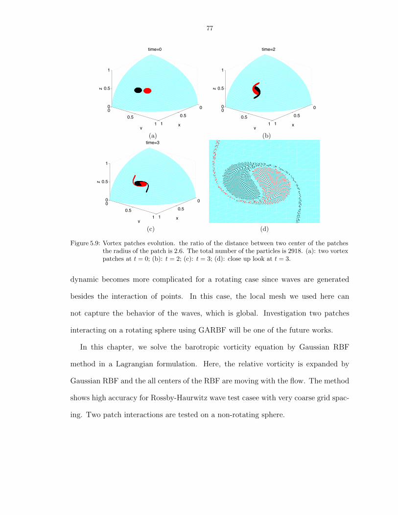
77

00.5

1

00.5

1

0

0.5

1

x

time=0

y

z

(a)

00.5

1

00.5

1

0

0.5

1

x

time=2

y

z

(b)

00.5

1

00.5

1

0

0.5

1

x

time=3

y

z

(c) (d)

Figure 5.9: Vortex patches evolution. the ratio of the distance between two center of the patchesthe radius of the patch is 2.6. The total number of the particles is 2918. (a): two vortexpatches at t = 0; (b): t = 2; (c): t = 3; (d): close up look at t = 3.

dynamic becomes more complicated for a rotating case since waves are generated

besides the interaction of points. In this case, the local mesh we used here can

not capture the behavior of the waves, which is global. Investigation two patches

interacting on a rotating sphere using GARBF will be one of the future works.

In this chapter, we solve the barotropic vorticity equation by Gaussian RBF

method in a Lagrangian formulation. Here, the relative vorticity is expanded by

Gaussian RBF and the all centers of the RBF are moving with the flow. The method

shows high accuracy for Rossby-Haurwitz wave test casee with very coarse grid spac-

ing. Two patch interactions are tested on a non-rotating sphere.

CHAPTER VI

Solving the Barotropic Vorticity Equation by VortexMethod

6.1 Introduction

The vortex method is characterized by both considering the PDE in stream

function-vorticity form and Lagrangian discretization of the vorticity. There is a

variety of literature in this field [9, 21, 23, 52, 55, 68]. For problems on the sur-

face of the earth, the application of vortex method is an active area. Zabusky and

McWilliams (1982) presented a modulated point vortex model for BVE and com-

pared the results with a finite difference model on the beta plane approximation

[78]. Yao, Zabusky and Dritschel [77] compared contour surgery with pseudospectral

simulations. Newton and Shokraneh (2006) investigated the dynamics of N-point

vortices on a rotating unit sphere [63]. Newton and Sakajo (2007) studied the evolu-

tion of N-point vortices in a ring formation embedded in a background flow field that

initially corresponds to solid-body rotation on a sphere. The evolution of the point

vortices is tracked numerically as an embedded dynamical system along with the M

contours which separate strips of constant vorticity [64]. Sakajo (2004) considered

the motion of a vortex sheet on the surface of a unit sphere in the presence of point

vortices fixed on north and south poles [70]. Sakajo (2009) presented a fast algorithm

for two vortex sheets rolling-up on the surface of the sphere.

78

79

6.2 Lagrangian Fomulation of BVE

First, let us invert the Poisson equation (4.9) by expressing the stream function

as a convolution of the Green’s function (4.37) and the vorticity [51],

(6.1) ψ(x, t) = − 1

4π

∫S2

log(1− x · x′)ζ(x′, t)dS(x′).

Applying Equation (6.1) to Equation (4.9) yields the velocity,

(6.2) u(x, t) = − 1

4π

∫S2

x× x′

1− x× x′ζ(x′, t)dS(x′).

Given the velocity field u(x, t), we define the flow map x(a, t) by the equation

(6.3)∂x

∂t(a, t) = u(x(a, t)),

where a is a set of Lagrangian parameters on the sphere. We assume that

(6.4) x(a, 0) = a,

so the flow map at t = 0 is the identity on the sphere. Equation (6.2) and (6.3) then

yield

(6.5)∂x

∂t(a, t) = − 1

4π

∫S2

x(a, t)× x′

1− x(a, t) · x′ ζ(x′, t)dS(x′).

The next step is to change variables using the flow map, x′ = x(a′, t), which yields

(6.6)∂x

∂t(a, t) = − 1

4π

∫S2

x(a, t)× x(a′, t)

1− x(a, t) · x(a′, t)dΓ(a′, t),

where the circulation element is defined by

(6.7) dΓ(a′, t) = ζ(x(a′; t), t)dS(x(a′; t)).

The goal is to discretize the evolution equation for the flow map (6.6). We dis-

cretize the surface of the earth by panels (spherical triangular or quadrilateral). The

80

panels evolve in time under the action of the flow map, and their shape changes, but

they retain their identity in Lagrangian parameter space. Each panel has a particle

at its center and we obtain an equation of motion for the particles by discretizing

Equation (6.5) for the flow map using midpoint rule. The result is a set of ODEs for

the motion of the particles,

(6.8)dxjdt

= − 1

4π

N∑k=1,k 6=j

xj × xk1− xj · xk

ζkAk,

where ζk is the relative vorticity at kth panel and Ak is the area of the panel, which

is a triangle or quadrilateral. We will discuss the area formula later. Note that

k 6= j means we skip the singular panels. Now, introduce two sets of points, active

points and passive points. Active points are at the center of the panels and carry

vorticitiy. The relative vorticity of kth panel is the same as the relative vorticity at

kth active point. Passive points are at the vertices of the panels and advected by

active points. Figure 6.1 shows active points and the passive points for both triangle

and quadrilateral panels. The absolute vorticity is conserved for each active point

(4.10), that is, ηk = ηk0, where ηk0 denotes kth active point’s initial absolute vorticity.

With the help of the relation between absolute vorticity and relative vorticity ηk =

ζk + 2Ωzk, we have

(6.9) ζk + 2Ωzk = ζk0 + 2Ωzk0,

then,

(6.10) ζk = ζk0 + 2Ωzk0 − 2Ωzk,

where ζk0 + 2Ωzk0 is the absolute vorticity of kth active point at t = 0. Next, we will

discuss the meshes on the surface of a sphere.

81

(a) (b)

Figure 6.1: Active points (•) and passive points () of a triangle and quadrilateral panel.

6.3 Meshes on the Surface of the Sphere

We need to discretize the flow map equation (6.6) on sphere. The first question is:

what is the mesh? Here we investigate four different types of meshes on the surface of

the sphere: Longitude-Latitude (LL), Icosahedral Triangle (IT), Icosahedral Hexagon

(IH) and Cubed Sphere (CS).

6.3.1 Longitude-latitude (LL)

The longitude-latitude mesh is the most nature mesh for the spherical geometry.

However, we can see from Figure 6.2 that the mesh introduces the polar singularity,

that is, all the meridian lines converge to points on both the south and the north

poles. Points are clustered around the poles, on the other hand, equatorial resolution

is much poorer.

(a) (b)

Figure 6.2: Longitude-Latitude Panel. (a): side view; (b): view from north pole. Points areclustered at the pole area.

82

6.3.2 Icosahedral triangles (IT)

First we project the 12 vertices of an icosahedron to a unit sphere. The Cartesian

coordinates define the vertices of an icosahedron with edge-length 2, centered at the

origin:

(0,±1,±gr), (±1,±gr, 0), (±1, 0,±gr)

where gr = (1 +√

5)/2 is the golden ratio. For the IT mesh and the following icosa-

hedral hexagon and cubed-sphere mesh, we will use a parameter L which controls the

level of global refinement and the total number of panels N . We call the projection

points of 12 vertices of the icosahedron the vertices of icosahedral triangles. The first

level L = 0 of the IT mesh is obtained by connecting the vertices with their closest

points using great circles, as in the first graph in Figure 6.4 [69, 76]. The center c of

the triangle is obtained by averaging 3 vertices vi, i = 1, 2, 3,

(6.11) c =v1 + v2 + v3

3,

where v1, v2, v3 are the Cartesian coordinates of three vertices, then projecting c to

the unit sphere

(6.12) c =c

|c| .

This mesh can be nested refined by connecting the center of each edge by great

circles as shown in Figure 6.3. For example, v12 is the center of the edge v1v2. The

coordinate of the new center c1 is the average of three vertices vc, v12, v31 by equation

(6.11) then project to the sphere by equation (6.12). Figure 6.4 and Figure 6.5 shows

the global and local refinement. The red and the yellow colors indicate some local

features that we want to resolve and where local mesh refinement is needed. Figure

83

6.6 shows the ratio of the minimum area of maximum area for each global refinement,

the mesh becomes more uniform as the number of points increases.

v1 v2

v3

c

v12

v23v31

c1


Figure 6.3: Icosahedral triangle mesh refinement stencils. For example, new vertices v12 is thecenter of the edge v1v2. The coordinate of the new center c1 is the average of threevertices v1, v12, v31 by equation (6.11) then project to the sphere by equation (6.12).

L = 0 L = 1 L = 2 L = 3

Figure 6.4: Icosahedral triangles. From left to right: L = 0, 1, 2, 3 and n = 20, 80, 320, 1280. Ver-tices are projections from 12 vertices of an icosahedron to a unit sphere.

Figure 6.5: Icosahedral triangles with local refinement. The red and yellow colors indicate somelocal features that we want to resolve and where local mesh refinement is needed.

6.3.3 Icosahedral hexagon (IH)

The icosahedral hexagon is a dual mesh for icosahedral triangle mesh, as in Figure

6.7. It is also called spherical geodesic mesh in [67]. The IH mesh is built upon IT

mesh in the following way. Suppose we created the icosahedral triangle mesh, then

84

100 1050.75

0.8

0.85

0.9

0.95

1area ratio

number of points

Figure 6.6: The ratio of minimum area and maximum area in Icosahedral triangle mesh. This showsthe mesh becomes more uniform as the number of points increases.

connect the centers of each neighbor panel, where neighbor means that the panels

share the same edge, that forms the IH panels. The difficulty with this icosahedral

hexagon mesh is that it is hard to implement nested refinement. We can refine the

hexagon to triangles by connecting the centers and the vertices of the hexagon as an

alternative way. This is the subject of future work.

L = 0 L = 1 L = 2 L = 3

Figure 6.7: Icosahedral hexagon. From left to right: L = 0, 1, 2, 3 and n = 12, 42, 162, 642. Thevertices of the hexagon/pendagon are the centers of the spherical triangle in figure (6.4).

6.3.4 Cubed-sphere (CS)

The last spherical grid which we shall consider here is the cubed-sphere mesh.

Figure 6.8 shows a circumscribed cube in a sphere, where eight vertices of the cube

are on the sphere. The cubed-sphere mesh is defined by a radial projection from

the center of the cube inscribed into the sphere (a so-called “gnomonic projection”).

There are various versions of the cubed-sphere mesh. First we will explain the method

85

in [65] and then the approach that implemented in this thesis.

Figure 6.8: a circumscribed cube in a sphere

6.3.4.1 gnomonic projection

A local Cartesian coordinate system is determined for each of the six faces of the

cube. Suppose the local coordinates are (x, y)i, which rang from [−a, a] for cube faces

i ∈ 1 : 6 where a =√

33

for unit sphere. Then the spherical coordinates (X, Y, Z) for

the local face centered in the −Y is

(6.13) (X, Y, Z) =1

r(x,−a, y), r =

√a2 + x2 + y2,

By this way, each point on the cube is connected to a point on the spherical surface.

6.3.4.2 chord projection

In numerical tests in this thesis, we use a different way to generate the cubed-

sphere mesh. Let us start with eight vertices of a circumscribed cube as in Figure 6.8.

The first level of panels is obtained by connecting the vertices which share the same

side by great circles. Figure 6.9 shows the refinement stencils of the cubed-sphere

mesh. For example, new vertices v12 is the center of the edge v1v2. The coordinate

of the new center c1 is the average of three vertices v1, v12, vc, v41 by equation (6.11)

then project to the sphere by equation (6.12), where vc is at the same position as the

86

center c. Figure 6.10 is the global refined cubed-sphere mesh with n = 6, 24, 96, 384.

Figure 6.11 shows local refinement of the cubed-sphere mesh, where the red and

yellow colors indicate some local features that we want to resolve and where local

mesh refinement is needed.

v1 v2

v4 v3

c

v12

vc v23

v34

v41

c1


Figure 6.9: Cubed-sphere mesh refinement stencils. For example, new vertices v12 is the centerof the edge v1v2. The coordinate of the new center c1 is the average of four verticesv1, v12, vc, v41 by equation (6.11) then project to the sphere by equation (6.12), wherevc is at the same position as the center c.

L = 0 L = 1 L = 2 L = 3

Figure 6.10: Cubed-sphere mesh with n = 6, 24, 96, 384. The first eight vertices of quadrilateralpanels are the vertices of a circumscribed cube.

Figure 6.11: Cubed-sphere local refinement. The red and yellow colors indicate some local featuresthat we want to resolve and where local mesh refinement is needed.

In this chapter, the numerical tests are performed in both icosahedral triangle

mesh and cubed-sphere mesh. Next, we will talk about the area of the panels on the

surface of the sphere.

87

6.4 Area for Panels on Sphere

As we mentioned before, the midpoint method is applied in evaluating the Biot-

Savart integral (6.5). Then we need a way to calculate the area for panels on sphere in

equation (6.8). The Cartesian coordinates of the vertices of each panel are available.

Let A, B and C be row vectors which contain the Cartesian coordinates of the

vertices of a spherical triangle as shown in Figure 6.12, that is, A = (xA, yA, zA),

B = (xB, yB, zB), C = (xC , yC , zC). α, β, γ are angles of spherical triangle. The sides

of the triangle a, b and c are part of great circles. Since A,B,C are unit vectors, we

have

cos a = B · C;(6.14)

cos b = A · C;(6.15)

cos c = A ·B;(6.16)

We suppose a, b, c are less than π so we take arccos directly. The formula for the

spherical excess E is presented in ([1]) (Pg. 468-469),

(6.17) tanE

4=

√tan

s

2tan

s− a2

tans− b

2tan

s− c2

,

where s = (a+ b+ c)/2. There is a relation between the spherical excess E and the

area of a spherical triangle ([1])

(6.18) Area = R2E,

where R is the radius of the sphere (R = 1 in our case). That is the way that we

obtain the area of the panel from the Cartesian coordinates of the vertices of the

panel.

Four panels have other shapes, we first decompose them to triangles then sum the

area of triangles. For example, the area of the quadrilateral is computed by treating

88

Figure 6.12: Angles of the spherical triangles.

the quadrilateral as two spherical triangles and applying the formula (6.18) twice.

In our numerical tests, the spherical triangular area formula (6.18) will be applied in

equation (6.8). Next, we will discuss the regularized approximation of the Green’s

function that we applied in the numerical experiments.

6.5 Regularized Approximation

As we discussed in Chapter Four, the point vortex methods approximate the

vorticity by the Dirac delta function. The vortex blob method has more advantages

since the basis functions have more overlap. Here we use a regularized Green’s

function (4.41) as we introduced in Chapter Four, the stream function ψδ

(6.19) ψδ(x, t) = − 1

4π

∫S2

log(1− x · x′ + δ2)ζ(x′, t)dS(x′),

where δ > 0 is a small number. Discretization on the surface of the sphere leads to

(6.20) ψδ(xi, t) = − 1

4π

N∑j=1

log(1− xi · xj + δ2)ζ(xj, t)Aj,

89

where xj and Aj are the center and the area of the jth panel. The ODE system for

the flow map becomes

(6.21)dxjdt

= − 1

4π

N∑k=1,k 6=j

xj × xk1− xj · xk + δ2

ζkAk.

For future referece, the approximate vorticity is

−ζδ(θ, λ) = ∆sψδ(θ, λ)

(6.22)

= ∆s

(− 1

4π

∫ 2π

0

∫ π

0

log(1− cos(θ, λ, θ′, λ′) + δ2)ζ(θ′, λ′)dθ′dλ′)

= − 1

4π

(∫ 2π

0

∫ π

0

∆s log(1− cos(θ, λ, θ′, λ′) + δ2)ζ(θ′, λ′)dθ′dλ′)

= − 1

4π

(∫ 2π

0

∫ π

0

(−(1− cos(θ, λ, θ′, λ′))2 + 2δ2 cos(θ, λ, θ′, λ′)

(1− cos(θ, λ, θ′, λ′) + δ2)2

)ζ(θ′, λ′)dθ′dλ′

)≈ − 1

4π

∑j

((−(1− cos(θ, λ, θj, λj))2 + 2δ2 cos(θ, λ, θj, λj)

(1− cos(θ, λ, θj, λj) + δ2)2

)ζjAj

),

where ζj = ζ(θj, λj) and Aj is the area of the jth panel. The relative vorticity at

any point of the sphere can be calculated by equation (6.22). This formula is useful

when we apply the remeshing strategy, which we will discuss later.

Next, we start the numerical experiments. The first one is the Rossby-Haurwitz

wave.

6.6 Rossby-Haurwitz Wave Experiments

As we mentioned in Chapter Four, the Rossby Haurwitz (RH) wave is an exact

solution for the BVE. It is a reasonable first test case for our numerical method. Here

and in the following subsections, we focus on the simplest case as in Chapter Four,

that is m = 1, n = 1 and amplitude A = 0.05 RH wave. Without loss of generality,

we fix Ω = 1/2, then t = 4π represents one revolution. Fourth-order Runge-Kutta is

used for time integration.

90

6.6.1 Definition of error

Since the Rossby-Haurwitz wave is the exact solution of the BVE, we can inves-

tigate the errors. For the stream function ψ, let us the define relative error

(6.23) RelaErr =||ψex − ψδ||∞||ψex||∞

.

For the position of particles, we suppose Pi = (Pxi, Pyi, Pzi) and Pei = (Pexi, P eyi, P ezi)

as our numerical position and exact position at time t for point i. Let

(6.24) AbsErr = maxi||Pi − Pei||∞

be our error criteria.

6.6.2 Mesh comparison

We apply three different meshes: icosahedral triangle, icosahedral hexagon and

cubed-sphere to calculate the evolution of the RH wave. Figure 6.13 shows the

absolute error for the particle position after one revolution. The error is comparable

for the three meshes. Then we will focus on the icosahedral triangle mesh for the

remaining Rossy-Haurwitz wave tests.

6.6.3 Timestep experiments

Table 6.1 and 6.2 show the absolute error defined in (6.24) for fixed number of

points N = 320, N = 1280 respectively. We can see that the error converges to a

saturation error which is due to the spatial discretization. For the later experiments

with the RH wave, we fix ∆t = 4π/1600. Figure 6.14 shows the fourth-order con-

vergence in time for the difference between absolute error and the saturation error,

where we choose the error from ∆t = 4π/3200 as the saturation error.

91

101 102 103 10410−4

10−3

10−2

10−1Position Error, 1 rev.

number of points

Abso

lute

Erro

r in

posit

ion AbsErrHex

O(1/n)AbsErrCubeAbsErrTri

Figure 6.13: Absolute error in particle positions after one revolution for different meshes: icosa-hedral triangle, icosahedral hexagon and cubed-sphere for RH wave. The error iscomparable for the three meshes. All three lines are parallel to the line O(1/n), whichmeans the vortex method we use here is first order accurate in terms of the number ofpoints.

6.6.4 Test spatial error

Table 6.3 shows the absolute error defined in (6.24) for the fixed timestep ∆t =

4π/1600. Figure 6.15 shows that the numerical method is first order accurate in the

number of the panels on sphere.

Figure 6.16 is the trajectory of particles after five revolutions with N = 80,∆t =

4π/1600, which is agree to the one we obtained from exact ODE equations (4.72) to

(4.74) and Figure 4.6.

6.6.5 Stream function

The initial stream function is given by (4.61). We first solve the stream function

given by (6.1) using the midpoint numerical integral based on spherical triangle (IT)

mesh, then compare it with the exact one (4.61). Figure 6.17 shows that the relative

error (6.23) is almost proportional to the area of the spherical triangular panel, which

agrees with the fact that the midpoint rule is a second-order method. Figure 6.18

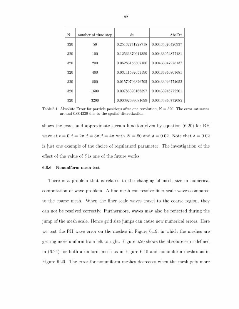
92

N number of time step dt AbsErr

320 50 0.25132741228718 0.00434076420937

320 100 0.12566370614359 0.00433954877181

320 200 0.06283185307180 0.00433947278137

320 400 0.03141592653590 0.00433946803681

320 800 0.01570796326795 0.00433946774052

320 1600 0.00785398163397 0.00433946772201

320 3200 0.00392699081699 0.00433946772085

Table 6.1: Absolute Error for particle positions after one revolution, N = 320. The error saturatesaround 0.004339 due to the spatial discretization.

shows the exact and approximate stream function given by equation (6.20) for RH

wave at t = 0, t = 2π, t = 3π, t = 4π with N = 80 and δ = 0.02. Note that δ = 0.02

is just one example of the choice of regularized parameter. The investigation of the

effect of the value of δ is one of the future works.

6.6.6 Nonuniform mesh test

There is a problem that is related to the changing of mesh size in numerical

computation of wave problem. A fine mesh can resolve finer scale waves compared

to the coarse mesh. When the finer scale waves travel to the coarse region, they

can not be resolved correctly. Furthermore, waves may also be reflected during the

jump of the mesh scale. Hence grid size jumps can cause new numerical errors. Here

we test the RH wave error on the meshes in Figure 6.19, in which the meshes are

getting more uniform from left to right. Figure 6.20 shows the absolute error defined

in (6.24) for both a uniform mesh as in Figure 6.10 and nonuniform meshes as in

Figure 6.20. The error for nonuniform meshes decreases when the mesh gets more

93

N number of time step dt AbsErr

1280 50 0.25132741228718 0.00124543628511

1280 100 0.12566370614359 0.00124419067101

1280 200 0.06283185307180 0.00124411317947

1280 400 0.03141592653590 0.00124410835356

1280 800 0.01570796326795 0.00124410805258

1280 1600 0.00785398163397 0.00124410803379

1280 3200 0.00392699081699 0.00124410803262

Table 6.2: Absolute error for particle positions after one revolution, N = 1280. The error saturatearound 0.001244 due to the spacial discretization.

N AbsErr

20 0.05602181188586

80 0.01549499404301

320 0.00433946772201

1280 0.00124410803379

Table 6.3: Absolute error for particle position after one revolution with fixed ∆t = 0.00785 inicosahedral triangular mesh for different spacial resolution N = 20, 80, 320, 1280.

uniform. Define

(6.25) ratio =AbsErrCR

AbsErrC

,

where AbsErrCR denotes the absolute error calculated on a cubed-sphere refined

mesh in Figure 6.19 and AbsErrC denotes the absolute error calculatd on a uniform

cubed-sphere mesh in figure 6.10. Figure 6.20 (b) shows the ratio of the error defined

in (6.25). When the ratio less then one, it means that the nonuniform mesh has larger

error than the uniform mesh. However, we also see that the nonuniform mesh has

smaller errors when N = 456 and N = 1572, which means that the non-uniformity

of the mesh does not cause severe problem in our method.

94

10−3 10−2 10−1 10010−15

10−10

10−5

100

dt

||Abs

olut

e Er

ror −

Sat

urat

ion

Erro

r||

AbsErr n=320AbsErr n=1280O(dt4)

Figure 6.14: Plot |AbsErr−SaturationError| versus dt, which shows the 4th order accuracy of RK4with N = 320, 1280. star: N = 320 ; circle: N = 1280 .

Here, we finish the numerical tests for the Rossby-Haurwitz wave. Now we will

focus on problems that don’t have an analytical solution, but based around physical

phenomenon [56]: vortex patch evolution. Before we start the numerical experiments,

we first discuss the adaptive mesh refinement strategy that we will apply.

6.7 Adaptive Mesh Refinement (AMR)

For computational fluid dynamics, adaptive local mesh refinement is an attractive

strategy since it offers better spatial resolution for resolving small scale features and

does not require a fine mesh for the whole computational domain [13, 14, 47, 48].

Here we will discuss the AMR for vortex method [30] and focus on local refinement

for the icosahedral triangle and the cubed-sphere mesh. We use two refinement

criteria εΓ and εd. When the circulation of the panel is larger than εΓ or the panel’s

side length is larger than εd, the panel is divided into four smaller ones as shown

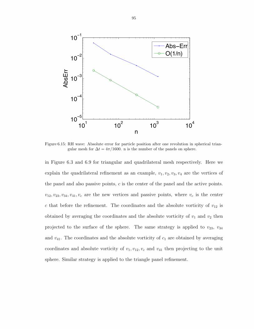
95

101 102 103 10410−5

10−4

10−3

10−2

10−1

n

AbsErr

Abs−ErrO(1/n)

Figure 6.15: RH wave: Absolute error for particle position after one revolution in spherical trian-gular mesh for ∆t = 4π/1600. n is the number of the panels on sphere.

in Figure 6.3 and 6.9 for triangular and quadrilateral mesh respectively. Here we

explain the quadrilateral refinement as an example, v1, v2, v3, v4 are the vertices of

the panel and also passive points, c is the center of the panel and the active points.

v12, v23, v34, v41, vc are the new vertices and passive points, where vc is the center

c that before the refinement. The coordinates and the absolute vorticity of v12 is

obtained by averaging the coordinates and the absolute vorticity of v1 and v2 then

projected to the surface of the sphere. The same strategy is applied to v23, v34

and v41. The coordinates and the absolute vorticity of c1 are obtained by averaging

coordinates and absolute vorticity of v1, v12, vc and v41 then projecting to the unit

sphere. Similar strategy is applied to the triangle panel refinement.

96

Figure 6.16: Trajectory of particles after five revolutions with N = 80, dt = 4π/1600, which is agreeto the one we obtained from exact ODE equations (4.72) to (4.74) and figure (4.6).

6.8 Gaussian Vortex Tests

Suppose the initial vorticity is a Gaussian centered at xc = (xc, yc, zc)

(6.26) ζ(x,xc) = exp(−2ε2(1− x · xc))− CGauss,

where ε controls the width of the Gaussian. We fix ε = 4 in the following sections.

CGauss is the Gauss constraint ([18]), which is a constant that only depends on ε,

(6.27) CGaussian =1− exp(−4ε2)

4ε2,

which guarantees that the total vorticity over the surface of the sphere is zero. Since

the initial vorticity is highly non-uniform, local adaptive mesh refinement is neces-

sary. Here we employ three user-specified parameters L, εΓ, εd to control the mesh.

The goal is to have a relatively fine mesh at the place where small-scale events de-

velop. We start with a uniform mesh with L levels. L should not be too small or too

large. Large L means heavy computational cost, however, if L is too small, it can not

catch the features of the Gaussian. Parameter εΓ is criterion for the circulation of the

panel. Recall the procedure for panel refinement was explained in section 6.3, Figure

6.9 and Figure 6.3. The panel is refined to several smaller ones if the circulation

is larger than εΓ. As time goes on, the panels are stretched by the flow and if the

97

10−4 10−2 10010−5

100rela err

area

rela−errO(area)

Figure 6.17: Relative error (6.23) of the stream function (6.1) using midpoint numerical integralbased on spherical triangle (ST). Area means the maximum area of the sphericaltriangle since they are not exactly the same.)

length of any side is larger than εd, the panel is refined. The investigation of other

refinement criterion is the subject of future work. Table 6.4 shows the parameters

we use for the test cases involving the Gaussian patch. First we test the non-rotating

sphere then the rotating one.

6.8.1 Non-rotating sphere

When the background sphere is not rotating, that is, Ω = 0, the Gaussian patch

is self-rotating. Figure 6.21 shows the test case 1 in table 6.4. The center of the

patch is at (0, 1, 0). We can see from the number of panels N that under the same

refinement criteria, there is more refinement for the icosahedral triangle mesh than

for the cubed-sphere mesh. The patch preserves the symmetric shape as time goes

on. We also observe the artificial diffusion in this test case, which is due to the linear

interpolation we used here for adaptive refinement. High order interpolation scheme

98

(a) (b)

(c) (d)

Figure 6.18: Exact and approximate (6.20) stream function for RH wave at t = 0, t = 2π, t =3π, t = 4π with n = 80 and δ = 0.02

will be employed in the future.

6.8.2 Rotating sphere

Figure 6.22 shows the evolution of the Gaussian patch at t = 0, t = 2π, t = 4π for

cubed-sphere and icosahedral triangle mesh respectively with Ω = 1/2, L = 4, εΓ =

0.0002, εd = 0.02 (test case 2 in table 6.4). In both cubed-sphere and icosahedral tri-

angle mesh, the Gaussian patch moves to the northwest direction due to the Coriolis

force, which is agree to our expectation [56].

6.8.3 Convergence check

We test the Gaussian patch on a rotating sphere Ω = 1/2 after one revolution

t = 4π by systematically changing the refinement criterion εΓ, leaving L and εd

fixed. Figure 6.23 shows the Gaussian vortex patch after one revolution with fixed

99

N = 120 N = 180 N = 456 N = 1572


Figure 6.19: Meshes for N = 120, 180, 456, 1572 for testing the effect of mesh non-uniformity.

(a) (b)

Figure 6.20: (a): absolute error for particle positions for uniform cubed-sphere mesh as in figure(6.10) and nonuniform cubed-sphere meshes as in figure (6.19); Right : ratio of twoabsolute errors defined in (6.25).

L = 4, εd = 0.02 and εΓ = 0.001, 0.0005, 0.0002, 0.0001. It shows that the shape of

the patch converges to a similar pattern. More rigorous convergence check will be

done in the future.

6.9 Two Gaussian Vortices Test

Suppose now we initially have two Gaussian patches centered at (xc1, yc1, zc1) =

(−0.3670, 0.8548, 0.3670) and (xc2, yc2, zc2) = (0.3670, 0.8548, 0.3670).

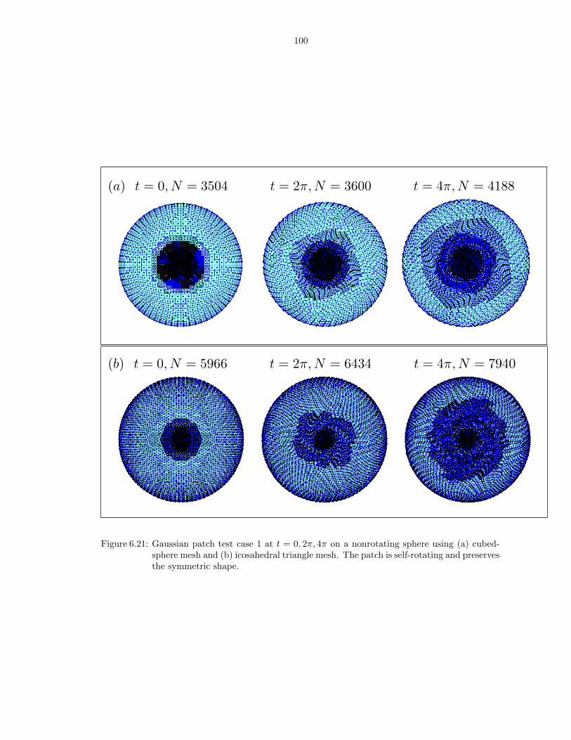
100

(a) t = 0, N = 3504 t = 2π,N = 3600 t = 4π,N = 4188


(b) t = 0, N = 5966 t = 2π,N = 6434 t = 4π,N = 7940


Figure 6.21: Gaussian patch test case 1 at t = 0, 2π, 4π on a nonrotating sphere using (a) cubed-sphere mesh and (b) icosahedral triangle mesh. The patch is self-rotating and preservesthe symmetric shape.

101

(a) t = 0, N = 3504 t = 2π,N = 3594 t = 4π,N = 3993


(b) t = 0, N = 5966 t = 2π,N = 6347 t = 4π,N = 7799


Figure 6.22: Gaussian patch test case 2 at t = 0, 2π, 4π on a rotating sphere. (a): cubed-spheremesh; (b) icosahedral triangle mesh. Gaussian patch moves in the northwest directionwhich agrees with the physical expectation.

N = 2856 N = 3102 N = 3993 N = 6306


Figure 6.23: Gaussian patch test case 3. From left to right, εΓ = 0.001, 0.0005, 0.0002, 0.0001 att = 4π. We can observe qualitative convergence property.

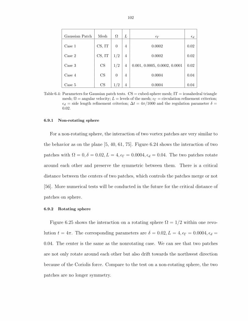
102

Gaussian Patch Mesh Ω L εΓ εd

Case 1 CS, IT 0 4 0.0002 0.02

Case 2 CS, IT 1/2 4 0.0002 0.02

Case 3 CS 1/2 4 0.001, 0.0005, 0.0002, 0.0001 0.02

Case 4 CS 0 4 0.0004 0.04

Case 5 CS 1/2 4 0.0004 0.04

Table 6.4: Parameters for Gaussian patch tests. CS = cubed-sphere mesh; IT = icosahedral trianglemesh; Ω = angular velocity; L = levels of the mesh; εΓ = circulation refinement criterion;εd = side length refinement criterion; ∆t = 4π/1000 and the regulation parameter δ =0.02.

6.9.1 Non-rotating sphere

For a non-rotating sphere, the interaction of two vortex patches are very similar to

the behavior as on the plane [5, 40, 61, 75]. Figure 6.24 shows the interaction of two

patches with Ω = 0, δ = 0.02, L = 4, εΓ = 0.0004, εd = 0.04. The two patches rotate

around each other and preserve the symmetric between them. There is a critical

distance between the centers of two patches, which controls the patches merge or not

[56]. More numerical tests will be conducted in the future for the critical distance of

patches on sphere.

6.9.2 Rotating sphere

Figure 6.25 shows the interaction on a rotating sphere Ω = 1/2 within one revo-

lution t = 4π. The corresponding parameters are δ = 0.02, L = 4, εΓ = 0.0004, εd =

0.04. The center is the same as the nonrotating case. We can see that two patches

are not only rotate around each other but also drift towards the northwest direction

because of the Coriolis force. Compare to the test on a non-rotating sphere, the two

patches are no longer symmetry.

103

t = 0, N = 3444 t = 2π,N = 3450 t = 4π,N = 3573


Figure 6.24: Gaussian patch test case 4 at t = 0, π, 3π on a nonrotating sphere. The initial centers oftwo patches are (−0.3670, 0.8548, 0.3670) and (0.3670, 0.8548, 0.3670). The two patchesrotate around each other and merge.

t = 0, N = 3444 t = 2π,N = 3444 t = 3π,N = 3543


Figure 6.25: Gaussian patch test case 5 at t = 0, π, 3π on a rotating sphere. The initial centers oftwo patches are (−0.3670, 0.8548, 0.3670) and (0.3670, 0.8548, 0.3670). The two patchesrotate around each other and merge and both are drift towards the northwest direction.

104

6.10 Remeshing

From the test cases for the Gaussian patches for example as in Figure 6.21, we

can see that the panel meshes are no longer regular after a long time integration.

Remeshing is one of the ideas to restore a regular mesh and preserve the accuracy of

computation. Since the initial mesh is constructed by initial vorticity distribution, we

reconstruct the current mesh using the current vorticity distribution. The question

is: we know the vorticity that each active point carries, how to calculate it at a

regular mesh point? First we choose the number of levels L, then calculate ζ at each

center of the new panels by (6.22) for a specified parameter δ. The ζj in equation

(6.22) is the relative vorticity that carries by active points. Then repeat the meshing

procedure we employed at t = 0. We conduct remeshing at t = 2π and t = 4π

for Gaussian patch on a non-rotating sphere. Figure 6.26 shows two preliminary

results of remeshing with δ = 0.025. In this figure, the panels in (a) and (c) before

the remeshing are severely deformed. They are no longer regular quadrilaterals in

physical space. From (b) and (d), we can see that the remeshing is doing is good

job since it captures the vorticity and also preserves some symmetry of the vorticity

field. Developing accurate and efficient remeshing strategy is the subject of our

future work.

6.11 Comparison of Vortex Method with GARBF Method

In Chapters five and six, we presented two methods for solving the Barotropic

Vorticity Equation. They are both Lagrangian methods since all the grid points are

moving with the flow and they both utilize a fourth-order Runge Kutta method in

time. Here we present a brief comparison.

• Accuracy/Convergence. The vortex method is first order accurate in terms of

105

before after(a)


(b)


(c)


(d)



Figure 6.26: Preliminary results of remeshing. Retain the relative vorticity at L = 4 uniform meshwith δ = 0.02 using equation (6.22) then refined with εΓ = 0.0004 and εd = 0.02. (a)and (c) are the Gaussian patch test at t = 2π and t = 4π with Ω = 0, L = 4, εΓ = 0.0004and εd = 0.02,∆t = 4π/1000, δ = 0.02; (b) and (d) are the meshs after remeshing for(a) and (c) respectively.

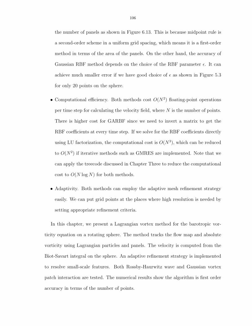
106

the number of panels as shown in Figure 6.13. This is because midpoint rule is

a second-order scheme in a uniform grid spacing, which means it is a first-order

method in terms of the area of the panels. On the other hand, the accuracy of

Gaussian RBF method depends on the choice of the RBF parameter ε. It can

achieve much smaller error if we have good choice of ε as shown in Figure 5.3

for only 20 points on the sphere.

• Computational efficiency. Both methods cost O(N2) floating-point operations

per time step for calculating the velocity field, where N is the number of points.

There is higher cost for GARBF since we need to invert a matrix to get the

RBF coefficients at every time step. If we solve for the RBF coefficients directly

using LU factorization, the computational cost is O(N3), which can be reduced

to O(N2) if iterative methods such as GMRES are implemented. Note that we

can apply the treecode discussed in Chapter Three to reduce the computational

cost to O(N logN) for both methods.

• Adaptivity. Both methods can employ the adaptive mesh refinement strategy

easily. We can put grid points at the places where high resolution is needed by

setting appropriate refinement criteria.

In this chapter, we present a Lagrangian vortex method for the barotropic vor-

ticity equation on a rotating sphere. The method tracks the flow map and absolute

vorticity using Lagrangian particles and panels. The velocity is computed from the

Biot-Savart integral on the sphere. An adaptive refinement strategy is implemented

to resolve small-scale features. Both Rossby-Haurwitz wave and Gaussian vortex

patch interaction are tested. The numerical results show the algorithm is first order

accuracy in terms of the number of points.

CHAPTER VII

Summary and Future work

7.1 Thesis Summary

In Chapter One we introduce the motivation and the outline of the thesis. Chapter

Two gives an introduction to the RBF method, including its background, advantage

and related problems. The most significant property of RBF approximation is the

trade-off between exponential convergence and ill-conditioning. We also present an

RBF cardinal function for Gaussian in one dimensional unbounded evenly spaced

grid. At the end of this chapter, we compare the accuracy of RBF and finite dif-

ferences in terms of Fourier analysis of the eigen-function exp(iKX). One of the

major concerns of the applications of RBF is the computational cost. Chapter three

presents a fast treecode algorithm for evaluating RBFs. Instead of using direct sum-

mation between each pair of points, it applies a divide-and-conquer strategy to use

particle- cluster interactions. Taylor approximation is applied for the far-field ex-

pansion. The treecode reduces the computational cost from O(N2) to O(N logN),

where N is the number of particles in the system. The following three chapters are

applications related to the fluid flow on the surface of the sphere. Chapter four in-

troduces the Barotropic Vorticity Equation(BVE), which is the simplest atmospheric

model. Chapters five and six solve BVE by Gaussian RBF and vortex methods in

107

108

Lagrangian form. The Rossby-Haurwitz wave and Gaussian patch are tested in both

chapters.

7.2 Improving the Vortex/RBF Method for solving BVE

We will keep improving the vortex/RBF method for solving BVE in the following

aspects.

• ε for nonuniform grid on sphere. ε is important for solving PDEs by RBF method

accurately. For nonuniform grid, ε needs to vary according to the grid size. We

did experiments for two ε choices reported in the literature [31], [38]. They both

don’t work well since ill-conditioning is still an issue. Hence, looking for a better

choice of ε is a task for future work.

• Remeshing. Remeshing is an important step to preserve the accuracy of the

computation. There are two major points that we need to consider. The first

is the experiments of choosing a reasonable value of δ. The second one is the

efficiency of the remeshing step.

• Check energy conservation. Energy conservation a very important property for

a numerical algorithm. The vortex method conserves circulation, which is a

very good property.

• High order mesh refinement strategy. Our current strategy for local mesh re-

finement is using linear interpolation to find the position of the new points. We

may apply high order interpolation to increase the accuracy. Figure 7.1 shows

a way to have quadratic interpolation. For example, each cubic panel has eight

passive points and one active point in Figure 7.1(a). There are three points on

each side, then quadratic interpolation can be applied to calculate the position

109

of new points.

(a) (b)

Figure 7.1: Stencils for high order refinement. (a): one active point and eight passive points inquadrilateral panel; (b): one active point and 6 passive points in triangular panel.

7.3 Shallow Water Equation (SWE)

The SWEs are an ideal testbed for numerical method in geophysical fluid flow.

The equations are

∂u

∂t+ u · ∇u + f × u = −g∇h(7.1)

∂h

∂t+ u · ∇h+ h∇ · u = 0,(7.2)

where u is the horizontal velocity, h is the layer height, f = fkandf = 2Ω cos θ is

the Coriolis parameter [74, 72]. The velocity can be recovered from vorticity and

divergence by solving

∆ψ = ζ,(7.3)

∆χ = δ,(7.4)

u = k ×∇ψ +∇χ(7.5)

[72]. We can do this by a strategy similar to that for the barotropic vorticity equa-

tion, which uses Green’s function in vortex method and the solution of the Poisson

equation with Gaussian forcing in Gaussian RBF.

7.4 Application and Extension of Treecode

In our current application projects, both Gaussian RBF and Vortex methods

are O(N2) system, where N is the number of points. A treecode can reduce the

110

t = 0 t = 15

t = 20 t = 20


Figure 7.2: Vortex sheet evolution t = 0, 15, 20 and the last one is a close-up at t = 20.

computational cost to O(N logN). Our current treecode works for particles in three

dimension. It works for particles both in a cube and on a surface of the sphere. Since

we are interested in geophysical problems, which are on the spherical geometry, we

will tailor the treecode to fit our simulation. For example, instead of using cubic box

as our clusters, we can use spherical triangles as an alternative. We believe it will

be more efficient since we will be using the quad-tree structure on a two dimension

manifold instead of an oct-tree structure in space.

7.5 Jet Simulation

A vortex sheet is a material surface in the fluid across which the tangential com-

ponent of fluid velocity has a jump discontinuity [29]. They are frequently used as

an asymptotic model for parallel shear flow. It can also be applied to jet simulation,

which is a very common phenomenon in atmosphere. Figure 7.2 is a vortex sheet

roll-up on the sphere at t = 0, 15, 20. This shows we can do jet simulation using two

vortex sheets with opposite sign. The other way to simulate jet is using barotropic

vorticity equation, where the initial vorticity is two rings which are parallel to the

latitude circle.

BIBLIOGRAPHY

111

112

BIBLIOGRAPHY

[1] CRC Standard Mathematical Tables and Formulae. CRC Press, 1996.

[2] M. Abramowitz and I.A. Stegun. Handbook of Mathematical Functions. Dover, New York,1965.

[3] J. Adem. A series solution for the barotropic vorticity equation and its application in the studyof atmospheric vortices. Tellus, 3:364–372, 1956.

[4] A. Arakawa and V.R. Lamb. Computational Design of the Basic Dynamical Processes of theUCLA General Circulation Model. San Francisco: Academic Press, 1977.

[5] L. A. Barba and A. Leonard. Emergence and evolution of tripole vortices from net-circulationinitial conditions. Phys. Flui, 19.

[6] J.E. Barnes. A modified tree code: Don’t laugh; it runs. J. Comput. Phys., 87:161–170, 1990.

[7] J.E. Barnes and P. Hut. A hierarchical O(N logN) force-calculation algorithm. Nature,324(4):446–449, 1986.

[8] J.T. Beale. On the accuracy of vortex methods at large times. Springer-Verlag, New York,1988.

[9] J.T. Beale and A. Majda. Vortex methods I: Convergence in three dimensions. Math. Comput.,29(159):1–27, 1982.

[10] R.K. Beatson and L. Greengard. A Short Course on Fast Multipole Method. Oxford UniversityPress, 1997.

[11] R.K. Beatson and G.N. Newsam. Fast evaluation of radial basis functions: I. Comput. Math.Applic., 24(12):7–19, 1992.

[12] R. Bellman. A Brief Introduction to Theta Functions. Holt, Rinehart and Winston, New York,1961.

[13] M. J. Berger and P. Colella. Local adaptive mesh refinement for shock hydrodynamics. J.Comput. Phys., 82:64–84, 1989.

[14] M. J. Berger and J. Oliger. Adaptive mesh refinement for hyperbolic partial differential equa-tions. J. Comput. Phys., 53:484–512, 1984.

[15] J.P. Boyd. Chebyshev and Fourier Spectral Methods. Dover, 1990.

[16] J.P. Boyd and L. Wang. An analytic approximation to the cardinal functions of Gaussianradial basis functions on an infinite lattice. Appl. Math. Compu., 215:2215–2223, 2009.

[17] J.P. Boyd and L. Wang. Truncated gaussian RBF differences are always inferior to finitedifferences of the same stencil width. Commu. Comput. Phys., 5:42–60, 2009.

113

[18] J.P. Boyd and C. Zhou. Three ways to solve the possion equation on a sphere with Gaussianforcing. J. of Comput. Phys., 228:4702–4713, 2009.

[19] M.D. Buhmann. Radial Basis Functions: Theory and Implementations, Cambridge Mono-graphs on Applied and Computational Mathematics. Cambridge University Press, 2003.

[20] J.G. Charney, R. Fjortoft, and J.G. von Neumann. Numerical integration of the barotropicvorticity equation. Tellus, 2:237–254, 1950.

[21] H. Chen and J.S. Marshall. A Lagrangian vorticity method for two-phase particulate flowswith two-way phase coupling. J. Comput. Phys., 148.

[22] J.B. Cherrie, R.K. Beatson, and G.N. Newsam. Fast evaluation of radial basis function methodsfor generalized multiquadrics in Rn. SIAM J. Sci. Comput, 23(5):1549–1571, 2002.

[23] A.J. Chorin and P.S. Bernard. Discretization of a vortex sheet. J. Comput. Phys., 13:423–429,1973.

[24] D.G. Crowdy. Gaussian vortices on a sphere. private communication.

[25] D.G. Crowdy. Stuart vortices on a sphere. J.Fluid Mech., 498:381–402, 2004.

[26] M. DeMaria. Tropical cyclone motion in a nondivergent barotropic model. Mon. Wea. Rev.,113:1199–1210, 1985.

[27] J. Duchon. Splines minimizing rotation invariant seminorms in sobolev spaces. constructivetheory of functions of several variables, 1:85–100, 1976.

[28] K.G. Evans, D.W. Rouson, A.G. Salinger, M.A. Taylor, W. Weijer, and J.B. White. A Scalableand Adaptable Solution Framework within Components of the Community Climate SystemModel. Springer-Verlag Berlin, Heidelberg, 2009.

[29] H. Feng. Vortex Sheet Simulations of 3D Flows Using an Adaptive Triangular Panel/ParticleMethod. PhD thesis, University of Michigan, Ann Arbor, 2007.

[30] H. Feng, L. Kaganovskiy, and R. Krasny. Azimuthal instability of a vortex ring computed bya vortex sheet panel method. Fluid Dyn. Res., 41:051405, 2009.

[31] N. Flyer and E. Lehto. Rotational transport on a sphere: Local node refinement with radialbasis functions. J. Comput. Phys., 229:1954–1969, 2009.

[32] N. Flyer and G. Wright. Transport schemes on a sphere using radial basis functions. J.Comput. Phys., 229:1954–1969, 2007.

[33] N. Flyer and G. Wright. A radial basis function method for the shallow water equations on asphere. Proc. R. Soc. A, 465:1949–1976, 2009.

[34] B. Fornberg and N. Flyer. Accuracy of radial basis function interpolation and derivativeapproximations on 1-d infinite grids. Adv. Comput. Math., 23:5–20, 2005.

[35] B. Fornberg, N. Flyer, S. Hovde, and C. Piret. Localization properties of rbf expansion coeffi-cients for cardinal interpolation. i. equispaced nodes. Adv. Comput. Math., 47:5–20, 2006.

[36] B. Fornberg and C. Piret. A stable algorithm for flat radial basis functions on a sphere. SIAMJ. Sci. Comp., 30:60–80, 2007.

[37] B. Fornberg and G. Wright. Stable computation of multiquadric interpolants for all values ofthe shape parameter. Comp. Math. Appl., 48:853–867, 2004.

[38] B. Fornberg and J. Zuev. The runge phenomenon and spatially variable shape parameters inRBF interpolation. Adv. Comput. Math., 47:5–20, 2006.

114

[39] R. Franke. Scattered data interpolation: Tests of some methods. Math. Comp., 38:181–200,1982.

[40] O.U. Velasco Fuentes. Vortex filamentation: its onset and its role on axisymmetrization andmerger. Dyna. Atmo. Ocea., 40:23–42, 2005.

[41] I.S. Gradshteyn and I.M. Ryzhik. Table of Integrals, Series, and Products, fourth ed. AcademicPress, 1965.

[42] L. Greengard. The numerical solution of the N-body problem. Comput. Phys., pages 142–152,1990.

[43] L. Greengard and V. Rokhlin. A fast algorithm for particle simulations. J. Comput. Phys.,73:325–348, 1987.

[44] L. Greengard and J. Strain. The fast gauss transform. SIAM J. Sci. Stat. Comput., 12(1):79–94, 1991.

[45] R.L. Hardy. Multiquadric equations of topography and other irregular surfaces. J. Geophy.Res., 76:1905–1915, 1971.

[46] J.R. Holton. An Introduction to Dynamic Meteorology. Elsevier, 2004.

[47] C. Jablonowski. Adaptive Grids in Weather and Climate Modeling. PhD thesis, University ofMichigan, 2004.

[48] C. Jablonowski, M. Herzog, J. E. Penner, R. C. Oehmke, Q. F. Stout, B. van Leer, and K. G.Powell. Block-structured adaptive grids on the sphere: Advection experiments. Mon. Wea.Rev., 134:3691–3713, 2006.

[49] E.J. Kansa. Multiquadrics - a scattered data approximation scheme with applications to com-putational fluid-dynamics. i. surface approximations and partial derivative estimates. Comput.Math. Appl., 19:127–145, 1990.

[50] E.J. Kansa. Radial basis function for the sphere. Comput. Math. Appl., 19:147–161, 1990.

[51] Y. Kimura and H. Okamoto. Vortex motion on a sphere. J. Phys. Soc. Japan, 56(12):4203–4206, 1987.

[52] R. Krasny. Desingularization of periodic vortex sheet roll-up. J. Comput. Phys., 65(2):292–313,1986.

[53] R. Krasny and L. Wang. A treecode for fast summation of multiquadric RBFs. SIAM J. Sci.Compu., submitted.

[54] E. Larsson and B. Fornberg. A numerical study of some radial basis function based solutionmethods for elliptic PDEs. Comput. Math. with Appl., 46(6):891–902, 2003.

[55] A. Leonard. Vortex methods for flow simulation. J. Comput. Phys., 37:289–335, 1980.

[56] M.M. Levy, R.D. Nair, and H.M. Tufo. A high-order element-based Galerkin method for thebarotropic vorticity equation. Int. J. Numer. Meth. Fluids, 59:1369–1387, 2009.

[57] P. Li, H. Johnston, and R Krasny. A Cartesian treecode for screened coulomb interactions. J.Comput. Phys., 228:3858–3868, 2009.

[58] K. Lindsay and R. Krasny. A particle method and adaptive treecode for vortex sheet mothionin three-dimensional flow. J. Comput. Phys., 172:879–907, 2001.

[59] O.E. Livne and G.B. Wright. Fast multilevel evaluation of smooth radial basis function ex-pansions. ETNA, 23:263–287, 2006.

115

[60] J.B. Lundberg and B.E. Schutz. Recursion formulas of Legendre functions for use with non-singular geopotential models. J. Guid., Contr., and Dynam. (ISSN 0731-5090), 11:31–38,1988.

[61] P. Meunier, U. Ehrenstein, T. Leweke, and M. Rossi. A merging criterion for two-dimensionalco-rotating vortices. Phys. Fluid, 14(8).

[62] C.A. Micchelli. Interpolation of scattered data: Distance matrices and conditionally positivedefinite finctions. Constr. Approx., 2:11–22, 1986.

[63] P. K. Newton and H. Shokraneh. The n-vortex problem on a rotating sphere: I. multi-frequencyconfigurations. Proc. R. Soc., 462:149–169, 2006.

[64] P.K. Newton and T. Sakajo. The n-vortex problem on a rotating sphere: III. ring configurationcoupled to a background filed. Proc. R. Soc., 463:961–977, 2007.

[65] W.M. Putman and S.J. Lin. Finite-volume transport on various cubed-sphere grids. J. Com-put. Phys., 227:55–78, 2007.

[66] D.A. Randall. General Circulation Model Development: Past, Present and Future. AcademicPress, 2000.

[67] T.D. Ringler and D.A. Randall. A potential enstrophy and energy conserving numerical schemefor solution of the shallow-water equations on a geodesic grid. Mon. Wea. Rev., 130(5):1397–1410, 2002.

[68] G. Russo and J.A. Strain. Fast triangulated vortex methods for the 2D Euler equation. J.Comput. Phys., 111:291–323, 1994.

[69] R. Sadourny, A. Arakawa, and Y. Mintz. Integration of the nondivergent barotropic vorticityequation with an icosahedral-hexagonal grid for the sphere. Mon. Wea. Rev., pages 351–355,1968.

[70] T. Sakajo. Motion of vortex sheet on a sphere with pole vortices. Phys. Fluids, 16(3):717–727,2004.

[71] S.E. Shin, J.Y. Han, and J.J. Baik. On the critical separation distance of binary vortices in anondivergent barotropic atmoshphere. J. Meteo. Soc. Japan, 84:853–869, 2006.

[72] R.K. Smith and D.G. Dritschel. Revisiting the Rossby-Haurwitz wave test case with contouradvection. J. Comput. Phys., 217:473–484, 2006.

[73] M.J. Stock. Summary of vortex methods literature. http://markjstock.org/research.

[74] G. K. Vallis. Atmospheric and Oceanic Fluid Dynamics. Cambridge University Press, 2006.

[75] D.W. Waugh. The efficiency of symmetric vortex merger. Phys. Fluids A, 4(8):1745–1758,1992.

[76] D.L. Williamson. Integration of the barotropic vorticity equation on a spherical geodesic grid.Tellus, 20(4):642–653, 1968.

[77] H.B. Yao, N.J. Zabusky, and D.G. Dritschel. High gradient phenomena in two-dimensionalvortex interactions. Phys. Fluids, 7(3), 1993.

[78] N.J. Zabusky and J.C. McWilliams. A modulated point-vortex model for geostrophic, β-planedynamics. Phys. Fluid, 25(12):2175–2182, 1982.

Documents

Radial Basis Functions and Vortex Methods and their - Deep Blue