Radiance Interpolants for Interactive Scene Editingand Ray Tracing

by

Kavita Bala

September 1999

c©Massachusetts Institute of Technology 1999

This report is a minor revision of the dissertation of the same title submit-ted to the Department of Electrical Engineering and Computer Science onSeptember 10, 1999, in partial fulfillment of the requirements for the degreeof Doctor of Philosophy in that department. The thesis was supervised byProfessor Julie Dorsey and Professor Seth Teller.

This work was supported by an Alfred P. Sloan Research Fellowship (BR-3659), an NSF CISE Research Infrastructure award (EIA-9802220), anONR MURI Award (SA-15242582386), and a grant from Intel Corporation.

Massachusetts Institute of TechnologyLaboratory for Computer ScienceCambridge, Massachusetts, USA

Radiance Interpolants for Interactive Scene Editing

and Ray Tracingby

Kavita Bala

Abstract

Ray tracers are usually regarded as off-line rendering algorithms that are too slow for interactive

use. This thesis introduces techniques to accelerate ray tracing and to support interactive editing of

ray-traced scenes. These techniques should be useful in many applications, such as architectural

walk-throughs, modeling, and games, and will enhance both interactive and batch rendering.

This thesis introduces radiance interpolants: radiance samples that can be used to rapidly

approximate radiance with bounded approximation error. Radiance interpolants capture object-

space, ray-space, image-space and temporal coherence in the radiance function. New algorithms

are presented that efficiently, accurately and conservatively bound approximation error.

The interpolant ray traceris a novel renderer that uses radiance interpolants to accelerate both

primary operations of a ray tracer: shading and visibility determination. Shading is accelerated by

quadrilinearly interpolating the radiance samples associated with a radiance interpolant. Determi-

nation of the visible object at each pixel is accelerated by reprojectinginterpolants as the user’s

viewpoint changes. A fast scan-line algorithm then achieves high performance without sacrificing

image quality. For a smoothly varying viewpoint, the combination of lazily sampled interpolants

and reprojection substantially accelerates the ray tracer. Additionally, an efficient cache manage-

ment algorithm keeps the memory footprint of the system small with negligible overhead.

The interpolant ray tracer is the first accelerated ray tracer that reconstructs radiance from

sparse samples while bounding error conservatively. The system controls error by adaptively sam-

pling at discontinuities and radiance non-linearities. Because the error introduced by interpolation

does not exceed a user-specified bound, the user can trade performance for quality.

The interpolant ray tracer also supports interactive scene editing with incrementalrendering; it

is the first incremental ray tracer to support both object manipulation and changes to the viewpoint.

A new hierarchical data structure, called the ray segment tree, tracks the dependencies of radiance

interpolants on regions of world space. When the scene is edited, affected interpolants are rapidly

identified and updated by traversing these ray segment trees.

Keywords: 4D interpolation, error bounds, interactive, interval arithmetic, radiance approxi-

mation, rendering, visibility

3

Acknowledgments

There are many people I should thank for supporting me through my Ph.D. First, I would like to

thank my advisors, Prof. Seth Teller and Prof. Julie Dorsey, who gave me a chance; I entered the

field of graphics four years ago with no prior experience, and they took me on and were patient as

I learned the ropes. Working with them has been a wonderful learning experience; I have benefited

greatly from their knowledge of the field. They have taught me how to articulate my ideas and

how to step back to see the bigger picture and to aim high. I particularly appreciate the freedom

they gave me to explore my ideas; while this freedom has taken me down some garden paths, it

has taught me a lot about the research process and strengthened my skills as a researcher.

I would also like to thank my readers Prof. Eric Grimson and Prof. Leonard McMillan for their

useful feedback and suggestions on my thesis. I appreciate the time and effort they have taken to

improve my thesis.

I would like to thank Justin Legakis and Mike Capps, my first office-mates in the graphics

group, and Satyan Coorg, Neel Master and the rest of the LCS Graphics Group for their conversa-

tions and company.

There are several friends who I should thank for making my stay at MIT enjoyable: Donald

Yeung for being such a wonderful listener and loyal friend to me over the years, even supporting

me in my off-key efforts at learning to play the violin; Carl Waldspurger for being my friend and

unofficial mentor through my Master’s thesis; Kathy Knobe for being around to talk and share

research experiences with; Ulana Legedza for always making the time to give me suggestions on

talks and drafts of papers and being fun to hang out with; Jim O’Toole for being a good friend and

supporter over the years; and Patrick Sobalvarro for explaining to me why people behave the way

they do.

My relationship with the programming methodology group (PMG) started when I first got

to graduate school and worked on programming language problem sets with three members of

PMG, Atul Adya, Phil Bogle, and Quinton Zondervan. We spent hours discussing problem sets

and probably drove other, more seasoned veterans in the group (Mark Day, Sanjay Ghemawat, Bob

Gruber and Andrew Myers) up the wall. However, they were too nice ever to tell us to put a sock in

it. Over the years since, I have enjoyed countless discussions with members of the group on topics

ranging over magic tricks, movies, politics, puzzles, the Gulag, and the general meaning of life.

Unfortunately, space restrictions do not permit me to describe all the resulting insights, but they are

very much a part of my experience as a graduate student and I will miss the group. I would like to

thank all the members of the group, particularly Atul Adya, Phil Bogle, Chandrasekhar Boyapati,

Miguel Castro, Jason Hunter, Andrew Myers, Radhika Nagpal and Quinton Zondervan, for those

5

conversations. I would also like to thank Barbara Liskov for creating an environment in which we

could fully enjoy the graduate student experience. Jim, Michelle Nicholasen, and the rest of the

poker crew also gave me many happy hours.

I would also like to thank my family. My parents, Capt. Bala, Capt. Joseph and Swarna Bala

have taught me over the years to aim high and always pursue my dreams. Their courage has been an

inspiration to me. My parents and my siblings, Reji and Krishna, have given me unconditional love

and supported me in what I did. I would also like to thank my in-laws, Dr. and Mrs. Robert Myers,

for being so supportive and helpful. I would particularly like to thank my brother, Dr. Krishna

Bala, who introduced me to my first research experience, as an undergraduate programmer for his

Ph.D. thesis. Krishna let me play around with algorithms, and develop my ideas; that experience

made me appreciate how much fun research can be.

Last, but not least, I would like to thank my husband and best friend, Andrew Myers. Over

the course of my thesis, we have had many fruitful technical discussions about my research. It is

wonderful to have a person who I can (and do) bounce ideas off at any time of the day and night,

and someone who always encourages me to attack hard problems. Though, possibly, the most

important contribution that Andrew has made in my life is that he has taught me how to have fun

both personally and in my research.

6

Contents

1 Introduction 15

1.1 Applications . . . . . . . . . . . . . . . . . . . . . . . . . . . . . . . . . . . . . . 16

1.2 Intuition . . . . . . . . . . . . . . . . . . . . . . . . . . . . . . . . . . . . . . . . 18

1.3 Ray tracers . . . . . . . . . . . . . . . . . . . . . . . . . . . . . . . . . . . . . . 19

1.4 Radiance interpolants . . . . . . . . . . . . . . . . . . . . . . . . . . . . . . . . . 20

1.4.1 Accelerating shading . . . . . . . . . . . . . . . . . . . . . . . . . . . . . 21

1.4.2 Accelerating visibility . . . . . . . . . . . . . . . . . . . . . . . . . . . . 23

1.4.3 Incremental rendering with scene editing . . . . . . . . . . . . . . . . . . 23

1.5 System overview . . . . . . . . . . . . . . . . . . . . . . . . . . . . . . . . . . . 24

1.5.1 Interpolant ray tracer . . . . . . . . . . . . . . . . . . . . . . . . . . . . . 24

1.5.2 System structure . . . . . . . . . . . . . . . . . . . . . . . . . . . . . . . 26

1.5.3 Limitations . . . . . . . . . . . . . . . . . . . . . . . . . . . . . . . . . . 27

1.6 Contributions . . . . . . . . . . . . . . . . . . . . . . . . . . . . . . . . . . . . . 28

1.7 Organization of thesis . . . . . . . . . . . . . . . . . . . . . . . . . . . . . . . . . 29

2 Related Work 31

2.1 Accelerating rendering . . . . . . . . . . . . . . . . . . . . . . . . . . . . . . . . 31

2.1.1 Systems with error estimates . . . . . . . . . . . . . . . . . . . . . . . . . 32

2.1.2 Systems without error estimates . . . . . . . . . . . . . . . . . . . . . . . 33

2.1.3 Accelerating animations . . . . . . . . . . . . . . . . . . . . . . . . . . . 34

2.1.4 Higher-dimensional representations . . . . . . . . . . . . . . . . . . . . . 35

2.1.5 Radiance caching . . . . . . . . . . . . . . . . . . . . . . . . . . . . . . . 35

2.2 Interactive scene editing . . . . . . . . . . . . . . . . . . . . . . . . . . . . . . . 35

2.2.1 Ray tracing . . . . . . . . . . . . . . . . . . . . . . . . . . . . . . . . . . 35

2.2.2 Radiosity . . . . . . . . . . . . . . . . . . . . . . . . . . . . . . . . . . . 36

2.3 Discussion . . . . . . . . . . . . . . . . . . . . . . . . . . . . . . . . . . . . . . . 37

7

3 Radiance Interpolants 39

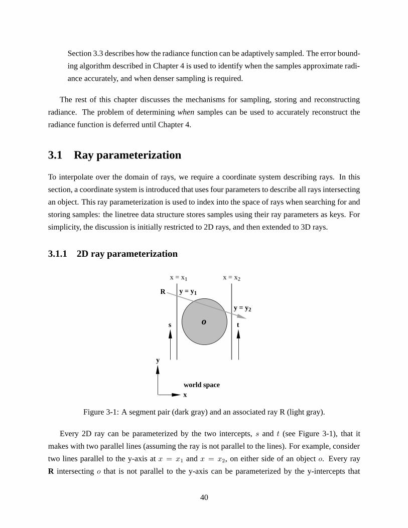
3.1 Ray parameterization . . . . . . . . . . . . . . . . . . . . . . . . . . . . . . . . . 40

3.1.1 2D ray parameterization . . . . . . . . . . . . . . . . . . . . . . . . . . . 40

3.1.2 3D ray parameterization . . . . . . . . . . . . . . . . . . . . . . . . . . . 43

3.1.3 Line space vs. ray space . . . . . . . . . . . . . . . . . . . . . . . . . . . 43

3.2 Interpolants and linetrees . . . . . . . . . . . . . . . . . . . . . . . . . . . . . . . 44

3.2.1 2D line space . . . . . . . . . . . . . . . . . . . . . . . . . . . . . . . . . 44

3.2.2 4D line space . . . . . . . . . . . . . . . . . . . . . . . . . . . . . . . . . 46

3.3 Using 4D linetrees . . . . . . . . . . . . . . . . . . . . . . . . . . . . . . . . . . 47

3.4 Comparing the base and interpolant ray tracers . . . . . . . . . . . . . . . . . . . 49

3.5 Discussion . . . . . . . . . . . . . . . . . . . . . . . . . . . . . . . . . . . . . . . 50

3.5.1 Efficient quadrilinear interpolation . . . . . . . . . . . . . . . . . . . . . . 50

3.5.2 Adaptive linetree subdivision . . . . . . . . . . . . . . . . . . . . . . . . . 51

3.5.3 Sharing sample rays . . . . . . . . . . . . . . . . . . . . . . . . . . . . . 52

3.5.4 Linetree depth . . . . . . . . . . . . . . . . . . . . . . . . . . . . . . . . 53

3.5.5 Linetree lookup cache . . . . . . . . . . . . . . . . . . . . . . . . . . . . 54

3.5.6 Alternative data structures . . . . . . . . . . . . . . . . . . . . . . . . . . 54

3.5.7 Alternative ray parameterizations . . . . . . . . . . . . . . . . . . . . . . 56

4 Error Bounds 57

4.1 Overview . . . . . . . . . . . . . . . . . . . . . . . . . . . . . . . . . . . . . . . 57

4.1.1 Interpolant validation . . . . . . . . . . . . . . . . . . . . . . . . . . . . . 58

4.1.2 Assumptions and limitations . . . . . . . . . . . . . . . . . . . . . . . . . 59

4.2 Radiance discontinuities . . . . . . . . . . . . . . . . . . . . . . . . . . . . . . . 59

4.2.1 Ray trees . . . . . . . . . . . . . . . . . . . . . . . . . . . . . . . . . . . 60

4.2.2 Invariant for discontinuities . . . . . . . . . . . . . . . . . . . . . . . . . 61

4.2.3 A taxonomy of discontinuities . . . . . . . . . . . . . . . . . . . . . . . . 62

4.2.4 Detecting discontinuities . . . . . . . . . . . . . . . . . . . . . . . . . . . 65

4.3 Non-linear radiance variations . . . . . . . . . . . . . . . . . . . . . . . . . . . . 74

4.3.1 Motivation . . . . . . . . . . . . . . . . . . . . . . . . . . . . . . . . . . 74

4.3.2 Local shading model . . . . . . . . . . . . . . . . . . . . . . . . . . . . . 75

4.3.3 Goal: bounding interpolation error . . . . . . . . . . . . . . . . . . . . . . 77

4.3.4 Interval arithmetic . . . . . . . . . . . . . . . . . . . . . . . . . . . . . . 78

4.3.5 Linear interval arithmetic . . . . . . . . . . . . . . . . . . . . . . . . . . . 79

4.3.6 Comparison of interval-based error bounding techniques . . . . . . . . . . 85

8

4.3.7 Application to the shading computation . . . . . . . . . . . . . . . . . . . 86

4.3.8 Error refinement . . . . . . . . . . . . . . . . . . . . . . . . . . . . . . . 91

4.4 Optimizations . . . . . . . . . . . . . . . . . . . . . . . . . . . . . . . . . . . . . 94

4.4.1 Error-driven subdivision . . . . . . . . . . . . . . . . . . . . . . . . . . . 94

4.4.2 Unique ray trees . . . . . . . . . . . . . . . . . . . . . . . . . . . . . . . 96

4.4.3 Textures . . . . . . . . . . . . . . . . . . . . . . . . . . . . . . . . . . . . 96

4.5 Extensions to scene and lighting models . . . . . . . . . . . . . . . . . . . . . . . 96

4.6 Discussion: error approximation . . . . . . . . . . . . . . . . . . . . . . . . . . . 98

5 Accelerating visibility 99

5.1 Temporal coherence . . . . . . . . . . . . . . . . . . . . . . . . . . . . . . . . . . 99

5.1.1 Reprojecting linetrees . . . . . . . . . . . . . . . . . . . . . . . . . . . . 100

5.1.2 Reprojection correctness . . . . . . . . . . . . . . . . . . . . . . . . . . . 103

5.1.3 Optimizations: adaptive shaft-culling . . . . . . . . . . . . . . . . . . . . 106

5.2 Image-space coherence . . . . . . . . . . . . . . . . . . . . . . . . . . . . . . . . 107

5.3 Progressive image refinement using extrapolation . . . . . . . . . . . . . . . . . . 108

5.3.1 Algorithm 1: Simple extrapolation . . . . . . . . . . . . . . . . . . . . . . 110

5.3.2 Algorithm 2: Extrapolation with correct visibility . . . . . . . . . . . . . . 110

5.3.3 Algorithms 3 and 4: Progressive refinement . . . . . . . . . . . . . . . . . 113

6 Scene Editing 115

6.1 Goal . . . . . . . . . . . . . . . . . . . . . . . . . . . . . . . . . . . . . . . . . . 116

6.1.1 The scene editing problem . . . . . . . . . . . . . . . . . . . . . . . . . . 116

6.1.2 Edits supported . . . . . . . . . . . . . . . . . . . . . . . . . . . . . . . . 117

6.1.3 Why use interpolants for scene editing? . . . . . . . . . . . . . . . . . . . 118

6.2 Ray dependencies . . . . . . . . . . . . . . . . . . . . . . . . . . . . . . . . . . . 119

6.2.1 Global line space parameterization . . . . . . . . . . . . . . . . . . . . . . 119

6.2.2 Line space affected by an object edit . . . . . . . . . . . . . . . . . . . . . 120

6.3 Interpolant dependencies . . . . . . . . . . . . . . . . . . . . . . . . . . . . . . . 121

6.3.1 Interpolant dependencies in world space . . . . . . . . . . . . . . . . . . . 122

6.3.2 Interpolant dependencies in global line space . . . . . . . . . . . . . . . . 124

6.4 Interpolants and ray segments . . . . . . . . . . . . . . . . . . . . . . . . . . . . 125

6.4.1 Limitations of line space . . . . . . . . . . . . . . . . . . . . . . . . . . . 125

6.4.2 Ray segment space . . . . . . . . . . . . . . . . . . . . . . . . . . . . . . 126

6.4.3 Global ray segment trees . . . . . . . . . . . . . . . . . . . . . . . . . . . 126

9

6.4.4 Inserting interpolants in the ray segment tree . . . . . . . . . . . . . . . . 127

6.5 Using ray segment trees . . . . . . . . . . . . . . . . . . . . . . . . . . . . . . . . 129

6.5.1 Identifying affected interpolants . . . . . . . . . . . . . . . . . . . . . . . 129

6.5.2 Interpolant invalidation . . . . . . . . . . . . . . . . . . . . . . . . . . . . 130

6.6 Discussion: pixel-based acceleration for scene editing . . . . . . . . . . . . . . . . 131

7 Performance Results 133

7.1 Base ray tracer . . . . . . . . . . . . . . . . . . . . . . . . . . . . . . . . . . . . 133

7.2 Test scene . . . . . . . . . . . . . . . . . . . . . . . . . . . . . . . . . . . . . . . 134

7.3 Timing results . . . . . . . . . . . . . . . . . . . . . . . . . . . . . . . . . . . . . 136

7.4 Memory usage and linetree cache management . . . . . . . . . . . . . . . . . . . 139

7.5 Scene editing . . . . . . . . . . . . . . . . . . . . . . . . . . . . . . . . . . . . . 141

7.6 Extrapolation . . . . . . . . . . . . . . . . . . . . . . . . . . . . . . . . . . . . . 143

7.7 Performance vs. image quality . . . . . . . . . . . . . . . . . . . . . . . . . . . . 144

7.8 Multi-processing . . . . . . . . . . . . . . . . . . . . . . . . . . . . . . . . . . . 146

8 Conclusions and Future Work 149

8.1 Contributions . . . . . . . . . . . . . . . . . . . . . . . . . . . . . . . . . . . . . 149

8.2 Future work and extensions . . . . . . . . . . . . . . . . . . . . . . . . . . . . . . 150

8.2.1 Animations and modeling . . . . . . . . . . . . . . . . . . . . . . . . . . 151

8.2.2 Architectural walk-throughs . . . . . . . . . . . . . . . . . . . . . . . . . 152

8.2.3 Intelligent, adaptive sampling . . . . . . . . . . . . . . . . . . . . . . . . 152

8.2.4 Perception-based error metrics . . . . . . . . . . . . . . . . . . . . . . . . 153

8.2.5 Generalized shading model, geometry and scene complexity . . . . . . . . 153

A Scene Editing: line space affected by an edit 157

A.1 Edits in two dimensions . . . . . . . . . . . . . . . . . . . . . . . . . . . . . . . . 158

A.2 Edits in three dimensions . . . . . . . . . . . . . . . . . . . . . . . . . . . . . . . 159

10

List of Figures

1-1 Coherence and the localized effect of an edit . . . . . . . . . . . . . . . . . . . . . 17

1-2 Whitted ray tracer . . . . . . . . . . . . . . . . . . . . . . . . . . . . . . . . . . . 19

1-3 High-level structure of the interpolant ray tracer . . . . . . . . . . . . . . . . . . . 20

1-4 Effectiveness of radiance interpolants . . . . . . . . . . . . . . . . . . . . . . . . 22

1-5 Algorithm overview . . . . . . . . . . . . . . . . . . . . . . . . . . . . . . . . . . 25

1-6 System overview . . . . . . . . . . . . . . . . . . . . . . . . . . . . . . . . . . . 27

3-1 A segment pair and an associated ray . . . . . . . . . . . . . . . . . . . . . . . . . 40

3-2 Two segment pairs and some associated rays . . . . . . . . . . . . . . . . . . . . . 41

3-3 Ray parameterization in 3D . . . . . . . . . . . . . . . . . . . . . . . . . . . . . . 42

3-4 Line space vs. ray space; radiance along ray R depends on the eye position . . . . . 43

3-5 A segment pair and its associated s-t line space . . . . . . . . . . . . . . . . . . . 45

3-6 A 2D segment pair and its children . . . . . . . . . . . . . . . . . . . . . . . . . . 46

3-7 A 4D linetree cell and its sixteen extremal rays . . . . . . . . . . . . . . . . . . . 47

3-8 Linetree cell subdivision . . . . . . . . . . . . . . . . . . . . . . . . . . . . . . . 48

3-9 Linetree visualization . . . . . . . . . . . . . . . . . . . . . . . . . . . . . . . . . 49

3-10 Comparing the base ray tracer and the interpolant ray tracer . . . . . . . . . . . . . 50

3-11 4-way split of linetree cell . . . . . . . . . . . . . . . . . . . . . . . . . . . . . . 52

3-12 Common rays . . . . . . . . . . . . . . . . . . . . . . . . . . . . . . . . . . . . . 53

3-13 A simplex in 2D and 3D . . . . . . . . . . . . . . . . . . . . . . . . . . . . . . . 55

4-1 A ray tree . . . . . . . . . . . . . . . . . . . . . . . . . . . . . . . . . . . . . . . 60

4-2 Visibility changes . . . . . . . . . . . . . . . . . . . . . . . . . . . . . . . . . . . 62

4-3 Occluders . . . . . . . . . . . . . . . . . . . . . . . . . . . . . . . . . . . . . . . 63

4-4 Shadows . . . . . . . . . . . . . . . . . . . . . . . . . . . . . . . . . . . . . . . . 63

4-5 Shading algorithm . . . . . . . . . . . . . . . . . . . . . . . . . . . . . . . . . . . 64

4-6 Least-common ancestor optimization for shaft culling . . . . . . . . . . . . . . . . 65

11

4-7 Shaft-culling for shadows . . . . . . . . . . . . . . . . . . . . . . . . . . . . . . . 66

4-8 Total internal reflection . . . . . . . . . . . . . . . . . . . . . . . . . . . . . . . . 67

4-9 Reflection of a convex object . . . . . . . . . . . . . . . . . . . . . . . . . . . . . 68

4-10 Construction of a bounding volume for reflected rays . . . . . . . . . . . . . . . . 69

4-11 Problem with spotlights . . . . . . . . . . . . . . . . . . . . . . . . . . . . . . . . 71

4-12 Spotlight: Test 1 . . . . . . . . . . . . . . . . . . . . . . . . . . . . . . . . . . . . 72

4-13 Spotlight: Test 2 . . . . . . . . . . . . . . . . . . . . . . . . . . . . . . . . . . . . 72

4-14 Spotlight: Test 3 . . . . . . . . . . . . . . . . . . . . . . . . . . . . . . . . . . . . 72

4-15 Spotlight: Test 4 . . . . . . . . . . . . . . . . . . . . . . . . . . . . . . . . . . . . 72

4-16 Non-linear radiance variations . . . . . . . . . . . . . . . . . . . . . . . . . . . . 75

4-17 Diffuse peak . . . . . . . . . . . . . . . . . . . . . . . . . . . . . . . . . . . . . . 76

4-18 Ray geometry . . . . . . . . . . . . . . . . . . . . . . . . . . . . . . . . . . . . . 76

4-19 Interpolation error . . . . . . . . . . . . . . . . . . . . . . . . . . . . . . . . . . . 78

4-20 The four linear bounding functions specified by a linear interval . . . . . . . . . . 79

4-21 Bounding maximum interpolation error . . . . . . . . . . . . . . . . . . . . . . . 80

4-22 Comparison of various error bounding techniques . . . . . . . . . . . . . . . . . . 86

4-23 A linetree cell for a surface patch in 3D . . . . . . . . . . . . . . . . . . . . . . . 87

4-24 A linetree cell for a surface patch in 2D . . . . . . . . . . . . . . . . . . . . . . . 89

4-25 Error refinement for a specular highlight . . . . . . . . . . . . . . . . . . . . . . . 92

4-26 Error refinement for a diffuse highlight . . . . . . . . . . . . . . . . . . . . . . . . 93

4-27 Error refinement for the museum scene . . . . . . . . . . . . . . . . . . . . . . . . 94

4-28 Actual and interpolated radiance . . . . . . . . . . . . . . . . . . . . . . . . . . . 95

4-29 Actual and conservative error bounds . . . . . . . . . . . . . . . . . . . . . . . . . 95

5-1 Pixels covered by a linetree cell . . . . . . . . . . . . . . . . . . . . . . . . . . . 101

5-2 Reprojection in 2D . . . . . . . . . . . . . . . . . . . . . . . . . . . . . . . . . . 102

5-3 Reprojection in 3D . . . . . . . . . . . . . . . . . . . . . . . . . . . . . . . . . . 102

5-4 Reprojection correctness . . . . . . . . . . . . . . . . . . . . . . . . . . . . . . . 103

5-5 Shaft cull for reprojection correctness . . . . . . . . . . . . . . . . . . . . . . . . 104

5-6 Reprojection algorithm . . . . . . . . . . . . . . . . . . . . . . . . . . . . . . . . 105

5-7 Reprojection algorithm with screen-space interpolation . . . . . . . . . . . . . . . 108

5-8 Reprojection for the museum scene . . . . . . . . . . . . . . . . . . . . . . . . . . 109

5-9 Extrapolation algorithm with correct visibility determination . . . . . . . . . . . . 111

5-10 Extrapolation for the museum scene: Algorithms 1 and 2 . . . . . . . . . . . . . . 112

5-11 Extrapolation for the museum scene: Algorithms 3 and 4 . . . . . . . . . . . . . . 114

12

6-1 Effect of a scene edit . . . . . . . . . . . . . . . . . . . . . . . . . . . . . . . . . 116

6-2 Interpolants for editing . . . . . . . . . . . . . . . . . . . . . . . . . . . . . . . . 119

6-3 Circle edit affects a hyperbolic region in line space . . . . . . . . . . . . . . . . . 120

6-4 Rectangle edit affects an hourglass region in line space . . . . . . . . . . . . . . . 121

6-5 Rays that affect an interpolant . . . . . . . . . . . . . . . . . . . . . . . . . . . . 122

6-6 Example: tunnel sections of interpolants . . . . . . . . . . . . . . . . . . . . . . . 123

6-7 Global line space for: (a) light rays, (b) reflected rays . . . . . . . . . . . . . . . . 124

6-8 Line space vs. ray segment space . . . . . . . . . . . . . . . . . . . . . . . . . . . 126

6-9 Interpolant dependencies in ray segment space . . . . . . . . . . . . . . . . . . . . 127

6-10 Subdivision of ray segment trees . . . . . . . . . . . . . . . . . . . . . . . . . . . 128

6-11 Dependencies for the reflective mirror in the museum scene . . . . . . . . . . . . . 130

7-1 Museum scene . . . . . . . . . . . . . . . . . . . . . . . . . . . . . . . . . . . . 135

7-2 Algorithm overview . . . . . . . . . . . . . . . . . . . . . . . . . . . . . . . . . . 137

7-3 Performance breakdown by rendering path and time . . . . . . . . . . . . . . . . . 138

7-4 Timing comparisons for 60 frames . . . . . . . . . . . . . . . . . . . . . . . . . . 139

7-5 Impact of linetree cache management on performance . . . . . . . . . . . . . . . . 140

7-6 Scene edits . . . . . . . . . . . . . . . . . . . . . . . . . . . . . . . . . . . . . . 142

7-7 Performance vs. quality in the interpolant ray tracer . . . . . . . . . . . . . . . . . 145

A-1 A hyperbolic region of line space corresponds to a circular region of world space . 157

13

Chapter 1

Introduction

A long-standing challenge in computer graphics is the rapid rendering of accurate, high-quality

imagery. Rendering algorithms generate images by simulating light and its interaction with the

environment, where the environment is modeled as a collection of virtual lights, objects and a

camera. The rendering algorithm is responsible for computing the path that light follows from the

light sources to the camera. The goal of this thesis is to develop a fast, high-quality rendering

algorithm that can be used in interactive applications.

Renderers that offer interactive performance, such as standard graphics hardware engines, per-

mit the scene to change dynamically and the user’s viewpoint to change. Hardware rendering

has become impressively fast; however, this interactive performance is achieved by sacrificing im-

age quality. Most hardware renderers use local illumination algorithms that render each object as

though it were the only one in the scene. As a result, these algorithms do not render effects such

as shadows or reflections, which arise from the lighting interactions between objects.

Global illumination algorithms, on the other hand, focus on producing the most realistic image

possible. These systems produce an image by simulating the light energy, or radiance, that is

visible at each pixel of the image. These algorithms improve rendering accuracy and permit higher

scene complexity than when a hardware renderer is used. However, computing the true equilibrium

distribution of light energy in a scene is very expensive. Therefore, practical global illumination

algorithms typically compromise the degree of realism to provide faster rendering. Two commonly

used global illumination algorithms span the spectrum of options: ray tracing and radiosity.

At one end of the spectrum, ray tracing [Whi80] is a popular technique for rendering high-

quality images. Ray tracers support a rich set of models and capture view-dependent specular

effects, as well as reflections and transmission. However, the view-dependent component of radi-

ance is expensive to compute, making ray tracers unsuitable for interactive applications.

15

At the other end, radiosity methods [GTGB84] capture view-independent diffuse inter-reflections

in a scene; however, these methods restrict the scene to pure diffuse, polygonal objects. Radiosity

systems pre-compute view-independentradiosity for all polygons in the scene, allowing the scene

to be rendered in hardware at interactive rates as the viewpoint changes.

Ideally, a rendering system would support interactive rendering of dynamically-changing scenes,

generating realistic, high-quality imagery. This thesis demonstrates an approach to accelerating

ray tracing so that a user can interact with the scene while receiving high-quality, ray-traced im-

agery as feedback.Two kinds of interactions are permitted: changes to the viewpoint, and changes

to the scene itself.

1.1 Applications

The rendering techniques presented in this thesis should be useful in a variety of different applica-

tions that incorporate interactive rendering, such as computer-aided design, architectural walk-

throughs, simulation and scientific visualization, generation of animations, virtual reality, and

games. In this section, a few of these applications are discussed.

For computer-aided design and modeling, a fast, high-quality renderer would allow the designer

to obtain accurate, interactive feedback about the objects being modeled. This feedback would

improve the efficiency of the design process. Architecture is one area of design where accurate

feedback on appearance is particularly useful, because the appearance of the product is central to

the design process. Because lighting effects such as shadows and reflections have a significant

impact on appearance, a renderer that takes global illumination into account is required.

Animated movies and computer-generated visual effects are usually produced using ray trac-

ers, and considerable computational expense is incurred to ensure that the rendered results do not

contain visible errors. The techniques introduced in this thesis are particularly appropriate for

the problem of rendering animations because they improve performance most when accelerating

a sequence of frames in which the scenes rendered in each frames are similar to one another. For

cinematic animations, it is important that rendering error be strictly controlled; this thesis also in-

troduces useful techniques for controlling error. The rendering techniques presented here should

improve the interactive design process for animations, and also accelerate rendering of the anima-

tion itself, although it is unrealistic at present to expect real-time rendering of the animation.

Faster rendering techniques would also be of use for scientific visualization and simulation.

High-quality rendering of results of a simulation—for example, an aerodynamic simulation or a

detailed molecular simulation—can make the results easier to grasp intuitively, both during the

16

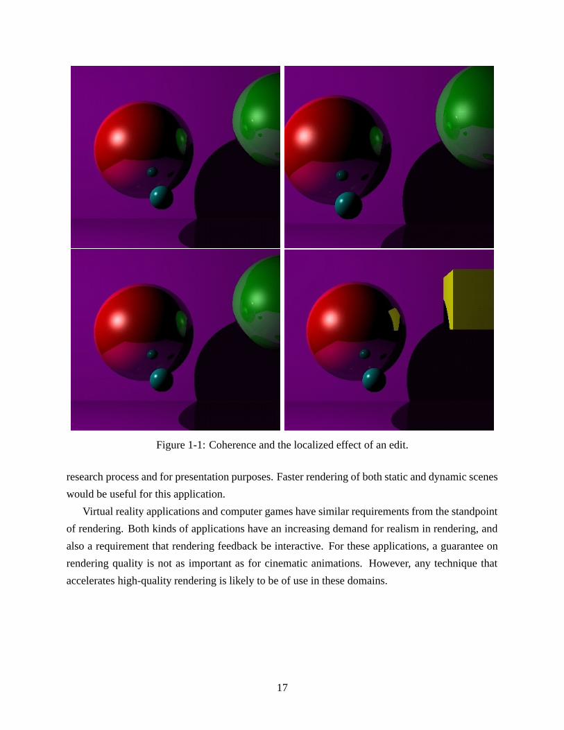
Figure 1-1: Coherence and the localized effect of an edit.

research process and for presentation purposes. Faster rendering of both static and dynamic scenes

would be useful for this application.

Virtual reality applications and computer games have similar requirements from the standpoint

of rendering. Both kinds of applications have an increasing demand for realism in rendering, and

also a requirement that rendering feedback be interactive. For these applications, a guarantee on

rendering quality is not as important as for cinematic animations. However, any technique that

accelerates high-quality rendering is likely to be of use in these domains.

17

1.2 Intuition

The key observation for acceleration of ray tracing is that radiance tends to be a smoothly varying

function. A ray tracer ought to be able to exploit this smoothness in radiance to compute radiance

without doing the full work of ray tracing every pixel in the image independently.

This central intuition is illustrated in Figure 1-1. On the top row are two images shown from

two nearby viewpoints. On the bottom row are two images shown from the same viewpoint; these

images show a scene that is edited by replacing the green sphere with a yellow cube. There are

several points of interest:

• First, consider only the image on the top left. Radiance varies smoothly along the objects in

the image except at a few places such as specular highlights and silhouettes. This smoothness

is called object-space coherence.

• When these objects are rendered to produce an image, nearby pixels in the image have similar

radiance values. This is called image-space coherence.

• Now consider the image on the top right, where the viewpoint has changed with respect to the

image on the top left. If the viewpoint changes by a small amount, the radiance information

computed for the previous frame can be reused in the new frame. This is called temporal

coherence.

• Finally, when the user edits the scene shown in the bottom row of the figure, only a small

part of the ray-traced image is affected: the green sphere and its reflection. The rest of the

image remains the same. The effect of the edit is localized; this property will be referred to

as the localized-effect property.

This thesis introduces new mechanisms that allow a ray tracer to exploit object-space, image-

space, and temporal coherence to accelerate rendering. Coherence allows the radiance for many

pixels in the image to be approximated using already-computed radiance information. Using these

various intuitions, rendering can be accelerated in various ways:

• Ray tracing of static scenes can be accelerated by exploiting object-space and image-space

coherence within a single frame. Further acceleration can be achieved by exploiting temporal

coherence across multiple frames, as the user’s viewpoint changes.

• When the scene is not static, the localized-effect property allows the scene to be incremen-

tally re-rendered even when the scene is allowed to change. These changes may include

moving, adding, or deleting objects in the scene.

18

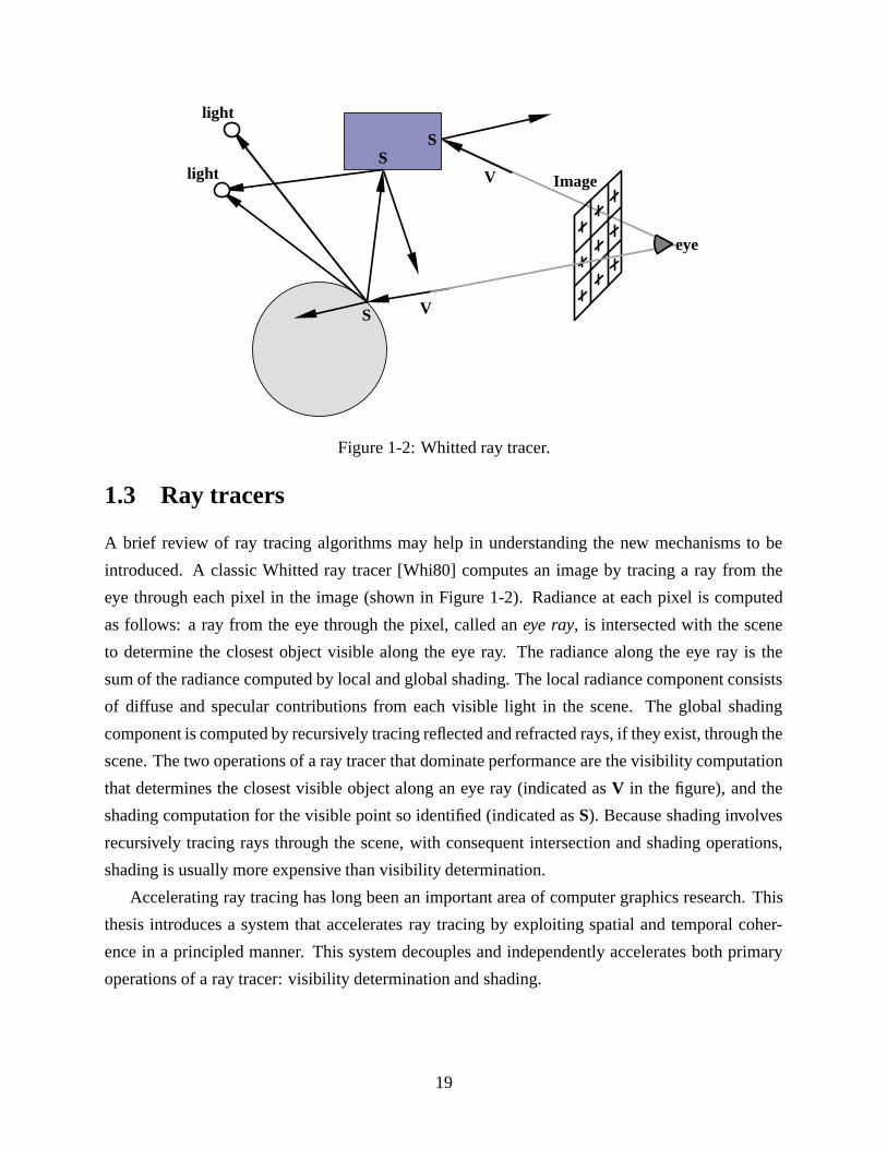
V

light

Image

S

eye

light V

SS

Figure 1-2: Whitted ray tracer.

1.3 Ray tracers

A brief review of ray tracing algorithms may help in understanding the new mechanisms to be

introduced. A classic Whitted ray tracer [Whi80] computes an image by tracing a ray from the

eye through each pixel in the image (shown in Figure 1-2). Radiance at each pixel is computed

as follows: a ray from the eye through the pixel, called an eye ray, is intersected with the scene

to determine the closest object visible along the eye ray. The radiance along the eye ray is the

sum of the radiance computed by local and global shading. The local radiance component consists

of diffuse and specular contributions from each visible light in the scene. The global shading

component is computed by recursively tracing reflected and refracted rays, if they exist, through the

scene. The two operations of a ray tracer that dominate performance are the visibility computation

that determines the closest visible object along an eye ray (indicated as V in the figure), and the

shading computation for the visible point so identified (indicated as S). Because shading involves

recursively tracing rays through the scene, with consequent intersection and shading operations,

shading is usually more expensive than visibility determination.

Accelerating ray tracing has long been an important area of computer graphics research. This

thesis introduces a system that accelerates ray tracing by exploiting spatial and temporal coher-

ence in a principled manner. This system decouples and independently accelerates both primary

operations of a ray tracer: visibility determination and shading.

19

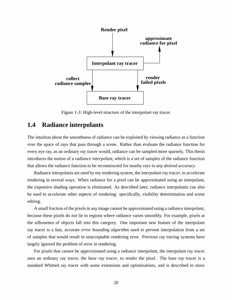
collectradiance samples

render failed pixels

Interpolant ray tracer

Base ray tracer

Render pixel

approximate radiance for pixel

Figure 1-3: High-level structure of the interpolant ray tracer.

1.4 Radiance interpolants

The intuition about the smoothness of radiance can be exploited by viewing radiance as a function

over the space of rays that pass through a scene. Rather than evaluate the radiance function for

every eye ray, as an ordinary ray tracer would, radiance can be sampled more sparsely. This thesis

introduces the notion of a radiance interpolant, which is a set of samples of the radiance function

that allows the radiance function to be reconstructed for nearby rays to any desired accuracy.

Radiance interpolants are used by my rendering system, the interpolant ray tracer, to accelerate

rendering in several ways. When radiance for a pixel can be approximated using an interpolant,

the expensive shading operation is eliminated. As described later, radiance interpolants can also

be used to accelerate other aspects of rendering: specifically, visibility determination and scene

editing.

A small fraction of the pixels in any image cannot be approximated using a radiance interpolant,

because these pixels do not lie in regions where radiance varies smoothly. For example, pixels at

the silhouettes of objects fall into this category. One important new feature of the interpolant

ray tracer is a fast, accurate error bounding algorithmused to prevent interpolation from a set

of samples that would result in unacceptable rendering error. Previous ray tracing systems have

largely ignored the problem of error in rendering.

For pixels that cannot be approximated using a radiance interpolant, the interpolant ray tracer

uses an ordinary ray tracer, the base ray tracer, to render the pixel. The base ray tracer is a

standard Whitted ray tracer with some extensions and optimizations, and is described in more

20

detail in Chapters 4 and 7. The base ray tracer is also used by the interpolant ray tracer to collect

the samples that make up interpolants. The interface between these two ray tracers is depicted in

Figure 1-3. The goal of the interpolant ray tracer is to produce an image that closely approximates

the image produced by the base ray tracer, but more quickly than the base ray tracer would.

Figure 1-4 shows images of how successful interpolants are at exploiting coherence. In the left

column, rendered output of the ray tracer is shown. In the right column, color-coded images show

in blue the pixels that are reconstructed using interpolants. Green, yellow, and pink pixels show

where interpolants are not used, because radiance was not known to vary smoothly. Two important

observations can be made about the color-coded images. First, most of the pixels are blue, so

rendering is accelerated; for this image, rendering is about 5 times faster with the interpolant ray

tracer. Second, interpolation is correctly avoided where it would produce inaccurate results.

The second row shows the same scene from a nearby viewpoint. The red pixels on the right

show pixels for which no previously computed radiance interpolant (from the image on top) was

suitable for computing their radiance. These pixels are rendered using radiance interpolants that are

computed on the fly as the image is being rendered; despite the computation of new interpolants,

the rendering of these pixels is still accelerated when compared to the base ray tracer. Note that

the radiance for most pixels can be computed using radiance interpolants from the image on top.

Thus, temporal coherence is effectively exploited in this example.

The bottom row shows results for a scene edit. Note that most of the image is unaffected by

the edit and is rendered using previously constructed interpolants. Radiance is affected by the edit

only for the pixels marked in red, which are correctly identified by the ray tracer. The image is

then rendered incrementally, reusing all the unaffected radiance interpolants computed earlier.

Radiance interpolants are the central mechanism used by the interpolant ray tracer. They are

used to accelerate both primary operations of a ray tracer: visibility determination and shading.

They are also useful when incrementally re-rendering a dynamic scene. The next three sections

discuss these uses of radiance interpolants in more detail.

1.4.1 Accelerating shading

As described, the interpolant ray tracer accelerates shading by using a suitable interpolant to ap-

proximate the radiance of the pixel, rather than performing the usual shading operation. If no

information is available about the radiance function, interpolating radiance samples can introduce

arbitrary errors in the image. Therefore, it is necessary to characterize how radiance varies over

ray space. Systems that exploit coherence to accelerate rendering have traditionally used ad hoc

techniques to determine where to sample radiance; these systems have no correctness guarantees.

21

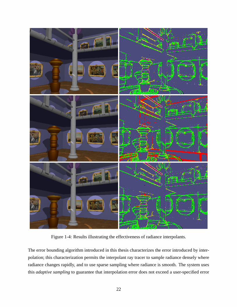
Figure 1-4: Results illustrating the effectiveness of radiance interpolants.

The error bounding algorithm introduced in this thesis characterizes the error introduced by inter-

polation; this characterization permits the interpolant ray tracer to sample radiance densely where

radiance changes rapidly, and to use sparse sampling where radiance is smooth. The system uses

this adaptive samplingto guarantee that interpolation error does not exceed a user-specified error

22

bound ε. The user can use ε to control performance-quality trade-offs.

1.4.2 Accelerating visibility

Visibility determination is accelerated by exploiting frame-to-frame temporal coherence: when the

viewpoint changes, objects visible in the previous frame are still typically visible in the current

frame, as discussed in Section 1.2. This occurs because eye rays from the new viewpoint are close

(in ray space) to eye rays from the previous viewpoint. When the interpolant ray tracer is used to

render a sequence of frames from nearby viewpoints, interpolants from one frame are reprojected

to the next frame. A reprojected interpolant covers some set of pixels in the new frame; these

pixels are rendered using the interpolant. Rendering is substantially accelerated because neither

visibility nor shading is explicitly computed for these pixels.

1.4.3 Incremental rendering with scene editing

Conventional ray tracers are too slow to be used for interactive modeling. In this application, when

a user edits a scene, he should quickly receive high-quality rendered imagery as feedback. Rapid

feedback in such scenarios is a reasonable expectation because the effect of an edit is typically

localized (as described in Section 1.2); therefore, rendering a slightly modified scene could be

much faster than rendering the original image. However, conventional ray tracers do not exploit

this fact. An incrementalrenderer that efficiently identifies and updates the pixels affected by an

edit would enable the user to get rapid high-quality feedback.

Identifying the pixels affected by an edit is not easy; therefore, researchers have supported

scene editing with ray tracing by restricting the viewpoint to a fixed location [SS89, BP96]. These

systems permit a limited set of edits, such as color changes and object movement. However, if the

user changes the viewpoint, the whole frame is re-rendered, incurring the cost of pre-processing

to support edits from the new viewpoint. This restriction on the viewpoint limits the usefulness of

these systems.

This thesis describes how radiance interpolants can be used to support incremental rendering

with scene editing, while allowing the viewpoint to change. The interpolant ray tracer constructs

interpolants, which are useful for scene editing for the following two reasons. First, an interpolant

represents a bundle of rays. Therefore, updating an interpolant efficiently updates radiance for all

the rays represented by the interpolant. Second, an interpolant does not depend on the viewpoint.

Therefore, interpolants are not invalidated when the viewpoint changes.

The incremental renderer supports edits such as changing the material properties of objects in

23

the scene, adding/deleting/moving objects, and changing the viewpoint. When the user edits the

scene, the system automatically identifies the interpolants that are affected by the edit. Unaffected

interpolants are used when re-rendering the scene.

1.5 System overview

This section describes the flow of control in the interpolant ray tracing system and the data struc-

tures built during rendering. Some limitations of the system are also discussed.

1.5.1 Interpolant ray tracer

The interpolant ray tracer is the core of the system; it accelerates rendering by substituting interpo-

lation of radiance for ray tracing when possible. This section briefly describes how the interpolant

ray tracer accelerates ray tracing; the next section describes how the rest of the system is built

around the interpolant ray tracer.

Radiance samples collected by invoking the base ray tracer are used to construct interpolants,

which are stored in a data structure called a linetree. Each object has a set of associated linetrees

that store its radiance samples. The linetree has a hierarchical tree organization that permits the

efficient lookup of interpolants for each eye ray. Chapter 3 presents linetrees in detail.

Figure 1-5 shows the rendering algorithm of the interpolant ray tracer. Each pixel in the image

is rendered using one of three rendering paths: the fast path, the interpolate path, or the slow

path. Along the fast path, the system exploits frame-to-frame temporal coherence by reprojecting

interpolants from the previous frame; this accelerates both visibility and shading for pixels covered

by reprojected interpolants. Rendering of pixels that are not reprojected may still be accelerated

by interpolating radiance samples from the appropriate interpolants (interpolate path). If both

reprojection and interpolation fail for a pixel, the base ray tracer renders the pixel (slow path).

The fast path, indicated by the thick line, corresponds to the case when reprojection succeeds.

When a reprojected interpolant is available for a pixel, the system finds all consecutive pixels in

that scan-line covered by the same interpolant, and interpolates radiance for these pixels in screen-

space; neither the visibility nor shading computation is invoked for these pixels. This fast path

is about 30 times faster than the base ray tracer (see Chapter 7 for details), and is used for most

pixels.

If no reprojected interpolant is available, the eye ray is intersected with the scene to determine

the object visible at that pixel. The system searches for a valid interpolant for that ray and object

in the appropriate linetree; if it exists, the radiance for that eye ray (and the corresponding pixel) is

24

For every pixel pin image

Yes

Visibility

Shading

Reproject interpolantsfrom previous frame

No

Intersect eye raywith scene

Is there a reprojected interpolant?

Hit object o

Yes No

Interpolate pixel

Valid interpolant in o’s linetree?

Yes No

Collect samples tobuild interpolant

Interpolate pixel Base ray tracer

Interpolatespan

Check interpolant validity(error < ε)?

Interpolate path

Fast path

Slow path

Figure 1-5: Algorithm overview.

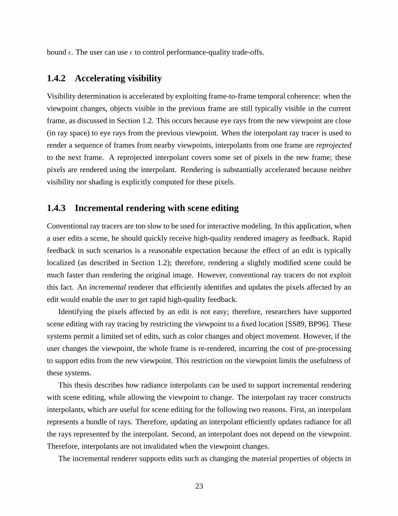
computed by quadrilinear interpolation. This interpolate path, indicated by the medium-thick line,

is about 5 times faster than the base ray tracer.

If an interpolant is not available for a pixel, the system builds an interpolant by collecting

radiance samples. The error bounding algorithm checks the validity of the new interpolant. If the

interpolant is valid, the pixel’s radiance can be interpolated, and the interpolant is stored in the

linetree. If it is not valid, the linetree is subdivided, and the system falls back to shading the pixel

using the base ray tracer. This is the slow path indicated by the thin black line.

Interpolation errors arise from discontinuities and non-linearities in the radiance function. The

error bounding algorithm automatically detects both these conditions. An interpolant is not con-

structed if the error bounding algorithm indicates conservatively that its interpolation error would

25

exceed a user-specified bound. Thus, linetrees are subdivided adaptively: sampling is sparse where

radiance varies smoothly, and dense where radiance changes rapidly. This adaptive subdivision of

linetrees prevents erroneous interpolation while allowing interpolant reuse when possible.

The interpolant ray tracer has the important property that it is entirely on-line: no pre-processing

is necessary to construct radiance interpolants, yet rendering of even the first image generated by

the ray tracer is accelerated. Radiance interpolants are generated lazily and adaptively as the scene

is rendered from various viewpoints. This on-line property is useful for interactive applications.

1.5.2 System structure

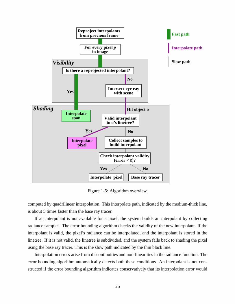
Figure 1-6 shows how the different components of the system, including the interpolant ray tracer,

fit together. In the figure, the rectangles represent code modules, and the ellipses represent the

data structures built in the course of rendering. Solid arrows indicate the flow of control, and

dotted arrows indicate the flow of data within the system. For example, the dotted arrow from the

“Linetree” ellipse to the “Reprojection” and “Interpolation” modules indicates that these modules

read data from the linetree, as described in Section 1.5.1. The dotted arrow from “Interpolant

construction” to “Linetree” indicates that this module writes data into the linetree.

The user interface module processes user input. Two kinds of user input are of interest: changes

in the viewpoint, and edits to the scene. If the user’s viewpoint changes, the interpolant ray tracer

renders an image from the new viewpoint, as described in Section 1.5.1. If the user edits the scene,

by changing the material properties of objects, or deleting objects, the “Scene Editing” module is

invoked.

The “Interpolant Ray Tracer” module has already been described in some detail. One additional

component is the memory management module, which bounds the memory usage of the ray tracer.

This module is invoked when the ray tracer requires more memory to construct interpolants than

is available. Using a least-recently-used scheme described in Chapter 7, the memory management

module identifies and frees linetree memory that can be reused.

The “Scene Editing” module provides the ability to incrementally update interpolants after a

user-specified change to the scene. A data structure called a ray segment tree(RST) is used to

record the regions of world space on which each interpolant depends. When an interpolant is

constructed, the “RST Update” module records the dependencies of the interpolant in ray segment

trees. When the user edits the scene, the ray segment trees are traversed to rapidly identify the

affected interpolants and invalidate them, removing them from the containing linetree. The new

image can then be rendered by the interpolant ray tracer, making use of any interpolants unaffected

by the edit.

26

Change inviewpoint

Scene editUser interface

Interpolant Ray Tracer

Reprojection

Interpolation

Interpolant construction

Error bounding

Base ray tracer

Linetree Ray segment tree

RST update

Invalidation ofaffected interpolants

Memory management

Scene Editing

Figure 1-6: System overview.

1.5.3 Limitations

To bound interpolation error the interpolant ray tracer makes several assumptions about the shad-

ing model and geometry of objects in the scene. These assumptions are discussed in detail in

Section 4.1.2. Because the interpolant ray tracer is an accelerated version of a Whitted ray tracer,

it inherits some of the limitations of a Whitted ray tracer. It also places some additional restrictions

on the scene being rendered.

The ray tracer uses the Ward isotropic shading model [War92]. While this is a more sophisti-

cated model than that of Whitted, it does not model diffuse inter-reflections and generalized light

transport. Also, the error bounding algorithm described in Chapter 4 requires that all objects be

convex, although some constructive solid geometry operators (union and intersection) are per-

mitted. Material properties may include diffuse texture maps, but not some more sophisticated

texturing techniques. The major reason for these limitations is to simplify the problem of conser-

27

vatively bounding error. Section 4.5 discusses approaches for bounding error in a system in which

these limitations are relaxed.

1.6 Contributions

In designing and building this system, this thesis makes several new contributions:

• Radiance interpolants:The system demonstrates that radiance can be approximated rapidly

by quadrilinear interpolation of the radiance samples in an interpolant.

• Linetrees:A hierarchical data structure called a linetree is used to store interpolants. The

appropriate interpolant for a particular ray from the viewpoint is located rapidly by walk-

ing down the linetree. Linetrees are subdivided adaptively (and lazily), thereby permitting

greater interpolant reuse where radiance varies smoothly, and denser sampling where radi-

ance changes rapidly.

• Error bounds:New techniques for bounding interpolation error are introduced. The system

guarantees that when radiance is approximated, the relative error between interpolated and

true radiance (as computed by the base ray tracer) is less than a user-specified error bound

ε. The user can vary the error bound ε to trade performance for quality. Larger permitted

error produces lower-quality images rapidly, while smaller permitted error improves image

quality at the expense of rendering performance.

Interpolation error arises both from discontinuities and non-linearities in the radiance func-

tion. An error bounding algorithm automatically and conservatively prevents interpolation in

both these cases. This algorithm uses a generalization of interval arithmetic to bound error.

• Error-driven sampling: The error bounding algorithm is used to guide adaptive subdivi-

sion; where the error bounding algorithm indicates rapid variations in radiance, radiance is

sampled more densely.

• Visibility by reprojection:Determination of the visible surface for each pixel is accelerated

by a novel reprojection algorithm that exploits temporal frame-to-frame coherence in the

user’s viewpoint, but guarantees correctness. A fast scan-line algorithm uses the reprojected

linetrees to further accelerate rendering.

• Memory management:Efficient cache management keeps the memory footprint of the sys-

tem small, while imposing a negligible performance overhead (1%).

28

• Interpolants for scene editing:The system demonstrates that interpolants provide an efficient

mechanism for incremental update of radiance when the scene is edited. This is possible

because the error bounding algorithm guarantees that each interpolant represents radiance

well for a region of ray space.

• Ray segment trees:The concept of ray segment space is introduced for scene editing. A

shaft in 3D space is represented simply as a bounding box in this five-dimensional space.

This concept is used to identify the regions of world space that affect an interpolant. An

auxiliary data structure, the ray segment tree, is built over ray segment space; when the

scene is edited, ray segment trees are rapidly traversed to identify affected interpolants.

1.7 Organization of thesis

The rest of the thesis is organized as follows: Chapter 2 discusses previous work. Chapter 3 de-

scribes the interpolant building mechanism and the linetree data structure in detail. Chapter 4

presents the error bounding algorithm, which validates interpolants and guarantees that interpola-

tion error does not exceed a user-specified error bound. Chapter 5 describes how reprojection is

used to accelerate visibility. Chapter 6 extends the interpolant ray tracer to support incremental

rendering with scene editing. Finally, Chapter 7 presents results and Chapter 8 concludes with a

discussion of future work.

29

Chapter 2

Related Work

This chapter presents the related work in accelerating ray tracing and incremental scene editing.

Section 2.1 discusses the most relevant prior work on accelerating high-quality renderers. Sec-

tion 2.2 presents related work on incremental rendering for scene editing with global illumination.

The contributions of this thesis are discussed in the context of previous work in Section 2.3.

2.1 Accelerating rendering

Accelerating rendering is a long standing area of research. Many researchers have developed tech-

niques that improve the performance of rendering systems: adaptive 3D spatial hierarchies [Gla84],

beam-tracing for polyhedral scenes [HH84], cone-tracing [Ama84], and ray classification [AK87].

A good summary of these algorithms can be found in [Gla89, CW93, SP94, Gla95]. In this chapter,

the related work most relevant to this thesis is presented.

Ray tracers perform two major operations: visibility determination and shading. Most sys-

tems presented here focus on accelerating shading, though a few systems exclusively accelerate

visibility determination. The distinction between these two objectives is often blurred, since both

improve the performance of rendering. Systems that accelerate rendering by approximating radi-

ance typically differ in the following ways:

• the correctness guarantees (if any) provided for computed radiance,

• the shading model supported,

• the use of pre-processing (if any), and

• the hardware expectations for performance.

31

Some of these systems also approximate visibility by polygonalizing the scene, or by using images

instead of geometry.

2.1.1 Systems with error estimates

Some rendering systems trade accuracy for speed by using error estimates to determine where

computation and memory resources should be expended. Some radiosity systems use explicit error

bounds to make this trade-off [HSA91, LSG94]. Ray tracers typically use stochastic techniques to

estimate error in computed radiance [Coo86, PS89] but do not rigorously bound error.

Ward’s RADIANCE ray tracer estimates error for diffuse radiance [WH92]. RADIANCE uses

ray tracing to produce high-quality images that include view-dependent specular effects, as well

as diffuse inter-reflections [WRC88, War92]. RADIANCE assumes that the diffuse component

of radiance varies slowly, and can be sampled sparsely. Therefore, the RADIANCE ray tracer

computes the specular radiance at each pixel, but lazily samples diffuse inter-reflections. The

system uses gradient information to guide the sparse, non-uniform sampling of the slowly-varying

diffuse component of radiance. However, RADIANCE does not interpolate the view-dependent

components of radiance, nor does it bound error incurred by its interpolation of sparse samples.

Several researchers exploit image coherence to accelerate ray tracing [AF84]. These systems

typically use error estimates based on the variance in pixel radiance to determine where to expend

computational resources. Recently, two systems that exploit image coherence for the progressive

refinement of ray-traced imagery have been developed [Guo98, PLS97]. These systems do not use

explicit error estimates, but implicitly try to decrease perceived error in the image by detecting

discontinuities in screen space. Guo [Guo98] samples the image sparsely along discontinuities

to produce images for previewing. For polyhedral scenes, Pighin et al. [PLS97] compute image-

space discontinuities, which are used to construct a constrained Delaunay triangulation of the im-

age plane. This Delaunay triangulation drives a sparse sampling technique to produce previewable

images rapidly. The traditional problem with screen-space interpolation techniques is that they

may incorrectly interpolate across small geometric details, radiance discontinuities, and radiance

non-linearities. While both these systems alleviate the problem of interpolation across disconti-

nuities, neither system bounds error. Since they do not guarantee error bounds, they are useful

for previewing; however, the user cannot be sure of obtaining an accurate image until the entire

image is rendered. Also, both systems detect discontinuities in the image plane; therefore, when

the viewpoint changes, discontinuities have to be recomputed from scratch.

32

2.1.2 Systems without error estimates

Several systems accelerate rendering by approximating visibility and shading, but do not use error

estimates or guarantee bounded error.

Hardware-based rendering. Some systems exploit the graphics hardware to obtain some of the

realism of ray tracing. Diefenbach’s rendering system [DB97] uses multiple passes of standard

graphics hardware to approximate ray-tracing effects such as shadows, reflections, and translu-

cency at interactive rates. Ofek and Rappoport [OR98] consider a particular sub-problem, reflec-

tions of objects in curved reflectors, and compute better approximations for this sub-problem. Both

systems use the graphics hardware to merge approximated reflections, shadows etc. with images at

interactive rates. While both these systems approximate ray-tracing effects, neither provides any

correctness guarantees. These systems are also restricted to polygonal scenes.

Parker et al. [PMS+99] use a “brute-force” approach to support interactive ray tracing on multi-

processors. Their approach focuses on software engineering issues in constructing a fast ray tracer.

Note that this approach does not approximate shading and computes accurate radiance at each

pixel, but relies on the computational power of multiprocessor hardware to accelerate rendering.

Image-based rendering. The goal of image-based rendering [MB95] is to support interactive

rendering of scenes where radiance samples are collected by acquiring images of the scene in

a pre-processing phase. The idea is to eliminate the scene model, and use images as the input

to the rendering engine. The interpolant ray tracer differs in its goals substantially from these

systems; however, IBR systems such as the Light Field [LH96] and the Lumigraph [GGSC96]

have similarities to the interpolant ray tracer because they also collect radiance samples over a

four-dimensional line space and quadrilinearly interpolate the samples to approximate radiance.

Both these IBR systems construct uniformly subdivided 4D arrays whose size is fixed in the pre-

processing phase. This fixed sampling rate does not guarantee that enough samples are collected in

regions with high-frequency radiance variations, and may result in over-sampling in regions where

radiance is smooth. Also, these systems typically constrain the viewpoint to lie outside the convex

hull of the scene.

Recently, Lischinski and Rappoport use layered depth images (LDIs) to rapidly render both dif-

fuse and specular radiance for new viewpoints [LR98]. They represent diffuse radiance with a few

high-resolution LDIs and specular radiance with several low-resolution LDIs. When the scene is

rendered, these LDIs are rapidly recombined to produce approximations to the correct image. For

small scenes, this approach has better memory usage and visual results than the light field or Lu-

migraph. However, scenes with greater depth complexity could require excessive memory. Also,

33

though this technique alleviates artifacts for specular surfaces, it still relies on radiance sampling

that is not error-driven.

Mark et al. [MMB97] apply a 3D warp to pixels from reference images to create an image

at the new viewpoint. They treat their reference image as a mesh and warp the mesh triangles

to the current viewpoint. Their system does not handle view-dependent shading such as specular

highlights and does not guarantee correct results for arbitrary movements of the eye.

Chevrier [Che97] computes a set of key views used to construct a 3D mesh that is interpolated

for new viewpoints. If a pixel is not covered by one key view, several key views are used. To

handle specularity, one 3D mesh per specular surface is built, and the specular coefficient is linearly

interpolated from multiple key images. While this algorithm decreases some aliasing artifacts, it

still may interpolate across shadows or specular highlights.

None of these image-based systems bounds the error introduced by approximating visibility

or radiance. Also, all these techniques require a pre-processing phase in which light fields, LDIs,

reference images, or key views are computed to be reused later. The memory requirements of these

systems is proportional to the number of reference images obtained in the pre-processing phase;

some systems use compression to alleviate this problem. Note that the reliance of these systems

on pre-processing precludes their use in interactive applications in which the scene changes.

2.1.3 Accelerating animations

By reusing information from frame to frame, several systems accelerate animations. Algorithms

that exploit temporal coherence to approximate visibility at pixels can be categorized by the as-

sumptions they make about the scene and the correctness guarantees they provide. Chapman et al.

use the known trajectory of the viewpoint through the scene to compute continuous intersection

information for rays [CCD90, CCD91]. However, because the system assumes that the scene is

polygonal and the paths of objects through the scene is known a priori, this system is not useful in

applications where the user interacts with the scene.

Several systems reuse pixels from the previous frame to render the current frame without any

prior knowledge of the viewpoint’s trajectory [Bad88, AH95]. Adelson and Hodges [AH95] apply

a 3D warp to pixels from reference images to the current image. Diffuse radiance is reused in

the warped pixels, but specular radiance is computed by casting rays as necessary. Their system

achieves modest performance benefits (on the order of 50%-70%), and exhibits aliasing effects

because pixels are not warped to pixel centers in the current frame.

Nimeroff et al. [NDR95] use IBR techniques to warp pre-rendered images in animated en-

vironments with moving viewpoints. However, their system does not provide any correctness

34

guarantees.

2.1.4 Higher-dimensional representations

Another related area of research is the use of line or ray space to accelerate rendering in global

illumination algorithms. Arvo and Kirk [AK87] represent bundles of rays as 5D bounding volumes

that are used to accelerate ray-object intersections. However, the focus of their work is to improve

the performance of visibility determination, and they do not accelerate shading or editing.

2.1.5 Radiance caching

Like the interpolant ray tracer, some systems cache radiance while rendering a frame and reuse

these cached radiance values to render interactively. Ward [War98] uses a 4D holodeckdata struc-

ture that is populated as the RADIANCE system computes an image. Walter et al. [WDP99] store

radiance samples in a render cache, and reproject these samples when the viewpoint changes.

With varying success, these systems use heuristics to fill in pixels not stored in their caches. These

systems focus on rendering speed, and so they do not characterize or bound the rendering errors

introduced by the heuristics they use.

2.2 Interactive scene editing

Recently, there has been increased interest in the problem of accelerating scene editing with various

global illumination algorithms. Work on both incremental ray tracers and incremental radiosity

algorithms is relevant to this thesis.

2.2.1 Ray tracing

Strides have been made in facilitating interactive scene manipulation with ray tracing. Several

researchers have developed ray tracers supporting scene editing that incrementally render only

those parts of the scene that might be affected by a change.

Cook’s shade trees[Coo84] maintain a symbolic evaluation of the local illumination at each

pixel of a frame. When an object’s material properties are changed, the shade trees are re-evaluated

with the new material properties, if they remain the same. Sequin and Smyrl [SS89] extend shade

trees to include reflections and refractions. Their ray treesrepresent the entire radiance contribution

by the scene at each pixel. When the user changes the material properties of objects (e.g., color,

35

specular coefficient) or changes light intensities, the affected trees are re-evaluated. However, this

approach assumes that the trees do not change by the scene edit; therefore, edits such as moving

an object or changing the viewpoint are not supported.

Murakami and Hirota [MH92] and Jevans [Jev92] extend these techniques to support geometry

changes such as moving an object in the scene, or deleting objects. Rays that are traced through

the scene during rendering are associated with the voxels they traverse. When the scene is edited,

the affected voxels and their associated rays are found. Radiance along the rays is then updated to

reflect the edit.

Recently, Briere and Poulin [BP96] introduced a system that supports incremental rendering for

a fixed viewpoint. Their system supports the most comprehensive set of edits to date. These edits

are categorized into two major types: attribute changes which involve adjustments to an object’s

color, reflection coefficient, and other material properties; and geometry changes, which include

changes such as moving an object. Color treesand ray treesare maintained for each pixel in the

image. These trees are used to separately accelerate updates to object attributes and geometry;

attribute edits typically only affect the color trees, while geometry edits affect both types of trees.

For efficiency, their system groups these trees and maintains hierarchical bounding volumes to

rapidly identify the pixels affected by an edit. Their system reflects attribute changes in about 1-2

seconds, and geometry changes in 10-110 seconds.

All of the above systems are completely view-dependent because they assume that the view-

point is fixed; while a user can edit the scene, he cannot adjust the viewpoint. Since the viewpoint

is fixed, all the techniques are pixel-based; that is, additional information, such as ray trees, are

maintained for each pixel in the image and used to recompute radiance as the user edits the scene.

Most of these systems use compression techniques to alleviate memory usage; even so, for high

resolution images, the memory requirements of these systems can be large.

2.2.2 Radiosity

In the context of radiosity, several researchers have studied the problem of dynamic editing [Che90,

GSG90, FYT94]. Recently, Dretakkis and Sillion [DS97] augment the link structure of hierarchical

radiosity with additional line-space information to track links affected by the addition or deletion

of objects. The hierarchical link structure, and hence the implicit line space, makes it possible

to identify affected regions rapidly when an object is edited. Their system is not pixel-based;

therefore, a user can change the viewpoint after an update. However, their algorithms apply only

to radiosity systems for scenes with diffuse materials.

36

2.3 Discussion

This thesis differs from previous work in several ways. The most important difference is that ra-

diance interpolants approximate radiance while boundinginterpolation error conservatively and

accurately. This thesis presents several novel geometric techniques and a generalization of interval

arithmetic to bound approximation error. These techniques are instrumental in making the inter-

polant ray tracer the first accelerated ray tracer to reconstruct radiance from sparse samples while

bounding error conservatively.

The interpolant ray tracer is an on-line algorithm: no pre-processing is required. This property

makes the system suitable for interactive applications, and also makes it possible to use memory

management techniques to bound the memory use. When memory management is used, recently

unused radiance samples are discarded, and the system acts as a cache of radiance samples—

though one that provides guarantees on rendering quality.

Another contribution of this system is that reprojection is used to accelerate visibility determi-

nation by exploiting temporal coherence in visibility, withoutintroducing visual artifacts. Visibility

determination by this algorithm is guaranteed to be correct.

This thesis also presents an incremental rendering system that supports scene editing while

permitting changes in the viewpoint. This thesis builds on the work of Briere and Poulin, Dretakkis

and Sillion, and the interpolant ray tracer, while providing additional functionality. This is the first

system that supports incremental ray tracing of non-diffuse scenes while permitting the user’s

viewpoint to change. A novel data structure, the ray segment tree, and efficient algorithms to solve

this problem are introduced.

The error guarantees of the interpolant ray tracer make interpolants useful for interactive ren-

dering, because each interpolant is guaranteed to accurately represent the radiance of every ray

covered by the interpolant. Therefore, when the scene is edited, updating an interpolant updates all

the rays it represents, which is important for efficiency. Previous pixel-based systems are unable

to support moving viewpoints because they cannot determine how radiance along every ray will

change when the viewpoint changes.

37

Chapter 3

Radiance Interpolants

Radiance is a function over the space of all rays. As mentioned in Chapter 1, the interpolant ray

tracer is based on the assumption that radiance is a smoothly varying function. Therefore, radiance

can be sampled sparsely, and these sparse samples can be reconstructed to approximate radiance

while rendering an image. There are several issues that must be considered when sampling and

reconstructing a function. These issues are explored in the remainder of this chapter:

• What is the domain of the function being sampled?

The domain of the radiance function is the space of all rays. Section 3.1 presents a coordinate

system that uses four parameters to describe all rays intersecting an object. Therefore, the

domain of the radiance function is a four-dimensional space called line space.

• Where in the domain of the function are samples collected?

Section 3.2 describes how samples are collected adaptively at the corners of hypercubes in

linespace. The radiance samples collected are stored in a hierarchical data structure, called

a linetree, built over line space. As described in Chapter 1, the interpolant ray tracer is built

on top of the base ray tracer. Samples are collected by invoking the base ray tracer.

• When rendering the scene, how can the original function be reconstructed?

For each eye ray, the system finds and interpolates an appropriate set of radiance samples,

called an interpolant, to approximate radiance. Section 3.3 describes how quadrilinear in-

terpolation of the samples stored in an interpolant is used to approximately reconstruct the

radiance function for a given eye ray. Samples are located rapidly by traversing linetrees.

• Do the samples collected permit accurate reconstruction of the function?

39

Section 3.3 describes how the radiance function can be adaptively sampled. The error bound-

ing algorithm described in Chapter 4 is used to identify when the samples approximate radi-

ance accurately, and when denser sampling is required.

The rest of this chapter discusses the mechanisms for sampling, storing and reconstructing

radiance. The problem of determining whensamples can be used to accurately reconstruct the

radiance function is deferred until Chapter 4.

3.1 Ray parameterization

To interpolate over the domain of rays, we require a coordinate system describing rays. In this

section, a coordinate system is introduced that uses four parameters to describe all rays intersecting

an object. This ray parameterization is used to index into the space of rays when searching for and

storing samples: the linetree data structure stores samples using their ray parameters as keys. For

simplicity, the discussion is initially restricted to 2D rays, and then extended to 3D rays.

3.1.1 2D ray parameterization

R

t

y

xworld space

s

y = y1

y = y2

x = x1 x = x2

o

Figure 3-1: A segment pair (dark gray) and an associated ray R (light gray).

Every 2D ray can be parameterized by the two intercepts, s and t (see Figure 3-1), that it

makes with two parallel lines (assuming the ray is not parallel to the lines). For example, consider

two lines parallel to the y-axis at x = x1 and x = x2, on either side of an object o. Every ray

R intersecting o that is not parallel to the y-axis can be parameterized by the y-intercepts that

40

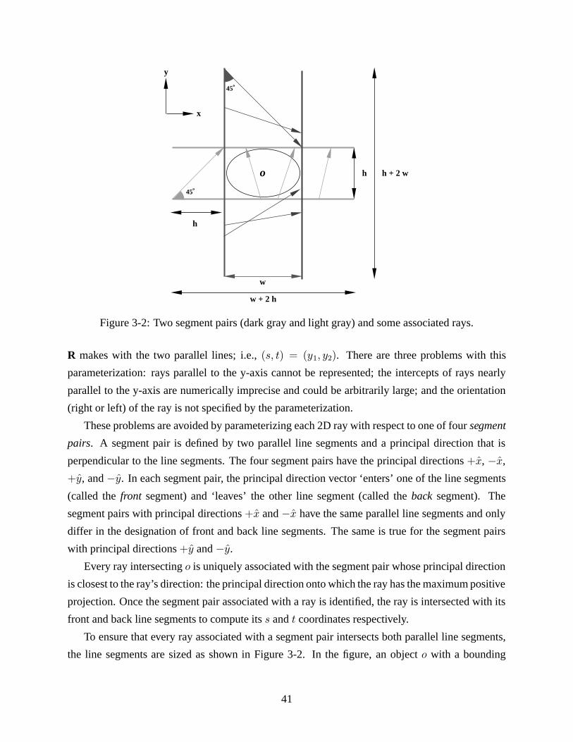
h

w

w + 2 h

h + 2 w

45o

45o

h

o

y

x

Figure 3-2: Two segment pairs (dark gray and light gray) and some associated rays.

R makes with the two parallel lines; i.e., (s, t) = (y1, y2). There are three problems with this

parameterization: rays parallel to the y-axis cannot be represented; the intercepts of rays nearly

parallel to the y-axis are numerically imprecise and could be arbitrarily large; and the orientation

(right or left) of the ray is not specified by the parameterization.

These problems are avoided by parameterizing each 2D ray with respect to one of four segment

pairs. A segment pair is defined by two parallel line segments and a principal direction that is

perpendicular to the line segments. The four segment pairs have the principal directions +x, −x,

+y, and −y. In each segment pair, the principal direction vector ‘enters’ one of the line segments

(called the front segment) and ‘leaves’ the other line segment (called the back segment). The

segment pairs with principal directions +x and −x have the same parallel line segments and only

differ in the designation of front and back line segments. The same is true for the segment pairs

with principal directions +y and −y.

Every ray intersecting o is uniquely associated with the segment pair whose principal direction

is closest to the ray’s direction: the principal direction onto which the ray has the maximum positive

projection. Once the segment pair associated with a ray is identified, the ray is intersected with its

front and back line segments to compute its s and t coordinates respectively.

To ensure that every ray associated with a segment pair intersects both parallel line segments,

the line segments are sized as shown in Figure 3-2. In the figure, an object o with a bounding

41

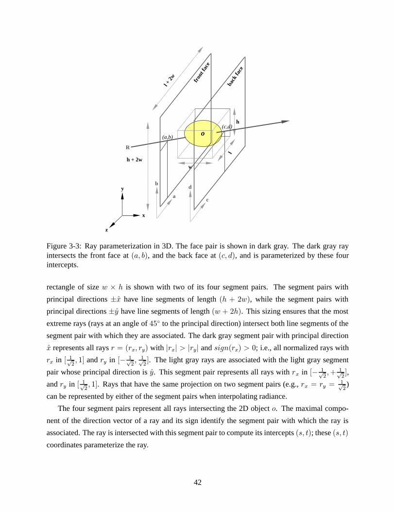
h + 2wl +

2w

w

h

l

(a,b)

(c,d)o

b

a

d

c

y

x

z

front

face

back

face

R

Figure 3-3: Ray parameterization in 3D. The face pair is shown in dark gray. The dark gray rayintersects the front face at (a, b), and the back face at (c, d), and is parameterized by these fourintercepts.

rectangle of size w × h is shown with two of its four segment pairs. The segment pairs with

principal directions ±x have line segments of length (h + 2w), while the segment pairs with

principal directions ±y have line segments of length (w + 2h). This sizing ensures that the most

extreme rays (rays at an angle of 45◦ to the principal direction) intersect both line segments of the

segment pair with which they are associated. The dark gray segment pair with principal direction

x represents all rays r = (rx, ry) with |rx| > |ry| and sign(rx) > 0; i.e., all normalized rays with

rx in [ 1√2, 1] and ry in [− 1√

2, 1√2]. The light gray rays are associated with the light gray segment

pair whose principal direction is y. This segment pair represents all rays with rx in [− 1√2,+ 1√

2],

and ry in [ 1√2, 1]. Rays that have the same projection on two segment pairs (e.g., rx = ry =

1√2)

can be represented by either of the segment pairs when interpolating radiance.

The four segment pairs represent all rays intersecting the 2D object o. The maximal compo-

nent of the direction vector of a ray and its sign identify the segment pair with which the ray is

associated. The ray is intersected with this segment pair to compute its intercepts (s, t); these (s, t)

coordinates parameterize the ray.

42

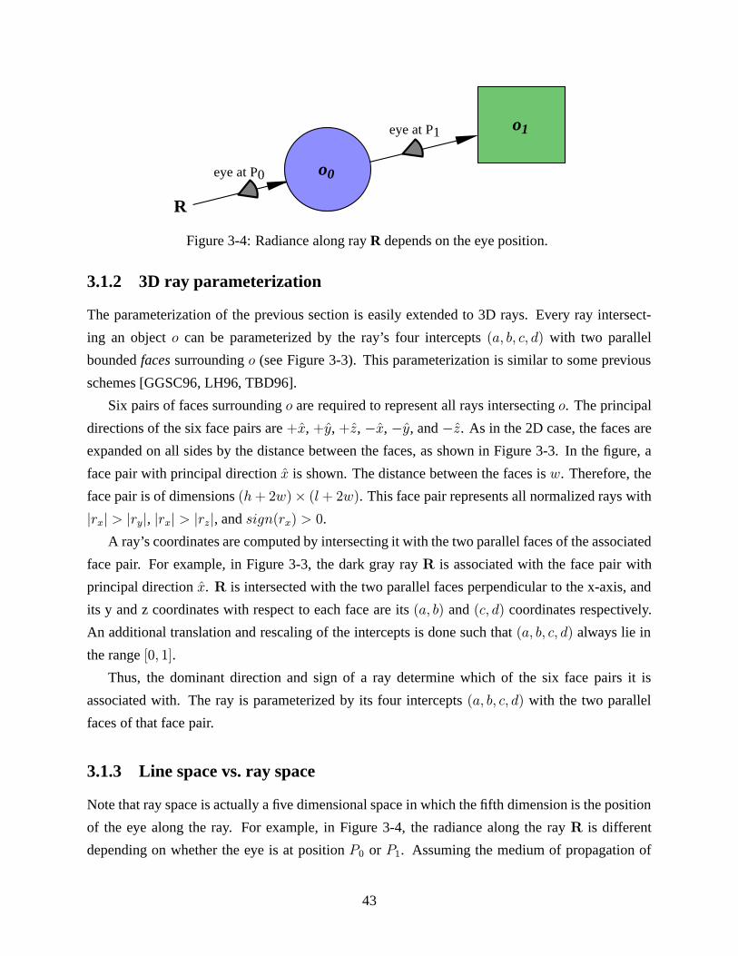
R

eye at P0

eye at P1

o0

o1

Figure 3-4: Radiance along ray R depends on the eye position.

3.1.2 3D ray parameterization

The parameterization of the previous section is easily extended to 3D rays. Every ray intersect-

ing an object o can be parameterized by the ray’s four intercepts (a, b, c, d) with two parallel

bounded facessurrounding o (see Figure 3-3). This parameterization is similar to some previous

schemes [GGSC96, LH96, TBD96].

Six pairs of faces surrounding o are required to represent all rays intersecting o. The principal

directions of the six face pairs are +x, +y, +z, −x, −y, and −z. As in the 2D case, the faces are

expanded on all sides by the distance between the faces, as shown in Figure 3-3. In the figure, a

face pair with principal direction x is shown. The distance between the faces is w. Therefore, the

face pair is of dimensions (h+ 2w)× (l + 2w). This face pair represents all normalized rays with

|rx| > |ry|, |rx| > |rz|, and sign(rx) > 0.

A ray’s coordinates are computed by intersecting it with the two parallel faces of the associated

face pair. For example, in Figure 3-3, the dark gray ray R is associated with the face pair with

principal direction x. R is intersected with the two parallel faces perpendicular to the x-axis, and

its y and z coordinates with respect to each face are its (a, b) and (c, d) coordinates respectively.

An additional translation and rescaling of the intercepts is done such that (a, b, c, d) always lie in

the range [0, 1].

Thus, the dominant direction and sign of a ray determine which of the six face pairs it is

associated with. The ray is parameterized by its four intercepts (a, b, c, d) with the two parallel

faces of that face pair.

3.1.3 Line space vs. ray space

Note that ray space is actually a five dimensional space in which the fifth dimension is the position

of the eye along the ray. For example, in Figure 3-4, the radiance along the ray R is different

depending on whether the eye is at position P0 or P1. Assuming the medium of propagation of

43

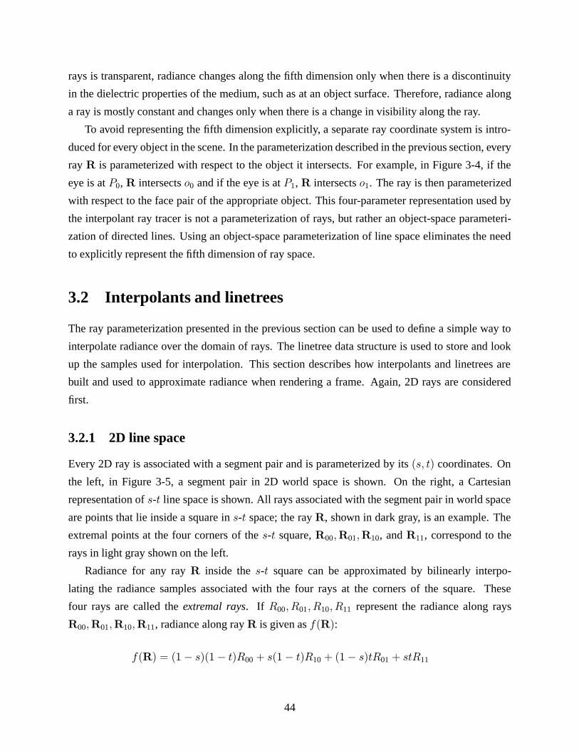
rays is transparent, radiance changes along the fifth dimension only when there is a discontinuity

in the dielectric properties of the medium, such as at an object surface. Therefore, radiance along

a ray is mostly constant and changes only when there is a change in visibility along the ray.

To avoid representing the fifth dimension explicitly, a separate ray coordinate system is intro-

duced for every object in the scene. In the parameterization described in the previous section, every

ray R is parameterized with respect to the object it intersects. For example, in Figure 3-4, if the

eye is at P0, R intersects o0 and if the eye is at P1, R intersects o1. The ray is then parameterized

with respect to the face pair of the appropriate object. This four-parameter representation used by

the interpolant ray tracer is not a parameterization of rays, but rather an object-space parameteri-

zation of directed lines. Using an object-space parameterization of line space eliminates the need

to explicitly represent the fifth dimension of ray space.

3.2 Interpolants and linetrees

The ray parameterization presented in the previous section can be used to define a simple way to

interpolate radiance over the domain of rays. The linetree data structure is used to store and look

up the samples used for interpolation. This section describes how interpolants and linetrees are

built and used to approximate radiance when rendering a frame. Again, 2D rays are considered

first.

3.2.1 2D line space

Every 2D ray is associated with a segment pair and is parameterized by its (s, t) coordinates. On

the left, in Figure 3-5, a segment pair in 2D world space is shown. On the right, a Cartesian

representation of s-t line space is shown. All rays associated with the segment pair in world space

are points that lie inside a square in s-t space; the ray R, shown in dark gray, is an example. The

extremal points at the four corners of the s-t square, R00,R01,R10, and R11, correspond to the

rays in light gray shown on the left.

Radiance for any ray R inside the s-t square can be approximated by bilinearly interpo-

lating the radiance samples associated with the four rays at the corners of the square. These

four rays are called the extremal rays. If R00, R01, R10, R11 represent the radiance along rays

R00,R01,R10,R11, radiance along rayR is given as f(R):

f(R) = (1− s)(1− t)R00 + s(1− t)R10 + (1− s)tR01 + stR11

44

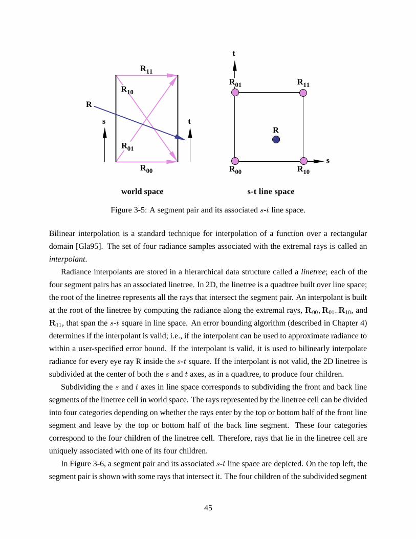
R

s t

world space

R00

R11

s-t line space

s

t

R11

R00

R01

R10

R

R10

R01

Figure 3-5: A segment pair and its associated s-t line space.

Bilinear interpolation is a standard technique for interpolation of a function over a rectangular

domain [Gla95]. The set of four radiance samples associated with the extremal rays is called an

interpolant.

Radiance interpolants are stored in a hierarchical data structure called a linetree; each of the

four segment pairs has an associated linetree. In 2D, the linetree is a quadtree built over line space;

the root of the linetree represents all the rays that intersect the segment pair. An interpolant is built

at the root of the linetree by computing the radiance along the extremal rays, R00,R01,R10, and

R11, that span the s-t square in line space. An error bounding algorithm (described in Chapter 4)

determines if the interpolant is valid; i.e., if the interpolant can be used to approximate radiance to

within a user-specified error bound. If the interpolant is valid, it is used to bilinearly interpolate

radiance for every eye ray R inside the s-t square. If the interpolant is not valid, the 2D linetree is

subdivided at the center of both the s and t axes, as in a quadtree, to produce four children.

Subdividing the s and t axes in line space corresponds to subdividing the front and back line

segments of the linetree cell in world space. The rays represented by the linetree cell can be divided

into four categories depending on whether the rays enter by the top or bottom half of the front line

segment and leave by the top or bottom half of the back line segment. These four categories

correspond to the four children of the linetree cell. Therefore, rays that lie in the linetree cell are

uniquely associated with one of its four children.

In Figure 3-6, a segment pair and its associated s-t line space are depicted. On the top left, the

segment pair is shown with some rays that intersect it. The four children of the subdivided segment

45

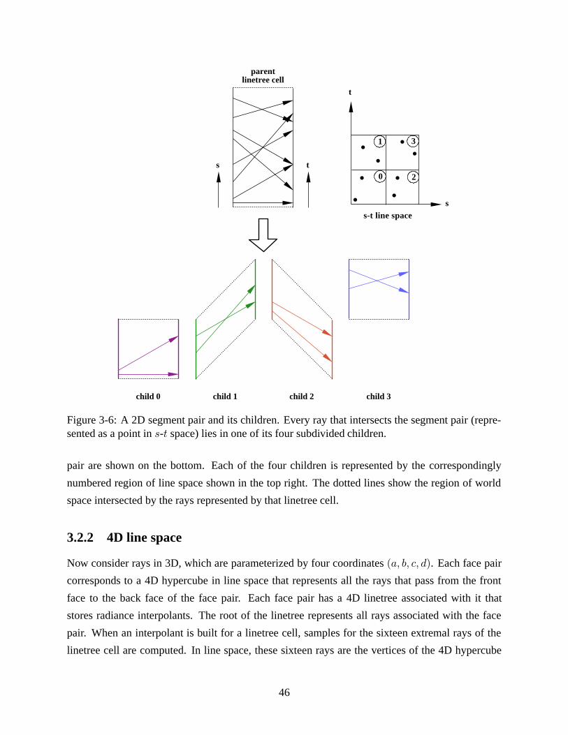
child 0 child 1 child 3child 2

s t

parentlinetree cell

s-t line spaces

t

0

1

2

3

Figure 3-6: A 2D segment pair and its children. Every ray that intersects the segment pair (repre-sented as a point in s-t space) lies in one of its four subdivided children.

pair are shown on the bottom. Each of the four children is represented by the correspondingly

numbered region of line space shown in the top right. The dotted lines show the region of world

space intersected by the rays represented by that linetree cell.

3.2.2 4D line space

Now consider rays in 3D, which are parameterized by four coordinates (a, b, c, d). Each face pair

corresponds to a 4D hypercube in line space that represents all the rays that pass from the front

face to the back face of the face pair. Each face pair has a 4D linetree associated with it that

stores radiance interpolants. The root of the linetree represents all rays associated with the face

pair. When an interpolant is built for a linetree cell, samples for the sixteen extremal rays of the

linetree cell are computed. In line space, these sixteen rays are the vertices of the 4D hypercube

46

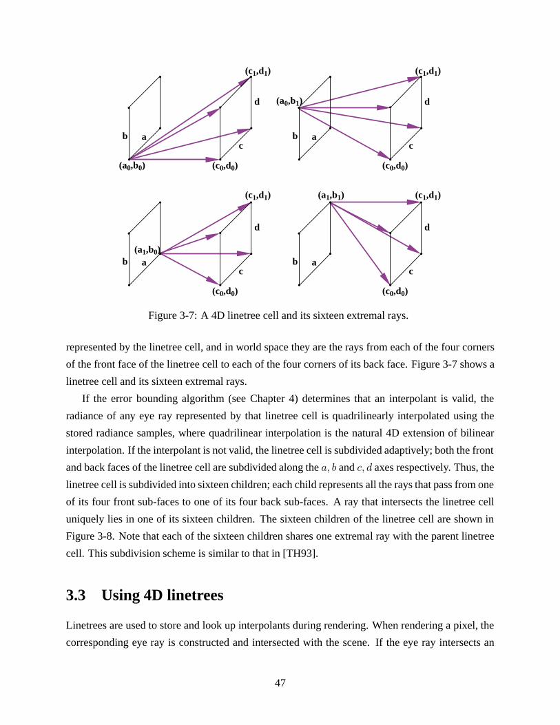
(a1,b0)

(a0,b0)

(c1,d1)

(a0,b1)

(a1,b1)

b

b b

b

(c1,d1)

(c0,d0)

d

c

(c1,d1)

(c0,d0)

d

c

(c0,d0)

d

c

(c1,d1)

(c0,d0)

d

ca

a a

a

Figure 3-7: A 4D linetree cell and its sixteen extremal rays.

represented by the linetree cell, and in world space they are the rays from each of the four corners

of the front face of the linetree cell to each of the four corners of its back face. Figure 3-7 shows a

linetree cell and its sixteen extremal rays.

If the error bounding algorithm (see Chapter 4) determines that an interpolant is valid, the

radiance of any eye ray represented by that linetree cell is quadrilinearly interpolated using the

stored radiance samples, where quadrilinear interpolation is the natural 4D extension of bilinear

interpolation. If the interpolant is not valid, the linetree cell is subdivided adaptively; both the front

and back faces of the linetree cell are subdivided along the a, b and c, d axes respectively. Thus, the

linetree cell is subdivided into sixteen children; each child represents all the rays that pass from one

of its four front sub-faces to one of its four back sub-faces. A ray that intersects the linetree cell

uniquely lies in one of its sixteen children. The sixteen children of the linetree cell are shown in

Figure 3-8. Note that each of the sixteen children shares one extremal ray with the parent linetree

cell. This subdivision scheme is similar to that in [TH93].

3.3 Using 4D linetrees

Linetrees are used to store and look up interpolants during rendering. When rendering a pixel, the

corresponding eye ray is constructed and intersected with the scene. If the eye ray intersects an

47

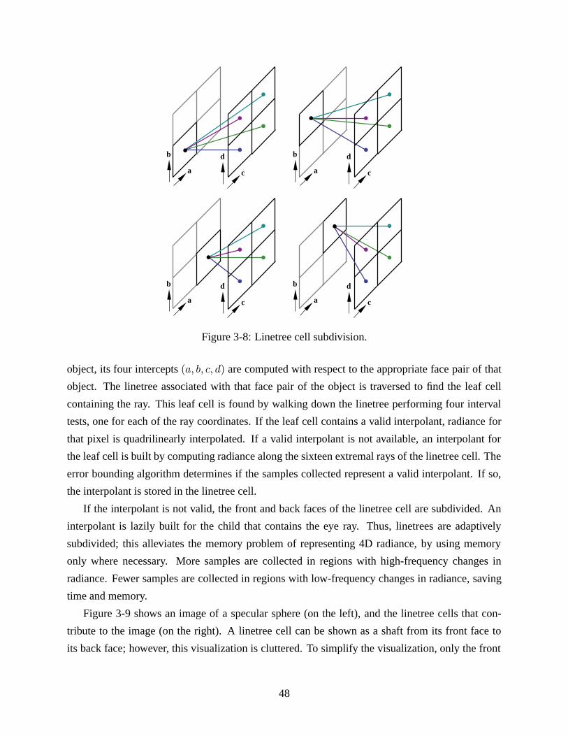
a

b

c

d

a

b

c

d

a

b

c

d

a

b

c

d

Figure 3-8: Linetree cell subdivision.

object, its four intercepts (a, b, c, d) are computed with respect to the appropriate face pair of that

object. The linetree associated with that face pair of the object is traversed to find the leaf cell

containing the ray. This leaf cell is found by walking down the linetree performing four interval

tests, one for each of the ray coordinates. If the leaf cell contains a valid interpolant, radiance for

that pixel is quadrilinearly interpolated. If a valid interpolant is not available, an interpolant for

the leaf cell is built by computing radiance along the sixteen extremal rays of the linetree cell. The

error bounding algorithm determines if the samples collected represent a valid interpolant. If so,

the interpolant is stored in the linetree cell.

If the interpolant is not valid, the front and back faces of the linetree cell are subdivided. An

interpolant is lazily built for the child that contains the eye ray. Thus, linetrees are adaptively

subdivided; this alleviates the memory problem of representing 4D radiance, by using memory

only where necessary. More samples are collected in regions with high-frequency changes in

radiance. Fewer samples are collected in regions with low-frequency changes in radiance, saving

time and memory.

Figure 3-9 shows an image of a specular sphere (on the left), and the linetree cells that con-

tribute to the image (on the right). A linetree cell can be shown as a shaft from its front face to

its back face; however, this visualization is cluttered. To simplify the visualization, only the front

48

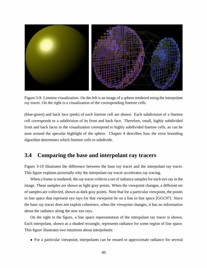
Figure 3-9: Linetree visualization. On the left is an image of a sphere rendered using the interpolantray tracer. On the right is a visualization of the corresponding linetree cells.

(blue-green) and back face (pink) of each linetree cell are shown. Each subdivision of a linetree

cell corresponds to a subdivision of its front and back face. Therefore, small, highly subdivided

front and back faces in the visualization correspond to highly subdivided linetree cells, as can be

seen around the specular highlight of the sphere. Chapter 4 describes how the error bounding

algorithm determines which linetree cells to subdivide.

3.4 Comparing the base and interpolant ray tracers

Figure 3-10 illustrates the difference between the base ray tracer and the interpolant ray tracer.

This figure explains pictorially why the interpolant ray tracer accelerates ray tracing.

When a frame is rendered, the ray tracer collects a set of radiance samples for each eye ray in the

image. These samples are shown as light gray points. When the viewpoint changes, a different set

of samples are collected, shown as dark gray points. Note that for a particular viewpoint, the points

in line space that represent eye rays for that viewpoint lie on a line in line space [GGC97]. Since

the base ray tracer does not exploit coherence, when the viewpoint changes, it has no information

about the radiance along the new eye rays.

On the right in the figure, a line space representation of the interpolant ray tracer is shown.

Each interpolant, shown as a shaded rectangle, represents radiance for some region of line space.

This figure illustrates two intuitions about interpolants:

• For a particular viewpoint, interpolants can be reused to approximate radiance for several

49

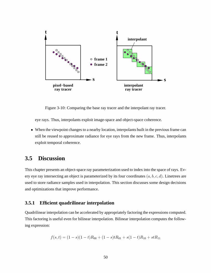
s

t

pixel−basedray tracer

s

t

interpolantray tracer

frame 1frame 2

interpolant

Figure 3-10: Comparing the base ray tracer and the interpolant ray tracer.

eye rays. Thus, interpolants exploit image-space and object-space coherence.

• When the viewpoint changes to a nearby location, interpolants built in the previous frame can

still be reused to approximate radiance for eye rays from the new frame. Thus, interpolants

exploit temporal coherence.

3.5 Discussion

This chapter presents an object-space ray parameterization used to index into the space of rays. Ev-

ery eye ray intersecting an object is parameterized by its four coordinates (a, b, c, d). Linetrees are

used to store radiance samples used in interpolation. This section discusses some design decisions

and optimizations that improve performance.

3.5.1 Efficient quadrilinear interpolation

Quadrilinear interpolation can be accelerated by appropriately factoring the expressions computed.

This factoring is useful even for bilinear interpolation. Bilinear interpolation computes the follow-

ing expression:

f(s, t) = (1− s)(1− t)R00 + (1− s)tR01 + s(1− t)R10 + stR11

50

Evaluating this expression sequentially, as written, requires eight multiplications and five additions,

assuming that the values of (1−s) and (1−t) are computed only once. It is well-known that bilinear

interpolation can be computed faster using the following factorization [Pra91]:

f(s, t) = (1− s) [(1− t)R00 + tR01] + s [(1− t)R10 + tR11]

This formula can be expressed in terms of a linear interpolation function L:

L(x, y0, y1) = (1− x)y0 + xy1 = y0 + x(y1 − y0)

The function L can be computed using one multiplication and two additions using the rightmost

expression. The bilinear interpolation can be expressed using L as follows:

f(s, t) = (1− s)L(t, R00, R01) + sL(t, R10, R11)

= L(s, L(t, R00, R01), L(t, R10, R11))

The function f is computed with three applications of L, so the total cost is three multiplica-

tions and six additions. Multiplication is usually slower than addition, so this computation is an

improvement. This factoring is even more effective for quadrilinear interpolation, where the num-

ber of multiplications is decreased from 64 to 15, while the number of additions is increased from

19 to 30. In general, for interpolation in n dimensions, this factoring allows us to trade (n−1)2n+1

multiplications for 2n − n− 1 additions, which is always a speedup if multiplication is at least as

slow as addition.

3.5.2 Adaptive linetree subdivision

A linetree cell is subdivided if the sixteen extremal samples associated with the cell do not ap-

proximate the radiance function over the cell acceptably. When a linetree cell is subdivided, all

four axes of the cell are subdivided. If no information is available about the form of the radiance

function that the cell represents, this greedy subdivision makes sense. However, if information

about how the radiance function varies is available, this information can be used to drive adaptive

subdivision. This concept is reminiscent of the use of information about the distribution of objects

in a 3D scene to build optimal spatial subdivisions of the scene [FI85, Jan86, Gla89].

The subdivision algorithm presented earlier in this chapter greedily splits a linetree cell into

sixteen children. The interpolant ray tracer implements a 4-way split algorithm that splits only two

of the axes (a, c) or (b, d) at a time; each linetree cell is subdivided into four children. The pair of

51

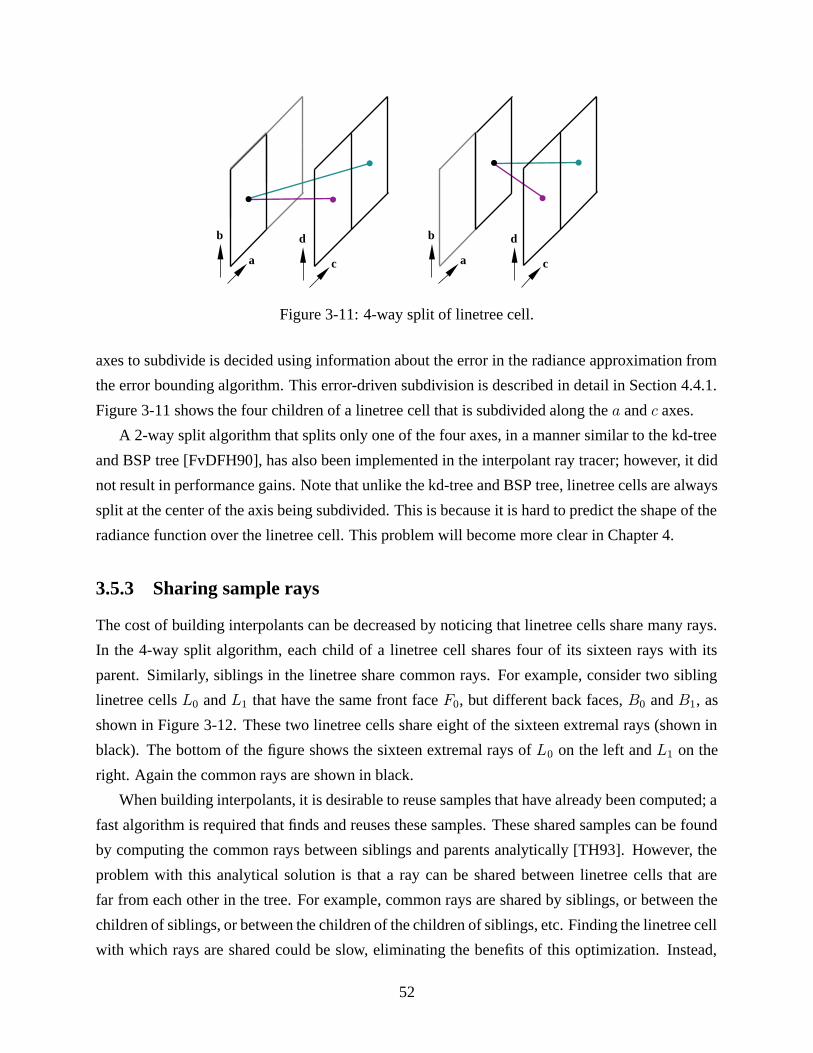
a

b

c

d

a

b

c

d

Figure 3-11: 4-way split of linetree cell.

axes to subdivide is decided using information about the error in the radiance approximation from

the error bounding algorithm. This error-driven subdivision is described in detail in Section 4.4.1.

Figure 3-11 shows the four children of a linetree cell that is subdivided along the a and c axes.

A 2-way split algorithm that splits only one of the four axes, in a manner similar to the kd-tree

and BSP tree [FvDFH90], has also been implemented in the interpolant ray tracer; however, it did

not result in performance gains. Note that unlike the kd-tree and BSP tree, linetree cells are always

split at the center of the axis being subdivided. This is because it is hard to predict the shape of the

radiance function over the linetree cell. This problem will become more clear in Chapter 4.

3.5.3 Sharing sample rays

The cost of building interpolants can be decreased by noticing that linetree cells share many rays.

In the 4-way split algorithm, each child of a linetree cell shares four of its sixteen rays with its

parent. Similarly, siblings in the linetree share common rays. For example, consider two sibling

linetree cells L0 and L1 that have the same front face F0, but different back faces, B0 and B1, as

shown in Figure 3-12. These two linetree cells share eight of the sixteen extremal rays (shown in

black). The bottom of the figure shows the sixteen extremal rays of L0 on the left and L1 on the

right. Again the common rays are shown in black.

When building interpolants, it is desirable to reuse samples that have already been computed; a

fast algorithm is required that finds and reuses these samples. These shared samples can be found

by computing the common rays between siblings and parents analytically [TH93]. However, the

problem with this analytical solution is that a ray can be shared between linetree cells that are

far from each other in the tree. For example, common rays are shared by siblings, or between the

children of siblings, or between the children of the children of siblings, etc. Finding the linetree cell

with which rays are shared could be slow, eliminating the benefits of this optimization. Instead,

52

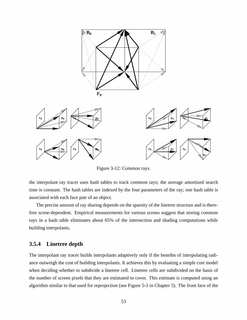
B0

F0

B1

F0 B0

F0 B0 F0

F0

B0

B0 F0 B1

F0 B1 F0

F0

B1

B1

Figure 3-12: Common rays.

the interpolant ray tracer uses hash tables to track common rays; the average amortized search

time is constant. The hash tables are indexed by the four parameters of the ray; one hash table is

associated with each face pair of an object.

The precise amount of ray sharing depends on the sparsity of the linetree structure and is there-

fore scene-dependent. Empirical measurements for various scenes suggest that storing common

rays in a hash table eliminates about 65% of the intersection and shading computations while

building interpolants.

3.5.4 Linetree depth

The interpolant ray tracer builds interpolants adaptively only if the benefits of interpolating radi-

ance outweigh the cost of building interpolants. It achieves this by evaluating a simple cost model

when deciding whether to subdivide a linetree cell. Linetree cells are subdivided on the basis of

the number of screen pixels that they are estimated to cover. This estimate is computed using an

algorithm similar to that used for reprojection (see Figure 5-3 in Chapter 5). The front face of the

53

linetree cell is projected onto its back plane, and clipped against its back face. When this clipped

back face is projected on the image plane, its area is a good estimate of the number of pixels cov-

ered by the linetree cell for that frame. Thus, when the observer zooms in on an object, interpolants

for that object are built to a greater resolution if required by the error bounding algorithm; if an

observer is far away from an object, the interpolants are coarse, saving memory. This cost model

ensures that the cost of building interpolants is amortized over several pixels. The best results are

found empirically to occur when an interpolant is built only if it covers at least twelve pixels on

the image plane. It makes sense that this setting delivers the best performance because building

an interpolant is roughly twelve times more expensive than shooting a single ray. This follows

because four of the sixteen samples associated with the interpolant have already been computed

for its parent linetree cell and are reused, as explained in the previous section.

3.5.5 Linetree lookup cache

Ray space and screen space coherence are exploited by the following optimization. For every eye

ray in the image, the algorithm finds the object intersected by the ray, and then walks down the

appropriate linetree of the object, starting at the root of the linetree. Linetrees are subdivided to a

depth of 8 to 16 for typical scenes; traversing these linetrees from the root to the leaf takes time.

However, because of screen space and ray space coherence, a linetree leaf cell typically con-

tributes to the radiance of multiple pixels in an image. Therefore, a linetree cache per object can be

maintained that stores the linetree leaf cell last used to satisfy a query for this object. As the frame

is rendered, for each new ray R, this cache is checked to see if R lies in the cached leaf linetree

cell. If it does, no traversal of the linetree from the root is required. This cache is effective: its hit

rate is 70-75%. As an additional optimization, when the cache lookup fails, the system walks up

from the cached linetree cell to the linetree cell of the closest ancestor that includes R and then

walks down from that ancestor. Since there is ray space coherence, the closest ancestor is typically

close to the cached leaf. This walk up and down the tree is faster than walking down from the root.

Eliminating the traversal from the root to the leaf of a linetree decreases the average time to find a

linetree cell from 9µs to 3.5µs on a 194MHz MIPS R10000 processor.

3.5.6 Alternative data structures

This section considers alternatives for storing and interpolating radiance samples, and their ex-

pected impact on performance. Building interpolants is expensive; it would be beneficial to use a

smaller number of samples to interpolate radiance. In order to interpolate a function over a region

54

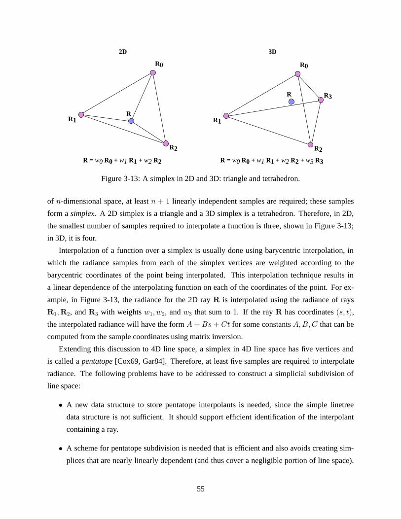
R = w0 R0 + w1 R1 + w2 R2 + w3 R3

3D

R0

R2

R R3

R1

R = w0 R0 + w1 R1 + w2 R2

2D

R0

R2

R1R

Figure 3-13: A simplex in 2D and 3D: triangle and tetrahedron.

of n-dimensional space, at least n + 1 linearly independent samples are required; these samples

form a simplex. A 2D simplex is a triangle and a 3D simplex is a tetrahedron. Therefore, in 2D,

the smallest number of samples required to interpolate a function is three, shown in Figure 3-13;

in 3D, it is four.

Interpolation of a function over a simplex is usually done using barycentric interpolation, in

which the radiance samples from each of the simplex vertices are weighted according to the

barycentric coordinates of the point being interpolated. This interpolation technique results in

a linear dependence of the interpolating function on each of the coordinates of the point. For ex-

ample, in Figure 3-13, the radiance for the 2D ray R is interpolated using the radiance of rays

R1,R2, and R3 with weights w1, w2, and w3 that sum to 1. If the ray R has coordinates (s, t),

the interpolated radiance will have the form A +Bs + Ct for some constants A,B,C that can be

computed from the sample coordinates using matrix inversion.

Extending this discussion to 4D line space, a simplex in 4D line space has five vertices and

is called a pentatope[Cox69, Gar84]. Therefore, at least five samples are required to interpolate

radiance. The following problems have to be addressed to construct a simplicial subdivision of

line space:

• A new data structure to store pentatope interpolants is needed, since the simple linetree

data structure is not sufficient. It should support efficient identification of the interpolant

containing a ray.

• A scheme for pentatope subdivision is needed that is efficient and also avoids creating sim-

plices that are nearly linearly dependent (and thus cover a negligible portion of line space).

55

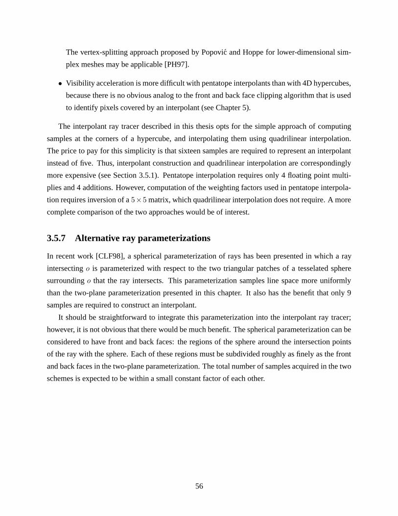
The vertex-splitting approach proposed by Popovic and Hoppe for lower-dimensional sim-

plex meshes may be applicable [PH97].

• Visibility acceleration is more difficult with pentatope interpolants than with 4D hypercubes,

because there is no obvious analog to the front and back face clipping algorithm that is used

to identify pixels covered by an interpolant (see Chapter 5).

The interpolant ray tracer described in this thesis opts for the simple approach of computing

samples at the corners of a hypercube, and interpolating them using quadrilinear interpolation.

The price to pay for this simplicity is that sixteen samples are required to represent an interpolant

instead of five. Thus, interpolant construction and quadrilinear interpolation are correspondingly

more expensive (see Section 3.5.1). Pentatope interpolation requires only 4 floating point multi-

plies and 4 additions. However, computation of the weighting factors used in pentatope interpola-

tion requires inversion of a 5×5 matrix, which quadrilinear interpolation does not require. A more

complete comparison of the two approaches would be of interest.

3.5.7 Alternative ray parameterizations

In recent work [CLF98], a spherical parameterization of rays has been presented in which a ray

intersecting o is parameterized with respect to the two triangular patches of a tesselated sphere

surrounding o that the ray intersects. This parameterization samples line space more uniformly

than the two-plane parameterization presented in this chapter. It also has the benefit that only 9

samples are required to construct an interpolant.

It should be straightforward to integrate this parameterization into the interpolant ray tracer;

however, it is not obvious that there would be much benefit. The spherical parameterization can be

considered to have front and back faces: the regions of the sphere around the intersection points

of the ray with the sphere. Each of these regions must be subdivided roughly as finely as the front

and back faces in the two-plane parameterization. The total number of samples acquired in the two

schemes is expected to be within a small constant factor of each other.

56

Chapter 4

Error Bounds

The interpolant ray tracer samples radiance adaptively, collecting more samples where radiance

varies rapidly and fewer samples where radiance varies smoothly. To enable this adaptive division,

the system must determine how radiance changes over the domain of rays. This chapter presents

an error bounding algorithm that characterizes how radiance varies over line space and determines

whether each interpolant built approximates radiance well.

4.1 Overview

The error bounding algorithm described in this chapter is used to determine when an interpolant

is valid; an interpolant is valid if it can be used to interpolate radiance sufficiently well over the

associated linetree cell. For example, if radiance changes discontinuously over a linetree cell,

interpolation across the cell would result in the blurring of the sharp discontinuous edge; the cor-

responding interpolant is therefore invalid. When the error bounding algorithm determines that an

interpolant is invalid, the ray tracer subdivides the linetree cell associated with the interpolant as

described in Chapter 3.

In providing this error bounding algorithm, this thesis makes several contributions to the prob-

lem of bounding radiance interpolation error:

• It categorizes interpolation error into two major classes: error due to discontinuities and error

due to non-linear radiance variations.

• It describes the various ways in which radiance discontinuities can cause interpolation error

and presents geometric techniques to conservatively identify each type of radiance disconti-

nuity.

57

• It introduces a novel use of a multi-variate generalization of interval arithmetic to conserva-

tively bound interpolation error arising from non-linear variations in radiance.

Together, these techniques provide the first complete, conservative characterization of interpolation

error; importantly for the acceleration of ray tracing, the error bounds derived are accurate and can

be computed efficiently.

4.1.1 Interpolant validation

First, we must consider how interpolation error can arise. The interpolant ray tracer uses quadri-

linear interpolation to approximate radiance for all rays represented by a linetree cell. Quadrilinear

interpolation is accurate as long as radiance within the cell has a linear dependence on the line

space coordinates (a, b, c, d). Interpolation error arises only if there is a non-linear variation in the

radiance over the cell.

Interpolation error can arise in two ways:

• Interpolation over a radiance discontinuity (for example, due to shadows, occluding objects

or total internal reflection).

• Interpolation over regions of line space in which radiance varies non-linearly (for example,

due to diffuse or specular peaks).

Discontinuities are treated as a special case because the human eye is sensitive to discontinuous

changes in radiance [Gla95]. Therefore, interpolating across a radiance discontinuity is perceived

as erroneous by the human eye, even if the resultant interpolation error is less than ε.

Thus, the error bounding algorithm receives as input the sixteen radiance samples of the ex-

tremal rays of a linetree cell, and determines if the interpolant is valid by answering the following

two questions conservatively:

1. Does radiance change discontinuously anywherein the region of line space represented by

the linetree cell?

2. If radiance does not change discontinuously, is the quadrilinearly interpolated radiance within

ε of the radiance computed by the base ray tracer for everyray represented by that linetree

cell?

If either answer is no, the interpolant is invalid, and the linetree cell is subdivided.

This chapter presents techniques to identify both discontinuities and non-linearities. Together,

these techniques completely specify the error bounding algorithm.

58

4.1.2 Assumptions and limitations

The error bounding algorithm is based on certain assumptions about the scene being rendered and

the rendering model. These assumptions affect the difficulty of bounding error in various ways.

The assumptions are as follows:

1. The scene is composed of convex objects: spheres, cubes, polygons, cylinders and cones

and the CSG union and intersection of these primitives [Rot82] are supported. This assump-

tion simplifies the detection of certains kinds of discontinuities; for example, discontinuities

arising from shadow edges.

2. The base ray tracer implements a classical Whitted ray tracer, sampling the reflected and re-

fracted directions. The local shading model used is the Ward isotropic shading model [War92].

3. Textures for the diffuse color of a surface are supported.

4. Lights are assumed to be either infinite light sources, local light sources, or spotlights.

Each of these assumptions imposes limitations on the system; some of these limitations are

easily addressed, while others are areas for future research. Note that the interpolation mechanism

described in Chapter 3 is applicable to a broader range of scenes and rendering models; only

the error bounding algorithm, described in this chapter, is tied closely to this set of assumptions.

Section 4.5 discusses extensions to address these limitations.

The rest of this chapter is organized as follows. Section 4.2 presents a taxonomy of the different

types of radiance discontinuities and shows how to detect and avoid interpolation over each type

of discontinuity. Section 4.3 describes how interpolation error can arise from non-linear variations

in radiance and introduces the use of multi-variate linear interval arithmetic to bound interpolation

error over non-linear radiance variations. Section 4.4 presents various optimizations. Section 4.5

discusses extensions to the error bounding algorithm to support more complex scenes and render-

ing models. Finally, Section 4.6 discusses alternatives to bounding error.

4.2 Radiance discontinuities

Radiance discontinuities arise because the scene is composed of multiple objects that occlude and

cast shadows on each other. First, this section presents the invariant that should be maintained to

ensure that an interpolant does not include any discontinuities. Then, a taxonomy of the different

kinds of radiance discontinuities is presented. Finally, geometric techniques to detect each possible

discontinuity are presented.

59

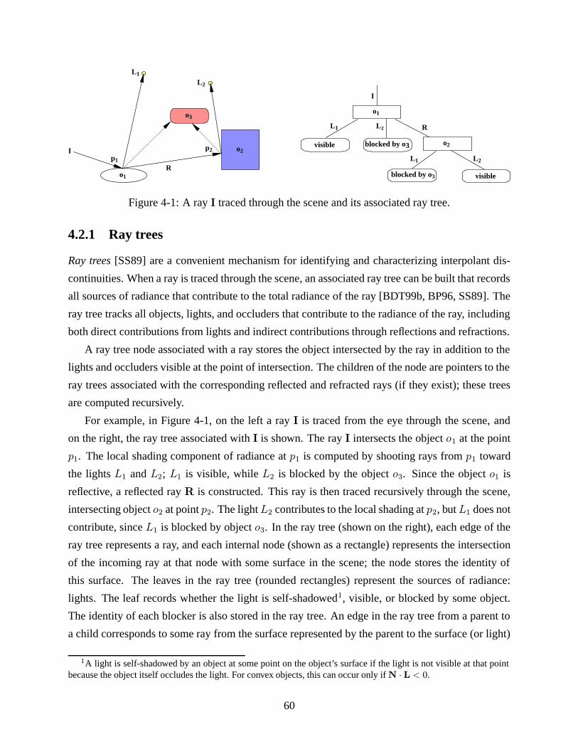
I

R

o1

o2

L2

visible

L1

L1 L2

visible blocked by o3

blocked by o3

I

R

L1

o1

o2

o3

L2

p1

p2

Figure 4-1: A ray I traced through the scene and its associated ray tree.

4.2.1 Ray trees

Ray trees[SS89] are a convenient mechanism for identifying and characterizing interpolant dis-

continuities. When a ray is traced through the scene, an associated ray tree can be built that records

all sources of radiance that contribute to the total radiance of the ray [BDT99b, BP96, SS89]. The

ray tree tracks all objects, lights, and occluders that contribute to the radiance of the ray, including

both direct contributions from lights and indirect contributions through reflections and refractions.

A ray tree node associated with a ray stores the object intersected by the ray in addition to the

lights and occluders visible at the point of intersection. The children of the node are pointers to the

ray trees associated with the corresponding reflected and refracted rays (if they exist); these trees

are computed recursively.

For example, in Figure 4-1, on the left a ray I is traced from the eye through the scene, and

on the right, the ray tree associated with I is shown. The ray I intersects the object o1 at the point

p1. The local shading component of radiance at p1 is computed by shooting rays from p1 toward

the lights L1 and L2; L1 is visible, while L2 is blocked by the object o3. Since the object o1 is

reflective, a reflected ray R is constructed. This ray is then traced recursively through the scene,

intersecting object o2 at point p2. The light L2 contributes to the local shading at p2, but L1 does not

contribute, since L1 is blocked by object o3. In the ray tree (shown on the right), each edge of the

ray tree represents a ray, and each internal node (shown as a rectangle) represents the intersection

of the incoming ray at that node with some surface in the scene; the node stores the identity of

this surface. The leaves in the ray tree (rounded rectangles) represent the sources of radiance:

lights. The leaf records whether the light is self-shadowed1, visible, or blocked by some object.

The identity of each blocker is also stored in the ray tree. An edge in the ray tree from a parent to

a child corresponds to some ray from the surface represented by the parent to the surface (or light)

1A light is self-shadowed by an object at some point on the object’s surface if the light is not visible at that pointbecause the object itself occludes the light. For convex objects, this can occur only ifN · L < 0.

60

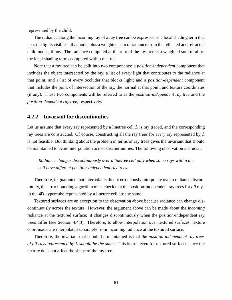
represented by the child.

The radiance along the incoming ray of a ray tree can be expressed as a local shading term that

uses the lights visible at that node, plus a weighted sum of radiance from the reflected and refracted

child nodes, if any. The radiance computed at the root of the ray tree is a weighted sum of all of

the local shading terms computed within the tree.

Note that a ray tree can be split into two components: a position-independentcomponent that

includes the object intersected by the ray, a list of every light that contributes to the radiance at

that point, and a list of every occluder that blocks light; and a position-dependentcomponent

that includes the point of intersection of the ray, the normal at that point, and texture coordinates

(if any). These two components will be referred to as the position-independent ray treeand the

position-dependent ray tree, respectively.

4.2.2 Invariant for discontinuities

Let us assume that every ray represented by a linetree cell L is ray traced, and the corresponding

ray trees are constructed. Of course, constructing all the ray trees for everyray represented by L

is not feasible. But thinking about the problem in terms of ray trees gives the invariant that should

be maintained to avoid interpolation across discontinuities. The following observation is crucial:

Radiance changes discontinuously over a linetree cell only when some rays within the

cell have different position-independent ray trees.

Therefore, to guarantee that interpolants do not erroneously interpolate over a radiance discon-

tinuity, the error bounding algorithm must check that the position-independent ray trees for all rays

in the 4D hypercube represented by a linetree cell are the same.

Textured surfaces are an exception to the observation above because radiance can change dis-

continuously across the texture. However, the argument above can be made about the incoming

radiance at the textured surface: it changes discontinuously when the position-independent ray

trees differ (see Section 4.4.3). Therefore, to allow interpolation over textured surfaces, texture

coordinates are interpolated separately from incoming radiance at the textured surface.

Therefore, the invariant that should be maintained is that the position-independent ray trees

of all rays represented by L should be the same. This is true even for textured surfaces since the

texture does not affect the shape of the ray tree.

61

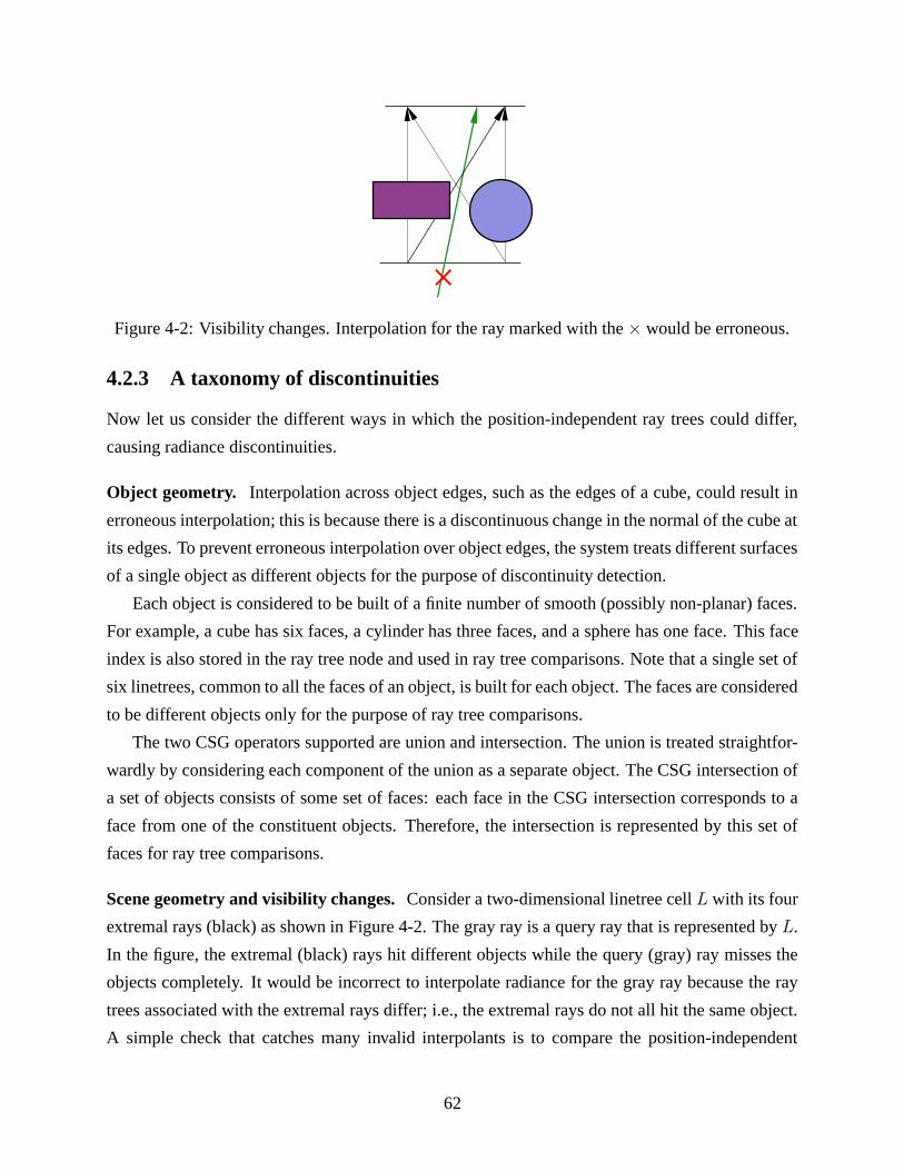
Figure 4-2: Visibility changes. Interpolation for the ray marked with the × would be erroneous.

4.2.3 A taxonomy of discontinuities

Now let us consider the different ways in which the position-independent ray trees could differ,

causing radiance discontinuities.

Object geometry. Interpolation across object edges, such as the edges of a cube, could result in

erroneous interpolation; this is because there is a discontinuous change in the normal of the cube at

its edges. To prevent erroneous interpolation over object edges, the system treats different surfaces

of a single object as different objects for the purpose of discontinuity detection.

Each object is considered to be built of a finite number of smooth (possibly non-planar) faces.

For example, a cube has six faces, a cylinder has three faces, and a sphere has one face. This face

index is also stored in the ray tree node and used in ray tree comparisons. Note that a single set of

six linetrees, common to all the faces of an object, is built for each object. The faces are considered

to be different objects only for the purpose of ray tree comparisons.

The two CSG operators supported are union and intersection. The union is treated straightfor-

wardly by considering each component of the union as a separate object. The CSG intersection of

a set of objects consists of some set of faces: each face in the CSG intersection corresponds to a

face from one of the constituent objects. Therefore, the intersection is represented by this set of

faces for ray tree comparisons.

Scene geometry and visibility changes. Consider a two-dimensional linetree cell L with its four

extremal rays (black) as shown in Figure 4-2. The gray ray is a query ray that is represented by L.

In the figure, the extremal (black) rays hit different objects while the query (gray) ray misses the

objects completely. It would be incorrect to interpolate radiance for the gray ray because the ray

trees associated with the extremal rays differ; i.e., the extremal rays do not all hit the same object.

A simple check that catches many invalid interpolants is to compare the position-independent

62

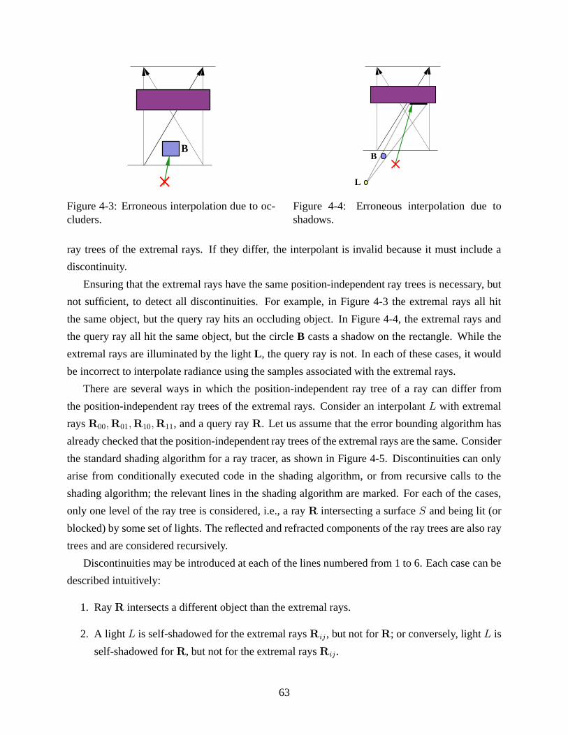
B

Figure 4-3: Erroneous interpolation due to oc-cluders.

L

B

Figure 4-4: Erroneous interpolation due toshadows.

ray trees of the extremal rays. If they differ, the interpolant is invalid because it must include a

discontinuity.

Ensuring that the extremal rays have the same position-independent ray trees is necessary, but

not sufficient, to detect all discontinuities. For example, in Figure 4-3 the extremal rays all hit

the same object, but the query ray hits an occluding object. In Figure 4-4, the extremal rays and

the query ray all hit the same object, but the circle B casts a shadow on the rectangle. While the

extremal rays are illuminated by the light L, the query ray is not. In each of these cases, it would

be incorrect to interpolate radiance using the samples associated with the extremal rays.

There are several ways in which the position-independent ray tree of a ray can differ from

the position-independent ray trees of the extremal rays. Consider an interpolant L with extremal

rays R00,R01,R10,R11, and a query ray R. Let us assume that the error bounding algorithm has

already checked that the position-independent ray trees of the extremal rays are the same. Consider

the standard shading algorithm for a ray tracer, as shown in Figure 4-5. Discontinuities can only

arise from conditionally executed code in the shading algorithm, or from recursive calls to the

shading algorithm; the relevant lines in the shading algorithm are marked. For each of the cases,

only one level of the ray tree is considered, i.e., a ray R intersecting a surface S and being lit (or

blocked) by some set of lights. The reflected and refracted components of the ray trees are also ray

trees and are considered recursively.

Discontinuities may be introduced at each of the lines numbered from 1 to 6. Each case can be

described intuitively:

1. RayR intersects a different object than the extremal rays.

2. A light L is self-shadowed for the extremal raysRij , but not forR; or conversely, light L is

self-shadowed forR, but not for the extremal raysRij.

63

Radiance Trace(Ray I) { // returns the radiance along ray I(1) (p,o,N) = Intersect(I, S) // I intersects object o in scene S at point p, with normal N at p

return Shade(I,o,p,N);}

Radiance Shade(Ray I, Object o, Point p, Vector N) {// o is object visible along ray I// p is point of intersection, N is normal to o at pRadiance r;// Local shadingfor (each light L)

(2) if ( !self−shadowed(L,o,p) &&(3) visible(L,p))

// determine visibility by shooting a ray from p to L(NL) r += Diffuse + Specular radiance at p

// Global shading(4) if (reflective(o)) { // reflected

Ray R = ReflectedRay(I,N); // build reflected ray R(A) r += Trace(R);

}(5) if (refractive(o)) { // refracted

Ray T = RefractedRay(I,N) // build refracted ray T(6) if (!TIR(T)) r += Trace(T);(B) else {tirT = TIRray(R,N); r += Trace(tirT);}

}return r;

}

Figure 4-5: Shading algorithm

3. A light L visible to the extremal rays is not visible to R; or conversely, a light L visible to

R is not visible to the extremal rays.

4. The extremal rays have reflected rays while the query rayR does not, or vice-versa.

5. The extremal rays have refracted rays while the query rayR does not, or vice-versa.

6. If the surface is transparent, ray R is totally internally reflected while the extremal rays are

not; or conversely, the extremal rays are totally internally reflected while rayR is not.

Additionally, discontinuities can arise recursively in the component of radiance reflected from

or refracted by the surface; any of the cases 1–6 may occur recursively for the reflected or refracted

rays. These cases correspond to the lines marked A and B in the figure.

64

o1

o2

o3

o4

o6

o5

o7

o8

Figure 4-6: Least-common ancestor optimization for shaft culling.

4.2.4 Detecting discontinuities

The algorithm for detecting discontinuities proceeds as follows. First, all rays from the front face

to the back face of the appropriate linetree cell are checked for the discontinuities described in

cases 1–6. Then, if the surface is reflective, the same discontinuity detection algorithm is applied

recursively to detect discontinuities in rays reflected from the surface of the object for which the

interpolant is being built (case A). Refracted rays are tested similarly (case B). This recursive algo-

rithm reduces the problem of determining discontinuities in radiance to the problem of detecting

local discontinuities arising from cases 1–6.

Case 1: Occluders. There could be occluding objects between the extremal rays, as shown in

Figure 4-3, so that ray R intersects a different object than the extremal rays.

These occluders are detected using a variant of shaft-culling [HW91, TBD96]. Bounding boxes

are constructed around the source of the extremal rays and the destination of the extremal rays. A

shaft is constructed between these two bounding boxes, and the bounding boxes of all objects in

the scene are intersected with this shaft. If the bounding box of any object intersects the shaft, that

object is a potential occluder, and the interpolant is invalid. If no objects intersect the shaft, the

interpolant is valid.

Intersecting each shaft with all the objects in the scene could be expensive. Since the scene

is augmented with a kd-tree to accelerate ray-scene intersections [Gla89] (see Chapter 7), the

following optimization is used to decrease the cost of the shaft cull: the algorithm finds the least

65

L

B

Figure 4-7: Shaft-culling for shadows. The shaft from the light to the surface of the object ischecked for occluders that could cast a shadow on the object.

common ancestor in the kd-tree of the source and destination objects of the shaft. The shaft is then

propagated recursively down from the least common ancestor to the leaves, ignoring subtrees that

do not intersect the shaft. Objects in the leaves are then tested individually against the shaft. As

before, if any object intersects the shaft, the interpolant is invalid. Note that this test is conservative

because the shaft may intersect some object bounding box without actually intersecting the object.

This least common ancestor optimization is depicted in Figure 4-6. In the figure, the shaft is

the dark gray shaded region between objects o1 and o2. The least common ancestor of objects

o1 and o2 in the kd-tree is indicated by the light gray shaded rectangle. Since the least common

ancestor does not include objects o6, o7 and o8, no shaft cull is needed against that entire part of the

scene. The shaft is propagated down from the least common ancestor. Since the kd-tree node that

includes object o4 and o5 does not intersect the shaft, that sub-tree of the kd-tree is pruned away.

Only object o3 is tested against the shaft.

Case 2: Self-shadowing. A discontinuity can arise if the extremal rays are self-shadowed (for

each extremal ray e, Ne · Le < 0), but some internal ray R is not. In Section 4.3, it is shown

that linear interval arithmetic can be used to bound the range of N · L. If the range includes the

value 0, the interpolant is invalid. Conversely, a discontinuity occurs if the extremal rays are not

self-shadowed, but an internal rayR is. The same interval test prevents this condition as well.

Case 3: Shadows. If the light L is visible to the extremal rays it could be blocked for some

query ray R by some blocker B, as shown in Figure 4-4. This condition is detected by shaft-

culling the light against the surface for which the interpolant is constructed as shown in Figure 4-

7. A bounding box is constructed around the points of intersection of all rays represented by

the interpolant. This bounding box p is constructed by using the interval arithmetic techniques

described in Section 4.3. A shaft, shown in light gray in the figure, is constructed from each visible

66

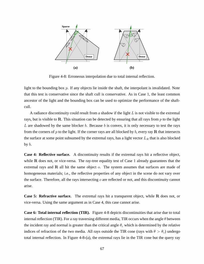
Sparse

(a) (b)

Dense Dense

Figure 4-8: Erroneous interpolation due to total internal reflection.

light to the bounding box p. If any objects lie inside the shaft, the interpolant is invalidated. Note

that this test is conservative since the shaft cull is conservative. As in Case 1, the least common

ancestor of the light and the bounding box can be used to optimize the performance of the shaft-

cull.

A radiance discontinuity could result from a shadow if the light L is not visible to the extremal

rays, but is visible toR. This situation can be detected by ensuring that all rays from p to the light

L are shadowed by the same blocker b. Because b is convex, it is only necessary to test the rays

from the corners of p to the light. If the corner rays are all blocked by b, every rayR that intersects

the surface at some point subsumed by the extremal rays, has a light vector LR that is also blocked

by b.

Case 4: Reflective surface. A discontinuity results if the extremal rays hit a reflective object,

while R does not, or vice-versa. The ray-tree equality test of Case 1 already guarantees that the

extremal rays and R all hit the same object o. The system assumes that surfaces are made of

homogeneous materials; i.e., the reflective properties of any object in the scene do not vary over

the surface. Therefore, all the rays intersecting o are reflected or not, and this discontinuity cannot

arise.

Case 5: Refractive surface. The extremal rays hit a transparent object, while R does not, or

vice-versa. Using the same argument as in Case 4, this case cannot arise.

Case 6: Total internal reflection (TIR). Figure 4-8 depicts discontinuities that arise due to total

internal reflection (TIR). For a ray traversing different media, TIR occurs when the angle θ between

the incident ray and normal is greater than the critical angle θc which is determined by the relative

indices of refraction of the two media. All rays outside the TIR cone (rays with θ > θc) undergo

total internal reflection. In Figure 4-8-(a), the extremal rays lie in the TIR cone but the query ray

67

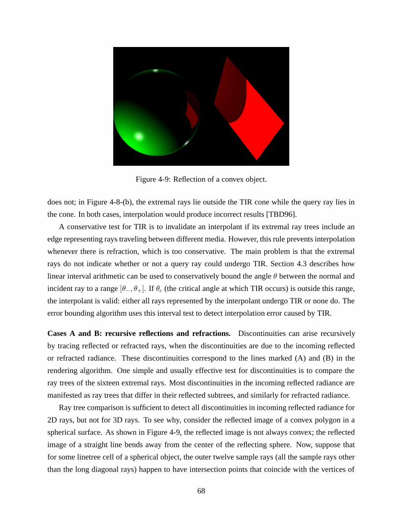
Figure 4-9: Reflection of a convex object.

does not; in Figure 4-8-(b), the extremal rays lie outside the TIR cone while the query ray lies in

the cone. In both cases, interpolation would produce incorrect results [TBD96].

A conservative test for TIR is to invalidate an interpolant if its extremal ray trees include an

edge representing rays traveling between different media. However, this rule prevents interpolation

whenever there is refraction, which is too conservative. The main problem is that the extremal

rays do not indicate whether or not a query ray could undergo TIR. Section 4.3 describes how

linear interval arithmetic can be used to conservatively bound the angle θ between the normal and

incident ray to a range [θ−, θ+]. If θc (the critical angle at which TIR occurs) is outside this range,

the interpolant is valid: either all rays represented by the interpolant undergo TIR or none do. The

error bounding algorithm uses this interval test to detect interpolation error caused by TIR.

Cases A and B: recursive reflections and refractions. Discontinuities can arise recursively

by tracing reflected or refracted rays, when the discontinuities are due to the incoming reflected

or refracted radiance. These discontinuities correspond to the lines marked (A) and (B) in the

rendering algorithm. One simple and usually effective test for discontinuities is to compare the

ray trees of the sixteen extremal rays. Most discontinuities in the incoming reflected radiance are

manifested as ray trees that differ in their reflected subtrees, and similarly for refracted radiance.

Ray tree comparison is sufficient to detect all discontinuities in incoming reflected radiance for

2D rays, but not for 3D rays. To see why, consider the reflected image of a convex polygon in a

spherical surface. As shown in Figure 4-9, the reflected image is not always convex; the reflected

image of a straight line bends away from the center of the reflecting sphere. Now, suppose that

for some linetree cell of a spherical object, the outer twelve sample rays (all the sample rays other

than the long diagonal rays) happen to have intersection points that coincide with the vertices of

68

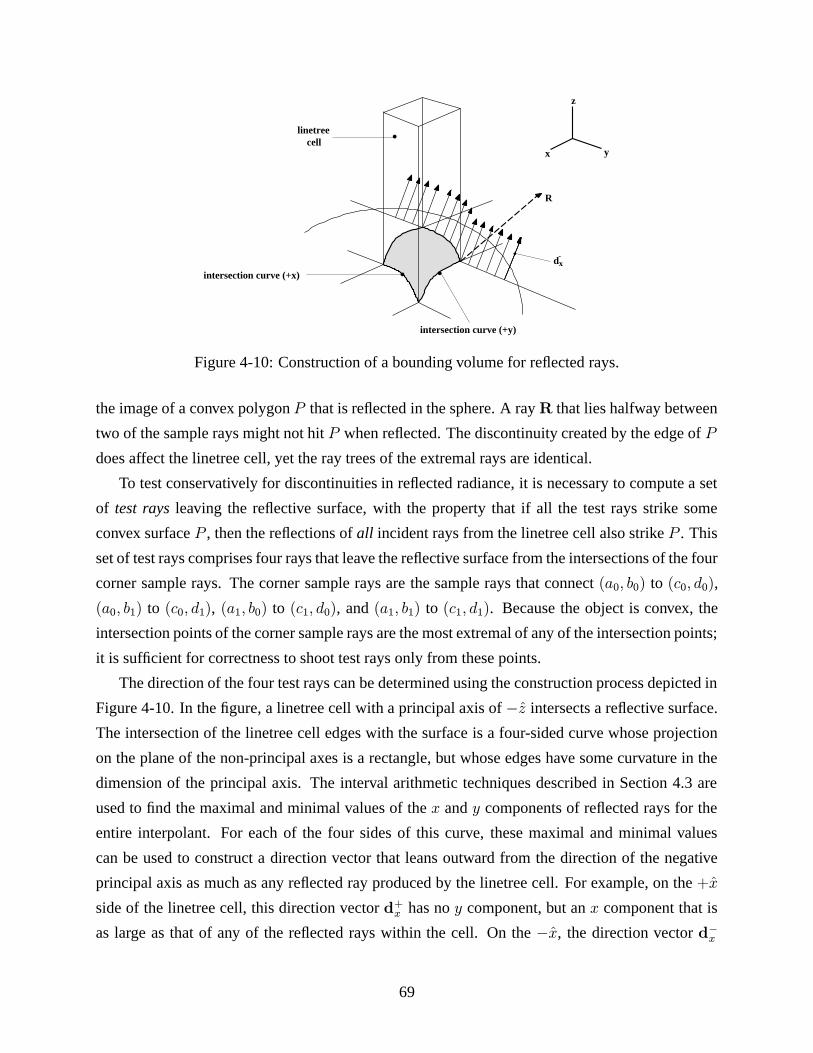
x y

z

intersection curve (+x)

dx-

R

linetreecell

intersection curve (+y)

Figure 4-10: Construction of a bounding volume for reflected rays.

the image of a convex polygon P that is reflected in the sphere. A rayR that lies halfway between

two of the sample rays might not hit P when reflected. The discontinuity created by the edge of P

does affect the linetree cell, yet the ray trees of the extremal rays are identical.

To test conservatively for discontinuities in reflected radiance, it is necessary to compute a set

of test raysleaving the reflective surface, with the property that if all the test rays strike some

convex surface P , then the reflections of all incident rays from the linetree cell also strike P . This

set of test rays comprises four rays that leave the reflective surface from the intersections of the four

corner sample rays. The corner sample rays are the sample rays that connect (a0, b0) to (c0, d0),

(a0, b1) to (c0, d1), (a1, b0) to (c1, d0), and (a1, b1) to (c1, d1). Because the object is convex, the

intersection points of the corner sample rays are the most extremal of any of the intersection points;

it is sufficient for correctness to shoot test rays only from these points.

The direction of the four test rays can be determined using the construction process depicted in

Figure 4-10. In the figure, a linetree cell with a principal axis of −z intersects a reflective surface.

The intersection of the linetree cell edges with the surface is a four-sided curve whose projection

on the plane of the non-principal axes is a rectangle, but whose edges have some curvature in the

dimension of the principal axis. The interval arithmetic techniques described in Section 4.3 are

used to find the maximal and minimal values of the x and y components of reflected rays for the

entire interpolant. For each of the four sides of this curve, these maximal and minimal values

can be used to construct a direction vector that leans outward from the direction of the negative

principal axis as much as any reflected ray produced by the linetree cell. For example, on the +x

side of the linetree cell, this direction vector d+x has no y component, but an x component that is

as large as that of any of the reflected rays within the cell. On the −x, the direction vector d−x

69

has no y component, but an x component that is at most as large as that of any reflected ray. The

x components that satisfy these conditions are the maximum and minimum computed by interval

analysis.

Now, imagine sliding the direction vector d−x associated with the −x side of the intersection

curve along that side, generating a surface consisting of all the points in space that are in the

given direction from some point along that side of the intersection curve. If the direction vector is

allowed to continue past the corners of the intersection curve at the same z value as the corner it

slides past, it generates an infinite surface. Repeating this process for all four sides of the curve,

a set of four surfaces is obtained. Together, these four surfaces bound all reflected rays from the

linetree cell.

Fortunately, the ray tracer does not need to construct an actual representation of these four

rather complex bounding surfaces. Each of the four surfaces intersects the two surfaces corre-

sponding to the adjacent sides of the intersection curve; the interface of any two of these surfaces

is a ray extending outward from a corner of the intersection curve. For each of the corners of the

intersection curve, there is such a ray; these rays are the four test rays. For example, consider

the intersection of the −x surface depicted in the figure with the +y surface. The direction of

the test ray that is the intersection of these surfaces is indicated by the dashed ray R in the fig-

ure. Its coordinates (x, y, z) can be computed from the coordinates for the d−x and d+y rays, which

have the form (x−, 0, z′) and (0, y+, z′′) respectively. The following equations uniquely define the

intersection ray R = (x, y, z) for this corner of the intersection curve:

x2 + y2 + z2 = 1x

x−=

z

z′y

y+=

z

z′′

The solution to these three equations is straightforward:

(zx−

z′)2 + (

zy+

z′′)2 + z2 = 1

x =zx−

z′

y =zy+

z′′

70

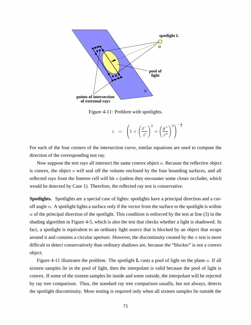
spotlight L

α

ο

pool oflight

points of intersectionof extremal rays

Figure 4-11: Problem with spotlights.

z =

1 +

(x−

z′

)2+

(y+

z′′

)2− 12

For each of the four corners of the intersection curve, similar equations are used to compute the

direction of the corresponding test ray.

Now suppose the test rays all intersect the same convex object o. Because the reflective object

is convex, the object o will seal off the volume enclosed by the four bounding surfaces, and all

reflected rays from the linetree cell will hit o (unless they encounter some closer occluder, which

would be detected by Case 1). Therefore, the reflected ray test is conservative.

Spotlights. Spotlights are a special case of lights: spotlights have a principal direction and a cut-

off angle α. A spotlight lights a surface only if the vector from the surface to the spotlight is within

α of the principal direction of the spotlight. This condition is enforced by the test at line (3) in the

shading algorithm in Figure 4-5, which is also the test that checks whether a light is shadowed. In

fact, a spotlight is equivalent to an ordinary light source that is blocked by an object that wraps

around it and contains a circular aperture. However, the discontinuity created by the α test is more

difficult to detect conservatively than ordinary shadows are, because the “blocker” is not a convex

object.

Figure 4-11 illustrates the problem. The spotlight L casts a pool of light on the plane o. If all

sixteen samples lie in the pool of light, then the interpolant is valid because the pool of light is

convex. If some of the sixteen samples lie inside and some outside, the interpolant will be rejected

by ray tree comparison. Thus, the standard ray tree comparison usually, but not always, detects

the spotlight discontinuity. More testing is required only when all sixteen samples lie outside the

71

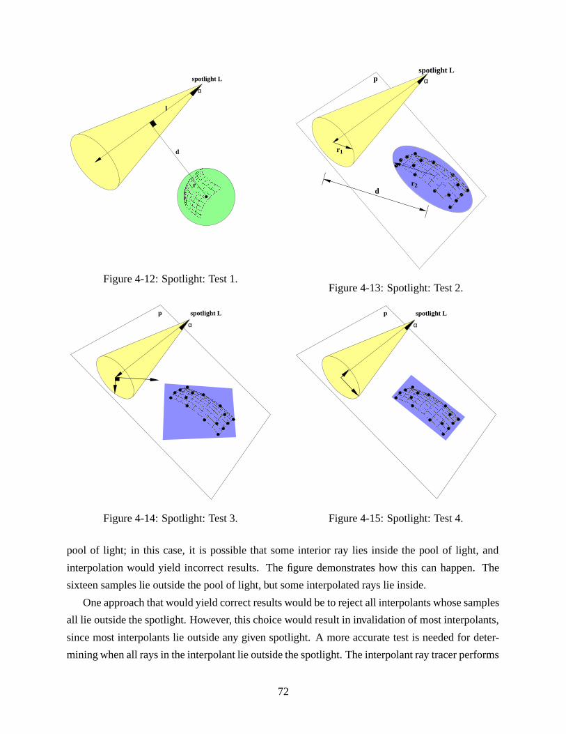
d

spotlight L

α

l

r

Figure 4-12: Spotlight: Test 1.

spotlight Lαp

d

r1

r2

Figure 4-13: Spotlight: Test 2.

spotlight L

α

p

Figure 4-14: Spotlight: Test 3.

spotlight L

α

p

Figure 4-15: Spotlight: Test 4.

pool of light; in this case, it is possible that some interior ray lies inside the pool of light, and

interpolation would yield incorrect results. The figure demonstrates how this can happen. The

sixteen samples lie outside the pool of light, but some interpolated rays lie inside.

One approach that would yield correct results would be to reject all interpolants whose samples

all lie outside the spotlight. However, this choice would result in invalidation of most interpolants,

since most interpolants lie outside any given spotlight. A more accurate test is needed for deter-

mining when all rays in the interpolant lie outside the spotlight. The interpolant ray tracer performs

72

a series of four tests to detect this condition. If any of the tests succeed, further testing is not nec-

essary because the interpolant is valid. If all the tests fail, the interpolant is considered invalid. The

ray tracer performs these tests in the order given below—from least expensive to most expensive,

and correspondingly, from most conservative to most accurate.

Test 1: The spotlight can be considered as an infinite cone in 3D. When an interpolant is built, a

sphere including all the points of intersection of the extremal rays is constructed, centered

on the center of mass of these points, as shown in Figure 4-12. A test that the cone and the

sphere do not intersect can be done quickly; the test is that d > r cosα + l tanα [Ama84].

If the sphere and cone do not intersect each other, the interpolant is valid. Otherwise, more

testing is required.

Test 2: Test 1 is conservative because the sphere enclosing the intersection points can be quite large.

A more precise test is used when Test 1 fails. The sixteen points of intersection are projected

onto a plane perpendicular to the principal direction of the spotlight, as shown in Figure 4-

13. The spotlight casts a perfectly circular region of light on this plane, with some radius

r1. A circle with some radius r2 is constructed that contains the sixteen projected points. If

d > (r1 + r2), there is no overlap between the spotlight’s pool of light and the interpolant,

and the interpolant is valid.

Test 3: Consider the case where the projected points lie along a thin long rectangle; the circle that

contains all the points can be too conservative. Therefore, if Test 2 fails, a two-dimensional

coordinate system is set up for the plane constructed in Test 2. The origin of this coordinate

system is at the point where the principal direction of the spotlight intersects the plane,

and the spotlight’s light is a circle with radius r1 around this origin. The projected points

are translated into this coordinate system and a bounding rectangle is constructed for the

translated points as shown in Figure 4-14. If the bounding rectangle does not intersect the

spotlight’s circle, the interpolant is valid.

Test 4: The size of the bounding rectangle in Test 3 depends on the axes of the new coordinate

system; therefore, Test 3 might fail because a suboptimal bounding rectangle is computed.

Test 4 addresses that problem by computing a new coordinate system with the same origin,

but different axes, to give a tight bounding rectangle around the projected points as shown

in Figure 4-15. This new coordinate system minimizes the average square distance of the

projected points from one of the new axes; its basis vectors are computed by diagonalizing

the 2× 2 inertia tensor for the projected points [LL76]. While Test 4 is more expensive than

73

Test 3, it produces a tighter bounding rectangle for the points, as can be seen in Figure 4-15.

The same intersection test as in Test 3 is performed again with the new bounding rectangle.

The most accurate test would be to compute the convex hull of the projected points in the

plane and test whether the convex hull intersects the circle. This test would be more expen-

sive and complex than Test 4, and seems unlikely to improve accuracy substantially.

4.3 Non-linear radiance variations

The previous section has shown how the various sources of discontinuities in an interpolant can be

detected conservatively. Once discontinuities are detected, the only remaining source of interpola-

tion error is the computation of the local diffuse and shading component itself (indicated as NL in

the shading algorithm shown in Figure 4-5). Quadrilinear interpolation approximates radiance well

in most regions of line space that are free of discontinuities, but it is not accurate where radiance

varies in a significantly non-linear fashion; for example, at specular highlights and diffuse peaks.

This section shows how a generalized interval arithmetic can be used to conservatively and

tightly bound the deviation between interpolated radiance and base radiance for all rays represented

by a linetree cell (where base radiance is the radiance computed by the base ray tracer).

4.3.1 Motivation

Radiance can vary non-linearly across a surface; this effect is particularly noticeable at radiance

peaks such as specular highlights and diffuse highlights. If interpolation is performed without

testing for these non-linear radiance variations, images will have visual artifacts like those shown

in Figure 4-16. On the top row of the figure, images depict a specular highlight for a shiny sphere

and a diffuse highlight for a plane. The bottom row of the figure shows images in which the ray

tracer does not correctly identify the non-linear radiance variations, and the specular and diffuse

highlights are rendered incorrectly.

The reason that interpolation error can arise is depicted in Figure 4-17 for the case of diffuse

radiance in two dimensions. Similar scenarios can be constructed for specular radiance. In the

figure, the incoming eye rayR strikes the surface at the diffuse radiance peak, because the normal

at that point on the surface points directly at the light source, and diffuse radiance is proportional to

N · L. Now, consider the four intersection points of the sample rays of the linetree cell containing

the incoming eye ray. None of the surface normals at these intersection points are directed at

the light. Therefore, bilinear interpolation across this linetree cell will result in the eye ray being

74

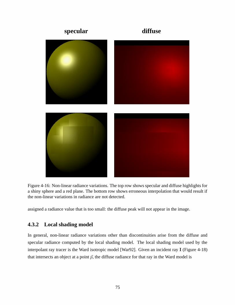
diffusespecular

Figure 4-16: Non-linear radiance variations. The top row shows specular and diffuse highlights fora shiny sphere and a red plane. The bottom row shows erroneous interpolation that would result ifthe non-linear variations in radiance are not detected.

assigned a radiance value that is too small: the diffuse peak will not appear in the image.

4.3.2 Local shading model

In general, non-linear radiance variations other than discontinuities arise from the diffuse and

specular radiance computed by the local shading model. The local shading model used by the

interpolant ray tracer is the Ward isotropic model [War92]. Given an incident ray I (Figure 4-18)

that intersects an object at a point $p, the diffuse radiance for that ray in the Ward model is

75

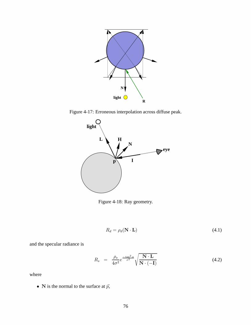
lightR

N

Figure 4-17: Erroneous interpolation across diffuse peak.

NL

I

H

p

eye

light

Figure 4-18: Ray geometry.

Rd = ρd(N · L) (4.1)

and the specular radiance is

Rs =ρs

4σ2e− tan2 ασ2

√N · LN · (−I) (4.2)

where

• N is the normal to the surface at $p,

76

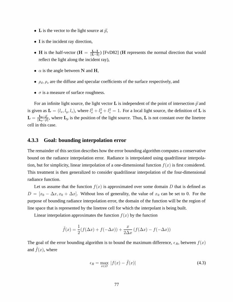
• L is the vector to the light source at $p,

• I is the incident ray direction,

• H is the half-vector (H = L−I‖L−I‖ ) [FvD82] (H represents the normal direction that would

reflect the light along the incident ray),

• α is the angle betweenN andH,

• ρd, ρs are the diffuse and specular coefficients of the surface respectively, and

• σ is a measure of surface roughness.

For an infinite light source, the light vector L is independent of the point of intersection $p and

is given as L = (lx, ly, lz), where l2x + l2y + l2z = 1. For a local light source, the definition of L is

L = Lp−�p‖Lp−�p‖ , where Lp is the position of the light source. Thus, L is not constant over the linetree

cell in this case.

4.3.3 Goal: bounding interpolation error

The remainder of this section describes how the error bounding algorithm computes a conservative

bound on the radiance interpolation error. Radiance is interpolated using quadrilinear interpola-

tion, but for simplicity, linear interpolation of a one-dimensional function f(x) is first considered.

This treatment is then generalized to consider quadrilinear interpolation of the four-dimensional

radiance function.

Let us assume that the function f(x) is approximated over some domain D that is defined as

D = [x0 − ∆x, x0 + ∆x]. Without loss of generality, the value of x0 can be set to 0. For the

purpose of bounding radiance interpolation error, the domain of the function will be the region of

line space that is represented by the linetree cell for which the interpolant is being built.

Linear interpolation approximates the function f(x) by the function

f(x) =1

2(f(∆x) + f(−∆x)) +

x

2∆x(f(∆x)− f(−∆x))

The goal of the error bounding algorithm is to bound the maximum difference, εR, between f(x)

and f(x), where

εR = maxx∈D

|f(x)− f(x)| (4.3)

77

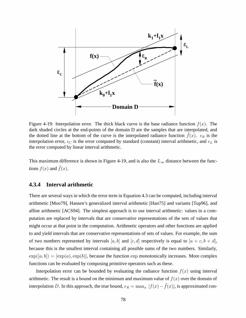
f(x)

k1+l1x

k0+l1x

f(x)~

εR

εL

Domain D

εC

Figure 4-19: Interpolation error. The thick black curve is the base radiance function f(x). Thedark shaded circles at the end-points of the domain D are the samples that are interpolated, andthe dotted line at the bottom of the curve is the interpolated radiance function f(x). εR is theinterpolation error, εC is the error computed by standard (constant) interval arithmetic, and εL isthe error computed by linear interval arithmetic.

This maximum difference is shown in Figure 4-19, and is also the L∞ distance between the func-

tions f(x) and f(x).

4.3.4 Interval arithmetic

There are several ways in which the error term in Equation 4.3 can be computed, including interval

arithmetic [Moo79], Hansen’s generalized interval arithmetic [Han75] and variants [Tup96], and

affine arithmetic [ACS94]. The simplest approach is to use interval arithmetic: values in a com-

putation are replaced by intervals that are conservative representations of the sets of values that

might occur at that point in the computation. Arithmetic operators and other functions are applied

to and yield intervals that are conservative representations of sets of values. For example, the sum

of two numbers represented by intervals [a, b] and [c, d] respectively is equal to [a + c, b + d],

because this is the smallest interval containing all possible sums of the two numbers. Similarly,

exp([a, b]) = [exp(a), exp(b)], because the function exp monotonically increases. More complex

functions can be evaluated by composing primitive operators such as these.

Interpolation error can be bounded by evaluating the radiance function f(x) using interval

arithmetic. The result is a bound on the minimum and maximum value of f(x) over the domain of

interpolation D. In this approach, the true bound, εR = maxx |f(x)− f(x)|, is approximated con-

78

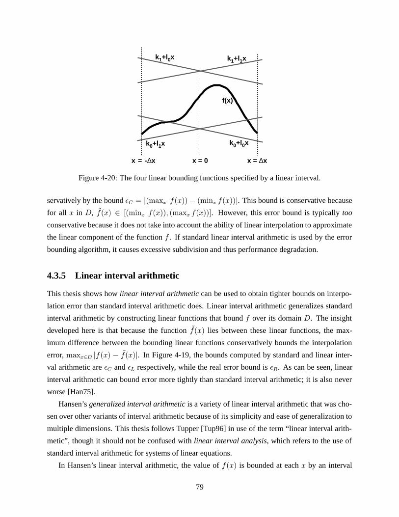
x = 0 x = ∆xx = -∆x

f(x)

k1+l1x

k0+l0x

k1+l0x

k0+l1x

Figure 4-20: The four linear bounding functions specified by a linear interval.

servatively by the bound εC = |(maxx f(x))− (minx f(x))|. This bound is conservative because

for all x in D, f(x) ∈ [(minx f(x)), (maxx f(x))]. However, this error bound is typically too

conservative because it does not take into account the ability of linear interpolation to approximate

the linear component of the function f . If standard linear interval arithmetic is used by the error

bounding algorithm, it causes excessive subdivision and thus performance degradation.

4.3.5 Linear interval arithmetic

This thesis shows how linear interval arithmeticcan be used to obtain tighter bounds on interpo-

lation error than standard interval arithmetic does. Linear interval arithmetic generalizes standard

interval arithmetic by constructing linear functions that bound f over its domain D. The insight

developed here is that because the function f(x) lies between these linear functions, the max-

imum difference between the bounding linear functions conservatively bounds the interpolation

error, maxx∈D |f(x) − f(x)|. In Figure 4-19, the bounds computed by standard and linear inter-

val arithmetic are εC and εL respectively, while the real error bound is εR. As can be seen, linear

interval arithmetic can bound error more tightly than standard interval arithmetic; it is also never

worse [Han75].

Hansen’s generalized interval arithmeticis a variety of linear interval arithmetic that was cho-

sen over other variants of interval arithmetic because of its simplicity and ease of generalization to

multiple dimensions. This thesis follows Tupper [Tup96] in use of the term “linear interval arith-

metic”, though it should not be confused with linear interval analysis, which refers to the use of

standard interval arithmetic for systems of linear equations.

In Hansen’s linear interval arithmetic, the value of f(x) is bounded at each x by an interval

79

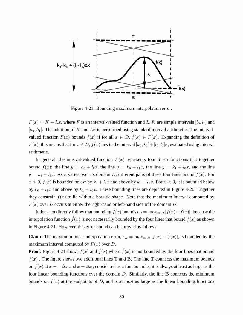
f(x)

f(x)~

T

B

k1-k 0 + (l1- l 0)∆x

εR

Figure 4-21: Bounding maximum interpolation error.

F (x) = K + Lx, where F is an interval-valued function and L,K are simple intervals [l0, l1] and

[k0, k1]. The addition of K and Lx is performed using standard interval arithmetic. The interval-

valued function F (x) bounds f(x) if for all x ∈ D, f(x) ∈ F (x). Expanding the definition of

F (x), this means that for x ∈ D, f(x) lies in the interval [k0, k1]+[l0, l1]x, evaluated using interval

arithmetic.

In general, the interval-valued function F (x) represents four linear functions that together

bound f(x): the line y = k0 + l0x, the line y = k0 + l1x, the line y = k1 + l0x, and the line

y = k1 + l1x. As x varies over its domain D, different pairs of these four lines bound f(x). For

x > 0, f(x) is bounded below by k0 + l0x and above by k1 + l1x. For x < 0, it is bounded below

by k0 + l1x and above by k1 + l0x. These bounding lines are depicted in Figure 4-20. Together

they constrain f(x) to lie within a bow-tie shape. Note that the maximum interval computed by

F (x) over D occurs at either the right-hand or left-hand side of the domain D.

It does not directly follow that bounding f(x) bounds εR = maxx∈D |f(x)− f(x)|, because the

interpolation function f(x) is not necessarily bounded by the four lines that bound f(x) as shown

in Figure 4-21. However, this error bound can be proved as follows.

Claim: The maximum linear interpolation error, εR = maxx∈D |f(x) − f(x)|, is bounded by the

maximum interval computed by F (x) over D.

Proof: Figure 4-21 shows f(x) and f(x) where f(x) is not bounded by the four lines that bound

f(x) . The figure shows two additional lines T and B. The line T connects the maximum bounds

on f(x) at x = −∆x and x = ∆x; considered as a function of x, it is always at least as large as the

four linear bounding functions over the domain D. Similarly, the line B connects the minimum

bounds on f(x) at the endpoints of D, and is at most as large as the linear bounding functions

80

over D. Because T and B bound the linear bounding functions, T and B also bound f(x). Also,

T and B bound the linear interpolation function f(x). Therefore, the distance between f(x) and

f(x) is at most as large as the distance between T and B, which is k1 − k0 + ∆x(l1 − l0) for

all x. Therefore, the maximum linear interpolation error is bounded by this distance, which is the

maximum interval computed by F (x) over D.

This proves that the maximum interpolation error εR is bounded by the maximum interval

computed by F (x) over D, which occurs at either the right-hand or left-hand side of the domain

D.

This approach generalizes to functions of several variables xi. Given a function f(x1, . . . , xn)

where each of the variables xi varies over [−∆xi,∆xi], a multi-variate linear interval-valued func-

tion can be constructed that bounds it. This function takes the form

F (x) = K +∑i

Lixi

where K and all of the Li are intervals. For compactness, the set of n + 1 intervals specifying a

linear interval-valued function are called a linear interval for the function f that they bound. For

all points x = (x1, . . . , xn) such that xi ∈ [−∆xi,∆xi], the value of the function f is bounded by

the interval produced by F : f(x) ∈ F (x).

The goal of the ray tracer is to bound radiance, a function of four variables: f(a, b, c, d). A

linear interval F that bounds radiance can be specified as a constant interval K and four intervals

La, Lb, Lc, Ld. Just as in the single-variable case, the maximum error introduced by quadrilinear

interpolation is at most as large as the size of the largest interval produced by F over its domain.

This largest interval occurs at one of the sixteen corner points of the domain, so it can be computed

as the size of the largest interval computed by evaluating F at the sixteen corner points of D.

Arithmetic operators on linear intervals. A linear interval that bounds the radiance function

can be produced using the standard approach for interval arithmetic: the shading computation

performed by the ray tracer is broken down into a series of simple operations, and these operations

are performed on linear intervals rather than on ordinary scalars. This approach requires rules for

propagating linear intervals through each of the operations being performed.

For example, consider the multiplication of two quantities for which linear intervals are known:

the product of two functions f(x) and g(x). Suppose that these two functions are bounded by linear

intervals Kf +∑

Lfixi and Kg+∑

Lgixi, respectively. The product h(x) = f(x)g(x) is bounded

81

by a linear interval with components Kh and Lhi that are computed as follows [Han75]:

Kh = Kf ·Kg +∑i

[0,∆x2i ]LfiLgi

Lhi = Kf · Lgi +Kg · Lfi + Lfi∑j �=i

[−∆xj ,∆xj ] · Lgj

Similar rules are derived for the other operations needed to compute shading: 1f(x)

,√f(x), and

ef(x). For example, the reciprocal of a linear interval h(x) = 1f(x)

is computed as follows:

Kh = 1/Kf

Lhi =−Lfi

Kf · (Kf +∑j[−∆xj ,∆xj ]Lfj)

General functions on linear intervals. Hansen’s approach to more general functions such as

ex is to use the first-order Taylor expansion of the function to generate a rule for propagating

linear intervals. The error bounding algorithm presented here improves on this approach by using

second-order Taylor expansions that result in tighter error bounds.

According to Taylor’s theorem [DB69], when n terms of the Taylor series are used to approxi-

mate f(x) over the domain D = [−∆x,∆x], the remainder Rn is the error that results from using

this truncated approximation:

∀x∈D∃ξ∈D f(x) = f(x0) + f ′(x0)(x− x0) + . . .+ f (n−1)(x0)(x− x0)

n−1

(n− 1)!+ f (n)(ξ)

(x− x0)n

n!

Rn(x) = f (n)(ξ)(x− x0)

n

n!

For each x in the domain D, ξ is some other point in the domain D; ξ is a function of the x chosen.

The same theorem generalizes to functions of several variables.

Consider the expression f(y(x)) where y(x) is a function of x and f is a scalar function. This

expression is a function of x. Assume that the function y(x) is bounded by the linear interval

K +∑

Lixi. A rule is needed for producing a linear interval for f(y(x)). In Hansen’s approach,

this linear interval is computed conservatively by expanding f(y(x)) around x = 0 to terms linear

in xi (n = 1 in Taylor’s theorem). For the moment, this result is presented without justification:

f(y(x)) ∈ f(K) + f ′(Y )∑

Lixi

The expression on the right-hand side is evaluated using standard interval arithmetic. In this equa-

tion, the interval variable Y is a standard interval capturing the maximum range of the variable y:

82

that is, Y = K +∑

Li[−∆xi,∆xi]. This formula leads directly to the rule for the resulting linear

interval Kf , Lfi:

Kf = f(K)

Lfi = f ′(Y )Li

For example, with this rule the expression exp(K + Lx) produces a new linear interval eK +

eY Lx. Of course, exponentiation is particularly convenient for this rule because f = f ′.

Hansen does not prove this general rule to be sound, though it can be done as follows.

Claim: The function f(y(x)) is bounded by the linear interval

f(K) + f ′(Y )∑

Lixi

if y(x) is bounded by the linear interval K +∑

Lixi, and Y = K +∑

Li[−∆xi,∆xi].

Proof: Consider the evaluation of the function f(y(x)) at some particular point x∗. Because y(x)

is bounded by the linear interval K +∑

Lixi, there is some scalar k ∈ K and li ∈ Li (for each

i) such that y(x∗) = k +∑i lix

∗i . Now, define a new function y∗ that is equal to y at the point

x∗: y∗(x) = k +∑i lixi. To evaluate f(y(x)) at the point x = x∗, the function f(y∗(x)) can be

evaluated at x = x∗ instead. This function f(y∗(x)) can be expanded in a first-order Taylor series:

f(y∗(x)) = f(y∗(0)) +∑i

xi∂f(y∗(x))

∂xi

∣∣∣∣∣x=ξ(x)

= f(k) +∑i

xif′(y∗(ξ(x)))

∂y∗(x)∂xi

∣∣∣∣∣x=ξ(x)

(using the chain rule)

= f(k) +∑i

xif′(y∗(ξ(x)))li

Now, observe that k ∈ K, y∗(ξ(x)) ∈ Y , and li ∈ Li. Therefore, f(y∗(x)) ∈ f(K) +

f ′(Y )∑

Lixi. The interval Y effectively allows the variable ξ in Taylor’s theorem to take on any

value in D; this is a conservative position to take, since it assumes nothing about ξ. At the point

x∗, it is also the case that f(y(x∗)) ∈ K + f ′(Y )∑

Lix∗i . Since this is the case for any x∗ ∈ D, it

is proved that the expression f(y(x)) is bounded by the linear interval K + f ′(Y )∑

Lixi.

Hansen’s approach yields conservative intervals, but the resulting error estimates are often

overly conservative because the rule expands the intervals Lfi. The approach presented above can

83

be extended to a second-order Taylor expansion that usually results in tighter intervals. Using

reasoning similar to that for the first-order expansion, the following relation is derived:

f(y(x)) ∈ f(K) + f ′(K)∑

Lixi +∑i

∑j

1

2f ′′(Y )LiLjxixj

Note that the new terms linear in xi are tighter than in the first-order formulation because f ′

is applied to K rather than to the wider interval Y . However, this result does not directly lead to

a rule for computing the linear interval for f(y), because the second-order terms f ′′(Y )LiLjxixj

must be dealt with. To arrive at a linear interval, these terms must be folded into either the constant

or linear terms of the linear interval. For tight bounds, it is important to fold the diagonal second-

order terms (i = j) into the constant term of the resulting linear interval. This approach allows the

use of the tighter interval arithmetic rule for squaring a number [Moo79]. (The rule is applied to

the term (Lixi)2.) The other, non-diagonal second-order terms (i = j) can be folded into either

the constant term or the linear terms. Empirically, it seems not to make much difference which

approach is taken.

The non-diagonal terms are folded into the constant term as follows:

f(y(x)) ∈ f(K) + f ′(K)∑i

Lixi

+1

2f ′′(Y )

∑i

L2i [0,∆x2i ]

+ f ′′(Y )∑i

∑j<i

LiLj [−∆xi,∆xi][−∆xj ,∆xj ]

Using the definition li = max(|Li|), the rule for applying f to the linear interval y can be

expressed in a computationally efficient form that is used by the error bounding algorithm:

Kf = f(K) +

[0,

1

2

∑i

l2i∆x2i

]f ′′(Y ) + [−1, 1]f ′′(Y )

∑i

∑j<i

lilj∆xi∆xj

Lfi = f ′(K)Li

Alternatively, the non-diagonal terms can be folded into the linear terms of the result by factor-

ing out xi and shifting the mixed term into the corresponding linear term for xi:

f(y(x)) ∈ f(K) + f ′(K)∑

Lixi +

[0,

1

2

∑i

∆l2i x2i

]f ′′(Y )

84

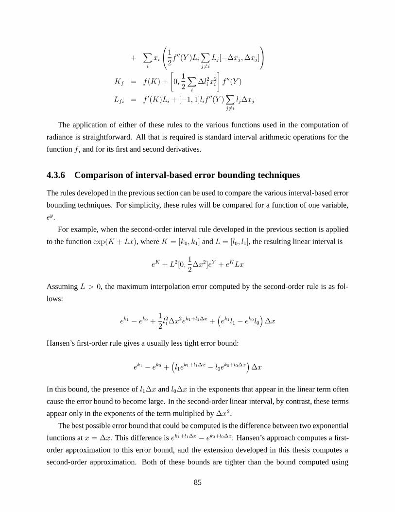
+∑i

xi

1

2f ′′(Y )Li

∑j �=i

Lj [−∆xj ,∆xj ]

Kf = f(K) +

[0,

1

2

∑i

∆l2i x2i

]f ′′(Y )

Lfi = f ′(K)Li + [−1, 1]lif ′′(Y )∑j �=i

lj∆xj

The application of either of these rules to the various functions used in the computation of

radiance is straightforward. All that is required is standard interval arithmetic operations for the

function f , and for its first and second derivatives.

4.3.6 Comparison of interval-based error bounding techniques

The rules developed in the previous section can be used to compare the various interval-based error

bounding techniques. For simplicity, these rules will be compared for a function of one variable,

ey.

For example, when the second-order interval rule developed in the previous section is applied

to the function exp(K + Lx), where K = [k0, k1] and L = [l0, l1], the resulting linear interval is

eK + L2[0,1

2∆x2]eY + eKLx

Assuming L > 0, the maximum interpolation error computed by the second-order rule is as fol-

lows:

ek1 − ek0 +1

2l21∆x2ek1+l1∆x +

(ek1l1 − ek0l0

)∆x

Hansen’s first-order rule gives a usually less tight error bound:

ek1 − ek0 +(l1ek1+l1∆x − l0e

k0+l0∆x)∆x

In this bound, the presence of l1∆x and l0∆x in the exponents that appear in the linear term often

cause the error bound to become large. In the second-order linear interval, by contrast, these terms

appear only in the exponents of the term multiplied by ∆x2.

The best possible error bound that could be computed is the difference between two exponential

functions at x = ∆x. This difference is ek1+l1∆x − ek0+l0∆x. Hansen’s approach computes a first-

order approximation to this error bound, and the extension developed in this thesis computes a

second-order approximation. Both of these bounds are tighter than the bound computed using

85

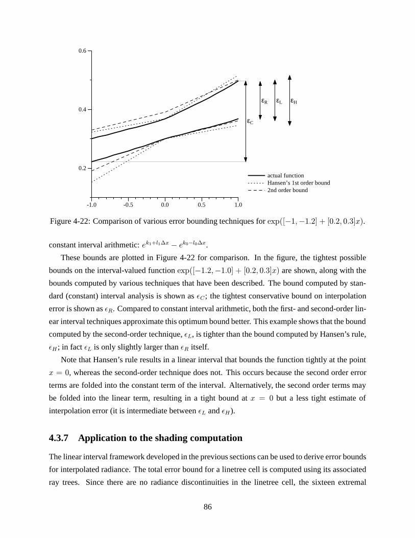
-1.0 -0.5 0.0 0.5 1.0

0.2

0.4

0.6

actual functionHansen’s 1st order bound2nd order bound

εC

εR εL εH

Figure 4-22: Comparison of various error bounding techniques for exp([−1,−1.2] + [0.2, 0.3]x).

constant interval arithmetic: ek1+l1∆x − ek0−l0∆x.

These bounds are plotted in Figure 4-22 for comparison. In the figure, the tightest possible

bounds on the interval-valued function exp([−1.2,−1.0] + [0.2, 0.3]x) are shown, along with the

bounds computed by various techniques that have been described. The bound computed by stan-

dard (constant) interval analysis is shown as εC ; the tightest conservative bound on interpolation

error is shown as εR. Compared to constant interval arithmetic, both the first- and second-order lin-

ear interval techniques approximate this optimum bound better. This example shows that the bound

computed by the second-order technique, εL, is tighter than the bound computed by Hansen’s rule,

εH ; in fact εL is only slightly larger than εR itself.

Note that Hansen’s rule results in a linear interval that bounds the function tightly at the point

x = 0, whereas the second-order technique does not. This occurs because the second order error

terms are folded into the constant term of the interval. Alternatively, the second order terms may

be folded into the linear term, resulting in a tight bound at x = 0 but a less tight estimate of

interpolation error (it is intermediate between εL and εH ).

4.3.7 Application to the shading computation

The linear interval framework developed in the previous sections can be used to derive error bounds

for interpolated radiance. The total error bound for a linetree cell is computed using its associated

ray trees. Since there are no radiance discontinuities in the linetree cell, the sixteen extremal

86

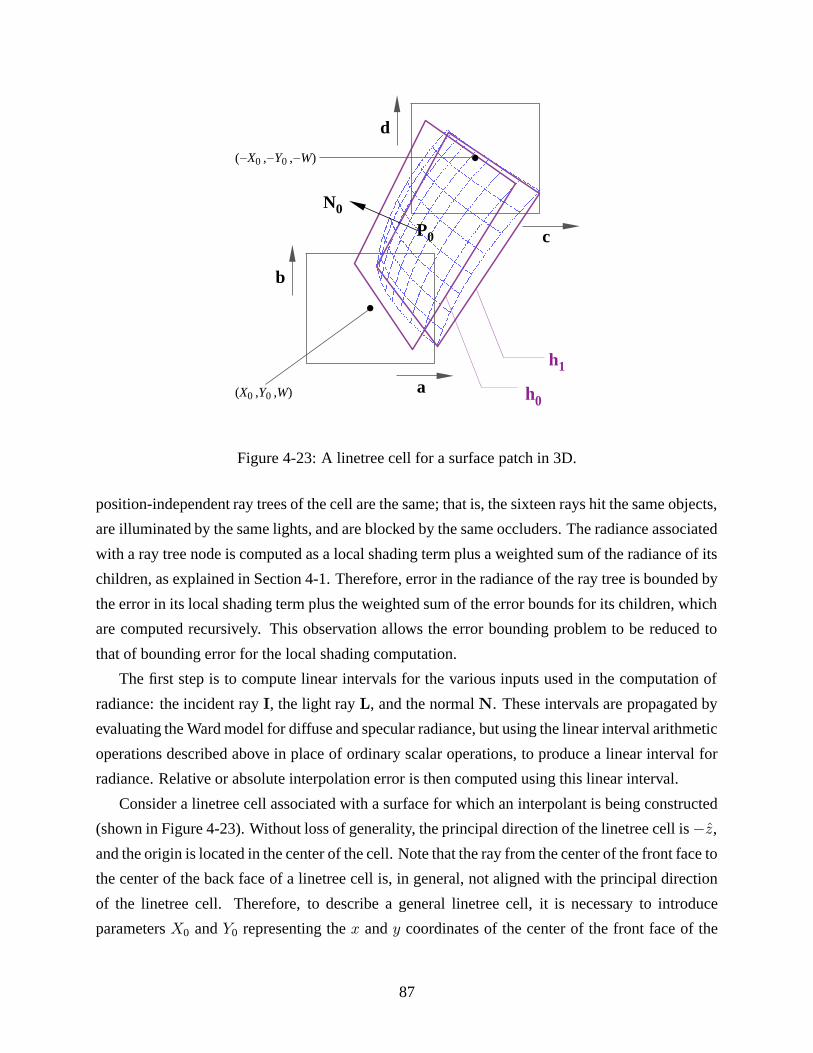
N0

(−X0 ,−Y0 ,−W)

P0

a

b

h0

h1

d

c

(X0 ,Y0 ,W)

Figure 4-23: A linetree cell for a surface patch in 3D.

position-independent ray trees of the cell are the same; that is, the sixteen rays hit the same objects,

are illuminated by the same lights, and are blocked by the same occluders. The radiance associated

with a ray tree node is computed as a local shading term plus a weighted sum of the radiance of its

children, as explained in Section 4-1. Therefore, error in the radiance of the ray tree is bounded by

the error in its local shading term plus the weighted sum of the error bounds for its children, which

are computed recursively. This observation allows the error bounding problem to be reduced to

that of bounding error for the local shading computation.

The first step is to compute linear intervals for the various inputs used in the computation of

radiance: the incident ray I, the light ray L, and the normalN. These intervals are propagated by

evaluating the Ward model for diffuse and specular radiance, but using the linear interval arithmetic

operations described above in place of ordinary scalar operations, to produce a linear interval for

radiance. Relative or absolute interpolation error is then computed using this linear interval.

Consider a linetree cell associated with a surface for which an interpolant is being constructed

(shown in Figure 4-23). Without loss of generality, the principal direction of the linetree cell is−z,

and the origin is located in the center of the cell. Note that the ray from the center of the front face to

the center of the back face of a linetree cell is, in general, not aligned with the principal direction

of the linetree cell. Therefore, to describe a general linetree cell, it is necessary to introduce

parameters X0 and Y0 representing the x and y coordinates of the center of the front face of the

87

linetree cell. The linetree cell is assumed to extend along the principal direction from −W to W .

Because the origin is at the center of the cell the cell’s front face is centered on (X0, Y0,W ) and its

back face is centered on (−X0,−Y0,−W ).

Incident ray I. Since the front and back faces of the linetree cell are at z = W and z = −Wrespectively, a ray parameterized by (a, b, c, d) represents a ray in 3D space from (a+X0, b+Y0,W )

to (c−X0, d− Y0,−W ). Therefore, the unnormalized incident ray is:

I = (c− a− 2X0, d− b− 2Y0,−2W )

Since each component of I is a simple linear function of the variables (a, b, c, d), the cor-

responding linear intervals are computed trivially. For example, the x-component of I is Ix =

−2X0+(−1)a+(−1)c, and the linear interval representation for Ix is [−2X0,−2X0]+[−1,−1]a+[1, 1]c. The incident ray is normalized by computing the linear interval for 1√

I2x+I2y+I

2z

, where each

of the operations used—division, square, square root, and addition—are the linear interval opera-

tions defined in the previous section.

Light ray L. For an infinite light source, the light vector is L = (lx, ly, lz), where l2x+ l2y+ l2z = 1.

The linear interval representation for the x-component of L is trivial: [lx, lx]. For a local light

source, L = Lp−�p‖Lp−�p‖ , where Lp is the position of the light source. The linear interval representation

for L is computed from the linear interval for $p using the interval operations described in the

previous section. The linear interval representation for the point of intersection $p is computed as

below.

Point of intersection $p. The point of intersection $p of the incident ray I with the surface lies on

I, and can be parameterized by its distance t from the front face:

$p = (X0 + a, Y0 + b,W ) + t I (4.4)

A conservative linear interval for the components of $p can be constructed in several ways with

varying degrees of precision. First, a simple way of conservatively bounding the intersection point

for any convex surface is described. Consider the ray R0 from the middle of the linetree’s front

face to the middle of its back face. R0 intersects the surface at the pointP0, and the normal at that

point is N0. Figures 4-24 and 4-23 depict this construction in 2D and 3D respectively. The plane

88

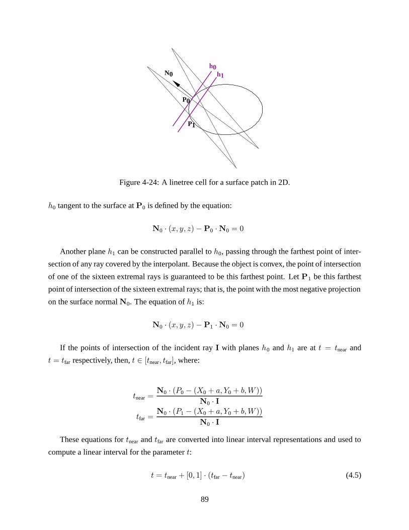
N0h0

h1

P1

P0

Figure 4-24: A linetree cell for a surface patch in 2D.

h0 tangent to the surface at P0 is defined by the equation:

N0 · (x, y, z)−P0 ·N0 = 0

Another plane h1 can be constructed parallel to h0, passing through the farthest point of inter-

section of any ray covered by the interpolant. Because the object is convex, the point of intersection

of one of the sixteen extremal rays is guaranteed to be this farthest point. Let P1 be this farthest

point of intersection of the sixteen extremal rays; that is, the point with the most negative projection

on the surface normalN0. The equation of h1 is:

N0 · (x, y, z)−P1 ·N0 = 0

If the points of intersection of the incident ray I with planes h0 and h1 are at t = tnear and

t = tfar respectively, then, t ∈ [tnear, tfar], where:

tnear =N0 · (P0 − (X0 + a, Y0 + b,W ))

N0 · Itfar =

N0 · (P1 − (X0 + a, Y0 + b,W ))

N0 · IThese equations for tnear and tfar are converted into linear interval representations and used to

compute a linear interval for the parameter t:

t = tnear + [0, 1] · (tfar − tnear) (4.5)

89

The linear interval for $p is then computed by substituting Equation 4.5 into Equation 4.4.

There is another option for computing linear intervals for $p when the point of intersection can

be computed analytically. For example, consider a general quadric surface in three dimensions,

defined by the following implicit equation:

Ax2 +By2 + Cz2 +Dxy + Eyz + Fxz +Gx+Hy + Iz + J = 0 (4.6)

Substituting $p = (x, y, z) = (X0 + a, Y0 + b,W ) + t I, gives a quadratic in t, which can be

solved to give a linear interval for $p.

NormalN. The vectorN normal to the surface at the intersection point is used in the computation

of diffuse and specular radiance: it appears in the termsN·I,N·L, andN·H. The surface normal at

the intersection point varies across the linetree cell; it is a function of (a, b, c, d). There are various

options for constructing the linear intervals that conservatively approximateN. If little information

about the surface within the linetree cell is available, the normal can be bounded using a constant

interval bound. While this characterization is not precise, it will bound error conservatively.

For quadric surfaces and other surfaces that can be characterized analytically, tighter bounds

can be obtained for the normal by normalizing the gradient of the implicit equation defining the

surface. For the quadric surface described by Equation 4.6, the unnormalized normal vector is

(2Ax+Dy + Fz +G, 2By +Dx+ Ez +H, 2Cz + Ey + Fx+ I)

As described earlier, the point of intersection $p = (x, y, z) can be expressed as a linear inter-

val. This solution is substituted into the normal vector formula, allowing the normal vector to be

bounded by linear intervals.

This approach can be extended to support spline patches. The surface intersection point can be

bounded by the two-plane technique described above. Normals can be bounded to varying degrees

of precision. A simple approach is to use constant intervals to bound the normals; a more accurate

approach is to compute linear intervals for the surface parameters (u, v) using interval-based root

finding [Han75]. The normal can then be computed using these parameters.

Other issues. One important technique to improve the precision of interval analysis for radiance is

to treat the term exp( 1σ2

tan2 α), which appears in the formula for specular radiance, as a primitive

linear interval operator. Although exp and tan are both functions that tend to amplify error, this

term computes a Gaussian function over tanα, and Gaussians are well-behaved regardless of the

domain of evaluation. A primitive linear interval operator can exploit this property of a Gaussian

90

function.

Because α is the angle between the vectorsN and H, this term can be evaluated more simply

by using the following equality:

tan2α = 1− 1

(N ·H)2

For this reason, a new linear interval operator is added that computes the function exp( 1σ2(1− 1

x2)),

which is applied in the computation of radiance with x = N ·H. The linear interval rule for this

function is obtained using the second-order Taylor expansion technique described in Section 4.3.3.

This approach yields a much tighter error bound than simple composition of the linear interval

rules for exponentiation and division does. Without this optimization, the error bound often di-

verges even for small linetree cells, preventing interpolation. Thus, this optimization is crucial for

good performance.

4.3.8 Error refinement

Figures 4-25 and 4-26 demonstrate the error refinement process for a specular sphere and a diffuse

plane. The top row of each figure shows the sphere and plane rendered without testing for non-

linearity; visible artifacts can be seen around the specular and diffuse highlights. The bottom row

shows the sphere and plane rendered with non-linearity detection enabled and ε = 0.2 and 0.1 re-

spectively. The system automatically detects the need for refinement around highlights and refines

interpolants that exceed the user-specified error bound. The image quality improves (bottom row)

and the linetrees are increasingly subdivided, as shown in the linetree visualization on the right.

Figure 4-27 shows a more complex scene containing many primitives (described in Section 7).

Non-linearity detection substantially reduces error and eliminates visual artifacts (shown in the

bottom row). The difference images in the right column show the error in interpolated radiance for

the images on the left. Because this error is subtle, the difference images have been scaled by a

factor of 4 for the purpose of visualization.

An interesting observation is that the error intervals can be used to subdivide linetree cells

more effectively. The error bound computed for an interpolant specifies intervals for each of the

four axes; the axes with larger intervals (that is, more error) are subdivided preferentially. This

error-driven subdivisionis discussed further in the next section.

Figure 4-28 shows the actual and interpolated radiance for one scan-line of the image in Fig-

ure 4-26; Figure 4-29 depicts actual and bounded error for that scan-line. The scan-line passes

through the diffuse peak of that image. The x-axis represents the pixels of the scan-line, and the

y-axis measures error in radiance. The image was generated with a user-specified error of 0.1, as

91

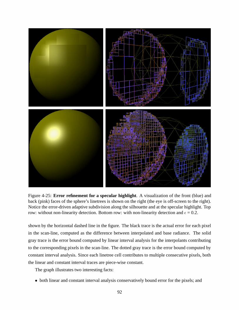
Figure 4-25: Error refinement for a specular highlight. A visualization of the front (blue) andback (pink) faces of the sphere’s linetrees is shown on the right (the eye is off-screen to the right).Notice the error-driven adaptive subdivision along the silhouette and at the specular highlight. Toprow: without non-linearity detection. Bottom row: with non-linearity detection and ε = 0.2.

shown by the horizontal dashed line in the figure. The black trace is the actual error for each pixel

in the scan-line, computed as the difference between interpolated and base radiance. The solid

gray trace is the error bound computed by linear interval analysis for the interpolants contributing

to the corresponding pixels in the scan-line. The dotted gray trace is the error bound computed by

constant interval analysis. Since each linetree cell contributes to multiple consecutive pixels, both

the linear and constant interval traces are piece-wise constant.

The graph illustrates two interesting facts:

• both linear and constant interval analysis conservatively bound error for the pixels; and

92

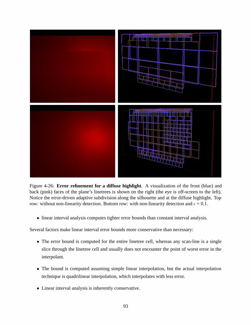
Figure 4-26: Error refinement for a diffuse highlight. A visualization of the front (blue) andback (pink) faces of the plane’s linetrees is shown on the right (the eye is off-screen to the left).Notice the error-driven adaptive subdivision along the silhouette and at the diffuse highlight. Toprow: without non-linearity detection. Bottom row: with non-linearity detection and ε = 0.1.

• linear interval analysis computes tighter error bounds than constant interval analysis.

Several factors make linear interval error bounds more conservative than necessary:

• The error bound is computed for the entire linetree cell, whereas any scan-line is a single

slice through the linetree cell and usually does not encounter the point of worst error in the

interpolant.

• The bound is computed assuming simple linear interpolation, but the actual interpolation

technique is quadrilinear interpolation, which interpolates with less error.

• Linear interval analysis is inherently conservative.

93

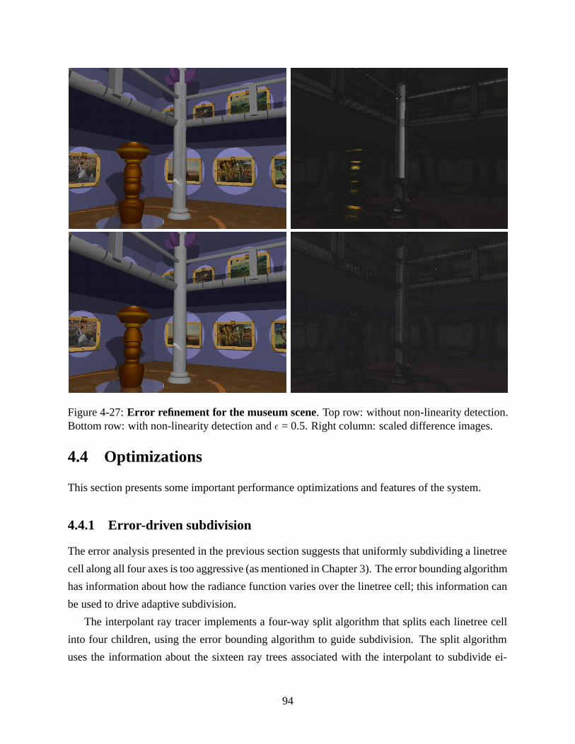
Figure 4-27: Error refinement for the museum scene. Top row: without non-linearity detection.Bottom row: with non-linearity detection and ε = 0.5. Right column: scaled difference images.

4.4 Optimizations

This section presents some important performance optimizations and features of the system.

4.4.1 Error-driven subdivision

The error analysis presented in the previous section suggests that uniformly subdividing a linetree

cell along all four axes is too aggressive (as mentioned in Chapter 3). The error bounding algorithm

has information about how the radiance function varies over the linetree cell; this information can

be used to drive adaptive subdivision.

The interpolant ray tracer implements a four-way split algorithm that splits each linetree cell

into four children, using the error bounding algorithm to guide subdivision. The split algorithm

uses the information about the sixteen ray trees associated with the interpolant to subdivide ei-

94

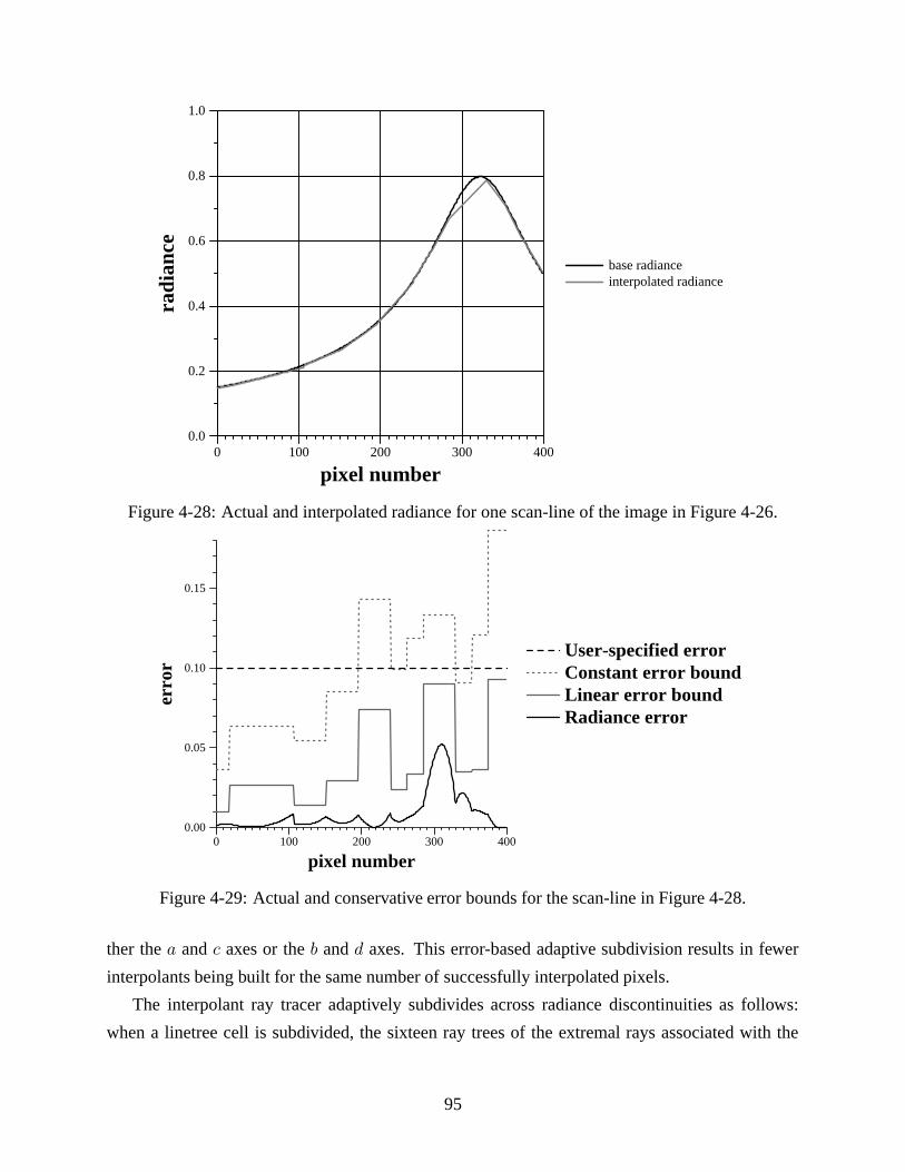
0 100 200 300 400

pixel number

0.0

0.2

0.4

0.6

0.8

1.0

radi

ance

base radianceinterpolated radiance

Figure 4-28: Actual and interpolated radiance for one scan-line of the image in Figure 4-26.

0 100 200 300 400

pixel number

0.00

0.05

0.10

0.15

erro

r

User-specified errorConstant error boundLinear error boundRadiance error

Figure 4-29: Actual and conservative error bounds for the scan-line in Figure 4-28.

ther the a and c axes or the b and d axes. This error-based adaptive subdivision results in fewer

interpolants being built for the same number of successfully interpolated pixels.

The interpolant ray tracer adaptively subdivides across radiance discontinuities as follows:

when a linetree cell is subdivided, the sixteen ray trees of the extremal rays associated with the

95

cell are considered. If all sixteen ray trees are the same, the cell is simply subdivided on the basis

of aspect ratio. However, if the sixteen ray trees differ, the algorithm splits the cell on that pair of

axes that maintains the maximum coherence. Coherence is destroyed if splitting an axis spreads

rays with the same position-independent ray tree to different children. When picking the pair of

axes to split, that pair is picked that spreads the least number of ray trees to different children.

For the museum scene, using error-driven subdivision results in a 35% speedup. This is because

maintaining the coherence in a cell results in fewer subdivisions of the linetree for the same image

quality and in turn, results in fewer interpolants being built.

This technique could also be applied to adaptive subdivision across regions with non-linear

radiance variation. The linear interval terms Li constructed by the error bounding algorithm rep-

resent the variation in the corresponding axis i ∈ {a, b, c, d}. The pair of axes that has the largest

Li’s would be selected for subdivision.

4.4.2 Unique ray trees

Storing radiance samples and their associated ray trees could result in substantial memory usage.

However, all valid interpolants and a large number of invalid interpolants are associated with sim-

ilar ray trees. Therefore, the interpolant ray tracer uses hash tables to avoid storing duplicate ray

trees, resulting in substantial memory savings.

4.4.3 Textures

The interpolant ray tracer supports textured objects by separating the texture coordinate computa-

tion from texture lookup. Texture coordinates and incoming radiance at the textured surface are

both quadrilinearly interpolated. In general, multiple textures may contribute to the radiance of an

interpolant. The texture coordinates of every contributing texture, and the appropriate weighting

of each texture by the incoming radiance are recorded in the interpolant for each of the sixteen

extremal rays and are separately interpolated. For reflected textures, an additional ray must be shot

for each contributing texture from the point of reflection to compute the texture coordinates used

in interpolation.

4.5 Extensions to scene and lighting models

The error bounding algorithm is based on certain assumptions about the scene model and light-

ing model supported by the interpolant ray tracer, as described in Section 4.1.2. The interpolant

96

ray tracer can be applied to more general scenes and lighting models, but in these cases the error

bounding algorithm presented in this chapter does not guarantee that error is bounded. It is inter-

esting to consider the difficulty of extending the error bounding algorithm to support more general

models. A few possible extensions are discussed here.

• Parametric surfaces: It would be useful for the ray tracer to support a more general model

of surfaces, such as bicubic spline patches. Support for non-convex surfaces would also

be useful. In both cases the non-linear variations in radiance can be bounded by applying

the linear interval techniques from this chapter. The intersection and normal for parametric

surfaces can be bounded by using root finding on linear intervals [Han75]. The assumption

of convexity is more difficult to eliminate because it is used in various ways during the

detection of discontinuities. One possibility is to use interval-based techniques to bound the

degree to which a surface is non-convex; another is to bound the surface on the inside and

outside using convex surfaces.

• Generalized shading model: The interpolant ray tracer uses the isotropic Ward model for

local shading, and the Whitted ray tracing model for global illumination. The techniques

discussed in this chapter can be extended to other local shading models such as non-isotropic

Ward [War92], Cook-Torrance [CT82], He [HTSG91], and others [Gla95, WC88]. Only

the linear interval techniques that identify non-linear radiance variations would need to be

modified. Because these linear interval techniques are very general, application to these

other models should be straightforward.

It would be desirable for the ray tracer to include a global illumination model that supports

more generalized light transport paths such as diffuse inter-reflections and caustics. Diffuse

inter-reflections often produce a smoother distribution of light energy within the scene, so

one would expect radiance interpolation to be more successful. Techniques for bounding

error in radiosity systems [LSG94] may be useful. Bounding error from caustics is more

difficult.

• Textures: Using the existing algorithm, the system can be extended straightforwardly to

support texturing of the specular or reflective coefficients of surfaces. Bump maps [Bli78]

could also be supported without difficulty. Some more sophisticated texturing techniques

that change object geometry, such as displacement maps [Coo84], are more difficult to sup-

port.

• Light sources: Support for area light sources or other clusters of lights would be useful. Like

97

diffuse inter-reflections, area light sources are expected to make interpolation more success-

ful. However, for the purposes of bounding error, it is important to accurately characterize

the partial occlusion of area light sources and clustered light sources. This characterization

is well known to be difficult [CW93, SP94].

Chapter 8 further discusses how the interpolant ray tracer can be extended to address each of

these limitations.

4.6 Discussion: error approximation

Another approach that can be used to detect non-linear radiance variations in place of interval

arithmetic is error approximation. While error approximation can occasionally result in erroneous

interpolation, it can be used to produce good image quality at a lower cost. In [BDT98], I pre-

sented an algorithm that uses error approximation to guide sampling. This algorithm computes

the components of the second-order Taylor expansion of the radiance function around the center

of the linetree cell. These second-order terms of the Taylor expansion, which are the interpolation

error at the center of the cell, are used to estimate error over the rest of the linetree cell. This

technique is effective because the maximum interpolation error typically occurs near the center of

the linetree cell. By measuring interpolation error at the center of the linetree cell, this technique

typically produces a more accurate estimate of error than interval arithmetic does, though it is not

conservative.

98

Chapter 5

Accelerating visibility

Using interpolants to approximate radiance eliminates a significant fraction of the shading compu-

tations and their associated intersections invoked by a ray tracer; however, the number of intersec-

tions computed for determining visibility remains the same. Once interpolants accelerate shading,

the cost of rendering a frame is dominated by the following three operations:

• determining visibility at each pixel—constructing a ray from the eye through the pixel and

intersecting that ray with the scene to find the closest visible object,

• for pixels that can be interpolated, computing the 4D intercepts for the ray and evaluating

radiance by quadrilinear interpolation, and

• for pixels that cannot be interpolated (because valid interpolants are unavailable), evaluating

radiance using the base ray tracer.

This chapter presents techniques to accelerate visibility determination and interpolation by further

exploiting temporal and image-space coherence, reducing the cost of these operations.

5.1 Temporal coherence

For complex scenes, determining visibility at each pixel is expensive. However, if multiple frames

of a scene are being rendered from nearby viewpoints, temporal coherence can be exploited to

reduce the cost of determining visibility. For small changes in the viewpoint, objects that are visible

in one frame are often visible in subsequent frames. This temporal coherence occurs because eye

rays from the new viewpoint are close (in ray space) to eye rays from the previous viewpoint.

For the same reason, linetree cells that contribute to one frame typically contribute to subsequent

99

frames. This section presents a reprojection algorithm that exploits this temporal coherence to

accelerate visibility determination, while guaranteeing that the correct visible surface is always

assigned to each pixel.

Consider a pixel that is rendered in one frame using a particular interpolant; the linetree cell

for the interpolant is said to coverthe pixel in that frame. A linetree cell typically covers a number

of adjacent pixels on the image plane; this set of pixels can be computed by a simple geometric

projection. When rendering a series of frames, this property is used to identify pixels covered by

linetree cells. For each frame, linetree cells that contributed to the previous frame are reprojected

to the current viewpoint to determine which pixels are covered by these cells.

Using reprojection to determine visibility accelerates rendering in the following way. If a pixel

in the new frame is covered by a linetree cell, it is not necessary to compute visibility or shading

for that pixel: the radiance of the pixel can be computed directly from the interpolant associated

with that cell. Since a linetree cell typically covers multiple pixels, the cost of reprojecting the

cell is amortized across many pixels. Reprojection also enables scan-line interpolation, further

accelerating rendering (see Section 5.2).

There are two important issues to be considered:

1. how to reproject linetree cells efficiently, and

2. how to guarantee that a cell is reprojected to a pixel only if it covers that pixel in the new

frame. Note that the reprojection algorithm is conservative since it never incorrectly assigns

a linetree to a pixel.

These two issues are discussed in detail in the following sections: Section 5.1.1 shows how linetree

cells can be efficiently reprojected using the graphics hardware, and Section 5.1.2 describes how

shaft-culling is used to ensure that the correct visible surface is always assigned to each pixel.

5.1.1 Reprojecting linetrees

First, we consider reprojecting linetrees in 2D. In 2D, each linetree cell represents all the rays that

enter its front line segment and leave its back line segment. For a given viewpoint, a cell covers

some (possibly empty) set of pixels; the rays from the viewpoint through these pixels are a subset

of the rays represented by the linetree cell. Given a viewpoint, the pixels covered by a linetree cell

and their corresponding rays can be found efficiently as shown below.

On the left in Figure 5-1, a linetree cell, L, of an object is shown; the front segment of L is

shown in light gray and its back segment is shown in black. In this frame, the viewpoint is at the

point eye. A ray from the viewpoint that lies in L must intersect both its front and back segment.

100

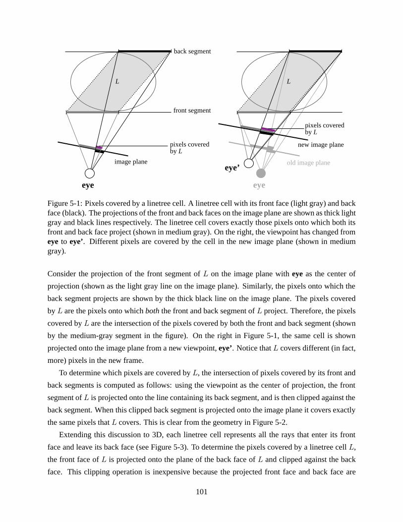
new image plane

eye

eye’

pixels coveredby L

back segment

front segment

image plane

eye

old image plane

L L

pixels coveredby L

Figure 5-1: Pixels covered by a linetree cell. A linetree cell with its front face (light gray) and backface (black). The projections of the front and back faces on the image plane are shown as thick lightgray and black lines respectively. The linetree cell covers exactly those pixels onto which both itsfront and back face project (shown in medium gray). On the right, the viewpoint has changed fromeye to eye’ . Different pixels are covered by the cell in the new image plane (shown in mediumgray).

Consider the projection of the front segment of L on the image plane with eye as the center of

projection (shown as the light gray line on the image plane). Similarly, the pixels onto which the

back segment projects are shown by the thick black line on the image plane. The pixels covered

by L are the pixels onto which boththe front and back segment of L project. Therefore, the pixels

covered by L are the intersection of the pixels covered by both the front and back segment (shown

by the medium-gray segment in the figure). On the right in Figure 5-1, the same cell is shown

projected onto the image plane from a new viewpoint, eye’ . Notice that L covers different (in fact,

more) pixels in the new frame.

To determine which pixels are covered by L, the intersection of pixels covered by its front and

back segments is computed as follows: using the viewpoint as the center of projection, the front

segment of L is projected onto the line containing its back segment, and is then clipped against the

back segment. When this clipped back segment is projected onto the image plane it covers exactly

the same pixels that L covers. This is clear from the geometry in Figure 5-2.

Extending this discussion to 3D, each linetree cell represents all the rays that enter its front

face and leave its back face (see Figure 5-3). To determine the pixels covered by a linetree cell L,

the front face of L is projected onto the plane of the back face of L and clipped against the back

face. This clipping operation is inexpensive because the projected front face and back face are

101

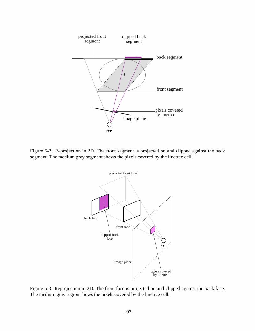
pixels coveredby linetree

back segment

front segment

image plane

eye

projected frontsegment

clipped backsegment

L

Figure 5-2: Reprojection in 2D. The front segment is projected on and clipped against the backsegment. The medium gray segment shows the pixels covered by the linetree cell.

front face

back face

eye

projected front face

clipped backface

pixels coveredby linetree

image plane

Figure 5-3: Reprojection in 3D. The front face is projected on and clipped against the back face.The medium gray region shows the pixels covered by the linetree cell.

102

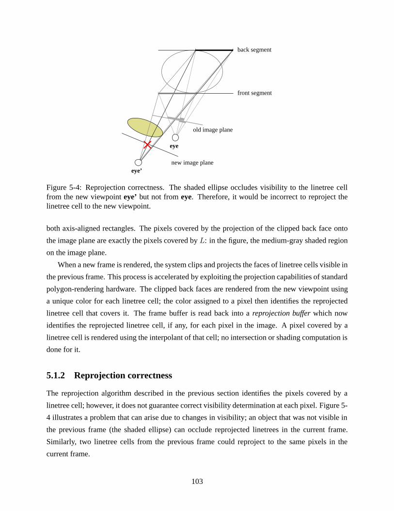
back segment

front segment

old image plane

eye

eye’new image plane

Figure 5-4: Reprojection correctness. The shaded ellipse occludes visibility to the linetree cellfrom the new viewpoint eye’ but not from eye. Therefore, it would be incorrect to reproject thelinetree cell to the new viewpoint.

both axis-aligned rectangles. The pixels covered by the projection of the clipped back face onto

the image plane are exactly the pixels covered by L: in the figure, the medium-gray shaded region

on the image plane.

When a new frame is rendered, the system clips and projects the faces of linetree cells visible in

the previous frame. This process is accelerated by exploiting the projection capabilities of standard

polygon-rendering hardware. The clipped back faces are rendered from the new viewpoint using

a unique color for each linetree cell; the color assigned to a pixel then identifies the reprojected

linetree cell that covers it. The frame buffer is read back into a reprojection bufferwhich now

identifies the reprojected linetree cell, if any, for each pixel in the image. A pixel covered by a

linetree cell is rendered using the interpolant of that cell; no intersection or shading computation is

done for it.

5.1.2 Reprojection correctness

The reprojection algorithm described in the previous section identifies the pixels covered by a

linetree cell; however, it does not guarantee correct visibility determination at each pixel. Figure 5-

4 illustrates a problem that can arise due to changes in visibility; an object that was not visible in

the previous frame (the shaded ellipse) can occlude reprojected linetrees in the current frame.

Similarly, two linetree cells from the previous frame could reproject to the same pixels in the

current frame.

103

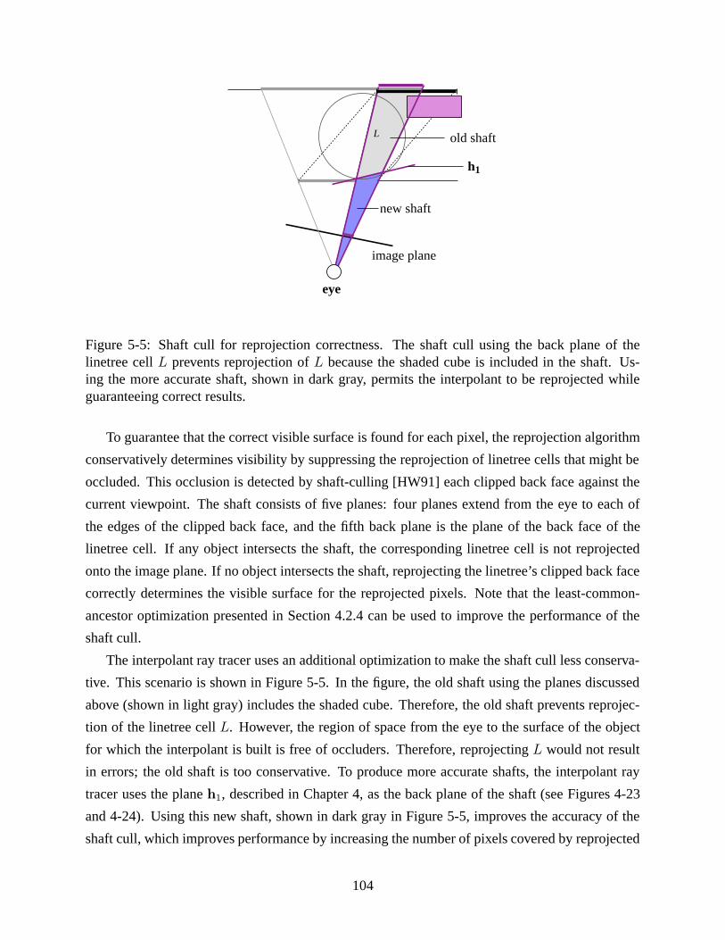
image plane

eye

L

new shaft

old shaft

h1

Figure 5-5: Shaft cull for reprojection correctness. The shaft cull using the back plane of thelinetree cell L prevents reprojection of L because the shaded cube is included in the shaft. Us-ing the more accurate shaft, shown in dark gray, permits the interpolant to be reprojected whileguaranteeing correct results.

To guarantee that the correct visible surface is found for each pixel, the reprojection algorithm

conservatively determines visibility by suppressing the reprojection of linetree cells that might be

occluded. This occlusion is detected by shaft-culling [HW91] each clipped back face against the

current viewpoint. The shaft consists of five planes: four planes extend from the eye to each of

the edges of the clipped back face, and the fifth back plane is the plane of the back face of the

linetree cell. If any object intersects the shaft, the corresponding linetree cell is not reprojected

onto the image plane. If no object intersects the shaft, reprojecting the linetree’s clipped back face

correctly determines the visible surface for the reprojected pixels. Note that the least-common-

ancestor optimization presented in Section 4.2.4 can be used to improve the performance of the

shaft cull.

The interpolant ray tracer uses an additional optimization to make the shaft cull less conserva-

tive. This scenario is shown in Figure 5-5. In the figure, the old shaft using the planes discussed

above (shown in light gray) includes the shaded cube. Therefore, the old shaft prevents reprojec-

tion of the linetree cell L. However, the region of space from the eye to the surface of the object

for which the interpolant is built is free of occluders. Therefore, reprojecting L would not result

in errors; the old shaft is too conservative. To produce more accurate shafts, the interpolant ray

tracer uses the plane h1, described in Chapter 4, as the back plane of the shaft (see Figures 4-23

and 4-24). Using this new shaft, shown in dark gray in Figure 5-5, improves the accuracy of the

shaft cull, which improves performance by increasing the number of pixels covered by reprojected

104

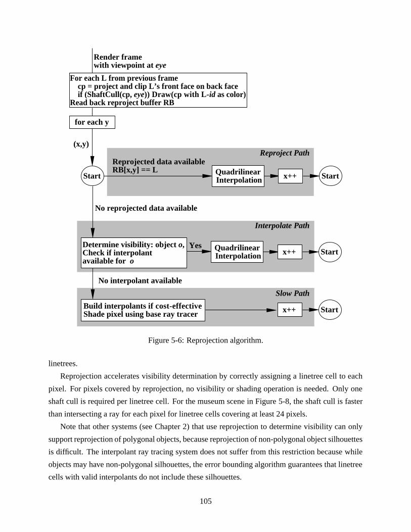
(x,y)

Reprojected data availableRB[x,y] == L

Reproject Path

No reprojected data available

Interpolate Path

Start

Slow Path

Render frame with viewpoint at eye

Yes

No interpolant available

Build interpolants if cost-effectiveShade pixel using base ray tracer

Start

Determine visibility: object o,Check if interpolantavailable for o

Quadrilinear Interpolation x++

StartQuadrilinear Interpolation x++

Startx++

for each y

For each L from previous frame cp = project and clip L’s front face on back face if (ShaftCull(cp, eye)) Draw(cp with L-id as color)Read back reproject buffer RB

Figure 5-6: Reprojection algorithm.

linetrees.

Reprojection accelerates visibility determination by correctly assigning a linetree cell to each

pixel. For pixels covered by reprojection, no visibility or shading operation is needed. Only one

shaft cull is required per linetree cell. For the museum scene in Figure 5-8, the shaft cull is faster

than intersecting a ray for each pixel for linetree cells covering at least 24 pixels.

Note that other systems (see Chapter 2) that use reprojection to determine visibility can only

support reprojection of polygonal objects, because reprojection of non-polygonal object silhouettes

is difficult. The interpolant ray tracing system does not suffer from this restriction because while

objects may have non-polygonal silhouettes, the error bounding algorithm guarantees that linetree

cells with valid interpolants do not include these silhouettes.

105

The rendering algorithm with reprojection is summarized in Figure 5-6. Before a frame is ren-

dered, all linetree cells that contribute to the previous frame are clipped and shaft-culled against the

new viewpoint, obtaining a list of conservatively unoccluded linetree cells. These cells are repro-

jected using the polygon-rendering hardware. The frame buffer is read back into the reprojection

buffer (RB) which identifies the linetree cell (if any) that covers each pixel in the image. The frame

is rendered using the reprojection buffer to determine visibility when possible. For each pixel, the

reprojection buffer is checked for the availability of a reprojected linetree cell. If such a cell ex-

ists, radiance for the pixel is quadrilinearly interpolated using the linetree cell. If no reprojected

linetree cell is available, visibility at the pixel is determined by tracing the corresponding eye ray

through the scene. If the closest visible object o along the eye ray has a valid interpolant for the

eye ray, radiance for that pixel is quadrilinearly interpolated; this is the interpolate pathreferred to

in Section 1.5.1. If no interpolant is available for the pixel, the eye ray is ray traced using the base

ray tracer: the slow path. On the slow path, interpolants are built only if deemed cost-effective (see

Section 3.5.4).

5.1.3 Optimizations: adaptive shaft-culling

The reprojection algorithm shaft-culls linetree cells from the previous frame. If an object is com-

pletely visible, it is wasteful to shaft-cull each of its linetree cells separately. This is also true

if some significant number of linetree cells associated with the object are unoccluded. To avoid

redundant work, the interpolant ray tracer uses clustering to amortize the cost of shaft-culling over

multiple linetree cells. The algorithm clusters all the linetree cells of an object and shaft-culls the

cluster. If the shaft cull succeeds, a significant performance improvement is achieved by eliminat-

ing the shaft cull for each individual cell. If the shaft cull fails, the cluster is recursively subdivided

spatially along its two non-principal axes, and the four resulting clusters are shaft-culled. This

recursive subdivision is repeated until the cluster size is reduced to a single linetree cell. For the

museum scene shown in Figure 5-8, clustering decreases the number of shaft culls by about a factor

of four.

Another problem with the reprojection algorithm is that it could be too conservative because

large linetree cells that are only partially occluded by some occluder are not reprojected. To address

this problem, when the interpolant ray tracer subdivides a cluster down to a single linetree cell, it

uses a cost model similar to that used for subdividing linetrees (see Section 3.5.4) to compute the

number of pixels covered by the single cell. If the number of pixels covered by the cell is significant

(at least 24 for the museum scene in Figure 5-8), the linetree cell in turn is recursively subdivided

and shaft-culled. The portions of the faces that are not blocked are then reprojected. This adaptive

106

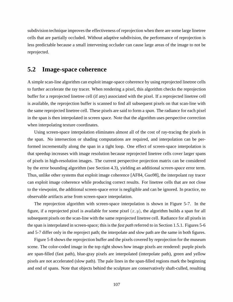
subdivision technique improves the effectiveness of reprojection when there are some large linetree

cells that are partially occluded. Without adaptive subdivision, the performance of reprojection is

less predictable because a small intervening occluder can cause large areas of the image to not be

reprojected.

5.2 Image-space coherence

A simple scan-line algorithm can exploit image-space coherence by using reprojected linetree cells

to further accelerate the ray tracer. When rendering a pixel, this algorithm checks the reprojection

buffer for a reprojected linetree cell (if any) associated with the pixel. If a reprojected linetree cell

is available, the reprojection buffer is scanned to find all subsequent pixels on that scan-line with

the same reprojected linetree cell. These pixels are said to form a span. The radiance for each pixel

in the span is then interpolated in screen space. Note that the algorithm uses perspective correction

when interpolating texture coordinates.

Using screen-space interpolation eliminates almost all of the cost of ray-tracing the pixels in

the span. No intersection or shading computations are required, and interpolation can be per-

formed incrementally along the span in a tight loop. One effect of screen-space interpolation is

that speedup increases with image resolution because reprojected linetree cells cover larger spans

of pixels in high-resolution images. The current perspective projection matrix can be considered

by the error bounding algorithm (see Section 4.3), yielding an additional screen-spaceerror term.

Thus, unlike other systems that exploit image coherence [AF84, Guo98], the interpolant ray tracer

can exploit image coherence while producing correct results. For linetree cells that are not close

to the viewpoint, the additional screen-space error is negligible and can be ignored. In practice, no

observable artifacts arise from screen-space interpolation.

The reprojection algorithm with screen-space interpolation is shown in Figure 5-7. In the

figure, if a reprojected pixel is available for some pixel (x, y), the algorithm builds a span for all

subsequent pixels on the scan-line with the same reprojected linetree cell. Radiance for all pixels in

the span is interpolated in screen-space; this is the fast pathreferred to in Section 1.5.1. Figures 5-6

and 5-7 differ only in the reproject path; the interpolate and slow path are the same in both figures.

Figure 5-8 shows the reprojection buffer and the pixels covered by reprojection for the museum

scene. The color-coded image in the top right shows how image pixels are rendered: purple pixels

are span-filled (fast path), blue-gray pixels are interpolated (interpolate path), green and yellow

pixels are not accelerated (slow path). The pale lines in the span-filled regions mark the beginning

and end of spans. Note that objects behind the sculpture are conservatively shaft-culled, resulting

107

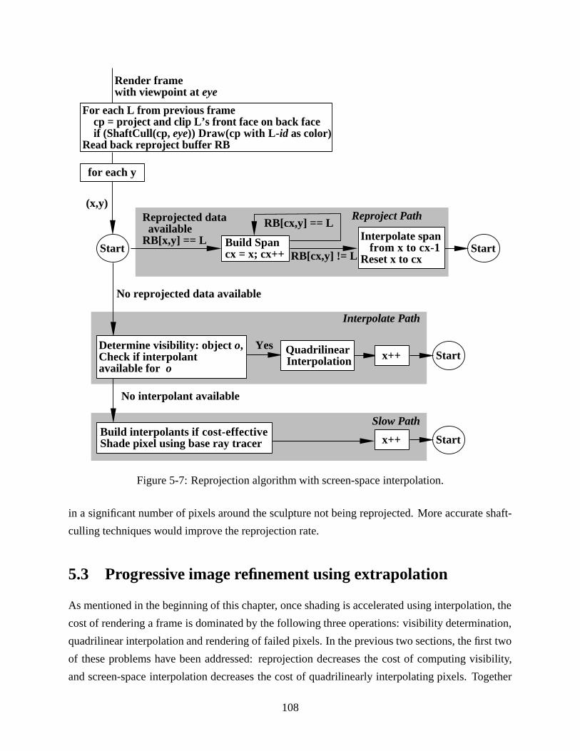
Interpolate span from x to cx-1Reset x to cx

(x,y)

No reprojected data available

Interpolate Path

Start

Slow Path

Render frame with viewpoint at eye

Yes

No interpolant available

Build interpolants if cost-effectiveShade pixel using base ray tracer

Determine visibility: object o,Check if interpolantavailable for o

StartQuadrilinear Interpolation x++

Reprojected data availableRB[x,y] == L

Reproject PathRB[cx,y] == L

RB[cx,y] != LBuild Spancx = x; cx++ Start

Startx++

For each L from previous frame cp = project and clip L’s front face on back face if (ShaftCull(cp, eye)) Draw(cp with L-id as color)Read back reproject buffer RB

for each y

Figure 5-7: Reprojection algorithm with screen-space interpolation.

in a significant number of pixels around the sculpture not being reprojected. More accurate shaft-

culling techniques would improve the reprojection rate.

5.3 Progressive image refinement using extrapolation

As mentioned in the beginning of this chapter, once shading is accelerated using interpolation, the

cost of rendering a frame is dominated by the following three operations: visibility determination,

quadrilinear interpolation and rendering of failed pixels. In the previous two sections, the first two

of these problems have been addressed: reprojection decreases the cost of computing visibility,

and screen-space interpolation decreases the cost of quadrilinearly interpolating pixels. Together

108

Figure 5-8: Reprojection for the museum scene. Top row (left to right): reprojection buffer,color-coded image. Middle row: span-filled pixels, span-filled and interpolated pixels. Bottom:final image.

109

these optimizations enable most pixels to be rendered rapidly. However, rendering pixels that are

neither reprojected nor interpolated (failed pixels) now dominates the time to render a frame. If a

guaranteed rendering frame rate is desired, it is necessary to eliminate the cost of ray tracing the

failed pixels using some approximation for those pixels; however, this approximation cannot be

expected to meet the error guarantees provided by the error bounding algorithm.

In this section, algorithms that approximate radiance for the failed pixels are presented. These

algorithms extrapolate radiance computed for the reprojected or interpolated pixels. The reprojec-

tion algorithm is the same as shown in Figure 5-7; the interpolate and slow path of the algorithm

are replaced by the extrapolation algorithm.

5.3.1 Algorithm 1: Simple extrapolation

The first and fastest extrapolation algorithm renders all the pixels in the scan-line that have a repro-

jected linetree cell available. The pixels that are not reprojected are then filled in by extrapolating

radiance from the reprojected pixels. This algorithm is fast because it fills in the failed pixels with-

out doing any shading or visibility; however, it extrapolates radiance between different objects,

resulting in noticeable visual artifacts such as blurred object edges and color bleeding between

different objects as can be seen in Figure 5-10.

5.3.2 Algorithm 2: Extrapolation with correct visibility

A second extrapolation algorithm uses both reprojection and interpolation to render pixels. This

algorithm renders all the pixels in the scan-line that have a reprojected linetree or have an inter-

polant available. As before, all pixels that have reprojected linetrees are screen-space interpolated.

If a reprojected linetree is not available for the pixel, the algorithm finds the closest visible object

at the pixel. Then, if an interpolant is available, radiance is quadrilinearly interpolated for the

pixel. The remaining failed pixels are filled in by extrapolating radiance from the reprojected or

interpolated pixels. However, since the algorithm computes visibility at each pixel to check for the

availability of a valid interpolant, this visibility information is put to use during extrapolation to

guarantee correct visibility determination at each pixel.

This extrapolation algorithm is shown in Figure 5-9. The algorithm finds the closest two pixels,

p and n, before and after the current pixel, that also intersect the same object. If p and n are

reprojected or interpolated, radiance for all pixels between p and n (including the current pixels)

are extrapolated. If p (or n) is neither reprojected nor interpolated, radiance for p (or n) is evaluated

along the slow path. The radiance for all pixels between p and n is then extrapolated. Note that

110

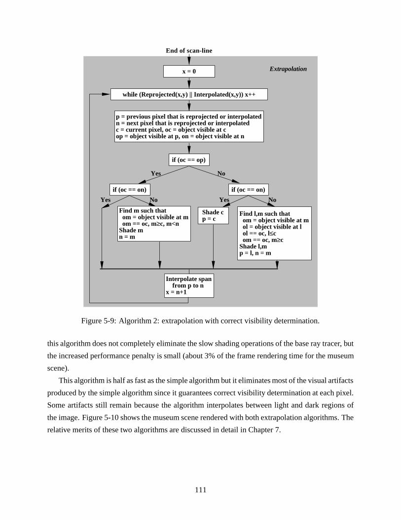
Extrapolation

End of scan-line

x = 0

while (Reprojected(x,y) || Interpolated(x,y)) x++

Yes

Yes

if (oc == on)

No Yes

if (oc == on)

No

if (oc == op)

No

p = previous pixel that is reprojected or interpolatedn = next pixel that is reprojected or interpolatedc = current pixel, oc = object visible at cop = object visible at p, on = object visible at n

Find m such that om = object visible at m om == oc, m≥c, m<nShade mn = m

Shade cp = c

Interpolate span from p to nx = n+1

Find l,m such that om = object visible at m ol = object visible at l ol == oc, l≤c om == oc, m≥cShade l,mp = l, n = m

Figure 5-9: Algorithm 2: extrapolation with correct visibility determination.

this algorithm does not completely eliminate the slow shading operations of the base ray tracer, but

the increased performance penalty is small (about 3% of the frame rendering time for the museum

scene).

This algorithm is half as fast as the simple algorithm but it eliminates most of the visual artifacts

produced by the simple algorithm since it guarantees correct visibility determination at each pixel.

Some artifacts still remain because the algorithm interpolates between light and dark regions of

the image. Figure 5-10 shows the museum scene rendered with both extrapolation algorithms. The

relative merits of these two algorithms are discussed in detail in Chapter 7.

111

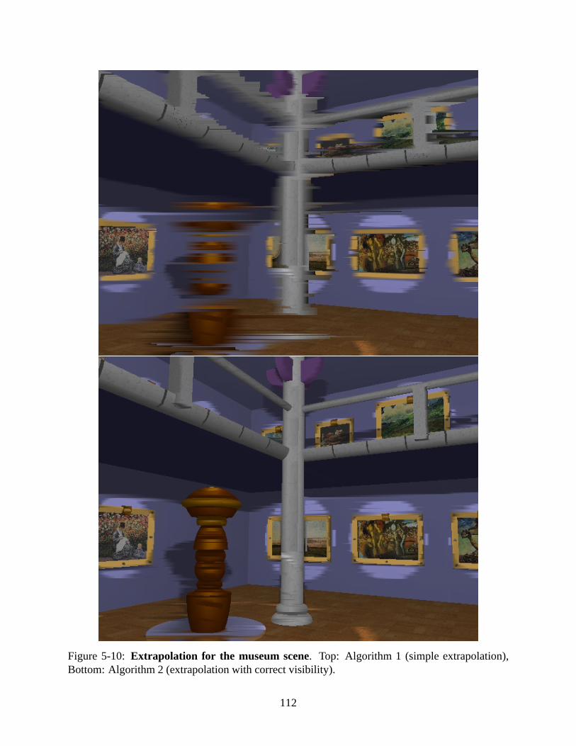
Figure 5-10: Extrapolation for the museum scene. Top: Algorithm 1 (simple extrapolation),Bottom: Algorithm 2 (extrapolation with correct visibility).

112

5.3.3 Algorithms 3 and 4: Progressive refinement

For interactive performance, several complementary techniques can be used to provide the user

with a progressively refined rendered image. The pixels that are not reprojected are filled in by in-

terpolating between reprojected pixels in various ways: the system uses two algorithms to produce

progressively higher image quality than that produced by Algorithm 1 (the simple extrapolation

algorithm), while being faster than Algorithm 2 (the extrapolation algorithm that guarantees cor-

rect visibility). Both these algorithms are faster because they use a binary search [CLR90] of the

scan-line to find the previous and next pixels p and n described in Figure 5-9. However, neither of

these algorithms guarantee correct visibility, since the binary search might miss small intermediate

objects in the scan-line.

Algorithm 3: Progressive refinement with visibility check. This algorithm finds p and n using

a binary search of the scan-line such that the object visible at p and n are the same. This test

is similar to that done by the Algorithm 2, except that correct visibility is not guaranteed. If the

maximum length of a span is not restricted, this algorithm produces results that are only slightly

better (visually) than Algorithm 1. However, if the maximum length of a span is restricted, the

results produced are as shown in Figure 5-11. (In the figure, the maximum span length is set to

20.) Note that there are some visual artifacts due to erroneous interpolation across shadows (as in

Algorithm 2) and artifacts due to incorrect visibility determination, which are particularly visible

at the frames of the paintings. However, the results are visually similar to those produced by

Algorithm 2, while being computed much faster.

Algorithm 4: Progressive refinement with ray tree comparisons. This algorithm uses binary

search to find the previous and next pixels p and n such that these pixels have the same ray tree

as the current pixel. Comparing ray trees causes increased subdivision of the scan-line when

compared to Algorithm 3, but also produces substantially improved image quality as shown in

Figure 5-11. The images produced using this algorithm are often nearly indistinguishable from the

images using the interpolant ray tracer with error guarantees, though some visual artifacts are still

visible on the sculpture. This algorithm uses the fact that both reprojection and interpolation look

up interpolants that have ray trees associated with them; these ray trees are used to obtain improved

image quality.

113

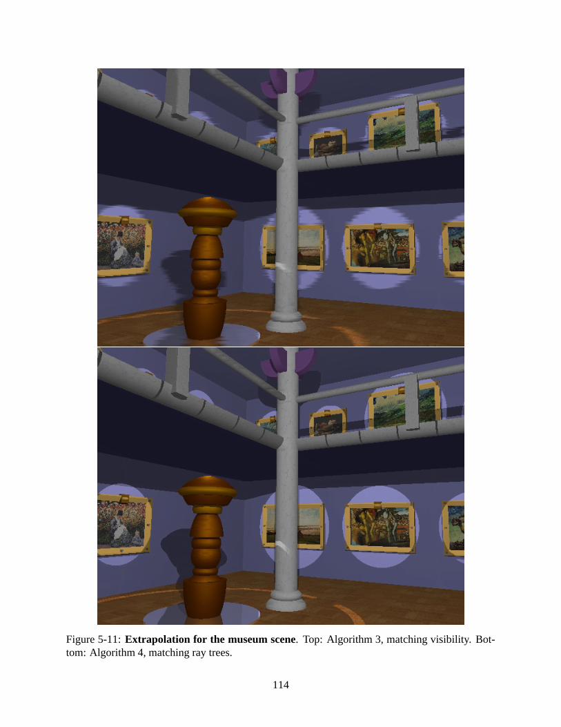
Figure 5-11: Extrapolation for the museum scene. Top: Algorithm 3, matching visibility. Bot-tom: Algorithm 4, matching ray trees.

114

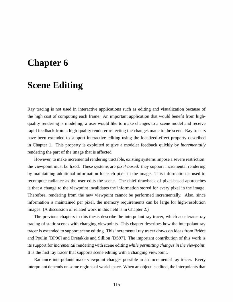
Chapter 6

Scene Editing

Ray tracing is not used in interactive applications such as editing and visualization because of

the high cost of computing each frame. An important application that would benefit from high-

quality rendering is modeling; a user would like to make changes to a scene model and receive

rapid feedback from a high-quality renderer reflecting the changes made to the scene. Ray tracers

have been extended to support interactive editing using the localized-effect property described

in Chapter 1. This property is exploited to give a modeler feedback quickly by incrementally

rendering the part of the image that is affected.

However, to make incremental rendering tractable, existing systems impose a severe restriction:

the viewpoint must be fixed. These systems are pixel-based: they support incremental rendering

by maintaining additional information for each pixel in the image. This information is used to

recompute radiance as the user edits the scene. The chief drawback of pixel-based approaches

is that a change to the viewpoint invalidates the information stored for every pixel in the image.

Therefore, rendering from the new viewpoint cannot be performed incrementally. Also, since

information is maintained per pixel, the memory requirements can be large for high-resolution

images. (A discussion of related work in this field is in Chapter 2.)

The previous chapters in this thesis describe the interpolant ray tracer, which accelerates ray

tracing of static scenes with changing viewpoints. This chapter describes how the interpolant ray

tracer is extended to support scene editing. This incremental ray tracer draws on ideas from Briere

and Poulin [BP96] and Dretakkis and Sillion [DS97]. The important contribution of this work is

its support for incrementalrendering with scene editing while permitting changes in the viewpoint.

It is the first ray tracer that supports scene editing with a changing viewpoint.

Radiance interpolants make viewpoint changes possible in an incremental ray tracer. Every

interpolant depends on some regions of world space. When an object is edited, the interpolants that

115

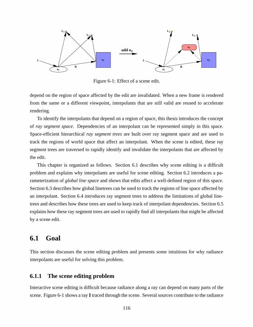
I

R

L1

o1

o2

L2

add o3

I

R

L1

o1

o2

o3

L2

Figure 6-1: Effect of a scene edit.

depend on the region of space affected by the edit are invalidated. When a new frame is rendered

from the same or a different viewpoint, interpolants that are still valid are reused to accelerate

rendering.

To identify the interpolants that depend on a region of space, this thesis introduces the concept

of ray segment space. Dependencies of an interpolant can be represented simply in this space.

Space-efficient hierarchical ray segment treesare built over ray segment space and are used to

track the regions of world space that affect an interpolant. When the scene is edited, these ray

segment trees are traversed to rapidly identify and invalidate the interpolants that are affected by

the edit.

This chapter is organized as follows. Section 6.1 describes why scene editing is a difficult

problem and explains why interpolants are useful for scene editing. Section 6.2 introduces a pa-

rameterization of global line spaceand shows that edits affect a well-defined region of this space.

Section 6.3 describes how global linetrees can be used to track the regions of line space affected by

an interpolant. Section 6.4 introduces ray segment trees to address the limitations of global line-

trees and describes how these trees are used to keep track of interpolant dependencies. Section 6.5

explains how these ray segment trees are used to rapidly find all interpolants that might be affected

by a scene edit.

6.1 Goal

This section discusses the scene editing problem and presents some intuitions for why radiance

interpolants are useful for solving this problem.

6.1.1 The scene editing problem

Interactive scene editing is difficult because radiance along a ray can depend on many parts of the

scene. Figure 6-1 shows a ray I traced through the scene. Several sources contribute to the radiance

116

along I: the lights L1 and L2 contribute to radiance directly, and also indirectly through a reflection

R. Various edits to this scene will change radiance along I. For example, if o2 were deleted, the

radiance along R would change, and indirectly the radiance along I would change. Recall that

each ray has an associated ray tree (see Chapter 4). When an object o is edited, every ray whose

ray tree has o in it could be affected by the edit. Therefore, finding the rays affected by some edits

is straightforward: the affected rays are those whose ray trees mention the edited object.

However, updating rays whose ray trees mention the edited object is not sufficient for all edits.

For example, if o3 were added (as shown in the figure), the radiance along R would change since L1

would become occluded; this would change the radiance along I. Also, L2 would become occluded

directly along I. Thus, even though o3 does not appear in the ray tree for I, the scene edit makes o3

affect the radiance along I. In general, a scene edit affects a ray I if some ray in the ray tree of I

passes through the region of world space affected by the edit. In the figure, the ray from o2 to light

L1 passes through the region of space affected by the edit (the volume of o3).

To make the incremental ray tracer work well, it must address two goals:

• Correctness: All rays affected by a scene edit must be identified and updated; otherwise,

the image rendered will be incorrect. However, some unaffected rays could also be conser-

vatively flagged for update.

• Efficiency: For efficiency, the system should accuratelyidentify the affected rays. When

possible, the system should avoid updating rays that are not affected by the edit, because

these updates are wasted computation.

6.1.2 Edits supported

The difficulty of supporting incremental rendering with scene editing depends on the kinds of edits

allowed. There are several kinds of scene edits of interest for incremental ray tracing [BP96],

which can be categorized usefully as follows:

• attribute changes, which include changes to the material properties of objects: for example,

diffuse color, specular color, diffuse and specular coefficients, and reflective and refractive

coefficients;

• geometry changes, which include adding, deleting, and moving objects;

• changes in viewpoint; and

• changes in lighting.

117

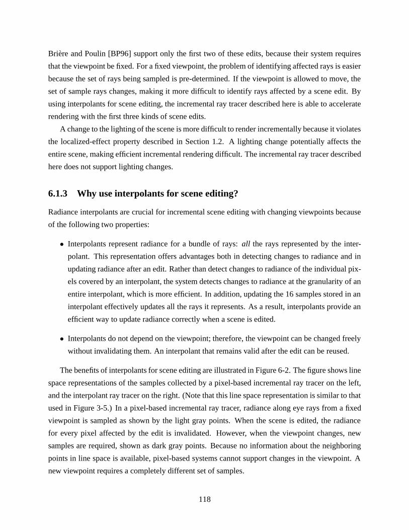
Briere and Poulin [BP96] support only the first two of these edits, because their system requires

that the viewpoint be fixed. For a fixed viewpoint, the problem of identifying affected rays is easier

because the set of rays being sampled is pre-determined. If the viewpoint is allowed to move, the

set of sample rays changes, making it more difficult to identify rays affected by a scene edit. By

using interpolants for scene editing, the incremental ray tracer described here is able to accelerate

rendering with the first three kinds of scene edits.

A change to the lighting of the scene is more difficult to render incrementally because it violates

the localized-effect property described in Section 1.2. A lighting change potentially affects the

entire scene, making efficient incremental rendering difficult. The incremental ray tracer described

here does not support lighting changes.

6.1.3 Why use interpolants for scene editing?

Radiance interpolants are crucial for incremental scene editing with changing viewpoints because

of the following two properties:

• Interpolants represent radiance for a bundle of rays: all the rays represented by the inter-

polant. This representation offers advantages both in detecting changes to radiance and in

updating radiance after an edit. Rather than detect changes to radiance of the individual pix-

els covered by an interpolant, the system detects changes to radiance at the granularity of an

entire interpolant, which is more efficient. In addition, updating the 16 samples stored in an

interpolant effectively updates all the rays it represents. As a result, interpolants provide an

efficient way to update radiance correctly when a scene is edited.

• Interpolants do not depend on the viewpoint; therefore, the viewpoint can be changed freely

without invalidating them. An interpolant that remains valid after the edit can be reused.

The benefits of interpolants for scene editing are illustrated in Figure 6-2. The figure shows line

space representations of the samples collected by a pixel-based incremental ray tracer on the left,

and the interpolant ray tracer on the right. (Note that this line space representation is similar to that

used in Figure 3-5.) In a pixel-based incremental ray tracer, radiance along eye rays from a fixed

viewpoint is sampled as shown by the light gray points. When the scene is edited, the radiance

for every pixel affected by the edit is invalidated. However, when the viewpoint changes, new

samples are required, shown as dark gray points. Because no information about the neighboring

points in line space is available, pixel-based systems cannot support changes in the viewpoint. A

new viewpoint requires a completely different set of samples.

118

s

t

pixel−basedray tracer

s

t

interpolantray tracer

frame 1frame 2

interpolant

Figure 6-2: Interpolants for editing.

The interpolant approach builds interpolants that represent radiance for regions of line space,

independently of the viewpoint (as shown by the rectangles in the figure). Therefore, when the

viewpoint changes, interpolants can be reused. When the scene is edited, affected interpolants are

updated, which effectively updates radiance of all rays represented by the interpolant.

6.2 Ray dependencies

This section describes how to identify the rays affected by an object edit. First, a global four-

dimensional parameterization is presented of all rays intersecting the scene. When an object is

edited, a portion of this global line spaceis affected. Conservatively, the radiance of rays in this

portion of global line space should be recomputed after the edit.

6.2.1 Global line space parameterization

Global line spaceis the space of all directed lines that intersect the scene. In Chapter 3, an object-

space four-dimensional parameterization of rays is presented. A similar parameterization is used

for rays intersecting the scene, except that the face pairs (as shown in Figure 3-3) surround the

entire scene, and w× l×h is the size of the bounding box of the scene. As explained in Chapter 3,

every ray intersecting the scene is associated with a face pair, and the ray is parameterized by the

four intercepts it makes with the two parallel faces of the face pair. Note that per-object line space

119

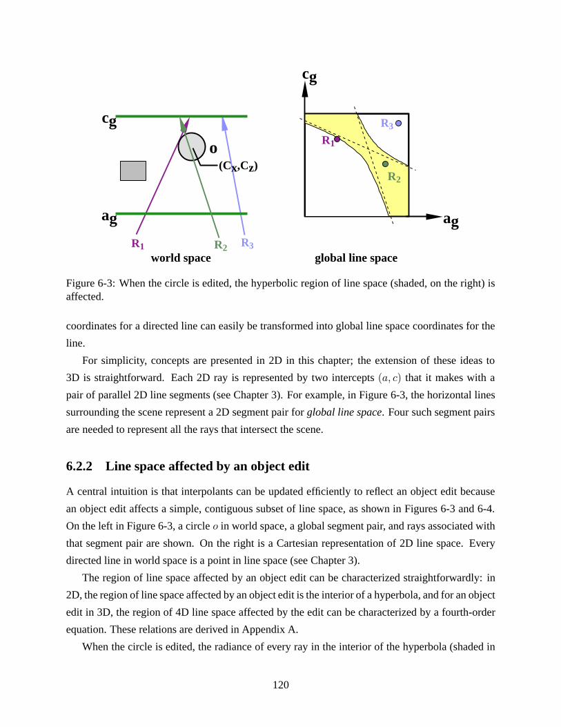
R1 R2 R3

ag

cg

R3

R2

R1

world space global line space

ag

cg

o(Cx,Cz)

Figure 6-3: When the circle is edited, the hyperbolic region of line space (shaded, on the right) isaffected.

coordinates for a directed line can easily be transformed into global line space coordinates for the

line.

For simplicity, concepts are presented in 2D in this chapter; the extension of these ideas to

3D is straightforward. Each 2D ray is represented by two intercepts (a, c) that it makes with a

pair of parallel 2D line segments (see Chapter 3). For example, in Figure 6-3, the horizontal lines

surrounding the scene represent a 2D segment pair for global line space. Four such segment pairs

are needed to represent all the rays that intersect the scene.

6.2.2 Line space affected by an object edit

A central intuition is that interpolants can be updated efficiently to reflect an object edit because

an object edit affects a simple, contiguous subset of line space, as shown in Figures 6-3 and 6-4.

On the left in Figure 6-3, a circle o in world space, a global segment pair, and rays associated with

that segment pair are shown. On the right is a Cartesian representation of 2D line space. Every

directed line in world space is a point in line space (see Chapter 3).

The region of line space affected by an object edit can be characterized straightforwardly: in

2D, the region of line space affected by an object edit is the interior of a hyperbola, and for an object

edit in 3D, the region of 4D line space affected by the edit can be characterized by a fourth-order

equation. These relations are derived in Appendix A.

When the circle is edited, the radiance of every ray in the interior of the hyperbola (shaded in

120

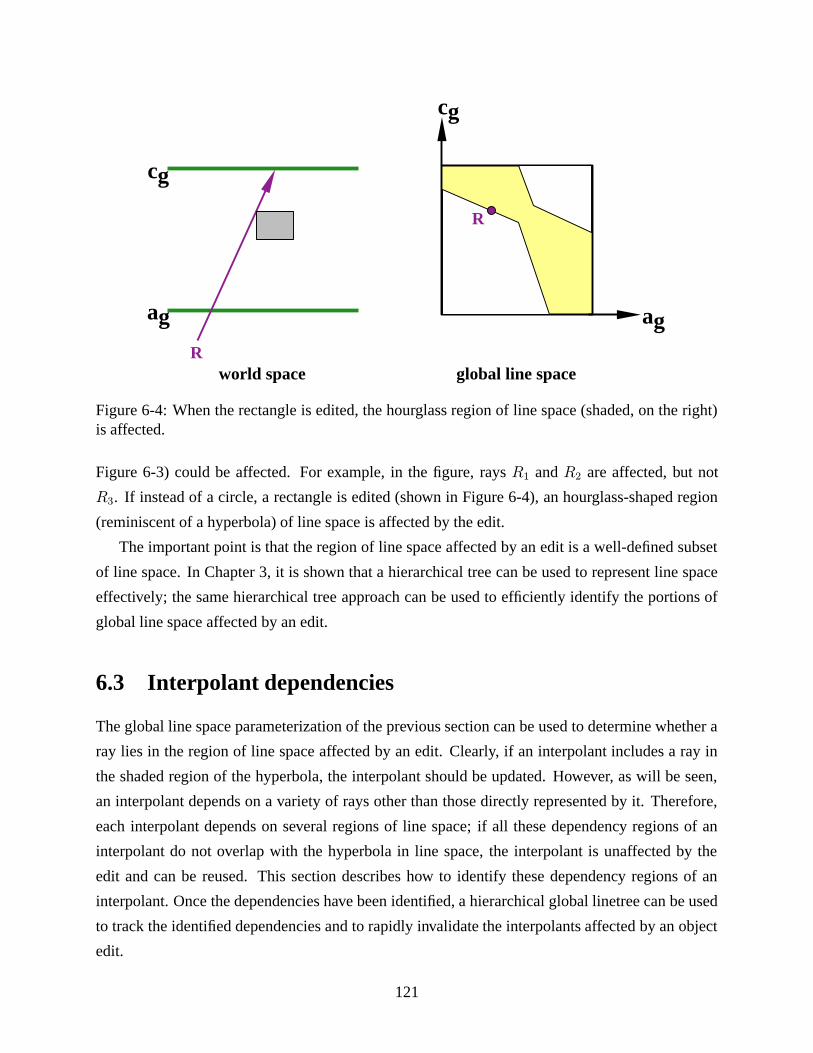
R

ag

cg

ag

cg

R

world space global line space

Figure 6-4: When the rectangle is edited, the hourglass region of line space (shaded, on the right)is affected.

Figure 6-3) could be affected. For example, in the figure, rays R1 and R2 are affected, but not

R3. If instead of a circle, a rectangle is edited (shown in Figure 6-4), an hourglass-shaped region

(reminiscent of a hyperbola) of line space is affected by the edit.

The important point is that the region of line space affected by an edit is a well-defined subset

of line space. In Chapter 3, it is shown that a hierarchical tree can be used to represent line space

effectively; the same hierarchical tree approach can be used to efficiently identify the portions of

global line space affected by an edit.

6.3 Interpolant dependencies

The global line space parameterization of the previous section can be used to determine whether a

ray lies in the region of line space affected by an edit. Clearly, if an interpolant includes a ray in

the shaded region of the hyperbola, the interpolant should be updated. However, as will be seen,

an interpolant depends on a variety of rays other than those directly represented by it. Therefore,

each interpolant depends on several regions of line space; if all these dependency regions of an

interpolant do not overlap with the hyperbola in line space, the interpolant is unaffected by the

edit and can be reused. This section describes how to identify these dependency regions of an

interpolant. Once the dependencies have been identified, a hierarchical global linetree can be used

to track the identified dependencies and to rapidly invalidate the interpolants affected by an object

edit.

121

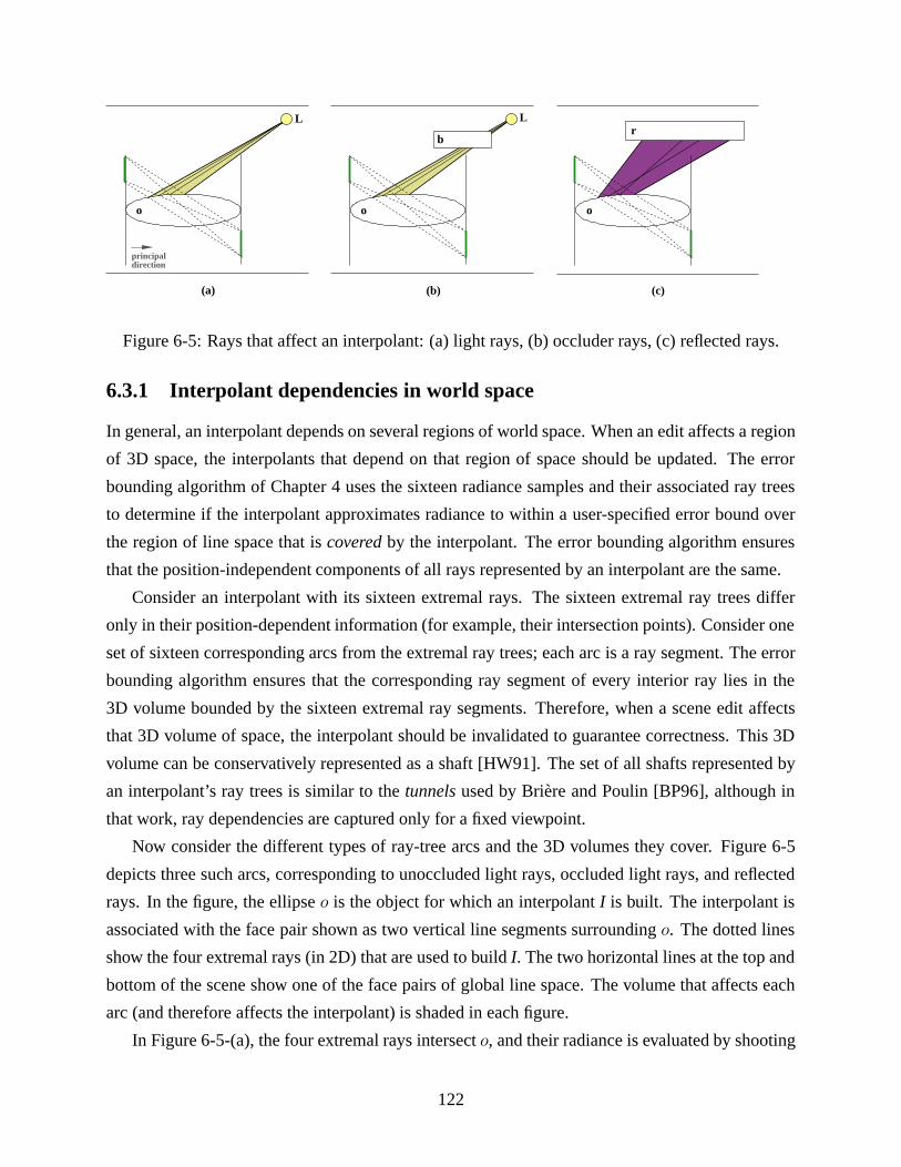
(a)

o

L

principaldirection

(b)

o

L

b

(c)

o

r

Figure 6-5: Rays that affect an interpolant: (a) light rays, (b) occluder rays, (c) reflected rays.

6.3.1 Interpolant dependencies in world space

In general, an interpolant depends on several regions of world space. When an edit affects a region

of 3D space, the interpolants that depend on that region of space should be updated. The error

bounding algorithm of Chapter 4 uses the sixteen radiance samples and their associated ray trees

to determine if the interpolant approximates radiance to within a user-specified error bound over

the region of line space that is coveredby the interpolant. The error bounding algorithm ensures

that the position-independent components of all rays represented by an interpolant are the same.

Consider an interpolant with its sixteen extremal rays. The sixteen extremal ray trees differ

only in their position-dependent information (for example, their intersection points). Consider one

set of sixteen corresponding arcs from the extremal ray trees; each arc is a ray segment. The error

bounding algorithm ensures that the corresponding ray segment of every interior ray lies in the

3D volume bounded by the sixteen extremal ray segments. Therefore, when a scene edit affects

that 3D volume of space, the interpolant should be invalidated to guarantee correctness. This 3D

volume can be conservatively represented as a shaft [HW91]. The set of all shafts represented by

an interpolant’s ray trees is similar to the tunnelsused by Briere and Poulin [BP96], although in

that work, ray dependencies are captured only for a fixed viewpoint.

Now consider the different types of ray-tree arcs and the 3D volumes they cover. Figure 6-5

depicts three such arcs, corresponding to unoccluded light rays, occluded light rays, and reflected

rays. In the figure, the ellipse o is the object for which an interpolant I is built. The interpolant is

associated with the face pair shown as two vertical line segments surrounding o. The dotted lines

show the four extremal rays (in 2D) that are used to build I. The two horizontal lines at the top and

bottom of the scene show one of the face pairs of global line space. The volume that affects each

arc (and therefore affects the interpolant) is shaded in each figure.

In Figure 6-5-(a), the four extremal rays intersect o, and their radiance is evaluated by shooting

122

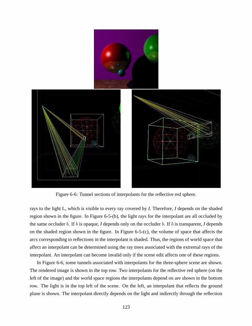
Figure 6-6: Tunnel sections of interpolants for the reflective red sphere.

rays to the light L, which is visible to every ray covered by I. Therefore, I depends on the shaded

region shown in the figure. In Figure 6-5-(b), the light rays for the interpolant are all occluded by

the same occluder b. If b is opaque, I depends only on the occluder b. If b is transparent, I depends

on the shaded region shown in the figure. In Figure 6-5-(c), the volume of space that affects the

arcs corresponding to reflections in the interpolant is shaded. Thus, the regions of world space that

affect an interpolant can be determined using the ray trees associated with the extremal rays of the

interpolant. An interpolant can become invalid only if the scene edit affects one of these regions.

In Figure 6-6, some tunnels associated with interpolants for the three-sphere scene are shown.

The rendered image is shown in the top row. Two interpolants for the reflective red sphere (on the

left of the image) and the world space regions the interpolants depend on are shown in the bottom

row. The light is in the top left of the scene. On the left, an interpolant that reflects the ground

plane is shown. The interpolant directly depends on the light and indirectly through the reflection

123

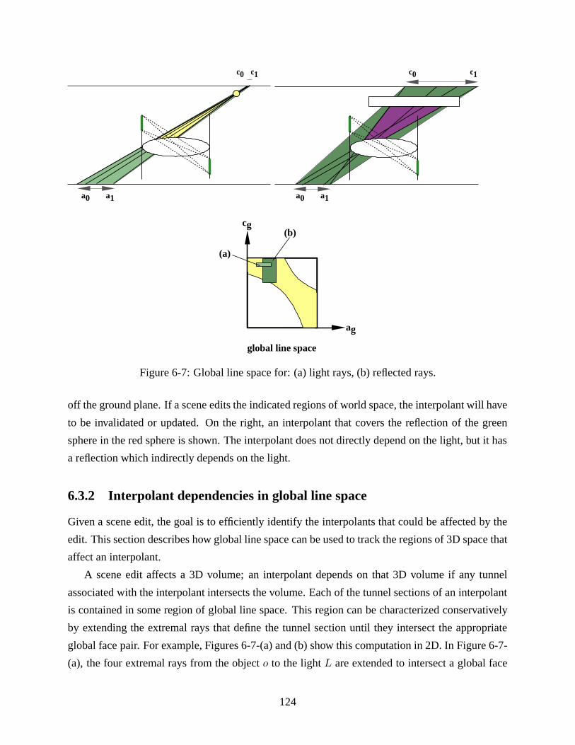
c0 c1

a0 a1a0 a1

c0 c1

ag

cg

global line space

(a)

(b)

Figure 6-7: Global line space for: (a) light rays, (b) reflected rays.

off the ground plane. If a scene edits the indicated regions of world space, the interpolant will have

to be invalidated or updated. On the right, an interpolant that covers the reflection of the green

sphere in the red sphere is shown. The interpolant does not directly depend on the light, but it has

a reflection which indirectly depends on the light.

6.3.2 Interpolant dependencies in global line space

Given a scene edit, the goal is to efficiently identify the interpolants that could be affected by the

edit. This section describes how global line space can be used to track the regions of 3D space that

affect an interpolant.

A scene edit affects a 3D volume; an interpolant depends on that 3D volume if any tunnel

associated with the interpolant intersects the volume. Each of the tunnel sections of an interpolant

is contained in some region of global line space. This region can be characterized conservatively

by extending the extremal rays that define the tunnel section until they intersect the appropriate

global face pair. For example, Figures 6-7-(a) and (b) show this computation in 2D. In Figure 6-7-

(a), the four extremal rays from the object o to the light L are extended to intersect a global face

124

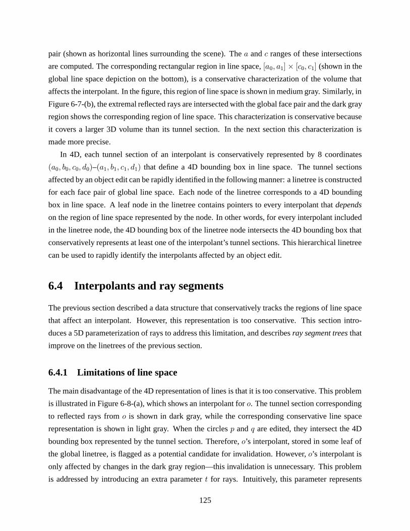
pair (shown as horizontal lines surrounding the scene). The a and c ranges of these intersections

are computed. The corresponding rectangular region in line space, [a0, a1]× [c0, c1] (shown in the

global line space depiction on the bottom), is a conservative characterization of the volume that

affects the interpolant. In the figure, this region of line space is shown in medium gray. Similarly, in

Figure 6-7-(b), the extremal reflected rays are intersected with the global face pair and the dark gray

region shows the corresponding region of line space. This characterization is conservative because

it covers a larger 3D volume than its tunnel section. In the next section this characterization is

made more precise.

In 4D, each tunnel section of an interpolant is conservatively represented by 8 coordinates

(a0, b0, c0, d0)–(a1, b1, c1, d1) that define a 4D bounding box in line space. The tunnel sections

affected by an object edit can be rapidly identified in the following manner: a linetree is constructed

for each face pair of global line space. Each node of the linetree corresponds to a 4D bounding

box in line space. A leaf node in the linetree contains pointers to every interpolant that depends

on the region of line space represented by the node. In other words, for every interpolant included

in the linetree node, the 4D bounding box of the linetree node intersects the 4D bounding box that

conservatively represents at least one of the interpolant’s tunnel sections. This hierarchical linetree

can be used to rapidly identify the interpolants affected by an object edit.

6.4 Interpolants and ray segments

The previous section described a data structure that conservatively tracks the regions of line space

that affect an interpolant. However, this representation is too conservative. This section intro-

duces a 5D parameterization of rays to address this limitation, and describes ray segment treesthat

improve on the linetrees of the previous section.

6.4.1 Limitations of line space

The main disadvantage of the 4D representation of lines is that it is too conservative. This problem

is illustrated in Figure 6-8-(a), which shows an interpolant for o. The tunnel section corresponding

to reflected rays from o is shown in dark gray, while the corresponding conservative line space

representation is shown in light gray. When the circles p and q are edited, they intersect the 4D

bounding box represented by the tunnel section. Therefore, o’s interpolant, stored in some leaf of

the global linetree, is flagged as a potential candidate for invalidation. However, o’s interpolant is

only affected by changes in the dark gray region—this invalidation is unnecessary. This problem

is addressed by introducing an extra parameter t for rays. Intuitively, this parameter represents

125

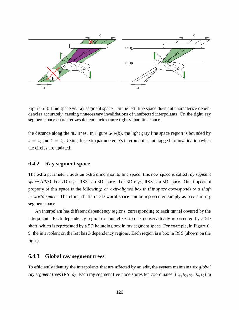
a

c

a

c

t = t1

t = t0o

p

q

Figure 6-8: Line space vs. ray segment space. On the left, line space does not characterize depen-dencies accurately, causing unnecessary invalidations of unaffected interpolants. On the right, raysegment space characterizes dependencies more tightly than line space.

the distance along the 4D lines. In Figure 6-8-(b), the light gray line space region is bounded by

t = t0 and t = t1. Using this extra parameter, o’s interpolant is not flagged for invalidation when

the circles are updated.

6.4.2 Ray segment space

The extra parameter t adds an extra dimension to line space: this new space is called ray segment

space (RSS). For 2D rays, RSS is a 3D space. For 3D rays, RSS is a 5D space. One important

property of this space is the following: an axis-aligned box in this space corresponds to a shaft

in world space. Therefore, shafts in 3D world space can be represented simply as boxes in ray

segment space.

An interpolant has different dependency regions, corresponding to each tunnel covered by the

interpolant. Each dependency region (or tunnel section) is conservatively represented by a 3D

shaft, which is represented by a 5D bounding box in ray segment space. For example, in Figure 6-

9, the interpolant on the left has 3 dependency regions. Each region is a box in RSS (shown on the

right).

6.4.3 Global ray segment trees

To efficiently identify the interpolants that are affected by an edit, the system maintains six global

ray segment trees(RSTs). Each ray segment tree node stores ten coordinates, (a0, b0, c0, d0, t0) to

126

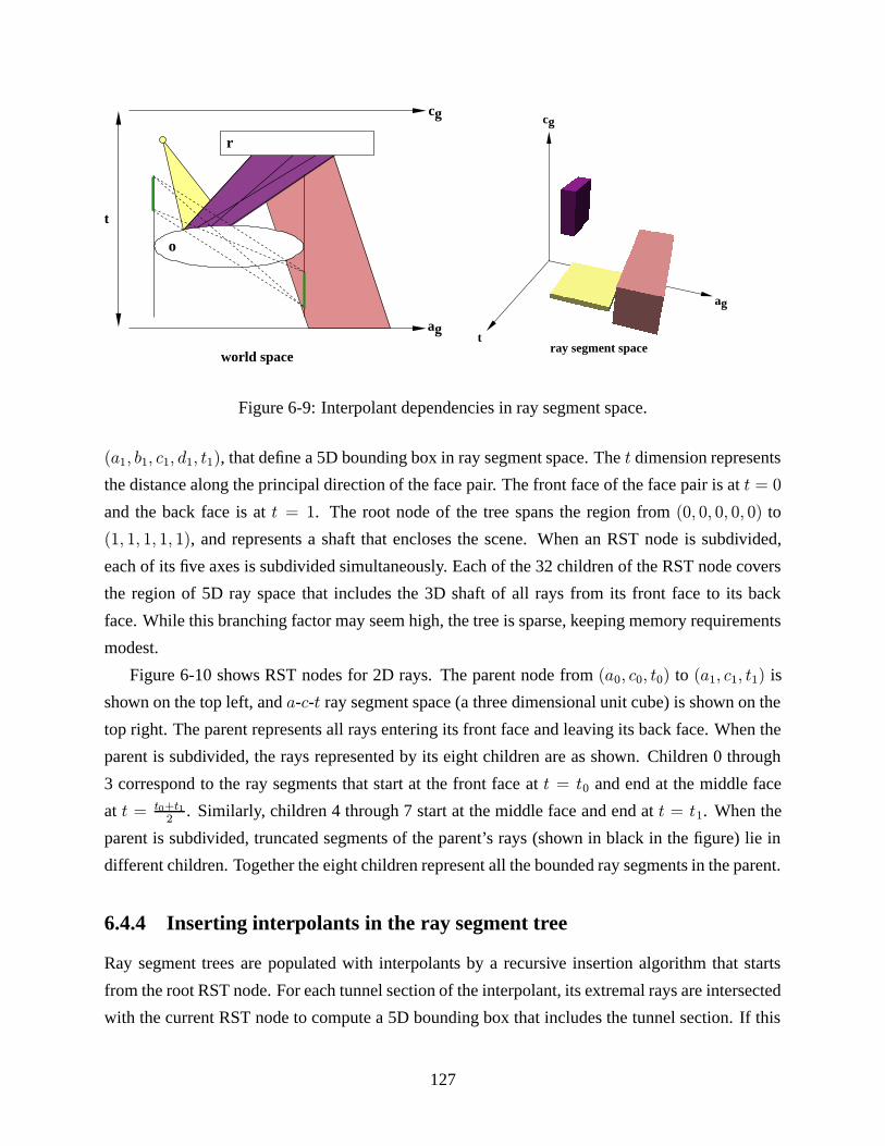
o

r

world space

ag

cg

t

t

ag

cg

ray segment space

Figure 6-9: Interpolant dependencies in ray segment space.

(a1, b1, c1, d1, t1), that define a 5D bounding box in ray segment space. The t dimension represents

the distance along the principal direction of the face pair. The front face of the face pair is at t = 0

and the back face is at t = 1. The root node of the tree spans the region from (0, 0, 0, 0, 0) to

(1, 1, 1, 1, 1), and represents a shaft that encloses the scene. When an RST node is subdivided,

each of its five axes is subdivided simultaneously. Each of the 32 children of the RST node covers

the region of 5D ray space that includes the 3D shaft of all rays from its front face to its back

face. While this branching factor may seem high, the tree is sparse, keeping memory requirements

modest.

Figure 6-10 shows RST nodes for 2D rays. The parent node from (a0, c0, t0) to (a1, c1, t1) is

shown on the top left, and a-c-t ray segment space (a three dimensional unit cube) is shown on the

top right. The parent represents all rays entering its front face and leaving its back face. When the

parent is subdivided, the rays represented by its eight children are as shown. Children 0 through

3 correspond to the ray segments that start at the front face at t = t0 and end at the middle face

at t = t0+t12

. Similarly, children 4 through 7 start at the middle face and end at t = t1. When the

parent is subdivided, truncated segments of the parent’s rays (shown in black in the figure) lie in

different children. Together the eight children represent all the bounded ray segments in the parent.

6.4.4 Inserting interpolants in the ray segment tree

Ray segment trees are populated with interpolants by a recursive insertion algorithm that starts

from the root RST node. For each tunnel section of the interpolant, its extremal rays are intersected

with the current RST node to compute a 5D bounding box that includes the tunnel section. If this

127

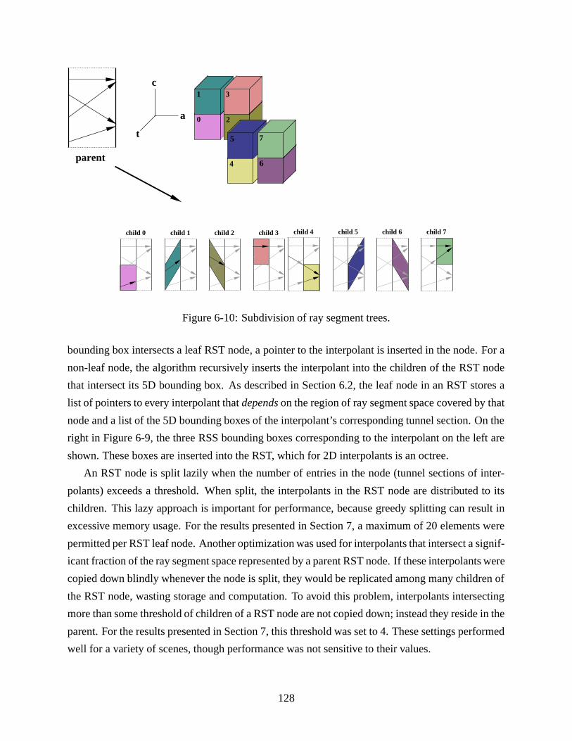
c

t

a

parent

1 3

2

7

4

5

6

0

child 0 child 1 child 2 child 3 child 4 child 5 child 6 child 7

Figure 6-10: Subdivision of ray segment trees.

bounding box intersects a leaf RST node, a pointer to the interpolant is inserted in the node. For a

non-leaf node, the algorithm recursively inserts the interpolant into the children of the RST node

that intersect its 5D bounding box. As described in Section 6.2, the leaf node in an RST stores a

list of pointers to every interpolant that dependson the region of ray segment space covered by that

node and a list of the 5D bounding boxes of the interpolant’s corresponding tunnel section. On the

right in Figure 6-9, the three RSS bounding boxes corresponding to the interpolant on the left are

shown. These boxes are inserted into the RST, which for 2D interpolants is an octree.

An RST node is split lazily when the number of entries in the node (tunnel sections of inter-

polants) exceeds a threshold. When split, the interpolants in the RST node are distributed to its

children. This lazy approach is important for performance, because greedy splitting can result in

excessive memory usage. For the results presented in Section 7, a maximum of 20 elements were

permitted per RST leaf node. Another optimization was used for interpolants that intersect a signif-

icant fraction of the ray segment space represented by a parent RST node. If these interpolants were

copied down blindly whenever the node is split, they would be replicated among many children of

the RST node, wasting storage and computation. To avoid this problem, interpolants intersecting

more than some threshold of children of a RST node are not copied down; instead they reside in the

parent. For the results presented in Section 7, this threshold was set to 4. These settings performed

well for a variety of scenes, though performance was not sensitive to their values.

128

6.5 Using ray segment trees

This section describes how interpolants affected by an object edit are rapidly identified and in-

validated using RSTs. Briere and Poulin [BP96] describe two main categories of object edits:

attribute changes (including changes to an object’s color, specular or diffuse coefficient), and ge-

ometry changes (including insertion or deletion of an object). In their work, attribute and geometry

changes are handled using different mechanisms, since attribute changes can be dealt with rapidly,

while geometry changes require more time. Since the RSTs permit rapid identification of affected

interpolants, the interpolant ray tracer uses the same mechanism to identify affected interpolants

for both types of changes.

6.5.1 Identifying affected interpolants

When an object is edited, 3D shafts [HW91] are used to identify every region of ray segment space,

and therefore every associated interpolant, that is affected by the edit. The identification algorithm

is recursive and starts at each of the six root RST nodes with a world-space region v (the object’s

bounding box) that is affected by an object edit. For each RST node visited recursively, a shaft is

built enclosing the 3D volume between the front and back face of the node. The shaft consists of

six planes: four planes from each edge of the node’s front face to the corresponding edge of its

back face, and two planes that correspond to its front and back faces. If the shaft intersects v, the

children of the RST node are recursively tested for intersection with v. When the shaft of a RST

node does not intersect v, the descendants of that node are not visited. If the RST node is a leaf,

it has a list of pointers to interpolants that depend on the 3D volume represented by the node’s

shaft, and the 5D bounding boxes of their corresponding tunnel sections. A 3D shaft is constructed

for each such tunnel section. If that shaft intersects v, the interpolant is flagged as a candidate for

update. Figure 6-11 shows the interpolants that depend on the reflective mirror at the bottom of the

sculpture in the museum scene shown in Figure 5-8.

One class of interpolant dependencies (depicted in Figure 6-5-(c)), can be identified rapidly

using a different mechanism. While building an interpolant for o, if a light is occluded by an

opaque object b, that tunnel section of the interpolant can be affected when b moves. Therefore, a

separate list of interpolants for occluders is maintained; when b is edited, its list of interpolants is

marked for invalidation.

129

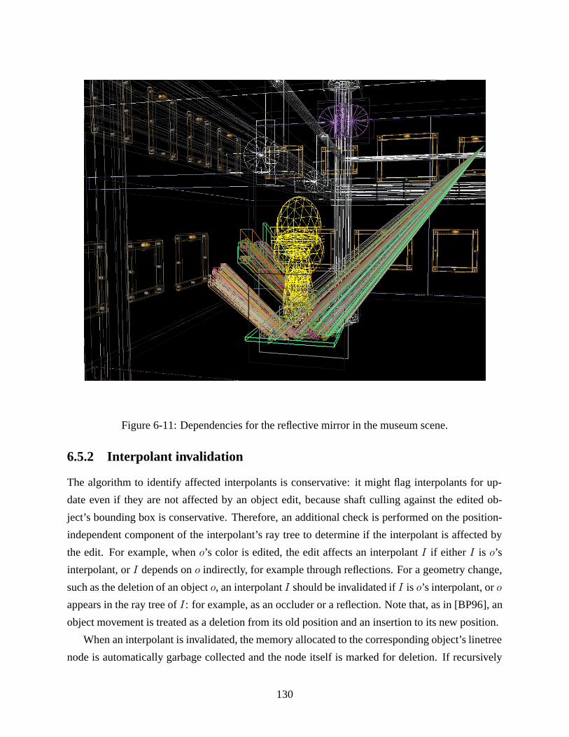
Figure 6-11: Dependencies for the reflective mirror in the museum scene.

6.5.2 Interpolant invalidation

The algorithm to identify affected interpolants is conservative: it might flag interpolants for up-

date even if they are not affected by an object edit, because shaft culling against the edited ob-

ject’s bounding box is conservative. Therefore, an additional check is performed on the position-

independent component of the interpolant’s ray tree to determine if the interpolant is affected by

the edit. For example, when o’s color is edited, the edit affects an interpolant I if either I is o’s

interpolant, or I depends on o indirectly, for example through reflections. For a geometry change,

such as the deletion of an object o, an interpolant I should be invalidated if I is o’s interpolant, or o

appears in the ray tree of I: for example, as an occluder or a reflection. Note that, as in [BP96], an

object movement is treated as a deletion from its old position and an insertion to its new position.

When an interpolant is invalidated, the memory allocated to the corresponding object’s linetree

node is automatically garbage collected and the node itself is marked for deletion. If recursively

130

all that linetree node’s siblings are also invalid, their space is reclaimed, and therefore, the parent

is reclaimed. For example, consider an object o1 that blocks the light to another object o2, causing

o2’s linetrees to be subdivided around o1’s shadow. If o1 is deleted, o2’s interpolants are compacted,

so that no unnecessary subdivision of o2’s linetrees takes place around the shadow that no longer

exists.

To support rapid editing for attribute changes, interpolants could be augmented to include extra

information such as the surface normal and point of intersection for each of the sixteen extremal

rays. Using this extra information, the interpolants could be updated incrementally by computing

the difference in radiance due to the change in o’s material properties [BP96]. However, this

extra position-dependent information increases the memory requirements of interpolants, without

appreciable performance benefits. Therefore, the interpolant ray tracer invalidates interpolants for

both attribute and geometry changes and lazily recomputes them as needed.

6.6 Discussion: pixel-based acceleration for scene editing

A potential optimization for scene editing is to use pixel-based techniques when the viewpoint is

fixed. When extrapolation is not used, the time taken to re-render the scene is dominated by the

time to render failed pixels that cannot be interpolated. In the special case when a user is making

several edits without changing the viewpoint, the cost of rendering failed pixels can be further

reduced by maintaining ray trees for each failed pixel. Because failed pixels account for only

about 8-10% of the pixels in an image, as shown in Chapter 7, the cost of maintaining information

for these pixels is correspondingly lower than in pixel-based scene editing systems.

131

Chapter 7

Performance Results

This chapter evaluates the speed and memory usage of my rendering system by comparing the in-

terpolant ray tracer to the base ray tracer. The results demonstrate that the interpolant ray tracer can

render images substantially faster than the base ray tracer: depending on the level of image quality

desired, rendering is accelerated by a factor of 2.5 to 25. The memory usage of the system is mod-

est and can be bounded using a cache management scheme. This scheme is effective, restricting

total memory usage to 40MB with less than a 1% slowdown. This chapter also presents timing

results for scene editing; it is shown that the ray tracer efficiently updates interpolants affected by

a scene edit.

The rest of this chapter is organized as follows. Section 7.1 presents the base ray tracer and

discusses some performance optimizations for the ray tracer. Section 7.2 describes the test scene

used to evaluate performance. Section 7.3 presents timing results for the interpolant ray tracer,

and Section 7.4 discusses a LRU cache management scheme to bound memory usage. Section 7.5

presents results for scene editing. Section 7.6 discusses how the various extrapolation algorithms

presented in Chapter 5 perform for the museum scene. Section 7.7 discusses how the user can

control performance-quality trade-offs. Section 7.8 discusses issues of interest for multi-processing

the interpolant ray tracer and presents results.

7.1 Base ray tracer

The base ray tracer is a Whitted ray tracer extended to implement the Ward isotropic shading

model [War92] and texturing. The ray tracer supports convex primitives (spheres, cubes, polygons,

cylinders and cones) and the CSG union and intersection of these primitives [Rot82]. The base

ray tracer is used by the interpolant ray tracer for non-interpolated pixels and for constructing

133

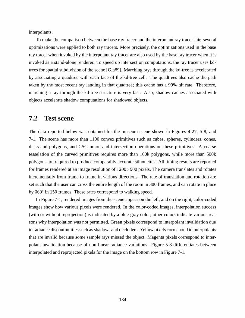
interpolants.

To make the comparison between the base ray tracer and the interpolant ray tracer fair, several

optimizations were applied to both ray tracers. More precisely, the optimizations used in the base

ray tracer when invoked by the interpolant ray tracer are also used by the base ray tracer when it is

invoked as a stand-alone renderer. To speed up intersection computations, the ray tracer uses kd-

trees for spatial subdivision of the scene [Gla89]. Marching rays through the kd-tree is accelerated

by associating a quadtree with each face of the kd-tree cell. The quadtrees also cache the path

taken by the most recent ray landing in that quadtree; this cache has a 99% hit rate. Therefore,

marching a ray through the kd-tree structure is very fast. Also, shadow caches associated with

objects accelerate shadow computations for shadowed objects.

7.2 Test scene

The data reported below was obtained for the museum scene shown in Figures 4-27, 5-8, and

7-1. The scene has more than 1100 convex primitives such as cubes, spheres, cylinders, cones,

disks and polygons, and CSG union and intersection operations on these primitives. A coarse

tesselation of the curved primitives requires more than 100k polygons, while more than 500k

polygons are required to produce comparably accurate silhouettes. All timing results are reported

for frames rendered at an image resolution of 1200×900 pixels. The camera translates and rotates

incrementally from frame to frame in various directions. The rate of translation and rotation are

set such that the user can cross the entire length of the room in 300 frames, and can rotate in place

by 360◦ in 150 frames. These rates correspond to walking speed.

In Figure 7-1, rendered images from the scene appear on the left, and on the right, color-coded

images show how various pixels were rendered. In the color-coded images, interpolation success

(with or without reprojection) is indicated by a blue-gray color; other colors indicate various rea-

sons why interpolation was not permitted. Green pixels correspond to interpolant invalidation due

to radiance discontinuities such as shadows and occluders. Yellow pixels correspond to interpolants

that are invalid because some sample rays missed the object. Magenta pixels correspond to inter-

polant invalidation because of non-linear radiance variations. Figure 5-8 differentiates between

interpolated and reprojected pixels for the image on the bottom row in Figure 7-1.

134

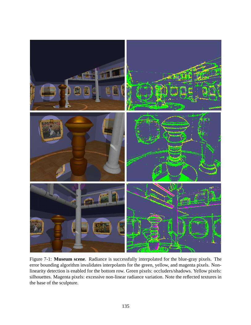
Figure 7-1: Museum scene. Radiance is successfully interpolated for the blue-gray pixels. Theerror bounding algorithm invalidates interpolants for the green, yellow, and magenta pixels. Non-linearity detection is enabled for the bottom row. Green pixels: occluders/shadows. Yellow pixels:silhouettes. Magenta pixels: excessive non-linear radiance variation. Note the reflected textures inthe base of the sculpture.

135

Path Cost for path Average fraction(µs) of pixels covered

Fast path Span fill 1.9 75.2%Reproject 3.9 75.2%Total 5.8 75.2%

Interpolate path Intersect object 24.1 16.88%Find linetree 4.5 16.88%Quad. interpolation 4.2 16.88%Total 32.8 16.88%

Slow path Intersect object 24.1 7.92%Find linetree 4.5 7.92%Test subdivision 11.9 7.49%Build interpolant 645.5 0.43%Shade pixel (base) 160.6 7.92%Weighted total 235.9 7.92%

Interpolant ray tracer 28.5 100.0%Base ray tracer 166.67 100.0%

Table 7.1: Average cost and fraction of pixels for each path over a 60 frame walk-through. Thetotal time for the interpolant ray tracer, shown in the second to last row, is the weighted average ofthe time for each of the three paths. The last row reports the time taken by the base ray tracer.

7.3 Timing results

As described in Section 1.5.1, there are three paths by which a pixel is assigned radiance. These

paths are shown in Figure 1-5 which is reproduced here in Figure 7-2 for ease of reference.

1. Fast path: reprojected data is available and used with the span-filling algorithm.

2. Interpolate path: no reprojected data is available, but a valid interpolant exists. A single

intersection is performed to find the appropriate linetree cell, and radiance is computed by

quadrilinear interpolation.

3. Slow path: no valid interpolant is available, so the cell is subdivided and interpolants are

built if deemed cost-effective. If the built interpolant is invalid, the pixel is rendered by the

base ray tracer.

Table 7.1 shows the costs of each of the three rendering paths. The data for this table was

obtained by using the cycle counter on a single-processor 194 MHz Reality Engine 2, with 512

MB of main memory.

136

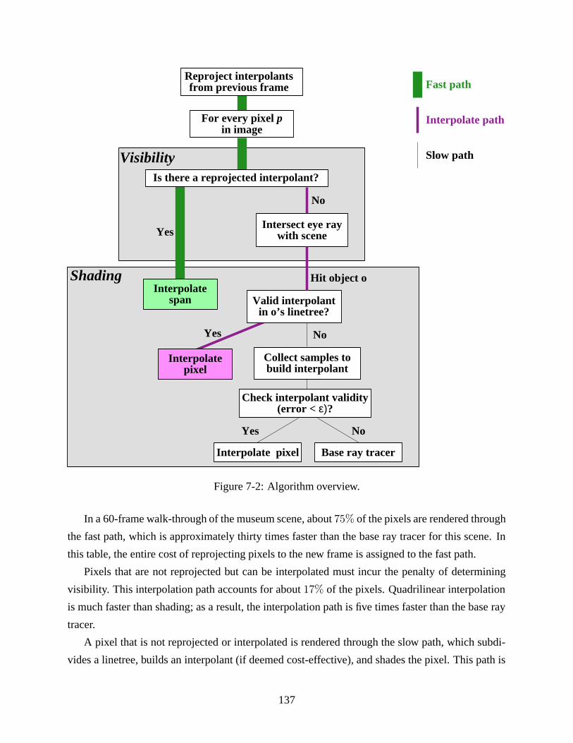
For every pixel pin image

Yes

Visibility

Shading

Reproject interpolantsfrom previous frame

No

Intersect eye raywith scene

Is there a reprojected interpolant?

Hit object o

Yes No

Interpolate pixel

Valid interpolant in o’s linetree?

Yes No

Collect samples tobuild interpolant

Interpolate pixel Base ray tracer

Interpolatespan

Check interpolant validity(error < ε)?

Interpolate path

Fast path

Slow path

Figure 7-2: Algorithm overview.

In a 60-frame walk-through of the museum scene, about 75% of the pixels are rendered through

the fast path, which is approximately thirty times faster than the base ray tracer for this scene. In

this table, the entire cost of reprojecting pixels to the new frame is assigned to the fast path.

Pixels that are not reprojected but can be interpolated must incur the penalty of determining

visibility. This interpolation path accounts for about 17% of the pixels. Quadrilinear interpolation

is much faster than shading; as a result, the interpolation path is five times faster than the base ray

tracer.

A pixel that is not reprojected or interpolated is rendered through the slow path, which subdi-

vides a linetree, builds an interpolant (if deemed cost-effective), and shades the pixel. This path is

137

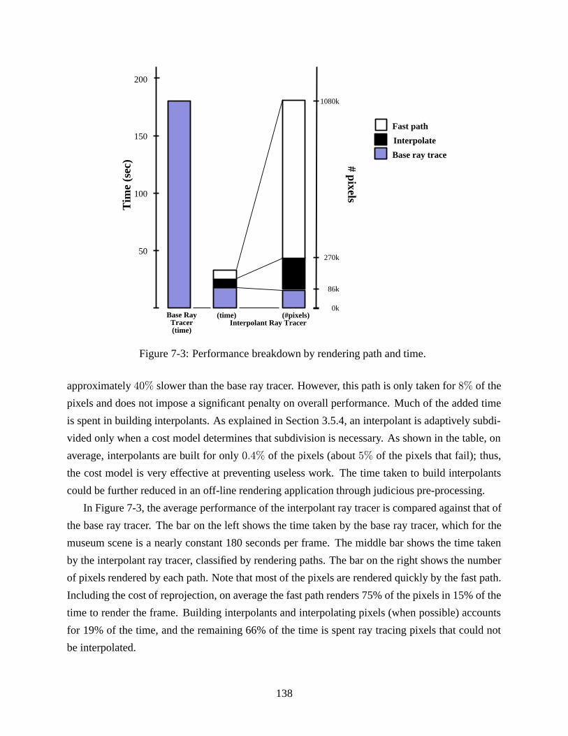
50

100

150

Base RayTracer(time)

Interpolant Ray Tracer

Tim

e (s

ec) # pixels

(#pixels)(time)

Fast path

Interpolate

Base ray trace

200

1080k

270k

86k

0k

Figure 7-3: Performance breakdown by rendering path and time.

approximately 40% slower than the base ray tracer. However, this path is only taken for 8% of the

pixels and does not impose a significant penalty on overall performance. Much of the added time

is spent in building interpolants. As explained in Section 3.5.4, an interpolant is adaptively subdi-

vided only when a cost model determines that subdivision is necessary. As shown in the table, on

average, interpolants are built for only 0.4% of the pixels (about 5% of the pixels that fail); thus,

the cost model is very effective at preventing useless work. The time taken to build interpolants

could be further reduced in an off-line rendering application through judicious pre-processing.

In Figure 7-3, the average performance of the interpolant ray tracer is compared against that of

the base ray tracer. The bar on the left shows the time taken by the base ray tracer, which for the

museum scene is a nearly constant 180 seconds per frame. The middle bar shows the time taken

by the interpolant ray tracer, classified by rendering paths. The bar on the right shows the number

of pixels rendered by each path. Note that most of the pixels are rendered quickly by the fast path.

Including the cost of reprojection, on average the fast path renders 75% of the pixels in 15% of the

time to render the frame. Building interpolants and interpolating pixels (when possible) accounts

for 19% of the time, and the remaining 66% of the time is spent ray tracing pixels that could not

be interpolated.

138

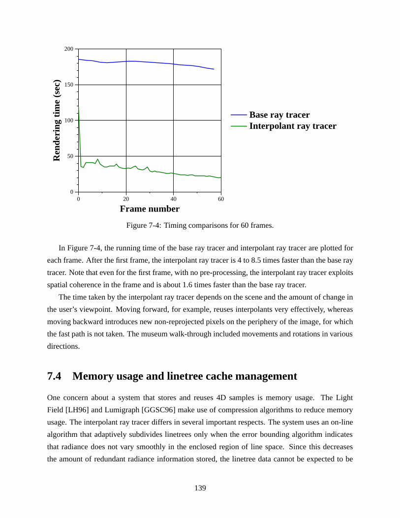
0 20 40 60

Frame number

0

50

100

150

200

Ren

deri

ng t

ime

(sec

)

Base ray tracerInterpolant ray tracer

Figure 7-4: Timing comparisons for 60 frames.

In Figure 7-4, the running time of the base ray tracer and interpolant ray tracer are plotted for

each frame. After the first frame, the interpolant ray tracer is 4 to 8.5 times faster than the base ray

tracer. Note that even for the first frame, with no pre-processing, the interpolant ray tracer exploits

spatial coherence in the frame and is about 1.6 times faster than the base ray tracer.

The time taken by the interpolant ray tracer depends on the scene and the amount of change in

the user’s viewpoint. Moving forward, for example, reuses interpolants very effectively, whereas

moving backward introduces new non-reprojected pixels on the periphery of the image, for which

the fast path is not taken. The museum walk-through included movements and rotations in various

directions.

7.4 Memory usage and linetree cache management

One concern about a system that stores and reuses 4D samples is memory usage. The Light

Field [LH96] and Lumigraph [GGSC96] make use of compression algorithms to reduce memory

usage. The interpolant ray tracer differs in several important respects. The system uses an on-line

algorithm that adaptively subdivides linetrees only when the error bounding algorithm indicates

that radiance does not vary smoothly in the enclosed region of line space. Since this decreases

the amount of redundant radiance information stored, the linetree data cannot be expected to be

139

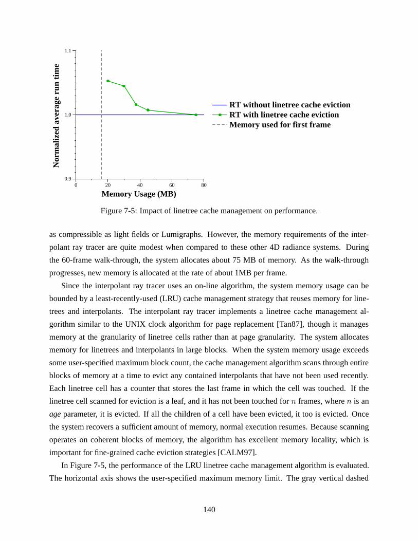
0 20 40 60 80

Memory Usage (MB)

0.9

1.0

1.1N

orm

aliz

ed a

vera

ge r

un t

ime

RT without linetree cache evictionRT with linetree cache evictionMemory used for first frame

Figure 7-5: Impact of linetree cache management on performance.

as compressible as light fields or Lumigraphs. However, the memory requirements of the inter-

polant ray tracer are quite modest when compared to these other 4D radiance systems. During

the 60-frame walk-through, the system allocates about 75 MB of memory. As the walk-through

progresses, new memory is allocated at the rate of about 1MB per frame.

Since the interpolant ray tracer uses an on-line algorithm, the system memory usage can be

bounded by a least-recently-used (LRU) cache management strategy that reuses memory for line-

trees and interpolants. The interpolant ray tracer implements a linetree cache management al-

gorithm similar to the UNIX clock algorithm for page replacement [Tan87], though it manages

memory at the granularity of linetree cells rather than at page granularity. The system allocates

memory for linetrees and interpolants in large blocks. When the system memory usage exceeds

some user-specified maximum block count, the cache management algorithm scans through entire

blocks of memory at a time to evict any contained interpolants that have not been used recently.

Each linetree cell has a counter that stores the last frame in which the cell was touched. If the

linetree cell scanned for eviction is a leaf, and it has not been touched for n frames, where n is an

ageparameter, it is evicted. If all the children of a cell have been evicted, it too is evicted. Once

the system recovers a sufficient amount of memory, normal execution resumes. Because scanning

operates on coherent blocks of memory, the algorithm has excellent memory locality, which is

important for fine-grained cache eviction strategies [CALM97].

In Figure 7-5, the performance of the LRU linetree cache management algorithm is evaluated.

The horizontal axis shows the user-specified maximum memory limit. The gray vertical dashed

140

line shows the memory used when rendering the first frame (17 MB). The vertical axis shows the

average run time of the interpolant ray tracer, normalized with respect to the average run time in

the absence of memory usage restrictions (shown as a flat blue line). The green trace shows that

the cache management algorithm is effective at preventing performance degradation when memory

usage is restricted. Even when memory is restricted to 20 MB, the performance penalty is only

5%; at 45 MB, the penalty is only 0.75%. For long walk-throughs, the benefits of using cache

management far outweigh this small loss in performance. Furthermore, it should be possible to

hide the latency of the cache management algorithm by using idle CPU cycles when the user’s

viewpoint is not changing.

7.5 Scene editing

The part of the system that maintains and uses ray segment trees for scene editing is an optional

module that can be activated selectively. In this section, timing results for scene editing are re-

ported. All timing results are reported for frames rendered on a 250MHz single-processor of an

SGI Infinite Reality. The results consider three edits to the museum scene, as shown in Figure 7-6:

the top of the sculpture is deleted (Edit-(a)), the bottom of the sculpture is deleted (Edit-(b)), a

green cube is moved in on the right (Edit-(c)). When the user changes the viewpoint, new inter-

polants are built as required.

Figure 7-6 shows the impact of these edits on interpolants. On the left, rendered images are

shown, and on the right are color-coded images showing the regions of interpolation failure and

success. As before, green, yellow pixels are not interpolated due to radiance discontinuities such

as shadow edges and object silhouettes. Pixels that are successfully interpolated are shown in dark

blue. The red pixels show the interpolants that are invalidated and rebuilt when the scene is edited.

For example, after Edit-(a), the top of the sculpture and the shadow behind it are updated; the

new interpolants lazily built to cover those pixels are shown in red. After Edit-(b), the interpolants

associated with the bottom of the sculpture and its reflection in the mirror are found and invalidated.

Table 7.2 presents performance results for time and memory usage for scene edits. A change

to the viewpoint is considered a scene edit, except that no interpolants are invalidated by the view-

point change. This is because interpolants do not depend on the current viewpoint. For each of the

edits, traversing the RSTs and invalidating the corresponding linetrees is fast: it takes about a tenth

of a second. This is considerably faster than the invalidation process in pixel-based ray tracers

supporting scene editing [BP96]. Depending on the type of edit, and its impact on interpolants,

updating interpolants lazily while re-rendering a frame takes 4.5 to 14 seconds using the extrapo-

141

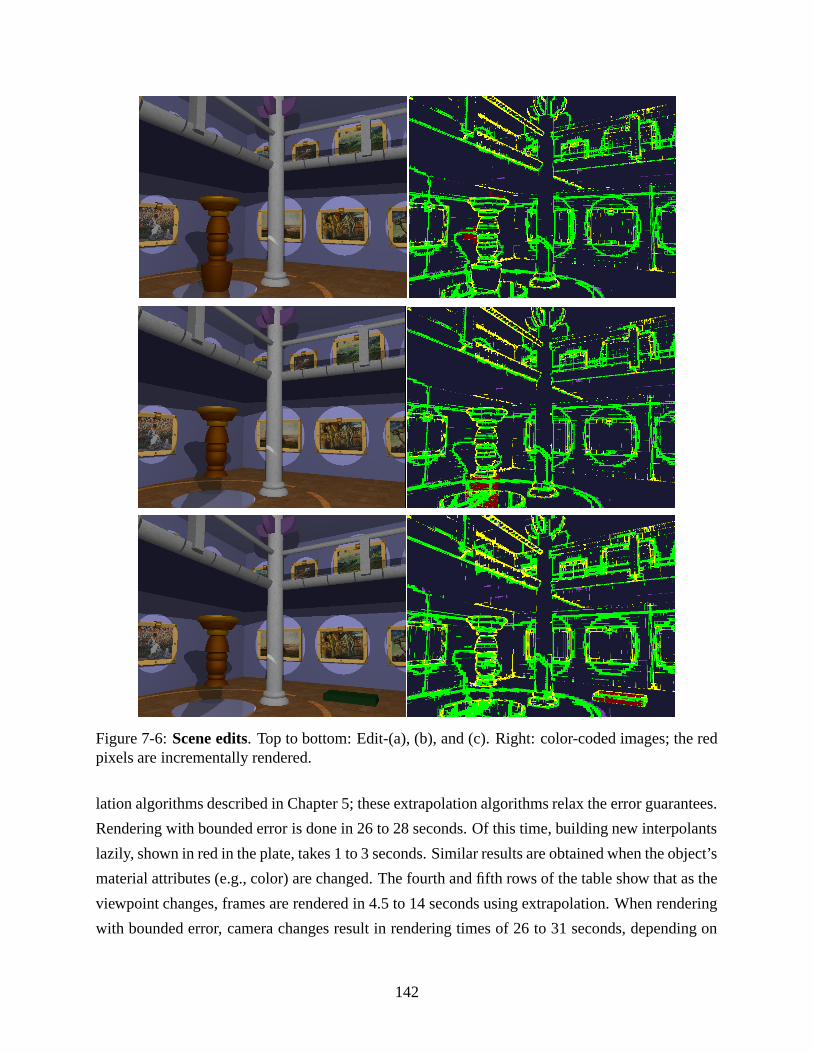
Figure 7-6: Scene edits. Top to bottom: Edit-(a), (b), and (c). Right: color-coded images; the redpixels are incrementally rendered.

lation algorithms described in Chapter 5; these extrapolation algorithms relax the error guarantees.

Rendering with bounded error is done in 26 to 28 seconds. Of this time, building new interpolants

lazily, shown in red in the plate, takes 1 to 3 seconds. Similar results are obtained when the object’s

material attributes (e.g., color) are changed. The fourth and fifth rows of the table show that as the

viewpoint changes, frames are rendered in 4.5 to 14 seconds using extrapolation. When rendering

with bounded error, camera changes result in rendering times of 26 to 31 seconds, depending on

142

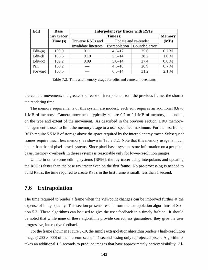
Edit Base Interpolant ray tracer with RSTsray tracer Time (s) MemoryTime (s) Traverse RSTs and Update and re-render (MB)

invalidate linetrees Extrapolation Bounded errorEdit-(a) 109.0 0.11 4.5–12 25.6 0.7 MEdit-(b) 108.6 0.10 5.5–14 28.2 1.0 MEdit-(c) 109.2 0.09 5.0–14 27.4 0.6 MPan 108.2 — 4.5–10 26.9 0.7 MForward 108.5 — 6.5–14 31.2 2.1 M

Table 7.2: Time and memory usage for edits and camera movements.

the camera movement; the greater the reuse of interpolants from the previous frame, the shorter

the rendering time.

The memory requirements of this system are modest: each edit requires an additional 0.6 to

1 MB of memory. Camera movements typically require 0.7 to 2.1 MB of memory, depending

on the type and extent of the movement. As described in the previous section, LRU memory-

management is used to limit the memory usage to a user-specified maximum. For the first frame,

RSTs require 5.5 MB of storage above the space required by the interpolant ray tracer. Subsequent

frames require much less memory, as shown in Table 7.2. Note that this memory usage is much

better than that of pixel-based systems. Since pixel-based systems store information on a per-pixel

basis, memory overheads in these systems is reasonable only for lower-resolution images.

Unlike in other scene editing systems [BP96], the ray tracer using interpolants and updating

the RST is faster than the base ray tracer even on the first frame. No pre-processing is needed to

build RSTs; the time required to create RSTs in the first frame is small: less than 1 second.

7.6 Extrapolation

The time required to render a frame when the viewpoint changes can be improved further at the

expense of image quality. This section presents results from the extrapolation algorithms of Sec-

tion 5.3. These algorithms can be used to give the user feedback in a timely fashion. It should

be noted that while none of these algorithms provide correctness guarantees; they give the user

progressive, interactive feedback.

For the frame shown in Figure 5-10, the simple extrapolation algorithm renders a high-resolution

image (1200× 900) of the museum scene in 4 seconds using only reprojected pixels. Algorithm 3

takes an additional 1.5 seconds to produce images that have approximately correct visibility. Al-

143

gorithm 4 produces an image that is visually almost indistinguishable from the “correct” image,

shown in Figure 5-11, in a total of 10 seconds.

Note that the extrapolation algorithm that guarantees correct visibility determination at each

pixel of the image, Algorithm 2, takes a total of 9 seconds. In general, images produced by Al-

gorithm 2 and Algorithm 3 are visually similar, though Algorithm 2 guarantees correct visibility

determination at an increased cost, while Algorithm 3 achieves good performance with occasional

errors due to incorrect visibility determination.

The final pass fills the failed pixels (the slow path) in about 18 more seconds, resulting in the

image that the interpolant ray tracer produces. The advantage of this approach is that the user gets

feedback rapidly, in 4 to 9 seconds, which is about 10 times faster than the base ray tracer for this

image, with image quality comparable to the base ray tracer.

Although the results in this chapter are reported for images of 1200 × 900 pixels to allow a

consistent basis for comparison, it is interesting to consider the performance of the renderer at

lower resolution. Not surprisingly, the images at NTSC resolution (640 × 480 pixels) take less

time to render. At this resolution, the simple extrapolation algorithm produces an image of the

museum scene in 1.6 seconds. Algorithm 3 produces images in an extra 0.9 seconds; Algorithm 4

produces images in an additional 2.0 seconds. The failed pixels are then rendered in another 5-6

seconds. Thus, the user receives feedback quickly enough for practical interactive use.

Depending on the coherence in the scene, these progressive techniques provide rapid feedback

(10× to 15× speedup over the base ray tracer) with good image quality.

7.7 Performance vs. image quality

The user-supplied error parameter ε allows graceful control of the computation expended per

frame; a larger permitted error permits extended re-use of interpolants, and less computation ex-

pended per frame. Of course, this performance is achieved with lower image quality. A small

permitted error results in longer inter-frame delays but produces higher image quality.

The interpolant ray tracer supports a number of different ways to trade performance for ren-

dering quality. A comparison of these techniques is shown in Figure 7-7. The vertical axis of

this plot shows the time required to render the museum scene. Note that the base ray tracer takes

about 109 seconds to render this scene. Three different traces, marked by squares, diamonds, and

circles, show the time required to accomplish three different rendering tasks with varying bounds

on rendering error. For the trace marked by squares, the ray tracer is rendering the scene from a

camera position forward from its previous position. For the trace marked by diamonds, the camera

144

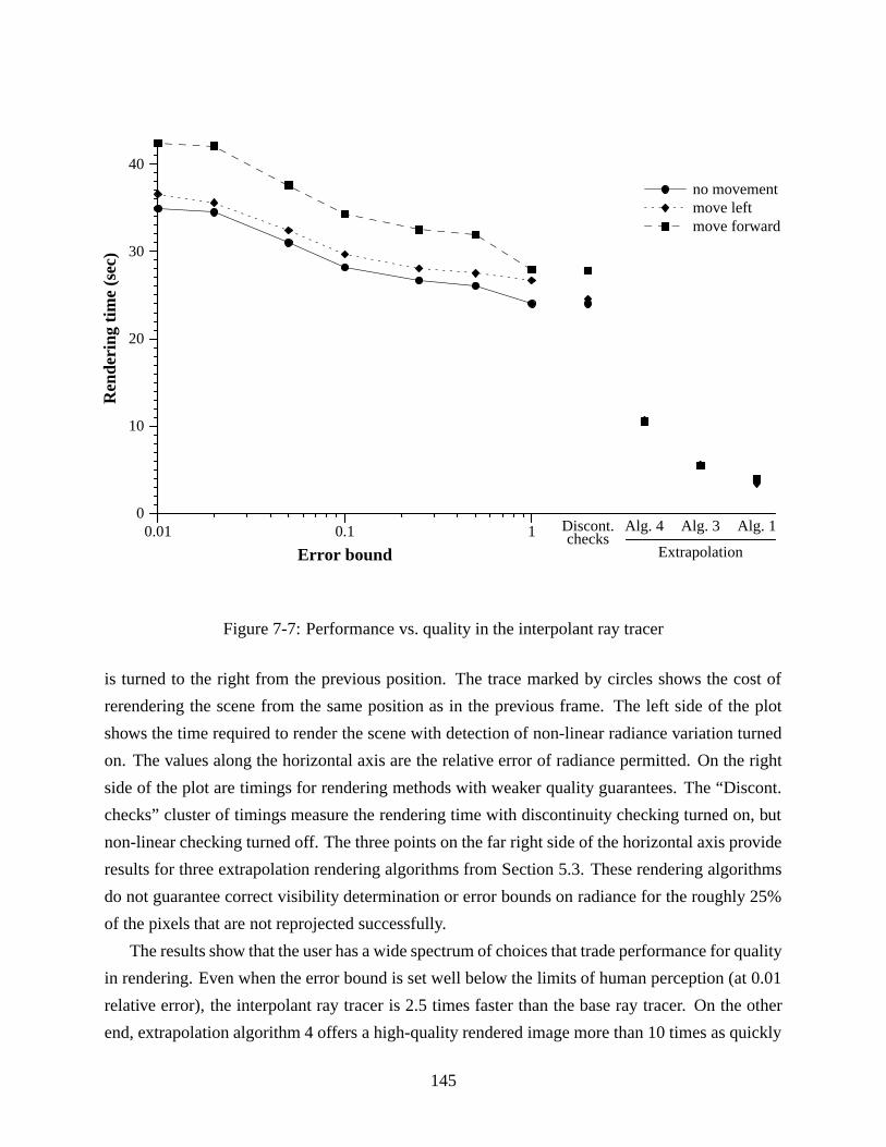
0.01 0.1 1

Error bound

0

10

20

30

40

Ren

deri

ng t

ime

(sec

)

no movementmove leftmove forward

Extrapolation

Discont.checks

Alg. 4 Alg. 3 Alg. 1

Figure 7-7: Performance vs. quality in the interpolant ray tracer

is turned to the right from the previous position. The trace marked by circles shows the cost of

rerendering the scene from the same position as in the previous frame. The left side of the plot

shows the time required to render the scene with detection of non-linear radiance variation turned

on. The values along the horizontal axis are the relative error of radiance permitted. On the right

side of the plot are timings for rendering methods with weaker quality guarantees. The “Discont.

checks” cluster of timings measure the rendering time with discontinuity checking turned on, but

non-linear checking turned off. The three points on the far right side of the horizontal axis provide

results for three extrapolation rendering algorithms from Section 5.3. These rendering algorithms

do not guarantee correct visibility determination or error bounds on radiance for the roughly 25%

of the pixels that are not reprojected successfully.

The results show that the user has a wide spectrum of choices that trade performance for quality

in rendering. Even when the error bound is set well below the limits of human perception (at 0.01

relative error), the interpolant ray tracer is 2.5 times faster than the base ray tracer. On the other

end, extrapolation algorithm 4 offers a high-quality rendered image more than 10 times as quickly

145

as the base ray tracer; the other extrapolation algorithms offer speedup of up to 25×, though with

more noticeable rendering artifacts.

Not shown in the figure is the time required to render the first frame. The rendering time for

the first frame is faster in the interpolant ray tracer than in the base ray tracer for all the error

settings except those in which ε ≤ 0.05. Even at the setting of ε = 0.01, the interpolant ray

tracer exhibits only a 16% slowdown rendering the first frame when compared to the base ray

tracer. This slowdown occurs because the first frame requires the building of more interpolants

than subsequent frames do. The fastest technique for rendering the first frame is to check only for

discontinuity errors; the interpolant ray tracer is 1.6 times faster than the base ray tracer with this

technique. Note that the extrapolation algorithms cannot be used to render the first frame because

they rely on reprojected data from previous frames.

7.8 Multi-processing

Another technique for improving interactive performance is to use multiple processors to render

the image. It should be noted that this technique also improves the performance of the base ray

tracer. The interpolant ray tracer has been extended to run on a multiprocessor machine.

Two major issues should be considered when parallelizing a ray tracer: load balancing and

memory contention. To achieve balanced loads when rendering a frame, the interpolant ray tracer

divides an image into square chunks that are queued to the processors available. A work queue

algorithm [BL94] is used to obtain balanced work-loads on each processor.

Several steps are taken to decrease memory contention between competing processors. The

only data structure shared by the processors is the linetree. For example, each processor maintains

its own common-ray hash tables to cache radiance samples, and performs all memory allocation

using its own memory arenas. For the common-ray hash tables, it is less expensive to occasionally

recompute radiance for some rays than to synchronize on every hash table access.

Because the linetree data structures are shared across all the processors, locks are placed in

linetree nodes to prevent race conditions. However, the data structure is designed in such a way that

interpolant lookups do not require any locking of linetree nodes. Locking is only required when

inserting an interpolant into the linetree and when subdividing a linetree node. These optimizations

greatly reduce the locking overhead, since multiple processors simultaneously read from the same

linetree. Processors only block each other when updating the same linetree.

The shaft-culling phase of reprojection has not been parallelized, although it could be. The

speedup for parallelizing shaft-culling should be nearly linear because workload balancing is

146

straight-forward and shaft culling is a computationally intensive (rather than memory-intensive)

operation.

On a four-processor Reality Engine, rendering speedup is about 2.8× to 3.5× for the interpolant

ray tracer. Speedup for the base ray tracer is slightly better, about 3.8×. This effect is to be

expected because the interpolant ray tracer is a memory-intensive computation, and there is some

memory contention between the processors. In addition, certain parts of the interpolant ray tracer

are not parallelized in the current implementation.

147

Chapter 8

Conclusions and Future Work

This thesis presents the concept of radiance interpolants, which are used to approximate radiance

while bounding approximation error. Interpolants allow ray tracing to be accelerated by exploiting

object-space, ray-space, image-space and temporal coherence. The interpolant ray tracer described

in this thesis uses radiance interpolants to accelerate both shading and visibility determination. The

ray tracer also uses interpolants to support incremental ray tracing while permitting the user to edit

the scene and the current viewpoint.

8.1 Contributions

Several new concepts and algorithms are introduced in this thesis:

• Radiance interpolants:This thesis demonstrates how radiance interpolants can be used to

effectively capture the coherence in the radiance function. The thesis describes the inter-

polant construction mechanism that is used to sample the radiance function sparsely and

reconstruct radiance. Hierarchical data structures over line space, called linetrees, are used

to store radiance samples and facilitate efficient reconstruction of the radiance function.

• Error bounds and error-driven sampling:This thesis introduces novel geometric and ana-

lytical techniques to bound interpolation error. An error bounding algorithm is used to guide

adaptive subdivision; where the error bounding algorithm indicates possible interpolation

error, radiance is sampled more densely. Interpolation error arises both from discontinuities

and non-linearities in the radiance function. The error bounding algorithm automatically

and conservatively prevents interpolation in both these cases. Novel geometric techniques

detect discontinuities. The thesis also describes how linear interval arithmetic can be ap-

plied to bounding non-linear radiance variations. To the best of my knowledge this is the

149

first accelerated ray tracer that bounds interpolation error conservatively. The error bound-

ing algorithm is efficient and provides an accurate estimate of error; these properties are

both important for its use in accelerating ray tracing. The thesis also demonstrates that error

bounds can be used by the user to trade performance for quality. Even when the permitted

error is very low, the interpolant ray tracer still accelerates rendering substantially.

• Reprojection for visibility acceleration:Determination of the visible surface for each pixel

is accelerated by a novel reprojection algorithm that exploits temporal frame-to-frame co-

herence in the user’s viewpoint, but guarantees correctness.

• Interpolants for scene editing:This thesis presents the first ray tracer that supports incre-

mental ray tracing with scene editing while permitting changes in the user’s viewpoint.

Interpolants are shown to provide an efficient mechanism for incremental update of radiance

when the scene is edited. The concept of ray segment space is introduced for scene editing;

this five-dimensional space is useful because a bounding box in this space is a shaft in 3D

space. This concept is used to identify the regions of world space that affect an interpolant.

An auxiliary data structure, the ray segment tree, is built over ray segment space; when the

scene is edited, ray segment trees are rapidly traversed to identify affected interpolants.

The performance results demonstrate that the interpolant ray tracer offers significant speedup.

It successfully exploits coherence in radiance to accelerate ray tracing by a factor of 4× to 15×.

For the museum scene, the interpolant ray tracer accelerates 92% of the pixels, and only 8% of the

pixels are rendered using the base ray tracer. For improved interactive feedback, the ray tracer also

supports extrapolation algorithms that allow rendering of the scene without error guarantees in a

few seconds. These extrapolation algorithms can be applied progressively in sequence, converging

on an image with bounded error. For scene editing, the ray segment tree data structure allows

identification of affected interpolants very rapidly; invalidation of these interpolants takes about

0.1 seconds in the museum scene. The additional overhead incurred when inserting information

into the ray segment tree is less than 2%. Additionally, the thesis describes how a simple cache

management algorithm can efficiently bound memory usage, keeping the memory requirements of

the interpolant ray tracer modest.

8.2 Future work and extensions

The techniques presented in this thesis should be applicable to a variety of applications; some

of these applications are discussed in this section. This section also discusses future avenues of

150

research that must be explored to support the extensions described in Section 4.5.

8.2.1 Animations and modeling

Animators should substantially benefit from the use of the interpolant ray tracer. An animator

typically works in a model-render-model cycle in which he models the scene, previews his results

by rendering the animation, and then uses these previewed animations to refine his model. Finally,

once he has finalized his animation, he uses the ray tracer to produce high-quality images for final

viewing. The interpolant ray tracer described in this thesis could be used to accelerate rendering

and to improve the quality of the interactions that the animator has with the system in each of these

phases of the creation of an animation.

There are several ways in which the interpolant ray tracer could be useful for this application.

As the animator changes the scene, the interpolant ray tracer could incrementally render the scene

to provide rapid feedback using the techniques developed in this thesis for scene editing. Once

the animator is done modeling, the interpolant ray tracer could be used to rapidly compute images

for previewing. The animator could use error bounds to trade performance for quality while pre-

viewing images. Finally, when the animator is ready to produce the high-quality animation, the

techniques described in this thesis could be used to accelerate the rendering of the animation.

The following extensions to the interpolant ray tracer could further enhance the utility of the

interpolant ray tracer for this application.

Persistence. A persistent store interface could be used to store interpolants as they are built for

previews. These stored interpolants then could be reused from session to session as the animator

refines the scene. As the animator edits the scene, the appropriate interpolants could be invalidated

or reused appropriately. Once the animator is done modeling the scene and wants to create the

final animation, he can invoke the interpolant ray tracer to render the animation with high quality

(i.e., small ε). The interpolants stored in persistent storage could be reused to produce the final an-

imation, provided they satisfy the error bound. Thus, the system could build and reuse interpolants

from modeling sessions to final animations incrementally. There are several interesting systems

issues that should be addressed to achieve this goal: for example, how to represent radiance in per-

sistent storage and how to compress large radiance data sets effectively. Funkhouser et al. [FST92]

address storage issues for large radiosity data sets; some of their techniques should be applicable

to this problem. IBR systems [GGSC96, LH96] present techniques to compress 4D radiance in-

formation; these techniques should be applicable to the compression of radiance interpolants as

well. However, since linetrees are not uniformly subdivided arrays, and interpolants already cap-

151

ture coherence in radiance, compression rates cannot be expected to be as high as in these previous

systems.

Representing time explicitly. Animations typically have pre-defined trajectories for objects and

the viewpoint. A useful extension would be to explicitly sample the temporal dimension when

building interpolants. The domain over which samples are collected is then a five dimensional

space, a temporal-line space. Glassner [Gla88] considers using a four dimensional spatio-temporal

space to accelerate animations. The 5D temporal-line space described here is similar in spirit to

Glassner’s spatio-temporal space, although in this case, the interpolants would store time-varying

radiance information. This approach opens an interesting avenue of research: translating error

guarantees in 4D line space to meaningful error guarantees in 5D temporal-line space. It will be

necessary to refine the invariant maintained by the error bounding algorithm, developing a notion

of temporal error.

8.2.2 Architectural walk-throughs

Ray tracing is often used to produce high-quality imagery in large off-line animations for archi-

tectural walk-throughs and other visualizations. The techniques introduced in this thesis should be

useful in accelerating both these pre-programmed animations and interactive walk-throughs. As

described above, the interpolant ray tracer can be used directly for a pre-programmed animation

where the user completely specifies a camera path. An interesting extension would be to support

accelerated rendering when the user does not specify the entire camera position. Note that if the

user provides absolutely no viewing information to the interpolant ray tracer, the ray tracer would

start sampling the radiance function from all possible viewpoints. This could be prohibitively

expensive. However, sampling could be limited usefully if the user provided an approximate de-

scription of the viewing trajectory; for example, the viewpoint could be restricted to a set of rooms

in a building, or the user could provide a notion of the important features in the building for which

interpolants could be built. This information would be used by the ray tracer to guide where sam-

ples are collected in the space of rays. This approach suggests several interesting areas of research.

8.2.3 Intelligent, adaptive sampling

When rendering high-resolution images, ray tracers typically must resolve a tension between sub-

sampling the image to achieve good rendering performance, and super-sampling the image to

achieve good image quality. While a ray tracer can achieve good performance by sampling an

image sparsely, image quality may suffer because the ray tracer may miss small features, high-

152

lights, small reflections and shadows. These small features are important to the human perceptual

system, particularly when animations are rendered; missing small features in some frames while

capturing them in others results in disturbing speckling artifacts.

Existing algorithms that use adaptive sampling typically require hand tuning to ensure that

good quality results are achieved with good performance. Also, these algorithms typically can-

not accommodate varying sampling rates across an image: coarse sub-sampling is desired in the

parts of the image where radiance varies smoothly, and super-sampling is needed where radiance

changes rapidly. It is important to have quality assurances that are robust, automatically enforced

without hand-tuning, and that permit sparse sampling where possible for good performance.

Independent of the interpolant mechanisms, the error bounding techniques described in this

thesis should be applicable to this problem of adaptive sampling. Because the error bounding algo-

rithm is able to characterize how the radiance function varies over ray space, this characterization

could be used to guide intelligent sampling of images that provide good performance. The error

bounding algorithm would allow computational resources to be focused automatically on the parts

of the image that must be super-sampled at greater resolution, while identifying the parts of the

image that can be sampled sparsely.

8.2.4 Perception-based error metrics

One area of research that is gaining prominence in computer graphics is the use of perception-based

error metrics in rendering [FPSG96, FPSG97, PFFG98, BM98]. The error bounding algorithm

presented in this thesis is used to bound either actual or relative error in radiance; however, since

discontinuities are important to the visual system, they are treated as a special case. An interesting

area of future research would be to generalize the error techniques presented in this thesis to capture

other perceptually-important aspects of radiance variation. These perceptual techniques would

complement the existing error bounding algorithm.

8.2.5 Generalized shading model, geometry and scene complexity

Section 4.5 describes several possible extensions to the system that extend its shading model and

permit greater geometric, lighting, and scene complexity.

Non-convex and parametric surfaces. One limitation of the interpolant ray tracer is that it can

only guarantee error bounds for convex primitives. Interpolants are not built for non-convex prim-

itives; therefore, rendering of these primitives is not accelerated. The interpolation mechanism

153

remains the same for these primitives; the main research problem to be solved is extension of the

error bounding algorithm to support these primitives.

Section 4.3 briefly sketches how interval arithmetic might be generalized to support non-convex

objects described by parametric patches. The linear interval approach is easily applied to any

surface defined by an implicit equation. To apply it to parametric surfaces requires the ability to

solve for the surface patch parameters s and t in order to obtain accurate bounds on the surface

normal. This can be accomplished using interval-based root finding, which generalizes to linear

intervals [Han75].

Non-convex objects can be supported in a number of ways. One simple, conservative approach

is to bound a non-convex object o on the inside and outside by convex objects. For complex non-

convex objects, the object o can be broken into smaller pieces to allow these bounding convex

objects to closely approximate the surface of o. For those parts of the error bounding computation

that depend on convexity, such as the tests for shadow edge discontinuities, one or both of these

convex objects can be used in place of o to ensure that error is bounded conservatively.

Textures. It would be useful to expand the support for textures in the interpolant ray tracer to

include more general texturing techniques, such as bump maps and displacement maps. Bounds

on perturbed surface positions and normals can be extracted for each interpolant from the region

of the map corresponding to the object surface area covered by the interpolant. These bounds can

then be applied in a straightforward manner to the linear interval analysis equations in Section 4.3.

Other extended texturing techniques of interest include maps for specular and reflective surface

coefficients. A similar bounding technique should be applicable for these maps as well.

Diffuse global illumination. Extending the ray tracer to compute diffuse inter-reflections and

generalized BRDFs would be useful. The research question that must be addressed for this to be

feasible is how to manage the increased complexity due to extra links to other sources of energy.

The invariant defined in Section 4.1.1 could be relaxed to permit interpolation across small

discontinuities; understanding the implications of relaxing this invariant is an important research

area. Importance-driven techniques [SAS92] could be used to track the important sources of light

energy for each interpolant. Sources of energy that contribute light energy below the error threshold

would be ignored. The error bounding algorithm would use this relaxed invariant of error, so

a detected discontinuity would invalidate an interpolant only if the resulting interpolation error

exceeds the user-specified bound. While the error guarantees will continue to be satisfied, the

implication of this relaxed error invariant on perceived error deserves detailed study.

154

Clustered lights, area lights, large number of lights. Support for more general light sources,

such as area light sources, clustered lights, and increased lighting complexity would be useful. As

described above, in this case the invariant maintained by the error bounding algorithm could be re-

laxed to permit interpolation across discontinuities that are not important. While some researchers

are studying the problems associated with clustered lights, area lights and their implications on illu-

mination [PPD98, War91, SS98, WH98], computing error bounds with these forms of illumination

is an open area of research.

155

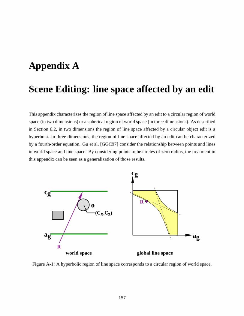
Appendix A

Scene Editing: line space affected by an edit

This appendix characterizes the region of line space affected by an edit to a circular region of world

space (in two dimensions) or a spherical region of world space (in three dimensions). As described

in Section 6.2, in two dimensions the region of line space affected by a circular object edit is a

hyperbola. In three dimensions, the region of line space affected by an edit can be characterized

by a fourth-order equation. Gu et al. [GGC97] consider the relationship between points and lines

in world space and line space. By considering points to be circles of zero radius, the treatment in

this appendix can be seen as a generalization of those results.

R

ag

cg

R

world space global line space

ag

cg

o(Cx,Cz)

Figure A-1: A hyperbolic region of line space corresponds to a circular region of world space.

157

A.1 Edits in two dimensions

Consider a scene and its four global segment pairs. In Figure A-1, one of the four segment pairs

(the pair of thick horizontal lines), with +z as principal direction, is shown on the left. When a

circular object o is edited, every ray that passes through o is affected by the edit.

Claim: The region of line space (shown as a square on the right of the figure) affected by edits to

o is the interior of a hyperbola in 2D.

Proof: A ray R is specified by its intercepts [a, c] on its associated segment pair. Without loss

of generality, we assume that the front segment is at z = − 12, and the back segment is at z = 1

2.

Therefore, R = [c− a, 1]. If R is a ray on the boundary of the region of line space affected by the

edit, it satisfies two additional constraints: R intersects the circle o at some point P = [X,Z], and

R is tangential to the circle at P. There are three constraints: P lies on R, R is perpendicular to the

normal at P, P lies on the circle.

P lies on R.

[X,Z] = [a,−1

2] + t[c− a, 1]

Z = t− 1

2X = a + t(c− a)

X = a + (Z +1

2)(c− a)

X =a + c

2+ Z(c− a)

R is perpendicular to the normal at P.

R ·N = 0

(c− a, 1) · (X − Cx, Z − Cz) = 0

(c− a)(X − Cx) + Z − Cz = 0

(c− a)(a+ c

2+ Z(c− a)− Cx) + Z − Cz = 0

Z(1 + (c− a)2) = Cz + Cx(c− a)− (c− a)(a + c)

2

Z =Cz + Cx(c− a)− (c−a)(a+c)

2

1 + (c− a)2

X =(Cz + Cx(c− a))(c− a) + a+c

2

1 + (c− a)2

158

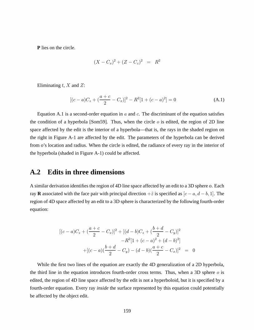
P lies on the circle.

(X − Cx)2 + (Z − Cz)

2 = R2

Eliminating t, X and Z:

[(c− a)Cz + (a + c

2− Cx)]

2 −R2[1 + (c− a)2] = 0 (A.1)

Equation A.1 is a second-order equation in a and c. The discriminant of the equation satisfies

the condition of a hyperbola [Som59]. Thus, when the circle o is edited, the region of 2D line

space affected by the edit is the interior of a hyperbola—that is, the rays in the shaded region on

the right in Figure A-1 are affected by the edit. The parameters of the hyperbola can be derived

from o’s location and radius. When the circle is edited, the radiance of every ray in the interior of

the hyperbola (shaded in Figure A-1) could be affected.

A.2 Edits in three dimensions

A similar derivation identifies the region of 4D line space affected by an edit to a 3D sphere o. Each

ray R associated with the face pair with principal direction +z is specified as [c− a, d− b, 1]. The

region of 4D space affected by an edit to a 3D sphere is characterized by the following fourth-order

equation:

[(c− a)Cz + (a+ c

2− Cx)]

2 + [(d− b)Cz + (b+ d

2− Cy)]

2

−R2[1 + (c− a)2 + (d− b)2]

+[(c− a)(b+ d

2− Cy)− (d− b)(

a+ c

2− Cx)]

2 = 0

While the first two lines of the equation are exactly the 4D generalization of a 2D hyperbola,

the third line in the equation introduces fourth-order cross terms. Thus, when a 3D sphere o is

edited, the region of 4D line space affected by the edit is not a hyperboloid, but it is specified by a

fourth-order equation. Every ray insidethe surface represented by this equation could potentially

be affected by the object edit.

159

160

Bibliography

[ACS94] A Andrade, Joao Comba, and Jorge Stolfi. Affine arithmetic. In Interval, St. Peters-

burg, Russia, March 1994.

[AF84] John Amanatides and Alain Fournier. Ray casting using divide and conquer in screen

space. In Intl. Conf. on Engineering and Computer Graphics. Beijing, China, August

1984.

[AH95] Stephen J. Adelson and Larry F. Hodges. Generating exact ray-traced animation

frames by reprojection. IEEE Computer Graphics and Applications, 15(3):43–52,

May 1995.

[AK87] James Arvo and David Kirk. Fast ray tracing by ray classification. In Computer

Graphics (SIGGRAPH 1987 Proceedings), pages 196–205, July 1987.

[Ama84] John Amanatides. Ray tracing with cones. In Computer Graphics (SIGGRAPH 1984

Proceedings), pages 129–135, July 1984.

[Bad88] S. Badt, Jr. Two algorithms for taking advantage of temporal coherence in ray tracing.

The Visual Computer, 4(3):123–132, September 1988.

[BDT98] Kavita Bala, Julie Dorsey, and Seth Teller. Bounded-error interactive ray tracing.

Technical Report Laboratory for Computer Science TR-748, Massachusetts Institute

of Technology, August 1998.

[BDT99a] Kavita Bala, Julie Dorsey, and Seth Teller. Interactive ray-traced scene editing using

ray segment trees. In Tenth Eurographics Workshop on Rendering, pages 39–52, June

1999.

[BDT99b] Kavita Bala, Julie Dorsey, and Seth Teller. Radiance interpolants for accelerated

bounded-error ray tracing. July 1999.

161

[BL94] Robert D. Blumofe and Charles E. Leiserson. Scheduling multithreaded computations

by work stealing. In 35th Annual Symposium on Foundations of Computer Science

(FOCS ’94), pages 356–368, November 1994.

[Bli78] James F. Blinn. Simulation of wrinkled surfaces. In Computer Graphics (SIGGRAPH

’78 Proceedings), pages 286–292, August 1978.

[BM98] Mark R. Bolin and Gary Meyer. A perceptually based adaptive sampling algorithm.

In Computer Graphics (SIGGRAPH ’98 Proceedings), Annual Conference Series,

pages 299–310, August 1998.

[BP96] Normand Briere and Pierre Poulin. Hierarchical view-dependent structures for inter-

active scene manipulation. In Computer Graphics (SIGGRAPH 1996 Proceedings),

pages 83–90, August 1996.

[CALM97] Miguel Castro, Atul Adya, Barbara Liskov, and Andrew C. Myers. HAC: Hybrid

adaptive caching for distributed storage systems. In Symposium on Operating Systems

(SOSP) 1997, pages 102–115, Oct. 1997.

[CCD90] John Chapman, Thomas W. Calvert, and John Dill. Exploiting temporal coherence

in ray tracing. In Proceedings of Graphics Interface 1990, pages 196–204, Toronto,

Ontario, May 1990. Canadian Information Processing Society.

[CCD91] John Chapman, Thomas W. Calvert, and John Dill. Spatio-temporal coherence in ray

tracing. In Proceedings of Graphics Interface 1991, pages 101–108, Calgary, Alberta,

June 1991. Canadian Information Processing Society.

[Che90] Shenchang Eric Chen. Incremental radiosity: An extension of progressive radiosity

to an interactive image synthesis system. Computer Graphics (ACM SIGGRAPH ’90

Proceedings), 24(4):135–144, August 1990.

[Che97] C. Chevrier. A view interpolation technique taking into account diffuse and specular

inter-reflections. The Visual Computer, 13(7):330–341, 1997.

[CLF98] Emilio Camahort, Apostolos Lerios, and Donald Fussell. Uniformly sampled light

fields. In Ninth Eurographics Workshop on Rendering, June 1998.

[CLR90] T. Cormen, C. Leiserson, and R. Rivest. Introduction to Algorithms. MIT Press and

McGraw-Hill, Cambridge, MA, 1990.

162

[Coo84] Robert L. Cook. Shade trees. In Computer Graphics (SIGGRAPH 1984 Proceedings),

volume 18, pages 223–231, July 1984.

[Coo86] Robert L. Cook. Stochastic sampling in computer graphics. ACM Transactions on

Graphics, 5(1):51–72, January 1986.

[Cox69] H. S. M. Coxeter. Introduction to Geometry. John Wiley & Sons Inc., 1969.

[Cra98] Tony Cragg. Pillars of salt. Sculpture of Goodwood, 1998.

[CRMT91] Shenchang Eric Chen, Holly E. Rushmeier, Gavin Miller, and Douglass Turner. A

progressive multi-pass method for global illumination. In Computer Graphics (SIG-

GRAPH 1991 Proceedings), pages 165–74, July 1991.

[CT82] Robert Cook and Kenneth Torrance. A reflectance model for computer graphics. ACM

Transactions on Graphics, 1(1):7–24, January 1982.

[CW93] Michael Cohen and John R. Wallace. Radiosity and Realistic Image Synthesis. Aca-

demic Press Professional, Cambridge, MA, 1993.

[DB69] G. Dahlquist and A. Bjorck. Numerical Methods. Prentice-Hall, New Jersey, 1969.

[DB97] Paul Diefenbach and Norman Badler. Multi-pass pipeline rendering: Realism for

dynamic environments. In Proceedings of the 1997 Symposium on Interactive 3D

Graphics, pages 59–70, April 1997.

[DS97] George Drettakis and Francois X. Sillion. Interactive update of global illumination

using a line-space hierarchy. In Computer Graphics (SIGGRAPH ’97 Proceedings),

pages 57–64, August 1997.

[FI85] Akira Fujimoto and Kansei Iwata. Accelerated ray tracing. In Tosiyasu Kunii, editor,

Computer Graphics: Visual Technology and Art (Proceedings of Computer Graphics

Tokyo 1985), pages 41–65, Tokyo, 1985. Springer-Verlag.

[FPSG96] James A. Ferwerda, Sumant N. Pattanaik, Peter Shirley, and Donald P. Greenberg.

A model of visual adaptation for realistic image synthesis. In Computer Graphics

(SIGGRAPH ’96 Proceedings), pages 249–258, August 1996.

[FPSG97] James A. Ferwerda, Sumant N. Pattanaik, Peter Shirley, and Donald P. Greenberg. A

model of visual masking for computer graphics. In Computer Graphics (SIGGRAPH

’97 Proceedings), pages 143–152, August 1997.

163

[FST92] T. Funkhouser, C. Sequin, and S. Teller. Management of large amounts of data in in-

teractive building walkthroughs. In Proc. 1992 Workshop on Interactive 3D Graph-

ics, pages 11–20, 1992.

[FvD82] J.D. Foley and A. van Dam. Fundamentals of Interactive Computer Graphics.

Addison-Wesley, 1982.

[FvDFH90] James D. Foley, Andries van Dam, Steven K. Feiner, and John F. Hughes. Computer

Graphics, Principles and Practice. Addison-Wesley, Reading, Massachusetts, second

edition, 1990.

[FYT94] David Forsyth, Chien Yang, and Kim Teo. Efficient radiosity in dynamic environ-

ments. In Proceedings 5th Eurographics Workshop on Rendering, June 1994.

[Gar84] M. Gardner. The Sixth Book of Mathematical Games from Scientific American. Uni-

versity of Chicago Press, Chicago, IL, 1984.

[GGC97] X. Gu, S. Gortler, and M. Cohen. Polyhedral geometry and the two-plane parameter-

ization. In Eight Eurographics Workshop on Rendering, pages 1–12, June 1997.

[GGSC96] Steven Gortler, Radek Grzeszczuk, Richard Szeliski, and Michael Cohen. The Lumi-

graph. In Computer Graphics (SIGGRAPH ’96 Proceedings), pages 43–54, August

1996.

[Gla84] Andrew S. Glassner. Space subdivision for fast ray tracing. IEEE Computer Graphics

and Applications, 4(10):15–22, 1984.

[Gla88] Andrew S. Glassner. Spacetime ray tracing for animation. IEEE Computer Graphics

and Applications, 8(2):60–70, March 1988.

[Gla89] Andrew S. Glassner. An Introduction to Ray Tracing. Academic Press, London, 1989.

[Gla95] Andrew S. Glassner. Principles of Digital Image Synthesis. Morgan Kaufmann Pub-

lishers, Inc., San Francisco, CA, 1995.

[GSG90] David W. George, Francois X. Sillion, and Donald P. Greenberg. Radiosity Redis-

tribution for Dynamic Environments. IEEE Computer Graphics and Applications,

10(4):26–34, July 1990.

164

[GTGB84] Cindy M. Goral, Kenneth E. Torrance, Donald P. Greenberg, and Bennett Battaile.

Modeling the interaction of light between diffuse surfaces. In Computer Graphics

(SIGGRAPH ’84 Proceedings), pages 213–222, July 1984.

[Guo98] Baining Guo. Progressive radiance evaluation using directional coherence maps. In

Computer Graphics (SIGGRAPH 1998 Proceedings), pages 255–266, August 1998.

[Han75] E. R. Hansen. A generalized interval arithmetic. In Interval Mathematics: Proceed-

ings of the International Symposium, pages 7–18, Karlsruhe, West Germany, May

1975. Springer-Verlag. Also published in Lecture Notes in Computer Science Vol-

ume 29.

[HH84] Paul S. Heckbert and Pat Hanrahan. Beam tracing polygonal objects. In Computer

Graphics (SIGGRAPH 1984 Proceedings), pages 119–127, July 1984.

[HSA91] Pat Hanrahan, David Salzman, and Larry Aupperle. A rapid hierarchical radiosity

algorithm. In Computer Graphics (SIGGRAPH ’91 Proceedings), pages 197–206,

July 1991.

[HTSG91] Xiao D. He, Kenneth E. Torrance, Francois X. Sillion, and Donald P. Greenberg.

A comprehensive physical model for light reflection. In Computer Graphics (SIG-

GRAPH 1991 Proceedings), pages 175–86, July 1991.

[HW91] E. Haines and J. Wallace. Shaft culling for efficient ray-traced radiosity. In Proc. 2nd

Eurographics Workshop on Rendering, May 1991.

[Jan86] Frederik W. Jansen. Data structures for ray tracing. In L. R. A. Kessener, F. J. Pe-

ters, and M. L. P. van Lierop, editors, Data Structures for Raster Graphics. Springer-

Verlag, New York, 1986.

[Jev92] David Jevans. Object space temporal coherence for ray tracing. In Proceedings of

Graphics Interface 1992, pages 176–183, Toronto, Ontario, May 1992. Canadian In-

formation Processing Society.

[LH96] Mark Levoy and Pat Hanrahan. Light field rendering. In Computer Graphics (SIG-

GRAPH ’96 Proceedings), pages 31–42, August 1996.

[LL76] L. D. Landau and E. M. Lifshitz. Course of Theoretical Physics: Mechanics.

Butterworth-Heinemann, 1976.

165

[LR98] Daniel Lischinski and Ari Rappoport. Image-based rendering for non-diffuse syn-

thetic scenes. In Rendering Techniques 1998, pages 301–314, June 1998.

[LSG94] Dani Lischinski, Brian Smits, and Donald P. Greenberg. Bounds and error estimates

for radiosity. In Computer Graphics (SIGGRAPH ’94 Proceedings), pages 67–74,

July 1994.

[MB95] Leonard McMillan and Gary Bishop. Plenoptic modeling: An image-based rendering

system. In Computer Graphics (SIGGRAPH ’95 Proceedings), August 1995.

[MH92] Koichi Murakami and Katsuhiko Hirota. Incremental ray tracing. In K. Bouatouch

and C. Bouville, editors, Photorealism in Computer Graphics. Springer-Verlag, 1992.

[MMB97] William Mark, Leonard McMillan, and Gary Bishop. Post-rendering 3d warping. In

Proceedings of the 1997 Symposium on Interactive 3D Graphics, pages 7–16, April

1997.

[Moo79] Ramon E. Moore. Methods and Applications of Interval Analysis. Studies in Applied

Mathematics (SIAM), Philadelphia, 1979.

[NDR95] Jeffry Nimeroff, Julie Dorsey, and Holly Rushmeier. A framework for global illumi-

nation in animated environments. In 6th Annual Eurographics Workshop on Render-

ing, pages 223–236, June 1995.

[OR98] Eyal Ofek and Ari Rappoport. Interactive relfections on curved objects. In Computer

Graphics (SIGGRAPH ’98 Proceedings), Annual Conference Series, pages 333–342,

August 1998.

[PFFG98] Sumant N. Pattanaik, James A. Ferwerda, Mark D. Fairchild, and Donald P. Green-

berg. A multiscale model of adaptation and spatial vision for realistic image display.

In Computer Graphics (SIGGRAPH ’98 Proceedings), Annual Conference Series,

pages 287–298, August 1998.

[PH97] Jovan Popovic and Hugues Hoppe. Progressive simplicial complexes. In Computer

Graphics (SIGGRAPH ’97 Proceedings), Annual Conference Series, pages 217–224,

August 1997.

[PLS97] F. Pighin, Dani Lischinski, and David Salesin. Progressive previewing of ray-traced

images using image-plane discontinuity meshing. In Rendering Techniques 1997,

pages 115–126, June 1997.

166

[PMS+99] Steven Parker, William Martin, Peter-Pike Sloan, Peter Shirley, Brian Smits, and

Chuck Hansen. Interactive ray tracing. In Interactive 3D Graphics (I3D), pages

119–126, April 1999.

[PPD98] Eric Paquette, Pierre Poulin, and George Drettakis. A light hierarchy for fast render-

ing of scenes with many lights. Eurographics ’98, 17(3), September 1998.

[Pra91] W. K. Pratt. Digital Image Processing (2nd Edition). John Wiley & Sons, Inc., 1991.

[PS89] James Painter and Kenneth Sloan. Antialiased ray tracing by adaptive progressive

refinement. In Computer Graphics (SIGGRAPH 1989 Proceedings), pages 281–288,

July 1989.

[Rot82] Scott D. Roth. Ray casting for modeling solids. Computer Graphics and Image

Processing, 18(2), February 1982.

[SAS92] Brian E. Smits, James R. Arvo, and David H. Salesin. An Importance-driven radiosity

algorithm. Computer Graphics (ACM SIGGRAPH ’92 Proceedings), 26(4):273–282,

July 1992.

[Som59] D.M.Y. Sommerville. Analytical Geometry of Three Dimensions. Cambridge Univer-

sity Press, 1959.

[SP89] Francois Sillion and Claude Puech. A general two-pass method integrating specular

and diffuse reflection. In Computer Graphics (SIGGRAPH 1989 Proceedings), pages

335–44, July 1989.

[SP94] F. Sillion and C. Puech. Radiosity and Global Illumination. Morgan Kaufmann

Publishers, Inc., San Francisco, CA, 1994.

[SS89] Carlo H. Sequin and Eliot K. Smyrl. Parameterized ray tracing. In Computer Graph-

ics (SIGGRAPH 1989 Proceedings), pages 307–314, July 1989.

[SS98] Cyril Soler and Francois X. Sillion. Fast calculation of soft shadow textures using

convolution. In Computer Graphics (SIGGRAPH ’98 Proceedings), pages 321–332,

August 1998.

[Tan87] A. S. Tanenbaum. Operating Systems: Design and Implementation. Prentice-Hall,

Inc., 1987.

167

[TBD96] Seth Teller, Kavita Bala, and Julie Dorsey. Conservative radiance interpolants for

ray tracing. In Seventh Eurographics Workshop on Rendering, pages 258–269, June

1996.

[TH93] Seth Teller and Pat Hanrahan. Global visibility algorithms for illumination computa-

tions. Computer Graphics (Proc. Siggraph ’93), pages 239–246, 1993.

[Tup96] Jeffrey Allen Tupper. Graphing equations with generalized interval arithmetic. Mas-

ter’s thesis, University of Toronto, 1996.

[War91] Gregory J. Ward. Adaptive shadow testing for ray tracing. In Second Eurographics

Workshop on Rendering, pages 11–20, 1991.

[War92] Gregory J. Ward. Measuring and modeling anisotropic reflection. In Computer

Graphics (SIGGRAPH 1992 Proceedings), pages 265–272, July 1992.

[War98] Gregory J. Ward. The Holodeck: a parallel ray-caching rendering system. In 2nd

Eurographics Workshop on Parallel Graphics and Visualization, 1998.

[WC88] Turner Whitted and Robert L. Cook. A comprehensive shading model. In Kenneth I.

Joy, Charles W. Grant, Nelson L. Max, and Lansing Hatfield, editors, Tutorial: Com-

puter Graphics: Image Synthesis, pages 232–43. Computer Society Press, Washing-

ton, DC, 1988.

[WCG87] John R. Wallace, Michael F. Cohen, and Donald P. Greenberg. A two-pass solution to

the rendering equation: A synthesis of ray tracing and radiosity methods. In Computer

Graphics (SIGGRAPH 1987 Proceedings), pages 311–20, July 1987.

[WDP99] Bruce Walter, George Drettakis, and Steven Parker. Interactive rendering using the

render cache. In Tenth Eurographics Workshop on Rendering, June 1999.

[WH92] Gregory Ward and Paul Heckbert. Irradiance gradients. In Rendering in Computer

Graphics (Proceedings of the Third Eurographics Workshop on Rendering). Springer-

Verlag, May 1992.

[WH98] H.-P. Seidel W. Heidrich, Ph. Slusallek. Sampling procedural shaders using affine

arithmetic. 17(3):158–176, July 1998.

[Whi80] Turner Whitted. An improved illumination model for shaded display. CACM,

23(6):343–349, 1980.

168

[WRC88] Gregory J. Ward, Francis M. Rubinstein, and Robert D. Clear. A ray tracing solution

for diffuse interreflection. In Computer Graphics (SIGGRAPH 1988 Proceedings),

pages 85–92, August 1988.

169