Embed Size (px)
Citation preview
RADIATION PHYSICS FOR PERSONNEL AND ENVIRONMENTAL PROTECTION
FERMILAB REPORT TM-1834
Revision 9B, May 2007
J. Donald Cossairt Fermi National Accelerator Laboratory
Presented at Sessions of the U. S. PARTICLE ACCELERATOR SCHOOL
ii
ACKNOWLEDGMENTS
This text is dedicated to my wife Claudia, and our children, Joe and Sally, who provided me with love, cheerfulness, and support during the initial preparation of these materials. I acknowledge the encouragement of John Peoples, Jr. and A. Lincoln Read to initially participate in the U. S. Particle Accelerator School. The support of my teaching in the USPAS by Mel Month, S. Y. Lee, Helmut Wiedemann, and Bill Griffing has been sincerely appreciated. Members of the Fermilab Environment, Safety and Health Section have greatly assisted me during the preparation and revision of these materials. Alex Elwyn deserves special recognition for his helpful advice during the preparation of this text and, indeed, during his entire distinguished career at Fermilab in which he, in so many ways, has been my mentor both in science and in our mutual hobby of photography. Kamran Vaziri’s careful reading of various editions of this text has also been of singular help. Nancy Grossman, Kamran Vaziri, Vernon Cupps, Reginald Ronningen (National Superconducting Cyclotron Laboratory at Michigan State University), Scott Schwahn (Thomas Jefferson National Accelerator Facility), and Sayed Rokni (Stanford Linear Accelerator Center) have provided me with very constructive criticism in connection with their assistance in presenting these materials to students in the USPAS. Others at Fermilab whose comments have been helpful are Dave Boehnlein, Kathy Graden, Paul Kesich, Elaine Marshall, Wayne Schmitt, Alan Wehmann, and Sam Childress. This work hopefully continues the great legacy of the late Miguel Awschalom. The original version of this text was presented as part of a course taught at the session of the U. S. Particle Accelerator School held at Florida State University in January 1993. Subsequently, the material was further refined and presented as a course at Fermilab in the spring of 1993 and autumn of 1994. The course has been part of the curriculum at USPAS sessions held under the auspices of Duke University (January 1995), The University of California, Berkeley (January 1997), Vanderbilt University (January 1999), Rice University (January 2001), Indiana University (January 2003), The University of Wisconsin, Madison (June 2004), and Arizona State University (January 2006). It will be presented under the auspices of Michigan State University in June 2007. It was presented in a series of lectures at Brookhaven National Laboratory in April 2005. Comments received from the many students who have endured the presentations have been very helpful in the continued development of this course. This publication is a compilation of the work of numerous people and it is hoped that the reference citations lead the reader to the original work of those individuals who have developed this field of applied physics. Over the years, I have been greatly enriched by being personally acquainted with many of these fine scientists. Notable among these in no particular order of prominence are the late Bill Swanson, the late Wade Patterson, Ralph Thomas, Geoffrey Stapleton, Graham Stevenson, Nikolai Mokhov, Ralph Nelson, James Liu, Vaclav Vylet, Theodore Jenkins, Keran O’Brien, Manfred Höfert, Anthony Sullivan, and Klaus Tesch.
J. Donald Cossairt
May 2007
iii
PREFACE
The advancement of particle accelerators is now well into its ninth decade, or second century if Röntgen’s x-ray tube is properly considered to be a particle accelerator. This field of human endeavor has achieved maturity but not stagnation. Accelerators now pervade nearly every facet of both modern scientific research and everyday life. They are utilized in virtually all branches of science ranging from the frontiers of particle and nuclear physics to engineering, chemistry, biology, geology, and the environmental sciences. Very important practical applications of accelerators are now found in many industrial applications and even in agriculture. The prominent and longstanding contribution to medicine is well-known as community hospitals of moderate size now utilize accelerators extensively. Indeed, particle accelerators are by far the type of “radiological” installation most commonly encountered by members of the public. The historical development of accelerator radiation physics has accompanied that of the machines themselves and has been well described by Patterson and Thomas (Pa94). A stated goal of the U. S. Particle Accelerator School (USPAS) is to provide “quality education in beam physics and associated accelerator technology”. It is therefore quite proper that the USPAS continues to include a course on accelerator radiation physics in its curriculum. Those who develop, operate, and utilize the accelerators of the future will be able to do this far more effectively if the associated radiological hazards are better understood and mitigated. To that end, the content of this textbook has been selected and developed. The intent is to address the major elements of radiation physics issues that are encountered at accelerators of all particle types and energies. To do this, some topics not commonly thought to be within the domain of “health physics” such as charged particle optics, synchrotron radiation, hydrogeology, and meteorology are included along with the more familiar subjects that might be anticipated by the readers. The problem sets supplied with most of the chapters were developed to promote better understanding of the contents.
TABLE OF CONTENTS
iv
Chapter 1 Basic Radiation Physics Concepts and Units of Measurement 1.1 Introduction 1 1.2 Review of Units, Physical Constants, and Material Properties 1 1.2.1 Radiation Physics Terminology and Units 1 1.2.2 Physical Constants and Atomic and Nuclear Properties 8 1.3 Summary of Relativistic Relationships 11 1.4 Energy Loss by Ionization and Multiple Coulomb Scattering 12 1.4.1 Energy Loss by Ionization 12 1.4.2 Multiple Coulomb Scattering 18 1.5 Radiological Standards 19 Problems 20 Chapter 2 General Considerations of Radiation Fields at Accelerators 2.1 Introduction 21 2.2 Primary Radiation Fields At Accelerators-General Considerations 21 2.3 Theory of Radiation Transport 23 2.3.1 General Considerations of Radiation Transport 23 2.3.2 The Boltzmann Equation 24 2.4 The Monte Carlo Method 26 2.4.1 General Principles of the Monte Carlo Technique 26 2.4.2 Monte Carlo Example; A Sinusoidal Angular Distribution of Beam Particles 28 2.5 Review of Magnetic Deflection and Focussing of Charged Particles 31 2.5.1 Magnetic Deflection of Charged Particles 31 2.5.2 Magnetic Focussing of Charged Particles 33 Problems 40 Chapter 3 Prompt Radiation Fields Due to Electrons 3.1 Introduction 41 3.2 Unshielded Radiation Produced by Electron Beams 41 3.2.1 Dose Equivalent Rate in a Direct Beam of Electrons 41 3.2.2 Bremsstrahlung 42 3.2.3 Synchrotron Radiation 47 3.2.4 Neutrons 49 3.2.4.1 Giant Photonuclear Resonance Neutrons 49 3.2.4.2 Quasi-Deuteron Neutrons 51 3.2.4.3 Neutrons Associated with the Production of Other Particles 52 3.2.5 Muons 52
3.2.6 Summary of Unshielded Radiation Produced by Electron Beams 54
3.3 The Electromagnetic Cascade-Introduction 55
TABLE OF CONTENTS
v
3.4 The Electromagnetic Cascade Process 58 3.4.1 Longitudinal Shower Development 59 3.4.2 Lateral Shower Development 62 3.5 Shielding of Hadrons Produced by the Electromagnetic Cascade 64 3.5.1 Neutrons 64 3.5.2 High Energy Particles 65 Problems 67 Chapter 4 Prompt Radiation Fields Due to Protons and Ions 4.1 Introduction 69 4.2 Radiation Production by Proton Accelerators 69 4.2.1 The Direct Beam; Radiation Hazards and Nuclear Interactions 69 4.2.2 Neutrons (and Other Hadrons at High Energies) 69 4.2.2.1 Eo < 10 MeV 71 4.2.2.2 10 < Eo < 200 MeV 71 4.2.2.3 200 MeV < Eo < 1 GeV; ("Intermediate" Energy) 74 4.2.2.4 Eo > 1 GeV ("High" Energy Region) 74 4.2.3 Sullivan's Formula 77 4.2.4 Muons 79 4.3 Primary Radiation Fields at Ion Accelerators 80 4.3.1 Light Ions (Ion Mass Number A < 5) 80 4.3.2 Heavy Ions (Ions with A > 4) 81 4.4 Hadron (Neutron) Shielding for Low Energy Incident Protons
(Eo < 15 MeV) 85 4.5 Limiting Attenuation at High Energy 88 4.6 Intermediate and High Energy Shielding-The Hadronic Cascade 90 4.6.1 The Hadronic Cascade from a Conceptual Standpoint 90 4.6.2 A Simple One-Dimensional Model 93 4.6.3 A Semiempirical Method, the Moyer Model for a Point Source 96 4.6.4 The Moyer Model for a Line Source 100 4.7 The Use of Monte Carlo Shielding Codes for Hadronic Cascades 102 4.7.1 Examples of Results of Monte Carlo Calculations 102 4.7.2 General Comments on Monte Carlo Star-to-Dose Conversions 106 4.7.3 Shielding Against Muons at Proton Accelerators 108 Problems 113 Chapter 5 Low Energy Prompt Neutron Radiation Phenomena 5.1 Introduction 116 5.2 Transmission of Photons and Neutrons Through Penetrations 116 5.2.1 Albedo Coefficients 116 5.2.1.1 Usage of Photon Albedo Coefficients 119 5.2.2 Neutron Attenuation in Labyrinths-General Considerations 121 5.2.3 Attenuation in First Leg of Rectilinear Penetrations or in Straight
Penetrations 122
TABLE OF CONTENTS
vi
5.2.4 Attenuation in Second and Successive Legs of Rectilinear Penetrations 126 5.2.5 Attenuation in Curved Tunnels 131 5.2.6 Attenuation Beyond the Exit 131 5.2.7 Determination of the Source Factor 133 5.3 Skyshine 134 5.3.1 Simple Parameterizations 134 5.3.2 A Somewhat More Rigorous Treatment 136 5.3.3 Examples of Experimental Verifications 140 Problems 144 Chapter 6 Shielding Materials and Neutron Energy Spectra 6.1 Introduction 145 6.2 Discussion of Shielding Materials Commonly Used at Accelerators 145 6.2.1 Earth 145 6.2.2 Concrete 146 6.2.3 Other Hydrogenous Materials 147 6.2.3.1 Polyethylene and Other Materials That Can Be Borated 147 6.2.3.2 Water, Wood, and Paraffin 148 6.2.4 Iron 148 6.2.5 High Atomic Number Materials (Lead, Tungsten, and Uranium) 149 6.2.6 Miscellaneous Materials (Beryllium, Aluminum, and Zirconium) 150 6.3 Neutron Energy Spectra Outside of Shields 150 6.3.1 General Considerations 150 6.3.2 Example of Neutron Spectra Due to Incident Electrons 151 6.3.3 Examples of Neutron Spectra Due to Low and Intermediate Energy Protons 153 6.3.4 Examples of Neutron Spectra Due to High Energy Protons 153 6.3.5 Leakage of Low Energy Neutrons Through Iron Shielding 160 6.3.6 Neutron Spectra Due to Ions 163 6.3.7 Neutron Fluence and Dosimetry 165 Chapter 7 Induced Radioactivity in Accelerator Components 7.1 Introduction 167 7.2 Fundamental Principles of Induced Radioactivity 167 7.3 Activation of Components at Electron Accelerators 169 7.3.1 General Phenomena 169 7.3.2 Results for Electrons at Low Energies 172 7.3.3 Results for Electrons at High Energies 175 7.4 Activation of Components at Proton and Ion Accelerators 180 7.4.1 General Phenomena 180 7.4.2 Methods of Systematizing Activation Due to High Energy Hadrons 188

TABLE OF CONTENTS
vii
7.4.2.1 Gollon's Rules of Thumb 192 7.4.3 The Utilization of Monte Carlo Star Densities in Activation Calculations 199 7.4.4 Uniform Irradiation of the Walls of an Accelerator Enclosures 202 Problems 205 Chapter 8 Induced Radioactivity in Environmental Media 8.1 Introduction 206 8.2 Airborne Radioactivity 206 8.2.1 Production 206 8.2.2 Accounting for Ventilation 207 8.2.3 Propagation of Airborne Radionuclides in the Environment 209 8.2.3.1 Propagation of Airborne Radioactivity - Tall Stacks 210 8.2.3.2 Propagation of Airborne Radioactivity - Short Stacks 212 8.2.4 Radiation Protection Standards for Airborne Radioactivity 213 8.2.5 Production of Airborne Radionuclides at Electron Accelerators 217 8.2.6 Production of Airborne Radionuclides at Proton Accelerators 219 8.3 Water and Geological Media Activation 220 8.3.1 Water Activation at Electron Accelerators 220 8.3.2 Water and Geological Media Activation at Proton Accelerators 222 8.3.2.1 Water Activation 222 8.3.2.2 Geological Media Activation 222 8.3.3 Regulatory Standards 226 8.3.4 The Propagation of Radionuclides Through Geological Media 228 Problems 235 Chapter 9 Radiation Protection Instrumentation at Accelerators 9.1 Introduction 237 9.2 Counting Statistics 237 9.3 Special Considerations for Accelerator Environments 240 9.3.1 Large Range of Flux Densities, Absorbed Dose Rates, etc. 240 9.3.2 Possible Large Instantaneous Values of Flux Densities, Absorbed Dose Rates, etc. 240 9.3.3 Large Energy Domain of Neutron Radiation Fields 240 9.3.4 Presence of Mixed Radiation Fields 240 9.3.5 Directional Sensitivity 241 9.3.6 Sensitivity to Features of the Accelerator Environment Other Than Ionizing Radiation 241 9.4 Standard Instruments and Dosimeters 241 9.4.1 Ionization Chambers 241 9.4.2 Geiger-Müller Detectors 245 9.4.3 Thermoluminescent Dosimeters (TLDs) 246 9.4.4 Nuclear Track Emulsions 247
TABLE OF CONTENTS
viii
9.4.5 Track Etch Dosimeters 247 9.4.6 CR-39 Dosimeters 247 9.4.7 Bubble Detectors 248 9.5 Specialized Detectors 248 9.5.1 Thermal Neutron Detectors 248 9.5.1.1 Boron-10 250 9.5.1.2 Lithium-6 251 9.5.1.3 Helium-3 251 9.5.1.4 Cadmium 253 9.5.1.5 Silver 253 9.5.2 Moderated Neutron Detectors 253 9.5.2.1 Spherical Moderators, Bonner Spheres, and Related Detectors 254 9.5.2.2 Long Counters 262 9.5.3 Activation Detectors 263 9.5.4 Fission Counters 266 9.5.5 Proton Recoil Counters 267 9.5.6 TEPCs and LET Spectrometry 268 9.5.7 The Recombination Chamber Technique 269 9.5.8 Counter Telescopes 273 Problems 275 Appendix A Summary Descriptions of Commonly Used Monte Carlo Codes 277 Appendix B Expanded Discussion of Synchrotron Radiation 281 B.1 General Discussion of the Phenomenon 281 B.2 Insertion Devices 284 B.3 Radiation Protection Issues Specific to Synchrotron Radiation Facilities 288 B.3.1 Operating Modes 288 B.3.2 Gas Bremsstrahlung - Straight Ahead 290 B.3.3 Gas Bremsstrahlung - Secondary Photons 291 B.3.4 Gas Bremsstrahlung Neutron Production Rates 293 B.3.5 Importance of Ray Tracing 295 Appendix C Examples of Results of Star Density Calculations Using CASIM 296 C.1 Results for Solid CONCRETE Cylinders 297 C.2 Restuls for Solid IRON Cylinders 299 C.3 Results for 1 TeV Protons Incident on Pipes and Magnets 301 References 303 Index 324
CHAPTER 1 BASIC RADIATION PHYSICS CONCEPTS AND UNITS OF MEASUREMENT
1
1.1 Introduction In this chapter, our discussion begins by reviewing the standard terminology of radiation physics. The most important physical and radiological quantities and the system of units by which they are measured are introduced. Due to its importance at most accelerators, the results of the special theory of relativity are reviewed. The energy loss by ionization and the multiple Coulomb scattering of charged particles is also summarized. 1.2 Review of Units, Terminology, Physical Constants, and Material Properties 1.2.1 Radiation Physics Terminology and Units In order to develop an understanding of accelerator radiation physics, it is necessary to introduce the prominent quantities of importance and the units by which they are measured that are commonly used in accelerator radiation protection. Over the years various systems of units have been employed. Presently, there is a slow migration toward the use of the Système Internationale (SI) units. However, the practitioner needs to understand the interconnections of all of the units, both "customary" and SI, due to the diversity of usage found in the scientific literature and in government regulations, particularly in the U.S. energy: The unit of energy in common use when dealing with energetic particles is the
electron volt (eV). 1 eV is equal to 1.602 x 10⁻¹² ergs or 1.602 x 10⁻¹⁹ Joules. Multiples of these units in common use at accelerators are the keV (103 eV), MeV (106 eV), GeV (109 eV), and TeV (1012 eV). In the scientific literature, particle energies are almost always measured in these energy units rather than in the SI equivalent (i.e., Joules). Also, nearly always, the "energy" of an accelerated particle refers to the kinetic energy (see section 1.3).
absorbed dose: Absorbed dose is the energy absorbed per unit mass of material. It is
usually denoted by the symbol D. The customary unit of absorbed dose is the rad while the Système Internationale (SI) unit of absorbed dose is the Gray. 1 rad is defined to be 100 ergs gram-1 or 6.24 x 10¹³ eV g-1. One Gray (Gy) is defined to be 1 J kg-1 and is thus 100 rads. A Gray, then, is equal to 6.24 x 10¹⁵ eV g-1. The concept of absorbed dose can be applied to any material. Thus it is commonly used to quantify both radiation exposures to human beings and the delivery of energy to materials and accelerator components where radiation damage is a consideration.
dose equivalent: This quantity has the same physical dimensions as absorbed dose. It is used to take into account the fact that different particle types have biological effects which are enhanced, per given absorbed dose, over those due to the standard reference particles which are 200 keV photons. It is usually denoted by the symbol H. The customary unit is the rem while the SI unit is the Sievert (Sv). One Sievert is equal to 100 rem. The concept of dose equivalent is relevant only to radiation exposures received by human beings. In recent years, variants of this quantity have been introduced such as “dose equivalent index” and “equivalent dose”. For the most part this text will ignore such subtleties.
CHAPTER 1 BASIC RADIATION PHYSICS CONCEPTS AND UNITS OF MEASUREMENT
2
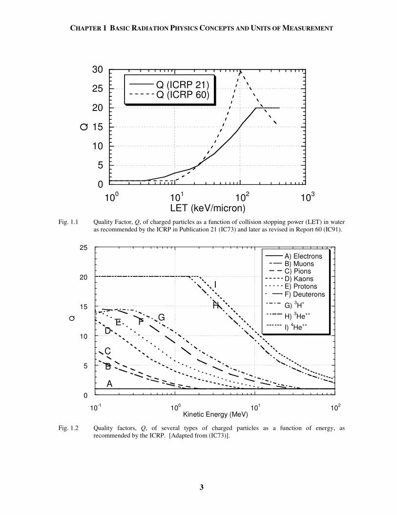
quality factor: This factor takes into account the relative enhancement in biological effects of various types of ionizing radiation. It is usually denoted by Q, and is used to connect H with D through the following equation:
H = QD. (1.1) Thus, H (rem) = QD (rads) or H (Sv) = QD (Gy). Q is dependent on both particle
type and energy and, thus, for any radiation field its value is an average over all components. It is formally defined to have a value of unity for 200 keV photons. Q ranges from unity for photons, electrons of most energies, and high energy muons to a value as large as 20 for α−particles (i.e.,4He nuclei) of a few MeV in kinetic energy. For neutrons, Q ranges from 2 to greater than 10. Although recent guidance by the International Council on Radiation Protection (ICRP) has recommended increased values of Q for neutrons (IC91), these increased values have yet to be adopted by regulatory authorities in the United States. Q is presently defined to be a function of linear energy transfer (LET), L. LET, approximately, is equivalent to stopping power, or rate of energy loss for charged particles and is conventionally expressed in units of keV µm-1 (see Section 1.4). All ionizing radiation ultimately manifests itself through charged particles so LET is, plausibly, a good measure of localized radiation damage.
The value of Q commonly used is an average over the spectrum of LET present,
weighted by the absorbed dose as a function of LET, D(L);
0
0
( ) ( )
( )
dLQ L D LQ
dLD L
∞
∞=
. (1.2)
Figures 1.1, 1.2, and 1.3 give the relationships between Q and LET and Q as a
function of particle energy for a variety of particles and energies. The results shown in Fig. 1.2 are based upon ionization due to the primary particles only. For particles subject to the strong (or nuclear) interaction, the inclusion of secondary particles produced at higher energies will result in increased values of Q as a function of energy. For example for protons Q rises to a value of 1.6 at 400 MeV and a value of 2.2 at 2000 MeV (Pa73) with secondary particles included. The subject of relating operationally useful values of Q to the existing knowledge of radiobiological effects is a complex one, discussed at length elsewhere (NC90). In general, it is preferred to use the dose equivalent per fluence conversion factors discussed below.
CHAPTER 1 BASIC RADIATION PHYSICS CONCEPTS AND UNITS OF MEASUREMENT
3
0
5
10
15
20
25
30
100 101 102 103
Q (ICRP 21)Q (ICRP 60)
Q
LET (keV/micron)
Fig. 1.1 Quality Factor, Q, of charged particles as a function of collision stopping power (LET) in water as recommended by the ICRP in Publication 21 (IC73) and later as revised in Report 60 (IC91).
0
5
10
15
20
25
10-1 100 101 102
A) ElectronsB) MuonsC) PionsD) KaonsE) ProtonsF) Deuterons
G) 3H+
H) 3He++
I) 4He++
Q
Kinetic Energy (MeV)
A
B
C
DE F G
H
I
Fig. 1.2 Quality factors, Q, of several types of charged particles as a function of energy, as
recommended by the ICRP. [Adapted from (IC73)].
CHAPTER 1 BASIC RADIATION PHYSICS CONCEPTS AND UNITS OF MEASUREMENT
4
0
2
4
6
8
10
12
10-8 10-6 10-4 10-2 100 102 104
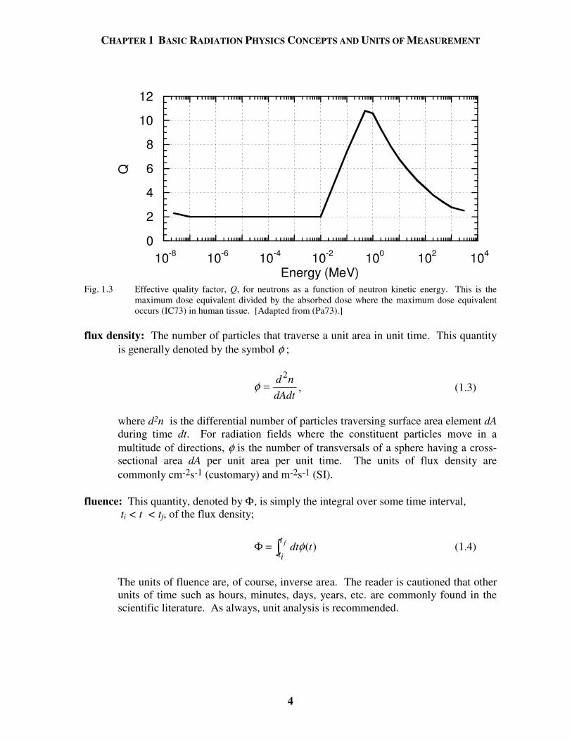
Q
Energy (MeV) Fig. 1.3 Effective quality factor, Q, for neutrons as a function of neutron kinetic energy. This is the
maximum dose equivalent divided by the absorbed dose where the maximum dose equivalent occurs (IC73) in human tissue. [Adapted from (Pa73).]
flux density: The number of particles that traverse a unit area in unit time. This quantity
is generally denoted by the symbol φ ;
φ = d ndAdt
2, (1.3)
where d2n is the differential number of particles traversing surface area element dA
during time dt. For radiation fields where the constituent particles move in a multitude of directions, φ is the number of transversals of a sphere having a cross-sectional area dA per unit area per unit time. The units of flux density are commonly cm-2s-1 (customary) and m-2s-1 (SI).
fluence: This quantity, denoted by Φ, is simply the integral over some time interval, ti < t < tf, of the flux density;
( )ft
tidt tφΦ = (1.4)
The units of fluence are, of course, inverse area. The reader is cautioned that other units of time such as hours, minutes, days, years, etc. are commonly found in the scientific literature. As always, unit analysis is recommended.
CHAPTER 1 BASIC RADIATION PHYSICS CONCEPTS AND UNITS OF MEASUREMENT
5
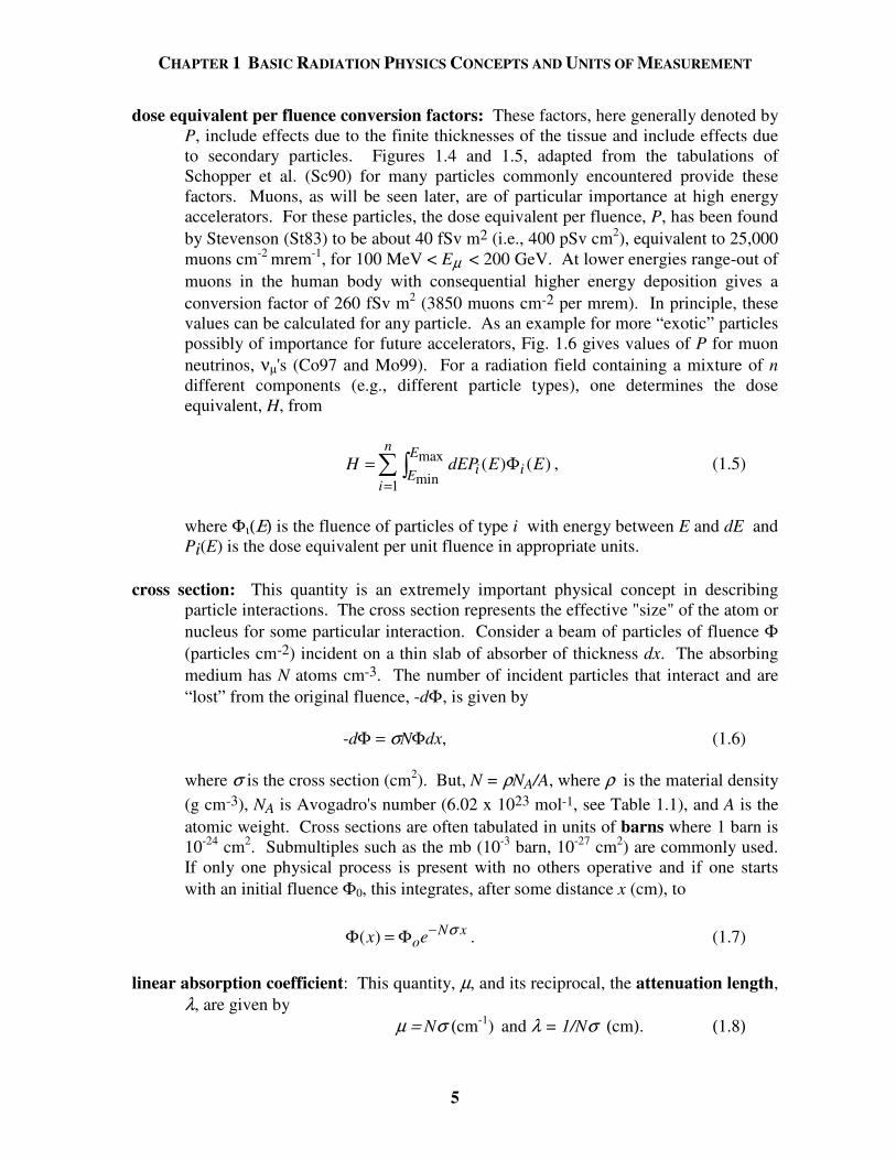
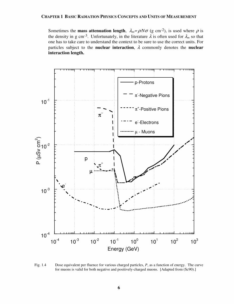
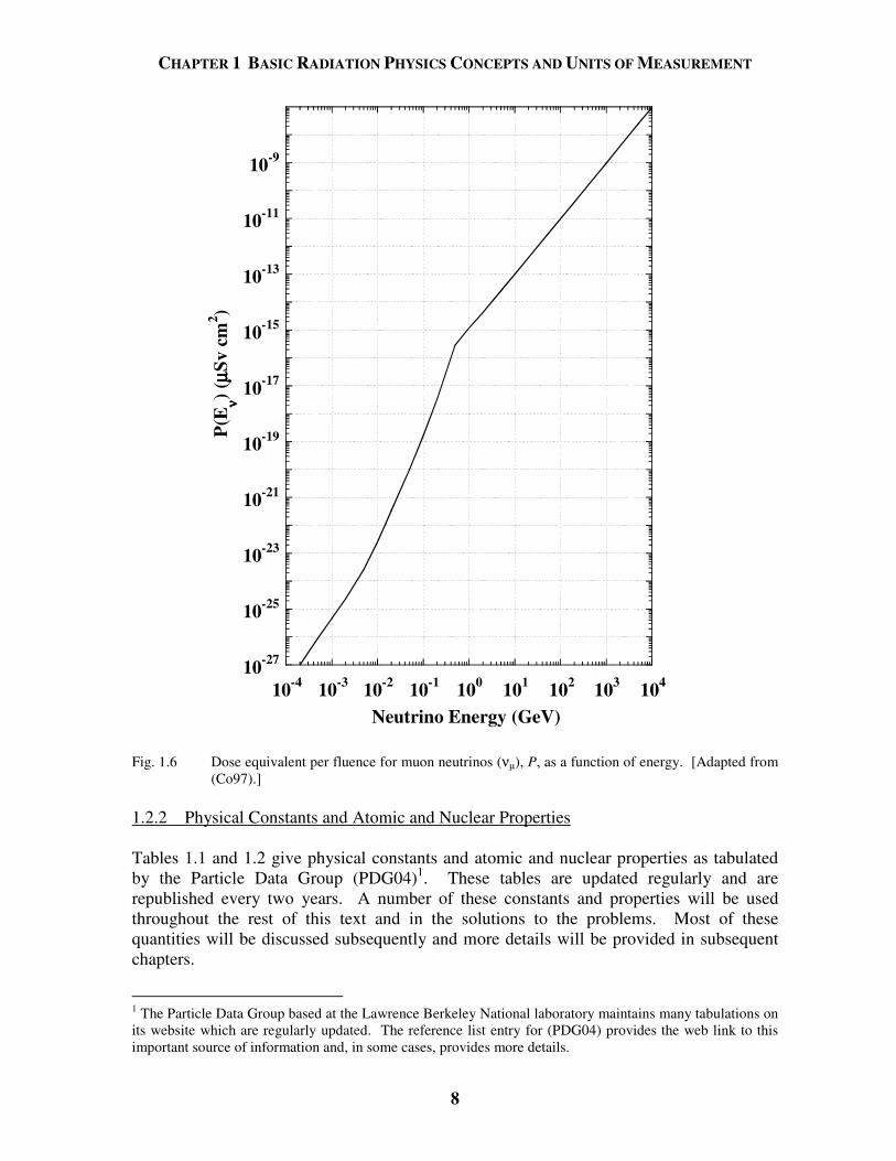
dose equivalent per fluence conversion factors: These factors, here generally denoted by P, include effects due to the finite thicknesses of the tissue and include effects due to secondary particles. Figures 1.4 and 1.5, adapted from the tabulations of Schopper et al. (Sc90) for many particles commonly encountered provide these factors. Muons, as will be seen later, are of particular importance at high energy accelerators. For these particles, the dose equivalent per fluence, P, has been found by Stevenson (St83) to be about 40 fSv m2 (i.e., 400 pSv cm2), equivalent to 25,000 muons cm-2 mrem-1, for 100 MeV < Eµ < 200 GeV. At lower energies range-out of muons in the human body with consequential higher energy deposition gives a conversion factor of 260 fSv m2 (3850 muons cm-2 per mrem). In principle, these values can be calculated for any particle. As an example for more “exotic” particles possibly of importance for future accelerators, Fig. 1.6 gives values of P for muon neutrinos, νµ's (Co97 and Mo99). For a radiation field containing a mixture of n different components (e.g., different particle types), one determines the dose equivalent, H, from
max
min1( ) ( )
n Ei iE
iH dEP E E
== Φ , (1.5)
where Φι(Ε) is the fluence of particles of type i with energy between E and dE and
Pi(E) is the dose equivalent per unit fluence in appropriate units. cross section: This quantity is an extremely important physical concept in describing
particle interactions. The cross section represents the effective "size" of the atom or nucleus for some particular interaction. Consider a beam of particles of fluence Φ (particles cm-2) incident on a thin slab of absorber of thickness dx. The absorbing medium has N atoms cm-3. The number of incident particles that interact and are “lost” from the original fluence, -dΦ, is given by
-dΦ = σNΦdx, (1.6) where σ is the cross section (cm2). But, N = ρNA/A, where ρ is the material density
(g cm-3), NA is Avogadro's number (6.02 x 10²³ mol-1, see Table 1.1), and A is the atomic weight. Cross sections are often tabulated in units of barns where 1 barn is 10-24 cm2. Submultiples such as the mb (10-3 barn, 10-27 cm2) are commonly used. If only one physical process is present with no others operative and if one starts with an initial fluence Φ0, this integrates, after some distance x (cm), to
( ) N xox e σ−Φ = Φ . (1.7)
linear absorption coefficient: This quantity, µ, and its reciprocal, the attenuation length,
λ, are given by µ = Nσ (cm-1) and λ = 1/Nσ (cm). (1.8)
CHAPTER 1 BASIC RADIATION PHYSICS CONCEPTS AND UNITS OF MEASUREMENT
6
Sometimes the mass attenuation length, λm= ρ/Nσ (g cm-2), is used where ρ is the density in g cm-3. Unfortunately, in the literature λ is often used for λm so that one has to take care to understand the context to be sure to use the correct units. For particles subject to the nuclear interaction, λ commonly denotes the nuclear interaction length.
10-4
10-3
10-2
10-1
10-4 10-3 10-2 10-1 100 101 102 103
p-Protons
π--Negative Pions
π+-Positive Pions
e--Electrons
µ - Muons
P (µ
Sv
cm2 )
Energy (GeV)
p
π−
π+
e-
µµ
π−
Fig. 1.4 Dose equivalent per fluence for various charged particles, P, as a function of energy. The curve
for muons is valid for both negative and positively-charged muons. [Adapted from (Sc90).]
CHAPTER 1 BASIC RADIATION PHYSICS CONCEPTS AND UNITS OF MEASUREMENT
7
10-8
10-7
10-6
10-5
10-4
10-3
10-2
10-11 10-10 10-9 10-8 10-7 10-6 10-5 10-4 10-3 10-2 10-1 100 101 102
Photons
Neutrons
P (µ
Sv
cm2 )
Energy (GeV)
Fig. 1.5 Dose equivalent per fluence for photons and neutrons, P, as a function of energy. [Adapted from (Sc90).]
CHAPTER 1 BASIC RADIATION PHYSICS CONCEPTS AND UNITS OF MEASUREMENT
8
10-27
10-25
10-23
10-21
10-19
10-17
10-15
10-13
10-11
10-9
10-4 10-3 10-2 10-1 100 101 102 103 104
P(E
νν νν) (µµ µµS
v cm
2 )
Neutrino Energy (GeV)
Fig. 1.6 Dose equivalent per fluence for muon neutrinos (νµ), P, as a function of energy. [Adapted from (Co97).]
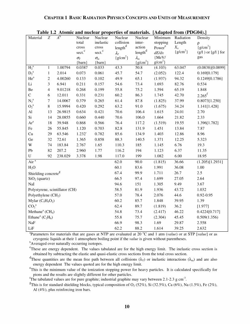
1.2.2 Physical Constants and Atomic and Nuclear Properties Tables 1.1 and 1.2 give physical constants and atomic and nuclear properties as tabulated by the Particle Data Group (PDG04)1. These tables are updated regularly and are republished every two years. A number of these constants and properties will be used throughout the rest of this text and in the solutions to the problems. Most of these quantities will be discussed subsequently and more details will be provided in subsequent chapters.
1 The Particle Data Group based at the Lawrence Berkeley National laboratory maintains many tabulations on its website which are regularly updated. The reference list entry for (PDG04) provides the web link to this important source of information and, in some cases, provides more details.
CHAPTER 1 BASIC RADIATION PHYSICS CONCEPTS AND UNITS OF MEASUREMENT
9
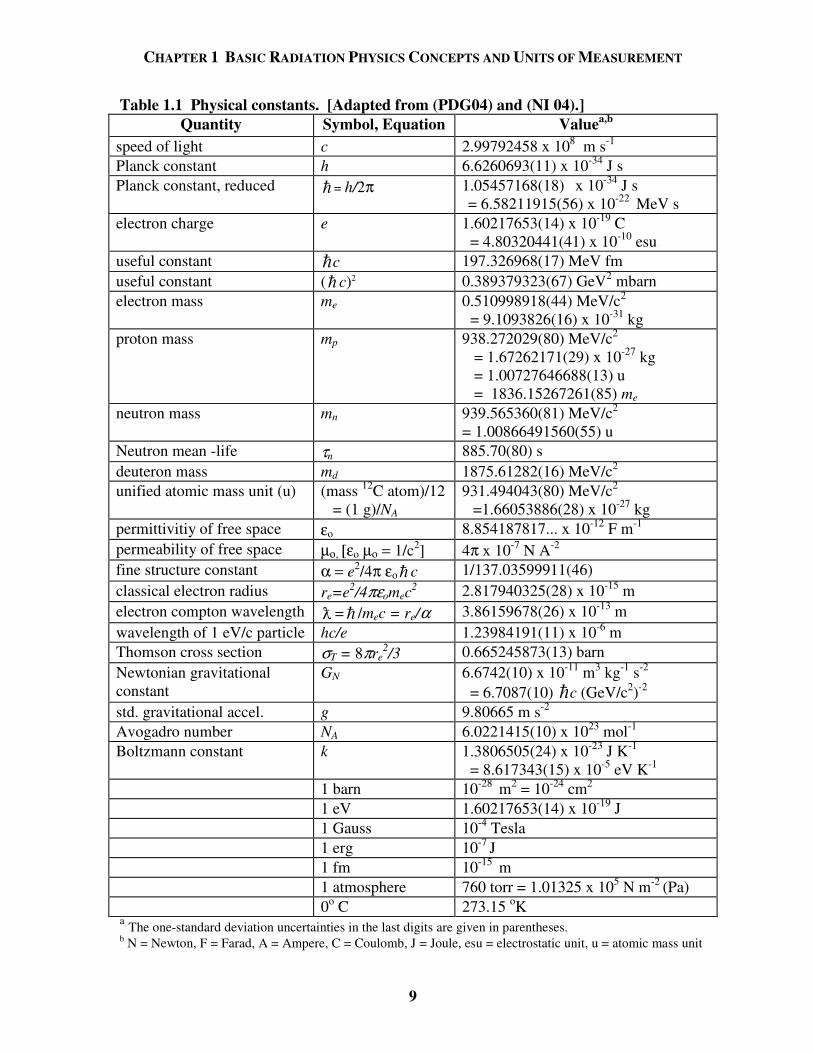
Table 1.1 Physical constants. [Adapted from (PDG04) and (NI 04).] Quantity Symbol, Equation Valuea,b
speed of light c 2.99792458 x 10⁸ m s-1 Planck constant h 6.6260693(11) x 10-34 J s Planck constant, reduced = h/2π 1.05457168(18) x 10-34 J s
= 6.58211915(56) x 10-22 MeV s electron charge e 1.60217653(14) x 10-19 C
= 4.80320441(41) x 10-10 esu useful constant c 197.326968(17) MeV fm useful constant ( c)2 0.389379323(67) GeV2 mbarn electron mass me 0.510998918(44) MeV/c2
= 9.1093826(16) x 10-31 kg proton mass mp 938.272029(80) MeV/c2
= 1.67262171(29) x 10-27 kg = 1.00727646688(13) u = 1836.15267261(85) me
neutron mass mn 939.565360(81) MeV/c2 = 1.00866491560(55) u
Neutron mean -life τn 885.70(80) s deuteron mass md 1875.61282(16) MeV/c2 unified atomic mass unit (u) (mass 12C atom)/12
= (1 g)/NA 931.494043(80) MeV/c2
=1.66053886(28) x 10-27 kg permittivitiy of free space εo 8.854187817... x 10-12 F m-1 permeability of free space µο, [εo µο = 1/c2] 4π x 10-7 N A-2 fine structure constant α = e2/4π εo c 1/137.03599911(46) classical electron radius re=e2/4πεomec2 2.817940325(28) x 10-15 m electron compton wavelength = /mec = re/α 3.86159678(26) x 10-13 m wavelength of 1 eV/c particle hc/e 1.23984191(11) x 10-6 m Thomson cross section σT = 8πre
2/3 0.665245873(13) barn Newtonian gravitational constant
GN 6.6742(10) x 10-11 m3 kg-1 s-2 = 6.7087(10) c (GeV/c2)-2
std. gravitational accel. g 9.80665 m s-2 Avogadro number NA 6.0221415(10) x 1023 mol-1 Boltzmann constant k 1.3806505(24) x 10-23 J K-1
= 8.617343(15) x 10-5 eV K-1
1 barn 10-28 m2 = 10-24 cm2
1 eV 1.60217653(14) x 10-19 J 1 Gauss 10-4 Tesla 1 erg 10-7 J 1 fm 10-15 m 1 atmosphere 760 torr = 1.01325 x 10⁵ N m-2 (Pa) 0o C 273.15 oK a The one-standard deviation uncertainties in the last digits are given in parentheses. b N = Newton, F = Farad, A = Ampere, C = Coulomb, J = Joule, esu = electrostatic unit, u = atomic mass unit
CHAPTER 1 BASIC RADIATION PHYSICS CONCEPTS AND UNITS OF MEASUREMENT
10
Table 1.2 Atomic and nuclear properties of materials. [Adapted from (PDG04).] Material Z Ab
Nuclear total cross sect.c σT barn
Nuclear inelastic cross sect.c σin
barn
Nuclear collision lengthd
λT g/cm2
Nuclear inter-action lengthd
λin g/cm2
Minimum stopping Powere
dE/dx
MeV/ g/cm2
Radiation Length Xo
g/cm2
Density
ρ g/cm3 (g/l ) or [g/l ] for gas
H2a 1 1.00794 0.0387 0.033 43.3 50.8 (4.103) 63.047 (0.0838)[0.0899]
D2a 1 2.014 0.073 0.061 45.7 54.7 (2.052) 122.4 0.169[0.179]
Hea 2 4.00260 0.133 0.102 49.9 65.1 (1.937) 94.32 0.1249[0.1786] Li 3 6.941 0.211 0.157 54.6 73.4 1.693 82.76 0.534 Be 4 9.01218 0.268 0.199 55.8 75.2 1.594 65.19 1.848 C 6 12.011 0.331 0.231 60.2 86.3 1.745 42.70 2.265f N2
a 7 14.0067 0.379 0.265 61.4 87.8 (1.825) 37.99 0.8073[1.250] O2
a 8 15.9994 0.420 0.292 63.2 91.0 (1.675) 34.24 1.141[1.428] Al 13 26.9815 0.634 0.421 70.6 106.4 1.615 24.01 2.70 Si 14 28.0855 0.660 0.440 70.6 106.0 1.664 21.82 2.33 Ara 18 39.948 0.868 0.566 76.4 117.2 (1.519) 19.55 1.396[1.782] Fe 26 55.845 1.120 0.703 82.8 131.9 1.451 13.84 7.87 Cu 29 63.546 1.232` 0.782 85.6 134.9 1.403 12.86 8.96 Ge 32 72.61 1.365 0.858 88.3 140.5 1.371 12.25 5.323 W 74 183.84 2.767 1.65 110.3 185 1.145 6.76 19.3 Pb 82 207.2 2.960 1.77 116.2 194 1.123 6.37 11.35 U 92 238.029 3.378 1.98 117.0 199 1.082 6.00 18.95 Air a 62.0 90.0 (1.815) 36.66 (1.205)[1.2931] H2O 60.1 83.6 1.991 36.08 1.00
Shielding concreteg 67.4 99.9 1.711 26.7 2.5 SiO2 (quartz) 66.5 97.4 1.699 27.05 2.64 NaI 94.6 151 1.305 9.49 3.67 Polystyrene, scintillator (CH) 58.5 81.9 1.936 43.72 1.032 Polyethylene (CH2) 57.0 78.4 2.076 44.6 0.92-0.95 Mylar (C5H4O2) 60.2 85.7 1.848 39.95 1.39 CO2
a 62.4 89.7 (1.819) 36.2 [1.977] Methanea (CH4) 54.8 73.4 (2.417) 46.22 0.4224[0.717] Ethanea (C2H6) 55.8 75.7 (2.304) 45.45 0.509(1.356) NaF 66.9 98.3 1.69 29.87 2.558 LiF 62.2 88.2 1.614 39.25 2.632 aParameters for materials that are gases at NTP are evaluated at 20 oC and 1 atm (value) or at STP [value] or as
cryogenic liquids at their 1 atmosphere boiling point if the value is given without parentheses. bAveraged over naturally occurring isotopes. cThese are energy dependent. The values tabulated are for the high energy limit. The inelastic cross section is
obtained by subtracting the elastic and quasi-elastic cross sections from the total cross section. dThese quantities are the mean free path between all collisions (λT) or inelastic interactions (λin) and are also
energy dependent The values quoted are for the high energy limit. eThis is the minimum value of the ionization stopping power for heavy particles. It is calculated specifically for
pions and the results are slightly different for other particles. fThe tabulated values are for pure graphite; industrial graphite may vary between 2.1-2.3 g cm-3. gThis is for standard shielding blocks, typical composition of O2 (52%), Si (32.5%), Ca (6%), Na (1.5%), Fe (2%),
Al (4%), plus reinforcing iron bars.
CHAPTER 1 BASIC RADIATION PHYSICS CONCEPTS AND UNITS OF MEASUREMENT
11
1.3 Summary of Relativistic Relationships The results of the special theory of relativity are quite evident at most accelerators. In this section, the important conclusions are reviewed. The rest energy, Wo, of a particle of rest mass mo is given by Wo = moc2 , (1.9) where c is the velocity of light. The total energy in free space, W, is given by
2
2 221
oo
m cW mc m cγ
β= = =
−, with
2
1,
1o
WW
γβ
= =−
(1.10)
where β = v/c and v is the velocity of the particle in a given frame of reference. The relationship between the quantities β and γ is obvious. Similarly, the relativistic mass, m, of a particle moving at velocity β is given by
21
oo
mm mγ
β= =
−. (1.11)
The kinetic energy, E, is E = W - Wo = (m - mo)c2 and (1.12)
β = −
1 02
W
W . (1.13)
The momentum, p, of a particle in terms of its relativistic mass, m, and velocity, v, is;
22 2
2
1 11 ( 2 )o o
o o oo
Wm Wp mv m c c W W E E W
m c W c cγ β
= = = − = − = +
, (1.14)
so that at high energies, p ≈ E/c ≈ W/c while at low energies (E << Wo) one has the familiar nonrelativistic p2 ≈ 2(Wo/c2)E = 2moE. It is usually most convenient to work in a system of units where energy is in units of eV, MeV, etc. Velocities are then expressed in units of the speed of light (β ), momenta are expressed as energy divided by c (e.g., MeV/c, etc.), and masses are expressed as energy divided by c2 (e.g., MeV/c2, etc.). In these units, the total energy, W, and the relativistic mass, m, are equivalent. One thus avoids the explicit inclusion of numerical values for c, or c2. The decay length at a given velocity of a particle with a finite meanlife (at rest), τ, is given by γβcτ, where relativistic time dilation is taken into account by inclusion of the factor γ.
CHAPTER 1 BASIC RADIATION PHYSICS CONCEPTS AND UNITS OF MEASUREMENT
12
The product of the speed of light and the meanlife, cτ, is often tabulated. The decay length is the mean distance traveled by a particle in vacuum prior to its decay. This length must be distinguished from that called the decay path. The decay path represents a distance in space in which a given particle is allowed to decay with no or minimal competition from other effects such as scattering or absorption. Thus, the decay length is determined by the basic physics of the decay process while the decay path is defined by the physical configuration of the accelerator components present. 1.4 Energy Loss by Ionization and Multiple Coulomb Scattering 1.4.1 Energy Loss by Ionization For moderately relativistic particles, the mean rate of energy loss, the stopping power, is given approximately by
2 2 22 2 2 2
2
214 ln
2e
A e e
m cdE ZN r m c z
dx A Iγ β δπ β
β
− = − −
(MeV cm2g-1), (1.15)
where NA is Avogadro's number (atoms mol-1), Z and A are the atomic number and weight of the material traversed, z is the charge state of the projectile in units of electron charge, me and re are the rest mass and "classical radius" of the electron (see Table 1.1), and I is the ionization constant. For Z > 1, I ≈ 16Z0.9 eV while for diatomic hydrogen (H2), I = 19 eV. β and γ are as defined in Section 1.3. δ is a small correction factor that can be approximated by 2 lnγ. Substituting constants, for I in eV;
6 2 22 2
2
1 1.022 100.3071 ln
2dE Z
zdx A I
γ β δββ
×− = − −
(MeV cm2g-1). (1.16)
This is the stopping power2 due to ionization, the process in which a charged particle transfers its energy to atomic electrons in the absorbing medium. In these units, the dependence upon the absorbing material is slowly-varying given the fact that I appears only in the logarithmic term and the ratio Z/A ranges between 0.4 to 0.5 over most of the periodic table for stable nuclides. Thus, for a given projectile charge z the value of the stopping power, dE/dx, is most strongly dependent on β. A broad minimum is found at a value of γ = 3.2. At this value of γ, the particles are said to be minimum ionizing and the corresponding minimum stopping powers are listed in Table 1.2. The absorption of the energy of charged particles by ionization is characterized by a parameter called the range, R, in material. The range is the length of the path followed by the particle while it is losing its energy. Simplistically one might think that one could
2 The argument of the logarithmic term of Eqs (1.15) and (1.16) must be dimensionless. Hence, the rest energy of the electron, mec
2, and I must be in the same units (e.g., both in eV). These equations are found in Phys Rev. D45 (1992) S1, the 1992 edition of reference (PDG04). This version of these equations is somewhat simpler than, but equivalent to, that found in (PDG04) and thus is adopted for use here.
CHAPTER 1 BASIC RADIATION PHYSICS CONCEPTS AND UNITS OF MEASUREMENT
13
calculate the value of R by a numerical integration of the reciprocal of the stopping power. However, as the particles lose energy by ionization and thus slow down, other effects at very low energies become important that are not included in Eq. (1.15). It is prudent, therefore, to consult explicit tabulations to determine the particle ranges. For charged particles much more massive than electrons, the trajectory through the material to first approximation is a straight line modified only by multiple Coulomb scattering (see Section 1.4.2) since the mass of the moving particle is so much larger than the mass of the atomic electrons. For a moving electron, the range is the sum of many divergent line segments through the material since its mass is identical to that of the atomic electrons encountered with the consequence that the individual angular deflections are much larger. As shall be seen in Section 3.2.2, for electrons the loss of energy in matter due to the radiation of photons increases rapidly with electron kinetic energy and becomes much more important than the ionization stopping power or the range at relatively low energies. The situation is also different for particles such as protons that participate in the nuclear interaction. For these particles, as the kinetic energy of the particle increases, the absorption of the particles through strong interaction processes has a high probability of absorbing the particles prior to their depositing all of their energy by ionization. This will be discussed further in Section 4.2.1. Figures 1.7 and 1.8 give stopping power and range values as a function of momentum or energy for common high energy particles and for some light ions, respectively. Detailed tables of the values of stopping power and ranges for many heavy ions have been given by Northcliffe and Schilling (No70). Also, the Monte Carlo computer code SRIM is currently easily obtained and may be used to generate similar tables as well as do simulations of protons or heavy charged ions interacting with elemental or compound materials (Zi96). For muons (µ's) the situation is rather unique. The muon rest energy is 105.66 MeV, its meanlife τ = 2.1970 x 10⁻⁶ s, and the meanlife times the speed of light is cτ = 658.65 m. Due to their large rest mass compared to that of the electron and the fact that these particles, to first order, do not participate in the strong (nuclear) interaction, muons tend to penetrate long distances in matter without being absorbed by other mechanisms. Muons, due to their heavier masses, are also far less susceptible to radiative effects. Thus, over a very large energy domain, the principal energy loss mechanism is that of ionization. This, as shall be seen later, makes the shielding of muons matter of considerable importance at high energy accelerators. The range-energy relation of muons is given in Fig. 1.9. At high energies (Eµ
> 100 GeV), the distribution of the ranges of individual muons about the mean range, called the range straggling, becomes severe (Va87). Also, above a muon energy of several hundred GeV, radiative losses begin to dominate such that the stopping power, dE/dx, is given by (PDG 04)
( ) ( )dE
a E b E Edx
− = + , (1.17)
where a(E) is the collisional ionization energy loss [from Eq. (1.16), approximately 0.002 GeV cm2g-1], and b(E) is the radiative coefficient for E in GeV. The latter parameter separated into contributions from the important physical mechanisms is plotted in Fig. 1.10.
CHAPTER 1 BASIC RADIATION PHYSICS CONCEPTS AND UNITS OF MEASUREMENT
14
Fig. 1.7 A. Mean ionization stopping power in various media as a function of particle momenta.
Radiative effects are not included. B. Ionization range of heavy charged particles in various media. The abscissa of these plots are scaled to the ratio of particle momenta, p, to particle rest mass, M. [Reproduced from (PDG04).]
CHAPTER 1 BASIC RADIATION PHYSICS CONCEPTS AND UNITS OF MEASUREMENT
15
Fig. 1.8 Stopping power (top) and ranges (bottom) for protons in three different materials. These curves can be used for other incident particles by taking their atomic number, z, and mass, m (in atomic mass units), into account. The incident energy is thus expressed as the specific kinetic energy, E/m. The curves are approximately correct except at the very lowest energies where charge exchange effects can be important. The results are most valid for projectile mass, m < 4 [Adapted from (En66).]
CHAPTER 1 BASIC RADIATION PHYSICS CONCEPTS AND UNITS OF MEASUREMENT
16
10-1
100
101
102
103
104
100 101 102 103 104
Water
Aluminum
Earth
Iron
Lead
Ran
ge (
met
ers)
Energy (GeV)
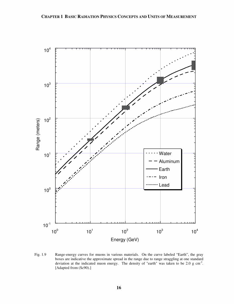
Fig. 1.9 Range-energy curves for muons in various materials. On the curve labeled “Earth”, the gray
boxes are indicative the approximate spread in the range due to range straggling at one standard deviation at the indicated muon energy. The density of "earth" was taken to be 2.0 g cm-2. [Adapted from (Sc90).]
CHAPTER 1 BASIC RADIATION PHYSICS CONCEPTS AND UNITS OF MEASUREMENT
17
0
2
4
6
8
10
10 0 10 1 10 2 10 3 10 4
b(E
) (g-1
cm
2 ) x 1
0-6
M uon Energy (G eV)
bto ta l
bpair
bbrem sstrahlung
bnuclear
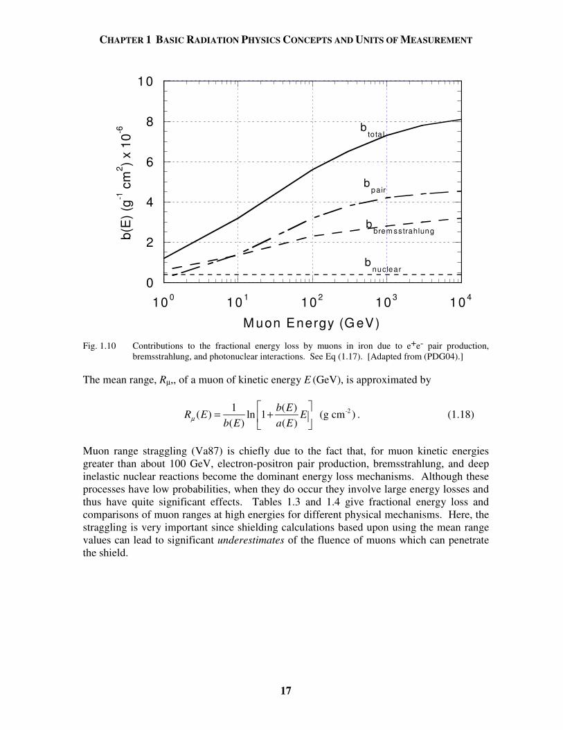
Fig. 1.10 Contributions to the fractional energy loss by muons in iron due to e+e- pair production,
bremsstrahlung, and photonuclear interactions. See Eq (1.17). [Adapted from (PDG04).] The mean range, Rµ,, of a muon of kinetic energy E (GeV), is approximated by
-21 ( )( ) ln 1 (g cm )
( ) ( )b E
R E Eb E a Eµ
= +
. (1.18)
Muon range straggling (Va87) is chiefly due to the fact that, for muon kinetic energies greater than about 100 GeV, electron-positron pair production, bremsstrahlung, and deep inelastic nuclear reactions become the dominant energy loss mechanisms. Although these processes have low probabilities, when they do occur they involve large energy losses and thus have quite significant effects. Tables 1.3 and 1.4 give fractional energy loss and comparisons of muon ranges at high energies for different physical mechanisms. Here, the straggling is very important since shielding calculations based upon using the mean range values can lead to significant underestimates of the fluence of muons which can penetrate the shield.

CHAPTER 1 BASIC RADIATION PHYSICS CONCEPTS AND UNITS OF MEASUREMENT
18
Table 1.3 Fractional energy loss of muons in soil (ρρρρ = 2.0 g cm-3). The fractions of the total energy loss due to the four dominant energy loss mechanisms are given. [Adapted from (Va87) and (Sc90).]
Energy
(GeV)
Ionization Bremsstrahlung Pair production Deep inelastic nuclear scattering
10 0.972 0.037 8.8 x 10⁻⁴ 9.7 x 10⁻⁴ 100 0.888 0.086 0.020 0.0093
1000 0.580 0.193 0.168 0.055 10,000 0.167 0.335 0.388 0.110
Table 1.4 Comparison of muon ranges (meters) in heavy soil (ρρρρ = 2.24 g cm3). [Adapted from (Va87) and (Sc90).]
Energy Mean Ranges from dE/dx in Heavy Soil (meters)
(GeV) Mean Range (meters)
Standard Deviation (meters)
All Processes Coulomb Losses Only
Coulomb & Pair
Production Losses
10 22.8 1.6 21.4 21.5 21.5 30 63.0 5.6 60.3 61.1 60.8
100 188 23 183 193 188 300 481 78 474 558 574
1000 1140 250 1140 1790 1390 3000 1970 550 2060 5170 2930
10,000 3080 890 3240 16,700 5340 20,000 3730 1070
1.4.2 Multiple Coulomb Scattering Multiple Coulomb scattering from nuclei is an important effect in the transport of charged particles through matter. A charged particle traversing a medium is deflected by many small-angle scattering events and only occasionally by ones involving large-angle scattering. The small-angle scattering events are largely due to Coulomb scattering from nuclei so that the effect is called multiple Coulomb scattering. This simplification is not quite correct for hadrons since it ignores the contribution of strong interactions to multiple scattering. For purposes of discussion here, a Gaussian approximation adequately describes the distribution of deflection angles of the final trajectory compared with the incident trajectory for all charged particles. The distribution as a function of deflection angle, θ, is as follows:
2
20 0
( ) exp22
df d
θ θθ θθθ π
= −
. (1.19)
The mean width of the projected angular distribution,θο , on a particular plane is approximated by
CHAPTER 1 BASIC RADIATION PHYSICS CONCEPTS AND UNITS OF MEASUREMENT
19
13.6
1 0.038 lnoo o
z x xpc X X
θβ
= +
(radians) (1.20)
where z is the charge of the projectile in units of the charge of the electron, p is the particle momentum in MeV/c and x is the absorber thickness in the same units as the quantity Xo (PDG04). Xo is a material-dependent parameter, to be discussed further in Section 3.2.2 called the radiation length. This description of multiple Coulomb scattering has been validated for particles having momenta up to 200 GeV/c by Shen et al. (Sh79). The best values of the radiation length are probably those of Tsai (Ts74), the values tabulated in Table 1.2. A compact, approximate formula for calculating the value of Xo as a function of atomic number, Z, and atomic weight, A, of the material medium (PDG04) is
( )716.4
( 1) ln 287 /o
AX
Z Z Z=
+ (g cm-2) . (1.21)
Results obtained using this formula agree to those of Tsai within about 2.5 % for all elements except helium, where the result is about 5 % low. An alternative method of calculating Xo using different atomic wave functions is given by Seltzer and Berger (Se85). It provides results similar to those given by Eq. (1.21). 1.5 Radiological Standards While the discussion of radiological standards is not a topic of great emphasis in this text, some mention of it seems to be appropriate. Standards or limits on occupational and environmental exposure to ionizing radiation are now instituted worldwide. In general, individual nations, or sub-national entities, incorporate guidance provided by international or national bodies into their laws and regulations. The main international body that develops radiological standards is the International Commission on Radiation Protection (ICRP). Another international institution, the International Commission on Radiation Units and Measurements (ICRU), also is an important standards-setting institution. In the United States, the major national body chartered by the U. S. Congress is the National Council on Radiation Protection and Measurements (NCRP). Standards developed by these organizations are referenced in other chapters of this text. Of particular interest are the following References: (IC71), (IC73), (IC78), (IC87), (IC91), (NC77), (NC90), and (NC03). In the U.S. the U. S. Environmental Protection Agency (EPA) is the primary federal agency for establishing basic radiological requirements. These are further implemented by the U.S. Department of Energy (DOE) for its facilities, and by individual states. At present the U. S. Nuclear Regulatory Commission (NRC) does not regulate particle accelerators. However, certain aspects of state regulations pertaining to accelerators are reflective of general NRC requirements for radiation protection. The regulation of accelerator facilities varies considerably between individual states and some local jurisdictions, the authority having jurisdiction should be consulted to obtain an accurate understanding of applicable regulatory requirements.
CHAPTER 1 BASIC RADIATION PHYSICS CONCEPTS AND UNITS OF MEASUREMENT
20
Problems 1. a) Express 1 kilowatt (1 kW) of beam power in GeV s-1.
b) To how many singly charged particles per second does 1 ampere of beam current
correspond?
c) Express an absorbed dose of 1 Gy in GeV kg-1 of energy deposition.
2. Which has the higher quality factor, a 10 MeV (kinetic energy) α-particle or a 1 MeV neutron? Write down the quality factors for each particle.
3. Calculate the number of
12C and
238U atoms in a cubic centimeter of solid material.
4. Calculate the velocity and momenta of a 200 MeV electron, proton, iron ion, π+,
and µ+. The 200 MeV is kinetic energy and the answers should be expressed in units of the speed of light (velocity) and MeV/c (momenta). Iron ions have an isotope-averaged mass of 52021 MeV (A = 55.847 x 931.5 MeV/amu). The π+
mass is 140 MeV and the µ+ mass = 106 MeV. Do the same calculation for 20 GeV protons, iron ions, and muons. It is suggested that these results be presented in tabular form. Make general comments on the velocity and momenta of the particles at the two energies. (The table may help you notice any algebraic errors that you may have made.)
5. Calculate the mass stopping power of a 20 MeV electron (ionization only) and a
200 MeV proton in 28Si. 6. Calculate the fluence of minimum ionizing muons necessary to produce a dose
equivalent of 1 mrem assuming a quality factor = 1 and that tissue is equivalent to water for minimum ionizing muons. (Hint: use Table 1.2.) Compare with the results given in Fig. 1.4 for high energies.
CHAPTER 2 GENERAL CONSIDERATIONS OF RADIATION FIELDS AT ACCELERATORS
21
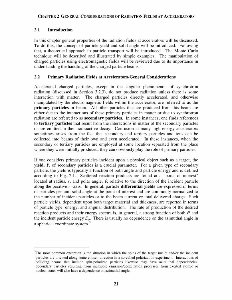
2.1 Introduction In this chapter general properties of the radiation fields at accelerators will be discussed. To do this, the concept of particle yield and solid angle will be introduced. Following that, a theoretical approach to particle transport will be introduced. The Monte Carlo technique will be described and illustrated by simple examples. The manipulation of charged particles using electromagnetic fields will be reviewed due to its importance in understanding the handling of the charged particle beams. 2.2 Primary Radiation Fields at Accelerators-General Considerations
Accelerated charged particles, except in the singular phenomenon of synchrotron radiation (discussed in Section 3.2.3), do not produce radiation unless there is some interaction with matter. The charged particles directly accelerated, and otherwise manipulated by the electromagnetic fields within the accelerator, are referred to as the primary particles or beam. All other particles that are produced from this beam are either due to the interactions of these primary particles in matter or due to synchrotron radiation are referred to as secondary particles. In some instances, one finds references to tertiary particles that result from the interactions in matter of the secondary particles or are emitted in their radioactive decay. Confusion at many high energy accelerators sometimes arises from the fact that secondary and tertiary particles and ions can be collected into beams of their own and even accelerated. In these instances, when the secondary or tertiary particles are employed at some location separated from the place where they were initially produced, they can obviously play the role of primary particles. If one considers primary particles incident upon a physical object such as a target, the yield, Y, of secondary particles is a crucial parameter. For a given type of secondary particle, the yield is typically a function of both angle and particle energy and is defined according to Fig. 2.1. Scattered reaction products are found at a "point of interest" located at radius, r, and polar angle, θ, relative to the direction of the incident particle along the positive z -axis. In general, particle differential yields are expressed in terms of particles per unit solid angle at the point of interest and are commonly normalized to the number of incident particles or to the beam current or total delivered charge. Such particle yields, dependent upon both target material and thickness, are reported in terms of particle type, energy, and angular distribution. The rate of production of the desired reaction products and their energy spectra is, in general, a strong function of both θ and the incident particle energy Eo. There is usually no dependence on the azimuthal angle in a spherical coordinate system.3
3The most common exception is the situation in which the spins of the target nuclei and/or the incident particles are oriented along some chosen direction in a so-called polarization experiment. Interactions of colliding beams that include spin-polarized particles likewise may have azimuthal dependencies. Secondary particles resulting from multipole emission/deexcitation processes from excited atomic or nuclear states will also have a dependence on azimuthal angle.
CHAPTER 2 GENERAL CONSIDERATIONS OF RADIATION FIELDS AT ACCELERATORS
22
θ
r
INCIDENT BEAM
Z-AXIS
POINT OF INTEREST
TARGET
Fig. 2.1 Conceptual interaction of incident beam with material (target) which produces radiation at the point of interest located at polar coordinates (r, θ).
In principle, the particle yield could be obtained directly from differential cross sections for given incident particle kinetic energy E;
( , )d Ed
σ θΩ
,
where σ (E,θ) is the cross section as a function of energy and angle and Ω is the solid angle into which the secondary particles are directed. For example, Y could, in principle be obtained from an integration of this cross section as it varies with energy while the incident particle loses energy in passing through the target material.
Calculations of the radiation field that directly use the cross sections are often not practical because targets hit by beam are not really “thin”. Thus one cannot ignore energy loss or secondary interactions in the target. Furthermore, the knowledge of cross sections at all energies is often incomplete with the unfortunate result that one cannot always integrate over θ and E to get the total yield. For many applications, the details of the angular distributions of total secondary particle yield, dY(θ )/dΩ, and the angular dependence of the emitted particle energy spectrum, d2Y(E,θ)/dEdΩ, are very important.
CHAPTER 2 GENERAL CONSIDERATIONS OF RADIATION FIELDS AT ACCELERATORS
23
Often, the particle fluence is needed at a particular location at coordinates (r,θ ) from a known point source of beam loss while the angular distributions of dY/dΩ are generally expressed in units of particles/(steradian-incident particle). To obtain the total fluence Φ (θ ) [e.g., particles/(cm2.incident particle)], or differential fluence dΦ(E ,θ)/dE [e.g., particles/(cm2.MeV.incident particle)] at a given distance r (cm) at a specified angle θ from such a point source4, one must simply multiply the yield values by r -2:
2
1 ( )( )
dYr d
θθΦ =Ω
and 2
2
( , ) 1 ( , )d E d Y EdE r dEd
θ θΦ =Ω
. (2.1)
Given the fact that secondary, as well as primary, particles can create radiation fields, it is quite obvious that the transport of particles through space and matter can become a very complex matter. In the following section, the advanced techniques for handling these issues are described. 2.3 Theory of Radiation Transport The theoretical material in this section is largely due to the work of O'Brien (OB80). It is included to show clearly the mathematical basis of the contents of shielding codes, especially those that use the Monte Carlo method. Vector notation is used in this section. 2.3.1 General Considerations of Radiation Transport Stray and direct radiations at any location are distributed in particle type, direction, and energy. To determine the amount of radiation present for radiation protection purposes one must assign a magnitude to this multidimensional quantity. This is done by forming a double integral over energy and direction of the product of the flux density and an approximate dose equivalent per unit fluence conversion factor, summed over particle type;
04
( , ) ( , , , ) ( )i i
i
dH x td dE f x E t P E
dt π
∞= Ω Ω
, (2.2)
where the summation index i is over the various particle types, Ω
is the direction vector of particle travel,
x is the coordinate vector of the point in space where the dose or dose
equivalent is to be calculated, E is the particle energy, t is time, and i is the particle type. Pi(E) is the dose equivalent per fluence conversion factor expressed as a function of energy and particle type for the ith particle. The inner integral is over all energies while the outer integral is over all spatial directions from which contributions to the radiation field at the location specified by
x originate. The result of the integration is ( ),dH x t dt
,
the dose equivalent rate at location x and time t. Values of Pi(E) are given in Figs. 1.4,
4 A point source is one in which the dimensions of the source are small compared with the distance to some other location of interest.
CHAPTER 2 GENERAL CONSIDERATIONS OF RADIATION FIELDS AT ACCELERATORS
24
1.5, and 1.6. The angular flux density, f x E ti ( , , , )
Ω , the number of particles of type i per unit area, per unit energy, per unit solid angle, per unit time at location
x , with a
energy E, at a time t, and traveling in a direction Ω is related to the total flux density,
( , )x tφ , by integrating over direction and particle energy;
04
( , ) ( , , , )ii
x t d dE f x E tπ
φ∞
= Ω Ω
. (2.3)
The angular flux density, f x E ti ( , , , )
Ω , is connected to the total fluence ( )xΦ by
integrating over a relevant interval of time (ti to tf ), as well as direction and energy;
04
( ) ( , , , )f
ii
i
t
tx d dE dt f x E t
π
∞Φ = Ω Ω
, (2.4)
and to the energy spectrum expressed as a flux density for particle type i at point x at
time t, ( , , )i x t Eφ , by
4
( , , ) ( , , , )i ix t E d f x E tπ
φ = Ω Ω
. (2.5)
To determine the proper dimensions and composition of a shield, the amount of radiation, expressed in terms of the dose or dose equivalent, which penetrates the shield and reaches locations of interest must be calculated. This quantity must be compared with the maximum permissible dose equivalent. If the calculated dose equivalent is too large, either the conditions associated with the source of the radiation or the physical properties of the shield must be changed. The latter could be a change in shield materials, dimensions, or both. If the shield cannot be adjusted, then the amount of beam loss allowed by the beam control instrumentation, the amount of residual gas in the vacuum system, or the amount of beam accelerated may have to be reduced. It is difficult and expensive, especially in the case of the larger accelerators, to alter permanent shielding or operating conditions if the determination of shielding dimensions and composition has not been done correctly. The methods for determining these quantities have been investigated by a number of workers. The next section only summarizes the basics of this important work. 2.3.2 The Boltzmann Equation The primary tool for determining the amount of radiation reaching a given location is the stationary form of the Boltzmann equation (henceforth, simply the Boltzmann equation) which, when solved, yields the angular flux density, fi, the distribution in energy and angle for each particle type as a function of position and time. The angular flux density is then converted to dose equivalent rate by means of Eq. (2.2). This section describes the

CHAPTER 2 GENERAL CONSIDERATIONS OF RADIATION FIELDS AT ACCELERATORS
25
theory that yields the distribution of radiation in matter, and discusses some of the methods for extracting detailed numerical values for elements of this distribution such as particle flux, or related quantities, such as dose, activation or instrument response. The Boltzmann equation is a statement of all the processes that the particles of various types, including photons, that comprise the radiation field can undergo. A much more complete derivation and discussion has been given by O’Brien (OB80). This equation is an integral-differential equation describing the behavior of a dilute assemblage of corpuscles. It was derived by Ludwig Boltzmann in 1872 to study the properties of gases but applies equally to the behavior of those "corpuscles" which comprise ionizing radiation. This equation is a continuity equation of the angular flux density, fi, in phase space which is made up of the three space coordinates of Euclidian geometry, the three corresponding direction cosines, the kinetic energy, and the time. The density of radiation in a volume of phase space may change in the following five ways:
• uniform translation; where the spatial coordinates change, but the energy-angle coordinates remain unchanged;
• collisions; as a result of which the energy-angle coordinates change, but the
spatial coordinates remain unchanged, or the particle may be absorbed and disappear altogether;
• continuous slowing down; in which uniform translation is combined with
continuous energy loss;
• decay; where particles are changed through radioactive transmutation into particles of another kind; and
• introduction; involving the direct emission of a particle from a source into the
volume of phase space of interest: electrons or photons from radioactive materials, neutrons from an α-n emitter, the "appearance" of beam particles, or particles emitted from a collision at another (usually higher) energy.
Combining these five elements yields
( , , , )i i ij if x E t Q YΒ Ω = + , (2.6)
where the mixed differential and integral Boltzmann operator for particles of type i, iΒ , is given by
ii i i
Sd
Eσ ∂
Β = Ω ⋅∇ + + −∂
, (2.7)
CHAPTER 2 GENERAL CONSIDERATIONS OF RADIATION FIELDS AT ACCELERATORS
26
( )max
4
, ( , , )E
ij B ij B joj
Q d dE E E f x E tπ
σ′ ′ ′= Ω → Ω → Ω Ω ,
, (2.8)
and dcii
i i=
−1 2βτ β
. (2.9)
In Eq. (2.7): Yi is the number of particles of type i introduced by a source per unit area, time,
energy, and solid angle; σi is the absorption cross section for particles of type i. To be dimensionally
correct, this is actually the macroscopic cross section or linear absorption coefficient µ = Nσ as defined in Eq. (1.8);
di is the decay probability per unit flight path of radioactive particles (such as
muons or pions) of type i; Si is the stopping power for charged particles of type i (assumed to be zero for
uncharged particles); Qij is the "scattering-down" integral; the production rate of particles of type i with
a direction Ω
, an energy E at a location x , by collisions with nuclei or decay of
j-type particles having a direction Ω′
at a higher energy EB; σij is the doubly-differential inclusive cross section for the production of i-type
particles with energy E and a direction Ω
from nuclear collisions or decay of j-type particles with a direction EB and a direction Ω′
; and
βi is the velocity of a particle of type i divided by the speed of light c; and τi is the
mean- life of a radioactive particle of type i in the rest frame. This equation is obviously quite difficult to solve in general and special techniques have been devised to yield useful results. The Monte Carlo method is the most common method of approximate solution used in the field of radiation shielding. 2.4 The Monte Carlo Method 2.4.1 General Principles of the Monte Carlo Technique The Monte Carlo method is based on the use of random sampling to obtain the solution of the Boltzmann equation. It is one of the most useful methods for evaluating radiation
CHAPTER 2 GENERAL CONSIDERATIONS OF RADIATION FIELDS AT ACCELERATORS
27
hazards for realistic geometries that are generally quite difficult to characterize using analytic techniques (i.e., with equations in closed form). The calculation proceeds by constructing a series of trajectories, each segment of which is chosen at random from a distribution of applicable processes. In the simplest and most widely used form of the Monte Carlo technique, the so-called inverse transform method, a history is obtained by calculating travel distances between collisions and then sampling from distributions in energy and angle made up from the cross sections, ),( Ω→Ω′→
EEBijσ . (2.10)
The result of the interaction may be a number of particles of varying types, energies, and directions each of which will be followed in turn. The results of many histories will be tabulated, leading typically to some sort of mean and standard deviation. If p(x)dx is the differential probability of an occurrence at x + 1/2 dx in the interval, [a,b], then the integration
′′=x
axpxdxP )()( (2.11)
gives P(x), the cumulative probability that the event will occur in the interval [a, x]. The cumulative probability function is monotonically increasing with x and always satisfies the conditions P(a) = 0, P(b) = 1. If a random number R uniform on the interval [0, 1] is chosen, for example from a computer routine, the equation R = P(x) (2.12) corresponds to a random choice of the value of x, since the distribution function for the event P(x) can, in principle, be inverted as a unique one-to-one mapping;
x P R= −1( ) . (2.13) As a simple illustration, to determine when an uncharged particle undergoes a reaction in a one-dimensional system with no decays (d = 0), no competing processes (S = 0), and no "in-scattering" (Q = 0), one recognizes from Eqs. (1.6), (2.6), and (2.7) that a simple application of the Boltzmann equation is applicable; B iσΦ = Ω ⋅ ∇ + Φ
. (2.14)
This simple situation reduces to the following, taking in this discussion σi to be the macroscopic cross section otherwise denoted by Nσ in this text;
0d
Ndx
σΦΒΦ = + Φ = . (2.15)
CHAPTER 2 GENERAL CONSIDERATIONS OF RADIATION FIELDS AT ACCELERATORS
28
The solution to this equation is the familiar 0 exp( / )x λΦ = Φ − , (2.16) where λ = 1/Nσ as in Eq. (1.8). One can replace x/λ with r, the number of mean-free-paths the particle travels in the medium. The differential probability per unit mean-free-path for an interaction is given by p(r) = exp(-r) , (2.17)
with ]
0 0( ) exp( ) exp( ) 1 exp( )
rrP r dr r r r R′ ′ ′= − = − − = − − = . (2.18)
Selecting a random number, R, then determines a depth r that has the proper distribution. Of course, mathematically identical results apply to other processes described by an exponential function such as radioactive decay. In this simple situation, it is clear that one can solve the above for r as a function of R and thus obtain individual values of r from a corresponding set of random numbers. For many processes, an inversion this simple is not possible analytically. In those situations, other techniques exemplified by successive approximations and table look-up procedures must be employed. In a Monte Carlo calculation, the next sampling process might select which of several physical processes would occur. Another sampling might choose, for instance, the scattering of the particle being followed. Deflections by magnetic fields might be included as well as further particle production and/or decay. The Monte Carlo result is the number of times the event of interest occurred for the random steps through the relevant processes. As a counting process it has a counting uncertainty and the variance will tend to decrease as the square root of the number of calculations run on the computer. Thus high probability processes can be more accurately simulated than low probability processes such as passage through a thick shield in which the radiation levels are attenuated over many orders of magnitude. In modern calculations, sophisticated techniques are often employed which temporarily give enhanced probabilities to the low-probability events during the calculation in order to study them. The normal probabilities are restored at the end of the calculation by removing these so-called “weights” to obtain realistic results. It is by no means clear that the distributions obtained using the Monte Carlo method will be distributed according to the normal, or Gaussian distribution, so that a statistical test of the adequacy of the mean and standard deviation may be required. 2.4.2 Monte Carlo Example; A Sinusoidal Angular Distribution of Beam Particles Suppose one has a distribution of beam particles such as exhibited in Fig 2.2.

CHAPTER 2 GENERAL CONSIDERATIONS OF RADIATION FIELDS AT ACCELERATORS
29
0 0.2 0.4 0.6 0.8 1 1.2 1.4 1.6
dN/d
θ
θ (radians)
Fig. 2.2 Hypothetical angular distribution of particles obeying a distribution proportional to cos θ. For this distribution, p(θ ) = A cos θ for 0 < θ < π/2. Then, the fact that the integral of p(θ ) over the relevant interval 0 < θ < π/2 to get the cumulative probability P(θ = π/2) must be unity implies A =1 since
1sincos)2/(def2/
02/
0===
ππθθθπ AAdP . (2.19)
Thus, p(θ ) = cos θ. The cumulative probability, P(θ ), is then given by
θθθθθθθ θθθsinsincos)()( =′=′′=′′= ooo
dpdP . (2.20)
If R is a random number, then R = P(θ ) determines a unique value of θ ; hence
1sin ( ).Rθ −= (2.21)
One can perform a simple Monte Carlo calculation using, for example, 50 random numbers. To do this one should set up a table such as Table 2.1 that was generated using a particular set of such random numbers. One can set up a set of bins of successive ranges of θ -values. The second column is a "tally sheet" for collecting "events" in which a random number R results in a value of θ within the associated range of θ-values. θmid is the midpoint of the bin (0.1, 0.3,...). Column 4 is the normalized number in radians found from the following:
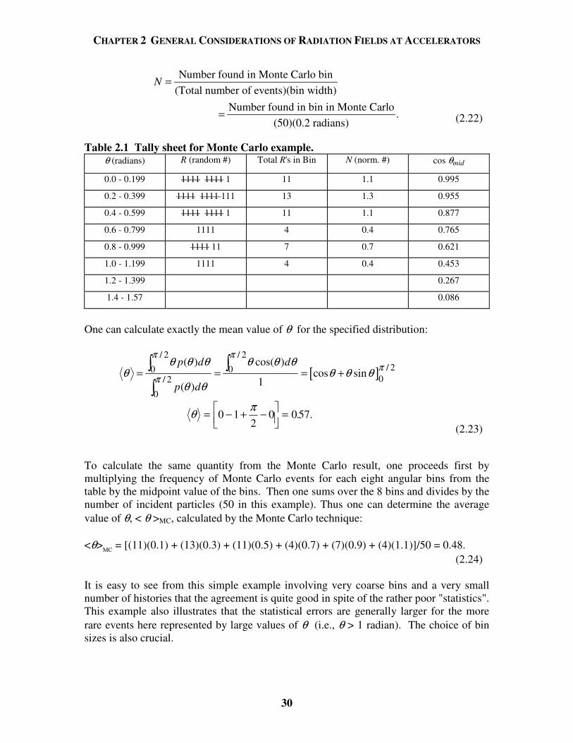
CHAPTER 2 GENERAL CONSIDERATIONS OF RADIATION FIELDS AT ACCELERATORS
30
Number found in Monte Carlo bin(Total number of events)(bin width)
Number found in bin in Monte Carlo .
(50)(0.2 radians)
N =
= (2.22)
Table 2.1 Tally sheet for Monte Carlo example. θ (radians) R (random #) Total R's in Bin N (norm. #) cos θmid
0.0 - 0.199 1111 1111 1 11 1.1 0.995
0.2 - 0.399 1111 1111 111 13 1.3 0.955
0.4 - 0.599 1111 1111 1 11 1.1 0.877
0.6 - 0.799 1111 4 0.4 0.765
0.8 - 0.999 1111 11 7 0.7 0.621
1.0 - 1.199 1111 4 0.4 0.453
1.2 - 1.399 0.267
1.4 - 1.57 0.086
One can calculate exactly the mean value of θ for the specified distribution:
[ ]/ 2 / 2
/ 20 00/ 2
0
( ) cos( )cos sin
1( )
p d d
p d
π ππ
π
θ θ θ θ θ θθ θ θ θ
θ θ= = = +
(2.23)
To calculate the same quantity from the Monte Carlo result, one proceeds first by multiplying the frequency of Monte Carlo events for each eight angular bins from the table by the midpoint value of the bins. Then one sums over the 8 bins and divides by the number of incident particles (50 in this example). Thus one can determine the average value of θ, < θ >MC, calculated by the Monte Carlo technique: <θ>MC = [(11)(0.1) + (13)(0.3) + (11)(0.5) + (4)(0.7) + (7)(0.9) + (4)(1.1)]/50 = 0.48. (2.24) It is easy to see from this simple example involving very coarse bins and a very small number of histories that the agreement is quite good in spite of the rather poor "statistics". This example also illustrates that the statistical errors are generally larger for the more rare events here represented by large values of θ (i.e., θ > 1 radian). The choice of bin sizes is also crucial.
θ π = − + −
= 0 1 2
0 0 57. .
CHAPTER 2 GENERAL CONSIDERATIONS OF RADIATION FIELDS AT ACCELERATORS
31
Practical Monte Carlo calculations generally involve the need to follow a huge number of histories. Early calculations of this type, such as the one reported by Wilson (Wi52), were made using devices such as "wheels of chance" and hand-tallying. The advent of digital computers has rendered this technique much more powerful. As the speed of computer processors has increased, the ability to model the physical effects in more detail and with ever improving statistical accuracy has resulted. In later chapters, results obtained using specific codes will be presented. Descriptions of the codes themselves, accurate as of this writing, are presented in Appendix A. The reader should be cautioned that most of these codes are being constantly improved and updated. The wisest practice in using them is to consult with the authors of the codes directly. 2.5 Review of Magnetic Deflection and Focussing of Charged Particles 2.5.1 Magnetic Deflection of Charged Particles Particle accelerators of all types operate by utilizing electromagnetic forces to accelerate deflect, and focus charged particles. These forces have been well described in detail by other authors such as Edwards and Syphers (Ed93), Carey (Ca87), and Chao and Tigner (Ch99). In accelerator radiation protection, an understanding of these forces is motivated by the need to be able to determine the deflection of particles by electric or magnetic fields. Clearly, one needs to be able to assure that particles in a deflected particle beam either interact with material where such interactions are desired or avoid such points of beam loss. The answers to such questions are interconnected with the design of the accelerator and, for those purposes advanced texts such as those cited above should be consulted. This is especially true for situations involving the application of radiofrequency (RF) electromagnetic fields to the particle beams where a full treatment using electrodynamics is needed5. However, some of the issues are quite simple and are discussed in this section for static, or slowly varying electric and magnetic fields. The force,
F (Newtons) on a given charge, q (Coulombs), at any point in space is given,
in SI units, by
F q v B Edpdt
= × + =( ) , (2.25)
where the electric field, E , is in Volts meter-1, the magnetic field
B is in Tesla (1 Tesla =
104 Gauss), and v
is the velocity of the charged particle in m sec-1, p is the momentum
of the particle in SI units, and t is the time (sec). The direction of the force due to the cross product in Eq (2.25) is, of course, determined by the usual right-hand rule. Static electric fields (i.e., / 0dE dt =
), if present, serve to accelerate or decelerate the charged
5 As the reader should recall, Maxwell’s Equations interconnect the electric and magnetic fields when they vary with time.
CHAPTER 2 GENERAL CONSIDERATIONS OF RADIATION FIELDS AT ACCELERATORS
32
particles. In a uniform magnetic field without the presence of an electric field, due to the cross product in this equation, any component of
p which is parallel to
B will not be
altered by the magnetic field. Typically, charged particles are deflected by dipole magnets in which the magnetic field is, to high order, spatially uniform and constant in time, or slowly-varying compared with the time during which the particle is present. For this situation, if there is no component of
p which is parallel to
B , the motion is circular
and the magnetic force serves to supply the requisite centripetal acceleration. The presence of a component of
p which is parallel to
B results in a trajectory that is a spiral
rather than a circle. Figure 2.3 illustrates the condition of circular motion. Equating the centripetal force to the magnetic force and recognizing that
p is perpendicular to
B leads
to
mv
RqvB
2= , (2.26)
where m is the relativistic mass (see Eq. 1.11). Solving for the radius of the circle, R (meters), recognizing that p = mv, and changing the units of measure for momentum, one gets
Rp
qB(meters) = (SI units) (GeV/c)
0.29979p
qB= , (2.27)
where q in the denominator of the right hand side is now the number of electronic charges carried by the particle and B remains expressed in Tesla. The numerical factor in the denominator is just the mantissa of the numerical value of the speed of light in SI units. In practice, at large accelerators, one is often interested in the angular deflection of a magnet of length, L, which provides such a uniform field orthogonal to the particle trajectory. Such a situation is also shown in Fig. 2.3. If L is only a small piece of the complete circle (i.e., L << R), one can consider the circular path over such a length to be two straight line segments. Doing this, one finds that the change in direction, ∆θ , is given by
∆θ = =LR
qBLp
0 29979. (radians), (2.28)
where the product, BL (Tesla-meters) is commonly referred to the field integral of the magnet system and p remains in GeV/c. It is evident that BL could just as well be obtained by integrating a non-uniform field over the length of the magnet system. This angle of deflection can be used to deduce if the particle beam will, or will not, interact with some solid object near its path, a matter of practical importance for radiation protection.
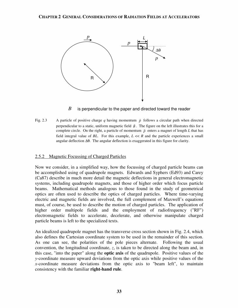
CHAPTER 2 GENERAL CONSIDERATIONS OF RADIATION FIELDS AT ACCELERATORS
33
R
pp
∆θ
L
R
p
B is perpendicular to the paper and directed toward the reader Fig. 2.3 A particle of positive charge q having momentum p
follows a circular path when directed perpendicular to a static, uniform magnetic field B
. The figure on the left illustrates this for a
complete circle. On the right, a particle of momentum p enters a magnet of length L that has
field integral value of BL. For this example, L << R and the particle experiences a small angular deflection ∆θ. The angular deflection is exaggerated in this figure for clarity.
2.5.2 Magnetic Focussing of Charged Particles Now we consider, in a simplified way, how the focussing of charged particle beams can be accomplished using of quadrupole magnets. Edwards and Syphers (Ed93) and Carey (Ca87) describe in much more detail the magnetic deflections in general electromagnetic systems, including quadrupole magnets, and those of higher order which focus particle beams. Mathematical methods analogous to those found in the study of geometrical optics are often used to describe the optics of charged particles. Where time-varying electric and magnetic fields are involved, the full complement of Maxwell’s equations must, of course, be used to describe the motion of charged particles. The application of higher order multipole fields and the employment of radiofrequency ("RF") electromagnetic fields to accelerate, decelerate, and otherwise manipulate charged particle beams is left to the specialized texts. An idealized quadrupole magnet has the transverse cross section shown in Fig. 2.4, which also defines the Cartesian coordinate system to be used in the remainder of this section. As one can see, the polarities of the pole pieces alternate. Following the usual convention, the longitudinal coordinate, z, is taken to be directed along the beam and, in this case, "into the paper" along the optic axis of the quadrupole. Positive values of the y-coordinate measure upward deviations from the optic axis while positive values of the x-coordinate measure deviations from the optic axis to "beam left", to maintain consistency with the familiar right-hand rule.
CHAPTER 2 GENERAL CONSIDERATIONS OF RADIATION FIELDS AT ACCELERATORS
34
Fig. 2.4 Cross section of a typical quadrupole magnet. The pole pieces are of opposite magnetic
polarities, denoted "N" and "S", and are of hyperbolic shapes. A Cartesian coordinate system is used in which x and y denote transverse coordinates while z is along the desired beam trajectory, the optic axis of the beam optical system. In this figure, the beam enters the quadrupole into the paper along the positive z axis. The curves with arrows denote magnetic field lines. [Adapted from (Ca87).]
Often in the accelerator magnets themselves and nearly always in beam lines transmitting extracted particles, the electromagnetic fields vary only slowly with time or are static compared with the particle transit times. Under these conditions, it is shown in other texts that if the shape of the pole pieces are hyperbolae described by equations of form xy = + k, where k is a constant, and if the pole pieces are uniformly magnetized, then the components of the magnetic field within the gap containing the beam are given by
ox
BB y gy
a= − = − , and (2.29a)
oy
BB x gx
a= − = − . (2.29b)
Here, a is the gap dimension as defined in Fig. 2.4 and Bo is the magnitude of the magnetic field strength at the pole pieces. The parameter g is, quite naturally, called the gradient of the quadrupole and in this scheme has units of Tesla meter-1. This configuration defines an ideal quadrupole, which is of length, L. Now examine qualitatively what happens to a particle having positive charge that enters this magnet parallel to the z-axis. If the particle trajectory is along the optic axis, then it
CHAPTER 2 GENERAL CONSIDERATIONS OF RADIATION FIELDS AT ACCELERATORS
35
will not be deflected at all since Bx = By = 0. If, however, the particles enter the magnet parallel to the optic axis but with some finite positive value of y, it will receive a deflection toward smaller values of y in accordance with the right hand rule and Eq. (2.25). Likewise, if it enters with a finite negative value of y, it will receive a deflection toward less negative values of y. Thus, a beam of such particles is said to be focussed in the yz plane. However, if the particle enters with a finite positive value of x, it will be deflected toward a larger value of x, away from the optic axis. Finally, a particle incident with a finite negative value of x will similarly be deflected away from the optic axis. Thus, a beam of such particles is said to be defocussed in the xz plane. From this qualitative discussion it should be evident that more than one quadrupole is needed to achieve a net focussing effect. Considering just the situation in the yz plane, it is easy to see that the analogy with geometrical optics is instructive even in mathematical detail. For a particle entering with coordinate y, one can substitute into Eq (2.28) and find that the angular deflection, if within the aperture of the magnet, is given by
0.29979qLgy
pθ∆ = (radians), (2.30)
where the same units as Eq. (2.28) have been employed, with g (Tesla meter-1) and y (meters) inserted. If the incident particle trajectory is parallel with the z-axis, the situation is schematically shown in Fig. 2.5a. It should be pointed out that in schematic drawings of beam optics, it is customary to show convex lenses to denote focussing elements and concave lenses to represent defocussing elements pertinent to a given plane. Bending magnets are correspondingly represented by prisms in such drawings. Applying simple trigonometry, one finds that after deflection in this situation, the particle trajectory will intercept the z-axis at a distance, f, given as follows:
tan 0.29979
y y pf
qLgθ θ= ≈ =
∆ ∆, (2.31)
since the deflection, θ∆ , is small. This approximation is called the thin lens approximation. In recognition of the fact that f is independent of the y coordinate, it is called the focal length of the quadrupole. By analogy with optical thin lenses, one can write down the thin lens equation which gives the relationship between the image distance, zi, and the object distance, zo, for other rays as follows:
1 1 1
o iz z f+ = . (2.32)

CHAPTER 2 GENERAL CONSIDERATIONS OF RADIATION FIELDS AT ACCELERATORS
36
a)
z-axis
yz-axis
f
∆θ
incoming trajectory
outgoingtrajectory
yz-axis
f
∆θ
incoming trajectory
outgoingtrajectory
b)
c)d
yz-axis
d
x
d)
quad 1 quad 2
quad 1 quad 2
Figure 2.5 Configurations of quadrupole lenses are shown with the symbolism explained in the text: a) Representation of focusing in the yz plane of a beam trajectory incident from the left parallel to the z-axis. A real image is formed at the focal length, f, from the lens. b) Representation of defocusing in the yz plane. The parallel beam is deflected so that it appears to emerge from a point a distance f before the lens, thus, forming a virtual image. c) Representation of a particle trajectory in the yz plane of a quadrupole doublet. The particle enters a quadrupole doublet parallel to the z-axis from the left. First a focusing quadrupole (quad 1) is encountered and then a defocussing quadrupole (quad 2) follows. d) Representation of a particle trajectory in the xz plane of the same doublet. The particle enters the doublet parallel to the z-axis. In this plane, the defocussing quadrupole is encountered first.
CHAPTER 2 GENERAL CONSIDERATIONS OF RADIATION FIELDS AT ACCELERATORS
37
In this equation, zo and zi are > 0 if the object is to the left of the lens and the image is to the right of the lens, forming a real image, for a focussing lens with f > 0. The situation for the defocussing plane, here the xz plane, is shown in Fig. 2.5b as a concave lens. For that plane, the equations are still workable if one applies a negative sign to the value of f and understands that a value of zi < 0 describes a virtual image. The simplest configuration of quadrupole magnets is in the form of a pair of two such magnets. In a given plane, say the yz, the first would be focussing while the second would be defocussing. In the orthogonal plane, here the xz, the defocussing quadrupole would thus be encountered first. Generally, these magnets will be of identical dimensions and have gradients of similar magnitudes. Such a quadrupole doublet is shown in Figs 2.5c and 2.5d for the yz and xz planes, respectively. Eq. (2.32) can now be employed to explore how a quadrupole doublet can focus a parallel beam in both the xz and yz planes in a simple example. For the sake of this discussion, the quadrupoles, quad 1 and quad 2, have different focal lengths, f1 and f2, respectively, and are separated by distance d. Quad 1 is focussing in the yz plane. As one would do in geometrical optics, for an incoming parallel beam, the object distance relative to quad 1 is zyo1 → ∞ . Thus, the image distance from quad 1 is at zyi1 = f1. The object distance of this image from quad 2 is thus zyo2 = d - f1. Relative to quad 2, the location of the final image will be at zyi2 by means of the thin lens equation;
2 2 1
1 1 1
yiz f d f= −
− −, (2.33)
where the negative coefficient of f2 explicitly incorporates the fact that lens 2 is defocussing in the yz plane. Solving,
2 12
2 1
( )yi
f f dz
f f d−=
− +. (2.34a)
If the quadrupoles are identical (f = f1 = f2), then,
2( )
yif f d
zd
−= . (2.34b)
It is simple to follow the same procedure for the xz plane to obtain the corresponding image distance, zxi2,
2 1
21 2
( )xi
f f dz
f f d+=
− +. (2.35a)
CHAPTER 2 GENERAL CONSIDERATIONS OF RADIATION FIELDS AT ACCELERATORS
38
With identical quadrupoles, this becomes
2( )
xif f d
zd
+= . (2.35b)
One should notice that with identical quadrupoles, 2 2 2xi yiz z f− = , (2.36)
a result that should not be surprising given that particles in xz plane are first subject to defocussing, and thus become more divergent, prior to their being focussed. The average
focal length of the system for both the xz and yz planes is thus 2 /f d . More sophisticated schemes such as quadrupole triplets and non-identical magnets can be used, where needed, to obtain a specialized beam envelope. These advanced methods are discussed in great detail, for example, by Carey (Ca87). In this simple exposition, a number of significant effects have been ignored. First, a typical particle beam will contain some spread in particle momenta. The derivation given above ignores the fact that dispersion will occur in the magnetic fields in the same way that prism disperses a visible beam of "white" light into the various colors. There also may be aberrations or distortions of an image. One such aberration is called chromatic aberration, analogous to its namesake encountered in geometrical optics. For particle beams chromatic aberration is due to the dependence of focal length on particle momentum evident from Eq. (2.31). Also, the fact that no particle beam is ever completely parallel or completely emergent from a geometrical point has also been ignored. All particle beams possess a property called transverse emittance. This quantity is expressed in units of angular divergence times physical size, typically in units of π mm-mradian. The explicit display of the factor π is a matter of custom. The emittance concept is used to describe both longitudinal and transverse phenomena and is discussed by Carey (Ca87) and by Edwards and Syphers (Ed93). The discussion here is limited to transverse emittance. During the process of accelerating particles, the beam emittance in general becomes smaller because the normalized transverse emittance [the emittance when multiplied by the relativistic factors from Eqs. (1.10) and (1.11)] is an invariant. Thus, as velocity increases, the unnormalized emittance must decrease since the product γβ increases with particle momentum. There are exceptions to this generalization beyond the scope of this discussion. Once a beam is no longer subject to accelerating electromagnetic fields (e.g. by RF waves) in an accelerator, the emittance can generally no longer be made smaller and can only increase due to processes such as multiple Coulomb scattering, space charge effects, etc.6 Under conditions in which the emittance
6 Under some conditions not discussed further in this text, synchrotron radiation can, in fact, reduce the transverse emittance.
CHAPTER 2 GENERAL CONSIDERATIONS OF RADIATION FIELDS AT ACCELERATORS
39
is constant, the product of the angular divergence of the beam envelope and the transverse size of the beam envelope is conserved.7 This means that efforts made to focus the beam tightly into a smaller cross-sectional size will unavoidably result in a beam with a correspondingly larger angular spread. Likewise, attempts to create a parallel beam (one with essentially no angular spread) will result in a correspondingly larger beam size. As a final word, one should be aware of the fact that the above discussion of quadrupoles depends upon the beam axis coinciding with the optic axis. Should the beam enter a quadrupole with its center far off-axis, it should be obvious that the entire beam will be deflected nearly as if a quadrupole were a dipole magnet of equivalent field strength and length (see Fig. 2.4). Beams that are deflected in this manner by a quadrupole are said to have suffered steering. The steering of beams can constitute significant loss points in the beam transport system.
7 This is a consequence of Liouville’s theorem of classical dynamics as applied to the coordinate system defined here which requires that the volume of the phase space defined by the transverse spatial coordinates; x and y, and their corresponding “conjugate” momentum components, px and py; is conserved. Since in this Cartesian coordinate system, the momentum components px and py are, in small angle approximation, directly proportional to the angles (in radians) between the momentum vector and the x and y coordinate axes, respectively, the assertion made above directly follows. Other texts address this point in more detail (e.g., Ca87).

CHAPTER 2 GENERAL CONSIDERATIONS OF RADIATION FIELDS AT ACCELERATORS
40
Problems 1. This problem gives two elementary examples of Monte Carlo techniques that are
almost "trivial". In this problem, obtaining random numbers from a standard table or from a hand calculator should be helpful.
a) First, use a random number table or random number function on a calculator
along with the facts given about the cumulative probability distribution for exponential attenuation to demonstrate that, even for a sample size as small as, say, 15, the mean value of paths traveled is "within expectations" if random numbers are used to select those path lengths from the cumulative distribution. Do this, for example, by calculating the mean and standard deviation of your distribution.
b) An incident beam is subjected to a position measurement in the coordinate x. It is
desirable to "recreate" incident beam particles for a shielding study using Monte Carlo. The x distribution as measured is as follows:
x # 0 0 1 1 2 2 3 3 4 4 5 5 6 4 7 3 8 2 9 1 10 0
Determine, crudely, p(x), P(x) and then use 50 random numbers to "create"
particles intended to represent this distribution. Then compare with the original one which was measured in terms of the average value of x and its standard deviation. Do not take the time to use interpolated values of x, simply round off to integer values of x for this demonstration.
2. A beam of protons having a kinetic energy of 100 GeV is traveling down a beam
line. The beam is entirely contained within a circle of diameter 1 cm. All of the beam particles have the same kinetic energy. An enclosure further downstream must be protected from the beam or secondary particles produced by the beam by shielding it with a large diameter iron block that is 20 cm in radius centered on the beam line. The beam passes by this block by being deflected by a uniform field magnet that is 3 meters long, the longitudinal center of which is located 30 meters upstream of the iron block. Calculate the magnetic field, B, that is needed to accomplish this objective.
CHAPTER 3 PROMPT RADIATION FIELDS DUE TO ELECTRONS
41
3.1 Introduction In this chapter the major features of the prompt radiation fields produced by electrons are described. An extensive discussion of the electromagnetic cascade and of the shielding of photoneutrons and high energy particles that result from these interactions is given. The utilization of Monte Carlo calculations in electron shielding problems is also addressed. The material presented in this chapter is useful for understanding electron, photon, and photoneutron radiation from electron accelerators used in medicine and in high energy physics research. As has been pointed out by Silari et al. (Si99), some of the content discussed in this chapter is also useful in understanding the radiation that may be produced by certain accelerator components, such as RF cavities (including superconducting ones), even when operated apart from the main accelerator. 3.2 Unshielded Radiation Produced by Electron Beams At all energies photons produced by bremsstrahlung dominate the unshielded radiation field aside from the hazard of the direct beam. As the energy increases, neutrons become a significant problem. For electrons having kinetic energy Eo approaching 100 MeV, the electromagnetic cascade is of great importance. A useful rule of thumb is that electrons have a finite ionization range, R, in any material that monotonically increases with the initial kinetic energy, Eo, (MeV). For 2 < Eo < 10 MeV,
R = 0.6Eo (g cm-2). (3.1) In air at standard temperature and pressure (STP) over this energy domain, R (meters) ≈ 5 Eo (MeV). Above an energy of 10 MeV or so, a threshold that we will see is dependent upon the absorbing medium, the loss of energy begins to be dominated by radiative processes, whereby photons that are emitted begin to dominate over those losses of energy due to collisions. This transition will be discussed further in Section 3.2.2. 3.2.1 Dose Equivalent Rate in a Direct Beam of Electrons At any accelerator, the dose equivalent rate in the direct particle beam is generally larger than in any purely secondary radiation field. This is certainly true at electron accelerators. Swanson (Sw79a) has given a rule of thumb, said to be “conservative”, for electrons in the energy domain of 1 < Eo < 100 MeV;
dHdt
= × −16 10 4. φ , (3.2)
where dH/dt is the dose equivalent rate (rem h-1) and φ is the flux density (cm-2 s-1) in the electron beam. One of the problems at the end of this chapter examines the domain of validity of this approximation. The coefficient is 1.6 x 10⁻⁶ if dH/dt is to be in Sv h-1 with φ remaining in units of cm-2 s-1.
CHAPTER 3 PROMPT RADIATION FIELDS DUE TO ELECTRONS
42
3.2.2 Bremsstrahlung Bremsstrahlung is the radiative energy loss of charged particles, especially electrons, as they interact with materials. It appears in the form of photons. An important parameter when considering the radiative energy loss of electrons in matter is the critical energy, Ec. The critical energy is the energy above which the radiative loss of energy exceeds that due to ionization. There are several formulae used to calculate Ec, representative ones are given here. For electrons, the value of Ec is a smooth function of atomic number, approximated by
800 (MeV)
1.2cEZ
=+
, (3.3a)
where Z is the atomic number of the material. For muons in solid materials (see Section 1.4.1) the corresponding critical energy, Ec,muon, is much larger and differs for solid and gaseous media (PDG04);
( ), 0.838
5700 GeV
Z + 1.47c muonE = (solids), and
( ), 0.879
7980 GeV
Z + 2.03c muonE = (gases). (3.3b)
The transition from dominance by ionization to dominance by radiation is a smooth one. The total stopping power for electrons or muons may be written as the sum of collisional and radiative components, respectively;
dEdx
dEdx
dEdxtot coll rad
=
+
. (3.4)
Another parameter of significant importance is the radiation length, Xo, which is the mean thickness of material over which a high energy electron loses all but 1/e of its energy by bremsstrahlung. This parameter is the approximate scale length for describing high energy electromagnetic cascades, supplanting the ionization range for even moderate electron energies. It also plays a role in the "scaling" of multiple Coulomb scattering for all charged particles and was discussed in that context in Section 1.4.2. The radiation length is approximated by Eq. (1.21). For energetic electrons, the fractional energy loss is equal to the fraction of a radiation length it penetrates;
0 0
dE, thus
dxrad
rad
dE dx EE X X
= − = −
, (3.5)
so that under these conditions (i.e., where loss by ionization can be neglected), the energy of the electron, E, as a function of thickness of shield penetrated, x, is given by ( ) exp( / )o oE x E x X= − , (3.6) where the energy of the incident particle is Eo and x and Xo are in the same units.
CHAPTER 3 PROMPT RADIATION FIELDS DUE TO ELECTRONS
43
0
20
40
60
80
100
0 20 40 60 80 100
Rad
iatio
n Y
ield
(%)
Eo (MeV)
Pb
NaI
Cu
AlH
2O
C
He
H
Fig. 3.1 Bremsstrahlung efficiency for electrons stopped in various materials. This is the fraction (in
per cent) of the kinetic energy of incident electrons converted to radiation as a function of incident energy Eo. The remainder of the kinetic energy is transferred to the medium by ionization. [Adapted from (Sw79a).]
Figure 3.1 gives the percentage of energy Eo that appears as radiation for various materials as a function of energy. External bremsstrahlung develops as a function of target thickness and is described by a transition curve. As the thickness increases, the intensity of the radiation increases until re-absorption begins to take effect. Then, self-shielding begins to take over. One talks about conditions at the maximum as being a "thick-target" bremsstrahlung spectrum. This phenomenon becomes dominant above energies of about 100 MeV for low atomic number (“low-Z”) materials and above 10 MeV for high atomic number (“high-Z”) materials. The energy spectrum of the radiated photons ranges from zero to the energy of the incident electron and the number of photons in a given energy interval is approximately inversely proportional to the photon energy. The amount of energy radiated per energy interval is practically constant according to Schopper et al. (Sc90). Detailed spectral information for bremsstrahlung photons has been provided by various workers. Figures 3.2 and 3.3 are provided as examples of such spectra at moderate electron beam energies. Bremsstrahlung spectra are noticeably more energetic (i.e., “harder”) at forward angles.
CHAPTER 3 PROMPT RADIATION FIELDS DUE TO ELECTRONS
44
For thin targets of thickness x (x << Xo), the spectrum of photons of energy k per energy interval dk, dN/dk, can be approximated by
o
dN xdk X k
≈ . (3.7)
Thick targets may require consideration of the electromagnetic cascade. In general, the spectra fall as 1/k 2 at θ = 0 and even faster at larger angles (Sw79a). A more detailed parameterization of the normalized total photon differential yield per incident electron, dN/dΩ, for photons of all energies has been reported by Swanson and Thomas (Sw90), with improvements suggested by Nelson (Ne97);
0.614.76 exp( ) 1.08exp( / 72)o
o
dNE
E dθ θ= − + −
Ω (photons sr-1 GeV-1 electron-1). (3.8)
This expression is normalized to results involving iron and copper targets of thicknesses of about 17 Xo at Eo = 15 GeV. In Eq. (3.8), Eo is in GeV and θ is in degrees. As will be shown below, this formalism is especially useful as a source term in thick shields and is particular valid for scattering angles around 90 degrees.
Fig. 3.2 Bremsstrahlung spectra measured at zero degrees from intermediate thickness (0.2 Xo) targets
of high atomic number (Z) material. The data points are measurements of O'Dell et al. (OD68) [adapted by Swanson (Sw79a)].
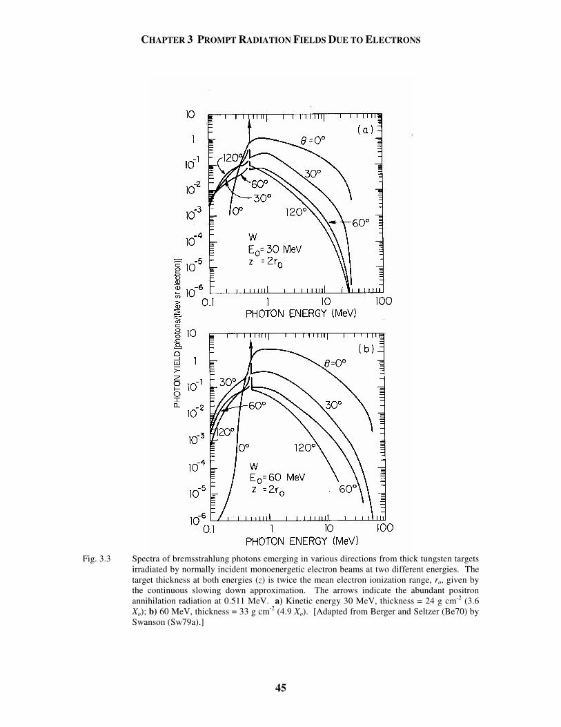
CHAPTER 3 PROMPT RADIATION FIELDS DUE TO ELECTRONS
45
Fig. 3.3 Spectra of bremsstrahlung photons emerging in various directions from thick tungsten targets
irradiated by normally incident monoenergetic electron beams at two different energies. The target thickness at both energies (z) is twice the mean electron ionization range, ro, given by the continuous slowing down approximation. The arrows indicate the abundant positron annihilation radiation at 0.511 MeV. a) Kinetic energy 30 MeV, thickness = 24 g cm-2 (3.6 Xo); b) 60 MeV, thickness = 33 g cm-2 (4.9 Xo). [Adapted from Berger and Seltzer (Be70) by Swanson (Sw79a).]
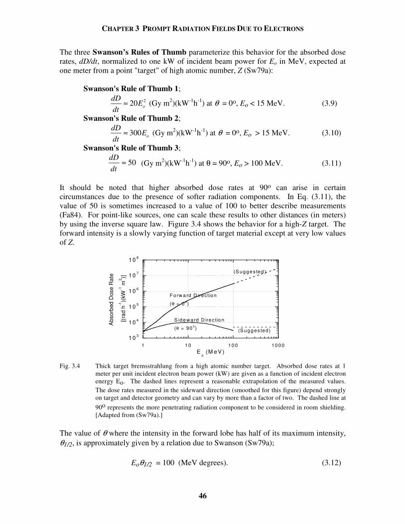
CHAPTER 3 PROMPT RADIATION FIELDS DUE TO ELECTRONS
46
The three Swanson’s Rules of Thumb parameterize this behavior for the absorbed dose rates, dD/dt, normalized to one kW of incident beam power for Eo in MeV, expected at one meter from a point "target" of high atomic number, Z (Sw79a): Swanson's Rule of Thumb 1;
220 o
dDE
dt≈
(Gy m2)(kW-1h-1) at θ = 0o, Eo < 15 MeV. (3.9)
Swanson's Rule of Thumb 2;
300 o
dDE
dt≈ (Gy m2)(kW-1h-1) at θ = 0o, Eo > 15 MeV. (3.10)
Swanson's Rule of Thumb 3;
dDdt
≈ 50 (Gy m2)(kW-1h-1) at θ = 90o, Eo > 100 MeV. (3.11)
It should be noted that higher absorbed dose rates at 90o can arise in certain circumstances due to the presence of softer radiation components. In Eq. (3.11), the value of 50 is sometimes increased to a value of 100 to better describe measurements (Fa84). For point-like sources, one can scale these results to other distances (in meters) by using the inverse square law. Figure 3.4 shows the behavior for a high-Z target. The forward intensity is a slowly varying function of target material except at very low values of Z.
1 0 3
1 0 4
1 0 5
1 0 6
1 0 7
1 0 8
1 1 0 10 0 10 0 0
Abs
orbe
d D
ose
Rat
e
[(rad
h-1
)(kW
-1 m
2 )]
Eo (M e V )
F o rw a rd D irec tion
(θ = 0 o)
S ide w a rd D ire ctio n
(θ = 90 o)
(S ugge s ted )
(S ugges ted )
Fig. 3.4 Thick target bremsstrahlung from a high atomic number target. Absorbed dose rates at 1
meter per unit incident electron beam power (kW) are given as a function of incident electron energy Eo. The dashed lines represent a reasonable extrapolation of the measured values. The dose rates measured in the sideward direction (smoothed for this figure) depend strongly on target and detector geometry and can vary by more than a factor of two. The dashed line at 90o represents the more penetrating radiation component to be considered in room shielding. [Adapted from (Sw79a).]
The value of θ where the intensity in the forward lobe has half of its maximum intensity, θ1/2, is approximately given by a relation due to Swanson (Sw79a); Eoθ1/2 = 100 (MeV degrees). (3.12)
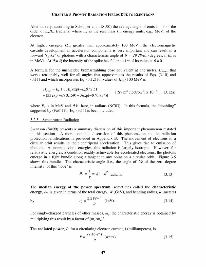
CHAPTER 3 PROMPT RADIATION FIELDS DUE TO ELECTRONS
47
Alternatively, according to Schopper et al. (Sc90) the average angle of emission is of the order of me/Eo (radians) where me is the rest mass (in energy units, e.g., MeV) of the electron. At higher energies (Eo greater than approximately 100 MeV), the electromagnetic cascade development in accelerator components is very important and can result in a forward "spike" of photons with a characteristic angle of θc = 29.28/Eo (degrees, if Eo is in MeV). At θ = θc the intensity of the spike has fallen to 1/e of its value at θ = 0. A formula for the unshielded bremsstrahlung dose equivalent at one meter, Hbrem, that works reasonably well for all angles that approximates the results of Eqs. (3.10) and (3.11) and which incorporates Eq. (3.12) for values of E0 > 100 MeV is
0 0 0[1.33 exp( / 2.51)
133exp( / 0.159) 3exp( / 0.834)]bremH E E E θ
θ θ= −
+ − + − [(Sv m2 electron-1) x 10-17], (3.12a)
where Eo is in MeV and θ is, here, in radians (NC03). In this formula, the “doubling” suggested by (Fa84) for Eq. (3.11) is been included. 3.2.3 Synchrotron Radiation Swanson (Sw90) presents a summary discussion of this important phenomenon restated in this section. A more complete discussion of this phenomenon and its radiation protection ramifications is provided in Appendix B. The movement of electrons in a circular orbit results in their centripetal acceleration. This gives rise to emission of photons. At nonrelativistic energies, this radiation is largely isotropic. However, for relativistic energies, a condition readily achievable for accelerated electrons, the photons emerge in a tight bundle along a tangent to any point on a circular orbit. Figure 3.5 shows this bundle. The characteristic angle (i.e., the angle of 1/e of the zero degree intensity) of this "lobe" is
θγ
βc = = −1
1 2radians. (3.13)
The median energy of the power spectrum, sometimes called the characteristic energy, εc, is given in terms of the total energy, W (GeV), and bending radius, R (meters)
by 32.218
c
WR
ε = (keV). (3.14)
For singly-charged particles of other masses, mx, the characteristic energy is obtained by multiplying this result by a factor of (me /mx)3. The radiated power, P, for a circulating electron current, I (milliamperes), is
488.46W IP
R= (watts). (3.15)
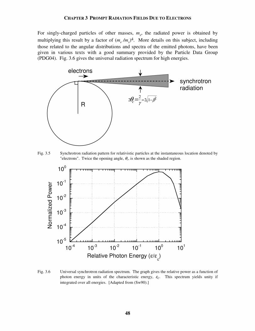
CHAPTER 3 PROMPT RADIATION FIELDS DUE TO ELECTRONS
48
For singly-charged particles of other masses, mx, the radiated power is obtained by multiplying this result by a factor of (me /mx)4. More details on this subject, including those related to the angular distributions and spectra of the emitted photons, have been given in various texts with a good summary provided by the Particle Data Group (PDG04). Fig. 3.6 gives the universal radiation spectrum for high energies.
R
electrons
22
2 1 2θ γ βc = = −
synchrotronradiation
Fig. 3.5 Synchrotron radiation pattern for relativistic particles at the instantaneous location denoted by
"electrons". Twice the opening angle, θc, is shown as the shaded region.
10-5
10-4
10-3
10-2
10-1
100
10-4 10-3 10-2 10-1 100 101
Nor
mal
ized
Pow
er
Relative Photon Energy (ε/εc)
Fig. 3.6 Universal synchrotron radiation spectrum. The graph gives the relative power as a function of
photon energy in units of the characteristic energy, εc. This spectrum yields unity if integrated over all energies. [Adapted from (Sw90).]
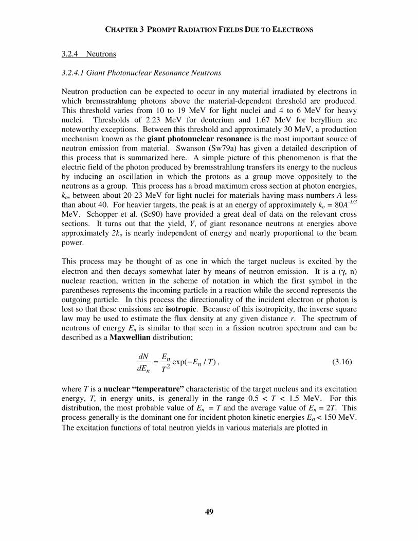
CHAPTER 3 PROMPT RADIATION FIELDS DUE TO ELECTRONS
49
3.2.4 Neutrons 3.2.4.1 Giant Photonuclear Resonance Neutrons Neutron production can be expected to occur in any material irradiated by electrons in which bremsstrahlung photons above the material-dependent threshold are produced. This threshold varies from 10 to 19 MeV for light nuclei and 4 to 6 MeV for heavy nuclei. Thresholds of 2.23 MeV for deuterium and 1.67 MeV for beryllium are noteworthy exceptions. Between this threshold and approximately 30 MeV, a production mechanism known as the giant photonuclear resonance is the most important source of neutron emission from material. Swanson (Sw79a) has given a detailed description of this process that is summarized here. A simple picture of this phenomenon is that the electric field of the photon produced by bremsstrahlung transfers its energy to the nucleus by inducing an oscillation in which the protons as a group move oppositely to the neutrons as a group. This process has a broad maximum cross section at photon energies, ko, between about 20-23 MeV for light nuclei for materials having mass numbers A less than about 40. For heavier targets, the peak is at an energy of approximately ko = 80A-1/3 MeV. Schopper et al. (Sc90) have provided a great deal of data on the relevant cross sections. It turns out that the yield, Y, of giant resonance neutrons at energies above approximately 2ko is nearly independent of energy and nearly proportional to the beam power. This process may be thought of as one in which the target nucleus is excited by the electron and then decays somewhat later by means of neutron emission. It is a (γ, n) nuclear reaction, written in the scheme of notation in which the first symbol in the parentheses represents the incoming particle in a reaction while the second represents the outgoing particle. In this process the directionality of the incident electron or photon is lost so that these emissions are isotropic. Because of this isotropicity, the inverse square law may be used to estimate the flux density at any given distance r. The spectrum of neutrons of energy En is similar to that seen in a fission neutron spectrum and can be described as a Maxwellian distribution;
dNdE
E
TE T
n
nn= −2 exp( / ) , (3.16)
where T is a nuclear “temperature” characteristic of the target nucleus and its excitation energy, T, in energy units, is generally in the range 0.5 < T < 1.5 MeV. For this distribution, the most probable value of En = T and the average value of En = 2T. This process generally is the dominant one for incident photon kinetic energies Eo < 150 MeV. The excitation functions of total neutron yields in various materials are plotted in

CHAPTER 3 PROMPT RADIATION FIELDS DUE TO ELECTRONS
50
Fig. 3.7. Table 3.1 gives the high energy limits for total yield, Yn, of giant resonance neutrons per watt of beam power (s-1W-1), the isotropic differential neutron yield, dYn/dΩ (GeV-1 sr-1) per unit of beam energy per electron, and a recommended dose equivalent source term, Sn, (Sv cm2 GeV-1) per unit beam energy per electron to be used as follows:
HS
rE In= 2 0 , (3.17)
where H is the dose equivalent in Sieverts, r is the radial distance from the target in cm, Eo is in GeV, and I is the total number of beam particles incident (e.g., during some time interval). For electron energies below 500 MeV, appropriate values can be obtained by scaling the Table 3.1 entries according to the Fig. 3.7 curves. The agreement with various experiments is quite good according to Schopper et al. (Sc90). The use of these “saturation” values can support reasonable, but conservative, estimates.
1 1 0 1 0 00
1
2
3
4
Y (n
eutr
ons
s-1 k
w-1
) x10
12
Eo ( M e V )
C
A lF e
C u
A g
P bW
U
Fig. 3.7 Neutron yields from infinitely thick targets per kW of electron beam power as a function of
electron beam energy Eo, ignoring target self-shielding. [Adapted from (Sw79b).]
CHAPTER 3 PROMPT RADIATION FIELDS DUE TO ELECTRONS
51
Table 3.1 Total neutron yield rate per unit beam power (s-1 watt-1), differential yield per unit electron energy (GeV-1 sr-1) per electron, and source term per unit electron energy (Sv cm2 GeV-1) per electron for giant resonance neutrons in an optimum target. No energy dependence "near threshold" is assumed. The neutrons are distributed uniformly over all directions (4ππππ steradians). These results are best used for Eo > 0.5 GeV. [Adapted from (Sw79b) and (Sc90).]
Material Total Neutron Production
Yn (s-1W-1)
Differential Neutron Yield
dYn/dΩΩΩΩ (GeV-1sr-1) per electron
Recommended Source Terms a, Sn
(Sv cm2 GeV-1) per electron C 4.4 x 10⁸ 5.61 x 10⁻³ 4.3 x 10⁻¹²
Alb 6.2 x 10⁸ 7.90 x 10⁻³ 6.0 x 10⁻¹² Fe 8.18 x 10⁸ 1.04 x 10⁻² 7.7 x 10⁻¹² Ni 7.36 x 10⁸ 9.38 x 10⁻³ 6.9 x 10⁻¹² Cu 1.18 x 10⁹ 1.50 x 10⁻² 1.1 x 10⁻¹¹ Ag 1.68 x 10⁹ 2.14 x 10⁻² 1.5 x 10⁻¹¹ Ba 1.94 x 10⁹ 2.47 x 10⁻² 1.8 x 10⁻¹¹ Ta 2.08 x 10⁹ 2.65 x 10⁻² 1.8 x 10⁻¹¹ W 2.36 x 10⁹ 3.01 x 10⁻² 2.0 x 10⁻¹¹ Au 2.02 x 10⁹ 2.58 x 10⁻² 1.8 x 10⁻¹¹ Pb 2.14 x 10⁹ 2.73 x 10⁻² 1.9 x 10⁻¹¹ U 3.48 x 10⁹ 4.44 x 10⁻² 3.0 x 10⁻¹¹
aTo get Sv cm2 h-1kW-1, multiply this column by 2.25 x 10¹⁶. bThe value for aluminum is also recommended for concrete. 3.2.4.2 Quasi-Deuteron Neutrons At energies above the giant resonance, the dominant neutron production mechanism is one in which the photon interacts with a neutron-proton pair within the nucleus rather than with the whole nucleus. The quasi-deuteron effect is so-named because for Eo ≈ 30 MeV the photon wavelength is near resonance with the average inter-nucleon distance so that the photon interactions tend to occur with "pairs" of nucleons. Only neutron-proton pairs have a nonzero electric dipole moment, which makes interactions of photons with such pairs (pseudo-deuterons) favorable. This mechanism is important for 30 < Eo < 300 MeV and has been described by Swanson (Sw79b). An important general effect due to this mechanism is to add a tail of higher-energy neutrons to the giant resonance spectrum. For 5 < En < Eo/2 (MeV), the nearly isotropic spectrum of quasi-deuteron neutrons is given by
α−= nn
EdEdN
where, approximately, 1.7 < α < 3.6. (3.18)
The slope becomes steeper as Eo, the kinetic energy of the incident electron, is approached. Eq. (3.18) is for thin targets. For thick target situations, the fall-off with En is generally steeper. Since the mechanism is the (γ, np) reaction and the neutron and the proton are nearly identical in mass, they share the available energy equally so that the yield of neutrons due this mechanism is essentially zero for neutrons having kinetic
CHAPTER 3 PROMPT RADIATION FIELDS DUE TO ELECTRONS
52
energy En > Eo/2. In general, the quasi-deuteron neutrons are fewer in number and generally less important than are the giant resonance neutrons. Shielding against the latter will usually provide adequate protection against the former for shielding purposes, but should not be neglected for questions where the fluences of particularly energetic neutrons may be important. 3.2.4.3 Neutrons Associated with the Production of Other Particles There are interactions in which the production of other elementary particles, perhaps best typified by pions, becomes energetically possible at still higher energies (say, Eo > 300 MeV). These particles can then produce neutrons through secondary interactions as will be discussed in Chapter 4. The neutrons from this source tend to dominate the lateral shielding requirements in the GeV region. DeStaebler (De65) has parameterized the measured yields of high energy particles per incident electron;
2 4
-1 -12 0.4
7.5 10 (GeV sr )
(1 0.75cos )nd Y
dEd Aθ
−×=Ω −
, (3.19)
where A is the atomic mass (g mole-1) of the target material. It is reasonable to use a dose equivalent per fluence conversion factor of approximately 1 x 10-13 Sv m2 (10-3 µSv cm2) for these neutrons (see Fig. 1.5). Obviously, these neutrons are forward-peaked, not isotropically distributed. In general photons are produced more copiously, but the neutrons can be more difficult to shield. 3.2.5 Muons With electron beams, muons become of significance above an electron energy of approximately 211 MeV, the threshold of the process in which a µ+ pair is produced in a pair production process quite analogous to the more familiar one in which an electron-positron pair results from photon interactions. They can be produced, with much smaller yields, at electron accelerators by the decay of π+ and K+ which are, in turn, due to secondary production processes exemplified by photo-pion creation. Such decay muons, which are more prominent at hadron accelerators, will be discussed in Section 4.2.4. A detailed theoretical treatment of muon production by incident electrons is given by Nelson (Ne68 and Ne74). Figure 3.8 gives the muon flux density as a function of electron energy at θ = 0o
while Fig. 3.9 shows an example of the angular dependence of these yields at Eo = 20 GeV. The reasonableness of scaling with energy to larger values of Eo is well demonstrated. Obviously, the range-energy relation of muons and considerations related to their energy loss mechanisms discussed in Section 1.4.1 is relevant to shielding against muons regardless of their origin.
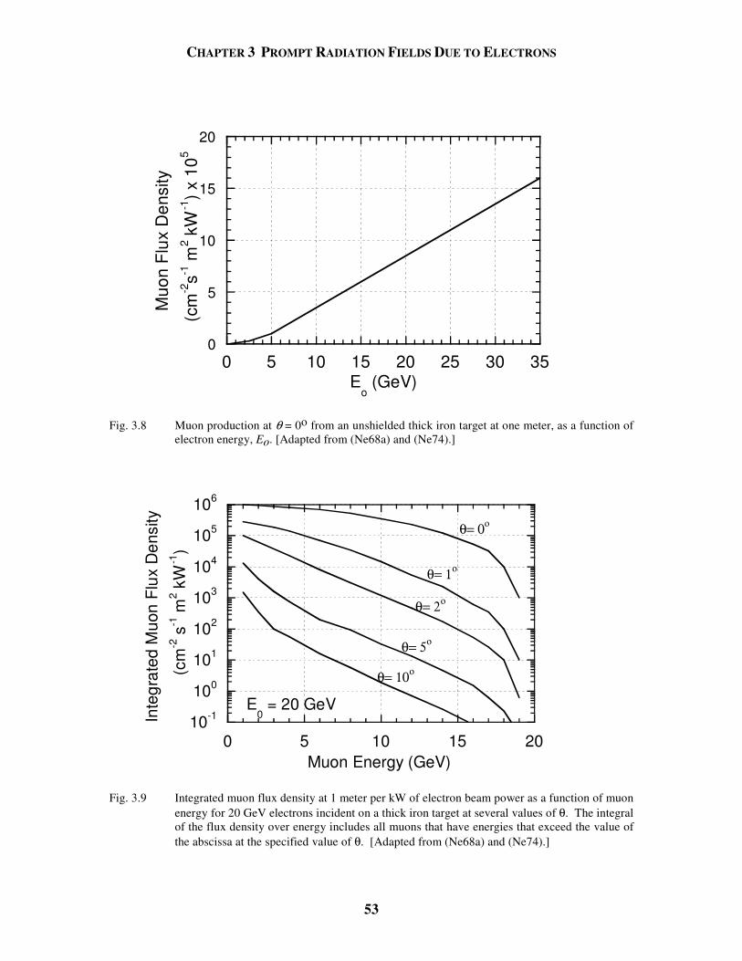
CHAPTER 3 PROMPT RADIATION FIELDS DUE TO ELECTRONS
53
0
5
10
15
20
0 5 10 15 20 25 30 35
Muo
n F
lux
Den
sity
(cm
-2s-1
m2 k
W-1
) x 1
05
Eo (GeV)
Fig. 3.8 Muon production at θ = 0o from an unshielded thick iron target at one meter, as a function of
electron energy, Eo. [Adapted from (Ne68a) and (Ne74).]
10-1
100
101
102
103
104
105
106
0 5 10 15 20
Inte
grat
ed M
uon
Flux
Den
sity
(cm
-2 s
-1 m
2 kW
-1)
Muon Energy (GeV)
θ= 0ο
θ= 1ο
θ= 2ο
θ= 5ο
θ= 10ο
E0 = 20 GeV
Fig. 3.9 Integrated muon flux density at 1 meter per kW of electron beam power as a function of muon
energy for 20 GeV electrons incident on a thick iron target at several values of θ. The integral of the flux density over energy includes all muons that have energies that exceed the value of the abscissa at the specified value of θ. [Adapted from (Ne68a) and (Ne74).]
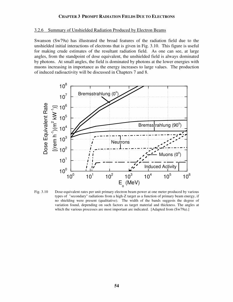
CHAPTER 3 PROMPT RADIATION FIELDS DUE TO ELECTRONS
54
3.2.6 Summary of Unshielded Radiation Produced by Electron Beams Swanson (Sw79a) has illustrated the broad features of the radiation field due to the unshielded initial interactions of electrons that is given in Fig. 3.10. This figure is useful for making crude estimates of the resultant radiation field. As one can see, at large angles, from the standpoint of dose equivalent, the unshielded field is always dominated by photons. At small angles, the field is dominated by photons at the lower energies with muons increasing in importance as the energy increases to large values. The production of induced radioactivity will be discussed in Chapters 7 and 8.
100
101
102
103
104
105
106
107
108
100 101 102 103 104 105 106
Dos
e E
quiv
alen
t Rat
e
[(rem
h-1
)(m
2 kW
-1)]
Eo (MeV)
Bremsstrahlung (0o)
Bremsstrahlung (90o)
Neutrons
Induced Activity
Muons (0o)
Fig. 3.10 Dose-equivalent rates per unit primary electron beam power at one meter produced by various
types of "secondary" radiations from a high-Z target as a function of primary beam energy, if no shielding were present (qualitative). The width of the bands suggests the degree of variation found, depending on such factors as target material and thickness. The angles at which the various processes are most important are indicated. [Adapted from (Sw79a).]
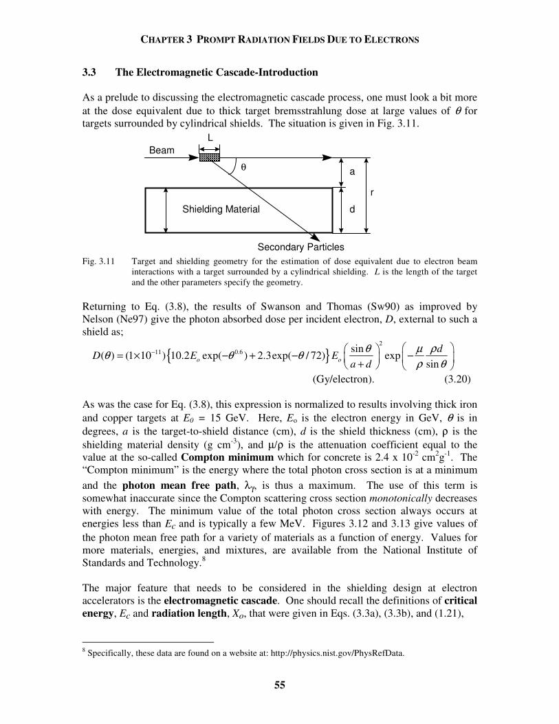
CHAPTER 3 PROMPT RADIATION FIELDS DUE TO ELECTRONS
55
3.3 The Electromagnetic Cascade-Introduction As a prelude to discussing the electromagnetic cascade process, one must look a bit more at the dose equivalent due to thick target bremsstrahlung dose at large values of θ for targets surrounded by cylindrical shields. The situation is given in Fig. 3.11.
LBeam
a
d
θ
r
Secondary Particles
Shielding Material
Fig. 3.11 Target and shielding geometry for the estimation of dose equivalent due to electron beam
interactions with a target surrounded by a cylindrical shielding. L is the length of the target and the other parameters specify the geometry.
Returning to Eq. (3.8), the results of Swanson and Thomas (Sw90) as improved by Nelson (Ne97) give the photon absorbed dose per incident electron, D, external to such a shield as;
2
11 0.6 sin( ) (1 10 ) 10.2 exp( ) 2.3exp( / 72) exp
sino o
dD E E
a dθ µ ρθ θ θ
ρ θ− = × − + − − +
(Gy/electron). (3.20)
As was the case for Eq. (3.8), this expression is normalized to results involving thick iron and copper targets at E0 = 15 GeV. Here, Eo is the electron energy in GeV, θ is in degrees, a is the target-to-shield distance (cm), d is the shield thickness (cm), ρ is the shielding material density (g cm-3), and µ/ρ is the attenuation coefficient equal to the value at the so-called Compton minimum which for concrete is 2.4 x 10⁻² cm2g-1. The “Compton minimum” is the energy where the total photon cross section is at a minimum and the photon mean free path, λγ, is thus a maximum. The use of this term is somewhat inaccurate since the Compton scattering cross section monotonically decreases with energy. The minimum value of the total photon cross section always occurs at energies less than Ec and is typically a few MeV. Figures 3.12 and 3.13 give values of the photon mean free path for a variety of materials as a function of energy. Values for more materials, energies, and mixtures, are available from the National Institute of Standards and Technology.8
The major feature that needs to be considered in the shielding design at electron accelerators is the electromagnetic cascade. One should recall the definitions of critical energy, Ec and radiation length, Xo, that were given in Eqs. (3.3a), (3.3b), and (1.21),
8 Specifically, these data are found on a website at: http://physics.nist.gov/PhysRefData.
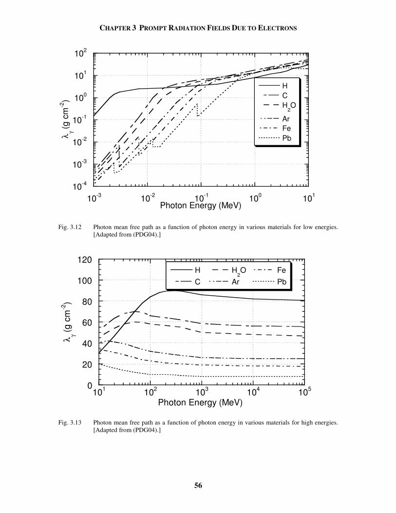
CHAPTER 3 PROMPT RADIATION FIELDS DUE TO ELECTRONS
56
10-4
10-3
10-2
10-1
100
101
102
10-3 10-2 10-1 100 101
HCH
2O
ArFePbλ γ (g
cm
-2)
Photon Energy (MeV)
Fig. 3.12 Photon mean free path as a function of photon energy in various materials for low energies.
[Adapted from (PDG04).]
0
20
40
60
80
100
120
101 102 103 104 105
HC
H2O
ArFePb
λ γ (g c
m-2
)
Photon Energy (MeV)
Fig. 3.13 Photon mean free path as a function of photon energy in various materials for high energies. [Adapted from (PDG04).]
CHAPTER 3 PROMPT RADIATION FIELDS DUE TO ELECTRONS
57
respectively. A related parameter of importance for describing the electromagnetic cascade is the Molière radius, Xm; Xm = XoEs/Ec, (3.21)
in which 2421.2 MeVs eE m c
πα
= =
, (3.22)
where α is the fine structure constant of atomic physics (see Table 1.1), and me is the mass of the electron. Xm is a good characteristic length for describing radial distributions in electromagnetic showers. Two additional dimensionless scaling variables are commonly introduced to describe electromagnetic shower behavior; t = x/Xo (for longitiudinal distance scaling) (3.23) and y = E/Ec (for energy scaling). (3.24) For mixtures of n elements these quantities and also for the stopping power dE/dx scale according to the elemental fractions by weight, fi, as follows:
dEdx
fdEdxi
i
n
i=
=
1, (3.25)
where all stopping powers are expressed as energy loss per unit areal density (e.g., MeV cm2 g-1) (PDG04). For high energy photons (Eo > 1 GeV), the total e+e- pair production cross section, σpair, is approximately given, for a single element, by
σ pairA
AX N
=
79 0
(cm2), (3.26)
where A is the atomic weight, NA, is Avogadro's number, and Xo is the radiation length expressed in units of g cm-2. For energies larger than a few MeV, the pair production process dominates the total photon attenuation. The mean free path length for pair production, λpair , is thus given by
λ ρσ
ρρpair
A
A
N NA
AX N
X= =
=( )g cm2
79
97
0
0 . (3.27)
CHAPTER 3 PROMPT RADIATION FIELDS DUE TO ELECTRONS
58
The energy-independence and near-equality of λpair and Xo leads to the most important fact about the electromagnetic cascade:
The electrons radiatively produce photons with almost the same characteristic length for which the photons produce more e+ e- pairs.
This is so important because as a first order approximation it means that the "size" in physical space is independent of energy. For hadronic cascades, we will later see that the results are considerably different and, one may daresay, more complicated.
3.4 The Electromagnetic Cascade Process Figure 3.14 conceptually illustrates the electromagnetic cascade process.
e- or e+
Eo
Radiation Lengths (Xo)
1 2 3 40
BP
B
N
B
B
P
photons
neutrons
B
ShieldingMaterial
Fig. 3.14 Conceptual view of the development of an electromagnetic cascade in a semi-infinite
medium. The solid lines represent electrons or positrons, the dashed lines represent photons, and the dotted lines represent neutrons. The shower is initiated by an electron or positron of energy Eo incident on the medium from the left. The spreading in the transverse direction is greatly exaggerated for clarity. Bremsstrahlung and pair production events are denoted by B and P, respectively. Compton scattering and ionization are both not shown but also play a roles in the dispersal of energy. Photonuclear reactions, as illustrated by the (γ, n) reaction at point N also play a role, albeit much more infrequently than inferred from this illustration. The process could just as well be initiated by a photon. [Adapted from (Sw79a).]
In the simplest terms, the electromagnetic cascade at an electron accelerator proceeds qualitatively according to the following steps:
CHAPTER 3 PROMPT RADIATION FIELDS DUE TO ELECTRONS
59
1. A high energy electron (Eo >> mec2) produces a high energy photon by means of bremsstrahlung after traveling an average distance of Xo.
2. This photon produces an e+ e- pair after traveling, on average, a distance of 9
7 oX . Each member of the pair will have, on average, half the energy of the photon.
3. After traveling an average distance of Xo, each member of the e+ e- pair will
produce yet another bremsstrahlung photon. 4. Each electron or positron may continue on to interact again and release yet more
photons before its energy is totally absorbed.
This chain of events can equally well be initiated by a high energy photon, even one produced in secondary interactions at a hadron accelerator. Eventually, after a number of generations, the individual energies of the electrons and positrons will be degraded to values below Ec so that ionization processes then begin to dominate and terminate the shower. Likewise, the photon energies eventually are degraded so that Compton scattering and the photoelectric effect compete with the further e+ e- pair production. Of course, there are subtleties representing many different physical processes, such as the production of other particles, which must be taken into account and are best handled by Monte Carlo calculations. A general discussion of the use of Monte Carlo techniques for such problems has been given by Rogers and Bielajew (Ro90). The most widely-used code incorporating the Monte Carlo method applied to electromagnetic cascades is EGS (electron gamma shower), which was written by W. R. Nelson and described by Nelson et al. (Ne85, Ne90) (see Appendix A). Van Ginneken developed the Monte Carlo program called AEGIS (Va78), which is very effective for calculating the propagation of such cascades through thick shields. Analytical approximations have been developed and are summarized elsewhere [e.g., (Sw79a), (Sc90)]. The results of published calculations are used in the following discussion to aid in improving the reader’s understanding of electromagnetic cascades. 3.4.1 Longitudinal Shower Development The dosimetric properties of the calculations of an electromagnetic cascade may be summarized in curves that give fluence, dose, or other quantities of interest as functions of shower depth or distance from the axis. Figure 3.15 shows the fraction of total energy deposited (integrated over all radii about the shower axis) versus longitudinal depth calculated by Van Ginneken and Awschalom (Va75). They introduced a longitudinal scaling parameter, ζ, given by ζ = −325 173
0( ) .ln lnZ E (g cm-2), (3.28) where Eo is in MeV and Z is the atomic number of the absorber. When the longitudinal coordinate is expressed in units of ζ, all curves approximately merge into this universal
CHAPTER 3 PROMPT RADIATION FIELDS DUE TO ELECTRONS
60
one and are rather independent of target material.
10-3
10-2
10-1
100
101
0 0.2 0.4 0.6 0.8 1 1.2 1.4
Frac
tion
of E
nerg
y D
epos
ited
per
Uni
t ζ
X/ζ Fig. 3.15 Fraction of total energy deposited by an electromagnetic cascade versus depth, X, integrated
over all radii about the shower axis. See Eq. (3.28). [Adapted from (Va75).] In their epic development of analytical shower theory, Rossi and Griesen (Ro41) using their so-called Approximation B, a more advanced formalism than their Approximation A, predicted for an electron-initiated shower that the total number of electrons and positrons at the shower maximum, Nshow, are proportional to the primary energy as follows:
0.31
ln( ) 0.37o c
showo c
E EN
E E=
−. (3.29)
For a photon-initiated shower, a value of 0.18 should replace that of 0.37 in the denominator of Eq. (3.29). This distinction related to the initiator of the shower (electron/positron or photon), and others, reflect the deeper penetration of an initiating photon implied by the 9/7 factor in Eq. (3.27). The result embodied in the mathematical language of this equation is intuitively sensible since the final outcome of the shower is to divide the energy at the shower maximum among a number of particles with energies near Ec. One can obtain the maximum energy deposited per radiation length from Eq. (3.29) as the product EcNshow (Sc90). Also from the Rossi-Griesen Approximation B, the location of the shower maximum tmax, [along the longitudinal coordinate in units of radiation length, see Eq. (3.23)] should be given by
max 1.01 ln oshow
c
Et C
E
= −
, with Cshow = 1. (3.30)
CHAPTER 3 PROMPT RADIATION FIELDS DUE TO ELECTRONS
61
Experimentally, Bathow et al. (Ba67) found that values of Cshow = 0.77 for copper and Cshow = 0.47 for lead fit data better. Not surprisingly, photon-initiated showers penetrate about 0.8 radiation lengths deeper than do the electron-initiated showers. Schopper et al. (Sc90) simply give values of Cshow = 1 and Cshow = 0.5 for electron- and photon-initiated showers, respectively. The longitudinal center of gravity, t , of all the shower electrons is given by
1.009 ln 0.4o
c
Et
E
= +
(electron-induced shower),and (3.31)
1.012 ln 1.2o
c
Et
E
= +
(photon-induced shower). (3.32)
Schopper et al (Sc90) gives the mean squared longitudinal spread, τ 2, (squared standard deviation) about t ;
2.0ln 61.1 −
=2
c
oEEτ (electron-induced shower), and (3.33)
9.0ln 61.1 +
=2
c
oEEτ (photon-induced shower). (3.34)
There are other differences between photon and electron-induced showers but these can normally be neglected. EGS4 results tabulated by Schopper et al. (Sc90) have been parameterized to determine source terms, Si, for longitudinal distributions of absorbed dose in various materials and for the associated dose equivalent within shields comprised of these materials over the energy region of 1 GeV < Eo < 1 TeV. This has been done for the dose on the z-axis (subscripts "a") and for the dose averaged over a 15 cm radius about the z-axis (subscripts "15"). Table 3.2 gives parameters for calculating dose equivalent, Hlong (Sv per electron), at the end of a beam absorber of length, L (cm), of density ρ (g cm-3), and gives fitted values of the various "attenuation lengths", λi (g cm-2) to be used with the corresponding tabulated values of Si. For absorbed dose calculations, the factor C, which is the ratio of dose equivalent in tissue (Sv) to absorbed dose in the material (not tissue) (Gy), should be set to unity. The formula in which these parameters from Table 3.2 are to be used is as follows: ( )H CS Llong i i= −exp /ρ λ . (3.35) This equation is valid in the longitudinal region beyond the shower maximum.
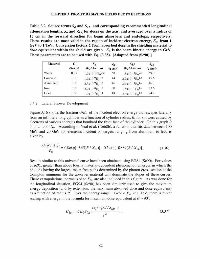
CHAPTER 3 PROMPT RADIATION FIELDS DUE TO ELECTRONS
62
Table 3.2 Source terms Sa and S15, and corresponding recommended longitudinal attenuation lengths, λλλλa and λλλλ15, for doses on the axis, and averaged over a radius of 15 cm in the forward direction for beam absorbers and end-stops, respectively. These results are most valid in the region of incident electron energy, Eo, from 1 GeV to 1 TeV. Conversion factors C from absorbed dose in the shielding material to dose equivalent within the shield are given. Eo is the beam kinetic energy in GeV. These parameters are to be used with Eq. (3.35). [Adapted from (Sc90).]
Material C Sa λλλλa S15 λλλλ15
(Sv/Gy) (Gy/electron) (g cm-2) (Gy/electron) (g cm-2) Water 0.95 1.9x10⁻¹⁰Eo2.0 58 1.5x10⁻¹¹Eo2.0 59.9
Concrete 1.2 1.9x10⁻⁹Eo1.8 44 2.2x10⁻¹¹Eo1.8 45.6
Aluminum 1.2 2.3x10⁻⁹Eo1.7 46 3.4x10⁻¹¹Eo1.7 46.3
Iron 1.3 2.9x10⁻⁸Eo1.7 30 1.8x10⁻¹⁰Eo1.7 33.6
Lead 1.8 1.9x10⁻⁷Eo1.4 18 4.6x10⁻¹⁰Eo1.4 24.2
3.4.2 Lateral Shower Development Figure 3.16 shows the fraction U/Eo of the incident electron energy that escapes laterally from an infinitely long cylinder as a function of cylinder radius, R, for showers caused by electrons of various energies that bombard the front face of the cylinder. On this graph R is in units of Xm. According to Neal et al. (Ne68b), a function that fits data between 100 MeV and 20 GeV for electrons incident on targets ranging from aluminum to lead is given by
U R X
ER X R Xm
m m( / )
. exp[ . ( / )] . exp[ . ( / )]0
0 8 345 0 2 0889= − + − . (3.36)
Results similar to this universal curve have been obtained using EGS4 (Sc90). For values of R/Xm greater than about four, a material-dependent phenomenon emerges in which the photons having the largest mean free paths determined by the photon cross section at the Compton minimum for the absorber material will dominate the slopes of these curves. These extrapolations, normalized to Xm, are also included in this figure. As was done for the longitudinal situation, EGS4 (Sc90) has been similarly used to give the maximum energy deposition (and by extension, the maximum absorbed dose and dose equivalent) as a function of radius R. Over the energy range 1 GeV < Eo < 1 TeV, there is direct scaling with energy in the formula for maximum dose equivalent at θ ≈ 90o;
20
)/ exp(
r
dSCEH
latlatlat
λρ−= , (3.37)
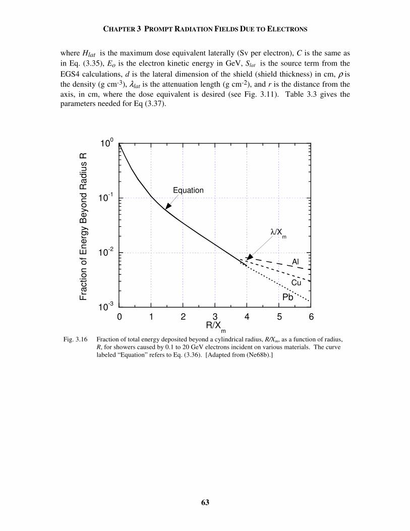
CHAPTER 3 PROMPT RADIATION FIELDS DUE TO ELECTRONS
63
where Hlat is the maximum dose equivalent laterally (Sv per electron), C is the same as in Eq. (3.35), Eo is the electron kinetic energy in GeV, Slat is the source term from the EGS4 calculations, d is the lateral dimension of the shield (shield thickness) in cm, ρ is the density (g cm-3), λlat is the attenuation length (g cm-2), and r is the distance from the axis, in cm, where the dose equivalent is desired (see Fig. 3.11). Table 3.3 gives the parameters needed for Eq (3.37).
10-3
10-2
10-1
100
0 1 2 3 4 5 6
Frac
tion
of E
nerg
y B
eyon
d R
adiu
s R
R/Xm
Equation
Al
Cu
Pb
λ/Xm
Fig. 3.16 Fraction of total energy deposited beyond a cylindrical radius, R/Xm, as a function of radius,
R, for showers caused by 0.1 to 20 GeV electrons incident on various materials. The curve labeled “Equation” refers to Eq. (3.36). [Adapted from (Ne68b).]
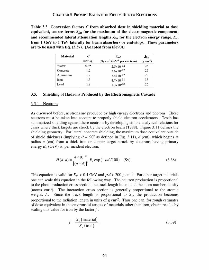
CHAPTER 3 PROMPT RADIATION FIELDS DUE TO ELECTRONS
64
Table 3.3 Conversion factors C from absorbed dose in shielding material to dose equivalent, source terms Slat for the maximum of the electromagnetic component, and recommended lateral attenuation lengths λλλλlat for the electron energy range, Eo, from 1 GeV to 1 TeV laterally for beam absorbers or end-stops. These parameters are to be used with Eq. (3.37). [Adapted from (Sc90).]
Material C Slat λλλλlat
(Sv/Gy) (Gy cm2 GeV-1 per electron) (g cm-2) Water 0.95 2.5x10⁻¹² 26 Concrete 1.2 3.6x10⁻¹² 27 Aluminum 1.2 3.4x10⁻¹² 29 Iron 1.3 4.7x10⁻¹¹ 33 Lead 1.8 1.3x10⁻¹⁰ 26
3.5. Shielding of Hadrons Produced by the Electromagnetic Cascade 3.5.1 Neutrons As discussed before, neutrons are produced by high energy electrons and photons. These neutrons must be taken into account to properly shield electron accelerators. Tesch has summarized shielding against these neutrons by developing simple analytical relations for cases where thick targets are struck by the electron beam (Te88). Figure 3.11 defines the shielding geometry. For lateral concrete shielding, the maximum dose equivalent outside of shield thickness (implying θ ≈ 90o as defined in Fig. 3.11), d (cm), which begins at radius a (cm) from a thick iron or copper target struck by electrons having primary energy Eo (GeV) is, per incident electron,
[ ]
( )13
2
4 10( , ) exp /100
( )oH d a E d
a dρ
−×= −+
(Sv). (3.38)
This equation is valid for Eo > 0.4 GeV and ρ d > 200 g cm-2. For other target materials one can scale this equation in the following way. The neutron production is proportional to the photoproduction cross section, the track length in cm, and the atom number density (atoms cm-3). The interaction cross section is generally proportional to the atomic weight, A. Since the track length is proportional to Xo, the production becomes proportional to the radiation length in units of g cm-2. Thus one can, for rough estimates of dose equivalent in the environs of targets of materials other than iron, obtain results by scaling this value for iron by the factor f ;
( )
( )material
irono
o
Xf
X= . (3.39)
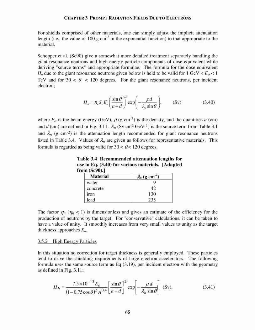
CHAPTER 3 PROMPT RADIATION FIELDS DUE TO ELECTRONS
65
For shields comprised of other materials, one can simply adjust the implicit attenuation length (i.e., the value of 100 g cm-2 in the exponential function) to that appropriate to the material. Schopper et al. (Sc90) give a somewhat more detailed treatment separately handling the giant resonance neutrons and high energy particle components of dose equivalent while deriving "source terms" and appropriate formulae. The formula for the dose equivalent Hn due to the giant resonance neutrons given below is held to be valid for 1 GeV < Eo < 1 TeV and for 30 < θ < 120 degrees. For the giant resonance neutrons, per incident electron;
2
sinexp
sinn n n on
dH S E
a dθ ρη
λ θ = − +
, (Sv) (3.40)
where Eo is the beam energy (GeV), ρ (g cm-3) is the density, and the quantities a (cm) and d (cm) are defined in Fig. 3.11. Sn (Sv cm2 GeV-1) is the source term from Table 3.1 and λn (g cm-2) is the attenuation length recommended for giant resonance neutrons listed in Table 3.4. Values of λn are given as follows for representative materials. This formula is regarded as being valid for 30 < θ < 120 degrees.
Table 3.4 Recommended attenuation lengths for use in Eq. (3.40) for various materials. [Adapted from (Sc90).]
Material λλλλn (g cm-2) water 9 concrete 42 iron 130 lead 235
The factor ηn (ηn < 1) is dimensionless and gives an estimate of the efficiency for the production of neutrons by the target. For "conservative" calculations, it can be taken to have a value of unity. It smoothly increases from very small values to unity as the target thickness approaches Xo. 3.5.2 High Energy Particles In this situation no correction for target thickness is generally employed. These particles tend to drive the shielding requirements of large electron accelerators. The following formula uses the same source term as Eq (3.19), per incident electron with the geometry as defined in Fig. 3.11;
( )
−
+−
×=
−
θλρθ
θ sin
expsin
cos75.01
105.7 2
4.02
13
h
oh
ddaA
EH (Sv). (3.41)
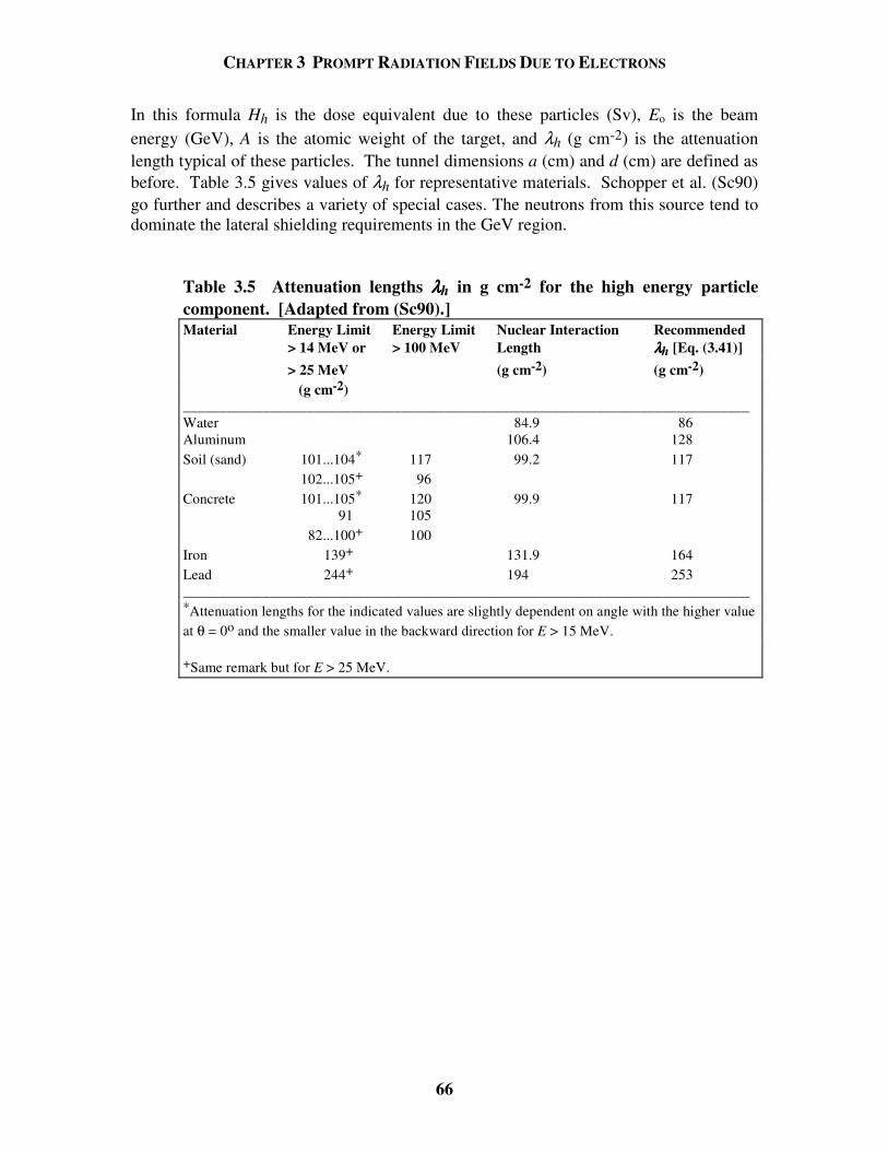
CHAPTER 3 PROMPT RADIATION FIELDS DUE TO ELECTRONS
66
In this formula Hh is the dose equivalent due to these particles (Sv), Eo is the beam energy (GeV), A is the atomic weight of the target, and λh (g cm-2) is the attenuation length typical of these particles. The tunnel dimensions a (cm) and d (cm) are defined as before. Table 3.5 gives values of λh for representative materials. Schopper et al. (Sc90) go further and describes a variety of special cases. The neutrons from this source tend to dominate the lateral shielding requirements in the GeV region.
Table 3.5 Attenuation lengths λλλλh in g cm-2 for the high energy particle component. [Adapted from (Sc90).] Material Energy Limit Energy Limit Nuclear Interaction Recommended > 14 MeV or > 100 MeV Length λλλλh [Eq. (3.41)] > 25 MeV (g cm-2) (g cm-2) (g cm-2) ______________________________________________________________________________ Water 84.9 86 Aluminum 106.4 128 Soil (sand) 101...104* 117 99.2 117 102...105+ 96 Concrete 101...105* 120 99.9 117 91 105 82...100+ 100 Iron 139+ 131.9 164 Lead 244+ 194 253 ______________________________________________________________________________ *Attenuation lengths for the indicated values are slightly dependent on angle with the higher value at θ = 0o and the smaller value in the backward direction for E > 15 MeV. +Same remark but for E > 25 MeV.
CHAPTER 3 PROMPT RADIATION FIELDS DUE TO ELECTRONS
67
Problems 1. An electron accelerator has a beam profile in the form of a 2 mm diameter circle
uniformly illuminated by the beam. Make a crude plot of the value of the dose equivalent rate in the beam as the energy increases from 1 MeV to 10 GeV. The average beam current is 1 microamp (1 µA). Assume the beam profile is unchanged during acceleration. Compare the results with Swanson’s simple formula, said to be a “conservative” value. Is his formula “conservative” above 100 MeV? (Hint: use Fig. 1.4.)
2. Calculate for electrons the critical energy and length of material that corresponds
to the radiation length for carbon and for lead. What does this say about the effectiveness of low-Z versus high-Z shielding materials for electrons?
3. A 100 MeV electron accelerator produces a 1.0 µA beam incident on a high-Z
(thick) target. Estimate the bremsstrahlung absorbed dose rates at θ = 0o and 90o at r = 2 m from the target using Swanson’s rules of thumb. Compare the 0o result with the “in-the-beam dose equivalent rate” found in Problem 1. How do the bremsstrahlung and in-beam dose rates compare?
4. Suppose the Tevatron enclosure at Fermilab is converted into an enclosure for an
electron synchrotron. The radius of the synchrotron is 1000 m. If the circulating beam is 1012 electrons, calculate the median energy of the synchrotron radiation photons for E0 = 100 GeV. Also find θc of the “lobe.”
5. For the accelerator of Problem 3, calculate the neutron flux density at r = 2 m
from giant resonance neutrons at large angles using the values in Table 3.1 for a high-Z (tungsten) target. Also use Table 3.1 to estimate the dose equivalent r = 2 m. Check this result by “guessing” the average neutron energy is between 1 and 10 MeV and use the curve in Fig. 1.5. Compare this neutron dose with the bremsstrahlung dose at large angles obtained in Problem 3.
6. For a 20 GeV electron accelerator operating at 1 kW, the electron beam strikes a
beam stop made of aluminum or iron. How long (in z) does the beam stop have to be to range out all of the muons for either aluminum or iron based on the mean range? Compare the dose equivalent rates at the immediate downstream ends of each material if 10 % of the muons leak through due to straggling and multiple Coulomb scattering can be neglected. (Assume the production of muons from Fe is approximately equal to that from Al. Recall the inverse square law.)
CHAPTER 3 PROMPT RADIATION FIELDS DUE TO ELECTRONS
68
7. In the discussion of the longitudinal development of electromagnetic showers, there are two different formulations (Rossi-Griesen, Bathow, and Van Ginneken). Using Van Ginneken's scaling method, calculate the value of ζ (g cm-2) for Eo = 1000 MeV, 10 GeV, and 100 GeV for copper and lead. Determine the number of radiation lengths to which ζ, corresponds for each material at each energy.
8. Compare the results of Van Ginneken for the location of the longitudinal shower
maximum with Bathow's result for copper and lead at the three energies given in Problem 7 for incident electrons. Is the agreement better or worse as the energy increases?
9. A hypothetical electron accelerator operates at either 100 MeV or 10 GeV and
delivers a beam current of 1 µA. Using Table 3.2, calculate the dose equivalent rates in both Sv/sec and rem/h at the end of a 300 cm long aluminum beam stop; averaged over a 15 cm radius that are due to bremsstrahlung. (The beam stop is a cylinder much larger than 15 cm in radius.) Then assume that, in order to save space, a high-Z beam stop is substituted. How long of a high-Z beam stop is needed to achieve the same dose rates? (Assume lead is a suitable high-Z material.) Why is the length of high-Z shield different for the 2 energies? In this problem, assume the values in Table 3.2 are valid for energies as low as 0.1 GeV.
10. In the accelerator and beam stop of Problem 9, if the radius of the beam stop is 30
cm, what is the maximum dose equivalent rate (Sv s-1 and rem h-1) on the lateral surface (at contact at r = 30 cm) of the beam stop for both energies, 100 MeV and 10 GeV, and both materials? Again assume approximate validity at 100 MeV of the results.
11. Calculate the dose equivalent rate due to neutrons outside a 1 meter thick concrete
shield surrounding a cylindrical tunnel (inner radius 1 meter) in which is located a copper target stuck by 1 µA beam of 100 GeV electrons. The geometry should be assumed to be optimized for producing giant resonance photoneutrons and the calculations should be performed at θ = 30, 60 and 90o (Concrete has ρ = 2.5 g cm-3). Express the result as Sv s-1 and rem h-1. For θ = 90o, use Eq. (3.38) as a check.
CHAPTER 4 PROMPT RADIATION FIELDS DUE TO PROTONS AND IONS
69
4.1 Introduction In this chapter the major features of development of prompt radiation fields and the shielding of these fields as they are produced at proton and ion accelerators are addressed. Particular emphasis is placed on the shielding of neutrons in view of their general dominance of the radiation fields. The shielding of muons at such accelerators is also described. Methods for utilizing the results of both semi-empirical and Monte Carlo methods in the solution of practical shielding problems are presented. 4.2 Radiation Production by Proton Accelerators 4.2.1 The Direct Beam; Radiation Hazards and Nuclear Interactions Direct beams at proton accelerators, from the dosimetric standpoint, nearly always dominate over any type of secondary phenomena in terms of the level of hazard since the beam current is generally confined to small dimensions. Figure 1.4 gives the dose equivalent per fluence as a function of proton energy. The physical reason that the conversation factor shows such a prominent transition at about 200 MeV is that below that energy the proton range in tissue is less than the typical thickness of the human body. At these lower energies, a high fraction of the proton’s energy is absorbed in tissue. However, as the energy is increased above 200 MeV, an increasing fraction of the proton’s energy escapes from the body so that it requires a far larger fluence of protons to deliver the same absorbed dose or dose equivalent. The ionization range of a proton increases monotonically with energy. Since the mass of the proton is so much larger than that of the electron, the radiative processes of bremsstrahlung and synchrotron radiation are negligible at energies found at current accelerators, but not at future ones that reach ultra-high energies. As will be discussed in Section 4.5, the cross sections for inelastic interactions become nearly independent of energy and have approximately the values tabulated in Table 1.2. Thus, as an individual proton passes through a material medium, the probability of it participating in an inelastic nuclear reaction before it loses its remaining energy to ionization becomes significant and, as the energy increases, the dominant means by which protons are absorbed. Tesch has summarized this effect and the results are shown in Fig. 4.1 for various materials and energies (Te85). 4.2.2 Neutrons (and Other Hadrons at High Energies) The production and behavior of neutrons at proton and ion accelerators have different characteristics as the energy of the beam particles, Eo, is increased. The interactions of protons in a sequence of energy domains of proton energy will be discussed separately.
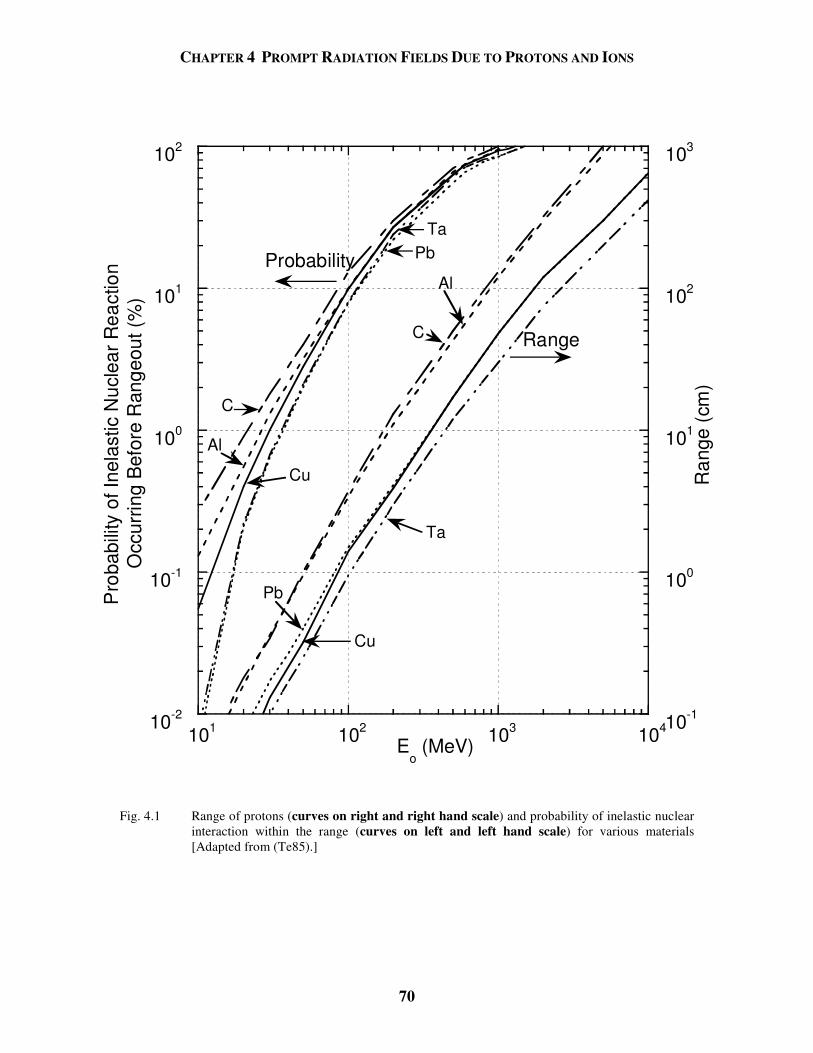
CHAPTER 4 PROMPT RADIATION FIELDS DUE TO PROTONS AND IONS
70
10-2
10-1
100
101
102
10-1
100
101
102
103
101 102 103 104
Pro
babi
lity
of In
elas
tic N
ucle
ar R
eact
ion
Occ
urrin
g B
efor
e R
ange
out (
%)
Ran
ge (
cm)
Eo (MeV)
Probability
Range
C
C
Al
Al
Cu
Cu
Ta
Ta
Pb
Pb
Fig. 4.1 Range of protons (curves on right and right hand scale) and probability of inelastic nuclear
interaction within the range (curves on left and left hand scale) for various materials [Adapted from (Te85).]
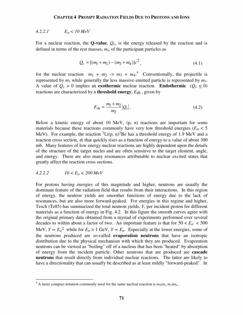
CHAPTER 4 PROMPT RADIATION FIELDS DUE TO PROTONS AND IONS
71
4.2.2.1 Eo < 10 MeV For a nuclear reaction, the Q-value, Qv, is the energy released by the reaction and is defined in terms of the rest masses, mi, of the participant particles as Q m m m m cv = + − +[( ) ( )]1 2 3 4
2, (4.1)
for the nuclear reaction m1 + m2 -> m3 + m4.9 Conventionally, the projectile is represented by m1 while generally the less massive emitted particle is represented by m3. A value of Qv > 0 implies an exothermic nuclear reaction. Endothermic (Qv < 0) reactions are characterized by a threshold energy, Eth , given by
Em m
mQth v=
+1 2
2. (4.2)
Below a kinetic energy of about 10 MeV, (p, n) reactions are important for some materials because these reactions commonly have very low threshold energies (Eth < 5 MeV). For example, the reaction 7Li(p, n)7Be has a threshold energy of 1.9 MeV and a reaction cross section, σ, that quickly rises as a function of energy to a value of about 300 mb. Many features of low energy nuclear reactions are highly dependent upon the details of the structure of the target nuclei and are often sensitive to the target element, angle, and energy. There are also many resonances attributable to nuclear excited states that greatly affect the reaction cross sections. 4.2.2.2 10 < Eo < 200 MeV For protons having energies of this magnitude and higher, neutrons are usually the dominant feature of the radiation field that results from their interactions. In this region of energy, the neutron yields are smoother functions of energy due to the lack of resonances, but are also more forward-peaked. For energies in this regime and higher, Tesch (Te85) has summarized the total neutron yields, Y, per incident proton for different materials as a function of energy in Fig. 4.2. In this figure the smooth curves agree with the original primary data obtained from a myriad of experiments performed over several decades to within about a factor of two. An important feature is that for 50 < Eo < 500 MeV, Y ∝ Eo2 while for Eo > 1 GeV, Y ∝ Eo. Especially at the lower energies, some of the neutrons produced are so-called evaporation neutrons that have an isotropic distribution due to the physical mechanism with which they are produced. Evaporation neutrons can be viewed as "boiling" off of a nucleus that has been "heated" by absorption of energy from the incident particle. Other neutrons that are produced are cascade neutrons that result directly from individual nuclear reactions. The latter are likely to have a directionality that can usually be described as at least mildly "forward-peaked". In
9 A more compact notation commonly used for the same nuclear reaction is m2(m1, m3)m4.
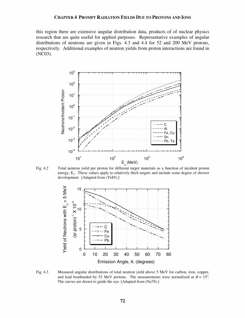
CHAPTER 4 PROMPT RADIATION FIELDS DUE TO PROTONS AND IONS
72
this region there are extensive angular distribution data, products of of nuclear physics research that are quite useful for applied purposes. Representative examples of angular distributions of neutrons are given in Figs. 4.3 and 4.4 for 52 and 200 MeV protons, respectively. Additional examples of neutron yields from proton interactions are found in (NC03).
10-4
10-3
10-2
10-1
100
101
102
103
101 102 103 104
CAlFe, CuSnPb, Ta
Neu
trons
/Inci
dent
Pro
ton
Eo (MeV)
Fig. 4.2 Total neutron yield per proton for different target materials as a function of incident proton energy, Eo. These values apply to relatively thick targets and include some degree of shower development. [Adapted from (Te85).]
0
5
10
15
0 10 20 30 40 50 60 70 80
CFeCuPb
Yie
ld o
f Neu
tron
s w
ith E
n > 5
MeV
(sr p
roto
n)-1
X 1
0-4
Emission Angle, θ, (degrees)
Fig. 4.3 Measured angular distributions of total neutron yield above 5 MeV for carbon, iron, copper, and lead bombarded by 52 MeV protons. The measurements were normalized at θ = 15o. The curves are drawn to guide the eye. [Adapted from (Na78).]

CHAPTER 4 PROMPT RADIATION FIELDS DUE TO PROTONS AND IONS
73
10-8
10-7
10-6
10-5
10-4
10-3
0 50 100 150 200
dY/d
ΩdE
(N
eutro
ns M
eV-1
sr-1
per
inci
dent
pro
ton)
Neutron Energy (MeV)
Fe
Al
Fe
Fe
Fe
Al
Al
Al
90 < θ < 180o60 < θ < 90o
30 < θ < 60o
0 < θ < 30o
Fig. 4.4 Calculated energy spectra of neutrons emitted by iron and aluminum targets bombarded by
200 MeV protons for four ranges of θ. The results for iron are from (Ha88) while those for aluminum are from (Al75). [Adapted from (Ha88).]
CHAPTER 4 PROMPT RADIATION FIELDS DUE TO PROTONS AND IONS
74
4.2.2.3 200 MeV < Eo < 1 GeV; ("Intermediate" Energy) In this region, many more reaction channels become open and the number of protons emitted gradually becomes approximately equal to the number of neutrons. In fact, at the highest energies the radiation effects of protons and neutrons are essentially identical and both must be taken into account. Thus reliance on the values shown in Fig. 4.2 could underestimate radiation effects by as much as a factor of two. Also, at these energies, cascade neutrons become much more important than evaporation neutrons and thus the radiation field is more sharply forward-peaked with increasing primary particle energy. 4.2.2.4 Eo > 1 GeV ("High" Energy Region) In this region, both the calculations and measurements become much more difficult. Figures 4.5, 4.6, 4.7, and 4.8 show representative data at 14, 26, 22, and 225 GeV.10 These results should be regarded as thin target values. "Thin" target in this context means a target shorter than the mean free path for removal of the high energy protons. Table 4.1 summarizes common removal mean free paths based upon the nuclear collision lengths of Table 1.2. Considerable efforts have been made to semi-empirically fit the distributions of the yields of secondary particles produced by proton interactions. These efforts are needed to supply the needs of the particle physics community as well as to address radiation safety issues. They began in the early days of radiation protection and continue to the present and are embodied in the continual development of Monte Carlo programs designed to calculate the properties of hadronic cascades as discussed in Section 4.6. An example of a particularly successful early model is one developed by Ranft (Ra67) expressed as the following formula for the yield of protons (or neutrons):
22 2
2 21 ( ) 1 1 ( ) 1 exp( )o oo o
o o p
p ppd Y A Bpf p f p p Cp
d dp p p p mθ
= + + − × + − − Ω
(protons or neutrons sr-1 GeV-1 per interacting proton), (4.3) where po is the primary proton momentum (GeV/c), mp is the proton rest energy (GeV/c2), f (p0) = 1 + (po/mp)21/2, and
θ is the production angle (radians). The parameters A, B, and C of the Ranft model are material dependent and are given in Table 4.2. According to Patterson and Thomas (Pa73), when this formula is numerically integrated above the indicated particle threshold, it describes well the experimental data presented in Figs. 4.7 and 4.8. 10 Much of the experimental data presented in this and other sections related to high energy interactions were obtained using activation "threshold" detectors. This technique will be discussed at greater length in Section 9.5.3.
CHAPTER 4 PROMPT RADIATION FIELDS DUE TO PROTONS AND IONS
75
10-2
10-1
100
101
102
0 20 40 60 80 100
14 GeV Protons26 GeV Protons
dY/d
Ω fo
r En >
20 M
eV p
er p
roto
n (s
r-1)
θ (degrees) Fig. 4.5 Measurements of the angular distribution, dY/dΩ, of neutrons above 20 MeV produced by 14
and 26 GeV protons incident on a thin beryllium target. The yield is per interacting proton. The lines are drawn to guide the eye. [Adapted from (Gi68).]
10 -5
10 -4
10 -3
10 -2
10 -1
100
101
102
0 20 40 60 80 100
14 GeV Protons26 GeV Protons
dY/d
Ω fo
r En >
600
MeV
per
pro
ton
(sr-1
)
θ (degrees) Fig. 4.6 Measurements of the angular distribution, dY/dΩ, of neutrons above 600 MeV produced by 14
and 26 GeV protons incident on a thin beryllium target. The yield is per interacting proton. The lines are drawn to guide the eye [Adapted from (Gi68).]
CHAPTER 4 PROMPT RADIATION FIELDS DUE TO PROTONS AND IONS
76
10-7
10-6
10-5
10-4
10-3
10-2
0 20 40 60 80 100 120 140 160
Ehadron
> 35 MeV
Ehadron
> 85 MeV
Ehadron
> 600 MeV
Had
ron
Flue
nce
at 1
met
er
(cm
-2 p
er in
tera
ctin
g pr
oton
)
θ (degrees)
Fig. 4.7 Measured angular distributions of hadron fluence (particles cm-2) at 1 meter from a copper target bombarded by 22 GeV protons. Several choices of hadron energy thresholds are shown. [Adapted from (Ra72).]
10-2
100
102
104
106
0 20 40 60 80 100 120 140 160
Had
ron
Yie
ld p
er In
cide
nt P
roto
n (s
r-1)
θ (degrees)
50 MeV x 105
70 MeV x 104
105 MeV x 103
126 MeV x 102
393 MeV x 101561 MeV
Fig. 4.8 Measurements of hadron yields above different energy thresholds as a function of production
angle θ around a 15 cm long copper target bombarded by 225 GeV protons. The data have been multiplied by the indicated powers of 10 prior to plotting. The lines are intended to guide the eye. [Adapted from (St85).]
CHAPTER 4 PROMPT RADIATION FIELDS DUE TO PROTONS AND IONS
77
Table 4.1 Summary of removal mean free paths for high energy protons. [Adapted from Table 1.2.]
Table 4.2 Material-dependent parameters to be used in Eq. 4.3. [From (Ra67).] Target A B C H2 0.55 -0.30 2.68 Be 0.68 -0.39 3.12 Fe 0.92 -0.75 2.90 Pb 1.14 -1.06 2.73
4.2.3 Sullivan's Formula For simple radiation protection calculations, Sullivan (Su89) has developed a formula for the fluence, Φ (θ ), of hadrons with Eo > 40 MeV that will be produced at one meter from a copper target struck by protons in the energy region 5 < Eo < 500 GeV per interacting proton;
( )[ ]
ΦΕ
( )/
θθ
=+
1
2 35 02 (cm-2 per interacting proton), (4.4)
where Eo is in GeV and θ is in degrees. At proton energies between about 0.05 and 5 GeV, this formula also approximately
Material Density Removal Mean Removal Mean Free Path Free Path
(grams cm-3) (grams cm-2) (cm)
hydrogen gas @ STP 9.00 x 10⁻⁵ 43.3 4.81 x 10⁵
beryllium 1.85 55.8 30.16 carbon 2.27 60.2 26.58 aluminum 2.70 70.6 26.15 iron 7.87 82.8 10.52 copper 8.96 85.6 9.55 lead 11.35 116.2 10.24 uranium 18.95 117.0 6.17 air @ STP 1.29 x 10⁻³ 62.0 4.81 x 10⁴
water 1.00 60.1 60.10 concrete (typical) 2.50 67.4 26.96 silicon dioxide (quartz) 2.64 66.5 25.19 plastics (polyethylene) 0.93 56.9 61.29
CHAPTER 4 PROMPT RADIATION FIELDS DUE TO PROTONS AND IONS
78
accounts for the distributions of neutrons per incident proton. This equation is plotted in Fig. 4.9, for “lateral" (θ ≈ 90o) and "forward" (θ ≈ 0o) directions.
10-6
10-5
10-4
10-3
10-2
10-1
100
10-2 10-1 100 101 102 103
Forward (θ = 0o)
Lateral (θ = 90o)
Flue
nce
at 1
met
er
per I
nter
actin
g P
roto
n (c
m-2
)
Proton Energy (GeV)
Fig. 4.9 Plot of Eq. (4.4) for two different values of θ. The proton is interacting in a copper target. [According to (Su89).]
Of course, the dose equivalent is more directly germane to radiation protection concerns than is the "raw" fluence. In principle, the dose equivalent can be obtained by integrating over the spectrum the product of the fluence and the dose equivalent per unit fluence, P(E), defined in Section 1.2.1;
max
0( ) ( )
EH dEP E E= Φ , (4.5)
or by summation, taking into account the "coarseness" of available data and/or calculations;
1
( ) ( ) ( )m
j j jj
H E P E E=
= ∆ Φ . (4.6)
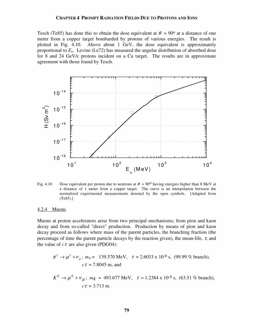
CHAPTER 4 PROMPT RADIATION FIELDS DUE TO PROTONS AND IONS
79
Tesch (Te85) has done this to obtain the dose equivalent at θ = 90o at a distance of one meter from a copper target bombarded by protons of various energies. The result is plotted in Fig. 4.10. Above about 1 GeV, the dose equivalent is approximately proportional to Eo. Levine (Le72) has measured the angular distribution of absorbed dose for 8 and 24 GeV/c protons incident on a Cu target. The results are in approximate agreement with those found by Tesch.
10 -18
10 -17
10 -16
10 -15
10 -14
10 1 10 2 10 3 10 4
H (
Sv
m2 )
Eo (M eV)
Fig. 4.10 Dose equivalent per proton due to neutrons at θ = 90o having energies higher than 8 MeV at
a distance of 1 meter from a copper target. The curve is an interpolation between the normalized experimental measurements denoted by the open symbols. [Adapted from (Te85).]
4.2.4 Muons Muons at proton accelerators arise from two principal mechanisms; from pion and kaon decay and from so-called "direct" production. Production by means of pion and kaon decay proceed as follows where mass of the parent particles, the branching fraction (the percentage of time the parent particle decays by the reaction given), the mean-life, τ, and the value of cτ are also given (PDG04):
µνµπ +→ ±± ; mπ = 139.570 MeV, τ = 2.6033 x 10⁻⁸ s, (99.99 % branch),
cτ = 7.8045 m, and K ± ±→ +µ ν µ ; mK = 493.677 MeV, τ = 1.2384 x 10⁻⁸ s, (63.51 % branch),
cτ = 3.713 m.
CHAPTER 4 PROMPT RADIATION FIELDS DUE TO PROTONS AND IONS
80
"Direct" muon production, important only at very high energy hadron accelerators, is discussed in more detail in Section 4.7.3. Muon fields are forward-peaked and, normally, dominated by those from pion decay, except, perhaps at the highest energies. Usually, Monte Carlo techniques are needed to accurately estimate muon intensities. This is because of the need to:
• calculate the production of pions from the proton interactions,
• follow the pions until they decay or interact,
• adequately account for the range-energy relation and range straggling, and
• track the muons to the point of interest, for example, through magnetic fields. 4.3 Primary Radiation Fields at Ion Accelerators Large portions of Section 4.2 have discussed general considerations that are appropriate the primary radiation fields generated by accelerated ions as well as to protons. In this section, special issues found in radiation fields produced by ions other than protons are described. Because the ionization range for ions of a given kinetic energy decreases as a function of ion mass, targets become effectively "thicker" as the ion mass increases. A comprehensive recent reference on this topic is that of Nakamura and Heilbronn (Na05) 4.3.1 Light Ions (Ion Mass Number A < 5) For such ions there are exothermic reactions that should be treated as special cases. Noteworthy examples (followed by their reaction Q-values, Qv, in parentheses) are; D(d, n)3He (Qv = 3.266 MeV), 9Be(α, n)12C (Qv = 5.708 MeV), and 3H(d, n)4He (Qv = 17.586 MeV). In some cases monoenergetic beams of neutrons can be produced using these or the following slightly endothermic reactions: 12C(d, n)13N (Qv = -0.281 MeV), T(p, n)3He (Qv = -0.764 MeV), and 7Li(p, n)7Be (Qv = -1.646 MeV). The energies of such neutrons can range from 0 to 24 MeV for bombarding energies up to 10 MeV. In general, deuteron stripping and breakup reactions, (d, n), have the highest yields

CHAPTER 4 PROMPT RADIATION FIELDS DUE TO PROTONS AND IONS
81
because the binding energy of the deuteron is only 2.225 MeV. In effect, one gets an extra neutron "for free". Furthermore, the neutrons due to deuteron stripping reactions typically have a kinetic energy of about half that of the incident deuteron if the latter has a kinetic energy that is large compared with the binding energy of the target nucleus. This phenomenon is especially pronounced at the lower energies. In the low energy region, and especially with light ions, one should carefully consider all possible reactions given the materials present in conjunction with the ions that are being accelerated. Patterson and Thomas (Pa73) have summarized total neutron yields for light ions. In general, the yields for the various light ions behave similarly to those due to protons. That is, the yield is within, typically, a factor of three of that expected for proton beams. A good measurement of neutron yields due to 40 MeV α-particles has been provided by Shin et al. (Sh95). Higher energy neutron production data for 640 and 710 MeV α-particles has been provided by Cecil et al. (Ce80). 4.3.2 Heavy Ions (Ions with A > 4) At higher energies and especially at higher masses, neutron yield and dose equivalent data and calculations are very sparse. The data is usually normalized in terms of kinetic energy per atomic mass unit, the specific energy, expressed in units of MeV/amu, or kinetic energy per nucleon because reaction parameters generally scale to that parameter. In the literature the technical distinction between energy/amu and energy/nucleon is often ignored. In the range up to 20 MeV/amu, Ohnesorge et al. (Oh80) have measured dose equivalent rates at one meter at θ = 90o from thick targets of iron, nickel, or copper bombarded by 4He, 12C, 14N, 16O, and 20Ne beams. The dose equivalent was found to be essentially independent of ion type as a function of specific energy. At 10 MeV/amu, a value of 6.3 x 10⁻¹⁸ Sv/incident ion was measured while at 20 MeV/amu, a value of 3.6 x 10⁻¹⁷ Sv/incident ion was found. Other data relevant to this general energy region are exemplified by those of Hubbard et al. (Hu60), Aleinikov et al. (Al85), and especially Nakamura (Na85). Tuyn et al. (Tu84) reported studies done with 86 MeV/amu 12C ions incident on Fe targets slightly thicker (longer) than an interaction length. The measurements are shown in Fig. 4.11. At a specific energy of 155 MeV/amu, Britvitch et al. (Br99) have measured energy spectra and total neutron yields and angular distributions for 4He, 12C, and 16O ions stopping in a thick target of an alloy of tungsten, nickel, and copper commonly known as “Hevimet”. The differential yields, dY/dΩ, were fit by the form
)exp( βθ−=Ω
CddY
, (4.7)
with the total yields being found by the integration,
[ ]20
exp( ) 1( )2 sin 2
( 1)total
dYY d C
d
π βπθπ θ θ πβ− +
= =Ω + . (4.8)
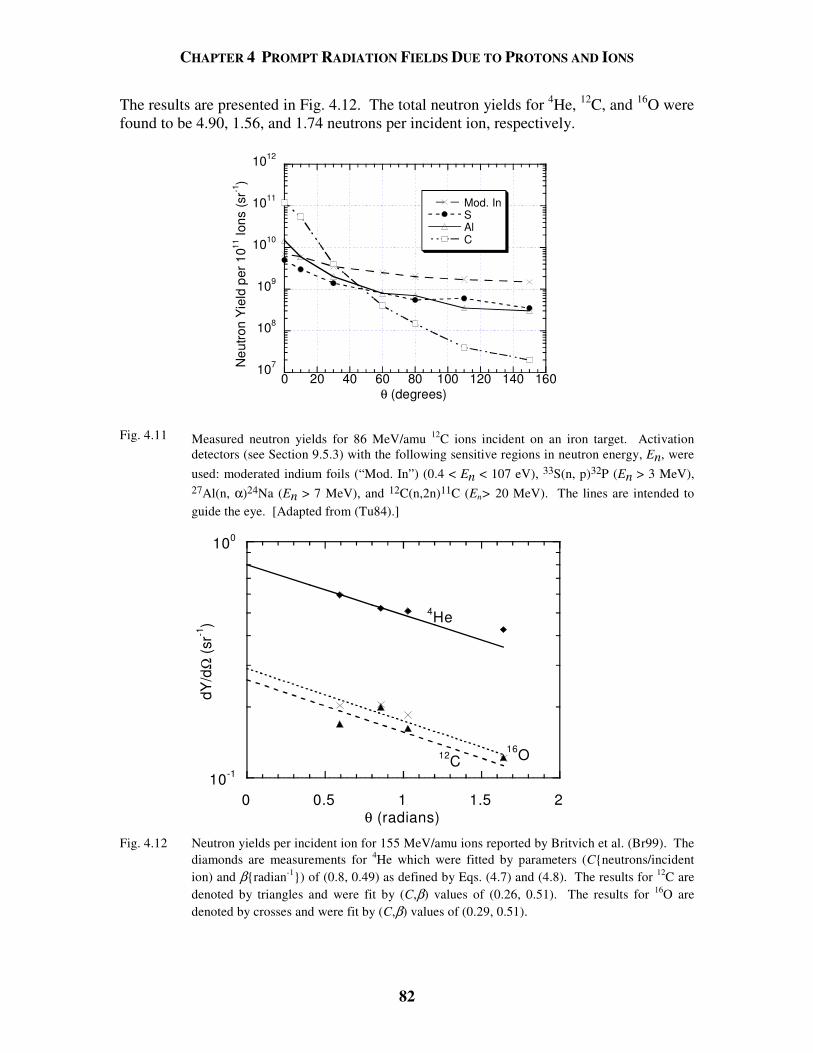
CHAPTER 4 PROMPT RADIATION FIELDS DUE TO PROTONS AND IONS
82
The results are presented in Fig. 4.12. The total neutron yields for 4He, 12C, and 16O were found to be 4.90, 1.56, and 1.74 neutrons per incident ion, respectively.
107
108
109
1010
1011
1012
0 20 40 60 80 100 120 140 160
Mod. InSAlC
Neu
tron
Yie
ld p
er 1
011 Io
ns (s
r-1)
θ (degrees)
Fig. 4.11 Measured neutron yields for 86 MeV/amu 12C ions incident on an iron target. Activation
detectors (see Section 9.5.3) with the following sensitive regions in neutron energy, En, were used: moderated indium foils (“Mod. In”) (0.4 < En < 107 eV), 33S(n, p)32P (En > 3 MeV), 27Al(n, α)24Na (En > 7 MeV), and 12C(n,2n)11C (En> 20 MeV). The lines are intended to guide the eye. [Adapted from (Tu84).]
10-1
100
0 0.5 1 1.5 2
dY/d
Ω (s
r-1)
θ (radians)
4He
12C16O
Fig. 4.12 Neutron yields per incident ion for 155 MeV/amu ions reported by Britvich et al. (Br99). The
diamonds are measurements for 4He which were fitted by parameters (Cneutrons/incident ion) and βradian-1) of (0.8, 0.49) as defined by Eqs. (4.7) and (4.8). The results for 12C are denoted by triangles and were fit by (C,β) values of (0.26, 0.51). The results for 16O are denoted by crosses and were fit by (C,β) values of (0.29, 0.51).
CHAPTER 4 PROMPT RADIATION FIELDS DUE TO PROTONS AND IONS
83
Clapier and Zaidins (Cl83) have surveyed a sample of ion data from 3 to 86 MeV/amu and have been able to approximate the total neutron yields an angular distributions over that domain. They found the total yield per ion, Y, to be given by ( )( , ) ( ) ZY W Z C Z W η= (neutrons ion-1) with (4.9a) η( ) .Z Z= 122 and (4.9b)
( ) 4
2
2.75
1.96 10( ) exp 0.475 lnC Z Z
Z
−×= − , (4.9c)
where Z is the atomic number of the projectile and W is the specific energy (MeV/amu). They found essentially no dependence on the atomic number of the target material and assert that an average neutron energy of 6-7 MeV is appropriate. To fit the angular distribution, dY/dΩ, the “form factor” F(θ, ξ) defined as follows was found to be useful:
2
1 1 1( , )
4 ln 1 1/ sin ( / 2)F θ ξ
π ξ ξ θ
= + + , (4.10)
where θ is defined as usual and the fitting parameter ξ is related to the ratio of fluences, Φ, at θ = 0 and 90 degrees, and thus related to “forward-peakedness”. In a subsequent paper, Aleinikov et al. (Al85) developed the following parameterization for ξ :
o o
) 1(0 ) ( ) (0 ) / ( ) 1
ξ Φ(90= =Φ − Φ 90 Φ Φ 90 −
. (4.11)
In this scheme, ( )
( , ) ( , )dY
Y W Z Fd
θ θ ξ=Ω
. (4.12)
Values of the parameters C(Z) and η(Z) for specific circumstances are given in Table 4.3. Table 4.3 Values of the parameters ηηηη(Z) and C(Z) as expressed in Eqs (4.9). [Adapted from (Cl83).]
Atomic Number Element ηηηη(Z) C(Z) 1 hydrogen 1.5 1.7 x 10⁻⁴
2 helium 2.6 3.9 x 10⁻⁶
6 carbon 1.7 2.5 x 10⁻⁶
8 oxygen 3.6 3.6 x 10⁻⁷
10 neon 7.0 2.7 x 10⁻¹⁰
18 argon 7.0 5.1 x 10⁻¹¹
36 krypton 7.9 6.0 x 10⁻¹²
82 lead 11.0 1.7 x 10⁻¹³
CHAPTER 4 PROMPT RADIATION FIELDS DUE TO PROTONS AND IONS
84
They also give a few examples of the values of their parameter, ξ ; 0.07 for uranium incident on uranium at 9 MeV/amu, 0.025 for neutrons of energy En < 20 MeV produced by 86 MeV/amu 12C incident on iron, and 3 x 10⁻⁴ for neutrons of energy En > 20 MeV produced by 86 MeV/amu 12C incident on iron (based on an analysis of the data presented in Fig. 4.11). One, in principle, could use values given in Table 4.3 or the direct calculation using Eqs. (4.9b) and (4.9c) and obtain some idea of the uncertainties inherent in this fit of such a broad range of data. However, the uncertainties in this type of fit are quite large due to the functional forms that were used. McCaslin et al. (McC85) measured the angular distribution of yields of 670 MeV/amu Ne and Si ions stopped in a copper target. The distributions for the two different projectiles were similar with fits to the data provided for the 670 MeV/amu 20Ne ions. For the 20Ne ions, including all neutrons above 6.5 MeV at a radius of one meter, McCaslin found
Φ( )θθ
= 3721
neutrons m-2 per ion for 2o < θ < 180o , θ in degrees (4.13)
and for the same ions, including all neutrons above 20 MeV;
Φ( )θ θ= 248e-0.2 neutrons m-2 per ion for 0o < θ < 20o, θ in degrees, and (4.14) Φ( )θ θ= 10e-0.038 neutrons m-2 per ion for 20o < θ < 120o, θ in degrees. (4.15) The neutron yields at this high specific energy for heavy ions turn out to be quite large. By integrating the above over all angles, one finds a total yield of 74.1 neutrons/incident ion for En > 6.5 MeV for 20Ne incident ions (see Problem 4). It is clear that a more complete picture of neutron yields from heavy ion interactions is desirable especially in the intermediate to high energy ranges. The systematic studies of Kurosawa et al. (Ku99), Heilbronn et al. (He99), and Kurosawa et al. (Ku00) that span the periodic table document major advances on this topic. Along with a good parameterizeration of measured neutron angular distributions not discussed in detail here, (Ku00) presents a useful simple formula based upon geometrical considerations that describes total yield, Y, of neutrons having energies above 5 MeV emitted into the hemisphere 0 < θ < 90o. This heavy ion neutron yield formula is
( )6 22 1/3 1/3
1/3 2
1.5 10 PP P T P
T P
AY W A A N
N Z
−×= + (neutrons particle-1), (4.16)
where the subscripts P and T denote properties of the projectile ion and the target, respectively, and Z, N, and A have their usual meanings of atomic number, neutron number, and mass number. WP is the projectile specific energy in MeV amu-1. This
CHAPTER 4 PROMPT RADIATION FIELDS DUE TO PROTONS AND IONS
85
formula describes data generally within factors of 2 or 3 for ions from He to Xe incident ions fully stopped in targets ranging from C to Pb over the specific energy domain 100 < EP < 800 MeV amu-1. Fig. 4.13 shows representative total neutron yields for heavy ions from some measurements and calculations using Eq. (4.16) compared with the yields found for protons as a function of specific energy.
10-3
10-2
10-1
100
101
102
101 102 103 104
Protons on Fe or Cu (Te83)12C on Cu (Hu60) or W (Br99)20Ne on Cu (McC85)
Eq. (4.16): 12C on Fe
Eq. (4.16): 20Ne on Cu
Eq. (4.16): 56Fe on Fe
Neu
trons
/Sto
pped
Ion
Specific Energy (MeV/amu)
Fig. 4.13 Neutron yields as a function of specific energy for selected projectiles and targets as reported by the cited references along with results obtained using Eq. (4.16).11
4.4 Hadron (Neutron) Shielding for Low Energy Incident Protons (Eo < 15 MeV) Neutron shielding in this region is especially complex because it is the region of significant nuclear structure effects. There are many resonances associated with compound nucleus that can be excited and there are also many nuclear reaction channels leading to a large number of nuclear excited states up to 20 MeV in excitation energy which have a wide variety of nuclear structure quantum numbers and very narrow widths in energy.
11 A comment should be made here that measurements of neutron yields using heavy ions are rather difficult to perform. This leads to results from different laboratories that sometimes appear to be in only “qualitative” agreement. For example, for the conditions of the measurement reported by McCaslin (McC85), using Eq. (4.16) a yield of only 18.6 neutrons ion-1 is calculated. The discrepancy of a factor of four is not likely attributable to the somewhat smaller angular range covered by Eq. (4.16). “Systematic” variables such as target sizes and neutron detection techniques may be quite important. At the higher energies, the escape of mesons produced by interactions in target volume may also be important.
CHAPTER 4 PROMPT RADIATION FIELDS DUE TO PROTONS AND IONS
86
Clark (Cl71) has expressed some general rules of attack on the neutron shielding problem. Clark’s principles are:
• "The shield must be sufficiently thick and the neutrons so distributed in energy that only a narrow band of the most penetrating source neutrons give any appreciable ultimate contribution to the dose outside the shield."
• "There must be sufficient hydrogen in the shield, intimately mixed or in the final
shield region, to assure a very short characteristic transport length from about one MeV to absorption at or near thermal energy."
• "The source energy distribution and shield material (non-hydrogeneous)
properties must be such as to assure a short transport distance for slowing down from the most penetrating energies to one MeV."
An elementary method used to calculate shielding thicknesses in this energy domain is that of removal cross section theory. It has been found that the dose equivalent, H, as a function of shield thickness, t, is approximately given for these neutrons by ( ) exp( )o rH t PG t= Φ −Σ , (4.17) where Φo is the fluence before the shielding (calculated from neutron yield information), P is the dose equivalent per fluence conversion factor (obtained by performing any needed integration over the energy spectrum), G is a "geometry factor", t (cm) is the thickness of the shield. For parallel beams, G = 1 while for an isotropic point source, G = 1/r2. Σr is the macroscopic removal cross section;
Σrr
A=
0 602. σ ρ (cm-1), (4.18)
where σr is the microscopic removal cross section in barns, ρ is the density (g cm-3) and A is the mass number. For mixtures of n materials,
ir ri
n
i
ρρ
= (4.19)
where the right-most quantity is the removal cross section per unit mass of the ith constituent and ρi is the partial density of the ith material. In this formulation the overall density is equal to the sum of the partial densities. For A > 8, σr ≈ 0.21 A-0.58 (barns) (4.20) for neutrons of approximately 8 MeV.
CHAPTER 4 PROMPT RADIATION FIELDS DUE TO PROTONS AND IONS
87
Figure 4.14 taken from (Pa73) shows the values of σr as a function of mass number at this energy. Table 4.4 gives representative values for σr for some energies where this approach is applicable.
10-2
10-1
10 100
σ r (ba
rns)
Mass Number, A Fig. 4.14 Removal cross sections per unit atomic mass number for fission neutrons as a function of
mass number at a neutron energy of 8 MeV. Over the range 8 < A < 240, the values are well fit by Eq. (4.20). [Adapted from (Pa73)].
Table 4.4 Removal cross sections, σσσσr (barns), for low energy neutrons. The typical accuracy is quoted to be + 5 %. [Adapted from (Pa73).] Element 1 MeV Fission
Spectrum 2.9 MeV 4 MeV 6.7 MeV 14.9 MeV
Carbon 0.9 1.58 1.05 0.83 0.50 Aluminum 1.31 Iron 1.1 1.96 1.94 1.98 2.26 1.60 Copper 2.04 Lead 3.28 2.70 3.44 3.77 2.95 The use of removal cross sections describe attenuation data rather effectively despite the fact that as more shielding is penetrated, neutrons of lower energy tend to dominate the spectrum over those found in the few MeV region.
CHAPTER 4 PROMPT RADIATION FIELDS DUE TO PROTONS AND IONS
88
4.5 Limiting Attenuation at High Energy The most important feature of neutron shielding at higher energy accelerators is the fact that the attenuation length becomes an approximate constant at high energy. As the energy increases, the neutron inelastic cross sections increase rapidly until about 25 MeV where they generally level off and then fall rapidly with energy in the region 25 < En < 100 MeV to a value which becomes independent of energy, aside from a slight, gradual increase at the very highest energies. Lindenbaum was the first to make this observation (Li61). The result is that high energy neutron beams attenuate approximately exponentially with an attenuation length, λatten, that is rather insensitive to energy. Thus, in units of length,
λσatten
inN=
1 (cm), (4.21)
where σin is the inelastic cross section, roughly equivalent to the so-called "absorption cross section" and N, as before, is the number of absorber nuclei per unit volume. This cross section specifically does not include elastic scattering and so is always smaller than the total cross section. In a simple-minded approach, this cross section can be taken approximately to be the geometrical cross section with the nucleon radius assumed to be 1.2 x 10⁻¹³ cm. It then follows (see Problem 5) that in the high energy limit, one can multiply by the density to get
1/336.7atten Aρλ = (g cm-2). (4.22) Fig. 4.15 illustrates the neutron inelastic cross sections for several materials up to a kinetic energy of 1.4 GeV beyond which the value is, for our present purposes, essentially constant.
0
500
1000
1500
2000
2500
3000
101 102 103
CAlCuPb
σ in (m
b)
Neutron Energy (MeV)
Fig. 4.15 Inelastic neutron cross sections as a function of energy in the range 1 to 1000 MeV. [Adapted from (Li61).]
CHAPTER 4 PROMPT RADIATION FIELDS DUE TO PROTONS AND IONS
89
The high energy asymptotes were first verified by historic cosmic ray data and are well-represented by
0.6943in Aσ = (mb). (4.23). In the high energy limit, the interaction length, λinel , is thus given by
λ ρσinel
inNA= = 38 5 0 31. . (g cm-2). (4.24)
This geometric approximation is thus reasonably accurate. Values of the high energy interaction lengths are available for many different materials and representative examples are found in Table 1.2. Figure 4.16 shows the results for absorption cross sections based upon these values. Schopper et al. (Sc90) have provided extensive tabulations of the value of σin (mb) for a variety of particles, energies, and materials in the high energy region as functions of particle momenta up to 10 TeV/c.
10
100
100
1000
1 10 100
1 10 100
λ inel (g
cm
-2) σ
inel (mb)
A Fig. 4.16 Inelastic mean free path and cross section as a function of mass number, A. [Adapted from
(Pa73).] The saturation of attenuation length for concrete as a function of particle energy is especially important, due to the widespread utilization of concrete shielding for hadrons. Figure 4.17 gives the results for both neutrons and protons. An important feature of these
CHAPTER 4 PROMPT RADIATION FIELDS DUE TO PROTONS AND IONS
90
results is the equivalence of the attenuation lengths for protons and neutrons at high energies. Due to the similarities of chemical composition, results for soil shielding in this energy regime can be taken to be the same as those for concrete when λ is expressed in units of areal density, e.g. in g cm-2.
0
50
100
150
100 101 102 103 104
NeutronsProtons
λ (g
cm
-2)
Energy (MeV)
High Energy Limit
Concrete ρ = 2.4 g cm-3
Fig. 4.17 The variation of the attenuation length λ for monoenergetic neutrons and protons in concrete
shielding as a function of neutron energy. The high energy limit is 117 g cm-2. [Adapted from (Th88).]
4.6 Intermediate and High Energy Shielding-The Hadronic Cascade 4.6.1 The Hadronic Cascade from a Conceptual Standpoint The hadronic cascade is initiated at proton accelerators when the beam interacts with targets, beam absorbers, and accelerator components to produce neutrons and other particles. Such cascades can also arise at electron accelerators since (see Chapter 3) high energy secondary hadrons can also result from electromagnetic interactions. The collision of a high energy nucleon with a nucleus produces a large number of particles; pions, kaons, and other nucleons as well as fragments of the struck nucleus. According to Thomas and Stevenson, above 1 GeV and at forward angles, the pions, protons, and neutrons, can be nearly equal in number (Th88). The neutrons may be classified as either evaporation neutrons or cascade neutrons, as discussed in Section 4.2.2.2. To review, evaporation neutrons originate as decays from excited states of residual nuclei and average a few MeV in energy. These neutrons tend to be isotropically distributed. Cascade neutrons are emitted by direct impact and their spectrum extends in energy up to the incident energy with diminishing probability following a spectrum roughly characterized as having an energy dependence proportional to 1/E.
CHAPTER 4 PROMPT RADIATION FIELDS DUE TO PROTONS AND IONS
91
As the proton kinetic energy increases, other particles, notably π+,, πo, and K+ , play roles
in the cascade when their production becomes energetically possible. They are absorbed with absorption lengths comparable in magnitude to, but not identical, with those of protons. These particles also decay into muons. Because of their long ionization ranges and lack of nuclear interactions, muons provide a pathway for energy to escape the cascade. Hadrons, principally neutrons with En > 150 MeV, propagate the cascade. This is clear from the attenuation lengths shown in Figs. 4.15 and 4.17. Nucleons in the range 20 < En < 150 MeV also deposit their energy predominantly by nuclear interactions but their energy gets distributed over many particles of all types energetically possible. The charged particles produced in such cascades are generally “ranged-out” by ionization in material or create yet other particles in the cascade. The role played by the energy of approximately 150 MeV for hadronic cascade propagation is qualitatively somewhat analogous to that of the critical energy for electromagnetic cascades. Neutral pions (πo) are produced when the kinetic energy of the incident proton significantly exceeds the πo rest energy of 135.0 MeV. The πo mean-life, τ = (8.4 + 0.6) x 10-17 s is very short so that for the πo, cτ = 25.1 nm. Hence, πo's do not travel very far at all before decaying. The principal decay (99 % branching ratio) is into two γ-rays. An energetic πo thus appears as two forward-peaked photons each with half of the πo's total energy. The decay photons from πo decay readily initiate electromagnetic cascades along with the hadronic one. It is possible for the electromagnetic channel to feed back into the hadronic cascade because it, too, produces high energy hadrons. However this effect is generally of little importance and, for most shielding calculations, the electromagnetic component of a hadronic cascade can be ignored. The principal exception involves energy deposition calculations at forward angles (small values of θ ). In fact, at hundreds of GeV, electromagnetic cascades dominate the energy deposition at very forward angles (i.e., at very small values of θ ). This feature can have important ramifications if one needs to consider radiation damage to equipment, the heat load on cryogenic systems, and the ability of targets to survive bombardment. In general, the neutrons are the principal drivers of the cascade because of the ionization energy loss for pions and for protons below 450 MeV where the ionization range becomes roughly equal to the interaction length. Also, any magnetic fields that are present which can deflect and disperse charged particles present will not, of course, affect the neutrons. Furthermore, neutrons are produced in large quantities at large values of θ compared with the forward-peaked pions. These phenomena, in general, apply also to ions heavier than the proton with suitable corrections (especially at low energies) for nuclear structure effects. Scaling of proton results for heavier ions will, in general, roughly be according to the specific energy (MeV/amu). Figure 4.18 is a schematic flow chart of the hadronic cascade process (IC78).
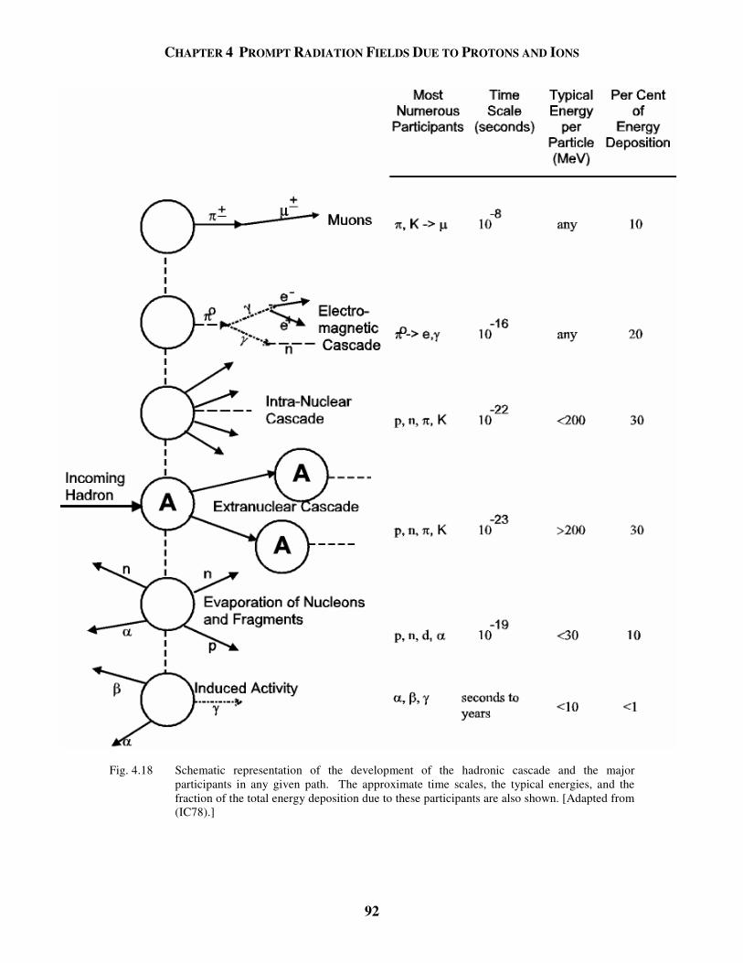
CHAPTER 4 PROMPT RADIATION FIELDS DUE TO PROTONS AND IONS
92
Fig. 4.18 Schematic representation of the development of the hadronic cascade and the major
participants in any given path. The approximate time scales, the typical energies, and the fraction of the total energy deposition due to these participants are also shown. [Adapted from (IC78).]
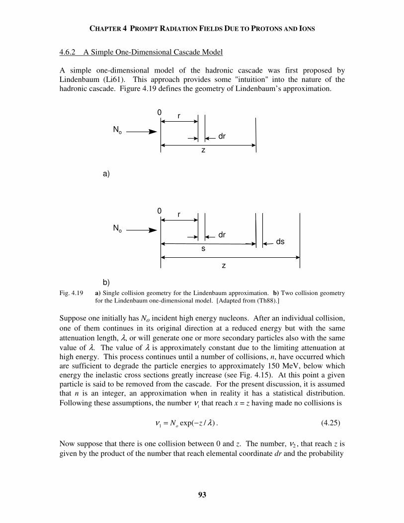
CHAPTER 4 PROMPT RADIATION FIELDS DUE TO PROTONS AND IONS
93
4.6.2 A Simple One-Dimensional Cascade Model A simple one-dimensional model of the hadronic cascade was first proposed by Lindenbaum (Li61). This approach provides some "intuition" into the nature of the hadronic cascade. Figure 4.19 defines the geometry of Lindenbaum’s approximation.
a)
b)
z
0
No
r
dr
s
0
No
r
drds
z
Fig. 4.19 a) Single collision geometry for the Lindenbaum approximation. b) Two collision geometry
for the Lindenbaum one-dimensional model. [Adapted from (Th88).] Suppose one initially has No incident high energy nucleons. After an individual collision, one of them continues in its original direction at a reduced energy but with the same attenuation length, λ, or will generate one or more secondary particles also with the same value of λ. The value of λ is approximately constant due to the limiting attenuation at high energy. This process continues until a number of collisions, n, have occurred which are sufficient to degrade the particle energies to approximately 150 MeV, below which energy the inelastic cross sections greatly increase (see Fig. 4.15). At this point a given particle is said to be removed from the cascade. For the present discussion, it is assumed that n is an integer, an approximation when in reality it has a statistical distribution. Following these assumptions, the number ν1 that reach x = z having made no collisions is 1 exp( / )oN zν λ= − . (4.25) Now suppose that there is one collision between 0 and z. The number, ν2 , that reach z is given by the product of the number that reach elemental coordinate dr and the probability
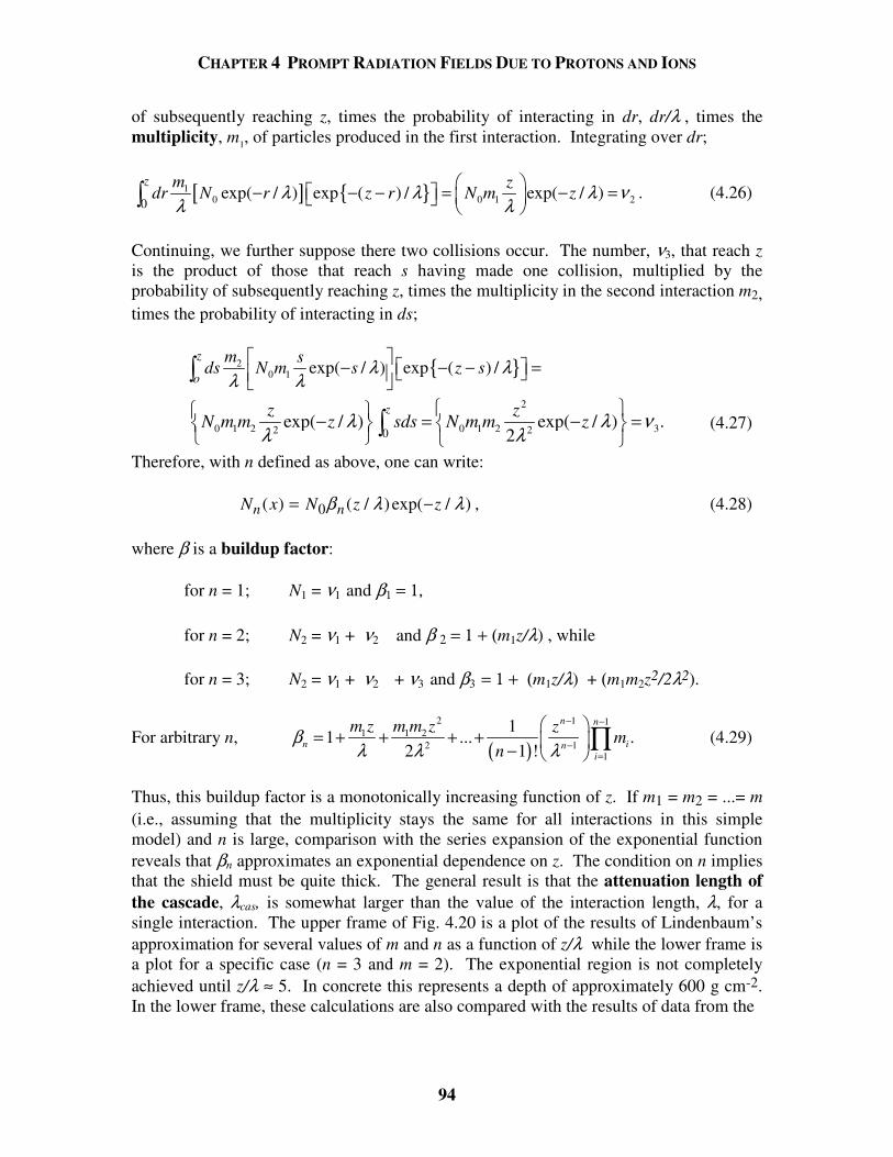
CHAPTER 4 PROMPT RADIATION FIELDS DUE TO PROTONS AND IONS
94
of subsequently reaching z, times the probability of interacting in dr, dr/λ , times the multiplicity, m1, of particles produced in the first interaction. Integrating over dr;
[ ] 10 0 1 20
exp( / ) exp ( ) / exp( / )z m zdr N r z r N m zλ λ λ ν
λ λ − − − = − =
. (4.26)
Continuing, we further suppose there two collisions occur. The number, ν3, that reach z is the product of those that reach s having made one collision, multiplied by the probability of subsequently reaching z, times the multiplicity in the second interaction m2, times the probability of interacting in ds;
2
0 1 exp( / ) exp ( ) /z
o
m sds N m s z sλ λ
λ λ − − − =
2
0 1 2 0 1 2 32 20exp( / ) exp( / ) .
2
zz zN m m z sds N m m zλ λ ν
λ λ − = − =
(4.27)
Therefore, with n defined as above, one can write:
N x N z zn n( ) ( / ) exp( / )= −0β λ λ , (4.28) where β is a buildup factor: for n = 1; N1 = ν1 and β1 = 1, for n = 2; N2 = ν1 + ν2 and β 2 = 1 + (m1z/λ) , while for n = 3; N2 = ν1 + ν2 + ν3 and β3 = 1 + (m1z/λ) + (m1m2z2/2λ2).
For arbitrary n, ( )2 1 1
1 1 22 1
1
11 ... .
2 1 !
n n
n ini
m z m m z zm
nβ
λ λ λ
− −
−=
= + + + + −
∏ (4.29)
Thus, this buildup factor is a monotonically increasing function of z. If m1 = m2 = ...= m (i.e., assuming that the multiplicity stays the same for all interactions in this simple model) and n is large, comparison with the series expansion of the exponential function reveals that βn approximates an exponential dependence on z. The condition on n implies that the shield must be quite thick. The general result is that the attenuation length of the cascade, λcas, is somewhat larger than the value of the interaction length, λ, for a single interaction. The upper frame of Fig. 4.20 is a plot of the results of Lindenbaum’s approximation for several values of m and n as a function of z/λ while the lower frame is a plot for a specific case (n = 3 and m = 2). The exponential region is not completely achieved until z/λ ≈ 5. In concrete this represents a depth of approximately 600 g cm-2. In the lower frame, these calculations are also compared with the results of data from the
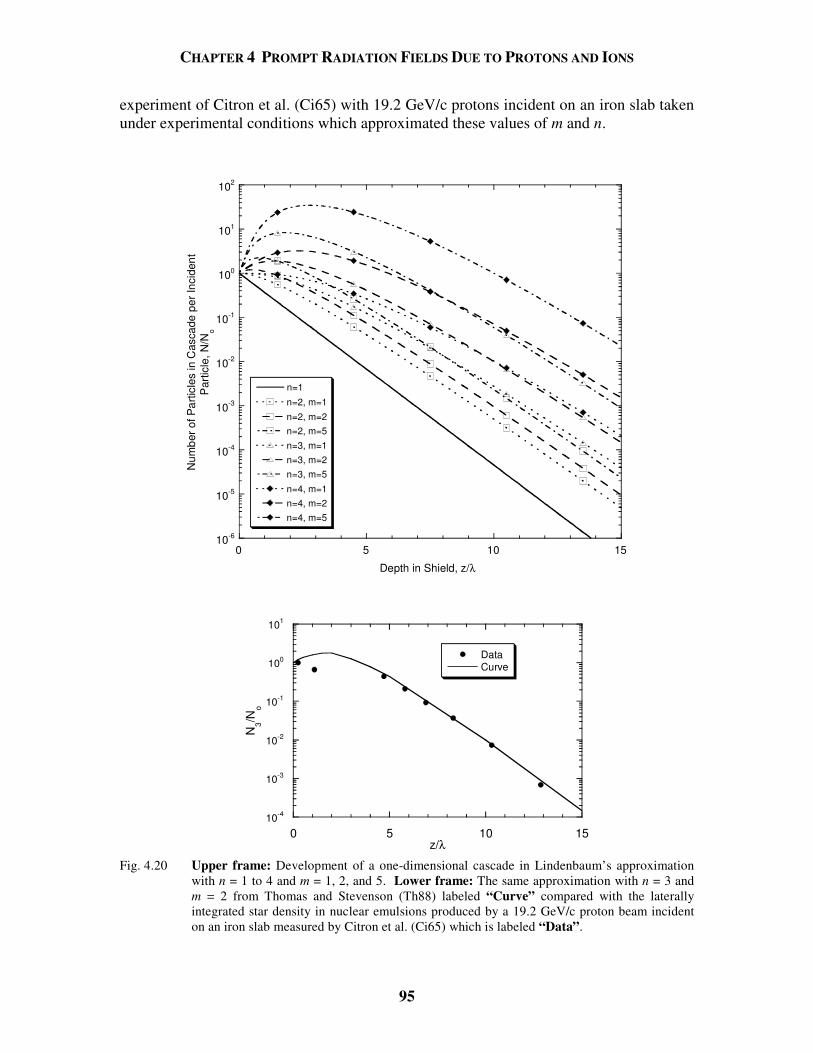
CHAPTER 4 PROMPT RADIATION FIELDS DUE TO PROTONS AND IONS
95
experiment of Citron et al. (Ci65) with 19.2 GeV/c protons incident on an iron slab taken under experimental conditions which approximated these values of m and n.
10-6
10-5
10-4
10-3
10-2
10-1
100
101
102
0 5 10 15
n=1
n=2, m=1
n=2, m=2n=2, m=5n=3, m=1n=3, m=2n=3, m=5
n=4, m=1n=4, m=2n=4, m=5
Num
ber o
f Par
ticle
s in
Cas
cade
per
Inci
dent
Par
ticle
, N/N
o
Depth in Shield, z/λ
10-4
10-3
10-2
10-1
100
101
0 5 10 15
DataCurve
N3/N
o
z/λ Fig. 4.20 Upper frame: Development of a one-dimensional cascade in Lindenbaum’s approximation
with n = 1 to 4 and m = 1, 2, and 5. Lower frame: The same approximation with n = 3 and m = 2 from Thomas and Stevenson (Th88) labeled “Curve” compared with the laterally integrated star density in nuclear emulsions produced by a 19.2 GeV/c proton beam incident on an iron slab measured by Citron et al. (Ci65) which is labeled “Data”.
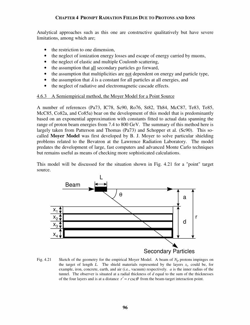
CHAPTER 4 PROMPT RADIATION FIELDS DUE TO PROTONS AND IONS
96
Analytical approaches such as this one are constructive qualitatively but have severe limitations, among which are;
• the restriction to one dimension, • the neglect of ionization energy losses and escape of energy carried by muons, • the neglect of elastic and multiple Coulomb scattering, • the assumption that all secondary particles go forward, • the assumption that multiplicities are not dependent on energy and particle type, • the assumption that λ is a constant for all particles at all energies, and • the neglect of radiative and electromagnetic cascade effects.
4.6.3 A Semiempirical method, the Moyer Model for a Point Source A number of references (Pa73, IC78, Sc90, Ro76, St82, Th84, McC87, Te83, Te85, McC85, Co82a, and Co85a) bear on the development of this model that is predominantly based on an exponential approximation with constants fitted to actual data spanning the range of proton beam energies from 7.4 to 800 GeV. The summary of this method here is largely taken from Patterson and Thomas (Pa73) and Schopper et al. (Sc90). This so-called Moyer Model was first developed by B. J. Moyer to solve particular shielding problems related to the Bevatron at the Lawrence Radiation Laboratory. The model predates the development of large, fast computers and advanced Monte Carlo techniques but remains useful as means of checking more sophisticated calculations. This model will be discussed for the situation shown in Fig. 4.21 for a "point" target source.
Beam
a
d
θ
r
L
x1
x2
x3
x4
Secondary Particles
Fig. 4.21 Sketch of the geometry for the empirical Moyer Model. A beam of Np protons impinges on the target of length L. The shield materials represented by the layers xi, could be, for example, iron, concrete, earth, and air (i.e., vacuum) respectively. a is the inner radius of the tunnel. The observer is situated at a radial thickness of d equal to the sum of the thicknesses of the four layers and is at a distance cscr r θ′ = from the beam-target interaction point.
CHAPTER 4 PROMPT RADIATION FIELDS DUE TO PROTONS AND IONS
97
The number of neutrons, dN/dE, which are emitted into a given element of solid angle dΩ at angle θ relative to a target struck by Np protons in an energy interval E + dE is given for a single shield material of thickness d by
2 csc
( ) exp( )p
dN d Y dN B E d
dE dEd Eθ
λ
= Ω − Ω , (4.30)
where B(E) is a buildup factor and the exponential function accounts for the attenuation of the radiation field by shielding of thickness, d, at the angle θ. The energy-dependent interaction length is denoted by λ(E). The role of the double differential of the yield is obvious. In the above, the flux density at coordinates (r,θ ) can be obtained at distance r′ from the target by including the factor
22222
1
csc
1
csc)(
1
rrdadAd
′==
+=Ω
θθ. (4.31)
The total fluence, Φ, at the point where the ray emerges from the shield is given by
max
min
2
2csc
( ) exp( )
E
E
pN d Y ddE B E
dEd Er
θλ
Φ = − Ω′
. (4.32)
The following are Moyer’s simplifying assumptions: A. λ(E) = λ = constant for E > 150 MeV and λ(E) = 0 for E < 150 MeV. This is a
simplified rendering of the leveling-off of the inelastic cross section at high energy. Thus,
max150MeV
2
2csc
( 150 MeV) exp - ( )Ep
nN d d Y
E dE B EdEdr
θλ
Φ > = Ω ′ . (4.33)
B. The neutrons emitted at angle θ can be represented by a simple function f (θ )
multiplied by a multiplicity factor M(Emax) that depends only on the incident energy, thus;
max2csc
( 150 MeV) exp - ( ) ( )pn
N dE M E f
r
θ θλ
Φ > = = ′
max2csc
exp - ( , )pN dg E
r
θ θλ
′
(4.34)
where g(Emax,θ ) is an angular distribution function that is constant for a given
value of Emax and for a particular target.
CHAPTER 4 PROMPT RADIATION FIELDS DUE TO PROTONS AND IONS
98
C. The dose equivalent per fluence, P, for neutrons is not strongly dependent on energy over a rather wide energy range near E ≈ 150 MeV (see Fig. 1.5). Thus the dose equivalent just outside of the shield due to neutrons with E > 150 MeV can be taken to be H150 ≈ P150 Φ (En > 150 MeV), where P150 is the value of this conversion factor at 150 MeV.
The total dose equivalent, H, is then given by H = kH150 where k > 1. (4.35) This implicitly assumes that the low-energy neutrons are in equilibrium with those having E > 150 MeV so that the spectrum no longer changes with depth. This is a valid assumption for a shield more than a few mean free paths thick. Thus, Moyer's assumptions lead to
( )150 max
2 2
( , ) cscexp
cscpkP N g E d
Ha d
θ θλθ
= − +
. (4.36)
One can generalize the results for the geometry shown in Fig. 4.21 with multiple materials in the shield. The parameter ζ, which replaces the ratio d/λ in the argument of the exponential function in Eq. (4.36), is introduced to take care of the n shielding components;
ζλι
==
xi
i
n
1, (4.37)
where the sum is over the n layers of shielding. Moyer model parameters have been determined by experiment. Stevenson (St82) and Thomas and Thomas (Th84) have determined from global fits to data over a wide domain of energy that f (θ ) is well described by ( ) exp( )f θ βθ= − , (4.38) where θ is in radians, β is in radians-1, and, in fact, β ≈ 2.3 rad-1 (for En > 150 MeV) for proton kinetic energies above a few GeV. Thus,
( )
( )2
( ) exp( )exp csc
csco pH E
Hr
βθ ζ θθ
− −= (4.39)
in which 1
n
ii
r a x=
= + (4.40)

CHAPTER 4 PROMPT RADIATION FIELDS DUE TO PROTONS AND IONS
99
and where the value of Ho(Ep)exp(-βθ) is determined from the yield data and empirical measurements. Ηο(Εp) is best fit as a power law; Ηο(Εp) = kEn. From such results, per incident proton;
Ho(Ep) = [(2.84 + 0.14) x 10-13] Ep(0.80 + 0.10) (Sv m2)
= 2.84 x 10⁻⁸ Ep0.8 (mrem m2) = 2.8 x 10⁻⁴ Ep0.8 (mrem cm2), (4.41)
with Ep in GeV. These results are derived for relatively "thick" targets (like accelerator magnets) in tunnel configurations. Schopper et al. (Sc90), based on Monte Carlo results gave values for "thin" targets of k = 2.0 x 10⁻¹⁴ (Sv m2) and n = 0.5. A thin-walled beam pipe would be an example of a "thin" target. The variations thus reflect buildup in the shower. For thick lateral shields close to the beam where the cascade immediately becomes fully developed and self-shielding arises, k = (6.9 + 0.1) x 10-15 (Sv m2) and n = 0.8 independent of target material (Sc90 and St87). The value of n = 0.8 for thick shields has also been verified by Torres (To96) and rigorously discussed by Gabriel et al. (Ga94). Similarly, recommended values of λ for concrete and other materials as a function of mass number A are; concrete: 1170 + 20 kg m-2 = 117 g cm-2
others: 428A 1/3 kg m-2 = 42.8A1/3 g cm-2. These values are 15-30% larger than the high energy nuclear interaction lengths (Table 1.2), a result consistent with that of Lindenbaum’s approximation concerning the values of λcas relative to those of λ. If one sets the partial derivative, /H θ∂ ∂ , equal to zero, one can derive an equation for determining the value of θ = θ ′ at which the maximum dose equivalent occurs; 0=′′+′−′ θθθβθζ sincos2sincos 2 . (4.42) Generally this equation can be solved by successive approximation methods. One can substitute into the above equation to get the maximum dose equivalent at a given radial depth. According to McCaslin (McC87), with r in meters and over a wide range of values of ζ, the following holds:
( )2
245.08.014
max exp1066.1r
EH pζζ−×= − (Sv per incident proton). (4.43)
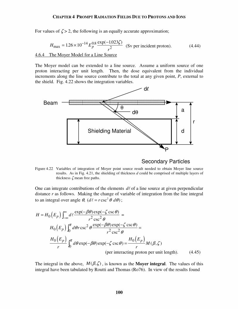
CHAPTER 4 PROMPT RADIATION FIELDS DUE TO PROTONS AND IONS
100
For values of ζ > 2, the following is an equally accurate approximation;
H Er
pmax..
exp( . )= × −−126 10102314 0 82
ζ (Sv per incident proton). (4.44)
4.6.4 The Moyer Model for a Line Source The Moyer model can be extended to a line source. Assume a uniform source of one proton interacting per unit length. Then, the dose equivalent from the individual increments along the line source contribute to the total at any given point, P, external to the shield. Fig. 4.22 shows the integration variables.
Beama
d
θ
r
Secondary Particles
Shielding Material
P
dθ
d
Figure 4.22 Variables of integration of Moyer point source result needed to obtain Moyer line source
results. As in Fig. 4.21, the shielding of thickness d could be comprised of multiple layers of thickness ζ mean free paths.
One can integrate contributions of the elements d of a line source at given perpendicular distance r as follows. Making the change of variable of integration from the line integral to an integral over angle θ, 2( csc )d r dθ θ= ;
( )0 2 2exp( )exp( csc )
cscpH H E d
r
βθ ζ θθ
∞−∞
− −= =
( ) 20 2 20
exp( ) exp( csc )csc
cscpH E d r
r
π βθ ζ θθ θθ
− − =
( ) ( )0 0
0exp( ) exp( csc ) ( , )
p pH E H Ed M
r rπ
θ βθ ζ θ β ζ− − =
(per interacting proton per unit length). (4.45) The integral in the above, M ( , )β ζ , is known as the Moyer integral. The values of this integral have been tabulated by Routti and Thomas (Ro76). In view of the results found
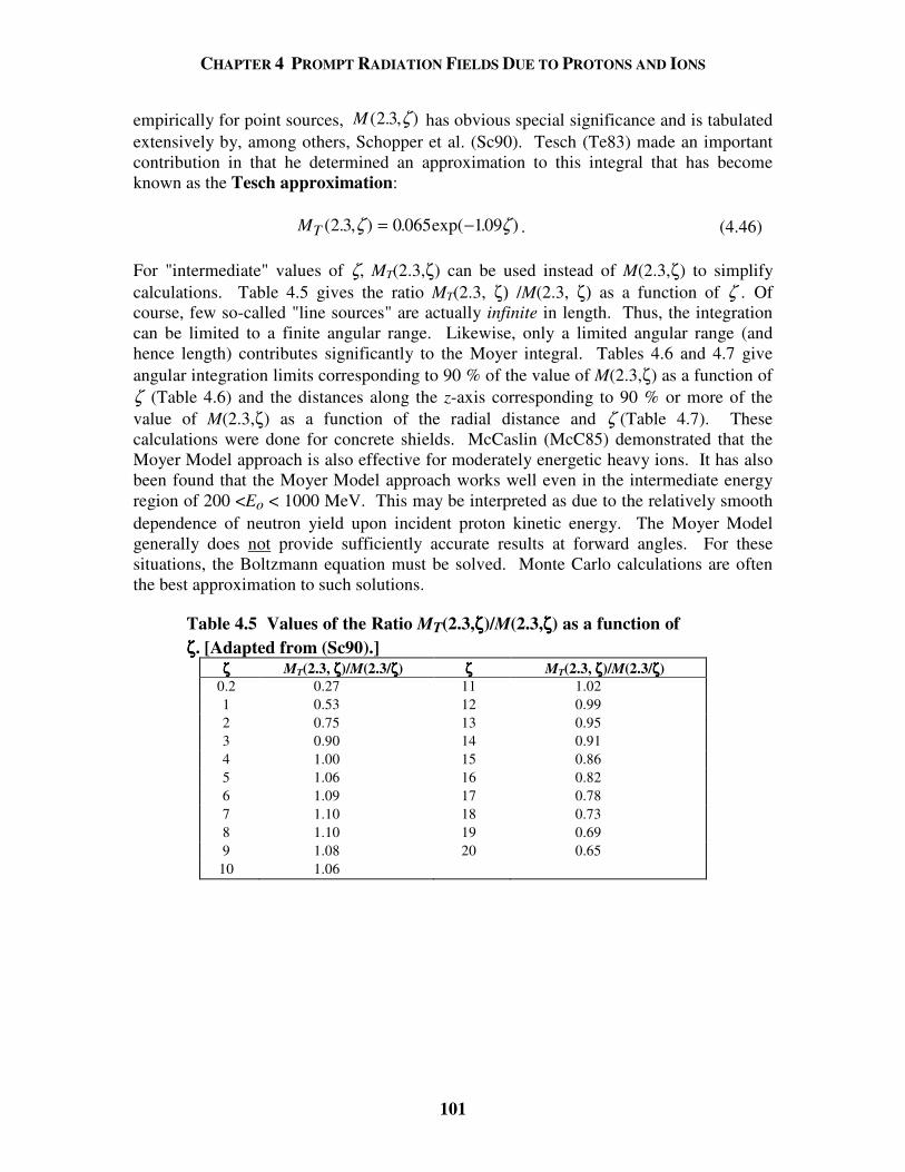
CHAPTER 4 PROMPT RADIATION FIELDS DUE TO PROTONS AND IONS
101
empirically for point sources, M ( . , )2 3 ζ has obvious special significance and is tabulated extensively by, among others, Schopper et al. (Sc90). Tesch (Te83) made an important contribution in that he determined an approximation to this integral that has become known as the Tesch approximation: MT ( . , ) . exp( . )2 3 0 065 109ζ ζ= − . (4.46) For "intermediate" values of ζ, MT(2.3,ζ) can be used instead of M(2.3,ζ) to simplify calculations. Table 4.5 gives the ratio MT(2.3, ζ) /M(2.3, ζ) as a function of ζ . Of course, few so-called "line sources" are actually infinite in length. Thus, the integration can be limited to a finite angular range. Likewise, only a limited angular range (and hence length) contributes significantly to the Moyer integral. Tables 4.6 and 4.7 give angular integration limits corresponding to 90 % of the value of M(2.3,ζ) as a function of ζ (Table 4.6) and the distances along the z-axis corresponding to 90 % or more of the value of M(2.3,ζ) as a function of the radial distance and ζ (Table 4.7). These calculations were done for concrete shields. McCaslin (McC85) demonstrated that the Moyer Model approach is also effective for moderately energetic heavy ions. It has also been found that the Moyer Model approach works well even in the intermediate energy region of 200 <Eo < 1000 MeV. This may be interpreted as due to the relatively smooth dependence of neutron yield upon incident proton kinetic energy. The Moyer Model generally does not provide sufficiently accurate results at forward angles. For these situations, the Boltzmann equation must be solved. Monte Carlo calculations are often the best approximation to such solutions.
Table 4.5 Values of the Ratio MT(2.3,ζζζζ)/M(2.3,ζζζζ) as a function of ζζζζ. [Adapted from (Sc90).]
ζζζζ MT(2.3, ζζζζ)/M(2.3/ζζζζ) ζζζζ MT(2.3, ζζζζ)/M(2.3/ζζζζ) 0.2 0.27 11 1.02 1 0.53 12 0.99 2 0.75 13 0.95 3 0.90 14 0.91 4 1.00 15 0.86 5 1.06 16 0.82 6 1.09 17 0.78 7 1.10 18 0.73 8 1.10 19 0.69 9 1.08 20 0.65
10 1.06
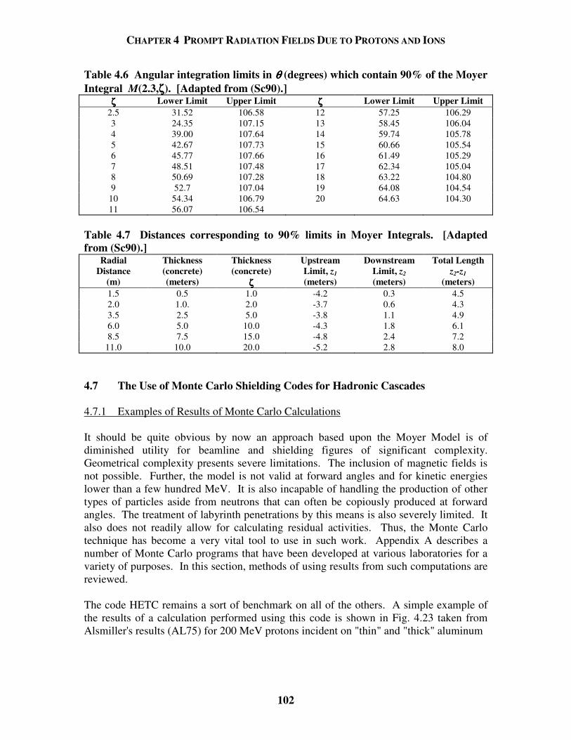
CHAPTER 4 PROMPT RADIATION FIELDS DUE TO PROTONS AND IONS
102
Table 4.6 Angular integration limits in θθθθ (degrees) which contain 90% of the Moyer Integral M(2.3,ζζζζ). [Adapted from (Sc90).]
ζζζζ Lower Limit Upper Limit ζζζζ Lower Limit Upper Limit 2.5 31.52 106.58 12 57.25 106.29 3 24.35 107.15 13 58.45 106.04 4 39.00 107.64 14 59.74 105.78 5 42.67 107.73 15 60.66 105.54 6 45.77 107.66 16 61.49 105.29 7 48.51 107.48 17 62.34 105.04 8 50.69 107.28 18 63.22 104.80 9 52.7 107.04 19 64.08 104.54
10 54.34 106.79 20 64.63 104.30 11 56.07 106.54
Table 4.7 Distances corresponding to 90% limits in Moyer Integrals. [Adapted from (Sc90).]
Radial Distance
(m)
Thickness (concrete) (meters)
Thickness (concrete)
ζζζζ
Upstream Limit, z1 (meters)
Downstream Limit, z2 (meters)
Total Length z2-z1
(meters) 1.5 0.5 1.0 -4.2 0.3 4.5 2.0 1.0. 2.0 -3.7 0.6 4.3 3.5 2.5 5.0 -3.8 1.1 4.9 6.0 5.0 10.0 -4.3 1.8 6.1 8.5 7.5 15.0 -4.8 2.4 7.2
11.0 10.0 20.0 -5.2 2.8 8.0 4.7 The Use of Monte Carlo Shielding Codes for Hadronic Cascades 4.7.1 Examples of Results of Monte Carlo Calculations It should be quite obvious by now an approach based upon the Moyer Model is of diminished utility for beamline and shielding figures of significant complexity. Geometrical complexity presents severe limitations. The inclusion of magnetic fields is not possible. Further, the model is not valid at forward angles and for kinetic energies lower than a few hundred MeV. It is also incapable of handling the production of other types of particles aside from neutrons that can often be copiously produced at forward angles. The treatment of labyrinth penetrations by this means is also severely limited. It also does not readily allow for calculating residual activities. Thus, the Monte Carlo technique has become a very vital tool to use in such work. Appendix A describes a number of Monte Carlo programs that have been developed at various laboratories for a variety of purposes. In this section, methods of using results from such computations are reviewed. The code HETC remains a sort of benchmark on all of the others. A simple example of the results of a calculation performed using this code is shown in Fig. 4.23 taken from Alsmiller's results (AL75) for 200 MeV protons incident on "thin" and "thick" aluminum
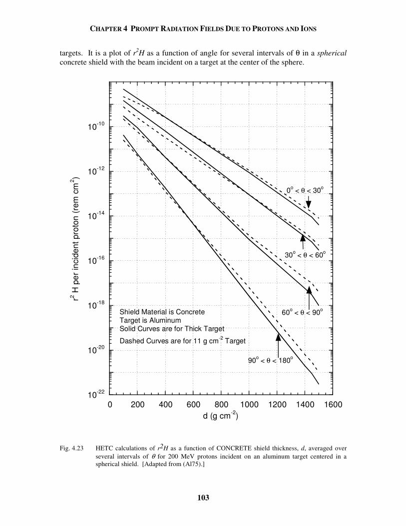
CHAPTER 4 PROMPT RADIATION FIELDS DUE TO PROTONS AND IONS
103
targets. It is a plot of r2H as a function of angle for several intervals of θ in a spherical concrete shield with the beam incident on a target at the center of the sphere.
10-22
10-20
10-18
10-16
10-14
10-12
10-10
0 200 400 600 800 1000 1200 1400 1600
r2 H p
er in
cide
nt p
roto
n (r
em c
m2 )
d (g cm-2)
0o < θ < 30o
30o < θ < 60o
60o < θ < 90o
90o < θ < 180o
Shield Material is ConcreteTarget is AluminumSolid Curves are for Thick Target
Dashed Curves are for 11 g cm-2 Target
Fig. 4.23 HETC calculations of r2H as a function of CONCRETE shield thickness, d, averaged over
several intervals of θ for 200 MeV protons incident on an aluminum target centered in a spherical shield. [Adapted from (Al75).]
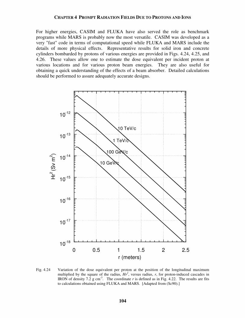
CHAPTER 4 PROMPT RADIATION FIELDS DUE TO PROTONS AND IONS
104
For higher energies, CASIM and FLUKA have also served the role as benchmark programs while MARS is probably now the most versatile. CASIM was developed as a very "fast" code in terms of computational speed while FLUKA and MARS include the details of more physical effects. Representative results for solid iron and concrete cylinders bombarded by protons of various energies are provided in Figs. 4.24, 4.25, and 4.26. These values allow one to estimate the dose equivalent per incident proton at various locations and for various proton beam energies. They are also useful for obtaining a quick understanding of the effects of a beam absorber. Detailed calculations should be performed to assure adequately accurate designs.
10-18
10-17
10-16
10-15
10-14
10-13
10-12
0 0.5 1 1.5 2 2.5
Hr2
(Sv
m2 )
r (meters)
10 TeV/c
1 TeV/c
100 GeV/c
10 GeV/c
Fig. 4.24 Variation of the dose equivalent per proton at the position of the longitudinal maximum
multiplied by the square of the radius, Hr2, versus radius, r, for proton-induced cascades in IRON of density 7.2 g cm-3. The coordinate r is defined as in Fig. 4.22. The results are fits to calculations obtained using FLUKA and MARS. [Adapted from (Sc90).]
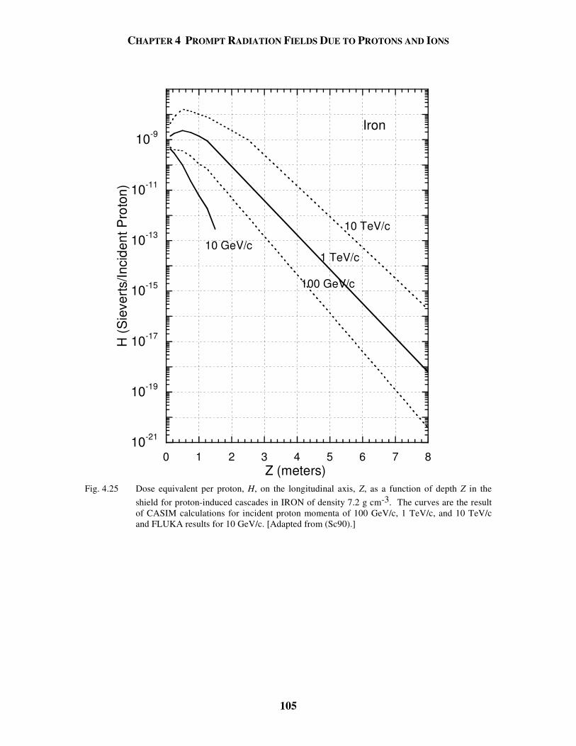
CHAPTER 4 PROMPT RADIATION FIELDS DUE TO PROTONS AND IONS
105
10-21
10-19
10-17
10-15
10-13
10-11
10-9
0 1 2 3 4 5 6 7 8
H (
Sie
verts
/Inci
dent
Pro
ton)
Z (meters)
10 GeV/c
10 TeV/c
1 TeV/c
100 GeV/c
Iron
Fig. 4.25 Dose equivalent per proton, H, on the longitudinal axis, Z, as a function of depth Z in the
shield for proton-induced cascades in IRON of density 7.2 g cm-3. The curves are the result of CASIM calculations for incident proton momenta of 100 GeV/c, 1 TeV/c, and 10 TeV/c and FLUKA results for 10 GeV/c. [Adapted from (Sc90).]
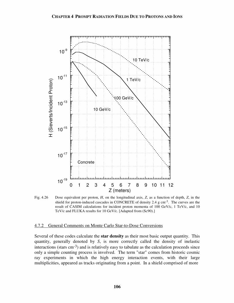
CHAPTER 4 PROMPT RADIATION FIELDS DUE TO PROTONS AND IONS
106
10-19
10-17
10-15
10-13
10-11
10-9
0 1 2 3 4 5 6 7 8 9 10 11 12
H (
Sie
verts
/Inci
dent
Pro
ton)
Z (meters)
10 TeV/c
1 TeV/c
100 GeV/c
10 GeV/c
Concrete
Fig. 4.26 Dose equivalent per proton, H, on the longitudinal axis, Z, as a function of depth, Z, in the
shield for proton-induced cascades in CONCRETE of density 2.4 g cm-3. The curves are the result of CASIM calculations for incident proton momenta of 100 GeV/c, 1 TeV/c, and 10 TeV/c and FLUKA results for 10 GeV/c. [Adapted from (Sc90).]
4.7.2 General Comments on Monte Carlo Star-to-Dose Conversions Several of these codes calculate the star density as their most basic output quantity. This quantity, generally denoted by S, is more correctly called the density of inelastic interactions (stars cm-3) and is relatively easy to tabulate as the calculation proceeds since only a simple counting process is involved. The term "star" comes from historic cosmic ray experiments in which the high energy interaction events, with their large multiplicities, appeared as tracks originating from a point. In a shield comprised of more
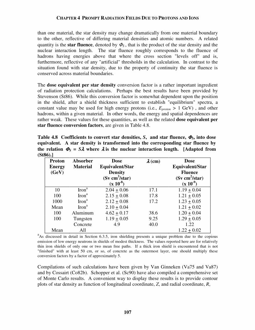
CHAPTER 4 PROMPT RADIATION FIELDS DUE TO PROTONS AND IONS
107
than one material, the star density may change dramatically from one material boundary to the other, reflective of differing material densities and atomic numbers. A related quantity is the star fluence, denoted by ΦS , that is the product of the star density and the nuclear interaction length. The star fluence roughly corresponds to the fluence of hadrons having energies above that where the cross section "levels off" and is, furthermore, reflective of any "artificial" thresholds in the calculation. In contrast to the situation found with star density, due to the property of continuity the star fluence is conserved across material boundaries. The dose equivalent per star density conversion factor is a rather important ingredient of radiation protection calculations. Perhaps the best results have been provided by Stevenson (St86). While this conversion factor is somewhat dependent upon the position in the shield, after a shield thickness sufficient to establish "equilibrium" spectra, a constant value may be used for high energy protons (i.e., Eproton > 1 GeV) , and other hadrons, within a given material. In other words, the energy and spatial dependences are rather weak. These values for these quantities, as well as the related dose equivalent per star fluence conversion factors, are given in Table 4.8. Table 4.8 Coefficients to convert star densities, S, and star fluence, ΦΦΦΦS, into dose equivalent. A star density is transformed into the corresponding star fluence by the relation ΦΦΦΦS = Sλλλλ where λλλλ is the nuclear interaction length. [Adapted from (St86).]
Proton Energy (GeV)
Absorber Material
Dose Equivalent/Star
Density (Sv cm3/star)
(x 10-8)
λλλλ (cm) Dose Equivalent/Star
Fluence (Sv cm2/star)
(x 10-9) 10 Irona 2.04 + 0.06 17.1 1.19 + 0.04
100 Irona 2.15 + 0.08 17.8 1.21 + 0.05 1000 Irona 2.12 + 0.08 17.2 1.23 + 0.05 Mean Irona 2.10 + 0.04 1.21 + 0.02 100 Aluminum 4.62 + 0.17 38.6 1.20 + 0.04 100 Tungsten 1.19 + 0.05 9.25 1.29 + 0.05
Concrete 4.9 40.0 1.22 Mean All 1.22 + 0.02
aAs discussed in detail in Section 6.3.5, iron shielding presents a unique problem due to the copious emission of low energy neutrons in shields of modest thickness. The values reported here are for relatively thin iron shields of only one or two mean free paths. If a thick iron shield is encountered that is not "finished" with at least 50 cm, or so, of concrete as the outermost layer, one should multiply these conversion factors by a factor of approximately 5. Compilations of such calculations have been given by Van Ginneken (Va75 and Va87) and by Cossairt (Co82b). Schopper et al. (Sc90) have also compiled a comprehensive set of Monte Carlo results. A convenient way to display these results is to provide contour plots of star density as function of longitudinal coordinate, Z, and radial coordinate, R,
CHAPTER 4 PROMPT RADIATION FIELDS DUE TO PROTONS AND IONS
108
assuming cylindrical symmetry. Appendix C provides examples of the results of such hadronic Monte Carlo calculations that are meant to illustrate a number of situations commonly encountered. One of the salient advantages of the Monte Carlo method is the ability to handle configurations of arbitrary complexity and results for both solid cylinders and more complicated example configurations are provided in Appendix C. 4.7.3 Shielding Against Muons at Proton Accelerators The production of muons has been discussed previously in Section 4.2.4. At the higher energies, there are significant complications in that muon creation mechanisms, in addition to the production of pions and kaons and their subsequent decays, are possible. However, the muons from pion decay and kaon decay generally, but not universally, represent the most important consideration in practical shielding calculations. In Monte Carlo calculations, it is straightforward to "create" muons and follow them through the shielding medium. Muon transport is well understood, as discussed in the preceding chapters. The particle energy downgrades quickly in hadronic showers so the most penetrating muons must originate in the first few generations of the cascade process. These energetic muons are not distributed over a large volume of space as are the neutrons. However, geometric effects or deflections by magnetic fields encountered near the point of production can affect the muon fluence at large distances. Thus, the presence of large "empty" spaces, that is, decay paths (vacuum or air), near the point of interaction provide opportunity for the pions or kaons to decay into muons before they can be removed by nuclear interactions in solid materials. This is particularly important for the typical situation of a target used to produce secondary beams followed (downstream) by an air or vacuum gap (the space for decay into muons) and then a beam absorber. If magnetic fields are present, the muon fluence generally peaks in the bend plane. Multiple Coulomb scattering from nuclei is an important effect in muon transport. Generally the most copious sources of muons are those due to the decay of pions and kaons. There are several important facts about such muons that are summarized below: A. The decay length (mean length for π or K to decay), Λ, is given by Λπ = 55.9p (meters), where p is the pion momentum in GeV/c, and ΛΚ = 7.51p (meters), where p is the kaon momentum in GeV/c. The available decay path in conjunction with the decay length can be used to
estimate the total number of muons present. For example, a beam of 107 pions at 20 GeV/c will decay in a distance of 50 meters into 107 x [50 meters]/[(56 x 20) meters decay length] = 4.5 x 10⁵ muons. This uses the fact that the decay path (50 meters) is small compared with the mean decay length of 1120 meters. If the decay path, x, was comparable to the decay length, Λ, the final intensity would need to be multiplied by the exponential factor 1 - exp(x/Λ).
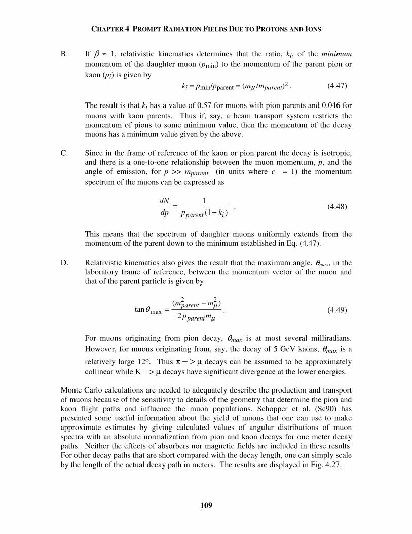
CHAPTER 4 PROMPT RADIATION FIELDS DUE TO PROTONS AND IONS
109
B. If β ≈ 1, relativistic kinematics determines that the ratio, ki, of the minimum momentum of the daughter muon (pmin) to the momentum of the parent pion or kaon (pi) is given by
ki = pmin/pparent = (mµ /mparent)2 . (4.47) The result is that ki has a value of 0.57 for muons with pion parents and 0.046 for
muons with kaon parents. Thus if, say, a beam transport system restricts the momentum of pions to some minimum value, then the momentum of the decay muons has a minimum value given by the above.
C. Since in the frame of reference of the kaon or pion parent the decay is isotropic,
and there is a one-to-one relationship between the muon momentum, p, and the angle of emission, for p >> mparent (in units where c = 1) the momentum spectrum of the muons can be expressed as
dNdp p kparent i
=−
11( )
. (4.48)
This means that the spectrum of daughter muons uniformly extends from the
momentum of the parent down to the minimum established in Eq. (4.47). D. Relativistic kinematics also gives the result that the maximum angle, θmax, in the
laboratory frame of reference, between the momentum vector of the muon and that of the parent particle is given by
tan( )
maxθ µ
µ=
−m m
p mparent
parent
2 2
2. (4.49)
For muons originating from pion decay, θmax is at most several milliradians.
However, for muons originating from, say, the decay of 5 GeV kaons, θmax is a
relatively large 12o. Thus π − > µ decays can be assumed to be approximately collinear while K − > µ decays have significant divergence at the lower energies.
Monte Carlo calculations are needed to adequately describe the production and transport of muons because of the sensitivity to details of the geometry that determine the pion and kaon flight paths and influence the muon populations. Schopper et al, (Sc90) has presented some useful information about the yield of muons that one can use to make approximate estimates by giving calculated values of angular distributions of muon spectra with an absolute normalization from pion and kaon decays for one meter decay paths. Neither the effects of absorbers nor magnetic fields are included in these results. For other decay paths that are short compared with the decay length, one can simply scale by the length of the actual decay path in meters. The results are displayed in Fig. 4.27.
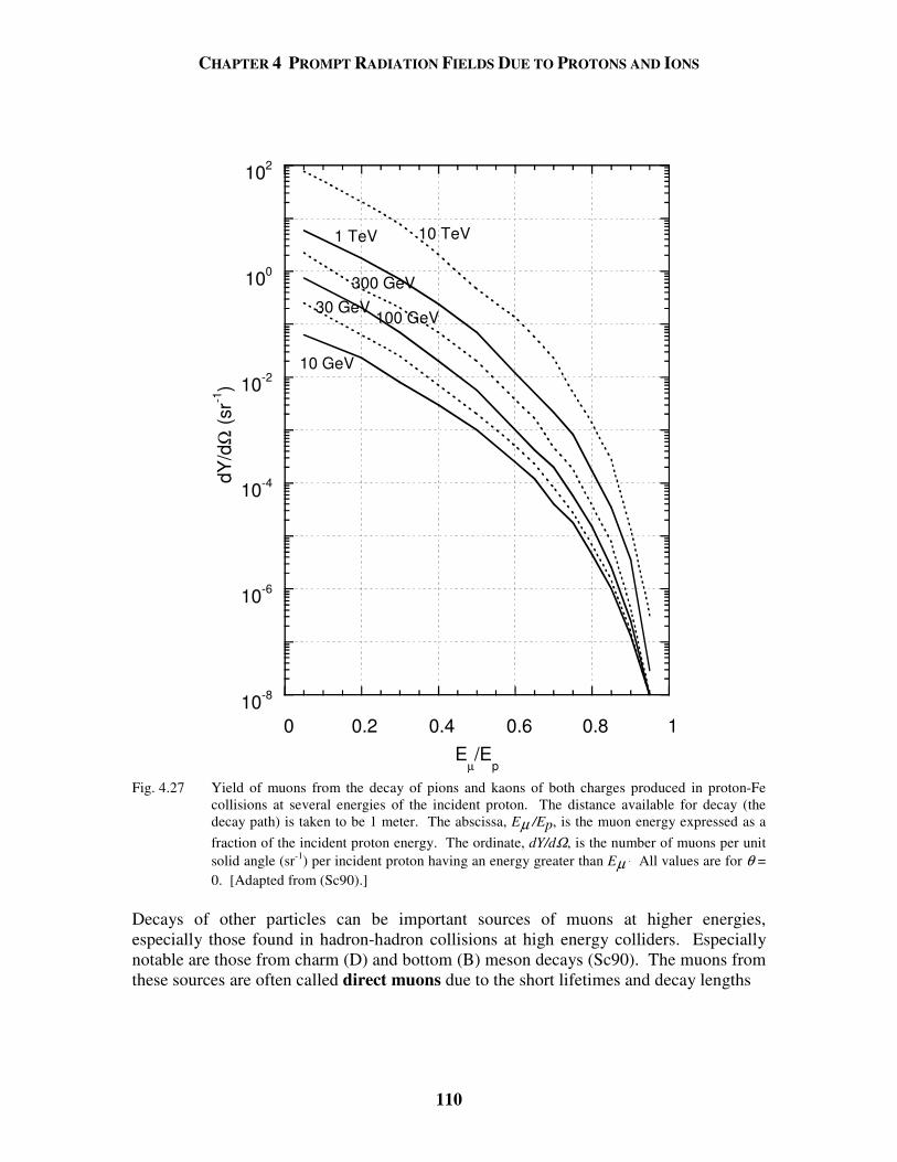
CHAPTER 4 PROMPT RADIATION FIELDS DUE TO PROTONS AND IONS
110
10-8
10-6
10-4
10-2
100
102
0 0.2 0.4 0.6 0.8 1
dY/d
Ω (s
r-1)
Eµ/E
p
10 TeV1 TeV
300 GeV
100 GeV30 GeV
10 GeV
Fig. 4.27 Yield of muons from the decay of pions and kaons of both charges produced in proton-Fe
collisions at several energies of the incident proton. The distance available for decay (the decay path) is taken to be 1 meter. The abscissa, Eµ /Ep, is the muon energy expressed as a fraction of the incident proton energy. The ordinate, dY/dΩ, is the number of muons per unit solid angle (sr-1) per incident proton having an energy greater than Eµ . All values are for θ = 0. [Adapted from (Sc90).]
Decays of other particles can be important sources of muons at higher energies, especially those found in hadron-hadron collisions at high energy colliders. Especially notable are those from charm (D) and bottom (B) meson decays (Sc90). The muons from these sources are often called direct muons due to the short lifetimes and decay lengths
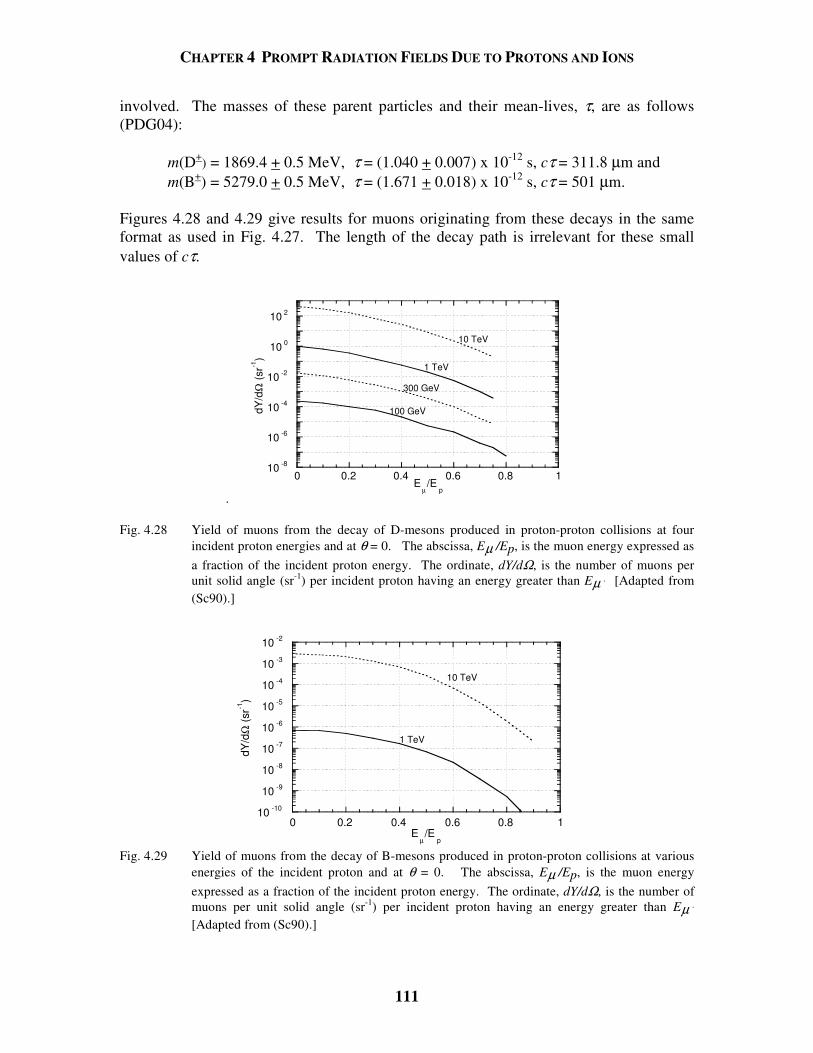
CHAPTER 4 PROMPT RADIATION FIELDS DUE TO PROTONS AND IONS
111
involved. The masses of these parent particles and their mean-lives, τ, are as follows (PDG04):
m(D+) = 1869.4 + 0.5 MeV, τ = (1.040 + 0.007) x 10-12 s, cτ = 311.8 µm and m(B+) = 5279.0 + 0.5 MeV, τ = (1.671 + 0.018) x 10-12 s, cτ = 501 µm.
Figures 4.28 and 4.29 give results for muons originating from these decays in the same format as used in Fig. 4.27. The length of the decay path is irrelevant for these small values of cτ.
.
10 -8
10 -6
10 -4
10 -2
10 0
10 2
0 0.2 0.4 0.6 0.8 1
dY/d
Ω (s
r-1)
Eµ/E
p
10 TeV
1 TeV
300 GeV
100 GeV
Fig. 4.28 Yield of muons from the decay of D-mesons produced in proton-proton collisions at four incident proton energies and at θ = 0. The abscissa, Eµ /Ep, is the muon energy expressed as a fraction of the incident proton energy. The ordinate, dY/dΩ, is the number of muons per unit solid angle (sr-1) per incident proton having an energy greater than Eµ . [Adapted from (Sc90).]
10 -10
10 -9
10 -8
10 -7
10 -6
10 -5
10 -4
10 -3
10 -2
0 0.2 0.4 0.6 0.8 1
dY/d
Ω (s
r-1)
Eµ/E
p
10 TeV
1 TeV
Fig. 4.29 Yield of muons from the decay of B-mesons produced in proton-proton collisions at various
energies of the incident proton and at θ = 0. The abscissa, Eµ /Ep, is the muon energy expressed as a fraction of the incident proton energy. The ordinate, dY/dΩ, is the number of muons per unit solid angle (sr-1) per incident proton having an energy greater than Eµ . [Adapted from (Sc90).]
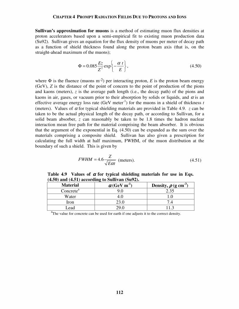
CHAPTER 4 PROMPT RADIATION FIELDS DUE TO PROTONS AND IONS
112
Sullivan’s approximation for muons is a method of estimating muon flux densities at proton accelerators based upon a semi-empirical fit to existing muon production data (Su92). Sullivan gives an equation for the flux density of muons per meter of decay path as a function of shield thickness found along the proton beam axis (that is, on the straight-ahead maximum of the muons);
2
0.085 exp
Ez tZ E
α Φ = −
, (4.50)
where Φ is the fluence (muons m-2) per interacting proton, E is the proton beam energy (GeV), Z is the distance of the point of concern to the point of production of the pions and kaons (meters), z is the average path length (i.e., the decay path) of the pions and kaons in air, gases, or vacuum prior to their absorption by solids or liquids, and α is an effective average energy loss rate (GeV meter-1) for the muons in a shield of thickness t (meters). Values of α for typical shielding materials are provided in Table 4.9. z can be taken to be the actual physical length of the decay path, or according to Sullivan, for a solid beam absorber, z can reasonably be taken to be 1.8 times the hadron nuclear interaction mean free path for the material comprising the beam absorber. It is obvious that the argument of the exponential in Eq. (4.50) can be expanded as the sum over the materials comprising a composite shield. Sullivan has also given a prescription for calculating the full width at half maximum, FWHM, of the muon distribution at the boundary of such a shield. This is given by
4.6Z
FWHME tα
= (meters). (4.51)
Table 4.9 Values of αααα for typical shielding materials for use in Eqs. (4.50) and (4.51) according to Sullivan (Su92).
Material αααα (GeV m-1) Density, ρρρρ (g cm-3) Concretea 9.0 2.35
Water 4.0 1.0 Iron 23.0 7.4 Lead 29.0 11.3
aThe value for concrete can be used for earth if one adjusts it to the correct density.
CHAPTER 4 PROMPT RADIATION FIELDS DUE TO PROTONS AND IONS
113
Problems 1. One can use measurement results to check Sullivan’s formula, Eq. (4.4), for
hadron fluence above 40 MeV for high-energy proton interactions. Check the agreement for the 22 and 225 GeV/c data in Figs. 4.7 and 4.8 for 3 representative angles at one meter. (Ignore the fact that the formula is for hadrons > 40 MeV while the only data provided is for hadrons >35 MeV and > 50 MeV, but do not ignore the difference between normalizing to incident versus interacting protons.) (It is valid to make the comparison on yield per interacting proton since the results in Fig. 4.8 is for targets approximately 1 interaction length long.) Comment on the quality of the agreement.
2. Calculations can also be used to check the Tesch curve for dose equivalent at θ =
90o (Fig. 4.10). Use the 200 MeV calculations in Fig. 4.4 to do this by crudely numerically integrating the 60o < θ < 90o yields to determine the average energy of the neutrons and the total fluence at θ = 90o and at 1 meter. Use the results along with dose equivalent per fluence curves to obtain the dose equivalent per proton to compare with Tesch’s result. (Iron is considered equivalent to copper for this problem.)
3. A copper target at an accelerator is struck by 1 µA of 100 MeV protons.
a) Use Tesch’s curve in Fig. 4.10 to calculate the dose equivalent rate at 2 m and θ = 90o relative to this target.
b) Compare this result with the neutron dose equivalent rate calculated in Chapter 3,
Problem 5 for an electron accelerator having the same intensity and beam energy and discuss. (Scale the relevant result of Chapter 3, Problem 5 by the appropriate yield for copper versus tungsten.)
4. It is often necessary to work from fragmentary data to determine other quantities. a) Use McCaslin's results, Eqs. (4.13, 4.14, and 4.15), and the appropriate dose
equivalent/fluence to calculate the dose equivalent rate at 1 meter and at θ = 30o for a target struck by 108 670 MeV/amu 20Ne ions per sec. (Hint: Use all available spectrum information.)
b) Use McCaslin's results to obtain the total yield of neutrons per ion with En > 6.5
MeV. Assuming the target to be iron or copper, how does this yield correspond to that due to 700 MeV protons? Do this for both En > 6.5 MeV and En > 20 MeV to understand the overall composition. Hint: Integrate over the unit sphere (double integral over spherical coordinates θ & φ) and convert all quantities associated with angles from degrees to radians.
CHAPTER 4 PROMPT RADIATION FIELDS DUE TO PROTONS AND IONS
114
The following indefinite integrals are needed:
3 5 7sin
...3 3! 5 5! 7 7!
dx x x x xx
x= − + − +
⋅ ⋅ ⋅
[ ]
2 2
sin cossin
axax e a bx b bx
dxe bxa b
−=
+
The elemental area on the sphere of radius r is dA = r2 sin θ dθdφ, where φ is the standard azimuthal coordinate in a spherical coordinate system.
5. It is asserted that if the assumption is made that the limiting attenuation is simply
geometric, with the nucleon radius equal to 1.2 x 10⁻¹³ cm, then ρλatten = 36.7A1/3 (g cm-2). Show this to be the case using the volume of a nucleus and nucleons along with the cross section.
6. a) Use the Moyer Model to calculate the dose equivalent rate (mrem/hr) lateral (θ =
90o) to a magnet centered in a 1.5 m radius tunnel. The magnet is struck by 1012 protons at 100 GeV (per sec). The tunnel walls consist of 1/3 m concrete followed by soil having the same composition [ρ(concrete) = 2.5 g cm-3, ρ (soil) = 2.0 g cm-3]. Perform the same calculation for several thicknesses of soil out to 6 meters of soil radially. Do this for increments of 1 meter from 1 meter to 6 meters of soil.
b) Calculate the result if the same beam loss occurs uniformly over a string of such magnets 100 meters long in the same tunnel at the same soil thicknesses as above. Use the Tesch approximation. Approximately how many meters of beam loss does it take to cause 90% of the calculated dose equivalent rate at 6 m of lateral soil shield?
c) For the point loss in part a), at what value of θ does the maximum dose equivalent
rate occur and what is its magnitude outside of 6 meters of soil shield? (Use successive approximations to solve.)
7. An accelerator delivers 1012 1 TeV protons per second head-on on the inner edge
of a magnet. Use the CASIM calculations found in Appendix C to determine the approximate dose equivalent rate at R = 400 centimeters and compare with a result using the Moyer equation for point loss. Both calculations should be at the location of the maximum dose equivalent. Assume ρ (concrete) = 2.5 g cm-3 and ρ (soil) = 2.25 g cm-3. Why might there be an explainable disagreement between the two results?
CHAPTER 4 PROMPT RADIATION FIELDS DUE TO PROTONS AND IONS
115
8. Using the results of Monte Carlo hadron calculations (FLUKA/MARS), calculate, for solid shields of iron (cylinders), what longitudinal thickness of iron is needed to achieve the same hadron dose equivalent per proton on the beam axis as found at R = 50 cm at 10 GeV/c, 100 GeV/c, 1000 GeV/c and 10 TeV/c. Use the maximum value of H (r = 50 cm).
9. In Fig. 4.4, we have calculations of neutron energy spectra for 200 MeV protons
incident on various targets, including aluminum. In Fig. 4.23, calculations of dose equivalent values for spherical concrete shielding surrounding aluminum targets at Ep = 200 MeV are given. At shielding thicknesses approaching zero and at forward angles, are the two results in "sensible" (that is, approximate, agreement)? (Hint: "Integrate" crudely over the forward spectrum to obtain the fluence/proton and convert this fluence to dose equivalent.)
a) Make the comparison for zero shield thickness and in the angular range 0 < θ <
30o. b) Now use the shielding calculations to obtain the dose equivalent rate (rem h-1) due
to a 1 µA beam incident at 200 MeV on such a thick target at a distance of 4 m from the target with 0, 1, 2, & 3 m of intervening concrete shielding (ρ = 2.5
g cm-3) for θ = 15o and θ = 75o. (Hint: Use the center of the angular bins.) 10. Assume that a target is struck by 100 GeV protons and that a 10 m long decay
space exists for π and K decay. Use the curves in Fig. 4.27 to crudely estimate the muon flux density and dose equivalent rates (mrem/h) at 1 km away and at θ = 0o if 1012 protons/second are targeted in this manner if the following additional assumptions are made:
a) Assume that there is no shielding present and neglect air scattering and in-
scattering from the ground. (Hint: The muon yield for this decay space will scale with the length of the decay space.)
b) Assume there is 100 meters of intervening shielding of earth (ρ = 2 g cm-3) (Hint:
use Fig. 1.9 range-energy curves to determine the mean energy of muons which will penetrate this much shielding). Neglect multiple scattering and range-straggling.
c) If the beam operates for 4000 h yr-1, is 100 mrem yr-1 exceeded? Will multiple
scattering increase or decrease this dose equivalent? (Answer both questions for the soil-shielded case only.)
d) Repeat Part b) of the same calculation using Sullivan's semi-empirical approach.
If the disagreement between the results obtained using the two methods is large, suggest an explanation of a possible cause of the difference.
CHAPTER 5 LOW ENERGY PROMPT NEUTRON RADIATION PHENOMENA
116
5.1 Introduction In this chapter two phenomena are discussed that involve low-energy neutrons. These processes are the transmission of photons and neutrons through penetrations and the control of neutron “skyshine". They arise at all accelerators that operate at energies above the threshold for producing neutrons. The general behavior of both of these phenomena is qualitatively independent of incident particle type and energy. 5.2 Transmission of Photons and Neutrons Through Penetrations All accelerators evidence the need to control the transmission of neutrons by penetrations since all have accessways to permit entry of personnel and equipment as well as penetrations for cables and for radio-frequency (RF) waveguides. Personnel access penetrations will typically have cross-sectional dimensions of about 1 meter by 2 meters (door-sized) while utility ducts will generally be much smaller, typically no larger than 0.2 by 0.2 m. Often the utility penetrations are partially filled with cables and other items, and even cooling water in pipes. Two general rules are advised for all penetrations of accelerator shielding: • A penetration should not be arranged so that a particle or photon beam is aimed
directly toward it. This is needed to assure that the penetrations are transmitting primarily neutrons that result from large angle scattering rather than those arising from the forward peaked neutron radiation fields or from the direct beam.
• For any labyrinth, the sum of the wall thickness between the source and the "outside"
should be equivalent to that which would be required if the labyrinth were not present.
5.2.1 Albedo Coefficients Before describing the details of penetration design, one should review some simple parameterizations of the reflections of photons and neutrons. These reflections can be treated through the use of reflection or albedo coefficients. Such coefficients account for the reflection of particles analogous to the reflection of visible light by various kinds of surfaces. They take into account the appropriate microscopic cross sections in a macroscopic way. These have applications more general than merely the design of penetrations. Figures 5.1 and 5.2 give the albedo coefficients αx and αn for monoenergetic photons and neutrons, respectively, incident on flat surfaces of infinite dimensions of concrete plotted as functions of energy for various conditions of incidence. As is obvious from these curves, the albedo of neutrons is typically larger and somewhat less strongly dependent on energy than is that of photons. Chilton et al. have given more detailed results for concrete and for other materials (Ch63, Ch64, Ch65a, Ch65b, and Ch84). A good summary is provided in (NC03).
CHAPTER 5 LOW ENERGY PROMPT NEUTRON RADIATION PHENOMENA
117
10-3
10-2
10-1
10-1 100 101
0306075R
efle
ctio
n C
oeffi
cien
t, α x
Incident Photon Energy (MeV)
Normal Incidence
θR
θR (degrees)
10-3
10-2
10-1
10-1 100 101
45607582.5
Ref
lect
ion
Coe
ffici
ent,
α x
Incident Photon Energy (MeV)
Equal Angles of Incidenceand Reflection
θR
θR
(degrees)
θI
Fig. 5.1 Reflection coefficients, αx, for monoenergetic PHOTONS incident on ordinary concrete as a function of incident photon energy for several angles of reflection assuming normal incidence (top frame) and for equal angles of incidence and reflection (θI = θR) (bottom frame). For photon energies higher than 10 MeV, the use of the 10 MeV values of αx is expected to be conservative. [Adapted from (NC03) and references cited therein.]
CHAPTER 5 LOW ENERGY PROMPT NEUTRON RADIATION PHENOMENA
118
10-2
10-1
100
10-1 100 101
0306075
Ref
lect
ion
Coe
ffici
ent,
α n
E (MeV)
θR (degrees)Normal Incidence
θR
10-2
10-1
100
10-1 100 101
456075
Ref
lect
ion
Coe
ffici
ent,
α n
E (MeV)
Equal Angles of Incidenceand Reflection θ
R (degrees)
θR
θI
Fig. 5.2 Reflection coefficients, αn, for monoenergetic NEUTRONS incident on ordinary concrete as a
function of incident neutron energy for several angles of reflection assuming normal incidence (top frame) and for equal angles of incidence and reflection (θI = θR) (bottom frame). [Adapted from (NC03) and references cited therein.]
CHAPTER 5 LOW ENERGY PROMPT NEUTRON RADIATION PHENOMENA
119
5.2.1.1 Usage of Photon Albedo Coefficients A particular application of these coefficients to the design of labyrinths is given here as an illustration. Figure 5.3 shows an example of a labyrinth providing access to a collimated photon source of some known dose equivalent (or dose equivalent rate, with inclusion of units of inverse time), Ho, determined at some reference distance, do. To use these coefficients correctly, some knowledge of the photon energy spectrum at this location is also needed. Such a photon "beam" is relevant to the subject of this text since, for example, such a beam can arise from the forward-peaked photons due to the targetry of a beam from an electron accelerator. With the reflection coefficients αx, one can use the following formula to obtain a conservative estimate of the dose equivalent (or dose equivalent rate), Hrj , after j sections (not counting the initial path length to the wall, di) of the maze:
1
20 1 1
0 2 2 22
j
k jk k
rki r r k
d AAH H
d d dαα =
=
=
∏ , j > 1. (5.1)
In this formula, the coefficient α1 is selected to be representative of that expected at the initial photon energy while A1 estimates the cross sectional area of the wall struck by the initial photons evaluated by projecting the beam profile to the wall. Ak, for k > 1, is the
cross-sectional area of the kth leg of the maze, not including the first. The first parenthetical factor is just inverse square propagation of the beam to the wall, the second models “reflection” into the first leg, and the product factor models reflection into the remaining legs. For right angle labyrinths such as this one, it is reasonable to use the values plotted for normal incidence (θI = 900), θR = 75o. For successive legs after the first, taking the value of αk to be that appropriate for 0.5 MeV photons is often considered to be a conservative approach. This is logical because if Eo is the initial photon energy in MeV, the energy of the scattered photon, Escatt (MeV), following Compton scattering is given by
EE
Escatt =+ −
0
01 0511 1( / . )( cos )θ. (5.2)
Thus, Escatt has a maximum value of 0.511 MeV after a scatter of 90o for Eo >> 0.511 MeV, the rest energy of the scattered electron. If the maze is of uniform cross section, A, and has j legs, then the product in the numerator is simply αA raised to the (j-1)th power, (αA) j-1, where α = αk for all legs after the first. In the denominator, the distances are just those defined in Fig. 5.3 and, of course, represent the inverse-square law dependence. This formula is "conservative" for photon energies exceeding 10 MeV, but at the higher energies the uncertainties are larger. The above formula is probably most accurate if the ratios drk/(Ak)1/2 lie between 2 and 6 (NC03).
CHAPTER 5 LOW ENERGY PROMPT NEUTRON RADIATION PHENOMENA
120
Fig. 5.3 Generalized labyrinth design illustrating successive reflections of photons from a collimated
source through the maze. The source could just as well originate from an electron beam originating from the right side of the figure incident on a target located at the point in space labeled "collimated x-ray source". The various path lengths can be approximated by a sequence of centerline distances, as shown in the diagram. [Reproduced from (NC03).]
CHAPTER 5 LOW ENERGY PROMPT NEUTRON RADIATION PHENOMENA
121
5.2.2 Neutron Attenuation in Labyrinths-General Considerations Unfortunately, the more complex physics of the transport of neutrons discourages the use of a similar formula similar to that employed above using photon albedo coefficients. The radiation source, or potential radiation source for situations of concern from the standpoint of accidental beam losses, should be evaluated according to the methods described previously. Typical methods for addressing the attenuation of radiation by penetrations involve the use of the results of calculations performed using Monte Carlo codes. These can be used for both rectilinear and curved labyrinths with the primary practical experience being with the former. In this section, the results of such work will be presented in order to give the reader useful information in the evaluation of such penetrations. A typical rectilinear personnel access labyrinth is shown in Fig. 5.4.
Beam
*R
d1
d2
d3
Shielding
Shielding
mouth exit
Beam
*R
d1
d2
d3
Shielding
Shielding
mouth exit
1 Aδ
Fig. 5.4 Schematic plan view of a typical personnel access labyrinth of three “legs” at a large
accelerator facility that defines the coordinate system and terminology associated with labyrinth calculations. The (*) denotes the location of a loss of beam at a point adjacent to the “mouth” of the labyrinth. The lengths of legs after the first are measured between centers of turns.
An overwhelming conclusion drawn from existing body of data is that the bombarding particle energy, or even particle type, has very little effect upon the attenuation by a labyrinth viewing a source of beam loss other than the fact that the total yield of "source" neutrons increases as a function of incident energy and ion type. One can thus estimate the dose, dose equivalent, or neutron fluence at the exit of a labyrinth by using attenuation estimates in the legs multiplied by an estimate of the neutron fluence or dose
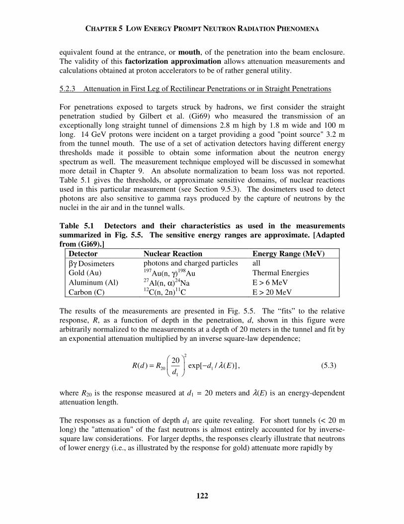
CHAPTER 5 LOW ENERGY PROMPT NEUTRON RADIATION PHENOMENA
122
equivalent found at the entrance, or mouth, of the penetration into the beam enclosure. The validity of this factorization approximation allows attenuation measurements and calculations obtained at proton accelerators to be of rather general utility. 5.2.3 Attenuation in First Leg of Rectilinear Penetrations or in Straight Penetrations For penetrations exposed to targets struck by hadrons, we first consider the straight penetration studied by Gilbert et al. (Gi69) who measured the transmission of an exceptionally long straight tunnel of dimensions 2.8 m high by 1.8 m wide and 100 m long. 14 GeV protons were incident on a target providing a good "point source" 3.2 m from the tunnel mouth. The use of a set of activation detectors having different energy thresholds made it possible to obtain some information about the neutron energy spectrum as well. The measurement technique employed will be discussed in somewhat more detail in Chapter 9. An absolute normalization to beam loss was not reported. Table 5.1 gives the thresholds, or approximate sensitive domains, of nuclear reactions used in this particular measurement (see Section 9.5.3). The dosimeters used to detect photons are also sensitive to gamma rays produced by the capture of neutrons by the nuclei in the air and in the tunnel walls. Table 5.1 Detectors and their characteristics as used in the measurements summarized in Fig. 5.5. The sensitive energy ranges are approximate. [Adapted from (Gi69).]
Detector Nuclear Reaction Energy Range (MeV) βγ Dosimeters photons and charged particles all Gold (Au) 197Au(n, γ)198Au Thermal Energies Aluminum (Al) 27Al(n, α)24Na E > 6 MeV Carbon (C) 12C(n, 2n)11C E > 20 MeV
The results of the measurements are presented in Fig. 5.5. The “fits” to the relative response, R, as a function of depth in the penetration, d, shown in this figure were arbitrarily normalized to the measurements at a depth of 20 meters in the tunnel and fit by an exponential attenuation multiplied by an inverse square-law dependence;
2
20 11
20( ) exp[ / ( )]R d R d E
dλ
= −
, (5.3)
where R20 is the response measured at d1 = 20 meters and λ(E) is an energy-dependent attenuation length. The responses as a function of depth d1 are quite revealing. For short tunnels (< 20 m long) the "attenuation" of the fast neutrons is almost entirely accounted for by inverse-square law considerations. For larger depths, the responses clearly illustrate that neutrons of lower energy (i.e., as illustrated by the response for gold) attenuate more rapidly by
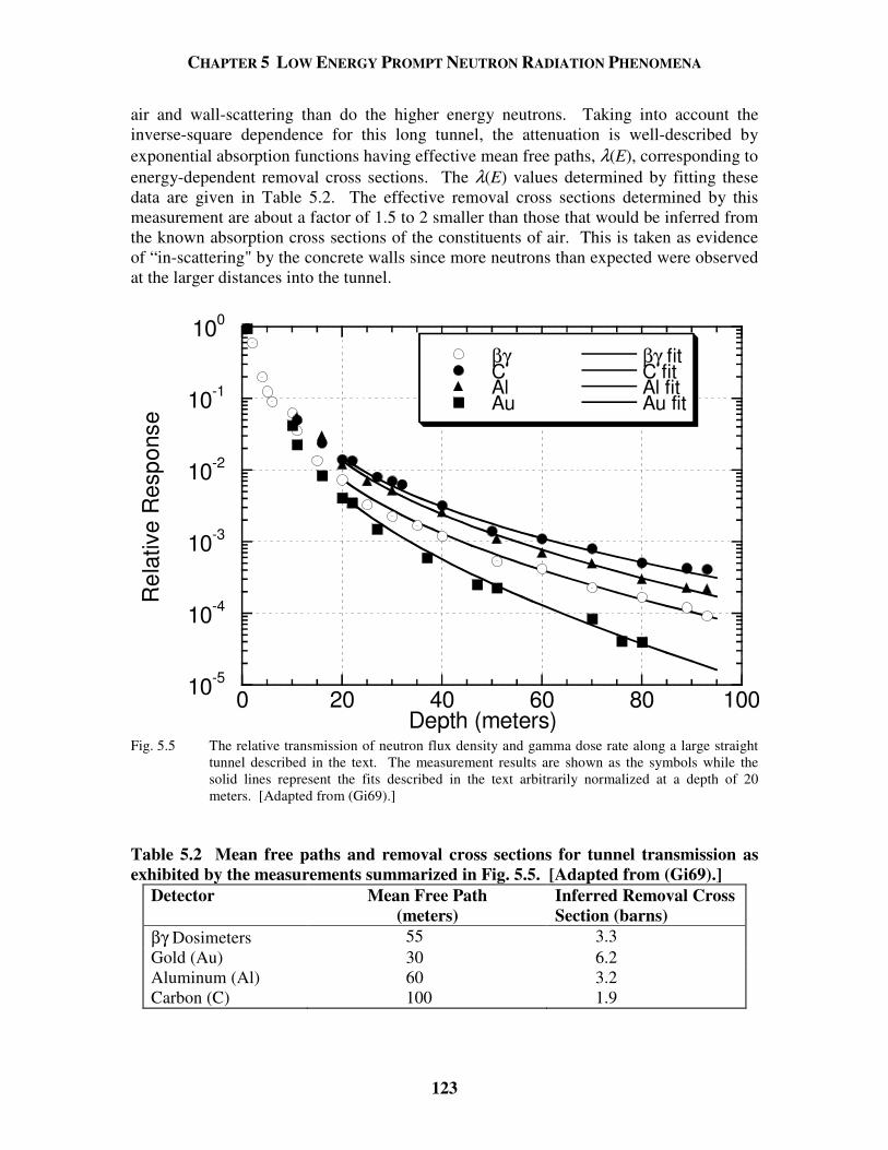
CHAPTER 5 LOW ENERGY PROMPT NEUTRON RADIATION PHENOMENA
123
air and wall-scattering than do the higher energy neutrons. Taking into account the inverse-square dependence for this long tunnel, the attenuation is well-described by exponential absorption functions having effective mean free paths, λ(E), corresponding to energy-dependent removal cross sections. The λ(E) values determined by fitting these data are given in Table 5.2. The effective removal cross sections determined by this measurement are about a factor of 1.5 to 2 smaller than those that would be inferred from the known absorption cross sections of the constituents of air. This is taken as evidence of “in-scattering" by the concrete walls since more neutrons than expected were observed at the larger distances into the tunnel.
10-5
10-4
10-3
10-2
10-1
100
0 20 40 60 80 100
βγCAlAu
βγ fitC fitAl fitAu fit
Rel
ativ
e R
espo
nse
Depth (meters) Fig. 5.5 The relative transmission of neutron flux density and gamma dose rate along a large straight
tunnel described in the text. The measurement results are shown as the symbols while the solid lines represent the fits described in the text arbitrarily normalized at a depth of 20 meters. [Adapted from (Gi69).]
Table 5.2 Mean free paths and removal cross sections for tunnel transmission as exhibited by the measurements summarized in Fig. 5.5. [Adapted from (Gi69).]
Detector Mean Free Path (meters)
Inferred Removal Cross Section (barns)
βγ Dosimeters 55 3.3 Gold (Au) 30 6.2 Aluminum (Al) 60 3.2 Carbon (C) 100 1.9
CHAPTER 5 LOW ENERGY PROMPT NEUTRON RADIATION PHENOMENA
124
An important principle is the labyrinth scaling rule. That is, the attenuation of neutrons in the legs of labyrinths generally scale with a unit length equal to the square root of its cross-sectional area, provided that the height to width ratio does not vary greatly outside of the range 0.5 to 2.0 (Th88). Of course, details of the source geometry are very important in such a straight penetration. Goebel [(Go75) and summarized in (Sc90)] has calculated universal attenuation curves for "first" legs of labyrinths (i.e., those sections first encountered as one moves outward from the beam). Goebel compared results from the codes SAM-CE (Co73), AMC (Ma67), and ZEUS (D'H68). Gollon and Awschalom (Go71) have generated similar curves using the ZEUS code for a variety of geometries. The three situations of point source, line source, and plane or point source off-axis for a straight tunnel displayed as universal dose attenuation curves as calculated by Goebel are given in Fig. 5.6. An off-axis point source is one that is not centered in front of the labyrinth mouth. The distance down the passageway is expressed in units of the square root of the cross-sectional area of the passageway. It is obvious that extended or off-axis sources are more readily attenuated because the tunnel aperture provides a smaller solid angle for acceptance. It has been found by Cossairt (Co95) that Goebel's point source dependence in a tunnel of cross sectional area A can be approximated by the following expression, where δ1 = (d1 - R)/A1/2
and ro is a fitting parameter;
2
1 11
( ) ( )oo
o
rH H R
rδ
δ
= + (5.4)
with ro = 1.4. (5.5)
H1(δ1) is the dose equivalent at distance δ1 in the first leg as measured from the mouth of the passageway in "units" of the square root of the cross-sectional area of the first leg (see Fig. 5.4). Ho(R) is the dose equivalent at the mouth the determination of which will be discussed later. The result of this fit is included in Fig. 5.6. Over the domain of 0 < δ1 < 9 the expression fits the Goebel curve within + 10 per cent, certainly sufficiently accurate for radiation protection purposes. The domain in δ1 is an appropriate one given the fact that most "personnel" labyrinths are of cross-sectional area of about 1 x 2 m2. Hence, a typical unit length is approximately 1.4 meters. A 10 "unit" long first leg is, typically, about 14 meters (or about 46 feet), a distance quite long compared with typical labyrinth legs. Tesch (Te82) has developed a very simple approach to the problem of dose equivalent rate attenuation by multi-legged labyrinths at proton accelerators that are typical of personnel passageways of approximately 2 m2 cross section. For the first leg the expression is an inverse-square law dependence with a simple factor of two included to allow for "in-scattering";
H d H RRd1 1 0
1
2
2( ) ( )=
. (5.6)
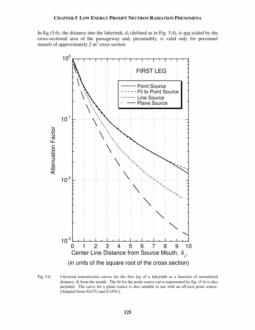
CHAPTER 5 LOW ENERGY PROMPT NEUTRON RADIATION PHENOMENA
125
In Eq (5.6), the distance into the labyrinth, d1 (defined as in Fig. 5.4), is not scaled by the cross-sectional area of the passageway and, presumably, is valid only for personnel tunnels of approximately 2 m2 cross section.
10-3
10-2
10-1
100
0 1 2 3 4 5 6 7 8 9 10
Point SourceFit to Point SourceLine SourcePlane Source
Atte
nuat
ion
Fact
or
Center Line Distance from Source Mouth, δ1,
(in units of the square root of the cross section)
FIRST LEG
Fig. 5.6 Universal transmission curves for the first leg of a labyrinth as a function of normalized
distance, δ1 from the mouth. The fit for the point source curve represented by Eq. (5.4) is also included. The curve for a plane source is also suitable to use with an off-axis point source. [Adapted from (Go75) and (Co95).]
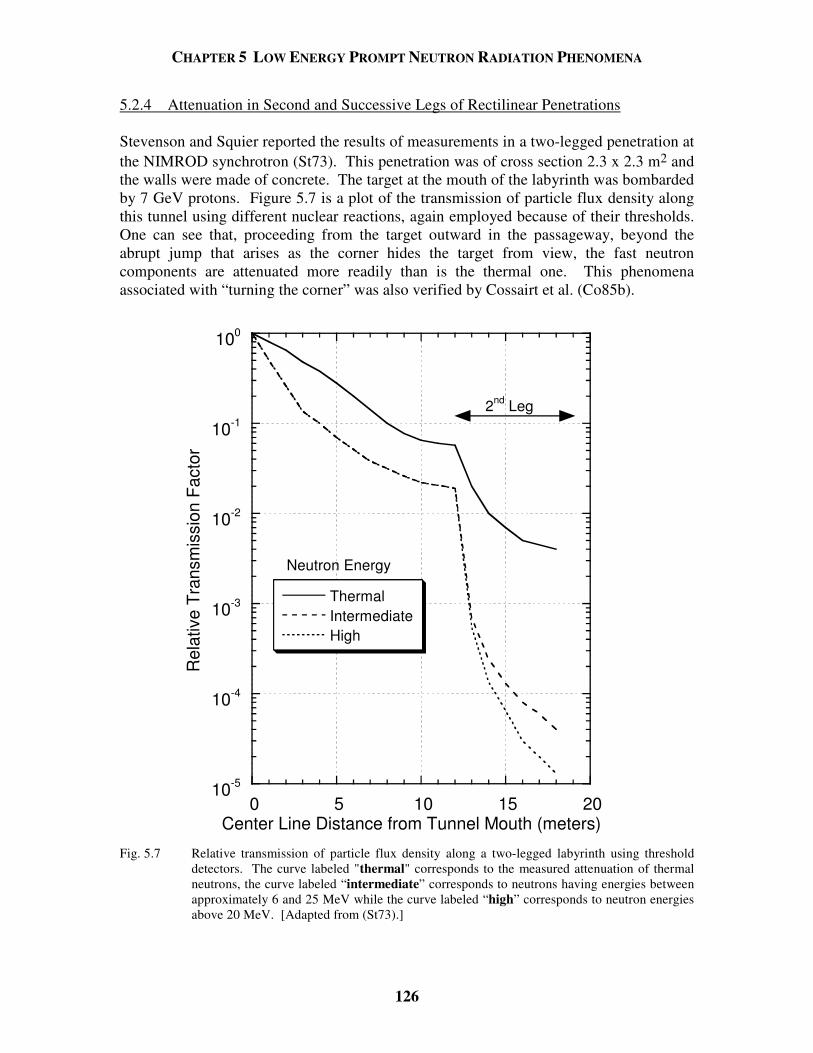
CHAPTER 5 LOW ENERGY PROMPT NEUTRON RADIATION PHENOMENA
126
5.2.4 Attenuation in Second and Successive Legs of Rectilinear Penetrations Stevenson and Squier reported the results of measurements in a two-legged penetration at the NIMROD synchrotron (St73). This penetration was of cross section 2.3 x 2.3 m2 and the walls were made of concrete. The target at the mouth of the labyrinth was bombarded by 7 GeV protons. Figure 5.7 is a plot of the transmission of particle flux density along this tunnel using different nuclear reactions, again employed because of their thresholds. One can see that, proceeding from the target outward in the passageway, beyond the abrupt jump that arises as the corner hides the target from view, the fast neutron components are attenuated more readily than is the thermal one. This phenomena associated with “turning the corner” was also verified by Cossairt et al. (Co85b).
10-5
10-4
10-3
10-2
10-1
100
0 5 10 15 20
ThermalIntermediateHigh
Rel
ativ
e Tr
ansm
issi
on F
acto
r
Center Line Distance from Tunnel Mouth (meters)
Neutron Energy
2nd Leg
Fig. 5.7 Relative transmission of particle flux density along a two-legged labyrinth using threshold
detectors. The curve labeled "thermal" corresponds to the measured attenuation of thermal neutrons, the curve labeled “intermediate” corresponds to neutrons having energies between approximately 6 and 25 MeV while the curve labeled “high” corresponds to neutron energies above 20 MeV. [Adapted from (St73).]
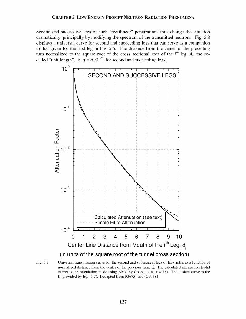
CHAPTER 5 LOW ENERGY PROMPT NEUTRON RADIATION PHENOMENA
127
Second and successive legs of such "rectilinear" penetrations thus change the situation dramatically, principally by modifying the spectrum of the transmitted neutrons. Fig. 5.8 displays a universal curve for second and succeeding legs that can serve as a companion to that given for the first leg in Fig. 5.6. The distance from the center of the preceding turn normalized to the square root of the cross sectional area of the ith leg, Ai, the so-called “unit length”, is δi = di /A1/2, for second and succeeding legs.
10-4
10-3
10-2
10-1
100
Calculated Attenuation (see text)Simple Fit to Attenuation
0 1 2 3 4 5 6 7 8 9 10
Atte
nuat
ion
Fact
or
SECOND AND SUCCESSIVE LEGS
Center Line Distance from Mouth of the i th Leg, δi
(in units of the square root of the tunnel cross section)
Fig. 5.8 Universal transmission curve for the second and subsequent legs of labyrinths as a function of normalized distance from the center of the previous turn, δi. The calculated attenuation (solid curve) is the calculation made using AMC by Goebel et al. (Go75). The dashed curve is the fit provided by Eq. (5.7). [Adapted from (Go75) and (Co95).]
CHAPTER 5 LOW ENERGY PROMPT NEUTRON RADIATION PHENOMENA
128
It was found by Cossairt (Co95) that the following recursive expression adequately describes this curve, where δi is the distance in the ith leg measured in "units" of the square root of the cross-sectional area of the ith leg:
1 1
exp( / ) exp( / ) exp( / )( ) ( )
1i i i
i i i i
a A b B cH H
A Bδ δ δδ δ− −
− + − + − = + + ith leg (i > 1),
(5.7) where the fitting parameters are; a = 0.17, A = 0.21,
b = 1.17, and B = 0.00147. c = 5.25, The results of this fit are included in Fig. 5.8. Tesch (Te82) also has developed a formula for the transmission of the second and successive legs which is
H dd A d
AHi i
i i i
ii( )
exp( / . ) . exp( / . )
.
.
.=− + −
+
−
0 45 0 022 2 35
1 0 022
13
13 1 (ith leg, i > 1) (5.8)
Here Ai is the cross sectional area of the ith leg in units of square meters. As was the case with respect to Eq. (5.6), this formula uses the distances, di (meters), along the labyrinth directly and does not scale them against the square root of the cross sectional area. As was the case for Eq. (5.6), the results are valid for “door-sized” labyrinths having cross sectional areas of approximately 2 m2. Figure 5.9 shows a four-legged labyrinth providing entrance to a tunnel above a target struck by 400 GeV protons accelerated by the Tevatron at Fermilab. Figure 5.10 compares experimental measurements (Co85b) of absorbed dose throughout this labyrinth with several methods of calculation. As one can see, all methods of calculating the attenuation discussed here are approximately valid even for this four-legged labyrinth. Even the first leg, while not quite having a truly “open view” of the target is handled well by these methods. Thus, the assumption that succeeding legs can be considered the same as the second leg is verified.12 For this labyrinth, a recombination chamber technique (see Section 9.5.7) was used to measure the neutron quality factor, Q, at two locations, one at the end of the first leg and one in the middle of the short second leg. These locations are denoted by R in Fig. 5.9. The results were Q = 5.5 + 0.6 (first leg) and Q = 3.4 + 0.1 (second leg). This indicates a reduction of the average neutron energy in the second leg which was further verified by a
12In the labyrinth shown in Fig. 5.9, the shielding blocks were, in fact, aligned as indicated. This is contrary to good design practice as the blocks should have been overlapped to prevent “streaming”. This condition may well explain the excess of measurement over calculation at the end of the third leg.
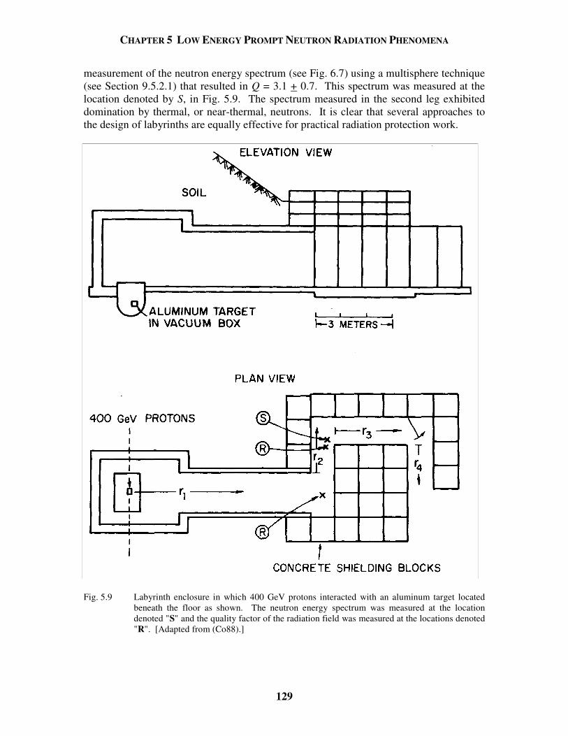
CHAPTER 5 LOW ENERGY PROMPT NEUTRON RADIATION PHENOMENA
129
measurement of the neutron energy spectrum (see Fig. 6.7) using a multisphere technique (see Section 9.5.2.1) that resulted in Q = 3.1 + 0.7. This spectrum was measured at the location denoted by S, in Fig. 5.9. The spectrum measured in the second leg exhibited domination by thermal, or near-thermal, neutrons. It is clear that several approaches to the design of labyrinths are equally effective for practical radiation protection work.
Fig. 5.9 Labyrinth enclosure in which 400 GeV protons interacted with an aluminum target located beneath the floor as shown. The neutron energy spectrum was measured at the location denoted "S" and the quality factor of the radiation field was measured at the locations denoted "R". [Adapted from (Co88).]
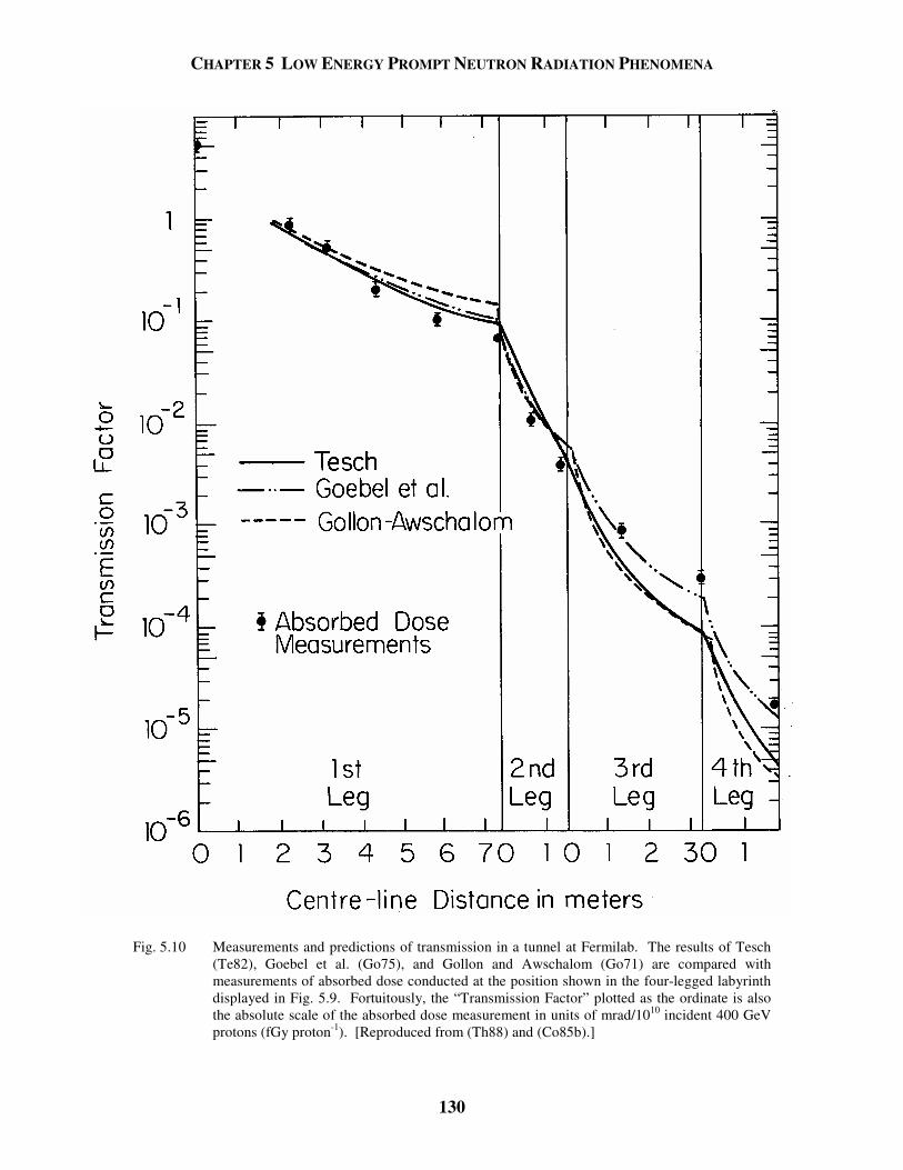
CHAPTER 5 LOW ENERGY PROMPT NEUTRON RADIATION PHENOMENA
130
Fig. 5.10 Measurements and predictions of transmission in a tunnel at Fermilab. The results of Tesch
(Te82), Goebel et al. (Go75), and Gollon and Awschalom (Go71) are compared with measurements of absorbed dose conducted at the position shown in the four-legged labyrinth displayed in Fig. 5.9. Fortuitously, the “Transmission Factor” plotted as the ordinate is also the absolute scale of the absorbed dose measurement in units of mrad/1010 incident 400 GeV protons (fGy proton-1). [Reproduced from (Th88) and (Co85b).]
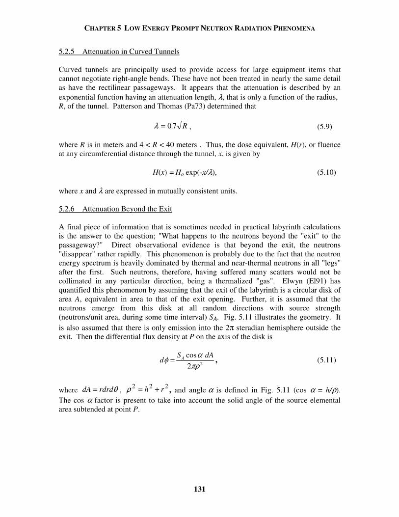
CHAPTER 5 LOW ENERGY PROMPT NEUTRON RADIATION PHENOMENA
131
5.2.5 Attenuation in Curved Tunnels Curved tunnels are principally used to provide access for large equipment items that cannot negotiate right-angle bends. These have not been treated in nearly the same detail as have the rectilinear passageways. It appears that the attenuation is described by an exponential function having an attenuation length, λ, that is only a function of the radius, R, of the tunnel. Patterson and Thomas (Pa73) determined that λ = 0 7. R , (5.9) where R is in meters and 4 < R < 40 meters . Thus, the dose equivalent, H(r), or fluence at any circumferential distance through the tunnel, x, is given by H(x) = Ho exp(-x/λ), (5.10) where x and λ are expressed in mutually consistent units. 5.2.6 Attenuation Beyond the Exit A final piece of information that is sometimes needed in practical labyrinth calculations is the answer to the question; "What happens to the neutrons beyond the "exit" to the passageway?" Direct observational evidence is that beyond the exit, the neutrons "disappear" rather rapidly. This phenomenon is probably due to the fact that the neutron energy spectrum is heavily dominated by thermal and near-thermal neutrons in all "legs" after the first. Such neutrons, therefore, having suffered many scatters would not be collimated in any particular direction, being a thermalized "gas". Elwyn (El91) has quantified this phenomenon by assuming that the exit of the labyrinth is a circular disk of area A, equivalent in area to that of the exit opening. Further, it is assumed that the neutrons emerge from this disk at all random directions with source strength (neutrons/unit area, during some time interval) SA. Fig. 5.11 illustrates the geometry. It is also assumed that there is only emission into the 2π steradian hemisphere outside the exit. Then the differential flux density at P on the axis of the disk is
2
cos 2
AS dAd
αφπρ
= , (5.11)
where θrdrddA = , 222 rh +=ρ , and angle α is defined in Fig. 5.11 (cos α = h/ρ). The cos α factor is present to take into account the solid angle of the source elemental area subtended at point P.
CHAPTER 5 LOW ENERGY PROMPT NEUTRON RADIATION PHENOMENA
132
Fig. 5.11 Diagram of labyrinth exit neutron calculation. The coordinates are explained in the text. Thus,
32
AS hrd drdφ θ
πρ= . (5.12)
Integrating,
( ) ( )2
3/ 2 3/ 20 0 02 2 2 2( )
2
R RA
A
S h r rh dr d S h dr
r h r h
πφ θ
π= = =
+ +
2 2 20
1 11 ,
1
R
A AS h Sr h R
h
− = − + + (5.13)
where attenuation by the air is neglected. Thus one can use this by approximating the area of the exit opening by the area of a disk have an equivalent area. At large distances, one can apply a "point source" approximation due to the fact that
φ( )hS R
hA≈
2
2
for h >> R. (5.14)
For h = 0, φ (0) = SA as expected. This calculation neglects neutron absorption by the intervening air. The rapidity of the decrease of fluence is illustrated by the tabulation of a few values in Table 5.3.
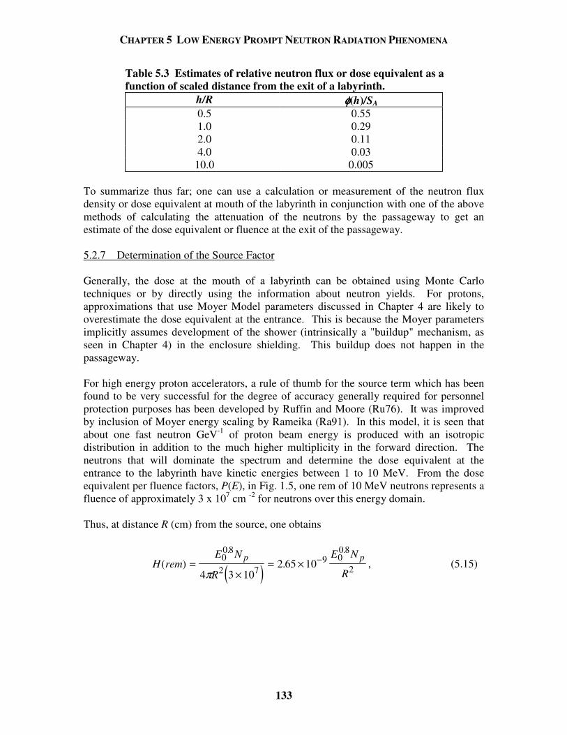
CHAPTER 5 LOW ENERGY PROMPT NEUTRON RADIATION PHENOMENA
133
Table 5.3 Estimates of relative neutron flux or dose equivalent as a function of scaled distance from the exit of a labyrinth.
h/R φφφφ(h)/SA 0.5 0.55 1.0 0.29 2.0 0.11 4.0 0.03
10.0 0.005 To summarize thus far; one can use a calculation or measurement of the neutron flux density or dose equivalent at mouth of the labyrinth in conjunction with one of the above methods of calculating the attenuation of the neutrons by the passageway to get an estimate of the dose equivalent or fluence at the exit of the passageway. 5.2.7 Determination of the Source Factor Generally, the dose at the mouth of a labyrinth can be obtained using Monte Carlo techniques or by directly using the information about neutron yields. For protons, approximations that use Moyer Model parameters discussed in Chapter 4 are likely to overestimate the dose equivalent at the entrance. This is because the Moyer parameters implicitly assumes development of the shower (intrinsically a "buildup" mechanism, as seen in Chapter 4) in the enclosure shielding. This buildup does not happen in the passageway. For high energy proton accelerators, a rule of thumb for the source term which has been found to be very successful for the degree of accuracy generally required for personnel protection purposes has been developed by Ruffin and Moore (Ru76). It was improved by inclusion of Moyer energy scaling by Rameika (Ra91). In this model, it is seen that about one fast neutron GeV-1 of proton beam energy is produced with an isotropic distribution in addition to the much higher multiplicity in the forward direction. The neutrons that will dominate the spectrum and determine the dose equivalent at the entrance to the labyrinth have kinetic energies between 1 to 10 MeV. From the dose equivalent per fluence factors, P(E), in Fig. 1.5, one rem of 10 MeV neutrons represents a fluence of approximately 3 x 107 cm -2 for neutrons over this energy domain. Thus, at distance R (cm) from the source, one obtains
( )H remE N
R
E N
R
p p( ) .
. .
=×
= × −00 8
2 79 0
0 8
24 3 102 65 10
π, (5.15)
CHAPTER 5 LOW ENERGY PROMPT NEUTRON RADIATION PHENOMENA
134
where Eo is in GeV, and Np is the number of incident protons. The constant, 2.65 x 10⁻⁹
(rem cm2), turns out to be approximately one-third the value obtained by using the Moyer source parameter along with high energy value of the Moyer angular factor at θ = π /2 [Eqs. (4.38) and (4.41)];
(2.8 x 10⁻⁷ rem cm2)exp(-2.3π /2) = 7.6 x 10⁻⁹ rem cm2. (5.16) To obtain the source factor for neutrons produced by electrons, the neutron yields discussed in Section 3.2.4 can be utilized. 5.3 Skyshine Thin roof shielding represents a serious problem that has plagued a number of accelerators such as the Cosmotron (at Brookhaven National Laboratory), the Bevatron (at the Lawrence Berkeley National Laboratory), the Fermilab experimental areas, and likely elsewhere. The phenomenon, known as skyshine, is the situation in which the roof of some portion of the accelerator or an associated experimental facility is shielded more thinly than are the sides of the same enclosure that directly view the radiation source. The first attempt to calculate the skyshine radiation field was made by Lindenbaum (Li61). Schopper et al. (Sc90) give a rather complete description of the phenomena and Patterson and Thomas (Pa73), Rindi and Thomas (Ri75), Stevenson and Thomas (St84a), and Cossairt and Coulson (Co85c) present some specific results. Neutron skyshine, while it is usually "preventable" through the application of sufficient roof shielding, has been encountered at nearly all major accelerators. This has resulted either from lack of consideration of it at the design stage or from the need to accommodate other constraints such as the need to minimize the weight of shielding borne by the roofs of large experimental halls. Also, due to the creative efforts of many physicists and engineers the beam intensities eventually available at accelerators have often greatly exceeded those credible at the time at the initial design. 5.3.1 Simple Parameterizations When addressing the skyshine question, it is generally customary to plot the neutron fluence, or even the dose equivalent, as a function of distance from the source by multiplying it by the square of the distance from the source, i.e. as r2Φ (r). Stevenson and Thomas (St84a) included plots of a number of measurements of neutron skyshine obtained at proton accelerators producing protons of energies ranging from 30 MeV to 30 GeV, and also at high energy electron accelerators having energies of 7.5 and 12 GeV. In general, the quantity r2Φ (r) is characterized by a buildup followed by an exponential falloff. Most skyshine distributions are isotropic at ground level (i.e., independent direction with respect to the beam axis). As exhibited by the typical skyshine data, λ, the effective attenuation length, has been found to vary between a minimum value of about 200 meters and much larger values which approach one kilometer. We shall shortly see how this quantity is dependent upon the energy spectrum of the neutron radiation field that is the source of the skyshine.
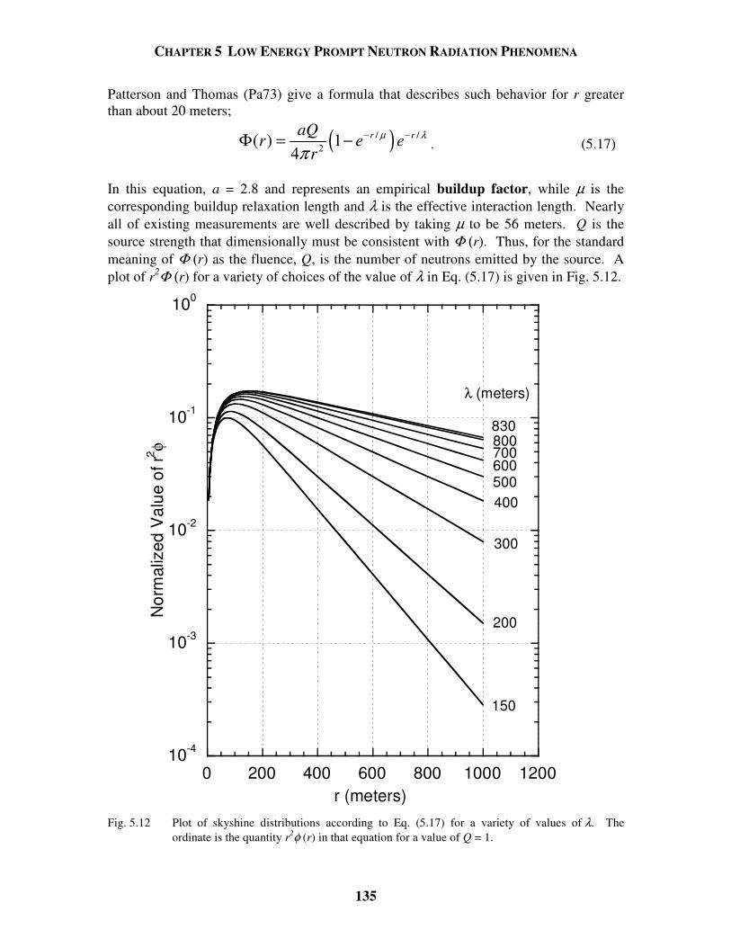
CHAPTER 5 LOW ENERGY PROMPT NEUTRON RADIATION PHENOMENA
135
Patterson and Thomas (Pa73) give a formula that describes such behavior for r greater than about 20 meters;
( )/ /2( ) 1
4r raQ
r e er
µ λ
π− −Φ = − . (5.17)
In this equation, a = 2.8 and represents an empirical buildup factor, while µ is the corresponding buildup relaxation length and λ is the effective interaction length. Nearly all of existing measurements are well described by taking µ to be 56 meters. Q is the source strength that dimensionally must be consistent with Φ (r). Thus, for the standard meaning of Φ (r) as the fluence, Q, is the number of neutrons emitted by the source. A plot of r2Φ (r) for a variety of choices of the value of λ in Eq. (5.17) is given in Fig. 5.12.
10-4
10-3
10-2
10-1
100
0 200 400 600 800 1000 1200
Nor
mal
ized
Val
ue o
f r2 φ
r (meters)
λ (meters)
830800700600500400
300
200
150
Fig. 5.12 Plot of skyshine distributions according to Eq. (5.17) for a variety of values of λ. The
ordinate is the quantity r2φ (r) in that equation for a value of Q = 1.
CHAPTER 5 LOW ENERGY PROMPT NEUTRON RADIATION PHENOMENA
136
Values of λ > 830 meters are possible if very high energy neutrons (E >> 150 MeV) are present. A value of 830 m (100 g cm-2 of air at standard temperature and pressure) corresponds to the interaction length of the neutrons of approximately 100 MeV likely to control the propagation of hadronic cascades in air. Thus, λ is determined by the neutron energy spectrum present at the thinly shielded location. Larger values of λ are more plausibly due to multiple sources or an extended source. In such circumstances, the radiation field may also not necessarily be isotropic. Cossairt and Coulson (Co85c) present an example of a non-isotropic, complex skyshine source involving high energies, an extended source, and an extremely thin shield that resulted in a value of λ ≈ 1200 meters. The procedure, then, for using Eq. (5.17) is to do the following: A. Estimate the total emission rate of neutrons from the source. This can be done by
using information about the neutron spectrum at the source to choose an "average" energy and intensity. The dose equivalent per fluence conversion factor at that energy can then be used in conjunction with a dose equivalent rate survey over the thinly shielded region to determine the total neutron emission rate, Q, by numerically integrating over the area of the top of the shield.
B. Estimate the value of λ from the neutron energy spectrum information. C. Apply Eq. (5.17) to determine the radial dependence. 5.3.2 A Somewhat More Rigorous Treatment A somewhat more rigorous treatment has been reported by Stevenson and Thomas (St84a) that is based on the work of Alsmiller, Barish, and Childs (Al81) and Nakamura and Kosako (Na81). These groups have independently performed extensive calculations of the neutrons emitted into cones of small vertex angle. Alsmiller, Barish, and Childs used the Discrete Ordinates Transport (DOT) Code while Nakamura and Kosako used the Monte Carlo code MORSE. For selected distances from the skyshine source, these workers have calculated the dose equivalent as a function of both the source neutron energy and the emission cone's semivertical angle (that is, the half-angle the rotation of which defines the cone into which the neutrons are emitted). The authors define this quantity, the so-called neutron importance, as the dose equivalent per emitted neutron as a function of the energy of the emitted neutron and of the distance from the source. This quantity is a measure of how “important” a given emitted neutron is in delivering radiation dose equivalent to a point in space located at a given distance from the skyshine source. The results of the Alsmiller calculation for small semivertical angles are given in Fig. 5.13. Numerical tabulations of neutron importance functions according to (Al81) are provided in references (NC03) and (Th88). The corresponding, but somewhat less-detailed results of Nakamura, are in good agreement with these results.
CHAPTER 5 LOW ENERGY PROMPT NEUTRON RADIATION PHENOMENA
137
10-23
10-22
10-21
10-20
10-19
10-18
10-17
10-7 10-6 10-5 10-4 10-3 10-2 10-1 100 101 102 103
Neu
tron
Impo
rtan
ce (r
em n
eutro
n-1)
Neutron Energy (MeV)
r = 108 meters
r = 495 meters
r = 1005 meters
Fig. 5.13 Top frame: The definition of the semivertical cone angle used in skyshine calculations of
Alsmiller et al. (Al81). Bottom frame: Neutron skyshine importance functions for a semivertical cone angle of 37o at three different values of the distance from a point source. [Adapted from Alsmiller et al. (Al81)].

CHAPTER 5 LOW ENERGY PROMPT NEUTRON RADIATION PHENOMENA
138
Stevenson and Thomas (St84a) were able to derive an alternative "recipe" for skyshine neutron calculations to that expressed in Eq. (5.17) by making two assumptions: A. The neutron energy spectrum has the 1/E form up to the proton energy and zero at
higher energies. This likely overestimates the contribution of the higher energy neutrons.
B. The neutrons are emitted into a cone whose semivertical angle is about 35 to 40o.
This may overestimate the doses by up to a factor of three for sources of smaller semivertical angles.
Stevenson and Thomas parameterized the skyshine phenomena using the following equation:
/2( )
4 rQ
r er
λ
π−′
Φ = . (5.18)
In this equation, the buildup exponential factor has been suppressed so the formula is valid only at large distances (i.e., r >> 56 meters). In addition, the source strength denoted by Q′ implicitly includes the buildup factor of 2.8. Further, they used the Alsmiller importance functions to estimate the value of λ based upon the upper energy (i.e., cutoff energy) of the 1/E spectrum. Fig. 5.14 displays the results of doing this for several choices of upper energies at three distances in a plot in which the inverse-square dependence is suppressed. A comparison with a measurement conducted at Brookhaven National Laboratory is also provided.
10-16
10-15
10-14
10-13
0 200 400 600 800 1000 1200
r2 H (
rem
m2 n
eutro
n-1)
r (meters)
BNL400 MeV125 MeV
45 MeV
12.2 MeV
4.5 MeV
1.1 MeV
Fig. 5.14 Variation of dose equivalent with distance r for 1/E neutron spectra with different upper
energies. The ordinate is dose equivalent H times r2. The curve labeled "BNL" is the result of a measurement at the Brookhaven National Laboratory Alternating Gradient Synchrotron, a 30 GeV proton accelerator. [Adapted from (St84a).]
CHAPTER 5 LOW ENERGY PROMPT NEUTRON RADIATION PHENOMENA
139
The slopes, then, were used to obtain theoretical values of λ as a function of "upper energy" which are plotted in Fig. 5.15.
0
200
400
600
800
1000
100 101 102 103 104 105
λ (m
eter
s)
Upper Energy of 1/E Spectrum (MeV)
Fig. 5.15 Effective absorption length λ as a function of upper neutron energy E for 1/E spectra. [Adapted from (St84a).]
To determine the source term, the straight lines in Fig. 5.14 (on the semi-logarithmic plot) were extrapolated to zero and used to determine intercepts at r = 0 ranging from 1.5 x 10⁻¹⁵ to 3 x 10-15 Sv m2/neutron (1.5 x 10⁻¹³ to 3 x 10-13 rem m2/neutron). Hence, conservatively, Stevenson and Thomas found that, over a rather large range of incident proton energies spatial dependence of the dose equivalent, H(r) can be described by
λ/
2
13e
103)( r
rrH −
−×= (rem/emitted neutron, r in meters). (5.19)
Again, one has to determine the total number of neutrons emitted. This can be done as before by measuring the integral of dose equivalent times the area over the thinly shielded location and using the reciprocal of the dose equivalent per fluence conversion factor appropriate for the neutron energy spectrum at hand to get the total number of neutrons emitted. The use of Eq. (5.19) will lead to an overestimate of neutrons for values of r less than approximately 100 meters because the extrapolation ignores the observed exponential buildup of the skyshine. Stevenson and Thomas (St84a) give a convenient table, useful for general purposes, of dose equivalent per fluence conversion factors derived from data in ICRP Publication 21 (IC73) integrated over such 1/E spectra which is provided here as Table 5.4.
CHAPTER 5 LOW ENERGY PROMPT NEUTRON RADIATION PHENOMENA
140
Table 5.4 Dose equivalent per neutron/cm2 for 1/E neutron spectra of different upper energies. [Adapted from (St84a).] Upper Energy Spectrum Averaged Dose Equivalent Conversion (MeV) (10-9rem cm2/neutron) 1.6 3.9 2.5 4.8 4.0 5.6 6.3 6.4 10 7.2 16 7.9 25 8.6 40 9.4 63 10.1 100 10.9 160 11.7 250 12.5 400 13.4 630 14.6 1000 16.2 1600 18.4 2500 21.2 4000 25.0 6300 30.0 10000 36.5
5.3.3 Examples of Experimental Verifications Measurements at Fermilab (Co85c) have confirmed the validity of these methods for a "source" involving the targetry of 400 GeV protons. Figure 5.16 shows two measured and fitted radial distributions made using Eq. (5.17). In Fig. 5.16 "Survey 2" corresponds to a shielding configuration where the neutron energy spectrum was inferred to be of very high energy while "Survey 4" was likely to involve a much less energetic spectrum. Survey 4 was made for the same beam and target after the concrete shield thickness around the source was greatly increased compared with the shield present when "Survey 2" was obtained. The normalization to "COUNTS-M2 HR-1" refers to an integration of an instrumental response over the surface area of the source and should be approximately proportional to the emitted neutron fluence. The instrument calibration of "COUNTS/HR" made possible an estimate of the dose equivalent at r = 200 meters for the two surveys. In view of details of the conditions not described in detail here, one can make an educated guess that the spectrum of emitted neutrons of "Survey 2" had an upper energy of ≈ 1 GeV, while the spectrum of emitted neutrons of "Survey 4" had an upper energy of ≈ 100 MeV.
CHAPTER 5 LOW ENERGY PROMPT NEUTRON RADIATION PHENOMENA
141
Fig. 5.16 Skyshine data from two different surveys plotted as r2φ as a function of distance from the
source r. The solid curves are from the least squares fit of Eq. (5.17) to the data points while the dashed curve is the fit if λ is constrained to have a value of 830 m. Error bars represent one standard deviation counting statistics. [Reproduced from (Co85c).]
Using the appropriate dose equivalent per fluence conversion factor, the value of Q for the Survey 2 conditions was determined experimentally to be 2.5 x 10⁵ mrem m2 hr-1. This was obtained from the measured absorbed dose surface integral of 5 x 10⁴ mrad m2hr-1 and assumed a quality factor of 5. For the Survey 4 conditions, Q was found to be 4.0 x 10⁴ mrem m2 hr-1. Again, this was obtained from the measured absorbed dose surface integral of 8.1 x 10³ mrad m2 hr-1 and assumed a quality factor of 5. Table 5.5 makes a comparison with the prescription of (St84a) for these data. In this table H is the dose equivalent in one hour at 200 meters. The prescription of Stevenson and Thomas (St84a) is used to calculate the dose equivalent in one hour at 200 meters. The agreement is well within all uncertainties involved.
CHAPTER 5 LOW ENERGY PROMPT NEUTRON RADIATION PHENOMENA
142
Table 5.5 Comparisons of Fermilab skyshine data with results of parameterizations of surveys shown in Fig. 5.16, assuming 1/E spectra with inferred upper energies. The quantities are all for a one hour time period.
Survey λλλλ (meters) (Co85c)
Emax (inferred)
(MeV)
Dose Equiv. per
Fluence (mrem/ n cm-2) (St84a)
Qmeasured (mrem m2)
(Co85c)
H (200 m) (mrem)-
calculated
H (200 m) (mrem)-
measured (Co85c)
Survey 2 1200 1000 16.2 x 10⁻⁶ 2.5 x 10⁵ 1.0 1.6 Survey 4 340 100 10.9 x 10⁻⁶ 4.0 x 10⁴ 0.15 0.15 Another illustration is provided by Elwyn and Cossairt (El86) in connection with neutron radiation field emerging from an iron shield that is more fully described in Section 6.3.5. Fig. 5.17 taken from (El86) shows the measured radial dependence of neutron flux as a function of distance from that iron shield.
Fig. 5.17 The product of r2 and the neutron fluence φ (r) per 1012 protons incident on a target as a
function of the distance from the source r. The source is that described in connection with Fig. 6.8. The smooth curve is a fit to Eq. (5.17) with parameters λ = 184.4 m and Q = 1.74 x 10¹⁰ neutrons per 1012 protons. [Reproduced from (El86).]
CHAPTER 5 LOW ENERGY PROMPT NEUTRON RADIATION PHENOMENA
143
From other considerations pertaining to an iron shield discussed in Section 6.3.5, it is known that the radiation field is dominated by neutrons of energies near 847 keV. Using the measured data, normalized to 1012 incident protons the parameters Q = 1.75 x 10¹⁰ and λ = 184.4 meters were determined by fitting the skyshine data using Eq. (5.17). Evaluating Φ at r = 200 meters,
[ ] 2-42
10m neutrons 1020.3)4.184/200exp()56/200exp(1
)200( 4
)1075.1(8.2)200( ×=−−×=Φ
π.
(5.20)
Thus, taking the measured neutron flux at r = 200 meters and applying a dose equivalent per fluence value of 3.0 x 10⁻⁵ mrem cm-2 appropriate for 847 keV neutrons (see Fig. 1.5) gives a dose equivalent per 1012 incident protons of 9.6 x 10⁻⁵ mrem at r = 200 meters. The value of λ that fitted the skyshine data is also consistent with the neutron energy spectrum, which was known to be dominated by neutrons of about 1 MeV kinetic energy.
Elwyn and Cossairt also estimated a value of (3.4 + 2.0) x 1010 per 1012 incident protons for the total neutron emission of the source by performing a numerical integration over the surface area of the source, separate from the result determined using the skyshine measurement. Applying the prescription of Stevenson and Thomas (St84a) found in Eq. (5.18);
H( )( )[( . . ) ]
( )exp( / . )200
3 10 34 2 0 10
200200 184 4
13 10
2=× ± ×
− =−
= (8.6 + 5.1) x 10-5 mrem per 1012 protons (5.21) at this same location. This result is very consistent with that found using Eq. (5.20).
CHAPTER 5 LOW ENERGY PROMPT NEUTRON RADIATION PHENOMENA
144
Problems 1. A 1 µA 100 MeV electron beam is incident on an "optimized bremsstrahlung"
target in a shielding configuration and labyrinth like that in Fig. 5.3. Using the facts given in Chapter 3 (Swanson's Rules of Thumb, etc.) about bremsstrahlung, calculate the dose equivalent rate at the exit of a labyrinth having 2 legs. Set all distances di, d1, and d2 = 3 meters. If the goal is to get the dose equivalent rate at the exit to be < 1 mrem/hr, is this a sensible design? The 2 legs are 1 x 2 meter2 in cross section and, since no other information is available, use α = 10-2 as a "conservative" value. For purposes of this problem, photons constitute the only component of radiation present. [Hint: One needs to calculate the projected diameter of the beam at the wall where the first scatter occurs. This can be done using Eq. (3.12).]
2. A 500 GeV proton beam of 1011 protons/second strikes a magnet 2 m from the
mouth of a 3-legged labyrinth. Each of the 3 legs is 4 meters long and 1 x 2 m2 in cross section. The length of leg 1 is measured from the mouth of the labyrinth to the center of the first turn, all other lengths are measured between centers of turns. Assume the source is an on-axis “point source”. Using Goebel's "universal" curves and Rameika's source term, what is the dose equivalent rate at the exit expressed in rem hr-1. How far away from the exit does the value of dH/dt fall to 10 mrem hr-1.
3. A high energy accelerator has a section of beamline which was poorly designed.
Beam losses and insufficient shielding have resulted in a region of roof 10 meters wide and 50 meters long where a neutron dose equivalent rate averaging 100 mrem/hour (averaged over the surface of the weak shield) is found. A spectrum measurement indicates the spectrum to be approximately 1/E with an upper end point of approximately 500 MeV. Calculate the dose equivalent rate due to skyshine at distance r = 50, 100, 200, 500, & 1000 m using both formulae presented here.
CHAPTER 6 SHIELDING MATERIALS AND NEUTRON ENERGY SPECTRA
145
6.1 Introduction After all of this discussion of the production of prompt radiation at accelerators, it is now advisable to review in one place the relevant properties of the most common materials used in radiation shielding. Since many shielding problems are driven by the nature of the energy spectrum of the neutrons, such spectra are also discussed here in some detail and examples of neutron energy spectra measured external to shielding at various types of accelerator facilities are presented. 6.2 Discussion of Shielding Materials Commonly Used at Accelerators Given the size of many modern accelerators, economic considerations commonly dominate shielding designs; requiring the use of relatively relatively inexpensive, but often less than optimally efficient shields. Aside from the need to accomplish the identified goals in radiation safety, in all situations good engineering practices concerning structural properties, appropriate floor loading allowances, and fire protection must be taken into account to provide an acceptable level of occupational and public safety. In general, low atomic number materials are best used for targets, collimators, and beam stops at electron accelerators to reduce photon production, while high atomic number materials are preferred at proton and heavy ion accelerators for these components to reduce neutron production. From the previous chapters, it should be clear that at beam energies above 5 MeV neutrons are produced in most materials. Some materials have superior heat transfer characteristics that enhance durability and reliability and thus can reduce personnel exposures incurred in maintenance activities. 6.2.1 Earth Earth has many admirable qualities as a shield material besides its low cost. Especially important is the fact that the water it contains enhances the effectiveness of the neutron attenuation. This is because the mass of a proton is essentially equal to that of a neutron, a fact that facilitates the transfer of energy from the particle to the shielding medium. As a result of conservation of energy and momentum, in an elastic collision the energy ∆E that can be transferred from a neutron having kinetic energy Eo to a target nucleus as a function of scattering angle θ is given by
2
2
4 cos
1
n
o
n
MmE
E Mm
θ∆ =
+
, (6.1)
where M is the mass of the recoiling nucleus and mn is the mass of the incident neutron. Thus, at small scattering angles (i.e., θ ≈ 0), nearly all of the neutron kinetic energy can be transferred to the protons in the water. For comparison, 12C nuclei are capable of absorbing only 28 per cent of the incident neutron energy. The proton energy, then, can
CHAPTER 6 SHIELDING MATERIALS AND NEUTRON ENERGY SPECTRA
146
be dissipated in the medium by means of ionization and nuclear interactions. Representative ranges of soil water content (per cent of dry weight) for different soil types are; sand (0-10), sandy loam (5-20), loam (8-25), silty loam (10-30), dry loam (14-30), and clay (15-30). Additionally, earth is also composed of sufficiently high atomic number elements to be effective against photons. Dry earth has a typical elemental composition as given in Table 6.1. Earth is generally a "crackless" shield, not prone to neutron leakage by "streaming". The density of earth varies widely, from as low as 1.7 g cm-3 to as much as 2.25 g cm-3, depending upon soil type and water content. In general, sandy soils will have lower values of density than heavy clays found in glacial till. Extrusive volcanic soils, on the other hand, can have very low densities. Given this variation, specific knowledge of soil characteristics at the accelerator site are needed to do effective shielding designs. Definitive measurements of the soil water content are also most useful if the shielding of neutrons is the intent and no safety factors are being used.
Table 6.1 Elemental composition, dry-weight per cent, of representative soils. [Adapted from (Ch84).]
Element Global Average (%) O 43.77 Si 28.1 Al 8.24 Fe 5.09 Mn 0.07 + 0.06 Ti 0.45 + 0.43 Ca 3.65 Mg 2.11 K 2.64 Na 2.84
6.2.2 Concrete Concrete has obvious advantages in that it can either be poured in place permanently or be cast into modular blocks. It has considerable structural strength and steel reinforcement has essentially no effect on the shielding properties. Sometimes concrete blocks are used to shield targets, beam stops, etc. in a manner that allows their ready access if the need for maintenance arises. The use of concrete blocks generally requires their overlapping to avoid streaming through the cracks. It is sometimes efficient to use a heavy material as part of the aggregate in the concrete recipe. This can increase the concrete density as well as its average atomic number. The latter, of course, increases the effectiveness against photons. Table 6.2 due to Chilton (Ch84) gives some partial densities of various concretes used in shielding, thus illustrating the elemental variability found in the composition. When shielding neutrons, the concrete water content is quite important because it incorporates almost all of the hydrogen. Under conditions of
CHAPTER 6 SHIELDING MATERIALS AND NEUTRON ENERGY SPECTRA
147
extremely low humidity, the water content of concrete can decrease with time, to as little as 50 % of the initial value over a 20 year period. The density of concrete is locally variable. Heating due to the energy deposition of the beam can also drive out the water. This can also be sufficient to require passive or active heating of adjacent iron shielding. Table 6.2 Partial densities of representative concretes after curing. [Adapted from (Ch84).] Type: Ordinary Magnetite Barytes Magnetite & Fe Additive: (FeO, Fe2O3) BaSO4
Density ( g cm-3): 2.34 3.53 3.35 4.64 H 0.013 0.011 0.012 0.011 O 1.165 1.168 1.043 0.638 Si 0.737 0.091 0.035 0.073 Ca 0.194 0.251 0.168 0.258 Na 0.040 Mg 0.006 0.033 0.004 0.017 Al 0.107 0.083 0.014 0.048 S 0.003 0.005 0.361 K 0.045 0.159 Fe 0.029 1.676 3.512 Ti 0.192 0.074 Cr 0.006 Mn 0.007 V 0.011 0.003 Ba 1.551 6.2.3 Other Hydrogenous Materials 6.2.3.1 Polyethylene and Other Materials That Can Be Borated Polyethylene, (CH2)n, is a very effective neutron shield because of its hydrogen content (14% by weight) and its density (≈ 0.92 g cm-3). It can thus attenuate so-called "fast" neutrons. In many circumstances, it provides very adequate shielding and is highly efficient due to the high hydrogen content. Thermal neutrons can be captured through the 1H(n, γ)2H reaction which has a cross section of 0.33 barn for neutrons in thermal equilibrium at room temperature (En = 0.027 eV). The emitted γ-ray has an energy of 2.2 MeV that provides a somewhat troublesome source of radiation exposure in some situations. The addition of boron can reduce the buildup of 2.2 MeV photons released in the thermal neutron capture by hydrogen by instead capturing the thermal neutrons in the boron, by means of the 10B(n, α)7Li reaction. The latter has a cross section for room temperature thermal neutrons of 3837 barns. In 94 per cent of these captures, the emitted α-particle is accompanied by a 0.48 MeV γ-ray. The α-particle is readily absorbed by ionization while the γ-ray has a much shorter attenuation length than does a 2.2 MeV γ-ray. Commercially, polyethylene is available that includes additives of boron (up to 32%), lithium (up to 10 %), and lead (up to 80 %) in various forms such as planer sheets, spheres, and cylinders. Polyethylene also becomes brittle after receiving a high absorbed dose.
CHAPTER 6 SHIELDING MATERIALS AND NEUTRON ENERGY SPECTRA
148
These materials can be useful, if it is necessary, to economize on space and also to accomplish shielding of photons and neutrons simultaneously. Pure polyethylene is flammable, but some of the commercial products available contain self-extinguishing additives. Some of these materials are available in powder form, for molding into a desired shape by the user. Besides polyethylene, boron has been added to other materials to form effective thermal neutron shields. These include other plastics, putties, clays, glasses, and even water to accomplish specific shielding objectives. Plastic materials such as polyethylene can also be subject to significant radiation damage at relative low levels of integrated absorbed dose (Sc90). The effects upon the structural integrity must be carefully considered in such circumstances. 6.2.3.2 Water, Wood, and Paraffin These materials are superficially attractive neutron shields because of their very high hydrogen contents. Water, of course, tends to rust out its containers and there is the omnipresent question as to whether the shield material has flowed away. Exposed to thermal neutrons, it also emits the 2.2 MeV capture γ-ray from hydrogen. The addition of boron is more difficult because of the relative insolubility of boron salts in water. However, potassium tetraborate is relatively soluble in water. Wood was found in the early years of operation at the Bevatron at the Lawrence Radiation Laboratory (now the Lawrence Berkeley National Labortory) to be as effective per unit length as concrete for shielding intermediate energy neutrons. Thus, it is essential that the neutron energy spectrum to be attenuated is known. In the past wood has been discouraged as a shielding material because of its flammability. Chemically treated wood that is nearly completely fireproof has become available, but it is not clear that the flammability problem has been solved with complete satisfaction. Also, questions have been raised by reports of a reduction in structural strength of such treated wood products. Paraffin historically has been used for neutron shielding but has been spurned because of the fire hazard. Under some conditions it can be used if it is packaged in metal containers. Recently, paraffin treated with fire retardant additives has become available. This material is also subject to "plastic" flow problems. 6.2.4 Iron A relatively high density, in conjunction with its low cost, makes iron an attractive shielding material. Caution is required because the density of iron can vary widely from a low of 7.0 for low-grade cast iron to a high value of 7.8 g cm-3 for some steels. The "textbook" value of 7.87 g cm-3
given in Table 1.2 is almost never attained in the bulk quantities necessary for radiation shielding. Because of its nonmagnetic properties and resistance to corrosion, stainless steel is often used as part of accelerator components.
CHAPTER 6 SHIELDING MATERIALS AND NEUTRON ENERGY SPECTRA
149
Because of concerns about radioactivation (see Chapter 7), knowledge of the elemental composition of various alloys can sometimes be useful. For example, long-lived 60Co can be produced in stainless steel but not in pure iron. While tempting, the use of steel wool to fill cracks in a large shield is undesirable due to the contamination hazard presented by the resulting rust. Iron has a very important deficiency as a neutron shield; this will be discussed in Section 6.3.5. 6.2.5 High Atomic Number Materials (Lead, Tungsten, and Uranium) The materials in this category are valuable because of their high atomic number, especially where the shielding of photons is important. The most obvious material in this category is lead. It has a high density (11.3 g cm-3) and is resistant to corrosion. Pure lead, as is well known, has major drawbacks because of its poor structural characteristics and low melting point (327.4 oC). It is usually best used when it can be laminated to some other more structurally stable material. Some alloys represent improvements on the structural properties. It is often available as an additive to other materials in order to improve their capacity for shielding photons. Fabric blankets containing shredded lead can be effectively used to shield radioactivated components to minimize exposures associated with accelerator maintenance activities during operational shutdowns. The high chemical toxicity of lead requires care in its fabrication and handling to properly protect personnel. The use of lead wool to fill cracks is discouraged due to the chemical toxicity hazard. Bismuth, having a density of 9.7 g cm-3, is sometimes used as a lower-toxicity substitute for shielding against photons. Tungsten is an excellent, but relatively expensive, shielding material. Its high density (19.3 g.cm-3) and high melting temperature (3410 oC) make it extremely useful as a component in photon shields, beam absorbers, and beam collimators. It is difficult to machine, so alloys such as Hevimet are commonly used. Hevimet was developed by the General Electric CompanyTM. It consists of tungsten (90%), nickel (7.5%) and copper (2.5%) and has a typical density ranging from 16.9 to 17.2 g cm-3 (Ma68). It is currently commercially available from several sources and in various forms exemplified by HD1813. HD18 is 95% tungsten, 3.5% nickel, and 1.5% copper, and has a density of 18 g cm-3. Uranium is a superficially attractive shielding material, most often in its "depleted" form in which the concentraton of 235U compared with the dominant 238U has been reduced to a value, usually < 0.2 %, lower than the natural value of 0.72 %. Its high density (19.0 g
cm-3) and relatively high melting point (1133 oC) are positive attributes, especially in places where space efficiency is a concern. It is obviously not a good choice of material in environments having a high neutron flux density due to its susceptibility to fission induced by fast neutrons. Depleted uranium is relatively safe, but if is combined with hydrogenous materials, nuclear fission criticality should be considered for the specific material and geometric arrangement to be employed. Even in the absence of hydrogen
13 Mi-Tech Metals, Inc., 4701 Massachusetts Ave., Indianapolis, Indiana 46218
CHAPTER 6 SHIELDING MATERIALS AND NEUTRON ENERGY SPECTRA
150
thermal neutrons under certain conditions can result in the possibility of criticality if insufficiently depleted of 235U (Bo87). Major drawbacks are its material properties. It has a large anisotropic thermal expansion coefficient and also readily oxidizes when exposed to air especially under conditions of significant humidity. The oxide is readily removable and presents a significant internal exposure hazard. Prevention of oxidation by sealing it with epoxy or paint meets with only limited success due eventual embrittlement and chipping accelerated by radiation damage. Sealed containers filled with dry air or with noble gases or liquefied noble gases such as argon seem to represent the best storage solution to limit oxide formation. Small chips of this element are also pyrophoric, complicating machining-type processes by posing yet another safety hazard. Uranium in any form, as classified as a “nuclear material”, is subject to stringent accountability requirements established internationally by treaty. 6.2.6 Miscellaneous Materials (Beryllium, Aluminum, and Zirconium) These three materials find considerable usage as accelerator components because of various properties. Beryllium is often used as a target material in intense beams because of its resistance to thermal effects and consequent ability to endure large values of energy deposition density, especially when in the form of the oxide, BeO. It has been used at high energy accelerators in relatively large quantities as a "filter" to enrich one particle type at the expense of another taking advantage of particle-specific variations in absorption cross sections. A serious concern is the extreme chemical toxicity of the metal and its compounds, which makes it difficult to fabricate. Aluminum is used in accelerator components because of its nonmagnetic properties and its resistance to corrosion. It is not an effective shield against neutrons. Zirconium has a very small thermal neutron capture cross section and very good thermal properties. It is therefore not a good neutron absorber but has been found to be useful in beam-handling component material in some situations. 6.3 Neutron Energy Spectra Outside of Shields As has been discussed in the previous chapters, at most accelerators, except perhaps for forward shielding at high energy accelerators capable of producing muons, the shielding is largely designed largely to attenuate neutrons emitted in all directions. In this section, examples of neutron energy spectra commonly found at accelerators external to shielding are presented and discussed. While individual spectra may vary a great deal from these examples, which are not intended to be comprehensive, the general principles are of interest. 6.3.1 General Considerations In the most simple approximation, outside of thick shields of soil or concrete that contain some hydrogen content (usually as water), accelerator neutron shields can most generally said in first order to be proportional to inverse energy. Such "1/E spectra” can span
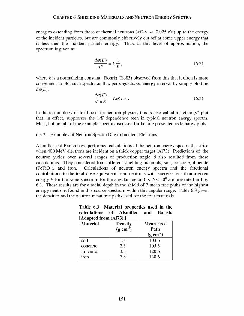
CHAPTER 6 SHIELDING MATERIALS AND NEUTRON ENERGY SPECTRA
151
energies extending from those of thermal neutrons (<En> ≈ 0.025 eV) up to the energy of the incident particles, but are commonly effectively cut off at some upper energy that is less then the incident particle energy. Thus, at this level of approximation, the spectrum is given as
d E
dEk
Eφ( )
=1
, (6.2)
where k is a normalizing constant. Rohrig (Ro83) observed from this that it often is more convenient to plot such spectra as flux per logarithmic energy interval by simply plotting Eφ(E);
d Ed E
E Eφ
φ( )
ln( )= . (6.3)
In the terminology of textbooks on neutron physics, this is also called a "lethargy" plot that, in effect, suppresses the 1/E dependence seen in typical neutron energy spectra. Most, but not all, of the example spectra discussed further are presented as lethargy plots. 6.3.2 Examples of Neutron Spectra Due to Incident Electrons Alsmiller and Barish have performed calculations of the neutron energy spectra that arise when 400 MeV electrons are incident on a thick copper target (Al73). Predictions of the neutron yields over several ranges of production angle θ also resulted from these calculations. They considered four different shielding materials; soil, concrete, ilmenite (FeTiO3), and iron. Calculations of neutron energy spectra and the fractional contributions to the total dose equivalent from neutrons with energies less than a given energy E for the same spectrum for the angular region 0 < θ < 30o are presented in Fig. 6.1. These results are for a radial depth in the shield of 7 mean free paths of the highest energy neutrons found in this source spectrum within this angular range. Table 6.3 gives the densities and the neutron mean free paths used for the four materials.
Table 6.3 Material properties used in the calculations of Alsmiller and Barish. [Adapted from (Al73).] Material Density
(g cm-3) Mean Free
Path (g cm-2)
soil 1.8 103.6 concrete 2.3 105.3 ilmenite 3.8 120.6 iron 7.8 138.6
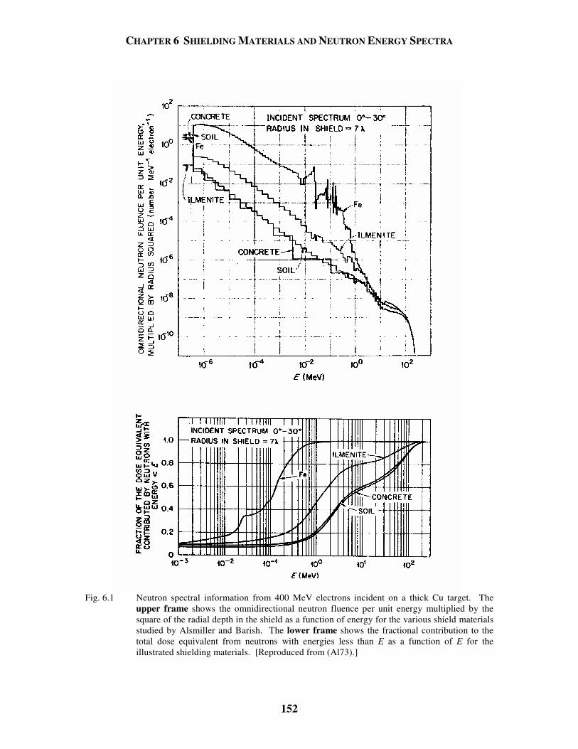
CHAPTER 6 SHIELDING MATERIALS AND NEUTRON ENERGY SPECTRA
152
Fig. 6.1 Neutron spectral information from 400 MeV electrons incident on a thick Cu target. The
upper frame shows the omnidirectional neutron fluence per unit energy multiplied by the square of the radial depth in the shield as a function of energy for the various shield materials studied by Alsmiller and Barish. The lower frame shows the fractional contribution to the total dose equivalent from neutrons with energies less than E as a function of E for the illustrated shielding materials. [Reproduced from (Al73).]
CHAPTER 6 SHIELDING MATERIALS AND NEUTRON ENERGY SPECTRA
153
In this figure, the inverse square dependence was removed to eliminate the effect of "geometrical" attenuation within the shield. It should be clear that the neutron spectra in the iron shield is markedly different from that found in the soil and concrete shields. The characteristics of the spectra found in the ilmenite are intermediate, perhaps related to the presence of iron in this material. The same kinds of phenomena associated with iron shielding are found in neutron energy spectra measured at high energy proton accelerators. Special considerations pertaining to neutron energy spectra emerging from iron shielding will be discussed in Section 6.3.5. 6.3.3 Examples of Neutron Spectra Due to Low and Intermediate Energy Protons Calculations and measurements of neutron energy spectra at various depths in shielding due to 52 MeV protons have been reported by Uwamino et al. (Uw82). These results are presented in Fig. 6.2. Alsmiller et al. (Al75) have provided predictions of neutron energy spectra averaged over specific angular intervals for 200 MeV protons stopped in a thick water target. The results are given for large angles are presented in Fig. 6.3. 6.3.4 Examples of Neutron Spectra Due to High Energy Protons In the regime of proton energies well above one GeV the details of the spectra are far more sensitive to geometrical considerations than they are dependent upon the incident proton energy. O'Brien carried out a calculation of a generalized neutron spectrum that could be found external to a high energy accelerator (OB71). These were compared with measurements and alternative calculations performed by Höfert and Stevenson (Hö84a). The results are provided in Fig. 6.4 for both "lateral" and "forward" angular regions. The results for forward angles also include the spectra of charged pions and protons. It is clear that at the forward angles, the total fluence of hadrons at high energies is likely to be a mixture of charged particles and neutrons. Detailed features of the geometry involved can produce peaks in the neutron energy spectrum. Examples of such spectra have been provided by various workers (Pa73, Th88, El86, McC88, and Co88). These peaks are typically encountered in the few MeV region. Figures 6.5, 6.6, 6.7, and 6.8 are plots of neutron spectra and sketches of the corresponding shielding geometry taken from Cossairt et al. (Co88). These spectra were obtained (i.e., "unfolded") using the Bonner sphere technique discussed in more detail in Section 9.5.2.1. In these four figures, “spheres” denote the locations where the neutron energy spectra were measured. These are typical of the spectra found at high energy proton accelerators. Figure 6.5 is rather typical of the spectra found external to earth and concrete shields lateral to high energy proton accelerators. The neutron energy spectrum displayed in Fig. 6.6 is particular interesting because its shape was demonstrated to be essentially independent of proton energy over the range of 150 to 900 GeV (McC88). Fig. 6.7 is typical of the results obtained in the second and succeeding sections (“legs”) of a labyrinth penetration.
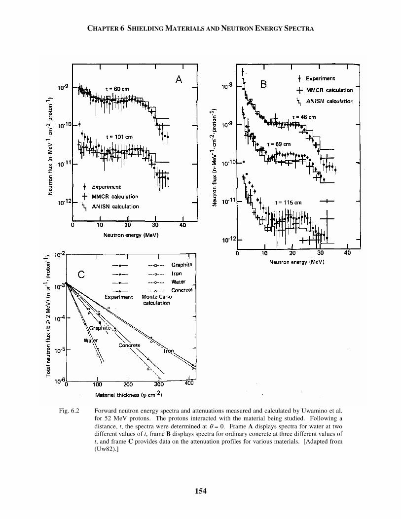
CHAPTER 6 SHIELDING MATERIALS AND NEUTRON ENERGY SPECTRA
154
Fig. 6.2 Forward neutron energy spectra and attenuations measured and calculated by Uwamino et al.
for 52 MeV protons. The protons interacted with the material being studied. Following a distance, t, the spectra were determined at θ = 0. Frame A displays spectra for water at two different values of t, frame B displays spectra for ordinary concrete at three different values of t, and frame C provides data on the attenuation profiles for various materials. [Adapted from (Uw82).]
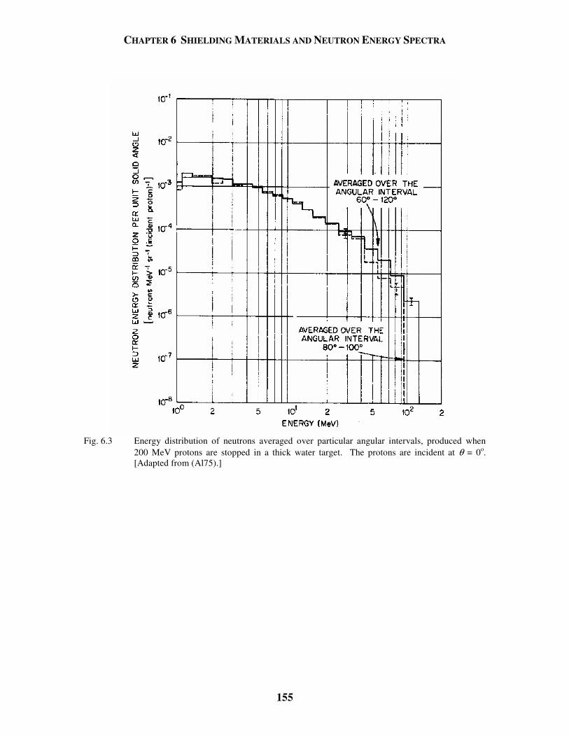
CHAPTER 6 SHIELDING MATERIALS AND NEUTRON ENERGY SPECTRA
155
Fig. 6.3 Energy distribution of neutrons averaged over particular angular intervals, produced when
200 MeV protons are stopped in a thick water target. The protons are incident at θ = 0o. [Adapted from (Al75).]
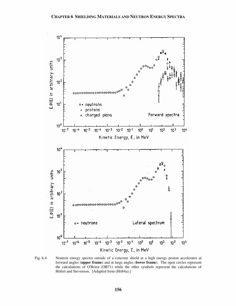
CHAPTER 6 SHIELDING MATERIALS AND NEUTRON ENERGY SPECTRA
156
Fig. 6.4 Neutron energy spectra outside of a concrete shield at a high energy proton accelerator at
forward angles (upper frame) and at large angles (lower frame). The open circles represent the calculations of O'Brien (OB71) while the other symbols represent the calculations of Höfert and Stevenson. [Adapted from (Hö84a).]
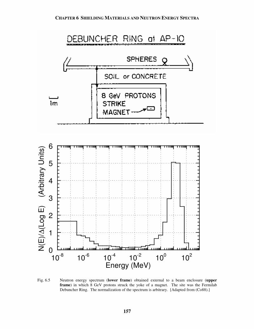
CHAPTER 6 SHIELDING MATERIALS AND NEUTRON ENERGY SPECTRA
157
0
1
2
3
4
5
6
10-8 10-6 10-4 10-2 100 102
N(E
)/∆(
Log
E)
(A
rbitr
ary
Uni
ts)
Energy (MeV)
Fig. 6.5 Neutron energy spectrum (lower frame) obtained external to a beam enclosure (upper
frame) in which 8 GeV protons struck the yoke of a magnet. The site was the Fermilab Debuncher Ring. The normalization of the spectrum is arbitrary. [Adapted from (Co88).]
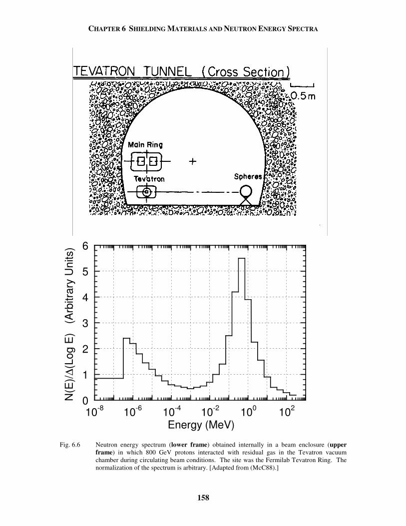
CHAPTER 6 SHIELDING MATERIALS AND NEUTRON ENERGY SPECTRA
158
0
1
2
3
4
5
6
10-8 10-6 10-4 10-2 100 102
N(E
)/∆(L
og E
) (A
rbitr
ary
Uni
ts)
Energy (MeV)
Fig. 6.6 Neutron energy spectrum (lower frame) obtained internally in a beam enclosure (upper
frame) in which 800 GeV protons interacted with residual gas in the Tevatron vacuum chamber during circulating beam conditions. The site was the Fermilab Tevatron Ring. The normalization of the spectrum is arbitrary. [Adapted from (McC88).]
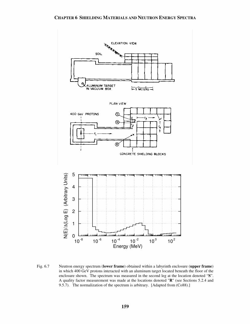
CHAPTER 6 SHIELDING MATERIALS AND NEUTRON ENERGY SPECTRA
159
0
1
2
3
4
5
10 -8 10 -6 10 -4 10 -2 10 0 10 2N(E
)/∆(
Log
E)
(Arb
itrar
y U
nits
)
Energy (MeV)
Fig. 6.7 Neutron energy spectrum (lower frame) obtained within a labyrinth enclosure (upper frame)
in which 400 GeV protons interacted with an aluminum target located beneath the floor of the enclosure shown. The spectrum was measured in the second leg at the location denoted “S”. A quality factor measurement was made at the locations denoted "R" (see Sections 5.2.4 and 9.5.7). The normalization of the spectrum is arbitrary. [Adapted from (Co88).]
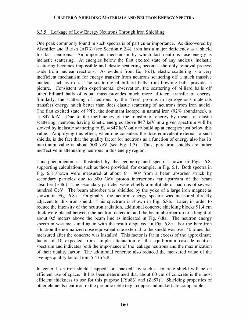
CHAPTER 6 SHIELDING MATERIALS AND NEUTRON ENERGY SPECTRA
160
6.3.5 Leakage of Low Energy Neutrons Through Iron Shielding One peak commonly found in such spectra is of particular importance. As discovered by Alsmiller and Barish (Al73) (see Section 6.2.4), iron has a major deficiency as a shield for fast neutrons. An important mechanism by which fast neutrons lose energy is inelastic scattering. At energies below the first excited state of any nucleus, inelastic scattering becomes impossible and elastic scattering becomes the only removal process aside from nuclear reactions. As evident from Eq. (6.1), elastic scattering is a very inefficient mechanism for energy transfer from neutrons scattering off a much massive nucleus such as iron. The scattering of billiard balls from bowling balls provides a picture. Consistent with experimental observation, the scattering of billiard balls off other billiard balls of equal mass provides much more efficient transfer of energy. Similarly, the scattering of neutrons by the "free" protons in hydrogenous materials transfers energy much better than does elastic scattering of neutrons from iron nuclei. The first excited state of 56Fe, the dominant isotope in natural iron (92% abundance), is at 847 keV. Due to the inefficiency of the transfer of energy by means of elastic scattering, neutrons having kinetic energies above 847 keV in a given spectrum will be slowed by inelastic scattering to En ≈ 847 keV only to build up at energies just below this value. Amplifying this effect, when one considers the dose equivalent external to such shields, is the fact that the quality factor for neutrons as a function of energy also has its maximum value at about 500 keV (see Fig. 1.3). Thus, pure iron shields are rather ineffective in attenuating neutrons in this energy region. This phenomenon is illustrated by the geometry and spectra shown in Figs. 6.8, supporting calculations such as those provided, for example, in Fig. 6.1. Both spectra in Fig. 6.8 shown were measured at about θ = 90o from a beam absorber struck by secondary particles due to 800 GeV proton interactions far upstream of the beam absorber (El86). The secondary particles were chiefly a multitude of hadrons of several hundred GeV. The beam absorber was shielded by the yoke of a large iron magnet as shown in Fig. 6.8a. Originally, the neutron energy spectra was measured directly adjacent to this iron shield. This spectrum is shown in Fig. 6.8b. Later, in order to reduce the intensity of the neutron radiation, additional concrete shielding blocks 91.4 cm thick were placed between the neutron detectors and the beam absorber up to a height of about 0.5 meters above the beam line as indicated in Fig. 6.8a. The neutron energy spectrum was measured again with the result displayed in Fig. 6.8c. For the bare iron situation the normalized dose equivalent rate external to the shield was over 40 times that measured after the concrete was installed. This factor is far in excess of the approximate factor of 10 expected from simple attenuation of the equilibrium cascade neutron spectrum and indicates both the importance of the leakage neutrons and the maximization of their quality factor. The additional concrete also reduced the measured value of the average quality factor from 5.4 to 2.8. In general, an iron shield "capped" or "backed" by such a concrete shield will be an efficient use of space. It has been determined that about 60 cm of concrete is the most efficient thickness to use for this purpose [(Yu83) and (Za87)]. Shielding properties of other elements near iron in the periodic table (e.g., copper and nickel) are comparable.
CHAPTER 6 SHIELDING MATERIALS AND NEUTRON ENERGY SPECTRA
161
Fig. 6.8a Situation for the measurements shown in Figs. 6.8b and 6.8c. A target far upstream (to the
left) of the apparatus shown in the figure was struck by 800 GeV protons. The beam axis was horizontal and 1.8 m above the floor. Secondary particles, largely hadrons, produced by these interactions were intercepted by the beam absorber shown in the Figure. The plain shielding blocks are of ordinary concrete. During initial operations, the cross-hatched blocks, also of ordinary concrete, were not in place between this beam absorber and the location of measurements and the result was the measured spectrum in Fig. 6.8b. Later, those blocks were added and the spectrum shown in Fig. 6.8c was measured. [Reproduced from (El86).]
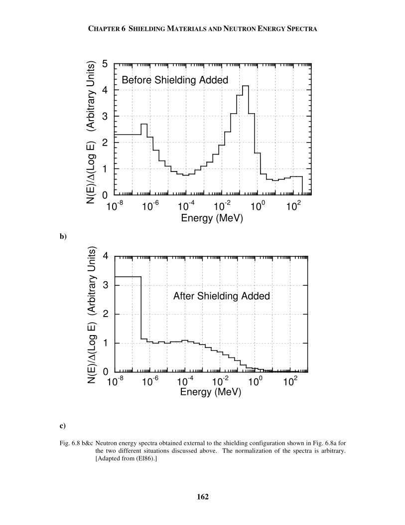
CHAPTER 6 SHIELDING MATERIALS AND NEUTRON ENERGY SPECTRA
162
0
1
2
3
4
5
10-8 10-6 10-4 10-2 100 102N(E
)/∆(L
og E
) (A
rbitr
ary
Uni
ts)
Energy (MeV)
Before Shielding Added
b)
0
1
2
3
4
10-8 10-6 10-4 10-2 100 102N(E
)/∆(L
og E
) (A
rbitr
ary
Uni
ts)
Energy (MeV)
After Shielding Added
c) Fig. 6.8 b&c Neutron energy spectra obtained external to the shielding configuration shown in Fig. 6.8a for
the two different situations discussed above. The normalization of the spectra is arbitrary. [Adapted from (El86).]
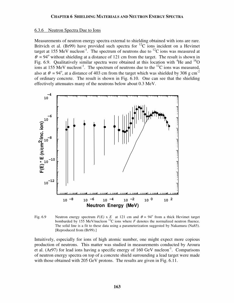
CHAPTER 6 SHIELDING MATERIALS AND NEUTRON ENERGY SPECTRA
163
6.3.6 Neutron Spectra Due to Ions Measurements of neutron energy spectra external to shielding obtained with ions are rare. Britvich et al. (Br99) have provided such spectra for 12C ions incident on a Hevimet target at 155 MeV nucleon-1. The spectrum of neutrons due to 12C ions was measured at θ = 94o without shielding at a distance of 121 cm from the target. The result is shown in Fig. 6.9. Qualitatively similar spectra were obtained at this location with 4He and 16O ions at 155 MeV nucleon-1. The spectrum of neutrons due to the 12C ions was measured, also at θ = 94o, at a distance of 403 cm from the target which was shielded by 308 g cm-2 of ordinary concrete. The result is shown in Fig. 6.10. One can see that the shielding effectively attenuates many of the neutrons below about 0.3 MeV.
10 210 010 -210 -410 -610 -8
10-12
10-10
10-8
10-6
10-4
Neutron Energy (MeV)
F(E
) * E
(n/c
m2 /
inc.
ion)
Fig. 6.9 Neutron energy spectrum F(E) x E at 121 cm and θ = 94o from a thick Hevimet target
bombarded by 155 MeV/nucleon 12C ions where F denotes the normalized neutron fluence. The solid line is a fit to these data using a parameterization suggested by Nakamura (Na85). [Reproduced from (Br99).]
Intuitively, especially for ions of high atomic number, one might expect more copious production of neutrons. This matter was studied in measurements conducted by Aroura et al. (Ar97) for lead ions having a specific energy of 160 GeV nucleon-1. Comparisons of neutron energy spectra on top of a concrete shield surrounding a lead target were made with those obtained with 205 GeV protons. The results are given in Fig. 6.11.
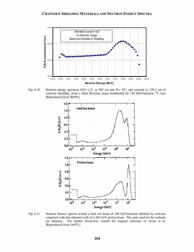
CHAPTER 6 SHIELDING MATERIALS AND NEUTRON ENERGY SPECTRA
164
1.E-15
1.E-14
1.E-13
1.E-12
1.E-09 1.E-08 1.E-07 1.E-06 1.E-05 1.E-04 1.E-03 1.E-02 1.E-01 1.E+00 1.E+01 1.E+02 1.E+03
Neutron Energy (MeV)
F(E
)*E
(neu
tro
ns/c
m2 /
ion
)
155 MeV/nucleon 12Con Hevimet target
Spectrum Outside of Shielding
Fig. 6.10 Neutron energy spectrum F(E) x E at 403 cm and θ = 94o, and external to 128.3 cm of
concrete shielding, from a thick Hevimet target bombarded by 155 MeV/nucleon 12C ions [Reproduced from (Br99)].
Fig. 6.11 Neutron fluence spectra around a lead ion beam of 160 GeV/nucleon shielded by concrete
compared with that obtained with of a 205 GeV proton beam. The units used for the ordinate are arbitrary. For further discussion, consult the original reference of Aroua et al. [Reproduced from (Ar97).]
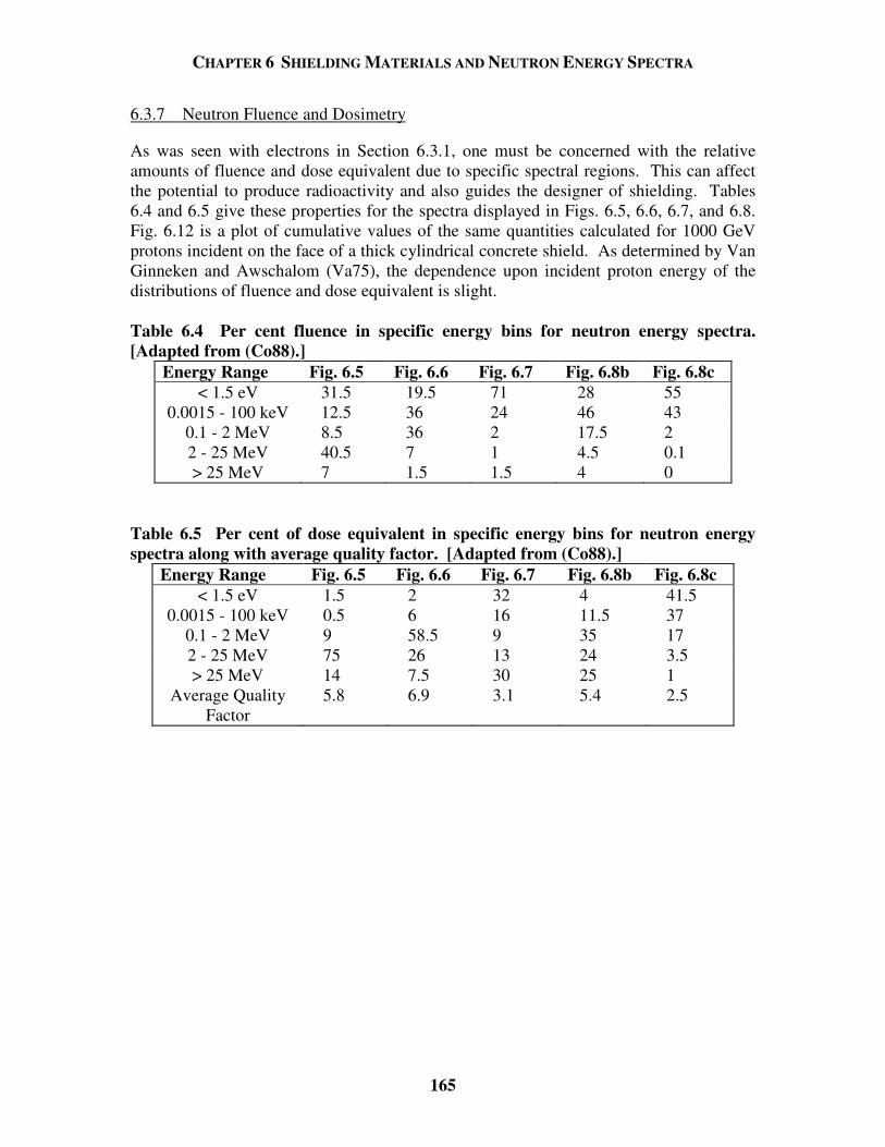
CHAPTER 6 SHIELDING MATERIALS AND NEUTRON ENERGY SPECTRA
165
6.3.7 Neutron Fluence and Dosimetry As was seen with electrons in Section 6.3.1, one must be concerned with the relative amounts of fluence and dose equivalent due to specific spectral regions. This can affect the potential to produce radioactivity and also guides the designer of shielding. Tables 6.4 and 6.5 give these properties for the spectra displayed in Figs. 6.5, 6.6, 6.7, and 6.8. Fig. 6.12 is a plot of cumulative values of the same quantities calculated for 1000 GeV protons incident on the face of a thick cylindrical concrete shield. As determined by Van Ginneken and Awschalom (Va75), the dependence upon incident proton energy of the distributions of fluence and dose equivalent is slight. Table 6.4 Per cent fluence in specific energy bins for neutron energy spectra. [Adapted from (Co88).]
Energy Range Fig. 6.5 Fig. 6.6 Fig. 6.7 Fig. 6.8b Fig. 6.8c < 1.5 eV 31.5 19.5 71 28 55
0.0015 - 100 keV 12.5 36 24 46 43 0.1 - 2 MeV 8.5 36 2 17.5 2 2 - 25 MeV 40.5 7 1 4.5 0.1 > 25 MeV 7 1.5 1.5 4 0
Table 6.5 Per cent of dose equivalent in specific energy bins for neutron energy spectra along with average quality factor. [Adapted from (Co88).]
Energy Range Fig. 6.5 Fig. 6.6 Fig. 6.7 Fig. 6.8b Fig. 6.8c < 1.5 eV 1.5 2 32 4 41.5
0.0015 - 100 keV 0.5 6 16 11.5 37 0.1 - 2 MeV 9 58.5 9 35 17 2 - 25 MeV 75 26 13 24 3.5 > 25 MeV 14 7.5 30 25 1
Average Quality Factor
5.8 6.9 3.1 5.4 2.5
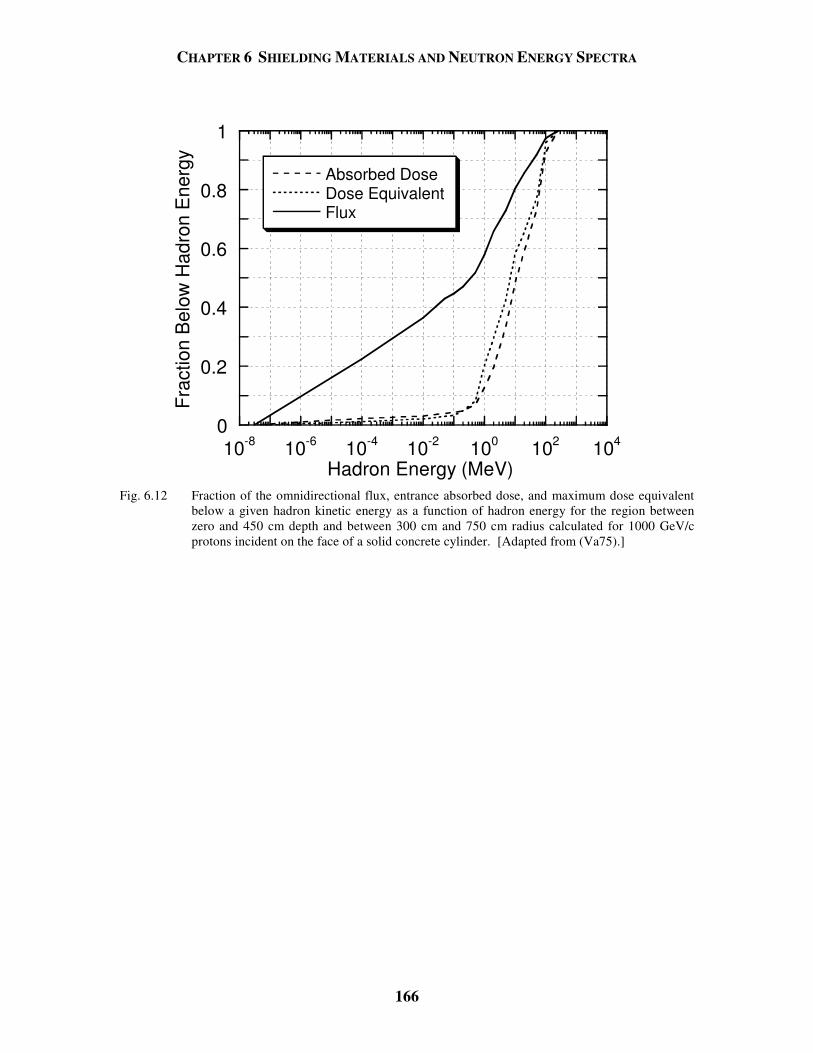
CHAPTER 6 SHIELDING MATERIALS AND NEUTRON ENERGY SPECTRA
166
0
0.2
0.4
0.6
0.8
1
10-8 10-6 10-4 10-2 100 102 104
Absorbed DoseDose EquivalentFlux
Frac
tion
Bel
ow H
adro
n E
nerg
y
Hadron Energy (MeV)
Fig. 6.12 Fraction of the omnidirectional flux, entrance absorbed dose, and maximum dose equivalent below a given hadron kinetic energy as a function of hadron energy for the region between zero and 450 cm depth and between 300 cm and 750 cm radius calculated for 1000 GeV/c protons incident on the face of a solid concrete cylinder. [Adapted from (Va75).]
CHAPTER 7 INDUCED RADIOACTIVITY IN ACCELERATOR COMPONENTS
167
7.1 Introduction In this chapter the production of induced radioactivity at accelerators is described. This discussion begins with a review of the basic principles of the production of radioactivity. It proceeds with a discussion of the activation of accelerator components including some generalizations that may be used for practical health physics applications. 7.2 Fundamental Principles of Induced Radioactivity In principle, induced radioactivity can be produced at all accelerators capable of liberating neutrons and other hadrons. When the accelerated beam strikes a nucleus, the resultant nuclear reactions can convert it into a different nuclide, which may or may not be radioactive. The activity of a given radionuclide refers to the number of atoms that decay per unit time. The customary unit of activity is the Curie (Ci), and its submultiples. One Curie was historically defined to be the activity of one gram of natural radium. It is now precisely defined as 3.7 x 10¹⁰ decays per second. The SI unit of activity is the Becquerel (Bq), which is defined to be 1 decay per second, with “multiples” such as Gbq commonly used. A related quantity of considerable importance is the specific activity that is defined to be the activity per unit volume (e.g., Bq cm-3) or, alternatively, the activity per unit mass (e.g., Bq g-1). Radioactive decay is a random process characterized by a mean-life (units of time) denoted by τ, and its reciprocal (units of inverse time), the decay constant14 λ, [λ = 1/τ ]. If a total of Ntot (t) atoms of a radionuclide are present at time t, the total activity Atot (t) is determined by the random nature of radioactive decay to be
( ) 1
( ) ( ) ( )tottot tot tot
dN tA t N t N t
dtλ
τ= − = = . (7.1)
If at time t = 0, Ntot (0) atoms are present, then this simple differential equation has the solution at some later time t = T, [with T > 0]; ( ) (0) exp( ) (0)exp( )tot tot totA T N T A Tλ λ λ= − = − . (7.2) Often, the time required to decay to half of the original activity, the half-life, t1/2, is tabulated and is related to the mean-life by the following:
τ = = =12
10 693
14421 2 1 2 1 2ln ../ / /t t t . (7.3)
In this text values of half-lives listed are from the National Nuclear Data Center (Tu05).
14Care needs to be taken with respect to the usage of the symbol λ. In the literature and in this text it is, at different points, used for both the attenuation length and for the decay constant. The reader needs to take note of the context to apply the correct meaning.
CHAPTER 7 INDUCED RADIOACTIVITY IN ACCELERATOR COMPONENTS
168
The most simple activation situation at accelerators is that of the steady irradiation of some material by a spatially uniform flux density of particles that begins at time t = 0 and continues at a constant rate for an irradiation period that ends at t = ti. This is followed by a decay period called the cooling time that is denoted tc, a period of time that begins at t = ti and ends at t = ti + tc. For this simple situation, self-absorption of the hadrons by the target is ignored, as is the fact that a whole spectrum of particles might be incident. Thus the process of producing the radioactivity is characterized by a single average cross section, σ . Ιn the more complicated generalized situations the value of this cross section must be obtained from averaging over the energy spectra of the particles incident. The number of atoms of the radionuclide of interest per unit volume will thus be governed by the following equation during the period of the irradiation:
dn t
dtn t N
( )( )= − +λ σφ , (7.4)
where n(t) is the number density of atoms of the radionuclide of interest at time t (cm-3), N is the number density of "target" atoms (cm-3), σ is the production cross section (cm2, and φ is the flux density (cm-2 sec-1) of incident particles. On the right hand side of the above equation, the first term represents the loss of radionuclides through decay during the irradiation while the second term represents the gain of radionuclides through the production reaction under consideration. The equation has the following solution for 0 < t < ti :
( )n tN t( ) = −
σφλ
λ1 e- . (7.5)
Thus the specific activity induced in the material as a function of time during the irradiation is given by a(t) = λ n(t), hence
( )a t N t( ) = −σφ λ1 e- (Bq cm-3) for 0 < t < ti. (7.6)
To obtain specific activity in units of Curies cm-3, one must simply divide the resulting value by the conversion factor 3.7 x 10¹⁰ Bq Curie-1. At the instant of completion of the irradiation (t = ti ), the specific activity will be given by
a t N ti i( ) exp( )= − −σφ λ1 (Bq cm-3), (7.7)
so that the specific activity as a function of time is characterized by a buildup from zero to the saturation concentration value of Nσφ for infinitely long irradiations. After the irradiation has ceased (t > ti ), the specific activity as a function of the cooling time, tc,
CHAPTER 7 INDUCED RADIOACTIVITY IN ACCELERATOR COMPONENTS
169
will obviously decay exponentially and be given by the activation equation; ( ) 1 exp( ) exp( )c i ca t N t tσφ λ λ= − − −
(Bq/cm3), (7.8)
where tc is the cooling time and tc = t - ti. (7.9) To obtain total activities in some object in situations where uniform flux densities of particles of constant energy are incident on a homogeneous "target", one can simply multiply by the volume of the "target". Or, in more complex cases involving non-uniform flux densities, one can integrate the above over the sub-volumes of the target. For γ-ray emitters typical of those emitted by accelerator-produced radionuclides in the range of from about 100 keV to 10 MeV, many textbooks in health physics demonstrate that the absorbed dose rate, dD/dt (rad h-1), at a distance r (meters) from a "point" source is approximately given in terms of the source strength, S, (Ci), and the photon energies present, Eγ i (MeV) by
20.4 i
i
dD SE
dt rγ= . (7.10)
The summation is over all γ-rays present, including appropriate branching fractions if multiple photons are emitted in the course of decay. If dD/dt is desired as an approximate absorbed dose rate in Gy h-1 at a distance, r (meters), from a source strength S in gigaBecquerels15 (GBq), the constant 0.4 becomes 1.08 x 10⁻⁴. One can use the above to determine the absorbed dose rate from a given activated object if it is a point source. For non-point sources, an appropriate spatial integration must be performed. 7.3 Activation of Components at Electron Accelerators 7.3.1 General Phenomena At electron accelerators, as was described in Chapter 3, the direct interactions of electrons in material results in the copious production of photons. Through various nuclear reaction channels, these photons then proceed to produce charged particles and neutrons that then interact further with material to produce radioactivity. In general, if the facility is properly shielded against prompt radiation, the radioactivity hazard will be confined to accelerator components and the interior of the accelerator enclosure. The experience at most accelerators bears this out. The vast majority of the radiation exposure incurred by the workers is due to maintenance activities on radioactivated components, handling and moving of activated items, radiation surveys, and radioactive waste handling rather than to exposure to the prompt radiation fields. An understanding of the production of radionuclides can help reduce personnel exposures through the selection of more appropriate machine component materials and the optimization of
15The GBq (109Bq) or MBq (106) are often better units of activity for practical work than is the tiny Bq.
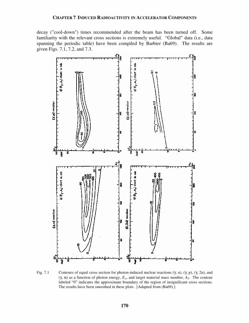
CHAPTER 7 INDUCED RADIOACTIVITY IN ACCELERATOR COMPONENTS
170
decay ("cool-down") times recommended after the beam has been turned off. Some familiarity with the relevant cross sections is extremely useful. “Global” data (i.e., data spanning the periodic table) have been compiled by Barbier (Ba69). The results are given Figs. 7.1, 7.2, and 7.3.
Fig. 7.1 Contours of equal cross section for photon-induced nuclear reactions (γ, n), (γ, p), (γ, 2n), and (γ, α) as a function of photon energy, Eγ , and target material mass number, AT. The coutour labeled “0” indicates the approximate boundary of the region of insignificant cross sections. The results have been smoothed in these plots. [Adapted from (Ba69).]
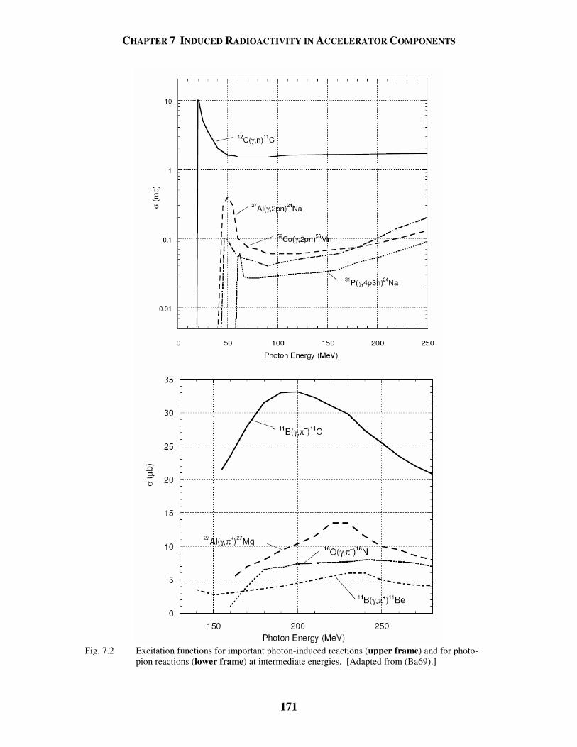
CHAPTER 7 INDUCED RADIOACTIVITY IN ACCELERATOR COMPONENTS
171
Fig. 7.2 Excitation functions for important photon-induced reactions (upper frame) and for photo-
pion reactions (lower frame) at intermediate energies. [Adapted from (Ba69).]
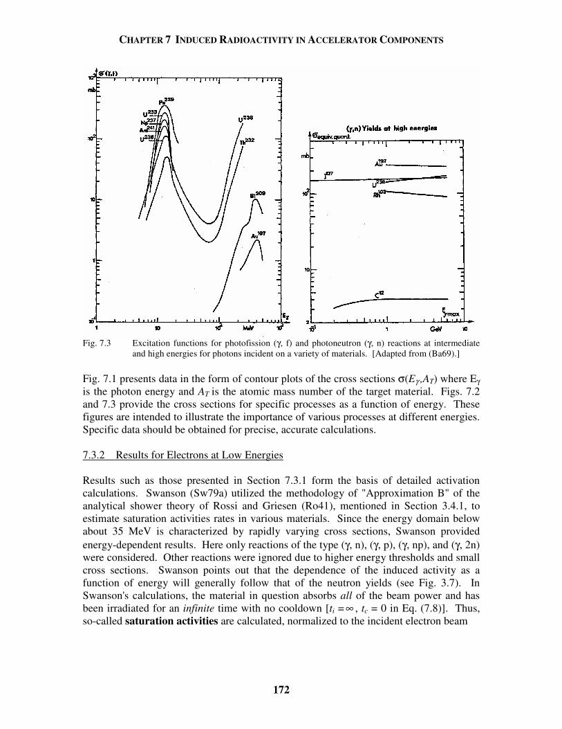
CHAPTER 7 INDUCED RADIOACTIVITY IN ACCELERATOR COMPONENTS
172
Fig. 7.3 Excitation functions for photofission (γ, f) and photoneutron (γ, n) reactions at intermediate
and high energies for photons incident on a variety of materials. [Adapted from (Ba69).] Fig. 7.1 presents data in the form of contour plots of the cross sections σ(Eγ ,AT) where Eγ is the photon energy and AT is the atomic mass number of the target material. Figs. 7.2 and 7.3 provide the cross sections for specific processes as a function of energy. These figures are intended to illustrate the importance of various processes at different energies. Specific data should be obtained for precise, accurate calculations. 7.3.2 Results for Electrons at Low Energies Results such as those presented in Section 7.3.1 form the basis of detailed activation calculations. Swanson (Sw79a) utilized the methodology of "Approximation B" of the analytical shower theory of Rossi and Griesen (Ro41), mentioned in Section 3.4.1, to estimate saturation activities rates in various materials. Since the energy domain below about 35 MeV is characterized by rapidly varying cross sections, Swanson provided energy-dependent results. Here only reactions of the type (γ, n), (γ, p), (γ, np), and (γ, 2n) were considered. Other reactions were ignored due to higher energy thresholds and small cross sections. Swanson points out that the dependence of the induced activity as a function of energy will generally follow that of the neutron yields (see Fig. 3.7). In Swanson's calculations, the material in question absorbs all of the beam power and has been irradiated for an infinite time with no cooldown [ti = ∞ , tc = 0 in Eq. (7.8)]. Thus, so-called saturation activities are calculated, normalized to the incident electron beam
CHAPTER 7 INDUCED RADIOACTIVITY IN ACCELERATOR COMPONENTS
173
power (kW). Results of these calculations, taking into account the natural isotopic abundances and reaction thresholds, are provided in Table 7.1. The results are probably accurate to about + 30 per cent. At these low energies, the distribution of the radioactivity can often approximately be taken to be that of a point source for calculating the residual absorbed dose rates using, for example, Eq. (7.10), taking the summation over all of the γ-ray emitters presented at a given time. Table 7.1 provides the specific gamma-ray constant, Γ, for each tabulated radionuclide. These constants connect activity with the absorbed dose rates at a distance of one meter for point source conditions accounting for all the photons emitted by the decaying radionuclide and including those emitted secondarily such as internal bremsstrahlung and annihilation radiation due to β+ emission manifested in the form of a pair of 0.511 MeV photons. For point sources, absorbed dose rates at other distances can be calculated by incorporating the inverse square law. In this context, absorbed dose rate is “loosely” connected with a somewhat obsolete unit, the exposure rate (R h-1). Exposure rate is tied to the rate of liberation of ions in air by photons and is only defined for photon radiation fields. The quantity one R h-1 is the hourly liberation of one electrostatic unit of charge cm-3 of air at STP [1 R = 2.58 x 10⁻⁴ Coulomb kg-1]. An exposure rate of 1.0 R h-1 is approximately equal to 0.95 rad h-1 of absorbed dose rate in tissue placed in the radiation field under consideration.
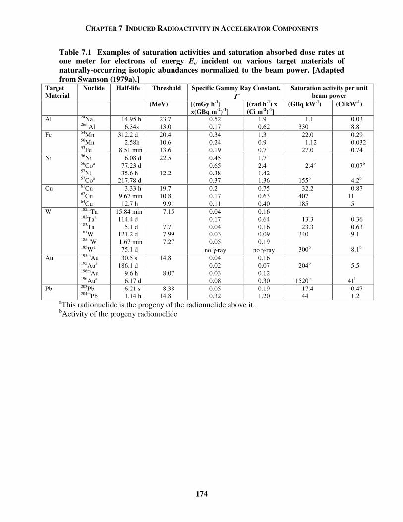
CHAPTER 7 INDUCED RADIOACTIVITY IN ACCELERATOR COMPONENTS
174
Table 7.1 Examples of saturation activities and saturation absorbed dose rates at one meter for electrons of energy Eo incident on various target materials of naturally-occurring isotopic abundances normalized to the beam power. [Adapted from Swanson (1979a).]
Target Material
Nuclide Half-life Threshold Specific Gammy Ray Constant, ΓΓΓΓ
Saturation activity per unit beam power
(MeV) [(mGy h-1) x(GBq m-2)-1]
[(rad h-1) x (Ci m-2)-1]
(GBq kW-1) (Ci kW-1)
Al 24Na 14.95 h 23.7 0.52 1.9 1.1 0.03 26mAl 6.34s 13.0 0.17 0.62 330 8.8 Fe 54Mn 312.2 d 20.4 0.34 1.3 22.0 0.29 56Mn 2.58h 10.6 0.24 0.9 1.12 0.032 53Fe 8.51 min 13.6 0.19 0.7 27.0 0.74 Ni 56Ni 6.08 d 22.5 0.45 1.7 56Coa 77.23 d 0.65 2.4 2.4b 0.07b
57Ni 35.6 h 12.2 0.38 1.42 57Coa 217.78 d 0.37 1.36 155b 4.2b
Cu 61Cu 3.33 h 19.7 0.2 0.75 32.2 0.87 62Cu 9.67 min 10.8 0.17 0.63 407 11 64Cu 12.7 h 9.91 0.11 0.40 185 5 W 182mTa 15.84 min 7.15 0.04 0.16 182Taa 114.4 d 0.17 0.64 13.3 0.36 183Ta 5.1 d 7.71 0.04 0.16 23.3 0.63 181W 121.2 d 7.99 0.03 0.09 340 9.1 185mW 1.67 min 7.27 0.05 0.19 185Wa 75.1 d no γ-ray no γ-ray 300b 8.1b
Au 195mAu 30.5 s 14.8 0.04 0.16 195Aua 186.1 d 0.02 0.07 204b 5.5 196mAu 9.6 h 8.07 0.03 0.12 196Aua 6.17 d 0.08 0.30 1520b 41b
Pb 203Pb 6.21 s 8.38 0.05 0.19 17.4 0.47 204mPb 1.14 h 14.8 0.32 1.20 44 1.2
aThis radionuclide is the progeny of the radionuclide above it. bActivity of the progeny radionuclide
CHAPTER 7 INDUCED RADIOACTIVITY IN ACCELERATOR COMPONENTS
175
7.3.3 Results for Electrons at High Energies For higher energy electrons, more reaction channels become available but the energy dependence is diminished. Swanson has also performed calculations of the production of radionuclides in this energy domain and the results are provided here in Table 7.2 (Sw79a). The results are valid to within an approximate factor of two for any beam energy Eo that is somewhat above the nuclide production threshold. Specific gamma-ray constants for point source conditions, Γ, reaction thresholds, and integral radionuclide production cross sections summed over parent isotopes per MeV of electron beam energy, denoted by the somewhat esoteric symbol 2fσ −Σ , are provided along with saturation activities and exposures rates. This quantity is a useful one because of the dominance, and lack of energy dependence, of the photoneutron production process, as was discussed in Section 3.2. The electrons are assumed to be totally absorbed in the material and no self-shielding effects are taken into account. The distribution of radioactivity within the material is not taken into account. The results are, again, presented for saturation conditions, i.e. ti = ∞ , tc = 0 in Eq. (7.8), for the compositions of materials described in the footnotes to the table. Cooling curves have been reported by Barbier (Ba69) for high energy electrons incident on various materials for an infinite irradiation at the rate of one electron per second. The results are given in Fig. 7.4, again per MeV of incident electron energy, for an infinite irradiation time, ti. In this figure, results are given for the absorbed dose rates (mGy hr-1) per electron s-1 assuming the applicability of point source conditions. As discussed in Chapter 3, the lack of strong energy dependence (i.e., the scaling with incident beam power) and the simplicity of the photoneutron spectra make possible these rather uncomplicated results.
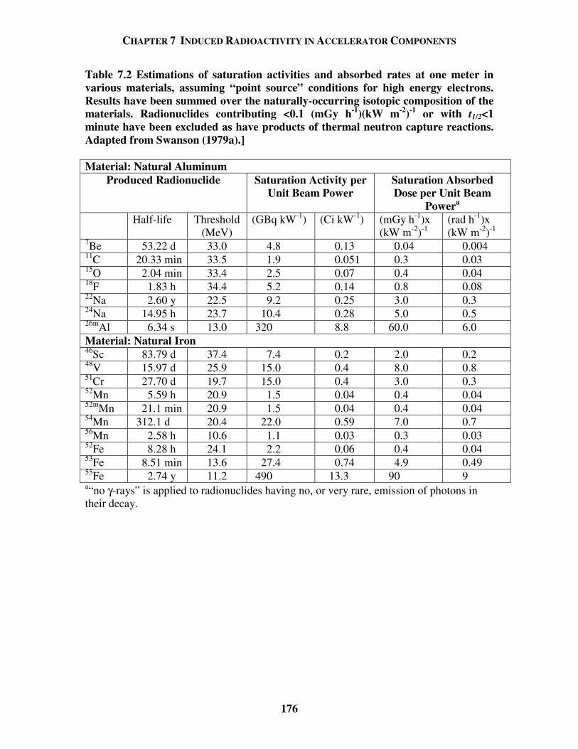
CHAPTER 7 INDUCED RADIOACTIVITY IN ACCELERATOR COMPONENTS
176
Table 7.2 Estimations of saturation activities and absorbed rates at one meter in various materials, assuming “point source” conditions for high energy electrons. Results have been summed over the naturally-occurring isotopic composition of the materials. Radionuclides contributing <0.1 (mGy h-1)(kW m-2)-1 or with t1/2<1 minute have been excluded as have products of thermal neutron capture reactions. Adapted from Swanson (1979a).] Material: Natural Aluminum
Produced Radionuclide Saturation Activity per Unit Beam Power
Saturation Absorbed Dose per Unit Beam
Powera
Half-life Threshold (MeV)
(GBq kW-1) (Ci kW-1) (mGy h-1)x (kW m-2)-1
(rad h-1)x (kW m-2)-1
7Be 53.22 d 33.0 4.8 0.13 0.04 0.004 11C 20.33 min 33.5 1.9 0.051 0.3 0.03 15O 2.04 min 33.4 2.5 0.07 0.4 0.04 18F 1.83 h 34.4 5.2 0.14 0.8 0.08 22Na 2.60 y 22.5 9.2 0.25 3.0 0.3 24Na 14.95 h 23.7 10.4 0.28 5.0 0.5 26mAl 6.34 s 13.0 320 8.8 60.0 6.0 Material: Natural Iron 46Sc 83.79 d 37.4 7.4 0.2 2.0 0.2 48V 15.97 d 25.9 15.0 0.4 8.0 0.8 51Cr 27.70 d 19.7 15.0 0.4 3.0 0.3 52Mn 5.59 h 20.9 1.5 0.04 0.4 0.04 52mMn 21.1 min 20.9 1.5 0.04 0.4 0.04 54Mn 312.1 d 20.4 22.0 0.59 7.0 0.7 56Mn 2.58 h 10.6 1.1 0.03 0.3 0.03 52Fe 8.28 h 24.1 2.2 0.06 0.4 0.04 53Fe 8.51 min 13.6 27.4 0.74 4.9 0.49 55Fe 2.74 y 11.2 490 13.3 90 9 a“no γ-rays” is applied to radionuclides having no, or very rare, emission of photons in their decay.
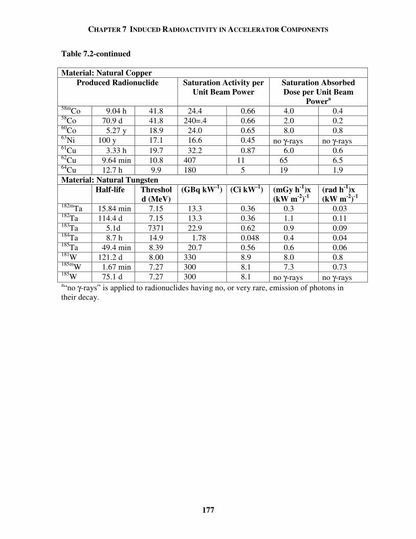
CHAPTER 7 INDUCED RADIOACTIVITY IN ACCELERATOR COMPONENTS
177
Table 7.2-continued
Material: Natural Copper Produced Radionuclide Saturation Activity per
Unit Beam Power Saturation Absorbed Dose per Unit Beam
Powera
58mCo 9.04 h 41.8 24.4 0.66 4.0 0.4 58Co 70.9 d 41.8 240=.4 0.66 2.0 0.2 60Co 5.27 y 18.9 24.0 0.65 8.0 0.8 63Ni 100 y 17.1 16.6 0.45 no γ-rays no γ-rays 61Cu 3.33 h 19.7 32.2 0.87 6.0 0.6 62Cu 9.64 min 10.8 407 11 65 6.5 64Cu 12.7 h 9.9 180 5 19 1.9 Material: Natural Tungsten Half-life Threshol
d (MeV) (GBq kW-1) (Ci kW-1) (mGy h-1)x
(kW m-2)-1 (rad h-1)x (kW m-2)-1
182mTa 15.84 min 7.15 13.3 0.36 0.3 0.03 182Ta 114.4 d 7.15 13.3 0.36 1.1 0.11 183Ta 5.1d 7371 22.9 0.62 0.9 0.09 184Ta 8.7 h 14.9 1.78 0.048 0.4 0.04 185Ta 49.4 min 8.39 20.7 0.56 0.6 0.06 181W 121.2 d 8.00 330 8.9 8.0 0.8 185mW 1.67 min 7.27 300 8.1 7.3 0.73 185W 75.1 d 7.27 300 8.1 no γ-rays no γ-rays a“no γ-rays” is applied to radionuclides having no, or very rare, emission of photons in their decay.
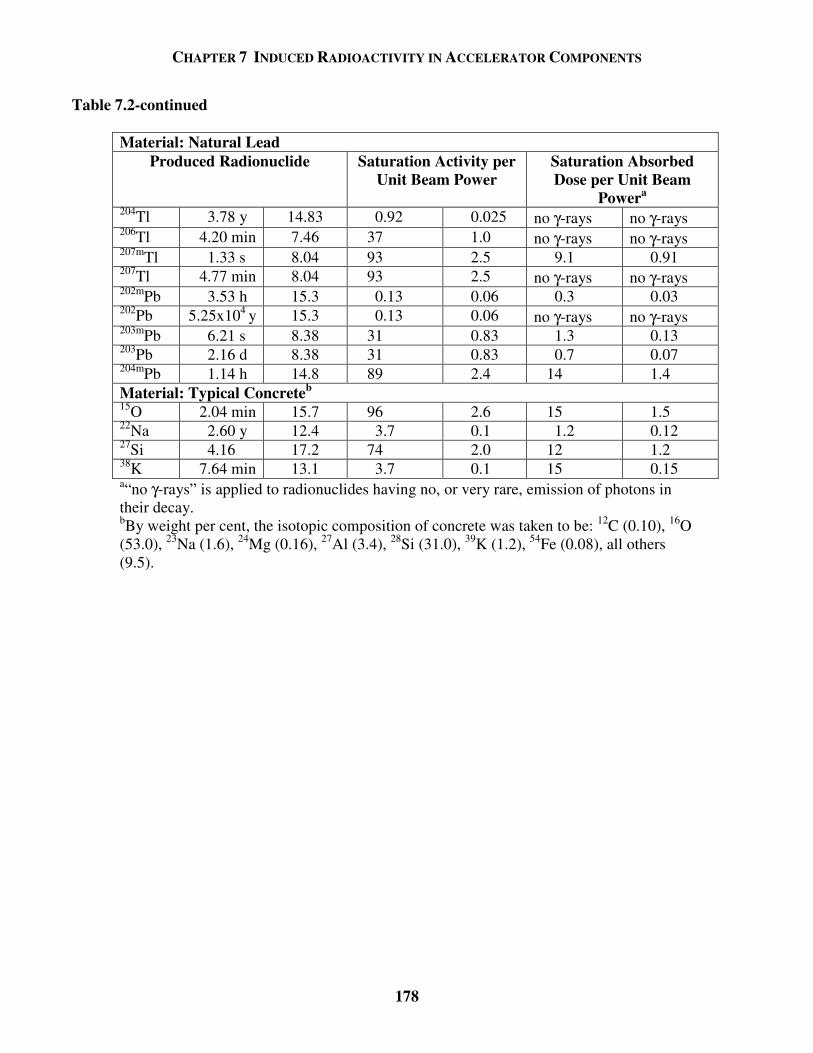
CHAPTER 7 INDUCED RADIOACTIVITY IN ACCELERATOR COMPONENTS
178
Table 7.2-continued
Material: Natural Lead Produced Radionuclide Saturation Activity per
Unit Beam Power Saturation Absorbed Dose per Unit Beam
Powera
204Tl 3.78 y 14.83 0.92 0.025 no γ-rays no γ-rays 206Tl 4.20 min 7.46 37 1.0 no γ-rays no γ-rays 207mTl 1.33 s 8.04 93 2.5 9.1 0.91 207Tl 4.77 min 8.04 93 2.5 no γ-rays no γ-rays 202mPb 3.53 h 15.3 0.13 0.06 0.3 0.03 202Pb 5.25x10⁴ y 15.3 0.13 0.06 no γ-rays no γ-rays 203mPb 6.21 s 8.38 31 0.83 1.3 0.13 203Pb 2.16 d 8.38 31 0.83 0.7 0.07 204mPb 1.14 h 14.8 89 2.4 14 1.4 Material: Typical Concreteb
15O 2.04 min 15.7 96 2.6 15 1.5 22Na 2.60 y 12.4 3.7 0.1 1.2 0.12 27Si 4.16 17.2 74 2.0 12 1.2 38K 7.64 min 13.1 3.7 0.1 15 0.15 a“no γ-rays” is applied to radionuclides having no, or very rare, emission of photons in their decay. bBy weight per cent, the isotopic composition of concrete was taken to be: 12C (0.10), 16O (53.0), 23Na (1.6), 24Mg (0.16), 27Al (3.4), 28Si (31.0), 39K (1.2), 54Fe (0.08), all others (9.5).
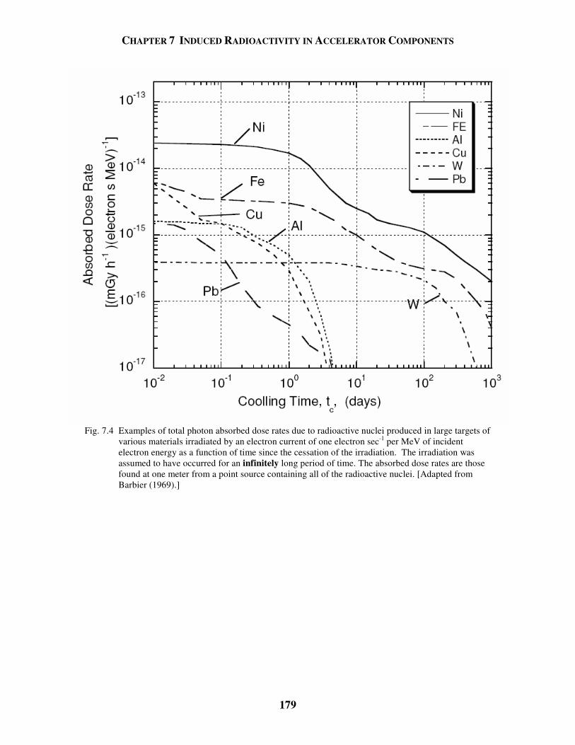
CHAPTER 7 INDUCED RADIOACTIVITY IN ACCELERATOR COMPONENTS
179
Fig. 7.4 Examples of total photon absorbed dose rates due to radioactive nuclei produced in large targets of
various materials irradiated by an electron current of one electron sec-1 per MeV of incident electron energy as a function of time since the cessation of the irradiation. The irradiation was assumed to have occurred for an infinitely long period of time. The absorbed dose rates are those found at one meter from a point source containing all of the radioactive nuclei. [Adapted from Barbier (1969).]
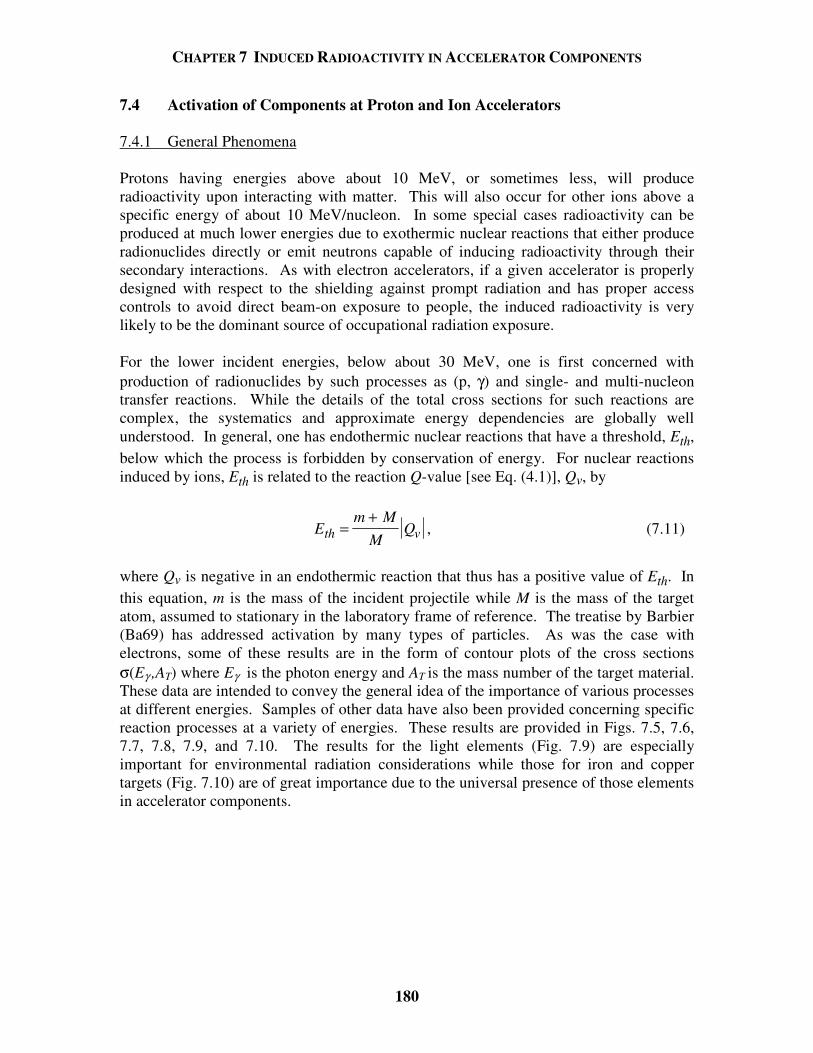
CHAPTER 7 INDUCED RADIOACTIVITY IN ACCELERATOR COMPONENTS
180
7.4 Activation of Components at Proton and Ion Accelerators 7.4.1 General Phenomena Protons having energies above about 10 MeV, or sometimes less, will produce radioactivity upon interacting with matter. This will also occur for other ions above a specific energy of about 10 MeV/nucleon. In some special cases radioactivity can be produced at much lower energies due to exothermic nuclear reactions that either produce radionuclides directly or emit neutrons capable of inducing radioactivity through their secondary interactions. As with electron accelerators, if a given accelerator is properly designed with respect to the shielding against prompt radiation and has proper access controls to avoid direct beam-on exposure to people, the induced radioactivity is very likely to be the dominant source of occupational radiation exposure. For the lower incident energies, below about 30 MeV, one is first concerned with production of radionuclides by such processes as (p, γ) and single- and multi-nucleon transfer reactions. While the details of the total cross sections for such reactions are complex, the systematics and approximate energy dependencies are globally well understood. In general, one has endothermic nuclear reactions that have a threshold, Eth, below which the process is forbidden by conservation of energy. For nuclear reactions induced by ions, Eth is related to the reaction Q-value [see Eq. (4.1)], Qv, by
Em M
MQth v=
+, (7.11)
where Qv is negative in an endothermic reaction that thus has a positive value of Eth. In this equation, m is the mass of the incident projectile while M is the mass of the target atom, assumed to stationary in the laboratory frame of reference. The treatise by Barbier (Ba69) has addressed activation by many types of particles. As was the case with electrons, some of these results are in the form of contour plots of the cross sections σ(Eγ ,AT) where Eγ is the photon energy and AT is the mass number of the target material. These data are intended to convey the general idea of the importance of various processes at different energies. Samples of other data have also been provided concerning specific reaction processes at a variety of energies. These results are provided in Figs. 7.5, 7.6, 7.7, 7.8, 7.9, and 7.10. The results for the light elements (Fig. 7.9) are especially important for environmental radiation considerations while those for iron and copper targets (Fig. 7.10) are of great importance due to the universal presence of those elements in accelerator components.
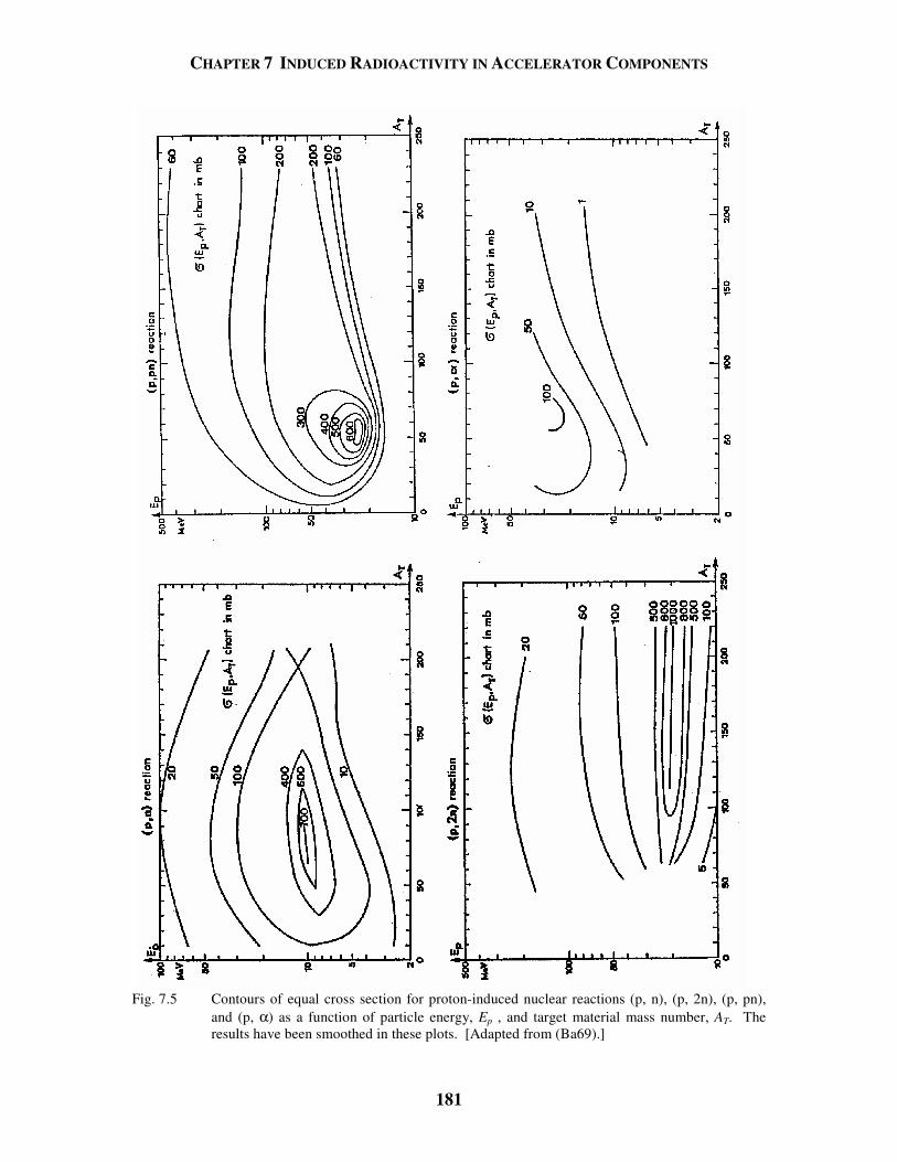
CHAPTER 7 INDUCED RADIOACTIVITY IN ACCELERATOR COMPONENTS
181
Fig. 7.5 Contours of equal cross section for proton-induced nuclear reactions (p, n), (p, 2n), (p, pn),
and (p, α) as a function of particle energy, Ep , and target material mass number, AT. The results have been smoothed in these plots. [Adapted from (Ba69).]
CHAPTER 7 INDUCED RADIOACTIVITY IN ACCELERATOR COMPONENTS
182
Fig. 7.6 Contours of equal cross section for neutron-induced nuclear reactions (n, p), (n, 2n), and (n,
α) as a function of particle energy, En , and target material mass number, AT. The results have been smoothed in these plots. [Adapted from (Ba69).]
CHAPTER 7 INDUCED RADIOACTIVITY IN ACCELERATOR COMPONENTS
183
Fig. 7.7 Contours of equal cross section for deuteron-induced nuclear reactions (d, n), (d, 2n), (d, p),
and (d, α) as a function of particle energy, Ed , and target material mass number, AT. The results have been smoothed in these plots. [Adapted from (Ba69).]
CHAPTER 7 INDUCED RADIOACTIVITY IN ACCELERATOR COMPONENTS
184
Fig. 7.8 Contours of equal cross section for α-particle-induced nuclear reactions (α, n), (α, 2n), (α, p),
and (α, pn) as a function of particle energy, Eα , and target material mass number, AT. The results have been smoothed in these plots. [Adapted from (Ba69).]
CHAPTER 7 INDUCED RADIOACTIVITY IN ACCELERATOR COMPONENTS
185
Fig. 7.9 Excitation functions for the production of various radionuclides by protons incident on some
light targets. [Reproduced from (Ba69).]
CHAPTER 7 INDUCED RADIOACTIVITY IN ACCELERATOR COMPONENTS
186
Fig. 7.10 Excitation functions for the production of various radionuclides by protons incident on iron
and copper targets. [Reproduced from (Ba69).] Thick target yields of radionuclides for targets having a range of atomic numbers have been systematically studied by Cohen for a number of nuclear processes spanning the periodic table (Co78). Fig. 7.11 is a representative plot of the general features of such excitation functions of such nuclear reactions. Specific processes may vary considerably from this behavior since “resonances” at specific nuclear excited states have been ignored. Table 7.3 lists a variety of such nuclear reactions along with the range of values of energy above threshold at which the radioactivity production rate has risen to 0.1% of the saturation value and also the range of saturation values for the production of radioactivity. It is assumed that the target thickness comfortably exceeds the range of the incident ion and that the irradiation period greatly exceeds the half-life of the radionuclide of interest. For shorter bombarding periods, ti, one needs to multiply by the factor [1 - exp(-λti) ]. Over the energy range of these curves, the importance of activation by secondary particles is small compared to that encountered at higher energies.
CHAPTER 7 INDUCED RADIOACTIVITY IN ACCELERATOR COMPONENTS
187
10-3
10-2
10-1
100
0 5 10 15 20 25 30
Frac
tion
of S
atur
ated
R
adio
nucl
ide
Yie
ld
E-Eth (MeV)
Fig. 7.11 Typical behavior of radionuclide production by (p, γ) or few-nucleon transfer reactions for
energies not far above the reaction threshold, Eth. This behavior is typical of the nuclear reactions tabulated in Table 7.3. For detailed calculations, data related to specific reactions on specific target materials should be used. [Adapted from (Co78).]
Table 7.3 Tabulation of generalized parameters for the production of radionuclides by means of low energy nuclear reactions which span the periodic table. The ranges of energies are listed at which the production yields are at approximately 0.1 per cent of the tabulated saturation values. The "high/low" values for the saturated activity are also given. [Adapted from (Co78).] Reaction 0.1%
Yield-low (E-Eth) (MeV)
0.1% Yield-high (E-Eth) (MeV)
Sat. Yield-low (µµµµCi/ µµµµA)
Sat. Yield-high (µµµµCi/ µµµµA)
Reaction 0.1% Yield-low (E-Eth) (MeV)
0.1% Yield-high (E-Eth) (MeV)
Sat. Yield-low (µµµµCi/ µµµµA)
Sat. Yield-high (µµµµCi/ µµµµA)
(p,γ) 4 9 3 x 10² 103 (3He,γ) 4 6 1 2 (p,n) 0 6 3 x 10⁵ 8 x 10⁵ (3He,n) 3 12 102 3 x 10² (p,2n) 1 4 3 x 10⁵ 106 (3He,2n) 2 7 3 x 10² 4 x 10³ (p,3n) 1 6 3 x 10⁵ 106 (3He,3n) 2 5 2 x 10³ 3 x 10⁴ (p,4n) 5 8 2 x 10⁵ 106 (3He,2p) 4 12 2 x 10² 104 (p,5n) 5 10 105 2 x 10⁶ (3He,α) 6 14 2 x 10² 103 (p,pn) 2 5 2 x 10⁵ 2 x 10⁶ (3He,p3n) 10 15 104 4 x 10⁵ (p,p2n) 3 8 3 x 10⁵ 2 x 10⁶ (α,γ) 10 13 3 20 (d,γ) 5 7 30 100 (α,n) 1 9 3 x 10² 104 (d,n) 2 7 4 x 10³ 3 x 10⁵ (α,2n) 1 4 5 x 10³ 4 x 10⁴ (d,2n) 2 5 2 x 10⁵ 6 x 10⁶ (α,3n) 1 6 3 x 10³ 7 x 10⁵ (d,3n) 1 4 3 x 10⁵ 106 (α,4n) 5 8 3 x 10³ 4 x 10⁴ (d,4n) 4 8 2 x 10⁵ 6 x 10⁵ (α,5n) 5 8 104 3 x 10⁵ (d,5n) 6 10 105 106 (α,p) 5 8 6 x 10² 2 x 10⁴ (d,p) 2 7 4 x 10⁴ 3 x 10⁵ (α,pn) 3 12 3 x 10³ 8 x 10⁴ (d,p2n) 2 10 105 2 x 10⁶ (α,p2n) 5 15 3 x 10³ 7 x 10⁴ (d,p3n) 8 15 105 2 x 10⁶ (α,p3n) 7 15 104 3 x 10⁴ (d,2p) 5 15 3 x 10³ 4 x 10⁴ (α,2p) 5 10 102 3 x 10³ (d,α) 4 7 104 3 x 10⁴ (α,αn) 6 16 3 x 10³ 3 x 10⁴ (d,αn) 5 15 2 x 10⁴ 105
CHAPTER 7 INDUCED RADIOACTIVITY IN ACCELERATOR COMPONENTS
188
7.4.2 Methods of Systematizing Activation Due to High Energy Hadrons For proton and ion accelerators of higher energy, the neglect of secondary reactions and the restriction to few- and multi-nucleon transfer reactions can become a serious deficiency in the accuracy of estimation of induced radioactivity because of the rise in importance of such processes as spallation. Below a kinetic energy of about 40 MeV only few-nucleon transfer reactions are available. The variety of radionuclides that can be produced increases as one increases the bombarding energy because more thresholds are exceeded. As a general rule, at high energies (Eo ≈ 1 GeV or greater), one must consider that all radionuclides in the periodic table that have mass numbers less than that of the material exposed to the flux of hadrons may be produced. Of course, many of these are of little significance due to short lifetimes and small production cross sections. In fact, the cross sections for producing specific radionuclides often are nearly independent of the target element. Table 7.4 gives a list radionuclides typically encountered in high energy proton accelerator installations and their half-lives. In this table only nuclides with half-lives between 10 minutes and 5 years are listed. Also, all "pure" β- (electron) emitters are ignored. Pure β− emitters are those radionuclides that emit no γ-rays in their decays. Pure β- emitters generally present minimal exposure hazards at accelerators as compared with γ-ray emitters in routine maintenance activities since the radionuclides are produced throughout the materials comprising accelerator components, with resultant self-shielding of most of the electrons compared with the less effective shielding of the more penetrating γ-rays. In contrast, β+ (positron) emitters are included in this table due to the generation of the pairs of 0.511 MeV photons that result from annihilation of the positrons with electrons in matter. Approximate thresholds and high energy cross sections for production of these radionuclides by protons, generally taken from the treatise by Barbier (Ba69), are also provided where available. A systematic way of addressing the great multiplicity of radionuclides produced in accelerator components by high energy particles is highly desirable since it is often not practical to handle them all separately. Global properties of the distribution of radionuclides are found to be useful. Sullivan and Overton (Su65) have treated this problem in an elegant manner that is restated here. The initial starting point is a modification of Eq. (7.8) describing the dose rate as a function of irradiation and cooling times, ti, and tc, respectively;
[ ]δ φ λ λ( , ) exp( ) exp( )t t G t ti c i c= − − −1 , (7.12) where δ ( , )t ti c is the absorbed dose rate, φ is the flux density, and G is a collection of many contributing factors including the production cross section, the energy of the beam, the types of secondary particles produced, the isotopic composition of the irradiated component, the geometry, the energy of the γ-rays produced, and the attenuation coefficients for the γ-rays produced.
CHAPTER 7 INDUCED RADIOACTIVITY IN ACCELERATOR COMPONENTS
189
Table 7.4 Summary of radionuclides commonly identified in materials irradiated around accelerators. Approximate cross sections for their production at the high energy limit and approximate thresholds are given for selected radionuclides. [Adapted from (NC03) and (Ba69).] Target Material
Radionuclides Approximate Threshold
(MeV)
Half-life Production Cross Section
(High Energy Limit) (mb)
Plastics & Oils 3H 11 12.33 y 10 7Be 2 53.22 d 10 11C 20 20.33 min 20 Al, Concrete As above, plus 18F 40 1.83 h 6 22Na 30 2.60 y 10 24Na 5 14.95 h 10 Fe As above, plus 42K 12.32 h 43K 22.3 h 44Sc 3.97 h 44mSc 2.44 d 46Sc 83.8 d 47Sc 3.35 d 48Sc 1.82 d 48V 20 15.97 d 6 51Cr 30 27.7 d 30 52Mn 20 5.59 d 30 52mMn 21.1 min 54Mn 30 312.1 d 30 52Fe 30 8.28 h 4 55Fe 2.74 y 59Fe 44.5 d 56Co 5 77.2 d 30 57Co 30 271.7 d 30 58Co 30 70.9 d 25 Cu As above, plus 57Ni 40 35.6 h 2 65Ni 2.52 h 60Co 30 5.27 y 15 60Cu 23.7 min 61Cu 20 3.33 h 100 62Cu 9.67 min 64Cu 12.70 h 62Zn 15 9.19 h 60 65Zn 0 243.7 d 100
CHAPTER 7 INDUCED RADIOACTIVITY IN ACCELERATOR COMPONENTS
190
If the number of radionuclides produced by the irradiation which have decay constants in the interval between λ and λ + dλ is represented by the differential, dm, then the corresponding increment in absorbed dose rate due to them, dδ (ti, tc), is given by ( , ) 1 exp( ) exp( )i c i cd t t dmG t tδ φ λ λ = − − − . (7.13)
If it is assumed that the value of G is independent of λ, or its dependence on λ is small compared to other factors, then one can integrate;16
[ ]δ φ λλ
λ λλ
( , ) exp( ) exp( )t t G ddmd
t ti c i c= − − −∞
01 . (7.14)
Here, λo is the shortest decay constant, corresponding to the longest mean-life, to be considered. Fig 7.12 is a plot of the number of radionuclides as a function of half-life, t1/2, that have half-lives less than that particular half-life for several choices of atomic mass number, A. This corresponds to the distribution of radionuclides that could be produced in a target of mass number A irradiated by high energy hadrons. As one can see, these cumulative distributions are well-described for values of half-life between about 10-3 and 103 days by a function of the following form: N t a b t( ) ln( )/ /1 2 1 2= + , (7.15) where N (t1/2) is the number of radionuclides with half-lives less than the value of t1/2 and a and b are fitting parameters. Because of the one-to-one correspondence between values of t1/2, τ, and λ, in this Sullivan-Overton approximation one can just as well write m a b( ) lnλ λ= + , (7.16) where m(λ ) is the number of radionuclides with decay constants greater than λ for the material of concern. Thus,
dm
db( )λ
λ λ= . (7.17)
Substituting into Eq. (7.14), one gets
[ ]δ φλ
λλ λ
λ( , ) exp( ) exp( )t t Gb
dt ti c i c= − − − =
∞
01
( )[ ]Gb
dt
dt tc i cφ λ
λλ λ
λλ
λ λ0 0
∞ ∞ − − − +
exp( ) exp. (7.18)
16Taking this step implies the assumption that, on average, the radionuclide production cross sections under consideration are independent of both the half-lives and the particle energies. Somewhat remarkably, this approximation is a sufficiently accurate one for the present purpose.
CHAPTER 7 INDUCED RADIOACTIVITY IN ACCELERATOR COMPONENTS
191
0
10
20
30
40
50
60
10-3 10-1 101 103 105
Num
ber o
f Rad
ionu
clid
esw
ith H
alf-l
ives
< t 1/
2
t1/2
(days)
A < 60
A < 25
0
100
200
300
400
500
600
700
10-3 10-1 101 103 105
Num
ber o
f Rad
ionu
clid
esw
ith H
alf-l
ives
< t 1/
2
t1/2
(days)
A < 209
A < 101
Fig. 7.12 Total number of radionuclides having half-lives up to a given half-life as a function of half-
life for target mass numbers less than those indicated. [Adapted from (Ba69).]
CHAPTER 7 INDUCED RADIOACTIVITY IN ACCELERATOR COMPONENTS
192
The changes of variables α = λtc [first term] and ( )ci tt +=′ λα [second term] are helpful;
( )( , )
o c o i ci c t t t
e et t Gb d d
α α
λ λδ φ α α
α α
′− −∞ ∞
+
′= − ′ . (7.19)
Recognizing that the integrands are identical and simplifying by rearranging the limits of integration, we have
( )
( , )o i c
o ci c
t t
t
et t Gb d
αλ
λδ φ α
α
−+= . (7.20)
The integration results in a series expansion found in standard tables of integrals;
22 2 3 3
2
11
ln ...1! 2 2! 3 3!
ax xx
xx
e dx ax a x a xx
x
= + + + + × × . (7.21)
Substituting,
2 3( )( )
ln ...4 18
o i c
o c
o ci
o c
t t
t
t t
t
e dαλ
λ
λ
λ
α α αα αα
−++
= − + − +
. (7.22)
Evaluating, one obtains
( )δ φ λt t Gbt t
tti c
i c
ci, ln ...=
+
− +
0 . (7.23)
Since λo approaches zero (corresponding to large mean-lives), the following is obtained:
( , ) ln i ci c
c
t tt t B
tδ φ
+≈
, (7.24)
where several constants are merged in the new parameter B. 7.4.2.1 Gollon's Rules of Thumb Gollon (Go76) has further elaborated on these principles and determined four very useful "rules of thumb" for high energy hadron accelerators at which the extranuclear hadron cascade process produces the major fraction of the induced activity. These are extremely useful for approximate radioactivity estimates.
CHAPTER 7 INDUCED RADIOACTIVITY IN ACCELERATOR COMPONENTS
193
Rule 1: This is equivalent to Eq. (7.10), repeated here for convenience;
=i
iEr
SdtdD
24.0 γ , (7.25)
where the summation is over all γ-rays present, including appropriate
branching fractions if more than one photon is emitted per decay. [See comment about alternative units related to Eq. (7.10).]
Rule 2: In many common materials, about 50 % of the nuclear interactions
produce a nuclide with a half-life longer than a few minutes. Further, about 50 % of these have a half-life longer than one day. Thus, approximately 25 % of the nuclear interactions (e.g., the "stars" discussed in Section 4.7.2) produce a radionuclide having a half-life exceeding approximately one day.
Rule 3: For most common shielding materials, the approximate dose rate dD/dt
due to a constant irradiation is [see Eq. (7.24)] given by
dDdt
Bt t
ti c
c=
+
φ ln . (7.26)
In the above, the geometry and material dependent factor B can often be determined empirically, or estimated by using Rule 2, while φ is the incident flux density. This expression appears to be valid also for intermediate energy heavy ion beams, for example at 86 MeV/nucleon (Tu84).
Rule 4: In a hadronic cascade, each proton or neutron produces about four
inelastic interactions for each GeV of energy. Some examples can illustrate the use of these rules of thumb. As one illustration, in a short target of 1/10 of an interaction length, approximately 10 % of an incident beam of 1011 protons s-1 will interact. Assume this has been occurring for several months (long enough to reach saturation production for many radionuclides) at this constant rate. Using Rule 2 in conjunction with the above rate, one determines that the decay rate after one day of the shutdown is 2.5 x 10⁹ Bq (68 mCi). If each of these decays produces a one MeV γ-ray, then Rule 1 will indicate an absorbed dose rate of 27 mrad h-1 (≈ 0.27 mGy h-1) at one meter away. Rule 3 can be used in such a calculation to predict the absorbed dose rate from a point source at some future time after beam shutdown. Furthermore, this rule is not restricted to "point" sources but can be used for more massive ones, with suitable adjustments to
CHAPTER 7 INDUCED RADIOACTIVITY IN ACCELERATOR COMPONENTS
194
the geometry factors. Sometimes one can estimate the product Bφ or use a measurement of the exposure or absorbed dose rate early in a shutdown period to determine it empirically in order to to predict the "cooldown" for later times using Eq. (7.26) as a tool in planning radiological work. Rule 3 also clearly works for extended shields irradiated by secondary particles from a well-developed cascade. Rule 4 can be used to crudely estimate the activation of a beam absorber by incident high energy particles when it is coupled with Rule 2. For example, a beam of 1012 400 GeV protons s-1 (= 0.16 µA or 64 kW) produces a total of 4 x 400 x 1012 stars s-1 in a beam absorber. If 25 % of these produce a radionuclide with a half-life > 1 day (Rule 2), then the total amount of the moderately long-lived radioactivity (at saturation) is
kCi 8.10sec103.7
stars/sec)10)(1.6atoms/star 25.0(1110
15=
××
−− Ci. (7.27)
At sufficiently large distance (say 10 meters), Rule 1 could be used to calculate an absorbed dose rate from a point source assuming all decays are 1 MeV γ-rays;
dDdt
=×
=0 4 1 43. ( MeV)
1.08 10 Curies
10 meter rads / hour
4
2 2 . (7.28)
A valuable quantity used to quantify the absorbed dose rate, dD/dt, at the surface of a thick target is the danger parameter, D, as developed by Barbier (Ba69) for a thick object irradiated by beam having a uniform flux density φ. If this source of radioactivity subtends solid angle Ω at the point of concern, then
D 4
φπ
Ω=dtdD
. (7.29)
For contact with a semi-infinite slab of uniformly irradiated material, the fractional solid angle factor (Ω/4π) has the intuitively obvious value of 1/2. The danger parameter has the physical interpretation as the absorbed dose rate found inside a cavity of arbitrary form embedded in an infinite volume of a material which has been uniformly irradiated by a unit flux density (one particle per second per square centimeter). Figures 7.13 give representative examples of plots of D for several elements and a few compounds. These curves thus can be used to predict cooling of various components around accelerators. Gollon (Go76) has also provided "cooling curves" for iron struck by high energy protons. These are given in Fig. 7.14 and include both calculations by Armstrong and Alsmiller (Ar69a) and empirical measurements at the Brookhaven National Laboratory AGS, the Fermilab Main Ring Accelerator, and the Fermilab Neutrino Experimental Area target station.
CHAPTER 7 INDUCED RADIOACTIVITY IN ACCELERATOR COMPONENTS
195
Of course, situations arise where the determination of φ in the danger parameter equation is not at all simple. For example, one can have activation in a large object where the hadronic cascade is contributing numerous hadrons at a variety of energies from a multitude of directions. Fortunately, important features of activation phenomena have little or no correlation with energy. The chief of these is evidenced by the excitation functions of various reactions. As seen in Figs. 7.9, 7.10, and 7.11, the cross sections rise just above the threshold and then, somewhere in the region of tens of MeV above the threshold, a leveling-off occurs. Furthermore, in general the cross sections for production of radionuclides by neutrons and protons (and even other ions and particles) do not differ greatly from each other (i.e., within one to two orders of magnitiude) at the higher energies.
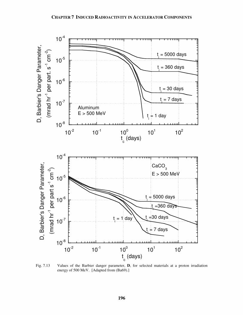
CHAPTER 7 INDUCED RADIOACTIVITY IN ACCELERATOR COMPONENTS
196
10-8
10-7
10-6
10-5
10-4
10-2 10-1 100 101 102
D, B
arbi
er's
Dan
ger P
aram
eter
,
(mra
d hr
-1 p
er p
art.
s-1 c
m-2
)
tc (days)
AluminumE > 500 MeV
ti = 5000 days
ti = 30 days
ti = 360 days
ti = 7 days
ti = 1 day
10-8
10-7
10-6
10-5
10-4
10-2 10-1 100 101 102
D, B
arbi
er's
Dan
ger P
aram
eter
,
(mra
d hr
-1 p
er p
art s
-1 c
m-2
)
tc (days)
ti = 5000 days
ti =360 days
ti =30 days
ti = 7 days
ti = 1 day
CaCO3
E > 500 MeV
Fig. 7.13 Values of the Barbier danger parameter, D, for selected materials at a proton irradiation
energy of 500 MeV. [Adapted from (Ba69).]
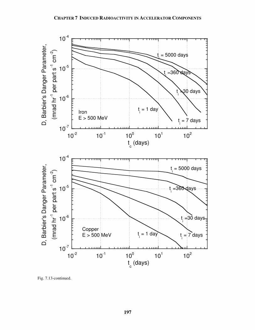
CHAPTER 7 INDUCED RADIOACTIVITY IN ACCELERATOR COMPONENTS
197
10-7
10-6
10-5
10-4
10-2 10-1 100 101 102
D, B
arbi
er's
Dan
ger P
aram
eter
,
(mra
d hr
-1 p
er p
art s
-1 c
m-2
)
tc (days)
ti = 5000 days
ti =360 days
ti =30 days
ti = 7 days
ti = 1 dayIron
E > 500 MeV
10-7
10-6
10-5
10-4
10-2 10-1 100 101 102
D, B
arbi
er's
Dan
ger P
aram
eter
,
(mra
d hr
-1 p
er p
art s
-1 c
m-2
)
tc (days)
ti = 5000 days
ti =360 days
ti =30 days
ti = 7 dayst
i = 1 day
CopperE > 500 MeV
Fig. 7.13-continued.
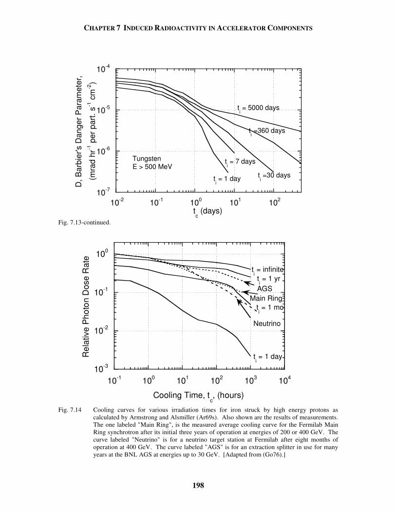
CHAPTER 7 INDUCED RADIOACTIVITY IN ACCELERATOR COMPONENTS
198
10-7
10-6
10-5
10-4
10-2 10-1 100 101 102
D, B
arbi
er's
Dan
ger P
aram
eter
,
(mra
d hr
-1 p
er p
art.
s-1 c
m-2
)
tc (days)
TungstenE > 500 MeV
ti = 5000 days
ti =360 days
ti =30 days
ti = 7 days
ti = 1 day
Fig. 7.13-continued.
10-3
10-2
10-1
100
10-1 100 101 102 103 104
Rel
ativ
e P
hoto
n D
ose
Rat
e
Cooling Time, tc, (hours)
ti = infiniteti = 1 yr
ti = 1 mo
ti = 1 day
AGSMain Ring
Neutrino
Fig. 7.14 Cooling curves for various irradiation times for iron struck by high energy protons as
calculated by Armstrong and Alsmiller (Ar69s). Also shown are the results of measurements. The one labeled "Main Ring", is the measured average cooling curve for the Fermilab Main Ring synchrotron after its initial three years of operation at energies of 200 or 400 GeV. The curve labeled "Neutrino" is for a neutrino target station at Fermilab after eight months of operation at 400 GeV. The curve labeled "AGS" is for an extraction splitter in use for many years at the BNL AGS at energies up to 30 GeV. [Adapted from (Go76).]
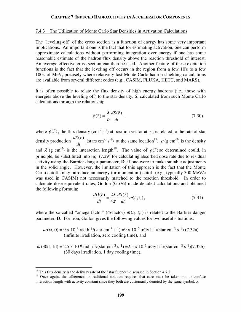
CHAPTER 7 INDUCED RADIOACTIVITY IN ACCELERATOR COMPONENTS
199
7.4.3 The Utilization of Monte Carlo Star Densities in Activation Calculations The "leveling-off" of the cross section as a function of energy has some very important implications. An important one is the fact that for estimating activation, one can perform approximate calculations without performing integration over energy if one has some reasonable estimate of the hadron flux density above the reaction threshold of interest. An average effective cross section can then be used. Another feature of these excitation functions is the fact that the leveling off occurs in the region from a few 10's to a few 100's of MeV, precisely where relatively fast Monte Carlo hadron shielding calculations are available from several different codes (e.g., CASIM, FLUKA, HETC, and MARS). It is often possible to relate the flux density of high energy hadrons (i.e., those with energies above the leveling off) to the star density, S, calculated from such Monte Carlo calculations through the relationship
( )
( )dS r
rdt
λφρ
=
, (7.30)
where φ( )
r , the flux density (cm-2 s-1) at position vector at r
, is related to the rate of star
density production dS r
dt( )
(stars cm-3 s-1) at the same location17. ρ (g cm-3) is the density
and λ (g cm-2) is the interaction length18. The value of ( )rφ so determined could, in principle, be substituted into Eq. (7.29) for calculating absorbed dose rate due to residual activity using the Barbier danger parameter, D, if one were to make suitable adjustments in the solid angle. However, the limitation of this approach is the fact that the Monte Carlo cutoffs may introduce an energy (or momentum) cutoff (e.g., typically 300 MeV/c was used in CASIM) not necessarily matched to the reaction threshold. In order to calculate dose equivalent rates, Gollon (Go76) made detailed calculations and obtained the following formula:
( ) ( )
( , )4 i c
dD r dS rt t
dt dtω
πΩ=
, (7.31)
where the so-called “omega factor” (ω-factor) ω (ti, tc ) is related to the Barbier danger parameter, D. For iron, Gollon gives the following values for two useful situations:
ω (∞, 0) = 9 x 10⁻⁶ rad h-1/(star cm-3 s-1) =9 x 10⁻² µGy h-1/(star cm-3 s-1) (7.32a) (infinite irradiation, zero cooling time), and ω (30d, 1d) = 2.5 x 10⁻⁶ rad h-1/(star cm-3 s-1) =2.5 x 10⁻² µGy h-1/(star cm-3 s-1)(7.32b) (30 days irradiation, 1 day cooling time).
17 This flux density is the delivery rate of the "star fluence" discussed in Section 4.7.2. 18 Once again, the adherence to traditional notation requires that care must be taken not to confuse interaction length with activity constant since they both are customarily denoted by the same symbol, λ.
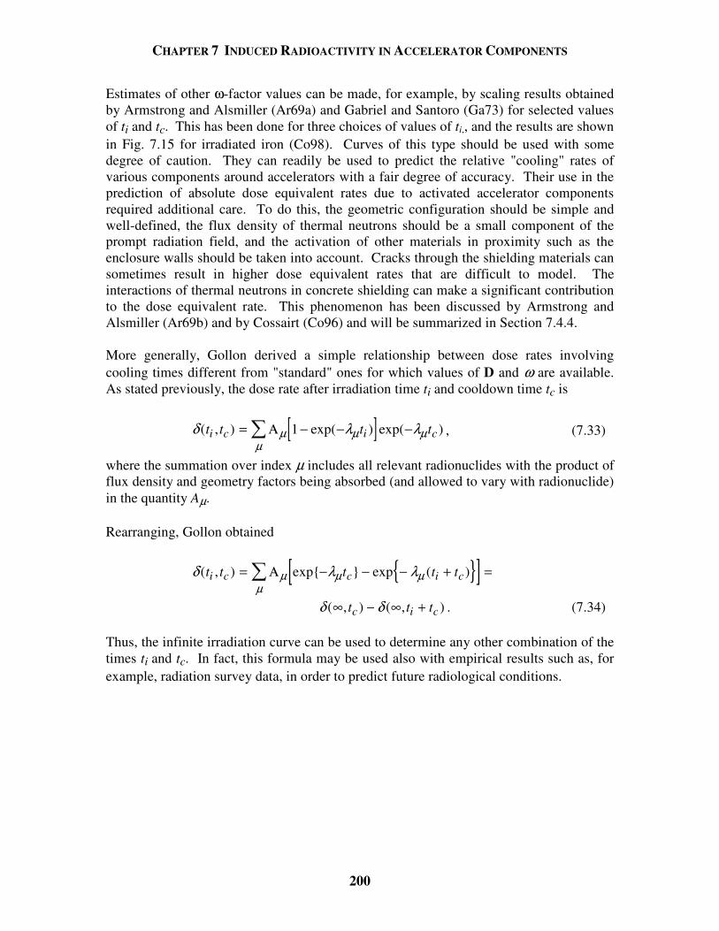
CHAPTER 7 INDUCED RADIOACTIVITY IN ACCELERATOR COMPONENTS
200
Estimates of other ω-factor values can be made, for example, by scaling results obtained by Armstrong and Alsmiller (Ar69a) and Gabriel and Santoro (Ga73) for selected values of ti and tc. This has been done for three choices of values of ti,, and the results are shown in Fig. 7.15 for irradiated iron (Co98). Curves of this type should be used with some degree of caution. They can readily be used to predict the relative "cooling" rates of various components around accelerators with a fair degree of accuracy. Their use in the prediction of absolute dose equivalent rates due to activated accelerator components required additional care. To do this, the geometric configuration should be simple and well-defined, the flux density of thermal neutrons should be a small component of the prompt radiation field, and the activation of other materials in proximity such as the enclosure walls should be taken into account. Cracks through the shielding materials can sometimes result in higher dose equivalent rates that are difficult to model. The interactions of thermal neutrons in concrete shielding can make a significant contribution to the dose equivalent rate. This phenomenon has been discussed by Armstrong and Alsmiller (Ar69b) and by Cossairt (Co96) and will be summarized in Section 7.4.4. More generally, Gollon derived a simple relationship between dose rates involving cooling times different from "standard" ones for which values of D and ω are available. As stated previously, the dose rate after irradiation time ti and cooldown time tc is
[ ]δ λ λµµ
µ µ( , ) exp( ) exp( )t t t ti c i c= − − −Α 1 , (7.33)
where the summation over index µ includes all relevant radionuclides with the product of flux density and geometry factors being absorbed (and allowed to vary with radionuclide) in the quantity Aµ. Rearranging, Gollon obtained
[ ]δ λ λµµ
µ µ( , ) exp exp ( )t t t t ti c c i c= − − − + =Α
δ δ( , ) ( , )∞ − ∞ +t t tc i c . (7.34) Thus, the infinite irradiation curve can be used to determine any other combination of the times ti and tc. In fact, this formula may be used also with empirical results such as, for example, radiation survey data, in order to predict future radiological conditions.
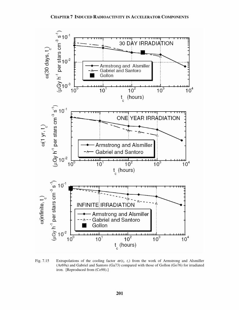
CHAPTER 7 INDUCED RADIOACTIVITY IN ACCELERATOR COMPONENTS
201
Fig. 7.15 Extrapolations of the cooling factor ω (ti, tc) from the work of Armstrong and Alsmiller
(Ar69a) and Gabriel and Santoro (Ga73) compared with those of Gollon (Go76) for irradiated iron. [Reproduced from (Co98).]
CHAPTER 7 INDUCED RADIOACTIVITY IN ACCELERATOR COMPONENTS
202
A reliable method for connecting the production of "stars" in material (e.g., as calculated by a Monte Carlo code) to the production of atoms of some radionuclide is by the ratios of cross sections. Thus, at some point in space, r
, the rate of production of atoms per
cm3, ( )in r
, of some radionuclide, i, is approximately given by
( ) ( ) ( )i i i
in in
dn r dS r dS rdt dt dt
σσ
Σ≈ =Σ
, (7.35)
where one essentially scales the star density production rate (e.g., stars cm-3 s-1) by the ratio of the production (reaction) cross section for the nuclide of interest, σi, to the total inelastic cross section σin or, equivalently, by the ratio of the macroscopic cross sections, (Σi/Σin). The phenomena will obey the usual activation equation. The reason this is approximate is due to the standard concerns about constancy of cross sections with energy, the lack of perfect "matching" of effective reaction thresholds, etc. 7.4.4 Uniform Irradiation of the Walls of an Accelerator Enclosure Somewhat special considerations may apply to the concrete shielding surrounding accelerators. As was seen before in Table 6.2, ordinary concrete typically contains a partial density of about 0.04 g cm-3 of sodium. This "typical" value varies a great deal due to the variety of minerals that might be present in local concrete. The significance of this seemingly small additive is that the naturally dominant isotope present is 23Na. This nucleus has the relatively large thermal neutron capture cross section of 535 mb. Patterson (Pa58) determined that average thermal neutron flux density, φth, in a concrete room is approximately given as follows:
φthQ
S=
125. (cm-2s-1), (7.36)
where Q is the number of fast neutrons produced per second in the enclosure and S is the inside surface area of the enclosure (cm2). Thus, a substantial flux density of thermal neutrons can be present in an accelerator room and this flux can produce significant amount of 24Na with its 15-hour half-life. The pair of relatively high energy photons emitted in its decay (1.37 and 2.75 MeV) further enhances the residual radioactivity hazard. Furthermore, while the dose due to activated components falls off radially with distance, if absorption by the air is not significant the photon flux density due to activation of the walls of an empty room uniformly irradiated by such thermal neutrons is a constant. Thus, the absorbed dose rate due to the walls anywhere inside the enclosure will be equal to the absorbed dose rate at the wall. This has been explicitly demonstrated for cylinders by Armstrong and Barish (Ar69b) and is also true for the interior of all mathematically “well-behaved” closed surfaces (Co96). This fact can readily be demonstrated by analogy to the Gauss Law in electrostatics19 as follows by examining the situation in Fig. 7.16. 19 The Gauss law of electrostatics has been treated in detail by others; e.g., Jackson (Ja75) and Konopinski (Ko81).
CHAPTER 7 INDUCED RADIOACTIVITY IN ACCELERATOR COMPONENTS
203
Z
YX
• P
dA
r′ – rr′
r
n
O
Fig. 7.16 Geometry for deriving the relationship between a surface of uniform emission and the flux density at any point within it. [Reproduced from (Co96).]
Consider a simple, closed surface that emits an omnidirectional flux density of some particle φo (e.g., particles cm-2s-1) that is constant over the surface. One wants to calculate the flux density at some arbitrary point in space P within the surface. P is located at radius vector r
. Consider further the contributions of the particles emitted by
some elemental area dA
at P where dA
is perpendicular to the surface at coordinate vector r
. The solid angle subtended at P by dA
is
2
ˆdA nd
r r
•Ω =′ −
, (7.37)
where the unit vector n is given by
rrrr
n
−′−′
=ˆ . (7.38)
But the increment of flux at point P due to elemental area dA
is given by
2
ˆ4 rr
nAdd
−′•=
πφφ ο .
Thus,
4
od dφφπ
= Ω and 4 4
ood
π
φ φπ
Ω = . (7.39)
CHAPTER 7 INDUCED RADIOACTIVITY IN ACCELERATOR COMPONENTS
204
In some situations it is important to minimize the amount of sodium in the concrete ingredients in order to reduce exposures to individuals conducting maintenance on the accelerator. In fact, the phenomena described above has been noticed at accelerators and sometimes leads to "disappointment" in how little gamma-ray exposure rates are reduced when activated accelerator components are removed from enclosures with equally activated walls. For example, Armstrong and Barish (Ar69b) have calculated residual dose rates inside a cylindrical accelerator tunnel due to both the magnets and the concrete walls for 3 GeV protons incident on iron. These authors also included some other reactions due to higher energy neutrons, such as spallation, that are capable of also producing 24Na from common ingredients of concrete. The results are shown in Fig. 7.17 for the surface at the tunnel wall. The discussion of the production of radioactivity continues in Chapter 8 with specific emphasis on environmental radiation protection.
10-2
10-1
100
10-1 100 101 102 103
Rel
ativ
e P
hoto
n D
ose
Rat
e
cooling time, tc (hours)
From other radionuclidesin concrete
From 24Na in concrete
From ironTotal
Fig. 7.17 Photon dose rate at surface of tunnel wall after infinite irradiation time for concrete containing
one per cent sodium by weight. [Adapted from (Ar69b).]
CHAPTER 7 INDUCED RADIOACTIVITY IN ACCELERATOR COMPONENTS
205
Problems 1. A 1 mA beam of 30 MeV electrons is absorbed by an aluminum target. Calculate
the saturation activities of all major radionuclides produced in the target. Assuming no self-absorption and an infinitely long irradiation period, what will the absorbed dose rate at a distance of 2 meters away immediately after beam shutdown and one hour later? The target can be assumed to be a point source for this estimate.
2. A copper beam stop has been bombarded with high energy hadrons for 30 days
and exhibits a dose rate of 100 mrem hr-1 at 1 meter away 1 day after the beam is turned off. Maintenance work needs to be scheduled in the vicinity within the next 6 months. Using both Gollon's Rule No. 3 and the Barbier Danger parameter curves, predict the cooling curve and determine when the dose rate is less than a 20 mrem hr-1 maintenance work criteria. Make a table of dose rate versus cooling time in days for both methods. How well do the two methods agree? (Hint: Use the initial value of the dose rate to scale values of D.)
3. A 100 GeV beam (1012 protons s-1) strikes the center of a large solid iron cylinder
30 cm in radius for 30 days. Use the star density curves from the Appendix C and the "ω" factors calculated by Gollon to estimate the residual dose rate after 1 day cooldown at contact with the side of the cylinder in the "hottest" spot. Using Gollon's third rule, how long must the repair crew wait to service this item in a contact radiation field of absorbed dose rate < 10 rad hr-1?
4. A copper target is bombarded with high energy protons such that 10 stars per incident proton are produced. If the incident beam is 1011 protons s-1, what is the specific activity (average) of 54Mn that is produced after two years of operation? 54Mn has a high energy spallation production cross section of about 20 mb in Cu. The target is a cylinder, 10 cm radius by 15 cm long. The half-life of 54Mn is 312 days. Express the answer in both Bq cm-3 and Ci cm-3. (Hint: This problem is best if the calculation is done at saturation and then corrected for the non-infinite irradiation time. Also, one needs to use the inelastic cross section given, for example, in Chapter 4.)
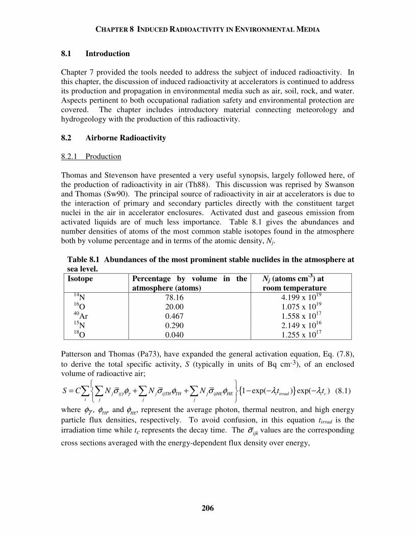
CHAPTER 8 INDUCED RADIOACTIVITY IN ENVIRONMENTAL MEDIA
206
8.1 Introduction Chapter 7 provided the tools needed to address the subject of induced radioactivity. In this chapter, the discussion of induced radioactivity at accelerators is continued to address its production and propagation in environmental media such as air, soil, rock, and water. Aspects pertinent to both occupational radiation safety and environmental protection are covered. The chapter includes introductory material connecting meteorology and hydrogeology with the production of this radioactivity. 8.2 Airborne Radioactivity 8.2.1 Production Thomas and Stevenson have presented a very useful synopsis, largely followed here, of the production of radioactivity in air (Th88). This discussion was reprised by Swanson and Thomas (Sw90). The principal source of radioactivity in air at accelerators is due to the interaction of primary and secondary particles directly with the constituent target nuclei in the air in accelerator enclosures. Activated dust and gaseous emission from activated liquids are of much less importance. Table 8.1 gives the abundances and number densities of atoms of the most common stable isotopes found in the atmosphere both by volume percentage and in terms of the atomic density, Nj.
Table 8.1 Abundances of the most prominent stable nuclides in the atmosphere at sea level. Isotope Percentage by volume in the
atmosphere (atoms) Nj (atoms cm-3) at room temperature
14N 78.16 4.199 x 10¹⁹ 16O 20.00 1.075 x 10¹⁹ 40Ar 0.467 1.558 x 10¹⁷ 15N 0.290 2.149 x 10¹⁶ 18O 0.040 1.255 x 10¹⁷
Patterson and Thomas (Pa73), have expanded the general activation equation, Eq. (7.8), to derive the total specific activity, S (typically in units of Bq cm-3), of an enclosed volume of radioactive air;
1 exp( ) exp( )j ij j ijTH TH j ijHE HE i irrad i ci j j j
S C N N N t tγ γσ φ σ φ σ φ λ λ
= + + − − −
(8.1)
where φγ , φTH, and φHE, represent the average photon, thermal neutron, and high energy particle flux densities, respectively. To avoid confusion, in this equation tirrad is the irradiation time while tc represents the decay time. The ijkσ values are the corresponding
cross sections averaged with the energy-dependent flux density over energy,
CHAPTER 8 INDUCED RADIOACTIVITY IN ENVIRONMENTAL MEDIA
207
max
min
max
min
( ) ( )
( )
ijk k
k
E
Eijk E
E
dE E E
dE E
σ φσ
φ=
, (8.2)
where the limits of integration correspond to the three broad phenomenological ranges in the summation. The constant C is the conversion to specific activity and is equal to unity for activity in Becquerels cm-3 if all the units of length implicit in the quantities in Eq. (8.1) are expressed in cm. The outer sum over index i includes all possible radionuclides produced and the sum over the index j is over the parent atoms found in air. The flux densities are, without further information, the average over some relevant spatial volume. Table 8.2 lists the radionuclides that can be produced from the principle constituents in air along with the reaction mechanisms associated with their production and an estimate of the average production cross section. The large cross sections for (n, γ) and (n, p) reactions are for captures of neutrons of thermal energies (<En> ≈ 0.025 eV) while the remaining cross sections are generally the saturation cross sections found in the region above approximately a few 10’s of MeV. The γ-induced reactions are present at virtually all accelerators and at most energies. The corresponding cross sections will, of course, be energy-dependent especially at energies just above the reaction thresholds. 8.2.2 Accounting for Ventilation Adjustments for the presence of ventilation can be quite conveniently made for a given radionuclide by using an effective decay constant, λ ′ , that includes the physical decay constant, λ, along with a ventilation term, r; r+=′ λλ , (8.3)
where VD
r = ,
with D being the ventilation rate in air volume per unit time and V being the enclosure volume. Thus r is the number of air changes per unit time. The applicable differential equation, an extension of Eq. (7.4) with ventilation included, is
( ) ( ) ( )dn
n t rn t N n t Ndt
λ σφ λ σφ′ ′ ′ ′ ′= − − + = − + . (8.4)
After an irradiation time, ti, with no initial activation, the solution by analogy with Eq. (7.5) is
[ ] ( ) 1 exp ( )i i
Nn t r t
rσφ λ
λ′ = − − +
+. (8.5)
So the specific activity with mixing, ( )ia t′ , is given by
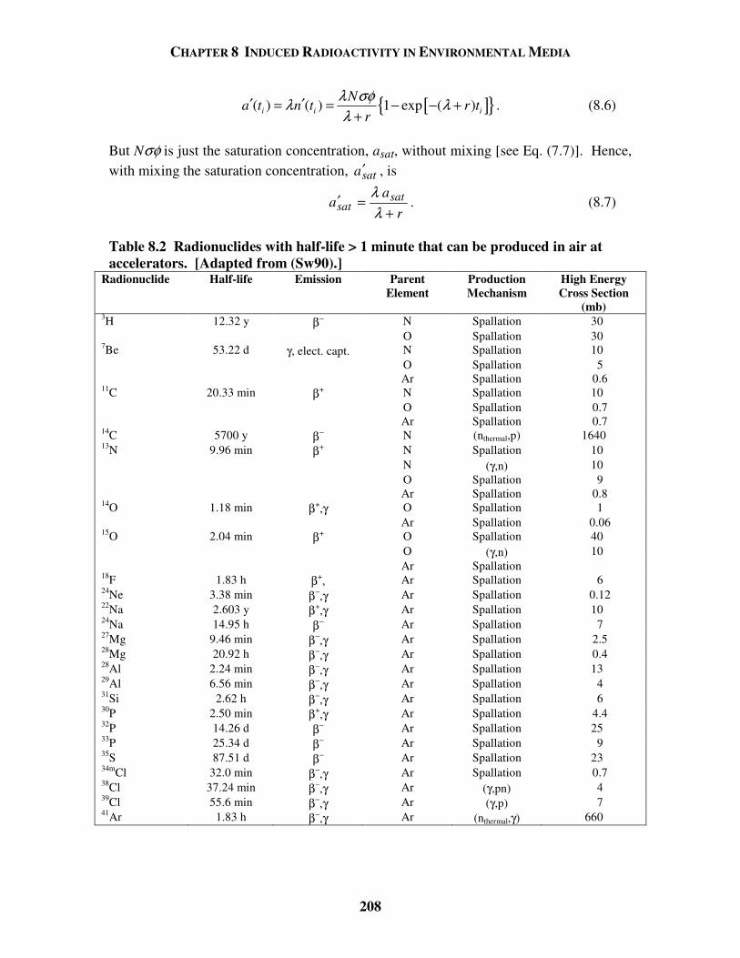
CHAPTER 8 INDUCED RADIOACTIVITY IN ENVIRONMENTAL MEDIA
208
[ ] ( ) ( ) 1 exp ( )i i i
Na t n t r t
rλ σφλ λλ
′ ′= = − − ++
. (8.6)
But Nσφ is just the saturation concentration, asat, without mixing [see Eq. (7.7)]. Hence, with mixing the saturation concentration, sata′ , is
r
aa sat
sat +=′
λλ
. (8.7)
Table 8.2 Radionuclides with half-life > 1 minute that can be produced in air at accelerators. [Adapted from (Sw90).]
Radionuclide Half-life Emission Parent Element
Production Mechanism
High Energy Cross Section
(mb) 3H 12.32 y β− N Spallation 30 O Spallation 30 7Be 53.22 d γ, elect. capt. N Spallation 10 O Spallation 5 Ar Spallation 0.6 11C 20.33 min β+ N Spallation 10 O Spallation 0.7 Ar Spallation 0.7 14C 5700 y β− N (nthermal,p) 1640
13N 9.96 min β+ N Spallation 10 N (γ,n) 10 O Spallation 9 Ar Spallation 0.8 14O 1.18 min β+,γ O Spallation 1 Ar Spallation 0.06 15O 2.04 min β+ O Spallation 40 O (γ,n) 10 Ar Spallation 18F 1.83 h β+, Ar Spallation 6 24Ne 3.38 min β−,γ Ar Spallation 0.12 22Na 2.603 y β+,γ Ar Spallation 10 24Na 14.95 h β− Ar Spallation 7 27Mg 9.46 min β−,γ Ar Spallation 2.5 28Mg 20.92 h β−,γ Ar Spallation 0.4 28Al 2.24 min β−,γ Ar Spallation 13 29Al 6.56 min β−,γ Ar Spallation 4 31Si 2.62 h β−,γ Ar Spallation 6 30P 2.50 min β+,γ Ar Spallation 4.4 32P 14.26 d β− Ar Spallation 25 33P 25.34 d β− Ar Spallation 9 35S 87.51 d β− Ar Spallation 23 34mCl 32.0 min β−,γ Ar Spallation 0.7 38Cl 37.24 min β−,γ Ar (γ,pn) 4 39Cl 55.6 min β−,γ Ar (γ,p) 7 41Ar 1.83 h β−,γ Ar (nthermal,γ) 660
CHAPTER 8 INDUCED RADIOACTIVITY IN ENVIRONMENTAL MEDIA
209
Since low energy accelerators must, for other reasons, contain their beams in continuous vacuum systems, the activation of air at these machines is greatly minimized. At high energy accelerators, it is quite common to have air gaps at certain interface points to accommodate devices associated with beam targetry or beamline diagnostic instrumentation which render continuous vacuum impractical. These "air gaps" are only found in external beam lines and possibly in linear accelerators. The beam in a circular accelerator or storage ring is, of necessity, contained in continuous vacuum since any air gaps, if traversed multiple times by the beam particles, would result in an unacceptable rate of beam loss. In addition, the large multiplicity of secondary particles produced as a part of cascade processes, either electromagnetic or hadronic, can produce airborne radioactivity external to the beamline vacuum. If the accelerator enclosures were completely sealed, there would be no releases to the outside world and the hazard of these airborne radionuclides would be entirely restricted to those who might have to enter the enclosures. This would, however, allow the longer-lived radionuclides to build up in accord with Eq. (8.1). Also, ventilation is generally needed to provide cooling of components and fresh breathing air for workers. Typically, the average residence time of air in accelerator enclosures is limited to a range of between approximately 30 minutes and not much longer than one hour20. Thus, the airborne radionuclides in the accelerator environment, in equilibrium, will have half-lives only up to the order of one hour. The residence time of the air in conjunction with the cross sections determines the radionuclides of importance. 8.2.3 Propagation of Airborne Radionuclides in the Environment The other consideration concerning airborne radioactivity is that associated with the dose delivered to members of the general public when radionuclides are released to the atmosphere external to the accelerator enclosure. The U. S. Environmental Protection Agency (EPA) has placed an annual limit of 10 mrem on dose equivalent to members of the general public due to the operations of DOE facilities, comparable to limits applied to other facilities, and has also placed stringent regulations on how such releases are to be measured (CFR89). An annual dose equivalent of such small value is usually difficult or impossible to measure at distant locations. Thus, the standard practice is to measure the activity released and then use calculational models to estimate the maximum dose equivalent that actual members of the public could receive. The regulations prescribe the specific computer codes that must be used to perform these calculations through the use of a Gaussian plume model that combines input data on the release of radioactivity with meteorological information. The details of such computer modeling will not be described here. Examples of such plume models are given in textbooks and the results depend on details of the meteorological conditions. A short synopsis is given here.
20 However, at some facilities releases of airborne radionuclides to the outdoors are minimized by greatly restricting the release rate of air during accelerator operations. When personnel accesses are made subsequent to operations, the ventilation rate must then be increased to levels consistent with good industrial hygiene practice. The principles described in this chapter can be used to evaluate the magnitude and radionuclide composition of the air released under these more complex operational conditions.
CHAPTER 8 INDUCED RADIOACTIVITY IN ENVIRONMENTAL MEDIA
210
8.2.3.1 Propagation of Airborne Radioactivity - Tall Stacks Concentrations of radionuclides at distant locations can be estimated analytically using the so-called Sutton's equation to be described shortly. Due to the nature of accelerator operations, only "steady-state" conditions are considered since transient accidental releases from accelerators are unlikely. A good description that applies to rather tall ( > 25 m) release points has been presented by Cember (Ce69). Such release points are commonly called stacks. More details have been provided by Slade (Sl68). The dispersion is mainly characterized by dilution of the radionuclides and their eventual return to ground level breathing zones. The meteorological conditions of major importance to this topic are illustrated in Fig. 8.1. Relevant stability classes have been developed that describe the various possibilities. Descriptions of these stability classes are given in Table 8.3.
Fig. 8.1 Effect of atmospheric temperature gradient or lapse rate on a displaced volume of air for
various conditions: a) Unstable lapse rate; b) Stable lapse rate; c) Neutral lapse rate [Reproduced from (Sl68).]
CHAPTER 8 INDUCED RADIOACTIVITY IN ENVIRONMENTAL MEDIA
211
Table 8.3 Atmospheric stability classes for use with Sutton's equation. [Adapted from (Sl68).] stable: No heat is gained or lost by a parcel of air that rises and expands adiabatically with
falling temperature. The adiabatic cooling with rise normally corresponds to a gradient of about 5.4 oF/1000 ft (1 oC/100 meters) for dry air and about 3.5 oF/1000 ft (0.6 oC/100 meters) for moist air. If the atmospheric temperature gradient is less than adiabatic, but still negative, stability is achieved because a rising parcel cools faster than its surroundings and then tends to sink. A sinking parcel is warmer than its surroundings and thus is less dense and tends to rise. This restricts the width of the plume and consequently decreases dilution.
inversion: If the temperature gradient is such that the temperature increases with height, then an
inversion occurs. Rising effluent from a "stack" becomes much denser than its surroundings and thus sinks. The effluent is thus more limited in its ascent and this, too, serves to limit dilution.
superadiabatic: If the rate of decrease of temperature with elevation is greater than that in adiabatic
conditions, an unstable condition results which promotes the vertical dispersion, and hence dilution. A rising parcel does not cool fast enough due to its expansion and therefore remains warmer and continues to rise. Likewise, a falling parcel continues to fall.
Sutton's equation, as adapted here by Cember (Ce69), for determining the concentration of a short-lived radionuclide released by a tall stack, is
c x yQ
C ux ux y
h y
C xn n( , ) exp exp= − +
−+
− −
22 2
2 22 2
2 2πλ
, (8.8)
where the exponential involving the decay constant λ conservatively allows for radioactive decay in transit for a particular radionuclide. The rest of the quantities are as follows:
(x,y,z) are Cartesian coordinates to the point of measurement from the foot of the stack (meters) where x is along the centerline of the plume as determined by the wind direction (downwind), y is the transverse coordinate, and z is the vertical coordinate; c x y( , ) is the average concentration (activity m-3) at ground level (z = 0); Q is the emission rate of (activity s-1); u is the mean wind speed (meters s-1); C is the virtual diffusion constant in lateral and vertical directions (Table 8.4); n is a dimensionless parameter related to the atmospheric conditions (Table 8.4); and h is the effective chimney height (if the gas has significant emission velocity) determined from the actual chimney height ha by
h h dvu
TTa= +
+
1 41
. ∆. (8.9)
CHAPTER 8 INDUCED RADIOACTIVITY IN ENVIRONMENTAL MEDIA
212
In Eq. (8.9) d is the outlet diameter (meters), v is the exit velocity of the gas (meters s-1), and ∆T/T is the difference between the temperature of the gas and the ambient outdoor temperature divided by the absolute temperature of the gas, T. Table 8.4 gives values for certain parameters to be used in Eq. (8.8). Table 8.4 Diffusion (C2) and Stability (n) parameters for Cember's version of Sutton's Equation, Eq. (8.8). [Adapted from (Ce69).] Lapse Rate C2
Effective Chimney Height, h, (meters) n 25 50 75 100 Superadiabatic 0.20 0.043 0.030 0.024 0.015 Stable 0.25 0.014 0.010 0.008 0.005 Moderate Inversion 0.33 0.006 0.004 0.003 0.002 Large Inversion 0.5 0.004 0.003 0.002 0.001 8.2.3.2 Propagation of Airborne Radioactivity - Short Stacks The above representation of Sutton's equation is a useful one where tall stacks are involved. However, at typical accelerator facilities it is uncommon for stacks to be very tall. Again for purposes of this discussion, only steady state conditions continuous in time are treated here. For such calculations, the concentration as a function of coordinates, c (x,y,z), defined as for the tall stacks, is given by a somewhat different formulation of Sutton's equation which uses the same coordinate system (Sl68);
+−+
−−
−
+−=2
2
2
2
2
222
2)(
exp2
)(exp
2expexp
2),,(
zzyzy
hzhzyyx
uuQ
zyxcσσσ
λσπσ
.
(8.10) For the common situation of interest where the receptor location of concern is at ground level (z = 0), this simplifies to
2 2
2 22 2( , , 0) exp exp
2 2y z y z
Q y hc x y x y
u uλ
πσ σ σ σ
= − + − + , (8.11)
where the presence of the ground as a "barrier" to the flux is taken into account. In these equations, the quantity h is effective stack height above the ground in meters and σy(x) and σz(x), implicit functions of downwind coordinate x, are dispersion coefficients that have units of length (meters). All other quantities are the same as given above for tall stacks. These variables are, of course, determined from the meteorological conditions. In Eq. (8.10) and Eq. (8.11), the exponential involving the decay constant λ again conservatively allows for radioactive decay in transit for a particular radionuclide.
CHAPTER 8 INDUCED RADIOACTIVITY IN ENVIRONMENTAL MEDIA
213
Table 8.5 gives an alternative scheme for classifying the meteorological conditions. The classification may then be used with the curves in Figs. 8.2 and 8.3 to determine the values of σy and σz as a function of the coordinate x for use in Eqs. (8.10) and (8.11). Table 8.5 Relation of turbulence types to weather conditions. [Adapted from (Sl68).] A-Extremely unstable conditions D-neutral conditionsa B-Moderately unstable conditions E-Slightly stable conditions C-Slightly unstable conditions F-Moderately stable conditions Surface Wind
Speed Daytime insolation Nightime conditions
(m/sec) Strong Moderate Slight Thin overcast or > 4/8
cloudinessb
< 3/8 cloudiness
<2 A A-B B 2 A-B B C E F 4 B B-C C D E 6 C C-D D D D
>6 C D D D D aApplicable to heavy overcast, day or night bThe degree of cloudiness is defined as that fraction of the sky above the local apparent horizon which is covered by clouds. Airborne radioactivity releases can be minimized by limiting the ventilation rates during operations when people are not present in the
enclosure (see footnote, this chapter), delaying the actual emissions by requiring long pathways to the ventilation "stacks",
and minimizing air gaps in the beam. 8.2.4 Radiation Protection Standards for Airborne Radioactivity The airborne radioactivity is of primary concern to workers who might enter the enclosure to perform maintenance activities and thus are classified as "occupational workers". Since the principal radionuclides are of relative short half-life, the hazard is largely due to the "immersion" in a “cloud” of external dose rather than a gaseous ingestion hazard such as might be found in operations involving the processing of long-lived radioactive materials. The latter leads to long-term internal radiation exposures. Regulatory authorities, guided by recommendations of the International Commission on
CHAPTER 8 INDUCED RADIOACTIVITY IN ENVIRONMENTAL MEDIA
214
100
101
102
103
104
102 103 104 105
ABCDEF
σ y, Hor
izon
tal D
ispe
rson
Coe
ffici
ent (
met
ers)
Distance From Source (meters)
Fig. 8.2 Horizontal diffusion constants, σy , as a function of downwind distance, x, from the source for turbulence types defined in Table 8.5. [Adapted from (Sl68).]
CHAPTER 8 INDUCED RADIOACTIVITY IN ENVIRONMENTAL MEDIA
215
100
101
102
103
102 103 104 105
ABCDEFσ z, V
ertic
al D
ispe
rsio
n C
oeffi
cien
t (m
eter
s)
Distance from Source (meters)
Fig. 8.3 Vertical diffusion constants, σz , as a function of downwind distance, x, from the source for turbulence types defined in Table 8.5. [Adapted from (Sl68).]
CHAPTER 8 INDUCED RADIOACTIVITY IN ENVIRONMENTAL MEDIA
216
Radiation Protection (ICRP) and National Council on Radiation Protection and Measurements (NCRP), have established Derived Air Concentrations (DACs) for radiation workers. These regulatory standards have supplanted the Maximum Permissible Concentrations (MPCs) formerly employed for this purpose that reflected methodologies that have subsequently been updated by the ICRP. DACs, as were MPCs, are based upon the receipt of 5000 mrem of dose equivalent if the entire working year (≈ 2000 hours, or 40 hours weekly) is spent working in a concentration corresponding to "1 DAC". A concentration as large as one DAC is rarely encountered in accelerator radiation environments. Similarly, for members of the general public, values of Derived Concentration Guides (DCGs) have been tabulated that would result in the receipt of 100 mrem of dose equivalent by an individual who spent all of the time in one year breathing such air. Table 8.6 gives representative values of these circumstance-dependent maximum concentrations, Cmax, for accelerator-produced radionuclides in air based upon present U. S. Department of Energy Orders (DOE90) and Regulations (CFR93) along with companion values determined for accelerator-produced radionuclides not included in the cited references that have been calculated by Höfert (Hö69). For some radionuclides commonly found at accelerators, DOE regulations (CFR93) gives two values of DAC, one for air inhaled into the lungs and the other for immersion in an infinite cloud of γ-emitting radionuclides. Table 8.6 DACs and DCGs (Air) for radiation workers and the general population. These represent maximum concentrations for radionuclide i, Cmax,i, depending upon the circumstances of exposure (see text).21
DAC- U. S. DOE Radiation Worker
DCG-General Populationd
Immersion Exposure [50 mSv y-1 (40 h week-1)]
Inhaled Air Exposureb [50 mSv y-1
(40 h week-1)] Infinite Radius Cloudb 4 m Radius Cloudc
[1 mSv year-1
(168 h week-1)]
(µµµµCi m-3) (Bq m-3) (µµµµCi m-3) (Bq m-3) (µµµµCi m-3) (Bq m-3) (µµµµCi m-3) (Bq m-3) 3H 20 8 x 10⁵ unlisted unlisted unlisted unlisted 0.1 3.7 x 10³
7Be 8 3 x 10⁵ unlisted unlisted unlisted unlisted 0.04 1.5 x 10³
11C 200 6 x 10⁶ 4 1 x 10⁵ 59 2.2 x 10⁶ 0.02 7.4 x 10²
13N unlisted unlisted 4 1 x 10⁵ 41 1.5 x 10⁶ 0.02 7.4 x 10² 15O unlisted unlisted 4 1 x 10⁵ 27 1.0 x 10⁶ 0.02 7.4 x 10² 22Na 0.3 1 x 10⁴ unlisted unlisted unlisted unlisted 0.001 37 24Na 2 8 x 10⁴ 0.9 3 x 10⁴ unlisted unlisted 0.004 1.5 x 10²
41Ar unlisted unlisted 3 1 x 10⁵ 47 1.8 x 10⁶ 0.01 3.7 x 10²
Immersion conditions are more likely to be the dominant exposure mechanism due to activated air at accelerators. However, for occupational exposures, the sizes of the "clouds" are not likely to be "infinite" but will be determined by the dimensions of the 21 The values in Table 8.6 are, essentially, “worst case” values from the references cited. The user must take care to apply the specific values promulgated by the regulatory authority having jurisdiction. Furthermore, given the primacy of “customary” rather than SI units in United States Regulations, the former is generally taken to be limiting quantity. Also, conversion between the two sets of units in regulatory tables is generally only performed to one significant figure, as reflected here. Where choices needed to be made between day, week, or year exposures, the most restrictive value was taken.
CHAPTER 8 INDUCED RADIOACTIVITY IN ENVIRONMENTAL MEDIA
217
accelerator enclosures. While Höfert's calculations are connected with the obsolete MPCs values, they remain of importance because they recognized that "immersion dose" is highly sensitive to the size of the cloud and that clouds of infinite extent are rare inside buildings at accelerators. Höfert calculated the equivalent of DACs for clouds of various sizes. Table 8.6 gives those for clouds of 4 meters radius that might be typical of an accelerator enclosure. For the general population, Höfert postulated an infinite cloud, since such exposure would presumably occur outdoors. Mixtures of radionuclides are commonly encountered. To account for the presence of multiple radionuclides, the set of individual radionuclide concentrations in the air, Ci, must satisfy the following inequality:
CC
i
ii max, ≤ 1, (8.12)
where Cmax,i is the regulatory standard for the ith radionuclide, dependent upon the circumstances of the exposure. 8.2.5 Production of Airborne Radionuclides at Electron Accelerators At electron accelerators, significant air activation will not occur without bremsstrahlung because the nuclear cross sections of electrons are about two orders of magnitude smaller than those of photons (Sw79a)22. This airborne radioactivity is generally short-lived and the concentrations, as shall be seen in what follows, are usually quickly reduced to levels where the exposure rates (R h-1), or equivalently the absorbed dose rates (rads h-1) are small compared to those due to the accelerator components. This result is because the radiation length of air is so much longer than that of any solid material (see Table 1.2). Swanson (Sw79a) has calculated the saturation activities produced in air normalized to the electron beam power with the results provided in Table 8.7. The results of these calculations are normalized to unit path length and to beam power. To use them to determine the volume specific activity (e.g., Ci cm-3) in a given accelerator enclosure, one must multiply the tabulated values by the available bremsstrahlung path length23 and divide by the enclosure volume. The results found in this table were calculated in a manner completely analogous to those given in Table 7.2 for other materials. For energies close to the threshold of an individual reaction, the rise of activity with beam energy, Eo, (see Section 7.3.2 and Fig. 3.7) must be considered. 41Ar is produced in the thermal neutron capture (n, γ) reaction most copiously where there are high fluences of moderated neutrons present, typically near water-cooled targets and in concrete enclosures. 3H, 14C, and 7Be are too long-lived to be at levels anywhere near saturation and usually do not merit further consideration.
22 The reverse is true for toxic gas production, which occurs by a chemical, rather than nuclear, transformation and whose reaction rate is closely proportional to the integral absorbed dose to the air. Such dose is generally higher if the primary electron beam does not strike a target to produce bremsstrahlung but rather is directly delivered to air. The production of such toxic gases, most notably ozone (O3) is beyond the scope of this text but has been covered adequately by Swanson (Sw79a). 23 The available path length would either be set by the physical dimensions of the room or, for a large room, by the attenuation length of the bremsstrahlung radiation in air.
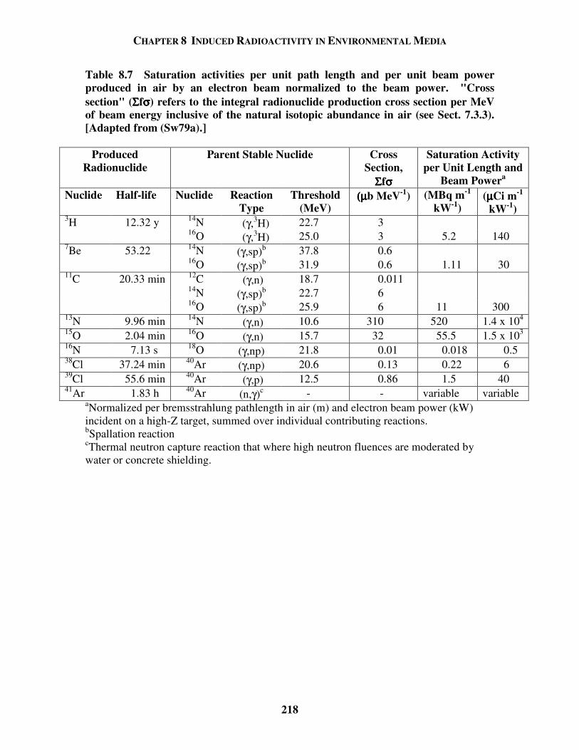
CHAPTER 8 INDUCED RADIOACTIVITY IN ENVIRONMENTAL MEDIA
218
Table 8.7 Saturation activities per unit path length and per unit beam power produced in air by an electron beam normalized to the beam power. "Cross section" (ΣΣΣΣfσσσσ) refers to the integral radionuclide production cross section per MeV of beam energy inclusive of the natural isotopic abundance in air (see Sect. 7.3.3). [Adapted from (Sw79a).]
Produced Radionuclide
Parent Stable Nuclide Cross Section,
ΣΣΣΣfσσσσ
Saturation Activity per Unit Length and
Beam Powera
Nuclide Half-life Nuclide Reaction Type
Threshold (MeV)
(µ(µ(µ(µb MeV-1) (MBq m-1 kW-1)
(µµµµCi m-1 kW-1)
3H 12.32 y 14N (γ,3H) 22.7 3
16O (γ,3H) 25.0 3 5.2 140
7Be 53.22 14N (γ,sp)b 37.8 0.6 16O (γ,sp)b 31.9 0.6 1.11 30 11C 20.33 min 12C (γ,n) 18.7 0.011 14N (γ,sp)b 22.7 6
16O (γ,sp)b 25.9 6 11 300
13N 9.96 min 14N (γ,n) 10.6 310 520 1.4 x 10⁴
15O 2.04 min 16O (γ,n) 15.7 32 55.5 1.5 x 10³
16N 7.13 s 18O (γ,np) 21.8 0.01 0.018 0.5 38Cl 37.24 min 40Ar (γ,np) 20.6 0.13 0.22 6 39Cl 55.6 min 40Ar (γ,p) 12.5 0.86 1.5 40 41Ar 1.83 h 40Ar (n,γ)c - - variable variable
aNormalized per bremsstrahlung pathlength in air (m) and electron beam power (kW) incident on a high-Z target, summed over individual contributing reactions. bSpallation reaction cThermal neutron capture reaction that where high neutron fluences are moderated by water or concrete shielding.
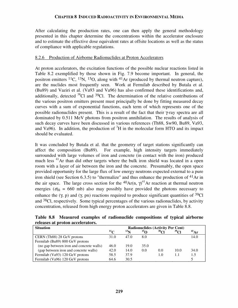
CHAPTER 8 INDUCED RADIOACTIVITY IN ENVIRONMENTAL MEDIA
219
After calculating the production rates, one can then apply the general methodology presented in this chapter determine the concentrations within the accelerator enclosure and to estimate the effective dose equivalent rates at offsite locations as well as the status of compliance with applicable regulations. 8.2.6 Production of Airborne Radionuclides at Proton Accelerators At proton accelerators, the excitation functions of the possible nuclear reactions listed in Table 8.2 exemplified by those shown in Fig. 7.9 become important. In general, the positron emitters 11C, 13N, 15O, along with 41Ar (produced by thermal neutron capture), are the nuclides most frequently seen. Work at Fermilab described by Butala et al. (Bu89) and Vaziri et al. (Va93 and Va96) has also confirmed these identifications and, additionally, detected 38Cl and 39Cl. The determination of the relative contributions of the various positron emitters present must principally be done by fitting measured decay curves with a sum of exponential functions, each term of which represents one of the possible radionuclides present. This is a result of the fact that their γ-ray spectra are all dominated by 0.511 MeV photons from positron annihilation. The results of analysis of such decay curves have been discussed in various references (Th88, Sw90, Bu89, Va93, and Va96). In addition, the production of 3H in the molecular form HTO and its impact should be evaluated. It was concluded by Butala et al. that the geometry of target stations significantly can affect the composition (Bu89). For example, high intensity targets immediately surrounded with large volumes of iron and concrete (in contact with the iron) produced much less 41Ar than did other targets where the bulk iron shield was located in a open room with a layer of air between the iron and the concrete. Presumably, the open space provided opportunity for the large flux of low energy neutrons expected external to a pure iron shield (see Section 6.3.5) to "thermalize" and thus enhance the production of 41Ar in the air space. The large cross section for the 40Ar(n, γ)41Ar reaction at thermal neutron energies (σth = 660 mb) also may possibly have provided the photons necessary to enhance the (γ, p) and (γ, pn) reactions required to produce significant quantities of 39Cl and 38Cl, respectively. Some typical percentages of the various radionuclides, by activity concentration, released from high energy proton accelerators are given in Table 8.8. Table 8.8 Measured examples of radionuclide compositions of typical airborne releases at proton accelerators. Situation Radionuclides (Activity Per Cent) 11C 13N 15O 38Cl 39Cl 41Ar CERN (Th88) 28 GeV protons 31.0 47.0 8.0 14.0
Fermilab (Bu89) 800 GeV protons (no gap between iron and concrete walls) 46.0 19.0 35.0 (gap between iron and concrete walls) 42.0 14.0 0.0 0.0 10.0 34.0 Fermilab (Va93) 120 GeV protons 58.5 37.9 1.0 1.1 1.5 Fermilab (Va96) 120 GeV protons 64.6 30.5 5
CHAPTER 8 INDUCED RADIOACTIVITY IN ENVIRONMENTAL MEDIA
220
After calculating the production rates, one can then apply the general methodology presented in this chapter to estimate the effective dose equivalent rates as well as the status of compliance with applicable regulations. 8.3 Water and Geological Media Activation The protection of groundwater resources is a significant public concern that includes the need to assure protection of such valuable resources from contamination with radionuclides. Radioactivity can be produced in soil or rock and in the water it contains. Sometimes the radioactivity produced in water is a matter of concern for occupational workers as well. In practice, it is not always a simple matter to separate these two areas of concern. One can, in principle, initiate calculations of groundwater activation at accelerators by starting from "first principles" and by using the activation equation, Eq. (7.8). 8.3.1 Water Activation at Electron Accelerators As seen before, questions of radioactivation are generally less complex at electron accelerators. As was done for atmospheric activation and exhibited in Table 8.7, Swanson (Sw79a) has provided the results of calculations to address the production of radionuclides in water at electron accelerators. Such activation will principally occur in water used to cool magnets and beam absorbers and can become a radioactive waste issue. The results are, again, in the form of saturation activities normalized to the electron beam power absorbed in the water volume. Such activities, as before, are for infinite irradiation periods with no time allowed for decay. The results are given in Table 8.9, which also includes the point source specific gamma-ray constants, Γi, useful for calculating exposure rates near such water as well as the now obsolete maximum permissible concentrations in water (MPCw's). From these results, it is clear that, aside from short-lived positron emitters, only 3H and 7Be are of importance. Table 8.9 gives the results due to interactions with 16O found in water. Activity concentrations can be obtained by assuming rapid mixing of the saturated activity in the available volume of water. In principal, 3H could be produced from the hydrogen in water by means of two sequential thermal neutron capture reactions, 1H(n, γ)2H followed by 2H(n, γ)3H. However this is unimportant due to the fact that the cross sections for both thermal capture reactions involved are fractions of a millibarn. In practice, due to the compactness of the shielding at electron accelerators compared with that found at proton and ion accelerators, soil activation is generally not as severe a problem at such facilities.
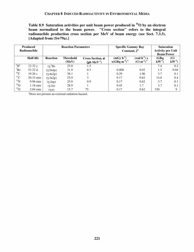
CHAPTER 8 INDUCED RADIOACTIVITY IN ENVIRONMENTAL MEDIA
221
Table 8.9 Saturation activities per unit beam power produced in 16O by an electron beam normalized to the beam power. "Cross section" refers to the integral radionuclide production cross section per MeV of beam energy (see Sect. 7.3.3). [Adapted from (Sw79a).]
Produced Radionuclide
Reaction Parameters Specific Gammy Ray Constant, ΓΓΓΓ
Saturation Activity per Unit
Beam Power
Half-life Reaction Threshold (MeV)
Cross Section, σ σ σ σ (µ(µ(µ(µb MeV-1)
(mGy h-1) x(GBq m-2)-1
(rad h-1) x (Ci m-2)-1
(GBq kW-1)
(Ci kW-1)
3Ha 12.32 y (γ,3H) 25.0 1.5 - - 7.4 0.2 7Be 53.22 d (γ,5n4p) 31.9 0.3 0.008 0.03 1.5 0.04 10C 19.26 s (γ,4n2p) 38.1 1 0.29 1.06 3.7 0.1 11C 20.33 min (γ,3n2p) 25.9 3 0.17 0.62 14.8 0.4 13N 9.96 min (γ,2np) 25.0 0.9 0.17 0.62 3.7 0.1 14O 1.18 min (γ,2n) 28.9 1 0.45 1.7 3.7 0.1 15O 2.04 min (γ,n) 15.7 75 0.17 0.62 330 9
aDoes not present an external radiation hazard.
CHAPTER 8 INDUCED RADIOACTIVITY IN ENVIRONMENTAL MEDIA
222
8.3.2 Water and Geological Media Activation at Proton Accelerators 8.3.2.1 Water Activation At proton and ion accelerators, as with electron accelerators, radioactivity can be produced directly in water as a result of both proton and neutron interactions. Values for some of the relevant cross sections were given in Chapter 7. Equipped with knowledge of the beam energy and information about the energy spectra of neutrons that are present, one can proceed to calculate the activity produced. In general, the most important radionuclides, as is the situation with electron accelerators, result from the interactions of the hadrons with the oxygen present in the water. As before, the production of 3H from the hydrogen present in the water is possible, but is rendered sufficiently improbable due to the small cross sections of both of the thermal neutron capture reactions required to occur sequentially. For such calculations, the production of 3H in water from atoms other than hydrogen is of special importance. Published experimental data of 3H production reactions is surprisingly scarce. Konobeyev and Korovin (Ko93) have developed a method of globally fitting the existing cross section data on the production of 3H due to neutron interactions with a variety of target elements found in soils with the results shown in Fig. 8.4. The results for protons are similar. 8.3.2.2 Geological Media Activation While calculating the production of radionuclides in soil, and in the water it contains, directly from known cross sections has an appeal due to its simplicity, in practice such calculations have been done more frequently by analyzing results obtained using irradiated samples. The work of Borak et al. (Bo72) is of singular importance in this regard. Borak et al. measured the radioactivity produced in soil by high energy hadrons by radiochemical analysis of soil samples irradiated near high energy synchrotrons; the 12 GeV Argonne ZGS and the 28 GeV Brookhaven AGS. The radionuclides 3H, 7Be, 22Na, 45Ca, 46Sc, 48V, 51Cr, 54Mn, 55Fe, 59Fe, and 60Co were identified. Experiments were then performed to determine which radionuclides, and what fractions of them, could be leached by water. This study determined macroscopic production cross sections and ion velocities relative to ground water flow in soil. Of these nuclides, only 3H, 22Na, 45Ca, and 54Mn were observed in leach waters. The 3H was assumed to be all leachable and was measured by driving it out of the sample by baking. Radionuclides with half- lives exceeding 15 days were the only ones considered. The results were based upon the elemental composition of soil given in Table 8.10.
CHAPTER 8 INDUCED RADIOACTIVITY IN ENVIRONMENTAL MEDIA
223
10-1
100
101
102
103
101 102 103 104 105
3 H P
rodu
ctio
n C
ross
Sec
tion
by N
eutro
ns (m
barn
)
Energy (MeV)
Carbon
Oxygen
Magnesium
SiliconCalcium
Iron
Fig. 8.4 Cross sections for the production of 3H due to neutron bombardment of materials commonly
found in soil and rock as a function of neutron energy. The calculations have been performed following the method of Konobeyev and Korovin (Ko93). Results for aluminum are quite similar to those found for silicon and the results for sodium are quite similar to those found for magnesium.
CHAPTER 8 INDUCED RADIOACTIVITY IN ENVIRONMENTAL MEDIA
224
Table 8.10 Composition of soils typical of the Fermilab site. [Adapted from (Bo72).]
Elemental Composition of Soil*
Element Z, Atomic Number % by Weight Silicon 14 14.47 Aluminum 13 2.44 Iron 26 1.11 Calcium 20 7 Magnesium 12 3.79 Carbon 6 5.12 Sodium 11 0.34 Potassium 19 0.814 Oxygen 8 ≈ 64
*The mean moisture percentage was 13.15 + 4.45 % and the mean pH was 7.6 + 0.1. Borak et al. measured specific activities at saturation, Ai , (Bq g-1) which are related to the microscopic cross sections by means of the following equation:
=j
ijji nA σφ , (8.13)
where φ is the flux density (cm-2 s-1), nj is the number density of target nuclei of the jth nuclide (g-1) of the soil sample, and σij (cm2) is the effective cross section for the transformation from target nucleus j to radionuclide i. The summation is taken over the soil constituents. Borak et al. were able to directly measure the summations on the right hand side of Eq (8.13). These summations are the total macroscopic cross sections summed over the soil constituents for each radionuclides of interest. Table 8.11 gives the results of the measurements of the macroscopic cross sections, denoted Σ (cm2 g-1), for each of the radionuclides identified in the various types of soils analyzed. Table 8.11 Macroscopic cross section for soil normalized to unit flux of hadrons with kinetic energies greater than 30 MeV. [Adapted from (Bo72).] Glacial Till Gray Sandy Clay Red Sandy Clay Gray Clay Nuclide ΣΣΣΣ (cm2 g-1) ΣΣΣΣ (cm2 g-1) ΣΣΣΣ (cm2 g-1) ΣΣΣΣ (cm2 g-1)
7Be 2.9 x 10⁻⁴ 3.7 x 10⁻⁴ 3.2 x 10⁻⁴ 2.7 x 10⁻⁴ 51Cr 1.7 x 10⁻⁵ 3.7 x 10⁻⁵ 2.8 x 10⁻⁵ 3.1 x 10⁻⁵ 22Na 2.1 x 10⁻⁴ 2.3 x 10⁻⁴ 2.0 x 10⁻⁴ 1.6 x 10⁻⁴ 54Mn 5.9 x 10⁻⁵ 4.1 x 10⁻⁵ 3.5 x 10⁻⁵ 3.7 x 10⁻⁵ 46Sc 3.0 x 10⁻⁵ 1.3 x 10⁻⁵ 9.6 x 10⁻⁶ 1.1 x 10⁻⁵ 48V 4.1 x 10⁻⁶ 1.1 x 10⁻⁵ 6.7 x 10⁻⁶ 7.4 x 10⁻⁶ 55Fe 9.3 x 10⁻⁵ 1.2 x 10⁻⁴ 7.0 x 10⁻⁵ 2.1 x 10⁻⁴ 59Fe 3.2 x 10⁻⁶ 1.7 x 10⁻⁶ 1.3 x 10⁻⁶ 1.6 x 10⁻⁶ 60Co 3.3 x 10⁻⁵ 1.4 x 10⁻⁵ 1.1 x 10⁻⁵ 1.3 x 10⁻⁵ 45Ca 1.6 x 10⁻⁴ 2.0 x 10⁻⁵ 3.0 x 10⁻⁵ 1.6 x 10⁻⁵ 3H 8.2 x 10⁻⁴ 1.1 x 10⁻³ 3.3 x 10⁻⁴ 5.2 x 10⁻⁴ 3H* 5.9 x 10-3 5.9 x 10⁻³ 4.1 x 10⁻³ 4.4 x 10⁻³
*Cross sections per gram of water in soil.
CHAPTER 8 INDUCED RADIOACTIVITY IN ENVIRONMENTAL MEDIA
225
Borak et al. also obtained data related to the leachabilities of the various elements from the soils studied. Leachability measures the ability of water to remove a given radionuclide from the soil material. It is not related to nuclear properties but rather is related to chemical properties and processes such as ion exchange. The results were reported by Borak et al. as follows:
3H: The leaching process was able to collect all the tritium as measured by a bake-out process. The average value of the macroscopic cross section in soil was found to be 5.1 x 10⁻³ cm2 g-1 of water. An important conclusion is that the tritium will migrate with the same velocity as any other water in the soil.
22Na: Typically 10-20 % of this nuclide was found to be leachable. On average,
it appeared that the migration velocity of this nuclide is approximately 40% of that of water through the soil due to ion exchange processes.
45Ca: At most 5 % of this nuclide was leached from the soil. The migration
velocity was determined to be extremely small. 54Mn: At most 2 % of this nuclide was leached from the soil. It was determined
that this nuclide will not migrate significant distances. Thus, based upon leachability considerations, 3H and 22Na are thus the most important leachable radionuclides that can be produced in environmental media such as soil. One can thus calculate the quantities of radionuclides that might pose a risk to groundwater in the environs of an accelerator. This can be done by using the cross sections directly, or, as demonstrated by Gollon (Go78) for high energy protons, by performing, for example, Monte Carlo calculations in which the total stars (i.e. total inelastic nuclear interactions above some threshold) produced in some volume of earth shielding are determined24. As in Eq. (7.35), the total number of atoms, Ki, of the ith
nuclide that can be produced per star in that same volume is given by
ii
in
KΣ=Σ
, (8.14)
where Σi is, as above, the macroscopic cross section (cm2 g-1) for the ith radionuclide and Σin is the total macroscopic inelastic cross section (cm2 g-1) for soil. Gollon inferred a value of Σin = 1.1 x 10⁻² cm2 g-1 for soil from the results of Borak et al.
24 Some Monte Carlo codes of more recent development can now calculate these quantities directly from the energy-dependent production cross sections. However, given the limited energy dependence at high energies, working with the total stars remains worthwhile as a means to achieve results rapidly, or as a "quality check" on the more complex computations.
CHAPTER 8 INDUCED RADIOACTIVITY IN ENVIRONMENTAL MEDIA
226
Gollon used the following values of Ki for 3H and 22Na, respectively, as selected from Borak's paper for soils peculiar to Fermilab (glacial till):
4
3 2
8.2 100.075
1.1 10K
−
−
×= =×
, and (8.15a)
4
22 2
2.1 100.020
1.1 10K
−
−
×= =×
. (8.15b)
One can then calculate the total number of atoms of radionuclides produced during some time interval in some volume by simply multiplying these factors by the number of stars (or inelastic interactions) in the same volume. The number of atoms then can be converted to activity using the decay constant. The above values of Ki are applicable to soils such as those found at Fermilab. For other soil compositions one may need to use cross sections for producing the radionuclides of interest in various target elements and integrate over the energy spectrum of incident hadrons. Figure 8.5 gives cross sections for producing 22Na by interactions of hadrons with the various elements comprising soil due to Van Ginneken (Va71). This figure is a companion to Fig 8.4. 8.3.3 Regulatory Standards The quantity of ultimate concern, of course, is the resultant concentration in water. The water could be an actual or potential drinking water resource that might well be subject to specific regulatory requirements. The regulations may differ between different governing jurisdictions. The requirements, generally not developed for application to the operations of particle accelerators, need to be understood by facility management personnel. The standards can differ for drinking water supplies and surface water discharges. The allowable concentrations for surface waters may be larger due to the likelihood that such discharges will most certainly be diluted significantly prior to the consumption by individuals. However, in some jurisdictions, this may not be the case. For public drinking water supplies, the U. S. Environmental Protection Agency (CFR76, reaffirmed in CFR00) limits such concentrations to those that would produce an annual dose equivalent of 4 mrem and specifically gives a limit of 20 pCi cm-3 for tritium. An explicit limit for 22Na is not specified by USEPA. For surface water discharges, the U. S. Department of Energy (DOE90) has set forth Derived Concentration Guides, values of concentrations which would result in members of the public each receiving no more than 100 mrem yr-1 should they use such water for their household needs. The DOE DCGs are based upon a more up-to-date dosimetry methodology that results in values of 80 pCi cm-3 for 3H and 0.4 pCi cm-3 for 22Na in drinking water. However, EPA’s explicit limit for 3H in drinking water is considered to be legally preeminent. Table 8.12 lists these concentration limits, Cmax,i. For purposes of this discussion, surface water discharges include those to streams, ponds, etc. while drinking water standards apply to water that could potentially end up in a source of drinking water such as a public, or even private, well. Local jurisdictions can, and in some cases have, applied drinking water standards to all discharges.
CHAPTER 8 INDUCED RADIOACTIVITY IN ENVIRONMENTAL MEDIA
227
10-1
100
101
102
103
101 102 103 104 105
22N
a P
rodu
ctio
n C
ross
Sec
tion
by N
eutro
ns (m
barn
)
Energy (MeV)
SodiumMagnesium
Aluminum
Silicon Calcium
Iron
Fig. 8.5 Cross sections for the production of 22Na due to neutron bombardment of materials commonly
found in soil and rock as a function of neutron energy. Results for potassium are quite similar to those found for calcium. [Adapted from (Va71).]
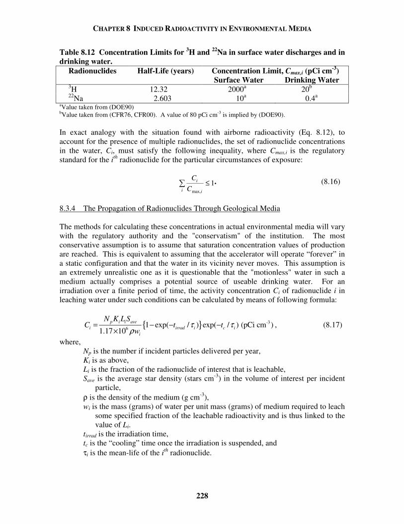
CHAPTER 8 INDUCED RADIOACTIVITY IN ENVIRONMENTAL MEDIA
228
Table 8.12 Concentration Limits for 3H and 22Na in surface water discharges and in drinking water.
Radionuclides Half-Life (years) Concentration Limit, Cmax,i (pCi cm-3) Surface Water Drinking Water
3H 12.32 2000a 20b
22Na 2.603 10a 0.4a
aValue taken from (DOE90) bValue taken from (CFR76, CFR00). A value of 80 pCi cm-3 is implied by (DOE90). In exact analogy with the situation found with airborne radioactivity (Eq. 8.12), to account for the presence of multiple radionuclides, the set of radionuclide concentrations in the water, Ci, must satisfy the following inequality, where Cmax,i is the regulatory standard for the ith radionuclide for the particular circumstances of exposure:
CC
i
ii max, ≤ 1. (8.16)
8.3.4 The Propagation of Radionuclides Through Geological Media The methods for calculating these concentrations in actual environmental media will vary with the regulatory authority and the "conservatism" of the institution. The most conservative assumption is to assume that saturation concentration values of production are reached. This is equivalent to assuming that the accelerator will operate “forever” in a static configuration and that the water in its vicinity never moves. This assumption is an extremely unrealistic one as it is questionable that the "motionless" water in such a medium actually comprises a potential source of useable drinking water. For an irradiation over a finite period of time, the activity concentration Ci of radionuclide i in leaching water under such conditions can be calculated by means of following formula:
-36 1 exp( / ) exp( / ) (pCi cm )
1.17 10p i i ave
i irrad i c ii
N K L SC t t
wτ τ
ρ= − − −
×, (8.17)
where, Np is the number if incident particles delivered per year, Ki is as above, Li is the fraction of the radionuclide of interest that is leachable, Save is the average star density (stars cm-3) in the volume of interest per incident
particle, ρ is the density of the medium (g cm-3), wi is the mass (grams) of water per unit mass (grams) of medium required to leach
some specified fraction of the leachable radioactivity and is thus linked to the value of Li.
tirrad is the irradiation time, tc is the “cooling” time once the irradiation is suspended, and τi is the mean-life of the ith radionuclide.
CHAPTER 8 INDUCED RADIOACTIVITY IN ENVIRONMENTAL MEDIA
229
The constant in the denominator contains the unit conversions needed to yield results in pCi cm-3. For a given medium, the ratio Li/wi should be determined by measurements specific to the local media. An important quantity is the effective porosity, p, which represents the volume fraction of the material that is available to water movement. It is given by p = ρwi. (8.18) The effective porosity is essentially equal to the pore volume of the material for soils but for consolidated materials (i.e., rock) it does not include sealed pores through which movement does not occur. This provides a means by which “worst case” estimates may be made. For realistic estimates some method of taking into account water movement must be used. At Fermilab, a simple model allowing for some movement and further dilution of water was employed for many years (Go78). In this model, called the single resident model for reasons that are obvious, the vertical migration of water was assumed to be 2.2 m yr-1. In the standard clays present at Fermilab, this velocity is likely conservative (i.e., large) by at least an order of magnitude. Its use crudely allowed for the presence of cracks and fissures through which more rapid propagation of water might be possible. The tritium vertical velocity was taken to have this value while the results obtained by Borak et al. (Bo72) were used to obtain a lesser value of about 1.0 m yr-1 for 22Na. Only the leachable fraction of the 22Na is included. The procedure then allowed for decay during the downward migration of the total inventory of radionuclides produced in one year, integrated over the entire volume of the irradiated material, to the highest aquifer below the location of the irradiation. At that point, it was assumed that the radionuclides were rapidly transported horizontally to a shallow well where it was presumed that the flow of water collecting the radionuclides is entirely used by a single user who consumes a volume of 150 liters per day. This value, a minimal one, was taken from results achieved by municipalities that have needed to ration public water consumption during conditions of severe drought. Thus the annual production, as transported vertically, was diluted into the 5.5 x 107 cm3 yr-1 that this represents. This simple model is generally conservative but it does, in fact, neglect that fact that the water movement may not be uniform from year-to-year. It also did not take advantage of the fact that the radionuclides are initially distributed over a considerable volume as they are produced. It is clear that better methods are warranted and a better model has been developed for use at Fermilab (Ma93). The concentration model now in use at Fermilab calculates the production of the radionuclides of concern in accordance with Eq. (8.17). Variations of this approach are used at most large accelerators. The result, then, provides an initial concentration that is available for further migration, decay, and dilution. The concentration after migration is then calculated by using up-to-date modeling techniques to calculate the reduction in the concentration due to dilution, diffusion, and radioactive decay. At the point of concern, usually the location of an aquifer producing water suitable for consumption as a supply of drinking water, the concentrations calculated are then substituted into Eq. (8.16) in order to determine if a shielding design is adequate.
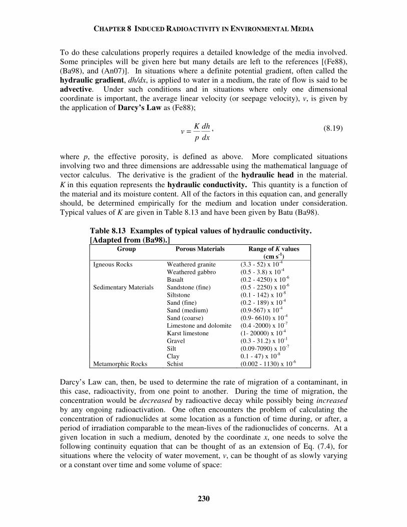
CHAPTER 8 INDUCED RADIOACTIVITY IN ENVIRONMENTAL MEDIA
230
To do these calculations properly requires a detailed knowledge of the media involved. Some principles will be given here but many details are left to the references [(Fe88), (Ba98), and (An07)]. In situations where a definite potential gradient, often called the hydraulic gradient, dh/dx, is applied to water in a medium, the rate of flow is said to be advective. Under such conditions and in situations where only one dimensional coordinate is important, the average linear velocity (or seepage velocity), v, is given by the application of Darcy’s Law as (Fe88); v
Kp
dhdx
= , (8.19)
where p, the effective porosity, is defined as above. More complicated situations involving two and three dimensions are addressable using the mathematical language of vector calculus. The derivative is the gradient of the hydraulic head in the material. K in this equation represents the hydraulic conductivity. This quantity is a function of the material and its moisture content. All of the factors in this equation can, and generally should, be determined empirically for the medium and location under consideration. Typical values of K are given in Table 8.13 and have been given by Batu (Ba98).
Table 8.13 Examples of typical values of hydraulic conductivity. [Adapted from (Ba98).]
Group Porous Materials Range of K values (cm s-1)
Igneous Rocks Weathered granite (3.3 - 52) x 10-4 Weathered gabbro (0.5 - 3.8) x 10-4 Basalt (0.2 - 4250) x 10-6 Sedimentary Materials Sandstone (fine) (0.5 - 2250) x 10-6 Siltstone (0.1 - 142) x 10-8 Sand (fine) (0.2 - 189) x 10-4 Sand (medium) (0.9-567) x 10-4 Sand (coarse) (0.9- 6610) x 10-4 Limestone and dolomite (0.4 -2000) x 10-7 Karst limestone (1- 20000) x 10-4 Gravel (0.3 - 31.2) x 10-1 Silt (0.09-7090) x 10-7 Clay 0.1 - 47) x 10-8 Metamorphic Rocks Schist (0.002 - 1130) x 10-6
Darcy’s Law can, then, be used to determine the rate of migration of a contaminant, in this case, radioactivity, from one point to another. During the time of migration, the concentration would be decreased by radioactive decay while possibly being increased by any ongoing radioactivation. One often encounters the problem of calculating the concentration of radionuclides at some location as a function of time during, or after, a period of irradiation comparable to the mean-lives of the radionuclides of concerns. At a given location in such a medium, denoted by the coordinate x, one needs to solve the following continuity equation that can be thought of as an extension of Eq. (7.4), for situations where the velocity of water movement, v, can be thought of as slowly varying or a constant over time and some volume of space:
CHAPTER 8 INDUCED RADIOACTIVITY IN ENVIRONMENTAL MEDIA
231
),(),( txiQw
iLtxiCix
iCv
tiC
i′=+
∂∂
+∂
∂λ , (8.20)
where all variables are as in Eq. (8.17) with the refinements that λi is the decay constant of the ith radionuclide, x is the spatial coordinate, t is the time, iw′ is the water content of the media per unit volume of media. The quantity Qi(x,t) represents the production of the ith radionuclide and is equivalent to the factor NpSave/(1.17 x 106ρ) in Eq. (8.17). It includes any time-dependence in the delivery of beam. The middle term in the left-hand side of the equation takes care of movement from a point of one concentration to another at the seepage velocity v. As seen elsewhere in this text, one can commonly describe the spatial dependence of the production factor in a thick shield as an exponential function; )−= xtQtxQ oii ξexp()(),( . (8.21) Mokhov (Mo97) has solved this equation for the typical initial conditions of Ci(x,0)=0 and x > 0, t > 0.
In general, 0
( , ) ( , ) exp( )i
i ii
tLC x t dt Q x vt t t
wλ′ ′ ′ ′= − − , (8.22)
and for an exponential spatial dependence as in Eq. (8.21) this becomes:
]1))[exp(exp(1
)(),( −−= τηξη i
ii
ioii x
wL
tQtxC ,
with ηi = ξv - λi ,
τ = t for t < x/v, and τ = x/v for t > x/v. (8.23)
Ci(x,t) has a maximum at xi,max given by,
,max
ln
1
i
i
i
i
vv
xv
ξλξλλ
= −−
. (8.24)
CHAPTER 8 INDUCED RADIOACTIVITY IN ENVIRONMENTAL MEDIA
232
In using these results, one must take care that the algebraic signs of the coordinates x relative to that of v are properly taken into account. In situations where the seepage velocity is extremely slow, diffusion becomes the dominant mechanism for water flow and dilution. Mathematically, a second partial derivative with respect to the spatial coordinate is added to Eq. (8.20). Examples are provided by Fetter (Fe88). Computer software has been written to address this topic such as the one produced by Sudicky et al. (Su88). As a further example of methodologies that can be employed in solving such problems, Jackson (Ja87) has estimated the dilution for a shallow uncased well in an aquifer a distance, r, from a beam loss point also in the aquifer. The loss point was assumed to be within the drawdown zone of the well. This was performed for a simple geology that involved a single uniform stratum of earth above some level of impervious stratum. Fig. 8.6 shows the situation described by this model. Here, a given well is modeled by using the profile of the depth of water, h(r), as a function of r. h(r) is determined by the depth of a test well at radius, r, from the well under consideration and represents the hydraulic potential. The well is assumed to supply a volume, Q, of water per day. The flux of water is determined by the gradient relation, equivalent to Darcy’s Law;
S kdh r
drr = ( ) , (8.25)
where Sr is the inward flux at radius r and k is a constant with dimensions of volume per unit time per unit area and is characteristic of the soil. Conservation of water yields the steady-state equation;
2( )
2 ( ) 2(ln )r
dh d hQ rh r S rkh k
dr d rπ π π= = = . (8.26)
The quantity 2dh
rhdr
π corresponds to the rate of change of volume of the cylindrical
shell of height, h, (i.e., the hydraulic head) with respect to r. This equation has the solution;
22 )( ln oo
hrhkrr
Q −=
π , (8.27)
where ro is the radius of the well and ho is the height of water above the impervious stratum at the well. If H is the depth of the impervious layer below the water table in a asymptotic region unperturbed by any wells, the radius of influence R of the well can be defined by the relation;
QhHk
rR o
o
22 ln
−=
π . (8.28)
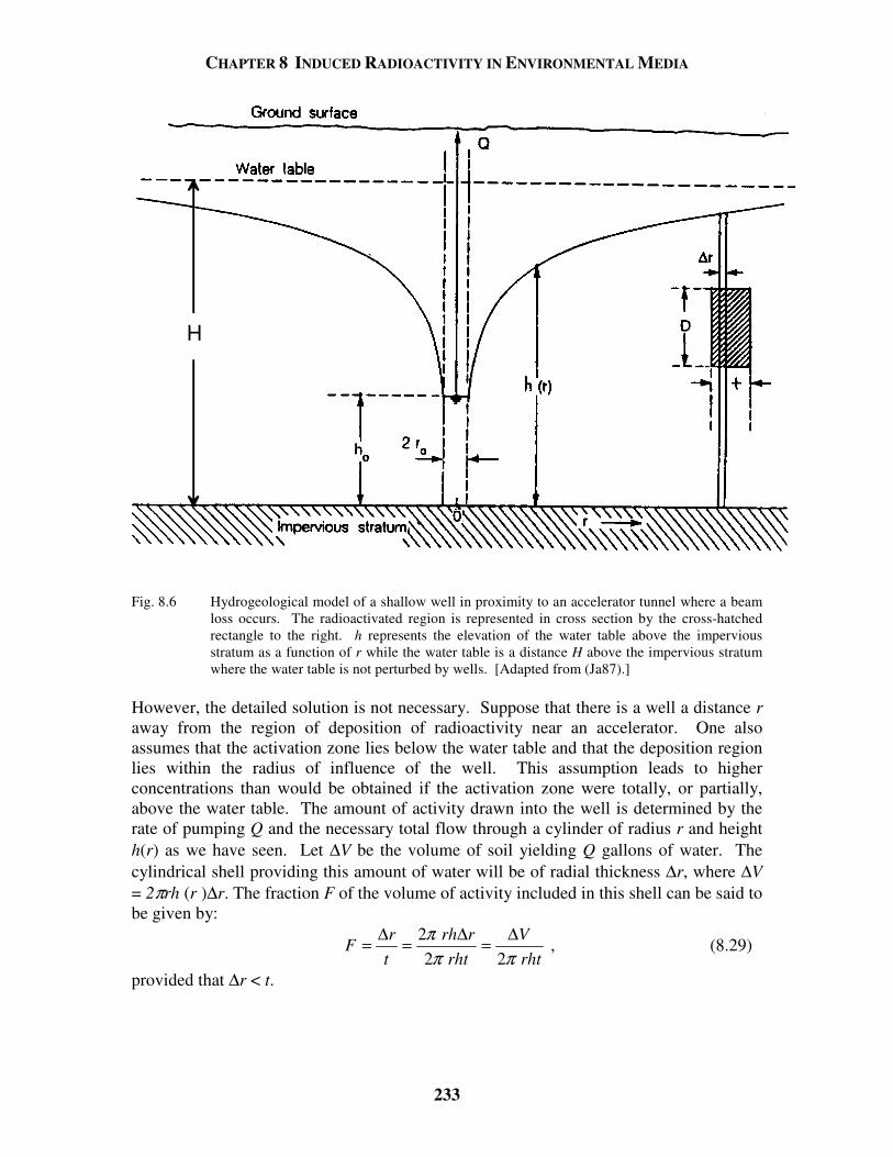
CHAPTER 8 INDUCED RADIOACTIVITY IN ENVIRONMENTAL MEDIA
233
H
Fig. 8.6 Hydrogeological model of a shallow well in proximity to an accelerator tunnel where a beam
loss occurs. The radioactivated region is represented in cross section by the cross-hatched rectangle to the right. h represents the elevation of the water table above the impervious stratum as a function of r while the water table is a distance H above the impervious stratum where the water table is not perturbed by wells. [Adapted from (Ja87).]
However, the detailed solution is not necessary. Suppose that there is a well a distance r away from the region of deposition of radioactivity near an accelerator. One also assumes that the activation zone lies below the water table and that the deposition region lies within the radius of influence of the well. This assumption leads to higher concentrations than would be obtained if the activation zone were totally, or partially, above the water table. The amount of activity drawn into the well is determined by the rate of pumping Q and the necessary total flow through a cylinder of radius r and height h(r) as we have seen. Let ∆V be the volume of soil yielding Q gallons of water. The cylindrical shell providing this amount of water will be of radial thickness ∆r, where ∆V = 2πrh (r )∆r. The fraction F of the volume of activity included in this shell can be said to be given by:
rhtV
rhtrrh
tr
F 2 2
2ππ
π ∆=∆=∆= , (8.29)
provided that ∆r < t.
CHAPTER 8 INDUCED RADIOACTIVITY IN ENVIRONMENTAL MEDIA
234
If the activated region contains leachable activity, A (either total activity or that of a particular radionuclide of interest), the corresponding specific activity, a, in water drawn from the well is thus given by
Apf
DtrA
VpthrV
VpA
FQA
Fa 2
111 2 ππ
=
∆
∆=∆
== , (8.30)
where f = D/h is the fraction of the total height of the cylindrical shell occupied by the activated region and p is the effective porosity of the soil. The pumping volume Q is implicit in f. Porosity values vary considerably but in general are in the range of 0.2 < p < 0.35. (8.31) Thus, this formula may be used to obtain an estimate of the specific activity as a function of distance from the well, although it is perhaps not too useful for applications to beam losses far from the well. By definition, f < 1 and the lower value of porosity can be used to obtain upper limit estimates of the concentration. It must be emphasized that this model depends upon uniformity of water conduction by the strata. The presence of cracks, voids, so-called “sand lenses”, or more complex geological strata can, of course, provide much more rapid movement that is not well-described by this simple model.
CHAPTER 8 INDUCED RADIOACTIVITY IN ENVIRONMENTAL MEDIA
235
Problems
1. A 20 m long air gap has a beam of 1012 s-1 of high energy protons passing through it. First, calculate the production rate of 11C in the gap at equilibrium if one approximates air in the gap by nitrogen and assumes σ (11C) = 10 mb. Assume that there are no significant losses of beam by interaction after checking to see that this assumption is, in fact, true. Table 1.2 contains helpful information.
a) If the air gap is in a 10 x 10 x 20 meter3 enclosure with no ventilation, calculate
the equilibrium concentration of 11C in the room (in units of µCi m-3) assuming extremely rapid mixing (i.e., no time allowed for decay while mixing occurs) of the enclosed air. Compare the concentration with the derived air concentration values in Table 8.6 and calculate, using simple scaling, the dose equivalent to a worker who spends full time in this room. (This is a purely hypothetical scenario due to the much larger hazards due to such an intense direct beam!)
b) Calculate the concentration if two (2) air changes hr-1 are provided. c) Assume the exhaust of the ventilation described in part "b" is through a 10 cm
radius stack 25 m tall. Calculate the air speed in the stack, and the emission rate in Ci s-1. Then using Cember's version of Sutton's equation for tall stacks to estimate the concentration directly downwind at ground level, and hence the dose equivalent 1 km away with moderately stable meteorological conditions and an average wind speed of 10 km hr-1.
d) Perform the same calculation requested in "c" using the more general version of
Sutton's equation appropriate to short stacks and assume the stack height to be 3 meters. All other conditions of the problems are the same as in "c".
2. In soil conditions similar to those at Fermilab, a volume of soil around a beam
absorber approximately 10 m wide by 10 m high by 20 m long is the scene of a star production rate (averaged over the year) of 0.02 stars proton-1 at a beam intensity of 1012 protons s-1.
a) Calculate the annual production of 3H (t1/2 = 12.3 years), the saturated activity (in
Bq & Ci), and the average saturated specific activity in the above volume's water (assume 10% water content by volume).
b) Use the older Fermilab single residence model to calculate the concentration at
the nearest well. Assume the activation region (beam loss point) is 50 m above the aquifer and the usual migration velocities.
c) "Conservatively" apply the "Jackson Model" to estimate the concentration at a
well 100 meters distant from the center of the activation region.
CHAPTER 8 INDUCED RADIOACTIVITY IN ENVIRONMENTAL MEDIA
236
3. The method of accounting for ventilation presented in Section 8.2.2 can readily be generalized to include other mechanisms which “remove” airborne radionuclides such as absorption, filtration, etc. Assume that an arbitrary total number “j” of such mechanisms are present and that the irradiation has gone on sufficiently long to have come to equilibrium between the production of radionuclides and all modes of removal. Following termination of the irradiation, determine the fraction of the total activity that is removed from the air volume by each of the “j” mechanisms. It is safe to assume that all the atoms of the radionuclide produced are removed by one of the processes. The solution of this problem has some importance for the more long-lived radionuclides for it leads to a method of estimating the total activity expected to be found on, say, filter media.
CHAPTER 9 RADIATION PROTECTION INSTRUMENTATION AT ACCELERATORS
237
9.1 Introduction In this chapter instruments and dosimeters currently used in the environment of particle accelerators to measure and characterize the radiation fields are discussed. The emphasis here is on instrumentation that addresses those aspects of accelerator radiation fields that pose special problems that are somewhat unique to this branch of radiation protection. Thomas and Stevenson (Th88) and Swanson and Thomas (Sw90) also discuss these matters. Cember (Ce69) has also described the basics of radiation measurement instrumentation quite well. Knoll (Kn79) has written an excellent detailed treatise on this subject. Virtually all particle detection techniques that have been devised by physicists have to some degree been employed in radiation measurements at accelerators. Furthermore, the specialized instruments used to characterize the accelerator radiation fields are commonly found to be of use to the researcher in the understanding of experiment “backgrounds”. The radiation protection practitioner needs to be able to astutely determine which techniques, including those in use in the physics experiments, can be applied to problems of practical interest in radiation protection. 9.2 Counting Statistics Many of the detection techniques employed to measure radiation fields are directly, or indirectly, dependent upon the counting of individual events such as the passage of charged particles through some medium or the decay of some particle or radionuclide. Cember (Ce69) has given a good summary of counting statistics that is largely repeated here. Radioactive decays are randomly occurring events having a sampling distribution that is correctly described by the binomial distribution given by the following expansion:
( )p q p np qn n
p qn n n
p qn n n n n+ = + + − + − − +− − −1 2 2 3 312
1 23
( )!
( )( )!
...+, (9.1)
where p is the mean probability for occurrence of an event, q is the mean probability of non-occurrence of the event so that p + q = 1, and n is the number of chances of occurrence. The probability of exactly n events occurring is given by the first term, the probability of (n - 1) events is given by the second term, etc. For example, in the throwing of a dice, the probability of throwing a "one" is 1/6 and the probability of throwing a "one" 3 times in a row (n = 3) is pn = (1/6)3 = 1/216. (9.2) In three throws, the probabilities of throwing 2 "ones", 1 "one" and no "ones" are given by the 2nd, 3rd, and 4th terms of the expansion; 15/216, 75/216, and 125/216, respectively.
CHAPTER 9 RADIATION PROTECTION INSTRUMENTATION AT ACCELERATORS
238
This distribution becomes essentially equivalent to the normal or Gaussian distribution when n has an approximate value of at least 30. The Gaussian distribution is as follows:
[ ]p n n n( ) exp ( ) / ( )= − −12
22 2
σ πσ , (9.3)
where p(n) is the probability of finding exactly n, n is the mean value, and σ in this context is the standard deviation and not a reaction cross section. Radioactive decays or particle reactions can often be characterized as highly improbable events. For such “rare” events, the binomial distribution approaches the Poisson distribution. In this distribution, the probability of obtaining n events if the mean value is n , is given by
( )
p nn
n
n n( )
!=
−e. (9.4)
For example consider 10-3 µCi of activity. For this, n = 37 decays sec-1. The probability of exactly observing this number of events in any one second is
( )
p( )!
3737
37
37 37=
−e. (9.5)
One can apply Stirling's approximation to evaluate the factorial;
n
en
nn
= 2! π , (9.6)
where e is the Naperian base (e = 2.718…). Thus p (37) = 0.066. As in the case of the normal distribution, 68 % of the events would lie within one standard deviation of the mean, 96 % of the events would lie within 2 standard deviations of the mean, etc. For the Poisson distribution, the standard deviation is given by σ = n . (9.7)
The relative error, σ/n, is thus n n .
Often, when dealing with instrumentation, the counting rate is involved. For this quantity the following holds:
rnt
ntr± = ±σ , (9.8)
CHAPTER 9 RADIATION PROTECTION INSTRUMENTATION AT ACCELERATORS
239
where r is the counting rate per unit time, σr is its standard deviation, and t is the counting time during which the rate is measured. The quantity t, for example, could even be the integration time constant of some instrument. It follows that
σ rnt
nt t
rt
= = ⋅ =1. (9.9)
Usually, counts due to various background radiations are present and must be dealt with. The standard deviation of the net counting rate is
σ σ σn g bgg
g
bg
bg
r
t
r
t= + = +2 2 , (9.10)
where the subscripts g refer to the measurement of the gross counting rate while the subscripts bg refer to the measurement of the background counting rate. The time durations of the measurements of the rates rg, and rbg are tg and tbg, respectively. In general, the common statistical tests are valid for Poisson statistics. Another quantity that sometimes becomes important is the resolving time, or dead time, of an instrument. This is the time that the detector, following an event, is incapable of measuring a second event. It is a function of both electronic characteristics and the physical process inherent in the detection mechanism. It can be measured by exposure to two different sources of radiation. In such a measurement, a certain detector has a measured background rate of Rbg and responds to first source alone with a rate R1 and to the second source alone with a rate R2 where both R1 and R2 include the background. When exposed to the two sources simultaneously, the measured rate is R12. The resolving time, τ, is given by (Ce69);
τ =+ − −
− −
R R R R
R R R
bg1 2 12
122
12
22 . (9.11)
In many situations, it is often easier to determine τ from the physical properties of the detection mechanism or from the electronic time constants related to the resolving time in the measurement circuitry. If an instrument has a finite resolving time, τ, and the measured counting rate is Rm, then the "true" counting rate, R, that would be observed with a perfect instrument having a resolving time of zero is given by
1
m
m
RR
R τ=
−. (9.12)
Knoll (Kn79) has provided a very detailed discussion of count rate considerations and the optimization of the counting statistics.
CHAPTER 9 RADIATION PROTECTION INSTRUMENTATION AT ACCELERATORS
240
9.3 Special Considerations for Accelerator Environments There are a number of features of accelerator radiation fields which merit attention in choosing instrumentation or measurement techniques. The most important of these are discussed here. 9.3.1 Large Range of Flux Densities, Absorbed Dose Rates, etc. The dynamic range of quantities to be measured encountered at accelerators may extend from fractional mrem yr-1 found in environmental monitoring and environmental studies to the very large values of absorbed dose, up to megarads (106 rads) or so delivered virtually instantaneously of concern in radiation damage situations25. 9.3.2 Possible Large Instantaneous Values of Flux Densities, Absorbed Dose Rates, etc. Certain accelerators such as linacs, rapid cycle synchrotrons, and "single-turn" extracted beams from synchrotrons can have very low average intensities but have extremely high instantaneous rates. Such circumstances arise at accelerators at high intensities or in situations where the duty factor, the fraction of the time the beam is actually present because of accelerator characteristics, of a high intensity radiation field is small. Thus, the dead time considerations described above must be taken into account or the apparent measured values of radiological quantities such as flux densities or dose rates can be misleadingly low. Some instruments can be completely paralyzed by high instantaneous rates. Thus, the effect of dead time on the instantaneous counting rate that is present needs careful consideration. 9.3.3 Large Energy Domain of Neutron Radiation Fields At any given accelerator capable of producing neutrons, the properties of nuclear interactions make it highly probable that neutrons will be present at all energies from thermal (<En > ≈ 0.025 eV) up to nearly the energy of the beam. As will be discussed shortly, the methods of detection of neutrons vary considerably over this energy domain. Thus the choice of instrumentation is crucial to the success of the measurement. For no other particle type is the energy range of the particles encountered in the accelerator environment so large. Also, for no other particles are the types of effective detection techniques so diverse. 9.3.4 Presence of Mixed Radiation Fields At accelerators, one has to consider that any given radiation field external to shielding is likely to be comprised of a mixture of photons, neutrons, and at high energies and at forward angles, muons and even a multitude of other particles. Interior to shielding, the multiplicity of particle types present can be quite large. Also, virtually all neutron fields
25 It is customary to quantify radiation fields in terms of absorbed dose, rather than dose equivalent, at levels above those encountered in routine personnel protection (≈ 1 rad).
CHAPTER 9 RADIATION PROTECTION INSTRUMENTATION AT ACCELERATORS
241
contain at least some photon component due, at least, to the capture of thermal neutrons by means of (n, γ) reactions. Furthermore, muon fields near proton and ion accelerators commonly contain some neutron component. Thus the choice of instrumentation is somewhat dependent upon what particles are present in addition to the one being measured. In certain situations, the radiation field component that is not of immediate interest can actually mask the one of concern. 9.3.5 Directional Sensitivity Certain instruments intrinsically exhibit directional sensitivity. This feature can be either beneficial or detrimental, depending upon the situation. In all instances, it must be understood. It can lead to underestimates in radiation fields where all particles are not monodirectional. Directional sensitivity can actually be useful in certain circumstances to identify sources of unwanted radiation. 9.3.6 Sensitivity to Features of the Accelerator Environment Other than Ionizing Radiation While the focus of this discussion is on ionizing radiation, other features must be taken into account. The most prominent of these is the presence of radiofrequency radiation (RF) at some locations that can perturb instruments which can act, sometimes rather effectively, as "antennas". Environmental effects such as temperature and humidity can also be important. In addition, one must use caution when attempting radiation measurements in the presence of magnetic fields. Induced eddy currents might be interpreted as radiation-induced ionization. Instruments may become magnetized and meter movements may be damaged or “paralyzed”. Also, devices based on photomultiplier tubes commonly read “zero” in static magnetic fields of even moderate strength because of severe deflections of the low energy electrons within the tubes. 9.4 Standard Instruments and Dosimeters This section will review instruments and dosimeters. Some of these are commonly available from commercial sources. However, commercial instruments should be used with care at accelerator facilities to be sure that their properties are adequate for usage in the particular radiological and physical environment at hand. 9.4.1 Ionization Chambers A basic type of instrument used at accelerators to measure absorbed dose rates is the ionization chamber. Such devices are used at high energy accelerators extensively. They rely on the collection of charge liberated by particles passing through a gas. Some detectors used in physics research now employ liquids, both room temperature and cryogenic, for the ionization medium. A beneficial result from atomic physics is that the energy loss per ion pair, W, is nearly a constant over a number of gases and rather independent of type of charged particle as exhibited by Table 9.1.
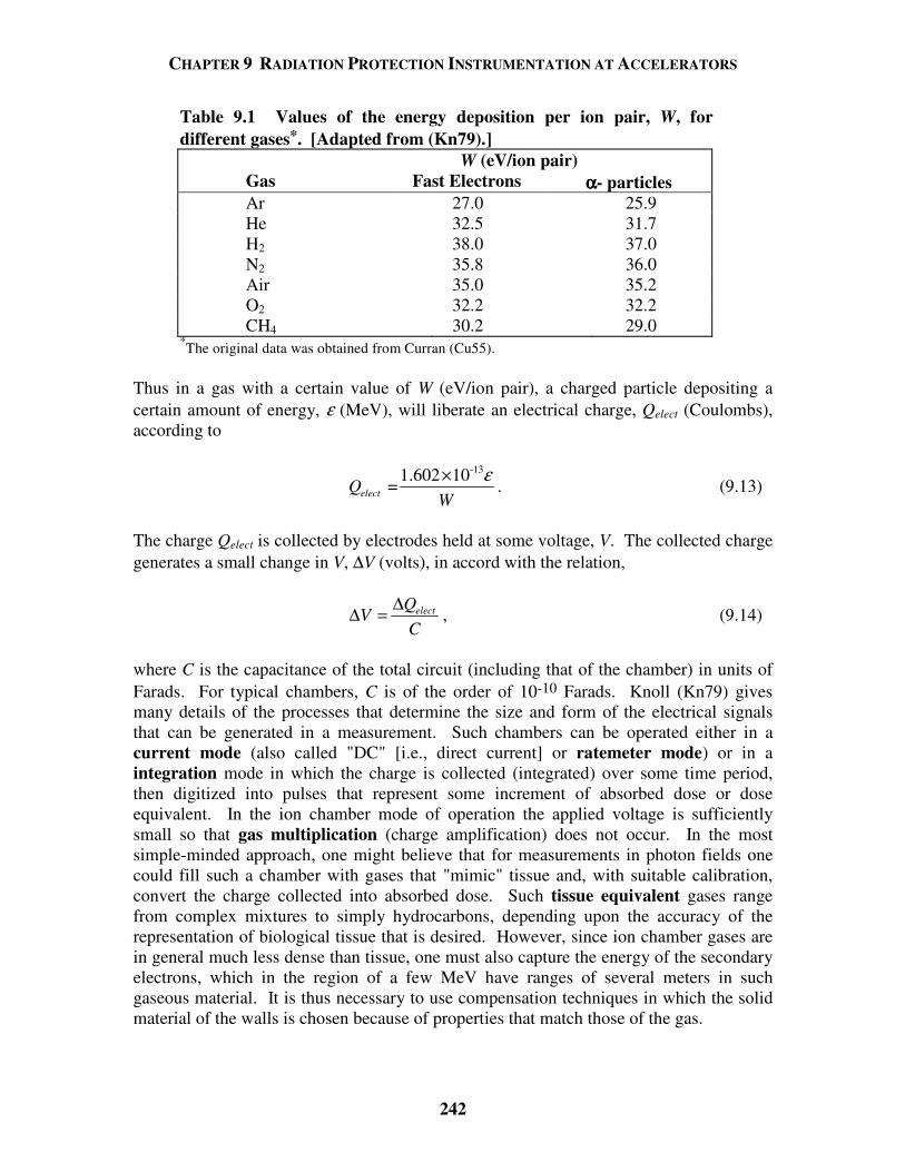
CHAPTER 9 RADIATION PROTECTION INSTRUMENTATION AT ACCELERATORS
242
Table 9.1 Values of the energy deposition per ion pair, W, for different gases*. [Adapted from (Kn79).]
W (eV/ion pair) Gas Fast Electrons αααα- particles Ar 27.0 25.9 He 32.5 31.7 H2 38.0 37.0 N2 35.8 36.0 Air 35.0 35.2 O2 32.2 32.2 CH4 30.2 29.0
*The original data was obtained from Curran (Cu55). Thus in a gas with a certain value of W (eV/ion pair), a charged particle depositing a certain amount of energy, ε (MeV), will liberate an electrical charge, Qelect (Coulombs), according to
-131.602 10
=electQW
ε×. (9.13)
The charge Qelect is collected by electrodes held at some voltage, V. The collected charge generates a small change in V, ∆V (volts), in accord with the relation,
electQV
C∆∆ = , (9.14)
where C is the capacitance of the total circuit (including that of the chamber) in units of Farads. For typical chambers, C is of the order of 10-10 Farads. Knoll (Kn79) gives many details of the processes that determine the size and form of the electrical signals that can be generated in a measurement. Such chambers can be operated either in a current mode (also called "DC" [i.e., direct current] or ratemeter mode) or in a integration mode in which the charge is collected (integrated) over some time period, then digitized into pulses that represent some increment of absorbed dose or dose equivalent. In the ion chamber mode of operation the applied voltage is sufficiently small so that gas multiplication (charge amplification) does not occur. In the most simple-minded approach, one might believe that for measurements in photon fields one could fill such a chamber with gases that "mimic" tissue and, with suitable calibration, convert the charge collected into absorbed dose. Such tissue equivalent gases range from complex mixtures to simply hydrocarbons, depending upon the accuracy of the representation of biological tissue that is desired. However, since ion chamber gases are in general much less dense than tissue, one must also capture the energy of the secondary electrons, which in the region of a few MeV have ranges of several meters in such gaseous material. It is thus necessary to use compensation techniques in which the solid material of the walls is chosen because of properties that match those of the gas.
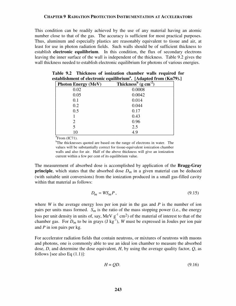
CHAPTER 9 RADIATION PROTECTION INSTRUMENTATION AT ACCELERATORS
243
This condition can be readily achieved by the use of any material having an atomic number close to that of the gas. The accuracy is sufficient for most practical purposes. Thus, aluminum and especially plastics are reasonably equivalent to tissue and air, at least for use in photon radiation fields. Such walls should be of sufficient thickness to establish electronic equilibrium. In this condition, the flux of secondary electrons leaving the inner surface of the wall is independent of the thickness. Table 9.2 gives the wall thickness needed to establish electronic equilibrium for photons of various energies.
Table 9.2 Thickness of ionization chamber walls required for establishment of electronic equilibriuma. [Adapted from (Kn79).]
Photon Energy (MeV) Thicknessb (g cm-2) 0.02 0.0008 0.05 0.0042 0.1 0.014 0.2 0.044 0.5 0.17 1 0.43 2 0.96 5 2.5 10 4.9
aFrom (IC71). bThe thicknesses quoted are based on the range of electrons in water. The values will be substantially correct for tissue-equivalent ionization chamber walls and also for air. Half of the above thickness will give an ionization current within a few per cent of its equilibrium value.
The measurement of absorbed dose is accomplished by application of the Bragg-Gray principle, which states that the absorbed dose Dm in a given material can be deduced (with suitable unit conversions) from the ionization produced in a small gas-filled cavity within that material as follows: D WS Pm m= , (9.15) where W is the average energy loss per ion pair in the gas and P is the number of ion pairs per units mass formed. Sm is the ratio of the mass stopping power (i.e., the energy loss per unit density in units of, say, MeV g-1 cm2) of the material of interest to that of the chamber gas. For Dm to be in grays (J kg-1), W must be expressed in Joules per ion pair and P in ion pairs per kg. For accelerator radiation fields that contain neutrons, or mixtures of neutrons with muons and photons, one is commonly able to use an ideal ion chamber to measure the absorbed dose, D, and determine the dose equivalent, H, by using the average quality factor, Q, as follows [see also Eq (1.1)]: H = QD. (9.16)
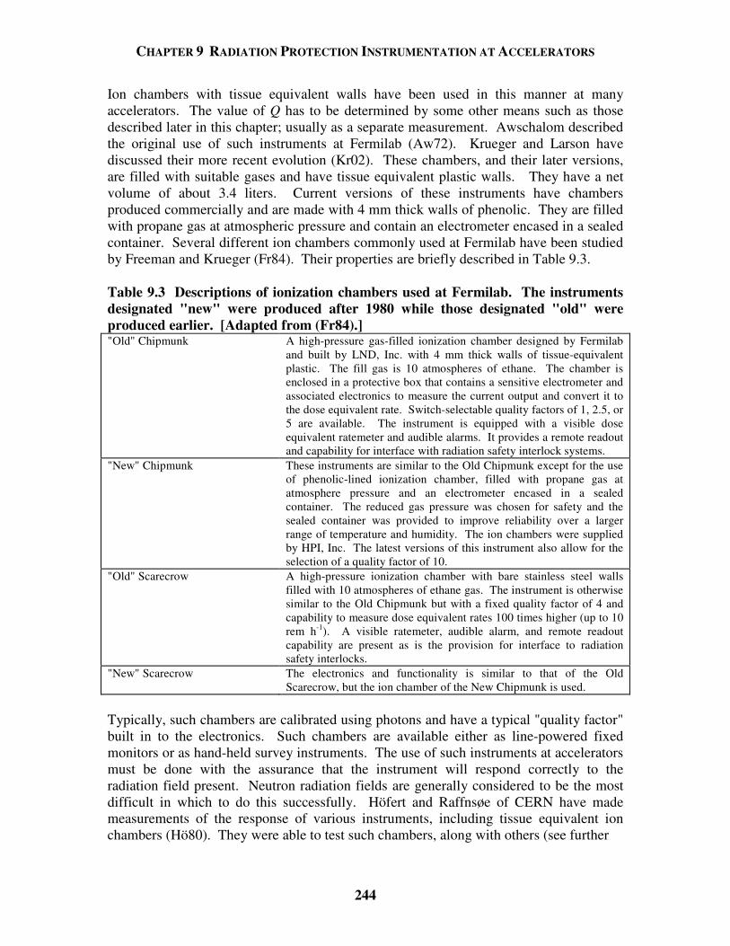
CHAPTER 9 RADIATION PROTECTION INSTRUMENTATION AT ACCELERATORS
244
Ion chambers with tissue equivalent walls have been used in this manner at many accelerators. The value of Q has to be determined by some other means such as those described later in this chapter; usually as a separate measurement. Awschalom described the original use of such instruments at Fermilab (Aw72). Krueger and Larson have discussed their more recent evolution (Kr02). These chambers, and their later versions, are filled with suitable gases and have tissue equivalent plastic walls. They have a net volume of about 3.4 liters. Current versions of these instruments have chambers produced commercially and are made with 4 mm thick walls of phenolic. They are filled with propane gas at atmospheric pressure and contain an electrometer encased in a sealed container. Several different ion chambers commonly used at Fermilab have been studied by Freeman and Krueger (Fr84). Their properties are briefly described in Table 9.3. Table 9.3 Descriptions of ionization chambers used at Fermilab. The instruments designated "new" were produced after 1980 while those designated "old" were produced earlier. [Adapted from (Fr84).] "Old" Chipmunk A high-pressure gas-filled ionization chamber designed by Fermilab
and built by LND, Inc. with 4 mm thick walls of tissue-equivalent plastic. The fill gas is 10 atmospheres of ethane. The chamber is enclosed in a protective box that contains a sensitive electrometer and associated electronics to measure the current output and convert it to the dose equivalent rate. Switch-selectable quality factors of 1, 2.5, or 5 are available. The instrument is equipped with a visible dose equivalent ratemeter and audible alarms. It provides a remote readout and capability for interface with radiation safety interlock systems.
"New" Chipmunk These instruments are similar to the Old Chipmunk except for the use of phenolic-lined ionization chamber, filled with propane gas at atmosphere pressure and an electrometer encased in a sealed container. The reduced gas pressure was chosen for safety and the sealed container was provided to improve reliability over a larger range of temperature and humidity. The ion chambers were supplied by HPI, Inc. The latest versions of this instrument also allow for the selection of a quality factor of 10.
"Old" Scarecrow A high-pressure ionization chamber with bare stainless steel walls filled with 10 atmospheres of ethane gas. The instrument is otherwise similar to the Old Chipmunk but with a fixed quality factor of 4 and capability to measure dose equivalent rates 100 times higher (up to 10 rem h-1). A visible ratemeter, audible alarm, and remote readout capability are present as is the provision for interface to radiation safety interlocks.
"New" Scarecrow The electronics and functionality is similar to that of the Old Scarecrow, but the ion chamber of the New Chipmunk is used.
Typically, such chambers are calibrated using photons and have a typical "quality factor" built in to the electronics. Such chambers are available either as line-powered fixed monitors or as hand-held survey instruments. The use of such instruments at accelerators must be done with the assurance that the instrument will respond correctly to the radiation field present. Neutron radiation fields are generally considered to be the most difficult in which to do this successfully. Höfert and Raffnsøe of CERN have made measurements of the response of various instruments, including tissue equivalent ion chambers (Hö80). They were able to test such chambers, along with others (see further
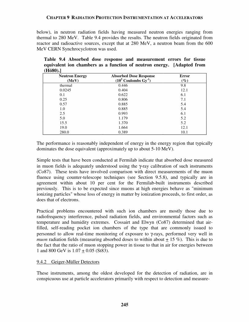
CHAPTER 9 RADIATION PROTECTION INSTRUMENTATION AT ACCELERATORS
245
below), in neutron radiation fields having measured neutron energies ranging from thermal to 280 MeV. Table 9.4 provides the results. The neutron fields originated from reactor and radioactive sources, except that at 280 MeV, a neutron beam from the 600 MeV CERN Synchrocyclotron was used.
Table 9.4 Absorbed dose response and measurement errors for tissue equivalent ion chambers as a function of neutron energy. [Adapted from (Hö80).]
Neutron Energy (MeV)
Absorbed Dose Response (105 Coulombs Gy-1)
Error (%)
thermal 0.446 9.8 0.0245 0.404 12.1 0.1 0.622 6.1 0.25 0.806 7.1 0.57 0.885 5.4 1.0 0.885 5.4 2.5 0.993 6.1 5.0 1.179 5.2 15.5 1.370 5.2 19.0 1.664 12.1 280.0 0.389 10.1
The performance is reasonably independent of energy in the energy region that typically dominates the dose equivalent (approximately up to about 5-10 MeV). Simple tests that have been conducted at Fermilab indicate that absorbed dose measured in muon fields is adequately understood using the γ-ray calibration of such instruments (Co87). These tests have involved comparison with direct measurements of the muon fluence using counter-telescope techniques (see Section 9.5.8), and typically are in agreement within about 10 per cent for the Fermilab-built instruments described previously. This is to be expected since muons at high energies behave as "minimum ionizing particles" whose loss of energy in matter by ionization proceeds, to first order, as does that of electrons. Practical problems encountered with such ion chambers are mostly those due to radiofrequency interference, pulsed radiation fields, and environmental factors such as temperature and humidity extremes. Cossairt and Elwyn (Co87) determined that air-filled, self-reading pocket ion chambers of the type that are commonly issued to personnel to allow real-time monitoring of exposure to γ-rays, performed very well in muon radiation fields (measuring absorbed doses to within about + 15 %). This is due to the fact that the ratio of muon stopping power in tissue to that in air for energies between 1 and 800 GeV is 1.07 + 0.05 (St83). 9.4.2 Geiger-Müller Detectors These instruments, among the oldest developed for the detection of radiation, are in conspicuous use at particle accelerators primarily with respect to detection and measure-
CHAPTER 9 RADIATION PROTECTION INSTRUMENTATION AT ACCELERATORS
246
ment of induced activation and removable induced activity (contamination). In some instances such instruments can be used to identify prompt radiation fields. They are very rugged and remarkably insensitive to environmental effects such as temperature and humidity. However, the typical dead time of 100 µsec or so renders them to be generally useless in fields having high instantaneous rates. 9.4.3 Thermoluminescent Dosimeters (TLDs) Swanson and Thomas (Sw90) and Knoll (Kn79) have provided discussions of the properties of TLDs. These dosimeters are an attractive alternative to photographic film particularly to monitor personnel exposures in β and γ radiation fields. They have also been found to be useful in measuring neutron radiation fields when used as a pair of 6LiF and 7LiF TLDs crystals in the same dosimeter. Such use exploits the fact that the reaction 6Li(n, α)3H has a large thermal neutron cross section of 940 barns (see Section 9.5.1.2) while the 7Li(n, γ)8Li reaction cross section is only 0.037 barns for thermal neutrons. Since a TLD containing either 6Li and 7Li has a comparable efficiency for photon or muon radiation, measurement of the response of the two detectors can, then, be used to determine the dose equivalent due to thermal neutrons in the presence of photons or muons. These reactions provide tools to use in the detection of fast neutrons if moderation is supplied, as will be discussed later. TLDs operate on the principal that some of the radiation liberated by the ionizing particle is "trapped" in band gaps in the crystal lattice. The process is well described by Knoll (Kn79). In particular, ionization elevates electrons from the valence to the conduction band where they are then captured by a "trapping center". At room temperatures, there is only a small probability per unit time that such "trapped" electrons will escape back to the conduction band from the valence band. Thus exposure to radiation continuously populates the traps. "Holes" are similarly trapped in the valence band. When readout of the dose is desired, the crystal is heated and this thermally excites the electrons and holes out of the traps. This process is accompanied by the emission of light that can then be measured as a so-called "glow curve". A number of other materials can function as TLDs; notably CaSO4:Mn, CaF2, and CaF2:Mn. These materials have properties that can be optimized for particular applications. CaF2:Mn is particularly useful for environmental monitoring purposes, where extraordinarily high sensitivity is required. The large numbers of trapped electrons and holes per unit of dose permits sensitivity to absorbed doses as small as 2 x 10⁻⁵ rads. LiF "fades" over time to a lessor degree than most of the other materials at room temperature and its average atomic number is very close to that of tissue, so it is particularly useful for personnel dosimetry. TLDs can give valid results for fields as high as 100 rads. Higher doses can be measured under certain conditions if one takes care to use crystals calibrated in the intense radiation fields since linearity of the response breaks down in the high dose region. These devices exhibit superlinearity. TLDs are not generally susceptible to dose rate problems. However the readout process is intrinsically “destructive” and usually cannot be repeated.
CHAPTER 9 RADIATION PROTECTION INSTRUMENTATION AT ACCELERATORS
247
9.4.4 Nuclear Track Emulsions This discussion is summarized from that of Swanson and Thomas (Sw90). For many years thin (≈ 25 micron) emulsions (NTA) have been used for personal dosimetry in fast neutron fields. The technique is based upon detection of tracks left by proton recoils in the film. The energy range for which these dosimeters are effective is from roughly 0.5 to 25 MeV because below that range the tracks are too short to be read out, while above it there are too few tracks because the (n, p) cross section (elastic scattering, mostly) decreases with energy. However, this energy range is the one that often results in significant neutron dose equivalents at accelerators. The singular important problem with NTA is that the latent image fades and leads to underestimates of the dose equivalent. The fading time can be a short as two weeks. Extreme efforts to keep out the moisture, and experience in dry climates give some indication that this problem can be overcome. Höfert (Hö84b), as has Greenhouse et al. (Gr87), has given a good summary of experience with this dosimeter at accelerators. The dose equivalent range from about 10 mrem to a few hundred mrem is that for which this dosimeter can be expected to perform acceptably. Any technique based upon track formation should not be dependent upon dose rate effects. 9.4.5 Track Etch Dosimeters Swanson and Thomas (Sw90) have discussed the use of such dosimeters. In these detectors, the passage of a charged particle through a dielectric material will result in a trail of damaged molecules in the material. These tracks can be made visible upon etching in a strong acid or base solution. The tracks will be etched at a faster rate than the undamaged portions of the material. As with nuclear emulsions, there is a minimum detectable track length that sets a threshold of about 0.5 MeV on the neutron detection. Such detectors have been reviewed extensively by Griffith and Tommasino (Gr90). Mica, Lexan, and other materials are suitable for this purpose and electronic methods of readout are available. Repeated readouts of the processed tracks are feasible. 9.4.6 CR-39 Dosimeters Swanson and Thomas (Sw90) have provided a discussion of applications of such dosimeters at accelerators. This material, also a “track detector”, has largely replaced NTA as a film dosimeter. It is a casting resin, originally developed for use in eyeglass lenses, that is transparent and is thermoset, rather than thermoplastic. It is the most sensitive of the track detectors and registers recoil protons up to 15 MeV and down to about 0.1 MeV. It is processed either chemically or electrochemically. Repeated readouts of the processed tracks are feasible. The lower limit of detection appears to be superior to that of NTA or Track-Etch (Lexan). There are about 7 x 10³ tracks cm-2 rem-
1, which is adequate, but the sensitivity may be as much as a factor of two lower in high energy spectra. Fading appears to be insignificant. However, natural radon gas can contribute to background readings and the angle of incidence is important.
CHAPTER 9 RADIATION PROTECTION INSTRUMENTATION AT ACCELERATORS
248
9.4.7 Bubble Detectors The use of these detectors at accelerators has also been discussed by Swanson and Thomas (Sw90). The bubble damage polymer detector is an innovative dosimeter that is similar to a bubble chamber in that a liquid whose normal boiling point is below room temperature is kept under pressure. When the pressure is released bubbles form along the path of a charged particle that has traversed it. To enhance the effect, superheated droplets of a volatile liquid are dispersed in a gelatinous medium. There are two types of these detectors that have been developed; one type by Apfel (Ap79) and the other type by Ing (In84). The polymer or gel is supplied in a clear vial. When a neutron interacts in the sensitive material, a bubble is created that expands to optically visible dimensions and can thus be counted. There is no angular dependence but temperature effects must be considered. The Ing detector was reported to exhibit a constant response over the range 15 oC < T < 35 oC. The material can be tailored to match a chosen neutron energy threshold that can be as low as 10 keV or less. Indeed, sets have been prepared with arbitrary thresholds of 0.010, 0.100, 0.500, 1, 3, and 10 MeV. The range of sensitivity can be adjusted to be between 1 and 30 bubbles per mrem, or larger, in a volume of about 4 cm3 and the physical mechanism is not readily sensitive to dose rate effects. Disadvantages include a high unit cost, and the fact that once the vial is opened it is only good for limited periods of time of dose integration. The materials have been successfully used at accelerator facilities. These detectors could not be expected to give accurate results in high dose rates. One can see that no single commercial instrument "solves all problems" simultaneously, especially for neutron fields. The practitioner is encouraged to utilize a variety of instruments, including some of the special techniques discussed below to fully understand the radiation fields. 9.5 Specialized Detectors 9.5.1 Thermal Neutron Detectors Although thermal neutrons are not commonly the major source of neutron dose equivalent at particle accelerators, they are of considerable importance in accelerator radiation protection because of the ability to moderate the fast neutrons (as we shall see below). Furthermore, because some of the most prominent thermal neutron detectors rely upon radioactivation (by neutron capture) as the detection mechanism, they have the advantage that the response is entirely independent of dose rate effects and hence free of dead time effects. An excellent discussion, summarized here, on thermal neutron detectors is given by Knoll (Kn79). At the outset, there are some general features concerning thermal neutrons that need to be recalled. The kinetic energies of thermal neutrons have the familiar relationship as a
CHAPTER 9 RADIATION PROTECTION INSTRUMENTATION AT ACCELERATORS
249
function of temperature given by the Maxwell-Boltzmann distribution:
( )
1/ 23/ 2
2( ) exp
Ef E E
kTkTπ = −
, (9.17)
where f (E) is the fraction of particles, in this case neutrons, of energy E per unit energy interval, the Boltzmann constant k = 1.38 x 10⁻²³ J oK-1 or 8.62 x 10⁻⁵ eV oK-1, and T is the absolute temperature of the gas (oK). The most probable energy, Emp, is given by Emp = kT , (9.18) while the average energy at any given temperature, <E >, is
E kT= 32
. (9.19)
At room temperature T = 293 oK, so that the most probable energy is 0.025 eV. Normally, thermal neutron cross sections are tabulated for this value of kinetic energy. Since thermal neutrons are decidedly nonrelativistic, the most probable velocity, vmp, at T = 293 oK is determined from
2 -11, so that 2200 m s
2mp mp mpE mv kT v= = = . (9.20)
As the neutron energy increases above the thermal value (up to about 1 keV), unless there are resonances present in the cross section, the absorption cross section, σ, has been found to be approximately described by the relation
σ ∝ ∝1 1E v
, (9.21)
that is known as the 1/v law. Thus, within the limits of validity of the 1/v law, one can scale from the tabulated "thermal" cross section, σth, as follows:
( ) mpth
EE
Eσ σ= . (9.22)
Several different nuclear reactions that are initiated by thermal neutrons are used as the basis of detectors. They all involve particular target nuclei and thus the detector materials sometimes depend upon isotopically separated materials to enhance the effectiveness.
CHAPTER 9 RADIATION PROTECTION INSTRUMENTATION AT ACCELERATORS
250
9.5.1.1 Boron-10 The 10B(n, α)7Li reaction is exothermic, having a Q-value [see Eq. (4.1)], Qv,, of 2.792 MeV, and leads either to the ground state of 7Li or its first excited state at 0.482 MeV. The latter occurs for about 94 % of the time when thermal neutrons are incident. Thus, for the dominant transition to the excited state, the reaction imparts about 2.31 MeV to the reaction products. This energy is much larger than the kinetic energy of the incoming thermal neutron. Since energy and momenta must be conserved, for the dominant excited state branch the kinetic energy of the alpha particle, E (α), is 1.47 MeV and, accordingly, E (7Li) = 0.84 MeV. This is because the following must hold: E (7Li) + E (α) = 2.31 MeV, (9.23) due to energy conservation for the excited state branch, if one neglects the very small kinetic energy of the incident thermal neutron. Also, [2m (7Li)E(7Li)]1/2 = [2m(α)E(α)]1/2 . (9.24) holds due to conservation of momentum since the two reaction products emerge in opposite directions. The very small momentum of the thermal neutron is ignored and one recalls that, nonrelativistically, p2 = 2mE, where m denotes the rest mass of the particle. The excited state subsequently decays by emission of a photon. For this reaction, at 0.025 eV, σth = 3837 barns. The relatively large natural abundance of 10B is 20 % compared with 80 % for the other stable isotope, 11B (Se81). The large natural abundance of the crucial isotope makes this reaction very favorable for thermal neutron detection. In addition, material enriched in 10B is readily available. Also the reaction products, and thus their deposited energies, being of short range, are contained in "reasonable" detector configurations. Figure 9.1 gives the cross sections as a function of neutron energy for several of the thermal capture reactions described here, including this one. It is useful that the Boron-10 reaction has a rather featureless cross section and obeys the 1/v law quite well even up to an energy of approximately 0.5 MeV. This reaction has been used principally in BF3 gas in proportional tubes. Proportional counters are somewhat similar in concept to ionization chambers except that the applied electric fields are of sufficient strength to accelerate the initial electrons liberated by the ionization to energies above the thresholds for liberating additional secondary electrons. In typical gases at one atmosphere, this threshold is of the order 106 volts/meter. Under proper conditions, the number of electrons generated in this process can be kept proportional to the energy loss but the number of electrons released (and hence the size of the signal) can be "amplified" by a "gain" of many thousands. In proportional chambers, the region in which these secondary electrons are released is kept small compared to the chamber volume. If the voltage is raised beyond these conditions, then proportionality is lost and the counter enters the Geiger-Mueller mode. Knoll (Kn79) has given a detailed
CHAPTER 9 RADIATION PROTECTION INSTRUMENTATION AT ACCELERATORS
251
exposition on proportional chambers and the gas multiplication process. BF3 is the best of the boron-containing gases as a proportional counter gas because of its "good" properties as a counter gas and also because of the high concentration of boron in the gas molecule. Typical BF3 tubes operate at 2000 to 3000 volts potential with gas ionization multiplications ranging from about 100 to 500. An enriched (96%) BF3 tube can have an absolute detection efficiency of 91 % at 0.025 eV dropping to 3.8 % at 100 eV for neutrons incident upon it. Alternatives with somewhat better gas properties (and cleaner signals) have been achieved by using boron-lined chambers with other gases that have better properties in proportional chambers. 9.5.1.2 Lithium-6 The reaction of interest is 6Li(n, α)3H. For this reaction, Qv = 4.78 MeV. The process leads only to the ground state of 3H. As discussed in connection with the 10B(n, α)7Li reaction, conservation of energy and momentum can be shown to determine the result that E (3H) = 2.73 MeV and E (α) = 2.05 MeV. For incident thermal neutrons, σth = 941 barns (Se81). The natural isotopic abundance of 6Li is about 7.5 %. Figure 9.1 includes the cross section of this reaction as function of neutron kinetic energy. The cross section exhibits a significant resonance at about 3 x 10⁵ eV. The apparent disadvantage of the "small" thermal cross section is offset by the higher Q-value and resultant larger signals. For use in gas counters, no fill gas containing lithium having suitable properties analogous to those of BF3 has been found. Instead, 6Li has been successfully added to scintillators. With the addition of a small amount (< 0.1 % of the total atoms) of europium to LiI [LiI(Eu)], the light output is as much as 35 % of that of a comparable size NaI(Tl) crystal. Such scintillators have a decay time of approximately 0.3 µs. Of course, 6LiF is also in prominent use as a TLD and employs the same nuclear reaction. The TLD can be used in high dose rates, since no instantaneous readout is involved. 9.5.1.3 Helium-3 This nuclide, gaseous at room temperature, is used through the reaction 3He(n, p)3H. The Q-value is 0.765 MeV so that, as for the other reactions, E (p) = 0.574 MeV and E (3H) = 0.191 MeV for incident thermal neutrons. For this reaction, σth = 5327 barns (Se81). Although this isotope of helium can be used directly as a detector gas, it has the disadvantages that the natural abundance is only 0.000138 %, which renders enriched 3He to be rather costly. Also some of the energy can escape the sensitive volume of a detector of reasonable size because of the relatively long range of the emitted proton. Again, the cross section as a function of energy is given in Fig. 9.1. As seen, the cross section is quite "well-behaved". 3He is a reasonable gas for proportional chambers; however no compounds are available since it is a noble gas. In sufficient purity it will work as an acceptable proportional counter gas. Because a proton is the reaction product instead of the short range α-particle, "wall effects" (i.e., effects in which some energy
CHAPTER 9 RADIATION PROTECTION INSTRUMENTATION AT ACCELERATORS
252
escapes the counting gas volume) may be somewhat more severe than for BF3. However, proportional chambers filled with 3H can be operated at much higher pressures than are possible with BF3 and can thus have enhanced detection efficiency.
10-1
100
101
102
103
104
10-2 10-1 100 101 102 103 104 105 106 107
3He(n,p)3H6Li(n,α)3H10B(n,α)7Li
Cro
ss S
ectio
n (b
arns
)
Neutron Energy (eV)
Fig. 9.1 Cross section versus neutron energy for some reactions of interest in neutron detection.
[Adapted from (Kn79).]
CHAPTER 9 RADIATION PROTECTION INSTRUMENTATION AT ACCELERATORS
253
9.5.1.4 Cadmium This discussion would be incomplete without discussing cadmium. Averaged over the naturally-occurring isotopes of cadmium, the thermal neutron capture reaction of form ACd(n, γ)A+1Cd has a cross section σth = 2450 barns. More spectacularly, the reaction 113Cd(n, γ)114Cd has a value of σth = 19910 barns (Se81). 113Cd has a natural abundance of 12.2 %. Thus, even without using enriched material, the thermal neutron cross section is large. This element is not used directly in the detector medium. Rather, it is used to shield other detectors from thermal neutrons because the large cross section results in the absorption of essentially all neutrons with energies less than about 0.4 eV. Hence, one can do measurements with and without the Cd inside of some moderator (see Section 9.5.2) and have a very clear understanding of the thermal component. 9.5.1.5 Silver Awschalom et al. was able to use thermal neutron capture on silver as a basis of a moderated detector (Aw72). As it occurs in nature, silver has two stable isotopes which both capture thermal neutrons via the (n, γ) process; 107Ag (51.8 % natural abundance, σth = 40 barns) and 109Ag (48.2 % natural abundance, σth = 93.5 barns). The average value of σth is 63.6 barns (Se81). While the cross sections are not as large as those of some of the other reactions discussed, the material is readily available and enrichment is not needed. The detector which utilized these capture reactions was a moderated one (see below) in which the output of a Geiger-Mueller tube wrapped with silver that sensed the capture γ-rays was compared with an identical tube wrapped with tin (average mass number = 118.7). Tin has an average value of σth = 0.63 barns and is thus comparatively insensitive to thermal neutrons. The tin-wrapped tube was then used to subtract background due to muons, photons, etc. 9.5.2 Moderated Neutron Detectors As seen above, many neutron reactions tend to have much smaller cross sections in the MeV region than they have in the "thermal" region. Historically, shortly after the discovery of the neutron, it was observed that surrounding a thermal neutron detector with hydrogenous material enhance detection rates exhibited by a "bare" thermal neutron detector placed in the same radiation field. The reason this occurs with hydrogenous materials is because in nonrelativistic elastic scattering, as we have seen before, the fraction of the incident energy, Eo, that can be transferred to the target nucleus after a collision where the target nucleus recoils at angle θ is determined by conservation of momentum and energy to be given by
2
2
)
cos4
Μ+(1=
∆ θME
E
o, (9.25)
where M is the mass of the target nucleus in units where the mass of the neutron is unity.
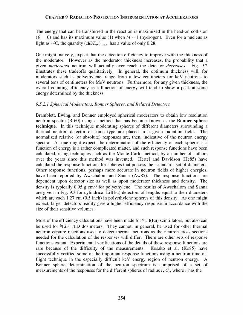
CHAPTER 9 RADIATION PROTECTION INSTRUMENTATION AT ACCELERATORS
254
The energy that can be transferred in the reaction is maximized in the head-on collision (θ = 0) and has its maximum value (1) when M ≈ 1 (hydrogen). Even for a nucleus as light as 12C, the quantity (∆E/Eo )max has a value of only 0.28. One might, naively, expect that the detection efficiency to improve with the thickness of the moderator. However as the moderator thickness increases, the probability that a given moderated neutron will actually ever reach the detector decreases. Fig. 9.2 illustrates these tradeoffs qualitatively. In general, the optimum thickness will, for moderators such as polyethylene, range from a few centimeters for keV neutrons to several tens of centimeters for MeV neutrons. Furthermore, for any given thickness, the overall counting efficiency as a function of energy will tend to show a peak at some energy determined by the thickness. 9.5.2.1 Spherical Moderators, Bonner Spheres, and Related Detectors Bramblett, Ewing, and Bonner employed spherical moderators to obtain low resolution neutron spectra (Br60) using a method that has become known as the Bonner sphere technique. In this technique moderating spheres of different diameters surrounding a thermal neutron detector of some type are placed in a given radiation field. The normalized relative (or absolute) responses are, then, indicative of the neutron energy spectra. As one might expect, the determination of the efficiency of each sphere as a function of energy is a rather complicated matter, and such response functions have been calculated, using techniques such as the Monte Carlo method, by a number of authors over the years since this method was invented. Hertel and Davidson (He85) have calculated the response functions for spheres that possess the "standard" set of diameters. Other response functions, perhaps more accurate in neutron fields of higher energies, have been reported by Awschalom and Sanna (Aw85). The response functions are dependent upon detector size as well as upon moderator thickness and density. The density is typically 0.95 g cm-3 for polyethylene. The results of Awschalom and Sanna are given in Fig. 9.3 for cylindrical LiI(Eu) detectors of lengths equal to their diameters which are each 1.27 cm (0.5 inch) in polyethylene spheres of this density. As one might expect, larger detectors readily give a higher efficiency response in accordance with the size of their sensitive volumes. Most of the efficiency calculations have been made for 6LiI(Eu) scintillators, but also can be used for 6LiF TLD dosimeters. They cannot, in general, be used for other thermal neutron capture reactions used to detect thermal neutrons as the neutron cross sections needed for the calculation of the responses will differ. There are other sets of response functions extant. Experimental verifications of the details of these response functions are rare because of the difficulty of the measurements. Kosako et al. (Ko85) have successfully verified some of the important response functions using a neutron time-of-flight technique in the especially difficult keV energy region of neutron energy. A Bonner sphere determination of the neutron spectrum is comprised of a set of measurements of the responses for the different spheres of radius r, Cr, where r has the
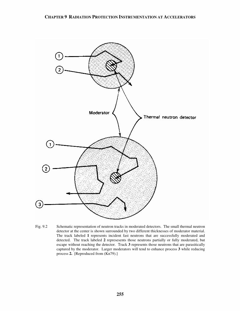
CHAPTER 9 RADIATION PROTECTION INSTRUMENTATION AT ACCELERATORS
255
Fig. 9.2 Schematic representation of neutron tracks in moderated detectors. The small thermal neutron
detector at the center is shown surrounded by two different thicknesses of moderator material. The track labeled 1 represents incident fast neutrons that are successfully moderated and detected. The track labeled 2 represesents those neutrons partially or fully moderated, but escape without reaching the detector. Track 3 represents those neutrons that are parasitically captured by the moderator. Larger moderators will tend to enhance process 3 while reducing process 2. [Reproduced from (Kn79).]
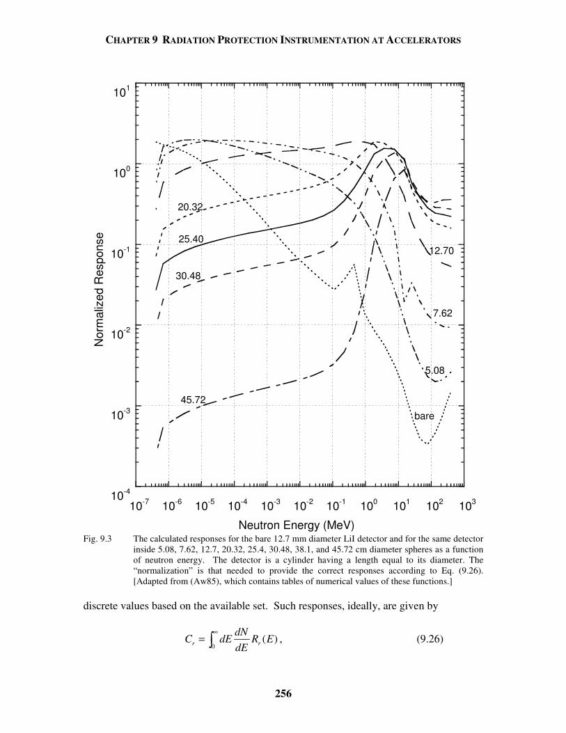
CHAPTER 9 RADIATION PROTECTION INSTRUMENTATION AT ACCELERATORS
256
10-4
10-3
10-2
10-1
100
101
10-7 10-6 10-5 10-4 10-3 10-2 10-1 100 101 102 103
Nor
mal
ized
Res
pons
e
Neutron Energy (MeV)
bare
5.08
7.62
12.70
20.32
25.40
30.48
45.72
Fig. 9.3 The calculated responses for the bare 12.7 mm diameter LiI detector and for the same detector
inside 5.08, 7.62, 12.7, 20.32, 25.4, 30.48, 38.1, and 45.72 cm diameter spheres as a function of neutron energy. The detector is a cylinder having a length equal to its diameter. The “normalization” is that needed to provide the correct responses according to Eq. (9.26). [Adapted from (Aw85), which contains tables of numerical values of these functions.]
discrete values based on the available set. Such responses, ideally, are given by
0
( )r r
dNC dE R E
dE
∞= , (9.26)
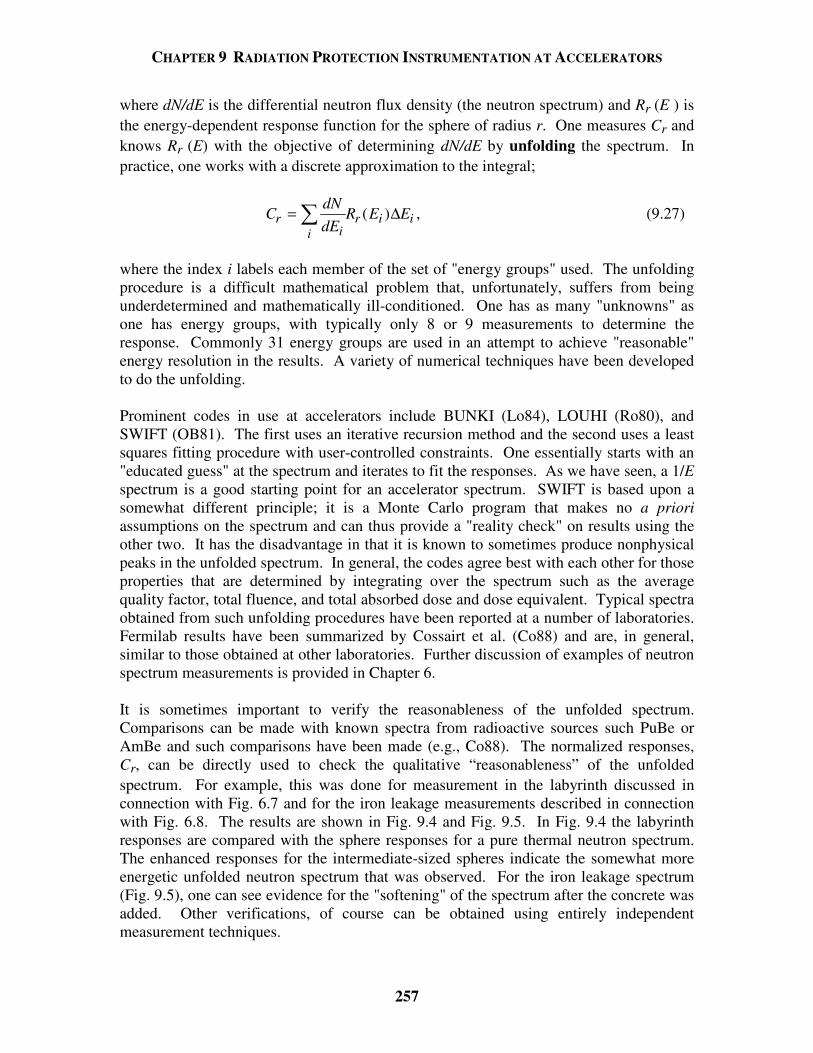
CHAPTER 9 RADIATION PROTECTION INSTRUMENTATION AT ACCELERATORS
257
where dN/dE is the differential neutron flux density (the neutron spectrum) and Rr (E ) is the energy-dependent response function for the sphere of radius r. One measures Cr and knows Rr (E) with the objective of determining dN/dE by unfolding the spectrum. In practice, one works with a discrete approximation to the integral;
CdNdE
R E Erii
r i i= ( )∆ , (9.27)
where the index i labels each member of the set of "energy groups" used. The unfolding procedure is a difficult mathematical problem that, unfortunately, suffers from being underdetermined and mathematically ill-conditioned. One has as many "unknowns" as one has energy groups, with typically only 8 or 9 measurements to determine the response. Commonly 31 energy groups are used in an attempt to achieve "reasonable" energy resolution in the results. A variety of numerical techniques have been developed to do the unfolding. Prominent codes in use at accelerators include BUNKI (Lo84), LOUHI (Ro80), and SWIFT (OB81). The first uses an iterative recursion method and the second uses a least squares fitting procedure with user-controlled constraints. One essentially starts with an "educated guess" at the spectrum and iterates to fit the responses. As we have seen, a 1/E spectrum is a good starting point for an accelerator spectrum. SWIFT is based upon a somewhat different principle; it is a Monte Carlo program that makes no a priori assumptions on the spectrum and can thus provide a "reality check" on results using the other two. It has the disadvantage in that it is known to sometimes produce nonphysical peaks in the unfolded spectrum. In general, the codes agree best with each other for those properties that are determined by integrating over the spectrum such as the average quality factor, total fluence, and total absorbed dose and dose equivalent. Typical spectra obtained from such unfolding procedures have been reported at a number of laboratories. Fermilab results have been summarized by Cossairt et al. (Co88) and are, in general, similar to those obtained at other laboratories. Further discussion of examples of neutron spectrum measurements is provided in Chapter 6. It is sometimes important to verify the reasonableness of the unfolded spectrum. Comparisons can be made with known spectra from radioactive sources such PuBe or AmBe and such comparisons have been made (e.g., Co88). The normalized responses, Cr, can be directly used to check the qualitative “reasonableness” of the unfolded spectrum. For example, this was done for measurement in the labyrinth discussed in connection with Fig. 6.7 and for the iron leakage measurements described in connection with Fig. 6.8. The results are shown in Fig. 9.4 and Fig. 9.5. In Fig. 9.4 the labyrinth responses are compared with the sphere responses for a pure thermal neutron spectrum. The enhanced responses for the intermediate-sized spheres indicate the somewhat more energetic unfolded neutron spectrum that was observed. For the iron leakage spectrum (Fig. 9.5), one can see evidence for the "softening" of the spectrum after the concrete was added. Other verifications, of course can be obtained using entirely independent measurement techniques.
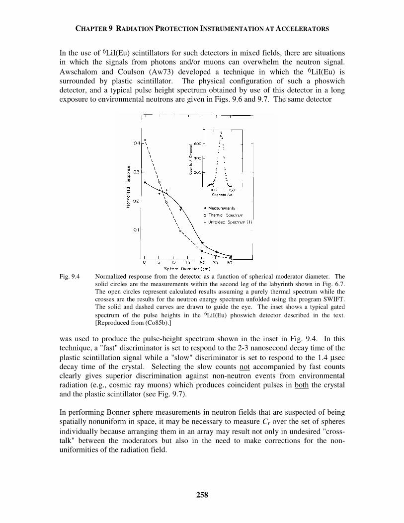
CHAPTER 9 RADIATION PROTECTION INSTRUMENTATION AT ACCELERATORS
258
In the use of 6LiI(Eu) scintillators for such detectors in mixed fields, there are situations in which the signals from photons and/or muons can overwhelm the neutron signal. Awschalom and Coulson (Aw73) developed a technique in which the 6LiI(Eu) is surrounded by plastic scintillator. The physical configuration of such a phoswich detector, and a typical pulse height spectrum obtained by use of this detector in a long exposure to environmental neutrons are given in Figs. 9.6 and 9.7. The same detector
Fig. 9.4 Normalized response from the detector as a function of spherical moderator diameter. The
solid circles are the measurements within the second leg of the labyrinth shown in Fig. 6.7. The open circles represent calculated results assuming a purely thermal spectrum while the crosses are the results for the neutron energy spectrum unfolded using the program SWIFT. The solid and dashed curves are drawn to guide the eye. The inset shows a typical gated spectrum of the pulse heights in the 6LiI(Eu) phoswich detector described in the text. [Reproduced from (Co85b).]
was used to produce the pulse-height spectrum shown in the inset in Fig. 9.4. In this technique, a "fast" discriminator is set to respond to the 2-3 nanosecond decay time of the plastic scintillation signal while a "slow" discriminator is set to respond to the 1.4 µsec decay time of the crystal. Selecting the slow counts not accompanied by fast counts clearly gives superior discrimination against non-neutron events from environmental radiation (e.g., cosmic ray muons) which produces coincident pulses in both the crystal and the plastic scintillator (see Fig. 9.7). In performing Bonner sphere measurements in neutron fields that are suspected of being spatially nonuniform in space, it may be necessary to measure Cr over the set of spheres individually because arranging them in an array may result not only in undesired "cross-talk" between the moderators but also in the need to make corrections for the non-uniformities of the radiation field.
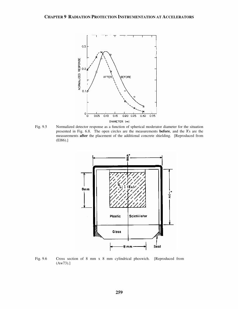
CHAPTER 9 RADIATION PROTECTION INSTRUMENTATION AT ACCELERATORS
259
Fig. 9.5 Normalized detector response as a function of spherical moderator diameter for the situation
presented in Fig. 6.8. The open circles are the measurements before, and the X's are the measurements after the placement of the additional concrete shielding. [Reproduced from (El86).]
Fig. 9.6 Cross section of 8 mm x 8 mm cylindrical phoswich. [Reproduced from (Aw73).]
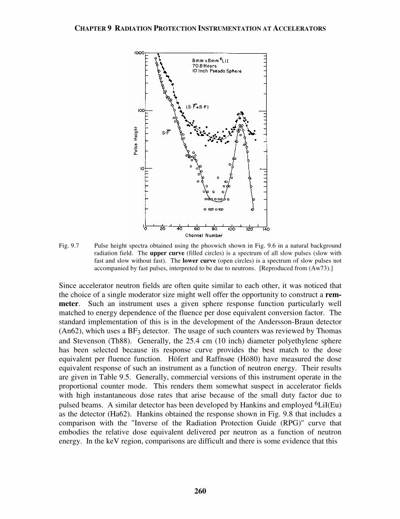
CHAPTER 9 RADIATION PROTECTION INSTRUMENTATION AT ACCELERATORS
260
Fig. 9.7 Pulse height spectra obtained using the phoswich shown in Fig. 9.6 in a natural background
radiation field. The upper curve (filled circles) is a spectrum of all slow pulses (slow with fast and slow without fast). The lower curve (open circles) is a spectrum of slow pulses not accompanied by fast pulses, interpreted to be due to neutrons. [Reproduced from (Aw73).]
Since accelerator neutron fields are often quite similar to each other, it was noticed that the choice of a single moderator size might well offer the opportunity to construct a rem-meter. Such an instrument uses a given sphere response function particularly well matched to energy dependence of the fluence per dose equivalent conversion factor. The standard implementation of this is in the development of the Andersson-Braun detector (An62), which uses a BF3 detector. The usage of such counters was reviewed by Thomas and Stevenson (Th88). Generally, the 25.4 cm (10 inch) diameter polyethylene sphere has been selected because its response curve provides the best match to the dose equivalent per fluence function. Höfert and Raffnsøe (Hö80) have measured the dose equivalent response of such an instrument as a function of neutron energy. Their results are given in Table 9.5. Generally, commercial versions of this instrument operate in the proportional counter mode. This renders them somewhat suspect in accelerator fields with high instantaneous dose rates that arise because of the small duty factor due to pulsed beams. A similar detector has been developed by Hankins and employed 6LiI(Eu) as the detector (Ha62). Hankins obtained the response shown in Fig. 9.8 that includes a comparison with the "Inverse of the Radiation Protection Guide (RPG)" curve that embodies the relative dose equivalent delivered per neutron as a function of neutron energy. In the keV region, comparisons are difficult and there is some evidence that this
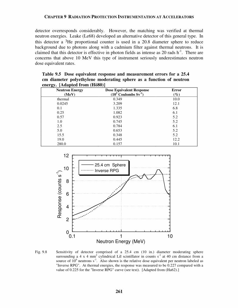
CHAPTER 9 RADIATION PROTECTION INSTRUMENTATION AT ACCELERATORS
261
detector overresponds considerably. However, the matching was verified at thermal neutron energies. Leake (Le68) developed an alternative detector of this general type. In this detector a 3He proportional counter is used in a 20.8 diameter sphere to reduce background due to photons along with a cadmium filter against thermal neutrons. It is claimed that this detector is effective in photon fields as intense as 20 rads h-1. There are concerns that above 10 MeV this type of instrument seriously underestimates neutron dose equivalent rates.
Table 9.5 Dose equivalent response and measurement errors for a 25.4 cm diameter polyethylene moderating sphere as a function of neutron energy. [Adapted from (Hö80)]
Neutron Energy (MeV)
Dose Equivalent Response (105 Coulombs Sv-1)
Error (%)
thermal 0.349 10.0 0.0245 3.209 12.1 0.1 1.335 6.8 0.25 1.082 6.1 0.57 0.923 5.2 1.0 0.745 5.2 2.5 0.784 6.1 5.0 0.653 5.2 15.5 0.348 5.2 19.0 0.445 12.2 280.0 0.157 10.1
0
2
4
6
8
10
12
0.1 1 10
25.4 cm SphereInverse RPG
Res
pons
e (c
ount
s s-1
)
Neutron Energy (MeV) Fig. 9.8 Sensitivity of detector comprised of a 25.4 cm (10 in.) diameter moderating sphere
surrounding a 4 x 4 mm2 cylindrical LiI scintillator in counts s-1 at 40 cm distance from a source of 106 neutrons s-1. Also shown is the relative dose equivalent per neutron labeled as "Inverse RPG". At thermal energies, the response was measured to be 0.227 compared with a value of 0.225 for the "Inverse RPG" curve (see text). [Adapted from (Ha62).]
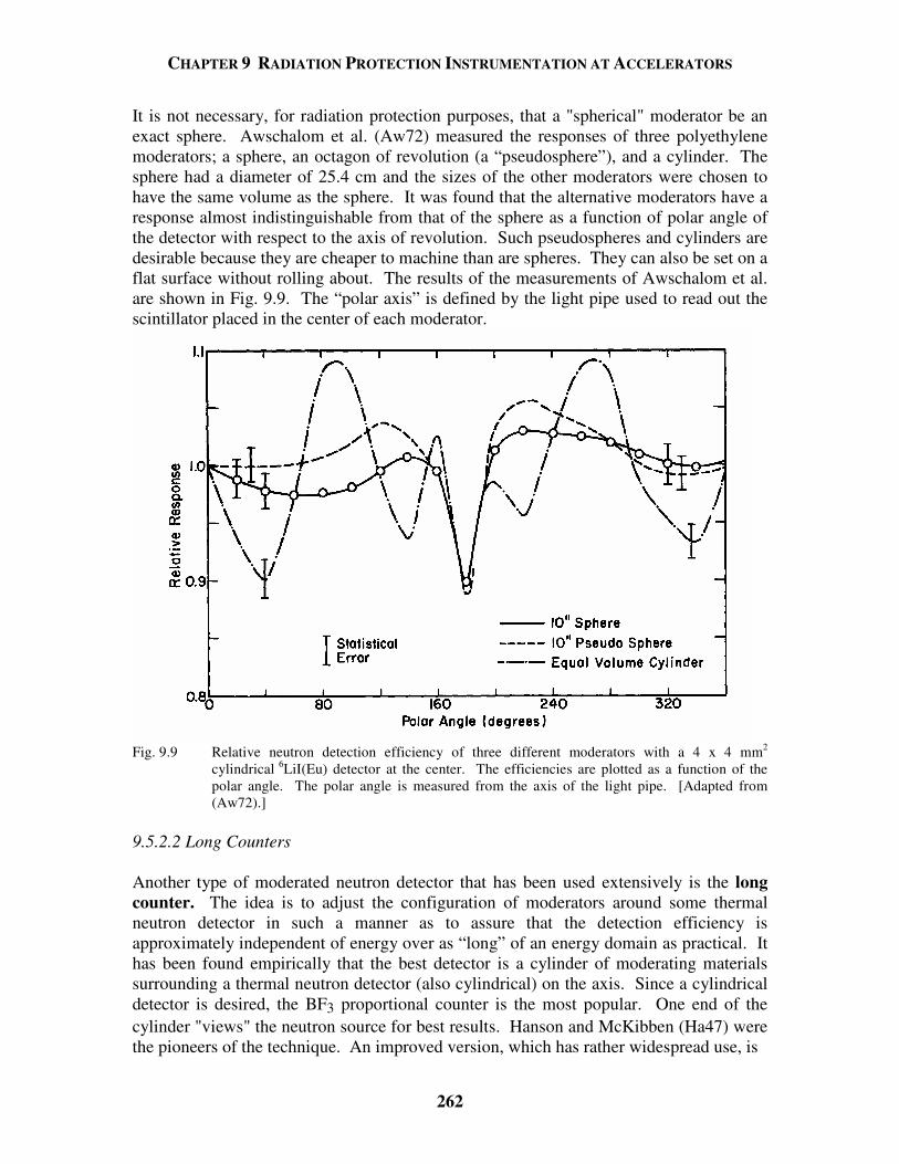
CHAPTER 9 RADIATION PROTECTION INSTRUMENTATION AT ACCELERATORS
262
It is not necessary, for radiation protection purposes, that a "spherical" moderator be an exact sphere. Awschalom et al. (Aw72) measured the responses of three polyethylene moderators; a sphere, an octagon of revolution (a “pseudosphere”), and a cylinder. The sphere had a diameter of 25.4 cm and the sizes of the other moderators were chosen to have the same volume as the sphere. It was found that the alternative moderators have a response almost indistinguishable from that of the sphere as a function of polar angle of the detector with respect to the axis of revolution. Such pseudospheres and cylinders are desirable because they are cheaper to machine than are spheres. They can also be set on a flat surface without rolling about. The results of the measurements of Awschalom et al. are shown in Fig. 9.9. The “polar axis” is defined by the light pipe used to read out the scintillator placed in the center of each moderator.
Fig. 9.9 Relative neutron detection efficiency of three different moderators with a 4 x 4 mm2
cylindrical 6LiI(Eu) detector at the center. The efficiencies are plotted as a function of the polar angle. The polar angle is measured from the axis of the light pipe. [Adapted from (Aw72).]
9.5.2.2 Long Counters Another type of moderated neutron detector that has been used extensively is the long counter. The idea is to adjust the configuration of moderators around some thermal neutron detector in such a manner as to assure that the detection efficiency is approximately independent of energy over as “long” of an energy domain as practical. It has been found empirically that the best detector is a cylinder of moderating materials surrounding a thermal neutron detector (also cylindrical) on the axis. Since a cylindrical detector is desired, the BF3 proportional counter is the most popular. One end of the cylinder "views" the neutron source for best results. Hanson and McKibben (Ha47) were the pioneers of the technique. An improved version, which has rather widespread use, is
CHAPTER 9 RADIATION PROTECTION INSTRUMENTATION AT ACCELERATORS
263
that developed by DePangher and Nichols (DeP66). Figure 9.10 shows the layout of this detector. The length and diameter are both approximately 41 cm and the mass is about 45 kg. It is designed and calibrated for use with the neutrons incident on the "front" face. Perhaps the best calibration data on this device is that of Slaughter and Rueppel (Sl77). They used filtered beams from a reactor (En ≈ keV) as well as monoenergetic neutron beams from (p, n) and (d, n) reactions at accelerators to cover the energy range from 10 keV to 19 MeV. An average of about 3.5 counts/(n cm-2) sensitivity was reported over this energy domain, with deviations of from 5 to 30 per cent from absolute independence of neutron energy. A similar detector has been used to conduct studies of skyshine at Fermilab [(Co85c) and (El86)]. The large peak in the pulse-height spectrum of the BF3 tube from thermal neutron capture (Qv = 2.79 MeV) renders the detector essentially insensitive, with the application of a suitable pulse-height discriminator, to all other radiations. Knoll (Kn79) summarizes results with modified long counters that achieve better uniformity and higher levels of sensitivity over more restricted energy domains. 9.5.3 Activation Detectors As we have seen, certain nuclear reactions have relatively sharp thresholds which can be used to determine portions of a hadron spectrum that exceed it since the "leveling off" of the cross sections are generally well-behaved. In addition to information on reaction thresholds provided in Chapter 7, where referral was made to activation threshold techniques, Table 9.6 summarizes some of the useful reactions along with some pertinent information about threshold detectors that have been found to be useful in practical work. Some of these reactions will be discussed further below. Thomas and Stevenson (Th85 and Th88) provide a list of other reactions that might have useful thresholds. Table 9.6 Important characteristics of various activation detector nuclear reactions.
Detector Reaction Energy Range (MeV)
Half-Life Typical Detector Size
Cross Section-
Peak (mb)
Cross Section-High
Energy(mb)
Particle Detected
sulfur 32S(n,p)32P > 3 14.26 d 4 g disk 500a 10a β-
aluminum 27Al(n,α)24Na > 6 14.95 h 16 - 6600 g 11b 9b γ aluminum 27Al(n,x)22Na > 25 2.603 y 17 g 30b 10b γ plastic scintillator
12C-> 11C > 20 20.33 min 13-2700 g 90b 30b β+, γ
plastic scintillator
12C->7Be > 30 53.22 d 17 g 18b 10b γ
mercury 198Hg->149Tb > 600 4.12 h up to 500 g 2b 1b α,γ gold 197Au->149Tb > 600 4.12 h 0.5 g 1.6b 0.7b α,γ copper Cu->24Na > 600 14.95 h 580 g 4c 3.9c γ copper Cu->52Mn > 70 5.59 d 580 g 5c 4.6c γ copper Cu->54Mn > 80 312.1 d 580 g 11c 11c γ
aSwanson and Thomas (Sw90) bBarbier (Ba69) cBaker et al. (Ba84 and Ba91).
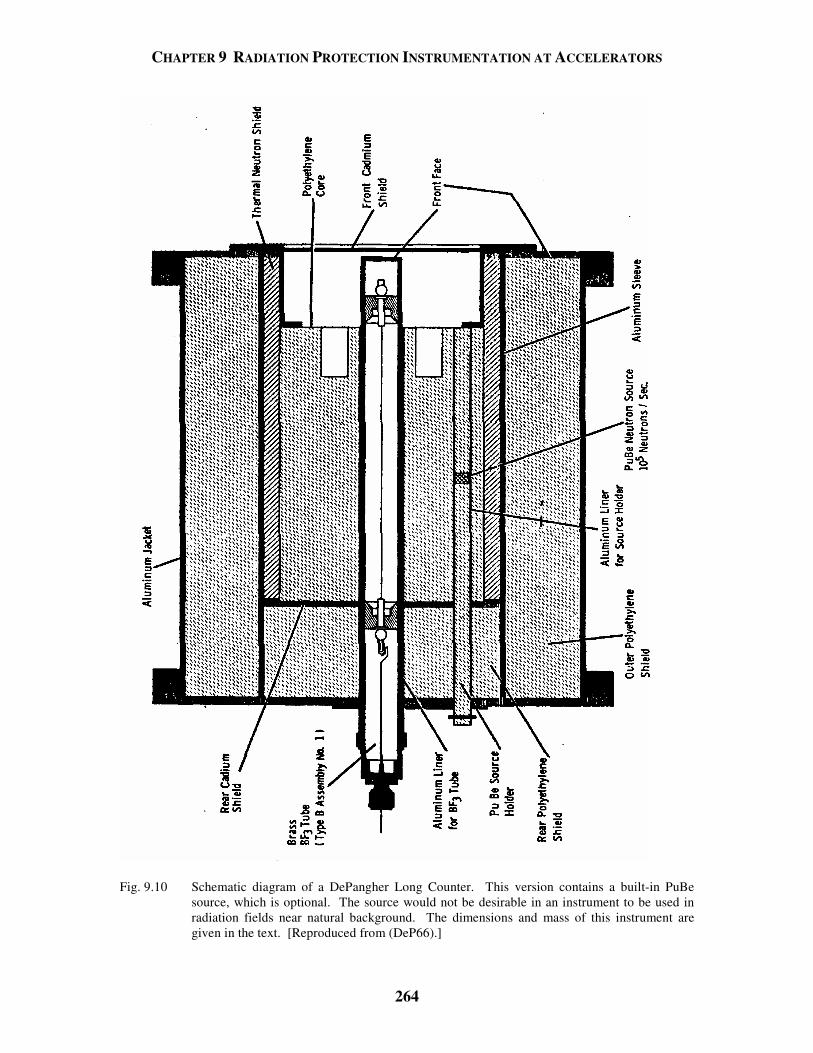
CHAPTER 9 RADIATION PROTECTION INSTRUMENTATION AT ACCELERATORS
264
Fig. 9.10 Schematic diagram of a DePangher Long Counter. This version contains a built-in PuBe
source, which is optional. The source would not be desirable in an instrument to be used in radiation fields near natural background. The dimensions and mass of this instrument are given in the text. [Reproduced from (DeP66).]
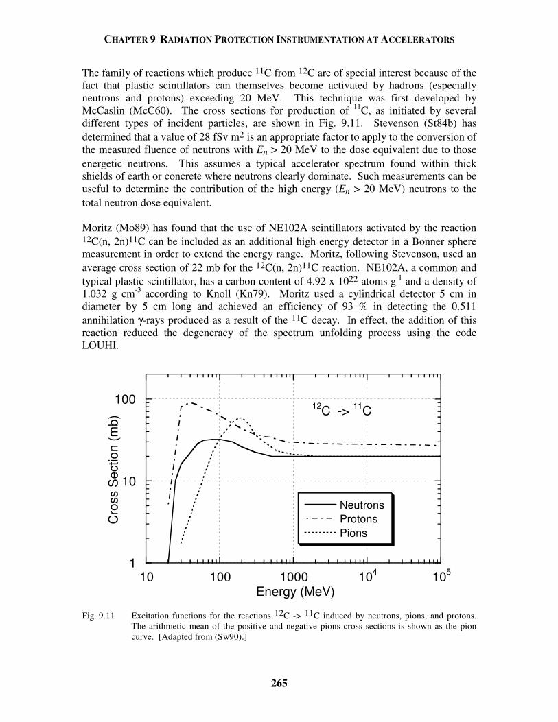
CHAPTER 9 RADIATION PROTECTION INSTRUMENTATION AT ACCELERATORS
265
The family of reactions which produce 11C from 12C are of special interest because of the fact that plastic scintillators can themselves become activated by hadrons (especially neutrons and protons) exceeding 20 MeV. This technique was first developed by McCaslin (McC60). The cross sections for production of 11C, as initiated by several different types of incident particles, are shown in Fig. 9.11. Stevenson (St84b) has determined that a value of 28 fSv m2 is an appropriate factor to apply to the conversion of the measured fluence of neutrons with En > 20 MeV to the dose equivalent due to those energetic neutrons. This assumes a typical accelerator spectrum found within thick shields of earth or concrete where neutrons clearly dominate. Such measurements can be useful to determine the contribution of the high energy (En > 20 MeV) neutrons to the total neutron dose equivalent. Moritz (Mo89) has found that the use of NE102A scintillators activated by the reaction 12C(n, 2n)11C can be included as an additional high energy detector in a Bonner sphere measurement in order to extend the energy range. Moritz, following Stevenson, used an average cross section of 22 mb for the 12C(n, 2n)11C reaction. NE102A, a common and typical plastic scintillator, has a carbon content of 4.92 x 10²² atoms g-1 and a density of 1.032 g cm-3 according to Knoll (Kn79). Moritz used a cylindrical detector 5 cm in diameter by 5 cm long and achieved an efficiency of 93 % in detecting the 0.511 annihilation γ-rays produced as a result of the 11C decay. In effect, the addition of this reaction reduced the degeneracy of the spectrum unfolding process using the code LOUHI.
1
10
100
10 100 1000 104 105
NeutronsProtonsPions
Cro
ss S
ectio
n (m
b)
Energy (MeV)
12C -> 11C
Fig. 9.11 Excitation functions for the reactions 12C -> 11C induced by neutrons, pions, and protons.
The arithmetic mean of the positive and negative pions cross sections is shown as the pion curve. [Adapted from (Sw90).]
CHAPTER 9 RADIATION PROTECTION INSTRUMENTATION AT ACCELERATORS
266
Figure 9.12 provides the excitation functions of some other useful reactions with very high thresholds. The Hg -> 149Tb reaction is a suitable monitor for very high energy particles and is commonly used as a beam calibrator. However, it has been found by Baker et al. (Ba84 and Ba91) that there are three reactions involving copper targets that are more useful for this purpose because they have longer half-lives than the 4.1 hr half- life of 149Tb. These cross sections have been measured for energies from 30 to 800 GeV and are included in Table 9.6.
10-1
100
101
102
103
100 101 102 103 104 105
Cro
ss S
ectio
n (m
b)
Neutron Energy (MeV)
12C ->7Be
198Hg ->149Tb
32S(n,p)32P
27Al(n,α)24Na
27Al ->22Na
Fig. 9.12 Excitation functions of several threshold reactions. [Adapted from (Th88).] 9.5.4 Fission Counters 233U, 235U, and 239Pu all have relatively large fission cross sections at low neutron energies. The Q-values are very large (approximately 200 MeV) so that huge output signals are possible. For higher energy "fast" neutrons, fission reactions become possible for other, lighter nuclei such as bismuth. The cross sections for fast neutrons of these reactions are shown in Fig. 9.13. Fission reactions have been exploited as neutron (or hadron) detectors at accelerators. The fission of 209Bi is especially interesting since this reaction has a threshold of about 50 MeV and also exhibits strong evidence that the neutron and proton-induced fission cross sections are approximately equal. Bismuth has been employed in ionization chambers where the large energy deposited by the fission fragments gives a clear "signature" of this process. Like the use of 11C, it can provide further information about high energy neutrons and resolve ambiguities in the unfolding of spectra from Bonner sphere data. McCaslin et.al. have summarized some interesting results obtained using this process (McC68).
CHAPTER 9 RADIATION PROTECTION INSTRUMENTATION AT ACCELERATORS
267
10-3
10-2
10-1
100
101
10-2 10-1 100 101 102 103 104 105
235U238UnatUnatBiFi
ssio
n C
ross
Sec
tion
(bar
ns)
Energy (MeV)
Fig. 9.13 Fission cross sections of some common target nuclides used in fission chambers for fast neutrons. The cross sections for fission of 235U are much larger at lower energies not shown. [Adapted partially from (Kn79) and from (Sw90).]
9.5.5 Proton Recoil Counters Knoll (Kn79) describes a variety of techniques for detecting neutrons based upon measuring the energy of recoil particles. The 3He(n, p)3H reaction has a reasonable cross section even into the MeV region but suffers from competition with (n, d) processes and elastic scattering. Elastic scattering of neutrons in which the energy of the recoil particle is measured and correlated with the neutron energy has received a great deal of attention. The most obvious recoil particle to measure is the proton because hydrogenous detector materials (e.g., plastic scintillator) are readily available and also because the proton can receive the most energy in the recoil process. Detector designers have been able to exploit the fact that scattering from hydrogen in the region En < 10 MeV is isotropic in the center of mass frame. Knoll has shown that the probability, P(Er), of creating a recoil proton having energy Er is also independent of angle in the laboratory frame within this energy domain (Kn79). Thus the recoil energy is only a function of the incident neutron energy. However, complexities enter the picture because in scintillators, carbon is present along with the hydrogen and can contribute recoil protons. Furthermore, the magnitude of the cross section is a function of neutron energy as is the efficiency of neutron detection in the scintillator. These effects, along with that of finite pulse height
CHAPTER 9 RADIATION PROTECTION INSTRUMENTATION AT ACCELERATORS
268
resolution, can lead to the need to resort to unfolding techniques in which the pulse height, indicative of the energy of the recoil proton, is correlated with the average neutron energy which could produce such a pulse. The technique has exhibited some promise in measuring the energy spectra of neutron radiation fields. A good summary is that of Griffith and Thorngate (Gr85) who were able to determine neutron energy spectra in the region between 2 and 20 MeV. 9.5.6 TEPCs and LET Spectrometry In mixed field dosimetry, a promising technique, now reaching commercial potential is that of the tissue-equivalent proportional chamber (TEPC) sometimes referred to as the "Rossi counter" after its inventor, H. Rossi (Ro55). The technique has been described by Brackenbush et al. (Br78). In this instrument tissue equivalent walls are employed to apply the Bragg-Gray principle. In such chambers, the pressure is maintained at low values, only a few torr (a few hundred pascals), so that the energy deposited is kept small. Thus, the energy so deposited will be equal to the linear energy transfer of the particle multiplied by the path length. At these low pressures, the gas-filled cavity has the same energy loss as does a sphere of tissue of diameter about 1 µm-hence an "equivalent diameter of 1 µm". In principle, determining the absorbed dose from events in such chambers is a straightforward unit conversion from a measured pulse height spectrum (calibrated in energy) to absorbed dose (in tissue) irrespective of the radiation field;
max
min
8(rad) 1.602 10 ( )i i
i i
CD iN i
Vρ−
=
== × , (9.28)
where the summation is over channels i (imin < i < imax , see below) corresponding to the radiation type of interest, V is the sensitive volume (cm3), ρ is the density (g cm-3), C converts the channel number to energy in MeV, and N (i) is the number of counts in channel number i. In such chambers, the transition between photon and neutron-induced events occurs at a pulse height of about 15 keV µm-1. It is possible to determine the quality factor, Q, from a single TEPC measurement. Under the conditions stated above, one can unfold from the pulse height spectrum the distribution of absorbed dose as a function of LET, D(L), using a formula derived by Rossi (Ro68). The formula is complicated by the fact that one must average over mean chord lengths in the chamber. Such a distribution is used to calculate quality factor, and hence the dose equivalent. The advent of microprocessors has made such instruments available as portable instruments. Fig. 9.14 shows a typical pulse height spectrum for such an instrument. In higher energy fields, dose distributions due to other particles with the same characteristic shapes but larger pulse sizes appear as the 2H, 3H, 3He, 4He and even 7Li "drop points". This obviously will add complexities to the unfolding procedures in the determination of LET spectra. A good discussion of the application of this technique is given by Vasilik et al. (Va85).
CHAPTER 9 RADIATION PROTECTION INSTRUMENTATION AT ACCELERATORS
269
101
102
103
104
105
106
107
0 20 40 60 80 100 120 140
Cou
nts/
Cha
nnel
or
Abs
orbe
d D
ose/
Cha
nnel
Channel Number
1.4 MeV Neutrons
60Co γ-rays
Start of neutron data
Event Distribution
Absorbed Dose Distribution Proton Drop
Point
Fig. 9.14 Pulse-height spectra from a tissue-equivalent proportional counter exposed to 1.4 MeV
neutrons and 60Co γ-rays. [Adapted from (Br78).] 9.5.7 The Recombination Chamber Technique An adaptation of the ion chamber that has shown considerable potential for usefulness as a dose equivalent meter in a mixed field of radiation is based on the exploitation of recombination phenomena in such chambers. As charged particles interact in such a chamber the gas is ionized. The electrodes will collect only those ions that do not recombine before they reach the cathode. The extent of such columnar recombination is dependent upon the average distance between the ions as well as upon the applied voltage. The biasing voltage sets the speed at which the ions migrate to the cathode. For a given voltage, a chamber should exhibit more severe recombination for the radiations having high LET (e.g., neutrons, heavy ions, etc.) than for those having low LET (electrons, photons, and muons). In the high LET situation, the slow moving positive ions are surrounded by a higher density of electrons than they would be in under conditions of low LET. Zielcyznski (Zi62) did the initial work on this topic. Baarli and Sullivan reported similar results over a somewhat larger range of values of quality factor Q (2 < Q < 20) and further refined the technique (Ba65). It turns out that the current, i (or charge if integrated over time), measured in a given radiation field, is related to the applied voltage V by the following approximate expression: i kV n= . (9.29)

CHAPTER 9 RADIATION PROTECTION INSTRUMENTATION AT ACCELERATORS
270
The power parameter, n, is approximately proportional to the quality factor Q and k is a constant proportional to the intensity of the radiation field. Cossairt et al. (Co84) have measured this effect using a mixed field of γ-rays and neutrons from a Pu-Be source. The results are shown in Fig. 9.15 over the range 1 < Q < 7. The relationship between Q and n determined in (Co84) for one particular chamber was fit linearly by n = 0.00762 + 0.016Q , (9.30a) or by using a power law,
95.0019.0 Qn = . (9.30b) Patterson and Thomas (Pa73) have reported similar results over a somewhat larger range of Q (2 < Q < 20). Typically, the response of such a chamber is measured as a function of applied voltage for the special chamber provided for the purpose over some voltage range, say, 20 < V < 1200 volts. In fields that are not steady with time, the response
Fig. 9.15 Response of a recombination chamber as a function of quality factor Q obtained in mixed
fields using radioactive sources. Two different fits to the data are presented [Reproduced from (Co84) and (Co85b).]
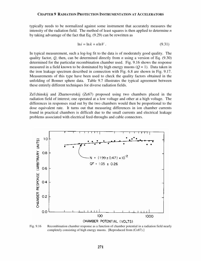
CHAPTER 9 RADIATION PROTECTION INSTRUMENTATION AT ACCELERATORS
271
typically needs to be normalized against some instrument that accurately measures the intensity of the radiation field. The method of least squares is then applied to determine n by taking advantage of the fact that Eq. (9.29) can be rewritten as ln ln lni k n V= + . (9.31) In typical measurement, such a log-log fit to the data is of moderately good quality. The quality factor, Q, then, can be determined directly from n using a version of Eq. (9.30) determined for the particular recombination chamber used. Fig. 9.16 shows the response measured in a field known to be dominated by high energy muons (Q = 1). Data taken in the iron leakage spectrum described in connection with Fig. 6.8 are shown in Fig. 9.17. Measurements of this type have been used to check the quality factors obtained in the unfolding of Bonner sphere data. Table 9.7 illustrates the typical agreement between these entirely different techniques for diverse radiation fields. Zel'chinskij and Zharnovetskij (Ze67) proposed using two chambers placed in the radiation field of interest; one operated at a low voltage and other at a high voltage. The differences in responses read out by the two chambers would then be proportional to the dose equivalent rate. It turns out that measuring differences in ion chamber currents found in practical chambers is difficult due to the small currents and electrical leakage problems associated with electrical feed-throughs and cable connectors.
Fig. 9.16 Recombination chamber response as a function of chamber potential in a radiation field nearly
completely consisting of high energy muons. [Reproduced from (Co87).]
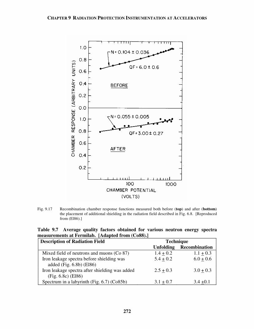
CHAPTER 9 RADIATION PROTECTION INSTRUMENTATION AT ACCELERATORS
272
Fig. 9.17 Recombination chamber response functions measured both before (top) and after (bottom) the placement of additional shielding in the radiation field described in Fig. 6.8. [Reproduced from (El86).]
Table 9.7 Average quality factors obtained for various neutron energy spectra measurements at Fermilab. [Adapted from (Co88).]
Description of Radiation Field Technique Unfolding Recombination Mixed field of neutrons and muons (Co 87) 1.4 + 0.2 1.1 + 0.3 Iron leakage spectra before shielding was
added (Fig. 6.8b) (El86) 5.4 + 0.2 6.0 + 0.6
Iron leakage spectra after shielding was added (Fig. 6.8c) (El86)
2.5 + 0.3 3.0 + 0.3
Spectrum in a labyrinth (Fig. 6.7) (Co85b) 3.1 + 0.7 3.4 +0.1
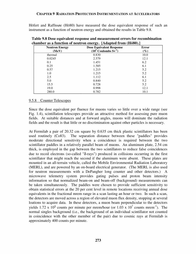
CHAPTER 9 RADIATION PROTECTION INSTRUMENTATION AT ACCELERATORS
273
Höfert and Raffnsøe (Hö80) have measured the dose equivalent response of such an instrument as a function of neutron energy and obtained the results in Table 9.8.
Table 9.8 Dose equivalent response and measurement errors for recombination chamber as a function of neutron energy. [Adapted from (Hö80).]
Neutron Energy (MeV)
Dose Equivalent Response (105 Coulombs Sv-1)
Error (%)
thermal 0.830 10.0 0.0245 2.579 12.1 0.1 1.451 6.2 0.25 1.585 6.1 0.57 1.215 5.2 1.0 1.215 5.2 2.5 1.112 6.1 5.0 0.840 5.2 15.5 0.728 5.2 19.0 0.998 12.1 280.0 0.782 10.1
9.5.8 Counter Telescopes Since the dose equivalent per fluence for muons varies so little over a wide range (see Fig. 1.4), scintillation telescopes provide an attractive method for assessing pure muon fields. At suitable distances and at forward angles, muons will dominate the radiation fields and the result is that little or no discrimination against other particles is necessary. At Fermilab a pair of 20.32 cm square by 0.635 cm thick plastic scintillators has been used routinely (Co83). The separation distance between these "paddles" provides moderate directional sensitivity when a coincidence is required between the two scintillator paddles in a relatively parallel beam of muons. An aluminum plate, 2.54 cm thick, is employed in the gap between the two scintillators to reduce false coincidences due to recoil electrons (so-called "δ-rays") produced in collisions occurring in the first scintillator that might reach the second if the aluminum were absent. These plates are mounted in an all-terrain vehicle, called the Mobile Environmental Radiation Laboratory (MERL), and are powered by an on-board electrical generator. (The MERL is also used for neutron measurements with a DePangher long counter and other detectors.) A microwave telemetry system provides gating pulses and proton beam intensity information so that normalized beam-on and beam-off (background) measurements can be taken simultaneously. The paddles were chosen to provide sufficient sensitivity to obtain statistical errors at the 20 per cent level in remote locations receiving annual dose equivalents in the fractional mrem range in a scan lasting an hour or two. In such a scan, the detectors are moved across a region of elevated muon flux density, stopping at several loations to acquire data. In these detectors, a muon beam perpendicular to the detectors yields 1.72 x 10⁵ counts per minute per mrem/hour (or 1.03 x 10⁷ counts mrem-1). The normal singles background (i.e., the background of an individual scintillator not counted in coincidence with the other member of the pair) due to cosmic rays at Fermilab is approximately 400 counts per minute.
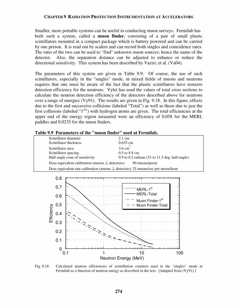
CHAPTER 9 RADIATION PROTECTION INSTRUMENTATION AT ACCELERATORS
274
Smaller, more portable systems can be useful in conducting muon surveys. Fermilab has built such a system, called a muon finder, consisting of a pair of small plastic scintillators mounted in a compact package which is battery powered and can be carried by one person. It is read out by scalers and can record both singles and coincidence rates. The ratio of the two can be used to "find" unknown muon sources; hence the name of the detector. Also, the separation distance can be adjusted to enhance or reduce the directional sensitivity. This system has been described by Vaziri, et al. (Va04). The parameters of this system are given in Table 9.9. Of course, the use of such scintillators, especially in the "singles" mode, in mixed fields of muons and neutrons requires that one must be aware of the fact that the plastic scintillators have nonzero detection efficiency for the neutrons. Vylet has used the values of total cross sections to calculate the neutron detection efficiency of the detectors described above for neutrons over a range of energies (Vy91). The results are given in Fig. 9.18. In this figure, effects due to the first and successive collisions (labeled “Total”) as well as those due to just the first collisions (labeled “1st”) with hydrogen atoms are given. The total efficiencies at the upper end of the energy region measured were an efficiency of 0.058 for the MERL paddles and 0.0235 for the muon finders. Table 9.9 Parameters of the "muon finder" used at Fermilab. Scintillator diameter 2.1 cm Scintillator thickness 0.635 cm Scintillator area 3.6 cm
2
Scintillator spacing 0.5 to 8.9 cm Half-angle cone of sensitivity 0.9 to 0.2 radians (51 to 11.5 deg. half-angle) Dose equivalent calibration (muons ⊥ detectors) 90 muons/µrem Dose equivalent rate calibration (muons ⊥ detectors) 25 muons/sec per mrem/hour
0
0.1
0.2
0.3
0.4
0.5
0.6
0.7
0.8
0.1 1 10 100
MERL-1st
MERL-Total
Muon Finder-1st
Muon Finder-Total
Effi
cien
cy
Neutron Energy (MeV) Fig. 9.18 Calculated neutron efficiencies of scintillation counters used in the "singles" mode at
Fermilab as a function of neutron energy as described in the text. [Adapted from (Vy91).]
CHAPTER 9 RADIATION PROTECTION INSTRUMENTATION AT ACCELERATORS
275
Problems 1. A cylindrical ion chamber is 5 cm in radius and 20 cm long. It is filled with
methane (CH4) at 1 one atmosphere absolute pressure. It is bombarded by a uniform flux density of high energy (minimum-ionizing) muons incident perpendicularly to one of the ends. One can safely make the assumption that the passage of the muons through the entire length of the chamber represents insignificant degradation of the muon energy or direction. The dose equivalent rate in the radiation field is 0.1 mrem hour-1.
a) Calculate the electric current that will be drawn from this chamber that represents the "signal" to be measured and correlated with the dose equivalent rate. One could use Table 1.2 to obtain values of (dE/dx)min and to obtain the density of CH4.
b) If the charge liberated in the chamber is collected (i.e., integrated electronically)
for 1 second and the chamber and circuit represent a capacitance of 10-10 Farads, calculate the size of the signal pulse in volts if one neglects any "pulse-shaping" of the readout electronics.
2. Consider the detector based on the 25.4 cm moderating sphere for which the corresponding response curve is displayed in Fig. 9.8.
a) Calculate the approximate absolute intrinsic detection efficiency for neutrons. This is to be done for the 2 < En < 8 MeV energy domain and the sharp peaks in the detector response curve are to be ignored (i.e., averaged out). In this problem, 100 % efficiency is defined to be 1 count generated for every neutron that strikes the sphere. Assume the incident neutrons to be aimed at the detector originating from a "point" source" despite the fact that this is not quite true.
b) Since the LiI detector only responds to thermal neutrons, calculate the efficiency
with which the moderator transforms fast neutrons incident upon it into thermal neutrons present at the LiI. For this calculation, neglect any "dopants" in the LiI, assume that the Li is "natural" lithium with respect to isotopic abundance and use the fact that the atomic weight of iodine is 127. The density of LiI is 3.5 g cm-3. Assume that the detector is 100% efficient in detecting thermal neutron captures within its volume.
CHAPTER 9 RADIATION PROTECTION INSTRUMENTATION AT ACCELERATORS
276
3. A BF3 proportional chamber is used in a DePangher long counter. This detector, when placed in a certain neutron field that is known to be dominated by neutrons of approximately 5 MeV kinetic energy, has a response due to neutrons of 1 count/minute. The detector sensitivity is that discussed in the text. The counter operates at one atmosphere absolute pressure, the atomic weight of boron is 10.8 while the atomic weight of fluorine is 19. At STP the density of BF3 is 2.99 grams liter-1.
a) What is the dose equivalent rate of this radiation field? b) If the radiation field persists full time, is this detector sufficiently sensitive to
detect a dose rate of 10 mrem year-1? c) In this radiation field, high energy minimum ionizing muons pass through this
detector, including the proportional counter. The largest muon signals in the proportional counter will obviously result when the muons pass lengthwise through the tube. If the tube is 40 cm long, what will be the size of the largest muon-induced signal relative to the neutron-induced signal? Is it likely that a simple discriminator circuit can be used to eliminate the muon-induced signals? It is quite permissible to estimate the value of (dE/dx)min by roughly interpolating among the values tabulated in Table 1.2.
4. One needs to understand the sensitivity of the technique of using the nuclear reaction 12C(n, 2n)11C in plastic scintillator to measure dose equivalent rate external to thick concrete or earth shielding near a high energy accelerator. The detector discussed in the text used by Moritz has a sensitive volume of approximately 100 cm3 (a 5 cm diameter by 5 cm long cylinder). The NE102A scintillator, from Knoll (Kn79), has a density of 1.032 g cm-3. This detector is nearly 100 % efficient at sensing the 0.511 MeV annihilation photons produced in the course of the 11C decay.
a) This detector is irradiated in a particular radiation field external to such
accelerator shielding. The irradiation, which is steady in time, is of sufficient length in time to result in saturation of the production of 11C in the scintillator. After the beam is turned off, the detector counts at a rate of 10 counts per minute (including appropriate decay-correction to the instant of beam shutdown). Calculate the flux density of neutrons with En > 20 MeV during the irradiation and use the result along with Stevenson's conclusion concerning the conversion from the flux density of neutrons with En > 20 MeV to dose equivalent to determine the dose equivalent rate.
b) Assuming this count rate is the smallest that can be reliably detected, how much
smaller in volume can the detector be for it to barely be sensitive to a dose equivalent rate of 2 mrem hour-1?
APPENDIX A SUMMARY DESCRIPTIONS OF COMMONLY USED MONTE CARLO CODES
277
This appendix provides brief summary descriptions of some of the more prominent Monte Carlo codes used at modern particle accelerators. The reader should be cautioned that most of these codes are being constantly improved and updated. The wisest practice in using them is to consult with the authors of the codes directly who can provide detailed, current in formation. CASIM A. Van Ginneken developed this “Cascade Simulation” program (Va75). It was designed to simulate the average behavior of hadrons in the region 10 to 1000 GeV and has been extended to 20 TeV (Va87). It uses inclusive production distributions directly in order to obtain the particles to follow. The particle production algorithm is based upon the Hagedorn-Ranft thermodynamic model. Only one or two high energy particles are created in each collision and these carry a weight related to the probability of their production and the energy carried with them. Path length stretching and particle splitting have been introduced. Electromagnetic showers resulting from πo production are calculated using the companion code AEGIS. Simple "standardized" geometries are available. However, the user generally writes a FORTRAN subroutine to set up the geometry of interest. This subroutine consists of "logical" (i.e., "IF", etc.) statements used to deduce the material or magnetic field in which a particle being tracked is found at a given "time" in the calculation from the particle's spatial and directional coordinates. The program readily allows magnetic fields to be used. A muon version called CASIMU (now MUSIM) has been written (Va87). The accuracy of the hadron version has been verified for energies up to 800 GeV (Co82a and Co85a). The muon version has also been verified for energies up to 800 GeV for production and transport of muons in real-life, complicated shields (Co89a and Co89b). Normally, CASIM is not set up to follow particles with momenta less than 300 MeV/c, which corresponds to a kinetic energy of 47 MeV for nucleons. All low energy phenomena, then, is obtained by matching energy spectra and fluence at this energy with results of codes capable of tracking lower energy particles (e.g., HETC, FLUKA, and MARS). At Fermilab, CASIM has been replaced by MARS as the code of choice. Results obtained using CASIM continue to serve as useful benchmarks. EGS EGS, the “Electron Gamma Shower” code is a powerful code for calculating electromagnetic cascades. A recent version is EGS4. A complete description of this code system has been written by Nelson et al. (Ne85, Ne90). This program provides a Monte Carlo analysis of electron and photon scattering including shower generation. In its standard usage, it does not calculate hadron or muon production directly. The lower limit of its validity is about 10 keV while the upper limit of its validity is at least 1 TeV. Possible target materials span the periodic table. As the electron encounters target atoms, it is scattered randomly to mimic the known mechanisms of electron scattering. When secondary particles arise, they are loaded into a stack from which EGS4 selects sequentially the lowest energy particle and then traces out its further path until it leaves the target or until its energy falls below a selected cut-off value. The final kinematical
APPENDIX A SUMMARY DESCRIPTIONS OF COMMONLY USED MONTE CARLO CODES
278
and charge properties of all the particles are noted and summed for all particles in the shower concluding with a "history" of all of them. Improvements with the code are continuously being made. The code is a fundamental tool at many laboratories that have electron accelerators. The code has been found to be extremely useful in applications in medicine and also in modeling the performance of high energy physics apparatus. The EGS code system is available from the Stanford Linear Accelerator Center. FLUKA FLUKA is an integrated, versatile multi-particle Monte Carlo program, capable of handling a wide variety of radiation transport problems. Its energy range extends from one keV (for neutrons, thermal energies) to thousands of TeV. FLUKA can simulate with a similar level of accuracy the propagation of hadronic and electromagnetic cascades, cosmic muons, slowing-down neutrons and synchrotron radiation in the keV region. An original treatment of multiple Coulomb scattering allows the code to handle accurately some challenging problems such as electron backscattering and energy deposition in thin layers. In a fully analog mode, FLUKA can be used in detector studies to predict fluctuations, coincidences and anti-coincidences. On the other hand, a rich supply of biasing options makes it well suited for studies of rare events, deep penetration and shielding in general. This code originated as high-energy particle transport code developed by a CERN-Helsinki-Leipzig collaboration, principally by J. Ranft as discussed by Aarnio et al. (Aa86). More recently, it has been completely rewritten and extended to low energies as discussed by Fassò et al. (Fa93). It handles more than 30 different particles, including neutrons from thermal energies to about 20 TeV and photons from 1 keV to thousands of TeV. Several biasing techniques are available. Recoil protons and protons from N(n,p) reactions are transported explicitly. This code is currently available from the Stanford Linear Accelerator Center. HETC and LAHET This code, developed over many years under the leadership of R. G. Alsmiller at the Oak Ridge National Laboratory, is considered by some to be the benchmark hadron shielding code of choice. It has been upgraded many times and can, in suitably augmented versions, follow particles from the 20 TeV region down to thermal energies. It is an extremely flexible code but has the important disadvantage that the individual events are written to mass storage. It is the responsibility of the user to write a program to analyze the results. In terms of CPU-time HETC is also relatively slow so that calculations to be done should be carefully selected. It is seen to be preferable to use selected HETC runs to calibrate other faster, but less accurate codes. It has been described by Armstrong (Ar80) and Gabriel (Ga85). It now uses the same event generator used for FLUKA. A modified version of this code, developed at the Los Alamos National Laboratory (LANL) as LAHET, has been described by Prael and Lichtenstein (Pr89). It is available from the Los Alamos National Laboratory. This variant permits the transport of neutrons, photons, and light nuclei up to 4He and employs the geometric capabilities of the MCNP code.
APPENDIX A SUMMARY DESCRIPTIONS OF COMMONLY USED MONTE CARLO CODES
279
MARS The MARS Monte Carlo code system has been under continuous development over a number of years by N. Mokhov et al. (Ka89, Mo95, Kr97, Mo04). Early results were compared by Mokhov and Cossairt (Mo86) with those obtained using then-current versions of CASIM and FLUKA with good agreement. The code allows exclusive and fast inclusive simulation of three-dimensional hadronic and electromagnetic cascades for shielding, accelerator, and detector components in the energy range from a fraction of an electron volt up to 100 TeV. The current version, MARS15, uses the phenomenological model for inclusive hadron- and photon-nucleus interactions for E > 5 GeV, exclusive cascade-exciton model at 1 MeV < E < 5 GeV, and, by using the LAQGSM event generator, full theoetically consistent modeling of exclusive distributions of secondary particles, spallation, fission, and fragmentation products for hadron and heavy-ion beams of any energy. MARS15 includes photo- and electro-production of hadrons and muons, advanced algorithms for the 3-body decays, precise particle tracking in magnetic fields, synchrotron radiation by electrons and muons, extended histogramming capabilities and improved material description and computational performance. Along with direct energy deposition calculations, a set of dose conversion per fluence factors for all particles including neutrinos is incorporated. The code includes links to the MCNP4C code for neutron and photon transport below 20 MeV, to the ANSYS code for thermal and stress analyses, and to the MAD and STRUCT codes for lattice description for multi-turn particle tracking in large synchrotrons and collider rings. The geometry module allows the use of a set of the pre-defined shapes, arbitrary user-defined 3-D descriptions, the object-oriented engine coupled with VRML/2.0 (an approved standard web-oriented three dimensional geometry description), or direct use of MCNP and FLUKA geometry input desks. The code is provided with a user-friendly graphical-use interface for geometry and calculated results visualization and debugging. A parallelized version of the code can run in a multi-processor mode. The developments were induced by numerous challenging applications - Fermilab accelerator, detector and shielding upgrades, Large Hadron Collider machine and detector studies, muon and electron-positron colliders etc - as well as by a continuous desire to increase code reliability, flexibility and user friendliness. This code is continously updated and improved and is can be obtained from Fermilab. It is likely the most advanced high energy code available. MCNP MCNP is a general-purpose Monte Carlo N-particle code that can be used for neutron, photon, electron, or coupled neutron/photon/electron transport, including the capability to handle situations involving nuclear criticality. This code has been developed at the Los Alamos National Laboratory and is well documented in LANL reports (e.g., Br97). The code treats an arbitrary three-dimensional configuration of materials in geometric cells bounded by first- and second-degree surfaces and fourth-degree elliptical tori. The neutron energy regime is from 10-11 MeV to 150 MeV, and the photon and electron energy regimes are from 1 keV to 1000 MeV. For neutrons, all reactions given in a particular cross-section evaluation (such as ENDF/B-VI cross section database) are accounted for. Thermal neutrons are described by both the free gas and thermal particle
APPENDIX A SUMMARY DESCRIPTIONS OF COMMONLY USED MONTE CARLO CODES
280
scattering models. For photons, the code takes account of incoherent and coherent scattering, the possibility of fluorescent emission after photoelectric absorption, absorption in pair production with local emission of annihilation radiation, and bremsstrahlung. A continuous slowing down model is used for electron transport that includes positrons, x-rays, and bremsstrahlung but does not include external or self-induced fields. Important standard features that make MCNP very versatile and easy to use include a powerful general source, criticality source, and surface source; both geometry and output tally plotters; a rich collection of variance reduction techniques; a flexible tally structure (including a pulse-height tally); and an extensive collection of cross-section data. The current version is available from the Los Alamos National Laboratory.
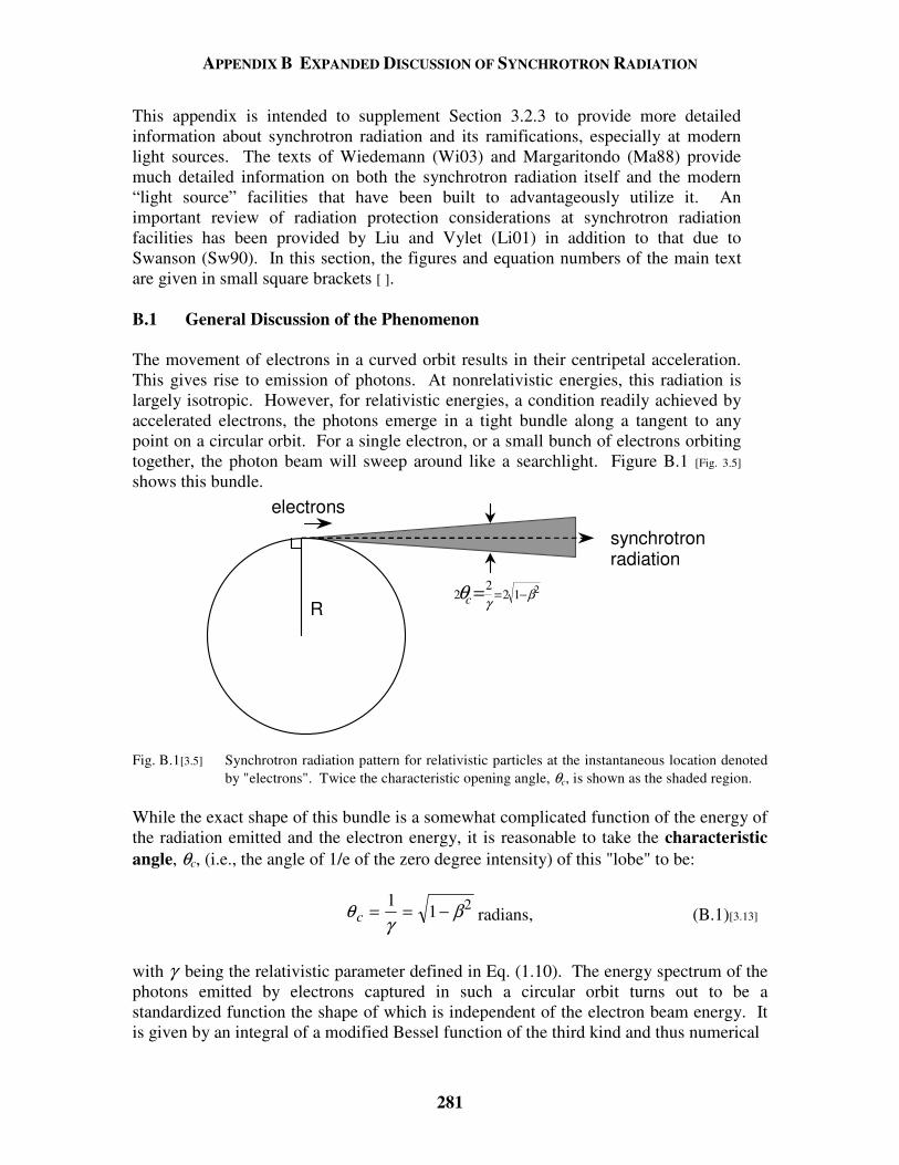
APPENDIX B EXPANDED DISCUSSION OF SYNCHROTRON RADIATION
281
This appendix is intended to supplement Section 3.2.3 to provide more detailed information about synchrotron radiation and its ramifications, especially at modern light sources. The texts of Wiedemann (Wi03) and Margaritondo (Ma88) provide much detailed information on both the synchrotron radiation itself and the modern “light source” facilities that have been built to advantageously utilize it. An important review of radiation protection considerations at synchrotron radiation facilities has been provided by Liu and Vylet (Li01) in addition to that due to Swanson (Sw90). In this section, the figures and equation numbers of the main text are given in small square brackets [ ]. B.1 General Discussion of the Phenomenon The movement of electrons in a curved orbit results in their centripetal acceleration. This gives rise to emission of photons. At nonrelativistic energies, this radiation is largely isotropic. However, for relativistic energies, a condition readily achieved by accelerated electrons, the photons emerge in a tight bundle along a tangent to any point on a circular orbit. For a single electron, or a small bunch of electrons orbiting together, the photon beam will sweep around like a searchlight. Figure B.1 [Fig. 3.5] shows this bundle.
R
electrons
22
2 1 2θγ
βc = = −
synchrotronradiation
Fig. B.1[3.5] Synchrotron radiation pattern for relativistic particles at the instantaneous location denoted
by "electrons". Twice the characteristic opening angle, θc, is shown as the shaded region. While the exact shape of this bundle is a somewhat complicated function of the energy of the radiation emitted and the electron energy, it is reasonable to take the characteristic angle, θc, (i.e., the angle of 1/e of the zero degree intensity) of this "lobe" to be:
θγ
βc = = −11 2
radians, (B.1)[3.13]
with γ being the relativistic parameter defined in Eq. (1.10). The energy spectrum of the photons emitted by electrons captured in such a circular orbit turns out to be a standardized function the shape of which is independent of the electron beam energy. It is given by an integral of a modified Bessel function of the third kind and thus numerical
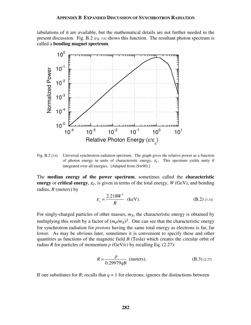
APPENDIX B EXPANDED DISCUSSION OF SYNCHROTRON RADIATION
282
tabulations of it are available, but the mathematical details are not further needed in the present discussion. Fig. B.2 [Fig. 3.6] shows this function. The resultant photon spectrum is called a bending magnet spectrum.
10-5
10-4
10-3
10-2
10-1
100
10-4 10-3 10-2 10-1 100 101
Nor
mal
ized
Pow
er
Relative Photon Energy (ε/εc)
Fig. B.2 [3.6] Universal synchrotron radiation spectrum. The graph gives the relative power as a function
of photon energy in units of characteristic energy, εc. This spectrum yields unity if integrated over all energies. [Adapted from (Sw90).]
The median energy of the power spectrum, sometimes called the characteristic energy or critical energy, εc, is given in terms of the total energy, W (GeV), and bending radius, R (meters) by
32.218c
WR
ε = (keV). (B.2) [3.14]
For singly-charged particles of other masses, mx, the characteristic energy is obtained by multiplying this result by a factor of (me/mx)3. One can see that the characteristic energy for synchrotron radiation for protons having the same total energy as electrons is far, far lower. As may be obvious later, sometimes it is convenient to specify these and other quantities as functions of the magnetic field B (Tesla) which creates the circular orbit of radius R for particles of momentum p (GeV/c) by recalling Eq. (2.27):
0.29979p
RqB
= (meters). (B.3) [2.27]
If one substitutes for R; recalls that q = 1 for electrons; ignores the distinctions between
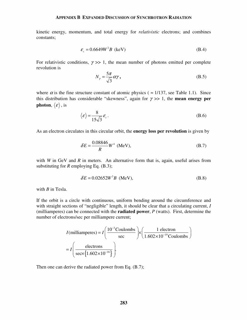
APPENDIX B EXPANDED DISCUSSION OF SYNCHROTRON RADIATION
283
kinetic energy, momentum, and total energy for relativistic electrons; and combines constants;
20.6649c W Bε = (keV) (B.4) For relativistic conditions, γ >> 1, the mean number of photons emitted per complete revolution is
53
Nγπ αγ= , (B.5)
where α is the fine structure constant of atomic physics ( ≈ 1/137, see Table 1.1). Since this distribution has considerable “skewness”, again for γ >> 1, the mean energy per photon, ε , is
8
15 3 cε ε= . (B.6)
As an electron circulates in this circular orbit, the energy loss per revolution is given by
40.08846E W
Rδ = (MeV), (B.7)
with W in GeV and R in meters. An alternative form that is, again, useful arises from substituting for R employing Eq. (B.3); 30.02652E W Bδ = (MeV), (B.8) with B in Tesla. If the orbit is a circle with continuous, uniform bending around the circumference and with straight sections of “negligible” length, it should be clear that a circulating current, I (milliamperes) can be connected with the radiated power, P (watts). First, determine the number of electrons/sec per milliampere current;
3
19
16
10 Coulombs 1 electron(milliamperes)
sec 1.602 10 Coulombs
electrons.
sec 1.602 10
I I
I
−
−
−
= × ×
= × ×
Then one can derive the radiated power from Eq. (B.7);
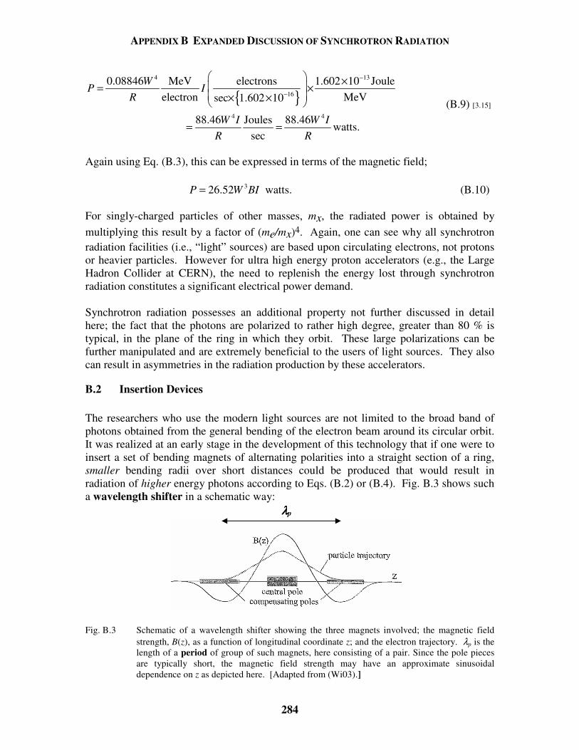
APPENDIX B EXPANDED DISCUSSION OF SYNCHROTRON RADIATION
284
4 13
16
4 4
0.08846 MeV electrons 1.602 10 Jouleelectron MeVsec 1.602 10
88.46 Joules 88.46watts.
sec
WP I
R
W I W IR R
−
−
× = × × ×
= =
(B.9) [3.15]
Again using Eq. (B.3), this can be expressed in terms of the magnetic field;
326.52P W BI= watts. (B.10)
For singly-charged particles of other masses, mx, the radiated power is obtained by multiplying this result by a factor of (me/mx)4. Again, one can see why all synchrotron radiation facilities (i.e., “light” sources) are based upon circulating electrons, not protons or heavier particles. However for ultra high energy proton accelerators (e.g., the Large Hadron Collider at CERN), the need to replenish the energy lost through synchrotron radiation constitutes a significant electrical power demand. Synchrotron radiation possesses an additional property not further discussed in detail here; the fact that the photons are polarized to rather high degree, greater than 80 % is typical, in the plane of the ring in which they orbit. These large polarizations can be further manipulated and are extremely beneficial to the users of light sources. They also can result in asymmetries in the radiation production by these accelerators.
B.2 Insertion Devices The researchers who use the modern light sources are not limited to the broad band of photons obtained from the general bending of the electron beam around its circular orbit. It was realized at an early stage in the development of this technology that if one were to insert a set of bending magnets of alternating polarities into a straight section of a ring, smaller bending radii over short distances could be produced that would result in radiation of higher energy photons according to Eqs. (B.2) or (B.4). Fig. B.3 shows such a wavelength shifter in a schematic way:
λλλλp
Fig. B.3 Schematic of a wavelength shifter showing the three magnets involved; the magnetic field strength, B(z), as a function of longitudinal coordinate z; and the electron trajectory. λp is the length of a period of group of such magnets, here consisting of a pair. Since the pole pieces are typically short, the magnetic field strength may have an approximate sinusoidal dependence on z as depicted here. [Adapted from (Wi03).]
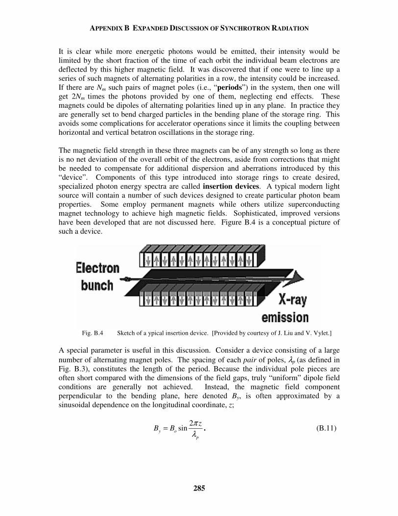
APPENDIX B EXPANDED DISCUSSION OF SYNCHROTRON RADIATION
285
It is clear while more energetic photons would be emitted, their intensity would be limited by the short fraction of the time of each orbit the individual beam electrons are deflected by this higher magnetic field. It was discovered that if one were to line up a series of such magnets of alternating polarities in a row, the intensity could be increased. If there are Nm such pairs of magnet poles (i.e., “periods”) in the system, then one will get 2Nm times the photons provided by one of them, neglecting end effects. These magnets could be dipoles of alternating polarities lined up in any plane. In practice they are generally set to bend charged particles in the bending plane of the storage ring. This avoids some complications for accelerator operations since it limits the coupling between horizontal and vertical betatron oscillations in the storage ring. The magnetic field strength in these three magnets can be of any strength so long as there is no net deviation of the overall orbit of the electrons, aside from corrections that might be needed to compensate for additional dispersion and aberrations introduced by this “device”. Components of this type introduced into storage rings to create desired, specialized photon energy spectra are called insertion devices. A typical modern light source will contain a number of such devices designed to create particular photon beam properties. Some employ permanent magnets while others utilize superconducting magnet technology to achieve high magnetic fields. Sophisticated, improved versions have been developed that are not discussed here. Figure B.4 is a conceptual picture of such a device.
Fig. B.4 Sketch of a ypical insertion device. [Provided by courtesy of J. Liu and V. Vylet.]
A special parameter is useful in this discussion. Consider a device consisting of a large number of alternating magnet poles. The spacing of each pair of poles, λp (as defined in Fig. B.3), constitutes the length of the period. Because the individual pole pieces are often short compared with the dimensions of the field gaps, truly “uniform” dipole field conditions are generally not achieved. Instead, the magnetic field component perpendicular to the bending plane, here denoted By, is often approximated by a sinusoidal dependence on the longitudinal coordinate, z;
2siny o
p
zB B
πλ
= . (B.11)
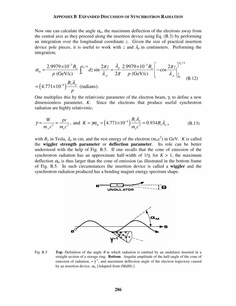
APPENDIX B EXPANDED DISCUSSION OF SYNCHROTRON RADIATION
286
Now one can calculate the angle αm, the maximum deflection of the electrons away from the central axis as they proceed along the insertion device using Eq. (B.3) by performing an integration over the longitudinal coordinate z. Given the size of practical insertion device pole pieces, it is useful to work with z and λp in centimeters. Performing the integration;
( )
/ 43 3/ 4
0
4
2.9979 10 2.9979 102 2sin cos
(GeV/c) 2 (GeV/c)
4.771 10 (radians).
p
p po om o
p p
o p
B Bz zdz
p p
B
p
λλ λπ πα
λ π λ
λ
− −
−
× ×= = −
= ×
(B.12)
One multiplies this by the relativistic parameter of the electron beam, γ, to define a new dimensionless parameter, K. Since the electrons that produce useful synchrotron radiation are highly relativistic;
( )42 2 2, and 4.771 10 0.934o p
m o po o o
BW pcK B
m c m c m c
λγ γα λ−= ≈ = = × = , (B.13)
with Bo in Tesla, λp in cm, and the rest energy of the electron (moc2) in GeV. K is called the wiggler strength parameter or deflection parameter. Its role can be better understood with the help of Fig. B.5. If one recalls that the cone of emission of the synchrotron radiation has an approximate half-width of 1/γ, for K > 1, the maximum deflection αm is thus larger than the cone of emission (as illustrated in the bottom frame of Fig. B.5. In such circumstances the insertion device is called a wiggler and the synchrotron radiation produced has a bending magnet energy spectrum shape.
Fig. B.5 Top: Definition of the angle θ at which radiation is emitted by an undulator inserted in a straight section of a storage ring. Bottom: Angular amplitude of the half-angle of the cone of emission of radiation, ≈ γ−1, and maximum deflection angle of the electron trajectory caused by an insertion device, αm. [Adapted from (Ma88).]
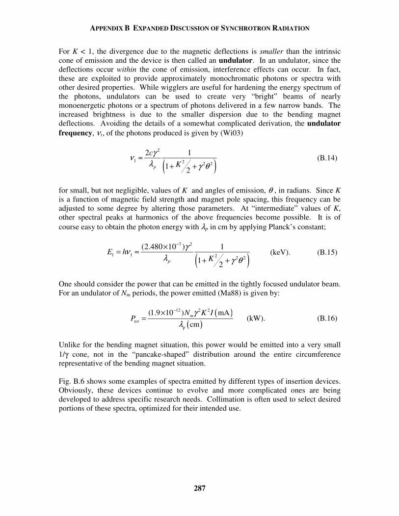
APPENDIX B EXPANDED DISCUSSION OF SYNCHROTRON RADIATION
287
For K < 1, the divergence due to the magnetic deflections is smaller than the intrinsic cone of emission and the device is then called an undulator. In an undulator, since the deflections occur within the cone of emission, interference effects can occur. In fact, these are exploited to provide approximately monochromatic photons or spectra with other desired properties. While wigglers are useful for hardening the energy spectrum of the photons, undulators can be used to create very “bright” beams of nearly monoenergetic photons or a spectrum of photons delivered in a few narrow bands. The increased brightness is due to the smaller dispersion due to the bending magnet deflections. Avoiding the details of a somewhat complicated derivation, the undulator frequency, ν1, of the photons produced is given by (Wi03)
( )2
1 2 2 2
2 1
1 2p
cK
γνλ γ θ
≈+ +
(B.14)
for small, but not negligible, values of K and angles of emission, θ , in radians. Since K is a function of magnetic field strength and magnet pole spacing, this frequency can be adjusted to some degree by altering those parameters. At “intermediate” values of K, other spectral peaks at harmonics of the above frequencies become possible. It is of course easy to obtain the photon energy with λp in cm by applying Planck’s constant;
( )7 2
1 1 2 2 2
(2.480 10 ) 1
1 2p
E hK
γνλ γ θ
−×= ≈+ +
(keV). (B.15)
One should consider the power that can be emitted in the tightly focused undulator beam. For an undulator of Nm periods, the power emitted (Ma88) is given by:
( )( )
12 2 2
p
(1.9 10 ) mAcmm
tot
N K IP
γλ
−×= (kW). (B.16)
Unlike for the bending magnet situation, this power would be emitted into a very small 1/γ cone, not in the “pancake-shaped” distribution around the entire circumference representative of the bending magnet situation. Fig. B.6 shows some examples of spectra emitted by different types of insertion devices. Obviously, these devices continue to evolve and more complicated ones are being developed to address specific research needs. Collimation is often used to select desired portions of these spectra, optimized for their intended use.
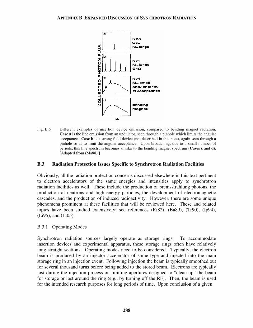
APPENDIX B EXPANDED DISCUSSION OF SYNCHROTRON RADIATION
288
Fig. B.6 Different examples of insertion device emission, compared to bending magnet radiation. Case a is the line emission from an undulator, seen through a pinhole which limits the angular acceptance. Case b is a strong field device (not described in this note), again seen through a pinhole so as to limit the angular acceptance. Upon broadening, due to a small number of periods, this line spectrum becomes similar to the bending magnet spectrum (Cases c and d). [Adapted from (Ma88).]
B.3 Radiation Protection Issues Specific to Synchrotron Radiation Facilities Obviously, all the radiation protection concerns discussed elsewhere in this text pertinent to electron accelerators of the same energies and intensities apply to synchrotron radiation facilities as well. These include the production of bremsstrahlung photons, the production of neutrons and high energy particles, the development of electromagnetic cascades, and the production of induced radioactivity. However, there are some unique phenomena prominent at these facilities that will be reviewed here. These and related topics have been studied extensively; see references (Ri82), (Ba89), (Tr90), (Ip94), (Li95), and (Li05). B.3.1 Operating Modes Synchrotron radiation sources largely operate as storage rings. To accommodate insertion devices and experimental apparatus, these storage rings often have relatively long straight sections. Operating modes need to be considered. Typically, the electron beam is produced by an injector accelerator of some type and injected into the main storage ring in an injection event. Following injection the beam is typically smoothed out for several thousand turns before being added to the stored beam. Electrons are typically lost during the injection process on limiting apertures designed to “clean-up” the beam for storage or lost around the ring (e.g., by turning off the RF). Then, the beam is used for the intended research purposes for long periods of time. Upon conclusion of a given
APPENDIX B EXPANDED DISCUSSION OF SYNCHROTRON RADIATION
289
period of storage ring operations (i.e, at the end of a “store”), the beam is generally disposed of in a beam absorber, and the cycle is repeated. A relatively recent advancement made to improve the quality of operations is the capability to replenish the beam by delivering electrons from the injector to the storage ring in a so-called top-off mode. Often the personnel protection requirements and beamline access restrictions imposed on the researchers are considerably different during injection events and storage ring operations due to the differences in the levels and types of radiological hazards presented. Typically, radiological problems are most prominent during the injection events because at that time, errors of beam tuning may result in point losses and the rate of beam delivery can be large and is intrinsically limited only by the output of the injector. Beam loss “accidents” may occur. Obviously this applies also to the top-off mode of operation. During pure storage ring operations, since accelerator orbits have been established to achieve a useful beam lifetime, inductive time constants render sudden, large losses due to mistuning or collapse of the magnetic field (e.g., during a power failure) much less probable. Point losses can, however, occur due to other types of events such as the sudden closure of vacuum valves or some other unintended movement of material into the beam. However, while the stored beam current may be significant, during the storage ring mode (i.e., not during injection or topping-off), the total number of stored electrons is limited, and may serve to apply an upper limit to the radiological consequences of beam loss events. At some facilities devices called beam stops, shutters, or injection stoppers are inserted into the front end of each beamline and used to protect personnel and equipment from the consequences of beam losses during injection events. Obviously it is imperative to fully understand the beam loss characteristics at every stage of operation. Fig. B.7 shows the layout of a portion of a typical synchrotron radiation facility showing the installation of some types of safety equipment used in various operational modes.
Fig. B.7 Typical synchrotron radiation facility experimental installation. The storage ring is at the
bottom of the frame. So called “ratchet-walls” separate the experimental installations from the main storage ring. [Adapted from (NC03).]
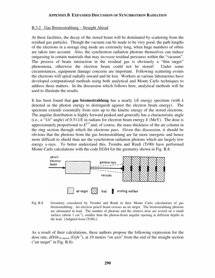
APPENDIX B EXPANDED DISCUSSION OF SYNCHROTRON RADIATION
290
B.3.2 Gas Bremsstrahlung – Straight Ahead At these facilities, the decay of the stored beam will be dominated by scattering from the residual gas particles. Though the vacuum can be made to be very good, the path lengths of the electrons in a storage ring mode are extremely long, when huge numbers of orbits are taken into account. Also, the synchrotron radiation photons themselves can induce outgassing in certain materials that may increase residual pressures within the “vacuum”. The process of beam interaction in the residual gas is obviously a “thin target” phenomena, otherwise the electron beam could not be stored! Under some circumstances, equipment damage concerns are important. Following scattering events the electrons will spiral radially inward and be lost. Workers at various laboratories have developed computational methods using both analytical and Monte Carlo techniques to address these matters. In the discussion which follows here, analytical methods will be used to illustrate the results. It has been found that gas bremsstrahlung has a nearly 1/k energy spectrum (with k denoted as the photon energy to distinguish against the electron beam energy). The spectrum extends essentially from zero up to the kinetic energy of the stored electrons. The angular distribution is highly forward peaked and generally has a characteristic angle (i.e., a “1/e” angle) of 0.511/E in radians for electron beam energy E (MeV). The dose is approximately proportional to E2.5 and, of course, the mass thickness of the air column in the ring section through which the electrons pass. Given this discussion, it should be obvious that the photons from the gas bremsstrahlung are far more energetic and hence more difficult to shield than are the synchrotron radiation photons which are largely low energy x-rays. To better understand this, Tromba and Rindi (Tr90) have performed Monte Carlo calculations with the code EGS4 for the geometry shown in Fig. B.8.
Fig. B.8 Geometry considered by Tromba and Rindi in their Monte Carlo calculations of gas
bremsstrahlung. An electron pencil beam crosses an air target. The bremsstrahlung photons are attenuated in lead. The number of photons and the relative dose are scored on a small surface (about 1 cm 2), smaller than the photon-beam angular opening at different depths in the lead. [Adapted from (Tr90).]
As a result of their calculations, these authors propose the following expression for the dose rate, dD/dt10 meters (Gyh-1), at 10 meters “on axis” from the end of the straight section (“air target” in Fig. B.8):
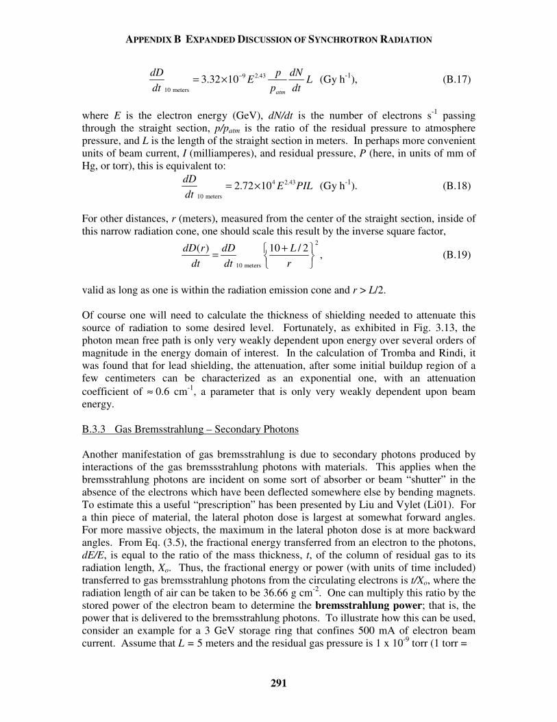
APPENDIX B EXPANDED DISCUSSION OF SYNCHROTRON RADIATION
291
9 2.43
10 meters3.32 10
atm
dD p dNE L
dt p dt−= × (Gy h-1), (B.17)
where E is the electron energy (GeV), dN/dt is the number of electrons s-1 passing through the straight section, p/patm is the ratio of the residual pressure to atmosphere pressure, and L is the length of the straight section in meters. In perhaps more convenient units of beam current, I (milliamperes), and residual pressure, P (here, in units of mm of Hg, or torr), this is equivalent to:
4 2.43
10 meters2.72 10
dDE PIL
dt= × (Gy h-1). (B.18)
For other distances, r (meters), measured from the center of the straight section, inside of this narrow radiation cone, one should scale this result by the inverse square factor,
2
10 meters
( ) 10 / 2dD r dD Ldt dt r
+ =
, (B.19)
valid as long as one is within the radiation emission cone and r > L/2. Of course one will need to calculate the thickness of shielding needed to attenuate this source of radiation to some desired level. Fortunately, as exhibited in Fig. 3.13, the photon mean free path is only very weakly dependent upon energy over several orders of magnitude in the energy domain of interest. In the calculation of Tromba and Rindi, it was found that for lead shielding, the attenuation, after some initial buildup region of a few centimeters can be characterized as an exponential one, with an attenuation coefficient of ≈ 0.6 cm-1, a parameter that is only very weakly dependent upon beam energy. B.3.3 Gas Bremsstrahlung – Secondary Photons Another manifestation of gas bremsstrahlung is due to secondary photons produced by interactions of the gas bremssstrahlung photons with materials. This applies when the bremsstrahlung photons are incident on some sort of absorber or beam “shutter” in the absence of the electrons which have been deflected somewhere else by bending magnets. To estimate this a useful “prescription” has been presented by Liu and Vylet (Li01). For a thin piece of material, the lateral photon dose is largest at somewhat forward angles. For more massive objects, the maximum in the lateral photon dose is at more backward angles. From Eq. (3.5), the fractional energy transferred from an electron to the photons, dE/E, is equal to the ratio of the mass thickness, t, of the column of residual gas to its radiation length, Xo. Thus, the fractional energy or power (with units of time included) transferred to gas bremsstrahlung photons from the circulating electrons is t/Xo, where the radiation length of air can be taken to be 36.66 g cm-2. One can multiply this ratio by the stored power of the electron beam to determine the bremsstrahlung power; that is, the power that is delivered to the bremsstrahlung photons. To illustrate how this can be used, consider an example for a 3 GeV storage ring that confines 500 mA of electron beam current. Assume that L = 5 meters and the residual gas pressure is 1 x 10⁻⁹ torr (1 torr =
APPENDIX B EXPANDED DISCUSSION OF SYNCHROTRON RADIATION
292
1 mm of Hg = 1/760 of an atmosphere = 133.3 Pa). For this, applying the atmospheric density of NTP (Table 1.2),
-913 -2
3
10 torr atmosphere 1.205 g500 cm 7.928 10 (g cm ).
760 torr 1000 cm atmospheret −×= × = ×
Thus the fraction of the total beam power diverted into gas bremsstrahlung by interactions in the residual gas of this particular straight section is
13
147.928 102.162 10 .
36.66bremo
tF
X
−−×= = = × (B.20)
At this machine the stored beam power is 1.5 x 10⁹ watts. Applying this factor, 3.24 x 10⁻⁵ watts is transferred into bremsstrahlung at this particular location. When this bremsstrahlung bombards a solid object in a beamline an electromagnetic cascade is initiated. For simplicity, this “object” will be taken to be a cylinder several radiation lengths long characterized by a Molière radius, Xm, as defined in Eq. (3.21). Eq. (3.36) (see also Fig. 3.16) gives the fraction of the incident bremsstrahblung beam power that escapes a thickness R of this shield laterally, Fesc (0 < Fesc < 1);
( / )0.8exp 3.45 0.2exp 0.889m
escm mo
U R X R RF X XE = = − + −
. (B.21) [3.36]
Thus, in our example (3.24 x 10⁻⁵)Fesc
watts will escape laterally. Making a simple unit conversion it is easy to see that this is equivalent to 2.022 x 10⁸Fesc (MeV s-1). For these laterally-produced photons it is reasonable to take their average energy to be 1 MeV. Thus, this configuration represents a finite, uniform line source of strength SL = 4.044 x 10⁵Fesc photons cm-1s-1. It has been shown by others [e.g., Jaeger et al. (Ja68)], that the flux density at a distance a away from a line source length L on the perpendicular bisector is given by
1( ) Tan2 2
LS La
a aφ
π− =
, (B.22)
with the result of evaluating Tan-1(L/2a) taken to be in radians. Evaluating this at a distance of 1 meter,
51 -2 14.045 10 photons 500
(100 cm) Tan 766.3 (photons cm s ).2 (100 cm) cm s 200esc escF Fφπ
− −× = =
(B.23)
Multiplying by an appropriate dose equivalent per fluence conversion factor of 5 x 10⁻⁶ µSv cm2, this turns out to be a dose equivalent rate of dH/dt = 3.83 x 10⁻³ Fesc µSv s-1 = 13.8 Fesc µSv h-1, a measurable value even with the extremely good vacuum postulated if Fesc is finite. Liu and Vylet report that estimations of this type agree with measurements to within a factor of two or three. This methodology is a bit simplistic, it ignores some
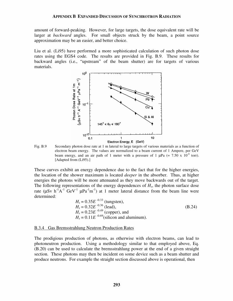
APPENDIX B EXPANDED DISCUSSION OF SYNCHROTRON RADIATION
293
amount of forward-peaking. However, for large targets, the dose equivalent rate will be larger at backward angles. For small objects struck by the beam, a point source approximation may be an easier, and better choice. Liu et al. (Li95) have performed a more sophisticated calculation of such photon dose rates using the EGS4 code. The results are provided in Fig. B.9. These results for backward angles (i.e., “upstream” of the beam shutter) are for targets of various materials.
Fig. B.9 Secondary photon dose rate at 1 m lateral to large targets of various materials as a function of
electron beam energy. The values are normalized to a beam current of 1 Ampere, per GeV beam energy, and an air path of 1 meter with a pressure of 1 µPa (= 7.50 x 10⁻⁹ torr). [Adapted from (Li95).]
These curves exhibit an energy dependence due to the fact that for the higher energies, the location of the shower maximum is located deeper in the absorber. Thus, at higher energies the photons will be more attenuated as they move backwards out of the target. The following representations of the energy dependences of Hs, the photon surface dose rate (µSv h-1A-1 GeV-1 µPa-1m-1) at 1 meter lateral distance from the beam line were determined:
Hs = 0.35E -0.33 (tungsten), Hs = 0.32E -0.36 (lead), (B.24) Hs = 0.23E -0.49 (copper), and Hs = 0.11E -0.69(silicon and aluminum).
B.3.4 Gas Bremsstrahlung Neutron Production Rates The prodigious production of photons, as otherwise with electron beams, can lead to photoneutron production. Using a methodology similar to that employed above, Eq. (B.20) can be used to calculate the bremsstrahlung power at the end of a given straight section. These photons may then be incident on some device such as a beam shutter and produce neutrons. For example the straight section discussed above is operational, then

APPENDIX B EXPANDED DISCUSSION OF SYNCHROTRON RADIATION
294
3.24 x 10⁻⁵ watts goes into the bremsstrahlung at that location. One might assume the beam shutter is made of tungsten. For this material Fig. 3.7 and Table 3.1 give a total photoneutron yield of 2.36 x 10⁹ neutrons s-1 W-1, so 7.65 x 10⁴ neutrons s-1 will be emitted if this bremsstrahlung power is incident on this device. Since the photoneutrons are isotropic and “point source” conditions are a good approximation, a flux density of 0.61 neutrons cm-2 s-1 is found at a distance of 1 meter without including the effects of any intervening shielding. For these giant resonance neutrons a conservative dose equivalent per fluence conversion factor is 3.2 x 10⁻⁴ µSv cm2. When applied here, a dose equivalent rate of dH/dt = 1.95 x 10⁻⁴ µSv s-1 = 0.70 µSv h-1 is realized. Neutrons from quasi-deuteron and photopion reactions are ignored in this estimate. Again, according to Liu and Vylet (Li01), these values are in reasonable agreement with measurement and more sophisticated calculations. Liu et al. (Li95) have given more detailed results for neutron production by gas bremsstrahlung incident on various materials provided here. Fig. B.10 provides these results. The left frame of this figure presents both the normalized neutron dose rates at 1 meter from the target and the neutron yield with the target as a function of target atomic number. These results are for targets with sufficient size (≈ 30 Xo long and 30 Xm in diameter) to generate maximal neutron yields. The right frame of this figure can be used to estimate results for shorter targets made of lead.
Fig. B.10 Left frame: Neutron dose rate at 1 meter away from a beamline device struck by gas
bremsstrahlung and the neutron yield within the device as a function of the atomic number of the device. The values are normalized to a beam current of 1 A, per GeV beam energy, and an air path of 1 meter with a pressure of 1 µPA. Right frame: Relative neutron yield as a function of the target length in units of radiation length for a cylindrical lead target 15 Molière units in radius struck by gas bremsstrahlung for 4 electron beam energies. [Adapted from (Li95).]
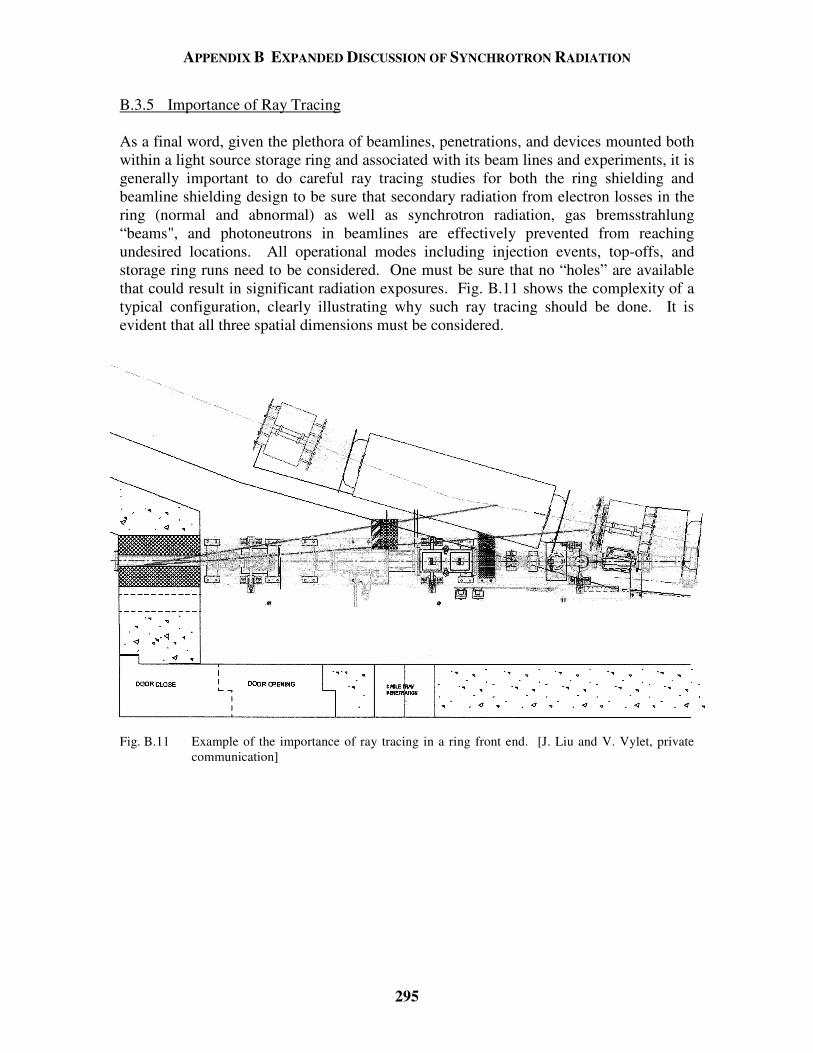
APPENDIX B EXPANDED DISCUSSION OF SYNCHROTRON RADIATION
295
B.3.5 Importance of Ray Tracing As a final word, given the plethora of beamlines, penetrations, and devices mounted both within a light source storage ring and associated with its beam lines and experiments, it is generally important to do careful ray tracing studies for both the ring shielding and beamline shielding design to be sure that secondary radiation from electron losses in the ring (normal and abnormal) as well as synchrotron radiation, gas bremsstrahlung “beams", and photoneutrons in beamlines are effectively prevented from reaching undesired locations. All operational modes including injection events, top-offs, and storage ring runs need to be considered. One must be sure that no “holes” are available that could result in significant radiation exposures. Fig. B.11 shows the complexity of a typical configuration, clearly illustrating why such ray tracing should be done. It is evident that all three spatial dimensions must be considered.
Fig. B.11 Example of the importance of ray tracing in a ring front end. [J. Liu and V. Vylet, private
communication]
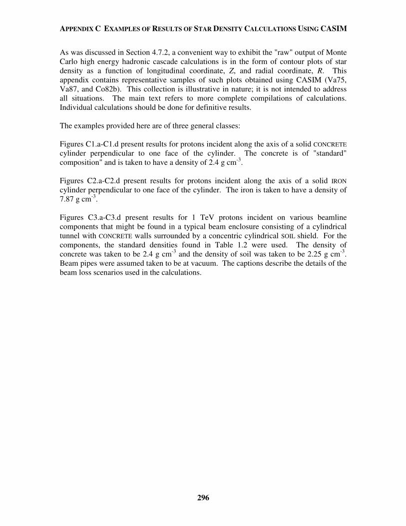
APPENDIX C EXAMPLES OF RESULTS OF STAR DENSITY CALCULATIONS USING CASIM
296
As was discussed in Section 4.7.2, a convenient way to exhibit the "raw" output of Monte Carlo high energy hadronic cascade calculations is in the form of contour plots of star density as a function of longitudinal coordinate, Z, and radial coordinate, R. This appendix contains representative samples of such plots obtained using CASIM (Va75, Va87, and Co82b). This collection is illustrative in nature; it is not intended to address all situations. The main text refers to more complete compilations of calculations. Individual calculations should be done for definitive results. The examples provided here are of three general classes: Figures C1.a-C1.d present results for protons incident along the axis of a solid CONCRETE cylinder perpendicular to one face of the cylinder. The concrete is of "standard" composition" and is taken to have a density of 2.4 g cm-3. Figures C2.a-C2.d present results for protons incident along the axis of a solid IRON cylinder perpendicular to one face of the cylinder. The iron is taken to have a density of 7.87 g cm-3. Figures C3.a-C3.d present results for 1 TeV protons incident on various beamline components that might be found in a typical beam enclosure consisting of a cylindrical tunnel with CONCRETE walls surrounded by a concentric cylindrical SOIL shield. For the components, the standard densities found in Table 1.2 were used. The density of concrete was taken to be 2.4 g cm-3 and the density of soil was taken to be 2.25 g cm-3. Beam pipes were assumed taken to be at vacuum. The captions describe the details of the beam loss scenarios used in the calculations.
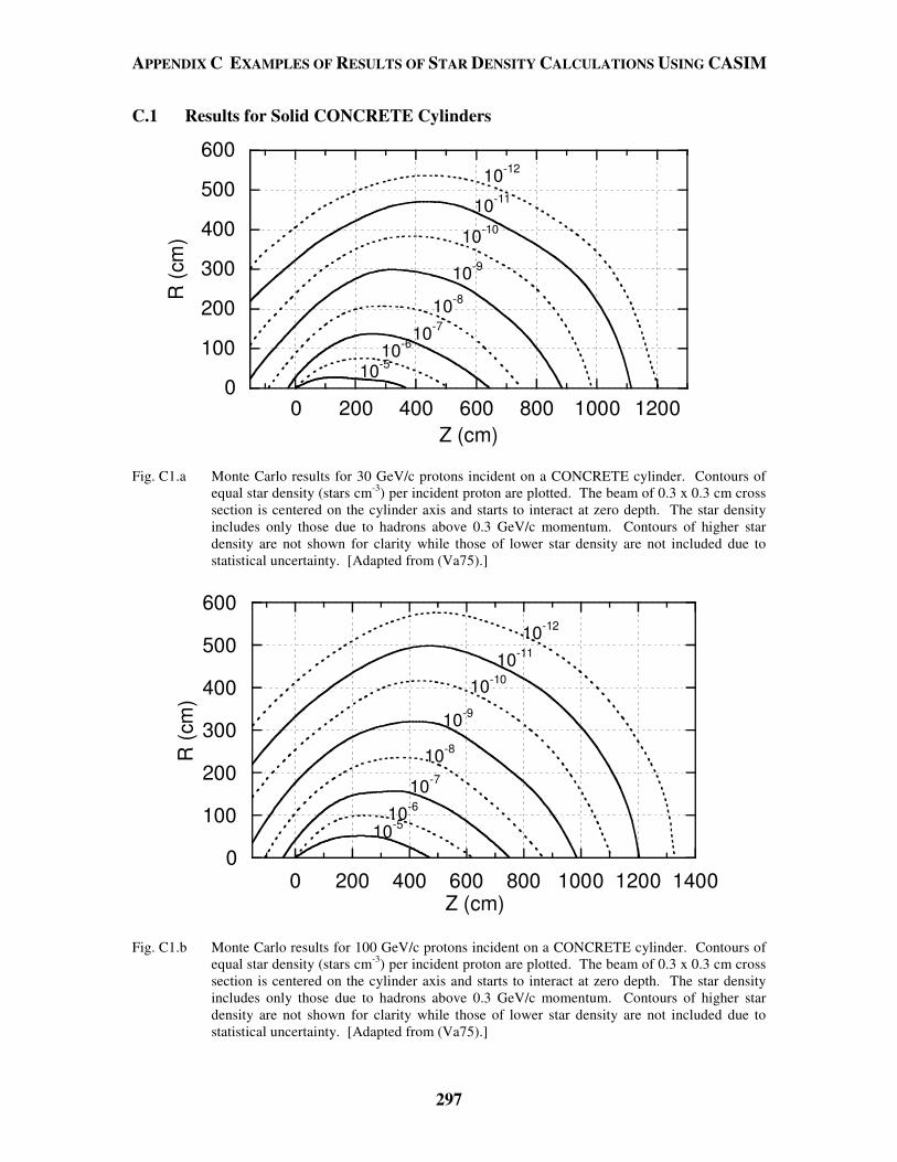
APPENDIX C EXAMPLES OF RESULTS OF STAR DENSITY CALCULATIONS USING CASIM
297
C.1 Results for Solid CONCRETE Cylinders
0
100
200
300
400
500
600
0 200 400 600 800 1000 1200
R (
cm)
Z (cm)
10-12
10-11
10-10
10-9
10-8
10-7
10-6
10-5
Fig. C1.a Monte Carlo results for 30 GeV/c protons incident on a CONCRETE cylinder. Contours of
equal star density (stars cm-3) per incident proton are plotted. The beam of 0.3 x 0.3 cm cross section is centered on the cylinder axis and starts to interact at zero depth. The star density includes only those due to hadrons above 0.3 GeV/c momentum. Contours of higher star density are not shown for clarity while those of lower star density are not included due to statistical uncertainty. [Adapted from (Va75).]
0
100
200
300
400
500
600
0 200 400 600 800 1000 1200 1400
R (
cm)
Z (cm)
10-510-6
10-7
10-8
10-9
10-1010-11
10-12
Fig. C1.b Monte Carlo results for 100 GeV/c protons incident on a CONCRETE cylinder. Contours of
equal star density (stars cm-3) per incident proton are plotted. The beam of 0.3 x 0.3 cm cross section is centered on the cylinder axis and starts to interact at zero depth. The star density includes only those due to hadrons above 0.3 GeV/c momentum. Contours of higher star density are not shown for clarity while those of lower star density are not included due to statistical uncertainty. [Adapted from (Va75).]
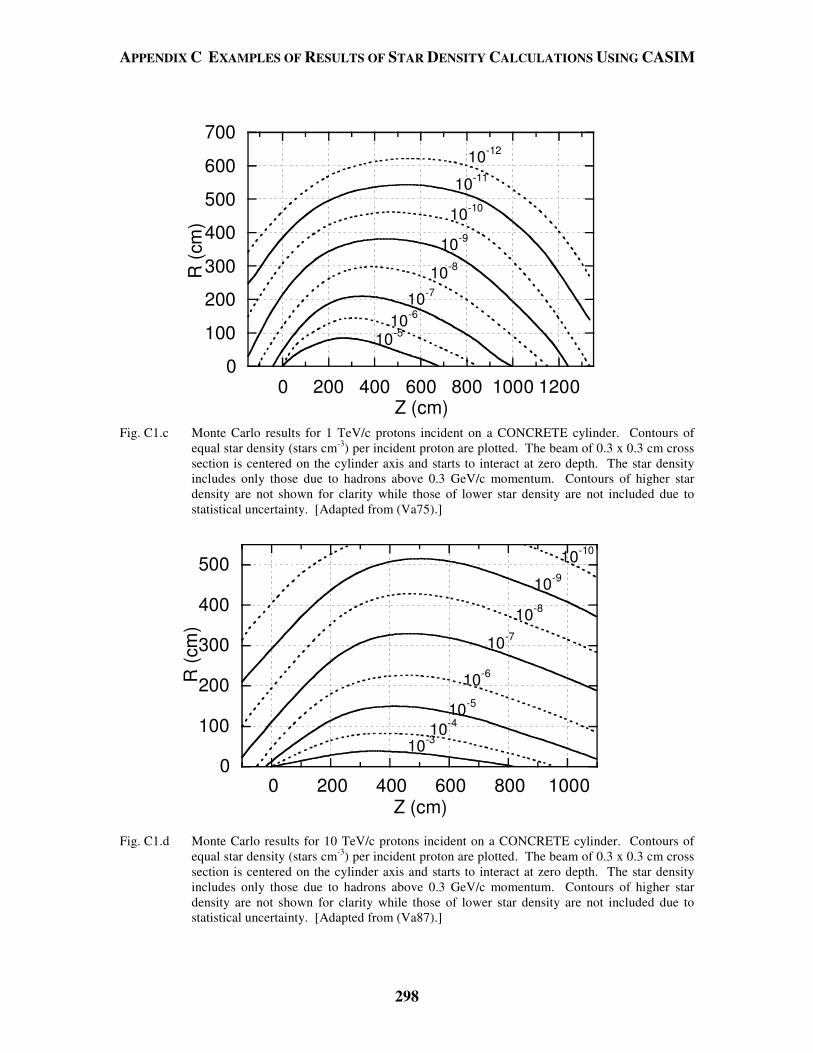
APPENDIX C EXAMPLES OF RESULTS OF STAR DENSITY CALCULATIONS USING CASIM
298
0
100
200
300
400
500
600
700
0 200 400 600 800 1000 1200
R (
cm)
Z (cm)
10-12
10-11
10-10
10-9
10-8
10-7
10-6
10-5
Fig. C1.c Monte Carlo results for 1 TeV/c protons incident on a CONCRETE cylinder. Contours of
equal star density (stars cm-3) per incident proton are plotted. The beam of 0.3 x 0.3 cm cross section is centered on the cylinder axis and starts to interact at zero depth. The star density includes only those due to hadrons above 0.3 GeV/c momentum. Contours of higher star density are not shown for clarity while those of lower star density are not included due to statistical uncertainty. [Adapted from (Va75).]
0
100
200
300
400
500
0 200 400 600 800 1000
R (
cm)
Z (cm)
10-10
10-8
10-9
10-7
10-6
10-5
10-4
10-3
Fig. C1.d Monte Carlo results for 10 TeV/c protons incident on a CONCRETE cylinder. Contours of
equal star density (stars cm-3) per incident proton are plotted. The beam of 0.3 x 0.3 cm cross section is centered on the cylinder axis and starts to interact at zero depth. The star density includes only those due to hadrons above 0.3 GeV/c momentum. Contours of higher star density are not shown for clarity while those of lower star density are not included due to statistical uncertainty. [Adapted from (Va87).]
APPENDIX C EXAMPLES OF RESULTS OF STAR DENSITY CALCULATIONS USING CASIM
299
C.2 Results for Solid IRON Cylinders
0
30
60
90
120
150
180
210
240
-100 0 100 200 300 400 500 600 700
R (
cm)
Z (cm)
10-12
10-11
10-10
10-9
10-8
10-7
10-6
10-5
10-4
Fig. C2.a Monte Carlo results for 30 GeV/c protons incident on an IRON cylinder. Contours of equal
star density (stars cm-3) per incident proton are plotted. The beam of 0.3 x 0.3 cm cross section is centered on the cylinder axis and starts to interact at zero depth. The star density includes only those due to hadrons above 0.3 GeV/c momentum. Contours of higher star density are not shown for clarity while those of lower star density are not included due to statistical uncertainty. [Adapted from (Va75).]
0306090
120150180210
240
-100 0 100 200 300 400 500 600 700 800
R (
cm)
Z (cm)
10-12
10-11
10-10
10-9
10-8
10-7
10-6
10-5
10-4
Fig. C2.b Monte Carlo results for 100 GeV/c protons incident on an IRON cylinder. Contours of equal
star density (stars cm-3) per incident proton are plotted. The beam of 0.3 x 0.3 cm cross section is centered on the cylinder axis and starts to interact at zero depth. The star density includes only those due to hadrons above 0.3 GeV/c momentum. Contours of higher star density are not shown for clarity while those of lower star density are not included due to statistical uncertainty. [Adapted from (Va75).]
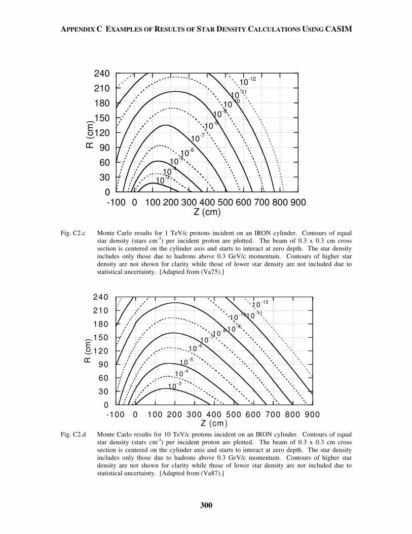
APPENDIX C EXAMPLES OF RESULTS OF STAR DENSITY CALCULATIONS USING CASIM
300
0
30
60
90
120
150
180
210
240
-100 0 100 200 300 400 500 600 700 800 900
R (
cm)
Z (cm)
10-3
10-12
10-11
10-10
10-9
10-8
10-7
10-6
10-5
10-4
Fig. C2.c Monte Carlo results for 1 TeV/c protons incident on an IRON cylinder. Contours of equal
star density (stars cm-3) per incident proton are plotted. The beam of 0.3 x 0.3 cm cross section is centered on the cylinder axis and starts to interact at zero depth. The star density includes only those due to hadrons above 0.3 GeV/c momentum. Contours of higher star density are not shown for clarity while those of lower star density are not included due to statistical uncertainty. [Adapted from (Va75).]
0
30
60
90
120
150
180
210
240
-100 0 100 200 300 400 500 600 700 800 900
R (
cm)
Z (cm )
10 -12
10 -1110 -10
10 -9
10 -8
10 -7
10 -6
10 -5
10 -4
10 -3
Fig. C2.d Monte Carlo results for 10 TeV/c protons incident on an IRON cylinder. Contours of equal
star density (stars cm-3) per incident proton are plotted. The beam of 0.3 x 0.3 cm cross section is centered on the cylinder axis and starts to interact at zero depth. The star density includes only those due to hadrons above 0.3 GeV/c momentum. Contours of higher star density are not shown for clarity while those of lower star density are not included due to statistical uncertainty. [Adapted from (Va87).]
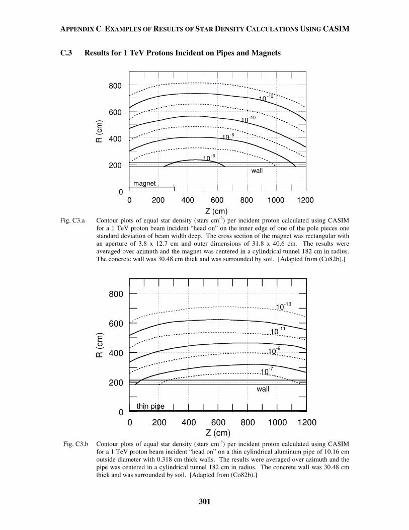
APPENDIX C EXAMPLES OF RESULTS OF STAR DENSITY CALCULATIONS USING CASIM
301
C.3 Results for 1 TeV Protons Incident on Pipes and Magnets
0
200
400
600
800
0 200 400 600 800 1000 1200
R (c
m)
Z (cm)
magnet
10 -6
10 -8
10 -10
10 -12
wall
Fig. C3.a Contour plots of equal star density (stars cm-3) per incident proton calculated using CASIM
for a 1 TeV proton beam incident “head on” on the inner edge of one of the pole pieces one standard deviation of beam width deep. The cross section of the magnet was rectangular with an aperture of 3.8 x 12.7 cm and outer dimensions of 31.8 x 40.6 cm. The results were averaged over azimuth and the magnet was centered in a cylindrical tunnel 182 cm in radius. The concrete wall was 30.48 cm thick and was surrounded by soil. [Adapted from (Co82b).]
0
200
400
600
800
0 200 400 600 800 1000 1200
R (c
m)
Z (cm)
10-7
10-9
10-11
10-13
thin pipe
wall
Fig. C3.b Contour plots of equal star density (stars cm-3) per incident proton calculated using CASIM
for a 1 TeV proton beam incident “head on” on a thin cylindrical aluminum pipe of 10.16 cm outside diameter with 0.318 cm thick walls. The results were averaged over azimuth and the pipe was centered in a cylindrical tunnel 182 cm in radius. The concrete wall was 30.48 cm thick and was surrounded by soil. [Adapted from (Co82b).]
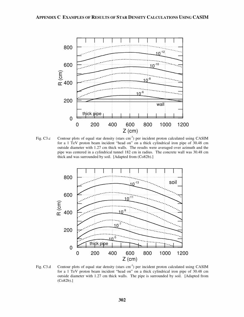
APPENDIX C EXAMPLES OF RESULTS OF STAR DENSITY CALCULATIONS USING CASIM
302
0
200
400
600
800
0 200 400 600 800 1000 1200
R (c
m)
Z (cm)
wall
thick pipe
10-6
10-8
10-10
10-12
Fig. C3.c Contour plots of equal star density (stars cm-3) per incident proton calculated using CASIM
for a 1 TeV proton beam incident “head on” on a thick cylindrical iron pipe of 30.48 cm outside diameter with 1.27 cm thick walls. The results were averaged over azimuth and the pipe was centered in a cylindrical tunnel 182 cm in radius. The concrete wall was 30.48 cm thick and was surrounded by soil. [Adapted from (Co82b).]
0
200
400
600
800
0 200 400 600 800 1000 1200
R (c
m)
Z (cm)
thick pipe
soil
10-5
10-9
10-7
10-11
10-13
Fig. C3.d Contour plots of equal star density (stars cm-3) per incident proton calculated using CASIM
for a 1 TeV proton beam incident “head on” on a thick cylindrical iron pipe of 30.48 cm outside diameter with 1.27 cm thick walls. The pipe is surrounded by soil. [Adapted from (Co82b).]
REFERENCES
303
(Aa86) P. A. Aarnio, A. Fassò, H. J. Moehring, J. Ranft, G. R. Stevenson, "FLUKA86 users guide", CERN Divisional Report TIS-RP/168 (European Organization for Nuclear Research, CERN, 1986).
(Al73) R. G. Alsmiller, Jr, and J. Barish, "Shielding against the neutrons
produced when 400 MeV electrons are incident on a thick copper target", Part. Accel. 5 (1973) 155-159.
(Al75) R. G. Alsmiller, R. T. Santoro, and J. Barish, "Shielding calculations for a
200 MeV proton accelerator and comparisons with experimental data", Part. Accel. 7 (1975) 1-7.
(Al81) R. G. Alsmiller, J. Barish, and R. L. Childs, "Skyshine at neutron energies
< 400 MeV", Part. Accel. 11 (1981) 131-141. (Al85) V. E. Aleinikov, A. P. Cherevatenko, F. B. Clapier, and V. I. Tsovbun,
"Neutron radiation field due to 6.6 MeV/amu 58Ni ions bombarding a thick Cu target", Rad. Prot. Dos. 11 (1985) 245-248.
(An62) I. O. Andersson and J. Braun, "A neutron rem counter", Nucleonik 6
(1963) 237 and I. O. Andersson and J. Braun, "A neutron rem counter with uniform sensitivity from 0.025 MeV to 10 MeV", Neutron dosimetry, (Proceedings of a Symposium held at Harwell, 1962) vol. 2, p.87.
(An07) M. P. Anderson, Introducing groundwater physics, Phys. Today (May
2007) 42-47. (Ap79) R. E. Apfel, "The superheated drop detector", Nucl. Instr. and Meth. 162
(1979) 603-608. (Ar69a) T. W. Armstrong and R. G. Alsmiller, Jr., "Calculation of the residual
photon dose rate around high energy proton accelerators", Nucl. Sci. Eng. 38 (1969) 53-62.
(Ar69b) T. W. Armstrong and J. Barish, "Calculation of the residual photon dose
rate due to the activation of concrete by neutrons from a 3-GeV proton beam in iron", in Proceedings of the second international conference on accelerator radiation dosimetry and experience, (Stanford, CA 1969).
(Ar80) T. W. Armstrong, "The HETC hadronic cascade code", in Computer techniques in radiation transport and dosimetry, W. R. Nelson and T. M. Jenkins, editors (Plenum Press, New York and London 1980), pp. 373-375.
REFERENCES
304
(Ar97) A. Aroua, T. Buchillier, M. Gracescu, and M. Höfert, "Neutron measurements around a high-energy lead ion beam at CERN", Rad. Prot. Dos. 70 (1997) 437-440.
(Aw72) M. Awschalom, "Bonner spheres and tissue equivalent chambers for
extensive radiation area monitoring around a 1/2 TeV proton synchrotron", in Proceedings of IAEA Symposium on neutron monitoring for radiation protection purposes (Vienna, 1972, vol 1, p. 297). The details of the measurements are discussed in M. Awschalom, T. Borak, and H. Howe, "A study of spherical, pseudospherical, and cylindrical moderators for a neutron dose equivalent rate meter", Fermilab Report TM-291 (Fermi National Accelerator Laboratory, July 1971).
(Aw73) M. Awschalom and L. Coulson, "A new technique in environmental
neutron spectroscopy", in Proceedings of the third international conference of the International Radiation Protection Association, Washington, DC, 1973 (U. S. Atomic Energy Commission, Technical Information Center, Oak Ridge Tennessee, CONF 730907-P2).
(Aw85) M. Awschalom and R. S. Sanna, "Applications of Bonner sphere detectors
in neutron field dosimetry", Rad. Prot. Dos. 10 (1985) 89-101. (Ba65) J. Baarli and A. H. Sullivan, "Radiation dosimetry for protection purposes
near high energy particle accelerators", Health Phys. 11 (1965) 353-361. (Ba67) G. Bathow, E. Freytag, and K. Tesch, "Measurements on 6.3 GeV
electromagnetic cascades and cascade producing neutrons", Nucl. Phys. B2 (1967) 669-689.
(Ba69) M. Barbier, Induced radioactivity (North-Holland Publishing Company,
Amsterdam and London, Wiley Interscience Division, John Wiley and Sons, Inc, New York, 1969).
(Ba84) S. I. Baker, C. R. Kerns, S. H. Pordes, J. B. Cumming, A. Soukas, V.
Agoritsas, and G. R. Stevenson, "Absolute cross section for the production of 24Na in Cu by 400 GeV protons", Nucl. Instr. and Meth. A222 (1984) 467-473.
(Ba89) S. Ban, H. Hirayama, and S. Muiri, "Estimation of absorbed dose due to
gas bremsstrahlung from electron storage rings", Health Phys. 57 (1989) 407-412.
(Ba91) S. I. Baker, R. A. Allen, P. Yurista, V. Agoritsas, and J. B. Cumming,
"Cu(p, x)24Na cross section from 30 to 800 GeV", Phys. Rev. C43 (1991) 2862-2865.
REFERENCES
305
(Ba98) V. Batu, Aquifer hydraulics (John Wiley and Sons, Inc., New York, 1998). (Be70) M. J. Berger and S. M. Seltzer, "Bremsstrahlung and photoneutrons from
thick tunsten and tantalum targets", Phys. Rev. C2 (1970) 621-631. (Bo72) T. B. Borak, M. Awschalom, W. Fairman, F. Iwami, and J. Sedlet, "The
underground migration of radionuclides produced in soil near high energy proton accelerators", Health Phys. 23 (1972) 679-687.
(Bo87) T. B. Borak and J. W. N. Tuyn, "Can uranium calorimeters become
critical? ", CERN Report TIS-RP/194 (European Organization for Nuclear Research, 1987).
(Br60) R. L. Bramblett, R. I. Ewing, and T. W. Bonner, "A new type of neutron
dosimeter", Nucl. Instr. and Meth. 9 (1960) 1-12. (Br78) L. W. Brackenbush, G. W. R. Endres, and L. G. Faust, "Measuring
neutron dose and quality factors with tissue-equivalent proportional counters", in Advances in radiation monitoring, proceedings of a symposium (IAEA, Stockholm, 1978).
(Br97) J. F. Briesmeister, Editor, "MCNP: A general Monte Carlo N-particle
transport code", LANL Report LA-12625-M, Version 4B (Los Alamos National Laboratory, March 1997).
(Br99) G. I. Britvich, A. A. Chumakov, R. M. Ronningen, R. A. Blue, and L. H.
Heilbronn, “Measurements of thick target neutron yields and shielding studies using beams of 4He, 12C, and 16O at 155 MeV/nucleon from the K1200 cyclotron at the National Superconducting Cyclotron Laboratory", Rev. Sci. Instr. 70 (1999) 2314-2314.
(Bu89) S. W. Butala, S. I. Baker, and P. M. Yurista, "Measurements of radioactive
gaseous releases to air from target halls at a high-energy proton accelerator", Health Phys. 57 (1989) 909-916.
(Ca87) D. C. Carey, The optics of charged particle beams (Harwood Academic
Publishers, New York 1987). (Ce69) H. Cember, Introduction to health physics (Pergamon Press, New York,
1969). Second and third editions of this classic text have been produced. (Ce80) R. A. Cecil, B. D. Anderson, A. R. Baldwin, R. Madey, A. Galonsky, P.
Miller, L. Young, and F. M. Waterman, "Neutron angular and energy distributions from 710-MeV alphas stopping in water, carbon, steel, and lead, and 640-MeV alphas stopping in lead", Phys. Rev. C21 (1980) 2470-2484.
REFERENCES
306
(CFR76) United States Code of Federal Regulations, Title 40, Part 141.16, "National primary drinking water standard for beta- and gamma- emitting radionuclides", 1976.
(CFR89) United States Code of Federal Regulations, Title 40, Part 61, Subpart H,
"National emissions standard for hazardous air pollutants (NESHAP) for the emission of radionuclides other than radon from Department of Energy Facilities", 1989.
(CFR93) United States Code of Federal Regulations, Title 10 Part 835,
"Occupational radiation protection at department of energy facilities", 1993. These Regulations were amended in November 1998.
(CFR00) United States Code of Federal Regulations, Title 40, Parts 9, 141, and 142,
"National primary drinking water regulations; final rule", December 2000. (Ch63) A. B. Chilton and C. M. Huddleston, "A semi-empirical formula for
differential dose albedo for gamma rays on concrete", Nucl. Sci. Eng. 17 (1963) 419.
(Ch64) A. B. Chilton, "Backscatter for gamma rays from a point source near a
concrete plane surface", Univ. Illinois Eng. Sta. Bull. No 471 (University of Illinois, Urbana, Illinois, 1964).
(Ch65a) A. B. Chilton, "Backscattering of gamma rays from point sources by an
infinite-plane concrete surface", Nucl. Sci. Eng. 21 (1965) 194-200. (Ch65b) A. B. Chilton, C. M. Davisson, and L. A. Beach (1965), "Parameters for
C-H albedo formula for gamma rays reflected from water, concrete, iron, and lead", Trans. Am. Nucl. Soc. 8, No. 2, (1965) 656-657.
(Ch84) A. B. Chilton, J. K. Shultis, and R. E. Faw, Principles of radiation
shielding (Prentice-Hall, Englewood Cliffs, New Jersey, 1984). (Ch99) A. W. Chao and M. Tigner, editors, Handbook of accelerator physics and
engineering (World Scientific Publishing Co., Singapore, 1999). (Ci65) A. Citron, L. Hoffmann, C. Passow, W. R. Nelson, and M. Whitehead, "A
study of the nuclear cascade in steel initiated by 19.2 GeV/c protons", Nucl. Instrum. Meth. 32 (1965) 48-52.
(Cl71) F. H. Clark, "Shielding Data" Appendix E, in Protection against neutron
radiation, NCRP Report No. 39 (National Council on Radiation Protection and Measurements, Washington, DC, 1971).
REFERENCES
307
(Cl83) F. Clapier and C. S. Zaidins, "Neutron dose equivalent rates due to heavy ion beams", Nucl. Instr. and Meth. 217 (1983) 489-494.
(Co73) M. O. Cohen, W. Guber, E. S.Troubezkoy, H. Lichtenstein, and H. A.
Steinberg, "SAM-CE, a three dimensional Monte-Carlo code for the solution of the forward neutron and forward and adjoint gamma ray transport equations", Rept. DNA-2830-F, Rev. B Defense Nuclear Agency, Washington, DC (1973).
(Co78) B. L. Cohen, "Nuclear cross sections", Handbook of radiation
measurement and protection, Section A: Volume I Physical science and engineering data, A. Brodsky, editor (CRC Press, Inc., West Palm Beach, Florida, 1978).
(Co82a) J. D. Cossairt, N. V. Mokhov, and C. T. Murphy, "Absorbed dose
measurements external to thick shielding at a high energy proton accelerator: Comparison with Monte-Carlo calculations", Nucl. Instr. and Meth. 197 (1982) 465-472.
(Co82b) J. D. Cossairt, "A collection of CASIM calculations", Fermilab Report
TM-1140 (Fermi National Accelerator Laboratory, 1982). (Co83) J. D. Cossairt, "Recent muon fluence measurements at Fermilab", Health
Phys. 45 (1983) 651-658. (Co84) J. D. Cossairt, D. W. Grobe, and M. A. Gerardi, "Measurements of
radiation quality factors using a recombination chamber", Fermilab Report TM-1248 (Fermi National Accclerator Laboratory, 1984).
(Co85a) J. D. Cossairt, S. W. Butala, and M. A. Gerardi, "Absorbed dose
measurements at an 800 GeV proton accelerator, comparison with Monte-Carlo calculations”, Nucl. Instr. and Meth. in Phys. Res. A238 (1985) 504-508.
(Co85b) J. D. Cossairt, J. G. Couch, A. J. Elwyn, and W. S. Freeman, "Radiation
measurements in a labyrinth penetration at a high-energy proton accelerator", Health Phys. 49 (1985) 907-917.
(Co85c) J. D. Cossairt and L. V. Coulson, "Neutron skyshine measurements at
Fermilab", Health Phys. 48 (1985) 171-181. (Co87) J. D. Cossairt and A. J. Elwyn, "Personal dosimetry in a mixed field of
high-energy muons and neutrons", Health Phys. 52 (1987) 813-818.
REFERENCES
308
(Co88) J. D. Cossairt, A. J. Elwyn, W. S. Freeman, W. C. Salsbury, and P. M. Yurista, "Measurement of neutrons in enclosures and outside of shielding at the Tevatron", Report Fermilab-Conf-88/106 (1988) also in Proceedings of the 22nd midyear meeting of the Health Physics Society; Topical meeting on instrumentation, San Antonio, TX, December, 1988, pp. 190-199.
(Co89a) J. D. Cossairt, A. J. Elwyn, W. S. Freeman, and S. W. Butala, "A study of
the transport of high energy muons through a soil shield at the Tevatron", Nucl. Instr. and Meth. in Phys. Res. A276 (1989) 78-85.
(Co89b) J. D. Cossairt, A. J. Elwyn, and W. S. Freeman, "A study of the production
and transport of high energy muons through a soil shield at the Tevatron", Nucl. Instr. and Meth. in Phys Res. A276 (1989) 86-93.
(Co95) J. D. Cossairt, "Approximate technique for estimating labyrinth
attenuation of accelerator-produced neutrons", Fermilab Radiation Physics Note No. 118 (Fermi National Accelerator Laboratory, October 1995).
(Co96) J. D. Cossairt, "On residual dose rate within particle accelerator
enclosures", Health Phys. 71 (1996) 315-319. (Co97) J. D. Cossairt, N. L. Grossman, and E. T. Marshall, "Assessment of dose
equivalent due to neutrinos", Health Phys. 73 (1997) 894-898. (Co98) J. D. Cossairt, "Rule of thumb for estimating groundwater activation from
residual dose rates", Fermilab Environmental Protection Note No. 15 (Fermi National Accelerator Laboratory, June 1998).
(Cu55) S. C. Curran, "Proportional counter spectroscopy", in Beta and gamma-
ray spectroscopy, K. Siegbahn, editor (Elsevier-North Holland, Amsterdam (1955).
(De65) H. DeStaebler, "Similarity of shielding problems at electron and proton
accelerators", SLAC Report SLAC Pub. 179 (Stanford Linear Accelerator Center, 1965). These results are also quoted in (Sc90).
(DeP66) J. DePangher and L. L. Nichols, "A precision long counter for measuring
fast neutron flux density", PNL Report BNWL-260 (Pacific Northwest Laboratory, 1966).
(D'H68) M. M. D'Hombres, C. Devillers, F. Gervaise, B. De Sereville, and P.
Tardy-Joubert, "Propagation des neutrons dans les tunnes d'Accès à un accélérateur de haute energie à protons", Rep. CEA-R-3491 (Centre d'études nucléaires de Saclay, 1968).
REFERENCES
309
(DOE90) U. S. Department of Energy Order 5400.5, "Radiation protection of the public and the environment" (1990). Subsequent revisions to this Order have been made.
(Ed93) D. A. Edwards and M. J. Syphers, An introduction to the physics of high
energy accelerators (John Wiley and Sons, Inc., New York, 1993). (El86) A. J. Elwyn and J. D. Cossairt, "A study of neutron leakage through an Fe
shield at an accelerator", Health Phys. 51 (1986) 723-735. (El91) A. J. Elwyn to J. D. Cossairt, private communication (1991). (En66) H. A. Enge, Introduction to nuclear physics (Addison-Wesley, Reading,
Massachusetts, 1966). (Fa84) A. Fassò, K. Goebel, M. Höfert, G. Rau, H. Schönbacher, G. R.
Stevenson, A. H. Sullivan, W. P. Swanson, and J. W. N. Tuyn, "Radiation problems in the design of the large electron-positron collider (LEP)", CERN Report 84-02 (European Organization for Nuclear Research, 1984).
(Fa93) A. Fassò, A. Ferrari, J. Ranft, P.R. Sala, "FLUKA: present status and
future developments", in Proc. IV Int. Conf. on calorimetry in high energy physics, La Biodola, Italy, 21-26 Sept. 1993, Ed. A. Menzione and A. Scribano, p. 493 (World Scientific Publishing Co, Singapore, 1993).
(Fe88) C. W. Fetter, Applied hydrogeology (Merrill Publishing Company,
Columbus, OH, 1988). (Fr84) W. S. Freeman and F. P. Krueger, "Neutron calibration tests of Fermilab
radiation detectors", Fermilab Radiation Physics Note No. 48 (Fermi National Accelerator Laboratory, 1984).
(Ga73) T. A. Gabriel and R. T. Santoro, "Photon dose rates from the interactions
of 100 GeV protons in iron and iron-lead beam stops", Part. Accel. 4 (1973) 169-186.
(Ga85) T. A. Gabriel, "The high energy transport code HETC", Oak Ridge
National Laboratory Report ORNL-TM-9727 (1985). (Ga94) T. A. Gabriel, D. E. Groom, P. K. Job, N. V. Mokhov, and G. R.
Stevenson, "Energy dependence of hadronic activity", Nucl. Instrum. and Meth. in Phys. Res. A338 (1994) 336-347.
(Gi68) W. S. Gilbert, et al, "1966 CERN-LRL-RHEL shielding experiment at the
CERN proton synchrotron", UCRL-17941 (1968). Much of this material is summarized in (Pa73).
REFERENCES
310
(Gi69) W. S. Gilbert, "Shielding measurements at the CERN 25 GeV proton synchrotron", Rept. CONF-691101, USAEC 323 (1969).
(Go71) P. J. Gollon and M. Awschalom, "Design of penetrations in hadron
shields", CERN Report 71-16 Vol. 2 (1971) also published in IEEE Trans. Nucl. Sci NS-18 (1971) 741-745.
(Go75) K. Goebel, G. R. Stevenson, J. T. Routti, and H. G. Vogt, "Evaluating
dose rates due to neutron leakage through the access tunnels of the SPS", CERN Report LABII-RA/Note/75-10 (European Organization for Nuclear Research, 1975).
(Go76) P. J. Gollon, "Production of radioactivity by particle accelerators",
Fermilab Report TM-609 (Fermi National Accelerator Laboratory, 1976) and also IEEE Trans. Nucl. Sci. NS 23 No. 4 (1976) 1395-1400.
(Go78) P. J. Gollon, "Soil activation calculations for the anti-proton target area",
Fermilab Report TM-816 (Fermi National Accelerator Laboratory, 1978). (Gr85) R. V. Griffith, and J. H. Thorngate, "Neutron spectrometers for radiation
monitoring at Lawrence Livermore National Laboratory", Rad. Prot. Dos. 10 (1-4) (1985) 125-135.
(Gr87) N. A. Greenhouse, T. M. De Castro, J. B. McCaslin, A. R. Smith, R.-K.
Sun, and D. E. Hankins, "An evaluation of NTA film in an accelerator environment and comparisons with CR-39", Rad. Prot. Dos. 20 (1987) 143-147.
(Gr90) R. V. Griffith and L. Tommasino, in "Dosimetry for radiological
protection at high energy particle accelerators", Chapter 1 in The dosimetry of ionizing radiation, Volume IV (K. R. Kase, B. E. Bjärngard, and F. H. Attix, editors, Academic Press, 1990).
(Ha47) A. O. Hanson and M. L. McKibben, "A neutron detector having uniform
sensitivity from 10 keV to 3 MeV", Phys. Rev. 72 (1947) 673-677. (Ha62) D. E. Hankins, "Neutron monitoring instrument having a response
approximately proportional to the dose rate from thermal to 7.0 MeV", Los Alamos Scientific laboratory Report LA-2717 (Los Alamos Scientific Laboratory, 1962).
(Ha88) W. K. Hagan, B. L. Colborn, T. W. Armstrong, and M. Allen, "Radiation
shielding calculations for a 70-250 MeV proton therapy facility", Nucl. Sci. Eng. 98 (1988) 272-278.

REFERENCES
311
(He85) N. E. Hertel and J. W. Davidson, "The response of Bonner spheres to neutrons from thermal energies to 17.3 MeV", Nucl. Instr. and Meth. in Phys. Res. A238 (1985) 509-516.
(He99) L. Heilbronn, R. S. Cary, M. Cronqvist, F. Deák, K. Frankel, A. Galonsky,
K. Holabird, Á. Horvath, Á. Kiss, J. Kruse, R. M. Ronningen, H. Schelin, and Z. Seres, "Neutron yields from 155 MeV/nucleon carbon and helium stopping in aluminum", Nucl. Sci. and Eng. I32 (1999)1-15.
(Hö69) M. Höfert, "Radiation hazard of induced activity in air as produced by
high energy accelerators", in Proceedings of the second international conference on accelerator radiation dosimetry and experience (Stanford, CA 1969). Important results from this work are also found in (Sw79a).
(Hö80) M. Höfert and Ch. Raffnsøe, "Measurement of absolute absorbed dose and
dose equivalent response for instruments used around high-energy proton accelerators", Nucl. Instr. and Meth. 176 (1980) 443-448.
(Hö84a) M. Höfert and G. R. Stevenson, "The assessment of dose equivalent in
stray radiation fields around high-energy accelerators", CERN Report TIS-RP/131/CF (European Organization for Nuclear Research, 1984).
(Hö84b) M. Höfert, "The NTA emulsion: an ill-reputed but misjudged neutron
detector", in Pacific Northwest Laboratory Report PNL-SA 12352 (CONF-8308140, 1984) or CERN Report TIS-RP/110/CF (1984).
(Hu60) E. L. Hubbard, R. M. Main, and R. V. Pyle, "Neutron production by
heavy-ion bombardments", Phys. Rev. 118 (1960) 507-514. (IC71) International Commission on Radiation Units and Measurements,
Radiation protection instrumentation and its application, ICRU Publication 20 (ICRU, Bethesda, MD, 1971).
(IC73) International Commission on Radiological Protection, Data for protection
against ionizing radiation from external sources, supplement to ICRP Publication 15, ICRP Publication 21 (ICRP, Washington, DC, 1973).
(IC78) International Commission on Radiation Units and Measurements, Basic
aspects of high-energy particle interactions and radiation dosimetry, ICRU Report No. 28 (ICRU, Washington, DC, 1978).
(IC87) International Commission on Radiological Protection, Data for use in
protection against external radiation, ICRP Report No. 51 (1987).
REFERENCES
312
(IC91) International Commission on Radiological Protection, 1990 Recommendations of the International Commission on Radiological Protection, ICRP Report 60 (Pergamon Press, New York, 1991).
(In84) H. Ing and H. C. Birnboim, "A bubble-damage polymer detector for
neutrons", Nuclear Tracks Radiation Measurements, 8, No 1.4 (1984) 285-288.
(Ip94) N. E. Ipe and A. Fassò, "Gas bremsstrahlung considerations in the
shielding design of the Advanced Photon Source synchrotron radiation beam lines", Nucl. Instr. and Meth. A351 (1994) 534-544.
(Ja68) R. G. Jaeger, Editor-in-chief, E. P. Blizard, A. B. Chilton, M. Grotenhuis,
A. Hönig, Th. A. Jaeger, H. H. Eisenlohr, Engineering compendium on radiation shielding, Volume 1 Shielding fundamentals and methods (Springer-Verlag, New York, 1968).
(Ja75) J. D. Jackson, Classical electrodynamics, 2nd edition (John Wiley and
Sons, New York, 1975). Subsequent editions of this standard text have been published.
(Ja87) J. D. Jackson, editor, M. G. D. Gilchriese, D. E. Groom, J. R. Sanford, G.
R. Stevenson, W. S. Freeman, K. O'Brien, R. H. Thomas, "SSC environmental radiation shielding", Superconducting Super Collider Central Design Group Report SSC-SR-1026 (1987).
(Ka89) A.N. Kalinovskii, N.V. Mokhov, and Yu.P. Nikitin, in Passage of high-
energy particles through matter (American Institute of Physics, NY, 1989).
(Kn79) G. F. Knoll, Radiation detection and measurement (John Wiley and Sons,
New York, 1979). Subsequent editions of this classic text have been published.
(Ko81) E. J. Konopinski, Electromagnetic fields and relativistic particles
(McGraw Hill, New York, 1981). (Ko85) T. Kosako, T. Nakamura, and S. Iwai, "Estimation of response functions
of moderating type neutron detectors by the time-of-flight method combined with a large lead pile", Nucl. Instr. and Meth. in Phys. Res. A235 (1985) 103-122.
(Ko93) A. Yu. Konobeyev and Yu. A. Korovin, "Tritium production in materials
from C to Bi irradiated with nucleons of intermediate and high energies", Nucl. Instrm. and Meth. in Phys. Res. B82 (1993) 103-115.
REFERENCES
313
(Kr97) O.E. Krivosheev and N.V. Mokhov, "A new MARS and its applications' ", Fermilab-Conf-98/043 (1998) and SARE3 KEK Proceedings 97-5 (1997).
(Kr02) F. Krueger and J. Larson, "Chipmunk IV: Development of and experience
with a new generation of radiation area monitors for accelerator applications", Nucl. Instrm. and Meth. in Phys. Res A495 (2002) 20-28.
(Ku99) T. Kurosawa, N. Nakao, T. Nakamura, Y. Uwamino, T. Shibata, N.
Nakanishi, A. Fukumura, and K. Murakami, "Measurements of secondary neutrons produced from thick targets bombarded by high-energy helium and carbon ions", Nucl. Sci. and Eng. I32 (1999) 30-57.
(Ku00) T. Kurosawa, N. Nakao, T. Nakamura, H. Iwase, H. Sato, Y. Uwamino,
and A. Fukumura, "Neutron yields from thick C, Al, Cu, and Pb targets bombarded by 400 MeV/nucleon Ar, Fe, Xe, and 800 MeV/nucleon Si ions", Phys Rev C62 (2000) 044615 (11 pages).
(Le68) J. W. Leake, "An improved spherical dose equivalent neutron detector",
Nucl. Instrum. and Meth. 63 (1968) 329-332. (Le72) G. S. Levine, D. M. Squier, G. B. Stapleton, G. R. Stevenson, K. Goebel,
and J. Ranft, "The angular dependence of dose and hadron yields from targets in 8 GeV/c and 24 GeV/c extracted beams", Part. Acc. 3 (1972) 91-101.
(Li61) S. J. Lindenbaum, "Shielding of high energy accelerators", Ann. Rev.
Nucl. Sci. 11 (1961) 213-258. (Li95) J. C. Liu, W. R. Nelson, and K. R. Kase, "Gas bremsstrahlung and
associated photon-neutron shielding calculations for electron storage rings", Health Phys. 68 (1995) 105-213.
(Li01) J. C. Liu and V. Vylet, "Radiation protection at synchrotron radiation
facilities", Rad. Prot. Dos. 96 (2001) 345-357. (Li05) J. C. Liu, A. Fassò, H. Khater, A. Prinz, and S. H. Rokni, "Radiation
safety design for SPEAR3 Ring and synchrotron radiation beamlines", SLAC Internal Report, Radiation Protection Department, Stanford Linear Acclerator Center, Stanford CA, USA, to be submitted to Nucl. Instrum. and Meth. (2005).
REFERENCES
314
(Lo84) K. A. Lowry and T. L. Johnson, "Modifications to interactive recursion unfolding algorithms and computer codes to find more appropriate neutron spectra", U. S. Naval Research Laboratory Report NRL-5430, Washington, DC (1984) and L. W. Brackenbush and R. I. Scherpelz, "SPUNIT: a computer code for multisphere unfolding", in Proc. of the Health Physics Society topical meeting on computer applications in health physics (Columbia Chapter of the Health Physics Society, Richland, WA, 1984).
(Ma67) R. E. Maerker and V. R. Cain, "AMC, a Monte-Carlo code utilizing the
albedo approach for calculating neutron and capture gamma-ray distributions in rectangular concrete ducts", Report ORNL-3964 (Oak Ridge National Laboratory, 1967).
(Ma68) J. B. Marion and F. C. Young, Nuclear reaction analysis, graphs and
tables (North Holland, Amsterdam, 1968). (Ma88) G. Margaritondo, Introduction to synchrotron radiation (Oxford
University Press, New York, 1988). (Ma93) A. J. Malensek, A. A. Wehmann, A. J. Elwyn, K. J. Moss, and P. M.
Kesich, "Groundwater migration of radionuclides at Fermilab", Fermilab Report TM-1851 (Fermi National Accelerator Laboratory, 1993).
(McC60) J. B. McCaslin, "A high-energy neutron-flux detector", Health Phys. 2
(1960) 399-407. (McC68) J. B. McCaslin, H. W. Patterson, A. R. Smith, and L. D. Stephens, "Some
recent developments in technique for monitoring high-energy accelerator radiation", In Proc. of the first international congress of radiation protection, International Radiation Protection Association, Pergamon Press, New York, Part 2 (1968) 1131-1137.
(McC85) J. B. McCaslin, P. R. LaPlant, A. R. Smith, W. P. Swanson, and R. H.
Thomas, "Neutron production by Ne and Si ions on a thick Cu target at 670 MeV/A with application to radiation protection", IEEE Trans. on Nucl. Sci. NS-32, No. 5 (1985) 3104-3106.
(McC87) J. B. McCaslin, W. P. Swanson, and R. H. Thomas, "Moyer model
approximations for point and extended beam losses", Nucl. Instr. and Meth. in Phys. Res. A256 (1987) 418-426.
REFERENCES
315
(McC88) J. B. McCaslin, R.-K. Sun, W. P. Swanson, J. D. Cossairt, A. J. Elwyn, W. S. Freeman, H. Jöstlein, C. D. Moore, P. M. Yurista, and D. E. Groom, "Radiation environment in the tunnel of a high-energy proton accelerator at energies near 1 TeV", Lawrence Berkeley Report LBL-24640 (1987), presented at the Seventh Annual Congress of the International Radiation Protection Association, Sydney, Australia, April, 1988.
(Mo86) N. V. Mokhov and J. D. Cossairt, "A short review of Monte Carlo
hadronic cascade calculations in the multi-TeV energy region", Nucl. Instr. and Meth. in Phys. Res. A244 (1986) 349-355.
(Mo89) L. E. Moritz, "Measurement of neutron leakage spectra at a 500 MeV
proton accelerator", Health Phys. 56 (1989) 287-296. (Mo95) N.V. Mokhov, "The MARS code system user's guide, version 13",
Fermilab Report FN-628 (Fermi National Accelerator Laboratory, 1995), http://www-ap.fnal.gov/MARS/.
(Mo97) N. Mokhov, private communication (1997). (Mo99) N. V. Mokhov and A. Van Ginneken, "Neutrino induced radiation at muon
colliders", presented at the 1999 Particle Accelerator Conference, New York, New York, March 19-April 2, 1999, Fermilab Report, FERMILAB-Conf-99-067 (Fermi National Accelerator Laboratory, 1999).
(Mo04) N. V. Mokhov, K. K. Guidima, C. C. James, M. A. Kostin, S. G. Mashnik,
E. Ng, J.-F. Ostiguy, I. L. Rakhno, A. J. Sierk, and S. I. Striganov, "Recent enhancements to the MARS15 Code", Fermilab Report FERMILAB-Conf-04/053-AD (Fermi National Accelreator Laboratory, 2004).
(Na78) T. Nakamura, M. Yoshida, and T. Shin, "Spectra measurements of
neutrons and photons from thick targets of C, Fe, Cu, and Pb by 52 MeV protons", Nucl. Instr. and Meth. 151 (1978) 493-503.
(Na81) T. Nakamura and T. Kosako, "A systematic study on neutron skyshine
from nuclear facilities, Part I: Monte-Carlo analysis of neutron propagation in air-over-ground environment from a monoenergetic source", Nucl. Sci, and Eng. 77 (1981) 168-181.
(Na85) T. Nakamura, "Neutron energy spectra produced from thick targets by
light-mass heavy ions”, Nucl. Instr. and Meth. in Phys. Res. A240 (1985) 207-215.
(Na05) T. Nakamura and L. Heilbronn, Handbook on secondary particle
production and transport by high-energy heavy ions (World Scientific Publishing Co., Singapore, 2005).
REFERENCES
316
(NC77) E. A. Burrill, Chair, J. R. Beyster, G. L. Brownell, A. B. Chilton, J. Haimson, C. J. Karzmark, W. E. Kreger, J, M. Wyckoff, Radiation protection design guidelines for 0.1-100 MeV particle accelerator facilities, NCRP Report 51 (National Council on Radiation Protection and Measurements, Bethesda, MD, 1977). This reference has been superceded by (NC03).
(NC90) V. P. Bond (Chair), S. Abrahamson, E. J. Hall, J. D. Boice, Jr., R. J. M.
Fry, D. Grahn, P. Groer, G. Hutchison, G .Littlefield, C. W. Mays, H. Smith, R. Ullrich, and J. F. Thomson, The relative biological effectiveness of radiations of different quality, NCRP Report 104 (National Council on Radiation Protection and Measurements, Bethesda, MD, 1990).
(NC03) R. H. Thomas (Chair), W. R. Casey, J. D. Cossairt, K. O'Brien, N. Rohrig,
L. A. Slaback, G. B. Stapleton, and W. P. Swanson, Radiation protection for particle accelerator facilities, National Council on Radiation Protection and Measurements, NCRP Report 144 (National Council on Radiation Protection and Measurements, Bethesda, MD, 2003).
(Ne68a) W. R. Nelson, "The shielding of muons around high energy electron
accelerators", Nucl. Instr. and Meth. 66 (1968) 293-303. (Ne68b) R. B. Neal, editor, The Stanford two mile accelerator (Benjamin
Publishing Co., New York, 1968). (Ne74) W.R. Nelson and K. R. Kase, "Muon shielding around high-energy
electron accelerators, part I, theory", Nucl. Instr. and Meth., 120 (1974) 401-411, and W.R. Nelson, K. R. Kase, and G. K. Svensson, "Muon shielding around high-energy electron accelerators, Part II, Experimental Investigation", Nucl. Instr. and Meth., 120 (1974) 413-429.
(Ne85) W. R. Nelson, H. Hirayama, and D. W. O. Rogers, "The EGS4 code
system", SLAC Report No. SLAC 235 (Stanford Linear Accelerator Center, 1985).
(Ne90) W. R. Nelson, H. Hirayama, and D. W. O. Rogers, "The EGS4 code
system", SLAC Report SLAC-265 (Stanford Linear Accelerator Center, 1985).
(Ne97) W. R. Nelson, private communication, 1997. (NI04) National Institute of Standards and Technology, "The NIST reference on
constants, units, and uncertainty", 2002 values, April 2005 update, http://physics.nist.gov/cuu/Constants/index.html.
REFERENCES
317
(No70) L. C. Northcliffe and R. F. Schilling, "Range and stopping-power tables for heavy ions", Nucl. Data Tables A7 (1970) 233-463.
(OB71) K. O'Brien, "Neutron spectra in the side-shielding of a large particle
accelerator", USAEC Health and Safety Laboratory Report HASL-240 (1971).
(OB80) K. O'Brien, "The physics of radiation transport" in Computer techniques in
radiation transport dosimetry, W. R. Nelson and T. M. Jenkins, Editors, Ettore Majorana International Science Series (Plenum Press, New York, 1978), pp. 17-56.
(OB81) K. O'Brien and R. Sanna, "Neutron spectral unfolding using the Monte-
Carlo method", Nucl. Instr. and Meth. 185 (1981) 277-286. (OD68) A. A. O'Dell, C. W. Sandifer, R. B. Knowlen, and W. D. George,
"Measurements of absolute thick-target bremsstrahlung spectra", Nucl. Instr. Meth. 61 (1968) 340-346.
(Oh80) W. F. Ohnesorge, H. M. Butler, C. B. Fulmer, and S. W. Mosko, "Heavy
ion target area fast neutron dose equivalent rates", Health Phys. 39 (1980) 633-636.
(Pa58) H. W. Patterson and R. Wallace, "A method of calibrating slow neutron
detectors", Lawrence Radiation Laboratory Report UCRL-8359 (1958). (Pa73) H. W. Patterson and R. H. Thomas, Accelerator health physics (Academic
Press, New York, 1973.) (Pa94) H. W. Patterson and R. H. Thomas, editors, A history of accelerator
radiaton protection (Nuclear Technology Publishing, Ashford, Kent, United Kingdom, 1994).
(PDG04) Particle Data Group, Review of particle properties, Phys. Lett. B592
(2004). This report is updated and republished every two years and is available online at http://pdg.lbl.gov/. Many other links to useful information are provided in this reference.
(Pr89) R. E. Prael and H. Lichtenstein, "User guide to LSC: The LAHET code
system", Los Alamos National Laboratory Report No. LA-UR-89-3014 (1989).
(Ra67) J. Ranft, "Improved Monte-Carlo calculation of the nucleon-meson
cascade in shielding material", Nucl. Instr. and Meth. 48 (1967) 133-140.
REFERENCES
318
(Ra72) J. Ranft and J. T. Routti, "Hadronic cascade calculations of angular distributions of integrated secondary particle fluxes from external targets and new empirical formulae describing particle production in proton-nucleus collisions", Part. Accel. 4 (1972) 101-110.
(Ra91) R. Rameika, "Labyrinths and penetration methodology-Version 1.3",
“Fermilab Research Division shielding assessment document” (private communication 1991).
(Ri75) A. Rindi and R. H. Thomas, "Skyshine-a paper tiger?", Part.Accel. 7
(1975) 23-39. (Ri82) A. Rindi, "Gas bremsstrahlung from electron storage rings", Health Phys.
42 (1982) 187-193. (Ro41) B. Rossi and K. Greisen, "Cosmic-ray theory", Rev. Mod. Phys. 13 (1941)
240-309. See also B. Rossi, High energy particles (Prentice-Hall, Englewood Cliffs, New Jersey, 1952).
(Ro55) H. H. Rossi and W. Rosenzweig, "A device for the measurement of dose
as a function of specific ionization", Radiology 64 (1955) 404-411. (Ro68) H. H. Rossi, "Microscopic energy distribution in irradiated matter",
Radiation dosimetry Vol 1, F. H. Attix and W. C. Roesch, Editors (Academic Press, New York, 1968).
(Ro76) J. T. Routti and R. H. Thomas, "Moyer integrals for estimating shielding
of high-energy accelerators", Nucl. Instr. and Meth. 76 (1969) 157-163. (Ro80) J. T. Routi and J. V. Sandbert, "General purpose unfolding LOUHI78 with
linear and nonlinear regularization", Comp. Phys. Comm. 21 (1980) 119-144.
(Ro83) N. Rohrig, "Plotting neutron fluence spectra", Health Phys. 45 (1983) 817-
818. (Ro90) D. W. O. Rogers and A. F. Bielajew, "Monte Carlo techniques of electron
and photon transport for radiation dosimetry", Chapter 5 in The dosimetry of ionizing radiation, Volume III (K. R. Kase, B. E. Bjärngard, and F. H. Attix, editors, Academic Press, 1990).
(Ru76) P. Ruffin and C. Moore, "A study of neutron attenuation in the E-99
labyrinth", Fermilab Radiation Physics Note No. 9 (Fermi National Accelerator Laboratory, 1976).
REFERENCES
319
(Sc90) H. Schopper (editor), A. Fassò, K. Goebel, M. Höfert, J, Ranft, and G. Stevenson, Landolt-Börnstein numerical data and functional relationships in science and technology new series; Group I: nuclear and particle physics Volume II: Shielding against high energy radiation (O. Madelung, Editor in Chief, Springer-Verlag, Berlin, Heidelberg, 1990).
(Se81) W. Seelmann-Eggebert, G. Pfenning, H. Münzek, H. Klewe-Nebenius,
Institut für Radiochemie, Nuklidkarte (Chart of the nuclides) Kernforschungszentrum Karlsruhe GmbH, Karlsruhe, Germany (1981) (5. Aufluge). Similar information is found on a similar Chart of the Nuclides available from the U. S. Department of Energy’s Knolls Atomic Power Laboratory and may be ordered through the following website: http://www.kapl.gov/.
(Se85) S. M. Seltzer and M. J. Berger, "Bremsstrahlung spectra from electron
interactions with screened atomic nuclei and orbital electrons", Nucl. Instr and Meth. in Phys. Res. B12 (1985) 95-134.
(Sh79) G. Shen, C. Ankenbrandt, M. Atac, S. Ecklund, P. J. Gollon, J. Lach, J.
MacLachlan, A. Roberts, L. A. Fajardo, R. Majka, J. N. Marx, P. Nemethy, L. Rosselet, J. Sandweiss, A. Schiz, and A. J. Slaughter, "Measurement of multiple scattering at 50 to 200 GeV/c", Phys. Rev. D20 (1979) 1584-1588.
(Sh95) K. Shin, K. Miyahara, E. Tanabe, and Y. Uwamino, "Thick-target neutron
yield for charged particles", Nucl. Sci. Eng. 120 (1995) 40-54. (Si99) M. Silari, S. Agosteo, J-C. Gaborit, and L. Ulrici, "Radiation produced by
the LEP superconducting RF cavities", Nucl. Instr. and Meth. in Phys. Res. A432 (1999) 1-13.
(Sl68) D. A. Slade, Editor, Meteorology and atomic energy (U. S. Atomic Energy
Commission, Office of Information Services, July, 1968). (Sl77) D. R. Slaughter and D. W. Rueppel, "Calibration of a DePangher long
counter from 2 keV to 19 MeV", Nucl. Instr. and Meth. 145 (1977) 315-320.
(St73) G. R. Stevenson and D. M. Squier, "An experimental study of the
attenuation of radiation in tunnels penetrating the shield of an extracted beam of the 7 GeV proton synchrotron NIMROD”, Health Phys. 24 (1973) 87-93.
(St82) G. R. Stevenson, L. Kuei-Lin, and R. H. Thomas, "Determination of
transverse shielding for proton accelerators using the Moyer model", Health Phys. 43 (1982) 13-29.
REFERENCES
320
(St83) G. R. Stevenson, "Dose and dose equivalent from muons", CERN Report TIS-RP/099 (European Organizatoin for Nuclear Research, 1983). Important conclusions from this work are presented in (Sc90).
(St84a) G. R. Stevenson and R. H. Thomas, "A simple procedure for the
estimation of neutron skyshine from proton accelerators", Health Phys. 46 (1984) 115-122.
(St84b) G. R. Stevenson, "The estimation of dose equivalent from the activation of
plastic scintillators", Health Phys. 47 (1984) 837-847. (St85) G. R. Stevenson, P. A. Aarnio, A. Fassò, J. Ranft, J. V. Sandberg, and P.
Sievers, "Comparison of measurements of angular hadron energy spectra, induced activity, and dose with FLUKA82 calculations", Nucl. Instr. and Meth. in Phys. Res. A245 (1985) 323-237.
(St86) G. R. Stevenson, "Dose equivalent per star in hadron cascade
calculations", CERN Report TIS-RP/173 (European Organization for Nuclear Research,1986). Also in Schopper et al. (Sc90).
(St87) G. R. Stevenson, "Empirical parametrization of the shielding of end-stops
at high-energy proton accelerators", CERN Report TIS-RP/183/CF (European Organization for Nuclear Research, 1987).
(Su65) A. H. Sullivan and T. R. Overton, "Time variation of the dose-rate from
radioactivity induced in high-energy particle accelerators", Health Phys. 11 (1965) 1101-1105.
(Su88) E. A. Sudicky, T. D. Wadsworth, J. B. Kool, and P. S. Huyakorn,
"PATCH 3D; Three dimensional analytical solution for transport in a finite thickness aquifer with first-type rectangular patch source", Prepared for Woodward-Clyde Consultants, Inc., Waterloo, Ontario, Canada (University of Waterloo, 1988).
(Su89) A. H. Sullivan, "The intensity distribution of secondary particles produced
in high energy proton interactions", Rad. Prot. Dos. 27 (1989) 189-192. (Su92) A. H. Sullivan, A guide to radiation and radioactivity levels near high
energy particle accelerators (Nuclear Technology Publishing, Ashford, Kent, United Kingdom, 1992).
(Sw79a) W. P. Swanson, Radiological safety aspects of the operation of electron
linear accelerators, IAEA Technical Report No. 188 (International Atomic Energy Agency, Vienna, 1979).
REFERENCES
321
(Sw79b) W. P. Swanson, "Improved calculation of photoneutron yields released by incident electrons", Health Phys. 37 (1979) 347-335.
(Sw90) W. P. Swanson and R. H. Thomas, "Dosimetry for radiological protection
at high energy particle accelerators", Chapter 1 in The dosimetry of ionizing radiation, Volume III (K. R. Kase, B. E. Bjärngard, and F. H. Attix, editors, Academic Press, 1990).
(Te82) K. Tesch, "The attenuation of the neutron dose equivalent in a labyrinth
through an accelerator shield", Part. Accel. 12 (1982) 169-175. (Te83) K. Tesch, "Comments on the transverse shielding of proton accelerators",
Health Phys. 44 (1983) 79-82. (Te85) K. Tesch, "A simple estimation of the lateral shielding for proton
accelerators in the energy range from 50 to 1000 MeV", Rad. Prot. Dos. 11 (1985) 165-172.
(Te88) K. Tesch, "Shielding against high energy neutrons from electron
accelerators-a review", Rad. Prot. Dos. 22 (1988) 27-32. (Th84) R. H. Thomas and S. V. Thomas, "Variation and regression analysis of
Moyer model parameter data", Health Phys. 46 (1984) 954-957. (Th85) R. H. Thomas and G. R. Stevenson, "Radiation protection around high
energy accelerators", Rad. Prot. Dos. 10 (1985) 283-301. (Th88) R. H. Thomas and G. R. Stevenson, Radiological safety aspects of the
operation of proton accelerators, IAEA Technical Report No. 283, (International Atomic Energy Agency Vienna, 1988).
(To96) M. M. C. Torres, Neutron radiation fields outside shielding at the
Fermilab Tevatron, Ph.D. Thesis, The University of Michigan, Ann Arbor, Michigan, 1996.
(Tr90) G. Tromba and A. Rindi, "Gas bremsstrahlung from electron storage rings:
a Monte Carlo evaluation and some useful formulae", Nucl. Instr. and Meth. A292 (1990) 700-705.
(Ts74) Y-S. Tsai, "Pair production and bremsstrahlung of charged leptons", Rev.
Mod. Phys. 46 (1974) 815-851.
REFERENCES
322
(Tu84) J. W. N. Tuyn, R. Deltenre, C. Lamberet, and G. Roubaud, "Some radiation aspects of heavy ion acceleration", Proc. 6th Int. Cong. International Radiation Protection Association, Berlin (1984) 673. Also in CERN Report TIS-RP/125/CF (European Organization for Nuclear Research,1984).
(Tu05) J. K. Tuli, Nuclear wallet cards, 7th edition, National Nuclear Data Center;
Brookhaven National Laboratory; 2005. Available at www.nndc.bnl.gov. (Uw82) Y. Uwamino, T. Nakamura, and K. Shin, "Penetration through shielding
materials of secondary neutrons and photons generated by 52 MeV protons", Nucl. Sci. Eng. 80 (1982) 360-369.
(Va71) A. Van Ginneken, "Na22 production cross section in soil", Fermilab Report
TM-283 (Fermi National Accelerator Laboratory, 1971). (Va75) A. Van Ginneken and M. Awschalom, High energy particle interactions
in large targets: Volume I, hadronic cascades, shielding, and energy deposition (Fermi National Accelerator Laboratory, 1975).
(Va78) A. Van Ginneken, "AEGIS, a program to calculate the average behavior of
electromagnetic showers", Fermilab Report FN-309 (Fermi National Accelerator Laboratory, 1978).
(Wi03) H. Wiedemann, Synchrotron radiation (Springer-Verlag, New York,
2003). (Va85) D. G. Vasilik, G. H. Erkkila and D. A. Waechter, "A portable neutron
spectrometer/dosemeter", Rad. Prot. Dos. 10 (1985) 121-124. (Va87) A. Van Ginneken, P. Yurista, and C. Yamaguchi, "Shielding calculations
for multi-TeV hadron colliders", Fermilab Report FN-447 (Fermi National Accelerator Laboratory, 1987).
(Va93) K. Vaziri, V. Cupps, D. Boehnlein, D. Cossairt, A. Elwyn, and T.
Leveling, "AP0 stack monitor calibration", Fermilab Radiation Physics Note No. 106 (Fermi National Accelerator Laboratory, May 1993).
(Va04) K. Vaziri, B. Hartman, S. Hawke, F. Krueger, and J. Larson, "Muon
scope: characteristics and operation", Fermilab Radiation Physics Note No. 149 (Fermi National Accelerator Laboratory, May 2004).
REFERENCES
323
(Va96) K. Vaziri, V. R. Cupps, D. Boehnlein, D. Cossairt, and A. Elwyn, "A detailed calibration of a stack monitor used in the measurement of airborne radionuclides at a high energy proton accelerator", Fermilab Report FERMILAB-Pub-96/037 (Fermi National Accelerator Laboratory, 1994).
(Vy91) V. Vylet, "Estimated sensitivity of the 'muon gun' to neutrons", Fermilab
Radiation Physics Note. No. 92 (Fermi National Accelerator Laboratory, 1991).
(Wi52) R. R. Wilson, "Monte Carlo study of shower production", Phys. Rev. 86
(1952) 261-269. (Yu83) P. M. Yurista and J. D. Cossairt, "Concrete shielding exterior to iron,"
Fermilab Report TM-1204 (Fermi National Accelerator Laboratory, 1983).
(Za87) J. M. Zazula, "Derivation of accelerator shielding parameters from
adjoining high energy neutron transport calculations", in Theory and practices in radiation protection and shielding, Proceedings of the Radiation Protection and Shielding Division (American Nuclear Society, Knoxville, Tennessee, April 22-24, 1987) Vol 2, pp. 434-443.
(Ze67) M. Zel'chinskij and K. Zharnovetski, "Differential recombination
chamber", Badan Jadrowych Nuclear Research institute Report INR No. 739/XIX/D (Translated at CERN, 1967).
(Zi62) M. Zielczynski, "Use of columnar recombination to determine the
biological effectiveness of radiation", Nucleonika 7 (1-12) 175-182, Nukleonika (English translation) 7 (1-12) (1965) 213-223.
(Zi96) J. F. Ziegler, J. P. Biersack, and U. Littmark, The stopping and range of
ions in solids (Pargamon, Press, New York, 1996), and J. P. Biersack and L. G. Haggmark, "A Monte Carlo computer program for the transport of energetic ions in amorphous targets", Nucl. Instr. and Meth. 174 (1980) 257-269. The SRIM code has been available at the following URL: http://www.srim.org.
INDEX
324
1/E spectrum 90 138 139 150 257 1/v law 249 aberrations 38 absorbed dose 1 absorbed dose rate 169 173 188 193 202 absorbed dose response (ion chambers) 245 accelerator environments (instrumentation) 240 activation detectors 74 82 122 263 activation due to high energy hadrons 188 activation equation 169 206 220 activity 167 advective (hydraulic flow) 230 AEGIS (code) 59 277 air gaps 209 airborne radioactivity 206 airborne radionuclides at electron accelerators 217 airborne radionuclides at proton accelerators 219 albedo coefficients 116 aluminum (as component material) 150 Andersson-Braun detector 260 angular deflection 32 angular distributions 22 angular flux density 24 anisotropic thermal expansion (of uranium) 150 Approximation B 60 61 172 atmospheric abundances of nuclides 206 atomic and nuclear properties 8 attenuation beyond the exit 131 attenuation in curved tunnels 131 attenuation in first leg of penetrations 122 attenuation in second leg of penetrations 126 attenuation length 5 attenuation length of the cascade 94 attenuation length (skyshine) 134 average energy 249 azimuthal dependence 21 background counting rate 239 Becquerel 167 Bending magnet spectrum 282 286
INDEX
325
beryllium (as component material) 150 beta emitters 188 binomial distribution 237 Boltzmann equation 24 101 Boltzmann operator 25 Bonner sphere technique 153 254 271 boron (in shielding) 147 boron-10 (thremal capture reaction) 147 250 Bragg-Gray principle 243 268 bremsstrahlung 41 42 69 217 290 291 bremsstrahlung (spectra) 43 290 bremsstrahlung path length 217 Bremsstrahlung power 291 bubble detectors 248 buildup factor (hadronic cascade) 94 97 Buildup factor (skyshine) 135 BUNKI (code) 257 cadmium (thermal capture reaction) 253 calibration data (long counter) 263 capacitance 242 carbon-11 (reactions) 265 cascade neutrons 71 74 90 CASIM (code) 104 199 277 296 characteristic angle (synchrotron radiation) 47 281 characteristic energy (synchrotron radiation) 47 282 charge amplification (see gas multiplication) 242 chemical toxicity of beryllium 150 chemical toxicity of lead 149 chipmunk (Fermilab) 244 Clapier and Zaidins parametrization 83 Clark's principles 86 collision length 10 74 columnar recombination 269 Compton minimum 55 57 62 Compton scattering 55 59 concentration model 229 concrete (shielding) 146 297 concrete density 146 concrete shielding for hadrons 89

INDEX
326
concrete water content 146 continuity equation (of water flow) 231 cooling curves 175 194 cooling time 168 cosmic ray muons 258 counter telescopes 273 counting rate 239 counting statistics 237 CR-39 dosimeters 247 critical energy 42 55 91 critical energy (synchrotron radiation) 282 cross section 5 cross section (activation) 168 cumulative probability 27 Curie 167 current mode 242 curved tunnels (labyrinth) 131 cylinders (moderators) 262 danger parameter 194 199 Darcy's Law 230 232 dead time 239 240 246 248 decay constant 167 decay length 11 108 109 decay muons 52 decay path 12 108 109 112 deflection parameter (see wiggler strength parem.) 286 defocussed (beam) 35 density of earth 146 DePhanger long counter 263 depleted uranium (shielding) 149 Derived Air Concentrations (DACs) 216 Derived Concentration Guides (DCGs) 216 226 determination of the source factor (labyrinths) 133 deuteron (binding energy) 81 deuteron stripping and breakup reactions 80 differential neutron flux 257 differential probability 27 differential yield 21 differential yield (giant resonance) 49
INDEX
327
diffusion (in hydraulic flow) 232 dipole magnets 32 direct beam of electrons 41 direct beams of protons 69 direct muons 111 directional sensitivity 241 274 dispersion 38 dose equivalent per star fluence 107 dose equivalent 1 209 265 dose equivalent per fluence 5 23 52 58 78 86 98 133 136 260 dose equivalent per fluence (skyshine) 139 141 dose equivalent per star density 107 dose equivalent response (recombination chamber) 273 dose equivalent response (rem-meter) 260 dose rate effects 248 dosimeters 237 drinking water standards 226 drop points (in LET spectrometry) 268 duty factor 240 260 dynamic range 240 earth (shielding) 145 effective porosity 229 230 234 EGS (code) 59 61 62 277 elastic scattering of neutrons (in a shield) 160 electric field 31 electrical charge 242 electromagnetic cascade 41 55 58 91 209 electromagnetic fields 21 31 38 electromagnetic forces 31 electron accelerators 41 electron accelerators (activation at) 169 electron volt 1 electronic equilibrium 243 electron-initiated shower 60 61 endothermic (nuclear reaction) 71 80 energy deposition 91 energy groups 257 energy loss per ion pair 241 243
INDEX
328
energy loss per revolution 283 energy transfer 145 environmental effects 241 environmental factors 245 environmental media 206 evaporation neutrons 71 74 90 exothermic nuclear reaction 71 80 180 exposure rate 173 factorization approximation 122 fading 247 field integral 32 fission counters 266 fluence 4 fluence, differential 23 24 fluence, total 23 24 FLUKA (code) 104 278 flux density 4 24 199 224 focal length 35 38 focussed (beam) 35 38 gas bremsstrahlung 290 gas bremsstrahlung-secondary photons 291 gas bremsstrahlung-neutron production rates 293 gas multiplication 242 251 Gauss Law (electrostatics) 202 Gaussian distribution 238 Gaussian plume model 209 Geiger-Müller 245 250 253 geometrical cross section 88 89 geometrical optics 33 35 giant photonuclear resonance neutrons 49 65 glow curve 246 Gollon's Rules of Thumb 192 gradient (of quadrupole) 34 Gray 1 gross counting rate 239 groundwater resources 220 hadron shielding (low energy protons) 85 hadronic cascade 58 90 91 195 209 hadrons produced by electromagnetic cascade 64 65
INDEX
329
half-life 167 190 half-lives 209 head (hydraulic) 232 heat transfer characteristics 145 heavy ion neutron yield formula 84 heavy ions 81 helium-3 (thermal capture reaction) 251 HETC (code) 102 199 278 high atomic number (shielding) materials 145 149 high energy particles 65 history (Monte Carlo) 27 hydraulic conductivity 230 hydraulic gradient 230 hydraulic head 230 232 hydrogeneous materials (detectors) 253 hydrogeneous materials (shielding) 147 image 37 immersion 216 induced activation 246 induced radioactivity 167 induced radioactivity (environmental) 206 inelastic scattering of neutrons (in a shield) 160 infinite cloud 217 injection events (light sources) 289 insertion devices 285 instruments 237 integral radionuclide production cross sections 175 integration mode 242 interaction length (high energy limit) 89 interative-recursion method 257 ionization chamber 241 iron (density of) 148 iron (shielding) 148 160 219 299 iron shield "capped" (with concrete) 160 irradiation period 168 isotropicity (giant resonance) 49 kaon decay 108 kinetic energy 1 11 labyrinths, see penetrations
INDEX
330
labyrinth (neutron spectrum in) 153 labyrinth scaling rule 124 LAHET (code) 278 large energy domain of neutron radiation fields 240 lateral shower development 62 leachability 225 leachable activity 225 234 lead (shielding) 149 leakage of low energy neutrons through iron 160 least squares fitting 257 legs (penetrations) 121 153 159 258 LET spectrometry 268 lethergy plot 151 light source 281 limiting attenuation at high energy 88 93 Lindenbaum's approximation 93 95 99 linear absorption coefficient 5 linear energy transfer (LET) 2 268 Liouville's theorem 39 lithium-7 (thermal capture reaction) 251 long counter 262 longitudinal shower development 59 LOUHI (code) 257 265 low atomic number (shielding) materials 145 macroscopic cross sections 26 202 224 225 macroscopic removal cross section 86 magnetic deflection 31 magnetic field 31 magnetic fields 241 magnetic focussing 33 maintenance activities (residual activity) 169 MARS (code) 104 279 mass attenuation length 6 mass stopping power 243 maximum angle (muons) 109 Maximum Permissible Concentrations (MPCs) 216 maximum permissible dose equivalent 24 Maxwell-Boltzmann distribution 249 Maxwellian distribution 49
INDEX
331
Maxwell's equations 31 33 MCNP (code) 279 mean energy per photon (synchrotron radiation) 283 mean free path (for removal) 74 77 mean free paths (for photons) 62 mean free paths (for tunnel transmission) 123 mean-life 167 190 median energy (synchrotron radiation) 47 282 meteorological conditions 210 213 microscopic removal cross section 86 minimum (muon) momentum 109 minimum ionizing (particle) 12 245 mixed radiation fields 240 268 moderated neutron detectors 253 moderators (approximately spherical) 262 Molière radius 57 292 momentum 11 momentum spectrum (muons) 109 Monte Carlo 59 102 107 109 199 225 254 257 277 281 Monte Carlo inverse transform 27 Monte Carlo method 26 most probable energy 249 mouth (penetrations) 121 133 Moyer integral 100 Moyer model 96 133 Moyer model for a line source 100 Moyer model (labyrinth) 133 Moyer model parameters 98 Moyer's simplifying assumptions 96 multi-nucleon transfer reactions 180 multiple Coulomb scattering 12 18 38 42 96 108 multiplicity 94 97 209 muon fields 241 muon finder (Fermilab) 274 muons 42 91 muons (at electron accelerators) 52 muons (at proton accelerators) 79 net counting rate 239

INDEX
332
neutron attenuation in labyrinths 121 neutron emission (giant resonance) 49 neutron energy spectra 150 neutron fluence and dosimetry 165 neutron importance 136 neutron spectra (due to protons) 153 neutron spectra due to incident electrons 151 294 neutron spectra due to ions 163 neutron spectrum measurements 257 neutron yields 71 neutrons (electromagnetic cascade) 64 65 normal (distribution) 238 nuclear interaction length 6 nuclear material 150 nuclear temperature 49 nuclear track emulsions (NTA) 247 number density 168 224 off-axis source point (in labyrinths) 124 omega factor (ω-factor) 199 operating modes (light sources) 288 295 optic axis 33 pair production 57 59 pair production (muons) 52 paraffin (shielding) 148 partial density 86 penetrations 116 122 period (light source insertion devices) 285 phoswich detector 258 photo albedo coefficients 119 photoelectric effect 59 photographic film 246 photon mean free path 55 62 photon-initiated shower 60 61 physical constants 8 pion decay 108 point source 23 132 175 193 294 Poisson distribution 238 polarization 21 284 polyethylene (detectors) 254
INDEX
333
polyethylene (shielding) 147 porosity (see effective porosity) 229 234 primary particles 21 primary radiation fields at ion accelerators 80 production cross sections 175 proportional counters 250 260 proton recoils 247 proton recoils (detectors) 267 pseudospheres (moderators) 262 pulsed radiation fields 245 pyrophoric (property of uranium) 150 quadrupole doublet 37 quadrupole magnetic 33 quality factor 2 quasi-deuteron neutrons 51 Q-value (nuclear reaction) 71 80 180 250 rad 1 radiated power (synchrotron radiation) 47 283 radiation length 19 42 55 217 radiative processes 41 radiative processes (proton) 69 radiofrequency radiation 241 radiofrequency radiation (interference) 245 radiological standards 19 random number 27 Ranft model 74 range 12 range (muons) 52 range (proton) 69 range straggling 13 range straggling (muons) 17 ratemeter mode 242 ray tracing (light sources) 295 reaction threshold 173 175 real image 37 recombination chamber technique 128 269 rectilinear penetration (labyrinth) 121 reflection coefficients (see albedo coefficients) 116 regulatory standards 19 216 226
INDEX
334
relative error 238 relativistic kinematics 109 relativistic mass 11 32 rem 1 rem-meter 260 removable induced activity (contamination) 246 removal cross section per unit mass 86 123 removal cross section theory 86 resolving time 239 response functions 254 257 rest energy 11 RF cavities 41 right-hand rule 31 33 Rossi counter 268 rule of thumb (labyrinth source term) 133 saturation (activity) 168 172 saturation concentration 168 208 228 saturation cross sections 207 scaling of proton results for ions 91 Scarecrow (Fermilab) 244 scintillation telescopes 273 scintillators 254 267 secondary particles 21 self-reading pocket ion chambers 245 shielding against muons (at proton accelerators) 108 shielding materials 145 shower maximum 60 SI (Système Internationale) units 1 Sievert 1 silver (thermal capture reaction ) 253 single resident model 229 single-nucleon transfer reactions 180 skyshine 116 134 sodium (in concrete) 204 soil (activation) 222 220 soil shielding 90 281 soil wather content 146 solid angle 203 source term (skyshine) 139
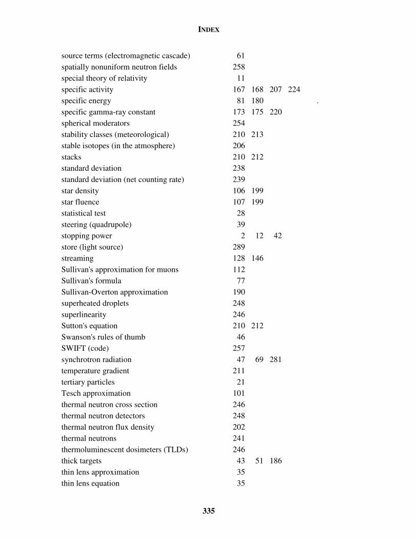
INDEX
335
source terms (electromagnetic cascade) 61 spatially nonuniform neutron fields 258 special theory of relativity 11 specific activity 167 168 207 224 specific energy 81 180 . specific gamma-ray constant 173 175 220 spherical moderators 254 stability classes (meteorological) 210 213 stable isotopes (in the atmosphere) 206 stacks 210 212 standard deviation 238 standard deviation (net counting rate) 239 star density 106 199 star fluence 107 199 statistical test 28 steering (quadrupole) 39 stopping power 2 12 42 store (light source) 289 streaming 128 146 Sullivan's approximation for muons 112 Sullivan's formula 77 Sullivan-Overton approximation 190 superheated droplets 248 superlinearity 246 Sutton's equation 210 212 Swanson's rules of thumb 46 SWIFT (code) 257 synchrotron radiation 47 69 281 temperature gradient 211 tertiary particles 21 Tesch approximation 101 thermal neutron cross section 246 thermal neutron detectors 248 thermal neutron flux density 202 thermal neutrons 241 thermoluminescent dosimeters (TLDs) 246 thick targets 43 51 186 thin lens approximation 35 thin lens equation 35
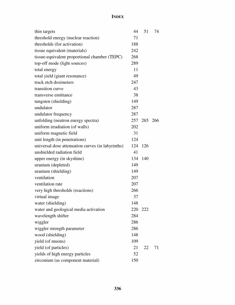
INDEX
336
thin targets 44 51 74 threshold energy (nuclear reaction) 71 thresholds (for activation) 188 tissue equivalent (materials) 242 tissue-equivalent proportional chamber (TEPC) 268 top-off mode (light sources) 289 total energy 11 total yield (giant resonance) 49 track etch dosimeters 247 transition curve 43 transverse emittance 38 tungsten (shielding) 149 undulator 287 undulator frequency 287 unfolding (neutron energy spectra) 257 265 266 uniform irradiation (of walls) 202 uniform magnetic field 31 unit length (in penetrations) 124 universal dose attenuation curves (in labyrinths) 124 126 unshielded radiation field 41 upper energy (in skyshine) 134 140 uranium (depleted) 149 uranium (shielding) 149 ventilation 207 ventilation rate 207 very high thresholds (reactions) 266 virtual image 37 water (shielding) 148 water and geological media activation 220 222 wavelength shifter 284 wiggler 286 wiggler strength parameter 286 wood (shielding) 148 yield (of muons) 109 yield (of particles) 21 22 71 yields of high energy particles 52 zirconium (as component material) 150