Embed Size (px)
Citation preview

Radio-frequency Linear Accelerators
437
14
Radio-Frequency Linear Accelerators
Resonant linear accelerators are usually single-pass machines. Charged particles traverse eachsection only once; therefore, the kinetic energy of the beam is limited by the length of theaccelerator. Strong accelerating electric fields are desirable to achieve the maximum kineticenergy in the shortest length. Although linear accelerators cannot achieve beam, output energy ashigh as circular accelerators, the following advantages dictate their use in a variety of applications:(1) the open geometry makes it easier to inject and extract beams; (2) high-flux beams can betransported because of the increased options for beam handling and high-power rf structures; and(3) the duty cycle is high. The duty cycle is defined as the fraction of time that the machineproduces beam output.
The operation of resonant linear accelerators is based on electromagnetic oscillations in tunedstructures. The structures support a traveling wave component with phase velocity close to thevelocity of accelerated particles. The technology for generating the waves and the interactionsbetween waves and particles were described in Chapters 12 and 13. Although the term radio

Radio-frequency Linear Accelerators
438
frequency (rf) is usually applied to resonant accelerators, it is somewhat misleading. Althoughsome resonant linear accelerators have been constructed with very large or inductive structures,most present accelerators use resonant cavities or waveguides with dimensions less than 1 m tocontain electromagnetic oscillations; they operate in the microwave regime (> 300 MHz).
Linear accelerators are used to generate singly-charged light ion beams in the range of 10 to300 MeV or multiply charged heavy ions up to 4 GeV (17 MeV/nucleon). These acceleratorshave direct applications such as radiation therapy, nuclear research, production of short-livedisotopes, meson production, materials testing, nuclear fuel breeding, and defense technology. Ionlinear accelerators are often used as injectors to form high-energy input beams for large circularaccelerators. The recent development of the radio-frequency quadrupole (RFQ), which is effectivefor low-energy ions, suggests new applications in the 1-10 MeV range, such as high-energy ionimplantation in materials. Linear accelerators for electrons are important tools for high-energyphysics research because they circumvent the problems of synchrotron radiation thatlimit beamenergy in circular accelerators. Electron linear accelerators are also used as injectors for circularaccelerators and storage rings. Applications for high-energy electrons include the generation ofsynchrotron radiation for materials research and photon beam generation through the free electronlaser process.
Linear accelerators for electrons differ greatly in both physical properties and technologicalrealization from ion accelerators. The contrasts arise partly from dissimilar applicationrequirements and partly from the physical properties of the particles. Ions are invariably non-relativistic; therefore, their velocity changes significantly during acceleration. Resonant linearaccelerators for ions are complex machines, often consisting of three or four different types ofacceleration units. In contrast, high-gradient electron accelerators for particle physics researchhave a uniform structure throughout their length. These devices are described in Section 14.1.Electrons are relativistic immediately after injection and have constant velocity through theaccelerator. Linear electron accelerators utilize electron capture by strong electric fields of a wavetraveling at the velocity of light. Because of the large power dissipation, the machines areoperated in a pulsed mode with low-duty cycle. After a description of the general properties ofthe accelerators, Section 14.1 discusses electron injection, beam breakup instabilities, the designof iris-loaded wave-guides withω/k = c, optimization of power distribution for maximum kineticenergy, and the concept of shunt impedance.
Sections 14.2-14.4 review properties of high-energy linear ion accelerators. The four commonconfigurations of rf ion accelerators are discussed in Sections 14.2 and 14.3: the Wideröeaccelerator, the independently-phased cavity array, the drift tube linac, and the coupled cavityarray. Starting from the basic Wideröe geometry, the rationale for surrounding acceleration gapswith resonant structures is discussed. The configuration of the drift tube linac is derivedqualitatively by considering an evolutionary sequence from the Wideröe device. The principles ofcoupled cavity oscillations are discussed in Section 14.3. Although a coupled cavity array is moredifficult to fabricate than a drift tube linac section, the configuration has a number of benefits forhigh-flux ion beams when operated in a particular mode (theπ/2 mode). Coupled cavities havehigh accelerating gradient, good frequency stability, and strong energy coupling. The latterproperty is essential for stable electromagnetic oscillations in the presence of significant beam

Radio-frequency Linear Accelerators
439
loading. Examples of high-energy ion accelerators are included toillustrate strategies forcombining the different types of acceleration units into a high-energy system.
Some factors affecting ion transport in rf linacs are discussed in Section 14.4. Included are thetransit-time factor, gap coefficients, and radial defocusing by rf fields. The transit-time factor isimportant when the time for a particle to cross an acceleration gap is comparable to half the rfperiod. In this case, the peak energy gain (reflecting the integral of charge times electric fieldduring the transit) is less than the product of charge and peak gap voltage. The transit-timederating factor must be included to determine the synchronous particle orbit. The gap coefficientrefers to radial variations of longitudinal electric field. The degree of variation depends on the gapgeometry and rf frequency. The spatial dependence ofEz leads to increased energy spread inthe output beam or reduced longitudinal acceptance. Section 14.4 concludes with a discussion ofthe effects of the radial fields of a slow traveling wave on beam containment. The existence andnature of radial fields are derived by a transformation to the rest frame of the wave in it appears aselectrostatic field pattern. The result is that orbits in cylindrically symmetric rf linacs are radiallyunstable if the particles are in a phase region of longitudinal stability. Ion linacs must thereforeincorporate additional focusing elements (such as an FD quadrupole array) to ensure containmentof the beam.
Problems of vacuum breakdown in high-gradient rf accelerators are discussed in Section 14.5.The main difference from the discussion of Section 9.5 is the possibility for geometric growth ofthe number of secondary electrons emitted from metal surfaces when the electron motion is insynchronism with the oscillating electric fields. This process is called multipactoring. Electronmultipactoring is sometimes a significant problem in starting up rf cavities; ultimate limits onaccelerating gradient in rf accelerators may be set by ion multipactoring.
Section 14.6 describes the RFQ, a recently-developed configuration. The RFQ differs almostcompletely from other rf linac structures. The fields are azimuthally asymmetric and the mainmode of excitation of the resonant structure is a TE mode rather than a TM mode. The RFQ hassignificant advantages for the acceleration of high-flux ion beams in the difficult low-energyregime (0.1-5 MeV). The structure utilizes purely electrostatic focusing from rf fields to achievesimultaneous average transverse and longitudinal containment. The electrode geometries in thedevice can be fabricated to generate precise field variations over small-scale lengths. This givesthe RFQ the capability to perform beam bunching within theaccelerator, eliminating the need fora separate buncher and beam transport system. At first glance, the RFQ appears to be difficult todescribe theoretically. In reality, the problem is tractable if we divide it into parts and applymaterial from previous chapters. The properties of longitudinally uniform RFQs, such as theinterdependence of accelerating gradient and transverse acceptance and the design of shapedelectrodes, can be derived with little mathematics.
Section 14.7 reviews the racetrack microtron, an accelerator with the ability to producecontinuous high-energy electron beams. The racetrack microtron is a hybrid between linear andcircular accelerators; it is best classified as a recirculating resonant linear accelerator. The machineconsists of a short linac (with a traveling wave component withω/k = c) and two regions ofuniform magnetic field. The magnetic fields direct electrons back to the entrance of theaccelerator in synchronism with the rf oscillations. Energy groups of electrons follow separate
Radio-frequency Linear Accelerators
440
orbits which require individual focusing and orbit correction elements. Synchrotron radiationlimits the beam kinetic energy of microtrons to less than 1 GeV. Beam breakup instabilities are amajor problem in microtrons; therefore, the output beam current is low (< 100 µA). Nonetheless,the high-duty cycle of microtrons means that the time-averaged electron flux is much greater thanthat from conventional electron linacs.
14.1 ELECTRON LINEAR ACCELERATORS
Radio-frequency linear accelerators are used to generate high-energy electron beams in the rangeof 2 to 20 GeV. Circular election accelerators cannot reach high output kinetic energy because ofthe limits imposed by synchrotron radiation. Linearaccelerators for electrons are quite differentfrom ion accelerators. They are high-gradient, traveling wave structures used primarily for particlephysics research. Accelerating gradient is the main figure of merit; consequently, the efficiencyand duty cycle of electron linacs are low. Other accelerator configurations are used when a hightime-averaged flux of electrons at moderate energy is required. One alternative, the racetrackmicrotron, is described in Section 14.7.
A. General Properties
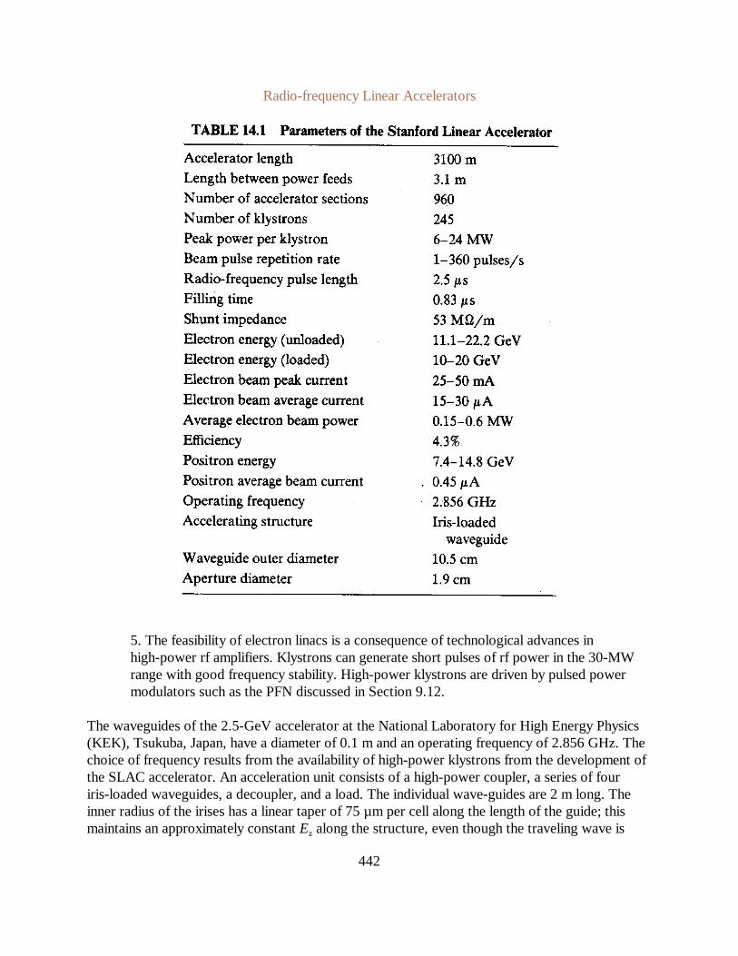
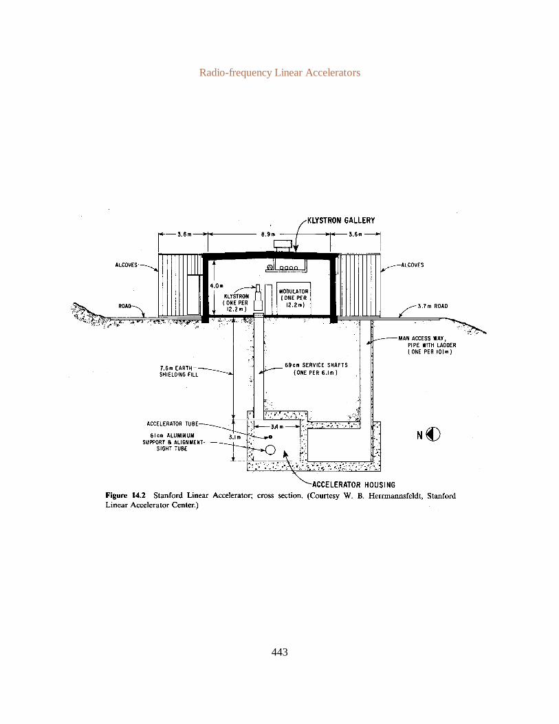
Figure 14.1 shows a block diagram of an electron linac. The accelerator typically consists of asequence of identical, iris-loaded slow-wavestructures that support traveling waves. Thewaveguides are driven by high-power klystron microwave amplifiers. The axial electric fields ofthe waves are high, typically on the order of 8 MV/m. Parameters of the 20-GeV acceleratorat the Stanford Linear Accelerator Center are listed in Table 14.1. The accelerator is over 3 km inlength; the open aperture for beam transport is only 2 cm in diameter. The successful transport ofthe beam through such a long, narrow tube is a consequence of the relativistic contraction of theapparent length of the accelerator (Section 13.6). A cross section of the accelerator isillustratedin Figure 14.2. A scale drawing of the rf power distribution system is shown in Figure 14.3.
The features of high-energy electron linear accelerators are determined by the followingconsiderations.
1. Two factors motivate the use of strong accelerating electric fields: (a) high gradient isfavorable for electron capture (Section 13.6) and (b) the accelerator length for a givenfinal beam energy is minimized.
2. Resistive losses per unit length are large in a high-gradient accelerator because powerdissipation in the waveguide walls scales asEz
2. Dissipation is typically greater than 1MW/m. Electron linacs must be operated on an intermittent duty cycle with a beampulselength of a few microseconds.

Radio-frequency Linear Accelerators
441
3. An iris-loaded waveguide with relatively large aperture can support slow waves withω/k = c. Conduction of rf energy along the waveguide is effective; nonetheless, the wavesare attenuated because of the high losses. There is little to be gained by reflecting thetraveling waves to produce a standing wave pattern. In practice, the energy of theattenuated wave is extracted from the waveguide at the end of an accelerating section anddeposited in an external load. This reduces heating of the waveguides.
4. A pulsed electron beam is injected after the waveguides are filled with rf energy. Thebeam pulse length is limited by theaccelerator duty cycle and by the growth of beambreakup instabilities. Relatively high currents (0.1 A) are injected to maximize thenumber of electrons available for experiments.
Radio-frequency Linear Accelerators
442
5. The feasibility of electron linacs is a consequence of technological advances inhigh-power rf amplifiers. Klystrons can generate short pulses of rf power in the 30-MWrange with good frequency stability. High-power klystrons are driven by pulsed powermodulators such as the PFN discussed in Section 9.12.
The waveguides of the 2.5-GeV accelerator at the National Laboratory for High Energy Physics(KEK), Tsukuba, Japan, have a diameter of 0.1 m and an operating frequency of 2.856 GHz. Thechoice of frequency results from the availability of high-power klystrons from the development ofthe SLAC accelerator. An acceleration unit consists of a high-power coupler, a series of fouriris-loaded waveguides, a decoupler, and a load. The individual wave-guides are 2 m long. Theinner radius of the irises has a linear taper of 75 µm per cell along the length of the guide; thismaintains an approximately constantEz along the structure, even though the traveling wave is
Radio-frequency Linear Accelerators
443

Radio-frequency Linear Accelerators
444
attenuated. Individual waveguides of a unit have the same phase velocity but vary in therelative dimensions of the wall and iris to compensate for their differing distance from the rfpower input. There are five types of guides in the accelerator; the unit structure is varied tominimize propagation of beam-excited modes which could contribute to the beam breakupinstability. Construction of the guides utilized modern methods of electroplating and precisionmachining. A dimensional accuracy of ± 2 µm and a surface roughness of 200 was achieved,making postfabrication tuning unnecessary.
Radio-frequency Linear Accelerators
445
B. Injection
The pulsed electron injector of a high-power electron linear accelerator is designed for highvoltage (> 200 kV) to help in electron capture. The beam pulselength may vary from a fewnanoseconds to 1 µs depending on the research application. The high-current beam must be aimedwith a precision of a few milliradians to prevent beam excitation of undesired rf modes in theaccelerator. Before entering the accelerator, the beam is compressed into micropulses by abuncher. A buncher consists of an rf cavity or a short section of iris-loaded waveguide operatingat the same frequency as the main accelerator. Electrons emerge from the buncher cavity with alongitudinal velocity dispersion. Fast particles overtake slow particles, resulting in downstreamlocalization of the beam current to sharp spikes. The electrons must be confined within a smallspread in phase angle ( ) to minimize the kinetic energy spread of the output beam. 5
The micropulses enter the accelerator at a phase between 0 and 90. As we saw in Section13.6, the average phase of the pulse increases until the electrons are ultra-relativistic. For theremainder of the acceleration cycle, acceleration takes place near a constant phase called theasymptotic phase. The injection phase of the micropulses and the accelerating gradient areadjusted to give an asymptotic phase of 90. This choice gives the highest acceleration gradientand the smallest energy spread in the bunch.
Output beam energy uniformity is a concern for high-energy physics experiments. The outputenergy spread is affected by variations in the traveling wave phase velocity. Dimensionaltolerances in the waveguides on the order of 10-3 cm must be maintained for a 1% energy spread.The structures must be carefully machined and tuned. The temperature of the waveguides under rfpower loading must be precisely controlled to prevent a shift in phase velocity from thermalexpansion.
C. Beam Breakup Instability
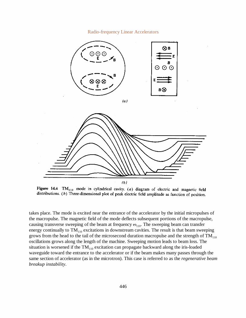
The theory of Section 13.6 indicated that transverse focusing is unnecessary in an electron linacbecause of the shortened effective length. This is true only at low beam current; at high current,electrons are subject to thebeam breakup instability[W. K. H. Panofsky and M. Bander, Rev.Sci. Instrum.39, 206 (1968); V. K. Neil and R. K. Cooper, Part. Accel.1, 111 (1970)] alsoknown as thetransverse instabilityor pulse shortening. The instability arises from excitation ofTM110 cavity modes in the spaces between irises. Features of the TM110 mode in a cylindricalcavity are illustrated in Figure 14.4. Note that there are longitudinal electric fields of oppositepolarity in the upper and lower portions of the cavity and that there is a transverse magnetic fieldon the axis. An electron micropulse (of sub-nanosecond duration) can be resolved into a broadspectrum of frequencies. If the pulse has relatively high current and is eccentric with respect to thecavity, interaction between the electrons and the longitudinal electric field of the TM110 mode
Radio-frequency Linear Accelerators
446
takes place. The mode is excited near the entrance of the accelerator by the initial micropulses ofthe macropulse. The magnetic field of the mode deflects subsequent portions of the macropulse,causing transverse sweeping of the beam at frequencyω110. The sweeping beam can transferenergy continually to TM110 excitations in downstream cavities. The result is that beam sweepinggrows from the head to the tail of the microsecond duration macropulse and the strength of TM110
oscillations grows along the length of the machine. Sweeping motion leads to beam loss. Thesituation is worsened if the TM110 excitation can propagate backward along the iris-loadedwaveguide toward the entrance to the accelerator or if the beam makes many passes through thesame section of accelerator (as in the microtron). This case is referred to as theregenerative beambreakup instability.

Radio-frequency Linear Accelerators
447
Ez(standing wave) 0 at r Ro, (14.1)
Ez(traveling wave) Ez(standing wave) at r R, (14.2)
Bθ(traveling wave) B
θ(standing wave) at r R. (14.3)
The beam breakup instability has the following features.
1. Growth of the instability is reduced byaccurate injection of azimuthally symmetricbeams.
2. The energy available to excite undesired modes is proportional to the beam current.Instabilities are not observed below a certain current; the cutoff depends on themacropulselength and the Q values of the resonant structure.
3. The amplitude of undesired modes grows with distance along the accelerator and withtime. This explains pulse shortening, the loss of late portions of the electron macropulse.
4. Mode growth is reduced by varying the accelerator structure. The phase velocity forTM01 traveling waves is maintained constant, but the resonant frequency for TM110
standing waves between irises is changed periodically along the accelerator.
Transverse focusing elements are necessary in high-energy electron linear accelerators tocounteract the transverse energy gained through instabilities. Focusing is performed by solenoidlenses around the waveguides or by magnetic quadrupole lenses between guide sections.
D. Frequency Equation
The dispersion relationship for traveling waves in an iris-loaded waveguide was introduced inSection 12-10. We shall determine the approximate relationship between the inner and outer radiiof the irises for waves with phase velocityω/k = c at a specified frequency. Thefrequencyequationis a first-order guide. A second-order waveguide design is performed with computercalculations and modeling experiments.
Assume thatδ, the spacing between irises, is small compared to the wavelength of the travelingwave; the boundary fields approximate a continuous function. The tube radius isRo and theaperture radius isR. The complete solution consists of standing waves in the volume between theirises and a traveling wave matched to the reactive boundary atr = Ro. The solution mustsatisfy the following boundary conditions:
The last two conditions proceed from the fact thatE andB must be continuous in the absence ofsurface charges or currents.
Radio-frequency Linear Accelerators
448
Ez(r,t) A J0(ωr/c) B Y0(ωr/c). (14.4)
Ez Eo [Y0(ωRo/c) J0(ωr/c) J0(ωRo/c) Y0(ωr/c)]. (14.5)
Bθ (jEo/c) [Y0(ωRo/c) J1(ωr/c) J0(ωRo/c) Y1(ωr/c)]. (14.6)
Id πR2 (Ez/t)/µoc2 (jω/µoc
2) (πR2) Eo exp[j(kzωt)]. (14.7)
Bθ (jωR/2c2) Eo exp[j(kzωt)]. (14.8)
ωR/c
2 [Y0(ωRo/c) J1(ωR/c) J0(ωRo/c) Y1(ωR/c)]
Y0(ωRo/c) J0(ωR/c) J0(ωRo/c) Y0(ωR/c). (14.9)
Following Section 12.3, the solution for azimuthally symmetric standing waves in the spacebetween the irises is
T'he Y0 term is retained because the region does not include the axis. Applying Eq. (14.1), Eq.(14.4) becomes
The toroidal magnetic field is determined from Eq. (12.45) as
The traveling wave has an electric field of the form .We shall see inEz Eo exp[j(kzωt)]Section 14.4 that the axial electric field of the traveling wave is approximately constant over theaperture. Therefore, the net displacement current carried by a wave with phase velocity equal tocis
The toroidal magnetic field of the wave atr = R is
The frequency equation is determined by setting for the cavities and for the traveling waveEz/Bθ
equal atr = R [Eqs. (14.2) and (14.3)1:
Equation (14.9) is a transcendental equation that determinesω in terms ofR andRo to generate atraveling wave with phase velocity equal to the speed of light. A plot of the right-hand side of theequation is given in Figure 14.5. A detailed analysis shows that power flow is maximized andlosses minimized when there are about four irises per wavelength. Although the assumptionsunderlying Eq. (14.9) are not well satisfied in this limit, it still provides a good first-orderestimate.

Radio-frequency Linear Accelerators
449
(dP/dz) Uω/Q. (14.10)
vg energy flux
electromagnetic energy density.
E. Electromagnetic Energy Flow
Radio-frequency power is inserted into the waveguides periodically at locations separated by adistancel. For a given available total powerP, and accelerator lengthL, we can show that there isan optimum value ofl such that the final beam energy is maximized. In analogy with standingwave cavities, the quantityQ characterizes resistive energy loss in the waveguide according to
In Eq, (14.10), dP/dz is the power lost per unit length along the slow-wave structure andU is theelectromagnetic energy per unit length. Following the discussion of Section 12.10, the groupvelocity of the traveling waves is equal to
Multiplying the numerator and denominator by the area of the waveguide implies

Radio-frequency Linear Accelerators
450
Uvg P, (14.11)
P(z) Po exp(ωz/Qvg), (14.12)
Ez(z) Ezo exp(z/lo), (14.13)
∆T e
l
0
Ez(z) dz. (14.14)
∆T eEzol [1 exp(l/l o)] / (l/lo). (14.15)
Pt (vgE2zo) (L/l),
whereP is the total power flow. Combining Eqs. (14.10) and (14.11), ,or (dP/dz) (ω/Qvg) P
wherePo is the power input to a waveguide section atz = 0. The electromagnetic power flow isproportional to the Poynting vector whereEz is the magnitude of the peakS E ×H E 2
z
axial electric field. We conclude that electric field as a function of distance from the power input isdescribed by
where .An electron traveling through an accelerating section of lengthl gains anlo 2Qvg/ωenergy
Substituting from Eq. (14.13) gives
In order to find an optimum value ofl, we must define the following constraints:
1.The total rf powerPt and total accelerator lengthL are specified. The power input to anaccelerating section of length l is .∆P Pt (l/L)
2. The waveguide propertiesQ, vg, andω are specified.
The goal is to maximize the total energy by varying the number of power inputT ∆T (L/l)points. The total power scales as
where the first factor is proportional to the input power flux to a section and the second factor isthe number of sections. Therefore, with constant power,Ezo scales as . Substituting the scalinglfor Ezo in Eq. (14.15) and multiplying byL/l, we find that the beam output energy scales as
Radio-frequency Linear Accelerators
451
T l [1 exp(l/lo)]/l
T [1 exp(l/lo)] / l/lo. (14.16)
or
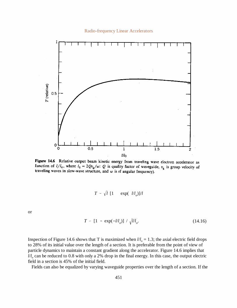
Inspection of Figure 14.6 shows that T is maximized whenl/lo = 1.3; the axial electric field dropsto 28% of its initial value over the length of a section. It is preferable from the point of view ofparticle dynamics to maintain a constant gradient along the accelerator. Figure 14.6 implies thatl/lo can be reduced to 0.8 with only a 2% drop in the final energy. In this case, the output electricfield in a section is 45% of the initial field.
Fields can also be equalized by varying waveguide properties over the length of a section. If the

Radio-frequency Linear Accelerators
452
Pt V2o / (ZsL), (14.17)
Zs E 2z / (dP/dz), (14.18)
energy efficiency Zb/(Zb ZsL), (14.19)
wall radius and the aperture radius are decreased consistent with Eq. (14.9), the phase velocity ismaintained atc while the axial electric field is raised for a given power flux. Waveguides can bedesigned for constant axial field in the presence of decreasing power flux. In practice, it is difficultto fabricate precision waveguides with continuously varying geometry. A common compromise isto divide an accelerator section into subsections with varying geometry. The sections must becarefully matched so that there is no phase discontinuity between them. This configuration has theadditional benefit of reducing the growth of beam breakup instabilities.
F. Shunt Impedance
Theshunt impedanceis a figure-of-merit quantity for electron and ion linear accelerators. It isdefined by
wherePt is the total power dissipated in the cavity walls of the accelerator,Vo is the totalaccelerator voltage (the beam energy in electron volts divided by the particle charge), andL is thetotal accelerator length. The shunt impedanceZs has dimensions of ohms per meter. An alternateform for shunt impedance is
where dP/dz is the resistive power loss per meter. The power loss of Eq. (14.17) has the form of aresistor of valueZsL in parallel with the beam load. This is the origin of the term shunt impedance.
The efficiency of a linear accelerator is given by
whereZb is the beam impedance, . The shunt impedance for most accelerator rfZb Vo/i bstructures lies in the range of 25 to 50 MΩ/m. As an example, consider a 2.5-GeV linear electronaccelerator with a peak on-axis gradient of 8 MV/m. The total accelerator length is 312 m. With ashunt impedance of 50 MΩ/m, the total parallel resistance is 1.6 x 10¹⁰ Ω. Equation (14.17)implies that the power to maintain the high acceleration gradient is 400 MW.
14.2 LINEAR ION ACCELERATOR CONFIGURATIONS
Linear accelerators for ions differ greatly from electron machines. Ion accelerators must support
Radio-frequency Linear Accelerators
453
traveling wave components with phase velocity well below the speed of light. In the energy rangeaccessible to linear accelerators, ions are non-relativistic; therefore, there is a considerable changein the synchronous particle velocity during acceleration. Slow-wave structures are not useful forion acceleration. An iris-loaded waveguide has small apertures for . The conduction ofω/k « celectromagnetic energy via slow waves is too small to drive a multi-cavity waveguide. Alternativemethods of energy coupling are used to generate traveling wave components with slow phasevelocity.
An ion linear accelerator typically consists of a sequence of cylindrical cavities supportingstanding waves. Cavity oscillations are supported either by individual power feeds or throughinter-cavity coupling via magnetic fields. The theory of ion accelerators is most effectively carriedout by treating cavities as individual oscillators interacting through small coupling terms.
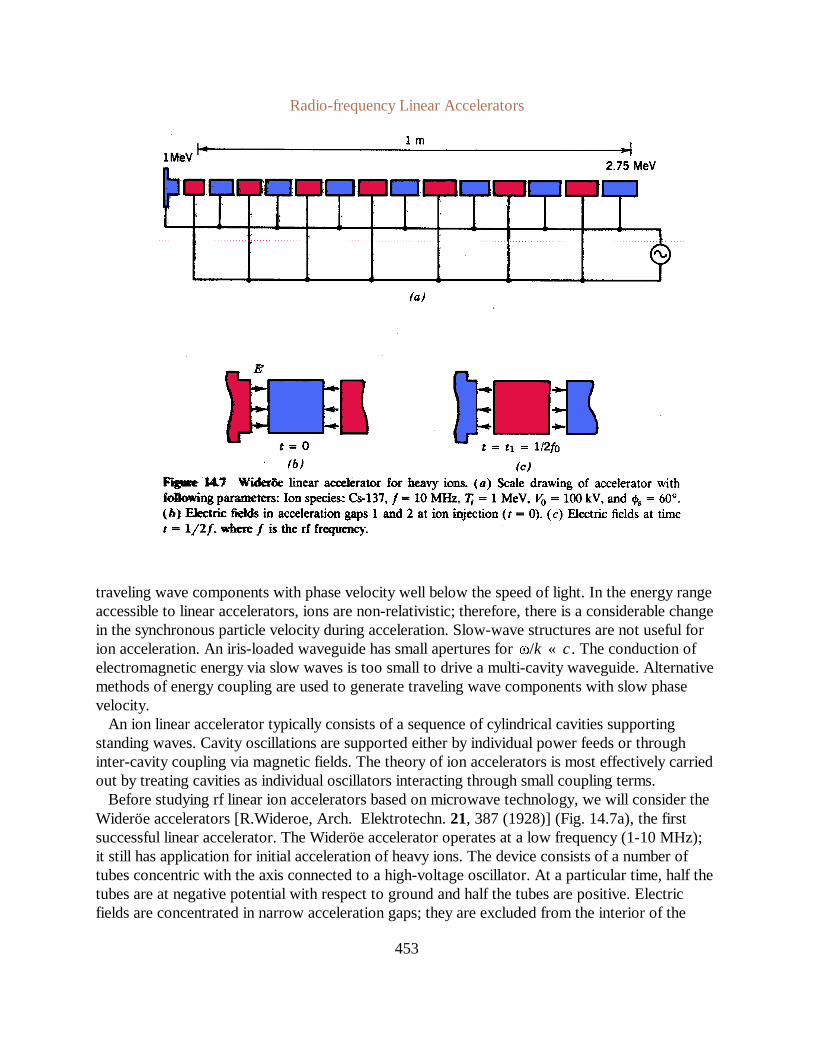
Before studying rf linear ion accelerators based on microwave technology, we will consider theWideröe accelerators [R.Wideroe, Arch. Elektrotechn.21, 387 (1928)] (Fig. 14.7a), the firstsuccessful linear accelerator. The Wideröe accelerator operates at a low frequency (1-10 MHz);it still has application for initial acceleration of heavy ions. The device consists of a number oftubes concentric with the axis connected to a high-voltage oscillator. At a particular time, half thetubes are at negative potential with respect to ground and half the tubes are positive. Electricfields are concentrated in narrow acceleration gaps; they are excluded from the interior of the

Radio-frequency Linear Accelerators
454
∆t1 L1/vs1. (14.20)
∆t1 π/ω. (14.21)
V1 (LCcω2o) V2 (1 LCω2
LCcω2o) 0. (14.22)
Ln vn (π/ω). (14.23)
tubes. The tubes are referred to asdrift tubesbecause ions drift at constant velocity inside theshielded volume. Assume that the synchronous ion crosses the first gap at t = 0 when the fieldsare aligned as shown in Figure 14.7b. The ion is accelerated across the gap and enters thezero-field region in the first drift tube. The ion reaches the second gap at time
The axial electric fields att = t1 are distributed as shown in Figure 14.7c ift1 is equal to half the rfperiod, or
The particle is accelerated in the second gap when Eq. (14.21) holds.It is possible to define a synchronous orbit with continuous acceleration by increasing the length
of subsequent drift tubes. The velocity of synchronous ions following thenth gap is
hereTo is the injection kinetic energy,Vo is the peak gap voltage, andφs is the synchronousphase. The length of drift tuben is
The drift tubes of Figure 14.7a are drawn to scale for the acceleration of Hg+ ions injected at 2MeV with a peak gap voltage of 100 kV and a frequency of 4 MHz.
The Wideröe accelerator is not useful for light-ion acceleration and cannot be extrapolated toproduce high-energy heavy ions. At high energy, the drift tubes are unacceptably long, resulting ina low average accelerating gradient. The drift tube length is reduced if the rf frequency isincreased, but this leads to the following problems:
1.The acceleration gaps conduct large displacement currents at high frequency, loading therf generator.
2.Adjacent drift tubes act as dipole antennae at high frequency with attendant loss of rfenergy by radiation.
The high-frequency problems are solved if the acceleration gap is enclosed in a cavity withresonant frequencyω. The cavity walls reflect the radiation to produce a standing electromagneticoscillation. The cavity inductance in combination with the cavity and gap capacitance constituteanLC circuit. Displacement currents are supported by the electromagnetic oscillations. Thepower supply need only contribute energy to compensate for resistive losses and beam loading.

Radio-frequency Linear Accelerators
455
A resonant cavity for ion acceleration is shown in Figure 14.8a. The TM010 mode producesgood electric fields for acceleration. We have studied the simple cylindrical cavity in Section 12.3.The addition of drift tube extensions to the cylindrical cavity increases the capacitance on axis,thereby lowering the resonant frequency. The resonant frequency can be determined by aperturbation analysis or through the use of computer codes. The electric field distribution for alinac cavity computed by the program SUPERFISH is shown in Figure 14.8b.
Linear ion accelerators are composed of an array of resonant cavities. We discussed thesynthesis of slow waves by independently phased cavities in Section 12.9. Two frequently
Radio-frequency Linear Accelerators
456
Ln vn (2π/ω) βλ, (14.24)
Ln βλ/2. (14.25)
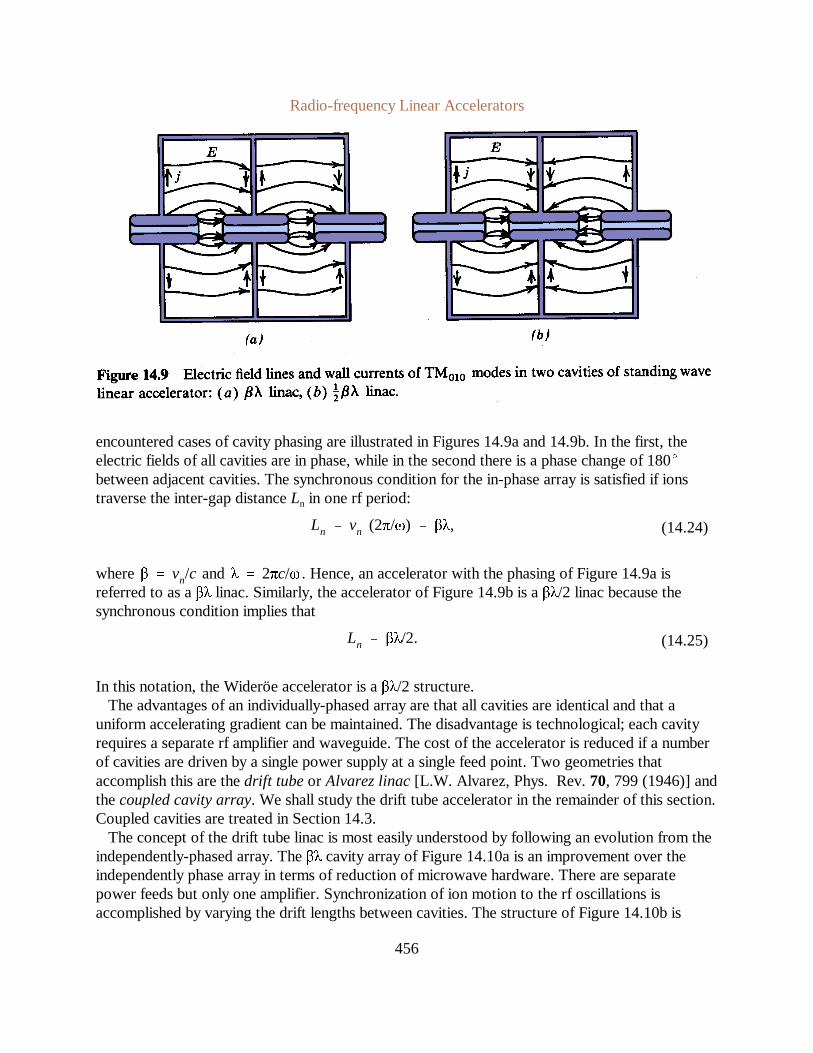
encountered cases of cavity phasing are illustrated in Figures 14.9a and 14.9b. In the first, theelectric fields of all cavities are in phase, while in the second there is a phase change of 180
between adjacent cavities. The synchronous condition for the in-phase array is satisfied if ionstraverse the inter-gap distanceLn in one rf period:
where and . Hence, an accelerator with the phasing of Figure 14.9a isβ vn/c λ 2πc/ωreferred to as aβλ linac. Similarly, theaccelerator of Figure 14.9b is aβλ/2 linac because thesynchronous condition implies that
In this notation, the Wideröe accelerator is aβλ/2 structure.The advantages of an individually-phased array are that all cavities are identical and that a
uniform accelerating gradient can be maintained. The disadvantage is technological; each cavityrequires a separate rf amplifier and waveguide. The cost of the accelerator is reduced if a numberof cavities are driven by a single power supply at a single feed point. Two geometries thataccomplish this are thedrift tubeor Alvarez linac[L.W. Alvarez, Phys. Rev.70, 799 (1946)] andthecoupled cavity array. We shall study the drift tube accelerator in the remainder of this section.Coupled cavities are treated in Section 14.3.
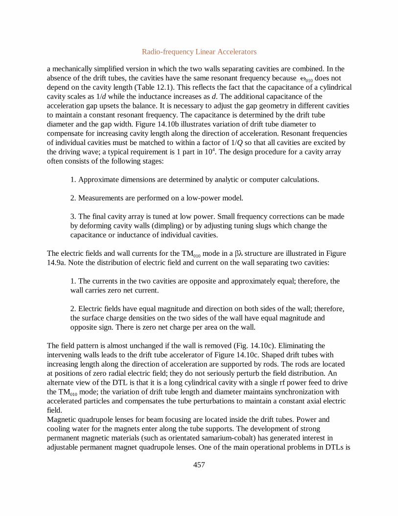
The concept of the drift tube linac is most easily understood by following an evolution from theindependently-phased array. Theβλ cavity array of Figure 14.10a is an improvement over theindependently phase array in terms of reduction of microwave hardware. There are separatepower feeds but only one amplifier. Synchronization of ion motion to the rf oscillations isaccomplished by varying the drift lengths between cavities. The structure of Figure 14.10b is
Radio-frequency Linear Accelerators
457
a mechanically simplified version in which the two walls separating cavities are combined. In theabsence of the drift tubes, the cavities have the same resonant frequency becauseω010 does notdepend on the cavity length (Table 12.1). This reflects the fact that the capacitance of a cylindricalcavity scales as 1/d while the inductance increases asd. The additional capacitance of theacceleration gap upsets the balance. It is necessary to adjust the gap geometry in different cavitiesto maintain a constant resonant frequency. The capacitance is determined by the drift tubediameter and the gap width. Figure 14.10b illustrates variation of drift tube diameter tocompensate for increasing cavity length along the direction of acceleration. Resonant frequenciesof individual cavities must be matched to within a factor of 1/Q so that all cavities are excited bythe driving wave; a typical requirement is 1 part in 104. The design procedure for a cavity arrayoften consists of the following stages:
1. Approximate dimensions are determined by analytic or computer calculations.
2. Measurements are performed on a low-power model.
3. The final cavity array is tuned at low power. Small frequency corrections can be madeby deforming cavity walls (dimpling) or by adjusting tuning slugs which change thecapacitance or inductance of individual cavities.
The electric fields and wall currents for the TM010 mode in aβλ structure are illustrated in Figure14.9a. Note the distribution of electric field and current on the wall separating two cavities:
1. The currents in the two cavities are opposite and approximately equal; therefore, thewall carries zero net current.
2. Electric fields have equal magnitude and direction on both sides of the wall; therefore,the surface charge densities on the two sides of the wall have equal magnitude andopposite sign. There is zero net charge per area on the wall.
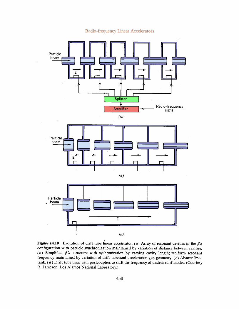
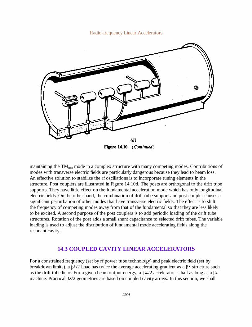
The field pattern is almost unchanged if the wall is removed (Fig. 14.10c). Eliminating theintervening walls leads to the drift tube accelerator of Figure 14.10c. Shaped drift tubes withincreasing length along the direction of acceleration are supported by rods. The rods are locatedat positions of zero radial electric field; they do not seriously perturb the field distribution. Analternate view of the DTL is that it is a long cylindrical cavity with a single rf power feed to drivethe TM010 mode; the variation of drift tube length and diameter maintains synchronization withaccelerated particles and compensates the tube perturbations to maintain a constant axial electricfield.Magnetic quadrupole lenses for beam focusing are located inside the drift tubes. Power andcooling water for the magnets enter along the tube supports. The development of strongpermanent magnetic materials (such as orientated samarium-cobalt) has generated interest inadjustable permanent magnet quadrupole lenses. One of the main operational problems in DTLs is
Radio-frequency Linear Accelerators
458
Radio-frequency Linear Accelerators
459
maintaining the TM010 mode in a complex structure with many competing modes. Contributions ofmodes with transverse electric fields are particularly dangerous because they lead to beam loss.An effective solution to stabilize the rf oscillations is to incorporate tuning elements in thestructure. Post couplers are illustrated in Figure 14.10d. The posts are orthogonal to the drift tubesupports. They have little effect on the fundamental acceleration mode which has only longitudinalelectric fields. On the other hand, the combination of drift tube support and post coupler causes asignificant perturbation of other modes that have transverse electric fields. The effect is to shiftthe frequency of competing modes away from that of the fundamental so that they are less likelyto be excited. A second purpose of the post couplers is to add periodic loading of the drift tubestructures. Rotation of the post adds a small shunt capacitance to selected drift tubes. The variableloading is used to adjust the distribution of fundamental mode accelerating fields along theresonant cavity.
14.3 COUPLED CAVITY LINEAR ACCELERATORS
For a constrained frequency (set by rf power tube technology) and peak electric field (set bybreakdown limits), aβλ/2 linac has twice the average accelerating gradient as aβλ structure suchas the drift tube linac. For a given beam output energy, aβλ/2 accelerator is half as long as aβλmachine. Practicalβλ/2 geometries are based on coupled cavity arrays. In this section, we shall

Radio-frequency Linear Accelerators
460
C(dV1/dt) I1, (14.26)
V1 L (dI1/dt di/dt), (14.27)
C(dV2/dt) I2, (14.28)
V2 L (dI2/dt di/dt), (14.29)
i Cc (dV1/dt dV2/dt) (Cc/C) (I1 I2). (14.30)
i (Cc ω2o) (V1 V2). (14.31)
V1 (1 LCω2 LCcω
2o) V2 (LCcω
2o) 0, (14.32)
V1 (LCcω2o) V2 (1 LCω2
LCcω2o) 0. (14.33)
1Ω2κ κ
κ 1Ω2κ
V1
V2
0. (14.34)
analyze the coupled cavity formalism and study some practical configurations.To begin, we treat two cylindrical resonant cavities connected by a coupling hole (Fig. 14.11a).
The cavities oscillate in the TM010 mode. Each cavity can be represented as a lumped elementLCcircuit with (Fig. 14.11b). Coupling of modes through an on-axis hole is capacitive.ωo 1/ LCThe electric field of one cavity makes a small contribution to displacement current in the other(Fig. 14.11c). In the circuit model we can represent the coupling by a capacitorCc between thetwo oscillator circuits (Fig. 14.llb). If coupling is weak, . Similarly, an azimuthal slot nearCc « Cthe outer diameter of the wall between the cavities results in magnetic coupling. Some of thetoroidal magnetic field of one cavity leaks into the other cavity, driving wall currents throughinductive coupling (Fig. 14.11d). In the circuit model, a magnetic coupling slot is represented by amutual inductance (Fig. 14.11e).
The following equations describe voltage and current in the circuit of Figure 14.11b:
When coupling is small, voltages and currents oscillate at frequency to and the quantityiω ωois much smaller thanI1 or I2. In this case, Eq. (14.30) has the approximate form
Assuming solutions of the form , Eqs. (14.26)-(14.31) can be combined to giveV1,V2 exp(jωt)
Substituting and , Eqs. (14.32) and (14.33) can be written in matrix form:Ω ω/ωo κ Cc/C

Radio-frequency Linear Accelerators
461
Radio-frequency Linear Accelerators
462
(1Ω2κ2) κ2
0 (14.35)
Ω1 ω1/ωo 12κ, (14.36)
Ω2 ω2/ωo 1. (14.37)
The equations have a nonzero solution if the determinant of the matrix equals zero, or
Equation (14.35) has two solutions for the resonant frequency:
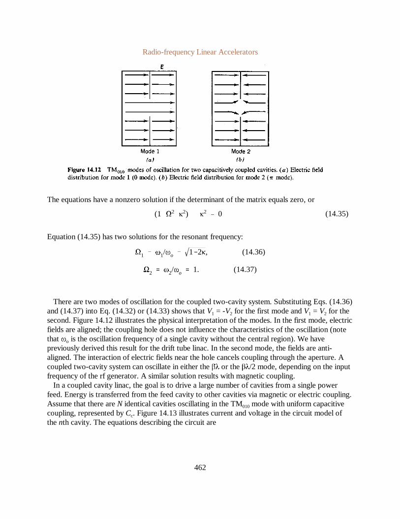
There are two modes of oscillation for the coupled two-cavity system. Substituting Eqs. (14.36)and (14.37) into Eq. (14.32) or (14.33) shows thatV1 = -V2 for the first mode andV1 = V2 for thesecond. Figure 14.12 illustrates the physical interpretation of the modes. In the first mode, electricfields are aligned; the coupling hole does not influence the characteristics of the oscillation (notethatωo is the oscillation frequency of a single cavity without the central region). We havepreviously derived this result for the drift tube linac. In the second mode, the fields are anti-aligned. The interaction of electric fields near the hole cancels coupling through the aperture. Acoupled two-cavity system can oscillate in either theβλ or theβλ/2 mode, depending on the inputfrequency of the rf generator. A similar solution results with magnetic coupling.
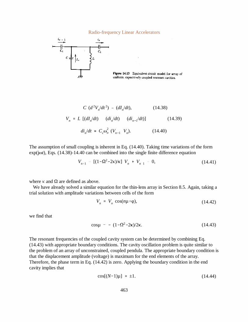
In a coupled cavity linac, the goal is to drive a large number of cavities from a single powerfeed. Energy is transferred from the feed cavity to other cavities via magnetic or electric coupling.Assume that there areN identical cavities oscillating in the TM010 mode with uniform capacitivecoupling, represented byCc. Figure 14.13 illustrates current and voltage in the circuit model ofthenth cavity. The equations describing the circuit are
Radio-frequency Linear Accelerators
463
C (d 2Vn/dt 2) (dIn/dt), (14.38)
Vn L [(dIn/dt) (din/dt) (din1/dt)] (14.39)
din/dt Ccω2o (Vn1Vn). (14.40)
Vn1 [(1Ω22κ)/κ] Vn Vn1 0, (14.41)
Vn Vo cos(nµφ), (14.42)
cosµ (1Ω22κ)/2κ. (14.43)
cos[(N1)µ] ±1. (14.44)
The assumption of small coupling is inherent in Eq. (14.40). Taking time variations of the formexp(jωt), Eqs. (14.38)-14.40 can be combined into the single finite difference equation
whereκ andΩ are defined as above.We have already solved a similar equation for the thin-lens array in Section 8.5. Again, taking a
trial solution with amplitude variations between cells of the form
we find that
The resonant frequencies of the coupled cavity system can be determined by combining Eq.(14.43) with appropriate boundary conditions. The cavity oscillation problem is quite similar tothe problem of an array of unconstrained, coupled pendula. The appropriate boundary condition isthat the displacement amplitude (voltage) is maximum for the end elements of the array.Therefore, the phase term in Eq. (14.42) is zero. Applying the boundary condition in the endcavity implies that

Radio-frequency Linear Accelerators
464
µm πm/(N1), m 0, 1, 2, ...,N1. (14.45)
Ωm ωm/ωo 1 2κ [1 cos(2πm/N1)]. (14.46)
Equation (14.44) is satisfied if
The quantitym has a maximum valueN-1 because there can be at mostN different values ofVn inthe coupled cavity system.
A coupled system ofN cavities hasN modes of oscillation with frequencies given by
The physical interpretation of the allowed modes is illustrated in Figure 14.14. Electric fieldamplitudes are plotted for the seven modes of a seven-cavity system. In microwave nomenclature,the modes are referenced according to the value of µ. The 0 mode is equivalent to aβλ structurewhile theπ mode corresponds toβλ/2.
At first glance, it a pears that theπ mode is the optimal choice for a high-gradient accelerator.Unfortunately, this mode cannot be used because it has a very low energy transfer rate between
Radio-frequency Linear Accelerators
465
V(z,t) exp[j(µz/d ωt)]. (14.47)
ω/k ωoΩd/µ, (14.48)
cavities. We can demonstrate this by calculating the group velocity of the traveling wavecomponents of the standing wave. In the limit of a large number of cavities, the positive-goingwave can be represented as
The wavenumberk is equal to µ/d. The phase velocity is
Radio-frequency Linear Accelerators
466
d (ω/k) π/ωoΩ (βλ/2)/Ω. (14.49)
dω/dk (ωod) dΩ/dµ (ωod) κsinµ
12κ2κcosµ.
whereωo is the resonant frequency of an uncoupled cavity. For theπ mode, Eq. (14.48) implies
Equation (14.49) is theβλ/2 condition adjusted for the shift in resonant oscillation caused bycavity coupling.
The group velocity is
Note thatvg is zero for the 0 andπ modes, while energy transport is maximum for theπ/2 mode.Theπ/2 mode is the best choice for rf power coupling but it has a relatively low gradient
because half of the cavities are unexcited. An effective solution to this problem is to displace the
Radio-frequency Linear Accelerators
467
Radio-frequency Linear Accelerators
468

Radio-frequency Linear Accelerators
469
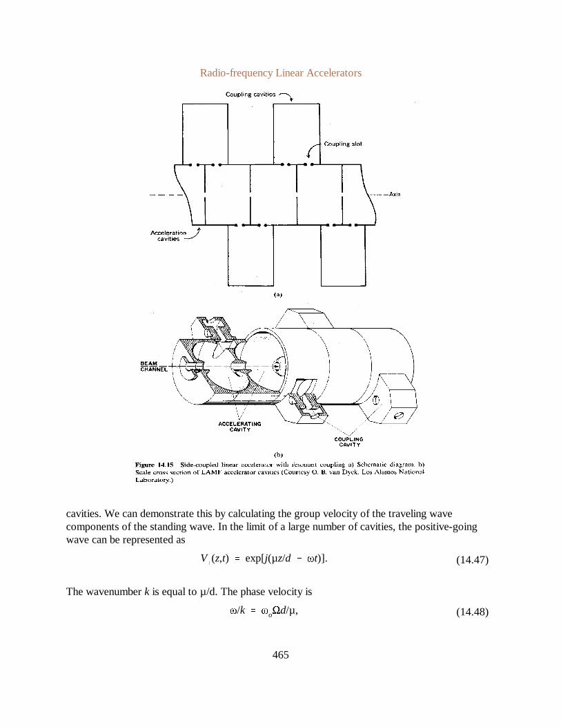
unexcited cavities to the side and pass the ion beam through the even-numbered cavities. The resultis aβλ/2 accelerator with good power coupling. The side-coupled linac [See B. C. Knapp, E. A.Knapp, G. J. Lucas, and J. M. Potter, IEEE Trans. Nucl. Sci.NS-12, 159 (1965)] isillustrated inFigure 14.15a. Intermediate cavities are coupled to an array of cylindrical cavities by magneticcoupling slots. Low-level electromagnetic oscillations in the side cavities act to transfer energyalong the system. There is little energy dissipation in the side cavities. Figure 14.15b illustrates animproved design. The side cavities are reentrant to make them more compact (see Section 12.2).The accelerator cavity geometry is modified from the simple cylinder to reduce shunt impedance.The simple cylindrical cavity has a relatively high shunt impedance because wall current at theoutside corners dissipates energy while making little contribution to the cavity inductance.
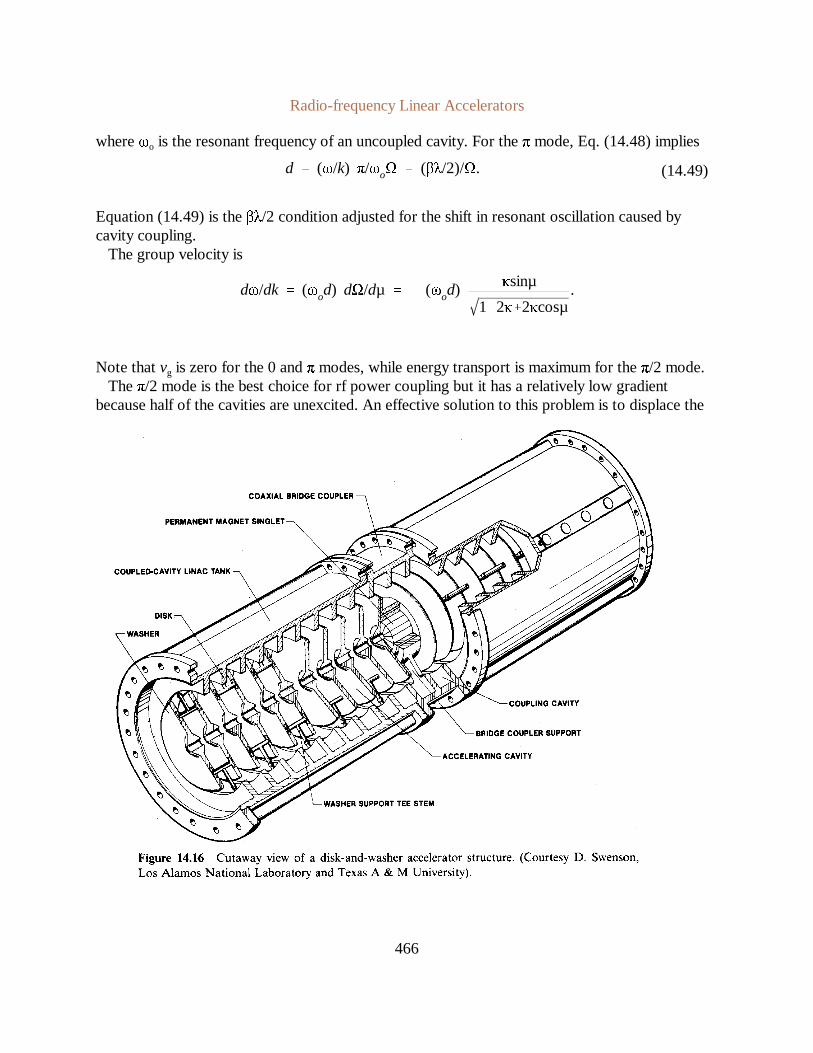
The disk and washer structure (Fig. 14.16) is an alternative to the side-coupled linac. It has highshunt impedance and good field distribution stability. Theaccelerating cavities are defined by"washers." The washers are suspended by supports connected to the wall along a radial electricfield null. The coupling cavities extend around the entire azimuth. The individual sections of thedisk-and-washer structure are strongly coupled. The perturbation analysis we used to treat coupled
Radio-frequency Linear Accelerators
470

Radio-frequency Linear Accelerators
471
Radio-frequency Linear Accelerators
472
Radio-frequency Linear Accelerators
473
d/vs π/ω. (14.51)
Ez(r,z,t) Eo cos(ωtφ). (14.52)
cavities is inadequate to determine the resonant frequencies of the disk-and-washer structure. Thedevelopment of strongly-coupled cavity geometries results largely from the application of digitalcomputers to determine normal modes.
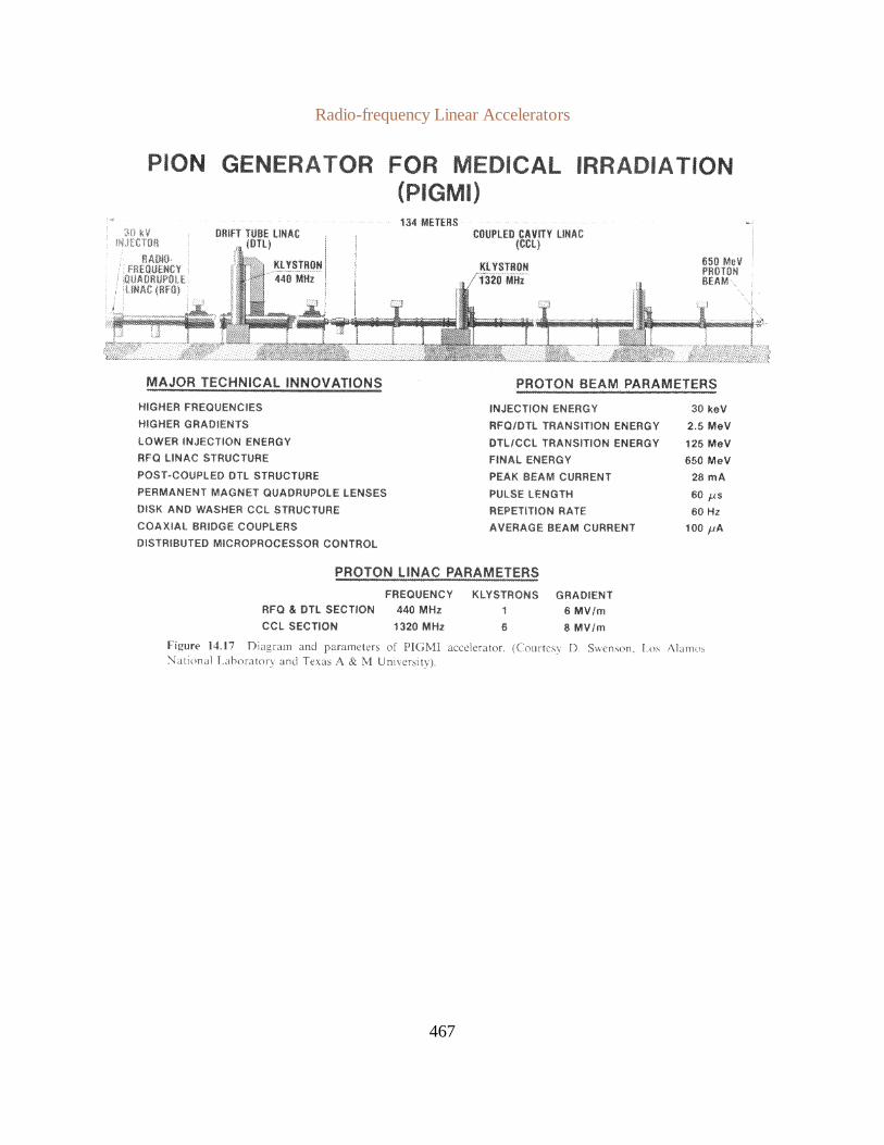
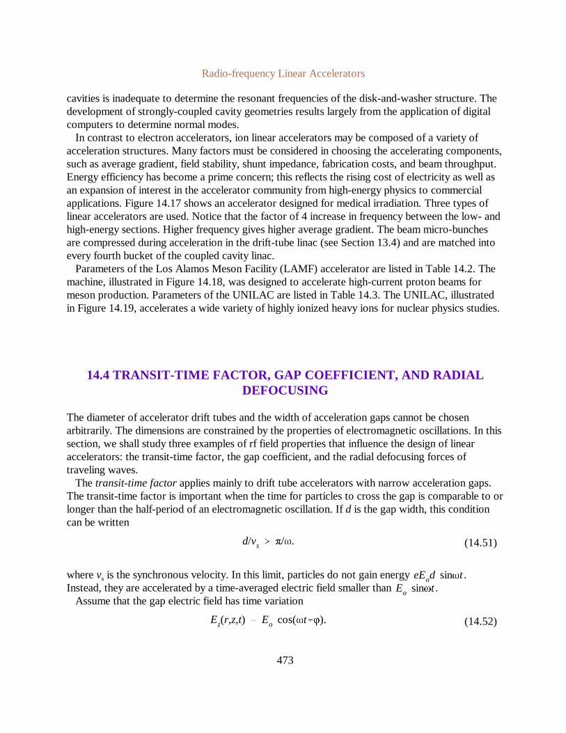
In contrast to electron accelerators, ion linear accelerators may be composed of a variety ofacceleration structures. Many factors must be considered in choosing the accelerating components,such as average gradient, field stability, shunt impedance, fabrication costs, and beam throughput.Energy efficiency has become a prime concern; this reflects the rising cost of electricity as well asan expansion of interest in the accelerator community from high-energy physics to commercialapplications. Figure 14.17 shows an accelerator designed for medical irradiation. Three types oflinear accelerators are used. Notice that the factor of 4 increase in frequency between the low- andhigh-energy sections. Higher frequency gives higher average gradient. The beam micro-bunchesare compressed during acceleration in the drift-tube linac (see Section 13.4) and are matched intoevery fourth bucket of the coupled cavity linac.
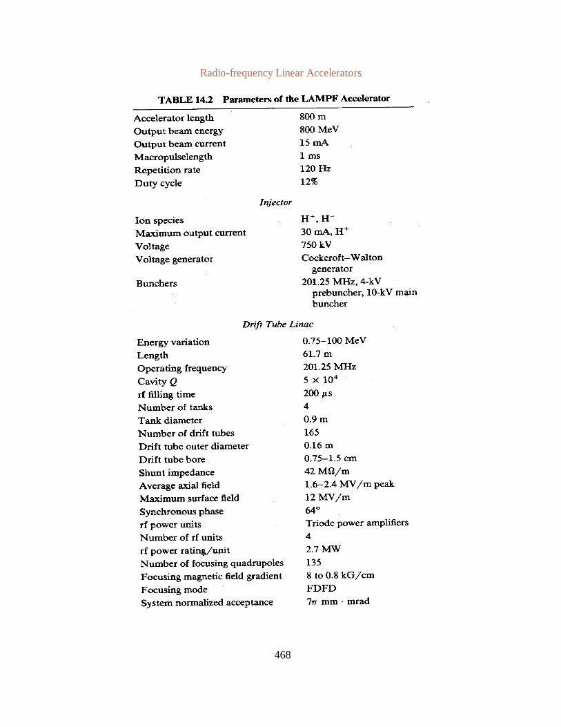
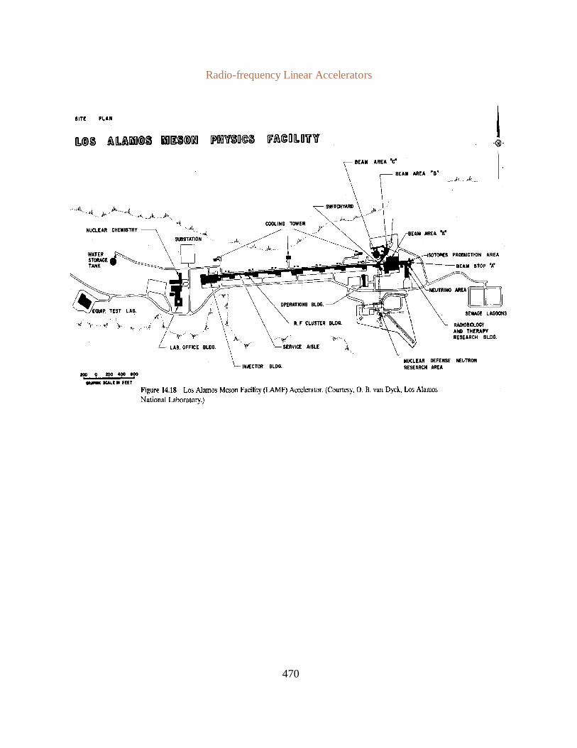
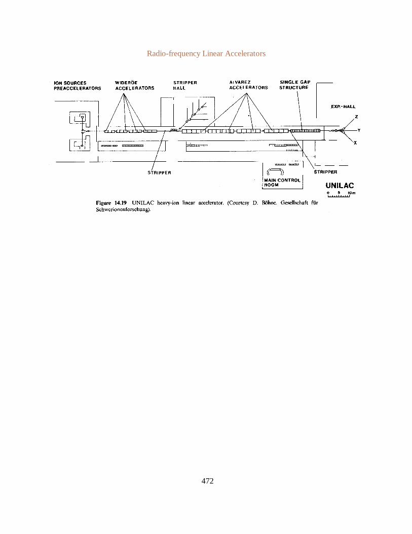
Parameters of the Los Alamos Meson Facility (LAMF)accelerator are listed in Table 14.2. Themachine, illustrated in Figure 14.18, was designed toaccelerate high-current proton beams formeson production. Parameters of the UNILAC are listed in Table 14.3. The UNILAC, illustratedin Figure 14.19, accelerates a wide variety of highly ionized heavy ions for nuclear physics studies.
14.4 TRANSIT-TIME FACTOR, GAP COEFFICIENT, AND RADIALDEFOCUSING
The diameter of accelerator drift tubes and the width of acceleration gaps cannot be chosenarbitrarily. The dimensions are constrained by the properties of electromagnetic oscillations. In thissection, we shall study three examples of rf field properties that influence the design of linearaccelerators: the transit-time factor, the gap coefficient, and the radial defocusing forces oftraveling waves.
The transit-time factorapplies mainly to drift tube accelerators with narrow acceleration gaps.The transit-time factor is important when the time for particles to cross the gap is comparable to orlonger than the half-period of an electromagnetic oscillation. Ifd is the gap width, this conditioncan be written
wherevs is the synchronous velocity. In this limit, particles do not gain energy .eEod sinωtInstead, they are accelerated by a time-averaged electric field smaller than .Eo sinωt
Assume that the gap electric field has time variation

Radio-frequency Linear Accelerators
474
dpz/dt qEo sin(ωtφ). (14.53)
∆pz qEo
d/2vs
d/2vs
cos(ωtφ)dt qEo
d/2vs
d/2vs
(cosωt sinφ sinωt cosφ)dt. (14.54)
∆pz (2qEo/ω) sin(d/2vs) sinφ. (14.55)
∆po qEo sinφ (d/vs). (14.56)
Tf ∆p/∆po sin(ωd/2vs)/(ωd/2vs). (14.57)
Tf sin(ω∆t/2)/(ω∆t/2). (14.58)
The longitudinal equation of motion for a particle crossing the gap is
Two assumptions simplify the solution of Eq. (14.53).
1.The timet = 0 corresponds to the time that the particle is at the middle of the gap.
2. The change in particle velocity over the gap is small compared tovs.
The quantityφ is equivalent to the particle phase in the limit of a gap of zero thickness (see Fig.13.1). The change in longitudinal motion is approximately
Note that the term involving sinωt is an odd function; its integral is zero. The total change inmomentum is
The momentum gain of a particle in the limit d 0 is
The ratio of the momentum gain for a particle in a gap with nonzero width to the ideal thin gap isdefined as the transit-time factor:
The transit-time factor is also approximately equal to the ratio of energy gain in a finite-width gapto that in a zero-width gap.
Defining a particle transit time as , Eq. (14.57) can be rewritten∆t d/vs
The transit-time factor is plotted in Figure 14.20 as a function of .ω∆tAs an application example, consider acceleration of 5 MeV Cs+ ions in a Wideröe accelerator
operating at f = 2 MHz. The synchronous velocity is 2.6 × 10⁶ m/s. The transit time across a 2-cmgap is∆t = 7.5 ns. The quantity equals 0.95; the transit-time factor is 0.963. If theω∆t

Radio-frequency Linear Accelerators
475
Ez(0,z,t) Eo sin(ωtωz/vs). (14.59)
Ez(0,z) Eo sin(2πz/λ), (14.60)
synchronous phase is 60 and the peak gap voltage is 100 kV, the cesium ions gain an averageenergy of (100)(0.963)(sin60) = 83 keV per gap.
Thegap coefficientcharacterizes the radial variation of accelerating fields across the dimensionof the beam. Variations in Ez lead to a spread in beam energy; particles with large-amplitudetransverse oscillations gain a different energy than particles on the axis. Large longitudinal velocityspread is undesirable for research applications and may jeopardize longitudinal confinement in rfbuckets. We shall first perform a non-relativistic derivation because the gap coefficient is primarilyof interest in linear ion accelerators.
The slow-wave component of electric field chiefly responsible for particle acceleration has theform
As discussed in Section 13.3, a slow wave appears to be an electrostatic field with no magneticfield when observed in a frame moving at velocityvs. The magnitude of the axial electric field isunchanged by the transformation. The on-axis electric field in the beam rest frame is

Radio-frequency Linear Accelerators
476
λ 2πvs/ω. (14.61)
Er(r,z) (r /2) (2π/λ) Eo cos(2πz/λ). (14.62)
Er(r,z) Eo [1 (πr /λ)2 sin(2πz/λ)] (14.63)
∆T/T (πrb/λ)2. (14.64)
λ > πrb/ ∆T/T. (14.65)
whereλ’ is the wavelength in the rest frame. In the nonrelativistic limit, so thatλ λ
The origin and sign convention in Eq. (14.60) are chosen so that a positive particle atz' = 0 haszero phase. In the limit that the beam diameter is small compared toλ’, the electrostatic field canbe described by the paraxial approximation. According to Eq. (6.5), the radial electric field is
The equation implies that × E 0
The energy gain of a particle at the outer radius of the beam (rb) is reduced by a factorproportional to the square of the gap coefficient:
The gap coefficient must be small compared to unity for a small energy spread. Equation (14.64)sets a limit on the minimum wavelength of electromagnetic waves in terms of the beam radius andallowed energy spread:
As an example, consider acceleration of a 10-MeV deuteron beam of radius 0.01m. To obtain anenergy spread less than 1%, the wavelength of the slow wave must be greater than 0.31 m. Using asynchronous velocity of 3 x 10⁷ m/s, the rf frequency must be lower than f < 100 MHz.
This derivation can also be applied to demonstrate radial defocusing of ion beams by the fields ofa slow wave. Equation (14.62) shows that slow waves must have radial electric fields. Note thatthe radial field is positive in the range of phase and negative in the range0 < φ < 90
. Therefore, the rf fields radially defocus particles in regions of axial stability.90 < φ < 180The radial forces must be compensated in ion accelerators by transverse focusing elements, usuallymagnetic quadrupole lenses. The stability properties of a slow wave are graphically illustrated inFigure 14.21. The figure shows three-dimensional variations of the electrostatic confinementpotential (see Section 13.3) of an accelerating wave viewed in the wave rest frame. It is clear thatthere is no position in which particles have stability in both the radial and axial directions.

Radio-frequency Linear Accelerators
477
λ λ/γ, (14.66)
E
r (r ,z) E
o (r /2) (2π/γλ) cos(2πz/γλ), (14.67)
E
z(r ,z) E
o [1 (πr /γλ)2] sin(2πz/γλ). (14.68)
The problems of the gap coefficient and radial defocusing are reduced greatly for relativisticparticles. For a relativistic derivation, we must include the fact that the measured wavelength of theslow wave is not the same in the stationary frame and the beam rest frame. Equation (2.23) impliesthat the measurements are related by
whereγ is the relativistic factor, . Again, primed symbols denote theγ 1/ 1 (vs/c)2
synchronous particle rest frame.The radial and axial fields in the wave rest frame can be expressed in terms of the stationary
frame wavelength:
Note that the peak value of axial field is unchanged in a relativistic transformation ( ).E
o EoTransforming Eq. (14.68) to the stationary frame, we find that

Radio-frequency Linear Accelerators
478
Ez(r,z) Eo [1 (πr/γλ)2] sin(2πz/λ), (14.69)
E
r γ (Er vzBθ). (14.70)
Fr q (Er vzBθ). (14.71)
Fr [Eo (r/2) (2π/λ) cos(2πz/λ)]/γ2. (14.72)
with the replacement . Equation (14.69) differs from Eq. 14.63 by theγ factor inr r , z z/γthe denominator of the gap coefficient. The radial variation of the axial accelerating field isconsiderably reduced at relativistic energies.
The transformation of radial electric fields to the accelerator frame is more complicated. A pureradial electric field in the rest frame corresponds to both a radial electric field and a toroidalmagnetic field in the stationary frame:
Furthermore, the total radial force exerted by the rf fields on a particle is written in the stationaryframe as
The net radial defocusing force in the stationary frame is
Comparison with Eq. (14.62) shows that the defocusing force is reduced by a factor ofγ2. Radialdefocusing by rf fields is negligible in high-energy electron linear accelerators.
14.5 VACUUM BREAKDOWN IN RF ACCELERATORS
Strong electric fields greater than 10 MV/m can be sustained in rf accelerators. This results partlyfrom the fact that there are no exposed insulators in regions of high electric field. In addition, rfaccelerators are run at high duty cycle, and it is possible to condition electrodes to remove surfacewhiskers. The accelerators are operated for long periods of time at high vacuum, minimizingproblems of surface contamination on electrodes.
Nonetheless, there are limits to the voltage gradient set by resonant particle motion in theoscillating fields. The process is illustrated for electrons in anacceleration gap in Figure 14.22. Anelectron emitted from a surface during the accelerating half-cycle of the rf field can be acceleratedto an opposing electrode. The electron produces secondary electrons at the surface. If thetransit time of the initial electron is about one-half that of the rf period, the electric field will be in a

Radio-frequency Linear Accelerators
479
direction to accelerate the secondary electrons back to the first surface. If the secondary electroncoefficientδ is greater than unity, the electron current grows. Table 14.4 shows maximumsecondary electron coefficients for a variety of electrode materials. Also included are the incidentelectron energy corresponding to peak emission and toδ = 1. Emission falls off at a higher electronenergy. Table 14.4 gives values for clean, outgassed surfaces. Surfaces without special cleaningmay have a value ofδ as high as 4.
The resonant growth of electron current is called multipactoring, implying multiple electronimpacts. Multipactoring can lead to a number of undesirable effects. The growing electron currentabsorbs rf energy and may clamp the magnitude of electric fields at the multipactoring level.Considerable energy can be deposited in localized regions of the electrodes, resulting in outgassingor evaporation of material. This often leads to a general cavity breakdown.
Radio-frequency Linear Accelerators
480
E(x,t) Eo sin(ωtφ). (14.73)
me (d 2x/dt 2) eEo sin(ωtφ). (14.74)
x (eEo/meω2) [ωtcosφ sinφ sin(ωtφ)]. (14.75)
∆t (2n1) (π/ω). (14.76)
d (eEo/meω2) [(2n1) π cosφ 2sinφ], (14.77)
vx(xd) (2eEo/meω2) cosφ. (14.78)
0 < φ < π/2. (14.79)
Conditions for electron multipactoring can be derived easily for the case of a planar gap withelectrode spacingd. The electric field inside the gap is assumed spatially uniform with timevariation given by
The non-relativistic equation of motion for electrons is
The quantityφ represents the phase of the rf field at the time an electron is produced on anelectrode. Equation (14.74) can be integrated directly. Applying the boundary conditions thatx = 0and dx/dt = 0 at t = 0, we find that
Resonant acceleration occurs when electrons move a distanced in a time interval equal to an oddnumber of rf half-periods. When this condition holds, electrons emerging from the impactedelectrode are accelerated in the -x direction; they follow the same equation of motion as the initialelectrons. The resonance condition is
for n = 0, 1, 2, 3,.... Combining Eqs. (14.75) and (14.76), the resonant condition can be rewritten
because . Furthermore, we can use Eq. (14.75) to find the velocity ofsin(ω∆tφ) sinφelectrons arriving at an electrode:
The solution of Eq. (14.74) is physically realizable only for particles leaving the initial electrodewithin a certain range ofφ. First, the electric field must be negative to extract electrons from thesurface att = 0, or sinφ > 0. A real solution exists only if electrons arrive at the opposite electrodewith positive velocity, or cosφ > 0. These two conditions are met in the phase range

Radio-frequency Linear Accelerators
481
Vo (dω)2me/πe (2πd/λ)2 (mec2)/πe. (14.80)
Figure 14.23 is a plot of Eq. (14.77) showing the breakdown parameter versus the rf(eEo/meω2d)
phase at which electrons leave the surface. Electron resonance is possible, in principle, over arange of gap voltage from 0 to .V meω
2d 2/2eElectron multipactoring is a significant problem in the low-energy sections of linear ion
accelerators. Consider, for example, an acceleration gap for 2-MeV protons. Assume that theproton transit time∆t is such that . This implies that . Substituting the aboveω∆t 1 ωd βccondition in Eq. (14.78) and taking then = 0 resonance condition, the electron energy at impact is
The quantityβ equals 0.065 for 2-MeV protons. The peak electronEc (2/π2) (βcosφ)2 (mec2).
energy occurs when cosφ = 1 (φ = 0); for the example it is 440 eV. Table 14.4 shows that thisvalue is close to the energy of peak secondary electron emission. Electrons emitted at other phasesarrive at the opposing electron with lower energy; therefore, they are not as likely to initiate aresonant breakdown. For this reason, the electron multipactoring condition is often quoted as
Equation (14.80) is expressed in terms ofλ, the vacuum wavelength of the rf oscillations.Electron multipactoring for the case quoted is probably not significant for values ofn greater
than zero because the peak electron energy is reduced by a factor of about 2n2. Therefore,breakdowns are usually not observed until the gap reaches a voltage level near that of Eq. (14.80).For an rf frequency f = 400 MHz, an acceleration gap 0.8 cm in width hasω∆t = 1 for 2-MeV
Radio-frequency Linear Accelerators
482
VK (2πd/λ)2 (mpc2)/πe. (14.81)
protons. This corresponds to a peak voltage of 730 V. At higher field levels, the resonancecondition can be met over longer pathlengths at higher field stresses. This corresponds tohigh-energy electrons, which generally have secondary emission coefficients less than unity.Therefore, with clean surfaces it is possible to proceed beyond multipactoring by raising the rfelectric field level rapidly. This may not be the case with contaminated electrodes; surface effectscontribute much of the mystery and aggravation associated with rf breakdown.
The ultimate limits for rf breakdown in cleanacceleration gaps were investigated experimentallyby Kilpatrick [W.D. Kilpatrick, "Criterion for Vacuum Sparking to Include Both RF and DC,"University of California Radiation Laboratory, UCRL-2321, 1953]. The following formula isconsistent with a wide variety of observations:
Note that Eq. (14.81) is identical to Eq. 14.80 with the replacement of the electron mass by that ofthe proton. The Kilpatrick voltage limit is about a factor of2000 times the electron multipactoringcondition. The similarity of the equations suggests proton multipactoring as a mechanism forhigh-voltage rf breakdown. The precise mechanisms of proton production on electrode surfacesare unknown. Proton production may be associated with thin surface coatings. Present research onextending rf systems past the Kilpatrick limit centers on the use of proton-free electrodes.
14.6 RADIO-FREQUENCY QUADRUPOLE
The rf quadrupole [I.M. Kapchinskii and V. A. Teplyakov, Priboty i Teknika Eksperimenta2, 19(1970); R. H. Stokes, K. R. Crandall, J. E. Stovall, and D. A. Swenson, IEEE Trans. Nucl. Sci.NS-26, 3469 (1979)] is an ion accelerator in which both acceleration and transverse focusing areperformed by rf fields. The derivations of Section 14.4 (showing lack of absolute stability in an rfaccelerator) were specific to a cylindrical system; the fields in an RFQ are azimuthally asymmetric.There is no moving frame of reference in which RFQ fields can be represented as an electrostaticdistribution. We shall see that the electric fields in the RFQ consist of positive and negativetraveling waves; the positive wave continually accelerates ions in the range of stable phase. Thebeam is focused by oscillating transverse electric field components. These fields provide net beamfocusing if the accelerating fields are not too high.
The major application of the RFQ is in low-energy ion acceleration. In the past, low-velocity ionacceleration presented one of the main technological difficulties for high-flux accelerators. Aconventional ion beam injector consists of an ion source floating at high voltage and anelectrostatic acceleration column. Space charge forces are strong for low-velocity ion beams; this

Radio-frequency Linear Accelerators
483
Ex(x,y,z,t) (Eox/a) sinωt, (14.82)
Ey(x,y,z,t) (Eoy/a) sinωt. (14.83)
fact motivates the choice of a high injection voltage, typically greater than 1 MV. The resultingsystem with adequate insulation occupies a large volume. The extracted beam must be bunched forinjection into an rf accelerator. This implies long transport sections with magnetic quadrupolelenses. Magnetic lenses are ineffective for focusing low-energy ion beams, so that flux limits arelow.
In contrast, the RFQ relies on strong electrostatic focusing in a narrow channel; this allowsproton beam current in the range of 10 to 100 mA. An additional advantage of the RFQ is that itcan combine the functions of acceleration and bunching. This is accomplished by varying thegeometry of electrodes so that the relative magnitudes of transverse and longitudinal electric fieldsvary through the machine. A steady-state beam can be injected directly into the RFQ and reversiblybunched while it is being accelerated.
The quadrupole focusing channel treated in Chapter 8 has static fields with periodicallyalternating field polarity along the beam axis. In order to understand the RFQ, we will consider thegeometry illustrated in Figure 14.24. The quadrupole electrodes are axially uniform but havetime-varying voltage of the form . It is valid to treat the fields near the axis in theVosinωtelectrostatic limit if , wherea is the distance between the electrodes and the axis. In thisa « c/ωcase, the electric fields are simply the expressions of Eqs. (4.22) and (4.23)multiplied by sinωt:
The oscillating electric fields near the axis are supported by excitation of surrounding microwavestructures. Off-axis fields must be described by the full set of Maxwell equations.

Radio-frequency Linear Accelerators
484
m (d 2x/dt 2) (qEox/a) sinωt. (14.84)
x(t) x0 sinΩt x1 sinωt. (14.85)
x1 « x0, (14.86)
Ω « ω, (14.87)
Ω2x0 « ω2x1. (14.88)
Ω2x0 sinΩt ω2x1 sinωt (qEo/ma) sinωt (x0 sinΩt x1 sinωt). (14.89)
ω2x1 [qEox0sin(Ωt)/a]/m
x1 [qEox0sin(Ωt)/a]/mω2. (14.90)
The non-relativistic equation for particle motion in the x direction is
Equation (14.84) can be solved by the theory of the Mathieu equations. We will take a simplerapproach to arrive at an approximate solution. Assume that the period for a transverse particleorbit oscillation is long compared to . In this limit, particle motion has two components; a2π/ωslow betatron oscillation (parametrized by frequencyΩ) and a rapid small-amplitude motion atfrequencyω. We shall seek a solution by iteration using the trial solution
where
Substituting Eq. (14.85) into Eq. (14.84), we find that
The first term on the left-hand side and the second term on the right-hand side of Eq. (14.89) aredropped according to Eqs. (14.88) and (14.86). The result is an equation for the high-frequencymotion:
or
The second step is to substitute Eq. (14.90) into Eq. (14.84) and average over a fast oscillationperiod to find the long-term motion. Terms containing sinωt average to zero. The remaining termsimply the following approximate equation forx0:

Radio-frequency Linear Accelerators
485
Ω2x0 sinΩt (qEo/ma)2 (x0sinΩt) (sin2ωt)/ω2, (14.91)
Ω (eEo/maω)/ 2. (14.92)
where denotes the average over a time 2π/ω. Equation (14.91) implies thatΩ has the realsin2ωtvalue
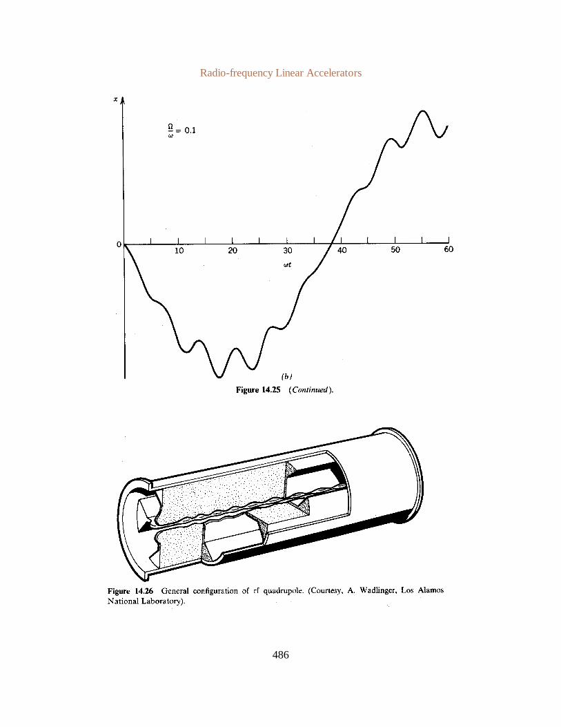
The long-term motion is oscillatory; the time-varying quadrupole fields provide net focusing.Numerical solutions to Eq. (14.84) are plotted in Figure 14.25 for and . The phaseω3Ω ω10Ωrelationship of Eq. (14.90) guarantees that particles are at a larger displacement when the fields arefocusing. This is the origin of the average focusing effect. Orbit solutions in the y direction aresimilar.
Radio-frequency Linear Accelerators
486
Radio-frequency Linear Accelerators
487
Ex(x,y,z,t) (Eox/a) [1 ε sin(2πz/D)] sinωt, (14.93)
Ey(x,y,z,t) (Eoy/a) [1 ε sin(2πz/D)] sinωt. (14.94)
Ez/z (Ex/x Ey/y). (14.95)
Ez(x,y,z,t) (2εEoD/2πa) cos(2πz/D) sinωt. (14.96)
Ez (εEoD/2πa) [sin(2πz/Dωt) sin(2πz/Dωt)]. (14.97)
vs Dω/2π. (14.98)
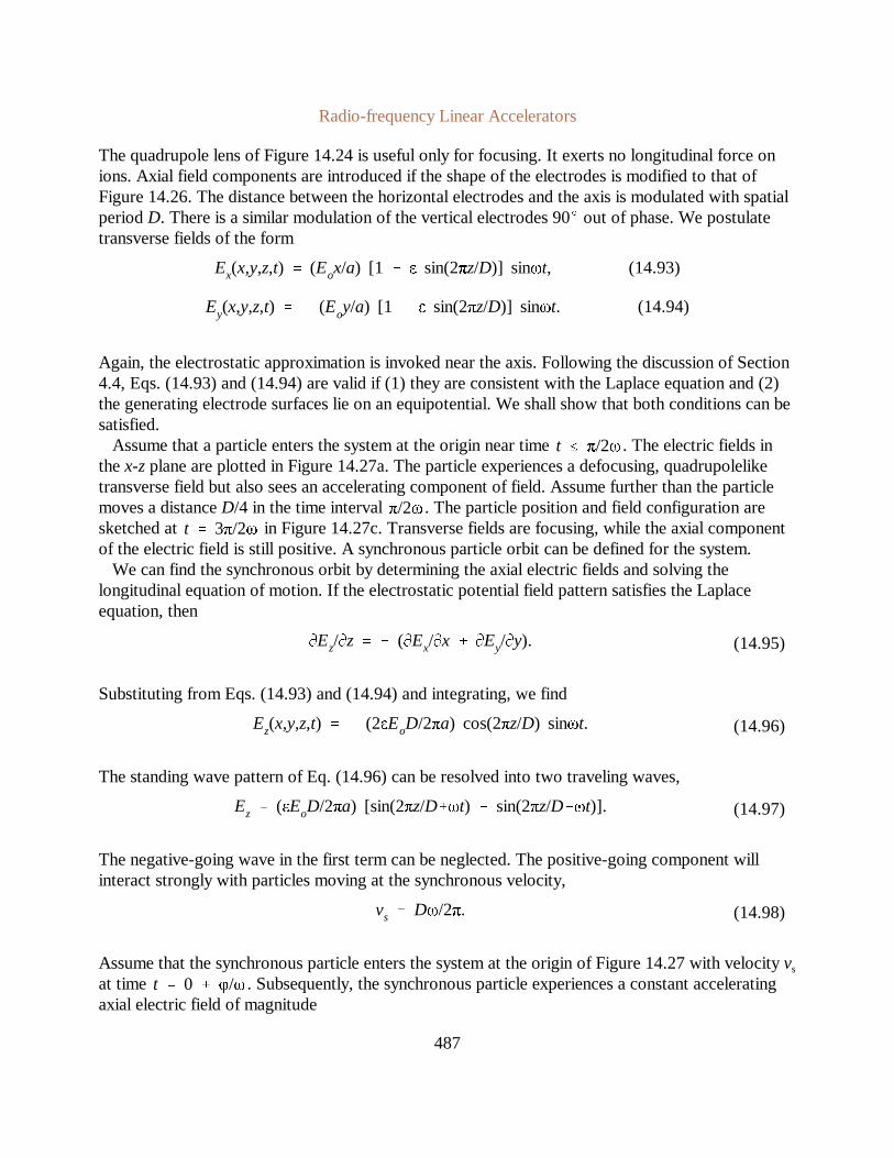
The quadrupole lens of Figure 14.24 is useful only for focusing. It exerts no longitudinal force onions. Axial field components are introduced if the shape of the electrodes is modified to that ofFigure 14.26. The distance between the horizontal electrodes and the axis is modulated with spatialperiodD. There is a similar modulation of the vertical electrodes 90 out of phase. We postulatetransverse fields of the form
Again, the electrostatic approximation is invoked near the axis. Following the discussion of Section4.4, Eqs. (14.93) and (14.94) are valid if (1) they are consistent with the Laplace equation and (2)the generating electrode surfaces lie on an equipotential. We shall show that both conditions can besatisfied.
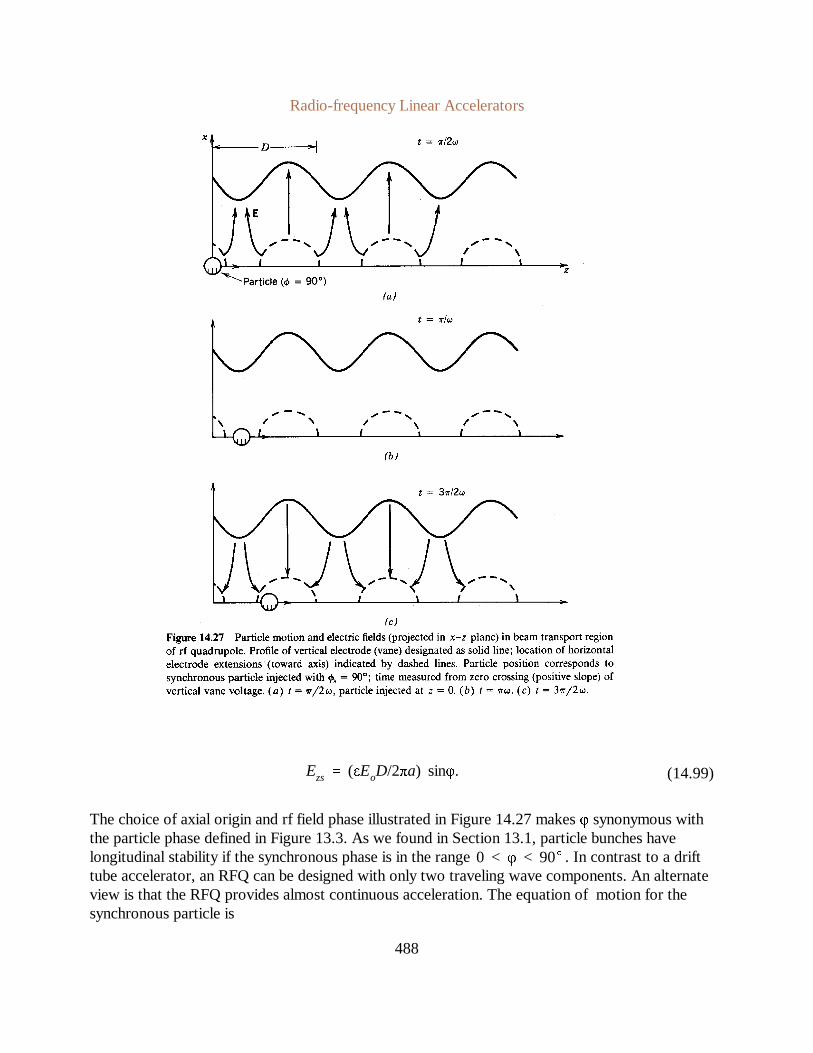
Assume that a particle enters the system at the origin near time . The electric fields int π/2ωthex-zplane are plotted in Figure 14.27a. The particle experiences a defocusing, quadrupoleliketransverse field but also sees an accelerating component of field. Assume further than the particlemoves a distanceD/4 in the time interval . The particle position and field configuration areπ/2ωsketched at in Figure 14.27c. Transverse fields are focusing, while the axial componentt 3π/2ωof the electric field is still positive. A synchronous particle orbit can be defined for the system.
We can find the synchronous orbit by determining the axial electric fields and solving thelongitudinal equation of motion. If the electrostatic potential field pattern satisfies the Laplaceequation, then
Substituting from Eqs. (14.93) and (14.94) and integrating, we find
The standing wave pattern of Eq. (14.96) can be resolved into two traveling waves,
The negative-going wave in the first term can be neglected. The positive-going component willinteract strongly with particles moving at the synchronous velocity,
Assume that the synchronous particle enters the system at the origin of Figure 14.27 with velocityvs
at time . Subsequently, the synchronous particle experiences a constant acceleratingt 0 φ/ωaxial electric field of magnitude
Radio-frequency Linear Accelerators
488
Ezs (εEoD/2πa) sinφ. (14.99)
The choice of axial origin and rf field phase illustrated in Figure 14.27 makesφ synonymous withthe particle phase defined in Figure 13.3. As we found in Section 13.1, particle bunches havelongitudinal stability if the synchronous phase is in the range . In contrast to a drift0 < φ < 90tube accelerator, an RFQ can be designed with only two traveling wave components. An alternateview is that the RFQ provides almost continuous acceleration. The equation of motion for thesynchronous particle is

Radio-frequency Linear Accelerators
489
m (dvs/dt) (εqEoD/2πa) sinφ. (14.100)
dD/dz (2πεqEosinφ/mω2a). (14.101)
d 2x/dt 2 (qEox/ma) [1 ε sin(2πz/D)] sin(ωtφ)
(qEox/ma) sin(ωtφ) (εqEox/2ma) [cos(2πz/Dωtφ) cos(2πz/Dωtφ)].(14.102)
d 2x/dt 2 (qEox/ma) sin(ωtφ) (εqEox/2ma) cosφ. (14.103)
x(t) x0 cosΩt
Ω ½(qEo/maω)2 (εqEo/2ma) cosφ
Substituting from Eq. (14.98), Eq. (14.100) can be rewritten as
If the field modulation factorε is constant, Eq. (14.101) indicates that the length of modulationsshould increase linearly moving from entrance to exit of the RFQ.
The transverse equation of motion for a particle passingz = 0 at timeφ/ω is
Again, we retain only the part of the force resonant with synchronous particles. Applying thesynchronous condition [Eq. (14.98)], Eq. (14.102) becomes
The first term on the right-hand side represents the usual transverse focusing from the rfquadrupole. This component of motion is solved by the same method as the axially uniformoscillating quadrupole. The second term represents a defocusing force arising from the axialmodulation of the quadrupole electrodes. The origin of this force can be understood by inspectionof Figure 14.27. A sequence of particle position and electrode polarities is shown for a particle witha phase near 90. On the average, the electrode spacing in thex direction is smaller duringtransverse defocusing and larger during the focusing phase for . This brings about aφ < 90reduction of the average focusing force.
The solution for average betatron oscillations of particles is
where
Radio-frequency Linear Accelerators
490
ε qEo/(maω2 cosφ). (14.105)
Ez (qE2oD tanφ)/(2πa 2mω2). (14.106)
Φ(x,y,z) (Eox2/2a) [1 ε sin(2πz/D)]
(Eoy2/2a) [1 ε sin(2πz/D)] (εEoD
2/4π2a) sin(2πz/D).(14.107)
x2min [a 2
(εD 2/2π2) sin(2πz/D)]/[1 ε sin(2πz/D)].
The same result is determined for motion in they direction. There is net transverse focusing ifΩ is areal number, or
The longitudinal electric field is proportional toε. Therefore, there are limits on theacceleratinggradient that can be achieved while preserving transverse focusing:
Note that high longitudinal gradient is favored by high pole tip field (Eo) and a narrow beam channel(a).
The following parameters illustrate the results for the output portion of a 2.5-MeV RFQoperating at 440 MHz. The channel radius is a = 0.0025 m, the synchronous phase is , theφ 60cell length is 0.05 m, and the pole tip field is 10 MV/m, well below the Kilpatrick limit. The limitinglongitudinal gradient is 4.4 MV/m. The corresponding modulation factor isε = 0.05. A typical RFQdesign accelerates protons to 2.5 MeV in a length less than 2 m.
Equations (14.93), (14.94), and (14.96) can be used to find the electrostatic potential functionfollowing the same method used in Section 4.4. The result is
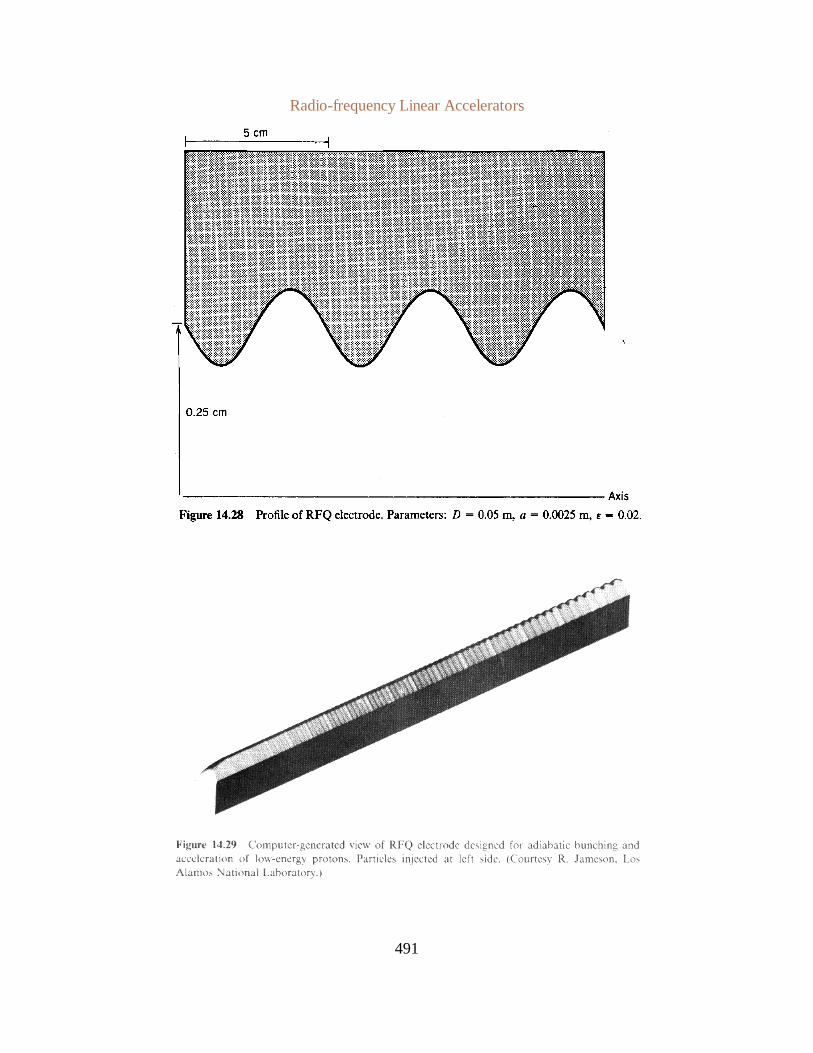
The equipotential surfaces determine the three-dimensional electrode shape. TheΦ ±Eoa/2equation for the minimum displacement of the vertical vanes from the axis is
This function is plotted in Figure 14.28. For a modulation factorε = 0.02 and an average minimumelectrode displacement of 0.0025 m, the distance from the electrode to the axis varies between0.0019 and 0.0030 m.
The design of RFQ electrodes becomes more complex if the modulation factor is varied to addbunching capability. The design procedure couples results from particle orbit computer codes into acomputer-controlled mill to generate complex electrodes such as that illustrated in Figure 14.29.The structure transports an incoming 30-mA, 30-keV proton beam. Electrode modulations increasegradually along the direction of propagation, adding longitudinal field components. Thesynchronous phase rises from 0 to the final value. Note the increasing modulation depth and cell
Radio-frequency Linear Accelerators
491

Radio-frequency Linear Accelerators
492

Radio-frequency Linear Accelerators
493
length along the direction of acceleration.A cross section of a complete RFQ is illustrated in Figure 14.30. The volume outside the
transport region is composed of four coupled cylindrical section cavities. The desired excitationmodes for the cavities have axial magnetic fields and properties which are uniform along thelongitudinal direction. Field polarities and current flows are illustrated for the quadrupole mode. A440-MHz cavity has a radius of about 0.2 m. The mode for the quadrupole oscillation in all fourcavities is designated TE210. This terminology implies the following:
1. Electric fields are transverse to the z direction in the rf portion of the cavity.
2. Field quantities vary in azimuth according to cos(2θ).
3. The electric field is maximum on axis and decreases monotonically toward the wall.
4. There is no axial variation of field magnitudes in the standing wave.
Coupling of the four lines through the narrow transport region is not strong; equal distribution ofenergy demands separate drives for each of the lines. The usual procedure is to surround the RFQwith an annular resonator (manifold) driven at a single feed point. The manifold symmetrizes the rfenergy; it is connected to the transmission lines by multiple coupling slots.
Other modes of oscillation are possible in an RFQ cavity. The dipole mode illustrated in Figure14.30b is particularly undesirable since it results in electrostatic deflections and beam loss. Thedipole mode frequency does not differ greatly from that of the quadrupole. Another practicalproblem is setting end conditions on the electrodes to maintain a uniform electric field magnitudeover the length. Problems of mode coupling and field uniformity multiply as the length of the RFQincreases. This is the main reason why RFQ applications are presently limited to low-energyacceleration. The RFQ has been studied as a pre-accelerator for heavy ions. In this case, thefrequency is low. Low-frequency RFQs are sometimes fabricated as a nonresonant structuredriven by an oscillator like the Wideröeaccelerator.
14.7 RACETRACK MICROTRON
The extensive applications of synchrotron radiation to atomic and solid-state physics research hasrenewed interest in electron accelerators in the GeV range. The microtron is one of the mostpromising electron accelerators for research. Its outstanding feature is the ability to generate acontinuous beam of high-energy electrons with average current approaching 100 µA. The time-average output of a microtron is much higher than a synchrotron or high-electron linac, whichproduce pulses of electrons at relatively low repetition rates.
The racetrack microtron [V.Veksler, Compt. Rend. Acad. Sci. U. S. S. R.43, 444 (1944)] isillustrated in Figure 14.31a. Electrons areaccelerated in a short linac section. Uniform field sector
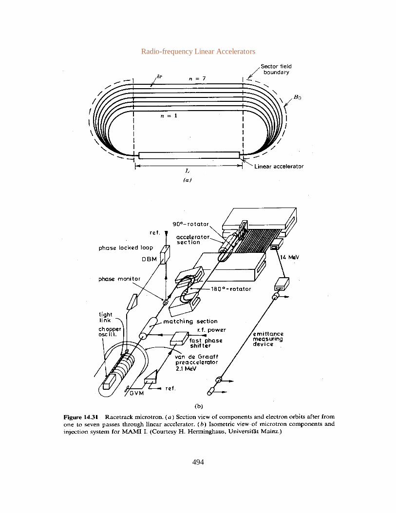
Radio-frequency Linear Accelerators
494
Radio-frequency Linear Accelerators
495
Ez Eo sin(ωt ωz/c).
∆U eEoL sinφ,
∆tn 2L/c 2πrgn/c, (14.108)
magnets at each end of the accelerator confine the electrons. Electrons at a variety of energy levelsare contained simultaneously in the machine. Electron orbits in the magnets are half-circles. It iseasily demonstrated that electrons return to the linear accelerator axis after each revolution,independent of their energy. The size of the orbit increases as the electron energy increases.
The microtron combines linear accelerator technology with circular accelerator particle dynamics.Beam recirculation allows more efficient utilization of the linac. In contrast to the high-energyelectron linear accelerators of Section 14.1 (where the machine length is a major constraint),acceleration gradient is not the primary concern in the microtron. This means that the acceleratorneed not operate at high field stress; therefore, power dissipation is a factor of 25-100 times lowerthan a high-gradient electron linac. This accounts for the capability of CW steady-state operation.The phase velocity of traveling wave components in the microtron linac is equal to the speed oflight. In contrast to high-energy electron linacs, microtrons have phase stability. The orbit size (and,hence, the time to return to the linac) depends on electron energy. Therefore, electrons can belongitudinally confined during acceleration, even at low values of accelerating gradient.
Some parameters of a medium-energy microtron are listed in Table 14.5. The machine is designedas a pre-accelerator in a three-microtron facility to produce an840-MeV beam. The 14-MeVniicrotron with its associated injection and extraction system is illustrated in Figure 14.31b. Theinjected beam is generated by a 2-MV Van de Graaff accelerator. A beam chopper in the terminal ofthe electrostatic accelerator produces short pulses of electrons phased-matched to the linac. Thecomplex series of lenses and deflection magnets matches the transverse and longitudinaldistributions of the electron beam to the acceptance of the microtron. The origin of the parametersin Table 14.5 will be evident after we develop the theory of microtron equilibrium orbits.
In order to describe the microtron analytically, assume that the sector fields have sharp boundariesand a uniform field magnitude,Bo. Electrons are injected with initial total energyUo and gain anenergy∆U in each pass through the linear accelerator. Assume, further, that , so that theUo » mec
2
electron velocity is always approximately equal to the speed of light. We have shown thatacceleration in linear accelerators arises from a traveling wave component of the form
The energy gain of a relativistic electron traversing an accelerator of lengthL is
whereφ is the phase of the particle with respect to the traveling wave. The energy gain forsynchronous electrons passing through the linac is independent of their total energy.
The indexn designates the number of times that an electron has passed through the linearaccelerator; the orbits in Figure 14.31 are labeled accordingly. The time for an electron to traversethe microtron is

Radio-frequency Linear Accelerators
496
rgn γnmec/eBo Un/eBoc.
Un Uo n∆U. (14.109)
∆tn 2L/c 2πUn/eBoc2 m(2π/ω). (14.110)
where
The quantity U is the total energy of an electron on thenth orbit:
The condition for synchronous electrons is that they arrive at the entrance to the linac at the samephase of the rf period. In other words, the traversal time must be an integer multiple of the rfperiod. Lettingω be the frequency of rf oscillations in the linac, this condition is written
Radio-frequency Linear Accelerators
497
∆tn ∆tn1 2π∆U/eBoc2. (14.111)
2π∆U/eBoc2 q (2π/ω). (14.112)
δr 2∆rg ∆U/eBoc.
As electrons gain energy, the particle velocity is constant but the orbit size increases. The traversaltime of high-energy particles is longer than that of low-energy particles. The difference in traversaltimes between particles on then andn-1 orbits is
Clearly, for synchronization∆tn must also equal an integer multiple of the rf period:
As an example, we pickq = 1. This means that electrons take one extra rf period for a traversal witheach energy increment. Following Table 14.5, assume a 20-turn microtron with an injection energyof 2 MeV. The bending magnetic field is 0.1 T, and the linear accelerator length is 0.8 M. Theenergy gain per turn is∆U = 0.6 MeV, implying an average acceleration gradient of 0.75 MV/m.Substituting into Eq. (14.112), the matched frequency isω = 1.5 × x 1010 s-1, or f = 2.4 GHz.Electrons injected at 2 MeV are boosted to 2.6 MeV in their first passage through the linac. Theinitial gyroradius in the bending field is 0.174 m; the total distance around the system on the firstorbit is 2.7 m. Equation 14.111 implies that the time for the first traversal equals 22 rf periods. Thisis a high number; the particle must return to the linac entrance with equal phase after an interval of
. Synchronization requires excellent bending field uniformity and a constant energy input22(2π/ω)beam with little velocity dispersion. The problem becomes more acute as electrons are accelerated.Electrons on the highest-energy orbit take 42 rf periods to traverse the system. The synchronizationproblem limits the practical number of turns in a single niicrotron. A choice ofq > 1 worsens theproblem.
The separation between adjacent orbits on the side opposite the linac is
For the parameters of the example,δr = 0.04 in. The large orbit separation makes extraction ofhigh-energy electrons relatively easy.
The two main problems of rnicrotrons are beam steering and beam breakup instabilities.Regarding the first problem, the uniform magnetic field of the microtron has horizontal focusing butno vertical focusing. Lenses must be added to each beam line on the straight sections opposite theaccelerator. Even with the best efforts to achieve bending field uniformity, it is necessary to addbeam steering magnets with active beam sensing and compensation to meet the synchronizationcondition. The beam breakup instability is severe in the microtron because the current of all beamsis concentrated in the high-Q resonant cavities of the linear accelerator. The beam breakupinstability is the main reason why microtron average currents are limited to less than 1 mA. Ithas also impeded the development of microtrons with superconducting linear accelerator cavities.These cavities have extremely high values of Q for all modes.

Radio-frequency Linear Accelerators
498
Phase stability is an interesting feature of microtrons. In contrast to high-energy electron linearaccelerators, variations of electron energy lead to phase shifts because of the change in orbitpathlength. For instance, a particle with energy greater than that of the synchronous particle has alarger gyroradius; therefore, it enters the linac with increased phase. For longitudinal stability, thehigher-energy electrons must receive a reduced energy increment in the linac. This is true if thesynchronous phase is in a region of decreasing field, . Particle phase orbits are90 φs 180the inverse of those in a linear ion accelerator.
Radio-frequency Linear Accelerators
499
The double-sided microtron (DSM) illustrated in Figure 14.32a is an alternative to the racetrackniicrotron. The DSM has linear accelerators in both straight sections. Beam deflection is performedby four 45 sector magnets. The major advantage, compared to the racetrack microtron, is thatapproximately double the electron energy can be achieved for the same magnet mass. The 45
sector magnet has the feature that the orbits of electrons of any energy are reflected at exactly 90
(see Fig. 14.32b).Unfortunately, the DSM has unfavorable properties for electron focusing. Figure 14.32c shows a
particle trajectory on the main orbit compared to an orbit displaced horizontally off-axis. Note thatthere is no focusing; the DSM has neutral stability in the horizontal direction. Furthermore, thesector magnets contribute defocusing forces in the vertical direction. There are edge-focusingeffects because the magnets boundaries are inclined 45 to the particle orbits. Reference to Section6.9, shows that the inclination gives a negative focal length resulting in defocusing.

Cyclotrons and Synchrotrons
500
15
Cyclotrons and Synchrotrons
The termcircular acceleratorrefers to any machine in which beams describe a closed orbit. Allcircular accelerators have a vertical magnetic field to bend particle trajectories and one or moregaps coupled to inductively isolated cavities to accelerate particles. Beam orbits are often not truecircles; for instance, large synchrotrons are composed of alternating straight and circular sections.The main characteristic of resonant circular accelerators is synchronization between oscillatingacceleration fields and the revolution frequency of particles.
Particle recirculation is a major advantage of resonant circular accelerators over rf linacs. In acircular machine, particles pass through the same acceleration gap many times (102 to greater than108). High kinetic energy can be achieved with relatively low gap voltage. One criterion tocompare circular and linear accelerators for high-energy applications is the energy gain per lengthof the machine; the cost of many accelerator components is linearly proportional to the length ofthe beamline. Dividing the energy of a beam from a conventional synchrotron by thecircumference of the machine gives effective gradients exceeding 50 MV/m. The gradient isconsiderably higher for accelerators with superconducting magnets. This figure of merit has notbeen approached in either conventional or collective linear accelerators.
There are numerous types of resonant circular accelerators, some with specific advantages andsome of mainly historic significance. Before beginning a detailed study, it is useful to reviewbriefly existing classes of accelerators. In the following outline, a standard terminology is definedand the significance of each device is emphasized.

Cyclotrons and Synchrotrons
501
Most resonant circular accelerators can be classed as either cyclotrons or synchrotrons. Oneexception is the microtron (Section 14.7), which is technologically akin to linear accelerators. Themicrotron may be classified as a cyclotron for relativistic electrons, operating well beyond thetransition energy (see Section 15.6). The other exception is the synchrocyclotron (Section 15.4).
A. Cyclotron
A cyclotron has constant magnetic field magnitude and constant rf frequency. Beam energy islimited by relativistic effects, which destroy synchronization between particle orbits and rf fields.Therefore, the cyclotron is useful only for ion acceleration. The virtue of cyclotrons is that theygenerate a continuous train of beam micropulses. Cyclotrons are characterized by large-areamagnetic fields to confine ions from zero energy to the output energy.
1. Uniform-Field Cyclotron
The uniform-field cyclotron has considerable historic significance. It was the first accelerator togenerate multi-MeV particle beams for nuclear physics research. The vertical field is uniform inazimuth. The field magnitude is almost constant in the radial direction, with small positive fieldindex for vertical focusing. Resonant acceleration in the uniform-field cyclotron depends on theconstancy of the non-relativistic gyrofrequency. The energy limit for light ion beams is about15-20 MeV, determined by relativistic mass increase and the decrease of magnetic field withradius. There is no synchronous phase in a uniform-field cyclotron.
2. Azimuthally-Varying-Field (AVF) Cyclotron
The AVF cyclotron is a major improvement over the uniform-field cyclotron. Variations areadded to the confining magnetic field by attaching wedge-shaped inserts at periodic azimuthalpositions of the magnet poles. The extra horizontal-field components enhance vertical focusing. Itis possible to tolerate an average negative-field index so that the bending field increases withradius. With proper choice of focusing elements and field index variation, the magnetic fieldvariation balances the relativistic mass increase, resulting in a constant-revolution frequency. AnAVF cyclotron with this property is called an isochronous cyclotron. An additional advantage ofAVF cyclotrons is that the stronger vertical focusing allows higher beam intensity. AVF machineshave supplanted the uniform-field cyclotron, even in low-energy applications.
3. Separated-Sector Cyclotron
The separated-sector cyclotron is a special case of the AVF cyclotron. The azimuthal fieldvariation results from splitting the bending magnet into a number of sectors. The advantages ofthe separated sector cyclotron are (1) modular magnet construction and (2) the ability to locate rf
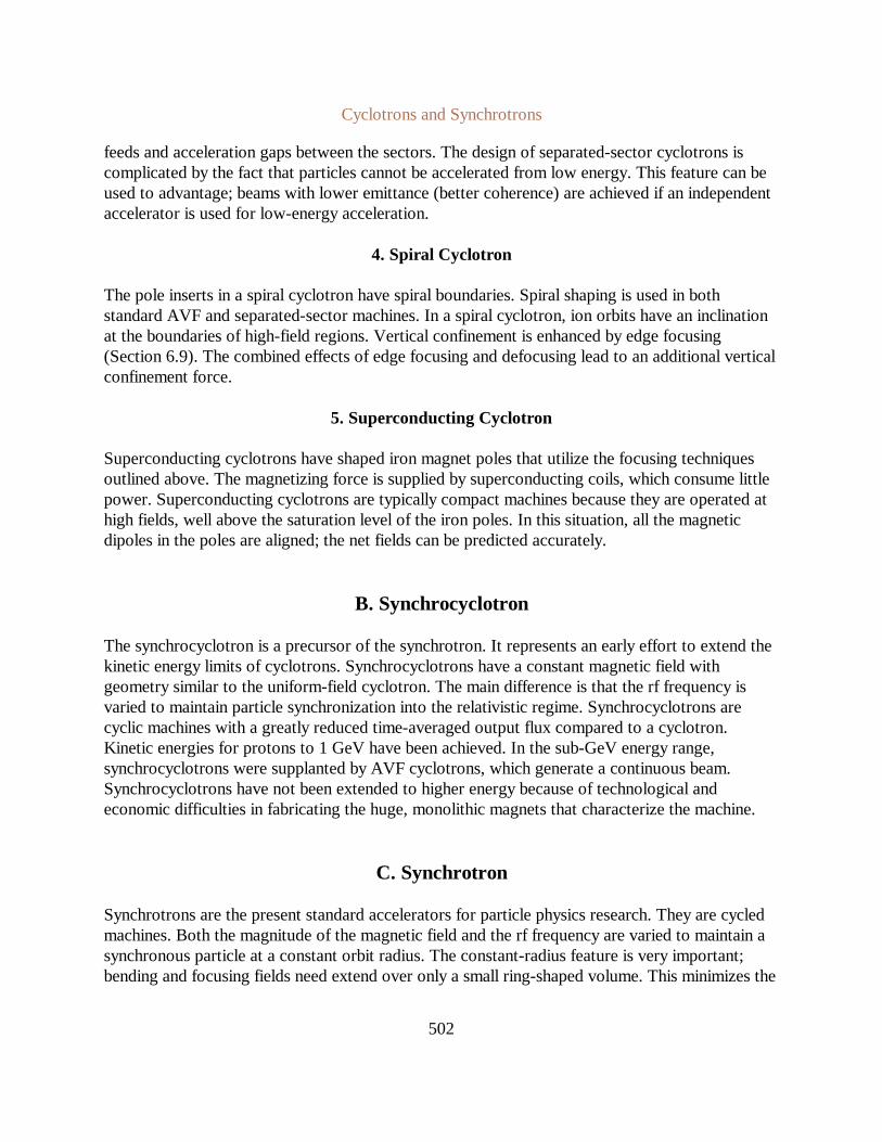
Cyclotrons and Synchrotrons
502
feeds and acceleration gaps between the sectors. The design of separated-sector cyclotrons iscomplicated by the fact that particles cannot be accelerated from low energy. This feature can beused to advantage; beams with lower emittance (better coherence) are achieved if an independentaccelerator is used for low-energy acceleration.
4. Spiral Cyclotron
The pole inserts in a spiral cyclotron have spiral boundaries. Spiral shaping is used in bothstandard AVF and separated-sector machines. In a spiral cyclotron, ion orbits have an inclinationat the boundaries of high-field regions. Vertical confinement is enhanced by edge focusing(Section 6.9). The combined effects of edge focusing and defocusing lead to an additional verticalconfinement force.
5. Superconducting Cyclotron
Superconducting cyclotrons have shaped iron magnet poles that utilize the focusing techniquesoutlined above. The magnetizing force is supplied by superconducting coils, which consume littlepower. Superconducting cyclotrons are typically compact machines because they are operated athigh fields, well above the saturation level of the iron poles. In this situation, all the magneticdipoles in the poles are aligned; the net fields can be predicted accurately.
B. Synchrocyclotron
The synchrocyclotron is a precursor of the synchrotron. It represents an early effort to extend thekinetic energy limits of cyclotrons. Synchrocyclotrons have a constant magnetic field withgeometry similar to the uniform-field cyclotron. The main difference is that the rf frequency isvaried to maintain particle synchronization into the relativistic regime. Synchrocyclotrons arecyclic machines with a greatly reduced time-averaged output flux compared to a cyclotron.Kinetic energies for protons to 1 GeV have been achieved. In the sub-GeV energy range,synchrocyclotrons were supplanted by AVF cyclotrons, which generate a continuous beam.Synchrocyclotrons have not been extended to higher energy because of technological andeconomic difficulties in fabricating the huge, monolithic magnets that characterize the machine.
C. Synchrotron
Synchrotrons are the present standard accelerators for particle physics research. They are cycledmachines. Both the magnitude of the magnetic field and the rf frequency are varied to maintain asynchronous particle at a constant orbit radius. The constant-radius feature is very important;bending and focusing fields need extend over only a small ring-shaped volume. This minimizes the

Cyclotrons and Synchrotrons
503
cost of the magnets, allowing construction of large-diameter machines for ion energies of up to800 GeV. Synchrotrons are used to accelerate both ions and electrons, although electronmachines are limited in energy by emission of synchrotron radiation. The main limits on achievableenergy for ions are the cost of the machine and availability of real estate. Cycling times are long inthe largest machines, typically many seconds. Electron synchrotrons and proton boosters cycle atfrequencies in the range of 15 to 60 Hz.
1. Weak Focusing Synchrotron
Early synchrotrons used weak focusing. The bending magnets were shaped to produce a field withindex in the range 0 <n < 1. With low focusing force, the combined effects of transverse particlevelocity and synchrotron oscillations (see Section 15.6) resulted in beams with large cross section.This implies costly, large-bore magnets.
2. Strong Focusing Synchrotron
All modern synchrotrons use transverse focusing systems composed of strong lenses in afocusing-defocusing array. Strong focusing minimizes the beam cross section, reducing themagnet size. Beam dynamics are more complex in a strong focusing synchrotron. The magnetsmust be constructed and aligned with high precision, and care must be taken to avoid resonanceinstabilities. Advances in magnet technology and beam theory have made it possible to overcomethese difficulties.
Alternating Gradient Synchrotron (AGS) . The bending field in an alternating gradientsynchrotron is produced by a ring of wedge-shaped magnets which fit together to form an annularregion of vertical field. The magnets have alternate positive and negative field gradient withn » 1.The combination of focusing and defocusing in the horizontal and vertical directions leads to netbeam confinement.
Separated Function Synchrotron. Most modern synchrotrons are configured as separatedfunction synchrotrons. The bending field is provided by sector magnets with uniform vertical field.Focusing is performed by quadrupole magnetic lens set between the bending magnets. Othermagnets may be included for correction of beam optics.
3. Storage Ring
A storage ring usually has the same focusing and bending field configuration as a separatedfunction synchrotron, but provides no acceleration. The magnetic fields are constant in time. Anrf cavity may be included for longitudinal beam manipulations such as stacking or, in the case of

Cyclotrons and Synchrotrons
504
electrons, maintaining kinetic energy in the presence of radiation loss. A storage ring containsenergetic particles at constant energy for long periods of time. The primary applications are forcolliding beam experiments and synchrotron radiation production.
4. Collider
A collider is a synchrotron, storage ring, dual synchrotron, or dual storage ring with specialgeometry to allow high-energy charged particles moving in opposite directions to collide head-onat a number of positions in the machine. The use of colliding beams significantly increases theamount of energy available to probe the structure of matter for elementary particle physics.Colliders have been operated (or are planned) for counter-rotating beams of protons (pp collider),electrons and positrons (e-e+), and protons and antiprotons (p ).p
Section 15.1 introduces the uniform-field cyclotron and the principles of circular resonantaccelerators. The longitudinal dynamics of the uniform-field cyclotron is reviewed in Section 15.2.The calculations deal with an interesting application of the phase equations when there is nosynchronous particle. The model leads to the choice of optimum acceleration history and tolimitson achievable kinetic energy. Sections 15.3 and 15.4 are concerned with AVF, or isochronous,cyclotrons. Transverse focusing is treated in the first section. Section 15.4 summarizesrelationships between magnetic field and rf frequency to preserve synchronization in fixed-field,fixed-frequency machines. There is also a description of the synchrocyclotron.
Sections 15.5-15.7 are devoted to the synchrotron. The first section describes general featuresof synchrotrons, including focusing systems, energy limits, synchrotron radiation, and thekinematics of colliding beams. The longitudinal dynamics of synchrotrons is the subject of Section15.6. Material includes constraints on magnetic field and rf frequency variation forsynchronization, synchrotron oscillations, and the transition energy. To conclude, Section 15.7summarizes the principles and benefits of strong focusing. Derivations are given to illustrate theeffects of alignment errors in a strong focusing system. Forbidden numbers of betatronwavelengths and mode coupling are discussed qualitatively.
15.1 PRINCIPLES OF THE UNIFORM-FIELD CYCLOTRON
The operation of the uniform-field cyclotron [E. 0. Lawrence, Science72, 376 (1930)] is based onthe fact that the gyrofrequency for non-relativistic ions [Eq. (3.39)] is independent of kineticenergy. Resonance between the orbital motion and an accelerating electric field can be achievedfor ion kinetic energy that is small compared to the rest energy. The configuration of theuniform-field cyclotron is illustrated in Figure 15.1a. Ions are constrained to circular orbits by a

Cyclotrons and Synchrotrons
505

Cyclotrons and Synchrotrons
506
fo qBo/2πmi (1.52×10⁷) Bo(tesla)/A, (15.1)
Tmax 48 (ZRB)2/A, (15.2)
vertical field between the poles of a magnet. The ions are accelerated in the gap between twoD-shaped metal structures (dees) located within the field region. An ac voltage is appliedto the dees by an rf resonator. The resonator is tuned to oscillate nearωg.
The acceleration history of an ion is indicated in Figure 15.1b. The acceleratorillustrated hasonly one dee excited by a bipolar waveform to facilitate extraction. A source, located at the centerof the machine continuously generates ions. The low-energy ions are accelerated to the oppositeelectrode during the positive-polarity half of the rf cycle. After crossing the gap, the ions areshielded from electric fields so that they follow a circular orbit. When the ions return to the gapafter a time interval they are again accelerated because the polarity of the dee voltage isπ/ωgoreversed. An aperture located at the entrance to the acceleration gaplimits ions to a small rangeof phase with respect to the rf field. If the ions were not limited to a small phase range, the outputbeam would have an unacceptably large energy spread. In subsequent gap crossings, the ionkinetic energy and gyroradius increase until the ions are extracted at the periphery of the magnet.The cyclotron is similar to the Wideröe linearaccelerator (Section 14.2); the increase in thegyroradius with energy is analogous to the increase in drift-tube length for the linear machine.
The rf frequency in cyclotrons is relatively low. The ion gyrofrequency is
whereA is the atomic mass number,mi/mp. Generally, frequency is in the range of 10 MHz formagnetic fields near 1 T. The maximum energy of ions in a cyclotron is limited by relativisticdetuning and radial variations of the magnetic field magnitude. In a uniform-field magnet field, thekinetic energy and orbit radius of non-relativistic ions are related by
whereTmax is given in MeV,R in meters, andB in tesla. For example, 30-MeV deuterons require a1-T field with good uniformity over a 1.25-m radius.
Transverse focusing in the uniform-field cyclotron is performed by an azimuthally symmetricvertical field with a radial gradient (Section 7.3). The main differences from the betatron are thatthe field index is small compared to unity ( and ) and that particle orbits extendνr 1 νz « 1over a wide range of radii. Figure 15.2 diagrams magnetic field in a typical uniform-field cyclotronmagnet and indicates the radial variation of field magnitude and field index,n. The field index isnot constant with radius. Symmetry requires that the field index be zero at the center of themagnet. It increases rapidly with radius at the edge of the pole. Cyclotron magnets are designedfor smalln over most of the field area to minimize desynchronization of particle orbits. Therefore,vertical focusing in a uniform-field cyclotron is weak.
There is no vertical magnetic focusing at the center of the magnet. By a fortunate coincidence,
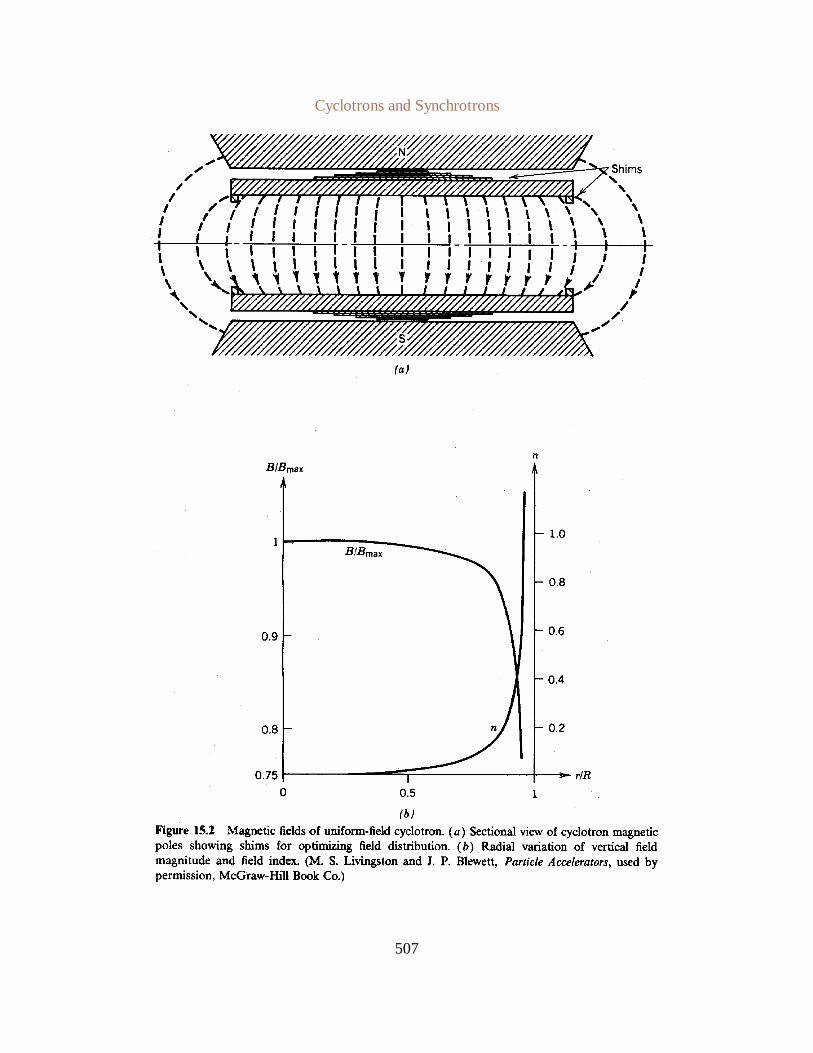
Cyclotrons and Synchrotrons
507

Cyclotrons and Synchrotrons
508
electrostatic focusing by the accelerating fields is effective for low-energy ions. The electric fieldpattern between the dees of a cyclotron act as the one-dimensional equivalent of the electrostaticimmersion lens discussed in Section 6.6. The main difference from the electrostatic lens is that iontransit-time effects can enhance or reduce focusing. For example, consider the portion of theaccelerating half-cycle when the electric field is rising. Ions are focused at the entrance side of thegap and defocused at the exit. When the transit time is comparable to the rf half-period, thetransverse electric field is stronger when the ions are near the exit, thereby reducing the netfocusing. The converse holds in the part of the accelerating half-cycle with falling field.
In order to extract ions from the machine at a specific location, deflection fields must beapplied. Deflection fields should affect only the maximum energy ions. Ordinarily, static electric(magnetic) fields in vacuum extend a distance comparable to the spacing between electrodes(poles) by the properties of the Laplace equation (Section 4.1). Shielding of other ions isaccomplished with a septum (separator), an electrode or pole that carries image charge or currentto localize deflection fields. An electrostatic septum is illustrated in Figure 15.3. A strong radialelectric field deflects maximum energy ions to a radius wheren > 1. Ions spiral out of the machine

Cyclotrons and Synchrotrons
509
∆R (R/2) (2qVo sinφs/T). (15.3)
V(t) Vo sinωt, (15.4)
along a well-defined trajectory. Clearly, a septum should not intercept a substantial fraction of thebeam. Septa are useful in the cyclotron because there is a relatively large separation betweenorbits. The separation for non-relativistic ions is
For example, with a peak dee voltageVo = 100 kV,φs = 60, R = 1 m, and T = 20 MeV, Eq.(15.3) implies that∆R = 0.44 cm.
15.2 LONGITUDINAL DYNAMICS OF THE UNIFORM-FIELDCYCLOTRON
In the uniform-field cyclotron, the oscillation frequency of gap voltage remains constant while theion gyrofrequency continually decreases. The reduction inωg with energy arises from two causes:(1) the relativistic increase in ion mass and (2) the reduction of magnetic field magnitude at largeradius. Models of longitudinal particle motion in a uniform-field cyclotron are similar to thosefor a traveling wave linear electron accelerator (Section 13.6); there is no synchronous phase. Inthis section, we shall develop equations to describe the phase history of ions in a uniform-fieldcyclotron. As in the electron linac, the behavior of a pulse of ions is found by following individualorbits rather than performing an orbit expansion about a synchronous particle. The model predictsthe maximum attainable energy and energy spread as a function of the phase width of the ionpulse. The latter quantity is determined by the geometry of the aperture illustrated in Figure 15.1.The model indicates strategies to maximize beam energy.The geometry of the calculation is illustrated in Figure 15.4. Assume that the voltage of dee1relative to dee2 is given by
whereω is the rf frequency. The following simplifying assumptions facilitate development of aphase equation:
1. Effects of the gap width are neglected. This is true when the gap width divided by theion velocity is small compared to 1/ω.
2. The magnetic field is radially uniform. The model is easily extended to include theeffects of field variations.
3. The ions circulate many times during the acceleraton cycle, so that it is sufficient toapproximate kinetic energy as a continuous variable and to identify the centroid of theparticle orbits with the symmetry axis of the machine.

Cyclotrons and Synchrotrons
510
φ ωt θ(t). (15.5)
dφ/dt ω dθ/dt ω ωg, (15.6)
ωg qBo/γmi qc2Bo/E. (15.7)
The phase of an ion at azimuthal positionθ and timet is defined as
Equation (15.5) is consistent with our previous definition of phase (Chapter 13). Particlescrossing the gap from deel to dee2 att = 0 haveφ = 0 and experience zero accelerating voltage.The derivative of Eq. (15.5) is
where
The quantityE in Eq. (15.7) is the total relativistic ion energy, . In the limit thatE T mic2
, the gyrofrequency is almost constant and Eq. (15.6) implies that particles haveT « mic2
constant phase during acceleration. Relativistic effects reduce the second term in Eq. (15.6). If therf frequency equals the non-relativistic gyrofrequency , then dφ/dt is always positive.ω ωgoThe limit of acceleration occurs whenφ reaches 180. In this circumstance, ions arrive at the gapwhen the accelerating voltage is zero; ions are trapped at a particular energy and circulate in thecyclotron at constant radius.

Cyclotrons and Synchrotrons
511
∆Em qVo sinφm. (15.8)
∆φ (dφ/dt) (π/ωg) π [(ωE/c2qBo) 1]. (15.9)
∆φ/∆E dφ/dE (π/qVo sinφ) [(ωE/c2qBo) 1]. (15.10)
sinφ dφ (π/qVo) [(ωE/c2qBo) 1] dE. (15.11)
cosφ cosφo (π/qVo) [(ω/2c2qBo) (E 2 Eo) (E Eo)], (15.12)
cosφ cosφo (π/qVo) (1 ω/ωgo) T (π/2qVomic2) (ω/ωgo) T 2. (15.13)
Equation (15.4), combined with the assumption of small gap width, implies that particlesmaking theirmth transit of the gap with phaseφm gain an energy.
In order to develop an analytic phase equation, it is assumed that energy increases continually andthat phase is a continuous function of energy,φ(E). The change of phase for a particle during thetransit through a dee is
Dividing Eq. (15.9) by Eq. (15.8) gives an approximate equation forφ(E):
Equation (15.10) can be rewritten
Integration of Eq. (15.11) gives an equation for phase as a function of particle energy:
whereφo is the injection phase. The cyclotron phase equation is usually expressed in terms of thekinetic energy T. Taking and , Eq. (15.12) becomesT E m2
oc ωgo qBo/mi
During acceleration, ion phase may traverse the range . The content of Eq.0 < φ < 180(15.13) can be visualized with the help of Figure 15.5. The quantity cosφ is plotted versusT withφo as a parameter. The curves are parabolas. In Figure 15.5a, the magnetic field is adjusted so that
. The maximum kinetic energy is defined by the intersection of the curve with cosφ = - 1.ω ωoThe best strategy is to inject the particles in a narrow range nearφo = 0. Clearly, higher kineticenergy can be obtained if (Fig. 15.5b). The particle is injected withφo > 0. It initiallyω < ωogains on the rf field phase and then lags. A particle phase history is valid only if cosφ remainsbetween -1 and +1. In Figure 15.5b, the orbit withφo = 45 is not consistent with acceleration tohigh energy. The curve forφo = 90 leads to a higher final energy thanφo = 135.
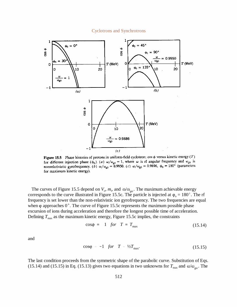
Cyclotrons and Synchrotrons
512
cosφ 1 for T Tmax (15.14)
cosφ 1 for T ½Tmax. (15.15)
The curves of Figure 15.5 depend onVo, mi, and . The maximum achievable energyω/ωgocorresponds to the curve illustrated in Figure 15.5c. The particle is injected atφo = 180. The rffrequency is set lower than the non-relativistic ion gyrofrequency. The two frequencies are equalwhenφ approaches 0. The curve of Figure 15.5c represents the maximum possible phaseexcursion of ions during acceleration and therefore the longest possible time of acceleration.Defining Tmax as the maximum kinetic energy, Figure 15.5c implies, the constraints
and
The last condition proceeds from the symmetric shape of the parabolic curve. Substitution of Eqs.(15.14) and (15.15) in Eq. (15.13) gives two equations in two unknowns forTmax and . Theω/ωgo

Cyclotrons and Synchrotrons
513
ω/ωgo 1/(1 Tmax/2mic2) (15.16)
Tmax 16qVomic2/π. (15.17)
solution is
and
Equation (15.17) is a good approximation when .T « mic2
Note that the final kinetic energy is maximized by takingVo large. This comes about because ahigh gap voltage accelerates particles in fewer revolutions so that there is less opportunity forparticles to get out of synchronization. Typical acceleration gap voltages are ±100 kV. Inspectionof Eq. (15.17) indicates that the maximum kinetic energy attainable is quite small comparedto mic
2. In a typical cyclotron, the relativistic mass increase amounts to less than 2%. The smallrelativistic effects are important because they accumulate over many particle revolutions.
To illustrate typical parameters, consideracceleration of deuterium ions. The rest energy is 1.9GeV. If Vo = 100 kV, Eq. (15.17) implies thatTmax = 31 MeV. The peak energy will be lower ifradial variations of magnetic field are included. WithBo = 1.5 T, the non-relativisticgyrofrequency isfo = 13.6 MHz. For peak kinetic energy, the rf frequency should be about 13.5MHz. The ions make approximately 500 revolutions during acceleration.
15.3 FOCUSING BY AZIMUTHALLY VARYING FIELDS (AVF)
Inspection of Eqs. (15.6) and (15.7) shows that synchronization in a cyclotron can be preservedonly if the average bending magnetic field increases with radius. A positive field gradientcorresponds to a negative field index in a magnetic field with azimuthal symmetry, leading tovertical defocusing. A positive field index can be tolerated if there is an extra source of verticalfocusing. One way to provide additional focusing is to introduce azimuthal variations in thebending field. In this section, we shall study particle orbits in azimuthally varying fields. The intentis to achieve a physical understanding of AVF focusing through simple models. The actual designof accelerators with AVF focusing [K.R. Symon,et. al., Phys. Rev.103, 1837 (1956); F.T. Cole,et .al., Rev. Sci. Instrum.28, 403 (1957)] is carried out using complex analytic calculations and,inevitably, numerical solution of particle orbits. The results of this section will be applied toisochronous cyclotrons in Section 15.4. In principle, azimuthally varying fields could be used forfocusing in accelerators with constant particle orbit radius, such as synchrotrons or betatrons.These configurations are usually referred to as FFAG (fixed-field, alternating-gradient)accelerators. In practice, the cost of magnets in FFAG machines is considerably higher than moreconventional approaches, so AVF focusing is presently limited to cyclotrons.
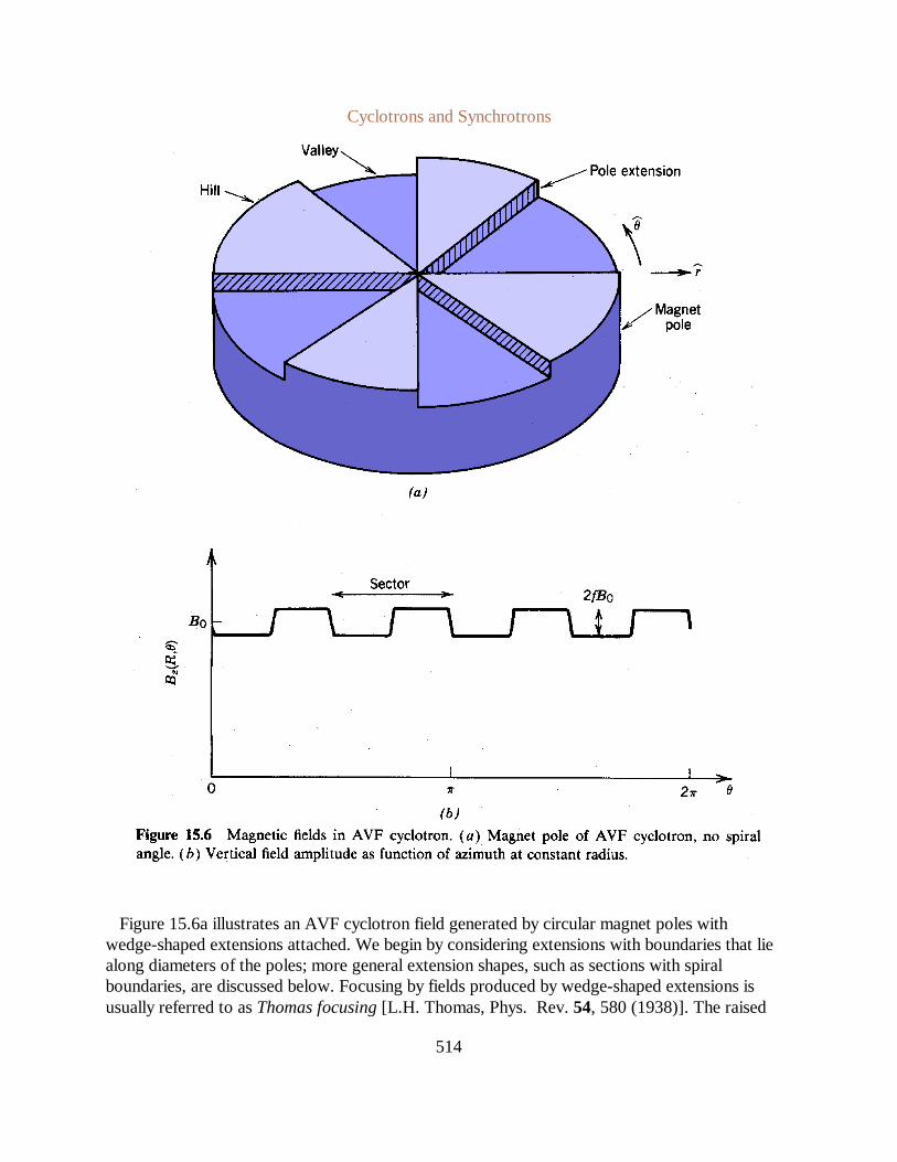
Cyclotrons and Synchrotrons
514
Figure 15.6a illustrates an AVF cyclotron field generated by circular magnet poles withwedge-shaped extensions attached. We begin by considering extensions with boundaries that liealong diameters of the poles; more general extension shapes, such as sections with spiralboundaries, are discussed below. Focusing by fields produced by wedge-shaped extensions isusually referred to asThomas focusing[L.H. Thomas, Phys. Rev.54, 580 (1938)]. The raised
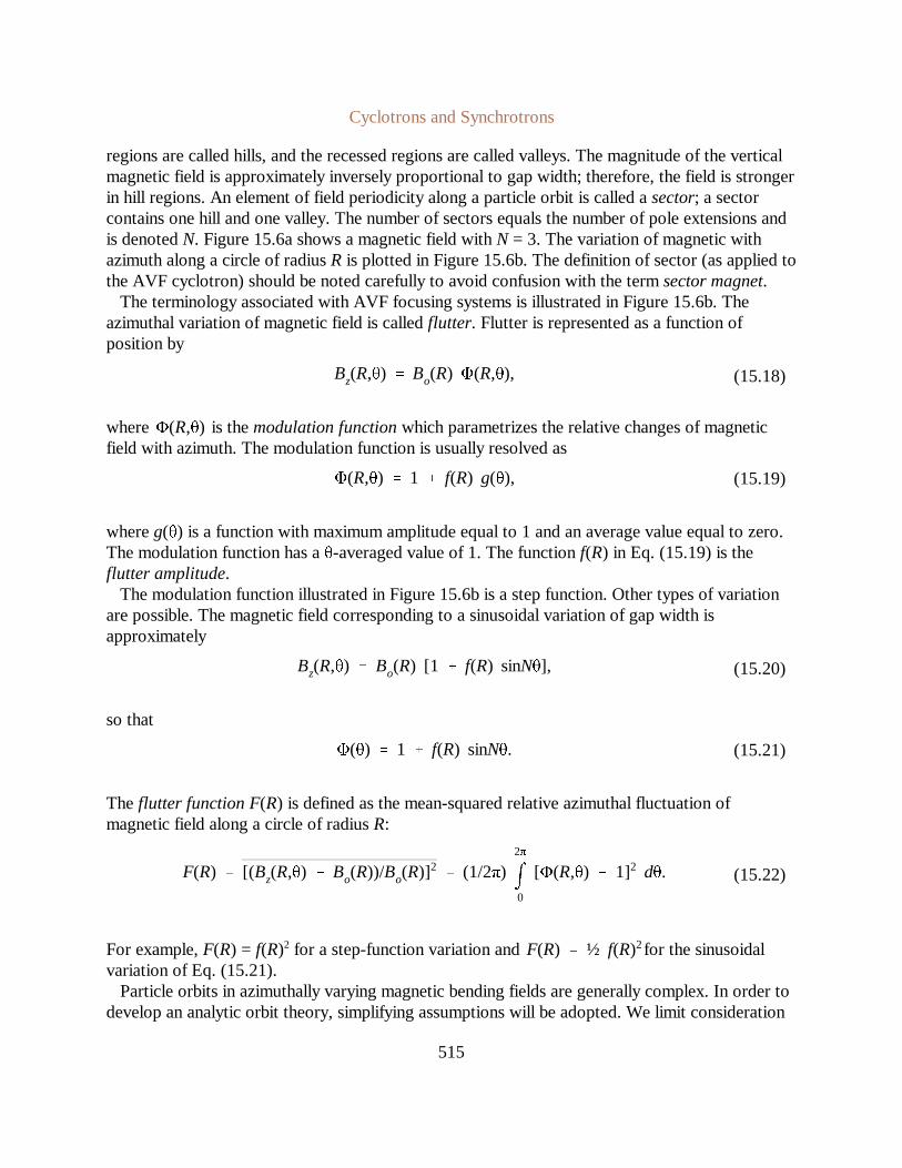
Cyclotrons and Synchrotrons
515
Bz(R,θ) Bo(R) Φ(R,θ), (15.18)
Φ(R,θ) 1 f(R) g(θ), (15.19)
Bz(R,θ) Bo(R) [1 f(R) sinNθ], (15.20)
Φ(θ) 1 f(R) sinNθ. (15.21)
F(R) [(Bz(R,θ) Bo(R))/Bo(R)]2 (1/2π)
2π
0
[Φ(R,θ) 1]2 dθ. (15.22)
regions are called hills, and the recessed regions are called valleys. The magnitude of the verticalmagnetic field is approximately inversely proportional to gap width; therefore, the field is strongerin hill regions. An element of field periodicity along a particle orbit is called asector; a sectorcontains one hill and one valley. The number of sectors equals the number of pole extensions andis denotedN. Figure 15.6a shows a magnetic field withN = 3. The variation of magnetic withazimuth along a circle of radiusR is plotted in Figure 15.6b. The definition of sector (as applied tothe AVF cyclotron) should be noted carefully to avoid confusion with the termsector magnet.
The terminology associated with AVF focusing systems is illustrated in Figure 15.6b. Theazimuthal variation of magnetic field is calledflutter. Flutter is represented as a function ofposition by
where is themodulation functionwhich parametrizes the relative changes of magneticΦ(R,θ)field with azimuth. The modulation function is usually resolved as
whereg(θ) is a function with maximum amplitude equal to 1 and an average value equal to zero.The modulation function has aθ-averaged value of 1. The functionf(R) in Eq. (15.19) is theflutter amplitude.
The modulation function illustrated in Figure 15.6b is a step function. Other types of variationare possible. The magnetic field corresponding to a sinusoidal variation of gap width isapproximately
so that
The flutter function F(R) is defined as the mean-squared relative azimuthal fluctuation ofmagnetic field along a circle of radiusR:
For example,F(R) = f(R)2 for a step-function variation and for the sinusoidalF(R) ½ f(R)2
variation of Eq. (15.21).Particle orbits in azimuthally varying magnetic bending fields are generally complex. In order to
develop an analytic orbit theory, simplifying assumptions will be adopted. We limit consideration
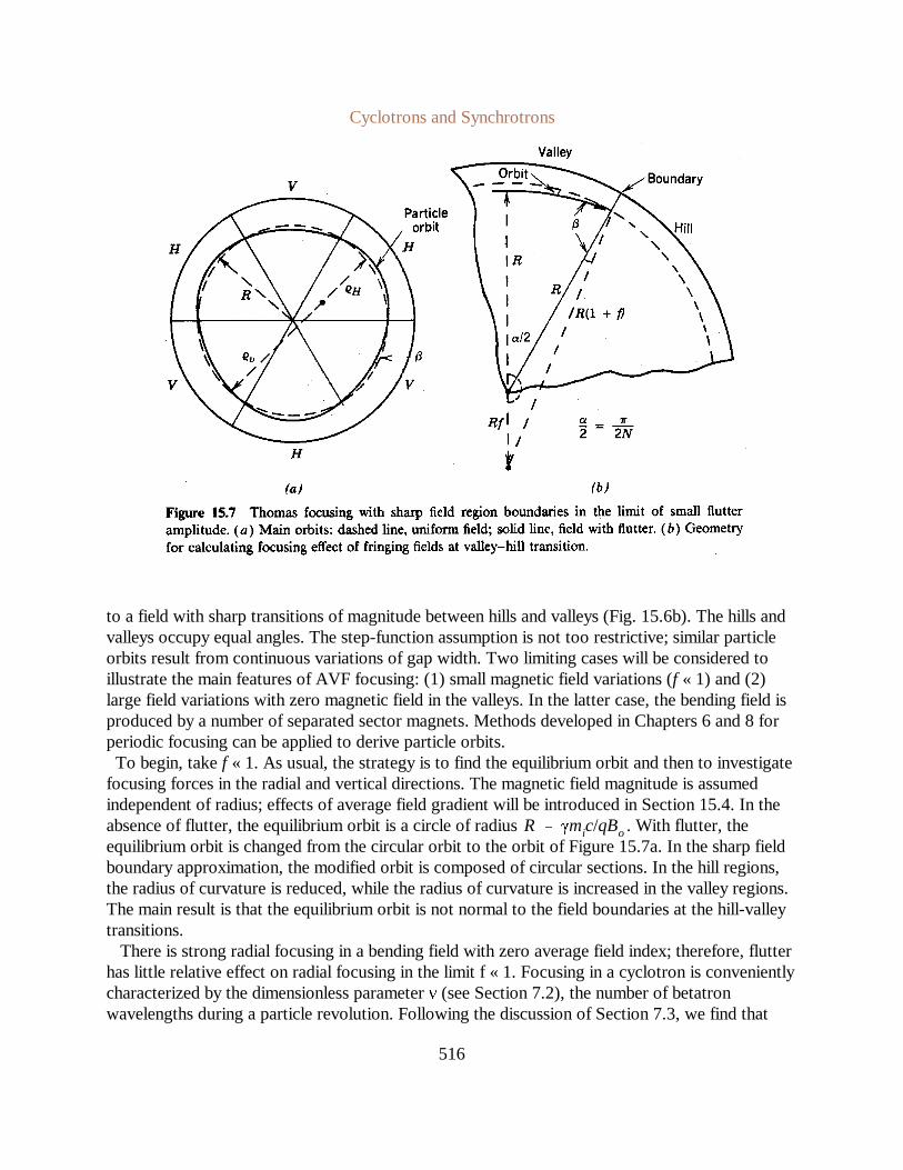
Cyclotrons and Synchrotrons
516
to a field with sharp transitions of magnitude between hills and valleys (Fig. 15.6b). The hills andvalleys occupy equal angles. The step-function assumption is not too restrictive; similar particleorbits result from continuous variations of gap width. Two limiting cases will be considered toillustrate the main features of AVF focusing: (1) small magnetic field variations (f « 1) and (2)large field variations with zero magnetic field in the valleys. In the latter case, the bending field isproduced by a number of separated sector magnets. Methods developed in Chapters 6 and 8 forperiodic focusing can be applied to derive particle orbits.
To begin, takef « 1. As usual, the strategy is to find the equilibrium orbit and then to investigatefocusing forces in the radial and vertical directions. The magnetic field magnitude is assumedindependent of radius; effects of average field gradient will be introduced in Section 15.4. In theabsence of flutter, the equilibrium orbit is a circle of radius . With flutter, theR γmic/qBoequilibrium orbit is changed from the circular orbit to the orbit of Figure 15.7a. In the sharp fieldboundary approximation, the modified orbit is composed of circular sections. In the hill regions,the radius of curvature is reduced, while the radius of curvature is increased in the valley regions.The main result is that the equilibrium orbit is not normal to the field boundaries at the hill-valleytransitions.
There is strong radial focusing in a bending field with zero average field index; therefore, flutterhas little relative effect on radial focusing in the limit f « 1. Focusing in a cyclotron is convenientlycharacterized by the dimensionless parameterν (see Section 7.2), the number of betatronwavelengths during a particle revolution. Following the discussion of Section 7.3, we find that

Cyclotrons and Synchrotrons
517
ν2r 1 (15.23)
focal length (γmic/q[2Bof]) / |tanβ| R/2f |tanβ|, (15.24)
Ab 1 0
2f tanβ/R 1(15.25)
|β| πf/2N, (15.26)
Ab 1 0
πf 2/NR 1(15.26)
Ad 1 πR/N
0 1(15.26)
for a radially uniform average field magnitude.In contrast, flutter plays an important part in vertical focusing. Inspection of Figure 15.7a shows
that the equilibrium orbit crosses between hill and valley regions at an angle to the boundary. Thevertical forces acting on the particle are similar to those encountered in edge focusing (Section6.9). The field can be resolved into a uniform magnetic field of magnitudeBo[l - f (R)]superimposed on fields of magnitude 2Bof(R) in the hill regions. Comparing Figure 15.7a toFigure 6.20, the orbit is inclined so that there is focusing at both the entrance and exit of a hillregion. The vertical force arises from the fringing fields at the boundary; the horizontal fieldcomponents are proportional to the change in magnetic field, 2Bof(R). Following Eq. 6.30, theboundary fields act as a thin lens with positive focal length
whereβ is the angle of inclination of the orbit to the boundary. The ray transfer matrixcorresponding to transit across a boundary is
The inclination angle can be evaluated from the geometric construction of Figure 15.7b. Theequilibrium orbit crosses the boundary at aboutr = R. The orbit radii of curvature in the hill andvalley regions areR(1 ± f). To first order, the inclination angle is
whereN is the number of sectors. The ray transfer matrix for a boundary is expressed as
for smallβ. Neglecting variations in the orbit length through hills and valleys caused by the flutter,the transfer matrix for drift is
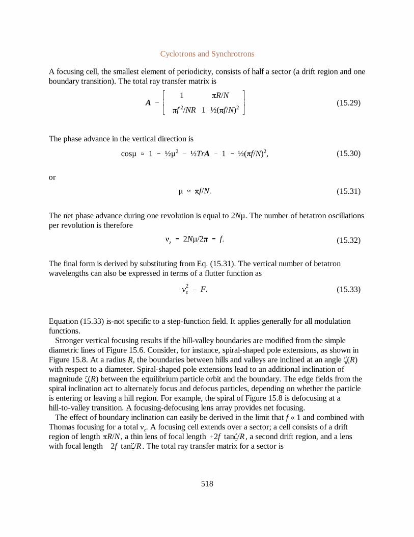
Cyclotrons and Synchrotrons
518
A
1 πR/N
πf 2/NR 1½(πf/N)2(15.29)
cosµ 1 ½µ2 ½TrA 1 ½(πf/N)2, (15.30)
µ πf/N. (15.31)
νz 2Nµ/2π f. (15.32)
ν2z F. (15.33)
A focusing cell, the smallest element of periodicity, consists of half a sector (a drift region and oneboundary transition). The total ray transfer matrix is
The phase advance in the vertical direction is
or
The net phase advance during one revolution is equal to 2Nµ. The number of betatron oscillationsper revolution is therefore
The final form is derived by substituting from Eq. (15.31). The vertical number of betatronwavelengths can also be expressed in terms of a flutter function as
Equation (15.33) is-not specific to a step-function field. It applies generally for all modulationfunctions.
Stronger vertical focusing results if the hill-valley boundaries are modified from the simplediametric lines of Figure 15.6. Consider, for instance, spiral-shaped pole extensions, as shown inFigure 15.8. At a radiusR, the boundaries between hills and valleys are inclined at an angleζ(R)with respect to a diameter. Spiral-shaped pole extensions lead to an additional inclination ofmagnitudeζ(R) between the equilibrium particle orbit and the boundary. The edge fields from thespiral inclination act to alternately focus and defocus particles, depending on whether the particleis entering or leaving a hill region. For example, the spiral of Figure 15.8 is defocusing at ahill-to-valley transition. A focusing-defocusing lens array provides net focusing.
The effect of boundary inclination can easily be derived in the limit thatf « 1 and combined withThomas focusing for a totalνz. A focusing cell extends over a sector; a cell consists of a driftregion of length , a thin lens of focal length , a second drift region, and a lensπR/N 2f tanζ/Rwith focal length . The total ray transfer matrix for a sector is2f tanζ/R
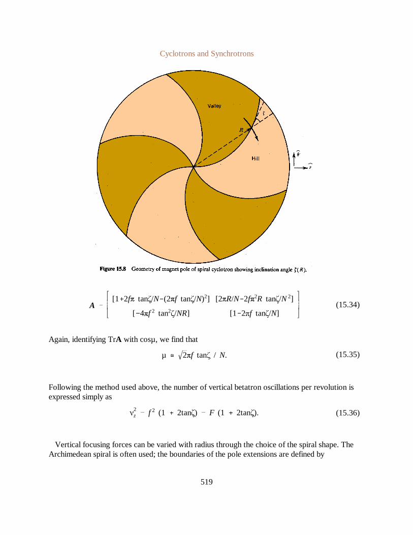
Cyclotrons and Synchrotrons
519
A
[12fπ tanζ/N(2πf tanζ/N)2] [2πR/N2fπ2R tanζ/N2]
[4πf 2 tan2ζ/NR] [12πf tanζ/N](15.34)
µ 2πf tanζ / N. (15.35)
ν2z f 2 (1 2tanζ) F (1 2tanζ). (15.36)
Again, identifying TrA with cosµ, we find that
Following the method used above, the number of vertical betatron oscillations per revolution isexpressed simply as
Vertical focusing forces can be varied with radius through the choice of the spiral shape. TheArchimedean spiral is often used; the boundaries of the pole extensions are defined by
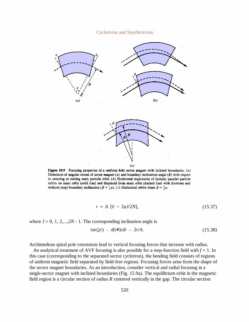
Cyclotrons and Synchrotrons
520
r A [θ 2πJ/2N], (15.37)
tanζ(r) d(rθ)/dr 2r/A. (15.38)
where J = 0, 1, 2,...,2N - 1. The corresponding inclination angle is
Archimedean spiral pole extensions lead to vertical focusing forces that increase with radius.An analytical treatment of AVF focusing is also possible for a step-function field withf = 1. In
this case (corresponding to the separated sector cyclotron), the bending field consists of regionsof uniform magnetic field separated by field-free regions. Focusing forces arise from the shape ofthe sector magnet boundaries. As an introduction, consider vertical and radial focusing in asingle-sector magnet with inclined boundaries (Fig. 15.9a). The equilibrium orbit in the magneticfield region is a circular section of radiusR centered vertically in the gap. The circular section

Cyclotrons and Synchrotrons
521
β ½α (15.39)
ν2z (1 2 tanζ) (15.40)
ν2r 2 tanζ. (15.41)
subtends an angleα. Assume that the boundary inclinations,β, are equal at the entrance and exitof the magnet.
In the vertical direction, the ray transfer matrix for the magnet is the product of matricesrepresenting edge focusing at the entrance, a drift distanceαR, and focusing at the exit. We canapply Eqs. (15.27) and (15.28) to calculate the total ray transfer matrix. In order to calculatefocusing in the radial direction, we must include the effect of the missing sector field introducedby the inclination angle P. For the geometry of Figure 15.9a, the inclination reduces radialfocusing in the sector magnet. Orbits with and without a boundary inclination are plotted inFigure 15.9b. Figure 15.9c shows the equilibrium particle orbit and an off-axis parallel orbit in asector magnet with . The boundary is parallel to a line through the midplane of theβ ½α
magnet; the gyrocenters of both orbits also lie on this line. Therefore, the orbits are parallelthroughout the sector and there is no focusing. A value of inclination moves theβ < ½α
gyrocenter of the off-axis particle to the left; the particle emerges from the sector focused towardthe axis. The limit on for radial focusing in a uniform-field sector magnet is
We now turn our attention to the AVF sector field with diametric boundaries shown in Figure15.10. The equilibrium orbits can be constructed with compass and straightedge. The orbits arecircles in the sector magnets and straight lines in between. They must match in position and angleat the boundaries. Figures 15.10a, b show solutions withN = 2 andN = 3 for hills and valleysoccupying equal azimuths ( ). Note that in all cases the inclination angle of the orbit at aα π/Nboundary is one-half the angular extent of the sector, . Figures 15.10c and d illustrate theβ ½α
geometric construction of off-axis horizontal orbits for conditions corresponding to stability( ) and instability ( ). The case ofN = 2 is unstable for allα > π/N,β < ½α α < π/N,β > ½α
choices ofα. This arises because particles are overfocused when . This effect is clearlyα > π/Nvisible in Figure 15.10e. It is generally true that particle orbits are unstable in any type of AVFfield with N = 2.
Spiral boundaries may also be utilized in separated sector fields. Depending on whether theparticles are entering or leaving a sector, the edge-focusing effects are either focusing ordefocusing in the vertical direction. Applying matrix algebra and the results of Section 6.9, it iseasy to show thatνz is
for . Spiral boundaries contribute alternate focusing and defocusing forces in the radialα π/Ndirection that are 180 out of phase with the axial forces. For , the number of radialα π/Nbetatron oscillations per revolution is approximately

Cyclotrons and Synchrotrons
522
Cyclotrons and Synchrotrons
523
15.4 THE SYNCHROCYCLOTRON AND THE AVF CYCLOTRON
Following the success of the uniform-field cyclotron, efforts were made to reach higher beamkinetic energy. Two descendants of the cyclotron are the synchrocyclotron and the AVF(isochronous) cyclotron. The machines resolve the problem of detuning between particlerevolutions and rf field in quite different ways. Synchrocyclotrons have the same geometry as theSF cyclotron. A large magnet with circular poles produces an azimuthally symmetric vertical fieldwith positive field index. Ions are accelerated from rest to high energy by an oscillating voltageapplied between dees. The main difference is that the frequency is varied to preserve synchronism.
There are a number of differences in the operation of synchrocyclotrons and cyclotrons.Synchrocyclotrons are cycled, rather than continuous; therefore, the time-average beam current ismuch lower. The longitudinal dynamics of particles in a synchrocyclotron do not follow the modelof Section 15.2 because there is a synchronous phase. The models for phase dynamics developedin Chapter 13 can be adapted to the synchrocyclotron. The machine can contain a number ofconfined particle bunches with phase parameters centered about the bunch that has ideal matchingto the rf frequency. The beam bunches are distributed as a group of closely spaced turns ofslightly different energy. The acceptance of the rf buckets decreases moving away from the idealmatch, defining a range of time over which particles can be injected into the machine. In researchapplications, the number of bunches contained in the machine in a cycle is constrained by theallowed energy spread of the output beam.
There are technological limits on the rate at which the frequency of oscillators cpn be swept.These limits were particularly severe in early synchrocyclotrons that used movable mechanicaltuners rather than the ferrite tuners common on modern synchrotrons. The result is that theacceleration cycle of a synchrocyclotron extends over a longer period than the acceleration timefor an ion in a cyclotron. Typically, ions perform between 10,000 and 50,000 revolutions duringacceleration in a synchrocyclotron. The high recirculation factor implies lower voltage betweenthe dees. The cycled operation of the synchrocyclotron leads to different methods of beamextraction compared to cyclotrons. The low dee voltage implies that orbits have small separation(< 1 mm), ruling out the use of a septum. On the other hand, all turns can be extracted at the sametime by a pulsed field because they are closely spaced in radius. Figure 15.11illustrates onemethod of beam extraction from a synchrocyclotron. A pulsed electric field is used to deflect ionson to a perturbed orbit which leads them to a magnetic shield. The risetime of voltage on thekicker electrodes should be short compared to the revolution time of ions. Pulsed extraction ischaracteristic of cycled machines like the synchrocyclotron and synchrotron. In large synchrotronswith relatively long revolution time, pulsed magnets with ferrite cores are used for beamdeflection.
Containment of high-energy ions requires large magnets. For example, a 600-MeV proton has agyroradius of 2.4 m in a 1.5-T field. This implies a pole diameter greater than 15 ft.Synchro-cyclotron magnets are among the largest monolithic, iron core magnets ever built. Thelimitation of this approach is evident; the volume of iron required rises roughly as the cube of thekinetic energy. Two synchrocyclotrons are still in operation: the 184-in. machine at LawrenceBerkeley Laboratory and the CERN SC.
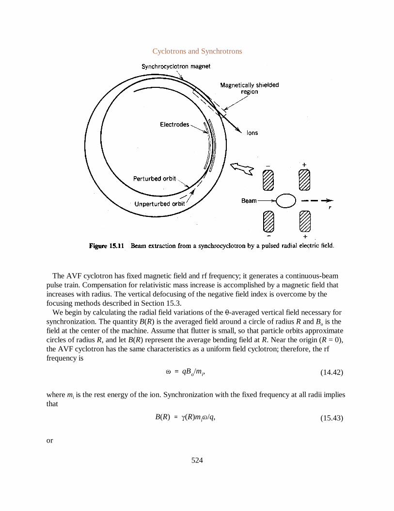
Cyclotrons and Synchrotrons
524
ω qBo/mi, (14.42)
B(R) γ(R)miω/q, (15.43)
The AVF cyclotron has fixed magnetic field and rf frequency; it generates a continuous-beampulse train. Compensation for relativistic mass increase is accomplished by a magnetic field thatincreases with radius. The vertical defocusing of the negative field index is overcome by thefocusing methods described in Section 15.3.
We begin by calculating the radial field variations of theθ-averaged vertical field necessary forsynchronization. The quantityB(R) is the averaged field around a circle of radiusR andBo is thefield at the center of the machine. Assume that flutter is small, so that particle orbits approximatecircles of radiusR, and letB(R) represent the average bending field atR. Near the origin (R = 0),the AVF cyclotron has the same characteristics as a uniform field cyclotron; therefore, the rffrequency is
wheremi is the rest energy of the ion. Synchronization with the fixed frequency at all radii impliesthat
or

Cyclotrons and Synchrotrons
525
B(R)/Bo γ(R). (15.44)
R
γ(R) βmic
qB(R)
mic
qB(R)γ21
mic
qBo
γ21γ
. (15.45)
B(R)/Bo γ(R) 1 (qBoR/mic2)2 . (15.46)
n(R) [R/B(R)] [dB(R)/dR] (γ21). (15.47)
The average magnetic field is also related to the average orbit radius and ion energy through Eq.(3.38):
Combining Eqs. (15.44) and (15.45), we find
Equation (15.46) gives the following radial variation of the field index:
Two methods for generating a bending field with negative field index (positive radial gradient) areillustrated in Figure 15.12. In the first, the distance between poles decreases as a function of
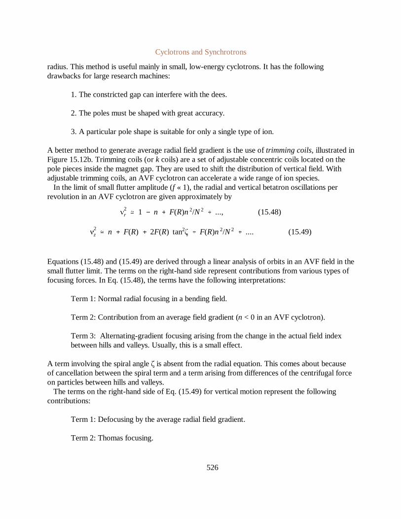
Cyclotrons and Synchrotrons
526
ν2r 1 n F(R)n 2/N2
..., (15.48)
ν2z n F(R) 2F(R) tan2ζ F(R)n 2/N2
.... (15.49)
radius. This method is useful mainly in small, low-energy cyclotrons. It has the followingdrawbacks for large research machines:
1. The constricted gap can interfere with the dees.
2. The poles must be shaped with great accuracy.
3. A particular pole shape is suitable for only a single type of ion.
A better method to generate average radial field gradient is the use oftrimming coils, illustrated inFigure 15.12b. Trimming coils (ork coils) are a set of adjustable concentric coils located on thepole pieces inside the magnet gap. They are used to shift the distribution of vertical field. Withadjustable trimming coils, an AVF cyclotron canaccelerate a wide range of ion species.
In the limit of small flutter amplitude (f « 1), the radial and vertical betatron oscillations perrevolution in an AVF cyclotron are given approximately by
Equations (15.48) and (15.49) are derived through a linear analysis of orbits in an AVF field in thesmall flutter limit. The terms on the right-hand side represent contributions from various types offocusing forces. In Eq. (15.48), the terms have the following interpretations:
Term 1: Normal radial focusing in a bending field.
Term 2: Contribution from an average field gradient (n < 0 in an AVF cyclotron).
Term 3: Alternating-gradient focusing arising from the change in the actual field indexbetween hills and valleys. Usually, this is a small effect.
A term involving the spiral angleζ is absent from the radial equation. This comes about becauseof cancellation between the spiral term and a term arising from differences of the centrifugal forceon particles between hills and valleys.
The terms on the right-hand side of Eq. (15.49) for vertical motion represent the followingcontributions:
Term 1: Defocusing by the average radial field gradient.
Term 2: Thomas focusing.

Cyclotrons and Synchrotrons
527
νr γ (15.50)
Term 3: FD focusing by the edge fields of a spiral boundary.
Term 4: Same as the third term of Eq. (15.48).
Symmetry considerations dictate that the field index and spiral angle near the center of an AVFcyclotron approach zero. The flutter amplitude also approaches zero at the center because theeffects of hills and valleys on the field cancel out at radii comparable to or less than the gap widthbetween poles. As in the conventional cyclotron, electrostatic focusing at the acceleraton gapsplays an important role for vertical focusing of low-energy ions. At large radius, there is littleproblem in ensuring good radial focusing. Neglecting the third term, Eq. (15.48) may be rewrittenas
using Eq. (15.47). The quantityνr is always greater than unity; radial focusing is strong.Regarding vertical focusing, the combination of Thomas focusing and spiral focusing in Eq.(15.49) must increase with radius to compensate for the increase in field index. This can beaccomplished by a radial increase ofF(R) or ζ(R). In the latter case, boundary curves withincreasingζ (such as the Archimedean spiral) can be used. Isochronous cyclotrons have theproperty that the revolution time is independent of the energy history of the ions. Therefore, thereare no phase oscillations, and ions have neutral stability with respect to the rf phase. The magnetpoles of high-energy isochronous cyclotrons must be designed with high accuracy so that particlesynchronization is maintained through the acceleration process.
In addition to high-energy applications, AVF cyclotrons are well suited to low-energy medicaland industrial applications. The increased vertical focusing compared to a simple gradient fieldmeans that the accelerator has greater transverse acceptance. Higher beam currents can becontained, and the machine is more tolerant to field errors (see Section 15.7). Phase stability ishelpful, even in low-energy machines. The existence of a synchronous phase implies higherlongitudinal acceptance and lower beam energy spread. The AVF cyclotron is much lessexpensive per ion produced than a uniform-field cyclotron.
In the range of kinetic energy above 100 MeV, the separated sector cyclotron is a better choicethan the single-magnet AVF cyclotron. The separated sector cyclotron consists of three or morebending magnets separated by field-free regions. It has the following advantages:
1. Radio-frequency cavities for beam acceleration can be located between the sectorsrather than between the magnet poles. This allows greater latitude in designing thefocusing magnetic field and the acceleration system. Multiple acceleration gaps can beaccommodated, leading to rapid acceleration and large orbit separation.
2. The bending field is produced by a number of modular magnets rather than a singlelarger unit. Modular construction reduces the problems of fabrication and mechanicalstress. This is particularly important at high energy.

Cyclotrons and Synchrotrons
528
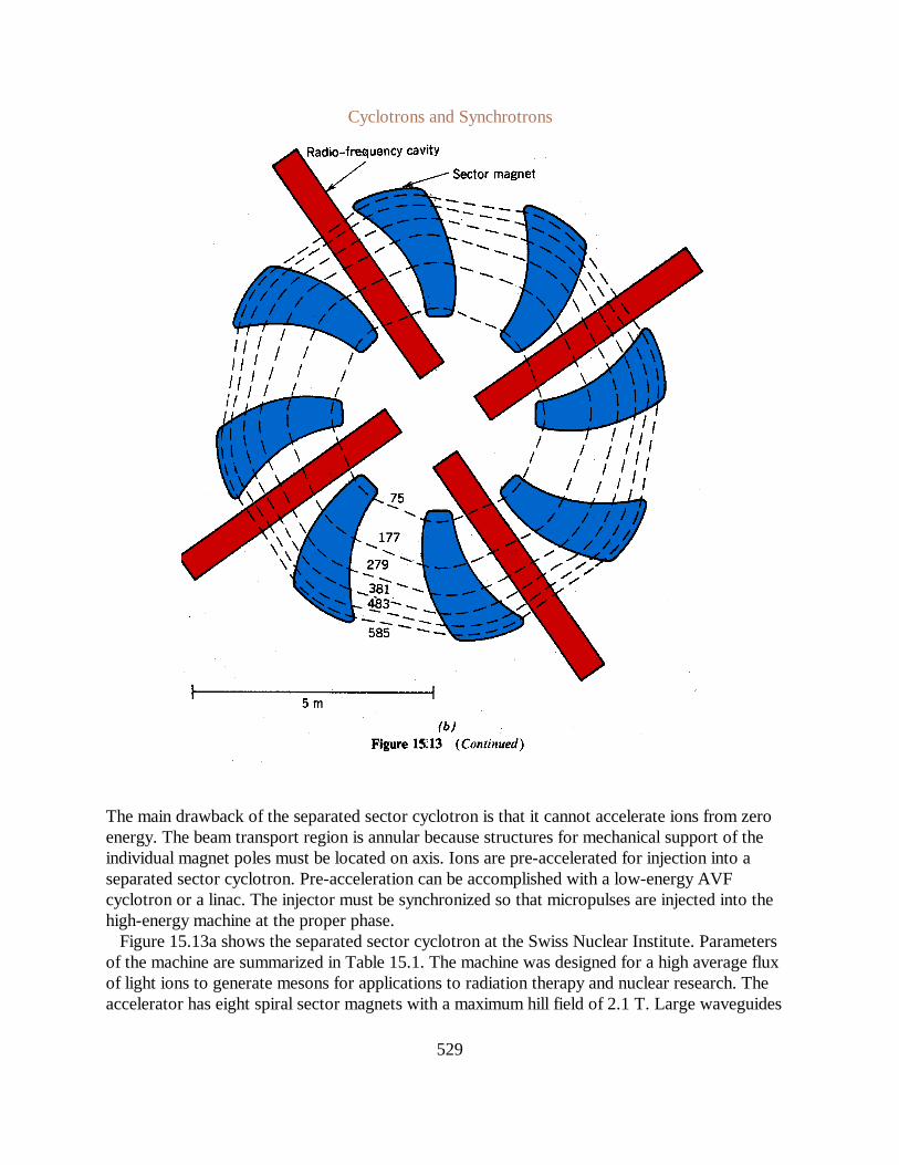
Cyclotrons and Synchrotrons
529
The main drawback of the separated sector cyclotron is that it cannot accelerate ions from zeroenergy. The beam transport region is annular because structures for mechanical support of theindividual magnet poles must be located on axis. Ions are pre-accelerated for injection into aseparated sector cyclotron. Pre-acceleration can be accomplished with a low-energy AVFcyclotron or a linac. The injector must be synchronized so that micropulses are injected into thehigh-energy machine at the proper phase.
Figure 15.13a shows the separated sector cyclotron at the Swiss Nuclear Institute. Parametersof the machine are summarized in Table 15.1. The machine was designed for a high average fluxof light ions to generate mesons for applications to radiation therapy and nuclear research. Theaccelerator has eight spiral sector magnets with a maximum hill field of 2.1 T. Large waveguides
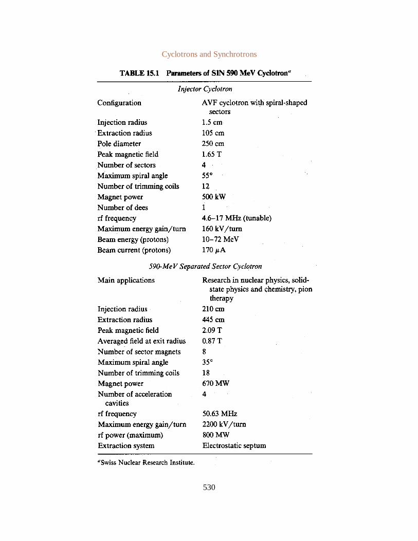
Cyclotrons and Synchrotrons
530

Cyclotrons and Synchrotrons
531
connect rf supplies to a four acceleration gaps. In operation, the machine requires 0.5 MW of rfinput power. The peak acceleration gap voltage is 500 kV. The maximum orbit diameter of thecyclotron is 9 in for a maximum output energy of 590 MeV (protons). The time-averaged beamcurrent is 200 µA. A standard AVF cyclotron with four spiral-shaped sectors is used as aninjector. An increase of average beam current to 1 mA is expected with the addition of a newinjector. The injector is a spiral cyclotron with four sectors. The injector operates at 50.7 MHzand generates 72-MeV protons. Figure 15.13b is an overhead view of the magnets and rf cavitiesin the separated sector cyclotron. Six selected orbits are illustrated at equal energy intervals from72 to 590 MeV. Note that the distance an ion travels through the sector field increases with orbitradius (negative effective field index). The diagram also indicates the radial increase of theinclination angle between sector field boundaries and the particle orbits.
15.5 PRINCIPLES OF TliE SYNCHROTRON
Synchrotrons are resonant circular particle accelerators in which both the magnitude of thebending magnetic field and the rf frequency are cycled. An additional feature of most modemsynchrotrons is that focusing forces are adjustable independent of the bending field. Independentvariation of the focusing forces, beam-bending field, and rf frequency gives synchrotrons twocapabilities that lead to beam energies far higher than those from other types of circularaccelerators:
1. The betatron wavelength of particles can be maintained constant as acceleration proceeds. Thismakes it possible to avoid the orbital resonances that limit the output energy of the AVFcyclotron.
2. The magnetic field amplitude is varied to preserve a constant particle orbit radius duringacceleration. Therefore, the bending field need extend over only a small annulus rather than fill acomplete circle. This implies large savings in the cost of the accelerator magnets. Furthermore,the magnets can be fabricated as modules and assembled into ring accelerators exceeding 6 kmin circumference.
The main problems of the synchrotron are (1) a complex operation cycle and (2) low average flux.The components of a modem separated function synchrotron are illustrated in Figure 15.14. An
ultra-high-vacuum chamber for beam transport forms a closed loop. Circular sections may beinterrupted by straight sections to facilitate beam injection, beam extraction, and experiments.Acceleration takes place in a cavity filled with ferrite cores to provide inductive iso a over abroad frequency range. The cavity is similar to a linear inductionaccelerator cavity. The twodifferences are (1) an ac voltage is applied across the gap and (2) the ferrites are not driven tosaturation to minimize power loss.
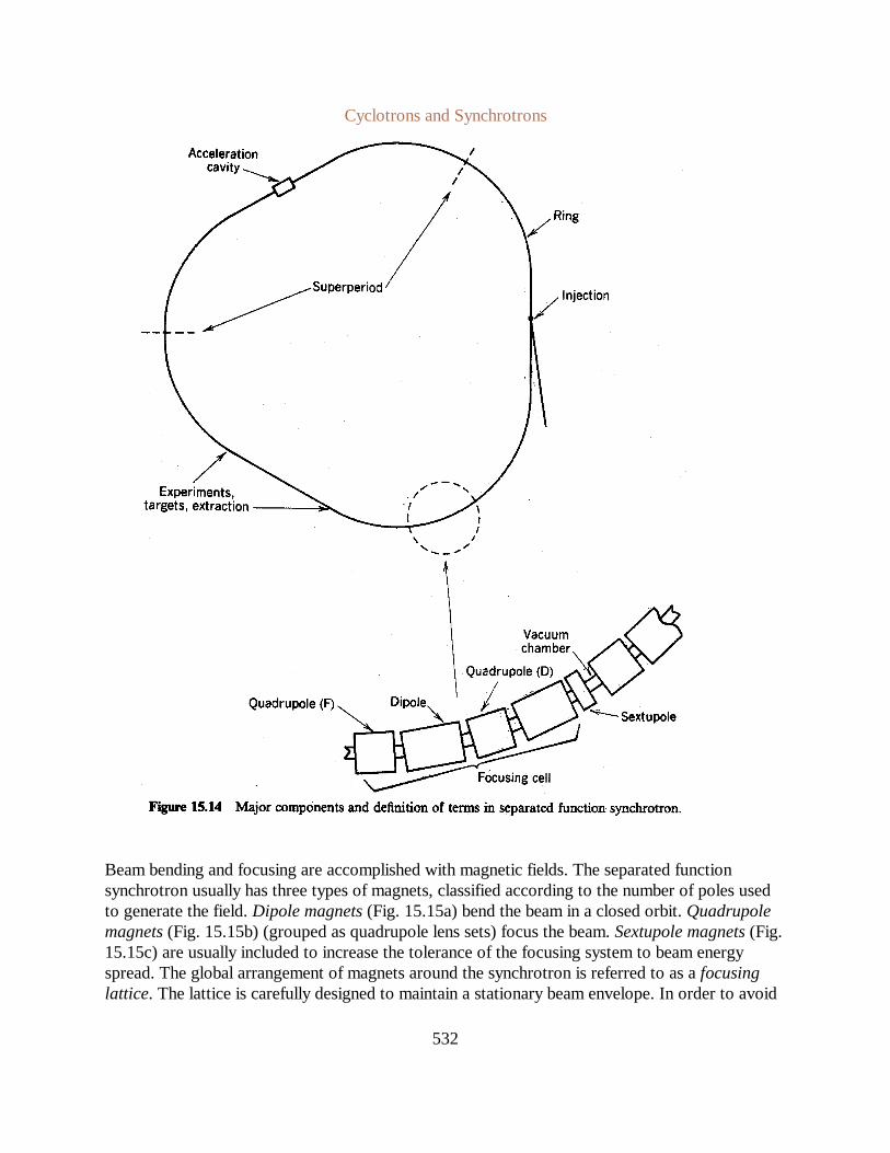
Cyclotrons and Synchrotrons
532
Beam bending and focusing are accomplished with magnetic fields. The separated functionsynchrotron usually has three types of magnets, classified according to the number of poles usedto generate the field.Dipole magnets(Fig. 15.15a) bend the beam in a closed orbit.Quadrupolemagnets(Fig. 15.15b) (grouped as quadrupole lens sets) focus the beam.Sextupole magnets(Fig.15.15c) are usually included to increase the tolerance of the focusing system to beam energyspread. The global arrangement of magnets around the synchrotron is referred to as afocusinglattice. The lattice is carefully designed to maintain a stationary beam envelope. In order to avoid

Cyclotrons and Synchrotrons
533
resonance instabilities, the lattice design must not allow betatron wavelengths to equal acharacteristic dimension of the machine (such as the circumference). Resonance conditions areparametrized in terms offorbidden valuesof νr andνz.
A focusing cell is strictly defined as the smallest element of periodicity in a focusing system.A period of a noncircular synchrotron contains a large number of optical elements. A cell mayencompass a curved section, a straight section, focusing and bending magnets, and transitionelements between the sections. The termsuperperiodis usually used to designate the minimumperiodic division of a synchrotron, while focusing cell is applied to a local element of periodicitywithin a superperiod. The most common local cell configuration is theFODO cell. It consists of afocusing quadrupole (relative to ther or z direction), a dipole magnet, a defocusing quadrupole,and another dipole. Horizontal focusing forces in the bending magnets are small compared to thatin the quadrupoles. For transverse focusing, the cell is represented as a series of focusing anddefocusing lenses separated. by drift (open) spaces.
The alternating-gradient synchrotron (AGS) is the precursor of the separated functionsynchrotron. The AGS has a ring of magnets which combine the functions of beam bending andfocusing. Cross sections of AGS magnets are illustrated in Figure 15.16. A strong positive or

Cyclotrons and Synchrotrons
534
negative radial gradient is superimposed on the bending field; horizontal and vertical focusingarises from the transverse fields associated with the gradient (Section 7.3). The magnet ofFigure 15.16a gives strong radial focusing and horizontal defocusing, while the opposite holds forthe magnet of Figure 15.16b.
Early synchrotrons utilized simple gradient focusing in an azimuthally symmetric field. Theywere constructed from a number of adjacent bending magnets with uniform field index in therange 0 <n < 1. These machines are now referred to asweak focusing synchrotronsbecause thebetatron wavelength of particles was larger than the machine circumference. The zero-gradientsynchrotron (ZGS) (Fig. 15.16c) was an interesting variant of the weak focusing machine.Bending and focusing were performed by sector magnets with uniform-field magnitude (zerogradient). The sector field boundaries were inclined with respect to the orbits to give verticalfocusing [via edge focusing (Section 6.9)] and horizontal focusing [via sector focusing (Section6.8)]. The advantage of the ZGS compared to other weak focusing machines was that higherbending fields could be achieved without local saturation of the poles.

Cyclotrons and Synchrotrons
535
R 3.3E/B (m), (15.51)
P 2cE4ro/3R2(moc2)3 (watts), (15.52)
ro q 2/4πεomoc2. (15.53)
re 2.82 × 10¹⁵ m. (15.54)
P cVo/2πR. (15.55)
E [3Vo(moc2)3R/4πro]
0.25. (15.56)
The limit on kinetic energy in an ion synchrotron is set by the bending magnetic field magnitudeand the area available for the machine. The ring radius of relativistic protons is given by
where is the average magnetic field (in tesla) andE is the total ion energy in GeV. Most ionBsynchrotrons accelerate protons; protons have the highest charge-to-mass ratio and reach thehighest kinetic energy per nucleon for a given magnetic field. Synchrotrons have been used forheavy-ion acceleration. In this application, ions are pre-accelerated in a linear accelerator anddirected through a thin foil to strip electrons. Only ions with high charge states are selected forinjection into the synchrotron.
The maximum energy in an electron synchrotron is set by emission ofsynchrotron radiation.Synchrotron radiation results from the continuous transverse acceleration of particles in a circularorbit. The total power emitted per particle is
whereE is the total particle energy andR is the radius of the circle. Power in Eq. (15.52) is givenin electron volts per second if all energies on the right-hand side are expressed in electron volts.The quantityro is the classical radius of the particle,
The classical radius of the electron is
Inspection of Eqs. (15.52) and (15.53) shows that synchrotron radiation has a negligible effectin ion accelerators. Compared to electrons, the power loss is reduced by a factor of . To(me/mi)
4
illustrate the significance of synchrotron radiation in electronaccelerators, consider a synchrotronin which electrons gain an energyeVo per turn. The power input to electrons (in eV/s) is
Setting Eqs. (15.52) and (15.55) equal, the maximum allowed total energy is
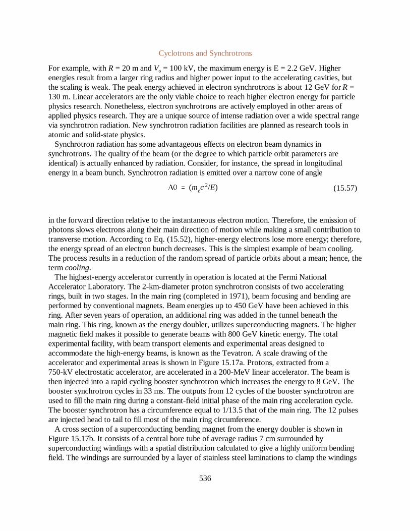
Cyclotrons and Synchrotrons
536
∆θ (mec2/E) (15.57)
For example, withR = 20 m andVo = 100 kV, the maximum energy is E = 2.2 GeV. Higherenergies result from a larger ring radius and higher power input to the accelerating cavities, butthe scaling is weak. The peak energy achieved in electron synchrotrons is about 12 GeV forR =130 m. Linear accelerators are the only viable choice to reach higher electron energy for particlephysics research. Nonetheless, electron synchrotrons are actively employed in other areas ofapplied physics research. They are a unique source of intense radiation over a wide spectral rangevia synchrotron radiation. New synchrotron radiation facilities are planned as research tools inatomic and solid-state physics.
Synchrotron radiation has some advantageous effects on electron beam dynamics insynchrotrons. The quality of the beam (or the degree to which particle orbit parameters areidentical) is actually enhanced by radiation. Consider, for instance, the spread in longitudinalenergy in a beam bunch. Synchrotron radiation is emitted over a narrow cone of angle
in the forward direction relative to the instantaneous electron motion. Therefore, the emission ofphotons slows electrons along their main direction of motion while making a small contribution totransverse motion. According to Eq. (15.52), higher-energy electrons lose more energy; therefore,the energy spread of an electron bunch decreases. This is the simplest example of beam cooling.The process results in a reduction of the random spread of particle orbits about a mean; hence, thetermcooling.
The highest-energy accelerator currently in operation is located at the Fermi NationalAccelerator Laboratory. The 2-km-diameter proton synchrotron consists of two acceleratingrings, built in two stages. In the main ring (completed in 1971), beam focusing and bending areperformed by conventional magnets. Beam energies up to 450 GeV have been achieved in thisring. After seven years of operation, an additional ring was added in the tunnel beneath themain ring. This ring, known as the energy doubler, utilizes superconducting magnets. The highermagnetic field makes it possible to generate beams with 800 GeV kinetic energy. The totalexperimental facility, with beam transport elements and experimental areas designed toaccommodate the high-energy beams, is known as the Tevatron. A scale drawing of theaccelerator and experimental areas is shown in Figure 15.17a. Protons, extracted from a750-kV electrostatic accelerator, are accelerated in a 200-MeV linear accelerator. The beam isthen injected into a rapid cycling booster synchrotron which increases the energy to 8 GeV. Thebooster synchrotron cycles in 33 ms. The outputs from 12 cycles of the booster synchrotron areused to fill the main ring during a constant-field initial phase of the main ring acceleration cycle.The booster synchrotron has a circumference equal to 1/13.5 that of the main ring. The 12 pulsesare injected head to tail to fill most of the main ring circumference.
A cross section of a superconducting bending magnet from the energy doubler is shown inFigure 15.17b. It consists of a central bore tube of average radius 7 cm surrounded bysuperconducting windings with a spatial distribution calculated to give a highly uniform bendingfield. The windings are surrounded by a layer of stainless steel laminations to clamp the windings

Cyclotrons and Synchrotrons
537
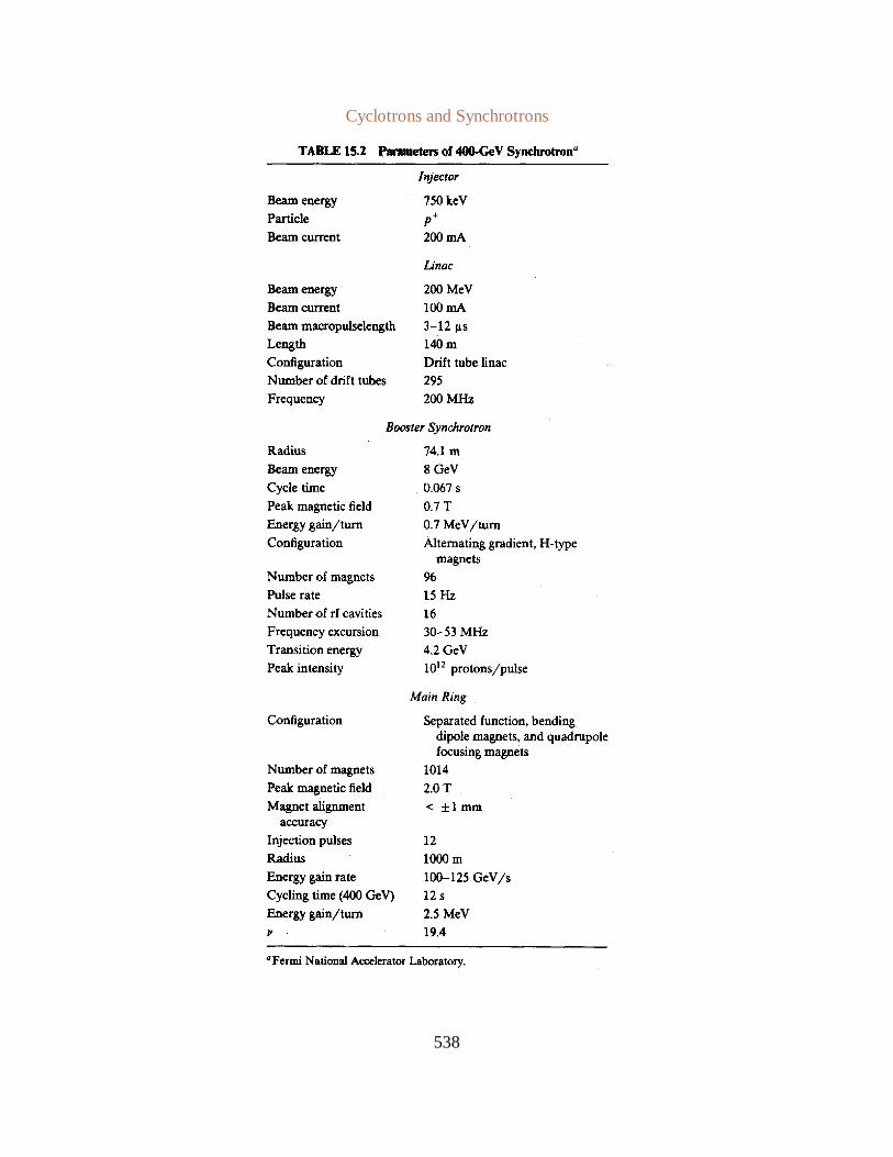
Cyclotrons and Synchrotrons
538
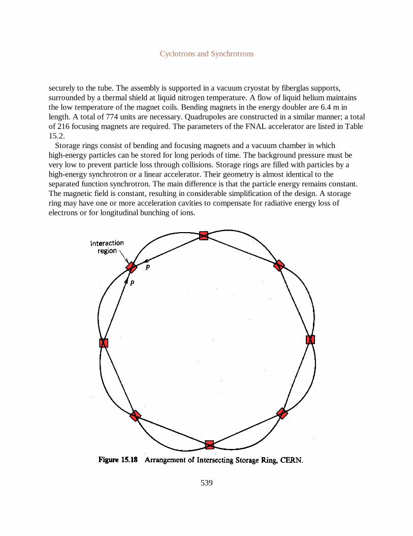
Cyclotrons and Synchrotrons
539
securely to the tube. The assembly is supported in a vacuum cryostat by fiberglas supports,surrounded by a thermal shield at liquid nitrogen temperature. A flow of liquid helium maintainsthe low temperature of the magnet coils. Bending magnets in the energy doubler are 6.4 m inlength. A total of 774 units are necessary. Quadrupoles are constructed in a similar manner; a totalof 216 focusing magnets are required. The parameters of the FNAL accelerator are listed in Table15.2.
Storage rings consist of bending and focusing magnets and a vacuum chamber in whichhigh-energy particles can be stored for long periods of time. The background pressure must bevery low to prevent particle loss through collisions. Storage rings are filled with particles by ahigh-energy synchrotron or a linear accelerator. Their geometry is almost identical to theseparated function synchrotron. The main difference is that the particle energy remains constant.The magnetic field is constant, resulting in considerable simplification of the design. A storagering may have one or more acceleration cavities to compensate for radiative energy loss ofelectrons or for longitudinal bunching of ions.

Cyclotrons and Synchrotrons
540
cβ1 c (β1 βi) / (1 βuβ1). (15.59)
cβ2 cβu, (15.58)
One of the main applications of storage rings is in colliding beam facilities for high-energy particlephysics. A geometry used in the ISR (intersecting storage ring) at CERN is shown in Figure15.18. Two storage rings with straight and curved sections are interleaved. Proton beamscirculating in opposite directions intersect at small angles at eight points of the ring.Proton-proton interactions are studied by detectors located near the intersection points.
Colliding beams have a significant advantage for high-energy physics research. The mainrequisite for probing the nature of elementary particles is that a large amount of energy must beavailable to drive reactions with a high threshold. When a moving beam strikes a stationary target(Fig. 15.19a), the kinetic energy of the incident particle is used inefficiently. Conservation ofmomentum dictates that a large portion of the energy is transformed to kinetic energy of thereaction products. The maximum energy available to drive a reaction in Figure 15.19a can becalculated by a transformation to the center-of-momentum (CM) frame. In the CM frame, theincident and target particles move toward one another with equal and opposite momenta. Thereaction products need not have kinetic energy to conserve momentum when viewed in the CMframe; therefore, all the initial kinetic energy is available for the reaction.
For simplicity, assume that the rest mass of the incident particle is equal to that of the targetparticle. Assume the CM frame moves at a velocitycβu relative to the stationary frame. Using Eq.(2.30), the velocity of the target particle in the CM frame is given by
and the transformed velocity of the incident particle is
Both particles have the same value ofγ’ in the CM frame; the condition of equal and oppositemomenta implies

Cyclotrons and Synchrotrons
541
β
2 β
1. (15.60)
βu (1/β1) (1/β21) 1. (15.61)
T (γ11) moc2, (15.62)
Tcm 2 (γ11) moc2, (15.63)
γ1 1/ 1β21, γ
1 1/ 1β2u.
Combining Eqs. (15.58), (15.59), and (15.60), we find that
Equation (15.61) allows us to compare the energy invested in the incident particle,
to the maximum energy available for particle reactions,
where

Cyclotrons and Synchrotrons
542
Tcm 2 (γ11) moc2. (15.63)
Table 15.3 showsTcm/T as a function ofγ1, along with equivalent kinetic energy values forprotons. In the non-relativistic range, half the energy is available. The fraction drops off at highkinetic energy. Increasing the kinetic energy of particles striking a stationary target givesdiminishing returns. The situation is much more favorable in an intersecting storage ring. Thestationary frame is the CM frame. The CM energy available from ring particles withγ1 is

Cyclotrons and Synchrotrons
543
For example, a 21-GeV proton accelerator operated in conjunction with an intersecting storagering can investigate the same reactions as a 1000-GeV accelerator with a stationary target. Theprice to pay for this advantage is reduction in the number of measurable events for physicsexperiments. A stationary target is usually at solid density. The density of a stored beam ismore than 10 orders of magnitude lower. A major concern in intersecting storage rings isluminosity, a measure of beam density in physical space and velocity space. Given avelocity-dependent cross section, the luminosity determines the reaction rate between the beams.The required luminosity depends on the cross section of the reaction and the nature of the eventdetectors.
A list of accelerators and storage rings with the most energetic beams is given in Table 15.4.The energy figure is the kinetic energy measured in the accelerator frame. The history ofaccelerators for particle physics during the last 50 years has been one of an exponential increase inthe available CM energy. Although this is attributable in part to an increase in the size ofequipment, the main reason for the dramatic improvement has been the introduction of newacceleration techniques. When a particular technology reached the knee of its growth curve, anew type of accelerator was developed. For example, proton accelerators evolved fromelectrostatic machines to cyclotrons. The energy energy limit of cyclotrons was resolved bysynchrocyclotrons which lead to the weak focusing synchrotron. The development of strongfocusing made the construction of large synchrotrons possible. Subsequently, colliding beamtechniques brought about a substantial increase in CM energy from existing machines. Atpresent, there is considerable activity in converting the largest synchrotrons to colliding beamfacilities.
In the continuing quest for high-energy proton beams for elementary particle research, the nextstated goal is to reach a proton kinetic energy of 20 TeV (20 × 1012 eV). At present, the onlyidentified technique to achieve such an extrapolation is to build an extremely large machine. A20-TeV synchrotron with conventional magnets operating at an average field of I T has a radiusof 66 km and a circumference of 414 km. The power requirements of conventional magnets insuch a large machine are prohibitive; superconducting magnets are essential. Superconductingmagnets can be designed in two ranges. Superconducting coils can be combined with aconventional pole assembly for fields below saturation. Because superconducting coils sustain afield with little power input, there is also the option for high-field magnets with completelysaturated poles. A machine with 6-T magnets has a circumference of 70 km.
Studies have recently been carried out for a superconducting super collider (SSC) [see, M.Tigner, Ed.,Accelerator Physics Issues for a Superconducting Super Collider, University ofMichigan, UM HE 84-1, 1984]. This machine is envisioned as two interleaved 20-TeV protonsynchrotrons with counter-rotating beams and a number of beam intersection regions. Estimatesof the circumference of the machine range from 90 to 160 km, depending on details of the magnetdesign. The CM energy is a factor of 40 higher than that attainable in existing accelerators. If it isconstructed, the SSC may mark the termination point of accelerator technology in terms ofparticle energy; it is difficult to imagine a larger machine. Considerations of cost versus rewards inbuilding the SSC raise interesting questions about economic limits to our knowledge of the

Cyclotrons and Synchrotrons
544
γ2t
δp/ps
δS/S, (15.64)
universe.
15.6 LONGITUDINAL DYNAMICS OF SYNCHROTRONS
The description of longitudinal particle motion in synchrotrons has two unique aspects comparedto synchrocyclotrons and AVF cyclotrons. The features arise from the geometry of the machineand the high energy of the particles:
1. Variations of longitudinal energy associated with stable phase confinement of particlesin an rf bucket result in horizontal particle oscillations. The synchrotron oscillations sumwith the usual betatron oscillations that arise from spreads in transverse velocity.Synchrotron oscillations must be taken intoaccount in choosing the size of thegood fieldregion of focusing magnets.
2. The range of stable synchronous phase in a synchrotron depends on the energy ofparticles. This effect is easily understood. At energies comparable to or less thanmoc
2,particles are non-relativistic; therefore, their velocity depends on energy. In this regime,low-energy particles in a beam bunch take a longer time to complete a circuit of theaccelerator and return to the acceleration cavity. Therefore, the accelerating voltage mustrise with time atφs for phasestability ( ). At relativistic energies, particle velocity is almost independent of0 < φs < π/2energy; the particle orbit circumference is the main determinant of the revolution time.Low-energy particles have smaller orbit radii and therefore take less time to return to theacceleration gap. In this case, the range of stable phase is . The energy thatπ/2 < φs < π
divides the regimes is called thetransition energy. In synchrotrons that bridge thetransition energy, it isessential to shift the phase of the rf field before the bunched structure of the beam is lost.This effect is unimportant in electron synchrotrons because electrons are always injectedabove the transition energy.
Models are developed in this section to describe the longitudinal dynamics of particles insynchrotrons. We begin by introducing the quantityγt, the transition gamma factor. The parametercharacterizes the dependence of particle orbit radius in the focusing lattice to changes inmomentum. We shall see thatγt corresponds to the relativistic mass factor at the transition energy.After calculating examples ofγt in different focusing systems, we shall investigate the equilibriumconditions that define a synchronous phase. The final step is to calculate longitudinal oscillationsabout the synchronous particle.
The transition gamma factor is defined by
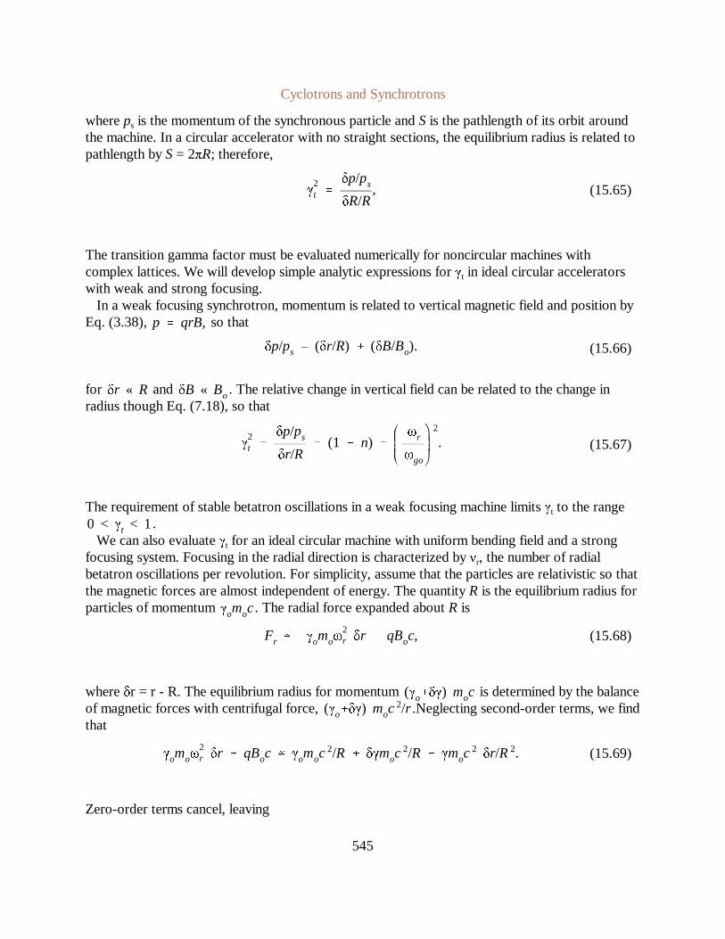
Cyclotrons and Synchrotrons
545
γ2t
δp/ps
δR/R, (15.65)
δp/ps (δr/R) (δB/Bo). (15.66)
γ2t
δp/ps
δr/R (1 n)
ωr
ωgo
2
. (15.67)
Fr γomoω2r δr qBoc, (15.68)
γomoω2r δr qBoc γomoc
2/R δγmoc2/R γmoc
2 δr/R2. (15.69)
whereps is the momentum of the synchronous particle andS is the pathlength of its orbit aroundthe machine. In a circular accelerator with no straight sections, the equilibrium radius is related topathlength byS= 2πR; therefore,
The transition gamma factor must be evaluated numerically for noncircular machines withcomplex lattices. We will develop simple analytic expressions forγt in ideal circular acceleratorswith weak and strong focusing.
In a weak focusing synchrotron, momentum is related to vertical magnetic field and position byEq. (3.38), so thatp qrB,
for and . The relative change in vertical field can be related to the change inδr « R δB « Boradius though Eq. (7.18), so that
The requirement of stable betatron oscillations in a weak focusing machine limitsγt to the range.0 < γt < 1
We can also evaluateγt for an ideal circular machine with uniform bending field and a strongfocusing system. Focusing in the radial direction is characterized byνr, the number of radialbetatron oscillations per revolution. For simplicity, assume that the particles are relativistic so thatthe magnetic forces are almost independent of energy. The quantityR is the equilibrium radius forparticles of momentum . The radial force expanded aboutR isγomoc
whereδr = r - R. The equilibrium radius for momentum is determined by the balance(γoδγ) mocof magnetic forces with centrifugal force, .Neglecting second-order terms, we find(γoδγ) moc
2/rthat
Zero-order terms cancel, leaving
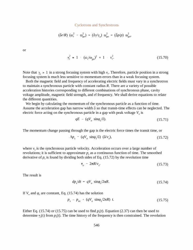
Cyclotrons and Synchrotrons
546
(δr/R) (ω2r ω
2go) (δγ/γo) ω
2go (δp/p) ω
2go,
γ2t 1 (ωr/ωgo)
2 1 ν
2r . (15.70)
qE (qVo sinφs/δ). (15.71)
∆ps (qVo sinφs/δ) (δ/vs), (15.72)
τo 2πR/vs. (15.73)
dps/dt qVo sinφs/2πR. (15.74)
ps pso (qVo sinφs/2πR) t. (15.75)
or
Note that in a strong focusing system with highνr. Therefore, particle position in a strongγt » 1focusing system is much less sensitive to momentum errors than in a weak focusing system.
Both the magnetic field and frequency of accelerating electric fields must vary in a synchrotronto maintain a synchronous particle with constant radiusR. There are a variety of possibleacceleration histories corresponding to different combinations of synchronous phase, cavityvoltage amplitude, magnetic field strength, and rf frequency. We shall derive equations to relatethe different quantities.
We begin by calculating the momentum of the synchronous particle as a function of time.Assume the acceleration gap has narrow widthδ so that transit-time effects can be neglected. Theelectric force acting on the synchronous particle in a gap with peak voltageVo is
The momentum change passing through the gap is the electric force times the transit time, or
wherevs is the synchronous particle velocity. Acceleration occurs over a large number ofrevolutions; it is sufficient to approximateps as a continuous function of time. The smoothedderivative ofps is found by dividing both sides of Eq. (15.72) by the revolution time
The result is
If Vo andφs are constant, Eq. (15.74) has the solution
Either Eq. (15.74) or (15.75) can be used to findps(t). Equation (2.37) can then be used todetermineγs(t) from ps(t). The time history of the frequency is then constrained. The revolution

Cyclotrons and Synchrotrons
547
ω (Mc/R) 1 1/γ2s. (15.77)
Bo (moc/qR) γ2s 1. (15.78)
ω
MqBo/mo
1 (qBoR/moc)2. (15.79)
dp/dt (qVo/2πR) sinφ, (15.80)
dδp/dt (qVo/2πR) (sinφ sinφs) (qVoωgo/2βsc) (sinφ sinφs). (15.81)
dφ/dt ω Mωg. (15.82)
frequency is through Eq. (2.21). The rf frequency must be anωgo vs/R (c/R) 1 1/γ2s
integer multiple of the revolution frequency, . In small synchrotrons,M may equal 1 toω Mωgominimize the rf frequency. In larger machines,M is usually greater than unity. In this case, thereareM circulating beam bunches contained in the ring. The rf frequency is related to the particleenergy by
Similarly, the equation implies that the magnetic field magnitude isBo γomovs/qR
The rf frequency and magnetic field are related to each other by
As an example of the application of Eqs. (15.75), (15.77), and (15.78), consider the parametersof a moderate-energy synchrotron (the Bevatron). The injection and final energies for protons are9.8 MeV and 6.4 GeV. The machine radius is 18.2 m andM = 1. The variations of rf frequencyandBo during an acceleration cycle are plotted in Figure 15.20. The magnetic field rises from0.025 to 1.34 T and the frequency ( ) increases from 0.37 to 2.6 MHz.f ω/2π
The reasoning that leads to Eq. (15.74) can also be applied to derive a momentum equation fora nonsynchronous particle. Again, averaging the momentum change around one revolution,
whereR is the average radial position of the particle. Substituting , we find (as inδp p psSection 13.3) that
Applying Eq. (15.6), changes of phase can be related to the difference between the orbitalfrequency of a nonsynchronous particle to the rf frequency,
The orbital frequency must be related to variations of relativistic momentum in order to generate aclosed set of equations. The revolution time for a nonsynchronous particle is ,τ 2πr/v 2π/ωg

Cyclotrons and Synchrotrons
548
δτ/τo δωg/ωgo (δr/R) (δv/vs) (δr/R) (δβ/βs). (15.83)
(δp/ps) δγ/γo δβ/βs δβ/βs / (1 β2s). (15.84)
δωg/ωgo (δr/R) (δp/ps) / γ2s [(1/γ2
t ) (1/γ2s)] (δp/ps). (15.85)
Differential changes inτ arise from variations in particle velocity and changes in orbit radius. Thefollowing equations pertain to small changes about the parameters of the synchronous particleorbit:
The differential change in momentum ( ) isp γmoβc
The final form is derived from Eq. (2.22) with some algebraic manipulation. Noting that, we find thatδβ/βs (1 β
2s) (δp/ps)
Equation (15.85) implies that
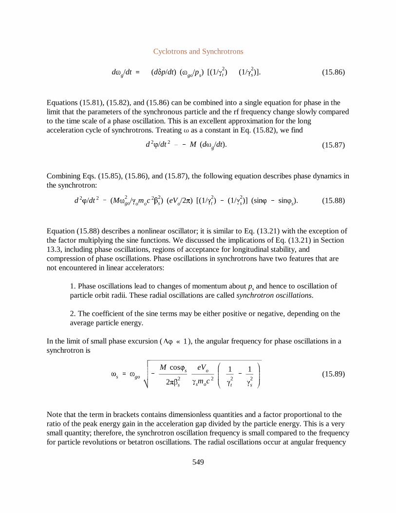
Cyclotrons and Synchrotrons
549
dωg/dt (dδp/dt) (ωgo/ps) [(1/γ2t ) (1/γ2
s)]. (15.86)
d 2φ/dt 2 M (dωg/dt). (15.87)
d 2φ/dt 2 (Mω
2go/γomoc
2β2s) (eVo/2π) [(1/γ2
t ) (1/γ2s)] (sinφ sinφs). (15.88)
ωs ωgo
M cosφs
2πβ2s
eVo
γsmoc2
1
γ2t
1
γ2s
(15.89)
Equations (15.81), (15.82), and (15.86) can be combined into a single equation for phase in thelimit that the parameters of the synchronous particle and the rf frequency change slowly comparedto the time scale of a phase oscillation. This is an excellent approximation for the longacceleration cycle of synchrotrons. Treatingω as a constant in Eq. (15.82), we find
Combining Eqs. (15.85), (15.86), and (15.87), the following equation describes phase dynamics inthe synchrotron:
Equation (15.88) describes a nonlinear oscillator; it is similar to Eq. (13.21) with the exception ofthe factor multiplying the sine functions. We discussed the implications of Eq. (13.21) in Section13.3, including phase oscillations, regions ofacceptance for longitudinal stability, andcompression of phase oscillations. Phase oscillations in synchrotrons have two features that arenot encountered in linear accelerators:
1. Phase oscillations lead to changes of momentum aboutps and hence to oscillation ofparticle orbit radii. These radial oscillations are calledsynchrotron oscillations.
2. The coefficient of the sine terms may be either positive or negative, depending on theaverage particle energy.
In the limit of small phase excursion ( ), the angular frequency for phase oscillations in a∆φ « 1synchrotron is
Note that the term in brackets contains dimensionless quantities and a factor proportional to theratio of the peak energy gain in the acceleration gap divided by the particle energy. This is a verysmall quantity; therefore, the synchrotron oscillation frequency is small compared to the frequencyfor particle revolutions or betatron oscillations. The radial oscillations occur at angular frequency
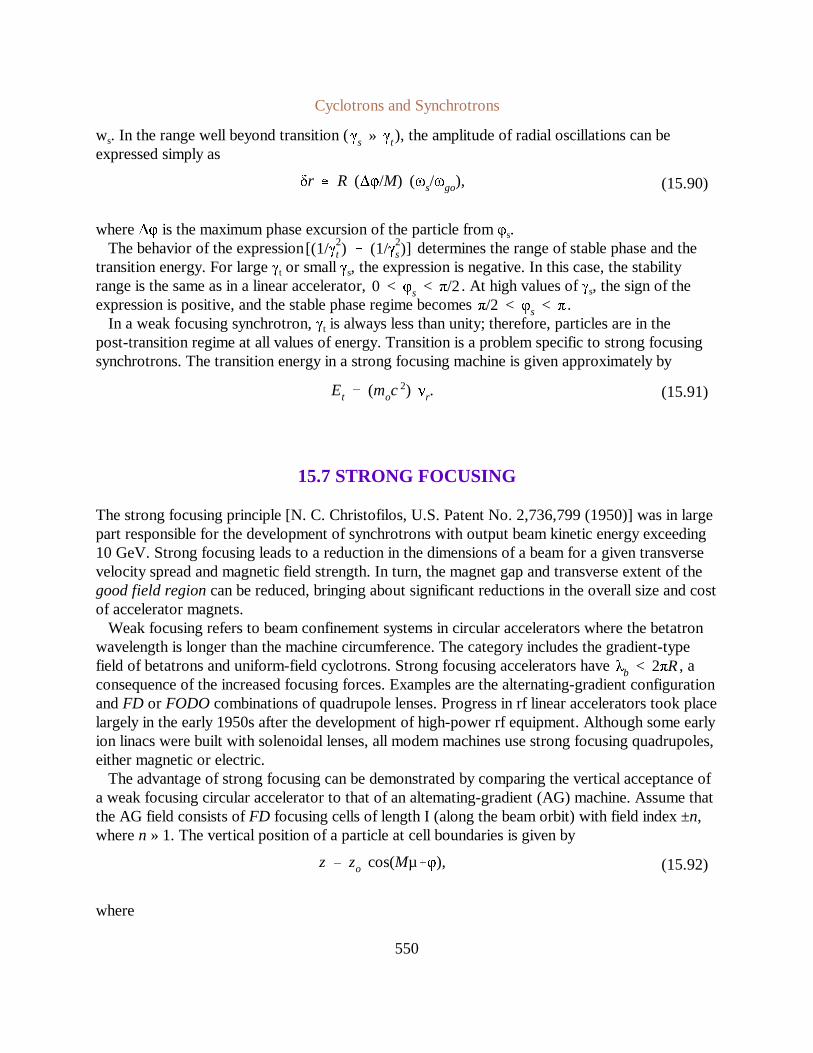
Cyclotrons and Synchrotrons
550
δr R (∆φ/M) (ωs/ωgo), (15.90)
Et (moc2) νr. (15.91)
z zo cos(Mµφ), (15.92)
ws. In the range well beyond transition ( ), the amplitude of radial oscillations can beγs » γtexpressed simply as
where∆φ is the maximum phase excursion of the particle fromφs.The behavior of the expression determines the range of stable phase and the[(1/γ2
t ) (1/γ2s)]
transition energy. For largeγt or smallγs, the expression is negative. In this case, the stabilityrange is the same as in a linear accelerator, . At high values ofγs, the sign of the0 < φs < π/2expression is positive, and the stable phase regime becomes .π/2 < φs < π
In a weak focusing synchrotron,γt is always less than unity; therefore, particles are in thepost-transition regime at all values of energy. Transition is a problem specific to strong focusingsynchrotrons. The transition energy in a strong focusing machine is given approximately by
15.7 STRONG FOCUSING
The strong focusing principle [N. C. Christofilos, U.S. Patent No. 2,736,799 (1950)] was in largepart responsible for the development of synchrotrons with output beam kinetic energy exceeding10 GeV. Strong focusing leads to a reduction in the dimensions of a beam for a given transversevelocity spread and magnetic field strength. In turn, the magnet gap and transverse extent of thegood field regioncan be reduced, bringing about significant reductions in the overall size and costof accelerator magnets.
Weak focusing refers to beam confinement systems in circular accelerators where the betatronwavelength is longer than the machine circumference. The category includes the gradient-typefield of betatrons and uniform-field cyclotrons. Strong focusing accelerators have , aλb < 2πRconsequence of the increased focusing forces. Examples are the alternating-gradient configurationandFD or FODO combinations of quadrupole lenses. Progress in rf linear accelerators took placelargely in the early 1950s after the development of high-power rf equipment. Although some earlyion linacs were built with solenoidal lenses, all modem machines use strong focusing quadrupoles,either magnetic or electric.
The advantage of strong focusing can be demonstrated by comparing the vertical acceptance ofa weak focusing circular accelerator to that of an altemating-gradient (AG) machine. Assume thatthe AG field consists ofFD focusing cells of length I (along the beam orbit) with field index ±n,wheren » 1. The vertical position of a particle at cell boundaries is given by
where

Cyclotrons and Synchrotrons
551
µ cos1 [cos( nωgo/vs) cosh( nωgo/vs)]
z zo cos(µS/l φ), (15.93)
z (zoµ/l) sin(µS/l φ). (15.94)
Av πzoz
o πz2o µ/l. (15.95)
z zo cos( nS/R φ). (15.96)
Av πz2o n/R. (15.97)
andM is the cell number. For , the orbit consists of a sinusoidal oscillation extending overµ 1many cells with small-scale oscillations in individual magnets. Neglecting the small oscillations,the orbit equation for particles on the beam envelope is
whereS, the distance along the orbit, is given byS= Ml. The angle of the orbit is approximately
Combining Eqs. (15.93) and (15.94), the vertical acceptance is
In a weak focusing system, vertical orbits are described by
Following the same development, the vertical acceptance is
In comparing Eqs. (15.95) and (15.97), note that the field index for weak focusing must be lessthan unity. In contrast, the individual field indices of magnets in the alternating gradient are madeas large as possible, consistent with practical magnet design. Typically, the field indices are chosento give . For the same field strength, the acceptance of the strong focusing system isµ 1therefore larger by a factor on the order ofR/l or N/2π, whereN is the number of focusing cells.The quantityN is a large number. For example,N = 60 in the AGS accelerator at BrookhavenNational Laboratory.
The major problem of strong focusing systems is that they are sensitive to alignment errors andother perturbations. The magnets of a strong focusing system must be located precisely. We shallestimate the effects of alignment error in a strong focusing system using the transport matrixformalism (Chapter 8). The derivation gives further insight into the origin of resonant instabilitiesintroduced in Section 7.2.
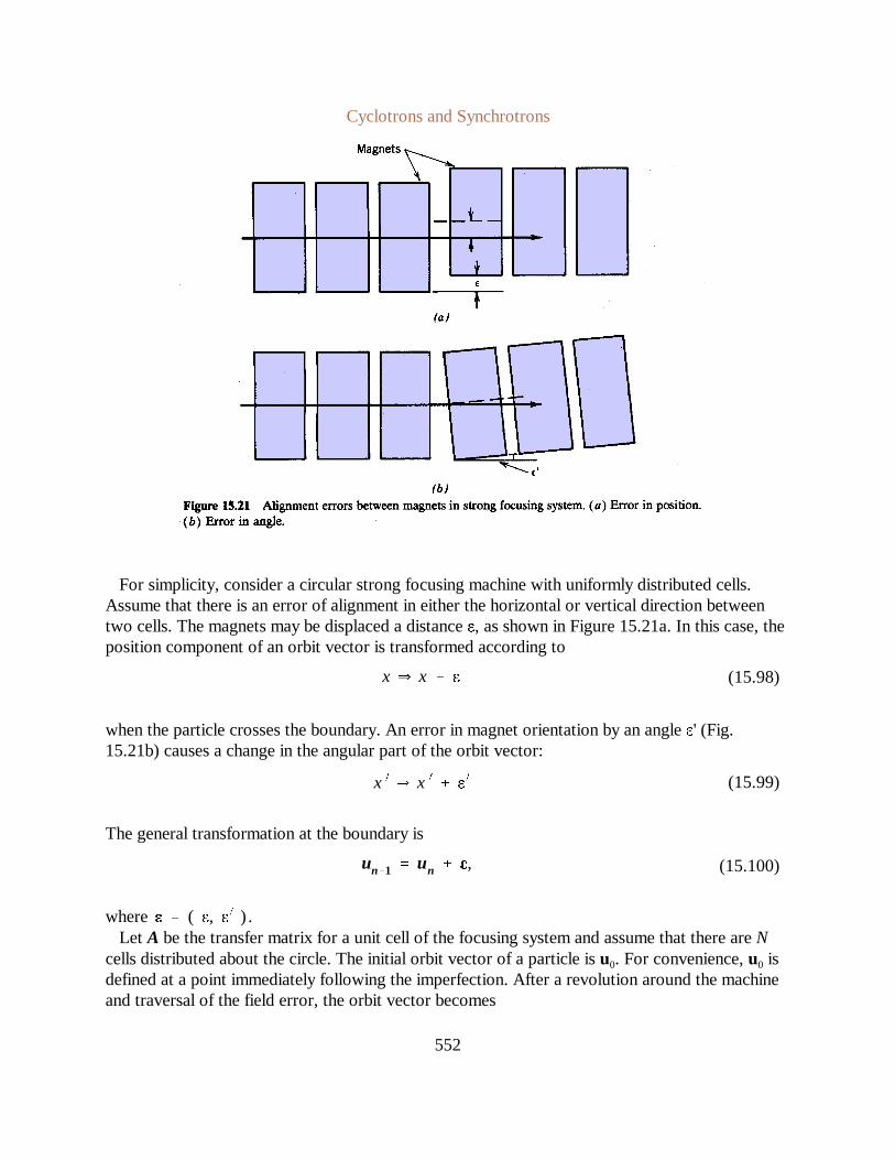
Cyclotrons and Synchrotrons
552
x x ε (15.98)
x x
ε (15.99)
un1 un ε, (15.100)
For simplicity, consider a circular strong focusing machine with uniformly distributed cells.Assume that there is an error of alignment in either the horizontal or vertical direction betweentwo cells. The magnets may be displaced a distanceε, as shown in Figure 15.21a. In this case, theposition component of an orbit vector is transformed according to
when the particle crosses the boundary. An error in magnet orientation by an angleε' (Fig.15.21b) causes a change in the angular part of the orbit vector:
The general transformation at the boundary is
where .ε ( ε, ε )
Let A be the transfer matrix for a unit cell of the focusing system and assume that there areNcells distributed about the circle. The initial orbit vector of a particle isu0. For convenience,u0 isdefined at a point immediately following the imperfection. After a revolution around the machineand traversal of the field error, the orbit vector becomes

Cyclotrons and Synchrotrons
553
uN A N u0 ε. (15.101)
u2N A N uN ε A 2N u0 (A N I ) ε, (15.102)
unN A nN u0 Dnε. (15.103)
Dn (A (n1)N A (n2)N
... A N I ). (15.104)
ε a1 ν1 a2 ν2. (15.105)
λ1 exp( jµ), λ2 exp(jµ). (15.106)
Dnε a1 ν1 exp[j(n1)Nµ] exp[j(n2)Nµ] ... 1
a2 ν2 exp[j(n1)Nµ] exp[j(n2)Nµ] ... 1 ,(15.107)
The orbit vector after two revolutions, is
whereI is the identity matrix. By induction, the transformation of the orbit matrix fornresolutions is
where
We found in Chapter 8 that the first term on the right-hand side of Eq. 1(15.103) corresponds tobounded betatron oscillations when stability criteria are satisfied. The amplitude of the term isindependent of the perturbation. Particle motion induced by the alignment error is described bythe second term. The expression forDn can be simplified using the eigenvectors (Section 8.6) ofthe matrixA: ν1 andν2. The eigenvectors form a complete set; any two-dimensional vector,includingε can be resolved into a sum of eigenvectors:
We found in Section 8.6 that the eigenvalues for a transfer matrixA are
where µ is the phase:advance in a cell. Substituting Eq. (15.106) in Eq. (15.103), we find
The sums of the geometric series can be rewritten as

Cyclotrons and Synchrotrons
554
Dnε
exp( jnNµ) 1exp( jNµ) 1
a1 ν1 aexp(jnNµ) 1exp(jNµ) 1
a2 ν2. (15.108)
Dnε [sin(nNµ/2)/sin(nµ/2)]
× [exp[ j(n1)Nµ/2)] a1 ν1 exp[j(n1)Nµ/2)] a2 ν2].(15.109)
µ 2πM/N, (15.110)
ν M. (15.111)
or, alternately,
The second term in braces is always bounded; it has a magnitude on the order ofε. The first termin brackets determines the cumulative effect of many transitions across the alignment error. Theterm becomes large when the denominator approaches zero; this condition occurs when
whereM is an integer. Equation (15.110) can be rewritten in terms ofν, the number of betatronwavelengths per revolution:
This is the condition for an orbital resonance. When there is a resonance, the effects of analignment error sum on successive revolutions. The amplitude of oscillatory motion grows withtime. The motion induced by an error when is an oscillation superimposed on betatronν Mand synchrotron oscillations. The amplitude of the motion can be easily estimated. For instance, inthe case of a position error of magnitudeε, it is .ε/sin(Nµ/2)

Cyclotrons and Synchrotrons
555
An alternate view of the nature of resonant instabilities, mode coupling, is useful for generaltreatments of particle instabilities. The viewpoint arises from conservation of energy and thesecond law of thermodynamics. The second law implies that there is equipartition of energybetween the various modes of oscillation of a physical system in equilibrium. In the treatment ofresonant instabilities in circularaccelerators, we included two modes of oscillation: (1) therevolution of particles at frequencyωgo and (2) betatron oscillations. There is considerablelongitudinal energy associated with particle revolution and, under normal circumstances, a smallamount of energy in betatron oscillations.In a linear analysis, there is no exchange of energy between the two modes. A field errorintroduces a nonlinear coupling term, represented by in Eq. (15.103). This term allowsDnε
energy exchange. The coupling is strong when the two modes are in resonance. The second lawimplies that the energy of the betatron oscillations increases. A complete nonlinear analysispredicts that the system ultimately approaches an equilibrium with a thermalized distribution ofparticle energy in the transverse and longitudinal directions. In an accelerator, the beam is lost onvacuum chamber walls well before this state is reached.
In a large circular accelerator, there are many elements of periodicity that can induce resonancecoupling of energy to betatron oscillations. In synchrotrons, where particles are contained for longperiods of time, all resonance conditions must be avoided. Resonances are categorized in terms offorbidden numbers of betatron wavelengths per revolution. The physical bases of some forbiddenvalues are listed in Table 15.5.

Bibliography
556
Bibliography
L. L. Alston (Ed.), High Voltage Technology, Oxford University Press, Oxford, 1968.
R. Bakish,Introduction to Electron Beam Technology, Wiley, New York, 1962.
A. P. Banford,The Transport of Charged Particle Beams, Spon, London, 1966.
A. H. W. Beck,Space Charge Waves and Slow Electromagnetic Waves, Pergamon Press,London, 1958.
M. Y. Bernard,Particles and Fields: Fundamental Equations, in A. Septier, Ed.,Focusing ofCharged Particles, Vol. 1, Academic, New York, 1967.
P.Bonjour, Numerical Methods for Computing Electrostatic and Magnetic Fields, in A. Septier,Ed.,Applied Charged Particle Optics, Part A, Academic, New York, 1980.
M. Born and E. Wolf,Principles of Optics, Pergamon Press, Oxford, 1965.
D.Boussard,Focusing in Linear Accelerators, in A. Septier, Ed.,Focusing of ChargedParticles, Vol. 2, Academic, New York, 1967.
H. Brechner,Superconducting Magnet Systems, Springer-Verlag, Berlin, 1973.
L. Brillouin, Wave Propagation in Periodic Structures, Dover, New York, 1953.
G. Brewer,Ion Propulsion - Technology and Applications, Gordon and Breach, New York,1970.
H. Bruck,Accelerateurs Circulaires de Particules, Presses Universitaires de France, Paris,1966.
R. A. Carrigen, F. P. Huson, and M. Month,Summer School on High Energy ParticleAccelerators, American Institute of Physics, New York, 1981.
J. D. Cobine,Gaseous Conductors, Dover, New York, 1958.
Bibliography
557
R. E. Collin,Foundations for Microwave Engineering, McGraw-Hill, New York, 1966.
T. Collins,Concepts in the Design of Circular Accelerators, in Physics of High EnergyParticle Accelerators(SLAC Summer School, 1982), American Institute of Physics, NewYork, 1983.
J.S. Colonias,Particle Accelerator Design - Computer Programs, Academic, New York,1974.
V.E. Coslett,Introduction to Electron Optics , Oxford University Press, Oxford, 1950.
P. Dahl,Introduction to Electron and Ion Optics , Academic, New York, 1973
H.A. Enge,Deflecting Magnets, in A. Septier, Ed.,Focusing of Charged Particles, Vol. 2,Academic, New York, 1967.
C.Fert and P. Durandeau,Magnetic Electron Lenses, in A. Septier, Ed.,Focusing of ChargedParticles, Vol. 1, Academic, New York, 1967.
J.F. Francis,High Voltage Pulse Techniques, Air Force Office of Scientific Research,AFOSR-74-2639-5, 1974.
J. C. Francken,Analogical Methods for Resolving Laplace's and Poisson's Equation, in A.Septier, Ed.,Focusing of Charged Particles, Vol. 1, Academic, New York, 1967.
A.Galejs and P. H. Rose,Optics of Electrostatic Accelerator Tubes, in A. Septier, Ed.,Focusingof Charged Particles, Vol. 2, Academic, New York, 1967.
C. Germain,Measurement of Magnetic Fields, in A. Septier, Ed.,Focusing of ChargedParticles, Vol. 1, Academic, New York, 1967.
G. N. Glasoe and J. V. Lebacqz,Pulse Generators, Dover, New York, 1965.
M. Goldsmith,Europe's Giant Accelerator, the Story of the CERN 400 GeV ProtonSynchrotron, Taylor and Francis, London, 1977.
H. Goldstein,Classical Mechanics, Addison-Wesley, Reading, Mass., 1950.
P. Grivet and A. Septier,Electron Optics, Pergamon Press, Oxford, 1972.
K. J. Hanszen and R. Lauer,Electrostatic Lenses, in A. Septier, Ed.,Focusing of ChargedParticles, Vol. 1, Academic, New'York, 1967.

Bibliography
558
E. Harting and F. H. Read,Electrostatic Lenses, Elsevier, Amsterdam, 1976.
W.V. Hassenzahl, R. B. Meuser, and C. Taylor,The Technology of Superconducting AcceleratorDipoles, in Physics of High Energy Particle Accelerators(SLAC Summer School, 1982),American Institute of Physics, New York, 1983.
P. W. Hawkes,Electron Optics and Electron Microscopy, Taylor and Francis, London, 1972.
P. W. Hawkes (Ed.),Magnetic Electron Lens Properties, Springer-Verlag, Berlin, 1980.
P.W. Hawkes, Methods ofComputing Optical Properties and Combating Aberrations forLow-Intensity Beams, in A. Septier, Ed.,Applied Charged Particle Optics, Part A, Academic,New York, 1980.
P. W. Hawkes,Quadrupoles in Electron Lens Design, Academic, New York, 1970.
P. W. Hawkes,Quadrupole Qptics, Springer-Verlag, Berlin, 1966.
R. Hutter,Beams with Space-charge, in A. Septier, Ed.,Focusing of Charged Particles, Vol. 2,Academic, New York, 1967.
J. D. Jackson,Classical Electrodynamics, Wiley, New York, 1975.
I. M. Kapchinskii, Dynamics in Linear Resonance Accelerators, Atomizdat, Moscow, 1966.
S. P. Kapitza and V. N. Melekhin,The Microtron , Harwood Academic, New York, 1978. (I. N.Sviatoslavsky (trans.))
E. Keil, Computer Programs in Accelerator Physics, in Physics of High Energy ParticleAccelerators(SLAC Summer -School, 1982), American Institute of Physics, New York, 1983.
O. Klemperer and M. E. Barnett,Electron Optics, Cambridge University Press, London, 1971.
A. A. Kolomensky and A. N. Lebedev,Theory of Cyclic Accelerators(trans. from Russian byM. Barbier), North-Holland, Amsterdam, 1966.
R. Kollath (Ed.),Particle Accelerators(trans. from 2nd German edition by W. Summer),Pittman and Sons, London, 1967.
P. M. Lapostolle and A. Septier (Eds.),Linear Accelerators, North Holland, Amsterdam, 1970.
L. J. Laslett,Strong Focusing in Circular Particle Accelerators, in A. Septier, Ed.,Focusing of

Bibliography
559
Charged Particles, Vol. 2., Academic, New York, 1967.
J. D. Lawson,The Physics of Charged-particle Beams, Clarendon Press, Oxford, 1977.
B. Lehnert,Dynamics of Charged Particles, North-Holland, Amsterdam, 1964.
A. J. Lichtenberg,Phase Space Dynamics of Particles, Wiley, New York, 1969.
R. Littauer,Beam Instrumentation, in Physics of High-energy Particle Accelerators(SLACSummer School, 1982), American Institute of Physics, New York, 1983.
J. J. Livingood,Principles of Cyclic Particle Accelerators, Van Nostrand, Princeton, NewJersey, 1961.
J. J. Livingood,The Optics of Dipole Magnets, Academic, New York, 1969.
M. S. Livingston (Ed.),The Development of High Energy Particle Accelerators, Dover, NewYork, 1966.
M. S. Livingston,High Energy Accelerators, Interscience, New York, 1954.
M. S. Livingston,Particle Accelerators, A Brief History , Harvard University Press,Cambridge. Mass., 1969.
M. S. Livingston and J. P. Blewett,Particle Accelerators, McGraw-Hill, New York, 1962.
G. A. Loew and R. Talman,Elementary Principles of Linear Accelerators, in Physics of HighEnergy Particle Accelerators(SLAC Summer School, 1982), American Institute of Physics,New York, 1983.
W. B. Mann,The Cyclotron, Methuen, London, 1953.
J. W. Mayer, L. Eriksson, and J. A. Davies,Ion Implantation in Semiconductors, Academic,New York, 1970.
N. W. McLachlan,Theory and Application of Matheiu Functions , Oxford University Press,Oxford, 1947.
A. H. Maleka,Electron-beam Welding - Principles and Practice, McGraw-Hill, New York,1971.
R. B. Miller, Intense Charged Particle Beams, Plenum Press, New York, 1982.

Bibliography
560
M. Month (Ed.),Physics of High Energy Particle Accelerators(SLAC Summer School,1982), American Institute of Physics, New York, 1983.
R. B. Neal (Ed.),The Stanford Two-mile Accelerator, Benjamin, Reading, Mass., 1968.
T. J. Northrup,The Adiabatic Motion of Charged Particles, Interscience, New York, 1963.
H. Patterson,Accelerator Health Physics, Academic, New York, 1973.
E. Perisco, E. Ferrari, and, S. E. Segre,Principles of Particle Accelerators, Benjamin, NewYork, 1968.
J. R. Pierce,Theory and Design of Electron Beams, Van Nostrand, Princeton, New Jersey1954.
D. Potter,Computational Physics, Wiley-Interscience, New York, 1973.
R. E. Rand,Recirculating Electron Accelerators, Harwood Academic, New York, 1984.
S. Ramo, J. R. Whinnery, and T. Van Duzer,Fields and Waves in CommunicationsElectronics, Wiley, New York, 1965.
E. Regenstreif,Focusing with Quadrupoles, Doublets and Triplets, in A. Septier, Ed.,Focusingof Charged Particles, Vol, 1, Academic, New York, 1967.
J. Rosenblatt,Particle Accelerators, Methuen, London, 1968.
W. Scharf,Particle Accelerators and Their Uses, Harwood Academic, New York. 1985.
S. Schiller, U. Heisig, and S. Panzer,Electron Beam Technology, Wiley, New York, 1982.
R.W. Southwell,Relaxation Methods in Theoretical Physics, Oxford University Press,Oxford, 1946.
A. Septier (Ed.),Applied Charged Particle Optics, Part A, Academic, New York, 1980.
A. Septier (Ed.),Applied Charged Particle Optics, Part B, Academic, New York, 1980,
A. Septier (Ed.),Applied Charged Particle Optics, Part C, Very-High Density Beams,Academic, New York, 1983.
A. Septier (Ed.).Focusing of Charged Particles, Academic, New York, 1967.

Bibliography
561
J. C. Slater,Microwave Electronics, Van Nostrand, Princeton, New Jersey, 1950.
K. G. Steffen,High Energv Beam Optics, Wiley-Interscience, New York, 1965.
E. Stuhlinger,Ion Propulsign for Space Flight, McGraw-Mll, New York, 1964.
P. Sturrock,Static and Dynamic Electron Optics, Cambridge University Press, London, 1955.
M. Tigner and H. Padamsee,Superconducting Microwave Cavities in Accelerators for ParticlePhysics, in Physics of High Energv Particle Accelerators(SLAC Summer School, 1982),American Institute of Physics, New York, 1983.
A. D. Vlasov,Theory of Linear Accelerators, Atomizdat, Moscow, 1965.
C. Weber,Numerical Solutions of Laplace's and Poisson's Equations and the Calculation ofElectron Trajectories and Electron Beams, in A. Septier, Ed.,Focusing of Charged Particles,Vol. 1, Academic, New York, 1967.
R. G. Wilson and G. R. Brewer,Ion Beans with Applications to Ion Implantation , Wiley,New York, 1973.
H. Wollnik, Electrostatic Prisms, in A. Septier, Ed.,Focusing of Charged Particles, Vol. 2,Academic, New York, 1967.
H. Wollnik, Mass Spectrographs and Isotope Separators, in A. Septier, Ed.,Applied ChargedParticle Optics, Part B, Academic, New York, 1980.
O. C. Zienkiewicz,The Finite Element Method in Engineering Science, McGraw-Hill, NewYork, 1971.
J.F. Ziegler,New Uses of Ion Accelerators, Plenum, New York, 1975.
V. K. Zworykin, G. A. Morton, E. G. Ramberg, J. Hillier, and A. W. Vance,Electron Opticsand the Electron Microscope, Wiley, New York, 1945.

Index
Index - 1
Index
Aberrations, lens, 132Acceleration column, electrostatic, 161, 227
breakdown in vacuum, 228fmaximizing breakdown voltage, 231
Acceleration gap, electrostatic focusing,121,125, 172Accelerator:
AGS (alternating gradient synchrotron),503
Alvarez, 456fAVF (azimuthally varying field)
cyclotron,501, 524fbetatron, 326fCockcroft-Walton, 210, 221coreless linear induction, 317fcoupled cavity, 459fcyclotron, 504fdrift tube linac (DTL), 456felectrostatic, 196fhigh energy, listing, 542linear, RF, 437felectron, 440fion, 452flinear induction, 283fpulsed power, 258fracetrack microtron, 493fradio-frequency quadrupole (RFQ), 482frecirculating linear induction, 328fseparated function synchrotron, 503,531fseparated sector;cyclotron, 501, 520fside-coupled linac, 465, 469spiral cyclotron, 502, 518fstrong-focusing synchrotron, 503superconducting. cyclotron, 502
synchrocyclotron, 502, 523fsynchrotron, 502, 531funiform-field cyclotron, 501, 504fVan de Graaff, 221fweak focusing synchrotron, 503, 534Wideroe, 453
Acceptance:of aperture, 140, 142of,focusing-system, 129, 140fof linear focusing system, 141flongitudinal, 420fof strong focusing system, 551of weak focusing system, 551
Alpha.particle, properties, 10Ampere, definition, 27Analog, electrostatic.@potential, 59fAngular, momentum, canonical, 126, 154
conservation, 126, 152fApparent accelerator length, 433fApplications, accelerator, 6Archimedean spiral, 519ATA accelerator:
cavity. geometry, 289, 290parameters, 288
Atomic mass number, A, 9Atomic number, Z, 9
Ballistic orbits, definition, 116Barium titanate, 85Beam, charged particle, 2
breakup instability,445fbunching, 423, 445confinement, 109cooling, 536

Index
Index - 2
current measurement, 276ffocus, 110generation process, 2flaminar, definition, 113matching, to focusing system, definition,
141position measurement, 278
Bessel equation, 369Bessel functions, 369fBeta-lambda linac, 456Beta-lambda/2 linac, 456Beta, relativistic factor, 18, 24Betatron, 326f
acceleration cycle, 333, 352fbetatron, condition, 333betatron oscillations,336, 342fcomparison to linear induction
accelerator,328fequivalent circuit, 348fextraction from, 345ffield biasing, 354fflux biasing, 354fgeometry, 328high current:
advantages, 327methods of achieving, 346f
injection into, 334f, 343finstantaneous circle, 334fmagnetic peeler, 345mapets, 348main orbit, 332maximum beam energy:
electrons, 330ions, 331f
orbit contraction coils, 345principle of operation, 327f
Betatron oscillations,138, 342constant energy, 145fradial and axial frequencies, 150reversible compressions, 336forbital stability, 150variable energy, 342
Betatron wavelength, 138in FD quadrupole channel, 193, 195
Bevatron, 547Bifrigence, 79Biot and Savart, law of, 28, 68Blumlein line, 250f
analysis of operation, 251circuit, 250fgeometry, 250properties, 253
Breakdown:spark:
condition for, in gas, 216electronegative gases, effect of, 218in gases, 213fin oil and water, 212Paschen's law, 217self-sustaining discharge, conditions, 216spark parameters, gases, 218
vacuum, 227fbreakdown levels, effect of pulselength,
229fbreakdown voltage, methods to increase,
230fconditioning of metal surfaces, effect, 229effect of beam, 231effect of exposed insulators, 229effect of surface whiskers, 227felectron multipactoring, 479fexposed insulators, breakdown levels,231factors affecting, 228fKilpatrick limit, RF voltage, 482with RF voltage, 478f
Brillouin diagram, 407Busch theorem, 152
Capacitance:coaxial capacitor, 200parallel plates, 199transmission line, 249
Capacitor, 199coaxial, 200f

Index
Index - 3
energy transfer between, 259fimpedance, 361parallel plate, 3 If, 85in pulsed power circuit, 233stored electrostatic energy density, 97fstored energy, 200
Cathode:cold, 229
effect of plasma closure, 229immersed, 156
Central orbit, 128Characteristic impedance:
coaxial transmission line, 241, 246Guillemin network,255f
LRC circuit, 235transmission line equivalent PFN, 254transmission lines, 241
Charge density, 33, 64Charge layer, 65Chromaticity, 168Clock, photon, 16, 19Cockcroft-Walton accelerator, 210f, 221Coercive force, 93Coherence, beam, 2Collider, 504, 540f
advantages, 541favailable reaction energy, 541lumiosity, 543particle dynamics in, 540
Complex conjugate, 359Complex exponential notation:
relation to trigonometric functions, 358theory, 357f
Confinement system, magnetic, 68Constancy, speed of light, 22Coordinates, cylindrical, 40fCoordinate transformations, 13fCorona discharge, 220Coulomb's law, 27Curl operator, 49fCartesian coordinates, 50Current, 27
Current density, 33, 60Current loop, magnetic fields of, 72fCurrent measurement, see Pulsed currentmeasurementCurrent sheet, 68Cutoff frequency, waveguide, 387, 390CVR (current viewing resistor), 276f
configurations, 277Cyclotron, 501
AVF:advantages, 527energy limits, 527nature of focusing forces, 526radial field variations, 524f
AVF focusing, 513f. See also Focusing byazimuthally varying fields
azimuthally varying field, 501beam extraction, 508dees, 506separated sector, 501
advantages, 527fspiral, 502superconducting, 502trim coils, 525funiform-field:
magnetic field, 506fmaximum beam energy, 51 Ifphase dynamics, 509fprinciples, 501, 504ftransverse focusing, 506f
Delta function, 33Demagnetization curve, 105Derivative:
first, finite difference form, 53second, finite difference form, 54
Deuteron, properties, 10Diamagnetism, 39Dielectric constant, relative, 79
plasma, 82water, 80
Dielectric materials, 64, 77faccelerator applications, 77

Index
Index - 4
properties, 78fsaturation, 79
Dielectric strength, 212Diode, 198
pulsed power, 258Dirichlet boundary condition, 56Dispersion, in waveguide, 387Dispersion relationship, 389Displacement current, 37, 39fDisplacement current density, expression, 39Displacement vector, D, 76, 80f
boundary conditions, 81, 83fDistribution, particle, 140
modification by acceleration gap, 427Divergence equation, 46Divergence operator, 47Divergence theorem, 47Domains, magnetic, 90Drift tube, 453Dynamics, particle, 8f
EAGLE, pulsed power generator, 259, 261Eddy current, 291Edge focusing, 132fEigenvalues, 184f
of 2X2 matrix, 185Eigenvectors, 184f
of 2X2 matrix, 185Elastic sheet, electrostatic potential analog,59Electric field, 29f, 45f
between parallel plates, 33boundary conditions on dielectric
material,81, 83fboundary conditions on metal surface, 51in charged cylinder, 64fenergy density, 97fminimization in electrostatic
accelerator,223fparaxial approximation, 111fproperties, 52
Electrodes, quadrupole field, 62
Electrolytic tank, electrostatic potentialanalog, 60fElectromagnetic oscillations, 40Electron, properties, 10Electron capture, 432Electron multiplication, in gases, 214f, 219Electron volt, eV, 9f, 23Electrostatic energy, storage, 85Elliptic integrals, 73f
series approximations, 74Equipotential surface., 52Energy:
kinetic:Newtonian, 12f, 23relativistic, 23
potential, 13relativistic, 22rest, 23
Envelope, beam, 110, 154Equipotential shields, 225fEulerian dfference method, 115Extractor, charged,particle, 121
Faraday rotation, 291fFaraday's law, 37, 38fFD focusing channel, 118f, 192fFerrite, 287, 293, 294, 299Ferromagnetic materials, 90f
accelerator applications, 77applications to magnetic circuits, 102boundary conditions, 95feddy currents, effects, 291fferrite, properties, 293f, 299hysteresis curve, 91fMetglas, properties, 293f, 299properties, 90frelative permeability, 90saturation, 90, 91saturation wave, 295silicon steel, properties,293f, 299skin depth, 291terminology, 93

Index
Index - 5
time-dependent,properties, 291fFFAG accelerator, 513Field biasing, betatron, 354fField description, advantages, 31Field emission, 227
enhancement by surface whiskers, 227fFowler-Nordheim equation, 227
Field equations, static, 46Field index, 148
expressions for, 148in isochronous cyclotron, 525
Field lines, 46approximation, 110ffocusing properties, 113fmagnetic:
relation to magnetic potential and vectorpotential, 71
relation to stream function, 72Finite difference calculations, 53
accuracy, 159fEulerian method, II 5, 15 9particle orbits, 157fparticle orbits in periodic focusing channel,
179ftime-centered method, 159two-step method, 159f
Flutter, AVF focusing, 514Flux, magnetic, 38, 102Flux biasing, betatron, 354fFlux forcing, 305f, 350Flux function, 153
relation to vector potential and streamfunction, 154FNAL accelerator (Tevatron), 536ff-number, 117Focal length, 116
relation to transfer matrix, 173systems with curved axes, 130
Focusing, radial, in uniform magnetic field,146Focuging by azimuthally varying fields, 513f
in AVF cyclotron, 526
flutter, 514flutter amplitude, 514flutter function, 514hills and valleys, definition, 514modulation function, 514nu, vertical and horizontal, 517fparticle orbits, 514fsector, definition, 514separated sector magnets, 521fseparated sector magnets with spiral
boundaries, 521spiral pole boundaries, effect, 518Thomas focusing, 514ftransfer matrices, 517f
Focusing cell, defintion, 179Focusing channels, periodic, 165f
FODO, 533quadrupole, stability condition,188, 192fquadrupoles, 187f, 550fstability properties,183f
Focusing force, average in a periodic system,139Focusing lattice, 532Foil focusing, 124Force, 11, 22
centrifugal, 41between charges, 27Coriolis, 42electric, 26f, 30magnetic, 26f, 30fvirtual, 41
Fowler-Nordheim equation, 227Frames of reference, 13Frequency domain, 198, 240Fringing flux, 102
Gamma, relativistic factor, 18Gap, vacuum, effect in magnetic circuit, 100Gaussian optics, 108Gradient, definition, 13Grading, voltage, 223fGrading rings:

Index
Index - 6
effect on vacuum insulation, 227f, 230,231,232
electrostatic focusing by, 161electrostatic potential variations, 163f
Grid focusing, 124Group velocity, 387, 449
in coupled cavities, 466Guillemin network,255f
choice of circuit elements, 257properties, 257
Gyrocenter, 44Gyrofrequency, 44Gyroradius, 44
in cyclotron, 506
Hamiltonian dynamics, 154Harmonic oscillator, damped, solution,359fHelmholtz coils, 75Hysteresis, 93Hysteresis curve:
examples, 94ferromagnetic materials, 91fmeasurement, 91saturation, 92f
Image:charged particle, 110definition, 117formation, equations, 119, 175fintensifier, 110
Image plane, 117Image space, 116Impedance, 360
capacitor, 361combinations, 362inductor, 361resistor, 360transformation on transmission line, 383
Inductance:coaxial inductor, 201solenoid inductor, 202transmission line, 249
Induction, magnetic, 37, 39Inductive isolation, 283Inductive switching, 263f
advantages, 263circuit analysis, 263fcircuit design, 264, 266constraints, power compression, 264ffor high power transmission line, 266power compression, 264fpulse shaping, 267
Inductor, 199coaxial, 201in energy storage circuit, 236impedance, 361solenoid, 202stored energy, 200
Inertial frame, 15Instability:
orbital, 150in FD quadrupole channel, 188f, 192fin separated sector magnets, 521fin strong focusing system, 554in thin lens array, 182f
resonance, 143fin circular accelerator with FD focusing,
195conditions for, 145
models for, 144Insulation, 211f
vacuum, 227foptimization, 229
Insulator:gas, properties, 213high voltage vacuum, 85fproperties of some solids and liquids, 212pulsed behavior, 212self-healing, 213transformer oil, properties, fast pulse, 212water, properties, fast pulse, 212
Integrator, passive, 203fInvariance, coordinate transformation, 15Ion, properties, 9

Index
Index - 7
Irises, in slow wave structures, 394Iris-loaded waveguide, see slow wavestructureISR (Intersecting Storage Ring), 539
KEK 2.5 GeV accelerator, 442fKerr effect, 281Kilpatrick limit, 482Klystron, 376
Ladder network, 210fadvantages, 211circuit, 210
LAMF accelerator, 465, 468Laminar beam, 113, 140, 155Laplace equation, 50f
analog solutions, 58fcylindrical coordinates, 57with dielectrics, 81finite difference formulation, 53fcylindrical coordinates, 58numerical solution with dielectrics, 81numerical solutions, 53f
Laplacian operator, 50Laser, electron-beam-controlled discharge,21Law, relativistic velocity addition, 22Laws of motion:
Cartesian coordinates, 12cylindrical coordinates, 40Newton's first, 11Newton's second, 11
LC generator, 238fLeakage current, 285
in ferrite core induction accelerator, 294fin laminated core, 298measurement, 298f
Leakage flux, 102Length, apparent, 20Lens, charged particle, 108f
determination of properties, 119einzel, 124
electrostatic, unipotential, 119, 124electrostatic aperture:
focal length, 121properties, 119f
electrostatic immersion, 58,121felectric fields, 122focal length, 124particle orbits, 123, 164potential variation, 164transfer matrix, 172f
electrostatic quadrupole, 136facet, 60inclined sector magnet boundary, 132fmagnetic quadrupole, 134f
doublet and triplet, 176ffocal lengths, 135particle orbits, 135
magnetic sector, 127fpower, 117properties, 115fsolenoidal magnetic, 125f
focal length, 127particle orbits, 126f
thick, definition, 116thin:
definition, 115, 116transfer matrix, 168
toroidal field sector, 13ifLinear accelerator:
induction, 283faccelerating gradient:
comparison with and withoutferromagnetic cores, 323f
expressions, 315ffactors affecting, 316f
ATA accelerator, 288fcavity:
equivalent circuit, 286principles of operation, 284, 286
comparison with betatron, 283, 328fcompensation circuits, 31 Ifcoreless:

Index
Index - 8
limitations, 323principles of operation, 319f
coreless geometries, 317core reset, 307fcore saturation, problems, 304damping resistor, role of, 307electric field distribution in cavity, 313fferrite core cavity, 294fflux forcing, 305injector configuration, 302laminated cores, 297leakage current, 285, 295, 298longitudinal beam confinement:
electrons, 435fions, 427f
longitudinal core stacking, 302longitudinal dynamics, 426fradial core stacking, 302f, 306frecirculating, 328frelationship to electrostatic accelerator,
284freset circuit:
ferrite core cavity driven by Blumleinline, 309f
long pulse accelerator, 308properties, 307
series configuration, 286, 287volt-second product, 287
RF:choice of waveguide, 406fenergy spread, 426individually phased cavities, particle
dynamics, 411findividually phased cavity array, 398, 456injection into, 423Kilpatrick limit, 482micropulsewidth, 425multipactoring, 479radio-frequency quadrupole (RFQ), 482frepresentation of accelerating field, 416resolution of electric fields into travelling
waves, 414f
shunt impedance, definition, 452vacuum breakdown in, 478f
Linear accelerators, advantages, 437Linear electron accelerator, RF, 440f
beam breakup instability,445f, 447energy flow, 449ffrequency equation, 447fgeometry, 440f, 451finjection into, 445optimizing for maximum beam energy,450fproperties, 440fpulse shortening, 445fradial defocusing by RF fields, 478regenerative beam breakup instability, 446transverse instability,445f
Linear focusing force, properties, 138Linear ion accelerator, 452f
Alvarez linac. 456fbeta-lambda structure, 456beta-lambda/2 structure, 456comparison with electron accelerator, 452coupled cavity, 459fdisk and washer structure, 466, 473drift tube linac, 456f
features, 459gap coefficient, 475post-couplers in DTL, 459radial defocusing by RF fields, 476resonant cavities in, 455side-coupled linac, 465, 469transit-time factor, 473fWideroe configuration, 453f
Linear optics, 108Lorentz contraction, 18fLorentz force law, 3, 31LRC circuit:
equations, 233fpower loss, resonant circuit, 363fQ parameter, 364fresonance, 362fresonance width, 363, 365solutions:

Index
Index - 9
critically damped, 235overdamped, 235underdamped, 235
L/R time, 204Luminosity, 543
Magnetic circuits, 99fpermanent, 103f
Magnetic core:betatrons, 348fconstruction, 291electric field distribution, 299fenergy losses, 99ferrite, properties, 287flux forcing, 305fin inductive accelerator, 287in inductive switches, 263flaminated core construction, 297laminated cores, time-dependent properties,
297fin magnetic circuit, 101reset, 264, 307fsaturation, problems, 303fsaturation wave, 295
Magnetic field, 30f, 45f, 93boundary conditions, ferromagnetic
materials, 95fof current loop, 74felectro-optic measurements, 281fenergy density, 97f
calculated from hysteresis curve, 98fexamples, 67fwith gradient, properties, 148of Helmholtz coils, 75near current-carrying wire, 67near two current carrying wires, 71paraxial approximation, 112fsector, 127fsector with gradient, transfer matrix, 170solenoid, 68fin torus, 68f
Magnetic intensity, H, 76, 88f, 93
Magnetic materials, 87fhard, definition, 93properties, 87fsoft, definition, 93
Magnetic mirror, 112f, 147fproperties of field in, 148f
Magnetic moment, 87fclassical value, 87quantum mechanical value, 88
Magnetic poles, 95fdetermination of shape, 148North-South convention, 96saturation effects, 96
Magnetization curve, virgin, 92Magnetomotive force, 102Magnets:
AGS (alternating gradient synchrotron), 53betatron, 348fcyclotron, 506, 514dipole, 532fquadrupole, 532fsextupole, 532fsynchrotron, 532f
superconducting, 537Magnification, by lens, 118MAMI accelerator, 494, 496Marx generator, 237fMass, 10f
relativistic, 22Mathieu equations, 484Matrix, transfer, 165f
of AVF system, 517fof AVF system with spiral boundaries, 518of circular accelerator with alignment error,
552fcombining optical elements, 173fdeterminant, 172of drift space, 169eigenvectors and eigenvalues, 184fof immersion lens, 172inverse, 171fmultiplication, rules of, 174

Index
Index - 10
operations, 167orbital stability condition, 186properties of, 167f, 172of quadrupole channel, 188, 192of quadrupole doublet, 177fof quadrupole lens, 166fof quadrupole triplet, 179raising to power, 183frelation to phase advance, 186relation to principal planes and focal lengths
of lens, 173of sector magnet with gradient, 170fof thin lens, 168trace, 184
Maxwell equations, 33felectromagnetic form, vacuum, 368listing, 34static form, 46
Mean free path, for collisions, 214Mechanics, Newtonian, 10fMesh, finite difference, 53, 55Microbursts, 229Mcrotron, see Racetrack microtronModulator, pulsed power, see Pulsed powergeneratorMomentum:
Newtonian, 11relativistic, 22
Multipactoring, 479f
Necktie diagram, 192, 194Negative lens effect, 121Neptune C, pulsed power generator, 259,260Neumann boundary condition, 56, 58Nu, 142f
for AVF cyclotron, 527for AVF focusing system, 517ffor AVF focusing system with spiral
boundaries, 519definition, 143forbidden values, 533, 554f
for separated sector magnets with spiralboundaries, 521Nwnerical solutions:
first order differential equation, 158fLaplace equation, 53fparticle orbits, 157fparticle orbits in acceleration column, 161particle orbits in immersion lens, 164second order differential equation, 157f
Object plane, 117Object space, 116Oil, transformer:
in coaxial transmission line, 250insulation properties, 212
Orange spectrometer, 131Orbit, particle:
in AVF focusing system, 514fconstant magnetic field, 43f, 146numerical solutions, 157fin quadrupole channel, 189freversible compression, 337fin RF quadrupole field, 484fin separated sector cyclotron, 529in thin lens array, 181f
Orthogonality, of eigenvectors, 184
Paramagnetic materials, 88, 90Paraxial approximation, basis, 110Paraxial ray equation, 151, 154f
complete relativistic form, 156non-relativistic forms, 157validity conditions, 155
Particle, properties, 9fPaschen law, 217fPeaking capacitor circuit, 259fPeriodic focusing, 165f
choice of phase advance, 191orbit solutions, 179fstability condition, 186stability properties,183f
Permanence, magnetic, 102

Index
Index - 11
Permanent mapets, 103fenergy product, 106examples of calculations, 107load line, 107material properties, 104operating point, 105fpermanence coefficient, 107
Permeability, relative, 88fsmall signal value, 91
Phase, particle, definition, 410f, 414Phase advance:.
choice of optimum, 191definition, 181relation to transfer matrix, 186
Phase dynamics, 408fasymptotic-phase, electron accelerator, 445compression of phase oscillations, 424effective longitudinal force, 419electron capture, 432, 445limits of phase oscillations, 419linear, accelerator, electrons, 430flinear induction accelerator:
electrons, 435fions, 426f
longitudinal acceptance, 420flongitudinal potential diagram, 420fin racetrack microtron, 498frelation between kinetic energy error and
phase, 424relativistic particles, 430fin synchrotron, 544ftrapping particles in RF buckets, 422in uniform-field cyclotron, 509
Phase equations, 414fapplications, 408approximation:
slowly varying vs, 418, 419small amplitude, 418
small amplitude, 424fgeneral form, 417relativistic limit, 430, 432for synchrotron, 549
for uniform-field cyclotron, 511Phase oscillation frequency, 418Phase space, 140
conservation of phase area, 339, 341orbits, reversible compression, 339relativistic particles, 343
Phase stability,410fcondition:
linear accelerator, 413synchrotron, 550
PIGMI accelerator, 467Pion, 18Planck constant, 88Plasma, dielectric constant, 82Plasma closure, cold cathode, 229Plasma source, inductively coupled, 38, 39Pockels effect, 281Poisson equation, 65f
numerical solution, 66fPolar molecules, 77fPotential:
absolute, 36, 155electrostatic, 34f, 50
in charge cylinder, 66definition, 36expressions, 36, 37
magnetic, 53, 70fanalogy with electrostatics for
ferromagnetic poles, 95relation to field lines, 71vector, 34f, 70f
analogy with field lines, 70of current loop, 72fdefinition, 37expressions, 37relation to flux function, 154of two current-carrying wires, 71
Power compression, 259frole of peaking capacitor circuit, 260f
Power supplies, high voltage, 204fcircuit, half-wave rectifier, 209ladder network, 210f

Index
Index - 12
ripple, 209Precession, orbit, 150Primary, transformer, 204
inductance, 205Principal plane, 116
relation to transfer matrix, 173in system with curved axes, 130
Proton, properties, 10Pulsed current measurement:
current viewing resistor (CVR), 276felectro-optical, 281fmagnetic pickup loops, 278fRogowski loop, 279f
Pulsed power generator, 231faccelerator applications, 232Blumlein line, 250fcharacteristic impedance, 235critically damped LRC circuit, properties,
235diagnostics on, 267fimpulse generators, 236finductive energy storage, 236LC generator:
circuit, 238fproperties, 239f
Marx generator:circuit, 237properties, 238
matching condition to load, 235peaking capacitor circuit, 260power compression cycle, 258fproperties, 231pulse-forming-network, 254fpulse shaping by saturable core inductors,
267risetime of current and power, 204role of saturable core inductor switches,
263series transmission line circuits, 250fsimple model, 202switching by saturable core inductors, 266transmission line:
circuit, 248properties, 241f
Pulsed voltage measurement, 270fbalanced divider, 273capacitive divider, 273
compensated, 276capacitive pickup, 275fcompensated divider with water resistor,
273finductive correction with magnetic pickup
loop, 278finductive divider, 273limitations,267fresistive divider:
compensation, 272fsources of error, 271f
Pulse-forming-network, 254fcharacteristic impedance, 254Guillemin network,255ftransmission line equivalent circuit, 254
Q parameter:combinations, 379cylindrical cavity, 373definition, 364resonant circuit, 365
Quadrupole field:electrostatic, 61felectrostatic potential, 62magnetic, 96
Quadrupole focusing channel, 187betatron wavelength, 193, 195choice of phase advance, 191resonance instabilities in circular
accelerator, 194fstability condition,188, 192f
Quadrupole lens:doublet, 176f
transfer matrix, 177approximate form, 178
magnetic, 134radio-frequency (RF), 483f

Index
Index - 13
transfer matrix, 166approximate form, 178
triplet, 178transfer matrix, 179
Racetrack microtron, 493fadvantages 493double-sided microtron (DSM), 498finjection into, 494fgeometry, 493fproblems of focusing and beam breakup
instability, 497fspatial separation between orbits, 497synchronous particle condition, 495f
Radio-frequency quadrupole accelerator(RFQ), 482f
dipole mode, 493electric fields in, 487electrode design, 490felectromagnetic modes in, 492felectrostatic approximation, 483electrostatic potential, expression for, 490geometry, 486, 491, 492ion injection application, 482flimit on accelerating gradient, 490manifold, 493motion of synchronous particle, 487ftransverse focusing in, 483f, 489f
RC time, 203Rectifier, half-wave, 209Relativity, special, 15f
postulates of, 15fRemanence flux, 93
magnetic, 102Residuals, method of successiveoverrelaxation, 55Resistivity, volume, 60Resistor, 198f
impedance, 360power dissipation, 199
Resonance, 363Resonant accelerators, properties, 356
Resonant cavity, 362analogy with quarter wave line, 384arrays for particle acceleration, 455fcomparison with induction linear
accelerator cavity, 367coupled array, 459fcylindrical, 367f, 371fdisk and washer structure, 466, 473electric and magnetic coupling between
cavities, 460high order modes, effect, 373finductive isolation in, 362flumped circuit analogy, 362fmatching power input, 380, 385for particle acceleration, 455power exchange, 376, 385power losses, 363f, 373Q parameter, 373re-entrant, 365fresonance width, 365, 373resonant modes, 367f, 371frole in RF accelerators, 454side coupled cavities, 469stored energy, 373transformer properties, 377
Resonant circuits, 362fResonant modes, 367f
of array of coupled cavities, 462fdegeneracy, 376nomenclature, 371pi mode, coupled cavities, 464pi/2 mode, coupled cavities, 466fof seven coupled cavities, 464TE vs. TM, 391TE11, 393TE111, 374fTEM, 387f, 399fTE210, in RFQ, 493TM10, 388, 390fTMn0, dispersion relationship, 400TM010, cylindrical cavity, 370f, 372, 373TM010, in beta-lambda and beta-lambda/2

Index
Index - 14
structures, 456TM020, cylindrical cavity, 370, 372TM0n0, cylindrical cavity, 370, 371TM110, 445fof two coupled cavities, 460f
Rest energy, 9Rest frame, 13Rest mass, 11Reversible compression, particle orbits:
of phase oscillations,424fproperties, 338frelativistic, 343
RF bucket, 422Rogowski loop, 279f
geometry, 280properties, 281sensitivity, 280, 281theory, 279f
Rogowski profile, 219f
Saturation induction, 93Saturation wave, in magnetic core, 295fSecondary, transformer, 204Secondary emission coefficient, 215, 479Sector magnet, 127f
focal properties, 45 degrees, 498fhorizontal direction, definition, 128with inclined boundaries, focusing, 520fvertical direction definition, 128
Septum, for beam extraction, 508Shunt impedance, 452Side coupled linac, 465, 469fSIN cyclotron, 528fSkin depth, 291, 293, 373Slow wave, non-existence in uniformwaveguides, 393Slow wave properties:
non-existence in uniform waveguide, 393radial defocusing of captured particles, 476frest-frame description:
non-relativistic, 475frelativistic, 477
Slow wave structures, 393fcapacitively loaded transmission line, 394f,
401 fdispersion relationship, iris-loaded
waveguide, 403fenergy flow in, 449individually phased cavity array, 398iris-loaded waveguide, 395f
dispersion relationship, 403ffrequency equation, 447f
Solenoid, 68Solenoidal magnetic lens, 125fSpace charge, 64Sparks, 216Spectrograph, 180 degree for chargedparticles, 128Spectrometer:
dual-focusing magnetic, 133forange, 131
Speed of light, c, 15Squares, method of, 53SSC (Superconducting Super Collider), 543Stability bands, 189Stanford Linear Accelerator (SLAC), 442Stationary frame, 13Stoke's theorem, 48fStorage ring, 503f, 539Stream function, 72Strong focusing, 550f
acceptance, 551comparison with weak focusing, 550feffect of alignment errors
Successive overrelaxation, method of, 55fwith space charge, 67
SUPERFISH code, 455Superposition, electric and magnetic fields,64, 89Surface charge, dielectric materials, 79Surface current, paramagnetic andferromagnetic materials, 88Switch, 198
closing, 198, 231

Index
Index - 15
opening, 198, 236saturable core inductor, 263fspark gap, high power, 259
Synchrocyclotron, 502, 523fbeam extraction from, 523fcomparison with cyclotron, 523
Synchronous particle, 410fcondition for:
individually phased cavities, 411fracetrack microtron, 495fWideroe accelerator, 454
Synchronous phase, 411Synchrotron, 502, 531f
energy limits, 535focusing cell, definition, 533geometry, 531flongitudinal dynamics, 544fmagnets, separated function, 532principles of operation, 531fstrong focusing in, 550fsuperperiod, 533synchronization condition, 546fsynchrotron radiation in electron
accelerator, 535ftransition energy, 544, 549ftypes of, 502fweak focusing, 534
Synchrotron oscillations,544, 549Synchrotron radiation, 535
beam cooling by, 536energy limits, electron synchrotron,535fexpression for, 535
Tandem Van de Graaf accelerator, 222, 224Telegraphist's equation, 245Termination, of transmission line, 246f, 381fThick lens equation, 119Thin lens array:
orbital stability,182, 187particle orbits in, 179f, 187
Thin lens equation, 119Time dilation, 16f
Time domain, 198, 240Topics, organization, 4fToroidal field sector lens, 131Torus, 68fTownsend coefficient, first, 214, 216Townsend discharge, 220Transformation:
Galilean, 13fLorentz, 20fNewtonian:
kinetic energy, 14velocity, 14
relativistic, velocity, 21Transformer, 204f
air-core, 204fdroop, 207fenergy losses, 208equations, 206equivalent circuit models, 206fimpedance transformation, 207pulse, 207role of ferromagnetic material, 207fvolt-second product, 209
Transform function, of a diagnostic, 272Transit-time factor, 473fTransmission line, 240f
capacitance of, 249capacitively loaded, 343fdispersion relationship, 401fcoaxial, properties, 240fconditions for TEM wave, 243current diagnostics in high power line, 277equations, time domain, 243ffrequency domain analysis, 380fat high frequency, 388inductance of, 247lumped element circuit model, basis, 242fmatched termination, 247parallel plate, properties, 241as pulsed power modulator, 246fpulse-forming-network equivalent, 254fpulselength, as pulsed power modulator,

Index
Index - 16
249quarter-wave line, 384radial, properties, 317freflection coefficient, 382relation to pulse forming networks, 240solutions of wave equation, properties,
245fstripline, properties, 241termination, 246transformer properties, 382ftransmission coefficient, 382two-wire, properties, 241velocity of wave propagation, 246voltage diagnostics in high power line, 275fwave equation, 245wave reflection at termination, 246f, 381f
Trimming coils, in cyclotron, 526Triton, properties, 10Two-terminal elements, 197f
UNILAC accelerator, 471
Van de Graaff accelerator, 221equipotential shields in, 225fminimizing electric field stress,223fparameters, 221fprinciple of operation, 221ftandem, 222, 224voltage grading, 223fvoltage measurements, 269f
Vector, particle orbit, 166, 183fVelocity, 11Voltage, measurement, 267f
generating voltmeter, 269fresistive divider, 269resistive shunt, 268fsee also Pulsed voltage measurement
Water:in coaxial transmission line, 250dielectric properties, 80
microwave absorption, 80
electrostatic energy storage, 85, 212insulation properties, fast pulse, 212in radial transmission line, 319resistors, 271
Waveguides, 386fapplications, 387comparison to transmission line, 387cutoff frequency, 387, 392dispersion in, 387lumped-circuit-element analogy, 387fphase velocity in, 393properties, 387fslow waves, see Slow wave structuressolutions for TM10 mode, 391f
Weak focusing, 150Whiskers, 227f
effect on vacuum insulation, 229fenhancement of field emission on metal
surface, 227removal by conditioning, 229vaporization,,227f
Wideroe accelerator, 453flimitations, 454synchronous particle in, 454
Work, definition, 12
ZGS (Zero-gradient Synchrotron), 133, 534