Radu Tr^ mbit˘a˘s Purpose Simulation Output Analysis for a ...math.ubbcluj.ro/~tradu/OutputDataAnal.pdf · Output Analysis for a Single Model Radu Tr^ mbit˘a˘s Purpose Types of

Output Analysisfor a Single Model

Radu Trımbitas

Purpose

Types ofSimulation

Stochastic Natureof Output Data

Measures ofPerformance

Point estimator

Confidence-IntervalEstimation

Output Analysisfor TerminatingSimulations

Statistical BKG

CIs with SpecifiedPrecision

Quantiles

EstimatingProbabilities andQuantiles fromSummary Data

Output Analysisfor Steady-stateSimulations

Initialization Bias

Error Estimation

References

Output Analysis for a Single ModelOutput Analysis

Radu Trımbitas

Faculty of Math and CS - UBB

1st Semester 2010-2011


Radu Trımbitas

Purpose

Types ofSimulation



Point estimator



Statistical BKG


Quantiles



Initialization Bias

Error Estimation

References

Purpose

I Objective: Estimate system performance via simulation

I If θ is the system performance, the precision of theestimator θ can be measured by:

I The standard error of θI The width of a confidence interval (CI) for θ.

I Purpose of statistical analysis:

I To estimate the standard error or confidence interval.I To figure out the number of observations required to

achieve a desired error or confidence interval.

I Potential issues to overcome:

I Autocorrelation, e.g. inventory cost for subsequentweeks lack statistical independence.

I Initial conditions, e.g. inventory on hand and number ofbackorders at time 0 would most likely influence theperformance of week 1.


Radu Trımbitas

Purpose

Types ofSimulation



Point estimator



Statistical BKG


Quantiles



Initialization Bias

Error Estimation

References

Types of Simulation

I Distinguish the two types of simulation:

I transient vs.I steady state - a simulation whose objective is to study

long-run or steady-state behavior of nonterminatingsystem

I Illustrate the inherent variability in a stochasticdiscrete-event simulation.

I Cover the statistical estimation of performancemeasures.

I Discusses the analysis of transient simulations.

I Discusses the analysis of steady-state simulations.


Radu Trımbitas

Purpose

Types ofSimulation



Point estimator



Statistical BKG


Quantiles



Initialization Bias

Error Estimation

References

Types of Simulation I

I A distinction is made between terminating (or transient)versus non-terminating simulations

I Terminating simulation:

I Runs for some duration of time TE , where E is aspecified event or set of events that stops thesimulation.

I Starts at time 0 under well-specified initial conditions.I Ends at the stopping time TE .I Bank example:

I Opens at 8:30 am (time 0) with no customers presentand 8 of the 11 teller working (initial conditions)

I closes at 4:30 pmI Time TE = 480 minutes.

I The simulation analyst chooses to consider it aterminating system because the object of interest is oneday’s operation.

I TE may be known from the beginning or it may not


Radu Trımbitas

Purpose

Types ofSimulation



Point estimator



Statistical BKG


Quantiles



Initialization Bias

Error Estimation

References

Types of Simulation II

I Non-terminating simulation:

I Runs continuously, or at least over a very long period oftime.

I Examples: assembly lines that shut down infrequently,hospital emergency rooms, telephone systems, networkof routers, Internet.

I Initial conditions defined by the analyst.I Runs for some analyst-specified period of time TE .I Study the steady-state (long-run) properties of the

system, properties that are not influenced by the initialconditions of the model.

I Whether a simulation is considered to be terminating ornonterminating depends on both

I The objectives of the simulation study andI The nature of the system


Radu Trımbitas

Purpose

Types ofSimulation



Point estimator



Statistical BKG


Quantiles



Initialization Bias

Error Estimation

References

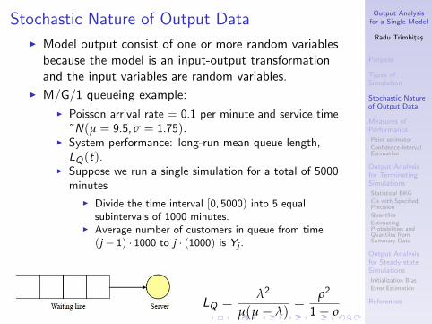
Stochastic Nature of Output Data

I Model output consist of one or more random variablesbecause the model is an input-output transformationand the input variables are random variables.

I M/G/1 queueing example:

I Poisson arrival rate = 0.1 per minute and service time˜N(µ = 9.5, σ = 1.75).

I System performance: long-run mean queue length,LQ(t).

I Suppose we run a single simulation for a total of 5000minutes

I Divide the time interval [0, 5000) into 5 equalsubintervals of 1000 minutes.

I Average number of customers in queue from time(j − 1) · 1000 to j · (1000) is Yj .

LQ =λ2

µ(µ− λ)=

ρ2

1− ρ


Radu Trımbitas

Purpose

Types ofSimulation



Point estimator



Statistical BKG


Quantiles



Initialization Bias

Error Estimation

References

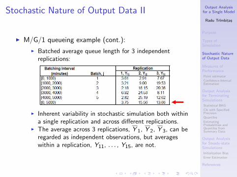
Stochastic Nature of Output Data II

I M/G/1 queueing example (cont.):

I Batched average queue length for 3 independentreplications:

I Inherent variability in stochastic simulation both withina single replication and across different replications.

I The average across 3 replications, Y 1, Y 2, Y 3, can beregarded as independent observations, but averageswithin a replication, Y11, . . . , Y15, are not.


Radu Trımbitas

Purpose

Types ofSimulation



Point estimator



Statistical BKG


Quantiles



Initialization Bias

Error Estimation

References

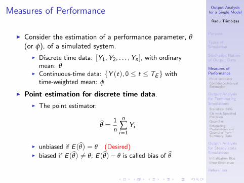
Measures of Performance

I Consider the estimation of a performance parameter, θ(or φ), of a simulated system.

I Discrete time data: [Y1, Y2, . . . , Yn], with ordinarymean: θ

I Continuous-time data: {Y (t), 0 ≤ t ≤ TE } withtime-weighted mean: φ

I Point estimation for discrete time data.

I The point estimator:

θ =1

n

n

∑i=1

Yi

I unbiased if E (θ) = θ (Desired)I biased if E (θ) 6= θ; E (θ)− θ is called bias of θ


Radu Trımbitas

Purpose

Types ofSimulation



Point estimator



Statistical BKG


Quantiles



Initialization Bias

Error Estimation

References

Point estimator I

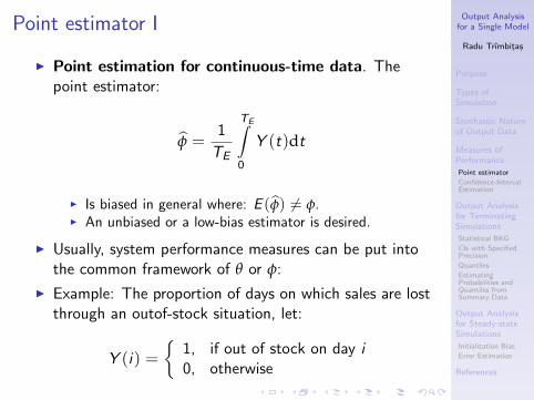
I Point estimation for continuous-time data. Thepoint estimator:

φ =1

TE

TE∫0

Y (t)dt

I Is biased in general where: E (φ) 6= φ.I An unbiased or a low-bias estimator is desired.

I Usually, system performance measures can be put intothe common framework of θ or φ:

I Example: The proportion of days on which sales are lostthrough an outof-stock situation, let:

Y (i) =

{1, if out of stock on day i0, otherwise


Radu Trımbitas

Purpose

Types ofSimulation



Point estimator



Statistical BKG


Quantiles



Initialization Bias

Error Estimation

References

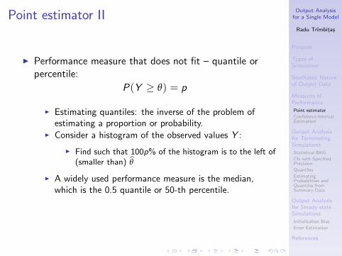
Point estimator II

I Performance measure that does not fit – quantile orpercentile:

P(Y ≥ θ) = p

I Estimating quantiles: the inverse of the problem ofestimating a proportion or probability.

I Consider a histogram of the observed values Y :

I Find such that 100p% of the histogram is to the left of(smaller than) θ

I A widely used performance measure is the median,which is the 0.5 quantile or 50-th percentile.


Radu Trımbitas

Purpose

Types ofSimulation



Point estimator



Statistical BKG


Quantiles



Initialization Bias

Error Estimation

References

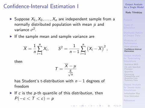
Confidence-Interval Estimation I

I Suppose X1, X2, . . . , Xn are independent sample from anormally distributed population with mean µ andvariance σ2.

I If the sample mean and sample variance are

X =1

n

n

∑i=1

Xi , S2 =1

n− 1

n

∑i=1

(Xi − X

)2,

then

T =X − µ

S√n

has Student‘s t-distribution with n− 1 degrees offreedom

I If c is the p-th quantile of this distribution, thenP(−c < T < c) = p


Radu Trımbitas

Purpose

Types ofSimulation



Point estimator



Statistical BKG


Quantiles



Initialization Bias

Error Estimation

References

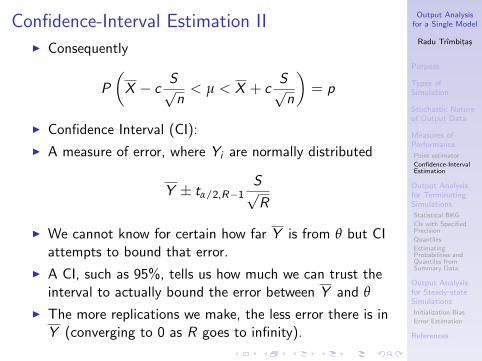
Confidence-Interval Estimation II

I Consequently

P

(X − c

S√n< µ < X + c

S√n

)= p

I Confidence Interval (CI):

I A measure of error, where Yi are normally distributed

Y ± tα/2,R−1S√R

I We cannot know for certain how far Y is from θ but CIattempts to bound that error.

I A CI, such as 95%, tells us how much we can trust theinterval to actually bound the error between Y and θ

I The more replications we make, the less error there is inY (converging to 0 as R goes to infinity).


Radu Trımbitas

Purpose

Types ofSimulation



Point estimator



Statistical BKG


Quantiles



Initialization Bias

Error Estimation

References

Confidence-Interval Estimation III

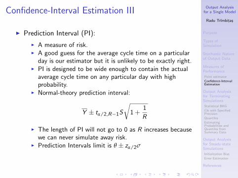
I Prediction Interval (PI):

I A measure of risk.I A good guess for the average cycle time on a particular

day is our estimator but it is unlikely to be exactly right.I PI is designed to be wide enough to contain the actual

average cycle time on any particular day with highprobability.

I Normal-theory prediction interval:

Y ± tα/2,R−1S

√1 +

1

R

I The length of PI will not go to 0 as R increases becausewe can never simulate away risk.

I Prediction Intervals limit is θ ± zα/2σ


Radu Trımbitas

Purpose

Types ofSimulation



Point estimator



Statistical BKG


Quantiles



Initialization Bias

Error Estimation

References

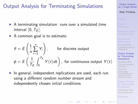
Output Analysis for Terminating Simulations

I A terminating simulation: runs over a simulated timeinterval [0, TE ].

I A common goal is to estimate:

θ = E

(1

n

n

∑i=1

Yi

), for discrete output

φ = E

(1

TE

∫ TE

0Y (t)dt

), for continuous output Y (t)

I In general, independent replications are used, each runusing a different random number stream andindependently chosen initial conditions.


Radu Trımbitas

Purpose

Types ofSimulation



Point estimator



Statistical BKG


Quantiles



Initialization Bias

Error Estimation

References

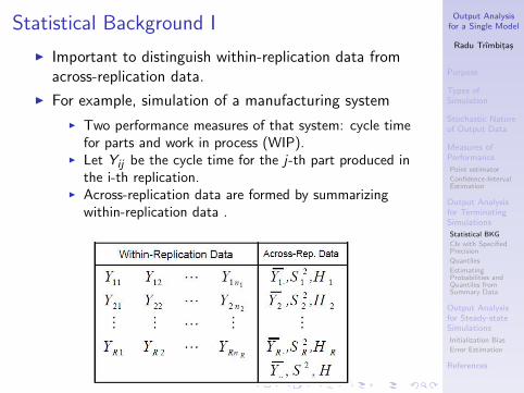
Statistical Background I

I Important to distinguish within-replication data fromacross-replication data.

I For example, simulation of a manufacturing system

I Two performance measures of that system: cycle timefor parts and work in process (WIP).

I Let Yij be the cycle time for the j-th part produced inthe i-th replication.

I Across-replication data are formed by summarizingwithin-replication data .


Radu Trımbitas

Purpose

Types ofSimulation



Point estimator



Statistical BKG


Quantiles



Initialization Bias

Error Estimation

References

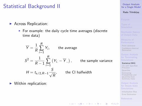
Statistical Background II

I Across Replication:

I For example: the daily cycle time averages (discretetime data)

Y =1

R

R

∑i=1

Yi , the average

S2 =1

R − 1

R

∑i=1

(Yi . − Y ..

), the sample variance

H = tα/2,R−1S√R

, the CI halfwidth

I Within replication:


Radu Trımbitas

Purpose

Types ofSimulation



Point estimator



Statistical BKG


Quantiles



Initialization Bias

Error Estimation

References

Statistical Background III

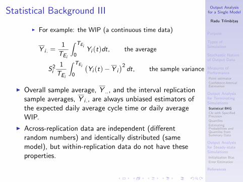
I For example: the WIP (a continuous time data)

Y i . =1

TEi

∫ TEi

0Yi (t)dt, the average

S2i

1

TEi

∫ TEi

0

(Yi (t)− Y i

)2dt, the sample variance

I Overall sample average, Y .., and the interval replicationsample averages, Y i ., are always unbiased estimators ofthe expected daily average cycle time or daily averageWIP.

I Across-replication data are independent (differentrandom numbers) and identically distributed (samemodel), but within-replication data do not have theseproperties.


Radu Trımbitas

Purpose

Types ofSimulation



Point estimator



Statistical BKG


Quantiles



Initialization Bias

Error Estimation

References

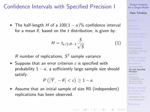
Confidence Intervals with Specified Precision I

I The half-length H of a 100(1− α)% confidence intervalfor a mean θ, based on the t distribution, is given by:

H = tα/2,R−1S√S

(1)

R number of replications, S2 sample variance

I Suppose that an error criterion ε is specified withprobability 1− α, a sufficiently large sample size shouldsatisfy:

P(∣∣Y .. − θ

∣∣ < ε)≥ 1− α

I Assume that an initial sample of size R0 (independent)replications has been observed.


Radu Trımbitas

Purpose

Types ofSimulation



Point estimator



Statistical BKG


Quantiles



Initialization Bias

Error Estimation

References

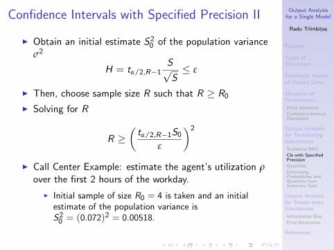
Confidence Intervals with Specified Precision II

I Obtain an initial estimate S20 of the population variance

σ2

H = tα/2,R−1S√S≤ ε

I Then, choose sample size R such that R ≥ R0

I Solving for R

R ≥(

tα/2,R−1S0

ε

)2

I Call Center Example: estimate the agent’s utilization ρover the first 2 hours of the workday.

I Initial sample of size R0 = 4 is taken and an initialestimate of the population variance isS2

0 = (0.072)2 = 0.00518.


Radu Trımbitas

Purpose

Types ofSimulation



Point estimator



Statistical BKG


Quantiles



Initialization Bias

Error Estimation

References

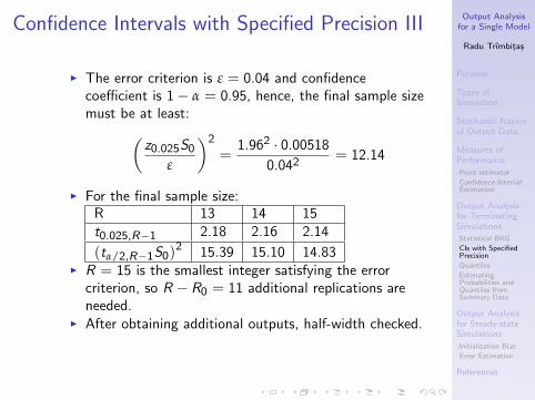
Confidence Intervals with Specified Precision III

I The error criterion is ε = 0.04 and confidencecoefficient is 1− α = 0.95, hence, the final sample sizemust be at least:(

z0.025S0

ε

)2

=1.962 · 0.00518

0.042= 12.14

I For the final sample size:R 13 14 15t0.025,R−1 2.18 2.16 2.14

(tα/2,R−1S0)2 15.39 15.10 14.83

I R = 15 is the smallest integer satisfying the errorcriterion, so R − R0 = 11 additional replications areneeded.

I After obtaining additional outputs, half-width checked.


Radu Trımbitas

Purpose

Types ofSimulation



Point estimator



Statistical BKG


Quantiles



Initialization Bias

Error Estimation

References

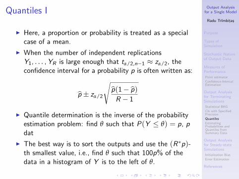
Quantiles I

I Here, a proportion or probability is treated as a specialcase of a mean.

I When the number of independent replicationsY1, . . . , YR is large enough that tα/2,n−1 ≈ zα/2, theconfidence interval for a probability p is often written as:

p ± zα/2

√p(1− p)

R − 1

I Quantile determination is the inverse of the probabilityestimation problem: find θ such that P(Y ≤ θ) = p, pdat

I The best way is to sort the outputs and use the (R∗p)-th smallest value, i.e., find θ such that 100p% of thedata in a histogram of Y is to the left of θ.


Radu Trımbitas

Purpose

Types ofSimulation



Point estimator



Statistical BKG


Quantiles



Initialization Bias

Error Estimation

References

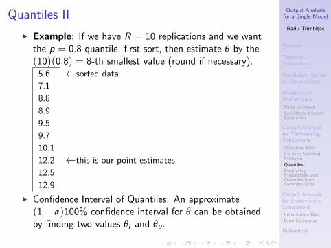
Quantiles II

I Example: If we have R = 10 replications and we wantthe p = 0.8 quantile, first sort, then estimate θ by the(10)(0.8) = 8-th smallest value (round if necessary).

5.6 ←sorted data

7.1

8.8

8.9

9.5

9.7

10.1

12.2 ←this is our point estimates

12.5

12.9

I Confidence Interval of Quantiles: An approximate(1− α)100% confidence interval for θ can be obtainedby finding two values θl and θu.


Radu Trımbitas

Purpose

Types ofSimulation



Point estimator



Statistical BKG


Quantiles



Initialization Bias

Error Estimation

References

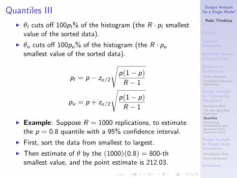
Quantiles III

I θl cuts off 100pl% of the histogram (the R · pl smallestvalue of the sorted data).

I θu cuts off 100pu% of the histogram (the R · pu

smallest value of the sorted data).

pl = p − zα/2

√p(1− p)

R − 1

pu = p + zα/2

√p(1− p)

R − 1

I Example: Suppose R = 1000 replications, to estimatethe p = 0.8 quantile with a 95% confidence interval.

I First, sort the data from smallest to largest.

I Then estimate of θ by the (1000)(0.8) = 800-thsmallest value, and the point estimate is 212.03.


Radu Trımbitas

Purpose

Types ofSimulation



Point estimator



Statistical BKG


Quantiles



Initialization Bias

Error Estimation

References

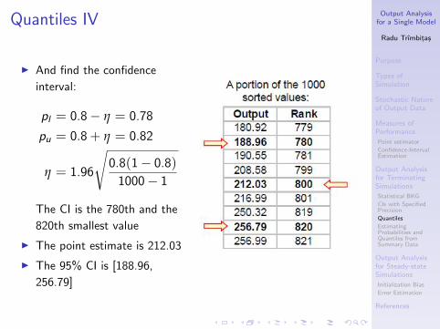
Quantiles IV

I And find the confidence

interval:

pl = 0.8− η = 0.78

pu = 0.8 + η = 0.82

η = 1.96

√0.8(1− 0.8)

1000− 1

The CI is the 780th and the

820th smallest value

I The point estimate is 212.03

I The 95% CI is [188.96,

256.79]


Radu Trımbitas

Purpose

Types ofSimulation



Point estimator



Statistical BKG


Quantiles



Initialization Bias

Error Estimation

References

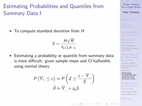
Estimating Probabilities and Quantiles fromSummary Data I

I To compute standard deviation from H

S =H√

R

tα/2,R−1

I Estimating a probability or quantile from summary datais more difficult: given sample mean and CI halfwidth,using normal theory

P(Y i . ≤ c

)≈ P

(Z ≤ c − Y ..

S

)θ ≈ Y .. + zpS


Radu Trımbitas

Purpose

Types ofSimulation



Point estimator



Statistical BKG


Quantiles



Initialization Bias

Error Estimation

References

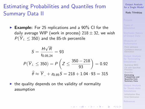
Estimating Probabilities and Quantiles fromSummary Data II

I Example: For 25 replications and a 90% CI for thedaily average WIP (work in process) 218± 32, we wishP(Y i . ≤ 350) and the 85-th percentile

S =H√

R

t0.05,24= 93

P(Y i . ≤ 350) = P

(Z ≤ 350− 218

93

)= 0.92

θ ≈ Y .. + z0.85S = 218 + 1.04 · 93 = 315

I the quality depends on the validity of normalityassumption


Radu Trımbitas

Purpose

Types ofSimulation



Point estimator



Statistical BKG


Quantiles



Initialization Bias

Error Estimation

References

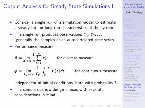
Output Analysis for Steady-State Simulations I

I Consider a single run of a simulation model to estimatea steadystate or long-run characteristics of the system.

I The single run produces observations Y1, Y2, . . .(generally the samples of an autocorrelated time series).

I Performance measure:

θ = limn→∞

1

n

n

∑i=1

Yi , for discrete measure

φ = limTE→∞

1

TE

∫ TE

0Y (t)dt, for continuous measure

independent of initial conditions, both with probability 1

I The sample size is a design choice, with severalconsiderations in mind:


Radu Trımbitas

Purpose

Types ofSimulation



Point estimator



Statistical BKG


Quantiles



Initialization Bias

Error Estimation

References

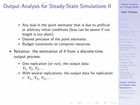
Output Analysis for Steady-State Simulations II

I Any bias in the point estimator that is due to artificialor arbitrary initial conditions (bias can be severe if runlength is too short).

I Desired precision of the point estimator.I Budget constraints on computer resources.

I Notation: the estimation of θ from a discrete-timeoutput process.

I One replication (or run), the output data:Y1, Y2, Y3, . . .

I With several replications, the output data for replicationr : Yr1 , Yr2 , Yr3 , . . .


Radu Trımbitas

Purpose

Types ofSimulation



Point estimator



Statistical BKG


Quantiles



Initialization Bias

Error Estimation

References

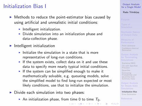
Initialization Bias I

I Methods to reduce the point-estimator bias caused byusing artificial and unrealistic initial conditions:

I Intelligent initialization.I Divide simulation into an initialization phase and

data-collection phase.

I Intelligent initialization

I Initialize the simulation in a state that is morerepresentative of long-run conditions.

I If the system exists, collect data on it and use thesedata to specify more nearly typical initial conditions.

I If the system can be simplified enough to make itmathematically solvable, e.g. queueing models, solvethe simplified model to find long-run expected or mostlikely conditions, use that to initialize the simulation.

I Divide each simulation into two phases:

I An initialization phase, from time 0 to time T0.


Radu Trımbitas

Purpose

Types ofSimulation



Point estimator



Statistical BKG


Quantiles



Initialization Bias

Error Estimation

References

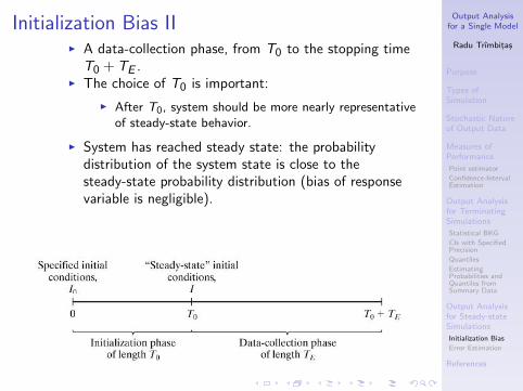
Initialization Bias III A data-collection phase, from T0 to the stopping time

T0 + TE .I The choice of T0 is important:

I After T0, system should be more nearly representativeof steady-state behavior.

I System has reached steady state: the probabilitydistribution of the system state is close to thesteady-state probability distribution (bias of responsevariable is negligible).


Radu Trımbitas

Purpose

Types ofSimulation



Point estimator



Statistical BKG


Quantiles



Initialization Bias

Error Estimation

References

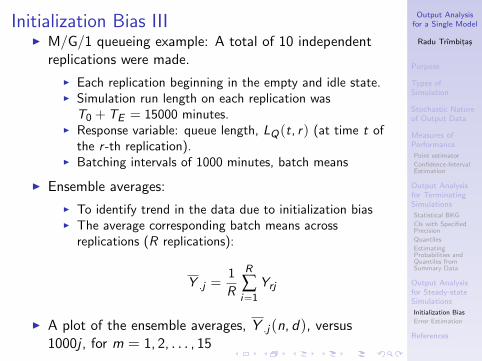
Initialization Bias IIII M/G/1 queueing example: A total of 10 independent

replications were made.

I Each replication beginning in the empty and idle state.I Simulation run length on each replication was

T0 + TE = 15000 minutes.I Response variable: queue length, LQ(t, r) (at time t of

the r -th replication).I Batching intervals of 1000 minutes, batch means

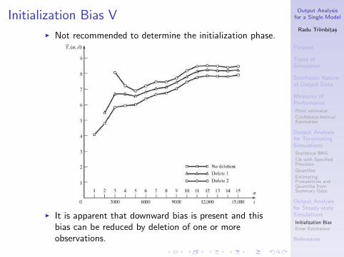
I Ensemble averages:

I To identify trend in the data due to initialization biasI The average corresponding batch means across

replications (R replications):

Y .j =1

R

R

∑i=1

Yrj

I A plot of the ensemble averages, Y .j (n, d), versus1000j , for m = 1, 2, . . . , 15


Radu Trımbitas

Purpose

Types ofSimulation



Point estimator



Statistical BKG


Quantiles



Initialization Bias

Error Estimation

References

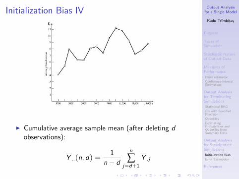
Initialization Bias IV

I Cumulative average sample mean (after deleting dobservations):

Y ..(n, d) =1

n− d

n

∑j=d+1

Y .j


Radu Trımbitas

Purpose

Types ofSimulation



Point estimator



Statistical BKG


Quantiles



Initialization Bias

Error Estimation

References

Initialization Bias V

I Not recommended to determine the initialization phase.

I It is apparent that downward bias is present and thisbias can be reduced by deletion of one or moreobservations.


Radu Trımbitas

Purpose

Types ofSimulation



Point estimator



Statistical BKG


Quantiles



Initialization Bias

Error Estimation

References

Initialization Bias VI

I No widely accepted, objective and proven technique toguide how much data to delete to reduce initializationbias to a negligible level.

I Plots can, at times, be misleading but they are stillrecommended.

I Ensemble averages reveal a smoother and more precisetrend as the number of replications, R, increases.

I Ensemble averages can be smoothed further by plottinga moving average.

I Cumulative average becomes less variable as more dataare averaged.

I The more correlation present, the longer it takes for toapproach steady state Y .j

I Different performance measures could approach steadystate at different rates.


Radu Trımbitas

Purpose

Types ofSimulation



Point estimator



Statistical BKG


Quantiles



Initialization Bias

Error Estimation

References

Error Estimation I

I If {Y1, . . . , Yn} are not statistically independent, thenS2/n is a biased estimator of the true variance.

I Almost always the case when {Y1, . . . , Yn} is asequence of output observations from within a singlereplication (autocorrelated sequence, time-series).

I Suppose the point estimator θ is the sample mean

Y =1

n

n

∑i=1

Yi

I Variance of Y is very hard to estimate.

I For systems with steady state, produce an outputprocess that is approximately covariance stationary(after passing the transient phase).


Radu Trımbitas

Purpose

Types ofSimulation



Point estimator



Statistical BKG


Quantiles



Initialization Bias

Error Estimation

References

Error Estimation II

I The covariance between two random variables in thetime series depends only on the lag, i.e. the number ofobservations between them.

I For a covariance stationary time series, {Y1, . . . , Yn}:I Lag-k autocovariance is:

γk = cov(Y1, Y1+k ) = cov(Yi , Yi+k )I Lag-k autocorrelation is: ρk = γk

σ2 , −1 ≤ ρk ≤ 1

I If a time series is covariance stationary, then thevariance of Y is:

V (Y ) =σ2

n

1 + 2n−1

∑k=1

(1− k

n

)ρk︸︷︷︸

c


Radu Trımbitas

Purpose

Types ofSimulation



Point estimator



Statistical BKG


Quantiles



Initialization Bias

Error Estimation

References

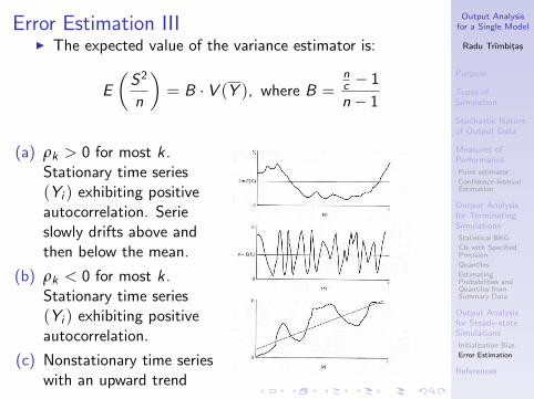
Error Estimation IIII The expected value of the variance estimator is:

E

(S2

n

)= B · V (Y ), where B =

nc − 1

n− 1

(a) ρk > 0 for most k.Stationary time series(Yi ) exhibiting positiveautocorrelation. Serieslowly drifts above andthen below the mean.

(b) ρk < 0 for most k .Stationary time series(Yi ) exhibiting positiveautocorrelation.

(c) Nonstationary time serieswith an upward trend


Radu Trımbitas

Purpose

Types ofSimulation



Point estimator



Statistical BKG


Quantiles



Initialization Bias

Error Estimation

References

Error Estimation IV

I The expected value of the variance estimator is:

E

(S2

n

)= B · V (Y ),

where B = n/c−1n−1 , and V (Y ) is the variance of Y .

I If (Yi ) are independent, then S2/n is an unbiasedestimator of V (Y )

I If the autocorrelation ρk are primarily positive, thenS2/n is biased low as an estimator of V (Y ).

I If the autocorrelation ρk are primarily negative, thenS2/n is biased high as an estimator of V (Y ).


Radu Trımbitas

Purpose

Types ofSimulation



Point estimator



Statistical BKG


Quantiles



Initialization Bias

Error Estimation

References

Replication Method I

I Use to estimate point-estimator variability and toconstruct a confidence interval.

I Approach: make R replications, initializing and deletingfrom each one the same way.

I Important to do a thorough job of investigating theinitial-condition bias:

I Bias is not affected by the number of replications,instead, it is affected only by deleting more data (i.e.,increasing T0) or extending the length of each run (i.e.increasing TE ).

I Basic raw output data {Yrj , r = 1, . . . , R, j = 1, . . . , n}is derived by:

I Individual observation from within replication r .I Batch mean from within replication r of some number

of discrete-time observations.


Radu Trımbitas

Purpose

Types ofSimulation



Point estimator



Statistical BKG


Quantiles



Initialization Bias

Error Estimation

References

Replication Method II

I Batch mean of a continuous-time process over timeinterval j .

I Each replication is regarded as a single sample forestimating θ. For replication r:

Y r .(n, d) =1

n− d

n

∑j=d+1

Yrj

I The overall point estimator:

Y ..(n, d) =1

R

r

∑r=1

Y r .(n, d) and E[Y ..(n, d)

]= θnd

I If d and n are chosen sufficiently large:

I θnd ≈ θI Y ..(n, d) is an approximately unbiased estimator of θ.


Radu Trımbitas

Purpose

Types ofSimulation



Point estimator



Statistical BKG


Quantiles



Initialization Bias

Error Estimation

References

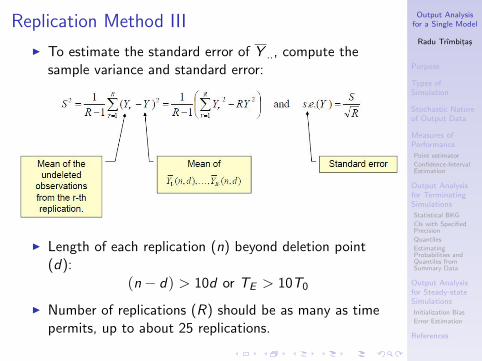
Replication Method III

I To estimate the standard error of Y .., compute thesample variance and standard error:

I Length of each replication (n) beyond deletion point(d):

(n− d) > 10d or TE > 10T0

I Number of replications (R) should be as many as timepermits, up to about 25 replications.


Radu Trımbitas

Purpose

Types ofSimulation



Point estimator



Statistical BKG


Quantiles



Initialization Bias

Error Estimation

References

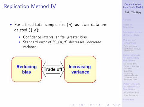
Replication Method IV

I For a fixed total sample size (n), as fewer data aredeleted (↓ d):

I Confidence interval shifts: greater bias.I Standard error of Y ..(n, d) decreases: decrease

variance.


Radu Trımbitas

Purpose

Types ofSimulation



Point estimator



Statistical BKG


Quantiles



Initialization Bias

Error Estimation

References

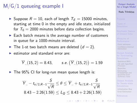
M/G/1 queueing example I

I Suppose R = 10, each of length TE = 15000 minutes,starting at time 0 in the empty and idle state, initializedfor T0 = 2000 minutes before data collection begins.

I Each batch means is the average number of customersin queue for a 1000-minute interval.

I The 1-st two batch means are deleted (d = 2).

I estimator and standard error are:

Y ..(15, 2) = 8.43, s.e.(Y ..(15, 2)

)= 1.59

I The 95% CI for long-run mean queue length is:

Y .. − tα/2,R−1S√R≤ θ ≤ Y .. + tα/2,R−1

S√R

8.43− 2.26(1.59) ≤ LQ ≤ 8.43 + 2.26(1.59)


Radu Trımbitas

Purpose

Types ofSimulation



Point estimator



Statistical BKG


Quantiles



Initialization Bias

Error Estimation

References

M/G/1 queueing example II

I A high degree of confidence that the long-run meanqueue length is between 4.84 and 12.02 (if d and n are“large” enough).


Radu Trımbitas

Purpose

Types ofSimulation



Point estimator



Statistical BKG


Quantiles



Initialization Bias

Error Estimation

References

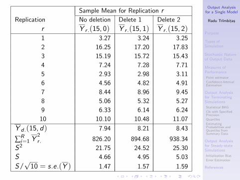
Sample Mean for Replication rReplication No deletion Delete 1 Delete 2

r Y r .(15, 0) Y r .(15, 1) Y r .(15, 2)1 3.27 3.24 3.25

2 16.25 17.20 17.83

3 15.19 15.72 15.43

4 7.24 7.28 7.71

5 2.93 2.98 3.11

6 4.56 4.82 4.91

7 8.44 8.96 9.45

8 5.06 5.32 5.27

9 6.33 6.14 6.24

10 10.10 10.48 11.07

Y d .(15, d) 7.94 8.21 8.43

∑Ri=1 Y

2r . 826.20 894.68 938.34

S2 21.75 24.52 25.30

S 4.66 4.95 5.03

S/√

10 = s.e.(Y ) 1.47 1.57 1.59


Radu Trımbitas

Purpose

Types ofSimulation



Point estimator



Statistical BKG


Quantiles



Initialization Bias

Error Estimation

References

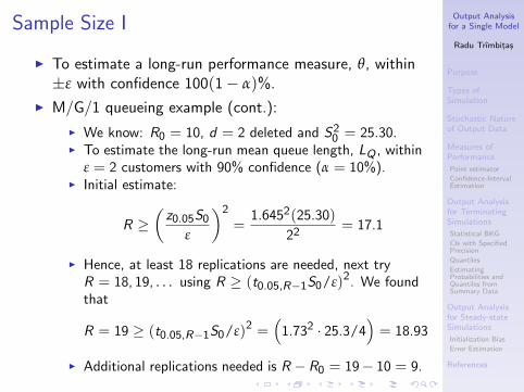
Sample Size I

I To estimate a long-run performance measure, θ, within±ε with confidence 100(1− α)%.

I M/G/1 queueing example (cont.):

I We know: R0 = 10, d = 2 deleted and S20 = 25.30.

I To estimate the long-run mean queue length, LQ , withinε = 2 customers with 90% confidence (α = 10%).

I Initial estimate:

R ≥(

z0.05S0

ε

)2

=1.6452(25.30)

22= 17.1

I Hence, at least 18 replications are needed, next tryR = 18, 19, . . . using R ≥ (t0.05,R−1S0/ε)2. We foundthat

R = 19 ≥ (t0.05,R−1S0/ε)2 =(

1.732 · 25.3/4)= 18.93

I Additional replications needed is R −R0 = 19− 10 = 9.


Radu Trımbitas

Purpose

Types ofSimulation



Point estimator



Statistical BKG


Quantiles



Initialization Bias

Error Estimation

References

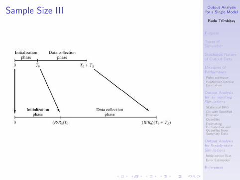
Sample Size II

I An alternative to increasing R is to increase total runlength T0 + TE within each replication.

I Approach:

I Increase run length from T0 +TE to(R/R0)(T0 +TE ), and

I Delete additional amount of data, from time 0 to time(R/R0)T0.

I Advantage: any residual bias in the point estimatorshould be further reduced.

I However, it is necessary to have saved the state of themodel at time T0 + TE and to be able to restart themodel.


Radu Trımbitas

Purpose

Types ofSimulation



Point estimator



Statistical BKG


Quantiles



Initialization Bias

Error Estimation

References

Sample Size III


Radu Trımbitas

Purpose

Types ofSimulation



Point estimator



Statistical BKG


Quantiles



Initialization Bias

Error Estimation

References

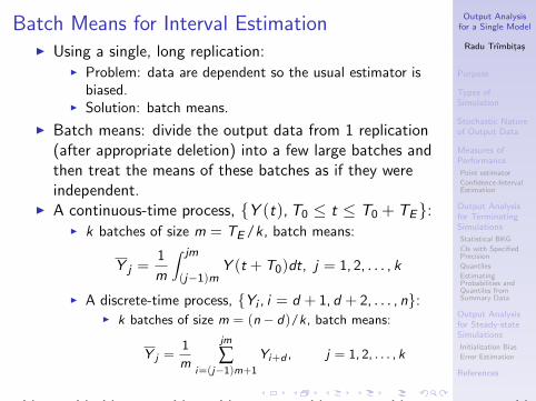
Batch Means for Interval EstimationI Using a single, long replication:

I Problem: data are dependent so the usual estimator isbiased.

I Solution: batch means.

I Batch means: divide the output data from 1 replication(after appropriate deletion) into a few large batches andthen treat the means of these batches as if they wereindependent.

I A continuous-time process, {Y (t), T0 ≤ t ≤ T0 + TE}:I k batches of size m = TE/k , batch means:

Y j =1

m

∫ jm

(j−1)mY (t + T0)dt, j = 1, 2, . . . , k

I A discrete-time process, {Yi , i = d + 1, d + 2, . . . , n}:I k batches of size m = (n− d)/k, batch means:

Y j =1

m

jm

∑i=(j−1)m+1

Yi+d , j = 1, 2, . . . , k

Y1, . . . , Yd︸︷︷︸deleted

, Yd+1, . . . , Yd+m︸︷︷︸Y 1

, Yd+m+1, . . . , Yd+2m︸︷︷︸Y 2

, . . . , Yd+(k−1)m+1, . . . , Yd+km︸︷︷︸Ym

I Starting either with continuous-time or discrete-timedata, the variance of the sample mean is estimated by:

S2

k=

1

k

k

∑j=1

(Y j − Y

)2

k − 1=

k

∑j=1

Y2j − kY

2

k (k − 1)

I If the batch size is sufficiently large, successive batchmeans will be approximately independent, and thevariance estimator will be approximately unbiased.

I No widely accepted and relatively simple method forchoosing an acceptable batch size m. Some simulationsoftware does itautomatically.


Radu Trımbitas

Purpose

Types ofSimulation



Point estimator



Statistical BKG


Quantiles



Initialization Bias

Error Estimation

References

Summary

I Stochastic discrete-event simulation is a statisticalexperiment.

I Purpose of statistical experiment: obtain estimates ofthe performance measures of the system.

I Purpose of statistical analysis: acquire some assurancethat these estimates are sufficiently precise.

I Distinguish: terminating simulations and steady-statesimulations.

I Steady-state output data are more difficult to analyze

I Decisions: initial conditions and run lengthI Possible solutions to bias: deletion of data and

increasing run length

I Statistical precision of point estimators are estimated bystandard-error or confidence interval

I Method of independent replications was emphasized.

I Batch mean for a long run replication


Radu Trımbitas

Purpose

Types ofSimulation



Point estimator



Statistical BKG


Quantiles



Initialization Bias

Error Estimation

References

References

Averill M. Law, Simulation Modeling and Analysis,McGraw-Hill, 2007

J. Banks, J. S. Carson II, B. L. Nelson, D. M. Nicol,Discrete-Event System Simulation, Prentice Hall, 2005

J. Banks (ed), Handbook of Simulation, Wiley, 1998,Chapter 11

Documents

Radu Tr^ mbit˘a˘s Purpose Simulation Output Analysis for a ...math.ubbcluj.ro/~tradu/OutputDataAnal.pdf · Output Analysis for a Single Model Radu Tr^ mbit˘a˘s Purpose Types of