Rail Network Detection from Aerial Imagery using Deep Learning

Mehrdad SalehiApple Inc

msalehi@stanford.edu

Yonghong WangApple Inc

yhwang99@stanford.edu

Abstract

Having an accurate and up-to-date rail network data isthe foundation of any mapping application that supportspublic transportation. Traditionally, creating such a net-work needs manual digitization of satellite imagery andbuilding the network with human intervention. The goalof this project is to segment the rail network from aerialimagery using Deep Learning. In this project, we studydifferent techniques to classify and segment rail networksin the aerial imagery. We implement ConvNets as well ascombination of ConvNets and DeConvNets to classify andsegment the rail network. We also share the insights that wederived from analyzing the results.

1. Introduction

Having an accurate and up-to-date rail network data isthe foundation of any mapping application that supportspublic transportation. Traditionally, creating such a networkneeds manual digitization of satellite imagery and involveshuman intervention. The goal of this project is to segmentthe rail network from aerial imagery using Deep Learning.This project has three main contributions: First, we classi-fied images into two classes of rail and non-rail using a net-work of 7 ConvNets and three fully connected nets; secondwe did a coarse-level segmentation using ConvNets by re-ducing dimensionality of images to the label space, we alsoimproved the results dramatically by using ConvNets andDeConvNets, and finally we did a fine-level segmentationby using ConvNets and DeConvNets.

2. Data Preparation

For this project, we needed both aerial imagery and la-bel dataset. Aerial imagery data can be downloaded fromproviders such as USGS. For label dataset, we used anopen source mapping data platform called Open Street Map(OSM) where we obtained labels for our learning algorithmas well as for evaluation.

Figure 1. Example of images, two top images do not have railtrack, two bottom images have rail tracks in them

2.1. Aerial Imagery

Aerial imagery should be converted to tiles so that theinput data have a uniform size. We followed a standardtiling systems used in the mapping industry. The imagesize for classification and coarse segmentation are 60x60meters. For the fine segmentation, we used 30x30 meterimages as the data instance. As for the pixel size, in coarsesegmentation, each pixel is 3.5x3.5 meters, while for thefine segmentation we used the actual pixel of the image thatis about 10cm.

2.2. Label Dataset

In order to prepare the labels we processed OSM rail net-work for the entire USA. We used Spark, Scala, and JTS andran our Spark job on a cluster of machines. For the 3.5x3.5meter tiles, it took about one hour to create the label tiles.This time was longer for 10cm labels, as we used a differ-ent technique using Python on a single machine. Figure 1shows some examples in the dataset.

1

3. Related WorkWe used neural network to classify and segment rail net-

work from satellite images. So we first discuss the workon image classification and segmentation. Image classifica-tion is the task of assigning one label to each input imagefrom a fixed set of categories. Krizhevsky et al., in [7] usedConvNets and dropout ( 5 layer CNNs and 3 layer fully con-nected layers), and achieved 15.3% top-5 test error rate inILSVRC 2010 challenge which is significantly better than26.2% top-5 test error rate by the 2nd place. This marks theturning point for large-scale object recognition, and sincethen deep neural networks outperforms traditional machinelearning methods. Simonyan et al., in [16] further improvedthe top-5 test error rate to 6.8%. They used deep and narrowCNN filters (14 CNN layers, 3 FC layers). Szegedy et al.,in [17] introduced GoogLeNet, a 22 layers deep networkwith efficient inception module and no FC layers. Theyachieved 6.7 % top 5 erorr and won 2014 ILSVRC chal-lenge. In 2015, [4], He et al., proposed Residual Networkand improved the top-5 test error to 3.57% and surpasseshuman performance. Using Residual Network, they can usevery deep network (152 layers). Zagoruyko et al., in [18]introduced wide residual networks (WRNs) and show thatthey are far superior than deep residual networks in both ef-ficiency and accuracy. They achieved new state-of-the-artresults on CIFAR, SVHN, COCO and significant improve-ments on ImageNet.

Image segmentation is the task of partitioning image intomultiple segments, and each segment belongs to one cat-egory. Pohlen et al., in [14] proposed a network archi-tecture for semantic segmentation in street scenes. It usedResNet encoder/decoder architecture and residuals remainat the full input resolution throughout the network. He etal., in [3] introducted Mask R-CNN method to efficientlydetect objects in an image and generate high-quality seg-mentation mask for each object. They extends Faster R-CNN method, [15], by adding a branch for predicting anobject mask at the same time. Mask R-CNN outperformsall exsisting, single-model entries on every task, and wonCOCO 2016 challeng.

Mnih et al., in [13] proposed a large-scale learning ap-proach to detecting roads using a neural network. Theyused much larger labelled datasets, and introduced a post-processing method to significantly improve the results. In-stead of predicting each pixel is road or not, they predicta small block of pixels is road or not, and they are ableto get around 87% test accuracy. Acar et al., in [19] us-ing classification algorithms to detect road from satelite im-ages. They used a method consisting of two stages. Theyfirst preprocess the image by using greyscale transformationand thresholding process and obtained a binary image, thenthey use K-nearest neighbours and Naive Bayes classifierson images by using colour features. They got around 70%

to 80 % recall and about 33% to 40 % precision in detectingif 15 x 15 pixel block is part of a road. Kahraman et al., in[6] studied road detection from satellite images using neuralnetworks. The used Multilayer Perceptron (multilayer neu-ral network). For every pixel, they used 27 features from 3x 3 x 3 pixels around it, and predict if the pixel is part of aroad. They were able to get accuracy between 87% and 93%for different settings. Maboudi et al., in [9] introduced amulti-stage object-based approach for road extraction fromVHR satellite images. They use Edge-preserving guided fil-tering to improve the segmentation quality. They also pro-posed a skeleton based linearity index called SOLI. Theyhave achieved more than 84% accuracy for the datasets theystudied. Marmanis et al., in [12], proposed a deep learningapproach to semantic segmentation of high resolution aerialimages. They used Fully Convolution Networks (FCNs)and aggressive deconvolution with recycling of early net-work layers, and finally converted into a pixelwise classifi-cation at full resolution. They achieved 86% accuracy ontheir dataset.

They are very few research in detecting and segmentingrail network from satellige images. Maqsood et al., in [11]developed an algorithm to detect railway track from imagestaken from Google maps. They studied only a small regioninstead of whole state, country or world. They combinededge detection and line detection algorithms to detect rail-way.

To make deep neural network work, tuning hyper param-eters places a crutial role. Bengio in [1], discussed varioustechniques to train deep neural network and tune hyper pa-rameters.

4. Aerial Image Classification

The goal of this part of the project was to classifywhether a satellite image contains a rail track or not. Theclassifier should discriminate an image that contains a railtrack from other ones. The input image is a 256 x 256 x 3where each image tile is 60m x 60m. We are interested toget a label for each tile whether it contains a rail track ornot.

4.1. Network Architecture

We implemented a 10 layer convolutional neural networkwith 7 ConvNets and 3 fully connected networks. Aftereach ConvNet (except the last one), we applied a max pool-ing layer. Also, we applied a batch normalization layer aftereach layer. Table 1 summarizes the architecture of the net-work.

4.2. Training and Hyper Parameter Tuning

We trained a network with 7 convolutional layers and 3fully connected layers (See Table 1). First we tried larger

2

Layer SizeConv 1 3 x 3 x 96Max-pooling 2 x 2Conv 2 3 x 3 x 128Max-pooling 2 x 2Conv 3 3 x 3 x 192Max-pooling 2 x 2Conv 4 3 x 3 x 192Max-pooling 2 x 2Conv 5 3 x 3 x 128Max-pooling 2 x 2Conv 6 3 x 3 x 128Max-pooling 2 x 2Conv 7 3 x 3 x 128FC 1 128 x 128FC 2 128 x 64FC 3 64 x 2

Table 1. Network architecture for image classification

number of channels (e.g., 1024), but training on this net-work was slow and even crashed because of insufficientmemory. Then we reduced the number of channels from1024 to 192 or 128. This enabled us to train the model. Ex-cept for the last one, after each convolutional layer we useda max-pooling layer to reduce the dimensionality. Also, weapplied a batch normalization layer after each convolutionallayer. The ReLu non-linearity was applied as the activationfunction.

At the first run, we had a small training dataset consist-ing of ten thousand images. Using these images we trainedthe network and obtained 84% accuracy on the test dataset.Then we created more labels of around 100 thousand im-ages and also added learning rate decay to the model withstep size 1000 and decay of 0.96. We trained the model withother decay rates and steps sizes (e.g., step size of 10000and decay 0.1 and also step size 1000 with decay 0.5). Fi-nally, the best accuracy that we obtained on the test set after1 epoch was 96%. At the end, we increased the number ofepochs to 5 and as a result we obtained 98% accuracy onthe test set.

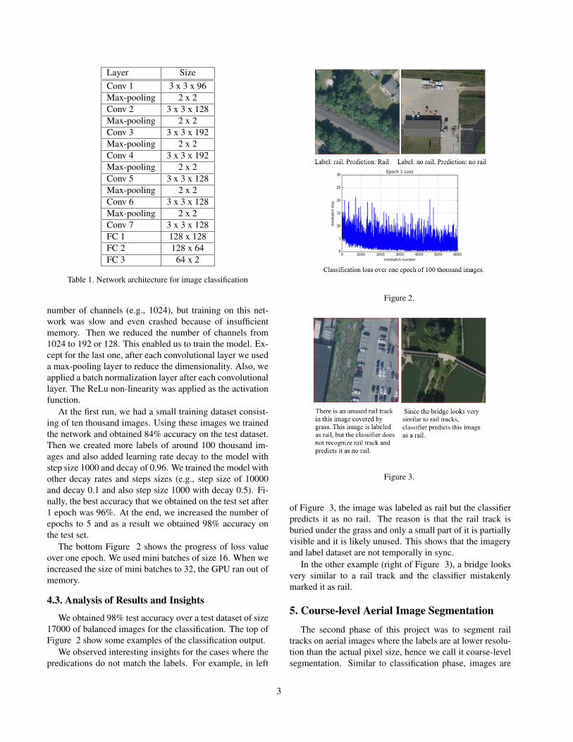
The bottom Figure 2 shows the progress of loss valueover one epoch. We used mini batches of size 16. When weincreased the size of mini batches to 32, the GPU ran out ofmemory.

4.3. Analysis of Results and Insights

We obtained 98% test accuracy over a test dataset of size17000 of balanced images for the classification. The top ofFigure 2 show some examples of the classification output.

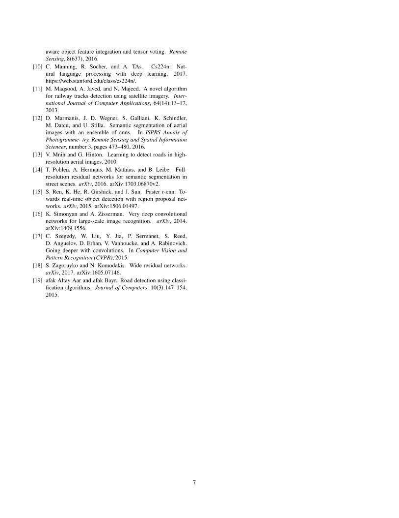
We observed interesting insights for the cases where thepredications do not match the labels. For example, in left

Figure 2.

Figure 3.

of Figure 3, the image was labeled as rail but the classifierpredicts it as no rail. The reason is that the rail track isburied under the grass and only a small part of it is partiallyvisible and it is likely unused. This shows that the imageryand label dataset are not temporally in sync.

In the other example (right of Figure 3), a bridge looksvery similar to a rail track and the classifier mistakenlymarked it as rail.

5. Course-level Aerial Image Segmentation

The second phase of this project was to segment railtracks on aerial images where the labels are at lower resolu-tion than the actual pixel size, hence we call it coarse-levelsegmentation. Similar to classification phase, images are

3

Figure 4.

Layer SizeConv 1 7 x 7 x 96Max-pooling 2 x 2Conv 2 5 x 5 x 128Max-pooling 2 x 2Conv 3 3 x 3 x 128Max-pooling 2 x 2Conv 4 3 x 3 x 256Max-pooling 2 x 2Conv 5 3 x 3 x 128Max-pooling 2 x 2Conv 6 3 x 3 x64Max-pooling 2 x 2Conv 7 1 x 1 x 2

Table 2. ConvNets Network architecture for coarse-level imagesegmentation

60m x 60m aerial images. However, at this phase our goalwas to segment each 3.5m x 3.5m of the image. We used3.5m as the resolution size because we were able to createlarge amount of labels at this resolution. Figures 4 showsthe resolution of labels (red tiles) for a 60m x 60m images.Each image 60m x 60m includes 16 x16 labels.

5.1. Network Architecture

Since each image has 16 x 16 labels, we defined a con-volutional neural network that reduced the dimension of theinput image (256 x 256) to the dimension of labels (16 x16). We defined a network that consists of 7 ConvNets.Table 2 summarizes the network architecture. We also de-fined a DeConvNets, with 15 layers ConvNets, and 8 layersDeConvNets, each layer followed by Batch Normalization.Input is 256 x 256 x 3, output is 16 x 16 x 2. Table 3summarizes the network architecture.

Layer Size StepConv 1 3 x 3 x 32 1Conv 2 3 x 3 x 64 2Conv 3 3 x 3 x 64 1Conv 4 3 x 3 x 128 2Conv 5 3 x 3 x 128 1Conv 6 3 x 3 x 128 1Conv 7 3 x 3 x 256 2Conv 8 3 x 3 x 256 1Conv 9 3 x 3 x 256 1Conv 10 3 x 3 x 256 2Conv 11 3 x 3 x 256 1Conv 12 3 x 3 x 256 1Conv 13 3 x 3 x 256 2Conv 14 8 x 8 x 2048 1Conv 15 1 x 1 x 2048 1DeConv 1 8 x 8 x 256 1 (valid)DeConv 2 3 x 3 x 256 1DeConv 3 3 x 3 x 256 1DeConv 4 3 x 3 x 128 2DeConv 5 3 x 3 x 64 1DeConv 6 3 x 3 x 32 1DeConv 7 3 x 3 x 16 1DeConv 8 3 x 3 x 2 1

Table 3. ConvNets and DeConvNets Network architecture forcoarse-level image segmentation

5.2. Training and Hyper Parameter Tuning

We started training the model with the same images thatwe used to train the classification part (Section 4), but al-most all the image were predicted as no rail. This happenedbecause the data was imbalanced (each negative example ofclassification phase contains no positive pixel but 256 nega-tive ones). Next, we trained using only images that includerail network (removed negative examples). After this up-date, the results were slightly improved but still we weremissing large number of rail tracks. Finally, we includedonly images that, out of 256 coarse labels, have at least30 pixels labeled as rail. This change improved the mod-els performance significantly. We trained the network withmultiple learning rate decays and step sizes. Eventually thefinal hyper parameters were learning rate decay of 0.96 andstep size of 1000. We used 78000 images for training thenetwork.

We trained both networks for two epochs. Figures 5shows the training loss after the first and second epochs.

5.3. Analysis of Results and Insights

For the ConvNets model, coarse-level segmentation, weobtained an overall precision of 85%, recall of 46% and59.7% F1 for the positive examples (rail tracks). For the

4

Figure 5.

Figure 6.

ConvNets and DeConvNets model, coarse-level segmenta-tion, we obtained an overall precision of 84.%, recall of77.8% and 81.0% F1 for the positive examples (rail tracks).We observed interesting insights by analyzing the predic-tions.Figures 6 shows satellite images and predicted labelsfor them. The classifier sometimes gets confused betweenroad and rail network and segment road as rail (Figures 6).This example shows that we might need to add more nega-tive examples including roads.

Figure 7.

Layer SizeConv 1 7 x 7 x 32Max-pooling 2 x 2Conv 2 5 x 5 x 64Max-pooling 2 x 2Conv 3 3 x 3 x 96Conv 4 1 x 1 x 96DeConv 1 3 x 3 x 64DeConv 2 3 x 3 x 32DeConv 3 3 x 3 x 2

Table 4. Network architecture for fine-level image segmentation

6. Fine-level Aerial Image SegmentationThe final phase of this project was to segment rail tracks

at individual pixel level. To make the predictions more ac-curate, we used higher resolution images at this stage whereeach images covers 30 x 30 meter. We created label datasetby intersecting OSM rail tracks with a 30 x 30 meter grid.Figure 7 shows the aerial image overlapping with the gen-erated label from OSM data.

6.1. Network Architecture

We used a mixture of ConvNet-DeConvNet to segmentimages. First we reduced the dimensionality of images from256 x 256 to 32 x 32 using ConNets and then increased di-mensionality from 32 x 32 to 256 x 256 using DeConvNet.Table 4 summarizes the architecture of the network.

6.2. Training and Hyper Parameter Tuning

As the first attempt to train the model, instead of usingthe tick lines covering rail tracks (Figure 7), we used therail tracks centerline (a thin line). However such a dataset ishugely imbalanced. We tried to fix this by using a weightedsoftmax cross entroy loss, and tried different weights foreach dataset. The results were not promising (we got below

5

Figure 8.

10% recall). Keeping the same strategy, we increased theamount of training data from 20000 to 40000 and trainedfor 10 epochs, but the results did not improve.

Finally, we used the training data as tick lines that coverthe entire width of rail tracks (see Figure 7). This strategyimproved the results so that even after the first epoch theclassifier was able to approximately detect rail tracks. Wechanged the learning rate decay and decay step and eventu-ally chose 0.96 and 1000 respectively. Figure 8 show theloss values during epoch 1 and 7.

6.3. Analysis of Results and Insights

For the fine-level segmentation, we obtained an overallprecision of 68% and recall of 70% for the positive exam-ples (rail tracks). By analyzing the prediction results andlabels, we were able to reason about the specific pattern thatwe see in the results.The top of Figure 9 shows an aerial im-agery that contains two rail tracks as well as the predictedresults. Blue indicates predicted rail tracks and the red high-lights no rail pixels. By analyzing the bottom of Figure 9,we can conclude that those parts of rail tracks that were visi-ble in the imagery were detected. However, those parts thatare under the bridge or covered by the trees shadow werenot detected. In addition, the tiny elevated regions on thebridges median that look like the elevated part of rail tracksare predicted as rail.

7. Future WorkAs for the future work, we will use ResNets with DeCon-

vNets, Wide ResNets [18] and Mask R-CNN [3]. We arealso interested in training ensembled networks, and then useDark Knowledge method which was co-invented by Hintonet al., [5], to train a single network based on original labels,and soft labels created by ensembled models.

8. AcknowledgementsWe thank Yi Cao for help with providing some labels

for each pixel of the satellite images at zoom 20 (30m X30m). We also use sample codes from Stanford ComputerVision CS231n course [8], NLP course CS224n [10], andreferenced sample code in Github, [2]

Figure 9.

We are thankful for CS231 teaching stuff for this won-derful class.

References[1] Y. Bengio. Practical recommendations for gradient-

based training of deep architectures. arXiv, 2012.arXiv:1206.5533.

[2] fabianbormann. Tensorflow-deconvnet-segmentation.https://github.com/fabianbormann/Tensorflow-DeconvNet-Segmentation/commits/master.

[3] K. He, G. Gkioxari, P. Dolla, and R. Girshick. Mask r-cnn.arXiv, 2017. arXiv:1611.08323.

[4] K. He, X. Zhang, S. Ren, and J. Sun. Deep residual learningfor image recognition. CoRR, abs/1512.03385, 2015.

[5] G. Hinton, O. Vinyals, and J. Dean. Distilling the knowledgein a neural network. arXiv, 2015. arXiv:1503.02531.

[6] I. Kahraman, M. K. Turan, and I. R. Karas. Road detectionfrom high satellite images using neural networks. Interna-tional Journal of Modeling and Optimization, 5(4):304–307,2015.

[7] A. Krizhevsky, I. Sutskever, and G. E. Hinton. Imagenet clas-sification with deep convolutional neural networks. pages1097–1105, 2012.

[8] F. Li, A. Karpathy, J. Johnson, S. Yeung, and A. TAs.Cs231n: Convolutional neural networks for visual recogni-tion, 2017. http://cs231n.stanford.edu.

[9] M. Maboudi, J. Amini, M. Hahn, and M. Saati. Roadnetwork extraction from vhr satellite images using context

6

aware object feature integration and tensor voting. RemoteSensing, 8(637), 2016.

[10] C. Manning, R. Socher, and A. TAs. Cs224n: Nat-ural language processing with deep learning, 2017.https://web.stanford.edu/class/cs224n/.

[11] M. Maqsood, A. Javed, and N. Majeed. A novel algorithmfor railway tracks detection using satellite imagery. Inter-national Journal of Computer Applications, 64(14):13–17,2013.

[12] D. Marmanis, J. D. Wegner, S. Galliani, K. Schindler,M. Datcu, and U. Stilla. Semantic segmentation of aerialimages with an ensemble of cnns. In ISPRS Annals ofPhotogramme- try, Remote Sensing and Spatial InformationSciences, number 3, pages 473–480, 2016.

[13] V. Mnih and G. Hinton. Learning to detect roads in high-resolution aerial images, 2010.

[14] T. Pohlen, A. Hermans, M. Mathias, and B. Leibe. Full-resolution residual networks for semantic segmentation instreet scenes. arXiv, 2016. arXiv:1703.06870v2.

[15] S. Ren, K. He, R. Girshick, and J. Sun. Faster r-cnn: To-wards real-time object detection with region proposal net-works. arXiv, 2015. arXiv:1506.01497.

[16] K. Simonyan and A. Zisserman. Very deep convolutionalnetworks for large-scale image recognition. arXiv, 2014.arXiv:1409.1556.

[17] C. Szegedy, W. Liu, Y. Jia, P. Sermanet, S. Reed,D. Anguelov, D. Erhan, V. Vanhoucke, and A. Rabinovich.Going deeper with convolutions. In Computer Vision andPattern Recognition (CVPR), 2015.

[18] S. Zagoruyko and N. Komodakis. Wide residual networks.arXiv, 2017. arXiv:1605.07146.

[19] afak Altay Aar and afak Bayr. Road detection using classi-fication algorithms. Journal of Computers, 10(3):147–154,2015.

7