Full Terms & Conditions of access and use can be found athttp://www.tandfonline.com/action/journalInformation?journalCode=tgei20

Download by: [Universita Studi la Sapienza] Date: 12 January 2016, At: 03:36

Geocarto International

ISSN: 1010-6049 (Print) 1752-0762 (Online) Journal homepage: http://www.tandfonline.com/loi/tgei20

Rainfall-induced landslide susceptibilityassessment at the Chongren area (China) usingfrequency ratio, certainty factor, and index ofentropy

Haoyuan Hong, Wei Chen, Chong Xu, Ahmed M. Youssef, Biswajeet Pradhan& Dieu Tien Bui

To cite this article: Haoyuan Hong, Wei Chen, Chong Xu, Ahmed M. Youssef, BiswajeetPradhan & Dieu Tien Bui (2016): Rainfall-induced landslide susceptibility assessment at theChongren area (China) using frequency ratio, certainty factor, and index of entropy, GeocartoInternational

To link to this article: http://dx.doi.org/10.1080/10106049.2015.1130086

Published online: 12 Jan 2016.

Submit your article to this journal

View related articles

View Crossmark data

Geocarto InternatIonal, 2016http://dx.doi.org/10.1080/10106049.2015.1130086

Rainfall-induced landslide susceptibility assessment at the Chongren area (China) using frequency ratio, certainty factor, and index of entropy

Haoyuan Honga,b, Wei Chenc, Chong Xua, Ahmed M. Youssefd, Biswajeet Pradhane and Dieu Tien Buif aKey laboratory of active tectonics and Volcano, china earthquake administration, Institute of Geology, Beijing, P.r. china; bJiangxi Provincial Meteorological observatory, Jiangxi Meteorological Bureau, nanchang, china; cSchool of Geology and environment, Xi’an University of Science and technology, Xi’an, china; dFaculty of Science, Department of Geology, Sohag University, Sohag, egypt; eFaculty of engineering, Department of civil engineering, University Putra Malaysia, Serdang, Malaysia; fGeographic Information System Group, Department of Business administration and computer Science, Faculty of art and Sciences, University college of Southeast norway, Bø i telemark, norway

1. Introduction

In China, landslides have become one of the most critical natural hazards causing loss of lives, economic losses and environmental disruptions. Since 2000, landslide disasters in China have caused about 1100 death or missing; the estimated economic loss is of 5–10 billion US dollars. Although earthquake and rainfall are the main striggering factors for landslide occurrences (Kwan et al. 2014; Li et al. 2014), terrain and geological conditions, and other human activities are factors that strongly influence to

ABSTRACTThe main objective of the study was to evaluate and compare the overall performance of three methods, frequency ratio (FR), certainty factor (CF) and index of entropy (IOE), for rainfall-induced landslide susceptibility mapping at the Chongren area (China) using geographic information system and remote sensing. First, a landslide inventory map for the study area was constructed from field surveys and interpretations of aerial photographs. Second, 15 landslide-related factors such as elevation, slope, aspect, plan curvature, profile curvature, stream power index, sediment transport index, topographic wetness index, distance to faults, distance to rivers, distance to roads, landuse, NDVI, lithology and rainfall were prepared for the landslide susceptibility modelling. Using these data, three landslide susceptibility models were constructed using FR, CF and IOE. Finally, these models were validated and compared using known landslide locations and the receiver operating characteristics curve. The result shows that all the models perform well on both the training and validation data. The area under the curve showed that the goodness-of-fit with the training data is 79.12, 80.34 and 80.42% for FR, CF and IOE whereas the prediction power is 80.14, 81.58 and 81.73%, for FR, CF and IOE, respectively. The result of this study may be useful for local government management and land use planning.

© 2016 taylor & Francis

KEYWORDSFrequency ratio; certainty factor; index of entropy; landslide; GIS; chongren

ARTICLE HISTORYreceived 6 September 2015 accepted 6 December 2016

CONTACT Wei chen chenwei.0930@163.com; hong_haoyuan@outlook.com

Dow

nloa

ded

by [

Uni

vers

ita S

tudi

la S

apie

nza]

at 0

3:36

12

Janu

ary

2016

2 H. HONg ET Al.

these occurrences (Xing et al. 2014). Consequently, landslides in China are complex processed that are still difficult to predict.

Various advanced methods and techniques for prediction landslides have been proposed to be used for landslide assessment in China; however, prediction powers of resulting models have still a critical point.

Though the technology and methods of landslide prediction have become more and more advanced and diversified, a few attempts have been made to predict landslides in Jiangxi province of China (Fan et al. 2014; Guo et al. 2014; Jian et al. 2014; Hong et al., 2015). For this reason, regional landslide sus-ceptibility mapping is very important in predicting the landslide and preventing the damage caused by them in China especially in Chongren County of Jiangxi Province.

The main purpose of this article was to analyse the landslide susceptibility using three models, namely frequency ratio (FR), certainty factor (CF) and index of entropy (IOE). In this article, the environmental factors were converted to 25 × 25 m grid. Through a detailed literature review (Tien Bui et al., 2012; Dou et al. 2014; Naghibi et al. 2014; Meinhardt et al. 2015; Tien Bui, Pradhan 2015; Dou, Tien Bui et al. 2015; Dou, Yamagishi et al. 2015; Corominas et al., 2014) and compared with the actual results of Chongren county, we chose the following as key factors: Elevation, slope, slope-aspect, plan curvature, profile curvature, stream power index (SPI), sediment transport index (STI), topo-graphic wetness index (TWI), distance to faults, distance to rivers, distance to roads, landuse, NDVI, lithology and rainfall. The FR, CF and IOE models were used to calculate the landslide susceptibility index (LSI); using each values, the landslide susceptibility map was acquired. At last, we used the area under the curve (AUC) to check the accuracy of the models.

The main difference between this study and the method described in the literature referenced here is that a comparative method using the three models was applied to Chongren County. In the end, the comparison and evaluation of the three models were carried out to choose the best one. These landslide susceptibility maps were the first applied in the Chongren County, so it was very important to government and local people.

2. Study area and data used

2.1. Study area

The Chongren county is located in the middle eastern part of the Jiangxi province in the south-east-ern region of China (Figure 1). It covers an area of about 1520 km2 between longitudes 115°49′E and 116°17′E, and between latitudes 27°25′N and 27°56′N. The elevation in the Chongren ranges from −44.1 to 1229.7 m above the sea level and gradually decreases from north-east to south direction. The study area belongs to a humid subtropical monsoon region, with hot, rainy and dry seasons. The annual average temperature is 17.7 °C with the average hours of sunshine is 1720.3. The average frost-free period is 264 days whereas the average annual rainfall is 1653.1 mm.

The coldest month is January whereas the hottest month is July with an average temperature of 5.1 and 29.2 °C, respectively. The rainy season is normally from April to June with a high frequency of intense rainfall. In the rainy season, the average annual rainfall is around 270 mm per month. According to the statistic from government report, the frequency and intensity of the rainfall are concentrated over a short period that triggers most of the landslides in the study area.

2.2. Data used

2.2.1. Landslide inventory mapAn landslide inventory map for this study was constructed from various sources: (i) historical landslide records provided by the Department of Land and Resources of the Jiangxi province (http://www.jxgtt.

Dow

nloa

ded

by [

Uni

vers

ita S

tudi

la S

apie

nza]

at 0

3:36

12

Janu

ary

2016

gEOCARTO INTERNATIONAl 3

gov.cn); (ii) landslide locations from the Jiangxi Meteorological Bureau (http://www.weather.org cn); (iii) some recent landslides were collected by field surveys and interpretation of satellite imagery.

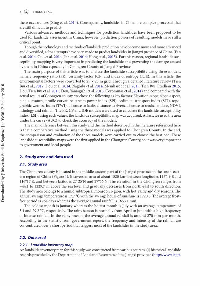
A total of 222 landslides were identified and investigated by field surveys, then, the landslide bound-aries were mapped. This article uses the landslide classification developed by Varnes (1978). Landslide types in the study area include 30 rock falls, 121 rock slides, 69 earth slides and 2 debris flows. The analysis of these landslides shows that the smallest landslide size of the study area is about 2.5 m2 and the largest is 15,000 m2 with an average of about 841.3 m2. In this study, the centroid of these landslides was chosen to map landslide susceptibility. For landslide modelling, these landslides were randomly split into two parts in a 70/30 ratio: Part 1 includes 155 landslides used for model training, whereas the remaining 67 landslides were used for model validation. Figure 1 shows the distribution of these landslide locations in the Chongren County, the Jiangxi province. In this study, the non-landslide points were selected randomly using ArcGIS software, the number of non-landslide points is equal to that of landslide points, and randomly split into two parts (70/30) for verifying models.

2.2.2. Landslide conditioning factorsThe selection of conditioning factors is considered to be a basic step for landslide susceptibility assess-ment. Literature review shows that slope, aspect and lithology are widely used in susceptibility assess-ment, whereas the selection of others factors (i.e. soil type, distance to roads, NVDI) is still debated and dependent on landslide types, characteristic of study areas and method and technique used (Hong et al. 2015; Tien Bui, Tuan et al. 2015; Tien Bui et al., 2014).

The number of conditioning factors to be used for landslide susceptibility assessments is also debated and varies from few factors (Pradhan et al. 2010; Akgun 2012; Tien Bui, Pradhan 2015) to a larger number of factors (Catani et al. 2013; Dou, Tien Bui et al. 2015; Meinhardt et al. 2015). However, a landslide model with many factors does not guarantee a high prediction result (Pradhan & Lee 2010). In some cases, the quality of the resulting models is reduced with the inclusion of noise factors (Tien Bui, Tuan et al. 2015).

Figure 1. landslide location map of the study area.

Dow

nloa

ded

by [

Uni

vers

ita S

tudi

la S

apie

nza]

at 0

3:36

12

Janu

ary

2016

4 H. HONg ET Al.

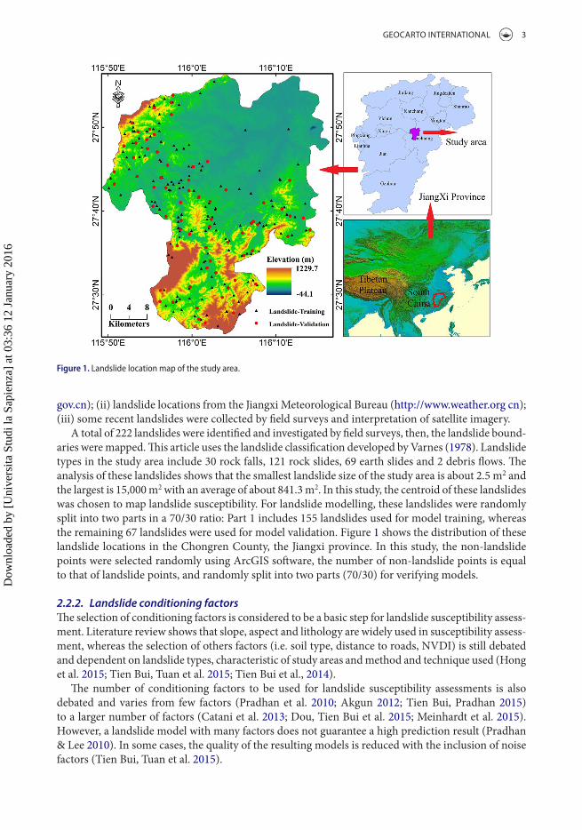
Figure 2. landslide conditioning factors include (a) Slope, (b) aspect, (c) plan curvature, (d) profile curvature, (e) altitude, (f ) distance to rivers, (g) distance to roads, (h) distance to faults, (i) land use, (j) nDVI, (k) stream power index (SPI), (l) sediment transport index, (m) topographic witness index (tWI), (n) lithology, (o) rainfall.

Dow

nloa

ded

by [

Uni

vers

ita S

tudi

la S

apie

nza]

at 0

3:36

12

Janu

ary

2016

gEOCARTO INTERNATIONAl 5

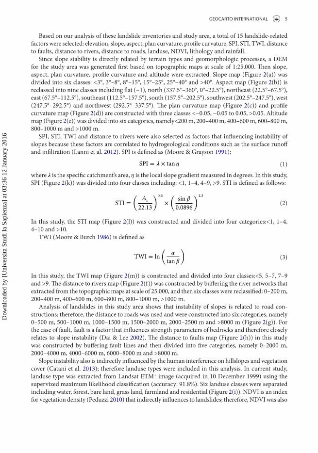
Based on our analysis of these landslide inventories and study area, a total of 15 landslide-related factors were selected: elevation, slope, aspect, plan curvature, profile curvature, SPI, STI, TWI, distance to faults, distance to rivers, distance to roads, landuse, NDVI, lithology and rainfall.

Since slope stability is directly related by terrain types and geomorphologic processes, a DEM for the study area was generated first based on topographic maps at scale of 1:25,000. Then slope, aspect, plan curvature, profile curvature and altitude were extracted. Slope map (Figure 2(a)) was divided into six classes: <3°, 3°–8°, 8°–15°, 15°–25°, 25°–40° and >40°. Aspect map (Figure 2(b)) is reclassed into nine classes including flat (−1), north (337.5°–360°, 0°–22.5°), northeast (22.5°–67.5°), east (67.5°–112.5°), southeast (112.5°–157.5°), south (157.5°–202.5°), southwest (202.5°–247.5°), west (247.5°–292.5°) and northwest (292.5°–337.5°). The plan curvature map (Figure 2(c)) and profile curvature map (Figure 2(d)) are constructed with three classes <−0.05, −0.05 to 0.05, >0.05. Altitude map (Figure 2(e)) was divided into six categories, namely<200 m, 200–400 m, 400–600 m, 600–800 m, 800–1000 m and >1000 m.

SPI, STI, TWI and distance to rivers were also selected as factors that influencing instability of slopes because these factors are correlated to hydrogeological conditions such as the surface runoff and infiltration (Lanni et al. 2012). SPI is defined as (Moore & Grayson 1991):

where � is the specific catchment’s area, η is the local slope gradient measured in degrees. In this study, SPI (Figure 2(k)) was divided into four classes including: <1, 1–4, 4–9, >9. STI is defined as follows:

In this study, the STI map (Figure 2(l)) was constructed and divided into four categories:<1, 1–4, 4–10 and >10.

TWI (Moore & Burch 1986) is defined as

In this study, the TWI map (Figure 2(m)) is constructed and divided into four classes:<5, 5–7, 7–9 and >9. The distance to rivers map (Figure 2(f)) was constructed by buffering the river networks that extracted from the topographic maps at scale of 25.000, and then six classes were reclassified: 0–200 m, 200–400 m, 400–600 m, 600–800 m, 800–1000 m, >1000 m.

Analysis of landslides in this study area shows that instability of slopes is related to road con-structions; therefore, the distance to roads was used and were constructed into six categories, namely 0–500 m, 500–1000 m, 1000–1500 m, 1500–2000 m, 2000–2500 m and >8000 m (Figure 2(g)). For the case of fault, fault is a factor that influences strength parameters of bedrocks and therefore closely relates to slope instability (Dai & Lee 2002). The distance to faults map (Figure 2(h)) in this study was constructed by buffering fault lines and then divided into five categories, namely 0–2000  m, 2000–4000 m, 4000–6000 m, 6000–8000 m and >8000 m.

Slope instability also is indirectly influenced by the human interference on hillslopes and vegetation cover (Catani et al. 2013); therefore landuse types were included in this analysis. In current study, landuse type was extracted from Landsat ETM+ image (acquired in 10 December 1999) using the supervized maximum likelihood classification (accuracy: 91.8%). Six landuse classes were separated including water, forest, bare land, grass land, farmland and residential (Figure 2(i)). NDVI is an index for vegetation density (Peduzzi 2010) that indirectly influences to landslides; therefore, NDVI was also

(1)SPI = � × tan �

(2)STI =

(As

22.13

)0.6

×

(sin �

0.0896

)1.3

(3)TWI = ln

(�

tan �

)

Dow

nloa

ded

by [

Uni

vers

ita S

tudi

la S

apie

nza]

at 0

3:36

12

Janu

ary

2016

6 H. HONg ET Al.

used in this analysis. NDVI values were estimated from the aforementioned Landsat satellite image ETM+ using the common equation as follows:

where NIR is the reflectance of the Earth’s surface in the near infrared channel (0.725–1.1 μm) and VIS is the reflectance in the visible portion of the spectrum or the red channel (0.5–0.68 μm) (Tucker & Sellers 1986). The NDVI map was divided into five classes:<0.10, 0.10–0.20, 0.20–0.30, 0.30–0.40 and >0.40 (Figure 2(j)).

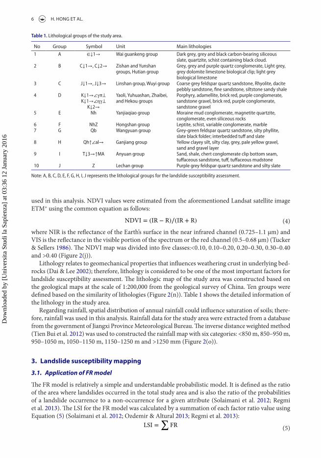
Lithology relates to geomechanical properties that influences weathering crust in underlying bed-rocks (Dai & Lee 2002); therefore, lithology is considered to be one of the most important factors for landslide susceptibility assessment. The lithologic map of the study area was constructed based on the geological maps at the scale of 1:200,000 from the geological survey of China. Ten groups were defined based on the similarity of lithologies (Figure 2(n)). Table 1 shows the detailed information of the lithology in the study area.

Regarding rainfall, spatial distribution of annual rainfall could influence saturation of soils; there-fore, rainfall was used in this analysis. Rainfall data for the study area were extracted from a database from the government of Jiangxi Province Meteorological Bureau. The inverse distance weighted method (Tien Bui et al. 2012) was used to constructed the rainfall map with six categories: <850 m, 850–950 m, 950–1050 m, 1050–1150 m, 1150–1250 m and >1250 mm (Figure 2(o)).

3. Landslide susceptibility mapping

3.1. Application of FR model

The FR model is relatively a simple and understandable probabilistic model. It is defined as the ratio of the area where landslides occurred in the total study area and is also the ratio of the probabilities of a landslide occurrence to a non-occurrence for a given attribute (Solaimani et al. 2012; Regmi et al. 2013). The LSI for the FR model was calculated by a summation of each factor ratio value using Equation (5) (Solaimani et al. 2012; Ozdemir & Altural 2013; Regmi et al. 2013):

(4)NDVI = (IR − R)∕(IR + R)

(5)LSI =∑

FR

Table 1. lithological groups of the study area.

note: a, B, c, D, e, F, G, H, I, J represents the lithological groups for the landslide susceptibility assessment.

No group Symbol Unit Main lithologies1 a ∈↓1→ Wai guankeng group Dark grey, grey and black carbon-bearing siliceous

slate, quartzite, schist containing black cloud.2 B c↓1→, c↓2→ Zishan and Yunshan

groups, Hutian groupGrey, grey and purple quartz conglomerate, light grey, grey dolomite limestone biological clip; light grey biological limestone

3 c J↓1→, J↓3→ linshan group, Wuyi group coarse grey feldspar quartz sandstone, rhyolite, dacite pebbly sandstone, fine sandstone, siltstone sandy shale

4 D K↓1→∠γπ⊥ Yaoli, Yuhuashan, Zhaibei, and Hekou groups

Porphyry, adamellite, brick red, purple conglomerate, sandstone gravel, brick red, purple conglomerate, sandstone gravel

K↓1→∠ηγ⊥K↓2→

5 e nh Yanjiaqiao group Moraine mud conglomerate, magnetite quartzite, conglomerate, even siliceous rocks

6 F nhZ Hongshan group leptite, schist, variable conglomerate, marble7 G Qb Wangyuan group Grey-green feldspar quartz sandstone, silty phyllite,

slate black folder; interbedded tuff and slate8 H Qh↑∠al→ Ganjiang group Yellow clayey silt, silty clay, grey, pale yellow gravel,

sand and gravel layer9 I t↓3→↑Ma anyuan group Sand, shale, chert conglomerate clip bottom seam,

tuffaceous sandstone, tuff, tuffaceous mudstone10 J Z lechan group Purple grey feldspar quartz sandstone and silty slate

Dow

nloa

ded

by [

Uni

vers

ita S

tudi

la S

apie

nza]

at 0

3:36

12

Janu

ary

2016

gEOCARTO INTERNATIONAl 7

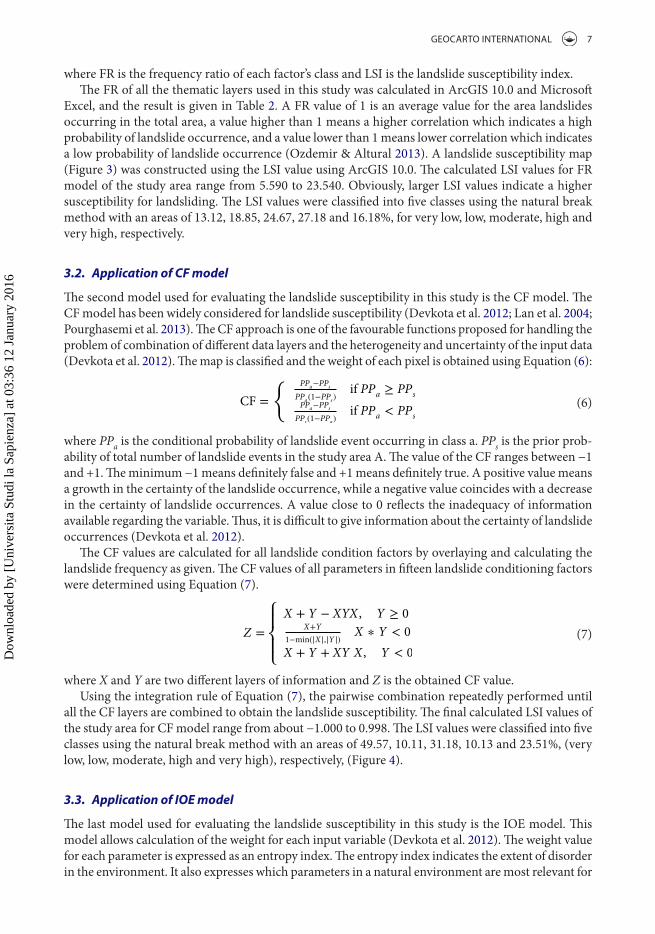
where FR is the frequency ratio of each factor’s class and LSI is the landslide susceptibility index.The FR of all the thematic layers used in this study was calculated in ArcGIS 10.0 and Microsoft

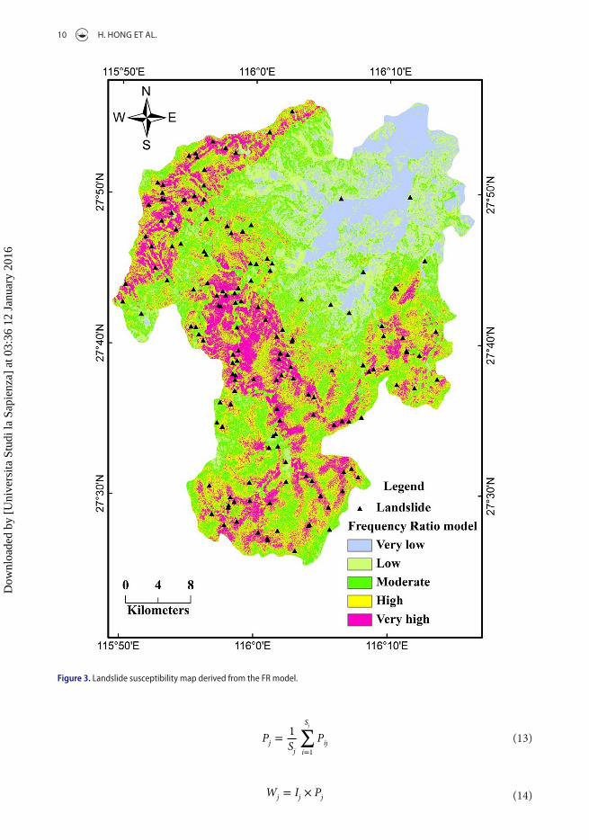
Excel, and the result is given in Table 2. A FR value of 1 is an average value for the area landslides occurring in the total area, a value higher than 1 means a higher correlation which indicates a high probability of landslide occurrence, and a value lower than 1 means lower correlation which indicates a low probability of landslide occurrence (Ozdemir & Altural 2013). A landslide susceptibility map (Figure 3) was constructed using the LSI value using ArcGIS 10.0. The calculated LSI values for FR model of the study area range from 5.590 to 23.540. Obviously, larger LSI values indicate a higher susceptibility for landsliding. The LSI values were classified into five classes using the natural break method with an areas of 13.12, 18.85, 24.67, 27.18 and 16.18%, for very low, low, moderate, high and very high, respectively.

3.2. Application of CF model

The second model used for evaluating the landslide susceptibility in this study is the CF model. The CF model has been widely considered for landslide susceptibility (Devkota et al. 2012; Lan et al. 2004; Pourghasemi et al. 2013). The CF approach is one of the favourable functions proposed for handling the problem of combination of different data layers and the heterogeneity and uncertainty of the input data (Devkota et al. 2012). The map is classified and the weight of each pixel is obtained using Equation (6):

where PPa is the conditional probability of landslide event occurring in class a. PPs is the prior prob-ability of total number of landslide events in the study area A. The value of the CF ranges between −1 and +1. The minimum −1 means definitely false and +1 means definitely true. A positive value means a growth in the certainty of the landslide occurrence, while a negative value coincides with a decrease in the certainty of landslide occurrences. A value close to 0 reflects the inadequacy of information available regarding the variable. Thus, it is difficult to give information about the certainty of landslide occurrences (Devkota et al. 2012).

The CF values are calculated for all landslide condition factors by overlaying and calculating the landslide frequency as given. The CF values of all parameters in fifteen landslide conditioning factors were determined using Equation (7).

where X and Y are two different layers of information and Z is the obtained CF value.Using the integration rule of Equation (7), the pairwise combination repeatedly performed until

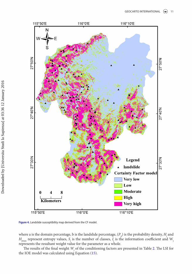
all the CF layers are combined to obtain the landslide susceptibility. The final calculated LSI values of the study area for CF model range from about −1.000 to 0.998. The LSI values were classified into five classes using the natural break method with an areas of 49.57, 10.11, 31.18, 10.13 and 23.51%, (very low, low, moderate, high and very high), respectively, (Figure 4).

3.3. Application of IOE model

The last model used for evaluating the landslide susceptibility in this study is the IOE model. This model allows calculation of the weight for each input variable (Devkota et al. 2012). The weight value for each parameter is expressed as an entropy index. The entropy index indicates the extent of disorder in the environment. It also expresses which parameters in a natural environment are most relevant for

(6)CF =

{ PPa−PPs

PPa(1−PPs)if PPa ≥ PPs

PPa−PPs

PPs(1−PPa)if PPa < PPs

(7)Z =

⎧⎪⎨⎪⎩

X + Y − XYX, Y ≥ 0X+Y

1−min(�X�,�Y �) X ∗ Y < 0

X + Y + XY X , Y < 0Dow

nloa

ded

by [

Uni

vers

ita S

tudi

la S

apie

nza]

at 0

3:36

12

Janu

ary

2016

8 H. HONg ET Al.

Table 2. Spatial relationship between each landslide conditioning factor and landslide by Fr, cF and Ioe models.

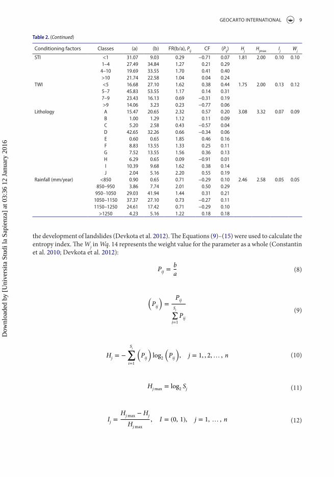
Conditioning factors Classes (a) (b) FR(b/a), Pij CF (Pij) Hj Hjmax Ij Wj

Slope angle (°) <3 31.16 7.10 0.23 −0.77 0.03 2.39 2.58 0.08 0.093–8 24.28 27.74 1.14 0.12 0.17

8–15 17.73 30.97 1.75 0.43 0.2515–25 18.59 28.39 1.53 0.34 0.2225–40 7.82 5.16 0.66 −0.34 0.10

>40 0.42 0.65 1.55 0.36 0.23Slope-aspect Flat 0.70 0.00 0.00 −1.00 0.00 2.99 3.17 0.06 0.05

north 11.34 10.97 0.97 −0.03 0.12northeast 13.04 13.55 1.04 0.04 0.13

east 14.59 13.55 0.93 −0.07 0.12Southeast 12.84 14.19 1.11 0.10 0.14

South 11.02 13.55 1.23 0.19 0.15Southwest 11.76 10.32 0.88 −0.12 0.11

West 12.82 14.19 1.11 0.10 0.14northwest 11.89 9.68 0.81 −0.19 0.10

Plan curvature <−0.05 30.17 25.16 0.83 −0.17 0.29 1.49 1.58 0.06 0.06−0.05 to 0.05 32.22 20.00 0.62 −0.38 0.21

>0.05 37.61 54.84 1.46 0.31 0.50Profile curvature <−0.05 29.94 33.55 1.12 0.11 0.37 1.53 1.58 0.03 0.03

−0.05 to 0.05 33.77 21.29 0.63 −0.37 0.21> 0.05 36.29 45.16 1.24 0.20 0.41

altitude (m) <200 81.66 89.03 1.09 0.08 0.34 1.9 2.58 0.26 0.14200–400 13.43 8.39 0.62 −0.38 0.20400–600 3.15 1.29 0.41 −0.59 0.13600–800 1.21 1.29 1.06 0.06 0.33

800–1000 0.42 0.00 0.00 −1.00 0.00>1000 0.13 0.00 0.00 −1.00 0.00

Distance to rivers (m) 0–200 27.49 49.68 1.81 0.45 0.41 1.96 2.58 0.24 0.18200–400 23.26 34.19 1.47 0.32 0.33400–600 19.28 9.03 0.47 −0.53 0.11600–800 14.43 5.16 0.36 −0.64 0.08

800–1000 9.08 0.00 0.00 −1.00 0.00>1000 6.46 1.94 0.30 −0.70 0.07

Distance to roads (m) 0–500 31.16 50.97 1.64 0.39 0.35 2.34 2.58 0.09 0.07500–1000 25.17 19.35 0.77 −0.23 0.16

1000–1500 19.63 16.13 0.82 −0.18 0.171500–2000 12.21 8.39 0.69 −0.31 0.152000–2500 6.66 4.52 0.68 −0.32 0.14

>2500 5.18 0.65 0.12 −0.88 0.03Distance to faults (m) 0–2000 24.60 30.97 1.26 0.21 0.24 2.2 2.32 0.05 0.05

2000–4000 19.99 25.81 1.29 0.23 0.254000–6000 17.36 23.23 1.34 0.25 0.266000–8000 12.59 11.61 0.92 −0.08 0.18

>8000 25.46 8.39 0.33 −0.67 0.06land use Water 2.35 0.65 0.54 −0.46 0.14 1.76 2.58 0.32 0.20

Forest 28.29 45.81 1.59 0.37 0.42Bare land 0.65 0.00 0.00 −1.00 0.00Grass land 18.17 21.94 1.19 0.16 0.32Farmland 1.31 0.00 0.00 −1.00 0.00

residential 49.23 31.61 0.63 −0.37 0.17nDVI <0.10 35.58 18.06 0.51 −0.49 0.09 2.22 2.32 0.04 0.05

0.10–0.20 22.17 20.65 0.93 −0.07 0.160.20–0.30 20.49 24.52 1.20 0.16 0.210.30–0.40 17.05 30.97 1.82 0.45 0.32

>0.40 4.71 5.81 1.23 0.19 0.22SPI <1 11.94 1.29 0.11 −0.89 0.03 1.71 2.00 0.15 0.12

1–4 22.50 18.06 0.80 −0.20 0.244–9 20.22 24.52 1.21 0.18 0.36>9 45.34 56.13 1.24 0.19 0.37

(continued)

Dow

nloa

ded

by [

Uni

vers

ita S

tudi

la S

apie

nza]

at 0

3:36

12

Janu

ary

2016

gEOCARTO INTERNATIONAl 9

the development of landslides (Devkota et al. 2012). The Equations (9)–(15) were used to calculate the entropy index. The Wj in Wq. 14 represents the weight value for the parameter as a whole (Constantin et al. 2010; Devkota et al. 2012):

(8)Pij =b

a

(9)

�Pij

�=

Pij

Sj∑j=1

Pij

(10)Hj = −

Sj∑i=1

(Pij

)log2

(Pij

), j = 1, , 2,… , n

(11)Hjmax = log2 Sj

(12)Ij =Hjmax −Hj

Hjmax

, I = (0, 1), j = 1, … , n

Conditioning factors Classes (a) (b) FR(b/a), Pij CF (Pij) Hj Hjmax Ij Wj

StI <1 31.07 9.03 0.29 −0.71 0.07 1.81 2.00 0.10 0.101–4 27.49 34.84 1.27 0.21 0.29

4–10 19.69 33.55 1.70 0.41 0.40>10 21.74 22.58 1.04 0.04 0.24

tWI <5 16.68 27.10 1.62 0.38 0.44 1.75 2.00 0.13 0.125–7 45.83 53.55 1.17 0.14 0.317–9 23.43 16.13 0.69 −0.31 0.19>9 14.06 3.23 0.23 −0.77 0.06

lithology a 15.47 20.65 2.32 0.57 0.20 3.08 3.32 0.07 0.09B 1.00 1.29 1.12 0.11 0.09c 5.20 2.58 0.43 −0.57 0.04D 42.65 32.26 0.66 −0.34 0.06e 0.60 0.65 1.85 0.46 0.16F 8.83 13.55 1.33 0.25 0.11G 7.52 13.55 1.56 0.36 0.13H 6.29 0.65 0.09 −0.91 0.01I 10.39 9.68 1.62 0.38 0.14J 2.04 5.16 2.20 0.55 0.19

rainfall (mm/year) <850 0.90 0.65 0.71 −0.29 0.10 2.46 2.58 0.05 0.05850–950 3.86 7.74 2.01 0.50 0.29

950–1050 29.03 41.94 1.44 0.31 0.211050–1150 37.37 27.10 0.73 −0.27 0.111150–1250 24.61 17.42 0.71 −0.29 0.10

>1250 4.23 5.16 1.22 0.18 0.18

Table 2. (Continued)

Dow

nloa

ded

by [

Uni

vers

ita S

tudi

la S

apie

nza]

at 0

3:36

12

Janu

ary

2016

10 H. HONg ET Al.

(13)Pj =1

Sj

Sj∑i=1

Pij

(14)Wj = Ij × Pj

Figure 3. landslide susceptibility map derived from the Fr model.

Dow

nloa

ded

by [

Uni

vers

ita S

tudi

la S

apie

nza]

at 0

3:36

12

Janu

ary

2016

gEOCARTO INTERNATIONAl 11

where a is the domain percentage, b is the landslide percentage, (Pij) is the probability density, Hj and Hjmax represent entropy values, Sj is the number of classes, Ij is the information coefficient and Wj represents the resultant weight value for the parameter as a whole.

The results of the final weight Wj of the conditioning factors are presented in Table 2. The LSI for the IOE model was calculated using Equation (15).

Figure 4. landslide susceptibility map derived from the cF model.

Dow

nloa

ded

by [

Uni

vers

ita S

tudi

la S

apie

nza]

at 0

3:36

12

Janu

ary

2016

12 H. HONg ET Al.

(15)

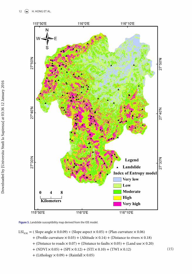
LSIIOE = ( Slope angle × 0.0.09) + (Slope aspect × 0.05) + (Plan curvature × 0.06)

+ (Profile curvature × 0.03) + (Altitude × 0.14) + (Distance to rivers × 0.18)

+ (Distance to roads × 0.07) + (Distance to faults × 0.05) + (Land use × 0.20)

+ (NDVI × 0.05) + (SPI × 0.12) + (STI × 0.10) + (TWI × 0.12)

+ (Lithology × 0.09) + (Rainfall × 0.05) (1)

Figure 5. landslide susceptibility map derived from the Ioe model.

Dow

nloa

ded

by [

Uni

vers

ita S

tudi

la S

apie

nza]

at 0

3:36

12

Janu

ary

2016

gEOCARTO INTERNATIONAl 13

The calculated LSI values for IOE model of the study area range from 0.446 to 2.199. The LSI map was classified into 5 landslide susceptibility classes based on natural break method with an area of 11.89, 22.33, 25.95, 24.74 and 15.09%, for very low, low, moderate, high and very high classes, respectively (Figure 5).

4. Validation and comparison

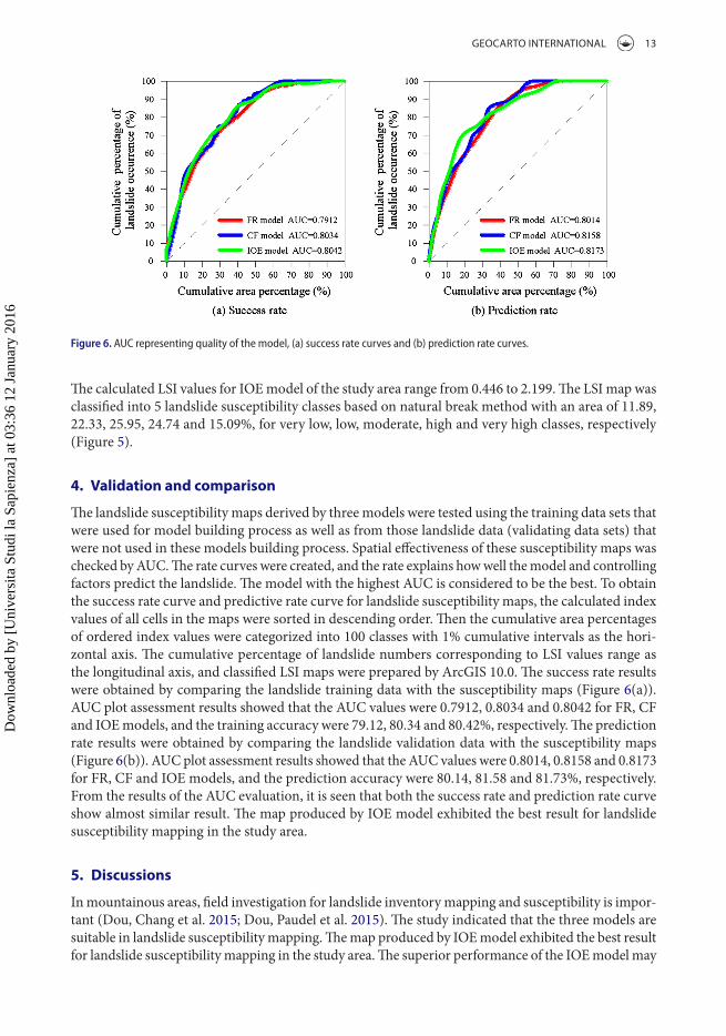
The landslide susceptibility maps derived by three models were tested using the training data sets that were used for model building process as well as from those landslide data (validating data sets) that were not used in these models building process. Spatial effectiveness of these susceptibility maps was checked by AUC. The rate curves were created, and the rate explains how well the model and controlling factors predict the landslide. The model with the highest AUC is considered to be the best. To obtain the success rate curve and predictive rate curve for landslide susceptibility maps, the calculated index values of all cells in the maps were sorted in descending order. Then the cumulative area percentages of ordered index values were categorized into 100 classes with 1% cumulative intervals as the hori-zontal axis. The cumulative percentage of landslide numbers corresponding to LSI values range as the longitudinal axis, and classified LSI maps were prepared by ArcGIS 10.0. The success rate results were obtained by comparing the landslide training data with the susceptibility maps (Figure 6(a)). AUC plot assessment results showed that the AUC values were 0.7912, 0.8034 and 0.8042 for FR, CF and IOE models, and the training accuracy were 79.12, 80.34 and 80.42%, respectively. The prediction rate results were obtained by comparing the landslide validation data with the susceptibility maps (Figure 6(b)). AUC plot assessment results showed that the AUC values were 0.8014, 0.8158 and 0.8173 for FR, CF and IOE models, and the prediction accuracy were 80.14, 81.58 and 81.73%, respectively. From the results of the AUC evaluation, it is seen that both the success rate and prediction rate curve show almost similar result. The map produced by IOE model exhibited the best result for landslide susceptibility mapping in the study area.

5. Discussions

In mountainous areas, field investigation for landslide inventory mapping and susceptibility is impor-tant (Dou, Chang et al. 2015; Dou, Paudel et al. 2015). The study indicated that the three models are suitable in landslide susceptibility mapping. The map produced by IOE model exhibited the best result for landslide susceptibility mapping in the study area. The superior performance of the IOE model may

Figure 6. aUc representing quality of the model, (a) success rate curves and (b) prediction rate curves.

Dow

nloa

ded

by [

Uni

vers

ita S

tudi

la S

apie

nza]

at 0

3:36

12

Janu

ary

2016

14 H. HONg ET Al.

be due to the fact that IOE model does not need any assumptions about the distribution of variables, nor assume a linear model, and it can select the most conditioning factors on landslide occurrence through this model (Pourghasemi et al. 2013). The results of current study showed that landuse, dis-tance to rivers and rainfall were the most three important factors with weigh values of 0.20, 0.18 and 0.14, respectively. Moreover, the results also showed that profile curvature, slope-aspect and distance to faults had the lowest importance in landslide occurrence of the study area.

6. Conclusions

Landslide susceptibility maps provide fundamental and essential information of the causes and effective factors on landslide occurrence. These maps can be effective in hazard management and its mitigation measures (Tien Bui et al. 2013; Pourghasemi et al. 2013). In the current study, three statistical models named FR, CF and IOE were used for landslide susceptibility mapping. Their performances were com-pared to determine the most suitable model for landslide susceptibility. In this process, a total of 222 landslides were identified and mapped by field investigations and interpretation of satellite imagery. The models were built using 70% of the landslides data and validated using the remaining 30% of the landslides data. In the study, fifteen landslide-related factors were used including elevation, slope, slope-aspect, plan curvature, profile curvature, SPI, STI, TWI, distance to faults, distance to rivers, distance to roads, landuse, NDVI, lithology and rainfall. The three landslide susceptibility maps were classified into five classes, i.e. very low, low, moderate, high and very high according to the natural break method. The AUC plots showed that the training accuracy were 79.12, 80.34 and 80.42%, and the prediction accuracy were 80.14, 81.58 and 81.73%, for FR, CF and IOE models, respectively. As a final conclusion, these landslide susceptibility maps produced in this study can be used for optimum management by decision makers and landuse planners, and also avoidance of landslide susceptible regions in study area. Also, it is worth mentioning that the similar method can be used elsewhere where the same geological and topographical feature prevails.

Disclosure statementThe authors declare no conflict of interest.

FundingThis research was supported by the National Natural Science Foundation of China [grant numbers 41472202, 41202235].

ORCIDDieu Tien Bui   http://orcid.org/0000-0001-5161-6479

ReferencesAkgun A. 2012. A comparison of landslide susceptibility maps produced by logistic regression, multi-criteria decision,

and likelihood ratio methods: a case study at İzmir, Turkey. Landslides. 9:93–106. doi:10.1007/s10346-011-0283-7.Catani F, Lagomarsino D, Segoni S, Tofani V. 2013. Landslide susceptibility estimation by random forests technique:

sensitivity and scaling issues. Nat Hazards Earth Syst Sci. 13:2815–2831. doi:10.5194/nhess-13-2815-2013.Constantin M, Bednarik M, Jurchescu MC, Vlaicu M. 2010. Landslide susceptibility assessment using the bivariate

statistical analysis and the index of entropy in the Sibiciu Basin (Romania). Environ Earth Sci. 63:397–406. doi:10.1007/s12665-010-0724-y.

Corominas J, van Westen C, Frattini P, Cascini L, Malet JP, Fotopoulou S, Catani F, Van Den Eeckhaut M, Mavrouli O, Agliardi F, Pitilakis K, Winter MG, Pastor M, Ferlisi S, Tofani V, Hervás J, Smith JT. 2014. Recommendations for the quantitative analysis of landslide risk. Bulletin of Engineering Geology and the Environment. 73:209–263.

Dai FC, Lee CF. 2002. Landslide characteristics and slope instability modeling using GIS, Lantau Island, Hong Kong. Geomorphology. 42:213–228.

Dow

nloa

ded

by [

Uni

vers

ita S

tudi

la S

apie

nza]

at 0

3:36

12

Janu

ary

2016

gEOCARTO INTERNATIONAl 15

Devkota KC, Regmi A, Pourghasemi H, Yoshida K, Pradhan B, Ryu I, Dhital M, Althuwaynee O. 2012. Landslide susceptibility mapping using certainty factor, index of entropy and logistic regression models in GIS and their comparison at Mugling-Narayanghat road section in Nepal Himalaya. Nat Hazards. 65:135–165. doi:10.1007/s11069-012-0347-6.

Dou J, Tien Bui D, Yunus AP, Jia K, Song X, Revhaug I, Xia H, Zhu Z. 2015. Optimization of causative factors for landslide susceptibility evaluation using remote sensing and GIS Data in parts of Niigata, Japan. PLOS ONE. 10:e0133262. doi:10.1371/journal.pone.0133262.

Dou J, Chang K-T, Chen S, Yunus AP, Liu J-K, Xia H, Zhu Z. 2015. Automatic case-based reasoning approach for landslide detection: integration of object-oriented image analysis and a genetic algorithm. Remote Sens. 7:4318–4342.

Dou J, Oguchi T, Hayakawa YS, Uchiyama S, Saito H, Paudel U. 2014. GIS-based landslide susceptibility mapping using a certainty factor model and its validation in the Chuetsu Area, Central Japan. In: Landslide science for a safer geoenvironment. Springer International; p. 419–424.

Dou J, Paudel U, Oguchi T, Uchiyama S, Hayakavva YS. 2015. Shallow and deep-seated landslide differentiation using support vector machines: a case study of the Chuetsu Area, Japan. Terr Atmos Oceanic Sci. 26.

Dou J, Yamagishi H, Pourghasemi HR, Yunus AP, Song X, Xu Y, Zhu Z. 2015. An integrated artificial neural network model for the landslide susceptibility assessment of Osado Island, Japan. Nat Hazards. 78:1749–1776.

Fan XM, Rossiter DG, van Westen CJ, Xu Q, Görüm T. 2014. Empirical prediction of coseismic landslide dam formation. Earth Surf Process Landforms. 39:1913–1926. doi:10.1002/esp.3585.

Guo XH, Lai ZP, Sun Z, Li XL, Yang TB. 2014. Luminescence dating of Suozi landslide in the Upper Yellow River of the Qinghai-Tibetan Plateau, China. Quat Int. 349:159–166. doi:10.1016/j.quaint.2014.03.014.

Hong H, Pradhan B, Xu C, Tien Bui D. 2015. Spatial prediction of landslide hazard at the Yihuang area (China) using two-class kernel logistic regression, alternating decision tree and support vector machines. Catena. 133:266–281. doi:10.1016/j.catena.2015.05.019.

Hong H, Xu C, Revhaug I, Tien Bui D. 2015. Spatial Prediction of Landslide Hazard at the Yihuang Area (China): A Comparative Study on the Predictive Ability of Backpropagation Multi-layer Perceptron Neural Networks and Radial Basic Function Neural Networks. In: Robbi Sluter C, Madureira Cruz CB, Leal de Menezes PM, editors. Cartography - Maps Connecting the World. Springer International Publishing; p. 175–188.

Jian WX, Xu Q, Yang HF, Wang FW. 2014. Mechanism and failure process of Qianjiangping landslide in the three Gorges Reservoir, China. Environ Earth Sci. 72:2999–3013. doi:10.1007/s12665-014-3205-x.

Kwan JSH, Chan SL, Cheuk JCY, Koo RCH. 2014. A case study on an open hillside landslide impacting on a flexible rockfall barrier at Jordan Valley, Hong Kong. Landslides. 11:1037–1050. doi:10.1007/s10346-013-0461-x.

Lan HX, Zhou CH, Wang LJ, Zhang HY, Li RH. 2004. Landslide hazard spatial analysis and prediction using GIS in the Xiaojiang watershed, Yunnan, China. Eng Geol. 76:109–128. doi:10.1016/j.enggeo.2004.06.009.

Lanni C, Borga M, Rigon R, Tarolli P. 2012. Modelling shallow landslide susceptibility by means of a subsurface flow path connectivity index and estimates of soil depth spatial distribution. Hydrol Earth Syst Sci. 16:3959–3971.

Li Y, Zhou R, Zhao G, Li H, Su D, Ding H, Yan Z, Yan L, Yun K, Ma C. 2014. Tectonic uplift and landslides triggered by the Wenchuan earthquake and constraints on orogenic growth: a case study from Hongchun Gully, Longmen Mountains, Sichuan, China. Quat Int. 349:142–152. doi:10.1016/j.quaint.2014.05.005.

Meinhardt M, Fink M, Tünschel H. 2015. Landslide susceptibility analysis in central Vietnam based on an incomplete landslide inventory: comparison of a new method to calculate weighting factors by means of bivariate statistics. Geomorphology. 234:80–97. doi:10.1016/j.geomorph.2014.12.042.

Moore ID, Burch GJ. 1986. Sediment transport capacity of sheet and rill flow: application of unit stream power theory. Water Resour Res. 22:1350–1360.

Moore ID, Grayson RB. 1991. Terrain-based catchment partitioning and runoff prediction using vector elevation data. Water Resour Res. 27:1177–1191.

Naghibi SA, Pourghasemi HR, Pourtaghi ZS, Rezaei A. 2014. Groundwater qanat potential mapping using frequency ratio and Shannon’s entropy models in the Moghan watershed, Iran. Earth Sci Inf. 8:171–186.

Ozdemir A, Altural T. 2013. A comparative study of frequency ratio, weights of evidence and logistic regression methods for landslide susceptibility mapping: Sultan Mountains, SW Turkey. J Asian Earth Sci. 64:180–197. doi:10.1016/j.jseaes.2012.12.014.

Peduzzi P. 2010. Landslides and vegetation cover in the 2005 North Pakistan earthquake: a GIS and statistical quantitative approach. Nat Hazards Earth Syst Sci 10:623–640.

Pourghasemi HR, Moradi HR, Fatemi Aghda SM. 2013. Landslide susceptibility mapping by binary logistic regression, analytical hierarchy process, and statistical index models and assessment of their performances. Nat Hazards. 69:749–779. doi:10.1007/s11069-013-0728-5.

Pourghasemi HR, Pradhan B, Gokceoglu C, Mohammadi M, Moradi HR. 2012. Application of weights-of-evidence and certainty factor models and their comparison in landslide susceptibility mapping at Haraz watershed, Iran. Arab J Geosci. 6:2351–2365. doi:10.1007/s12517-012-0532-7.

Pradhan B, Lee S. 2010. Landslide susceptibility assessment and factor effect analysis: backpropagation artificial neural networks and their comparison with frequency ratio and bivariate logistic regression modelling. Environ Model Softw. 25:747–759. doi:10.1016/j.envsoft.2009.10.016.

Dow

nloa

ded

by [

Uni

vers

ita S

tudi

la S

apie

nza]

at 0

3:36

12

Janu

ary

2016

16 H. HONg ET Al.

Pradhan B, Sezer EA, Gokceoglu C, Buchroithner MF. 2010. Landslide susceptibility mapping by neuro-fuzzy approach in a landslide-prone area (Cameron Highlands, Malaysia). IEEE Trans Geosci Remote Sens. 48:4164–4177. doi:10.1109/tgrs.2010.2050328.

Regmi AD, Devkota KC, Yoshida K, Pradhan B, Pourghasemi HR, Kumamoto T, Akgun A. 2013. Application of frequency ratio, statistical index, and weights-of-evidence models and their comparison in landslide susceptibility mapping in Central Nepal Himalaya. Arab J Geosci. 7:725–742. doi:10.1007/s12517-012-0807-z.

Solaimani K, Mousavi SZ, Kavian A. 2012. Landslide susceptibility mapping based on frequency ratio and logistic regression models. Arab J Geosci. 6:2557–2569. doi:10.1007/s12517-012-0526-5.

Tien Bui D, Pradhan B, Lofman O, Revhaug I, Dick OB. 2012. Landslide susceptibility assessment in the Hoa Binh province of Vietnam: a comparison of the Levenberg-Marquardt and Bayesian regularized neural networks. Geomorphology. 171–172:12–29.

Tien Bui D, Pradhan B, Lofman O, Revhaug I, Dick OB. 2012. Application of support vector machines in landslide susceptibility assessment for the Hoa Binh province (Vietnam) with kernel functions analysis. In: Seppelt R, Voinov AA, Lange S, Bankamp D, editors. Proceedings of the iEMSs Sixth Biennial Meeting: International Congress on Environmental Modelling and Software (iEMSs 2012). International Environmental Modelling and Software Society, Leipzig, Germany, July 2012.

Tien Bui D, Pradhan B, Lofman O, Revhaug I, Dick O. 2013. Regional prediction of landslide hazard using probability analysis of intense rainfall in the Hoa Binh province. Vietnam. Natural Hazards. 66:707–730.

Tien Bui D, Pradhan B, Revhaug I, Trung Tran C. 2014. A Comparative Assessment Between the Application of Fuzzy Unordered Rules Induction Algorithm and J48 Decision Tree Models in Spatial Prediction of Shallow Landslides at Lang Son City, Vietnam. In: Srivastava PK, Mukherjee S, Gupta M, Islam T, editors. Remote Sensing Applications in Environmental Research. Springer International Publishing; p. 87–111.

Tien Bui D, Pradhan B, Revhaug I, Nguyen DB, Pham HV, Bui QN. 2015. A novel hybrid evidential belief function-based fuzzy logic model in spatial prediction of rainfall-induced shallow landslides in the Lang Son city area (Vietnam) Geomatics. Nat Hazards Risk. 6:243–271. doi:10.1080/19475705.2013.843206.

Tien Bui D, Tuan TA, Klempe H, Pradhan B, Revhaug I. 2015. Spatial prediction models for shallow landslide hazards: a comparative assessment of the efficacy of support vector machines, artificial neural networks, kernel logistic regression, and logistic model tree. Landslides. doi:10.1007/s10346-015-0557-6.

Tucker CJ, Sellers PJ. 1986. Satellite remote sensing of primary production. Int J Remote Sens. 7:1395–1416.Varnes DJ. 1978. Slope movement types and processes. Transportation Research Board Special Report, Washington

DC (USA), 176.Xing AG, et al. 2014. Dynamic analysis and field investigation of a fluidized landslide in Guanling, Guizhou, China.

Eng Geol. 181:1–14. doi:10.1016/j.enggeo.2014.07.022.

Dow

nloa

ded

by [

Uni

vers

ita S

tudi

la S

apie

nza]

at 0

3:36

12

Janu

ary

2016