Rajkumar VenkatesanMarketing Analytics Regression

Rajkumar VenkatesanMarketing Analytics

Regression

Rajkumar Venkatesan

Conservatism in Major League BB

• Batting Average = Hits/(Opportunities– Walks)• OnBase% = (Hits+Walks)/Opportunities• OVERUSED: “small ball”

– Sacrifice Bunt• Give up an out to advance the runner

– Stealing Bases• Risk an Out to advance the runner.

• UNDERUSED– Don’t risk making outs and runs

will take care of themselves.


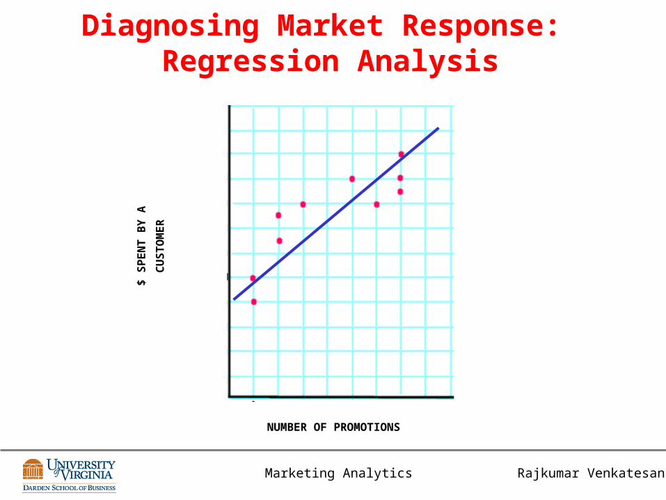
Diagnosing Market Response: Regression Analysis

NUMBER OF PROMOTIONS

$ S

PE

NT

BY

A

CU

ST

OM

ER


Example: Shopper Card Program

Units purchased = a+b1*price paid + b2*feature ad + b3*display

Customer Units Purchased Price Paid Feature Ad Display1 2 1.99 0 01 1 1.99 1 11 2 1.99 1 02 1 2.29 0 02 1 2.29 0 12 5 1 1 02 1 2.29 0 02 1 2.29 1 12 2 2.1 1 13 2 1.99 1 13 2 2.1 1 03 3 1 1 03 1 1.99 0 0

CODE: 1 = YES 1 = YES0 = NO 0 = NO

Data


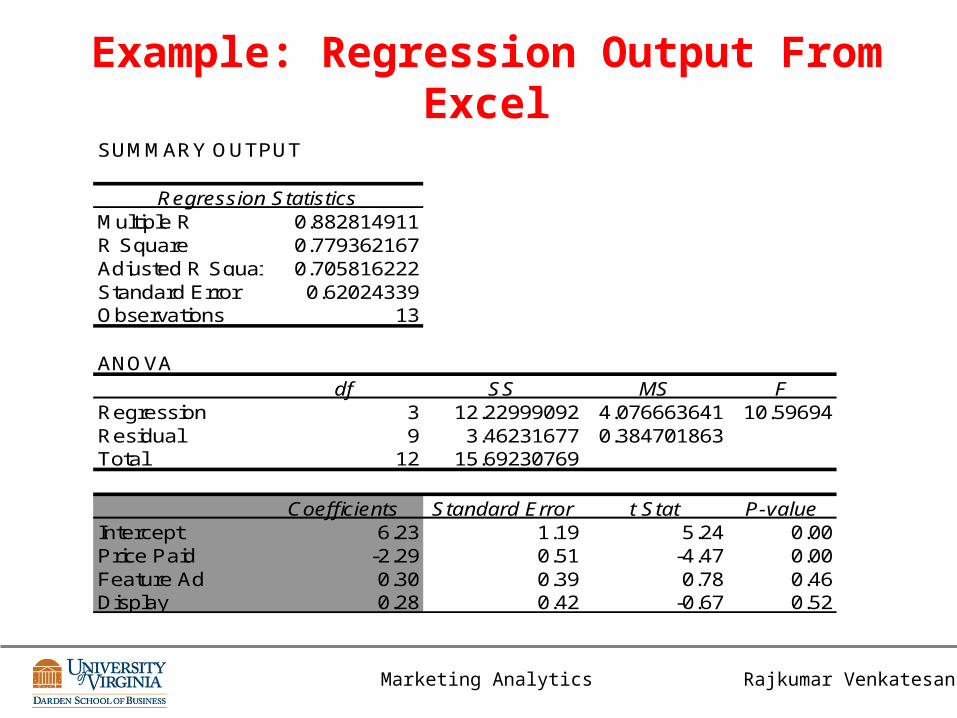
Example: Regression Output From Excel

SUMMARY OUTPUT

Regression StatisticsMultiple R 0.882814911R Square 0.779362167Adjusted R Square 0.705816222Standard Error 0.62024339Observations 13

ANOVAdf SS MS F

Regression 3 12.22999092 4.076663641 10.59694Residual 9 3.46231677 0.384701863Total 12 15.69230769

Coefficients Standard Error t Stat P-valueIntercept 6.23 1.19 5.24 0.00Price Paid -2.29 0.51 -4.47 0.00Feature Ad 0.30 0.39 0.78 0.46Display 0.28 0.42 -0.67 0.52

Rajkumar Venkatesan

Price Elasticity

Marketing Analytics

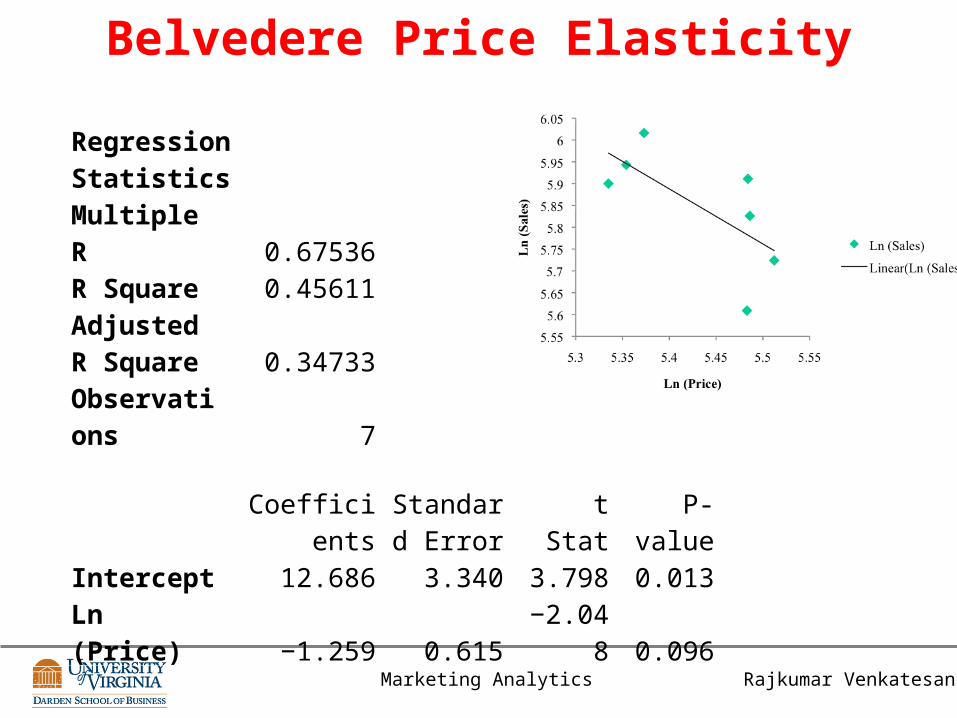
Price elasticity can be derived as the ratio of change in quantity demanded (%∆Q) and percentage change in price (%∆P).

PED = [Change in Sales/Change in Price] × [Price/Sales] = (∆Q/∆P) × (P/Q)

Rajkumar Venkatesan

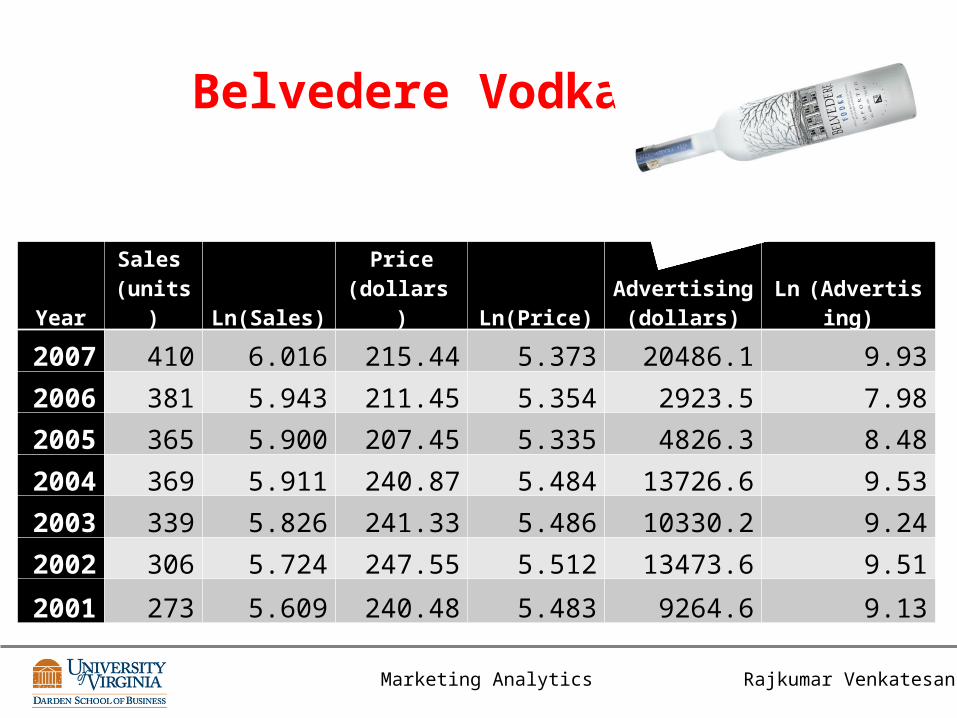
Belvedere Vodka

YearSales (units) Ln(Sales)

Price(dollars ) Ln(Price)

Advertising(dollars) Ln (Advertising)

2007 410 6.016 215.44 5.373 20486.1 9.93

2006 381 5.943 211.45 5.354 2923.5 7.98

2005 365 5.900 207.45 5.335 4826.3 8.48

2004 369 5.911 240.87 5.484 13726.6 9.53

2003 339 5.826 241.33 5.486 10330.2 9.24

2002 306 5.724 247.55 5.512 13473.6 9.51

2001 273 5.609 240.48 5.483 9264.6 9.13

Marketing Analytics

Rajkumar Venkatesan

Belvedere Price Elasticity

Regression StatisticsMultiple R 0.67536R Square 0.45611Adjusted R Square 0.34733Observations 7

CoefficientsStandard

Error t Stat P-valueIntercept 12.686 3.340 3.798 0.013Ln (Price) −1.259 0.615 −2.048 0.096

Marketing Analytics

Rajkumar Venkatesan

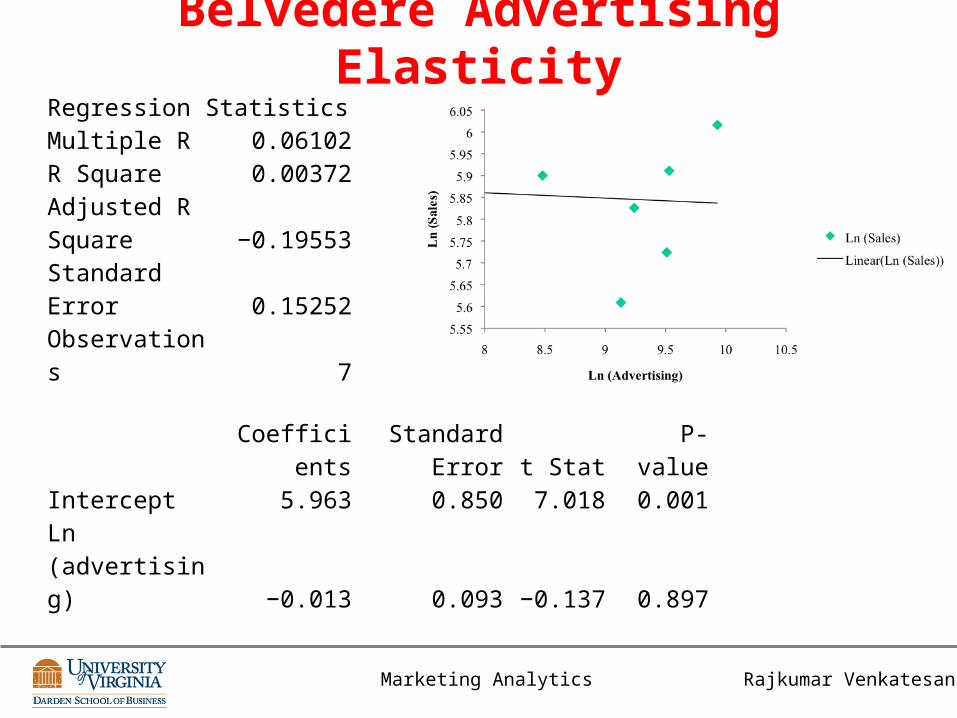
Belvedere Advertising ElasticityRegression StatisticsMultiple R 0.06102R Square 0.00372Adjusted R Square −0.19553Standard Error 0.15252Observations 7

CoefficientsStandard

Error t Stat P-valueIntercept 5.963 0.850 7.018 0.001Ln (advertising) −0.013 0.093 −0.137 0.897

Marketing Analytics



Customer Retention: Logistic Regression

• Linear regression assumes the dependent variable (DV) to be continuous (and normally distributed)

• Often we have variables where there are only 2 different values

• Buy (1) vs no buy (0)• Retain (1) vs lose customer (0)

0- +

Profits


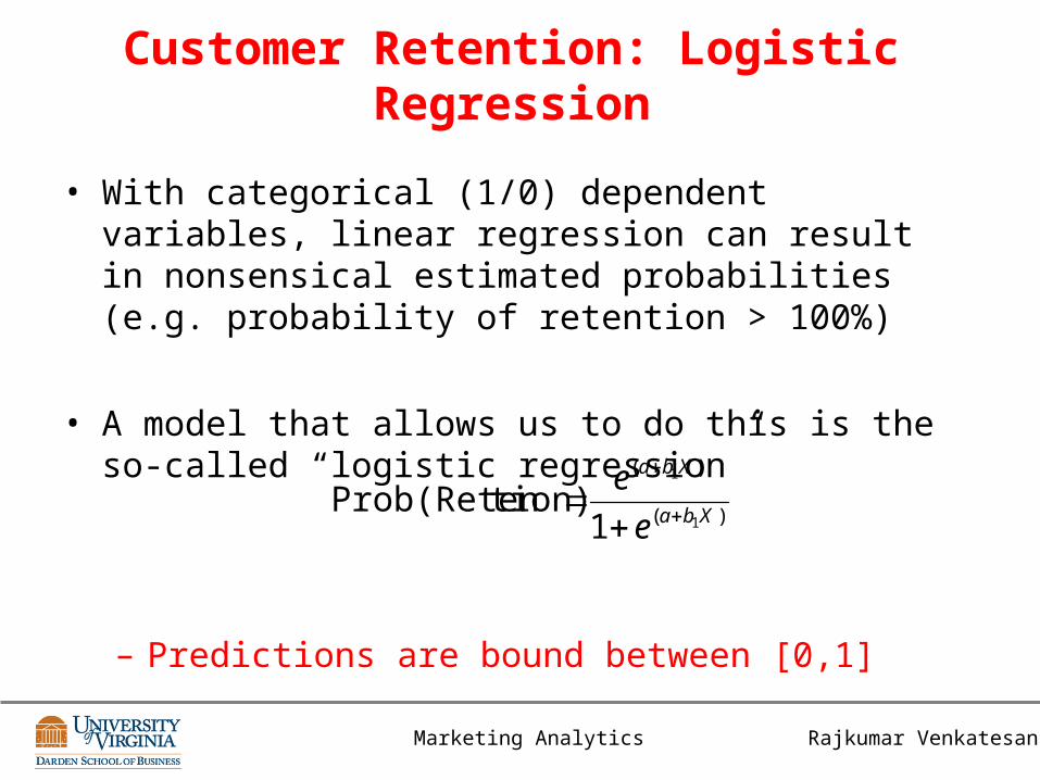
Customer Retention: Logistic Regression

• With categorical (1/0) dependent variables, linear regression can result in nonsensical estimated probabilities (e.g. probability of retention > 100%)

• A model that allows us to do this is the so-called “logistic regression”

– Predictions are bound between [0,1]

)(

)(

1

1

1tion)Prob(Reten Xba

Xba

e

e


0

0.2

0.4

0.6

0.8

1

1.2

-6 -4 -2 0 2 4 6

x

Logistic Prob(retention)


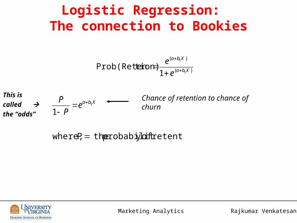
Logistic Regression: The connection to Bookies

)(

)(

1

1

1tion)Prob(Reten Xba

Xba

e

e

retention ofy probabilit theP where,

11

XbaeP

PThis is

called the “odds”

Chance of retention to chance of churn

Rajkumar Venkatesan

SuperBowl 2012 Odds

Green Bay Packers 3.45 to 1

New England Patriots 4.4 to 1

New Orleans Saints 8.5 to 1

Baltimore Ravens 9.5 to 1

San Deigo Chargers 10.5 to 1

Detroit Lions 13 to 1

Houston Texans 17.5 to 1

Pittsburg Steelers 20 to 1

Marketing Analytics


What is Odds?• If you chose a random day of the week (7 days), then the odds that you would

choose a Sunday would be:– (1/7)/[1-(1/7)] = 1/6, but not 1/7.

• The odds against you choosing Sunday are 6/1 = 6 , meaning that it's 6 times more likely that you don't choose Sunday.

• Generally, 'odds' are not quoted to the general public in this format because of the natural confusion with the chance of an event occurring being expressed fractionally as a probability.

• A bookmaker may (for his own purposes) use 'odds' of 'one-sixth', the overwhelming everyday use by most people is odds of the form 6 to 1, 6-1, or 6/1 (all read as 'six-to-one') where the first figure represents the number of ways of failing to achieve the outcome and the second figure is the number of ways of achieving a favorable outcome: thus these are "odds against".

• An event with m to n "odds against" would have probability n/(m + n), while an event with m to n "odds on" would have probability m/(m + n).

Source: http://en.wikipedia.org/wiki/Odds


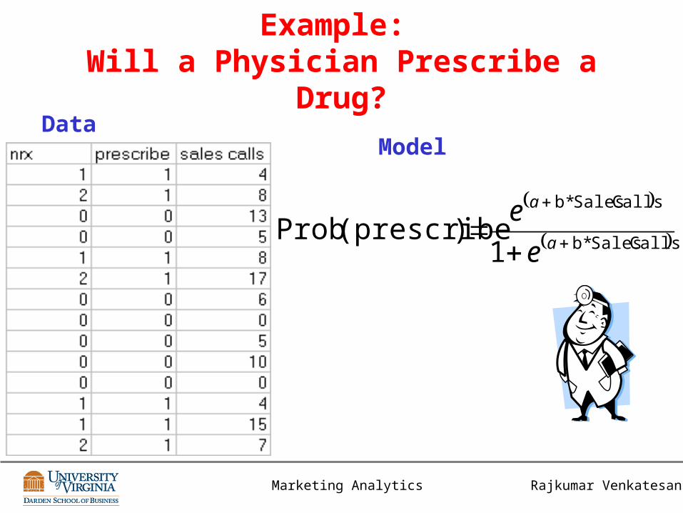
Example: Will a Physician Prescribe a Drug?

Calls Sales b*

Calls Sales b*

1 )(prescribe Prob

a

a

e

e

DataModel


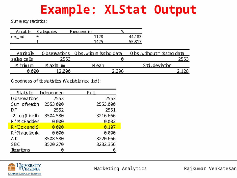
Example: XLStat Output

Goodness of fit statistics (Variable nrx_ind):

Statistic Independent FullObservations 2553 2553Sum of weights 2553.000 2553.000DF 2552 2551-2 Log(Likelihood)3504.580 3216.666R²(McFadden) 0.000 0.082R²(Cox and Snell) 0.000 0.107R²(Nagelkerke) 0.000 0.000AIC 3508.580 3220.666SBC 3520.270 3232.356Iterations 0 6

Summary statistics:

Variable Categories Frequencies %nrx_ind 0 1128 44.183

1 1425 55.817

Variable Observations Obs. with missing data Obs. without missing datasales calls 2553 0 2553

Minimum Maximum Mean Std. deviation0.000 12.000 2.396 2.128


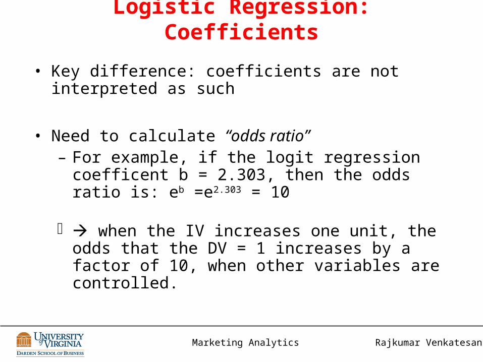
Logistic Regression: Coefficients

• Key difference: coefficients are not interpreted as such

• Need to calculate “odds ratio”– For example, if the logit regression coefficent b = 2.303,

then the odds ratio is: eb =e2.303 = 10

when the IV increases one unit, the odds that the DV = 1 increases by a factor of 10, when other variables are controlled.


Example: XLStat Output

What is the Odds Ratio for Sales Calls?

–Caution: odds ratios that are close to one, do NOT suggest that the coefficients are insignificant – it just means there is 50/50 chance of outcome

Source Value Standard error Wald Chi-Square Pr > Chi²Intercept -0.575 0.064 79.883 < 0.0001sales calls 0.361 0.023 235.781 < 0.0001


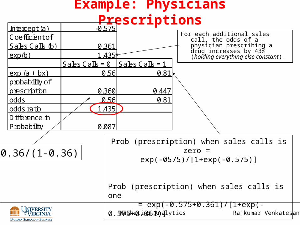
Example: Physicians Prescriptions

For each additional sales call, the odds of a physician prescribing a drug increases by 43% (holding everything else constant).

Prob (prescription) when sales calls is zero = exp(-0575)/[1+exp(-0.575)]

Prob (prescription) when sales calls is one = exp(-0.575+0.361)/[1+exp(-0.575+0.361)]

0.36/(1-0.36)

Intercept (a) -0.575Coefficient of Sales Calls (b) 0.361exp(b) 1.435

Sales Calls = 0 Sales Calls = 1exp (a + bx) 0.56 0.81probability of prescription 0.360 0.447odds 0.56 0.81odds ratio 1.435Difference in Probability 0.087

Rajkumar Venkatesan

Reaction to econometric analysis?


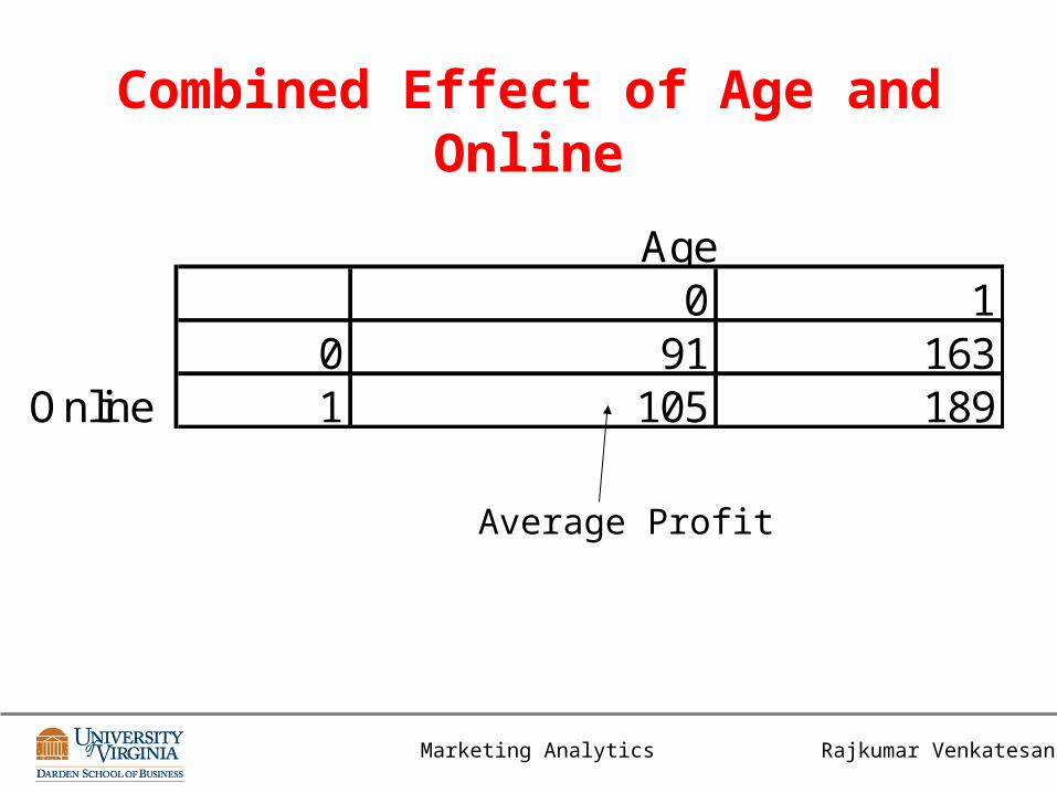
Combined Effect of Age and Online

0 10 91 1631 105 189

Age

Online

Average Profit


Diagnosing Customer Profits and Retention: Common Drivers

Behavioral characteristics• purchase volume/quantity• Frequency of buying • length of relationship• number of product categories purchased• selling costs• customer satisfaction

Demographic/firmographic characteristics• Age, income, gender• Loyalty program membership• Firm size

Psychographic characteristics• Attitudes, values• Interests• Activities

Goal:

To identify

key lever(s)

that “drive”

customer value

Rajkumar Venkatesan

Model Building

• Determine properties of dependent variable– Linear, + ve values, Dummy Variable

• Select model that reflects dependent variable properties– Logistic regression for dummy variables

Marketing Analytics

Rajkumar Venkatesan

Model Building

• Include the decision variable of interest among the independent variable set– Price, advertising, online

• Include common control variables– Quality, Distribution, Demographics, Tenure,

Competition etc.

Marketing Analytics

Rajkumar Venkatesan

Model Building

• Does including lagged dependent variable lead to UNIT ROOT?

• If UNIT ROOT, use difference as the dependent variable

• Are some independent variables correlated more than 0.8. If so, can we eliminate one of the correlated variables or combine them.

Marketing Analytics

Rajkumar Venkatesan

Model Building

• Are some variables Missing at Random (MAR) or are they missing systematically?

• If variables are missing systematically, are there proxies that can replace the missing variables

Marketing Analytics

Rajkumar Venkatesan

Model Building

• Does the model hint @ causality or is it a correlational model?– Are dependent and independent variables

measured at the same time?– Are there sufficient controls or confounding

variables included– Can a reverse causation reasonably exist– Do we need to recommend an experiment?

Marketing Analytics

Documents

Rajkumar VenkatesanMarketing Analytics Regression