Rally Sport Racing Game: CodeName Space Racer

- An evaluation of techniques used when developing a marketable 3D game

Sebastian Almlöf (Chalmers) Daniel Axelsson (GU)

Ludvig Gjälby (Chalmers) Maria Lemón (GU)

Markus Pettersson (Chalmers) Joakim Råman (Chalmers)

Gustav Örnvall (Chalmers)

Department of Computer Science and engineering

CHALMERS UNIVERSITY OF TECHNOLOGY

UNIVERSITY OF GOTHENBURG

Gothenburg, Sweden 2012

Bachelor’s thesis no 2012:27

ABSTRACT

In this thesis, various modern game programming and modeling techniques are presented, with a focus on algorithms for graphical effects. A few of those techniques have then been selected and implemented in a graphics-intensive racing game set in an open space environment. The game is developed from the ground up in C# with the XNA 4.0 framework. The performance of the implemented techniques has then been evaluated. For the graphics, implementations of deferred rendering, Phong-shading, environment maps, exponential shadow maps, screen-space ambient occlusion, lens flares, bloom, depth of field and motion blur have been included in the game. A physics engine has been developed from the ground up using a numerical implementation of Newtonian mechanics with Euler-forward integration and a multi-phase collision detection system using Sweep-and-prune and OBB-intersection algorithms. Network play allowing games over LAN or the Internet has been included with the help of the Lidgren-network-gen3 library.

TABLE OF CONTENTS 1 Introduction .................................................................................................................................................. 1

1.1 Background.......................................................................................................................................... 1

1.2 Purpose ................................................................................................................................................ 1

1.3 Problem ................................................................................................................................................ 1

1.4 Limitations ........................................................................................................................................... 2

1.5 Programming language and framework ......................................................................................... 2

2 Method ........................................................................................................................................................... 3

2.1 Design ................................................................................................................................................... 3

2.2 Coding .................................................................................................................................................. 4

2.3 Testing .................................................................................................................................................. 4

2.4 Optimization ....................................................................................................................................... 5

3 Gameplay design .......................................................................................................................................... 6

3.1 Introduction ......................................................................................................................................... 6

3.2 Study of design choices ...................................................................................................................... 6

3.3 Racing in space .................................................................................................................................... 6

3.4 Player movement ................................................................................................................................ 7

3.5 Precision modifying ........................................................................................................................... 9

3.6 Tracks ................................................................................................................................................... 7

3.7 Multiplayer ........................................................................................................................................ 10

3.8 Discussion and Result ...................................................................................................................... 10

4 Graphics ....................................................................................................................................................... 13

4.1 The graphics pipeline ....................................................................................................................... 13

4.2 Gaussian blur .................................................................................................................................... 14

4.3 Culling ................................................................................................................................................ 15

4.4 Shading .............................................................................................................................................. 18

4.5 Multiple light sources....................................................................................................................... 21

4.6 Shadows ............................................................................................................................................. 26

4.7 Ambient Occlusion ........................................................................................................................... 33

4.8 Environment mapping ..................................................................................................................... 37

4.9 Motion blur ........................................................................................................................................ 43

4.10 Depth of field ..................................................................................................................................... 47

4.11 Glare ................................................................................................................................................... 51

4.12 Particle systems ................................................................................................................................. 54

4.13 Results of all the implemented graphical effects .......................................................................... 56

4.14 Discussion about all the implemented graphical effects ............................................................. 57

5 Modeling ..................................................................................................................................................... 58

5.1 Introduction ....................................................................................................................................... 58

5.2 Software ............................................................................................................................................. 58

5.3 Tools and features ............................................................................................................................. 59

5.4 Polygon count ................................................................................................................................... 60

5.5 Texture-mapping .............................................................................................................................. 61

5.6 Method: Our implementation ......................................................................................................... 62

5.7 Result .................................................................................................................................................. 62

5.8 Discussion .......................................................................................................................................... 62

6 Physics ......................................................................................................................................................... 63

6.1 Introduction ....................................................................................................................................... 63

6.2 Ordinary differential equations ...................................................................................................... 63

6.3 Newtonian mechanics ...................................................................................................................... 64

6.4 Collision detection ............................................................................................................................ 67

6.5 Collision response ............................................................................................................................. 68

6.6 Method: Our implementation ......................................................................................................... 69

6.7 Result .................................................................................................................................................. 70

6.8 Discussion .......................................................................................................................................... 70

7 Multiplayer.................................................................................................................................................. 72

7.1 Introduction ....................................................................................................................................... 72

7.2 Network topologies .......................................................................................................................... 72

7.3 Transport-layer protocols ................................................................................................................ 73

7.4 Resource limitations in real-time network applications .............................................................. 74

7.5 Methods to solve resource limitations ........................................................................................... 74

7.6 Dividing game-state updates into different frames ..................................................................... 75

7.7 Method: Our implementation ......................................................................................................... 76

7.8 Results ................................................................................................................................................ 77

7.9 Discussion .......................................................................................................................................... 77

8 Results for all the techniques implemented............................................................................................ 79

9 Discussion of all the implemented techniques ....................................................................................... 81

1

1 INTRODUCTION

This section contains a short introduction to the project. The following subsections are explained: background, purpose, problem, limitations and programming language and framework.

1.1 BACKGROUND

Video games have been a growing part of the entertainment industry for many years (Frank Caron, 2008). The market hosts every type of actor from multibillion corporations to small, newly formed, indie developing teams. The small actors that have succeeded have proven that it is also possible to enter the market with a narrow budget. When limited by a narrow budget it is hard to create a complete game that includes modern graphics and enough content to meet the demands of the customers. This problem has been conquered, for example by the game Minecraft which started as a single man project and has now sold over 6 million copies since 2009 (Minecraft, 2012).

Developing a game requires a lot of knowledge about many different aspects of computer science. For example, computer graphics, gameplay design, artificial intelligence, network communication and optimization.

1.2 PURPOSE

The purpose of this project is to develop a complete marketable and competitive PC game with focus on graphical effects. To achieve this, we have decided that the game should consist of entertaining game mechanics, good physics, and an option to play with other players via a local area network or the Internet. Great effort should also be put into making the game visually appealing with our focus on graphical effects. A second purpose is that during the progress of our development we intend to learn as much as possible about creating games from practical experience. Learning how to use specific development tools and related software was not a priority. The aim of this report is to present our insights and conclusions about the subject and the results from our implementation.

1.3 PROBLEM

To reach our purpose of achieving a complete marketable PC game, we need to focus on these four areas:

1. Game design - Designing a game that is competitive might be the most difficult process in development as we need our design to be unique in order to let the game stand out from its competition.

2. Graphics - Graphics is seen as an important part of video games by many since it provides a pleasant visual experience. Great and realistic graphics can achieve this, but they also demand a lot of computational power which could prove problematic, since the game has to run smoothly.

3. Physics - Our game is set in space, an environment everyday people have no real perception of. Creating physics that simulate an intuitive feeling of space without compromising the player’s ability to control can be difficult.

4. Networking - A real-time multiplayer racing game demands that each participating player perceives events at the same time. To achieve this, a well implemented network structure is required.

2

1.4 LIMITATIONS

Development of competitive games generally takes several years for experienced professionals. Our group consisted of seven members with limited experience in the field and each one of us had 400 hours to spend on the project over a four month period. The hardware to which we were developing also had limited capabilities. These limitations led us to use methods that were computationally efficient and easy to implement, in the areas of graphics, game physics and networking.

1.5 PROGRAMMING LANGUAGE AND FRAMEWORK

A few key factors were of importance when we chose what programming language and framework to use for our project. The most important thing was that the learning curve had to be mild which implies that it had to rely on something we had previous experience of. Another important factor was that we wanted the framework to manage as much of the underlying mechanics as possible to reduce the initial workload and make it possible to have something playable early on in the development process. The final criterion was that the framework had to have been tried and tested, meaning real commercial games had to have been developed using the framework.

With these criteria’s in mind we narrowed the available frameworks down to the three possibilities discussed below.

1.5.1 LIGHTWEIGHT JAVA GAME LIBRARY

Lightweight Java Game Library, henceforth: LWJGL, is as the name implies a library or framework built around the Java programming language. It works with OpenGL to facilitate 3D rendering and has been used for developing 3D games, most notably Minecraft developed by Mojang (Minecraft, 2009). Due to being based on Java any game created using LWJGL exclusively will run on any platform with OpenGL support.

1.5.2 UNITY

Unity is a tool for developing games which is based on the same idea as Java with its runtime environment meaning it is portable between platforms. Programming in Unity is done using one of three supported languages; JavaScript, Boo and C# which are run as scripts. Unity manages code fully and uses a graphical editor which allows users to almost instantly create a playable game. Large 3D games have been made with Unity in almost every genre including MMORPG, FPS and RTS games (Unity3d, 2012). The drawback is that Unity is a tool that requires practice to use properly.

1.5.3 XNA

XNA 4.0 is a framework for the C# programming language developed and supported by Microsoft to work with their platforms. C# is a language bearing many similarities with Java. As a framework, XNA manages code by handling most of the basic tasks while still relying on a full programming language. XNA does not come with its own IDE but instead ties into Visual Studio.

1.5.4 OUR CHOICE

Our game was written in C# using the XNA 4.0. XNA was chosen due to its relative simplicity compared to other solutions such as using Java together with LWJGL or Unity. In this case simplicity means not needing to learn any additional tools while still having support from a framework that takes care of rudimentary operations for us. In the group several had experience with C#, Java and traditional IDEs but none with the Unity tools. By using a framework that we had prior knowledge of in the group we could spend more time on learning and testing the techniques used when developing games rather than learning a new framework.

3

2 METHOD

In this section a presentation of how our work on the project was structured will be given. We will

start by discussing our need for a software development process and move forward by describing the

process used to develop the game. The scope of the project was to implement a game from idea to

finalization. This task places demands on the process which governs the development (Gold, 2004).

The process used in the project draws from agile development processes. It was based on the collected

knowledge of the group concerning agile development and not on a complete and well defined agile

process such as SCRUM. Learning a complete process is a time consuming task and was deemed

excessive for a 16 week project. Our game was developed using an agile method of our own design. It

has some of the traits of the SCRUM method such as deliverables and its approach to prioritizing

features to implement (Arstechnica, 2008). Since half a week in terms of standard work hours could be

spent each week, we stepped away from the weekly approach of SCRUM deadlines and went for a bi-

weekly. Further, the daily meetings were scrapped in favor of a weekly, longer meeting together with

continuous status reports online due to group members having differing schedules.

Our process governed how tasks were handled; specifically design, coding and testing. Below follows

an in-depth description of the processes related to the aforementioned tasks. Each task was iterated

until one of two criteria was met. The first criteria was if none of the involved group members could

think of an improvement to the current state and the other if no more time could be spent on the task.

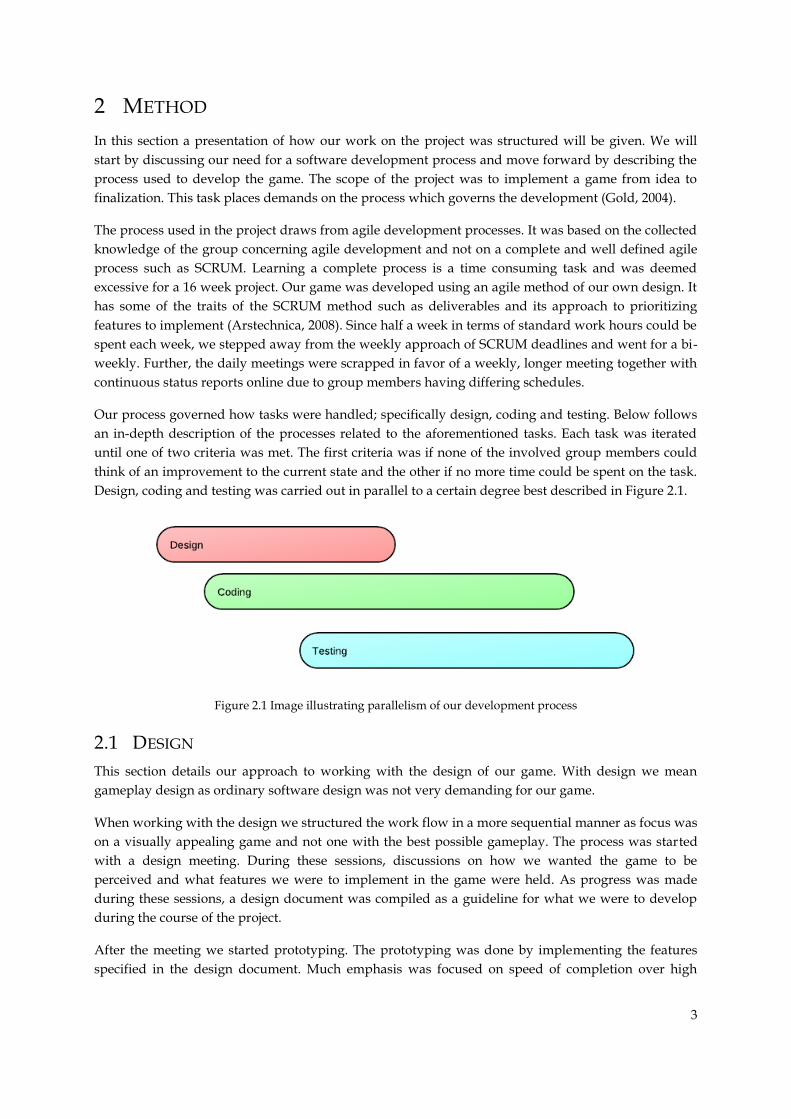
Design, coding and testing was carried out in parallel to a certain degree best described in Figure 2.1.

Figure 2.1 Image illustrating parallelism of our development process

2.1 DESIGN

This section details our approach to working with the design of our game. With design we mean

gameplay design as ordinary software design was not very demanding for our game.

When working with the design we structured the work flow in a more sequential manner as focus was

on a visually appealing game and not one with the best possible gameplay. The process was started

with a design meeting. During these sessions, discussions on how we wanted the game to be

perceived and what features we were to implement in the game were held. As progress was made

during these sessions, a design document was compiled as a guideline for what we were to develop

during the course of the project.

After the meeting we started prototyping. The prototyping was done by implementing the features

specified in the design document. Much emphasis was focused on speed of completion over high

4

production value. Prototyping was done to ensure that all ideas from our design meetings carried

over well into actual gameplay.

Once functional prototypes were made we began testing. During the testing phase, newly

implemented features were tried and feedback was gathered from the group. The feedback was

considered and a new prototype was made, new meetings held or the feature was accepted depending

on the feedback. Even though focus was not on making the gameplay perfect some adjustments had to

be done to ensure an enjoyable game.

When every feature had passed testing the design was to be considered final.

2.2 CODING

The approach we adopted to coding was heavily influenced by agile methods. Our coding process

was the one most similar to SCRUM. Coding here relates to creating code of high quality and not just

code that performs the correct task.

Every week a meeting was held. During a meeting, progress from the past week was discussed along

with problems encountered. Discussions were held on as to how to solve said problems. Every other

week, a priority list was made which defined what had to be done until the next priority list. The list

also governs what was to be done after high priority items had been implemented.

Between meetings we implemented the features described in the priority list. Due to working

intensively with iterative prototyping, functional code was prioritized over quality in our

implementations while the design phase was running in parallel.

Once coding had progressed far enough (see Figure 2.1) testing became a part of the weekly process as

well. Code testing was performed by checking for erroneous behavior in the game as opposed to unit

testing. An important part of testing was to identify features in need of optimization. This was because

properly working code was slow in some cases even after it had been implemented and tested. We

started to optimize the code after proper behavior was validated. Optimization was carried out by

identifying inefficient parts of code with the aid of timers. Said parts were subsequently improved to

behave in a more efficient manner.

During development, the code was generally iterated a few times before finally being optimized, after

which the code was considered final.

2.3 TESTING

Here testing towards the end of the project was the main focus, testing of code was touched upon in

the previous section. Testing in this case relates to the testing of the entire product.

A test meeting was held to tie the project together near the end of the coding process. During this test

meeting a play test was performed on simple maps to focus on important design decisions such as

controls. After the play test, discussions were held were thoughts on the current state of the game

were voiced and various solutions to perceived problems brought forward.

Following the discussion changes could be made either to the design or the code with the goal of

making the game more enjoyable. In our project we decided against large design changes during the

play test in order to meet our deadline.

5

We considered the game complete after all changes agreed upon during the test meetings were

implemented. If time was not a factor the process would have consisted of more than one test meeting

and more specialized play tests with focus on evaluating specific features.

2.4 OPTIMIZATION

This section will provide a more in-depth look at optimization. Optimization is to rewrite, remove and

structure code to improve its efficiency without affecting its functionality (Sedgewick, 1984). It is an

important part of software development where the software is time sensitive.

During our project, lighter optimization was done on a regular basis as part of the process of writing

code. Optimization was carried out to address an issue with low frame rates. In our project, we

focused on two types of optimization. The first one was optimization of the code structure. Large

sections of code were reduced to a manageable size by breaking out methods and structuring code

into classes. Little performance was gained from this but our goal was to make it easier to understand

and expand upon.

The second type of optimization was performance-oriented. This optimization began by identifying

which parts of the code needed to be optimized by extensively using timers to evaluate the time

needed to perform each method. When a time consuming method was identified, work began on

figuring out what caused the inefficiency, and if the time consumed was reasonable considering the

task. This involved looking at loops and call chains to find inefficient or erroneous code. Inefficiency

found during optimization included creating and initiating unnecessary variables, loading the same

resources multiple times, traversing large arrays when the sought item was available by simpler

means and code structures which forced setting of parameters back and forth instead of grouping all

code requiring the same parameters together.

6

3 GAMEPLAY DESIGN

Gameplay design is the definition of the content and rules of a game. It also describes how the game is supposed to look, feel and be experienced by the player. In this section we will present the choices of gameplay design implemented during development of the game. After this, we will explain our gameplay design choices and how they are associated with the uniqueness of our game.

3.1 INTRODUCTION

The aim of our gameplay design is to provide a gaming experience that is as enjoyable as possible to the players. We have used ourselves as the target audience for the game, and as such, we are judging the gaming experience from our own perspective. The purpose of our gameplay design is also to assure the competitiveness of our game on the video games market. This is done by making the product unique and niche, which has to be drawn from our gameplay design.

When determining the competiveness of our game, we only need to make comparisons to other similar games within the market on which our game is planned to be sold. Our target audience will be used to determine which market this will be, and as we, ourselves, act target group, we know that we want the game to be sold via the digital distribution service Steam (Steam, 2012). The uniqueness of our game can as such be measured by comparison to similar games within Steam’s games catalogue.

3.2 STUDY OF DESIGN CHOICES

To be able to measure the uniqueness of our game, a study (Appendix A) of similar games in Steam’s games catalogue was conducted. The study investigates which gameplay design choices, characterizing to our game, that are also made in these games. Similar games are defined as racing games, space games, and aircraft flight games. Only the top games in each category were studied since we were aiming for a unique product among competitive games. This was based on metacritic’s Metascore, which is “a weighted average of reviews from top critics and publications” (Metascore, 2010). The gameplay design choices are listed in the following sections.

1. Free three-dimensional movement is what we call the ability to control the player inside the game

equally in every dimension of the 3D-world.

2. Three-dimensional navigation tools are our name on features inside the game that help the player

navigate 3D space.

3. Guide lines are as guide rails, which are explained in section 3.4.1, but are only drawn statically on the

track.

4. We say that a player has free movement if it is not prevented by the environment or the game

mechanics to move to any location.

5. Drag is explained in section 3.4.2. We call a player’s drag long drag if the portions of it last after the

player has left their vicinity. We call our drag long drag in the appendix since we are comparing to

games in which the drag is significantly shorter and thus affects gameplay in another way.

6. Multiplayer means that the same game can be played by multiple players in real-time.

3.3 RACING IN SPACE

Racing is a subgenre of games where the player is participating in competitive races. Races in our game are located in a space environment and the players are competing with spaceships.

7

3.4 PLAYER MOVEMENT

In our game, the player is allowed to move freely in any direction. The player is allowed to accelerate, break, turn and roll. When turning, the player’s velocity will slowly change until the velocity has the same direction as the player. The spaceship is controlled by a keyboard and mouse setup. The player will accelerate with the W-key, break with the S-key, roll left with the A-key and roll right with the D-key. The player will turn up, down, left and right by moving the mouse in the respective direction.

3.4.1 GUIDE RAIL

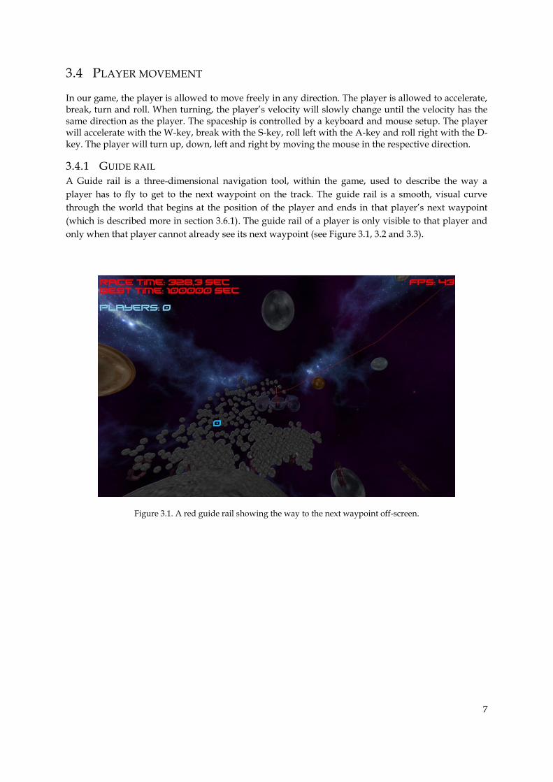
A Guide rail is a three-dimensional navigation tool, within the game, used to describe the way a

player has to fly to get to the next waypoint on the track. The guide rail is a smooth, visual curve

through the world that begins at the position of the player and ends in that player’s next waypoint

(which is described more in section 3.6.1). The guide rail of a player is only visible to that player and

only when that player cannot already see its next waypoint (see Figure 3.1, 3.2 and 3.3).

Figure 3.1. A red guide rail showing the way to the next waypoint off-screen.

8

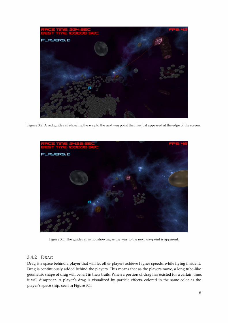
Figure 3.2. A red guide rail showing the way to the next waypoint that has just appeared at the edge of the screen.

Figure 3.3. The guide rail is not showing as the way to the next waypoint is apparent.

3.4.2 DRAG

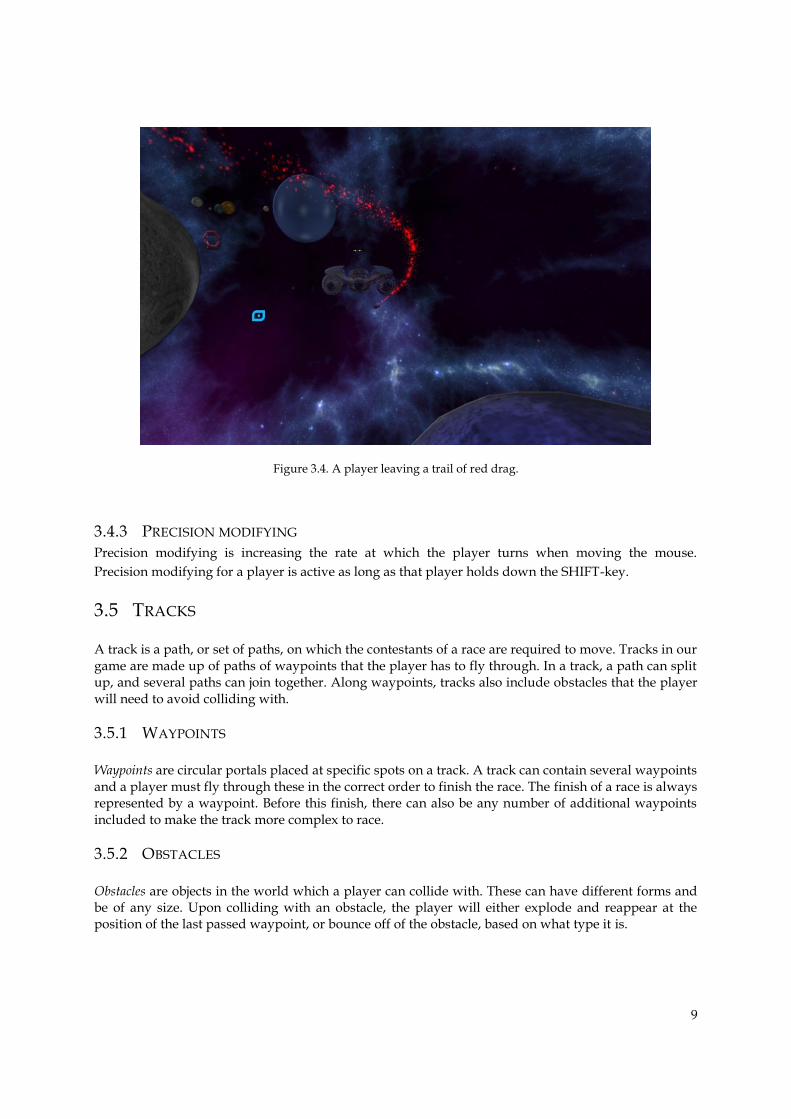
Drag is a space behind a player that will let other players achieve higher speeds, while flying inside it.

Drag is continuously added behind the players. This means that as the players move, a long tube-like

geometric shape of drag will be left in their trails. When a portion of drag has existed for a certain time,

it will disappear. A player’s drag is visualized by particle effects, colored in the same color as the

player’s space ship, seen in Figure 3.4.

9

Figure 3.4. A player leaving a trail of red drag.

3.4.3 PRECISION MODIFYING

Precision modifying is increasing the rate at which the player turns when moving the mouse.

Precision modifying for a player is active as long as that player holds down the SHIFT-key.

3.5 TRACKS

A track is a path, or set of paths, on which the contestants of a race are required to move. Tracks in our game are made up of paths of waypoints that the player has to fly through. In a track, a path can split up, and several paths can join together. Along waypoints, tracks also include obstacles that the player will need to avoid colliding with.

3.5.1 WAYPOINTS

Waypoints are circular portals placed at specific spots on a track. A track can contain several waypoints and a player must fly through these in the correct order to finish the race. The finish of a race is always represented by a waypoint. Before this finish, there can also be any number of additional waypoints included to make the track more complex to race.

3.5.2 OBSTACLES

Obstacles are objects in the world which a player can collide with. These can have different forms and be of any size. Upon colliding with an obstacle, the player will either explode and reappear at the position of the last passed waypoint, or bounce off of the obstacle, based on what type it is.

10

3.6 MULTIPLAYER

Multiplayer is the possibility for different players to play with, or against each other in a game. Multiplayer in our game lets a player race against other players in real-time. Players can see each other and be affected by each other’s drag.

3.7 DISCUSSION AND RESULT

In this section the result from our gameplay design is discussed in several subsections.

3.7.1 DISCUSSING RACING IN SPACE

When starting the project, none of us knew anything about model animation. Because of this, we wanted to avoid working with animations as much as possible during development. Racing games generally require few animations. On a car, it can be enough with animating the wheels turning. In a first person shooter game, on the other hand, a lot of character animations are needed. Hence, we decided on developing a racing game.

The reason for developing a racing game set in space was that we would not have to create as many complex models, such as trees or detailed houses, to fill the world with.

3.7.2 DISCUSSING THREE-DIMENSIONAL MOVEMENT

Since the game is set in space, free three-dimensional movement adds to the realism of the game, as a space ship’s movements in zero gravity can be expected to behave the same when flying in any direction. An open world is also motivated to use in space as there, in reality, are very few objects in space that could restrict a space ship in its movements.

The combination of an open world and free three-dimensional movement is a very unique design decision when used together with a racing game. As seen in our study (Appendix A), none of the investigated games, uses this combination.

3.7.3 DISCUSSION CONCERNING AN OPEN WORLD

All racing games included in our study (Appendix A) are in some way restricting the player from deviating too much from the racing track. This can be good as it keeps players from getting lost in what would otherwise be a fully open world. Restrictions like these are often accomplished by placing physical, impassible walls around the track, such as fences (FlatOut 2), rocks (Need for Speed: Hot Pursuit) or tightly placed trees (DiRT 3). All of these are probable to find around real world tracks and as such do not decrease the realism of the game. In some cases though, the tracks of a game do not provide any possibility for a natural occurring boundary. In SkyDrift for instance, large parts of the tracks are open air, and as such, natural boundaries are difficult to motivate without lowering the sense of realism in the game. To alleviate this problem, SkyDrift uses invisible walls which will only affect a player once he/she deviates too much from the track to actually hit the wall. This would also be the common method of use in a game where tracks are located in space.

Though invisible walls are subtle in the manner recently described, they do prevent a player from moving where it would normally be possible to go. Because of this, the player’s sense of free movement will be removed when they know that invisible walls are being used. This can be confusing for the player when controlling a vehicle or craft that would otherwise allow free movement, and as a result, lower the overall immersion for that player.

As we want our game to be unique and aim to provide our players with an immersive gaming experience, we chose our game to be set in an open world where no tracks would include any invisible

11

walls or similar restrictions. This choice introduces the possibility for players to lose their heading relative to the track, a problem we solved by using guide rails.

3.7.4 DISCUSSING PLAYER MOVEMENT

We wanted to implement a method of player control and movement that we knew many players within our target audience were accustomed to. We decided to use controls that were similar to those used in ordinary car racing games, but with an influence of realistic space movement. Thus, we could let the controls feel familiar to our players while also giving movement a unique feeling in our game.

Our game uses both keyboard and mouse configuration for controls. This is because using the mouse for turning will give players a more precise tool than what a keyboard otherwise would have offered. With this method follows an issue of space for moving the mouse, however. Our solution to this issue is precision modifying, and the issue itself will be further described under that discussion (3.8.6).

3.7.5 DISCUSSING GUIDE RAILS

The use of guide rails in our game is important since we are allowing full three-dimensional movement as well as an open world while still encouraging players to fly fast. Because of this, it is possible for a player to get into a position where it is, for instance, facing away and flying from the track. In these situations it can be difficult for the player to quickly determine its bearing relative to the track and also to know where the next waypoint is located. This can lead to the player missing parts of the track or simply flying so far away from it that the player cannot find his/her way back.

This problem can be alleviated by the use of three-dimensional navigation tools. One popular such method is being used in all space games with free three-dimensional movement, included in our study. This method is based on drawing markings or arrows on the player’s heads-up display. These markings, however, only tells in which direction an object is located, and does not describe any other movement specifics, such as how fast the player must turn to reach that object.

Guide rails are our own method of providing a three-dimensional navigation tool, very much inspired by the guide- or racing help lines that can be turned on in certain simulation racing games such as F1 2011. These help lines are drawn statically on the ground of the track to show the optimal way of racing. Like these, guide rails are meant to somewhat represent a possible flight path that the player can take, and as such, they will act as a good measurement for what movement actions must be taken. The difference between guide rails and the help lines however, is that guide rails are actively updated to always originate from the players position.

3.7.6 DISCUSSING PRECISION MODIFYING

In our game, we want players to be able to turn with high precision, should they want to aim for an object far away. We also want the players to be able to make really quick turns if they, for example, would need to turn around fast. However, players often have limited space to move their mouses around and because of this; it can be difficult to adhere to both precise and quick mouse controls. This is why the game has precision modifying which enables a player to, on demand, accelerate the speed at which the player will turn.

3.7.7 DISCUSSING DRAG

Drag is used to let players that have fallen behind in the race, catch up to players in front. This will give a more tense feeling to the races as experienced players will still have to focus on playing well, as less experienced players might still catch up. Less experienced players will also be encouraged to focus more on playing well as there is still a chance that they can pass the more skilled players if they do.

12

3.7.8 DISCUSSING WAYPOINTS

The motivation behind waypoints is to give the player many short-term aims during a race. In order to reach the finish in the shortest time possible, the player must focus on finding the optimal way of flying through each waypoint. In racing games the track is usually set up of different kinds of turns which the player has to aim to corner in the most optimal way. By introducing waypoints we can also provide this kind of depth to our game.

To further enhance the depth of a race, we allow separate waypoints to vary in size to encourage players to act in a certain way, such as flying slower when trying to go through small waypoints.

3.7.9 DISCUSSING OBSTACLES

In our game, obstacles serve to make the tracks more technical. Between each waypoint, the players must choose how to fly around several possible obstacles, and try to find the fastest route through these. Obstacles also increase the tension of the game as players colliding with them will be set off their path, and possibly enable other players to pass them.

3.7.10 DISCUSSING MULTIPLAYER

Our game has real-time multiplayer to allow for players to compete against each other. Every racing game in our study except GRID, also have real-time multiplayer. GRID, on the other hand, has computer controlled players, and as such also provides real-time opponents to the player. Being able to compete against other humans, or computer controlled players, seems like a popular design choice in all other racing games. We also view it as an important feature to have in our game to avoid losing competitiveness.

3.7.11 CONCLUSION

The gameplay design choices implemented in our game have made it both enjoyable and unique. The game is enjoyable since several design choices add tension to the game while others provide immersion to the player. The game is also unique as many of the design choices made are not seen in any similar games on the market of interest. As such, the aims of our gameplay design were fulfilled.

13

4 GRAPHICS

Graphics in computer games relates to how the graphics pipeline renders a two-dimensional image in real-time. Therefore a brief explanation of the graphics rendering pipeline will follow to facilitate understanding of the later sections on graphic effects.

4.1 THE GRAPHICS PIPELINE

The graphics rendering pipeline is a three-stage process which consists of the application, geometry and rasterizer stages. As data passes through these stages, an object defined in code is transitioned to a 2D representation and finally drawn on the screen. Any program that handles objects in a three dimensional space needs to interact with the graphics rendering pipeline (Akenine-Möller et al., 2008).

4.1.1 APPLICATION STAGE

The application stage holds all work done on the CPU and it determines what primitives are to be sent to the geometry stage for further processing (Akenine-Möller et al., 2008).

4.1.2 GEOMETRY STAGE

The geometry stage places and orders all the objects present in the current game scene. For an object, this is done by applying transformation matrices to the object’s coordinates, thus placing them in the ‘world space’ as opposed to their origin in the ‘model space’. The world space differs from the model space in that all objects have unique coordinates and they are all placed in the same space. When the objects have their place in the world matrix, the objects that we see must be determined. This is done with the aid of the view frustum. The view frustum dictates what we see and what we do not see. Any object inside the frustum is visible and all objects outside of it are not. Objects that are partially inside are clipped (Akenine-Möller et al., 2008).

When the objects we can see have been determined, they are moved together with the camera with transformation matrices so that the view frustum has its origin in the center of the coordinate system and the camera is looking in the direction of the negative z-axis. This is done to simplify the mathematical operations needed later. This new space is called the ‘eye space’. In the eye space the region containing the objects that are visible is a subsection of a pyramid. This means that distance between two coordinates close to the camera appear to be of greater length than the same coordinates further away from the camera. To adjust this, the objects are projected into the so called ‘clip space’ where they are clipped against a unit cube. From the clip space the objects are then mapped to the screen. In this stage the z-coordinates describing depth are still kept. Nothing has yet been drawn but instead we have a set of three dimensional coordinates describing where objects are on the screen together with information relating to said objects’ color and other properties (Akenine-Möller et al., 2008).

4.1.3 RASTERIZER STAGE

The final stage; the rasterizer stage, is where pixels are drawn on the screen. The process begins by linking all vertices, which make up the objects to be drawn, to form triangles. Once all vertices are part of a triangle the triangle traversal stage commences. Triangle traversal creates so called fragments for every pixel found to be inside a triangle. A fragment contains coordinates relating to the screen, the depth value (z-coordinate) and data pertaining to its color and texture-related data. When this is done, the image is drawn in a fragment shader. The shader calculates the final color of each fragment based on the texture, lighting and other graphical effects (Akenine-Möller et al., 2008).

14

4.2 GAUSSIAN BLUR

A filtering technique used in several of our graphic effects is Gaussian blur and is introduced here.

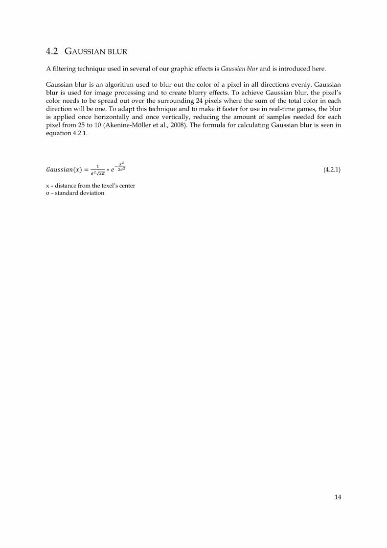
Gaussian blur is an algorithm used to blur out the color of a pixel in all directions evenly. Gaussian blur is used for image processing and to create blurry effects. To achieve Gaussian blur, the pixel’s color needs to be spread out over the surrounding 24 pixels where the sum of the total color in each direction will be one. To adapt this technique and to make it faster for use in real-time games, the blur is applied once horizontally and once vertically, reducing the amount of samples needed for each pixel from 25 to 10 (Akenine-Möller et al., 2008). The formula for calculating Gaussian blur is seen in equation 4.2.1.

√

(4.2.1)

x – distance from the texel’s center σ – standard deviation

15

4.3 CULLING

In computer graphics, culling is the same thing as in herding where you separate individuals from a flock. The flock in this context is the scene we want to render and what we remove are the portions of the scene that are not considered necessary for the final image like objects currently outside of the screen space. Examples of such techniques are backface culling, view frustum culling and occlusion culling (Akenine-Möller et al., 2008).

4.3.1 BACKFACE CULLING

Solid objects may occlude themselves. For instance, when observing a solid object such as a sphere, the backside or approximately half of the sphere will not be visible and there is no need to process the triangles that are not visible.

The key to implementing backface culling is to find the backfacing polygons. One technique is to compute the normal of the projected polygon in two-dimensional screen space: n = (v1-v0) x (v2- v0). This normal will either be (0,0,a) or (0,0,-a), where a > 0. If the negative z-axis is pointing into the screen, the first result indicates a frontfacing polygon (Akenine-Möller et al., 2008). Another way to determine if a polygon is backfaced is to create a vector from an arbitrary point on the plane in which the polygon lies to the camera position and then compute the dot product of this vector and the normal of the polygon. If the value is negative, the angle between the two vectors is greater than π/2 radians. This results in that the polygon is not facing the camera position and therefore it can be determined as a backfacing polygon (Akenine-Möller et al., 2008).

4.3.2 VIEW FRUSTUM CULLING

The term frustum in computer graphics is commonly used to describe the three dimensional region which is visible on the screen. It is formed by a clipped rectangular pyramid that originates from the camera and is called the ‘view frustum’. The idea behind view frustum culling is to avoid processing objects which are not in the camera’s field of view. This can be done by using bounding boxes or spheres on objects. These can be used to look for intersections with the view frustum. Any objects intersecting with the view frustum is drawn as it is at least partially visible (Akenine-Möller et al., 2008).

The size of the frustum has to be taken into consideration, as the size increases, the efficiency degrades as more objects may be found in the frustum and therefore processed. With a view frustum that is too small, objects will show up in full size near the camera. For instance, in a space game, a small frustum could lead to planets that are expected to be seen at greater distances, to show up at what appears as a short distance from the camera.

4.3.3 OCCLUSION CULLING

If there are objects hidden behind other objects, the occlusion culling algorithms try to cull away those occluded objects. An optimal occlusion culling algorithm would render only those objects that are visible.

Modern GPUs support occlusion culling by letting users query the hardware to find out whether a set of polygons is visible when compared to the current contents of the Z-buffer (which contains the depth values of objects in the scene). This set of polygons often forms the bounding of an object. If none of these polygons are visible then that object can be culled. The hardware counts the number of pixels, n, in which these polygons are visible and if n is zero and the camera is not inside the bounding, the object does not need to be rendered. A threshold for the number of pixels may be set, comparing if n is smaller than this threshold value to find if it is likely to contribute to the final image or otherwise be discarded.

16

4.3.4 METHOD: OUR IMPLEMENTATION

We have used the support for culling that comes with the XNA 4.0 framework which is backface culling and view frustum culling.

4.3.5 RESULTS

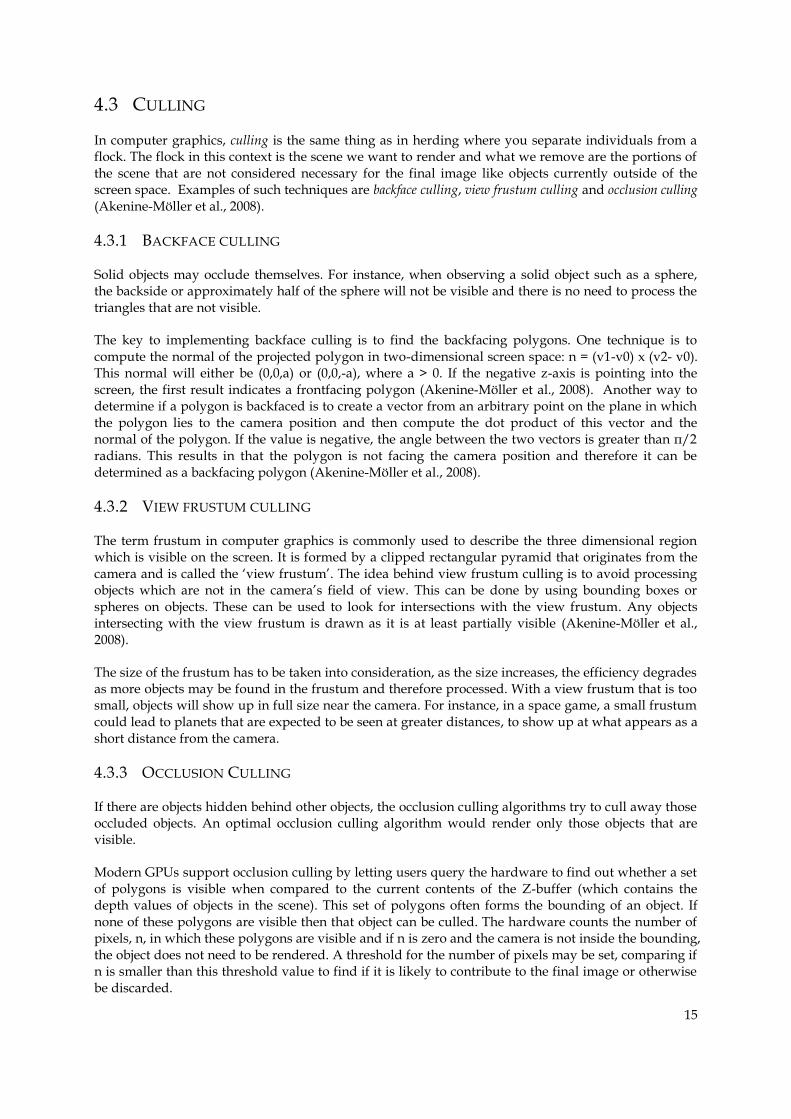
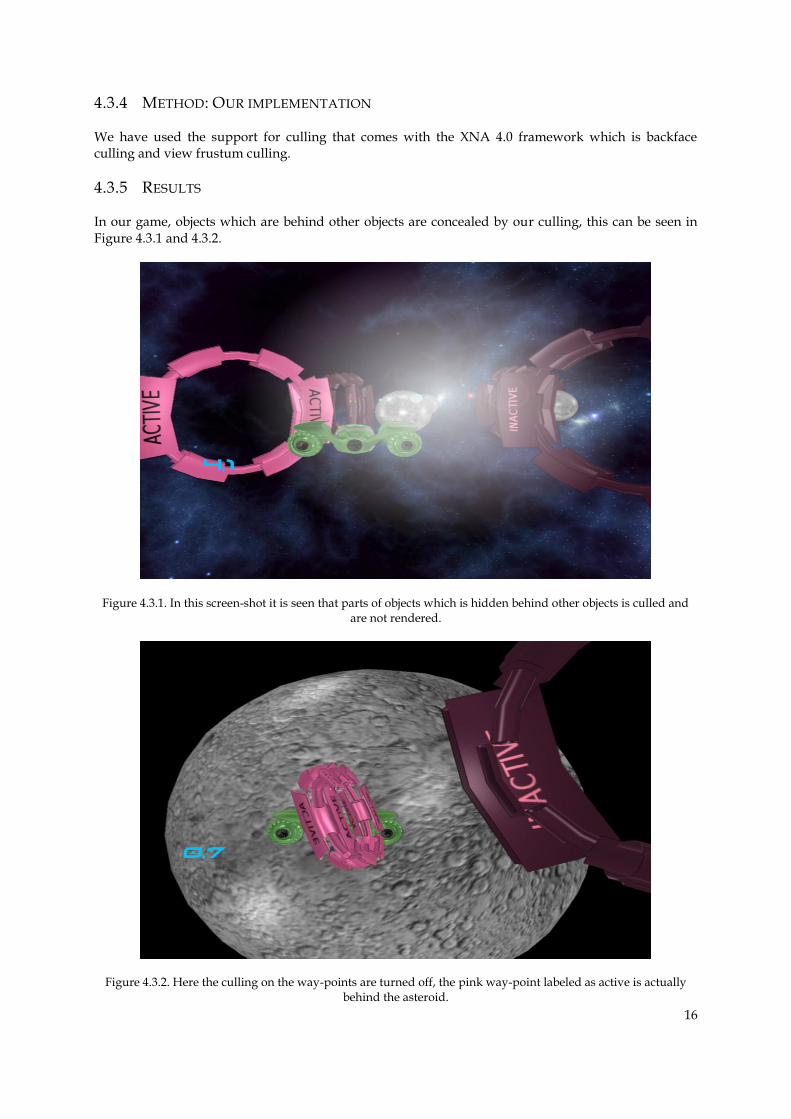
In our game, objects which are behind other objects are concealed by our culling, this can be seen in Figure 4.3.1 and 4.3.2.

Figure 4.3.1. In this screen-shot it is seen that parts of objects which is hidden behind other objects is culled and are not rendered.

Figure 4.3.2. Here the culling on the way-points are turned off, the pink way-point labeled as active is actually behind the asteroid.

17

4.3.6 DISCUSSION

Our game does not include many objects that may conceal each other and therefore using the provided culling support from XNA 4.0 has been sufficient. In this stage of our development there has been no need to implement advanced culling algorithms, since our game so far is able to render spaceships, planets, waypoints and a lot of asteroids in our scene without any major FPS drops. In our optimizations tests where we increased the number of asteroids, we noticed a greater degree of performance loss that may be because of inferior culling. This could however have been because the asteroids are smooth spheres that consist of a lot of polygons which cause increased workload on the GPU.

18

4.4 SHADING

Shading is the process of calculating the color of materials and textures depending on the lights present in the scene. There are three major algorithms for calculating shading: Flat shading, Gouraud shading, Phong shading and a variation on Phong shading called Blinn-Phong shading.

4.4.1 INTRODUCTION

To render an object that consists of several polygons and to make it appear as one smooth surface, shading is used. All the objects in a scene have a material color which is calculated by using shading. Material colors are typically defined using Diffuse, Ambient, Specular and Emissive color components. These are combined to give the final material color in RGB values. The color components are an approximation of how colors appear in the real world and are calculated differently depending on the shading technique used.

Material ColorRGB = DiffuseRGB + AmbientRGB + SpecularRGB + EmissiveRGB

(Akenine-Möller et al., 2008)

4.4.1.1 DIFFUSE

Diffuse color is the basic color of the material and is the result of direct light from a light source in the scene. Using only the diffuse component gives a flat impression of the object. Diffuse color is a representation of light in the real world that has undergone transmission, absorption and scattering in an object surface. Transmission is when the light photons are scattered inside the material, absorption is when the material has absorbed some amount of light photons and scattering is when some of the photons are scattered or reflected in different directions. (Akenine-Möller et al., 2008)

4.4.1.2 AMBIENT

Ambient color is usually a mix between diffuse and specular color and is essentially the color that the material has when it is in shadow or is only lit by indirect light. It occurs when a material is lit by ambient light. (Akenine-Möller et al., 2008)

4.4.1.3 SPECULAR

Specular color is when the light photons are reflected by a material. The more a material reflects the photons, the glossier the material appears to be. (Akenine-Möller et al., 2008)

4.4.1.4 EMISSIVE

Emissive color is the color that a material emits or the self-illumination of the material. (Akenine-Möller et al., 2008)

4.4.2 FLAT AND SMOOTH SHADING

There are two main subcategories in shading; Flat shading and Smooth shading. The two algorithms used most extensively today for smooth shading are Gouraud shading and Phong shading. There are a number of variations of them used in real-time games; one is Blinn-Phong shading. Flat shading is the original shading technique which has evolved to the smooth shading techniques used today in most games.

19

4.4.2.1 FLAT SHADING

Flat shading is computed for each triangle in a scene and only considers the normal that each triangle has for calculating the color depending on the light direction. The visual result of flat shading is that all the triangles are drawn flat making the triangle edges visible. The algorithm does not use much of the GPU but gives the objects a blocky appearance. (Akenine-Möller et al., 2008)

4.4.2.2 SMOOTH SHADING

Smooth shading is a technique which produces continuously curved surfaces even with low-polygon models. Smooth shading is computed per vertex or per pixel to approximate the color of lit objects. Three different algorithms for creating smooth shading will be presented; Gouraud shading, Phong shading and Blinn-Phong shading.

4.4.2.3 GOURAUD SHADING

Gouraud shading, developed by Gouraud (1971), creates smooth shading and hides the polygon edges. This is done by creating an average normal for each vertex to mimic a smooth curved surface’s shape without having to increase the amount of polygons in the model. Gouraud shading is done in the vertex shader and calculates the color value per vertex. (Akenine-Möller et al., 2008)

Gouraud shading cannot handle specular highlights very well in dynamic scenes unless the number of polygons in the models is increased.

4.4.2.4 PHONG SHADING

Phong shading, developed by Phong (1973), gives smooth surfaces with realistic specular high-lights, this is done by accounting for the viewer position when calculating the shading. The formula for calculating the specular component in Phong shading is displayed in equation 4.4.1. An approximation of this formula is used when calculating the shading in a game.

(4.4.1)

Sp – the resulting specular color Cp – reflection coefficient of the object at point p for a certain wavelength i – incident angle d – environmental diffuse reflection coefficient W(i) – gives the ratio of the specular reflected light and the incident light s – angle between the direction of the reflected light and the view vector n – models the specular reflected light for each material

Phong shading is implemented in the pixel shader and the angle between the view vector and the reflection vector needs to be recomputed for every pixel, causing it to render a realistic scene but is more GPU-intensive than Gouraud shading. (Akenine-Möller et al., 2008)

4.4.2.5 BLINN-PHONG SHADING

Blinn-Phong shading is a smooth shading algorithm based on Phong-shading but with more accurate results. The result generated causes a higher computational cost on the GPU due to that the shading is computed on a halfway vector (equation 4.4.2) instead of using the reflection vector.

| | (4.4.2)

H – halfway vector L – light vector V – view vector

20

By treating the light sources as being at an infinite position from the shaded surface, the Blinn-Phong shading algorithm can be calculated more efficiently. (Blinn, 1977)

4.4.3 METHOD: OUR IMPLEMENTATION, PHONG SHADING

In our project we chose to use Phong shading which is used in real-time games. The implementation was easy due to the many variations of Phong-shading available on the web which could guide us.

4.4.4 RESULT

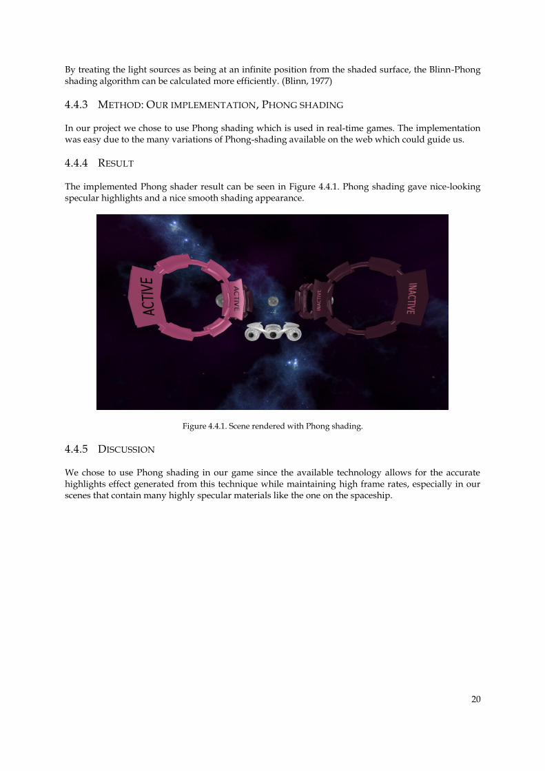
The implemented Phong shader result can be seen in Figure 4.4.1. Phong shading gave nice-looking specular highlights and a nice smooth shading appearance.

Figure 4.4.1. Scene rendered with Phong shading.

4.4.5 DISCUSSION

We chose to use Phong shading in our game since the available technology allows for the accurate highlights effect generated from this technique while maintaining high frame rates, especially in our scenes that contain many highly specular materials like the one on the spaceship.

21

4.5 MULTIPLE LIGHT SOURCES

Using multiple light sources in a game can cause performance issues and is a common problem for real-time rendering in 3D. There are several techniques that can be used to accomplish the calculation of lighting, shading and shadows for a scene in real-time. Single-pass lighting, Multi-pass lighting, Forward shading and Deferred shading will be explained in the following section.

4.5.1 INTRODUCTION

Having multiple light sources in a scene requires large amounts of memory and each frame needs to store two textures for each light: one texture with the light information, which includes the color of the light and the area that it affects, and one texture that contains the depth map from light source’s point of view.

Using multiple light sources is essential for our game since we want to use lights to make the scene more visually appealing. There are three main types of light that can be used in a scene; point lights, directional lights and spot lights.

4.5.1.1 POINT LIGHT

A point light is a light source that emits light evenly in all directions from a center point. Point lights are represented in a game by having the center of the light be in the middle of a box; using the six sides of the box to contain light maps and shadow maps for all the different directions. (Microsoft Dev center, 2012)

4.5.1.2 DIRECTIONAL LIGHT

A directional light has no position but instead only a direction, a scene is lit evenly from that direction. (Microsoft Dev center, 2012)

4.5.1.3 SPOTLIGHT

A spotlight consists of a point of origin and a direction. The light illuminates a cone-shaped region from the spotlight’s position in a specific direction. A constraint is used to determine the size of the cone. (Microsoft Dev center, 2012)

4.5.2 SINGLE-PASS LIGHTING

Single-pass lighting uses only one shader which is the simplest way to handle multiple light sources. However, it is also the most limiting technique. In single-pass lighting the light contributions are calculated in one shader for each object in the scene which makes it hard to handle several different light sources. To handle several different light sources and several different materials in that one shader will make it very complicated. Using single-pass lighting limits the scene to eight lights, as more than eight lights lowers the frame rate significantly. (Zima, 2010)

4.5.3 MULTI-PASS LIGHTING

In multi-pass lighting, each light has its own shader which enables the use of several different kinds of lights. Using several shaders also enable more light sources in a scene but the technique is limited by the fact that each object needs to be rendered for each light that is affecting it, causing it to be very inefficient. This can cause all objects in a scene to be required to be rendered by all light sources in the scene. (Zima, 2010) In games it is common to use several different materials in a scene, combining them with different shaders for each light source can cause one shader to be needed for each material

22

and for each light source. The amount of shaders required for accurate lighting on different materials may thus be very large (sometimes over 1000). (Akenine-Möller et al., 2008)

4.5.4 FORWARD SHADING

Forward shading, or Forward rendering, is a four-step process and is the process done within a single shader. Forward shading is the most common way to render real-time games and with it single-pass lighting or multi-pass lighting is used.

The four steps in Forward shading are as follows:

1. Compute the geometry shapes. 2. Determine surface material characteristics (e.g. normals and specularity). 3. Calculate the incident light. 4. Compute how the light effects the scene’s geometry.

When using deferred shading, the four steps are divided into the first two steps which are performed in one shader and the second two in a secondary shader. These two parts are calculated in different rendering pipelines (Koonce, 2008).

4.5.5 DEFERRED SHADING

Deferred shading, or Deferred rendering, is a technique which uses as few draw calls as possible for all objects in a scene. Each object is rendered once into a geometry buffer (G-buffer) which saves information such as position, normal, color and specularity for each pixel. The G-buffer is then used for applying the light contributions and shadows as a post-processing effect per pixel. This reduces the amount of draw calls significantly as there will only be a need to render the number of objects in the scene once plus the number of lights in the scene (if shadows are used more draw calls are needed) and there is no need to render any objects that are not currently visible in the screen space (Shishkovtsov, 2005).

Deferred shading with more complex effects can outperform a forward renderer using simple effects making it efficient in many cases (Shishkovtsov 2005). The technique is used in several modern games, Battlefield 3 and Need for Speed: The run are two examples (Ferrier and Coffin, 2011).

An advantage with deferred shading is that the fragment shading is done once per pixel per post-process effect in the visible scene, causing the amount of rendering computations to have a predictable, upper bound. Another advantage is that any computations needed for lighting is done only once per frame with the help of the light map (a light map contains all information regarding lighting like color and shadows). Deferred shading also separates light computations and material computations. This causes each new type of light source to require only one new shader, keeping the number of shaders for a game low. 50 or more dynamic lights can be rendered simultaneously in a scene while keeping an acceptable frame rate in real-time rendering. The amount of light sources is only limited by the amount of shadow-casting lights that are to be used in the scene. Having more shadow-casting lights causes more strain on the GPU since more computations are needed to create the shadow effect. This can be solved by allowing only specific light sources in the scene to be able to generate shadows. (Shishkovtsov, 2005)

A few disadvantages with deferred shading are that it is difficult to handle transparent objects in the scene since it is not possible to allow alpha blending on objects saved in the G-buffer. One way to solve this is to render all of the transparent objects last when the deferred shading is finished. Another disadvantage is that the technique uses a higher memory bandwidth compared to other techniques, meaning that a game will not be able to run on outdated graphics hardware.

23

Deferred shading does not support hardware antialiasing (AA) which is another disadvantage since AA is used extensively in graphic effects to improve appearance. The solution to this problem is to add AA as a post-process once the deferred shading has finished rendering the scene. (Koonce, 2008)

4.5.6 METHOD: OUR IMPLEMENTATION, DEFERRED SHADING

In our implementation of deferred shading, we use a multiple render target with three render targets. The first render target consists of four 32-bit values for each pixel in the screen space. In first three 32-bit slots, the albedo values (texture colors) are stored and in the fourth slot the first specularity value of the pixel is stored. The second render target consists of four 32-bit values where the first three slots contain the normal values for all pixels in the scene and the fourth value contains the second specularity value for that pixel. The specularity values are used in our implementation to identify different materials in the scene. The third render target consists of a single 32-bit value that contains the depth value for all the pixels in the scene.

Below is a short summary of the algorithm we used to implement deferred shading in our game.

1. Clear the G-buffer between each frame. 2. Create the G-buffer containing all of the values (position, normal, color and optional values)

for the pixels in the scene. 3. Create the shadow maps. 4. Create a light map for all the light sources in the scene. 5. Combine the shadow map, the light map and the color for each pixel in the scene into a

texture which is then displayed

When the scene has been rendered once and the pixel information is saved to the G-buffer, the shadow maps are created (shadow maps will be explained in section 4.6). Scene geometry affected by shadows is then rendered once for every light that casts shadows and a shadow map for each light is created and stored. The next step creates the light maps for each light in the scene. The light maps contain the lighting information for each light; the color, intensity of the light and the shadows produced by that light source. This is done for each light using the stored information in the G-buffer and the shadow maps for each light. The data is then combined into one light map for the entire scene. The final step is to combine the G-buffer scene’s values with the light map and then display the scene on screen.

4.5.7 RESULT

The results can be seen in Figure 4.5.1: the data saved in the G-buffer, the combined light maps and the final scene. The results from the frame rate test can be seen in the Table 4.5.1.

24

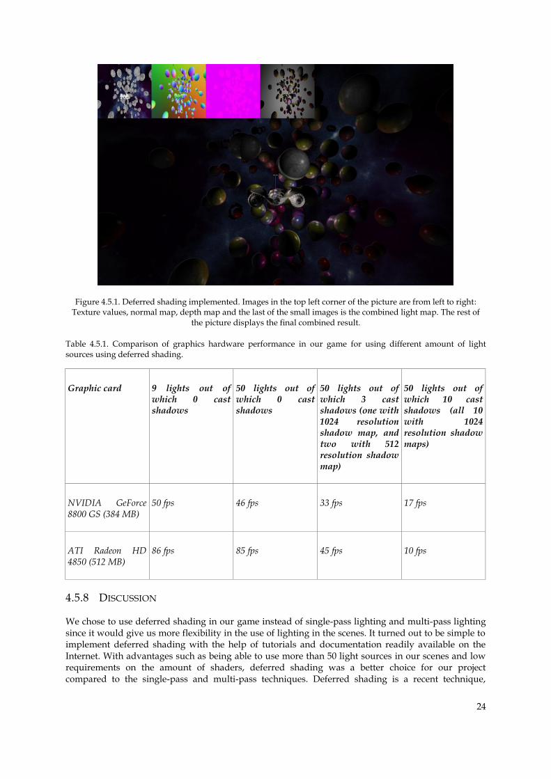
Figure 4.5.1. Deferred shading implemented. Images in the top left corner of the picture are from left to right: Texture values, normal map, depth map and the last of the small images is the combined light map. The rest of

the picture displays the final combined result.

Table 4.5.1. Comparison of graphics hardware performance in our game for using different amount of light sources using deferred shading.

Graphic card 9 lights out of which 0 cast shadows

50 lights out of which 0 cast shadows

50 lights out of which 3 cast shadows (one with 1024 resolution shadow map, and two with 512 resolution shadow map)

50 lights out of which 10 cast shadows (all 10 with 1024 resolution shadow maps)

NVIDIA GeForce 8800 GS (384 MB)

50 fps 46 fps 33 fps 17 fps

ATI Radeon HD 4850 (512 MB)

86 fps 85 fps 45 fps 10 fps

4.5.8 DISCUSSION

We chose to use deferred shading in our game instead of single-pass lighting and multi-pass lighting since it would give us more flexibility in the use of lighting in the scenes. It turned out to be simple to implement deferred shading with the help of tutorials and documentation readily available on the Internet. With advantages such as being able to use more than 50 light sources in our scenes and low requirements on the amount of shaders, deferred shading was a better choice for our project compared to the single-pass and multi-pass techniques. Deferred shading is a recent technique,

25

making it interesting to implement and study. Deferred shading made it simple to implement all of our post-process effects.

Our first implementation used 64-bit values instead of the current 32 bits for the multiple render targets but it was discovered that less powerful graphics hardware did not have enough memory to use 64-bit values so we decided to change to 32-bit values. Using 32 bits made it possible to use the same multiple render target setting on all graphics hardware available to us during the development process.

We also had some problems using a skysphere together with deferred shading since we did not want the lights to affect the skysphere. The problem was solved by using our extra specularity values for identifying the skysphere, causing the light shaders to ignore it.

For future improvements and to further increase the performance of our deferred shader, a variation called tile-based deferred shading could be implemented. In tile-based deferred shading the scene is divided into zones so that when creating the shadow maps for each light, only the affected geometry needs to be considered and not the entire scene for each shadow casting light source. This would allow for more shadow-casting light sources.

26

4.6 SHADOWS

Shadows in games provide a player with visual clues about the placement of objects and adds to the realism of the game (Akenine-Möller et al., 2008). This section covers the major shadow techniques used in real-time games: Projected planar shadows, Shadow volumes and Shadow maps. Two different kinds of shadow maps are then presented; Variance shadow maps and Exponential shadow maps. The results from the implementation in the game is then viewed and discussed.

4.6.1 INTRODUCTION

Shadows in the real world have sharp or soft edges. An object casts sharp shadows when the light source is distant from the object, e.g. the sun, whereas soft shadows are cast when the light source is closer. This is simulated in real-time games by different techniques.

The main techniques considered for producing shadows in games are projected planar shadows, shadow volumes and shadow maps and these techniques will all be presented in this section.

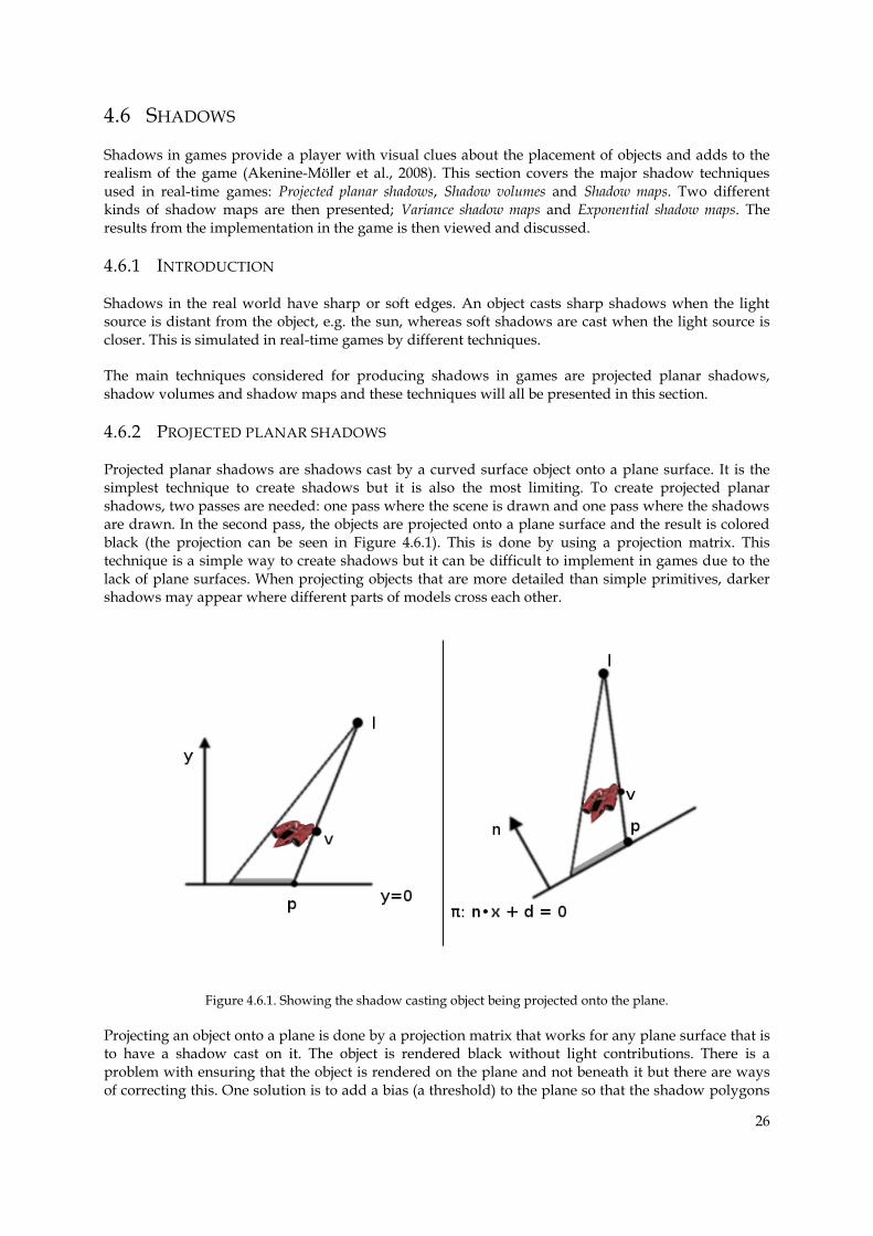
4.6.2 PROJECTED PLANAR SHADOWS

Projected planar shadows are shadows cast by a curved surface object onto a plane surface. It is the simplest technique to create shadows but it is also the most limiting. To create projected planar shadows, two passes are needed: one pass where the scene is drawn and one pass where the shadows are drawn. In the second pass, the objects are projected onto a plane surface and the result is colored black (the projection can be seen in Figure 4.6.1). This is done by using a projection matrix. This technique is a simple way to create shadows but it can be difficult to implement in games due to the lack of plane surfaces. When projecting objects that are more detailed than simple primitives, darker shadows may appear where different parts of models cross each other.

Figure 4.6.1. Showing the shadow casting object being projected onto the plane.

Projecting an object onto a plane is done by a projection matrix that works for any plane surface that is to have a shadow cast on it. The object is rendered black without light contributions. There is a problem with ensuring that the object is rendered on the plane and not beneath it but there are ways of correcting this. One solution is to add a bias (a threshold) to the plane so that the shadow polygons

27

are always rendered in front of the plane. The downside of this fix is that it can prove difficult to provide a correct bias value for the scene. A second option is to render the projected object on the plane without writing anything to the depth buffer. This will make sure that the shadow cannot end up beneath the shadow-receiving plane. (Akenine-Möller et al., 2008)

The largest problem with projected planar shadows is that they can only be rendered properly on plane surfaces; the advantage of projected planar shadows is that they are very fast to render.

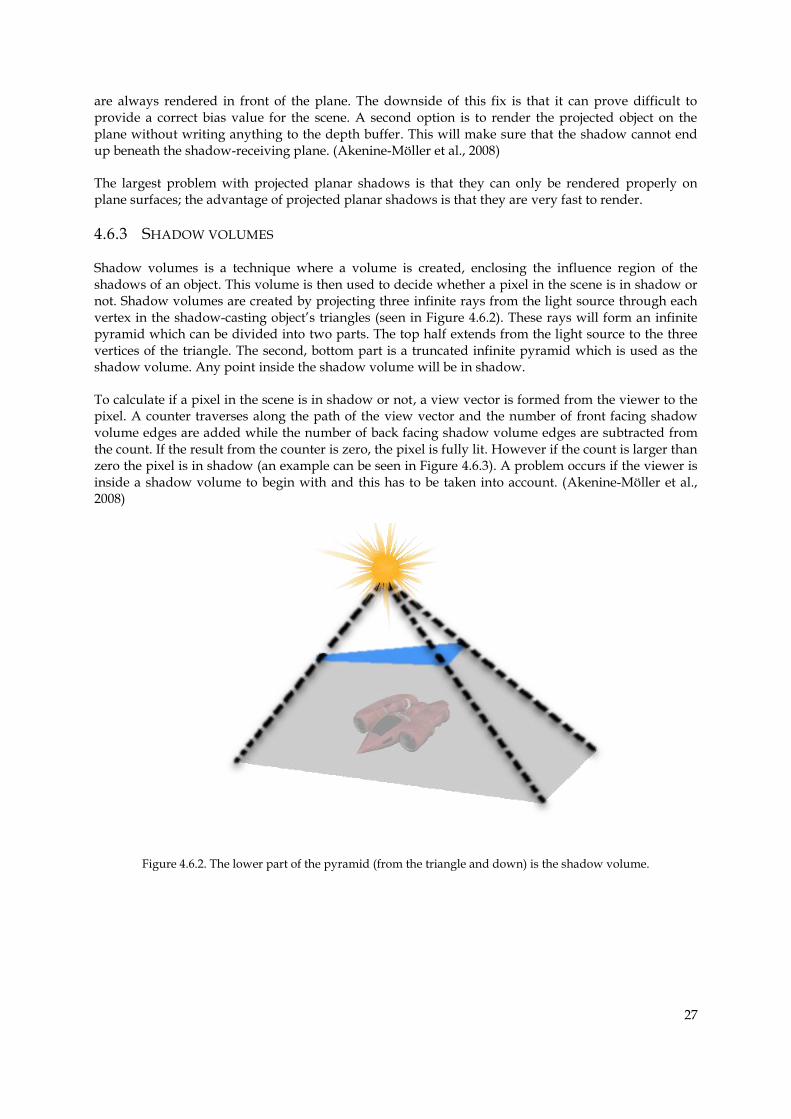
4.6.3 SHADOW VOLUMES

Shadow volumes is a technique where a volume is created, enclosing the influence region of the shadows of an object. This volume is then used to decide whether a pixel in the scene is in shadow or not. Shadow volumes are created by projecting three infinite rays from the light source through each vertex in the shadow-casting object’s triangles (seen in Figure 4.6.2). These rays will form an infinite pyramid which can be divided into two parts. The top half extends from the light source to the three vertices of the triangle. The second, bottom part is a truncated infinite pyramid which is used as the shadow volume. Any point inside the shadow volume will be in shadow.

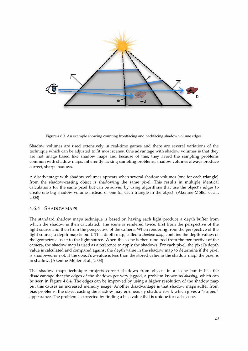
To calculate if a pixel in the scene is in shadow or not, a view vector is formed from the viewer to the pixel. A counter traverses along the path of the view vector and the number of front facing shadow volume edges are added while the number of back facing shadow volume edges are subtracted from the count. If the result from the counter is zero, the pixel is fully lit. However if the count is larger than zero the pixel is in shadow (an example can be seen in Figure 4.6.3). A problem occurs if the viewer is inside a shadow volume to begin with and this has to be taken into account. (Akenine-Möller et al., 2008)

Figure 4.6.2. The lower part of the pyramid (from the triangle and down) is the shadow volume.

28

Figure 4.6.3. An example showing counting frontfacing and backfacing shadow volume edges.

Shadow volumes are used extensively in real-time games and there are several variations of the technique which can be adjusted to fit most scenes. One advantage with shadow volumes is that they are not image based like shadow maps and because of this, they avoid the sampling problems common with shadow maps. Inherently lacking sampling problems, shadow volumes always produce correct, sharp shadows.

A disadvantage with shadow volumes appears when several shadow volumes (one for each triangle) from the shadow-casting object is shadowing the same pixel. This results in multiple identical calculations for the same pixel but can be solved by using algorithms that use the object’s edges to create one big shadow volume instead of one for each triangle in the object. (Akenine-Möller et al., 2008)

4.6.4 SHADOW MAPS

The standard shadow maps technique is based on having each light produce a depth buffer from which the shadow is then calculated. The scene is rendered twice: first from the perspective of the light source and then from the perspective of the camera. When rendering from the perspective of the light source, a depth map is built. This depth map, called a shadow map, contains the depth values of the geometry closest to the light source. When the scene is then rendered from the perspective of the camera, the shadow map is used as a reference to apply the shadows. For each pixel, the pixel’s depth value is calculated and compared against the depth value in the shadow map to determine if the pixel is shadowed or not. If the object’s z-value is less than the stored value in the shadow map, the pixel is in shadow. (Akenine-Möller et al., 2008)

The shadow maps technique projects correct shadows from objects in a scene but it has the disadvantage that the edges of the shadows get very jagged, a problem known as aliasing, which can be seen in Figure 4.6.4. The edges can be improved by using a higher resolution of the shadow map but this causes an increased memory usage. Another disadvantage is that shadow maps suffer from bias problems: the object casting the shadow may erroneously shadow itself, which gives a “striped” appearance. The problem is corrected by finding a bias value that is unique for each scene.

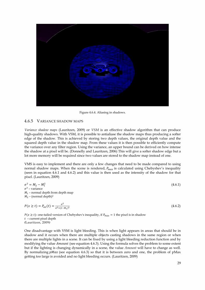
29

Figure 4.6.4. Aliasing in shadows.

4.6.5 VARIANCE SHADOW MAPS

Variance shadow maps (Lauritzen, 2009) or VSM is an effective shadow algorithm that can produce high-quality shadows. With VSM, it is possible to antialiase the shadow maps thus producing a softer edge of the shadow. This is achieved by storing two depth values, the original depth value and the squared depth value in the shadow map. From these values it is then possible to efficiently compute the variance over any filter region. Using the variance, an upper bound can be derived on how intense the shadow at a pixel will be. (Donnelly and Lauritzen, 2006) This will give a softer shadow edge but a lot more memory will be required since two values are stored to the shadow map instead of one.

VMS is easy to implement and there are only a few changes that need to be made compared to using normal shadow maps. When the scene is rendered, is calculated using Chebyshev’s inequality (seen in equation 4.6.1 and 4.6.2) and this value is then used as the intensity of the shadow for that pixel. (Lauritzen, 2009)

(4.6.1)

– variance – normal depth from depth map – (normal depth)2

(4.6.2)

- one-tailed version of Chebyshev's inequality, if the pixel is in shadow – current pixel depth (Lauritzen, 2009)

One disadvantage with VSM is light bleeding. This is when light appears in areas that should be in shadow and it occurs when there are multiple objects casting shadows in the same region or when there are multiple lights in a scene. It can be fixed by using a light bleeding reduction function and by modifying the value (see equation 4.6.3). Using the formula solves the problem to some extent but if the lighting is changing dynamically in a scene, the value Amount will have to change as well. By normalizing (see equation 4.6.3) so that it is between zero and one, the problem of pMax getting too large is avoided and no light bleeding occurs. (Lauritzen, 2009)

30

(4.6.3)

pMax – the amount of shadow at the current pixel clamp(min, max) – a function for making sure that a value stays between min and max Amount – a constant which is changed depending on the scene

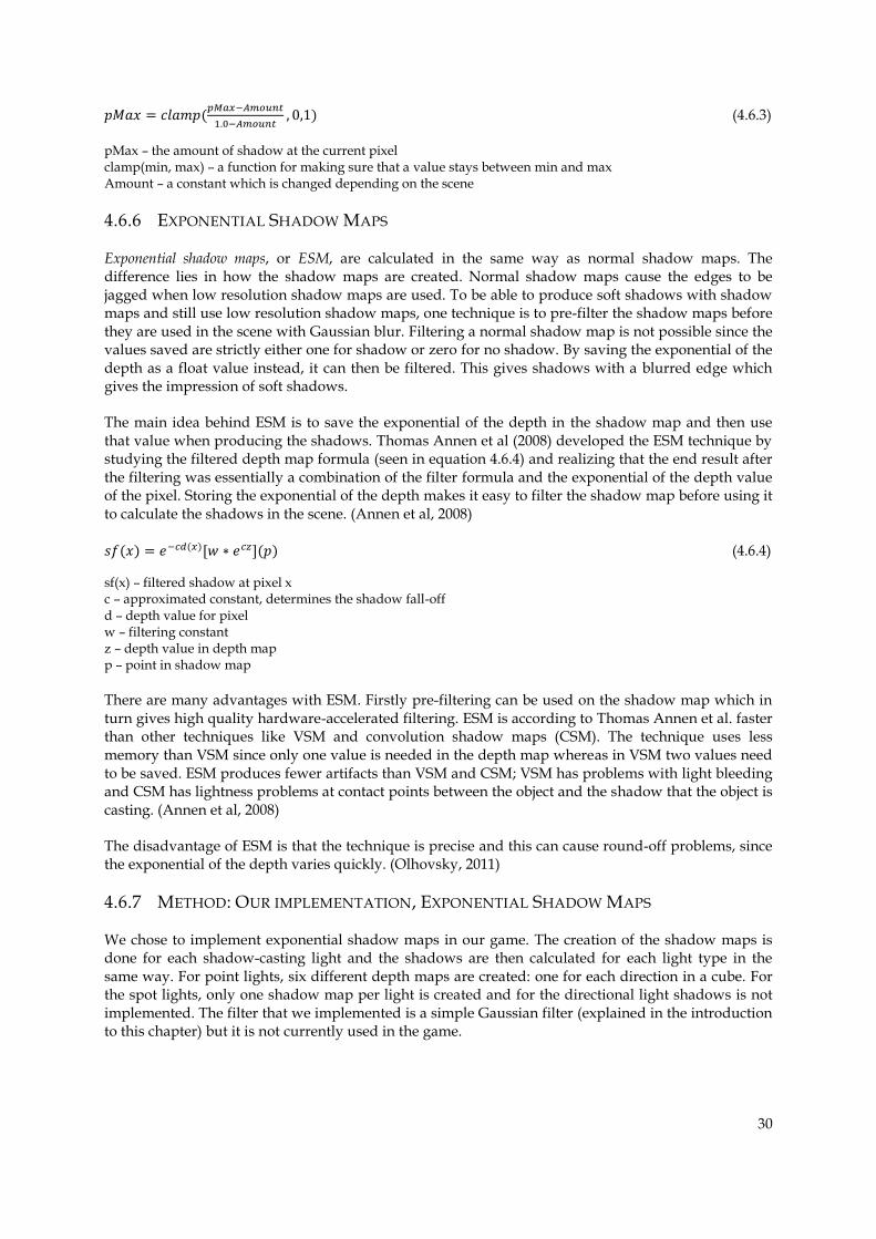
4.6.6 EXPONENTIAL SHADOW MAPS

Exponential shadow maps, or ESM, are calculated in the same way as normal shadow maps. The difference lies in how the shadow maps are created. Normal shadow maps cause the edges to be jagged when low resolution shadow maps are used. To be able to produce soft shadows with shadow maps and still use low resolution shadow maps, one technique is to pre-filter the shadow maps before they are used in the scene with Gaussian blur. Filtering a normal shadow map is not possible since the values saved are strictly either one for shadow or zero for no shadow. By saving the exponential of the depth as a float value instead, it can then be filtered. This gives shadows with a blurred edge which gives the impression of soft shadows.

The main idea behind ESM is to save the exponential of the depth in the shadow map and then use that value when producing the shadows. Thomas Annen et al (2008) developed the ESM technique by studying the filtered depth map formula (seen in equation 4.6.4) and realizing that the end result after the filtering was essentially a combination of the filter formula and the exponential of the depth value of the pixel. Storing the exponential of the depth makes it easy to filter the shadow map before using it to calculate the shadows in the scene. (Annen et al, 2008)

(4.6.4)

sf(x) – filtered shadow at pixel x c – approximated constant, determines the shadow fall-off d – depth value for pixel w – filtering constant z – depth value in depth map p – point in shadow map

There are many advantages with ESM. Firstly pre-filtering can be used on the shadow map which in turn gives high quality hardware-accelerated filtering. ESM is according to Thomas Annen et al. faster than other techniques like VSM and convolution shadow maps (CSM). The technique uses less memory than VSM since only one value is needed in the depth map whereas in VSM two values need to be saved. ESM produces fewer artifacts than VSM and CSM; VSM has problems with light bleeding and CSM has lightness problems at contact points between the object and the shadow that the object is casting. (Annen et al, 2008)

The disadvantage of ESM is that the technique is precise and this can cause round-off problems, since the exponential of the depth varies quickly. (Olhovsky, 2011)

4.6.7 METHOD: OUR IMPLEMENTATION, EXPONENTIAL SHADOW MAPS

We chose to implement exponential shadow maps in our game. The creation of the shadow maps is done for each shadow-casting light and the shadows are then calculated for each light type in the same way. For point lights, six different depth maps are created: one for each direction in a cube. For the spot lights, only one shadow map per light is created and for the directional light shadows is not implemented. The filter that we implemented is a simple Gaussian filter (explained in the introduction to this chapter) but it is not currently used in the game.

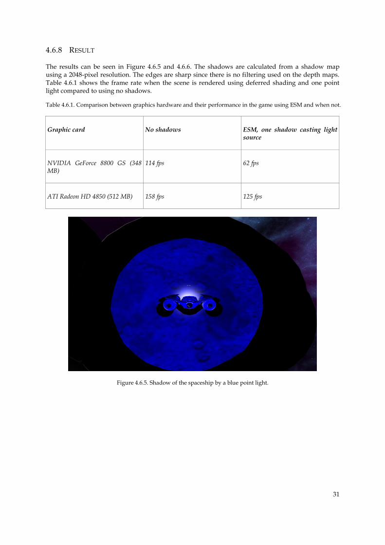
31

4.6.8 RESULT

The results can be seen in Figure 4.6.5 and 4.6.6. The shadows are calculated from a shadow map using a 2048-pixel resolution. The edges are sharp since there is no filtering used on the depth maps. Table 4.6.1 shows the frame rate when the scene is rendered using deferred shading and one point light compared to using no shadows.

Table 4.6.1. Comparison between graphics hardware and their performance in the game using ESM and when not.

Graphic card No shadows ESM, one shadow casting light source

NVIDIA GeForce 8800 GS (348 MB)

114 fps 62 fps

ATI Radeon HD 4850 (512 MB) 158 fps 125 fps

Figure 4.6.5. Shadow of the spaceship by a blue point light.

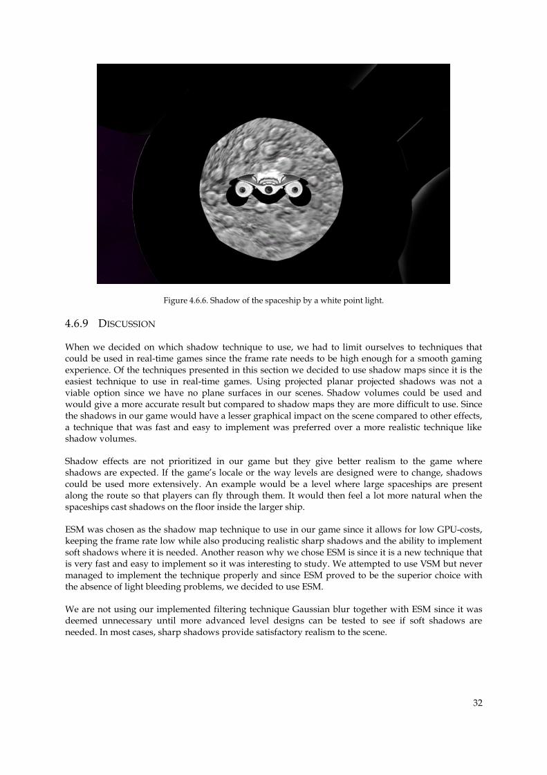
32

Figure 4.6.6. Shadow of the spaceship by a white point light.

4.6.9 DISCUSSION

When we decided on which shadow technique to use, we had to limit ourselves to techniques that could be used in real-time games since the frame rate needs to be high enough for a smooth gaming experience. Of the techniques presented in this section we decided to use shadow maps since it is the easiest technique to use in real-time games. Using projected planar projected shadows was not a viable option since we have no plane surfaces in our scenes. Shadow volumes could be used and would give a more accurate result but compared to shadow maps they are more difficult to use. Since the shadows in our game would have a lesser graphical impact on the scene compared to other effects, a technique that was fast and easy to implement was preferred over a more realistic technique like shadow volumes.

Shadow effects are not prioritized in our game but they give better realism to the game where shadows are expected. If the game’s locale or the way levels are designed were to change, shadows could be used more extensively. An example would be a level where large spaceships are present along the route so that players can fly through them. It would then feel a lot more natural when the spaceships cast shadows on the floor inside the larger ship.

ESM was chosen as the shadow map technique to use in our game since it allows for low GPU-costs, keeping the frame rate low while also producing realistic sharp shadows and the ability to implement soft shadows where it is needed. Another reason why we chose ESM is since it is a new technique that is very fast and easy to implement so it was interesting to study. We attempted to use VSM but never managed to implement the technique properly and since ESM proved to be the superior choice with the absence of light bleeding problems, we decided to use ESM.

We are not using our implemented filtering technique Gaussian blur together with ESM since it was deemed unnecessary until more advanced level designs can be tested to see if soft shadows are needed. In most cases, sharp shadows provide satisfactory realism to the scene.

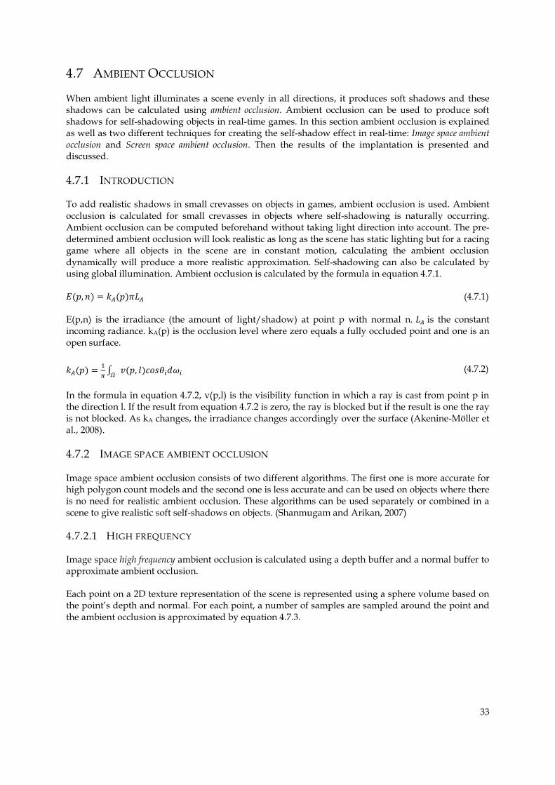
33

4.7 AMBIENT OCCLUSION

When ambient light illuminates a scene evenly in all directions, it produces soft shadows and these shadows can be calculated using ambient occlusion. Ambient occlusion can be used to produce soft shadows for self-shadowing objects in real-time games. In this section ambient occlusion is explained as well as two different techniques for creating the self-shadow effect in real-time: Image space ambient occlusion and Screen space ambient occlusion. Then the results of the implantation is presented and discussed.

4.7.1 INTRODUCTION

To add realistic shadows in small crevasses on objects in games, ambient occlusion is used. Ambient occlusion is calculated for small crevasses in objects where self-shadowing is naturally occurring. Ambient occlusion can be computed beforehand without taking light direction into account. The pre-determined ambient occlusion will look realistic as long as the scene has static lighting but for a racing game where all objects in the scene are in constant motion, calculating the ambient occlusion dynamically will produce a more realistic approximation. Self-shadowing can also be calculated by using global illumination. Ambient occlusion is calculated by the formula in equation 4.7.1.

(4.7.1)

E(p,n) is the irradiance (the amount of light/shadow) at point p with normal n. is the constant incoming radiance. kA(p) is the occlusion level where zero equals a fully occluded point and one is an open surface.

∫

(4.7.2)

In the formula in equation 4.7.2, v(p,l) is the visibility function in which a ray is cast from point p in the direction l. If the result from equation 4.7.2 is zero, the ray is blocked but if the result is one the ray is not blocked. As kA changes, the irradiance changes accordingly over the surface (Akenine-Möller et al., 2008).

4.7.2 IMAGE SPACE AMBIENT OCCLUSION

Image space ambient occlusion consists of two different algorithms. The first one is more accurate for high polygon count models and the second one is less accurate and can be used on objects where there is no need for realistic ambient occlusion. These algorithms can be used separately or combined in a scene to give realistic soft self-shadows on objects. (Shanmugam and Arikan, 2007)

4.7.2.1 HIGH FREQUENCY

Image space high frequency ambient occlusion is calculated using a depth buffer and a normal buffer to approximate ambient occlusion.

Each point on a 2D texture representation of the scene is represented using a sphere volume based on the point’s depth and normal. For each point, a number of samples are sampled around the point and the ambient occlusion is approximated by equation 4.7.3.

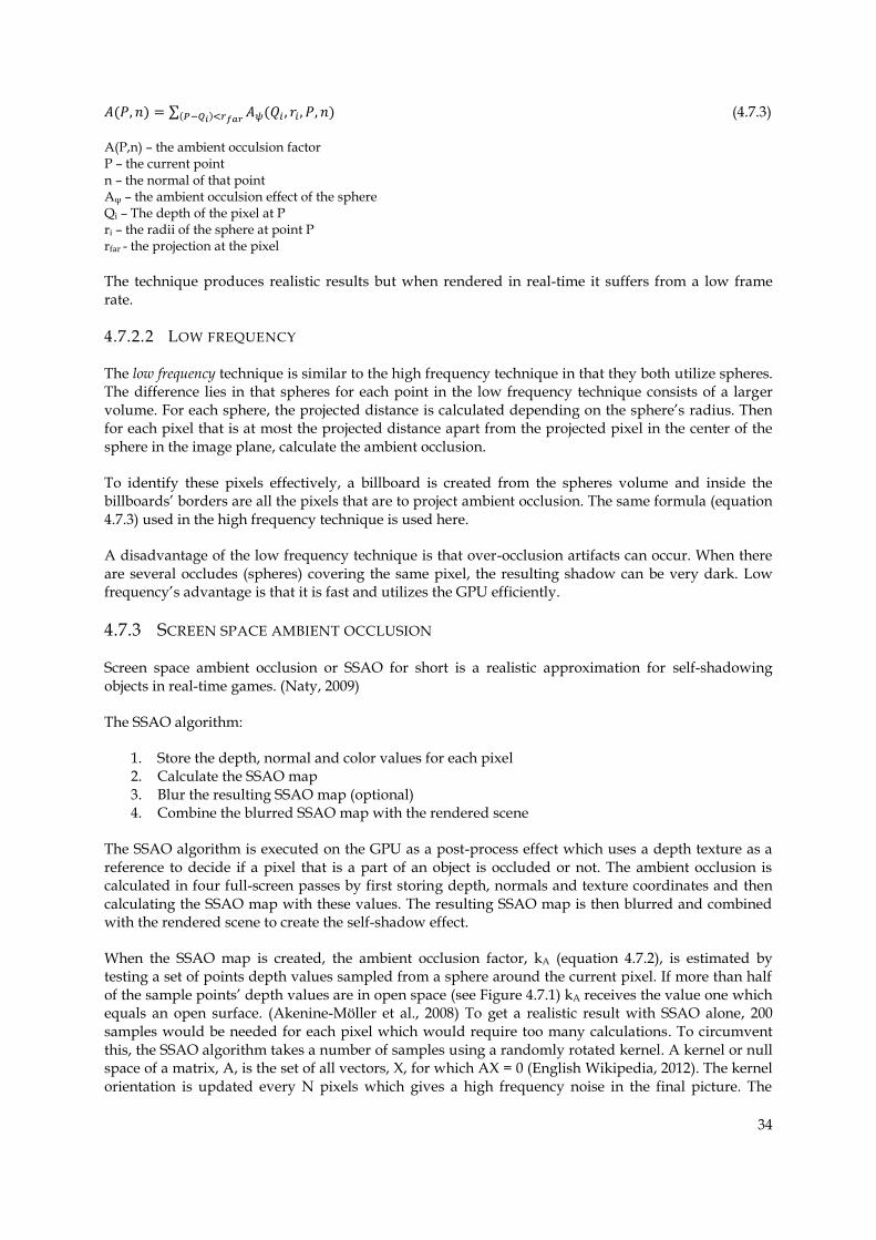
34

∑ (4.7.3)

A(P,n) – the ambient occulsion factor P – the current point n – the normal of that point Aψ – the ambient occulsion effect of the sphere Qi – The depth of the pixel at P ri – the radii of the sphere at point P rfar - the projection at the pixel

The technique produces realistic results but when rendered in real-time it suffers from a low frame rate.

4.7.2.2 LOW FREQUENCY

The low frequency technique is similar to the high frequency technique in that they both utilize spheres. The difference lies in that spheres for each point in the low frequency technique consists of a larger volume. For each sphere, the projected distance is calculated depending on the sphere’s radius. Then for each pixel that is at most the projected distance apart from the projected pixel in the center of the sphere in the image plane, calculate the ambient occlusion.

To identify these pixels effectively, a billboard is created from the spheres volume and inside the billboards’ borders are all the pixels that are to project ambient occlusion. The same formula (equation 4.7.3) used in the high frequency technique is used here.

A disadvantage of the low frequency technique is that over-occlusion artifacts can occur. When there are several occludes (spheres) covering the same pixel, the resulting shadow can be very dark. Low frequency’s advantage is that it is fast and utilizes the GPU efficiently.

4.7.3 SCREEN SPACE AMBIENT OCCLUSION

Screen space ambient occlusion or SSAO for short is a realistic approximation for self-shadowing objects in real-time games. (Naty, 2009)

The SSAO algorithm:

1. Store the depth, normal and color values for each pixel 2. Calculate the SSAO map 3. Blur the resulting SSAO map (optional) 4. Combine the blurred SSAO map with the rendered scene

The SSAO algorithm is executed on the GPU as a post-process effect which uses a depth texture as a reference to decide if a pixel that is a part of an object is occluded or not. The ambient occlusion is calculated in four full-screen passes by first storing depth, normals and texture coordinates and then calculating the SSAO map with these values. The resulting SSAO map is then blurred and combined with the rendered scene to create the self-shadow effect.

When the SSAO map is created, the ambient occlusion factor, kA (equation 4.7.2), is estimated by testing a set of points depth values sampled from a sphere around the current pixel. If more than half of the sample points’ depth values are in open space (see Figure 4.7.1) kA receives the value one which equals an open surface. (Akenine-Möller et al., 2008) To get a realistic result with SSAO alone, 200 samples would be needed for each pixel which would require too many calculations. To circumvent this, the SSAO algorithm takes a number of samples using a randomly rotated kernel. A kernel or null space of a matrix, A, is the set of all vectors, X, for which AX = 0 (English Wikipedia, 2012). The kernel orientation is updated every N pixels which gives a high frequency noise in the final picture. The

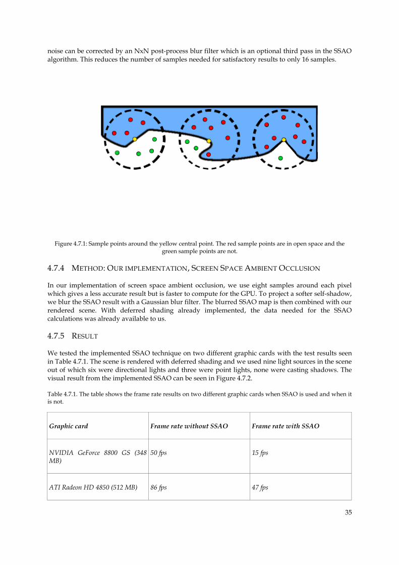
35

noise can be corrected by an NxN post-process blur filter which is an optional third pass in the SSAO algorithm. This reduces the number of samples needed for satisfactory results to only 16 samples.

Figure 4.7.1: Sample points around the yellow central point. The red sample points are in open space and the green sample points are not.

4.7.4 METHOD: OUR IMPLEMENTATION, SCREEN SPACE AMBIENT OCCLUSION

In our implementation of screen space ambient occlusion, we use eight samples around each pixel which gives a less accurate result but is faster to compute for the GPU. To project a softer self-shadow, we blur the SSAO result with a Gaussian blur filter. The blurred SSAO map is then combined with our rendered scene. With deferred shading already implemented, the data needed for the SSAO calculations was already available to us.

4.7.5 RESULT

We tested the implemented SSAO technique on two different graphic cards with the test results seen in Table 4.7.1. The scene is rendered with deferred shading and we used nine light sources in the scene out of which six were directional lights and three were point lights, none were casting shadows. The visual result from the implemented SSAO can be seen in Figure 4.7.2.

Table 4.7.1. The table shows the frame rate results on two different graphic cards when SSAO is used and when it is not.

Graphic card Frame rate without SSAO Frame rate with SSAO

NVIDIA GeForce 8800 GS (348 MB)

50 fps 15 fps

ATI Radeon HD 4850 (512 MB) 86 fps 47 fps

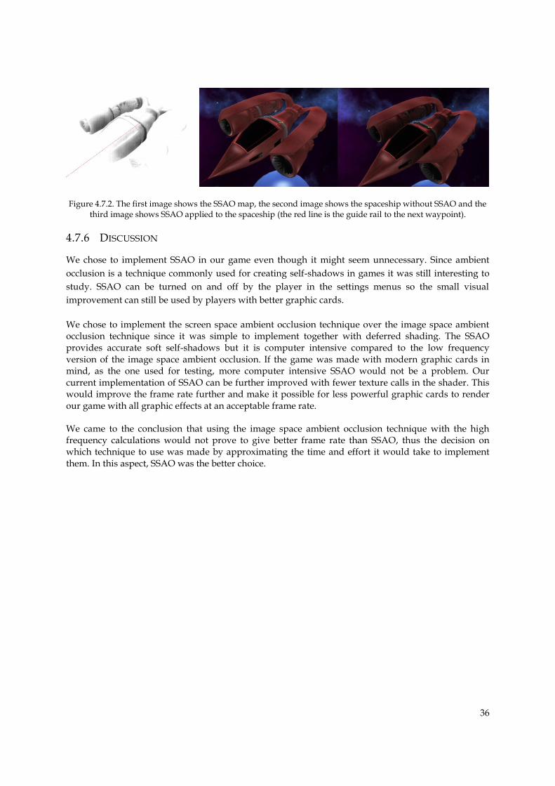
36

Figure 4.7.2. The first image shows the SSAO map, the second image shows the spaceship without SSAO and the third image shows SSAO applied to the spaceship (the red line is the guide rail to the next waypoint).

4.7.6 DISCUSSION

We chose to implement SSAO in our game even though it might seem unnecessary. Since ambient

occlusion is a technique commonly used for creating self-shadows in games it was still interesting to

study. SSAO can be turned on and off by the player in the settings menus so the small visual

improvement can still be used by players with better graphic cards.

We chose to implement the screen space ambient occlusion technique over the image space ambient occlusion technique since it was simple to implement together with deferred shading. The SSAO provides accurate soft self-shadows but it is computer intensive compared to the low frequency version of the image space ambient occlusion. If the game was made with modern graphic cards in mind, as the one used for testing, more computer intensive SSAO would not be a problem. Our current implementation of SSAO can be further improved with fewer texture calls in the shader. This would improve the frame rate further and make it possible for less powerful graphic cards to render our game with all graphic effects at an acceptable frame rate.

We came to the conclusion that using the image space ambient occlusion technique with the high frequency calculations would not prove to give better frame rate than SSAO, thus the decision on which technique to use was made by approximating the time and effort it would take to implement them. In this aspect, SSAO was the better choice.

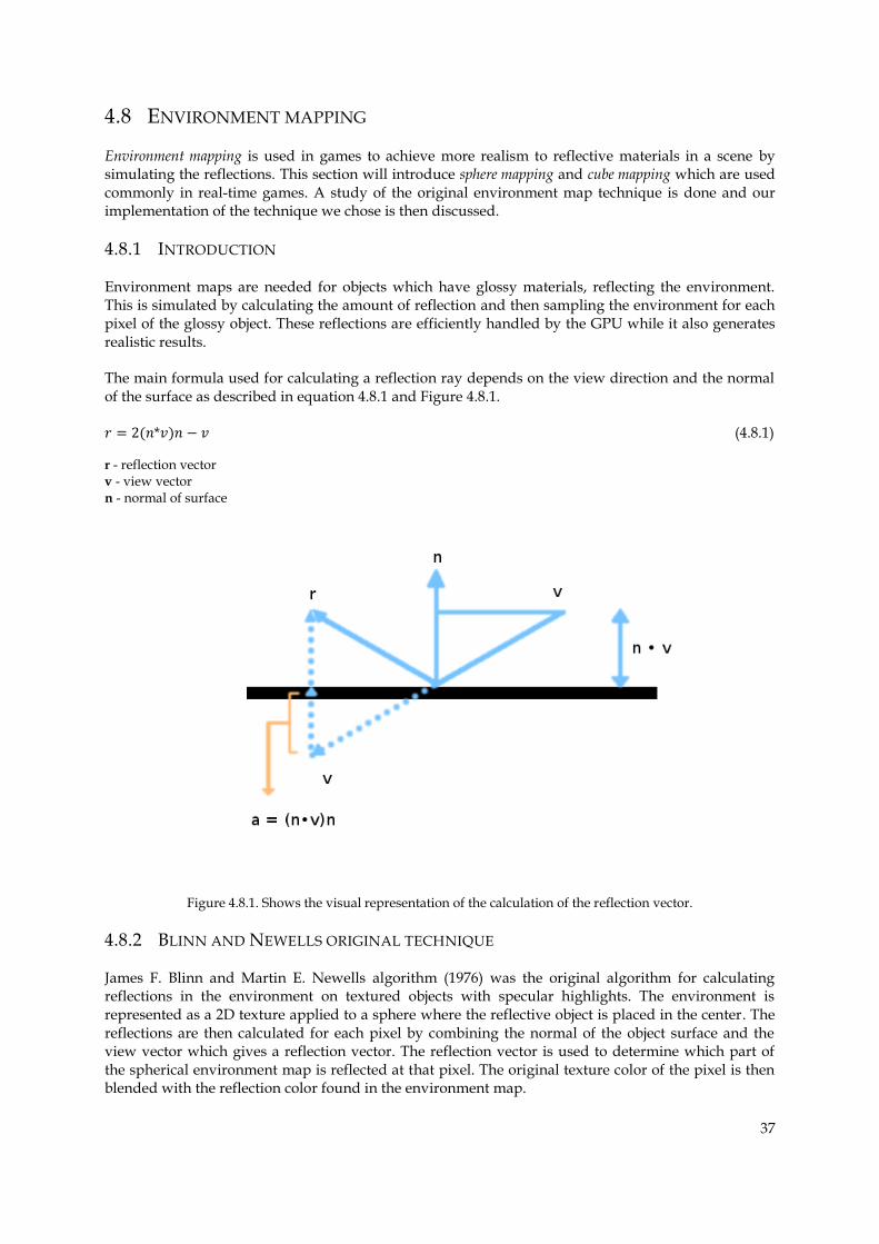
37

4.8 ENVIRONMENT MAPPING

Environment mapping is used in games to achieve more realism to reflective materials in a scene by simulating the reflections. This section will introduce sphere mapping and cube mapping which are used commonly in real-time games. A study of the original environment map technique is done and our implementation of the technique we chose is then discussed.

4.8.1 INTRODUCTION

Environment maps are needed for objects which have glossy materials, reflecting the environment. This is simulated by calculating the amount of reflection and then sampling the environment for each pixel of the glossy object. These reflections are efficiently handled by the GPU while it also generates realistic results.

The main formula used for calculating a reflection ray depends on the view direction and the normal of the surface as described in equation 4.8.1 and Figure 4.8.1.

(4.8.1)

r - reflection vector v - view vector n - normal of surface

Figure 4.8.1. Shows the visual representation of the calculation of the reflection vector.

4.8.2 BLINN AND NEWELLS ORIGINAL TECHNIQUE

James F. Blinn and Martin E. Newells algorithm (1976) was the original algorithm for calculating reflections in the environment on textured objects with specular highlights. The environment is represented as a 2D texture applied to a sphere where the reflective object is placed in the center. The reflections are then calculated for each pixel by combining the normal of the object surface and the view vector which gives a reflection vector. The reflection vector is used to determine which part of the spherical environment map is reflected at that pixel. The original texture color of the pixel is then blended with the reflection color found in the environment map.

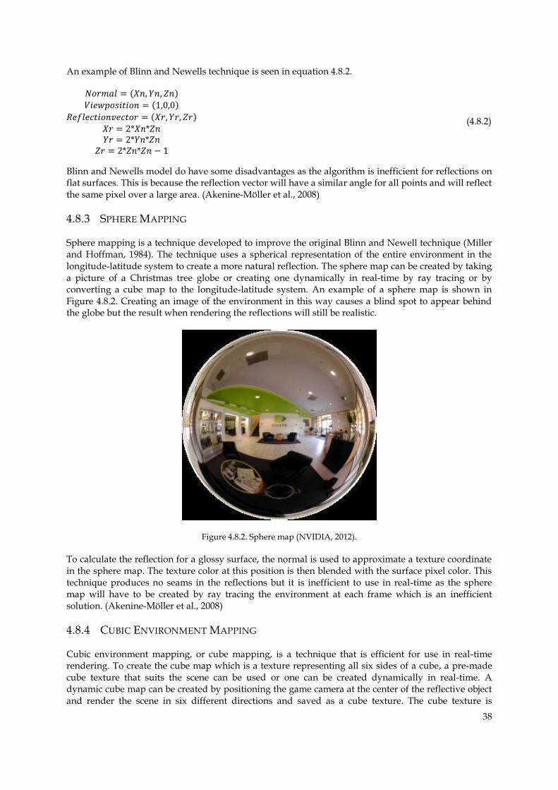
38

An example of Blinn and Newells technique is seen in equation 4.8.2.

(4.8.2)

Blinn and Newells model do have some disadvantages as the algorithm is inefficient for reflections on flat surfaces. This is because the reflection vector will have a similar angle for all points and will reflect the same pixel over a large area. (Akenine-Möller et al., 2008)

4.8.3 SPHERE MAPPING

Sphere mapping is a technique developed to improve the original Blinn and Newell technique (Miller and Hoffman, 1984). The technique uses a spherical representation of the entire environment in the longitude-latitude system to create a more natural reflection. The sphere map can be created by taking a picture of a Christmas tree globe or creating one dynamically in real-time by ray tracing or by converting a cube map to the longitude-latitude system. An example of a sphere map is shown in Figure 4.8.2. Creating an image of the environment in this way causes a blind spot to appear behind the globe but the result when rendering the reflections will still be realistic.

Figure 4.8.2. Sphere map (NVIDIA, 2012).

To calculate the reflection for a glossy surface, the normal is used to approximate a texture coordinate in the sphere map. The texture color at this position is then blended with the surface pixel color. This technique produces no seams in the reflections but it is inefficient to use in real-time as the sphere map will have to be created by ray tracing the environment at each frame which is an inefficient solution. (Akenine-Möller et al., 2008)

4.8.4 CUBIC ENVIRONMENT MAPPING

Cubic environment mapping, or cube mapping, is a technique that is efficient for use in real-time rendering. To create the cube map which is a texture representing all six sides of a cube, a pre-made cube texture that suits the scene can be used or one can be created dynamically in real-time. A dynamic cube map can be created by positioning the game camera at the center of the reflective object and render the scene in six different directions and saved as a cube texture. The cube texture is

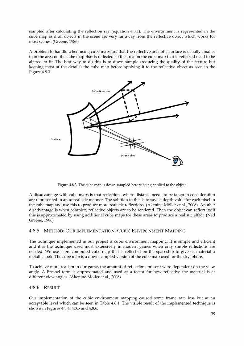
39

sampled after calculating the reflection ray (equation 4.8.1). The environment is represented in the cube map as if all objects in the scene are very far away from the reflective object which works for most scenes. (Greene, 1986)

A problem to handle when using cube maps are that the reflective area of a surface is usually smaller than the area on the cube map that is reflected so the area on the cube map that is reflected need to be altered to fit. The best way to do this is to down sample (reducing the quality of the texture but keeping most of the details) the cube map before applying it to the reflective object as seen in the Figure 4.8.3.

Figure 4.8.3. The cube map is down sampled before being applied to the object.

A disadvantage with cube maps is that reflections where distance needs to be taken in consideration are represented in an unrealistic manner. The solution to this is to save a depth value for each pixel in the cube map and use this to produce more realistic reflections. (Akenine-Möller et al., 2008) Another disadvantage is when complex, reflective objects are to be rendered. Then the object can reflect itself this is approximated by using additional cube maps for these areas to produce a realistic effect. (Ned Greene, 1986)

4.8.5 METHOD: OUR IMPLEMENTATION, CUBIC ENVIRONMENT MAPPING

The technique implemented in our project is cubic environment mapping. It is simple and efficient and it is the technique used most extensively in modern games when only simple reflections are needed. We use a pre-computed cube map that is reflected on the spaceship to give its material a metallic look. The cube map is a down sampled version of the cube map used for the skysphere.

To achieve more realism in our game, the amount of reflections present were dependent on the view angle. A Fresnel term is approximated and used as a factor for how reflective the material is at different view angles. (Akenine-Möller et al., 2008)

4.8.6 RESULT

Our implementation of the cubic environment mapping caused some frame rate loss but at an acceptable level which can be seen in Table 4.8.1. The visible result of the implemented technique is shown in Figures 4.8.4, 4.8.5 and 4.8.6.

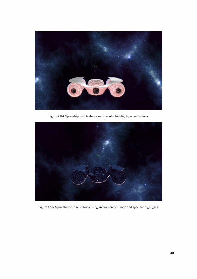
40

Figure 4.8.4. Spaceship with textures and specular highlights, no reflections.

Figure 4.8.5. Spaceship with reflections using an environment map and specular highlights.

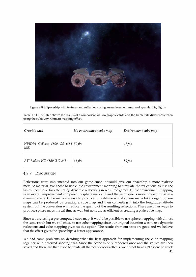
41

Figure 4.8.6. Spaceship with textures and reflections using an environment map and specular highlights.

Table 4.8.1. The table shows the results of a comparison of two graphic cards and the frame rate differences when using the cubic environment mapping effect.

Graphic card No environment cube map Environment cube map

NVIDIA GeForce 8800 GS (384 MB)

50 fps 47 fps

ATI Radeon HD 4850 (512 MB) 86 fps 80 fps

4.8.7 DISCUSSION

Reflections were implemented into our game since it would give our spaceship a more realistic metallic material. We chose to use cubic environment mapping to simulate the reflections as it is the fastest technique for calculating dynamic reflections in real-time games. Cubic environment mapping is an overall improvement compared to sphere mapping and the technique is more proper to use in a dynamic scene. Cube maps are easy to produce in real-time whilst sphere maps take longer. Sphere maps can be produced by creating a cube map and then converting it into the longitude-latitude system but the conversion will reduce the quality of the resulting reflections. There are other ways to produce sphere maps in real-time as well but none are as efficient as creating a plain cube map.

Since we are using a pre-computed cube map, it would be possible to use sphere mapping with almost the same result but we still chose to use cube mapping since our original intention was to use dynamic reflections and cube mapping gives us this option. The results from our tests are good and we believe that the effect gives the spaceships a better appearance.

We had some problems on deciding what the best approach for implementing the cube mapping together with deferred shading was. Since the scene is only rendered once and the values are then saved and these are then used to create all the post-process effects, we do not have a 3D scene to work

42

with when calculating the reflections. We chose to use a pre-computed cube map for simplicity. To decide which parts of the scene was to receive reflections we used the specularity values to identify the spaceships in the scene. This made it possible to allow for only the spaceship to be reflective.

Future improvements of the cube mapping effect would be to implement dynamic cube mapping. There exists techniques for computing dynamic reflections for deferred shading but since there was a limited amount of information about the techniques available, it was determined to be too time consuming to implement.

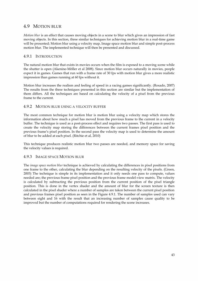
43

4.9 MOTION BLUR

Motion blur is an effect that causes moving objects in a scene to blur which gives an impression of fast moving objects. In this section, three similar techniques for achieving motion blur in a real-time game will be presented; Motion blur using a velocity map, Image space motion blur and simple post-process motion blur. The implemented technique will then be presented and discussed.

4.9.1 INTRODUCTION

The natural motion blur that exists in movies occurs when the film is exposed to a moving scene while the shutter is open (Akenine-Möller et al 2008). Since motion blur occurs naturally in movies, people expect it in games. Games that run with a frame rate of 30 fps with motion blur gives a more realistic impression than games running at 60 fps without it.

Motion blur increases the realism and feeling of speed in a racing games significantly. (Rosado, 2007) The results from the three techniques presented in this section are similar but the implementation of them differs. All the techniques are based on calculating the velocity of a pixel from the previous frame to the current.

4.9.2 MOTION BLUR USING A VELOCITY BUFFER

The most common technique for motion blur is motion blur using a velocity map which stores the information about how much a pixel has moved from the previous frame to the current in a velocity buffer. The technique is used as a post-process effect and requires two passes. The first pass is used to create the velocity map storing the differences between the current frames pixel position and the previous frame’s pixel position. In the second pass the velocity map is used to determine the amount of blur to be added at each pixel. (Ritchie et al, 2010)

This technique produces realistic motion blur two passes are needed, and memory space for saving the velocity values is required.

4.9.3 IMAGE SPACE MOTION BLUR

The image space motion blur technique is achieved by calculating the differences in pixel positions from one frame to the other, calculating the blur depending on the resulting velocity of the pixels. (Green, 2003) The technique is simple in its implementation and it only needs one pass to compute, values needed are; the previous frame pixel position and the previous frame model-view matrix. The velocity is calculated by subtracting the previous position from the current position of the pixel triangle position. This is done in the vertex shader and the amount of blur for the screen texture is then calculated in the pixel shader where a number of samples are taken between the current pixel position and previous frames pixel position as seen in the Figure 4.9.1. The number of samples used can vary between eight and 16 with the result that an increasing number of samples cause quality to be improved but the number of computations required for rendering the scene increases.

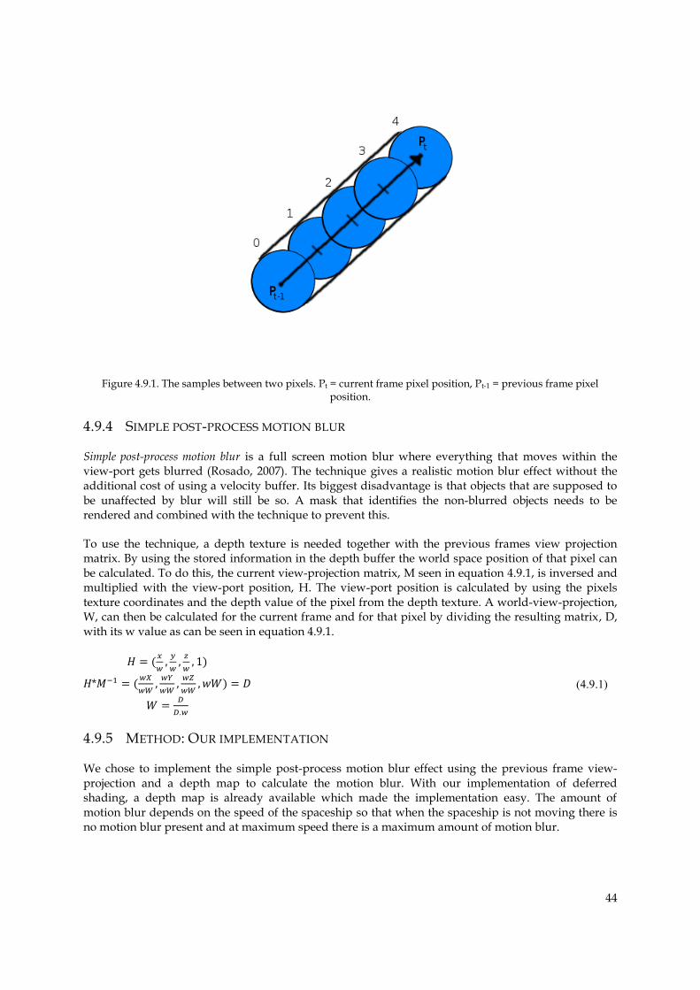
44

Figure 4.9.1. The samples between two pixels. Pt = current frame pixel position, Pt-1 = previous frame pixel position.

4.9.4 SIMPLE POST-PROCESS MOTION BLUR

Simple post-process motion blur is a full screen motion blur where everything that moves within the view-port gets blurred (Rosado, 2007). The technique gives a realistic motion blur effect without the additional cost of using a velocity buffer. Its biggest disadvantage is that objects that are supposed to be unaffected by blur will still be so. A mask that identifies the non-blurred objects needs to be rendered and combined with the technique to prevent this.

To use the technique, a depth texture is needed together with the previous frames view projection matrix. By using the stored information in the depth buffer the world space position of that pixel can be calculated. To do this, the current view-projection matrix, M seen in equation 4.9.1, is inversed and multiplied with the view-port position, H. The view-port position is calculated by using the pixels texture coordinates and the depth value of the pixel from the depth texture. A world-view-projection, W, can then be calculated for the current frame and for that pixel by dividing the resulting matrix, D, with its w value as can be seen in equation 4.9.1.

𝑤 𝑦

𝑤

𝑤

𝑤𝑋

𝑤𝑊

𝑤𝑌

𝑤𝑊

𝑤𝑍

𝑤𝑊 𝐷

𝐷

𝐷.𝑤

(4.9.1)

4.9.5 METHOD: OUR IMPLEMENTATION

We chose to implement the simple post-process motion blur effect using the previous frame view-projection and a depth map to calculate the motion blur. With our implementation of deferred shading, a depth map is already available which made the implementation easy. The amount of motion blur depends on the speed of the spaceship so that when the spaceship is not moving there is no motion blur present and at maximum speed there is a maximum amount of motion blur.

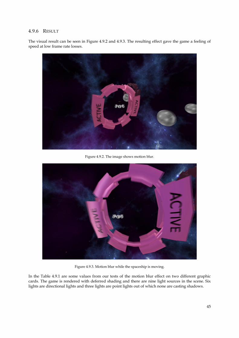
45

4.9.6 RESULT

The visual result can be seen in Figure 4.9.2 and 4.9.3. The resulting effect gave the game a feeling of speed at low frame rate losses.

Figure 4.9.2. The image shows motion blur.

Figure 4.9.3. Motion blur while the spaceship is moving.

In the Table 4.9.1 are some values from our tests of the motion blur effect on two different graphic cards. The game is rendered with deferred shading and there are nine light sources in the scene. Six lights are directional lights and three lights are point lights out of which none are casting shadows.

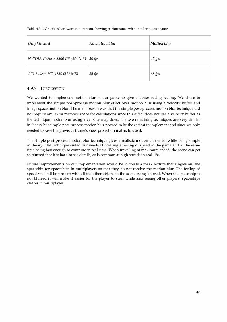
46

Table 4.9.1. Graphics hardware comparison showing performance when rendering our game.

Graphic card No motion blur Motion blur

NVIDIA GeForce 8800 GS (384 MB) 50 fps 47 fps

ATI Radeon HD 4850 (512 MB) 86 fps 68 fps

4.9.7 DISCUSSION

We wanted to implement motion blur in our game to give a better racing feeling. We chose to

implement the simple post-process motion blur effect over motion blur using a velocity buffer and

image space motion blur. The main reason was that the simple post-process motion blur technique did

not require any extra memory space for calculations since this effect does not use a velocity buffer as

the technique motion blur using a velocity map does. The two remaining techniques are very similar

in theory but simple post-process motion blur proved to be the easiest to implement and since we only

needed to save the previous frame’s view projection matrix to use it.

The simple post-process motion blur technique gives a realistic motion blur effect while being simple in theory. The technique suited our needs of creating a feeling of speed in the game and at the same time being fast enough to compute in real-time. When travelling at maximum speed, the scene can get so blurred that it is hard to see details, as is common at high speeds in real-life.

Future improvements on our implementation would be to create a mask texture that singles out the spaceship (or spaceships in multiplayer) so that they do not receive the motion blur. The feeling of speed will still be present with all the other objects in the scene being blurred. When the spaceship is not blurred it will make it easier for the player to steer while also seeing other players’ spaceships clearer in multiplayer.

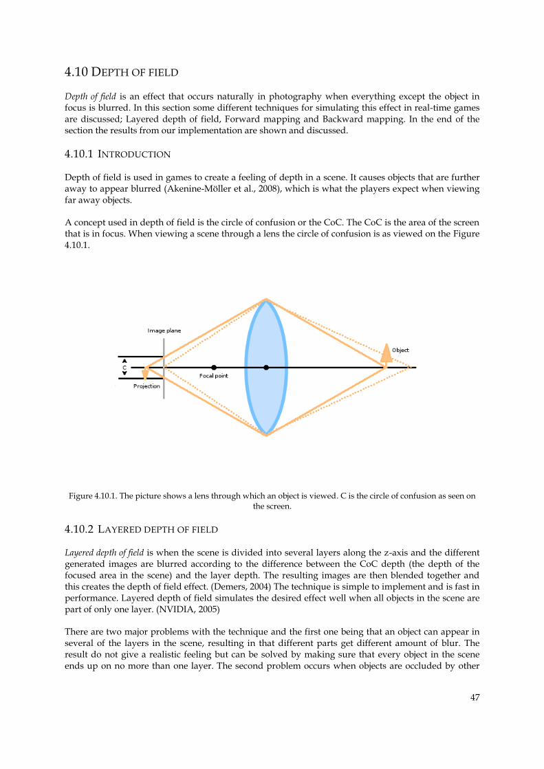
47

4.10 DEPTH OF FIELD

Depth of field is an effect that occurs naturally in photography when everything except the object in focus is blurred. In this section some different techniques for simulating this effect in real-time games are discussed; Layered depth of field, Forward mapping and Backward mapping. In the end of the section the results from our implementation are shown and discussed.

4.10.1 INTRODUCTION

Depth of field is used in games to create a feeling of depth in a scene. It causes objects that are further away to appear blurred (Akenine-Möller et al., 2008), which is what the players expect when viewing far away objects.

A concept used in depth of field is the circle of confusion or the CoC. The CoC is the area of the screen that is in focus. When viewing a scene through a lens the circle of confusion is as viewed on the Figure 4.10.1.

Figure 4.10.1. The picture shows a lens through which an object is viewed. C is the circle of confusion as seen on the screen.

4.10.2 LAYERED DEPTH OF FIELD

Layered depth of field is when the scene is divided into several layers along the z-axis and the different generated images are blurred according to the difference between the CoC depth (the depth of the focused area in the scene) and the layer depth. The resulting images are then blended together and this creates the depth of field effect. (Demers, 2004) The technique is simple to implement and is fast in performance. Layered depth of field simulates the desired effect well when all objects in the scene are part of only one layer. (NVIDIA, 2005)

There are two major problems with the technique and the first one being that an object can appear in several of the layers in the scene, resulting in that different parts get different amount of blur. The result do not give a realistic feeling but can be solved by making sure that every object in the scene ends up on no more than one layer. The second problem occurs when objects are occluded by other

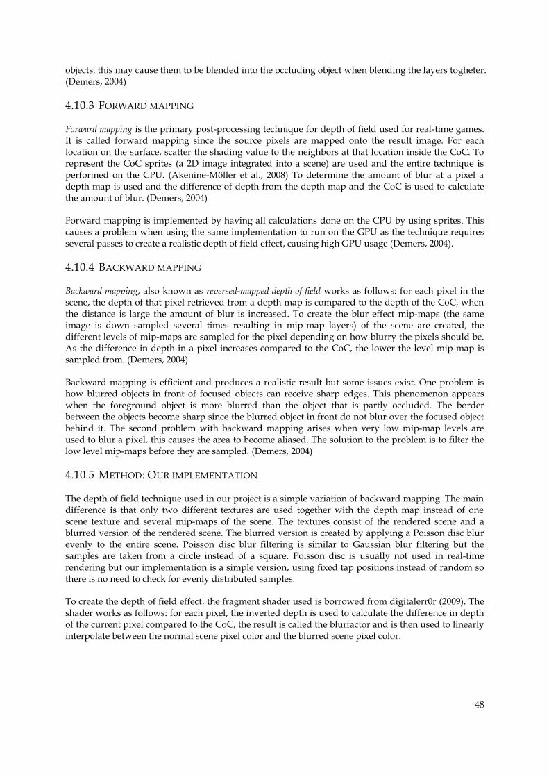
48

objects, this may cause them to be blended into the occluding object when blending the layers togheter. (Demers, 2004)

4.10.3 FORWARD MAPPING

Forward mapping is the primary post-processing technique for depth of field used for real-time games. It is called forward mapping since the source pixels are mapped onto the result image. For each location on the surface, scatter the shading value to the neighbors at that location inside the CoC. To represent the CoC sprites (a 2D image integrated into a scene) are used and the entire technique is performed on the CPU. (Akenine-Möller et al., 2008) To determine the amount of blur at a pixel a depth map is used and the difference of depth from the depth map and the CoC is used to calculate the amount of blur. (Demers, 2004)

Forward mapping is implemented by having all calculations done on the CPU by using sprites. This causes a problem when using the same implementation to run on the GPU as the technique requires several passes to create a realistic depth of field effect, causing high GPU usage (Demers, 2004).

4.10.4 BACKWARD MAPPING

Backward mapping, also known as reversed-mapped depth of field works as follows: for each pixel in the scene, the depth of that pixel retrieved from a depth map is compared to the depth of the CoC, when the distance is large the amount of blur is increased. To create the blur effect mip-maps (the same image is down sampled several times resulting in mip-map layers) of the scene are created, the different levels of mip-maps are sampled for the pixel depending on how blurry the pixels should be. As the difference in depth in a pixel increases compared to the CoC, the lower the level mip-map is sampled from. (Demers, 2004)

Backward mapping is efficient and produces a realistic result but some issues exist. One problem is how blurred objects in front of focused objects can receive sharp edges. This phenomenon appears when the foreground object is more blurred than the object that is partly occluded. The border between the objects become sharp since the blurred object in front do not blur over the focused object behind it. The second problem with backward mapping arises when very low mip-map levels are used to blur a pixel, this causes the area to become aliased. The solution to the problem is to filter the low level mip-maps before they are sampled. (Demers, 2004)

4.10.5 METHOD: OUR IMPLEMENTATION

The depth of field technique used in our project is a simple variation of backward mapping. The main difference is that only two different textures are used together with the depth map instead of one scene texture and several mip-maps of the scene. The textures consist of the rendered scene and a blurred version of the rendered scene. The blurred version is created by applying a Poisson disc blur evenly to the entire scene. Poisson disc blur filtering is similar to Gaussian blur filtering but the samples are taken from a circle instead of a square. Poisson disc is usually not used in real-time rendering but our implementation is a simple version, using fixed tap positions instead of random so there is no need to check for evenly distributed samples.

To create the depth of field effect, the fragment shader used is borrowed from digitalerr0r (2009). The shader works as follows: for each pixel, the inverted depth is used to calculate the difference in depth of the current pixel compared to the CoC, the result is called the blurfactor and is then used to linearly interpolate between the normal scene pixel color and the blurred scene pixel color.

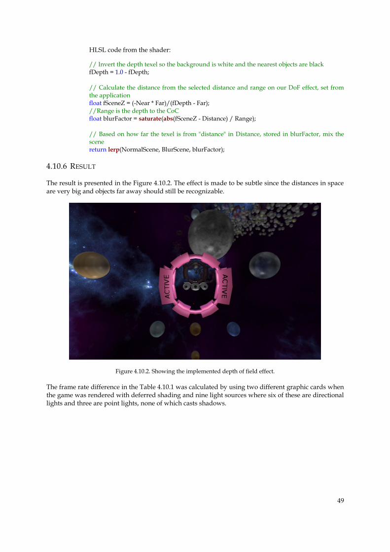
49

HLSL code from the shader:

// Invert the depth texel so the background is white and the nearest objects are black fDepth = 1.0 - fDepth;

// Calculate the distance from the selected distance and range on our DoF effect, set from the application

float fSceneZ = (-Near * Far)/(fDepth - Far); //Range is the depth to the CoC float blurFactor = saturate(abs(fSceneZ - Distance) / Range);

// Based on how far the texel is from "distance" in Distance, stored in blurFactor, mix the scene

return lerp(NormalScene, BlurScene, blurFactor);

4.10.6 RESULT

The result is presented in the Figure 4.10.2. The effect is made to be subtle since the distances in space are very big and objects far away should still be recognizable.

Figure 4.10.2. Showing the implemented depth of field effect.

The frame rate difference in the Table 4.10.1 was calculated by using two different graphic cards when the game was rendered with deferred shading and nine light sources where six of these are directional lights and three are point lights, none of which casts shadows.

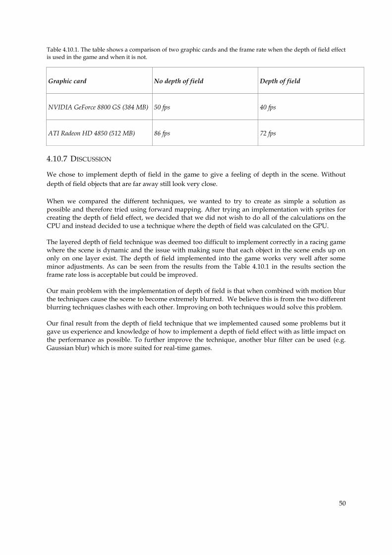
50

Table 4.10.1. The table shows a comparison of two graphic cards and the frame rate when the depth of field effect is used in the game and when it is not.

Graphic card No depth of field Depth of field

NVIDIA GeForce 8800 GS (384 MB) 50 fps 40 fps

ATI Radeon HD 4850 (512 MB) 86 fps 72 fps

4.10.7 DISCUSSION

We chose to implement depth of field in the game to give a feeling of depth in the scene. Without

depth of field objects that are far away still look very close.

When we compared the different techniques, we wanted to try to create as simple a solution as possible and therefore tried using forward mapping. After trying an implementation with sprites for creating the depth of field effect, we decided that we did not wish to do all of the calculations on the CPU and instead decided to use a technique where the depth of field was calculated on the GPU.

The layered depth of field technique was deemed too difficult to implement correctly in a racing game where the scene is dynamic and the issue with making sure that each object in the scene ends up on only on one layer exist. The depth of field implemented into the game works very well after some minor adjustments. As can be seen from the results from the Table 4.10.1 in the results section the frame rate loss is acceptable but could be improved.

Our main problem with the implementation of depth of field is that when combined with motion blur the techniques cause the scene to become extremely blurred. We believe this is from the two different blurring techniques clashes with each other. Improving on both techniques would solve this problem.

Our final result from the depth of field technique that we implemented caused some problems but it gave us experience and knowledge of how to implement a depth of field effect with as little impact on the performance as possible. To further improve the technique, another blur filter can be used (e.g. Gaussian blur) which is more suited for real-time games.

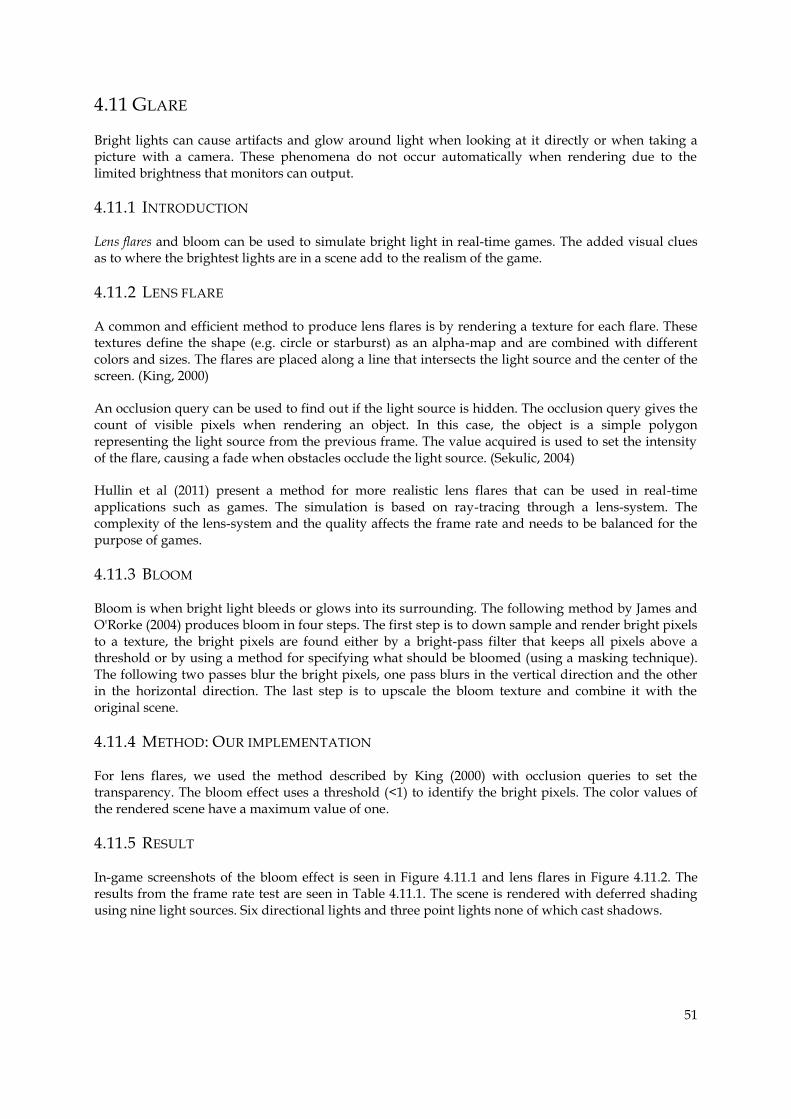
51

4.11 GLARE

Bright lights can cause artifacts and glow around light when looking at it directly or when taking a picture with a camera. These phenomena do not occur automatically when rendering due to the limited brightness that monitors can output.

4.11.1 INTRODUCTION

Lens flares and bloom can be used to simulate bright light in real-time games. The added visual clues as to where the brightest lights are in a scene add to the realism of the game.

4.11.2 LENS FLARE

A common and efficient method to produce lens flares is by rendering a texture for each flare. These textures define the shape (e.g. circle or starburst) as an alpha-map and are combined with different colors and sizes. The flares are placed along a line that intersects the light source and the center of the screen. (King, 2000)

An occlusion query can be used to find out if the light source is hidden. The occlusion query gives the count of visible pixels when rendering an object. In this case, the object is a simple polygon representing the light source from the previous frame. The value acquired is used to set the intensity of the flare, causing a fade when obstacles occlude the light source. (Sekulic, 2004)

Hullin et al (2011) present a method for more realistic lens flares that can be used in real-time applications such as games. The simulation is based on ray-tracing through a lens-system. The complexity of the lens-system and the quality affects the frame rate and needs to be balanced for the purpose of games.

4.11.3 BLOOM

Bloom is when bright light bleeds or glows into its surrounding. The following method by James and O'Rorke (2004) produces bloom in four steps. The first step is to down sample and render bright pixels to a texture, the bright pixels are found either by a bright-pass filter that keeps all pixels above a threshold or by using a method for specifying what should be bloomed (using a masking technique). The following two passes blur the bright pixels, one pass blurs in the vertical direction and the other in the horizontal direction. The last step is to upscale the bloom texture and combine it with the original scene.

4.11.4 METHOD: OUR IMPLEMENTATION

For lens flares, we used the method described by King (2000) with occlusion queries to set the transparency. The bloom effect uses a threshold (<1) to identify the bright pixels. The color values of the rendered scene have a maximum value of one.

4.11.5 RESULT

In-game screenshots of the bloom effect is seen in Figure 4.11.1 and lens flares in Figure 4.11.2. The results from the frame rate test are seen in Table 4.11.1. The scene is rendered with deferred shading using nine light sources. Six directional lights and three point lights none of which cast shadows.

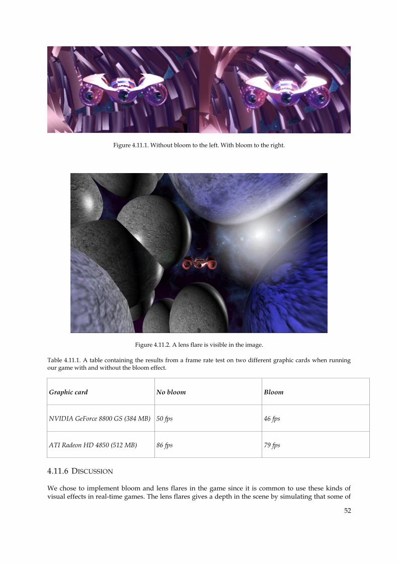
52

Figure 4.11.1. Without bloom to the left. With bloom to the right.

Figure 4.11.2. A lens flare is visible in the image.

Table 4.11.1. A table containing the results from a frame rate test on two different graphic cards when running our game with and without the bloom effect.

Graphic card No bloom Bloom

NVIDIA GeForce 8800 GS (384 MB) 50 fps 46 fps

ATI Radeon HD 4850 (512 MB) 86 fps 79 fps

4.11.6 DISCUSSION

We chose to implement bloom and lens flares in the game since it is common to use these kinds of visual effects in real-time games. The lens flares gives a depth in the scene by simulating that some of

53

the stars in the skysphere are closer than others (producing the lensflare). The bloom effect gives a feeling that the lighter areas in the scene are glowing producing a visual complement to our many light sources.

The lensflare was implemented with the algorithm described by King (2000) after trying some other techniques it was decided that King’s method was the easiest for us to implement and the best for our game by producing realistic lensflares at low performance costs.

Using bloom with a threshold made it difficult to design bright levels without too much bloom. Our solution was to let the original scene be able to represent values outside the range of displayable values. For example allow values to exceed one. We did however not get this to work properly so it was omitted. Having a method to select what to be bloomed would also have given more control to our implementation.

54

4.12 PARTICLE SYSTEMS

A particle system is a system which generates patterns of many small 2D-billboards or 3D-models. In the following section different ways of creating particle systems will be presented and the method used in our game will be described and discussed.

4.12.1 INTRODUCTION

Particle systems are generated in pre-determined patterns by using different algorithms for alternating patterns. When these particles are generated in specific patterns and quantities effects such as, for example, explosions, clouds, fireworks or smoke can be simulated. Particle-systems are generated with the rule that every particle has a life-cycle. Algorithms in these systems can then cause the particles to change shape, direction, texture for instance.

4.12.1.1 FLOWING PARTICLE-SYSTEMS

A flowing particle-system is a system where particles have lifecycles which they cycle through, one step at a time. As particles are individual points and have a specific value for their current step in their life-cycle, each particle will change from one frame to the next, simulating particle systems that can be used to simulate explosions or fountains etc. (Lander, 1998).

4.12.1.2 STATIC PARTICLE-SYSTEMS

A static particle-system is a particle system where the life-cycle of a single particle is a constant. This causes every single particle to continuously generate its full cycle resulting in a particle system that can be used to simulate hair or fur (Lander, 1998).

4.12.1.3 OPTIMIZATION AND GPU-LOAD

When particle systems are created for larger volumes consisting of small particles both the CPU and GPU workload can be high causing frame rate losses. By using particles in layers instead of patterns forming primitive shapes, the amount of particles visible in a screen can be reduced causing less stress on the CPU and GPU.

Another technique to reduce performance issues is to render and down-sample the scene off-screen, generating a depth map. The particle system is then rendered against this depth map at a lower resolution. The result is a render where the particles are added to the scene as a post-process filter. This solution resolves some of the GPU stress since fewer particles are rendered but causes model edges that are supposed to be partly occluded by the particle system to be fully occluded or not occluded at all. This solution can further be improved by varying the resolution of the down-sampled depth map until edges appear as intended (Lauritzen, 2009).

4.12.2 METHOD

In our implementation of the particle system, we chose to use a flowing particle system with no optimization.

4.12.3 RESULT

A simple particle system was implemented in our game; the resulting particle system can be seen in Figure 4.12.1.

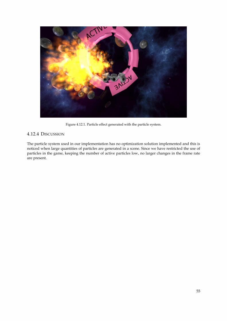
55

Figure 4.12.1. Particle effect generated with the particle system.

4.12.4 DISCUSSION

The particle system used in our implementation has no optimization solution implemented and this is noticed when large quantities of particles are generated in a scene. Since we have restricted the use of particles in the game, keeping the number of active particles low, no larger changes in the frame rate are present.

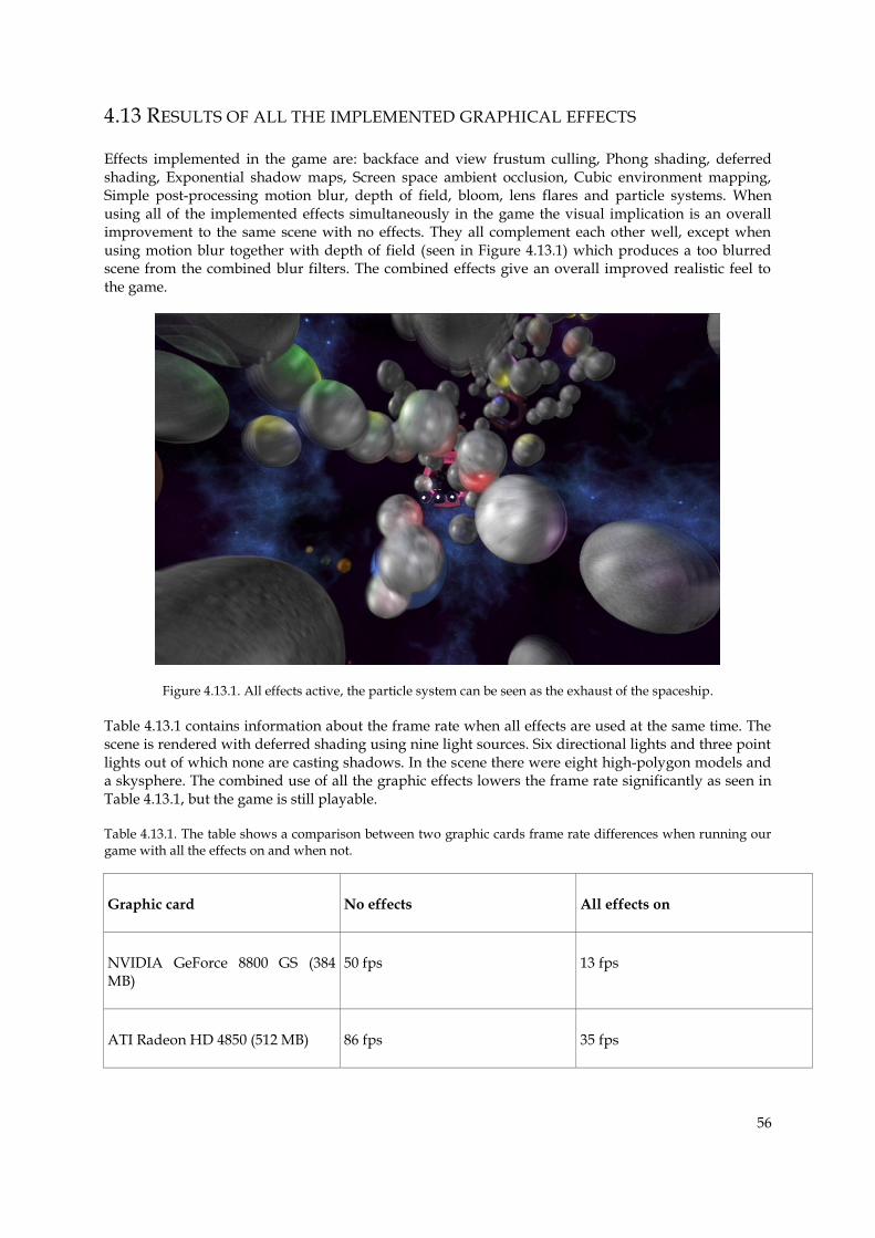
56

4.13 RESULTS OF ALL THE IMPLEMENTED GRAPHICAL EFFECTS

Effects implemented in the game are: backface and view frustum culling, Phong shading, deferred shading, Exponential shadow maps, Screen space ambient occlusion, Cubic environment mapping, Simple post-processing motion blur, depth of field, bloom, lens flares and particle systems. When using all of the implemented effects simultaneously in the game the visual implication is an overall improvement to the same scene with no effects. They all complement each other well, except when using motion blur together with depth of field (seen in Figure 4.13.1) which produces a too blurred scene from the combined blur filters. The combined effects give an overall improved realistic feel to the game.

Figure 4.13.1. All effects active, the particle system can be seen as the exhaust of the spaceship.

Table 4.13.1 contains information about the frame rate when all effects are used at the same time. The scene is rendered with deferred shading using nine light sources. Six directional lights and three point lights out of which none are casting shadows. In the scene there were eight high-polygon models and a skysphere. The combined use of all the graphic effects lowers the frame rate significantly as seen in Table 4.13.1, but the game is still playable.

Table 4.13.1. The table shows a comparison between two graphic cards frame rate differences when running our game with all the effects on and when not.

Graphic card No effects All effects on

NVIDIA GeForce 8800 GS (384 MB)

50 fps 13 fps

ATI Radeon HD 4850 (512 MB) 86 fps 35 fps

57

4.14 DISCUSSION ABOUT ALL THE IMPLEMENTED GRAPHICAL EFFECTS

We are very pleased with how the effects affected the overall visual appearance of the game. They added realism to the game by simulating real-life effects like motion blur and bloom. They all work well together except, as mentioned in the result section, motion blur together with depth of field. We believe that the combined blurring of the scene in the two effects produces the too blurred end result.

We decided to implement our own effects rather than using the effects built into XNA 4.0. One reason was that a large part of the project of creating the game was to implement different effects by ourselves and learn about the techniques available when developing a game. Another reason was that the basic effects provided with XNA 4.0 do not give the option of using more than three directional light sources, and the effects available would not be enough to suite our needs for creating a visually pleasing game.

The base of our rendering pipeline is the deferred shading technique which makes handling of multiple light sources and different materials simpler. To fill our space environment we had to use several lighting effects to create an interesting scene for the player.

When studying Table 4.11.1 it is seen that there is a difference in the frame rate between the graphic cards used for testing. The largest difference between the two GPUs is the bandwidth memory available. Deferred shading uses a large amount of the bandwidth and the different post-process effects add to this strain. This is what causes the frame rate difference and is also the reason the NVIDIA GeForce 8800 GS card has such a low frame rate compared to ATI Radeon HD 4850, with all the effects turned on. With more optimizations of the different techniques, especially the SSAO-effect, the game should be able to render at an acceptable frame rate even on less powerful graphic cards like the NVIDIA GeForce 8800 GS.

When trying to optimize the visual appearance of the effects we encountered a common problem for game developers when the effects looked and performed differently on different GPUs and different screens. The different brands of graphic cards use different standard configurations which gives different visual results. Using different screens proved to be a problem for us as well since the brightness level differed which made the effects look better or worse on the different screens. We resolved this problem by optimizing the effects for one kind of computer for a demo session. An improvement further on would be to make sure that the effects look and perform as similarly as possible on the different screens and GPUs.

All in all we are very pleased with the visual results produced by all of the implemented effects and without them the rendered game would not be as visually pleasing. There are several improvements that could be made to improve both the performance and visual appearance of the effects, the specifics for each effect has been discussed in the discussion sections of the effects. The improvements would take us one step closer to a game that could be marketable.

58

5 MODELING

Modeling is an important part of 3D-game development as it determines the basic shape of an object to be displayed on screen. In this section some software tools for creating models for games and some techniques that can be used when modeling are presented. The chosen software is then presented and discussed.

5.1 INTRODUCTION

The term modeling is used when an artist or engineer utilizes software to create and transform shapes in 3D. Such models can then be implemented in software that uses models in a graphic representation. The following section will introduce software, basic techniques, model types and texturing.

5.2 SOFTWARE

To create models in 3D, a modeling program is used. A modeling program is a tool that utilizes functionalities to make advanced changes on a 3D model. There is a variety of modeling programs with different functionalities and advantages and as such, the following section will introduce the most common programs together with their main advantages.

5.2.1 3DS MAX

3ds max ”provide powerful, integrated 3D modeling, animation, and rendering tools that enable artists and designers to focus more energy on creative, rather than technical challenges.” This program includes extensive polygon and texture mapping toolsets that enable for efficient modeling. (Autodesk, 2012)

5.2.2 MAYA

Maya “animation software delivers a comprehensive creative feature set with tools for animation, modeling, simulation, rendering, matchmoving and compositing on a highly extensible production platform” This program includes an extensive animation User Interface (UI) (Autodesk, 2012).

5.2.3 ZBRUSH

“ZBrush is a digital sculpting and painting program that has revolutionized the 3D industry with its powerful features and intuitive workflows.”. This program has an alternative UI which simulates modeling with clay in a 3D space (Pixologic, 2012).

5.2.4 BLENDER

Blender is a “fully integrated creation suite, offering a broad range of essential tools for the creation of 3D content, including modeling, uv-mapping, texturing, rigging, skinning, animation, particle and other simulation, scripting, rendering, compositing, post-production and game creation”. One of Blender’s advantages is that it is open source and free of charge. Other advantages include that it works cross platform and that its functions enable for efficient modeling (Blender wiki, 2012).

5.2.5 GOOGLE SKETCHUP

”Redecorate your living room. Invent a new piece of furniture. Model your city for Google Earth. There's no limit to what you can create with SketchUp.”. This program utilizes a simplified UI and tools with export functionality specialized for Google Earth (Sketchup Google, 2012).

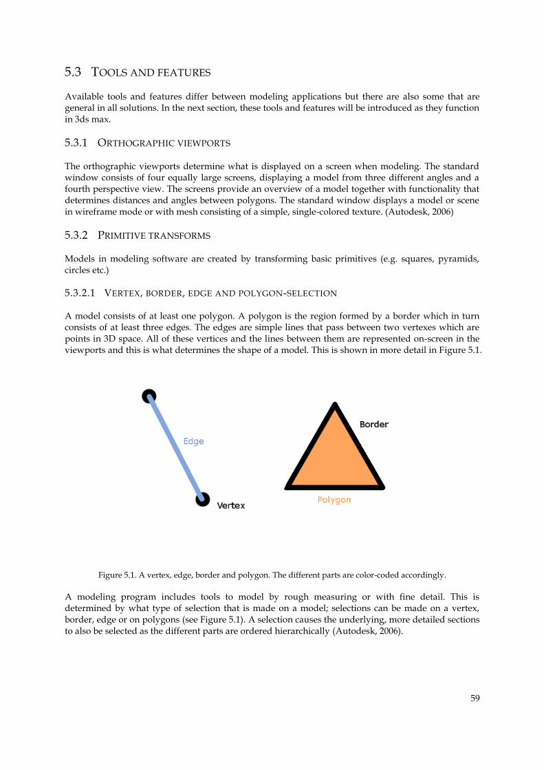
59

5.3 TOOLS AND FEATURES

Available tools and features differ between modeling applications but there are also some that are general in all solutions. In the next section, these tools and features will be introduced as they function in 3ds max.

5.3.1 ORTHOGRAPHIC VIEWPORTS

The orthographic viewports determine what is displayed on a screen when modeling. The standard window consists of four equally large screens, displaying a model from three different angles and a fourth perspective view. The screens provide an overview of a model together with functionality that determines distances and angles between polygons. The standard window displays a model or scene in wireframe mode or with mesh consisting of a simple, single-colored texture. (Autodesk, 2006)

5.3.2 PRIMITIVE TRANSFORMS

Models in modeling software are created by transforming basic primitives (e.g. squares, pyramids, circles etc.)

5.3.2.1 VERTEX, BORDER, EDGE AND POLYGON-SELECTION

A model consists of at least one polygon. A polygon is the region formed by a border which in turn consists of at least three edges. The edges are simple lines that pass between two vertexes which are points in 3D space. All of these vertices and the lines between them are represented on-screen in the viewports and this is what determines the shape of a model. This is shown in more detail in Figure 5.1.

Figure 5.1. A vertex, edge, border and polygon. The different parts are color-coded accordingly.

A modeling program includes tools to model by rough measuring or with fine detail. This is determined by what type of selection that is made on a model; selections can be made on a vertex, border, edge or on polygons (see Figure 5.1). A selection causes the underlying, more detailed sections to also be selected as the different parts are ordered hierarchically (Autodesk, 2006).

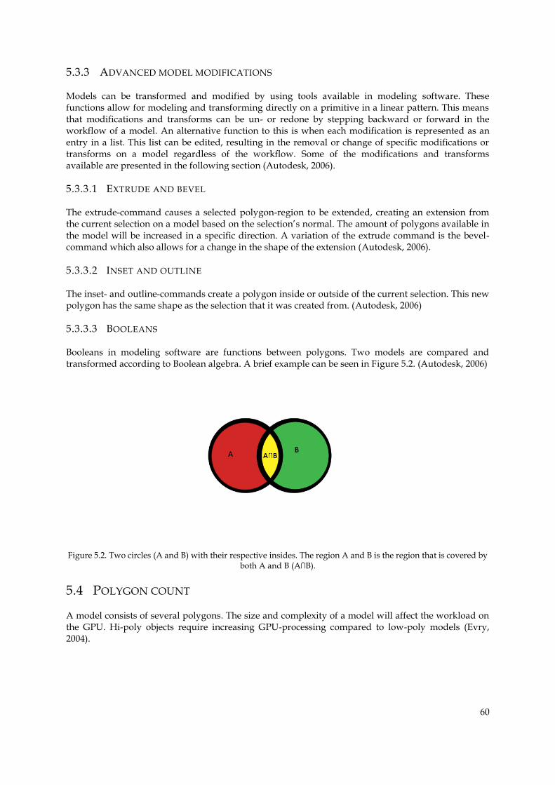
60

5.3.3 ADVANCED MODEL MODIFICATIONS

Models can be transformed and modified by using tools available in modeling software. These functions allow for modeling and transforming directly on a primitive in a linear pattern. This means that modifications and transforms can be un- or redone by stepping backward or forward in the workflow of a model. An alternative function to this is when each modification is represented as an entry in a list. This list can be edited, resulting in the removal or change of specific modifications or transforms on a model regardless of the workflow. Some of the modifications and transforms available are presented in the following section (Autodesk, 2006).

5.3.3.1 EXTRUDE AND BEVEL

The extrude-command causes a selected polygon-region to be extended, creating an extension from the current selection on a model based on the selection’s normal. The amount of polygons available in the model will be increased in a specific direction. A variation of the extrude command is the bevel-command which also allows for a change in the shape of the extension (Autodesk, 2006).

5.3.3.2 INSET AND OUTLINE

The inset- and outline-commands create a polygon inside or outside of the current selection. This new polygon has the same shape as the selection that it was created from. (Autodesk, 2006)

5.3.3.3 BOOLEANS

Booleans in modeling software are functions between polygons. Two models are compared and transformed according to Boolean algebra. A brief example can be seen in Figure 5.2. (Autodesk, 2006)

Figure 5.2. Two circles (A and B) with their respective insides. The region A and B is the region that is covered by both A and B (A∩B).

5.4 POLYGON COUNT

A model consists of several polygons. The size and complexity of a model will affect the workload on the GPU. Hi-poly objects require increasing GPU-processing compared to low-poly models (Evry, 2004).

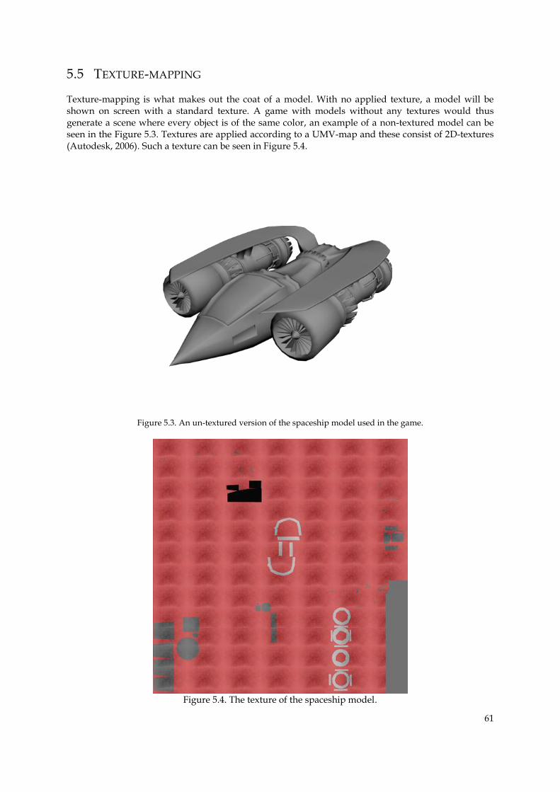
61

5.5 TEXTURE-MAPPING

Texture-mapping is what makes out the coat of a model. With no applied texture, a model will be shown on screen with a standard texture. A game with models without any textures would thus generate a scene where every object is of the same color, an example of a non-textured model can be seen in the Figure 5.3. Textures are applied according to a UMV-map and these consist of 2D-textures (Autodesk, 2006). Such a texture can be seen in Figure 5.4.

Figure 5.3. An un-textured version of the spaceship model used in the game.

Figure 5.4. The texture of the spaceship model.

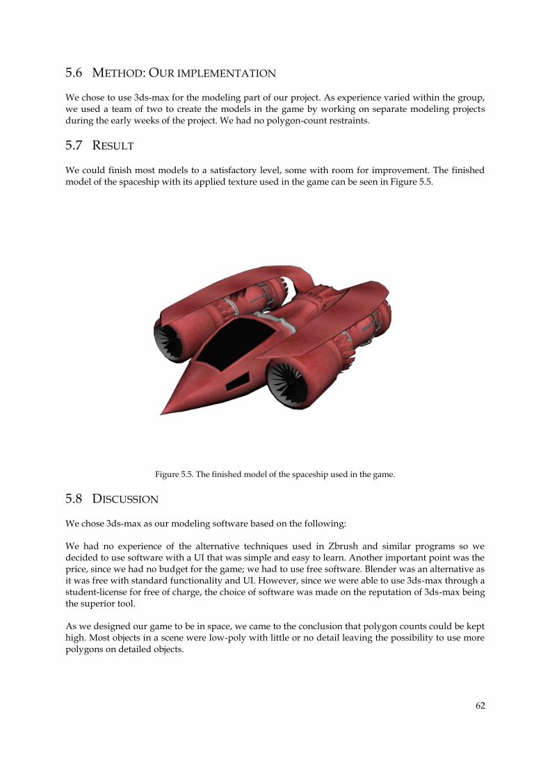
62

5.6 METHOD: OUR IMPLEMENTATION

We chose to use 3ds-max for the modeling part of our project. As experience varied within the group, we used a team of two to create the models in the game by working on separate modeling projects during the early weeks of the project. We had no polygon-count restraints.

5.7 RESULT

We could finish most models to a satisfactory level, some with room for improvement. The finished model of the spaceship with its applied texture used in the game can be seen in Figure 5.5.

Figure 5.5. The finished model of the spaceship used in the game.

5.8 DISCUSSION

We chose 3ds-max as our modeling software based on the following:

We had no experience of the alternative techniques used in Zbrush and similar programs so we decided to use software with a UI that was simple and easy to learn. Another important point was the price, since we had no budget for the game; we had to use free software. Blender was an alternative as it was free with standard functionality and UI. However, since we were able to use 3ds-max through a student-license for free of charge, the choice of software was made on the reputation of 3ds-max being the superior tool.

As we designed our game to be in space, we came to the conclusion that polygon counts could be kept high. Most objects in a scene were low-poly with little or no detail leaving the possibility to use more polygons on detailed objects.

63

6 PHYSICS

Physics in games refers to the set of rules and principles that determine how material objects in the game world react to collisions with other players and objects, gravity and other sources of influence. In this section, some relevant theory behind game physics, mechanics, collision detection and collision response will be presented. Then, a description of the algorithms implemented in our game will follow. Finally, the actual results of the implementation will be presented and discussed.

6.1 INTRODUCTION

Within the game field, the terms physics or game physics typically refer to some form of numerical implementation of classical mechanics (games that involve magnetic forces of some sort use principles from electromagnetism, a different subfield of physics, for that element). Classical mechanics is the science that describes how macroscopic material objects move and interact with speeds, forces, acceleration, translations, rotations, collisions and so on.

In this section two topics will be covered; motion and collision. Motion is the time-dependent path of some material object resulting from forces and torques. Examples include the movement of a rally car driving on a road, a character running on a floor, or a stone thrown in the air. A collision occurs when two objects have been approaching one another and are very close. The field of collisions covers different interactions of simulated material entities. The field of collisions can be divided into two main subfields; collision detection and collision response. Collision detection typically deals with detecting intersections between geometrical entities which are then spatially separated from one another. Collision response is what determines what will happen as a result of a collision, e.g. bounces, explosions, resting contact etc.

6.2 ORDINARY DIFFERENTIAL EQUATIONS

A large amount of physics problems, such as determining the motion of projectiles or bodies moving in free space, deal with ordinary differential equations or ODEs (Giordano, 2006). ODEs and their solutions are central in simulating the movements of objects in a game. Specifically, the simulation relies heavily on an ODE called Newton’s second law (Newton II). When implemented in a game, Newton II can give the center of mass acceleration for each moving object for a specific time in the game. Using numerical ODE solution methods, the corresponding velocity and position can then be obtained.

An ODE is an equation describing the relationship between some function and a number of its derivatives. An ODE problem is some specific ODE together with one or several boundary conditions. One special case of ODE problems is the boundary value problem for a first order ODE, which can be expressed mathematically as in equation 6.1.

𝑦′ ( 𝑦 ) ≤ ≤ 𝑏

𝑦 (6.1)

Here, t is some parameter such as time, 𝑦 is the function, 𝑦′ its derivative with respect to and is some function.

There are a number of methods for solving the differential equations numerically. Those methods vary in a number of aspects such as accuracy and stability. The lower demands on accuracy in games (compared to applications in science or engineering), as well as ease of implementation are two major factors in the choice of an integration algorithm for a specific game or game engine.

64

Numerical ODE solution methods can be divided into two major categories: implicit methods and explicit methods. Explicit methods yield the value for the next time step directly from a formula, whereas implicit methods in addition require the solution of a non-linear equation for every time step, which adds to the computational cost (Gustafsson, 2010). Implicit methods can be useful for stiff problems, i.e. problems that are susceptible to numerical instability issues unless a very small time step is used.

A common algorithm for games is the Euler forward method. The scheme for this method is shown in equation 6.2.

𝑦 𝑦 ∆ 𝑦 ′

𝑦 (6.2)

Given a previous value 𝑦 of the function 𝑦 at time and some time step ∆ , this scheme gives the

value 𝑦 for time . is some constant. 𝑦 is the value at the start of the interval for , i.e. 𝑦 . 𝑦

is the derivative at time .

The main reason for using this method is its simplicity (so the time the game programmer needs to spend learning the method is reasonably short). Unfortunately, the method is relatively unstable and inaccurate (Eberly, 2004). In a game, these shortcomings can cause two types of problems. The instability can cause the movements of in-game objects to react unpredictably such as growing to excessive values. The inaccuracy means that movements will deviate from movements generated by a theoretical exact solution of the ODE.

Another method which is popular in some game engines is the explicit Runge-Kutta 4 method (RK4). RK4 is considerably more stable and accurate than Euler forward, while still being relatively computationally cheap.

6.3 NEWTONIAN MECHANICS

This section will present the basic theory of Newtonian mechanics, which is the theory that game physics is based on.

6.3.1 POSITION, VELOCITY AND ACCELERATION

In Newtonian mechanics, the position and movement of a point in space can be described by three three-dimensional vector quantities: position, velocity and acceleration. The position vector is a set of three real-valued numbers, which give the coordinates of the point in space. The velocity vector describes how the position vector changes with time and, equivalently, the acceleration vector tells us how the velocity vector changes as time passes. Formally velocity is the time derivative of position and acceleration is the time derivative of velocity. This can be described mathematically as in equation 6.3.

𝒗 �̇�

𝒂 �̇� (6.3)

Here, p is the position, v is the velocity and a is the acceleration. A vector with a dot notation on top means the time-derivative of the vector below the dot and is standard in the field of mechanics. An alternative way of describing a time derivative is with Leibniz’s notation, which is used extensively in various mathematical fields, such as calculus. With this notation, the first equation would be written as equation 6.4.

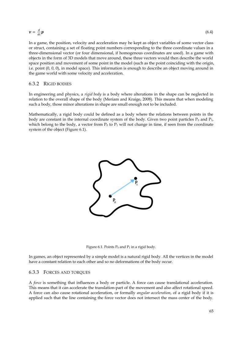
65

𝒗

𝒑 (6.4)

In a game, the position, velocity and acceleration may be kept as object variables of some vector class or struct, containing a set of floating point numbers corresponding to the three coordinate values in a three-dimensional vector (or four dimensional, if homogenous coordinates are used). In a game with objects in the form of 3D models that move around, these three vectors would then describe the world space position and movement of some point in the model (such as the point coinciding with the origin, i.e. point (0, 0, 0), in model space). This information is enough to describe an object moving around in the game world with some velocity and acceleration.

6.3.2 RIGID BODIES

In engineering and physics, a rigid body is a body where alterations in the shape can be neglected in relation to the overall shape of the body (Meriam and Kraige, 2008). This means that when modeling such a body, those minor alterations in shape are small enough not to be included.

Mathematically, a rigid body could be defined as a body where the relations between points in the body are constant in the internal coordinate system of the body. Given two point particles P0 and P1, which belong to the body, a vector from P0 to P1 will not change in time, if seen from the coordinate system of the object (Figure 6.1).

Figure 6.1. Points P0 and P1 in a rigid body.

In games, an object represented by a simple model is a natural rigid body. All the vertices in the model have a constant relation to each other and so no deformations of the body occur.

6.3.3 FORCES AND TORQUES

A force is something that influences a body or particle. A force can cause translational acceleration. This means that it can accelerate the translation-part of the movement and also affect rotational speed. A force can also cause rotational acceleration, or formally angular acceleration, of a rigid body if it is applied such that the line containing the force vector does not intersect the mass center of the body.

66

The cross product of such a force and a vector from the mass center of the body to the point of application is known as a torque:

(6.5)

In equation 6.5, is the torque applied at a point with vector and F is the force.

6.3.4 NEWTON’S LAWS OF MOTION

Isaac Newton came up with three laws of the motion of material objects, which are still being used widely today. The first law says that an object will remain still or continue with constant velocity unless a force is applied. The second law, also known as Newton II, states that the sum of all forces acting on an object is equal to the mass of the object multiplied by its acceleration. The second law gives an exact mathematical description of the way forces cause acceleration. Mathematically, the law can be expressed as seen in equation 6.6.

𝐚 (6.6)

In equation 6.6, F denotes the total force acting on some object. That means that it is really a sum of possibly a large number of different forces such as engine thrust, gravity, friction, wind, magnetic forces and so on. The symbol m means the total mass of the object. a is the acceleration, as before. According to Newton’s third law, for every force there is an opposite force with equal magnitude. “Opposite” here means that the force vector is in a direction opposite to the other force vector.

Of these three laws, the second and third are highly relevant and highly applicable to game physics. With the second law, we can get a new acceleration for every iteration and for every moving object in the game by first collecting all the different forces currently acting on the object into some vector variable, and then simply solving for the acceleration vector equation 6.6 to get the updated acceleration of the object.

6.3.5 MOMENTUM

Momentum is the product of mass and velocity as seen in equation 6.7.

𝐩 𝐯 (6.7)

In equation 6.7, p is the momentum, m is the mass and v is the velocity. Momentum is sometimes used to describe the motion of some object rather than the velocity, if it is useful to consider the velocity and mass together. An important example is Newton II, which can be expressed alternatively with momentum as F=ṗ, i.e. the (total) force equals the time derivative of the momentum.

6.3.6 IMPULSES

An impulse is a vector that changes the momentum of some object by addition; an impulse can be seen as simply an “addition of momentum”. Specifically, impulse is an integral sum of force varying over time (equation 6.8).

𝐉 ∫

(6.8)

In equation 6.8, J is the impulse, F is the force, t1 is the time at the start of the application of the force, and t2 is the time when the application ends.

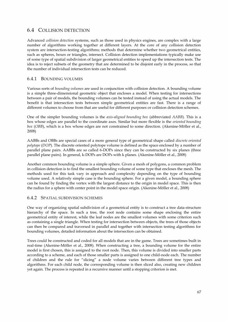
67

6.4 COLLISION DETECTION

Advanced collision detection systems, such as those used in physics engines, are complex with a large number of algorithms working together at different layers. At the core of any collision detection system are intersection-testing algorithms; methods that determine whether two geometrical entities, such as spheres, boxes or triangles, intersect. Collision detection implementations typically make use of some type of spatial subdivision of larger geometrical entities to speed up the intersection tests. The idea is to reject subsets of the geometry that are determined to be disjoint early in the process, so that the number of individual intersection tests can be reduced.

6.4.1 BOUNDING VOLUMES

Various sorts of bounding volumes are used in conjunction with collision detection. A bounding volume is a simple three-dimensional geometric object that encloses a model. When testing for intersections between a pair of models, the bounding volumes can be tested instead of using the actual models. The benefit is that intersection tests between simple geometrical entities are fast. There is a range of different volumes to choose from that are useful for different purposes or collision detection schemes.

One of the simpler bounding volumes is the axis-aligned bounding box (abbreviated AABB). This is a box whose edges are parallel to the coordinate axes. Similar but more flexible is the oriented bounding box (OBB), which is a box whose edges are not constrained to some direction. (Akenine-Möller et al., 2008)

AABBs and OBBs are special cases of a more general type of geometrical shape called discrete oriented polytope (DOP). The discrete oriented polytope volume is defined as the space enclosed by a number of parallel plane pairs. AABBs are so called 6-DOPs since they can be constructed by six planes (three parallel plane pairs). In general, k-DOPs are DOPs with k planes. (Akenine-Möller et al., 2008)

Another common bounding volume is a simple sphere. Given a mesh of polygons, a common problem in collision detection is to find the smallest bounding volume of some type that encloses the mesh. The methods used for this task vary in approach and complexity depending on the type of bounding volume used. A relatively simple case is the bounding sphere. For a given model, a bounding sphere can be found by finding the vertex with the largest distance to the origin in model space. This is then the radius for a sphere with center point in the model space origin. (Akenine-Möller et al., 2008)

6.4.2 SPATIAL SUBDIVISION SCHEMES

One way of organizing spatial subdivision of a geometrical entity is to construct a tree data-structure hierarchy of the space. In such a tree, the root node contains some shape enclosing the entire geometrical entity of interest, while the leaf nodes are the smallest volumes with some criterion such as containing a single triangle. When testing for intersection between objects, the trees of those objects can then be compared and traversed in parallel and together with intersection testing algorithms for bounding volumes, detailed information about the intersection can be obtained.

Trees could be constructed and coded for all models that are in the game. Trees are sometimes built in real-time (Akenine-Möller et al., 2008). When constructing a tree, a bounding volume for the entire model is first chosen, this is assigned to the root node. Then, this volume is divided into smaller parts according to a scheme, and each of those smaller parts is assigned to one child-node each. The number of children and the rule for “slicing” a node volume varies between different tree types and algorithms. For each child node, the corresponding volume is then sliced also, creating new children yet again. The process is repeated in a recursive manner until a stopping criterion is met.

68

A simpler tree presented in Akenine-Möller et al. (2008) is the quad-tree. Here, each node is split in eight children, whose volumes are equally large. Similar to this is the octree, a tree type used mostly for two-dimensional entities, where there are four equally large children.

Gottschalk (1996) presents his OBB-tree, also mentioned in Akenine-Möller et al. (2008). The OBB-tree is a binary tree (which means that each non-leaf node has two children), where node volumes are OBBs. When splitting a node, the longest axis of the box is first determined. A splitting plane with the normal parallel with this axis is then chosen. The location of the plane along the axis is found by taking the mean of the centroids (mean of vertices) of the triangles contained in the box.

6.4.3 INTERSECTIONS TESTS

Intersection testing algorithms are usually present at the lower levels of a collision detection system. For example, they can be used in tree hierarchy intersection checks to find intersecting leaf nodes, as described above. If it is know that the leaf nodes each contain a single triangle, triangle-triangle intersection can then be used to see if the triangles intersect.

For intersection testing between various bounding volumes, triangles and line segments, there is a useful theorem called the separating axis theorem (SAT) which is the basis for several popular intersection testing algorithms for these shapes. SAT says that two objects are disjoint if and only if there exists an axis on which the objects do not intersect. Akenine-Möller et al. (2008) presents an algorithm based on the SAT to check for intersection between triangles.

For triangle/OBB or triangle/AABB tests, Gottschalk (1996) presents an algorithm using SAT that has been proved to be significantly faster than previously suggested methods which used closest features and linear programming.

6.4.4 COLLISION DETECTION SYSTEMS

In a world with many simultaneously moving objects, so called multiphase collision detection systems can be useful. The idea is to have an initial rough phase of collision detection which only potentially colliding objects pass. Those potentially colliding objects then go on the next phases, each more precise than the previous one. One algorithm for providing the rough initial phase is the Sweep-And-Prune algorithm.

6.5 COLLISION RESPONSE

Given a set of objects that have been detected to collide, collision response determines what is going to happen as a consequence of the collision. For example, the objects could simply bounce off each other. They might also undergo some form of destruction, in case they are destructible objects. Another alternative is that parts from both objects will be still relative to each other after the collision, a concept known as resting contact.

A simple collision response (Akenine-Möller et al., 2008) is to treat two colliding objects as frictionless, non-deformable spheres at the instant of collision, calculate new velocities with mechanics formulas for particle collisions, and set those new velocities to the objects instantly. Depending on the specific collision formula used, the resulting collision may be elastic, that is when all kinetic energy is conserved, or inelastic meaning some kinetic energy has been lost as a result of the collision.

Assume that two objects have been detected to collide, and have been spatially separated (so that they are close but do not intersect). A rotation of the coordinate axes is then performed so that each velocity vector has one component parallel with the line of collision. Now the situation can be treated as a one dimensional collision with those velocities. The other velocity component is perpendicular to the line of collision and therefore does not contribute to the collision. This means that a formula for a one-

69

dimensional collision can be used to get new collision line velocities, while the perpendicular components are left unchanged.

A formula for a one-dimensional collision between two spherical objects can be derived by setting up and solving set of equations. For an elastic collision, this corresponds to the conditions that both momentum and kinetic energy are conserved after the collision.

′

′

′

′ (6.9)

Here in equation 6.9, and are the masses of the two objects, and the initial velocities, and

′ and ′ the post-collision velocities. Solving this set of equations yields a formula that gives

′ and

′ directly. In the code, this gives the post-collision velocities in the rotated system and after a rotation back to the original system, the task is completed.

Baraff (1997) presents a more sophisticated collision response approach that allows for realistic rotations and resting contact. Baraff treats the colliding objects as rigid bodies with some shape (which could coincide with the hull of the model). At collisions, objects then affect each other by force or impulse vectors applied at the collision points. For impulse collisions, that is collisions after which resting contact is not achieved, impulse vectors are used. To derive expressions for the impulses, the author sets up a system of equations which he solves analytically, yielding an expression for an impulse vector which depends on pre-collision velocities and moment of inertia. For resting contact, a number of constraints are set up in the form of equations of which the resulting system is then solved numerically in the code.

6.6 METHOD: OUR IMPLEMENTATION

Rather than using an available physics engine, we decided on creating our own solution from scratch. We implemented a simple physics engine with support for forces, collision detection, and collision response.

For the collision detection, we implemented a two-phase system. At the broad-phase stage, we use our own implementation of the Sweep-And-Prune algorithm as presented in Akenine-Möller et al. (2008). For every object in its internal list, the SAP code uses AABBs whose sides are equal to the bounding sphere radius. The second phase of the collision detection system then tests for intersection between OBBs for the models of the objects involved. A combined collision resolution and collision point determination is then performed. Where the bounding spheres of the colliding objects are considered, which are separated along with their objects along the axis that contains the vector from the center point of one sphere to the center point of the other sphere see Figure 6.2.

70

Figure 6.2. Collision between bounding spheres.

For collision response we implemented the simple collision response variant mentioned in Akenine-Möller et al. (2008).

For the force system, we used a scheme where all the different forces that can affect an object are collected into a force vector which is a class member variable. A force, such as engine thrust or gravity (although we have not implemented this) is collected into the force vector by adding itself to it. For a given iteration, the objects force vector is zero from the start. All the different forces that are going to affect the object are then added in the manner described above. In this way, a resultant force vector is finally obtained. Then, an update-method in the object is called, where the acceleration corresponding to the resultant force is determined using Newton II. Numerical integration code thereafter follows to determine the new velocity and position.

6.6.1 SPACESHIP MOVEMENT

The movement of the spaceship in the game is governed by a control system that uses principles from the field of control theory. The overall aim of the system was to make a flexible solution where both realism and user friendliness could be varied relatively easily in the code. Thus, with our solution, a new control system can be created relatively quickly by minor changes in the code.

6.7 RESULT

The force system works as it should. Forces are added to each object’s internal force vector, and acceleration, velocity and position values are updated in a correct manner.

The collision system also works as expected. Thanks to the ability of the multi-phase system to handle many simultaneously moving objects, we can have a large number of colliding entities at the same time without putting a considerable strain on overall performance in the game.

6.8 DISCUSSION

We decided to make our own physics implementation rather than using an existing engine. The idea was that making our own engine would require learning all the different algorithms more in-depth and therefore gain a more comprehensive and detailed understanding of them. It also seemed

71

appealing to be able to have full control over every detail in the physics system, increasing our ability to make our own customizations. In the end, all of those positive aspects have turned out to be true. Articles about algorithms, such as the SAT system and OBB-intersection, have been read thoroughly after which an implementation in code has been written.

On the other hand, choosing an existing physics engine would require learning all the specifics about structure, function and implementation. The focus would likely be on engine-specific technical details rather than on algorithms.

An advantage of using an existing engine, however, is that we would have a highly advanced engine ready from the start, including some features that we did not have time to implement in our own engine. For example, physics engines typically have robust implementations of triangle-level collisions detection, impulse reactions and resting contact. Our original plan was to implement these features in our own engine. However, doing this turned out to be more difficult than expected.

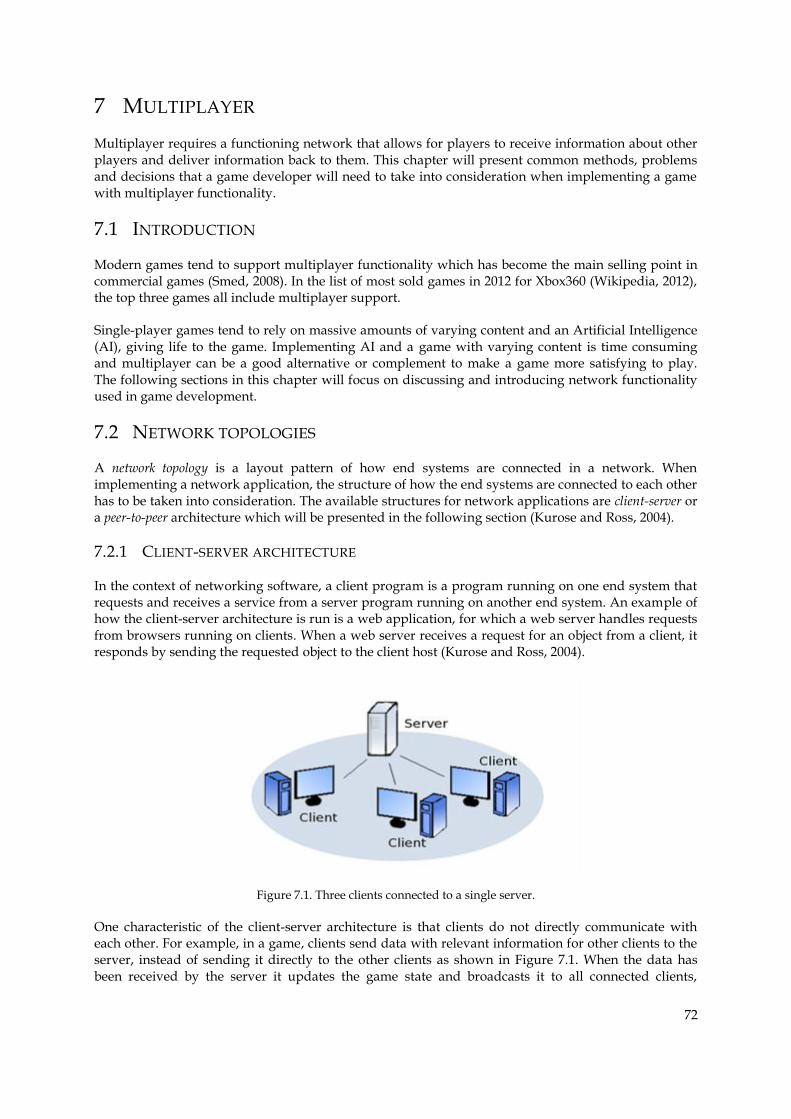
72

7 MULTIPLAYER

Multiplayer requires a functioning network that allows for players to receive information about other players and deliver information back to them. This chapter will present common methods, problems and decisions that a game developer will need to take into consideration when implementing a game with multiplayer functionality.

7.1 INTRODUCTION

Modern games tend to support multiplayer functionality which has become the main selling point in commercial games (Smed, 2008). In the list of most sold games in 2012 for Xbox360 (Wikipedia, 2012), the top three games all include multiplayer support.

Single-player games tend to rely on massive amounts of varying content and an Artificial Intelligence (AI), giving life to the game. Implementing AI and a game with varying content is time consuming and multiplayer can be a good alternative or complement to make a game more satisfying to play. The following sections in this chapter will focus on discussing and introducing network functionality used in game development.

7.2 NETWORK TOPOLOGIES

A network topology is a layout pattern of how end systems are connected in a network. When implementing a network application, the structure of how the end systems are connected to each other has to be taken into consideration. The available structures for network applications are client-server or a peer-to-peer architecture which will be presented in the following section (Kurose and Ross, 2004).

7.2.1 CLIENT-SERVER ARCHITECTURE

In the context of networking software, a client program is a program running on one end system that requests and receives a service from a server program running on another end system. An example of how the client-server architecture is run is a web application, for which a web server handles requests from browsers running on clients. When a web server receives a request for an object from a client, it responds by sending the requested object to the client host (Kurose and Ross, 2004).

Figure 7.1. Three clients connected to a single server.

One characteristic of the client-server architecture is that clients do not directly communicate with each other. For example, in a game, clients send data with relevant information for other clients to the server, instead of sending it directly to the other clients as shown in Figure 7.1. When the data has been received by the server it updates the game state and broadcasts it to all connected clients,

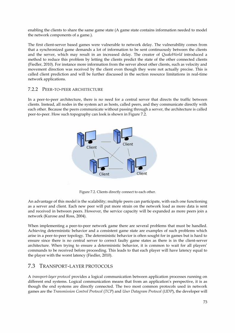
73

enabling the clients to share the same game state (A game state contains information needed to model the network components of a game.).

The first client-server based games were vulnerable to network delay. The vulnerability comes from that a synchronized game demands a lot of information to be sent continuously between the clients and the server, which may result in an increased delay. The creator of QuakeWorld introduced a method to reduce this problem by letting the clients predict the state of the other connected clients (Fiedler, 2010). For instance more information from the server about other clients, such as velocity and movement direction was received by the client even though they were not actually precise. This is called client prediction and will be further discussed in the section resource limitations in real-time network applications.

7.2.2 PEER-TO-PEER ARCHITECTURE

In a peer-to-peer architecture, there is no need for a central server that directs the traffic between clients. Instead, all nodes in the system act as hosts, called peers, and they communicate directly with each other. Because the peers communicate without passing through a server, the architecture is called peer-to-peer. How such topography can look is shown in Figure 7.2.

Figure 7.2. Clients directly connect to each other.

An advantage of this model is the scalability; multiple peers can participate, with each one functioning as a server and client. Each new peer will put more strain on the network load as more data is sent and received in between peers. However, the service capacity will be expanded as more peers join a network (Kurose and Ross, 2004).

When implementing a peer-to-peer network game there are several problems that must be handled. Achieving deterministic behavior and a consistent game state are examples of such problems which arise in a peer-to-peer topology. The deterministic behavior is often sought for in games but is hard to ensure since there is no central server to correct faulty game states as there is in the client-server architecture. When trying to ensure a deterministic behavior, it is common to wait for all players’ commands to be received before proceeding. This leads to that each player will have latency equal to the player with the worst latency (Fiedler, 2010).

7.3 TRANSPORT-LAYER PROTOCOLS

A transport-layer protocol provides a logical communication between application processes running on different end systems. Logical communication means that from an application’s perspective, it is as though the end systems are directly connected. The two most common protocols used in network games are the Transmission Control Protocol (TCP) and User Datagram Protocol (UDP), the developer will

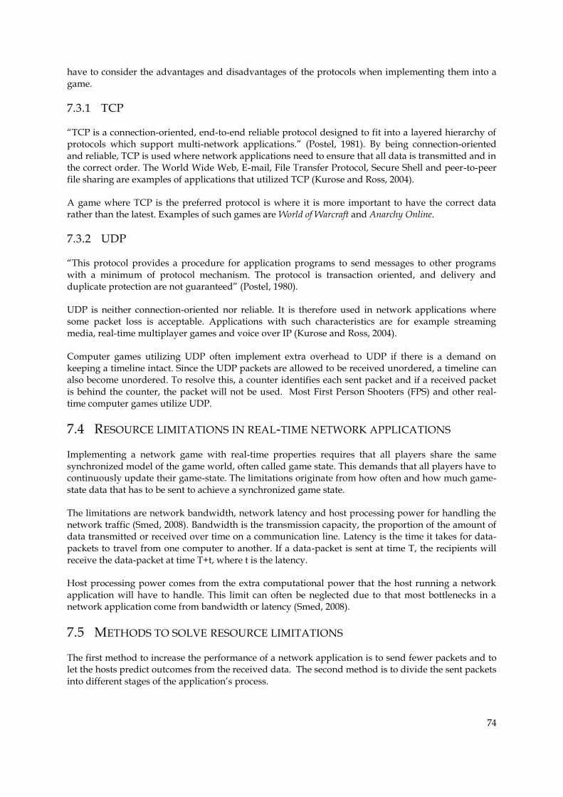
74

have to consider the advantages and disadvantages of the protocols when implementing them into a game.

7.3.1 TCP

“TCP is a connection-oriented, end-to-end reliable protocol designed to fit into a layered hierarchy of protocols which support multi-network applications.” (Postel, 1981). By being connection-oriented and reliable, TCP is used where network applications need to ensure that all data is transmitted and in the correct order. The World Wide Web, E-mail, File Transfer Protocol, Secure Shell and peer-to-peer file sharing are examples of applications that utilized TCP (Kurose and Ross, 2004).

A game where TCP is the preferred protocol is where it is more important to have the correct data rather than the latest. Examples of such games are World of Warcraft and Anarchy Online.

7.3.2 UDP

“This protocol provides a procedure for application programs to send messages to other programs with a minimum of protocol mechanism. The protocol is transaction oriented, and delivery and duplicate protection are not guaranteed” (Postel, 1980).

UDP is neither connection-oriented nor reliable. It is therefore used in network applications where some packet loss is acceptable. Applications with such characteristics are for example streaming media, real-time multiplayer games and voice over IP (Kurose and Ross, 2004).

Computer games utilizing UDP often implement extra overhead to UDP if there is a demand on keeping a timeline intact. Since the UDP packets are allowed to be received unordered, a timeline can also become unordered. To resolve this, a counter identifies each sent packet and if a received packet is behind the counter, the packet will not be used. Most First Person Shooters (FPS) and other real-time computer games utilize UDP.

7.4 RESOURCE LIMITATIONS IN REAL-TIME NETWORK APPLICATIONS

Implementing a network game with real-time properties requires that all players share the same synchronized model of the game world, often called game state. This demands that all players have to continuously update their game-state. The limitations originate from how often and how much game-state data that has to be sent to achieve a synchronized game state.

The limitations are network bandwidth, network latency and host processing power for handling the network traffic (Smed, 2008). Bandwidth is the transmission capacity, the proportion of the amount of data transmitted or received over time on a communication line. Latency is the time it takes for data-packets to travel from one computer to another. If a data-packet is sent at time T, the recipients will receive the data-packet at time T+t, where t is the latency.

Host processing power comes from the extra computational power that the host running a network application will have to handle. This limit can often be neglected due to that most bottlenecks in a network application come from bandwidth or latency (Smed, 2008).

7.5 METHODS TO SOLVE RESOURCE LIMITATIONS

The first method to increase the performance of a network application is to send fewer packets and to let the hosts predict outcomes from the received data. The second method is to divide the sent packets into different stages of the application’s process.

75

Combinations where both methods are used are common in games, for instance many real-time games utilize prediction by sending fewer packets and this is called client-predication or dead-reckoning (Aronson, 1997).

7.5.1 CLIENT PREDICTION

With client prediction, every client is simulating all or some entities in a game, though with a coarse level of fidelity. The predication is done by algorithms that extrapolate behavior of entities at a set level of how far reality should be allowed to get from the extrapolating before a correction is issued (Aronson, 1997). The correction is the real state of the entity we did a prediction of.

In a game with moving entities, client predication (as seen in Figure 7.3) often utilizes velocity and direction data to predict the path of a moving entity. For example at time t0 on position x, the entity has a velocity of v. The client calculates the position at time t1 as x+v*t1 and simulate the movement from x to y*t1 in time t1 – t0. When a correction is issued the simulated value will be compared to the correct one and with a set threshold, the algorithm decides if a correction shall override the simulated value or not. By using this method a game will abolish latency issues at the cost of data consistency (Smed et al., 2002).

Figure 7.3. Here is an example of three predictions, occurring at different times. The client uses these predictions to render the object until a correction occurs where it will do a new prediction. At 0 seconds the object is moving

forward, at 0.3 seconds the ship has started to turn clockwise, and at 0.5 seconds it is going straight forward again.

7.6 DIVIDING GAME-STATE UPDATES INTO DIFFERENT FRAMES

Sending all state updates at the same time or in every update is often unnecessary. A lot of data is independent of each other and sending all the data at the same time can lead to a bottleneck in the application causing temporary freezes which occur when a client receives (and has to process) a lot of data. Consider an example with ten clients where a client has to perform a 5ms computation per client (for example rendering a player entity). Then there will be a 50ms break in the game and at this stage the user experience may not have been reduced. But with a linear scaling of longer brakes per connected user, the game may turn unplayable. If updates are sent only once in ten frames, the amount of data sent and processed would be reduced to 90%. Client-prediction could be used to compensate the smaller amount of data sent, to retain an illusion of real-time gameplay.

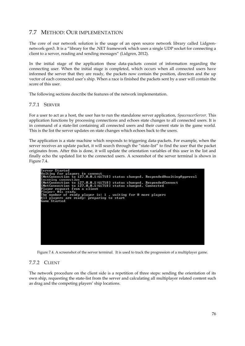
76

7.7 METHOD: OUR IMPLEMENTATION

The core of our network solution is the usage of an open source network library called Lidgren-network-gen3. It is a “library for the .NET framework which uses a single UDP socket for connecting a client to a server, reading and sending messages“ (Lidgren, 2012).

In the initial stage of the application these data-packets consist of information regarding the connecting user. When the initial stage is completed, which occurs when all connected users have informed the server that they are ready, the packets now contain the position, direction and the up vector of each connected user’s ship. When a race is finished the packets sent by a user will contain the score of this user.

The following sections describe the features of the network implementation.

7.7.1 SERVER

For a user to act as a host, the user has to run the standalone server application, SpaceracerServer. This application functions by processing connections and echoes state changes to all connected users. It is in command of a state-list containing all connected users and their current state in the game world. This is the list the server updates on state changes which echoes back to the users.

The application is a state machine which responds to triggering data-packets. For example, when the server receives an update packet, it will search through the “state-list” to find the user that the packet originates from. After this is done, it will update the orientation variables of this user in the list and finally echo the updated list to the connected users. A screenshot of the server terminal is shown in Figure 7.4.

Figure 7.4. A screenshot of the server terminal. It is used to track the progression of a multiplayer game.

7.7.2 CLIENT

The network procedure on the client side is a repetition of three steps: sending the orientation of its own ship, requesting the state-list from the server and calculating all multiplayer related content such as drag and the competing players’ ship locations.

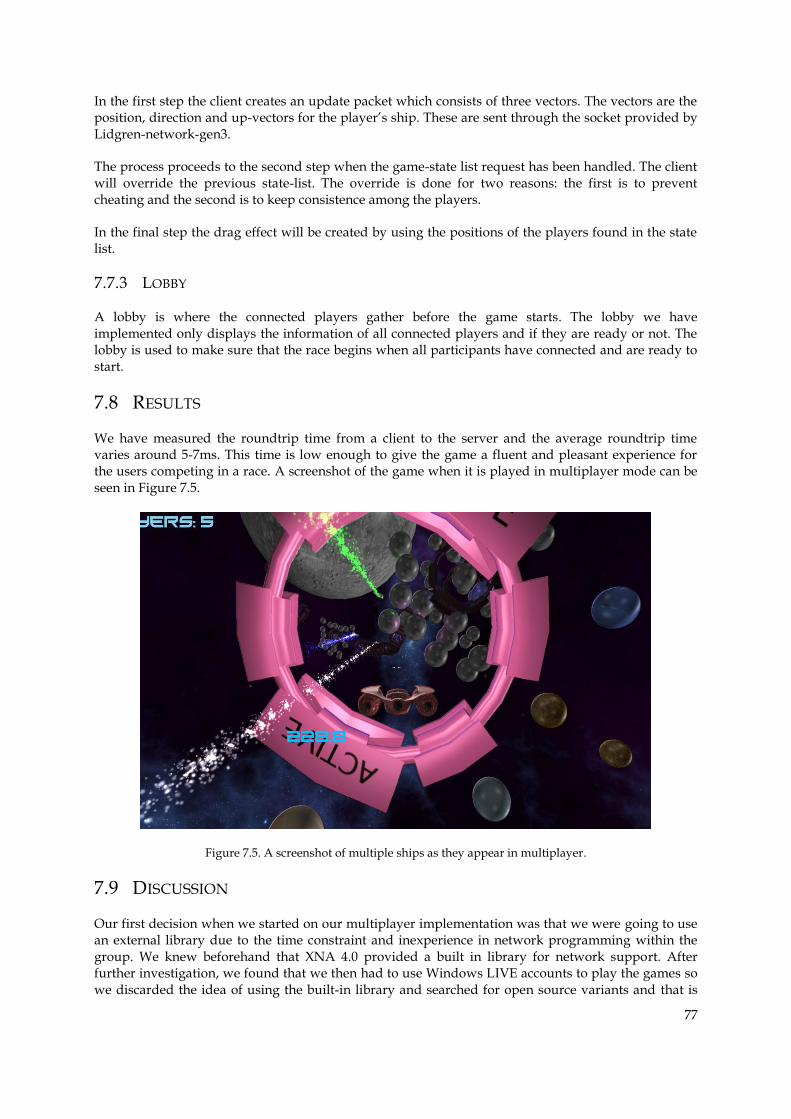
77

In the first step the client creates an update packet which consists of three vectors. The vectors are the position, direction and up-vectors for the player’s ship. These are sent through the socket provided by Lidgren-network-gen3.

The process proceeds to the second step when the game-state list request has been handled. The client will override the previous state-list. The override is done for two reasons: the first is to prevent cheating and the second is to keep consistence among the players.

In the final step the drag effect will be created by using the positions of the players found in the state list.

7.7.3 LOBBY

A lobby is where the connected players gather before the game starts. The lobby we have implemented only displays the information of all connected players and if they are ready or not. The lobby is used to make sure that the race begins when all participants have connected and are ready to start.

7.8 RESULTS

We have measured the roundtrip time from a client to the server and the average roundtrip time varies around 5-7ms. This time is low enough to give the game a fluent and pleasant experience for the users competing in a race. A screenshot of the game when it is played in multiplayer mode can be seen in Figure 7.5.

Figure 7.5. A screenshot of multiple ships as they appear in multiplayer.

7.9 DISCUSSION

Our first decision when we started on our multiplayer implementation was that we were going to use an external library due to the time constraint and inexperience in network programming within the group. We knew beforehand that XNA 4.0 provided a built in library for network support. After further investigation, we found that we then had to use Windows LIVE accounts to play the games so we discarded the idea of using the built-in library and searched for open source variants and that is

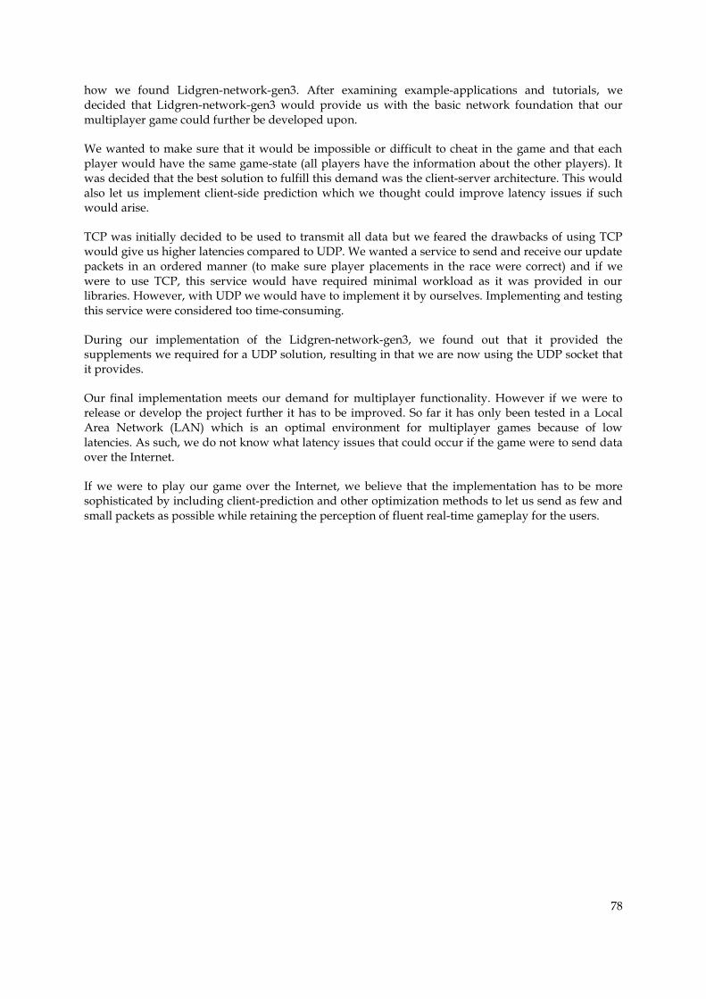
78

how we found Lidgren-network-gen3. After examining example-applications and tutorials, we decided that Lidgren-network-gen3 would provide us with the basic network foundation that our multiplayer game could further be developed upon.

We wanted to make sure that it would be impossible or difficult to cheat in the game and that each player would have the same game-state (all players have the information about the other players). It was decided that the best solution to fulfill this demand was the client-server architecture. This would also let us implement client-side prediction which we thought could improve latency issues if such would arise.

TCP was initially decided to be used to transmit all data but we feared the drawbacks of using TCP would give us higher latencies compared to UDP. We wanted a service to send and receive our update packets in an ordered manner (to make sure player placements in the race were correct) and if we were to use TCP, this service would have required minimal workload as it was provided in our libraries. However, with UDP we would have to implement it by ourselves. Implementing and testing this service were considered too time-consuming.

During our implementation of the Lidgren-network-gen3, we found out that it provided the supplements we required for a UDP solution, resulting in that we are now using the UDP socket that it provides.

Our final implementation meets our demand for multiplayer functionality. However if we were to release or develop the project further it has to be improved. So far it has only been tested in a Local Area Network (LAN) which is an optimal environment for multiplayer games because of low latencies. As such, we do not know what latency issues that could occur if the game were to send data over the Internet.

If we were to play our game over the Internet, we believe that the implementation has to be more sophisticated by including client-prediction and other optimization methods to let us send as few and small packets as possible while retaining the perception of fluent real-time gameplay for the users.

79

8 RESULTS FOR ALL THE TECHNIQUES IMPLEMENTED

A fully playable game with functionality in the areas of graphical effects, physics and network has been completed. After research in the different fields covered in this report, the algorithms and methods best suited for our game have been selected and implemented.

The final version of our software implementation is a racing game in an open space environment where players can race alone or with human opponents to fly from start to finish along a track as fast as possible. The track is defined by waypoints, which the players must follow in the correct order from start to finish. Throughout the track are obstacles in the form is spherical-shaped asteroids, which cause a player to loose speed and bounce away at a collision. Speed can also be increased however, by flying close enough to another player to make use of the drag effect from that player’s engines. Playing the game successfully involves handling the ship controls in an optimal way while dodging asteroids as well as making use of the drag (in multiplayer) functionality whenever possible to maximize speed.

The physics implementation in the game is based on force and collision systems. For each object and iteration, forces are collected, added together and used together with Newton’s second law of motion and a numerical ODE solver to determine updated velocity and position values. The collisions use a multiphase system that allows a large number of simulated bodies in the world simultaneously. In the lowest levels, the OBBs for the individual models are tested for intersection, and the collision response is modeled as inelastic collisions between frictionless homogenous spheres.

When it comes to graphics, a multitude of effects have been included. At the core is our deferred renderer, which allows a high number of light sources to be present at the same time. Shading is calculated with an implementation of Phong-shading together with environment maps, a combination that yields shading that is both visually appealing and reasonably realistic. Shadows in the form of exponential shadow maps and screen-space ambient occlusion are also used, although because of the open space setting those effects constitute a fairly subtle addition to the perception of the overall shading. On top of this are various camera-related and optical effects; lens flares, bloom, depth of field and motion blur which add a sense of realism to the game. A screenshot from the game is seen in Figure 8.1.

Figure 8.1. Screenshot from a multiplayer game where drag is seen as tails behind the spaceships.

80

For the network play, a client-server solution based on the UDP network protocol is used. All of the low-level technical details are handled by the network library Lidgren-network-gen3. To play a network game, one computer must run a server application. All the players connect to this server by choosing the multiplayer game option in the menu after which the IP-address of the server must be provided. The game then starts when all players have indicated that they are ready. During a game, the server broadcasts the state of each player to all the other players. The solution works as expected, with little latency.

81

9 DISCUSSION OF ALL THE IMPLEMENTED TECHNIQUES

Overall we are satisfied with the way our game has turned out. We have successfully implemented most of the features that we initially decided to include, with regards to game design as well as with graphical effects.

Looking back at the complete product, the end result is almost a sort of a game engine. A number of algorithms, methods and solutions that enable basic functionality like displaying, and moving models, graphical effects, networking and physics have been implemented and collected in a single piece of software. Thus, the program contains solutions to many of the basic problems a game programmer would encounter when setting out to create a new game. On the other hand, and especially compared to games released commercially, the game is relatively sparse on features and the ones that are included could be developed extensively.

A large amount of time has been dedicated to reading about and understanding various algorithms after which they have been implemented in the code. This way, a thorough and basic understanding of the various areas of game programming has been gained. An alternative could have been to opt for using libraries and game engines for a majority or at least a much larger part of the set of features in the game. The advantage of that approach might be that overall development would be faster, since we would not have to spend so much time learning all the fundamentals.

When it comes to the functionality already implemented, a number of specific potential developments come to mind. The set of graphics effects could be extended – such as some visual effect connected to the ship engines or various effects based on light sources. The physics engine is efficient and robust but could become more realistic by implementing rigid body collision support (as described in Baraff 1997). Finally the networking functionality could be more user-friendly by implementing a server-search feature and developing the lobby further.

Apart from developing what is already present, some entirely new features could enhance the game. For example, a user-friendly level editor was originally planned; one of the main overall game design ideas was to make it easy for users to create, use and share with others their own racing tracks. Another game design functionality conceived early was some sort of weaponry to use against opponents or obstacles. In connection with this were also discussions about a (relatively unique) shield/health-system for the spaceships. One fundamental feature present in almost all games is sound, which has only been partially looked into for this project; only very simple sound support (with rudimentary effects) was experimented with.

82

REFERENCES

1. Akenine-Möller, T., Haines, E., and Hoffman, N. (2008) Real-time Rendering. Third Edition. Wellesley, MA: A K Peters.

2. Annen, T. Mertens, T., Seidel, H-P., Flerackers, E. and Kautz, J. (2008) Exponential shadow maps. http://dl.acm.org/citation.cfm?id=1375714.1375741&coll=DL&dl=ACM&CFID=100579495&CFTOKEN=94823704 [Accessed 2012-04-30].

3. Aronson J. (1997) Dead Reckoning: Latency Hiding for Networked Games. http://www.gamasutra.com/view/feature/131638/dead_reckoning_latency_hiding_for_.php read 4/5 [Accessed 2012-05-04].

4. Arstechnica. (2008) Available at: http://arstechnica.com/gaming/2008/06/gaming-expected-to-be-a-68-billion-business-by-2012/ [Accessed 2012-05-14].

5. Autodesk. (2012) Available at: http://usa.autodesk.com/ [Accessed 2012-05-14].

6. Autodesk. (2006) 3ds Max 9 Essentials. Oxford, Focal press.

7. Baraff, D. (1997) An Introduction to Physically Based Modeling http://www.cs.cmu.edu/~baraff/pbm/pbm.html [Accessed 2012-05-14].

8. Blender wiki. (2012) Available at:

http://wiki.blender.org/index.php/Doc:2.6/Manual/Introduction [Accessed 2012-05-14].

9. Blinn, J. F. (1977) Models of light reflection for computer synthesized pictures. http://dl.acm.org/citation.cfm?id=563858.563893&coll=DL&dl=ACM&CFID=100579495&CFTOKEN=94823704 [Accessed 2012-04-30].

10. Blinn, J. F. and Newell, M. E. (1976) Texture and reflection in computer generated images. http://dl.acm.org/citation.cfm?id=360353 [Accessed 2012-04-27].

83

11. Demers, J. (2004) Depth of Field: A Survey of Techniques. In: Randima Fernando ed. GPU Gems. http://http.developer.nvidia.com/GPUGems/gpugems_ch23.html [Accessed 2012-05-03]. Chapter 23.

12. digitalerr0r. (2009) XNA Shader Programming – Tutorial 20, Depth of field. http://digitalerr0r.wordpress.com/ [blog] May 16. Available at: http://digitalerr0r.wordpress.com/2009/05/16/xna-shader-programming-tutorial-20-depth-of-field/ [Accessed 2012-05-04].

13. Donnelly, W., Lauritzen, A. (2006) Variance shadow maps. http://dl.acm.org/citation.cfm?id=1111411.1111440&coll=DL&dl=ACM&CFID=100579495&CFTOKEN=94823704 [Accessed 2012-04-30].

14. Eberly, D. H. (2004) Game physics. Elsevier, Inc.

15. English Wikipedia. (2012) http://en.wikipedia.org/wiki/Kernel_(matrix) [Accessed 2012-04-30].

16. English Wikipedia. (2012). List of best-selling Xbox 360 video games. http://en.wikipedia.org/wiki/List_of_best-selling_Xbox_360_video_games [Accessed 2012-04-25].

17. Evry, H. (2004) Beginning Game Graphics. Boston, Thomson Course Technology PTR.

18. Ferrier, A. and Coffin, C. (2011) Deferred Shading Techniques using Frostbite in ”Battlefield 3” and "Need for Speed The Run”. http://dl.acm.org/citation.cfm?id=2037826.2037869&coll=DL&dl=ACM&CFID=100579495&CFTOKEN=94823704 [Accessed 2012-05-01].

19. Fiedler, G. (2010) What every programmer needs to know about game networking. http://gafferongames.com/networking-for-game-programmers/what-every-programmer-needs-to-know-about-game-networking/ [Accessed 2012-04-01].

20. Giordano, N. J. and Nakanishi, H. (2006) Computational Physics, Second Edition. Pearson Education.

84

21. Green, S. (2003) Stupid OpenGL Shader Tricks. http://origin-developer.nvidia.com/docs/IO/8230/GDC2003_OpenGLShaderTricks.pdf?q=docs/IO/8230/GDC2003_OpenGLShaderTricks.pdf [Accessed 2012-05-03].

22. Greene, N. (1986) Environment mapping and other applications of world projections. https://www.computer.org/csdl/mags/cg/1986/11/mcg1986110021-abs.html [Accessed 2012-04-27].

23. Gold, J. (2004) Object-oriented Game Development. Boston, Addison-Wesley.

24. Gottschalk, S., Lin, M.C. and Manocha, D. (1996) OBBTree: A Hierarchical Structure for Rapid Interference Detection. http://dl.acm.org/citation.cfm?id=237170.237244&coll=DL&dl=ACM&CFID=102892371&CFTOKEN=57804407 [Accessed 2012-05-14].

25. Gouraud, H. (1971) Continuous shading of curved surfaces. http://ieeexplore.ieee.org/xpl/articleDetails.jsp?arnumber=1671906 [Accessed 2012-04-30].

26. Gustafsson, I. (2010) Numerisk analys: en introduktion. Gothenburg, Chalmers.

27. Hullin, M., Eisemann, E., Seidel, H-P. and Lee, S. (2011) Physically-Based Real-Time Lens Flare Rendering. http://www.mpi-inf.mpg.de/resources/lensflareRendering/pdf/flare.pdf [Accessed 7 May 2012].

28. James, G. and ORorke, J. (2004) Real-Time Glow. In: Randima Fernando, ed., GPU Gems. http://http.developer.nvidia.com/GPUGems/gpugems_ch21.html [Accessed 7 May 2012] Chapter 21.

29. King, Y. (2000) 2D Lens Flare. In: DeLoura, Mark A. ed., Game Programming Gems. Charles River Media.

30. Koonce, R. (2008) Deferred Shading in Tabula Rasa. In: Nguyen, H. ed. (2011) GPU gems 3. http://developer.nvidia.com/content/gpu-gems-3 [Accessed 2012-02-29]. Chapter 19.

85

31. Kurose, J., Ross, K (2004). Computer networking: a top-down approach featuring the Internet. 3rd ed. Boston, Mass: Pearson/Addison Wesley.

32. Lander, J., (1998) The ocean spray in your face. Game Developer, vol 5, issue 7, pg. 13-19.

33. Lauritzen, A. (2009) Summed-Area Variance Shadow Maps. In: Nguyen, H. ed. (2011) GPU gems 3. http://developer.nvidia.com/content/gpu-gems-3 [Accessed 2012-04-30]. Chapter 8.

34. Lidgren, Michael. (2012) Lidgren-network-gen3. http://code.google.com/p/lidgren-network-gen3/ [Accessed 2012-05-04].

35. Meriam, J.L. and Kraige, L.G. (2008) Engineering Mechanics: Dynamics. Sixth Edition. John Wiley & Sons, Inc.

36. metacritic’s Metascore. (2010) Available at: https://metacritic.custhelp.com/app/answers/detail/a_id/1495/session/L3RpbWUvMTMzNjc4Mjc3Ny9zaWQvTGFqTE1UWGs%3D [Accessed 2012-05-14].

37. Microsoft Dev Center, (2012) http://msdn.microsoft.com/en-us/library/windows/desktop/bb174697(v=vs.85).aspx [Accessed 2012-05-01].

38. Miller, G. S. and Hoffman, C. R. (1984) Illumination and Reflection Maps: Simulated Objects in Simulated and Real Environments. http://www.pauldebevec.com/ReflectionMapping/IlluMAP84.html [Accessed 2012-04-27].

39. Minecraft, 2009. Credits. [online] Available at: http://www.minecraft.net/game/credits [Accessed 2012-05-14].

40. Minecraft, 2012. Statistics. [online] Available at: http://www.minecraft.net/stats [Accessed 2012-05-26].

41. Naty. 2009. ShaderX7. http://www.realtimerendering.com/blog/ [blog] 7 June. Available at: http://www.realtimerendering.com/blog/shaderx7/ [Accessed 2012-04-30].

86

42. NVIDIA. (2012) http://www.nvida.com/ [Accessed 2012-05-13].

43. NVIDIA. (2005) GPU programming exposed: The naked truth behind NVIDIA'S Demos. http://http.download.nvidia.com/developer/presentations/2005/SIGGRAPH/Truth_About_NVIDIA_Demos.pdf [Accessed 2012-05-04].

44. Olhovsky. 2011. Exponential shadow map filtering (in log space). http://www.olhovsky.com/ [blog] July . Available at: http://www.olhovsky.com/2011/07/exponential-shadow-map-filtering-in-hlsl/, [Accessed 2012-04-30].

45. Phong, B. T. (1973) Illumination for computer generated pictures. http://dl.acm.org/citation.cfm?id=360839 [Accessed 2012-04-30].

46. Pixologic. (2012) Available at: www.pixologic.com/zbrush/features/overview [Accessed 2012-05-14].

47. Postel, J (ed.). (1981) RFC: 793 Transmission Control Protocol. Marina Del Rey: University of Southern California.

48. Postel, J. (1980) RFC: 768 User Datagram Protocol. Marina Del Rey: University of Southern California.

49. Ritchie, M., Modern, G. and Mitchell, K. (2010) Split Second Motion Blur. http://dl.acm.org/citation.cfm?id=1837026.1837048&coll=portal&dl=GUIDE&type=series&idx=SERIES382&part=series&WantType=Proceedings&title=SIGGRAPH [Accessed 2012-05-03].

50. Rosado, G. (2007) Motion blur as a post-processing effect. In: Nguyen, H. ed. (2011) GPU Gems 3. http://developer.nvidia.com/content/gpu-gems-3 [Accessed 2012-02-29], Chapter 27.

51. Sedgewick, R. (1984) Algorithms. Boston, Addison-Wesley.

52. Sekulic, D. (2004) Efficient Occlusion Culling, In: Randima Fernando, ed., GPU Gems. [Accessed 7 May 2012] Chapter 29.

87

53. Shanmugam, P. and Arikan, O. (2007) Hardware Accelerated Ambient Occlusion Techniques on GPUs. http://citeseerx.ist.psu.edu/viewdoc/summary?doi=10.1.1.122.4208 [Accessed 2012-05-04].

54. Shishkovtsov, O. (2005) Deferred Shading in S.T.A.L.K.E.R. In: Matt Pharr and Randima Fernando eds. GPU Gems 2. http://http.developer.nvidia.com/GPUGems2/gpugems2_part01.html [Accessed 2012-05-01]. Chapter 9.

55. Sketchup Google. (2012) Available at: http://sketchup.google.com/ [Accessed 2012-05-14].

56. Smed, J. (2008) Networking for Computer Games. Hindawi Publishing Corporation. http://www.hindawi.com/journals/ijcgt/2008/928712/ [Accessed 2012-05-02].

57. Smed, J. Kaukoranta, T. Hakonen, H. (2002). Aspects of networking in multiplayer computer games, Electronic Library, vol. 20, no 2, pp. 87-97.

58. Steam website. (2012) Available at: http://store.steampowered.com/ [Accessed 2012-05-14].

59. Unity3d, 2012, Made with unity. [online] Available at: http://unity3d.com/gallery/made-with-unity/game-list [Accessed at: 2012-05-14].

60. Zima, C. 2010. Deferred Rendering. http://www.catalinzima.com/ [blog] 28 December. Available at: http://www.catalinzima.com/tutorials/deferred-rendering-in-xna/ [Accessed 2012-05-01].

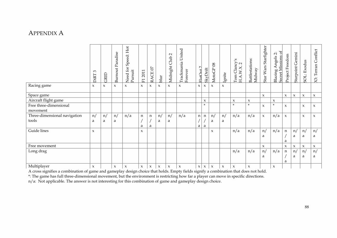
88

APPENDIX A

A cross signifies a combination of game and gameplay design choice that holds. Empty fields signify a combination that does not hold. *: The game has full three-dimensional movement, but the environment is restricting how far a player can move in specific directions. n/a: Not applicable. The answer is not interesting for this combination of game and gameplay design choice.

DiR

T 3

GR

ID

Bu

rno

ut

Pa

rad

ise

Nee

d f

or

Sp

eed

: Ho

t

Pu

rsu

it

F1

20

11

RA

CE

07

blu

r

Mid

nig

ht

Clu

b 2

Tra

ckm

an

ia U

nit

ed

Fo

rev

er

Fla

tOu

t 2

Sk

yD

rift

Mo

toG

P 0

8

Ign

ite

To

m C

lan

cy's

H.A

.W.X

. 2

Ba

ttle

sta

tio

ns:

Mid

way

Sta

r W

ars

Sta

rfig

hte

r

Bla

zin

g A

ng

els

2:

Sec

ret

Mis

sio

ns

of

WW

II

Pro

ject

Fre

edo

m

Sta

rpo

int

Gem

ini

SO

L:

Ex

od

us

X3

: Ter

ran

Co

nfl

ict

Racing game x x x x x x x x x x x x x

Space game x x x x x

Aircraft flight game x x x x

Free three-dimensional movement

* * * x * x x x

Three-dimensional navigation tools

n/a

n/a

n/a

n/a n/a

n/a

n/a

n/a

n/a n/a

n/a

n/a

n/a

n/a n/a x n/a x x x

Guide lines x x x n/a n/a n/a

n/a n/a

n/a

n/a

n/a

Free movement x x x x x

Long drag n/a n/a n/a

n/a n/a

n/a

n/a

n/a

Multiplayer x x x x x x x x x x x x x x x

89