Embed Size (px)
Citation preview

R&D-Based Endogenous Growthin Finland
A Comparative Study on the Semi-Endogenous and
the Schumpeterian Growth Models
Heidi Kaila
University of HelsinkiFaculty of Social SciencesEconomicsMaster’s ThesisMay 2012
brought to you by COREView metadata, citation and similar papers at core.ac.uk
provided by Helsingin yliopiston digitaalinen arkisto

Tiedekunta/Osasto Fakultet/Sektion – Faculty Faculty of Social Sciences
– Department Department of Political and Economic Studies
– Author Heidi Kaila
– Title R&D-Based Endogenous Growth in Finland –A Comparative Study on the Semi-Endogenous and the Schumpeterian Growth Models
– Subject Economics
– Level Master’s Thesis
– Month and year May 2012
– Number of pages 101
– Abstract Theories of endogenous growth aim at finding the sources of productivity growth inside an economy. According to R&D-based endogenous growth theories, total factor productivity (TFP) growth is driven by innovations that improve existing technologies. This thesis studies Finnish TFP growth from 1955 to 2008 by concentrating on two recent theories of R&D-based growth. In the semi-endogenous theory, a steady growth rate of R&D input is required for a sustained TFP growth rate. In the second generation model, also called the Schumpeterian model, a steady level of R&D intensity defined as R&D input adjusted with a measure of product variety, is required for steady TFP growth. These two frameworks are used to analyse a dataset that has been collected and combined from various sources. A nonstationary multivariate time series model (VECM) is used to study the two models in a nested framework which enables the comparison of the models in a robust manner. As far as we know, the nested model approach has not been conducted before in similar empirical studies. The findings of this thesis are that R&D input, using seven different measures, and TFP are cointegrated as suggested by the semi-endogenous model. However, the product variety assumption presented by the Schumpeterian model is not fully rejected although the steady state assumption of strict proportionality between R&D input and product variety is firmly rejected. These findings are in accordance with empirical studies supporting R&D-induced growth in a wider sense. However, they are contradictory with articles that compare semi-endogenous and Schumpeterian models, which have found support for the latter but not for the former. In conclusion, this thesis argues that Finnish TFP has in fact been affected by R&D already when Finland was still lagging behind the world’s high technology frontier.
Avainsanat – Nyckelord – Keywords research and development, productivity, growth theory, time-series analysis
Säilytyspaikka – Förvaringställe – Where deposited
Muita tietoja – Övriga uppgifter – Additional information

Tiedekunta/Osasto Fakultet/Sektion – Faculty Valtiotieteellinen tiedekunta
– Department Politiikan ja talouden tutkimuksen laitos
– Author Heidi Kaila
Työn nimi Arbetets titel – Title T&k-perusteinen kasvu Suomessa –Vertaileva tutkimus semi-endogeenisestä ja Schumpeteriläisestä kasvumallista
– Subject Taloustiede
– Level Pro gradu –tutkielma
– Month and year Toukokuu 2012
– Number of pages 101
Tiivistelmä Referat – Abstract Endogeeniset kasvuteoriat pyrkivät selittämään tuottavuuden kasvua talouden sisällä. T&k-perusteisten kasvuteorioiden mukaan tuottavuuden kasvu syntyy olemassa olevaa teknologiaa parantavista innovaatioista. Tässä tutkimuksessa tarkastellaan Suomen tuottavuuden kasvua vuosina 1955-2008 kahden viimeaikaisen t&k-perusteisen kasvumallin avulla. Semi-endogeenisessa kasvuteoriassa tasaisen tuottavuuden kasvun edellytys steady state -tilanteessa on t&k-panoksen tasainen kasvu. Toisen sukupolven kasvumallissa, jota kutsutaan myös Schumpeteriläiseksi malliksi, tasainen t&k-intensiteetti, eli t&k panos korjattuna tuotteiden moninaisuutta taloudessa kuvaavalla muuttujalla, on edellytys kestävälle tuottavuuden kasvulle. Näitä kahta mallia käytetään analysoitaessa aineistoa, joka on kerätty ja koottu useista lähteistä. Mallien vertailussa käytetään epästationaarista moniuloitteista aikasarjamallia (VECM), joka mahdollistaa kasvumallien vertailun saman aikasarjamallin sisäkkäisinä versioina. Tällaista sisäkkäistä tarkastelua ei ole tiettävästi käytetty aikaisemmin kyseisten kasvumallien vertailussa. Tutkimuksen tulokset osoittavat, että t&k-panos seitsemällä eri muuttujalla mitattuna ja kokonaistuottavuus ovat yhteisintegroituneita semi-endogeenisen mallin osoittamalla tavalla. Tutkimus ei kuitenkaan pysty hylkäämään Schumpeteriläisessä mallissa esiintyvää tuotteiden moninaisuutta kuvaavaa muuttujaa, vaikkakin steady state -oletus t&k-menojen ja tuotteiden moninaisuutta kuvaavan muuttujan välisestä suorasta relaatiosta voidaan hylätä selvästi. Tutkimustulokset ovat yhdenmukaisia t&k-perusteisten kasvumallien empiirisen tutkimuksen kanssa sen laajassa merkityksessä. Ne ovat kuitenkin ristiriidassa semi-endogeenista ja Schumpeteriläistä kasvumallia vertailevien tutkimusten kanssa, joiden tulokset puoltavat Schumpeteriläistä teoriaa. Kaiken kaikkiaan tutkimus osoittaa, että t&k-panoksella on ollut vaikutusta suomalaiseen tuottavuuteen jo pitkän aikaa ennen kuin Suomesta tuli korkean teknologian edelläkävijä.
Avainsanat – Nyckelord – Keywords tutkimus- ja kehittämistoiminta, tuottavuus, kasvuteoriat, aikasarja-analyysi
Säilytyspaikka – Förvaringställe – Where deposited
Muita tietoja – Övriga uppgifter – Additional information

Contents
1 Introduction 6
2 R&D-Based Endogenous Growth Theory 102.1 Microeconomic Foundations . . . . . . . . . . . . . . . . . . . . . . . 10
2.1.1 Rivalry and Excludability . . . . . . . . . . . . . . . . . . . . 112.1.2 Endogenous Growth Theory with "Learning by Doing" and
the AK-model . . . . . . . . . . . . . . . . . . . . . . . . . . . 132.1.3 From Ideas to Technology . . . . . . . . . . . . . . . . . . . . 15
2.2 Models of R&D-Based Endogenous Growth . . . . . . . . . . . . . . . 162.2.1 First generation fully endogenous growth models . . . . . . . . 192.2.2 The Semi-Endogenous Growth Model . . . . . . . . . . . . . . 232.2.3 Second Generation Fully Endogenous Growth
Model or Schumpeterian Growth Model . . . . . . . . . . . . 282.3 Technology Transfers . . . . . . . . . . . . . . . . . . . . . . . . . . . 34
3 Data 373.1 Output, Labour and Total Factor
Productivity . . . . . . . . . . . . . . . . . . . . . . . . . . . . . . . . 373.2 R&D Input Variables . . . . . . . . . . . . . . . . . . . . . . . . . . . 403.3 Variables Indicating Semi-endogenous
R&D Input . . . . . . . . . . . . . . . . . . . . . . . . . . . . . . . . 433.4 Variables Indicating Schumpeterian R&D Intensity . . . . . . . . . . 46
1
4 Econometric Methods: Vector Autoregressive and Vector ErrorCorrection Models 50
5 Results 585.1 Estimation Equation . . . . . . . . . . . . . . . . . . . . . . . . . . . 585.2 Cointegration Test of the Unrestricted
Model . . . . . . . . . . . . . . . . . . . . . . . . . . . . . . . . . . . 615.3 Cointegration Test of the Semi-Endogenous Model . . . . . . . . . . . 655.4 Cointegration Test of the Schumpeterian Model . . . . . . . . . . . . 695.5 Discussion . . . . . . . . . . . . . . . . . . . . . . . . . . . . . . . . . 71
5.5.1 Comparison with International Literature . . . . . . . . . . . 715.5.2 Studies on Finnish Productivity . . . . . . . . . . . . . . . . . 765.5.3 Discussing the Steady State and Final Remarks . . . . . . . . 79
6 Conclusions 85
A Empirical Variables 87
B Unit Root Tests 88
C Residual Diagnostics 89
D SITC-classifications 92
References 94
2

List of Figures
3.1 GDP and labour (indexed) . . . . . . . . . . . . . . . . . . . . . . . . 383.2 Left: TFP (log), right: TFP growth rate. . . . . . . . . . . . . . . . . 403.3 Combining the patent data up left: solid: Number of patent appli-
cations by office, dash: Number of patent applications by countryof origin. Up right: solid: Number of patent grants by office, dash:Number of patent grants by country of origin. . . . . . . . . . . . . . 42
3.4 Variables indicating R&D input plotted with TFP (all variables areindexed for the graph). . . . . . . . . . . . . . . . . . . . . . . . . . . 45
3.5 Variables indicating growth of R&D input. . . . . . . . . . . . . . . . 463.6 Variables indicating R&D intensity X/Q. . . . . . . . . . . . . . . . . 49
5.1 The cointegrating residuals of the unrestricted models with R&D ex-penditures, productivity adjusted R&D expenditures and high tech-nology imports. . . . . . . . . . . . . . . . . . . . . . . . . . . . . . . 63
5.2 The cointegrating residuals of the unrestricted models with patentapplications and patent grants. . . . . . . . . . . . . . . . . . . . . . 64
5.3 The cointegrating residuals of the unrestricted models with R&Dworkforce and R&D person-years. . . . . . . . . . . . . . . . . . . . . 65
5.4 Cointegration residuals of the semi-endogenous model, up left: Hightechnology imports & labour, up right: Patent applications & output,down: Patent grants & labour. . . . . . . . . . . . . . . . . . . . . . . 67
3

5.5 Cointegration residuals of the semi-endogenous model, left: Produc-tivity adjusted R&D-expenditures & labour, right: R&D person-years& output. . . . . . . . . . . . . . . . . . . . . . . . . . . . . . . . . . 68
5.6 The cointegrating residual of the model with patent applications andoutput. . . . . . . . . . . . . . . . . . . . . . . . . . . . . . . . . . . . 70
4

List of Tables
5.1 The unrestricted model (Johansen approach) . . . . . . . . . . . . . . 825.2 Critical values of the trace-test . . . . . . . . . . . . . . . . . . . . . 835.3 The semi-endogenous model (S2S approach) . . . . . . . . . . . . . . 835.4 The Schumpeterian model (S2S approach) . . . . . . . . . . . . . . . 84
B.1 Unit root tests . . . . . . . . . . . . . . . . . . . . . . . . . . . . . . 88
C.1 Residuals of the VAR model . . . . . . . . . . . . . . . . . . . . . . . 89C.2 Residuals of the unrestricted model (Johansen approach) . . . . . . . 90C.3 Residuals of the semi-endogenous model . . . . . . . . . . . . . . . . 91C.4 Residuals of the Schumpeterian model . . . . . . . . . . . . . . . . . 91
5

Chapter 1
Introduction
In the classical growth model by Solow (1956), technology is "manna from heaven"and enters the production function as an exogenous variable; growth resulting fromother factors than capital or labour is unexplained. Endogenous growth theory aimsto represent technology as an endogenous variable in the production function, sothat one can understand exactly how technology is invented.
In this study we show that R&D and TFP have had a strong relation in Finlandalready since the 1950’s. Our study is motivated by an article by Jalava et al. (2002),"Technology and Structural Change: Productivity in the Finnish Manufacturing In-dustries, 1925–2000". The authors leave an important question to be answered byfuture research: "Why has the TFP growth been so strong in the Finnish manu-facturing industries?" This thesis studies Finnish TFP as an aggregate, but surelya great part of the growth can be traced down to the manufacturing sector.1 It isclear that technological change particularly in ICT has been the driver of growthin Finland from the 1990’s, but it is not so evident what kind of role research anddevelopment has played earlier.
This study suggests that for the period 1955–2008, research and development,measured with several different indicators, has had an impact on the growth of
1Over 50% of Finnish productivity growth resulted from the manufacturing sector during 2000–2005 (OECD 2006).
6

Finnish TFP. We have studied two front-line theories of endogenous growth, thesemi-endogenous and the Schumpeterian growth models, to study two possible ex-planations of the nature of the relation between R&D and TFP.
Contradictory to the findings of several prominent articles,2 we found out that thesemi-endogenous model describes well the Finnish economy. The semi-endogenoustheory claims that a steady growth rate of R&D input is required for a sustainedTFP growth rate. Indeed, Finnish R&D input and TFP growth are cointegratedand move "hand-in-hand", even though TFP growth has been much faster than thegrowth of any of the R&D inputs studied.
The Schumpeterian model states that a steady level of R&D intensity, definedas R&D input adjusted with a measure of product variety, is required for steadyTFP growth. We cannot reject the hypothesis that product variety –the notionthat as the economy grows, innovations are diluted over a larger number of sectors–plays some kind of role in Finnish TFP growth. Nevertheless, the steady stateproperty of product variety, namely that R&D input and product variety growstrictly proportionately together, is firmly rejected.
In this study, a generalized version of a productivity-growth function presentedby Ha & Howitt (2007), is estimated inside a nonstationary multivariate time seriesmodel. Contradictory to previous studies that have estimated two separately definedmodels,3 in this study the semi-endogenous and Schumpeterian models are estimatedas nested models inside a VECM-framework. This sort of statistical specificationof the models gives formally comparable results, since in addition to setting thehypothesis for the validation of the model in question, also the hypothesis of rejectingthe competing model can be tested simultaneously.
Our dataset has been collected and combined from various resources, also partlyfrom non-digital sources. The time span of the study, 1955–2008, is longer than inmany other studies of Finnish productivity which mostly concentrate on the ICT
2For example Ha & Howitt (2007), Madsen (2008), Madsen et al. (2010), Zachariadis (2003)and Zachariadis (2004).
3For example Ha & Howitt (2007) and Madsen et al. (2010).
7

-era. Therefore this study provides valuable insight to the Finnish success storyalready after World War II, finding out that not only has R&D been importantfor the new Nokia -economy, but that it already played a significant role duringthe times when Finland was in European terms a backward economy, growth wasdriven by Soviet trade, wood, paper and metal being the cornerstones of the economy(Hjerppe 2008).
Empirical studies on endogenous growth have generally concentrated on largeeconomic entities, such as the U.S. and G5 countries (Jones 1995a; Ha & Howitt2007) or OECD countries (Coe et al. 2009), since endogenous growth theories aretypically seen as describing a larger entity than a national economy, due to thenonrival nature of ideas. However, as a recent study by Pessoa (2010) shows, therelation between R&D and economic growth differs largely from country to country.Therefore, we regard that a country-level setting, when the effects of foreign R&Dare also taken into consideration, presents a fresh way of using the R&D-basedgrowth theories. We are not the first to collaborate this idea though; a study onIndia by Madsen et al. (2010) finds positive results on the effects of both foreignand domestic R&D to TFP growth.
The thesis is constructed as follows: The theoretical frameworks are presentedin chapter 2 starting with the microeconomic foundations of endogenous growththeory in chapter 2.1. The R&D-based growth models are discussed in chapter2.2. We follow the theoretical framework by Ha & Howitt (2007), presenting themodels in historical order. First we study the first generation fully endogenousgrowth models by Romer (1990), Aghion & Howitt (1992) and Grossman & Helpman(1991), then the semi-endogenous growth models by Jones (1995b), Kortum (1997),and Segerström (1998) and finally, the second-generation or Schumpeterian fullyendogenous growth models by Aghion & Howitt (1998), Howitt (1999), Dinopoulos& Thompson (1998) and Young (1998).
In the empirical part of the study chapter 3 describes the collecting and combin-ing of the data and some observations concerning it. The methods of multivariate
8

time series analysis are presented in chapter 4, and finally the estimation of themodels is done in chapter 5, where in section 5.5 we discuss our results comparingthem with previous research. Lastly, chapter 6 concludes and presents ideas forfurther research.
9
Chapter 2
R&D-Based Endogenous GrowthTheory
In this chapter we first present the microeconomic foundations of endogenous growthmodels on a general level, including a short side-step to the endogenous growthmodels that build on capital instead of R&D. Then we move onto the macroeconomicmodels studying the first generation, the semi-endogenous and the second generationgrowth models. Finally, we take a short look on how technology transfers affect TFPgrowth.
2.1 Microeconomic Foundations
Research and development is about producing ideas and inventions. Firstly, in orderto understand the special nature of producing ideas or knowledge, we introduce theconcepts of rivalry and excludability following Romer (1990). Secondly, we brieflydescribe some endogenous models that are not based on R&D, but which connectproductivity with capital accumulation.
Finally, we move towards to the R&D-based macroeconomic models. The modelintroduced by Romer (1990) is regarded as being the foundation stone for all the
10

R&D based growth models, not least because of its solid microeconomic framework.We briefly describe the model as an example on how an optimal R&D input isderived inside a microeconomic framework.
2.1.1 Rivalry and Excludability
According to Romer (1990) "a purely rival good has the property that its use by onefirm or person precludes its use by another; a purely nonrival good has the propertythat its use by one firm or person in no way limits its use by another".
Ideas are thus nonrival: the use of an idea in a certain activity does not limitthe use of the same idea in another activity. A good example of a perfectly nonrivalgood is calculus. Romer defines rivalry and excludability as technological attributesof goods, but excludability can also be achieved through the legal system. Exclud-ability means that the owner of a good can exclude others from using it (Romer1990). In idea-based products an excludable good could be a satellite-tv and annonexcludable good the results of basic research.
Conventional economic goods that can be privately owned and traded in com-petitive markets are both rivalrous and excludable (Romer 1990). Nonexcludablegoods that are also nonrival are called public goods (for example national defenseand scientific research). The degree of excludability can be expressed as an ex-ternality. Nonexcludable goods that have positive externalities are often publiclyproduced and a perfectly nonexcludable good cannot be privately traded in markets(Romer 1990).
Rivalry and excludability are linked: a rival good generally is also excludablesince owning a rival product means that one can exclude others from using it (Romer1990). An exception to the rule is a good that suffers from "tragedy of the commons"problem, from the inability to define the ownership of the good. For instance fishin the sea are indeed rival but still nonexcludable.
However, excludability does not imply rivalry. Technology as a nonrival goodcan be excludable: for example a design produced in a private, profit-maximizing
11

company is rival, but the firm can control its copying and therefore the firm canalso sell the idea.
Romer also highlights the difference between human capital and "ideas" as goodsthat can be nonrival and nonexcludable: A piece of human capital, say the knowledgeof calculus, is tied to a human body and thus it can only be used once at a timewhich makes the knowledge of calculus both rival an nonexcludable, whereas calculusitself is a nonrival and nonexcludable good. Human capital can therefore be tradedin competitive markets whereas the underlying nonrival and nonexcludable ideascannot.
Perfect nonrivalry is an idealization, since the idea is itself tied to somethingphysical, like on a computer. Thus its copying is not free, but the marginal costsare much smaller than the fixed costs that are related to producing the idea in thefirst place. Hence there are increasing returns to scale in the production of ideasor "idea-intensive" goods (that can be rival), that use nonrival goods as inputs. Bydoubling the costs of production (the input) of a certain amount of goods more thandoubles the amount of final goods produced (the output). Because of the fixed costs,also labour productivity rises with the scale of production of the final good (Romer1990).
Formally, a production function F that uses a nonrival input A and a rivalinput X cannot be concave because F (λA, λX) > λF (A,X). More generally, sinceF (A,X) = X dF
dX(A,X), it follows that F (A,X) < AdF
dA(A,X) + dF
dX(A,X). If all
inputs are paid their value marginal product, the firm suffers losses (Romer 1990).Since in perfect competition the price of the final product will be equal to marginalcost, the firm will make a loss equal to the fixed costs (Romer 1990).
This result means that in a market where inputs used are nonrival, perfect com-petition is impossible and imperfect competition is a necessary condition for thismarket to exist. A monopolist producer can reduce production and set the price tobe equal to the marginal revenue.
The monopoly power can be guaranteed by giving a right (a patent for instance)
12

that makes competition impossible. From the point of view of the social optimum,the result is similar to any other monopoly market: the product is underused andthere is a dead weight loss (Romer 1990).
2.1.2 Endogenous Growth Theory with "Learning by Do-
ing" and the AK-model
The common idea in the "learning by doing" and the AK-models is that capitalaccumulation –whether it is physical or intangible capital– results in productivitygrowth. The "learning by doing" model of Arrow (1962) formulates this so that extraphysical capital necessarily leads to an equiproportionate increase in knowledge whenworkers learn to use the new capital. In the AK-models by Romer (1986), Romer(1987), Lucas (1988) and Rebelo (1991), investment in broadly defined capital hasa positive long-run effect on growth. For instance Lucas (1988) formulates a modelwhere the production of human capital generates knowledge, which is a nonrival,nonexcludable good.
Arrow (1962) formulates the issue of "learning by doing" through an individualcompany that takes extra capital into use (taking it as given). Solving the modelyields constant returns at the firm level, but increasing returns to scale at the aggre-gate level. The growth at the aggregate level comes not just from the direct effectof having additional aggregate capital, but moreover from workers having to learnto use the new capital and thus becoming more sophisticated. The firm that hasincreased its capital stock does not collect the profits, since other firms will imitateit and workers will spread the knowledge in the long run by changing their employer.Thus there is an externality: "a knowledge spillover" that results in technologicaladvancement.
In the AK-model there is also an externality from additional capital, so thatcapital enters the production function as technology.4 In the AK-model there is an
4A simple generalization of the AK-model describes well the idea: Technology is now defined asAt = Kφ
t = Kt, where φ = 1. The aggregate production function becomes Yt = Kαt (KtLt)1−α =
13

infinite or very long time for convergence to the steady state. As in learning bydoing, there are increasing returns to scale in capital at the aggregate level.
The important result arising from the AK-model is that a higher savings rate (orrate of accumulation of human capital) gives rise to a permanently higher growth rateof GDP. However, an increasing population also affects the growth rate of outputpositively, meaning there is a scale effect that is contradictory to empirical findings(the scale effect is discussed in detail in chapter 2.2).
Romer (1990) criticizes "learning by doing" because of the "strict proportionalitybetween knowledge and physical capital or knowledge and education as an unex-plained and exogenously given feature of the technology", and because it neglectsthe possibility that firms intentionally make investments in R&D. In "learning bydoing" the production of a nonrival, nonexcludable good is only an unintentionalside effect of the production of a conventional good.
By studying investment shares, Jones (1995a) concludes that the AK-models donot provide a good description of the driving forces behind growth in developedcountries. The evidence suggests that there are effects from the increasing savingsrate, but that they are transitory, not permanent like the AK-model suggests. Apercentage point increase in the investment rate results in growth increasing for fiveto eight years.
However limiting might these theories might seem, they are still valid to someextinct. Bernanke & Gürkaynak (2001) present evidence that the rate of investmentin human capital is a statistically significant factor in explaining labour productivitygrowth. Also Jones (1995a) claims that the evidence against the AK-model is notas strong as the evidence against the first generation models (presented in chapter2.2.1).
KtL1−αt where now L1−α
t is denoted by A, which is a constant. This is inconvenient, but it explainswhere the name "AK-model" comes from.
14

2.1.3 From Ideas to Technology
The Romer model is a good example on how endogenous growth models are usuallyconnected to microeconomic theory. Romer (1990) presents a model which has threesectors in the economy. The research sector uses human capital and the existingstock of knowledge to produce –as Romer puts it– designs, meaning new knowledgeor ideas, for new producer durables (intermediate goods). An intermediate-goodssector uses these designs to produce the producer durables that are available foruse in final goods production. A final goods sector uses these producer durablesas well as labour and human capital to produce final output. The monopolisticcompetition enters the model so that the research sector obtains a patent on the useof the design in the production of the intermediate good that the design supports,and then transfers the patent (by leasing or selling) to the intermediate sector. Themarket for each design is a monopoly where the supplier sets the price (Romer 1990).Inside this microeconomic framework, the optimal share of the labour force workingfor the R&D -sector (research share) that maximizes the growth rate of GDP perworker, can be derived.
Note that technology is productive in two ways, in the final goods sector thatuses the intermediate goods produced with the new designs, and also in the researchsector where the existing stock of knowledge is used in producing new designs. Thismeans that even though there is a patent related to all the designs, the knowledgeembodied in the design may be detectable and of use in the whole research sector.In this way the nonrival nature of ideas is present in the model (Romer 1990).
In several theories of R&D-based growth, a model with multiple sectors (onebeing the R&D sector) is introduced in a similar manner and an optimal R&Dinput, or share of R&D workforce, is derived. For example Aghion & Howitt (1992),Grossman & Helpman (1991), Jones (1995b) and Howitt (1999) all present theirown variety of this kind of sectoral framework.
The fact that all these articles explicitly state that they are building on a sim-ilar framework introduced by Romer (1990) is the reason why we have chosen to
15

introduce specifically the Romer-model to describe this microeconomic framework.
2.2 Models of R&D-Based Endogenous Growth
The underlying idea in R&D-based endogenous growth theories is that R&D hasan impact on TFP growth. Productivity can thus be influenced by economic pol-icy: institutions and regulations create incentives to innovate which result in newtechnologies (Ha & Howitt 2007). There are several theories which aim at explain-ing how productivity and technology are affected by R&D. Ha & Howitt (2007)present a general form of productivity-growth function, which can be used to sep-arate between different theories of R&D-based endogenous growth. These can begrouped in to three categories which are (in historical order) first generation fullyendogenous growth models, semi-endogenous growth models and second generationfully endogenous growth models (which Ha & Howitt refer to as the Schumpeterianmodel).
Like Ha & Howitt (2007), we also estimate only the most recent models, thesemi-endogenous and the second generation models. The first generation modelsare left out of estimation since there already exists substantial evidence refutingthem, and since the later theories are particularly developed in order to respond tothese inaccuracies.
However, first generation models are, like the name suggests, the first attempts toexplain growth arising from R&D. Thus they lay the foundation for the succeedingtheories, a reason why we still include them in the theoretical part of the thesis. Wediscuss the empirical evidence against the first generation models together with thetheory in chapter 2.2.1, but the empirical evidence of the semi-endogenous and thesecond generation model is left to the discussion in chapter 5.5, in order to comparethe literature with our results.
Ha & Howitt (2007) define the general form of a productivity-growth functionas
16

(2.1) gA = λ
(X
Q
)σAφ−1,
where in steady state
(2.2) Q ∝ Lβ.
Then equivalently, the "ideas production function" or knowledge creation functionis defined as5
(2.3) A = λ
(X
Q
)σAφ.
X is defined as R&D input (or productivity adjusted R&D input), A is technol-ogy (TFP) and Q is product variety.
Parameter σ defines the effect of R&D input (σ > 0)6 (Ha & Howitt 2007). Theeconomic interpretation of the parameter is that if σ < 1 there will be duplicationof ideas or "stepping on toes" -effect, which affects negatively the production oftechnology. This means that there is a negative externality from the use of R&Dinput, meaning that the more firms there is at the R&D -sector, the more probableit is that their work overlaps resulting from not having perfect knowledge on eachother’s results. If σ = 1, there is no effect like this. Empirically R&D input X isoften measured by the number of researchers in the R&D sector, real expendituresin R&D or the number of patents. It is also very common to use the share of labourforce working for the R&D sector as R&D input.
5since gA = A/A
6By imposing restriction σ = 0 we get TFP growth of the neo-classical model, where there isno R&D input. We do not study this case.
17
Parameter φ defines the returns to scale in knowledge (φ ≤ 1).7 If φ > 0, themore there are ideas produced in the past, the more productive are the new ideas.8
This is called the "standing on shoulders" -effect and it is often claimed that theright value for φ is either close to one or smaller than one. If φ < 0, then it ismore and more difficult to produce new ideas, because the easiest ideas are alreadyinvented. This is called the "fishing out" -effect.9 The case of φ = 0 means thatthe effects are equally big; productivity of ideas is independent of its history (Jones1995b).
In steady state, product variety Q is proportional to the size of the labour force.Lβ is thus empirically used for approximating product variety, parameter β is definedas product proliferation (β = 0 or β = 1).10
Using the share of labour working in research and development as R&D inputhas been very common in the literature of R&D-based endogenous growth. Ha &Howitt (2007) study equation 2.1 also in this special case so that X = N = νL,where N is the number of workers in R&D expressed as fraction ν of labour, whichis assumed to be constant in steady state and as previously, Q = Lβ.
With this specification equation 2.1 becomes11
(2.4) gA = λ(νL1−β
)σAφ−1.
This special case has important implications to growth in the three differentmodels and will be discussed later in this chapter.
7For instance, if ideas are produced by R&D workers LA at a rate λ (and there is no productvariety in the model), the knowledge creation function is A = λLσA where λ = λAφ so the rate λdepends on the stock of ideas already invented (Jones 1995b). By combining these two equationsthe production function for ideas can be expressed as A = λAφLσA.
8λ is increasing in A.9λ is decreasing in A.
10Product variety Q and parameter β are only present in the Schumpeterian model which isexplained more thoroughly in chapter 2.2.3.
11By replacing X with νL and Q with Lβ we get gA = λ(νL/Lβ)σAφ−1.
18

2.2.1 First generation fully endogenous growth models
The first R&D-based endogenous growth models were developed by Aghion & Howitt(1992), Grossman & Helpman (1991) and Romer (1990). Ha & Howitt (2007) gen-eralize the productivity-growth function in these models to be
(2.5) gA = λXσ,
where parameters are restricted so that φ = 1, 0 < σ ≤ 1 and β = 0 (so thatboth A and Q vanish from the equation 2.1). Parameter σ is slightly more restrictedin these models than in the semi-endogenous and Schumpeterian models, but as Ha& Howitt (2007) state, the restriction is not crucial in distinguishing between themodels.
Equivalently, the knowledge-creation function or ideas production function is
(2.6) A = δXσA.
In Ha & Howitt (2007), the R&D input X is specified as either the flow of R&Dlabour N , or the productivity-adjusted flow R/A of R&D expenditure. However, inthe original models of Aghion & Howitt (1992), Grossman & Helpman (1991) andRomer (1990), R&D labour was regarded as the most important input in R&D, sinceresearch is labour intensive work. This however resulted in a scale effect, a distinctivefeature of all the first generation theories, implying that a larger population shouldresult in higher GDP growth, thus the scale of the population matters for growth.This result is contradictory to empirics, since the development in the 20th centuryhas been of a declining population growth with a steady growth in GDP.
The scale effect can be seen by modifying equation 2.4. For the first generationmodels with parameter restrictions defined above, this reduces to
19

(2.7) gA = λ (νL)σ .
Thus growth depends on the level of both the research share ν and labour L (Ha& Howitt 2007).
In an original model by Romer (1990) (which can also be regarded as presentingan AK-model as previously noted), human capital is the R&D input.12 The scaleeffect is therefore present in this model, since human capital is tied to labour force.
Romer (1990) explains the scale effect so that a larger population means a largermarket for ideas. Due to the nonrival and nonexcludable nature of ideas, the pro-duction of ideas has increasing returns to scale and therefore ideas can easily crossborders. Romer (1990) sees that therefore also the benefits can be taken into usein a larger area with relatively very little costs. As Romer puts it, "increases in thesize of the market have effects not only on the level of income and welfare, but alsoon the rate of growth. Larger markets induce more research and faster growth".
The parameter restriction φ = 1 in equation 2.6 is a feature that distinguishesthe first generation models from the semi-endogenous models. This assumption im-poses constant returns to knowledge in the production of new knowledge. In Aghion& Howitt (1992), where they present a very similar ideas production function as Ha& Howitt (2007), this follows from the assumption that each innovation producesa fixed proportional quality improvement. In the product-variety model of Romer(1990), constant returns arise from a special assumption on the knowledge spilloveraccording to which an increase in the number of existing varieties facilitates thegeneration of new varieties. In Grossman & Helpman (1991) constant returns in
12The ideas production function of Romer is very similar A = λHAA, where HA is total humancapital employed in research and λ is the productivity parameter. Having the exponent of HA
fixed to 1 is not a crucial assumption, but Romer claims that it imposes linearity in HA, becauseweakening this assumption would require a more detailed specification of how income in the researchsector is allocated to the participants. Romer claims that it is not important for the dynamicproperties of the model (Romer 1990).
20

innovative activity is present in modelling the growth of consumers’ utility. Accord-ing to Ha & Howitt (2007), constant returns is what allows sustained, non-explosivegrowth.
What is distinctive in Grossman & Helpman (1991) is the notion of productinnovation being horizontal and vertical, horizontal meaning differentiated products(increasing the product variety) and vertical meaning the quality improvement of analready existing product. Thus they take into account the "increasing complexity"through horizontal differentiation.13
The microfoundations are quite similar in the models of Romer (1990) andAghion & Howitt (1992). However, a completely novel factor in Aghion & Howitt(1992) is the notion of "creative destruction". In Aghion & Howitt (1992), creativedestruction means that there is a factor of obsolescence: when new products arrivethey render previous products obsolete. This progress creates both gains and lossesin growth. The underlying idea of creative destruction comes from Schumpeter(1942):
The fundamental impulse that sets and keeps the capitalist engine in motioncomes from the new consumers’ goods, the new methods of production or transporta-tion, the new markets,.... [This process] incessantly revolutionizes the economicstructure from within, incessantly destroying the old one, incessantly creating a newone. This process of Creative Destruction is the essential fact about capitalism.
Based on this idea, Aghion & Howitt (1992) assume that individual innovationscan be powerful enough to affect the entire economy. The length of innovatingtime is random due to the innovations arrival rate being a stochastic process, butthe relationship between the amount of research in two successive periods can bemodelled as deterministic.
In the model of Aghion & Howitt (1992) there are two effects arising from thenotion of creative destruction, through which the amount of research this period
13It is not formally analogous to the way in which in the second generation model (Ha & Howitt2007) deflate X by L, but it has a similar underlying idea.
21

depends negatively upon the expected amount of research next period. The firstone is that the pay-off from research this period is the prospect of monopoly rentsnext period, which will last until the next innovation arrives. The mechanism behindthis idea is that research is assumed to produce a random sequence of innovations.The arrival rate of innovations is a Poisson-process which has the property thateach innovation occurs independently of the time since the last occurrence. Theexpected present value of the rent depends negatively on the Poisson arrival rate ofthe next innovation. This Poisson arrival rate (or the rate of creative destruction)of innovations in the economy at any given moment is defined as
(2.8) λφ(nt+1).
Here λ is the arrival parameter, φ a constant-returns, concave production func-tion and n is the flow of researchers (the input in innovation production). Technologyof research determines parameters λ and φ, thus the arrival rate depends only uponthe current flow of inputs to research.
The second effect of creative destruction is connected with the labour marketequilibrium. The result is that higher expected research next period is connectedwith less innovative activity today. The rational is that since labour can be allocatedeither to research or to some other activity, the expectation of more research nextperiod corresponds to a higher demand of researchers in the next period, and there-fore higher real wage of researchers. This decreases monopoly rents and thereforediscourages research this period.
Finally, GDP growth in this model is a function of the size of innovations, theamount of researchers, and the productivity of research as measured by a parameterindicating the effect of research on the Poisson arrival rate of innovations.
As noted before, the first generation model models suggest that a larger numberof R&D workers or a larger share of R&D workers of the labour force results in an
22

increasing growth rate of TFP. However, on the long run, the research share has hada positive growth trend, but the output growth as well as TFP growth rates havebeen stationary and trendless (Jones 1995a; 1995b). Jones argues that increasinglevels of the number of researchers and engineers and certain other policy variables(Jones refers to for example human capital -related variables, export shares, propertyrights etc.) has not resulted in an increase in output nor TFP growth. Jones claimsthat the movements of explanatory variables have been large and persistent duringthe postwar era whereas movements in output and TFP growth have little or nopersistent increase. In fact, according to Jones (1995a), the growth rates of 14OECD countries and the U.S. have all been stationary. Simultaneously however,the number of R&D workers as well as their share of the labour force has grownsignificantly, for instance in the U.S. the share of scientists and engineers of thelabour force grew threefold from 1950 to 1988, from 0.25% to nearly 0.8%. Thisevidence clearly speaks in favour of refuting the first generation models.
2.2.2 The Semi-Endogenous Growth Model
The semi-endogenous growth model was first introduced by Jones (1995b) and con-tinued by Kortum (1997) and Segerström (1998). The growth rate of TFP in thesemi-endogenous model is
(2.9) gA = λAφ−1Xσ
(Ha & Howitt 2007; Jones 1995b), where σ < 1 and φ < 1. We can see thatwhen At goes to infinity, Aφ−1
t approaches zero and the growth rate has to fall. Notethat there is no product variety variable Q in the model, parameter β in equation2.2 is set to zero.
Even though Ha & Howitt (2007) generalize the first generation articles to haveσ < 1, Jones (1995b) as a matter of fact sees that σ = 1 is a common feature
23
in the first generation models.14 As we noted previously, Romer (1990) has madethis restriction and in fact, also Aghion & Howitt (1992) assume constant returnsproduction function for the flow of R&D input, which means that TFP growth isproportional to the share of R&D workers, meaning proportional to the size of thelabour force in steady state. In his article, Jones (1995b) introduces, to his view forthe first time, the possibility of σ < 1, in order to have decreasing returns to scalein research input.
Whatever is the right way to generalize first generation models, it is true thatthe semi-endogenous model has σ < 1 in the production function of ideas. In fact,the true novelty of the theory lies in another parameter restriction, in the semi-endogenous model it is assumed that φ < 1, which introduces a new way of thinkinghow the arrival rate of innovations depends less strongly on the existing stock ofknowledge.
Therefore what is common to the models of Jones (1995b), Kortum (1997) andSegerström (1998) is the thought that the most obvious ideas are discovered first, sothat the probability that a person engaged in R&D discovers a new idea is decreasingin the level of knowledge.
Kortum (1997) and Segerström (1998) are very sure on this "fishing out" -effectto exist in knowledge production (φ < 0), but Jones (1995b) allows, in his view, forboth decreasing and increasing returns to scale, (φ < 1) since he sees that φ > 0,represents increasing returns to scale in knowledge production. Therefore he regardsas φ = 0 a benchmark of constant returns to scale (zero external returns) in whichthe arrival rate of new ideas is independent of the stock of knowledge.
This is contradictory to how the first and the second generation theorists seethis parametrization, as they regard the case φ = 1 implying constant returns toknowledge. Jones considers that already having previous discoveries in the ideas pro-
14Jones calls this group of models "Romer/Grossman-Helpman/Aghion-Howitt -models" referringto Romer (1990), Aghion & Howitt (1992) and Grossman & Helpman (1991a, 1991b and 1991c).So Jones refers to very much the same literature that Ha & Howitt (2007) which they call the firstgeneration.
24

duction function refers to increasing returns (φ > 0) and first and second generationtheorists see it as a natural input in the production function.15
It is noteworthy that the effect of φ is external to the scientist; it measures thedegree of externalities across time in the R&D process. As a matter of fact, Jones(1995b) argues that the question of the returns to scale in innovation is rather aphilosophical question. Jones criticizes the first generation theorists from imposingtoo strict restrictions by setting φ = 1, and claims that it represents a very arbitrarydegree of increasing returns. In fact, the benefit of this parametrization is that itproduces a model that is "fully endogenous" which is often seen as an end itself. Inspite of having criticized the first-generation theorists for setting arbitrary parameterrestrictions, Jones (1995b) does the same by imposing the restriction φ < 1, which,albeit being less restrictive, has also the purely theoretical advantage that it allowsthe economy to move towards a balanced growth path. So when φ really is close toone, then the speed of convergence to the steady state becomes slower.
Another common feature of the semi-endogenous models (Jones 1995b; Kortum1997; Segerström 1998) is that they suffer from the scale effect; growth in steadystate is ultimately tied to population growth. Ha & Howitt (2007) explain thisproblem by studying the change of the growth rate in equation 2.9. By taking logsand differentiating with respect to time, the growth equation becomes16
(2.10) gAgA
= (1− φ)((
σ
1− φ
)gX − gA
),
where gX is the growth rate of R&D input.17
15In these articles the discussion of the returns to scale is rarely formulated mathematically soit is not always clear whether the authors speak of the knowledge production function as a wholeor only the returns to scale to the existing stock of knowledge. To our view the increasing returnsto production as a whole would mean that σ + φ > 1 and increasing returns to only the existingstock of knowledge A would mean φ > 1.
16Using the approximation that for a certain variable a, the growth rate can be defined asga = ∆ ln at = ln at − ln at−1 ≈ d ln at/dt .
17By taking logs the equation 2.9 becomes ln gA = lnλ + σ lnXt + (φ − 1) lnAt and then by
25
In balanced growth the change of the growth rate of A is zero (growth is con-stant). Therefore by replacing this to the left-hand-side of equation 2.10, we getσgX − (1− φ)gA = 0, so in steady state
(2.11) gA = σ
1− φgX .
Thus with time, productivity growth rate approaches the growth rate of R&Dinput (if gX is constant or approaches a constant).
The scale effect rising from this result can be seen more explicitly if we study theshare of R&D workers as the research input. By replacing X with νL in equation2.9, the growth rate becomes
(2.12) gA = λ (νL)σ Aφ−1.
If we assume like Ha & Howitt (2007), that in a balanced growth path thegrowth of ν cannot exceed population growth n, we can say that in this settingthe growth rate gA will converge to ( σ
1−φ)n. Then in the balanced growth path thefraction of resources devoted to R&D does not matter, policies to stimulate R&D hasmostly transitory effects. Jones (1995b) sees that the scale effect means that whenthe world population grows, the number of researcher grows and these researchersproduce more ideas, which raise incomes around the world (Jones 1995a).
Jones (2002) presents some empirical evidence to support his theory of semi-endogenous growth. Contradicting the conventional view that the steady growthrate of the U.S. output over a period of 125 years has indicated the economy beingclose to its long-run steady-state balanced growth, Jones claims instead that theeconomy has been in a period of transitional growth, but that this growth has been
taking a time derivative using the approximation the equation becomes d ln gAt/dt = σ(lnXt −lnXt−1) + (φ− 1)(lnAt − lnAt−1) which can be formulated as equation 2.10.
26

constant. Jones calls it the constant growth path.Jones (2002) presents two changes that have occurred during the last 50 years to
justify his claim. First, time spent accumulating skills through education (human-capital investment) has increased substantially and second, the research share ofR&D workers of total labour force has increased. In theory, these kinds of changesshould generate transition dynamics in the short run, creating a temporary rise inthe growth rate, and "level effects" in the long run, referring to a permanently higherlevel of output in the new steady state.
According to Jones (2002), the growth rate can be constant even outside thebalanced growth path, since the accumulation of human capital and increase inresearch share have been steady for the last 50 years.
Through a growth accounting exercise of the growth rate of U.S. output overthe period 1950 to 1993, Jones (2002) suggests that more than 80 percent of growthwas associated with transition dynamics: The rising level of educational attainmentaccounts for over one-third of growth and increasing share of R&D workforce in theG5 countries accounts for about 50 percent of growth. Only 10 to 20 percent is dueto the long-run component, which in the semi-endogenous model is the increasingpopulation (Jones uses the population of G5 countries as a measure).
Jones claims that the relevant scale variable is the population of the collectionof countries that are sufficiently close to the world’s technological frontier, that theycan contribute to the discovery of new ideas (Jones considers population of the G5countries a good proxy). So for an individual country, it is the scale of world researcheffort that matters for the economic performance.
Jones (2002) also argues that the semi-endogenous theory is not contradictingcross-country growth regressions that generally have found a negative correlation be-tween per capita output growth and population growth. This is true in the model’ssteady state, but outside the steady state (in the constant growth path); a higherpopulation growth rate reduces the steady-state capital-output ratio because moreinvestment must go simply to maintain the existing capital-output ratio of the grow-
27

ing population.Jones (2002) acknowledges the fact that inside his model the growth cannot
continue forever. If human capital accumulation and the increase in the researchshare cease, the growth rate will fall. According to Ha & Howitt (2007), the resultthat R&D policies do not affect the steady state growth rate, is a crucial flaw in themodel.
2.2.3 Second Generation Fully Endogenous Growth
Model or Schumpeterian Growth Model
The common feature to pre-second generation R&D-based endogenous growth mod-els is the fact that as the population rises, so do the rate of technological progressand the growth rate of output per person. This is a result from the scale effect causedby the nonrival and nonexcludable nature of innovations (favouring a large market)and from the larger supply of potential R&D workers (Howitt 1999). The secondgeneration fully endogenous growth theories by Aghion & Howitt (1998, ch. 12),Howitt (1999), Dinopoulos & Thompson (1998) and Peretto & Smulders (2002) tryto respond to this problem.
Ha & Howitt (2007) generalize the TFP growth rate of the second generationmodels to be
(2.13) gA = λ
(X
Q
)σ,
where in steady state
(2.14) Q ∝ Lβ.
Parameters are here restricted so that β = 1, φ > 1 and σ > 1, so A vanishes
28
from equation 2.1.The new feature of the model is the product variety variable Q. Parameter β is
defined as product proliferation and is simply fixed as one. The practical result ofthe product variety in the model is that it takes away the scale effect caused by theincreasing population that is present in the first generation models. The economicinterpretation of the model is that as population grows, there are more people whocan enter an industry with a new product, thus resulting in more horizontal inno-vations. This dilutes R&D expenditure over a larger number of separate projects.The restriction β = 1 comes from the idea that in the long run, R&D input X andproduct variety Q grow at the same rate and thus the growth-enhancing effect isoffset by the deleterious effect of the increasing product variety (Ha & Howitt 2007;Dinopoulos & Thompson 1998).
We can see how the scale effect vanishes from the model by studying the shareof R&D workers as the R&D input. By replacing X with νL in equation 2.13, TFPgrowth rate becomes18
(2.15) gA = λνσ.
So now the population effect in the balanced growth path of TFP reduces onlyto the fraction of workers in the R&D -sector (and population as a whole has noeffect).
R&D input divided by horizontal product variety X/Q , is defined as "researchintensity". Empirically in the Schumpeterian model same data can be used for Xas in the semi-endogenous model, such as R&D expenditures, R&D labour force orpatents. Since the model assumes that product variety grows at the same rate thanpopulation (in steady state), in empirical study one can use labour L as a proxy forproduct variety or as well any variable that grows in the long run at the same rate
18L vanishes from the equation since the exponent becomes 0.
29

as population. One can use for instance human capital (per person) adjusted labourhL, or output Y , which is a measure of aggregate purchasing power. Ha & Howitt(2007) use X/Q equal to N/L , N/hL , R/AL , R/AhL , or R/Y .
Ha & Howitt (2007) call the model Schumpeterian because in Aghion & Howitt(1998, ch. 12) and Howitt (1999) it embodies the idea of creative destruction pre-sented by Schumpeter (1942). However, naming the model "Schumpeterian" as asynonym for "second generation", as Ha & Howitt (2007) do, is slightly misleadingsince the models do not incorporate any aspect of creative destruction that did notalready exist in the first generation model of Aghion & Howitt (1992). In fact, thesecond generation Schumpeterian model is just an improved version of the model inAghion & Howitt (1992) with the only novel aspect being the absence of the scaleeffect. So when it comes to the parameter denoting creative destruction, the loss ofthe monopoly rents, the idea is the same in these models as in the first generationmodels. The naming "augmented Schumpeterian" used by Aghion & Howitt (1998,ch. 12) is more functional but Ha & Howitt (2007) have dropped the prefix off.
Second generation theories stem from Young (1998), who introduces a modelwhere growth can be decomposed into two effects arising from innovative activity.Firstly, innovations can be produced vertically meaning that the quality of alreadyexisting innovations increase. In Young’s model vertical innovation production hasa long-run effect to growth which is independent of the scale of the economy. Sec-ondly, horizontal production of innovations results from R&D aimed at creating newproducts. The increase in the amount of horizontal innovations results in a grow-ing product variety, which is influenced by changes in scale: as the economy growsthe product variety increases. In Young’s model the scale effect has only transitoryeffects on growth.
Thus in the models of Aghion & Howitt (1998, ch. 12) and Howitt (1999), theidea of Young (1998) is incorporated in to the endogenous growth models of Aghion& Howitt (1992) without changing any of its applications to growth, except of coursethat of the scale effect.
30
The model of Dinopoulos & Thompson (1998) has very similar implications tolong-run growth. The novelty of the model lies in the analysis of welfare implica-tions and transitional dynamics within the Schumpeterian model. The steady-stateequilibrium has the following features: R&D expenditures are a constant fraction ofthe labour force; quality growth is independent of the size of the economy; and thenumber of product lines is proportional to the size of the economy. That is, size haslevel effects but not growth effects on welfare.
In the models of Aghion & Howitt (1998, ch. 12) and Howitt (1999), verticalinnovations are targeted at specific (intermediate) products so that each innovationcreates an improved version of the existing product. This allows the innovator toreplace an incumbent monopolist until the next innovation arrives to the sector.
Now the Poisson arrival rate of innovations is connected to the vertical innova-tions. A slight modification to Aghion & Howitt (1992) presented by equation 2.8is made, the Poisson arrival rate is now expressed as
(2.16) φ = λn λ > 0,
where λ is a parameter indicating the productivity of vertical R&D and n is theproductivity-adjusted expenditure on vertical R&D in each sector
(2.17) n = Nv
QAmax,
where Nv is vertical R&D expenditures, Amax ≡ maxAi; i ∈ [0, Q] is the"leading-edge productivity parameter" that represents the generation of vertical in-novations and Q denotes the number of sectors. In each sector the expected pay-offin introducing a new innovation is the same, thus the same amount is spent on ver-tical R&D in each (intermediate) sector. Amax grows at a rate proportional to theaggregate rate of vertical innovations. Howitt (1999) deflates R&D expenditures
31

by Amax to "take into account the force of increasing complexity; as technologyadvances, the resource cost of further advances increases proportionally".
Horizontal innovations are newly created (intermediate) products that can bemonopolized by the innovator until the first vertical innovation, an improvement tothis new product, arrives. So they result only from R&D aimed at creating newproducts (Howitt 1999). Aghion & Howitt (1998, ch. 12) claim that the numberof products grows in the model not because of deliberate innovation but only as aresult of "serendipitous imitation". It is noteworthy that vertical R&D is subjectto constant returns whereas horizontal innovation is subject to diminishing returns.The diminishing returns arise from the assumption of differences in abilities amongR&D workers.
The rate of horizontal innovation is defined as
(2.18) Q = Ψ(Nht, Yt)Amaxt
,
where Nh is horizontal R&D expenditures and Ψ is a concave constant returnsproduction function with positive marginal products. The average product Q
/Nh is
a decreasing function of the fraction h = Nh/Y of gross domestic product allocatedto horizontal R&D.
The factor of proportionality, which is a measure of the marginal impact of eachinnovation on the stock of knowledge, is assumed to equal
(2.19) σ
Q> 0,
where σ is the size of vertical innovations.The result of the model is that the economy has to allocate a larger number of
workers to the innovation process in order to maintain a constant rate of productivitygrowth because those workers must improve a larger number of products. Thus with
32

a larger economy an innovation with respect to any given product will have a smallerimpact on the aggregate economy (Howitt 1999). The steady state growth rate ofoutput per person and TFP depend positively on the productivity of vertical R&D,λ, and the size of vertical innovations, σ. Even though the scale effect of populationis eliminated from this model, growth still depends also on the population growthrate. Note however, that this is not the only determinant of steady-state growth asin the semi-endogenous model.
The model predicts that during a period of steady growth in output per person orTFP, the fraction Nv +Nh/Y = n/y + h of GDP allocated to R&D should remainconstant. h denotes horizontal R&D intensity.
As Ha & Howitt (2007) observe, the share of R&D expenditures relative to GDPhas in fact been relatively close to constant since mid-60’s, however during 1953–65the share increased significantly.
Aghion & Howitt (1998, ch. 12) see that the augmented model is robust toJones’ critique since in steady state total input to R&D must grow at the samerate as GDP, while the growth rates of productivity and output per person areconstant. This result stems from two ideas. Firstly, increasing complexity makesit necessary to raise R&D over time just to keep the innovation rate constant foreach product. Secondly, as the number of products increases, an innovation in anyone product affects directly a smaller proportion of the economy and hence has asmaller proportional spillover effect on the aggregate stock of knowledge (Aghion &Howitt 1998, ch. 12).
Aghion & Howitt (1998, ch. 12) claim that one more key difference between theSchumpeterian model and Jones’ model is that the Schumpeterian model takes intoaccount both capital and labour in knowledge production whereas Jones only haslabour as an input.19
Despite these improvements to the first generation Schumpeterian model, criti-19In Aghion & Howitt (1998, ch. 12) capital as R&D input has been studied more closely but
we will here skip the details of the model.
33

cism continues.20 Jones (1999) criticizes the parameter restriction β = 1 as being a"knife-edge" assumption. Jones (1999) claims that growth is no more fully endoge-nous if this assumption is relaxed, since the scale effect is not then eliminated.
In the case β < 1, the number of sectors grows less than proportionately withpopulation. The size of each sector grows with time but since productivity growthin each sector is proportional to its size, the model exhibits again scale effects ongrowth.
In the case β > 1 the number of sectors in the economy grows more than pro-portionately with population. The size of each sector declines with time and so doesproductivity growth. The model exhibits a negative scale effect in growth, produc-tivity growth in each sector approaches zero and population growth is once again thedriver of growth. In this case the model has a balanced growth path. Jones thereforediscusses about a "hybrid" semi-endogenous model with partial product-proliferationdefining the parameter restrictions as φ < 1 and 0 < β < 1.21
Peretto & Smulders (2002) respond to this critique by building a model where thescale effect may be positive or negative, but always vanishes asymptotically, thus β isone in the steady state. Therefore they do not see the parameter restriction as simplyan assumption, but as a result arising from specific microeconomic mechanisms inthe externalities of knowledge production.
2.3 Technology Transfers
The smaller the country, the more important is foreign technology as an engine ofgrowth; this is why we have included data of high technology imports in our studyof Finland.
In endogenous growth models, the size of the economy in question is somewhat20Jones (1999) includes in the group of second-generation models Aghion & Howitt (1998, ch. 12),
Dinopoulos & Thompson (1998), Peretto (1998) and Young (1998).21Also Young (1998) studies cases where the product proliferation parameter β is different from
one and draws the conclusion that the model could then generate both positive and negative scaleeffects on growth.
34

unclear. Like noted before, there exists a problematic scale effect in the pre-secondgeneration models rising from the implication that a larger population would inducehigher TFP growth. Also the nonrivalry and nonexcludable nature of ideas indicatesthat R&D can easily cross borders and therefore including the effects of foreign R&Dto the empirical studies of R&D-based endogenous growth in one way or another, isindeed reasonable.
In the most theoretically oriented studies that aim at justifying an underlyingtheoretical framework (for instance Ha & Howitt 2007; Jones 2002), the data is fromthe U.S. or the G5 as a whole, so only countries on the high technology frontier areincluded. This implies that the U.S. or G5 are regarded as constituting such anentity that corresponds to the one that the theoretical literature refers to. However,in more practically oriented studies (Coe & Helpman 1995; Coe et al. 2009; Madsenet al. 2010) on the effects of R&D to productivity, which also include countries thatare not on the high technology frontier, some kind of measure of foreign R&D isused.
Finland also, albeit being on the front edge of high technology in the 21st century,is a small country that depends very much on trade. Also it is noteworthy that ourstudy starts from as early as 1955, a year in which Finland was a relatively poorand backward economy on European measures.
An evident fact is also that many of the innovations used in Finland are surelynot developed in the Finnish R&D sector and thus including some kind of measureof foreign R&D is indeed important in the Finnish case.
The measure that is used in cross-country settings, developed by Coe & Helpman(1995) and used by Coe et al. (2009), Madsen (2008) and Madsen et al. (2010), isan import-ratio weighting scheme
(2.20) Xfit =
∑n
mijt
mit
Xdjt, Semi-endogenous growth theory
35

(2.21)(X
Q
)fit
=∑n
mijt
mit
(X
Q
)djt
Schumpeterian growth theory,
which presents how foreign R&D from countries j, (j ∈ [1, n]) is counted forcountry i through its high technological products imports. Now f denotes foreignand d domestic (and they also correspond to an index of innovative activity which isequal to one in the starting year of the study for each individual country to ensurethat large countries do not have a higher weight in the index than smaller countries).mij is imports of high technology products of country j, mi is total high technologyimports for country i and Xd
j is the real (domestic) R&D for country j.In our study, a measure like this would have been an ideal way of studying the
impact of foreign R&D to Finnish productivity because it takes into account thelevel of R&D of the importing country. However, since our time series was partlymanually constructed this sort of measure would have been too a heavy workload.Chapter 3 will continue the discussion of how the measure of foreign high technologywas constructed in our dataset.
36
Chapter 3
Data
In this chapter we first present how the data has been collected and constructedfrom different sources. Then we study more closely the variables used in both thesemi-endogenous and Schumpeterian model. List of empirical variables is given inappendix A for the convenience of the reader.
3.1 Output, Labour and Total Factor
Productivity
Data on GDP, labour, measured as hours worked, and total factor productivityhave been obtained from Jalava et al. (2006) for the years 1955–1974 and continuedwith Statistics Finland data for the years 1975–2008. In an article "Biased TechnicalChange and Capital-Labour Substitution in Finland, 1902–2003" Jalava et al. (2006)estimated the form of the Finnish production function for post-World War II times(1945–2003) studying both the CES production function and the Cobb-Douglasproduction function. The variables for GDP and hours worked were thus readilyavailable from the dataset of Jalava et al. (2006), but TFP was calculated as theSolow residual.
37

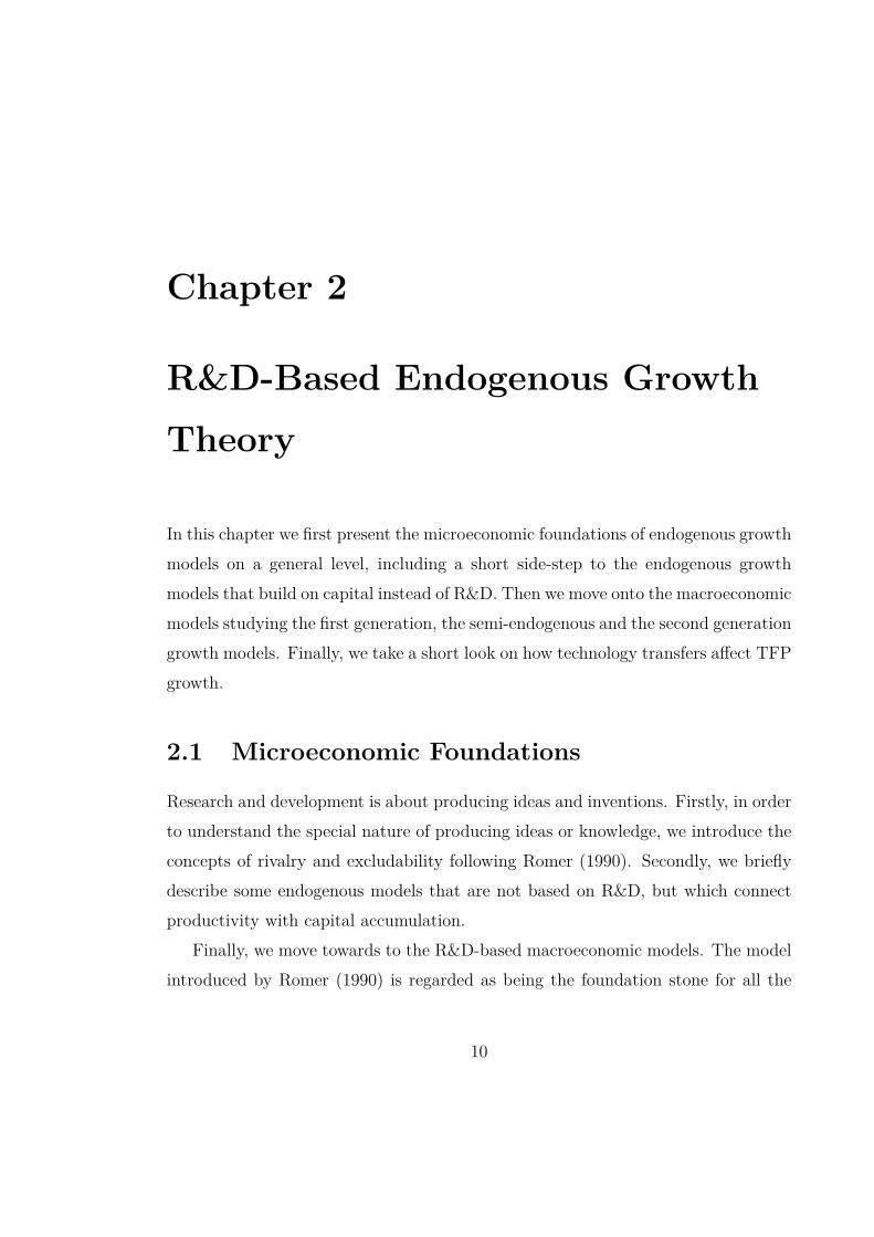
Jalava et al. (2006) have constructed the dataset so that it reflects the non-residential market sector of the Finnish economy meaning that housing services areexcluded from the data. The reason for limiting the data in such way is the fact thathousing services cannot be seen as producing anything new, but they are rather justreallocating existing assets. Therefore housing services are irrelevant for long-termgrowth. GDP is measured at basic prices. We will therefore follow this approach,and so the data on GDP and labour that has been obtained from Statistics Finlandfor the years 1975–2008 has also been treated to correspond to the non-residentialmarket sector and GDP is at basic prices.
Figure 3.1 shows the logarithmized and indexed series of GDP and hours worked.GDP seems to have been growing rather steadily, but the number of hours workedhas decreased from late 50’s. A sharp decrease was experienced during the severedepression in the early 90’s resulting in severe unemployment of which the recoveryhas been really slow.
1960 1970 1980 1990 2000 2010
0.95
1.00
1.05
GDPL
Figure 3.1: GDP and labour (indexed)
38

We calculated a total of seven measures for total factor productivity for theyears 1955–1974 as a Solow residual, from both CES and Cobb-Douglas productionfunctions with several parameter values that Jalava et al. (2006) used in their article.
First, the CES production function is defined as
(3.1) Yt = At[δK−ρt + (1− δ)L−ρt ]−1ρ .
By taking logs and rearranging we can calculate total factor productivity, denotedby A, as what is left unexplained from capital and labour
(3.2) lnAt = ln Yt + 1ρ
[ln δK−ρt + (1− δ)L−ρt
].
Jalava et al. (2006) obtained four plausible values for ρ: 0.389, 0.851 (twice) and0.854. We also used the average of them all, 0.687.22
With these four different values we constructed four TFP-series to see which onegave the most compatible result with the Statistics Finland data. Parameter δ wasfixed to 0.5 in all the cases. Since Statistic Finland uses Cobb-Douglas productionfunction in calculating their TFP index we also examined three possible variationsof the Cobb-Douglas production function
(3.3) Yt = AtKαt L
1−αt ,
from which we calculated A by taking logs and subtracting
(3.4) lnAt = ln Yt − [α lnKt + (1− α) lnLt] .22In fact they estimated parameter σ = 1/1 + ρ which gave the values 0.72, 0.57 and twice 0.54.
We also used the average of them all, 0.593.
39

We constructed three series with different values of α: 0.5, 0.4 and 0.3.So finally we had a total of seven different TFP-series. We inspected the over-
lapping period, 1975–2003, of each of the seven series and the Statistics Finlanddataset. The data used in the estimations was chosen by graphically inspectingthe datasets and by studying the stationarity of the difference of the datasets. Thevariable that gave the "best-fitting" result with the Statistics Finland data was TFPcalculated with CES production function with the choice of ρ being 0.687.
Figure 3.2 shows the level of productivity (log) and its growth rate. Total factorproductivity has been growing rather steadily since 1955.
1960 1970 1980 1990 2000 2010
0.6
0.8
1.0
1.2
1.4
1.6
1960 1970 1980 1990 2000 2010
−0.
020.
000.
020.
04
Figure 3.2: Left: TFP (log), right: TFP growth rate.
There does not appear to be a trend in the growth rate, it seems to be fluctuatingaround a positive mean value near 2 percent, thus there is resemblance in the Finnishand U.S. TFP developments.
3.2 R&D Input Variables
Data on R&D input has also been gathered from separate sources. Data on R&Dexpenditures R and workforce N as well as person-years Ny are from StatisticsFinland for the years 1971–2008. For the years 1955–1970, R&D expenditures are
40

obtained from Saarinen (2005). In the Statistics Finland data there are some in-dividual missing values that we treated with linear interpolation. Saarinen (2005)reports only 5-year averages (for years 1955–1970) expressed as percentage of GDP.We used the GDP data from Jalava et al. (2006) to calculate the real values of R&Dexpenditures and set the three five year -average values given by Saarinen (2005) tocorrespond the expenditures in 1957, 1962 and 1967 and used linear interpolationto derive the remaining values during for 1955–1970. The Statistics Finland data onR&D expenditures has been deflated with the same GDP deflator used by Jalava etal. (2006).
The patent data is from The World Intellectual Property Organization (WIPO),we denote total number of patent applications by PA and total number of patentgrants by PG. The data has been constructed using two different time series, foryears 1955–1994 we have used patent applications by patent office Finland (PRH)23
and for years 1996–2008 we have used patent applications by country of origin (1995–2008). The country of origin -series are only available since 1995. The criterionfor allocating patent applications to a particular country of origin is residency ofthe first-named applicant. Resident applications in Finland include all applicationsreceived by the PRH with a first-named applicant residing in Finland. For Fin-land, applications filed abroad include all applications filed with other patent officesaround the world with a first-named applicant residing in Finland (WIPO 2010).
The reason for WIPO to have constructed a new series is because an increas-ing amount of patent applications are sent to some international patent offices.Finland joined the European Patent Office (EPO) in 1995 and since then an in-creasing amount of Finnish patents have been filed through EPO and the numberof patents filed through the Finnish patent office PRH, has been decreasing signifi-cantly. Therefore combining these series at the date when Finland joined EPO gives
23The statistic can be broken down by resident and non-resident. Resident filing refers to anapplication filed at an Office of or acting for the State in which the first-named applicant in theapplication concerned has residence. Non-resident filing refers to an application filed at an Officeof or acting for the State in which the first-named applicant in the application concerned does nothave residence (WIPO 2011). Here we use the total count.
41

a much more realistic view on the development of the number of Finnish patents thanusing the old series. The two datasets have nearly the same value for year 1995, andthe small difference can be explained since the data of origin be incomplete (WIPO2011).24 Figure 3.3 describes how the datasets have been combined.
1960 1970 1980 1990 2000 2010
020
0040
0060
0080
0010
000
Patent applications by patent office Patent applications by country of origin
1960 1970 1980 1990 2000 20100
1000
2000
3000
4000
5000 Patent grants by patent office
Patent grants by country of origin
Figure 3.3: Combining the patent data up left: solid: Number of patent applicationsby office, dash: Number of patent applications by country of origin. Up right: solid:Number of patent grants by office, dash: Number of patent grants by country oforigin.
The benefit of the data on the number of patents is that it is easily available as along time series. However, even though it has been used very widely as an indicatorof innovative activity it is becoming less common in recent literature.25 Trajtenberg(1990) criticizes the use of patents counts since the value of patents varies largely,and therefore he proposes a citations-weighted measure of patents to correct for thisflaw. However, this would not be a problem if the average value of patents hadbeen approximately constant over time but as Caballero & Jaffe (1993) claim, eventhe citations-based measures of the average value of patents have been changingover time. Another problem is that the propensity of patenting might have alsochanged over time, for instance Griliches (1990) finds indirect evidence of the costs
24WIPO (2010) reported that it was not able to determine the country of origin for around 7percent of total patent applications filed in 2008.
25For instance Ha & Howitt (2007), and Jones (2002) have no patent data, Coe et al. (2009) usean index of the strength of patent protection.
42

of patenting having increased over time. Nevertheless, as Madsen (2008) points out,patent counts still have the advantage that informal R&D is also patented.
Data on high technology imports (denoted as I) is gathered from the CustomsInformation Service Archives statistical yearbooks for years 1955–1986 and fromUljas database for years 1987–2008. The series has been weighted with the GDPdeflator by Jalava et al. (2006). The Standard international Trade Classification(SITC) has been used in choosing the products that can be understood as hightechnology. The SITC subgroups chosen for high technology has been reported inAppendix D.
Variables used in estimations are all logarithmized. Note that the variables R,A, I, PA and PG are from years 1955–2008, whereas N and Ny are only availablefor 1971–2008.
3.3 Variables Indicating Semi-endogenous
R&D Input
The semi-endogenous growth theory suggests that having total factor productivitygrowth without a trend would indicate that there should be no trend in the growthrate of R&D input either (Ha & Howitt 2007). The growth rate of TFP has not hada statistically significant linear trend, which is also apparent from figure 3.2.26
Another result suggested by the semi-endogenous growth theory is that thereexists a cointegrating relation between TFP and R&D input. We will study thismore closely in chapter 5, but roughly put this would mean that there is a lineardependency between TFP and R&D input that prevents them from diverging toomuch from each other. The graphical implication of this would be that in an idealcase, the two series move "hand-in-hand".
26We estimated a deterministic linear trend by using OLS with heteroscedasticity and autocor-relation consistent (HAC) standard errors. Trend annual change is the OLS-estimator β from theequation gX = α+ β×Y EAR.
43

Now we will take a closer look to the R&D input variables. The variable indi-cating R&D input for the semi-endogenous model is the one that we refer to as X.As empirical counterparts we use seven variables (all logs): R&D expenditures (R),productivity adjusted R&D expenditures (R/A), high technology imports (I), num-ber of R&D workers (N), number of person-years in R&D (Ny), (in a similar manneras Ha & Howitt) patent applications (PA) and patent grants (PG) (as Madsen etal.).27
The levels of R&D input -variables are presented together with TFP in figure 3.4.Like TFP, also the R&D variables have been increasing rather linearly over the years.However, growth in TFP has been much faster than growth in any of these R&Dinput variables. Only the growth rate of R&D expenditures is almost as rapid as thegrowth rate of TFP. This result does not however hold for the productivity adjustedR&D expenditures, since the adjustment starts slowing down growth significantlyafter the 70’s. At this point it seems that there might be a cointegrating relationwith a trend present in most of the models.
Since the semi-endogenous growth theory implies that given a trendless growthrate in TFP, also the growth rate of R&D input should be trendless, we have alsoplotted the growth rates of R&D input in figure 3.5.
Growth of high technology imports has no statistically significant linear trendand neither do the growth rates of patent variables, which have been fluctuating nearzero, although it is noteworthy that both of them have significant volatility peaks.However, both R&D expenditure -variables have a statistically significant downwardtrend at the 95% level. A similar trend is apparent also in R&D workforce variables,however none of these trends are statistically significant at the 95% level. In R&Dexpenditures -variables and in the number of R&D person-years the growth has beensmoothest.
Like the U.S., also Finland has experienced trendless TFP growth. However, Ha& Howitt (2007) found that the growth rates of R&D input have been declining,
27A table of the empirical variables is presented in Appendix A.
44
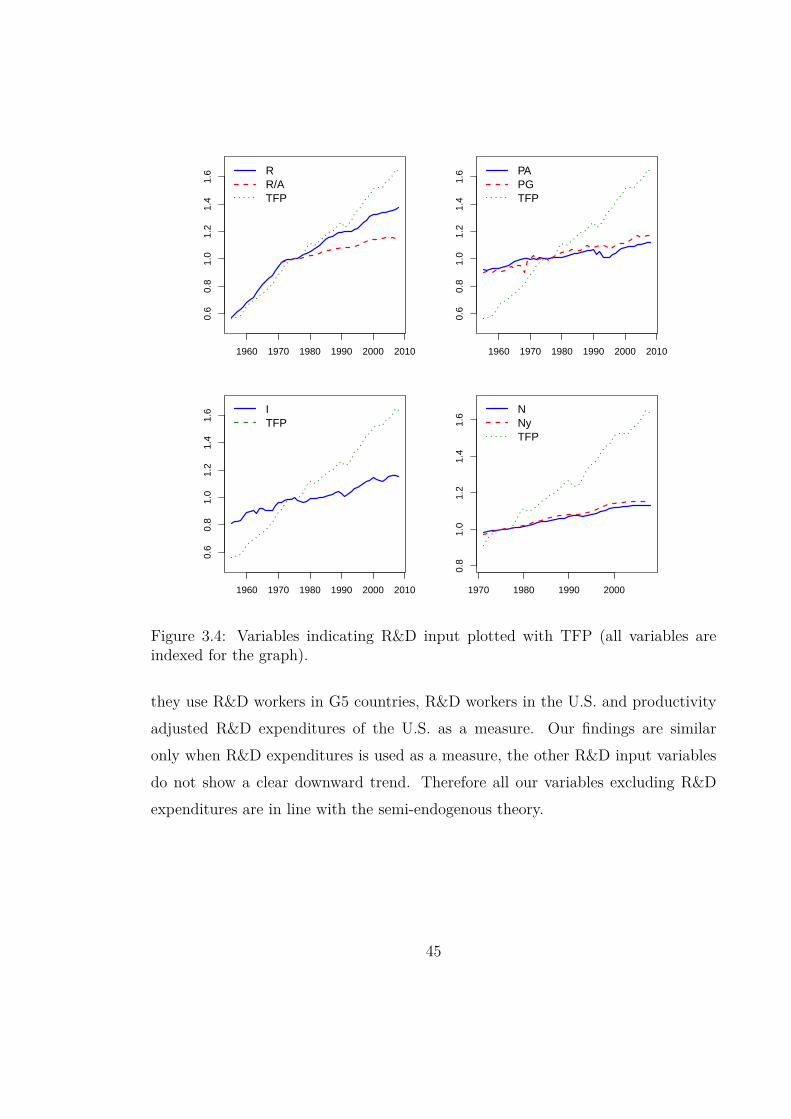
1960 1970 1980 1990 2000 2010
0.6
0.8
1.0
1.2
1.4
1.6 R
R/ATFP
1960 1970 1980 1990 2000 2010
0.6
0.8
1.0
1.2
1.4
1.6 PA
PGTFP
1960 1970 1980 1990 2000 2010
0.6
0.8
1.0
1.2
1.4
1.6 I
TFP
1970 1980 1990 2000
0.8
1.0
1.2
1.4
1.6
NNyTFP
Figure 3.4: Variables indicating R&D input plotted with TFP (all variables areindexed for the graph).
they use R&D workers in G5 countries, R&D workers in the U.S. and productivityadjusted R&D expenditures of the U.S. as a measure. Our findings are similaronly when R&D expenditures is used as a measure, the other R&D input variablesdo not show a clear downward trend. Therefore all our variables excluding R&Dexpenditures are in line with the semi-endogenous theory.
45

1960 1970 1980 1990 2000 2010
−0.
10.
00.
10.
20.
3
R R/A
1960 1970 1980 1990 2000 2010
−0.
4−
0.2
0.0
0.2
0.4
0.6
PAPG
1960 1970 1980 1990 2000 2010
−0.
2−
0.1
0.0
0.1
0.2
0.3 I
1970 1980 1990 2000 2010
−0.
050.
000.
050.
10
NNy
Figure 3.5: Variables indicating growth of R&D input.
3.4 Variables Indicating Schumpeterian R&D In-
tensity
If the data was generated by a Schumpeterian growth model, the constancy inproductivity growth implies that there should be no trend in R&D intensity, whichis defined as R&D input X adjusted with the product proliferation variable Q. Ha& Howitt (2007) use three different measures for Q: Y , L and hL, where h is humancapital. We here use the first two measures (due to us not having data on humancapital). Thus we have a total of fourteen variables indicating R&D intensity.
46
The assumption of having no trend in R&D intensity is backed up by the U.S.and G5 evidence presented in Ha & Howitt (2007). The theory also suggests thatthere is a firm cointegration relation between R&D input and product variety, sothat they go "hand-in-hand" and their log-difference (lnXt − lnQt) is a stationaryprocess.
R&D intensity -variables (or to be precise the log-differences) are presented infigure 3.6. The Finnish evidence seems to be quite different from the U.S. Whenadjusted with labour L the increasing trend is visible in all of the variables, sinceas we already saw, labour as measured by hours worked, has not been growing inFinland. The increasing linear trends in all the intensity -variables using L, arestatistically significant at a 99% level.
However, adjusting R&D input with GDP partially offsets the trend in the R&Dinput. The slope of the trend has indeed decreased in most of the cases but noneof the variables still seem to be fluctuating around a constant, except maybe thepatent variables. The trend tests suggests that the only variable with no statisticallysignificant trend is patent applications adjusted with GDP.28
The semi-endogenous theory also suggests that R&D intensity variables shouldbe stationary. Just by looking at the figures it also seems like none of the variablesadjusted with labour are stationary and from those adjusted with GDP it lookslike at least R&D expenditure and workforce intensity -variables are not stationary.This inspection is in line with our empirical findings presented in chapter 5, the onlymodel where the data fits the model that incorporates this assumption is patentapplications adjusted with GDP.
Labour (as measured by hours worked) thus seems to be a very poor measure ofthe "scale" or the "product variety" of the in the Finnish case, since even though therehas been significant economic growth, it is not due to the increase in labour input.Nonetheless, our other measure of product proliferation, GDP, has had a clearlyincreasing trend and probably is as good a proxy for the scale of the economy for
28Note that the y-axis of each graphs plotted next to each other are of the same length.
47

Finland as it is for the U.S. As we show in the estimation results in chapter 5, theSchumpeterian model fits the data just slightly better when GDP is used as productvariety instead of labour (even though in that case also, very poorly). Theoreticallyhowever, there is no reason to oppose the use of labour as product variety measure.
48

1960 1980 2000
−6
−5
−4
−3
−2
−1
01
R/LR/AL
1960 1980 2000
−7
−6
−5
−4
−3
−2
−1
0
R/YR/AY
1960 1980 2000
−2.
0−
1.0
0.0
0.5
1.0
PA/LPG/L
1960 1980 2000
−4.
0−
3.0
−2.
0−
1.0
PA/YPG/Y
1960 1980 2000
−2.
0−
1.0
0.0
1.0 I/L
1960 1980 2000
−3.
5−
2.5
−1.
5−
0.5 I/Y
1970 1980 1990 2000 2010
0.5
1.0
1.5
2.0
2.5
3.0
N/LNy/L
1970 1980 1990 2000 2010
−1.
5−
0.5
0.0
0.5
1.0
N/YNy/Y
Figure 3.6: Variables indicating R&D intensity X/Q.
49

Chapter 4
Econometric Methods: VectorAutoregressive and Vector ErrorCorrection Models
In this chapter we present the econometric methods used in studying the relationbetween R&D input and total factor productivity by using a cointegrated vectorautoregressive model.
The model in interest is a VAR-model for variables that are (asymptotically)nonstationary and have a unit root e.g. are integrated of order one (denoted here-after as I(1)). A VAR-model for I(1)-variables is presented in a so-called vector errorcorrection (VECM) -form. Integration of order one means that when we differen-tiate the time series it will be a stationary process (denoted by I(0)). Graphicalinspection of our variables allows us to assume that these variables are generated bya nonstationary process and the formal proof will be presented in chapter 5.
We estimate the general form of the productivity-growth function of R&D-basedendogenous growth models by Ha & Howitt (2007), which we call the unrestrictedmodel, with the Johansen maximum likelihood approach (see for example Johansen1995, 1988; Johansen & Juselius 1990 and Johansen 1991) and the semi-endogenous
50

and the Schumpeterian models (the restricted models) with a simple two stepmethod (S2S) (see for example Ahn & Reinsel 1990, or Lütkepohl & Krätsig 2004,ch. 3).
The VAR-model which is a multivariate time series model with p variables is ofthe form (Johansen 1995)
(4.1) Xt = Π1Xt−1 + ...+ ΠkXt−k + ΦDt + εt, t = 1, ..., T
where Xt is a p-dimensional autoregressive process (with now all its variables be-ing I(1)) and Dt consists of deterministic variables such as a constant and trend (andcan also have any non-stochastic variable such as seasonal dummies). Π1, . . . ,Πk
and Φ are coefficient matrices and εt ∼ iid(0,Ω) is an error term.A VAR-model is used in this form when one wants to study the relations be-
tween stationary time series. However, even though the representation can be usedfor nonstationary series, we will have to modify the VAR-model in order to studythe relations between nonstationary time series. For these nonstationary series thegeneral VAR-model can be represented in a Vector Error Correction Model (VECM)form29
(4.3) ∆Xt = ΠXt−1 +k−1∑i=1
Γi∆Xt−i + ΦDt + εt,
29Starting from the VAR form in equation 4.1 we get the VECM-form by defining a polynomialmatrix Π(B) = In − Π1B − . . . − ΠkB
k (using a property of a lag-operator Π(B) = Π(1) + (1 −B)G(B), where R(B) =
∑∞j=0 CjB
j , and∑∞j=1 ‖ Cj ‖ < ∞, without going further to its details)
we can write the polynomial as
(4.2) Π(B) = Π(1)B +(In −
k−1∑i=1
ΓiBi)
∆,
so using this in equation 4.1 gives us
51

where thus Π = ∑ki=1 Πi − In. The deterministic terms ΦDt enable the rela-
tionship between the variables to change over time. As we see, the LHS is now adifference of Xt and therefore stationary. Also the lags are differences apart fromthe term ΠXt−1, which is called the error correction term. However, since all otherterms in the equation clearly are stationary, this term also needs to be stationary.By estimating matrix Π we can find out whether there are linear combinations ofthe variables in Xt−1 that are stationary. If linear combinations of the nonstationaryvariables exist, the linear combinations are then stationary, I(0), and the variablesincluded in the linear combination are said to be cointegrated.
Therefore the test for cointegration between variables in Xt−1 is done by esti-mating the coefficient matrix Π. If there is no cointegration between the variables,then Π has full rank, p. If cointegration exists the rank is r (r < p). The hypothesisthat Π has rank r can be expressed as
(4.4) H(r) : Π = αβ′
where α and β are p×r matrices. Matrix β defines the cointegrating vectors andelements in α are known as adjustment parameters. By replacing Π in equation 4.3with αβ ′ , we have the reduced form error correction model. (Johansen 1995, ch. 5)presented here again for clarity
Π(B)Xt =(
Π(1)B +(In −
k−1∑i=1
ΓiBi)
∆)Xt
= Π(1)Xt−1 + ∆Xt −k−1∑i=1
Γi∆Xt−i
= ΦDt + εt
where Γi = −∑kj=i+1 Πj . By replacing Π(1) = Π we get equation 4.3.
52

(4.5) ∆Xt = αβ′Xt−1 +
k−1∑i=1
Γi∆Xt−i + ΦDt + εt.
When the hypothesis of r cointegrating vectors holds, β ′Xt is stationary.
In determining the cointegration rank we use a likelihood ratio tests, the tracetest. The model that we estimate for the trace test is a VAR with a constant (andno trend). In this case the deterministic term in equation 4.3 is defined as Dt = µ0.The constant term can be thought to be inside the cointegration relation so thatmodel 4.3 can be written as
(4.6) ∆Xt = Π∗ Xt−1
1
+k−1∑i=1
Γi∆Xt−i + εt,
where Π∗ = [Π : ν0] is K × (K + 1) with ν0 = −Πµ0. This model is used fortesting the statistical significance of Π with the reduced rank -hypothesis (Johansen1995, ch. 6). The test is defined as
(4.7) − 2 lnQ(H(r)|H(p)) = −Tp∑
i=r+1ln(1− λi),
where eigenvalues λi are the squared canonical correlations. The trace statisticthus tests the null hypothesis of r cointegrating vectors against the alternative hy-pothesis of p cointegrating vectors (Johansen 1995, ch. 6). The test statistic doesnot follow a commonly known distribution; the asymptotic distribution is definedas
53

(4.8) 2 lnQ(H(r)|H(p))→ tr
1∫
0
(dB)F ′ 1∫
0
FF ′du
−1 1∫0
F (dB)′
where F = B is a p − r dimensional Brownian motion. The critical values areobtained by simulation (Johansen 1995, ch. 15).
After the cointegrating rank has been determined, the matrix Π = αβ′ and also
the Γi matrices can be estimated. It is noteworthy that since we estimate first therank of the matrix, we have as a result a certain number of vectors that span thecointegrating space. There is thus no unique solution to Π, but there are manypossible α and β that contain the cointegrating relations or linear transformationsof them.30 Thus no economic interpretation can be given to α and β.
A unique (identifying) and consistent solution can be obtained by imposing in-dentifying restrictions. A common restriction is to set β ′ = [Ir : β ′
K−r], where β′K−r
is a (K − r) × r matrix. For r = 1 (which is the case we are considering later inchapter 5), the normalization reduces to a case where one element of the β-vectoris set to one.
This kind of normalization is not however a trivial task, economically inter-pretable cointegrating results should emerge from the estimation and an unsuitablenormalization may cause problems (for example if we normalize by a variable thatdoes not belong to the cointegrating relation). We will not however go deeper intothis question, since in our model, the normalization vector is given by theory.
An important outcome of normalized vectors is that we are able to find if there arevariables that are in fact stationary processes. For the normalization case described,if any of the r variables with respect to which we normalize were a stationary process(thus the ones corresponding to Ir), the estimates of the vector, β ′
K−r would be zero(Lütkepohl 2005, ch. 6).
After having determined the cointegration rank, the Johansen maximum likeli-30Since Π = αβ
′ = (αξ−1)(βξ′)′ with a non-singular r × r matrix ξ.
54

hood procedure is used to estimate α, β and Γi. The ML-estimator of β definesthe combination of Xt−1 that yields the r largest so-called canonical correlations of∆Xt with Xt−1 (after correcting for lagged differences and deterministic variables).Intuitively, β -matrix describes the long run relations of the variables in question,which is what we are interested in.
Matrix α is often called "loading matrix" or "adjustment matrix" meaning thatfor each equation of the model, it gives the weights attached to the cointegratingrelations. These estimates represent how the deviations from the long-run relationsaffect the changes in the variables observed. Matrix α can be used to study if any ofthe variables in the study is weakly exogenous. In the case where the cointegratingrank is one, thus both β and α are vectors, having the ith element of α equal to zero,would mean that the ith variable is weakly exogenous. Thus an intuitive explanationfor the weak exogeneity is that the variable can be regarded as representing a sort of"explanatory variable", even though this term is not used in the literature. The Γimatrices are connected to the short run dynamics of the model, but their analysisis left out from this study.
The distributions of β, α and Γi are Gaussian when we condition on the ob-servations of explanatory variables. The unconditioned distribution is however notnormal, but it is a so-called mixture of Gaussian distributions. In statistical infer-ence only the conditional distribution is needed so we do not explain the propertiesof the mixture of Gaussian distributions here. We can thus conclude that we use anasymptotic normal distribution to determine the critical values of the parameters ofβ (as well as α and Γi) and an asymptotic χ2 -distribution in the Wald test (see forexample Johansen 1988, 1991).
The unrestricted model is estimated with the Johansen approach but the semi-endogenous and Schumpeterian models are estimated with the so called simple twostep (S2S) method (see Ahn & Reinsel 1990; Lütkepohl & Krätsig 2004).
Estimation of the semi-endogenous and Schumpeterian model is done so thatthe cointegration rank is set to one in all of the cases and then restrictions to the
55

parameter vector β are imposed.After we have used the Johansen procedure in estimating the unrestricted model,
we can in that framework test restrictions of the form
(4.9) H0 = Rvec(β∗′
K−r) = r vs. H1 = Rvec(β∗′
K−r) 6= r,
When J is the number of linearly independent restrictions for the coefficients ofβ∗
′K−r, then R is a J × (K − r)r coefficient matrix and r is a J -dimensional vector.
A Wald test is used with a χ2(J) distribution (Lütkepohl & Krätsig 2004, ch. 3).After running the Wald test we can estimate the restricted models with the
simple two step (S2S) method. For complex restrictions the Johansen approach iscomputationally more demanding, and the S2S gives a solution in closed form. TheJohansen approach is thus feasible for the models we are estimating but the softwarethat we use, JMulti, has restricted the estimation of models where restrictions on βare imposed to S2S only.
The simple two step estimation represents equation 4.3 as
(4.10) ∆Xt − Π1X(1)t−1 −
k−1∑i=1
Γi∆Xt−i = Π2X(2)t−1 + ut,
where X(1)t−1 is r×1 and X(2)
t−1 is K−r×1. The matrices Π1 and Π2 are K×r andK ×K − r, respectively such that [Π1 : Π2] = Π1 = αβ
′ . With the normalizationΠ1 = α and Π2 = αβ
′K−r.
Only the general idea of the S2S estimation is presented here. In the two-stepprocedure the first step eliminates the short-term parameters by replacing themwith their OLS estimators. Then it is possible to estimate Π = [Π1 : Π2] with OLSand obtain the estimator for α. With these results, it is possible to estimate theresulting free parameters β ′
K−r with OLS.
56

In the S2S estimation a formulation for the restrictions in β is defined as β =Hϕ.31 In the restricted case we first get an estimator for ϕ from where we getthe final restricted estimator β = Hϕ (Lütkepohl & Krätsig 2004, ch. 3). The S2Sestimator has same asymptotic properties as the ML estimator obtained in Johansenapproach (Ahn & Reinsel 1990). Thus for inference we can therefore use normaldistribution. Also other parameters of the model, Γi and deterministic terms, canbe estimated with S2S.
31Details of this restriction are intentionally left out.
57

Chapter 5
Results
In this chapter we report and discuss our results from estimating the productivity-growth function introduced by Ha & Howitt (2007) with the Finnish data.
The general result from the estimation is that there is clear evidence to supportthe semi-endogenous model but the Schumpeterian model does not fit the Finnishdata, however we cannot fully reject the Schumpeterian idea of product prolifera-tion. Our estimation technique can be argued to be relatively robust compared tothose used by Ha & Howitt (2007) and Madsen et al. (2010). They use two separatestatistical frameworks in estimating the model whereas our submodels are statisti-cally defined as "nested models"; they use a common framework in which parameterrestrictions are imposed.
5.1 Estimation Equation
The estimated equation is the general form of the growth models, equation 2.1:
gA = λ
(X
Q
)σAφ−1,
where in steady state
58

Q ∝ Lβ.
By taking logs and making a discrete time approximation of the equation insteady state we obtain32
(5.1) ∆ lnAt = γ0 + γ1
(lnXt − β lnQt + φ− 1
σlnAt
)+ εt,
where εt is an error term, which is identically and independently distributed withmean zero. A cointegration relation would mean that when ∆ lnAt is stationary,then the term inside the brackets
(5.2) Et = lnXt − β lnQt + φ− 1σ
lnAt,
denoted now by Et, would also be stationary. Then for the semi-endogenoustheory where β is zero and thus lnQt vanishes, equation 5.2 reduces to the form
(5.3) Eset = lnXt +
(φ− 1σ
)lnAt,
where the superscript in Eset stands for semi-endogenous. Note that coefficient
φ−1σ< 0, since the theory states that φ < 1 and σ > 0.According to the semi-endogenous theory, having Ese
t as a stationary processwould mean two things: that the linear combination of lnX and lnA must be sta-tionary, hence if the two variables are nonstationary, then they must be cointegrated.
In the Schumpeterian model equation 5.2 reduces to the form
32since ∆ lnAt = lnλ + σ(
lnXt − β lnL− φ−1σ lnAt
), now γ0 denotes lnλ and γ1 denotes the
σ outside the brackets.
59

(5.4) Esct = lnXt − lnQt,
where the superscript in Esct stands for Schumpeterian. Since the theory claims
that φ = 1, the term(φ−1σ
)lnAt vanishes from the equation.
Unlike Ha & Howitt (2007) and Madsen et al. (2010) we will estimate the gen-eral form presented in equation 5.2 first, so that no parameter restrictions of thesubmodels are taken into consideration. This model is not backed up any economictheory as such. On the contrary, it is more like a compromise between the modelsand therefore intriguing to estimate.33 If the freely estimated parameters did notfit the model, roughly it would indicate a rejection of the R&D-based models in alarger sense implying that R&D-based endogenous growth theories do not describewell the Finnish productivity growth. However, as described in more detail later,the unrestricted models are generally well specified and do support the idea thatFinnish productivity growth is driven by some kind of R&D-based growth model ingeneral.
If, hypothetically, this general form of the model gave a good description of thedata the three variables should be cointegrated as presented in equation 5.1, so thatβ = 0 or β = −1 and φ−1
σ≤ 0. In estimating the general model it makes sense
to estimate β freely so we expect it to be between 0 and -1. If we allowed for theparametrization considered by Jones (1999), β could also be smaller than -1.
The hypothesis that the data was generated by a semi-endogenous growth modelwould imply one restriction to the unrestricted model, namely H0: β = 0, so thatthere exists a cointegrating relation between R&D input and TFP. The restrictionφ−1σ≤ 0 is also assumed as previously, but not formally imposed.The hypothesis that the data was generated by a Schumpeterian growth model
instead would indicate a joint hypothesis of two restrictions, H0: β = −1 and33Compromising between the models is also attempted by Jones (1999) who studies a model
with unrestricted β and φ < 1, thus not far from the restrictions in our general model.
60

φ−1σ
= 0 (since φ = 1).34
This estimation can be argued to be very robust compared to the estimations ofboth Ha & Howitt (2007) and Madsen et al. (2010). Ha & Howitt (2007) estimatethe semi-endogenous model with cointegration but leaving the product proliferationvariable outside the estimation, therefore there is no restriction to study the validityof the hypothesis β = 0 as in our study. The estimation of the Schumpeterian modelreduces to a unit root test and as a matter of fact Ha & Howitt (2007) have studiedthe model only by running an ADF-test to the difference of Xt and Qt. Hence,they do not get any support for their claim that φ−1
σ= 0. Madsen et al. (2010)
have used cointegration in estimating the Schumpeterian model, but unlike us, theyhave estimated freely the coefficient of Q so that the equation is as a matter of factEsct = lnXt − β lnQt.However, by estimating the nested model, we are able to make inference on all
of the parameter restrictions suggested by both of the models and compare them ina robust way. Finding firm support for the semi-endogenous model and almost nosupport for the semi-endogenous model in this statistically comparable frameworkcan be regarded as very firm evidence for the Finnish case compared to the contra-dictory evidence presented by Ha & Howitt (2007) of the U.S. and Madsen et al.(2010) of India.
5.2 Cointegration Test of the Unrestricted
Model
The results of the unrestricted model are presented in table 5.1. The first columnstell the result of the trace test and for clarity the number of cointegration vectorsgiven by the test is presented in column r(95%, 99%). However, since our theorystates that there exists only one cointegration vector, we have restricted the rank ofβ to one in all the cases in the table. The estimated cointegrating vector is presented
34Thus in all of these cases we have normalized the cointegration vector to the term lnXt.
61

in the last column, standard errors are in brackets. All of the cointegrating residualsare presented in figures 5.1, 5.2 and 5.3.
The lag length of the model was chosen so that in the VAR-form of the modelsthere is no autocorrelation of residuals. In all of the models include an intercept anda trend. The residual diagnostics of the VAR are reported in the Appendix, tableC.1. The trace test for determining the cointegration rank was then conducted tothis VAR-model and the resulting VECM-model is unrestricted in the theoreticalsense but restricted in as having one cointegrating vector. All of the VECM-modelsincluded an intercept outside the cointegration relation but no trend. Residualsdiagnostics of the unrestricted model are reported in table C.2.
Estimation of the general form model reveals that R&D-based growth theoriesare generally speaking capable of explaining Finnish productivity growth. The sub-stantial differences in the product proliferation and R&D input measures used ishowever visible in the results. Despite the differences, almost all the models are wellspecified (autocorrelation is present in only three cases) and there can be said to besome sort of cointegration (rank being either one or two) in 11/14 cases and preciselyone cointegrating vector in 8/14 cases (when both reported confidence intervals areconsidered). Almost all of the parameter estimates are statistically significant (atthe 95% level as much as 22/28 and at the 99% level 18/28 of all the parameterestimates).
Since the estimates are different from zero we can also draw the conclusion thatthe assumption of a unit root process holds as explained in chapter 4. However,since the cointegration vector is normalized to the R&D input variables, the unitroot of three variables, A, Y and L, is not being studied. Therefore we ran an ADFtests to these three variables and in all the cases we could not reject the null of theunit root even at the 90% confidence level, the results are reported in Appendix B.Thus the assumption of all the variables being created by a nonstationary processholds.
The results favouring the semi-endogenous model and refuting the Schumpete-
62

R & L
1960 1970 1980 1990 2000 2010
−61
0−
600
R & Y
1960 1970 1980 1990 2000 2010
−31
.1−
30.8
RA & L
1960 1970 1980 1990 2000 2010
−61
0−
600
RA & Y
1960 1970 1980 1990 2000 2010
−31
.1−
30.8
I & L
1960 1970 1980 1990 2000 2010
19.3
19.6
19.9
I & Y
1960 1970 1980 1990 2000 2010
11.9
12.1
12.3
Figure 5.1: The cointegrating residuals of the unrestricted models with R&D ex-penditures, productivity adjusted R&D expenditures and high technology imports.
rian are not as clearly visible in the general model as it is in the nested models.However, we can clearly see that even though the product proliferation variables arestatistically significant, only 6 of the 14 estimates have a confidence interval thatincludes the value -1 and also 6 of the parameter estimates of φ−1
σhave zero inside
the confidence interval, results that would favour the Schumpeterian model. Themodels with GDP indicating product variety look just slightly more promising forthe Schumpeterian model.
On the contrary for the semi-endogenous case, 11 of the 14 estimates for φ−1σ
arenegative, thus of the right sign. However, none of the product proliferation variableshas the value zero inside the confidence interval, thus we cannot reject the hypothesisthat product variety plays a role in the kind of R&D based endogenous growth that
63

PA & L
1960 1980 2000−
18.0
−17
.7
PA & Y
1960 1980 2000
−7.
4−
7.0
PG & L
1960 1980 2000
−7.
2−
6.8
PG & Y
1960 1980 2000−
5.3
−5.
0−
4.7
Figure 5.2: The cointegrating residuals of the unrestricted models with patent ap-plications and patent grants.
Finland has experienced. But as the estimation of the Schumpeterian model reveals,product variety cannot be said being strictly proportional to the R&D input in away suggested by the Schumpeterian model.
We will not study more closely the 14 different models estimated because it ismore interesting to study them inside the nested models. However, we will presentbriefly some interesting remarks. Two of the three models with high autocorrelationswere models with an R&D workforce variable and the models with these variableswere also the ones that had no cointegration. It is a peculiar result since R&Dworkers are regarded as being a rather good proxy for R&D activity. However, wemust keep in mind the shorter time span of these variables. Therefore it is plausiblethat the results differ from others so much because the sample size is not largeenough for asymptotically as valid estimation results as the other models have.
It is also noteworthy that three of the models have estimates that are very large
64

N & L
1975 1985 1995 2005−
3.4
−3.
1−
2.8
N & Y
1975 1985 1995 2005
−0.
80−
0.65
−0.
50
Ny & L
1975 1985 1995 2005
−40
2−
396
−39
0
Ny & Y
1975 1985 1995 2005−
0.80
−0.
65−
0.50
Figure 5.3: The cointegrating residuals of the unrestricted models with R&D work-force and R&D person-years.
in absolute value. This result is no more present in the estimations of the nestedmodels, so it could be a difference arising from the two different estimation methodsused, the Johansen approach and the S2S approach but we cannot be sure aboutthis.
5.3 Cointegration Test of the Semi-Endogenous
Model
The semi-endogenous model is formed by restricting the general model so that β = 0.This restriction is tested with the Wald test (with the alternative hypothesis beingβ 6= 0). The results of the Wald test and the estimation of the models are given intable 5.3.
The results of the Wald test indicate that the null hypothesis that the second
65

element is zero is rejected in all but three of the cases. However, the parameterestimates of the semi-endogenous model are all statistically significant at the 99%significance level and of the right sign. Most of the models also have well-behavingresiduals, but there are some exceptions where problems arise. In import and patentmodels the cointegrating residuals are clearly stationary, in R&D expenditure andworkforce models stationarity is not so evident. For each R&D input variable thecointegrating residual looks very much the same regardless of which of the twoproduct proliferation variables is used in the model (which is probably due to havingthe zero-restriction). This general inspection gives support for the semi-endogenousmodel.
Interesting additional results arising from the estimation of the semi-endogenousmodel specifically are the α-vectors. A desirable result would be that R&D inputis a weakly exogenous variable (thus the corresponding element of the α-vectornot being statistically significantly different from zero) and TFP is an endogenousvariable (the corresponding element of α being different from zero). This wouldsuggest that the adjustment from the long-run relations happens through TFP andso R&D input could be regarded as an "explanatory variable"35. Probably due tothe great differences in the variables studied, the evidence is rather mixed. In fourcases, all with R&D expenditure or workforce variables, the α connected to TFP canbe regarded as endogenous and R&D input variable as exogenous at the 95% level.In five cases, patent and import models, the relation goes the other way around,TFP is weakly exogenous and R&D input endogenous. In the rest of the cases theevidence was not clear in one way or another. Note however, that the estimatedmodel does not technically impose any assumptions on the α-vector.
Let’s study the results more closely. The model with high technology importsand output has the best result in the Wald test being the only one where the nullhypothesis cannot be rejected at the 95% level. However, the model has very highautocorrelations and the normality assumption is not met either, thus it is clearly
35Note that this is not a formal description but rather just clarifying the idea behind.
66

not a valid model. In the model with high technology imports and labour the Waldtest cannot be rejected at the 99% level. The estimates of the β-vectors in thesemodels are significant and the cointegrating residuals look stationary. The modelwith labour has well-behaving residuals and thus seems to give good support for thesemi-endogenous theory. In both of these models TFP can be considered as weaklyexogenous and high technology imports as endogenous. So the relation would mostprobably be from TFP to high technology imports and not the other way around.
I & L
1960 1970 1980 1990 2000 2010
5.5
5.6
5.7
5.8
5.9
PA & Y
1960 1970 1980 1990 2000 2010
6.4
6.5
6.6
6.7
6.8
6.9
7.0
PG & L
1960 1970 1980 1990 2000 2010
5.0
5.2
5.4
5.6
Figure 5.4: Cointegration residuals of the semi-endogenous model, up left: Hightechnology imports & labour, up right: Patent applications & output, down: Patentgrants & labour.
Also in the model with patent applications and output, the Wald test is notrejected at the 99% level and the cointegrating residual looks rather stationary, butthe residuals of the model do not meet the normality assumption. Heteroscedastityis a problem in the model with patent applications and labour.
67
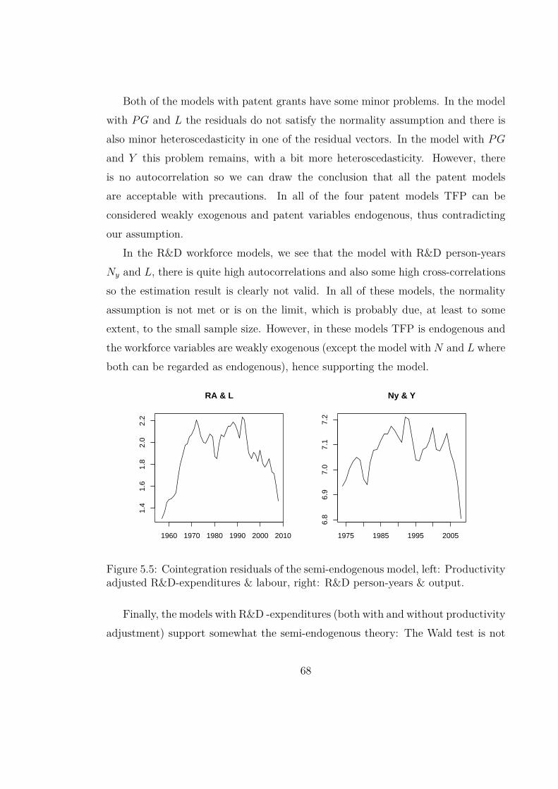
Both of the models with patent grants have some minor problems. In the modelwith PG and L the residuals do not satisfy the normality assumption and there isalso minor heteroscedasticity in one of the residual vectors. In the model with PGand Y this problem remains, with a bit more heteroscedasticity. However, thereis no autocorrelation so we can draw the conclusion that all the patent modelsare acceptable with precautions. In all of the four patent models TFP can beconsidered weakly exogenous and patent variables endogenous, thus contradictingour assumption.
In the R&D workforce models, we see that the model with R&D person-yearsNy and L, there is quite high autocorrelations and also some high cross-correlationsso the estimation result is clearly not valid. In all of these models, the normalityassumption is not met or is on the limit, which is probably due, at least to someextent, to the small sample size. However, in these models TFP is endogenous andthe workforce variables are weakly exogenous (except the model with N and L whereboth can be regarded as endogenous), hence supporting the model.
RA & L
1960 1970 1980 1990 2000 2010
1.4
1.6
1.8
2.0
2.2
Ny & Y
1975 1985 1995 2005
6.8
6.9
7.0
7.1
7.2
Figure 5.5: Cointegration residuals of the semi-endogenous model, left: Productivityadjusted R&D-expenditures & labour, right: R&D person-years & output.
Finally, the models with R&D -expenditures (both with and without productivityadjustment) support somewhat the semi-endogenous theory: The Wald test is not
68

favourable but the residual analysis suggests that the models are well defined and theparameter estimates are statistically significant. The cointegration residuals are notclearly stationary though, there seems to be first an upward and then a downwardtrend, however, there is no clear trend across the whole series. In the model withR&D -expenditures and GDP, R&D -expenditures is weakly exogenous and GDPendogenous thus supporting the model. In the three remaining cases there was noclear evidence for or against the model in this sense.
We can thus draw the conclusion that the semi-endogenous models describes wellthe Finnish economy. Most of the models are well defined and we can also say thatthe models which do not have autocorrelation but do have some heteroscedasticity ornormality -problems still, as a whole, give support for the semi-endogenous model.It also seems clear from these estimations that R&D expenditures and workforcevariables are good measures for R&D input in the sense that they were the onesthat could be regarded as weakly exogenous variables in the model.
5.4 Cointegration Test of the Schumpeterian Model
In the Schumpeterian model there are two parameter restrictions, β = −1 andφ−1σ
= 0. We ran a joint Wald test with the null hypothesis that both of therestrictions hold, against the hypothesis that neither of them holds. The results ofthe Schumpeterian estimation are reported in table 5.4. Note that unlike in the semi-endogenous model reported in table 5.3, now we have not reported the cointegrationvectors since they are the same in all of the cases. Since the model is fully restrictedand reduced to a unit root test, the estimators do not have standard errors or t-values either, analysing the model is done simply by the Wald test, the cointegratingresiduals and by residuals diagnostics. We have not analysed the α-vector in theSchumpeterian model since the model simply claims that the vertical R&D inputand horizontal product variety move "hand-in-hand", thus the weak exogeneity isnot something that would be interesting for the model. Moreover, since most of the
69

models are not well defined, the estimates for α are not even reliable.
PA & Y
1960 1970 1980 1990 2000 2010
−3.
0−
2.9
−2.
8−
2.7
−2.
6−
2.5
−2.
4−
2.3
Figure 5.6: The cointegrating residual of the model with patent applications andoutput.
There is very little evidence in favour of the Schumpeterian model. Firstly, wecan see that the results for the Wald tests are all poor for the Schumpeterian model.In all cases except one, the joint test that β = −1 and φ−1
σ= 0, is rejected both
at the 95% and the 99% level. The model with patent applications and output isthe only one that supports the restriction. The cointegrating residual of this modeldoes not have a clear trend and looks rather stationary but does have two peaksthat look striking. The latter one is probably a result of the decrease in the patentapplication series in mid-90’s (due to moving to the EU) but the previous peak, theupward peak in mid-60’s, is not so straightforward to interpret, it is probably alsodue to the patent series having a small peak around that time.
The rest of the models are all rejected in the Wald test but we can also see fromthe residual analysis that all of them have highly autocorrelated residuals. In allof the models we can reject the null that there is no autocorrelation at one lag atthe 99% level. Normality and heteroscedasticity -assumptions do hold for some ofthe models but the autocorrelations being a stronger prerequisite for a well-defined
70

model leaves us with all except one of the models being not valid. We can alsosee this from the cointegrating residuals which all look more or less nonstationary,except the model with PG and output and the model with PA and labour in whichthe cointegrating residuals look somewhat stationary, but since the models are notwell-specified, these findings are worthless.
5.5 Discussion
In this chapter, we discuss the results and compare then with first international andthen Finnish literature. Lastly we discuss the steady state properties on the modeland sum up our analysis.
5.5.1 Comparison with International Literature
In the Finnish case, the semi-endogenous model fits the data rather well whereasthe Schumpeterian model can be clearly rejected in all cases except one. However,it seems that the idea of product proliferation cannot be rejected as such.
Ha & Howitt (2007) and Madsen et al. (2010) have also compared these modelsand both of them claim that their results are clearly in favour of the Schumpeterianmodel. Like noted before however, their models are not based on the nested modelapproach like ours. Instead, in both articles the semi-endogenous theory is testedwith the Johansen cointegration test using equation 5.3, thus excluding productproliferation totally from the estimation. In Ha & Howitt (2007) the Schumpeterianmodel is estimated by testing the unit root in equation 5.4. Madsen et al. (2010)claim that in testing the Schumpeterian model they are estimating equation 5.4, butin fact, as table 1 in the article shows, they have estimated freely the coefficient ofQ, so that the equation is in fact Esc
t = lnXt − β lnQt, which is strictly speaking,not a possibility inside the Schumpeterian model (Ha & Howitt 2007).
In estimating the semi-endogenous model, Ha & Howitt (2007) find no cointe-gration between the variables. Madsen et al. (2010) also claim that they do not find
71

support for the semi-endogenous model in the Indian case, but in fact table 1 revealsthat there is cointegration in 6 out of 8 cases, of which only 2 estimates though,are of the right sign. Hence, to our view the evidence against the semi-endogenousmodel is not that unambiguous.
In support of the Schumpeterian model Ha & Howitt (2007) find clear evidencesince the null of unit root (described in equation 5.4) is rejected in all cases. Theresult of Madsen et al. (2010) of the Schumpeterian case is that in 10 out of 12cases there is cointegration, but in fact, inspection of table 2 reveals that in only 2cases the value β = −1 is inside the 95% confidence interval. Therefore Madsen’sevidence in support of the Schumpeterian model is rather weak.
Ha & Howitt (2007) also forecast TFP out of sample using both of these theo-ries. Their results suggest that the semi-endogenous theory gives a too pessimisticforecast, and that the Schumpeterian forecast fits the data better. However, in ob-taining this result, Ha & Howitt (2007) have made an additional restriction to thesemi-endogenous model and fixed the value of the parameter estimate of σ
1−φ to beequal to a value estimated in Jones (2002), so that there is a similar amount of pa-rameters to estimate in both of the models. We regard this somewhat manipulativesince the assumptions of the parameter restrictions are important theoretical prop-erties of the models, if the assumptions of the Schumpeterian model are too strict tofit the data, then the flaw is in the theory, not in the estimation process. Thereforewe do not see any good reason for imposing artificial parameter restrictions to thesemi-endogenous model. The semi-endogenous model gives a slightly better resultwhen this restriction is not imposed. To our view, the results are again somewhatmixed, but still favour more the semi-endogenous than the Schumpeterian model.
All in all, Ha & Howitt (2007) seem to have more support for the Schumpeterianmodel than the semi-endogenous model, but in our view the evidence against thesemi-endogenous model is much weaker than they claim. Also Madsen et al. (2010)argue that their evidence supports clearly the Schumpeterian theory against thesemi-endogenous theory. In our view, this argument seems a bit exaggerated since
72

their evidence for both of the theories is rather mixed. Finally, considering allevidence discussed, our findings are quite not as contradictory with the results ofHa & Howitt (2007) and Madsen et al. (2010) as it seemed at first glance.
An important factor to notice at this point is that both Madsen et al. (2010)and Ha & Howitt (2007) use growth accounting to calculate TFP, but what isdifferent from our approach is that they also include a measure of human capitalin the production function. A further difference with Ha & Howitt (2007) is thatthey include only labour-augmented technology in their TFP measure. Thus ourmeasure of TFP can be said to be rather all-encompassing compared to theirs, sinceit does not exclude human capital or capital-augmenting technical change.
For measuring technology transfers, Madsen et al. (2010) and Madsen (2008)(who studies a group of 21 OECD countries), use the import-ratio weighting schemedescribed in chapter 2.3. The measure consists of data on high technology importsweighted with a measure of the domestic R&D of each trading partner. In this sense,their measure for technology transfers is more sophisticated than ours. However,the measure of high technology imports is much rougher than ours:36 Madsen et al.(2010) and Madsen (2008) include chemicals and related products (SITC Section5), machinery and transport equipment (SITC Section 7), and professional andscientific instruments (SITC Section 8.7). Note for instance that SITC Section 5contains all sorts of chemicals which certainly do not represent high technology,such as fertilizers (section 5.6), essential oils and resinoids and perfume materials;toilet, polishing and cleansing preparations (section 5.5) and plastics in primaryforms (section 5.7) (United Nations Statistic Division 2012). Thus in this aspect,our measure of high technology imports is more precise.
Contradicting our results supporting the semi-endogenous model, some recentstudies find support for the Schumpeterian model using different methods fromours. For example Madsen (2008) and Madsen et al. (2010) use OLS with severalexplanatory variables for R&D input and intensity. In the Indian case R&D intensity,
36see Appendix D for our measure.
73

foreign even more than domestic, explains TFP growth better than R&D input,hence supporting the Schumpeterian theory more than the semi-endogenous. Ina study of OECD countries Madsen (2008) uses dynamic least squares to comparebetween the two growth models finding more evidence for the Schumpeterian model.
Madsen (2008) also finds that R&D intensity Granger-causes TFP (and not theother way around). In this Granger-causality context, we can regard R&D inputand intensity being relatively comparable measures. Therefore we can claim thatour findings of the weak exogeneity in the semi-endogenous framework are partly inaccordance of this evidence and partly oppose it. Just 5 out of 14 of our models hadweakly exogenous R&D input variables, namely models with R&D expenditures andworkforce.
Apart from Madsen (2008), none of the articles mentioned provide any testson the "direction" of the relation between R&D and TFP, whether it be a test ofGranger causality or just an inspection of the short-run dynamics through α or Γ-matrices. It could have been an interesting additional insight for Madsen et al.(2010) and Ha & Howitt (2007) to include an analysis of the weak exogeneity of theR&D input variables.
In two recent articles, Zachariadis (2003, 2004) tests the Schumpeterian model.Zachariadis (2004) performs an iterated Seemingly Unrelated Regressions (SUR)estimation testing the impact of R&D intensity to productivity and output growthfor 10 OECD countries ending up rejecting the null hypothesis that growth is notinduced by R&D intensity in the steady state.
Zachariadis (2003) studies a panel of industries in the manufacturing sector ofthe U.S., which accounted for more than 90% of R&D expenditures during 1963–88.The estimated equations are based on the three-sector approach introduced in 2.1.3.Zachariadis shows that R&D intensity had a positive impact on the rate of patenting,which in turn is shown to drive technological progress which then drives the growthrate of output per worker. Zachariadis suggests that R&D from the manufacturingsector has positive externalities, both across manufacturing industries and to the rest
74

of the economy. These results favour the Schumpeterian model, but it is impossibleto say what kind of results would have been obtained if the semi-endogenous R&Dinput had been studied in the same framework.
There exists no unambiguous way to see what is the correct size of the economythe R&D based endogenous growth theories refer to. This is why many studieshave concentrated on large entities, namely either the U.S. or a entity consistingof several countries at the high technology frontier. However, these cross-countrystudies have the common feature that they often cover a shorter time span thanstudies concentrating on one country, since from a practical point of view a datasetwith a longer time span is easier to construct for one single country. Our dataranges from as early as 1955 to 2008 and also Madsen et al. (2010) and Ha & Howitt(2007) have datasets starting from the 50’s. Studies concentrating on OECD (Coe& Helpman 1995; Coe et al. 2009; Zachariadis 2004) have much shorter datasets, allstarting from 1971.
Apart from purely practical benefits, a country-level setting gets support fromPessoa (2010), who claims that the exact form of the relationship between R&D andeconomic growth differs from country to country. Finland seems to be in a goodposition in his study, it is among three of the countries where both R&D intensityand GDP growth rate is higher than the OECD average (together with the U.S. andSouth Korea).
Unlike this study, some empirical studies on the effects of R&D to growth donot use any theoretical framework. For instance Coe & Helpman (1995) and Coeet al. (2009) have a purely practical approach not explicitly linking their studyto any specific growth theory. Both of the articles find that there is a relationbetween both domestic and foreign R&D capital stock (which is defined as cumulatedR&D expenditures) with TFP in a cross-country setting consisting mostly of OECDcountries. To our view, using cumulated R&D expenditures as a measure of R&Dactivity instead of R&D intensity, gives support for the semi-endogenous modelrather than the Schumpeterian model. Therefore the results seem to be more or less
75
in line with our findings.Coe & Helpman (1995) find out that for small countries in particular, foreign
R&D capital stock may be at least as important as domestic R&D capital stockwhile for large countries (the study refers to G7 countries), domestic R&D capitalstock may be more important. This result is in accordance with our finding thathigh technology imports matter for Finnish TFP growth.
Methodologically the study of Coe et al. (2009) is comparable to ours, since theyuse panel cointegration technique for 24 countries (one being Finland) for the years1971–2004 finding robust evidence of cointegration between TFP and both domesticand foreign R&D capital stock.
Another result suggested by Coe et al. (2009) is that institutions matter forR&D-based growth. Countries where the ease of doing business and the qualityof tertiary education systems are relatively high, benefit more from both domesticand foreign R&D and from human capital formation. Countries with Scandinavianand French -based legal systems benefit less from domestic R&D capital than othercountries. Finland was close to the average in ease of doing business and patentprotection but ranked high in the quality of tertiary education.
5.5.2 Studies on Finnish Productivity
Even though the cross-country evidence is generally speaking consistent with outestimates; it is not enough to shed light on Finnish productivity growth in particular.Macro-level studies on Finnish productivity growth covering a long time span likeours are very few.
Most of the studies on Finnish productivity have industry level data and a shortertime span than our study. They also share the common feature that emphasis isgiven to the ICT sector, which has been the driver of Finnish productivity sincethe 90’s. Thus this kind of academic discussion sheds light in understanding whyFinland has been in the front line of several international productivity studies inrecent years (see for example OECD 2006).
76

The impacts of R&D to productivity are often considered only implicitly as itis evident that the rise of the ICT sector is a result innovating activity. However,there are studies that concentrate explicitly on the impacts of R&D to productivitygrowth. One example is a firm-level study of Piekkola (2007), which found significantimpacts of R&D subsidies on productivity growth for small and medium sized firms.
Several studies on Finland concentrate on the acceleration of labour productivity,which has taken place since the 80’s, a development that coincides with economy-wide deregulation, liberalization, and the opening up of Finland (Maliranta et al.2010).
The studies of Daveri & Silva (2004) and Jalava & Pohjola (2007) emphasize thesignificance of the ICT sector. Daveri & Silva (2004) find that Nokia has contributeddirectly and substantially to productivity growth in Finland and Jalava & Pohjola(2007) present that almost 70 percent of the aggregate TFP growth can be attributedto ICT during 1995–2004. Daveri & Silva (2004) find that TFP at the "Nokia-sector"accelerated during the 90’s which coincided with a significant, albeit smaller, risein the TFP of ICT-related service sectors. However, the authors show that thesetwo sectors had little connection to each other and rather, the productivity growthin the service sector is probably linked to global technology trends. Also labourproductivity growth gains outside ICT industries have been rather small.
As Daveri & Silva (2004) point out, labour productivity does not correct forcapital deepening (changes in the amount of capital per worker). While the twomeasures move in parallel in most nations, this is not the case in Finland. Finnishlabour productivity has risen significantly since the 50’s, while capital productivityhas stayed at the same level, and only started modestly increasing after the reces-sion (Jalava et al. 2006). Therefore Daveri & Silva (2004) share our view of TFPbeing a better measure in understanding Finnish productivity growth than labourproductivity, which is mostly used in Finnish productivity studies.
Despite this benefit, Daveri & Silva (2004) criticize TFP for being a procyclicalmeasure, because it is calculated as a Solow-residual of GDP, so that any procycli-
77
cality present in the GDP growth rate gets transmitted into TFP growth. However,our measure of GDP is quite well adjusted for business cycles since we have excludedhousing services form our measure of GDP. Also graphically it seems that there isnot much procyclicality in our TFP measure, as we can see from figure 3.2, thelong-run trend dominates the series.
Since TFP has grown steadily already for decades, it makes sense to us to studyTFP growth on a long time span. Finnish productivity growth has been studiedfrom a historical point of view by for instance Jalava et al. (2002) and Jalava &Pohjola (2008). Jalava et al. (2002) study TFP growth in the manufacturing sectorof Finland during 1925–2000. A central result of the article is that until the 90’sTFP growth in manufacturing is a story of "catching-up", and in the 90’s it is mostlydue to ICT production (and ICT-use), a story of technical change.
The study by Jalava & Pohjola (2008) compares ICT with electricity, whichhave both been new general-purpose technologies of their time, showing that ICT’scontribution to GDP growth in 1990–2004 was three times as large as electricity’scontribution in 1920–1938. In this historical context, our study aims at answeringthe question posed by Jalava et al. (2002), namely why has the TFP growth been sofast in Finland. The contribution of our study would be that not only R&D playedan important role during the ICT -era, but that the link was already present muchearlier, during times when Finland was lagging behind the high technology frontier.
Among the productivity studies of Finland, our study is not the only one present-ing some kind of a Schumpeterian approach. Maliranta et al. (2010) study Finnishlabour productivity on an industry level from the point of view of creative destruc-tion, which they view as "productivity-enhancing restructuring at the plant or firmlevel through entry and exit as well as resource reallocation among continuing plantsor firms". Unlike in our study, the notion of creative destruction is explicitly studiedamong Finnish industries. Maliranta et al. (2010) found that productivity-enhancingrestructuring was already intense before the Finnish great recession of the early 90’sand during the recovery after the recession. Maliranta et al. (2010) claim that entry,
78

exit, and resource reallocation among continuing plants explain about one third ofthe labour productivity growth in Finnish manufacturing since 1975, and virtuallyall of the labour productivity acceleration since 1985.
5.5.3 Discussing the Steady State and Final Remarks
Finally moving back to discussing on our estimation results, we pose a central ques-tion that still remains unanswered: has the Finnish economy been in steady stateduring the period analysed? Whether or not the economy has been in steady stateaffects the conclusions drawn from the estimations.
Regarding the evidence presented by Jones (2002) for the U.S., we should reflectthe idea that Finnish TFP growth could have been transitory. Also due to the severedepression in the 90’s, we cannot reject the idea that there was a structural break,and therefore Finnish growth undoubtedly has not been on a balanced growth pathduring the entire time of the study. It is however unclear how long the periods oftransitory growth around this structural break have lasted. Nevertheless, our databeing formed so that the long run trend dominates the series, the impact of thisstructural break has been smoothed.
Even though we have been able to smooth the TFP and GDP series, the dataon labour (hours worked) shows quite the opposite, in fact the depression in the90’s strikes out clearly showing how unemployment was a major outcome of thedepression. Thus the poor results of the Schumpeterian model are hardly surprisingin the models with labour as product variety. The assumption that R&D inputand product variety move in lockstep (β = −1), which is supposed to hold in thesteady state, is not in accordance with our data. It is therefore surprising thateven though the GDP series used increases steadily, which could be interpreted asbalanced growth; in the unrestricted estimation the models with GDP were onlyslightly more promising for the Schumpeterian model.
The estimation of the Schumpeterian model shows that the hypothesis β = −1,reflecting the idea that R&D input and product variety grow proportionately in
79

steady state, is rejected in the Finnish case. When labour is used as a measure, themost plausible explanation for the rejection is simply that labour is a poor proxyfor product variety for the Finnish case. However, when GDP is used as a measure,the rejection of the hypothesis β = −1 has several plausible explanations. Firstly,the assumption made by Ha & Howitt (2007) that GDP can be used as a measureof product variety could just not be accurate for the Finnish case, but it is hard tosee why it would be a worse measure for Finland than for the U.S.
Secondly, we could speculate that Finnish growth has been transitory in a mannersuggested by the Schumpeterian model, so that β is different from -1: In estimat-ing the unrestricted model, the product variety variables were mostly statisticallysignificantly different from zero and also in the Wald test in the semi-endogenousmodel, the null of β = 0 was rejected in most cases. Thus we cannot reject thehypothesis that product variety is somehow present in productivity growth of Fin-land. However, this is unlikely since we did not find support for the other parameterrestriction imposed by the model either, namely that φ−1
σ= 0 and the model just
did not fit the data in any way.All in all, the semi-endogenous model fits the data much better than the Schum-
peterian model. The finding of TFP growth being much faster than the growth ofany of the R&D input variables studied, does not contradict the steady state as-sumption of the model, namely that TFP growth rate approaches a fraction of R&Dinput growth (presented as gA = σ
1−φgX). This in fact allows the TFP growth rateto be higher in steady state than the growth rate of R&D input since it is possiblethat σ
1−φ > 1, because 0 < σ < 1 and φ < 1.It is also possible that transitional or "constant growth" dominates the whole
time span, as suggested by Jones (2002). Whichever is the case, it seems that anincreasing level of R&D input is required also in a small economy such as Finland,to maintain this constant growth rate of TFP.
As we have already shown, several R&D input measures from 1955 are cointe-grated with TFP growth as suggested by the semi-endogenous theory. However,
80

cointegration was not found in R&D workforce variables in which the data startedin 1971, which might be due to the small sample size. Whatever the reason is, atleast we cannot say that we have evidence that R&D has had a more significant rolesince the 70’s than since the 50’s, which is a peculiar considering other productivityliterature.
It is also remarkable that TFP growth has been much faster than the growth ofany of the R&D input variables studied during the whole time span of the study.Therefore intuitively it seems that albeit the R&D variables being cointegrated withTFP, there must be a myriad of factors that have effected on productivity growththroughout the decades.
Throughout the period of this study the structure of the Finnish economy hasaltered significantly. There have been different drivers in economic growth, wood,metal and ICT to name the most central ones. There are however some centraldevelopments that have been persistent throughout the time span of the study.
Firstly, the level of education has increased significantly, which of course interactswith especially public sector research expenditures. Thus a strong common trendhas been the emphasis given to education on a broad sense. Secondly, globalizationis another development characterizing the recent decades. In Finland, where theexport sector is given much emphasis in public discussion, it is also noteworthythat high technology imports have a strong relation with growth. Through hightechnology imports, the nonrival nature of ideas can create a positive externality inthe economy and therefore possibilities to benefit from learning by doing should beencouraged.
Finally, we can conclude that this study suggests that aggregate R&D, consistingof both public and private R&D and also foreign technology, have a relation withproductivity growth. Thus letting the aggregate level of R&D input fall could havenegative consequences.
81
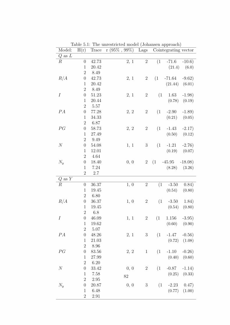
Table 5.1: The unrestricted model (Johansen approach)Model: H(r) Trace r (95% , 99%) Lags Cointegrating vectorQ as LR 0 42.73 2, 1 2 (1 -71.6 -10.6)
1 20.42 (21.4) (6.0)2 8.49
R/A 0 42.73 2, 1 2 (1 -71.64 -9.62)1 20.42 (21.44) (6.01)2 8.49
I 0 51.23 2, 1 2 (1 1.63 -1.98)1 20.44 (0.78) (0.19)2 5.57
PA 0 77.28 2, 2 2 (1 -2.90 -1.89)1 34.33 (0.21) (0.05)2 6.87
PG 0 58.73 2, 2 2 (1 -1.43 -2.17)1 27.49 (0.50) (0.12)2 9.49
N 0 54.08 1, 1 3 (1 -1.21 -2.76)1 12.01 (0.19) (0.07)2 4.64
Ny 0 18.40 0, 0 2 (1 -45.95 -18.08)1 7.24 (8.28) (3.26)2 2.7
Q as YR 0 36.37 1, 0 2 (1 -3.50 0.84)
1 19.45 (0.54) (0.80)2 6.80
R/A 0 36.37 1, 0 2 (1 -3.50 1.84)1 19.45 (0.54) (0.80)2 6.8
I 0 46.09 1, 1 2 (1 1.156 -3.95)1 19.62 (0.60) (0.90)2 5.07
PA 0 48.26 2, 1 3 (1 -1.47 -0.56)1 21.03 (0.72) (1.08)2 8.96
PG 0 83.56 2, 2 1 (1 -1.10 -0.26)1 27.99 (0.40) (0.60)2 6.20
N 0 33.42 0, 0 2 (1 -0.87 -1.14)1 7.58 (0.25) (0.33)2 2.95
Ny 0 20.87 0, 0 3 (1 -2.23 0.47)1 6.48 (0.77) (1.00)2 2.91
82

Table 5.2: Critical values of the trace-testCritical values 90 % 95 % 99 %
r=0 32.25 35.07 40.78r=1 17.98 20.16 24.69r=2 7.6 9.14 12.53
Table 5.3: The semi-endogenous model (S2S approach)Model Wald test p-value Lags (levels) Cointegrating vectorQ as LR 11.2 0.001 2 (1 0 -4.35)
(0.33)R/A 11.2 0.001 2 (1 0 -3.35)
(0.33)I 4.3 0.037 2 (1 0 -2.29)
(0.11)PA 193.9 0.000 2 (1 0 -1.32)
(0.07)PG 8.4 0.004 2 (1 0 -1.90)
(0.08)N 38.7 0.000 3 (1 0 -2.45)
(0.05)Ny 30.8 0.000 2 (1 0 -2.70)
(0.15)Q as YR 57.7 0.000 2 (1 0 -4.39)
(0.16)R/A 42.7 0.000 2 (1 0 -3.39)
(0.16)I 3.7 0.055 2 (1 0 -2.32)
(0.11)PA 4.2 0.042 3 (1 0 -1.45)
(0.12)PG 7.7 0.006 1 (1 0 -1.88)
(0.08)N 12.0 0.001 2 (1 0 -2.27)
(0.05)Ny 8.4 0.004 3 (1 0 -2.50)
(0.15)
83

Table 5.4: The Schumpeterian model (S2S approach)Model Wald test p-value LagsQ as LR 11.26 0.0036 2R/A 11.60 0.0030 2I 422.44 0.0000 2PA 2174.99 0.0000 2PG 704.80 0.0000 2N 3808.87 0.0000 3Ny 34.72 0.0000 2Q as YR 579.82 0.0000 2R/A 263.43 0.0000 2I 59.40 0.0000 2PA 1.40 0.4961 3PG 30.04 0.0000 1N 491.85 0.0000 2Ny 63.15 0.0000 3
84

Chapter 6
Conclusions
This study aims at answering the question: Has R&D had an effect on Finnishproductivity growth already since the 1950’s? The question is relevant since Finlandhas experienced high TFP growth for decades, but only the growth during the ICT-era has been studied from the point of view of R&D.
Our results show that Finnish TFP growth has followed a framework suggestedby R&D-based growth theories. Contradictory to many recent studies, the semi-endogenous growth model fits better the Finnish data than the Schumpeterianmodel. Thus is seems that for the Finnish case, increasing R&D input is needed tosustain a constant growth rate of TFP.
The Schumpeterian model implies that a constant level of R&D intensity, theidea that as the economy grows, R&D input is diluted to a larger number of sectors,generates constant growth in steady state. In steady state the constant level ofR&D intensity is obtained by having R&D input and product variety growing inlockstep. This assumption is clearly rejected in this study, but are unable to rejectthe hypothesis that product variety has some kind of role.
One might therefore think that a simple and evident extension of this work wouldbe to estimate the Schumpeterian model outside its steady state, so that R&Dinput and product proliferation are not assumed to grow strictly proportionately.
85

However, the underlying theoretical articles do not support this idea, instead theusual assumption of a steady long-run growth rate implying a balanced growthpath, is taken as given. Also having strong evidence for the semi-endogenous modelundermines the relevance of this task.
A benefit of the semi-endogenous model is that it provides an explanation to thepossibility that Finnish growth has not been on a balanced growth path throughoutthe whole time span of the study. We have a reason to assume so, due to extremedepression in early 90’s. Therefore, the result obtained could also mean that thesemi-endogenous model does hold but that the economy has been on a "constantgrowth path" as suggested by Jones (2002).
We will thus conclude that whether or not the economy was on a balanced growthpath during the timespan of the study, the semi-endogenous model fits the Finnishdata better than the Schumpeterian model.
Our results of the models are formally comparable since they are estimated asnested models. Therefore an important and useful extension to the empirical liter-ature of R&D-based endogenous growth would be to update the previous researchconducted on the U.S., OECD, etc, with this statistically sophisticated framework.
Our dataset is collected and combined from various resources and has a longertime span than many other studies of Finnish productivity. Useful results could beobtained if a measure of human capital was added to the dataset. Also, if one day thehistorical trade statistics will be available on a digital form, it could be interestingto construct a more complex measure of high technology imports. A sectoral studywith this time span would shed more light on how R&D exactly affects growth, andit would be interesting to find out which sectors in the economy have benefited mostfrom R&D in productivity terms throughout the decades.
Finally, since Finland has benefited from R&D before being in the world tech-nology frontier, it could be interesting to study whether or not these type of growthmodels, with R&D input being both domestic and foreign, are relevant in countriesthat are currently lagging behind.
86
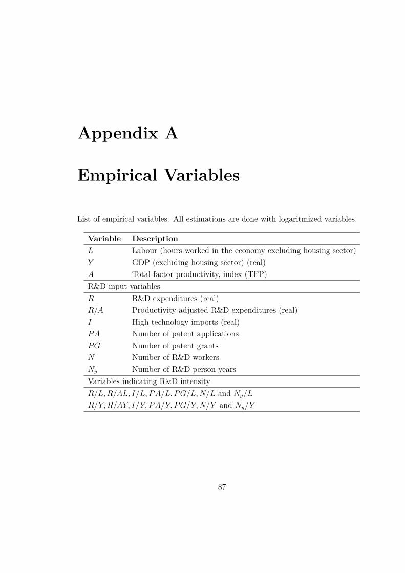
Appendix A
Empirical Variables
List of empirical variables. All estimations are done with logaritmized variables.
Variable DescriptionL Labour (hours worked in the economy excluding housing sector)Y GDP (excluding housing sector) (real)A Total factor productivity, index (TFP)R&D input variablesR R&D expenditures (real)R/A Productivity adjusted R&D expenditures (real)I High technology imports (real)PA Number of patent applicationsPG Number of patent grantsN Number of R&D workersNy Number of R&D person-yearsVariables indicating R&D intensityR/L,R/AL, I/L, PA/L, PG/L,N/L and Ny/L
R/Y,R/AY, I/Y, PA/Y, PG/Y,N/Y and Ny/Y
87

Appendix B
Unit Root Tests
Table B.1: Unit root testsVariable A L Ymodel drift & trend drift drift & trendLags (differences) 1 2 1ADF test statistic -2.38 -1.65 -2.48Residual diagnostics:Portmonteau test (2 lags) 0.33 0.31 1.51p-value 0.85 0.86 0.47ARCH-LM test (2 lags) 5.69 3.01 3.22p-value 0.06 0.22 0.20Jarque-Bera test 3.60 4.98 2.66p-value 0.16 0.08 0.26Critical values 1 % 5 % 10 %Model with drift -3.43 -2.86 -2.57Model with drift & trend -3.96 -3.41 -3.13
Critical values are from Davidson & MacKinnon (1993, p. 708).
88

Appendix C
Residual Diagnostics
The test for autocorrelation is Breusch-Godfrey LM test by Breusch (1978), Godfrey(1978) and reviewed by Godfrey (1988). Test for non-normality is from Lütkepohl(1993, p.153). Heteroscedasticity tests is a multivariate ARCH-LM test by Doornik& Hendry (1997, Sec. 10.9.2.4).
Table C.1: Residuals of the VAR modelAutocorrelation Normality Heteroscedasticity
Model test statistic p-value test statistic p-value test statistic p-valueQ as LR 14.08 0.12 10.21 0.12 19.03 0.99R/A 14.08 0.12 8.01 0.24 19.03 0.99I 11.59 0.24 11.25 0.08 40.23 0.29PA 5.41 0.80 45.36 0.00 53.80 0.03PG 7.12 0.62 49.60 0.00 46.30 0.12N 25.38 0.00 3.44 0.75 31.84 0.67Ny 16.32 0.06 9.19 0.16 18.81 0.99Q as YR 11.51 0.24 7.39 0.29 26.31 0.88R/A 11.51 0.24 5.84 0.44 26.31 0.88I 6.30 0.71 37.83 0.00 33.31 0.60PA 12.81 0.17 36.42 0.00 39.12 0.33PG 14.54 0.10 49.02 0.00 51.36 0.05N 8.67 0.47 26.46 0.00 41.07 0.26Ny 7.75 0.56 26.42 0.00 20.03 0.99
89
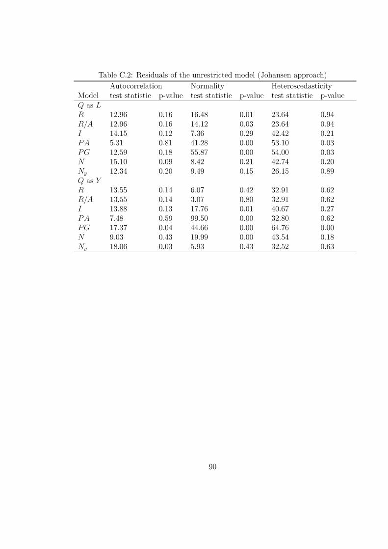
Table C.2: Residuals of the unrestricted model (Johansen approach)Autocorrelation Normality Heteroscedasticity
Model test statistic p-value test statistic p-value test statistic p-valueQ as LR 12.96 0.16 16.48 0.01 23.64 0.94R/A 12.96 0.16 14.12 0.03 23.64 0.94I 14.15 0.12 7.36 0.29 42.42 0.21PA 5.31 0.81 41.28 0.00 53.10 0.03PG 12.59 0.18 55.87 0.00 54.00 0.03N 15.10 0.09 8.42 0.21 42.74 0.20Ny 12.34 0.20 9.49 0.15 26.15 0.89Q as YR 13.55 0.14 6.07 0.42 32.91 0.62R/A 13.55 0.14 3.07 0.80 32.91 0.62I 13.88 0.13 17.76 0.01 40.67 0.27PA 7.48 0.59 99.50 0.00 32.80 0.62PG 17.37 0.04 44.66 0.00 64.76 0.00N 9.03 0.43 19.99 0.00 43.54 0.18Ny 18.06 0.03 5.93 0.43 32.52 0.63
90

Table C.3: Residuals of the semi-endogenous modelAutocorrelation Normality Heteroscedasticity
Model test statistic p-value test statistic p-value test statistic p-valueQ as LR 9.23 0.42 9.85 0.13 26.78 0.87R/A 9.23 0.42 7.32 0.29 26.78 0.87I 4.08 0.91 7.36 0.29 42.51 0.21PA 1.22 0.99 11.18 0.08 75.39 0.00PG 5.19 0.82 36.99 0.00 50.14 0.06N 6.75 0.66 13.17 0.04 28.62 0.80Ny 25.79 0.00 16.01 0.01 16.14 0.99Q as YR 6.46 0.69 4.56 0.60 38.27 0.37R/A 6.46 0.69 3.70 0.72 38.27 0.37I 33.69 0.00 35.16 0.00 34.08 0.56PA 4.75 0.86 69.81 0.00 33.69 0.58PG 6.74 0.66 26.85 0.00 61.33 0.01N 3.20 0.96 24.01 0.00 38.28 0.37Ny 11.69 0.23 12.22 0.06 34.05 0.56
Table C.4: Residuals of the Schumpeterian modelAutocorrelation Normality Heteroscedasticity
Model test statistic p-value test statistic p-value test statistic p-valueQ as LR 987.2 0.00 5.11 0.53 29.11 0.79R/A 987.2 0.00 5.11 0.53 29.11 0.79I 11430.9 0.00 13.85 0.03 44.83 0.15PA 542.7 0.00 14.28 0.03 72.20 0.00PG 23431.9 0.00 13.99 0.03 52.80 0.04N 12023.6 0.00 6.82 0.34 51.72 0.04Ny 6480.2 0.00 8.26 0.22 39.58 0.31Q as YR 334.5 0.00 8.14 0.23 60.59 0.01R/A 83.9 0.00 2.38 0.88 53.17 0.03I 403.0 0.00 10.79 0.10 38.41 0.36PA 2.7 0.98 95.28 0.00 31.36 0.69PG 50.2 0.00 26.83 0.00 63.63 0.00N 1358.8 0.00 3.85 0.70 49.48 0.07Ny 56.3 0.00 25.95 0.00 38.20 0.37
91

Appendix D
SITC-classifications
The SITC-classifications used for high technology imports, I.
• 2002–2008 SITC Revision 4
54 Medicinal and pharmaceutical products71 Power-generating machinery and equipment73 Metalworking machinery75 Office machines and automatic data-processing machines76 Telecommunications and sound-recording and reproducing apparatus and
equipment77 Electrical machinery, apparatus and appliances, n.e.s., and electrical parts
thereof (including non-electrical counterparts, n.e.s., of electrical household-type equipment)
79 Other transport equipment87 Professional, scientific and controlling instruments and apparatus, n.e.s.88 Photographic apparatus, equipment and supplies and optical goods, n.e.s.;
watches and clocks
• 1986–2001 SITC Revision 3
54 Medicinal and pharmaceutical products
92

71 Power generating machinery and equipment73 Metal working machinery75 Office machines and automatic data processing machines76 Telecommunications and sound recording and reproducing apparatus and
equipment77 Electrical machinery, apparatus and appliances, n.e.s., and electrical parts
thereof (including non-electrical counterparts, n.e.s., of electrical house-hold type equipment)
79 Other transport equipment87 Professional, scientific and controlling instruments and apparatus, n.e.s.88 Photographic apparatus, equipment and supplies and optical goods, n.e.s.;
watches and clocks
• 1976–1985 SITC Revision 2
54 Medicinal and pharmaceutical products71 Power generating machinery and equipment73 Metalworking machinery75 Office machines and automatic data processing equipment76 Telecommunications and sound recording and reproducing apparatus and
equipment77 Electrical machinery, apparatus and appliances, n.e.s., and electrical parts
thereof (including non-electrical counterparts, n.e.s., of electrical house-hold type equipment)
79 Other transport equipment87 Professional, scientific and controlling instruments and apparatus, n.e.s.88 Photographic apparatus, equipment and supplies and optical goods, n.e.s.;
watches and clocks
• 1962–1975 SITC Revised
54 Medicinal and pharmaceutical products
93

72 Electrical machinery, apparatus and appliances73 Transport equipment86 Professional, scientific and controlling instruments, photographic and op-
tical goods, watches and clocks
• 1955–1961 SITC (Original)
511 Inorganic chemicals713 Tractors other than steam721 Electric machinery, apparatus and appliances732 Road motor vehicles734 Aircraft735 Ships and boats861 Scientific, medical, optical, measuring and controlling instruments and
apparatus
94

References
Aghion, Philippe & Howitt, Peter (1992), ”A Model of Growth Through CreativeDestruction”, Econometrica, Vol. 60, No. 2, p. 323–351.
Aghion, Philippe & Howitt, Peter (1998), ”Endogenous Growth Theory”, Cam-bridge, MA:MIT Press.
Ahn, Sung K. & Reinsel, Gregory C. (1990), ”Estimation for Partially Nonsta-tionary Multivariate Autoregressive Models”, Journal of the American StatisticalAssociation, Vol. 85, No. 411, p. 813–823.
Arrow, Kenneth J. (1962), ”The Economic Implications of Learning by Doing”, TheReview of Economic Studies, Vol. 29, No. 3, p. 155–173.
Bernanke, Ben S. & Gürkaynak, Refet S. (2001), ”Is Growth Exogenous? TakingMankiw, Romer,and Weil Seriously”, NBER Book Series NBER MacroeconomicsAnnual 2001, Volume 16, p. 11–72.
Breusch, T. S. (1978), ”Testing for autocorrelation in dynamic linear models”, Aus-tralian Economic Papers, 17, p. 334–355.
Caballero, R. J. & Jaffe, A. B. (1993), ”How high are the giants’ shoulders: Anempirical assessment of knowledge spillovers and creative destruction in a modelof economic growth.”, NBER Macroeconomics Annual 1993, Volume 8, p. 15–86.
Coe, David T. & Helpman, Elhanan (1995), ”International R&D spillovers”, Euro-pean Economic Review, Vol. 39, p. 859–897.
95

Coe, David T.; Helpman, Elhanan & Hoffmaister Alexander W. (2009), ”Inter-national R&D Spillovers and Institutions”, European Economic Review 53, p.723–741.
Customs Information Service (Tullihallitus) Uljas Database (2011), www.tulli.fi/
fi/suomen_tulli/ulkomaankauppatilastot/uljas/index.jsp
Customs Information Service (Tullihallitus) Statistical Yearbooks (1955–1986),Archives of the Customs Information Service, [email protected]
Daveri, Francesco, & Silva, Olmo (2004), ”Not only Nokia: what Finland tells usabout new economy growth.” Economic Policy p. 117–163.
Davidson, R. & MacKinnon, J. (1993), ”Estimation and Inference in Econometrics”Oxford University Press.
Dinopoulos, Elias, & Thompson, Peter (1998), ”Schumpeterian Growth withoutScale Effects.” Journal of Economic Growth, 3, p. 313–335.
Doornik, J. A., & Hendry, D. F. (1997), ”Modelling Dynamic Systems Using PcFiml9.0 for Windows.” International Thomson Business Press, London.
Godfrey, L. G. (1978), ”Testing for higher order serial correlation in regression equa-tions when the regressors include lagged dependent variables.” Econometrica, 46,p. 1303–1313.
Godfrey, L. G. (1988), ”Misspecification Tests in Econometrics” Cambridge Univer-sity Press.
Griliches, Zvi (1990), ”Patent statistics as economic indicators: A survey.” NBERbook : R&D and Productivity: The Econometric Evidence, University of ChicagoPress (1998), p. 287–343.
Grossman, Gene M. & Helpman, Elhanan (1991), ”Quality Ladders in the Theoryof Growth.” The Review of Economic Studies, Vol. 58, No. 1, p. 43–61.
96

Ha, Joonkyung & Howitt, Peter (2007), ”Accounting for Trends in Productivity andR&D: A Schumpeterian Critique of Semi-Endogenous Growth Theory.”, Journalof Money, Credit and Banking Vol. 39, No.4. p. 733–774.
Hjerppe, Riitta (2008), ”An Economic History of Finland”, EH.Net Encyclopedia,edited by Robert Whaples. http://eh.net/encyclopedia/article/hjerppe.
finland
Howitt, Peter (1999), ”Steady Endogenous Growth with Population and R&D In-puts Growing.”, The Journal of Political Economy, Vol. 107, No. 4, p. 715–730.
Jalava, Jukka; Heikkinen, Sakari & Hjerppe, Riitta (2002), ”Technology and Struc-tural Change: Productivity in the Finnish Manufacturing Industries, 1925–2000.”,Transformation, Integration and Globalization Economic Research (TIGER),Working Paper No. 34.
Jalava, Jukka & Pohjola, Matti (2007), ”ICT as a Source of Output and ProductivityGrowth in Finland”, Telecommunications Policy, 31, p. 463–472.
Jalava, Jukka & Pohjola, Matti (2008), ”The Roles of Electricity and ICT in Eco-nomic Growth: Case Finland.”, Explorations in Economic History, 45, p. 270–287.
Jalava, Jukka; Pohjola, Matti; Ripatti, Antti & Vilmunen, Jouko (2006), ”BiasedTechnical Change and Capital–Labour Substitution in Finland, 1902–2003.”, Top-ics in Macroeconomics , Vol. 6, Iss. 1, Art. 8.
Johansen, Søren (1988), ”Statistical Analysis of Cointegration Vectors”, Journal ofEconomic Dynamics and Control, 12, p. 231–254.
Johansen, Søren & Juselius, Katarina (1990), ”Maximum Likelihood Estimationand Inference on Cointegration —with Applications to the Demand for Money”,Oxford Bulletin of Economics and Statistics, 52, 2, p. 169–210.
97
Johansen, Søren (1991), ”Estimation and Hypothesis Testing of Cointegration Vec-tors in Gaussian Vector Autoregressive Models”, Econometrica, Vol. 59, No. 6,p. 1551–1580.
Johansen, Søren (1995), ”Likelihood-based Inference in Cointegrated Vector Autore-gressive Models, Advanced Texts in Econometrics”, Oxford University Press.
Jones, Charles I. (1995a), ”Time Series Tests of Endogenous Growth Models.”, Quar-terly Journal of Economics, 110, p. 495–525.
Jones, Charles I. (1995b) ”R&D-Based Models of Economic Growth”, Journal ofPolitical Economy, 103, p. 759–84.
Jones, Charles I. (1999) ”Growth: With or without Scale Effects?”, The AmericanEconomic Review, Vol. 89, No. 2, Papers and Proceedings of the One HundredEleventh Annual Meeting of the American Economic Association, p. 139–144.
Jones, Charles I. (2002) ”Sources of U.S. Economic Growth in a World of Ideas”,The American Economic Review, Vol. 92, No. 1, p. 220–239.
Kortum, Sam. (1997) ”Research, Patenting, and Technological Change”, Economet-rica, 65, p. 1389–1419.
Lucas, Robert E. Jr. (1988) ”On the Mechanics of Economic Development”, Journalof Monetary Economics 22, p. 3–42. North-Holland.
Lütkepohl, Helmut (1993), ”Introduction to Multiple Time Series Analysis, 2nd.edition”, Springer.
Lütkepohl, Helmut (2005), ”New Introduction to Multiple Time Series Analysis”,Springer-Verlag.
Lütkepohl, Helmut & Krätsig, Markus (2004), ”Applied Time Series Econometrics”,Cambridge University Press.
98

Madsen, Jacob B.(2008), ”Semi-endogenous versus Schumpeterian Growth Models:Testing the Knowledge Production Function Using International Data”, Journalof Economic Growth 13, p. 1–26.
Madsen, Jacob B.; Saxena, Shishir; Ang, James B. (2010), ”The Indian growthmiracle and endogenous growth”, Journal of Development Economics 93, p. 37–48.
Maliranta, Mika ; Rouvinen, Petri; Ylä-Anttila, Pekka (2010), ”Finland’s Path tothe Global Productivity Frontier through Creative Destruction”, InternationalProductivity Monitor, 20, p. 68–84.
OECD (2006), ”OECD Compendium of Productivity Indicators 2006”, http://
www.oecd.org/dataoecd/4/22/37574961.pdf
Peretto, Pietro (1998), ”Technological Change and Population Growth.”, Journal ofEconomic Growth, 3, p. 283–311.
Peretto, Pietro & Smulders, Sjak (2002), ”Technological Distance, Growth and ScaleEffects”, Economic Journal, 112, p. 603–24.
Pessoa, Argentino (2010), ”R&D and economic growth: How strong is the link?”,Economics Letters, Elsevier, vol. 107(2), p. 152–154.
Piekkola, Hannu (2007), ”Public Funding of R&D and Growth: Firm-Level Evidencefrom Finland”, Economics of Innovation and New Technology, 16:3, p. 195–210.
Rebelo, Sergio (1991), ”Long-Run Policy Analysis and Long-Run Growth”, Journalof Political Economy, Vol. 99, No. 3, p. 500–52.
Romer, Paul M. (1986), ”Increasing Returns and Long–Run Growth”, Journal ofPolitical Economy, Vol. 94, No. 5, p. 1002–1037.
Romer, Paul M. (1986), ”Growth Based on Increasing Returns Due to Specializa-tion”, The American Economic Review, Vol. 77, No. 2, Papers and Proceedings
99

of the Ninety-Ninth Annual Meeting of the American Economic Association, p.56–62.
Romer, Paul M. (1990), ”Endogenous Technological Change”, Journal of PoliticalEconomy, Vol. 98, No. 5, Part 2: The Problem of Development: A Conference ofthe Institute for the Study of Free Enterprise Systems, p. 71–102.
Saarinen, Jani (2005), ”Innovations and Industrial Performance in Finland 1945–1998”, Lund Studies in Economic History.
Schumpeter, J. A. (1942), ”Capitalism, Socialism and Democracy”, New York:Harper and Brothers.
Segerström, Paul S. (1998) ”Endogenous Growth Without Scale Effects.”, AmericanEconomic Review, 88, p. 1290–1310.
Solow, Robert M. (1956), ”A Contribution to the Theory of Economic Growth”,Quarterly Journal of Economics (The MIT Press) 70 (1) p. 65–94.
Statistics Finland (2011), http://pxweb2.stat.fi/database/StatFin/
Trajtenberg, Manuel (1990), ”A Penny for Your Quotes: Patent Citations and theValue of Innovations”, The RAND Journal of Economics, Vol.21, No.1, p. 172–187.
United Nations Statistic Division (2012), ”Detailed structure and explanatory notes,Standard International Trade Classification, Rev.4”, http://unstats.un.org/
unsd/cr/registry/regcst.asp?Cl=28
The World Intellectual Property Organization WIPO (2011), statistics: http://
www.wipo.int/ipstats/en/statistics/patents/
The World Intellectual Property Organization WIPO (2010), ”World Intel-lectual Property Indicators 2010”, http://www.wipo.int/export/sites/www/
ipstats/en/statistics/patents/pdf/941_2010.pdf
100

Young, Alwyn (1998), ”Growth Without Scale Effects.”, Journal of Political Econ-omy, 106, p. 41–63.
Zachariadis, Marios (2003), ”R&D, Innovation, and Technological Progress: a Testof the Schumpeterian Framework without Scale Effects”, Canadian Journal ofEconomics / Revue canadienne d’Economique, Vol. 36, No. 3, p. 566–586.
Zachariadis, Marios (2004), ”R&D-induced Growth in the OECD?”, Review of De-velopment Economics, 8(3), p. 423–439.
101