AbstractRAMRAKHYANI, PRAKASH SHYAMLAL

Dynamic Pipeline Scaling(Under the direction of Dr. Eric Rotenberg)

The classic problem of balancing power and performance continues to exist, as

technology progresses. Fortunately, high performance is not a constant requirement in a

system. When the performance requirement is not at its peak, the processor can be configured

to conserve power, while providing just enough performance. Parameters like voltage,

frequency, and cache structure have been proposed to be made dynamically scalable, to

conserve power. This thesis analyzes the effects of dynamically scaling a new processor

parameter, pipeline depth.

We propose Dynamic Pipeline Scaling, a technique to conserve energy at low

frequencies when voltage is invariable. When frequency can be lowered enough, adjacent

pipeline stages can be merged to form a shallow pipeline. At equal voltage and frequency, the

shallow pipeline is more energy-efficient than the deep pipeline. This is because the shallow

pipeline has fewer data dependence stalls and a lower branch misprediction penalty. Thus,

there are fewer wasteful transitions in a shallow pipeline, which translates directly to lower

energy consumption. On a variable-voltage processor, the shallow pipeline requires a higher

operating voltage than the deep pipeline for the same frequency. Since energy depends on the

square of voltage and depends linearly on the total number of transitions, on a variable-voltage

processor, a deep pipeline is typically more energy-efficient than a shallow pipeline. However,

there may be situations where variable voltage is not desired. For example, if the latency to

switch voltage is large, voltage scaling may not be beneficial in a real-time system with tight

deadlines. On such a system, dynamic pipeline scaling can yield energy benefits, in spite of not

scaling voltage.

Dynamic Pipeline Scaling

byPRAKASH SHYAMLAL RAMRAKHYANI

A thesis submitted to the Graduate Faculty ofNorth Carolina State University

in partial fulfillment of therequirements for the Degree of

Master of Science

COMPUTER ENGINEERING

Raleigh2003

Approved by

______________________Dr. Eric Rotenberg, Chair of the Advisory Committee

___________________ __________________Dr. Thomas M. Conte Dr. W. Rhett Davis

_____________________Dr. Alexander G. Dean

ii

BIOGRAPHY

Prakash Ramrakhyani was born on the 29th of July 1979. In June 2000, he

received his Bachelors degree in Electronics Engineering from the University of Mumbai,

at Mumbai, India. From November 2000 to July 2001, he worked as a Systems Engineer

for the Optical Networks Unit in Wipro Technologies at Bangalore, India.

He enrolled at the North Carolina State University, Raleigh in August 2001, to

work towards a Masters degree in Computer Engineering. In July 2002, he joined Dr.

Rotenberg’s research group in the Department of Electrical and Computer Engineering

and has been working under his guidance since then.

iii

Acknowledgements

First and foremost I would like to thank my parents, Mr. Shyamlal Ramrakhyani

and Mrs. Lata Ramrakhyani, for their continuous support against every challenge that I

have faced in my life. My brother, Deepak Ramrakhyani, would be second on the list. He

is not only a great brother but the best buddy that I have ever had. The patient person that

my brother is, he is so because he figured early in his life, a way to tolerate all my

idiosyncrasies and still love me dearly.

I am not sure if I could ever sum up what I owe Dr. Eric Rotenberg, my academic

advisor. The word ‘guru’, which is popularly used to refer to an expert, is derived from

the ancient Indian language, Sanskrit. In Sanskrit it is used to denote a person who is not

just an expert but also a teacher and a guide, who is committed to the welfare of his

advisees. Dr. Rotenberg has influenced me a lot. Try as I may, I will never be able to

emulate him completely. He has been a true ‘guru’ to me and I thank him for being so.

Thanks are due to all the members of Dr. Rotenberg’s research group Zach,

Karthik, Nikhil, Aravindh, Ravi Vekatesan, Ahmed, and Ali. It has been just great to be a

part of the group. I should make a special reference to Jinson, who ceased to be a part of

the group when I joined it, but made himself available, whenever I required his help.

Thank you, Jinson. Thank you, Nikhil and Aravindh, for being such great pals and

providing with much needed breaks from research.

I am grateful to the many friends I made at graduate school; Adi, Ashish, Pushkar,

Praveen, Ravi Rajagopalan, Subhayu, Rohit, Rahul, Vishal, Shivjit, Abhishek, Puneet, …

and many more, for their companionship and help in many different ways. I will never

forget the wonderful dinner gatherings that we had at Nikhil’s along with Viraj, Vikas,

iv

Shalin, Sameer, Aditya, the two Rachanas, Jayanthi, Magadhi, Shalini, and the rest of the

gang. Thank you, Ben and Mark for co-developing with me, the prototype of the EDF-

scheduler that has been used for this thesis.

I would like to thank Dr. Thomas Conte, Dr. Alexander Dean and Dr. Rhett Davis

for having accepted to be the members of my advisory committee.

This material is based upon work supported by the National Science

Foundation under Grant No. 0207785. Special thanks are due to Intel for

generous funding and equipment donations.

v

TABLE OF CONTENTS

LIST OF FIGURES .......................................................................................................... vii

LIST OF TABLES.............................................................................................................. x

Chapter 1 Introduction ........................................................................................................ 1

1.1 Contributions ............................................................................................................ 3

1.2 Organization.............................................................................................................. 4

Chapter 2 Related Work...................................................................................................... 5

Chapter 3 Dynamic Pipeline Scaling .................................................................................. 7

Chapter 4 Design Techniques for DPS-enabled Pipeline Stages...................................... 11

4.1 Pipeline stages for shallow and deep modes........................................................... 11

4.2 Techniques for deep pipelining and dynamic pipeline scaling............................... 12

4.2.1 Techniques for memory/cache structures ........................................................ 13

4.2.2 Instruction fetch ............................................................................................... 13

4.2.3 Register renaming ............................................................................................ 13

4.2.4 Issue logic ........................................................................................................ 16

4.2.5 Execute stage ................................................................................................... 20

Chapter 5 Simulation Methodology.................................................................................. 25

5.1 Cycle-accurate simulator ........................................................................................ 25

5.2 Power modeling in cycle-accurate simulator.......................................................... 26

5.3 EDF scheduler simulator and frequency scaling algorithm.................................... 27

Chapter 6 Results .............................................................................................................. 32

6.1 Experiments with the cycle-accurate processor simulator...................................... 32

6.1.1 Comparison of energy consumption on a fixed-voltage processor.................. 32

6.1.2 Comparison of energy consumption on a variable-voltage processor ............. 39

vi

6.2 Experiments using the EDF scheduler.................................................................... 44

Chapter 7 Summary and Future Work .............................................................................. 54

References......................................................................................................................... 55

vii

LIST OF FIGURES

Figure 3-1. Dynamic Pipeline Scaling. ............................................................................... 7

Figure 3-2. Frequency range of deep and shallow modes. ................................................. 7

Figure 3-3. V-f characteristic of variable-voltage processor for two pipeline depths. ....... 8

Figure 4-1. Description of pipeline modes. ...................................................................... 11

Figure 4-2. Single-cycle rename logic. ............................................................................. 14

Figure 4-3. Two–cycle rename logic. ............................................................................... 15

Figure 4-4. Comparing single-cycle and two-cycle issue................................................. 17

Figure 4-5. Two-cycle issue with select-free scheduling [4]............................................ 18

Figure 4-6. Two-stage adder for deep mode..................................................................... 21

Figure 4-7. Comparing half-word and full-word bypasses............................................... 21

Figure 4-8. Single-stage adder for shallow mode. ............................................................ 22

Figure 4-9. Modified issue logic for deep mode............................................................... 23

Figure 4-10. Modified issue logic for shallow mode........................................................ 24

Figure 6-1. Comparison of energy consumption by a rigid-deep pipeline v/s a DPS-enabled pipeline on a fixed-voltage processor for bzip. ........................................... 33

Figure 6-2. Comparison of energy consumption by a rigid-deep pipeline v/s a DPS-enabled pipeline on a fixed-voltage processor for gap. ............................................ 33

Figure 6-3. Comparison of energy consumption by a rigid-deep pipeline v/s a DPS-enabled pipeline on a fixed-voltage processor for gcc.............................................. 34

Figure 6-4. Comparison of energy consumption by a rigid-deep pipeline v/s a DPS-enabled pipeline on a fixed-voltage processor for gzip. ........................................... 34

Figure 6-5. Comparison of energy consumption by a rigid-deep pipeline v/s a DPS-enabled pipeline on a fixed-voltage processor for mcf. ............................................ 35

Figure 6-6. Comparison of energy consumption by a rigid-deep pipeline v/s a DPS-enabled pipeline on a fixed-voltage processor for parser. ........................................ 35

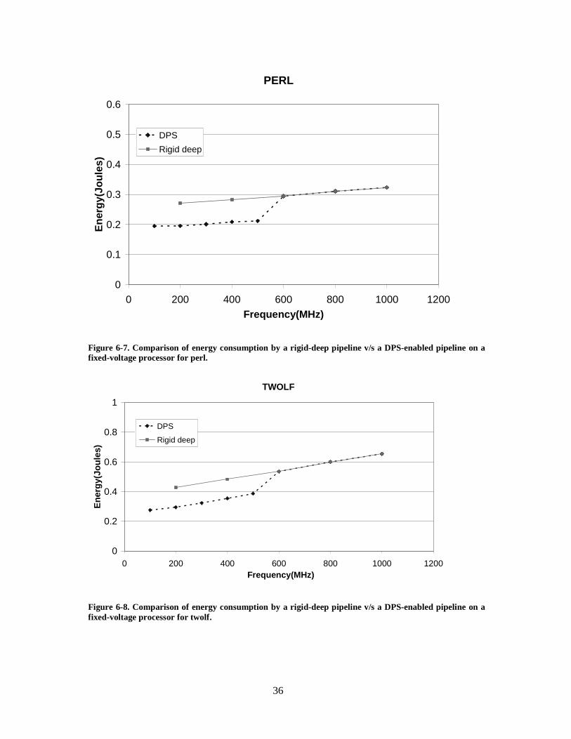
Figure 6-7. Comparison of energy consumption by a rigid-deep pipeline v/s a DPS-enabled pipeline on a fixed-voltage processor for perl. ............................................ 36

viii

Figure 6-8. Comparison of energy consumption by a rigid-deep pipeline v/s a DPS-enabled pipeline on a fixed-voltage processor for twolf........................................... 36

Figure 6-9. Comparison of energy consumption by a rigid-deep pipeline v/s a DPS-enabled pipeline on a fixed-voltage processor for vortex. ........................................ 37

Figure 6-10. Comparison of energy consumption by a rigid-deep pipeline v/s a DPS-enabled pipeline on a fixed-voltage processor for vpr.............................................. 37

Figure 6-11. Confirmation that energy difference between shallow and deep modes is dueto wasteful transitions. .............................................................................................. 38

Figure 6-12. Comparison of energy consumption by a rigid-deep pipeline v/s a DPS-enabled pipeline on a variable-voltage processor for bzip........................................ 39

Figure 6-13. Comparison of energy consumption by a rigid-deep pipeline v/s a DPS-enabled pipeline on a variable-voltage processor for gap......................................... 40

Figure 6-14. Comparison of energy consumption by a rigid-deep pipeline v/s a DPS-enabled pipeline on a variable-voltage processor for gcc. ........................................ 40

Figure 6-15. Comparison of energy consumption by a rigid-deep pipeline v/s a DPS-enabled pipeline on a variable-voltage processor for gzip........................................ 41

Figure 6-16. Comparison of energy consumption by a rigid-deep pipeline v/s a DPS-enabled pipeline on a variable-voltage processor for mcf. ....................................... 41

Figure 6-17. Comparison of energy consumption by a rigid-deep pipeline v/s a DPS-enabled pipeline on a variable-voltage processor for parser..................................... 42

Figure 6-18. Comparison of energy consumption by a rigid-deep pipeline v/s a DPS-enabled pipeline on a variable-voltage processor for perl. ....................................... 42

Figure 6-19. Comparison of energy consumption by a rigid-deep pipeline v/s a DPS-enabled pipeline on a variable-voltage processor for twolf. ..................................... 43

Figure 6-20. Comparison of energy consumption by a rigid-deep pipeline v/s a DPS-enabled pipeline on a variable-voltage processor for vortex. ................................... 43

Figure 6-21. Comparison of energy consumption by a rigid-deep pipeline v/s a DPS-enabled pipeline on a variable-voltage processor for vpr. ........................................ 44

Figure 6-22. Ratio of shallow-mode IPC to deep-mode IPC............................................ 45

Figure 6-23. Energy consumption for different processor models for task sets withcharacteristics similar to bzip and worst-case utilization equal to 1......................... 47

Figure 6-24. Energy consumption for different processor models for task sets withcharacteristics similar to gap and worst-case utilization equal to 1.......................... 48

ix

Figure 6-25. Energy consumption for different processor models for task sets withcharacteristics similar to the pseudo benchmark and worst-case utilization equal to 1.................................................................................................................................... 48

Figure 6-26. Energy consumption for different processor models for task sets withcharacteristics similar to bzip and worst-case utilization equal to 0.5...................... 49

Figure 6-27. Energy consumption for different processor models for task sets withcharacteristics similar to gap and worst-case utilization equal to 0.5....................... 49

Figure 6-28. Energy consumption for different processor models for task sets withcharacteristics similar to the pseudo benchmark and worst-case utilization equal to0.5.............................................................................................................................. 50

Figure 6-29. Distribution of CPU time for task sets with characteristics similar to bzipand worst-case utilization of 1. ................................................................................. 50

Figure 6-30. Distribution of CPU time for task sets with characteristics similar to gap andworst-case utilization of 1. ........................................................................................ 51

Figure 6-31. Distribution of CPU time for task sets with characteristics similar to thepseudo benchmark and worst-case utilization of 1. .................................................. 51

Figure 6-32. Distribution of CPU time for task sets with characteristics similar to bzipand worst-case utilization of 0.5. .............................................................................. 52

Figure 6-33. Distribution of CPU time for task sets with characteristics similar to gap andworst-case utilization of 0.5. ..................................................................................... 52

Figure 6-34. Distribution of CPU time for task sets with characteristics similar to thepseudo benchmark and worst-case utilization of 0.5. ............................................... 53

x

LIST OF TABLES

Table 4-1. PISA instructions that can produce/consume lower half-word early. ............. 22

Table 5-1. Processor configuration. .................................................................................. 25

Table 5-2. Voltage-frequency pairs for shallow and deep modes. ................................... 26

Table 5-3. Power consumed in different modes on a variable-voltage processor, for thegap benchmark. ......................................................................................................... 26

Table 5-4. Power consumed in different modes on a variable-voltage processor, for thebzip benchmark. ........................................................................................................ 27

Table 5-5. Power consumed on a fixed-voltage processor, for the gap and bzipbenchmarks. .............................................................................................................. 27

1

Chapter 1 Introduction

The undiminishing need to improve performance has caused transistor density and

power to increase significantly. However, to keep temperature of the chip within limits,

power density of the chip needs to be maintained at a reasonable level. The conflict between

power and performance has led architects to make design decisions “on-the-fly”. To balance

power and performance, design parameters that were earlier supposed to be fixed once a chip

was shipped, such as voltage, frequency, and even cache structure, are now being considered

variable. This thesis attempts to analyze the effects of making a new design parameter

variable, namely pipeline depth. We have discovered that pipeline depth impacts

power/energy by affecting the amount of useless switching activity. This observation is at the

core of this thesis. Dynamic pipeline scaling is a new microarchitecture substrate for tuning

the amount of useless switching activity by scaling pipeline depth with frequency.

Power consumed by a processor can be broken into dynamic power and static power.

Static power is attributed to leakage and sub-threshold currents in the circuit. Dynamic power

is the power consumed due to switching. It can be expressed as the power required to

charge/discharge a capacitor. In present day circuits, dynamic power forms the bulk of total

power consumed. A lot of research effort is being spent on reducing dynamic power and

energy related to dynamic power. Techniques like dynamic voltage scaling, clock gating, and

fetch gating have been proposed to reduce dynamic power.

The expression for dynamic power is given by the relation

fVCP 2 ⋅⋅⋅α= ... 1.1

whereÿ is the switching factor (defined as the number of transitions per unit time), C is the

amount of switched capacitance, V is the applied voltage, and f is the frequency of operation.

2

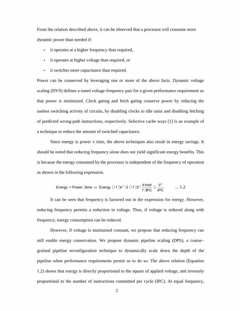
From the relation described above, it can be observed that a processor will consume more

dynamic power than needed if:

• it operates at a higher frequency than required,

• it operates at higher voltage than required, or

• it switches more capacitance than required.

Power can be conserved by leveraging one or more of the above facts. Dynamic voltage

scaling (DVS) defines a tuned voltage-frequency pair for a given performance requirement so

that power is minimized. Clock gating and fetch gating conserve power by reducing the

useless switching activity of circuits, by disabling clocks to idle units and disabling fetching

of predicted wrong-path instructions, respectively. Selective cache ways [1] is an example of

a technique to reduce the amount of switched capacitance.

Since energy is power x time, the above techniques also result in energy savings. It

should be noted that reducing frequency alone does not yield significant energy benefits. This

is because the energy consumed by the processor is independent of the frequency of operation

as shown in the following expression.

ÿ⋅= timePowerEnergyIPCV

IPCfinstr#

VftVfEnergy2

22 ∝⋅

⋅∝⋅⋅∝ ... 1.2

It can be seen that frequency is factored out in the expression for energy. However,

reducing frequency permits a reduction in voltage. Thus, if voltage is reduced along with

frequency, energy consumption can be reduced.

However, if voltage is maintained constant, we propose that reducing frequency can

still enable energy conservation. We propose dynamic pipeline scaling (DPS), a coarse–

grained pipeline reconfiguration technique to dynamically scale down the depth of the

pipeline when performance requirements permit us to do so. The above relation (Equation

1.2) shows that energy is directly proportional to the square of applied voltage, and inversely

proportional to the number of instructions committed per cycle (IPC). At equal frequency,

3

shallow pipelines have higher IPC than deep pipelines due to fewer data stall cycles and

lower branch misprediction penalties. These two factors translate to less useless switching

activity, as we will explain in more detail later in Chapter 3. For frequencies within the

operating range of the shallow pipeline, switching to the shallow pipeline can provide a one-

time energy benefit over the deep pipeline due to less useless switching activity.

On a variable-voltage processor, the voltage required to operate a deep pipeline at the

lower frequency is less than the voltage required to operate a shallow pipeline. Since energy

has a quadratic relation with voltage and only a linear inverse relation with IPC, the deep

pipeline tends to be more power and energy efficient than the shallow pipeline due to lower

operating voltage on the variable-voltage processor. However, there may be several situations

that make voltage variability undesirable or infeasible. These may include but are not limited

to

• process technology,

• voltage switching latency, and

• design/verification complexity.

For the PXA250, one of Intel’s latest DVS-enabled processors, the maximum latency

for the applied voltage to stabilize after a change is specified to be beyond 10 milliseconds

[7]. This latency may be too large for a system which has a number of fine-grained tasks with

real-time deadlines. DPS provides an alternative solution in such a scenario. However, a

detailed analysis of the limited applicability of DVS is left for future work. The primary

purpose of this thesis is to study the power/energy impact of pipeline depth and develop a

microarchitecture that permits scaling the pipeline depth dynamically.

1.1 Contributions

• This thesis proposes Dynamic Pipeline Scaling (DPS), a scheme for power and energy

reduction in processors where variable voltage is not desired or achievable.

4

• This thesis explains the fundamental differences in energy consumption of a deep

pipeline versus a shallow pipeline. An understanding of these differences forms the

basis of the proposed scheme.

• Methods for designing DPS-enabled pipeline stages were developed.

• An EDF-based task scheduling simulator, embedded with a frequency scaling

algorithm, was developed. A prototype of this was developed as part of a course

project. However, significant enhancements were made, such as ensuring safety in

spite of multiple pre-emptions, estimating energy consumption, modeling overhead

due voltage switching, and modeling DPS.

• Wattch power models were integrated into a cycle-accurate DPS-enabled processor

simulator. This enabled measuring power and energy of the processor with different

operating modes and quantifying the benefits of the proposed scheme.

1.2 Organization

Chapter 2 provides a review of existing power-management techniques for

processors. Chapters 3 and 4 are the main contribution of this thesis. Chapter 3 explains the

idea of dynamic pipeline scaling, the benefits of dynamic pipeline scaling, and how these

benefits are obtained. In particular, we explain that power efficiency of shallow pipelines

over deep pipelines (for constant voltage) is due to useless switching activity. Chapter 4

describes mechanisms for scaling key stages in the pipeline, including the rename stage, issue

stage, and execute stage. Chapter 5 discusses the simulation methodology and experiments

performed. Chapter 6 presents the results obtained from experiments. Chapter 7 summarizes

the thesis and discusses future work.

5

Chapter 2 Related Work

There has been a lot of work related to power-efficient design of microprocessors. A

few significant ones are discussed in this section.

The frequency of a processor can be defined by the relation

V

)VV(Kfrequency

2t−

⋅=

Thus, when V>>Vt, there exists a linear relationship between frequency and applied voltage.

Dynamic voltage scaling leverages this fact to save power. When the performance

requirement of the system is not at its peak, the frequency of the processor can be reduced.

From the relation above, it can be seen that reducing frequency allows voltage to be reduced.

Since dynamic power has a linear relationship with frequency and a quadratic relation with

voltage, dynamic voltage scaling enables a cubic savings in dynamic power and quadratic

savings in dynamic energy. Using DPS in conjunction with voltage scaling may not provide

benefits because the minimum operating voltage required for a given frequency is higher for

shallow pipelines than for deep pipelines. However, on voltage-invariable processors, DPS

provides significant energy savings. If the voltage switching latency is large, voltage scaling

may not be applicable to hard real-time systems in which switching latency is a large fraction

of or larger than the deadline. On the other hand, fast frequency switching can be achieved

[20]. For such a system, when frequency is considerably low, pipeline scaling will yield

energy savings.

Dynamic power in a system can be reduced by cutting off switching activity occurring

in portions of the circuit that are not being used. This can be done by disabling the clock

being fed to these portions during the period when they are not being used, a technique

referred to as clock gating. This technique works well during serial portions of the program,

6

as instructions wait for dependences to be resolved, leaving many parallel function units idle.

Pipeline gating [17], when used in conjunction with clock gating, helps reduce energy

consumption in programs which have high branch misprediction rates. DPS tackles both of

these situations by reducing the latencies to resolve dependences and branch mispredictions.

Selective cache ways [1] is a technique proposed by D. H. Albonesi to reduce power

consumed by caches. He proposes to dynamically reduce the number of active ways in the

cache based on how active the ways are. Disabling ways not only reduces dynamic power but

also reduces static power. This technique can be used in conjunction with dynamic pipeline

scaling to further optimize energy in a DPS-enabled processor.

Previously, we made a case for dynamic pipeline scaling with respect to potential

technology trends and their impact on the useful frequency range of DVS [14].

Several frequency scaling algorithms have been proposed [2] [9] [10] [12] [15] [16]

[23] [24] [25]. The algorithm implemented for this thesis is a combination of two previous

approaches [23] [2], enhanced with a crucial modification to ensure safety when voltage

switching latency is considerable. DPS provides an energy-saving microarchitectural

substrate for frequency scaling algorithms, when variable voltage is not desired or cannot be

used.

7

Chapter 3 Dynamic Pipeline Scaling

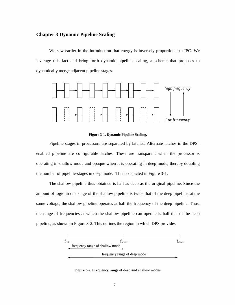
We saw earlier in the introduction that energy is inversely proportional to IPC. We

leverage this fact and bring forth dynamic pipeline scaling, a scheme that proposes to

dynamically merge adjacent pipeline stages.

Figure 3-1. Dynamic Pipeline Scaling.

Pipeline stages in processors are separated by latches. Alternate latches in the DPS–

enabled pipeline are configurable latches. These are transparent when the processor is

operating in shallow mode and opaque when it is operating in deep mode, thereby doubling

the number of pipeline-stages in deep mode. This is depicted in Figure 3-1.

The shallow pipeline thus obtained is half as deep as the original pipeline. Since the

amount of logic in one stage of the shallow pipeline is twice that of the deep pipeline, at the

same voltage, the shallow pipeline operates at half the frequency of the deep pipeline. Thus,

the range of frequencies at which the shallow pipeline can operate is half that of the deep

pipeline, as shown in Figure 3-2. This defines the region in which DPS provides

Figure 3-2. Frequency range of deep and shallow modes.

high frequency

low frequency

frequency range of deep mode

frequency range of shallow modefdmaxfmin fsmax

8

benefits to be the lower half of the frequency range in deep mode.

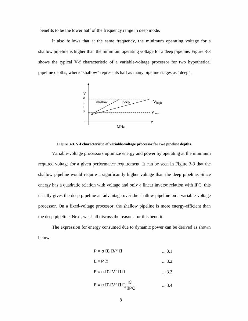
It also follows that at the same frequency, the minimum operating voltage for a

shallow pipeline is higher than the minimum operating voltage for a deep pipeline. Figure 3-3

shows the typical V-f characteristic of a variable-voltage processor for two hypothetical

pipeline depths, where “shallow” represents half as many pipeline stages as “deep”.

Figure 3-3. V-f characteristic of variable-voltage processor for two pipeline depths.

Variable-voltage processors optimize energy and power by operating at the minimum

required voltage for a given performance requirement. It can be seen in Figure 3-3 that the

shallow pipeline would require a significantly higher voltage than the deep pipeline. Since

energy has a quadratic relation with voltage and only a linear inverse relation with IPC, this

usually gives the deep pipeline an advantage over the shallow pipeline on a variable-voltage

processor. On a fixed-voltage processor, the shallow pipeline is more energy-efficient than

the deep pipeline. Next, we shall discuss the reasons for this benefit.

The expression for energy consumed due to dynamic power can be derived as shown

below.

fVCP 2 ⋅⋅⋅α= ... 3.1

tPE ⋅= ... 3.2

tfVCE 2 ⋅⋅⋅⋅α= ... 3.3

IPCfIC

fVCE 2

⋅⋅⋅⋅⋅α= ... 3.4

Volts

MHz

shallow deep Vhigh

Vlow

9

cyclesVCE 2 ⋅⋅⋅α= ... 3.5

cyclesVCcycles

stransition#E 2 ⋅⋅⋅= ... 3.6

2VCstransition#E ⋅⋅= ... 3.7

Equation 3.1 describes the relation for dynamic power. Since energy is the integral of

power over time, we can define dynamic energy to be the product of dynamic power and

time. Substituting for time using the classic performance equation [11], we get energy to be

the product of the switching factor (ÿ), the capacitance (C), the square of the operating

voltage (V), and the number of cycles it takes to execute the program. Switching factor is the

ratio of the total number of transitions and the number of cycles. Substituting forÿ in

equation 3.5, and simplifying the resulting equation, we arrive at equation 3.7.

Thus, it can be seen that the total energy consumption for executing a program is a

function of the total transitions it takes to run the program, the total capacitance in the

processor, and the voltage at which the processor is operating. It can also be seen that the

energy consumed is independent of the frequency at which the processor is operating.

The number of transitions in a program depends on the nature and size of the program

and the architecture of the processor. Thus, one of two processors running the same program

at the same voltage and frequency may consume less energy than the other because its

microarchitecture is more energy-efficient. The total number of transitions required to run a

program can be decomposed into two portions, (1) useful transitions and (2) wasteful

transitions. Useful transitions are the transitions that contribute directly to the execution of

the program and are required for correct operation. Wasteful transitions are transitions that do

not contribute towards correct execution of the program and if minimized can help reduce

power and energy. These transitions are due to data stalls and instructions fetched/executed

down the wrong path. At equal voltage and frequency of operation, a shallow pipeline is

more energy-efficient than the deep pipeline because shallow pipelines have fewer wasteful

10

transitions. This is so because shallow pipelines have fewer data dependence stalls and lower

branch misprediction penalties. The minimum branch misprediction penalty for the deep

mode is twice the minimum branch misprediction penalty for the shallow mode. The deep

pipeline fetches/executes more wrong-path instructions before resolving a mispredicted

branch.

As mentioned above, the wasteful energy in a processor is due to instructions

fetched/executed down the wrong path and switching happening in pipeline-stages that are

not actually processing any instructions due to data stalls. Perfect clock gating can help do

away with energy consumed due to data stalls. Either perfect branch prediction or perfect

fetch gating [17] will help do away with energy consumed due to instructions

fetched/executed down the wrong path. To put it in other words, with perfect clock gating

and perfect fetch gating, a deep pipeline will have the same energy as the shallow pipeline.

On a real system, however, this is not achievable. Dynamic pipeline scaling reduces the

inefficiencies of a deep pipeline by dynamically switching to a shallow pipeline, when the

performance requirements permit the microarchitecture to do so.

11

Chapter 4 Design Techniques for DPS-enabled Pipeline Stages

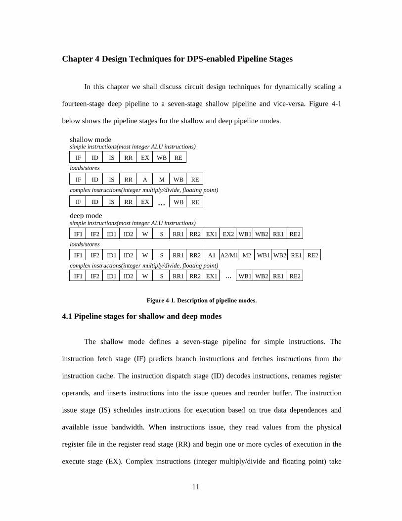
In this chapter we shall discuss circuit design techniques for dynamically scaling a

fourteen-stage deep pipeline to a seven-stage shallow pipeline and vice-versa. Figure 4-1

below shows the pipeline stages for the shallow and deep pipeline modes.

Figure 4-1. Description of pipeline modes.

4.1 Pipeline stages for shallow and deep modes

The shallow mode defines a seven-stage pipeline for simple instructions. The

instruction fetch stage (IF) predicts branch instructions and fetches instructions from the

instruction cache. The instruction dispatch stage (ID) decodes instructions, renames register

operands, and inserts instructions into the issue queues and reorder buffer. The instruction

issue stage (IS) schedules instructions for execution based on true data dependences and

available issue bandwidth. When instructions issue, they read values from the physical

register file in the register read stage (RR) and begin one or more cycles of execution in the

execute stage (EX). Complex instructions (integer multiply/divide and floating point) take

WIF1 IF2 ID1 ID2 S RR1 WB2RR2 EX1 EX2 WB1 RE1 RE2

EXIF ID IS RR WB RE

AIF ID IS RR REWBM

IF ID IS RR REWB…EX

WIF1 IF2 ID1 ID2 S RR1 WB2RR2 A1 M2 WB1 RE1 RE2A2/M1

WIF1 IF2 ID1 ID2 S RR1 WB2RR2 … WB1 RE1 RE2EX1

shallow mode

deep mode

simple instructions(most integer ALU instructions)

loads/stores

complex instructions(integer multiply/divide, floating point)

loads/stores

simple instructions(most integer ALU instructions)

complex instructions(integer multiply/divide, floating point)

12

more than one cycle to execute. In place of the EX stage, loads and stores go through the

address generation stage (A) followed by the cache access stage (M). Following execution or

accessing the cache, values are written into the register file and bypassed to dependent

instructions in the writeback stage (WB). Instructions are retired from the reorder buffer in

the retire stage (RE).

In deep mode, stages are split into two as shown. A 1 or 2 is appended to stage names,

accordingly. For example, the two instruction fetch stages are IF1 and IF2. There are two

exceptions. First, the issue logic is divided explicitly into wakeup (W) and select (S) logic.

Second, what would otherwise be the second stage of address generation (A2) is done in

parallel with the first cycle of cache access (M1). The reason is address generation produces

the cache index bits sooner than it produces the full address. The lower address bits are

computed in A1 and used by M1 to begin the cache access. The cache access takes two

cycles, M1 and M2. The upper address bits are computed during M1 and used in M2 to do the

final tag comparisons. So, loads and stores are processed in three stages: A1, A2/M1, and

M2. EX stages are not numbered for complex instructions, however, they take twice as long

to execute in deep mode than in shallow mode, like everything else.

4.2 Techniques for deep pipelining and dynamic pipeline scaling

The shallow pipeline described above is similar to that of the Alpha 21264 [26].

Intel’s PXA250 based on the XScale architecture also has a pipeline that consists of seven

stages. In the sub-sections that follow, we shall discuss techniques that can be used to make

this base pipeline twice as deep. We also see what bypasses and control logic need to be

disabled when modes are switched. We place emphasis on the rename, issue, and execute

stages.

13

4.2.1 Techniques for memory/cache structures

The instruction fetch, register read, writeback, and retire stages all require access to

some sort of a memory structure. The instruction fetch stage involves access to the I-cache

and branch predictor. The register read and writeback stages involve access to the register

file. The retire stage involves access to the reorder buffer.

Techniques for pipelining caches have been proposed [18], [22]. These do not involve

any bypasses and the effect of pipeline scaling can be achieved by enabling/disabling the

intermediate latch. Similarly, if array structures are wave pipelined, pipeline scaling is

achieved implicitly when frequency is scaled.

4.2.2 Instruction fetch

The instruction cache, branch predictor, and branch target buffer can be physically

pipelined using normal cache pipelining techniques. However, mere physical splitting of the

fetch unit is not sufficient to achieve pipelined fetch. This is because the fetch unit depends

on its own output. With a two cycle fetch it will take two cycles for the fetch unit to produce

the next program counter. Jimenez describes an effective way to pipeline branch predictors to

obtain one prediction per cycle [13]. Block-ahead branch prediction [21], proposed by Seznec

et al., is another solution. Block-ahead prediction does not predict the PC of the next fetch

block, but the PC of the block after the next fetch block. In steady state, one prediction is

obtained per cycle.

4.2.3 Register renaming

Next we shall consider the dispatch stage. The dispatch stage involves decoding the

instruction and renaming logical source and destination operands to physical source and

14

destination operands. Figure 4-2 shows the circuit for renaming source and destination

operands for a 4-issue superscalar processor.

Figure 4-2. Single-cycle rename logic.

Physical names for source registers are obtained by reading the rename map table. For

destination operands, the physical names are obtained by popping registers from the free list.

Thus, renaming is performed for 8 source operands (2 for each of four instructions on a 4-

issue superscalar) and 4 destination operands simultaneously. Physical names of destination

registers, renamed in a given cycle, are written to the map table only after the map table has

been read for the source registers being renamed in that cycle. Thus, any dependencies

between destination registers and sources registers that are renamed simultaneously need to

be resolved explicitly. The dependency check block serves this purpose. It checks if any

source registers of later instructions, have the same logical name as destination registers of

any previous instructions being renamed in the same cycle. Muxes that receive the outputs of

FREE LIST

WRITE MAP TABLE

READ MAP TABLE

LSA0 LSB0 LD0

DEP.CHECK

LSA1 LSB1 LSA2 LSB2 LSA3 LSB3 LD1 LD2 LD3

PSA0 PSB0 PSA1 PSB1 PSA2 PSB2 PSA3 PSB3 PD0 PD1 PD2 PD3

15

the rename map table and the free list select the correct physical name for a source register

based on information received from the dependency check logic.

This sequence of steps can be broken into two stages for deeper pipelining. Figure 4-3

shows how this can be achieved. The circuit reads the map table and the free list in the first

cycle. In the second cycle, it resolves any dependencies and writes the new physical names of

destination registers into the map table. It can be seen that this circuit is similar to the single

cycle renaming circuit except for the blocks that are shaded gray. The long rectangular box

represents intermediate latches that separate the two stages. An additional logic block called

Figure 4-3. Two–cycle rename logic.

PD0+ PD1

+ PD2+ PD3

+

FREE LIST

WRITE MAP TABLE

READ MAP TABLEDEP.

CHECK

LSA0 LSB0 LSA1 LSB1 LSA2 LSB2 LSA3 LSB3 LD0 LD1 LD2 LD3

PD0++

HAZARDDETECTION

LD0+ LD1

+ LD2+ LD3

+

HAZARDCORRECTION

2x1

PD1++ PD2

++ PD3++

2x2 2x28x3

PSA0 PSB0 PSA1 PSB1 PSA2 PSB2 PSA3 PSB3

16

hazard detection is added to the first stage. A set of muxes that constitute the hazard

correction block is added to the second stage. Since the circuit is split into two stages,

physical names of destination registers are available in the rename map table only two cycles

after they are popped from the free list. Thus, while renaming source registers, dependencies

need to be checked not only with destination registers being renamed in the current cycle, but

also with destination registers that were renamed in the previous cycle. The hazard detection

logic detects if source registers being renamed in the current cycle have the same logical

name as any of the destination registers that were renamed in the previous cycle. The hazard

correction logic uses this information to select physical names from either the previous

rename group or the rename map table. Renaming is thus performed over two cycles in deep

mode. In shallow mode, however, renaming is performed in one cycle. This is achieved by

disabling the hazard detection and correction blocks and making the intermediate latches

separating the two rename stages transparent.

4.2.4 Issue logic

Instruction issue is a two step process. The first step, wakeup, involves identifying

instructions that are ready to be executed. If the issue width is greater than the number of

ready instructions, then all instructions can be issued. However, if the issue width is less than

the number of ready instructions, a choice needs to be made, to determine which of these

ready instructions are to be issued in the current cycle. This forms the second step, select. In

shallow mode, both of these steps constitute a single pipeline stage. In deep mode, instruction

issue consists of two pipeline stages, one stage for each of the steps described above.

To keep the pipeline full, instructions that pass through the select stage wake up

instructions that are dependent upon them, so that they may follow the producers and

consumers execute in consecutive cycles. If wakeup and select are split so that they are

performed in successive cycles, consumer instructions will be issued two cycles after their

17

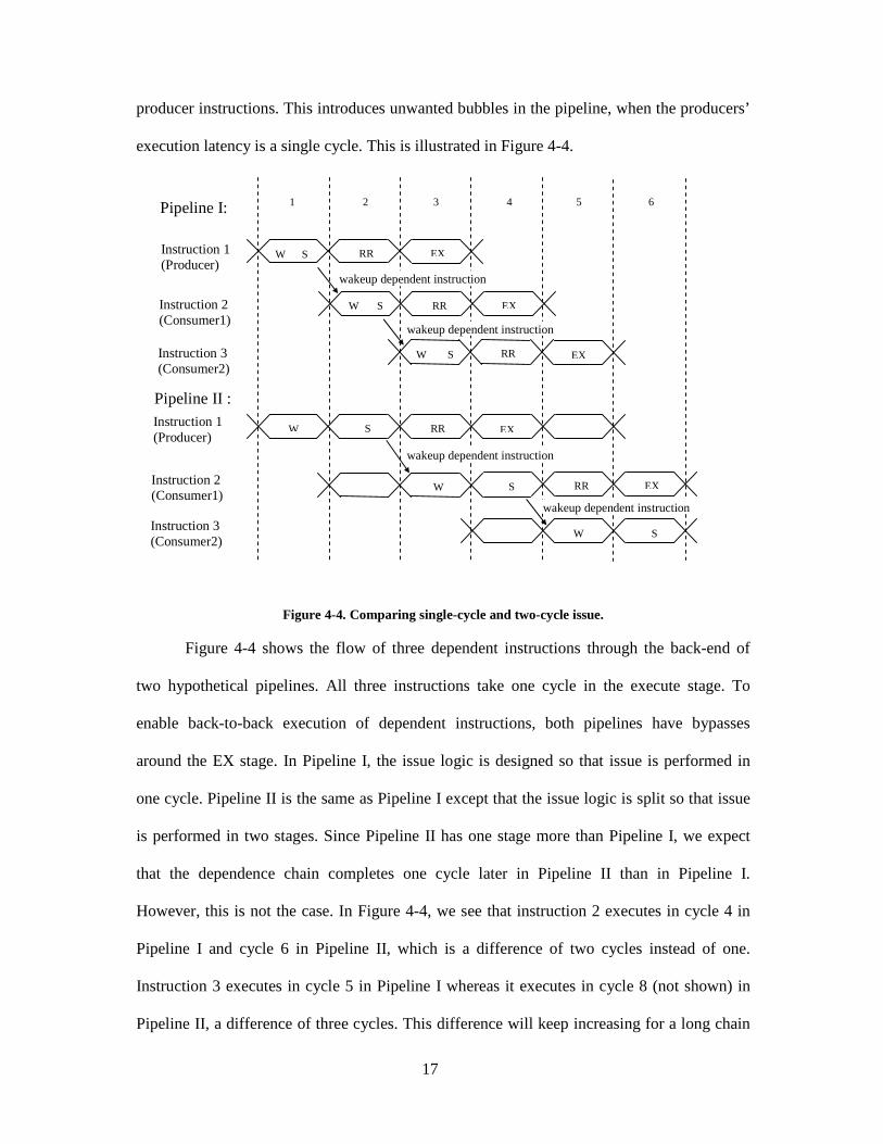
producer instructions. This introduces unwanted bubbles in the pipeline, when the producers’

execution latency is a single cycle. This is illustrated in Figure 4-4.

Figure 4-4. Comparing single-cycle and two-cycle issue.

Figure 4-4 shows the flow of three dependent instructions through the back-end of

two hypothetical pipelines. All three instructions take one cycle in the execute stage. To

enable back-to-back execution of dependent instructions, both pipelines have bypasses

around the EX stage. In Pipeline I, the issue logic is designed so that issue is performed in

one cycle. Pipeline II is the same as Pipeline I except that the issue logic is split so that issue

is performed in two stages. Since Pipeline II has one stage more than Pipeline I, we expect

that the dependence chain completes one cycle later in Pipeline II than in Pipeline I.

However, this is not the case. In Figure 4-4, we see that instruction 2 executes in cycle 4 in

Pipeline I and cycle 6 in Pipeline II, which is a difference of two cycles instead of one.

Instruction 3 executes in cycle 5 in Pipeline I whereas it executes in cycle 8 (not shown) in

Pipeline II, a difference of three cycles. This difference will keep increasing for a long chain

Pipeline II :Instruction 1(Producer)

Instruction 2(Consumer1)

Instruction 3(Consumer2)

Pipeline I:

Instruction 1(Producer)

Instruction 2(Consumer1)

Instruction 3(Consumer2)

W S

W

wakeup dependent instruction

W

S

W S

W S

W S

wakeup dependent instruction

wakeup dependent instruction

RR EX

S

wakeup dependent instruction

1 2 3 4 5 6

EX

EX

EX

EX

RR

RR

RR

RR

18

of dependent instructions, and degrading performance on Pipeline II. This happens because,

in Pipeline II, consumer instructions start their issue phase not one but two cycles after their

producer instructions do so.

To put it in more general terms, if the issue latency is greater than the execution

latency of the producer instruction, then unwanted bubbles are introduced in the pipeline.

Although the shortest execution latency in the deep pipeline is two cycles (simple

instructions), single-cycle latency can be effectively achieved using half-word bypassing.

This is discussed in the next section. To achieve back-to-back issue in deep mode, we

implement select-free issue logic [4].

Figure 4-5. Two-cycle issue with select-free scheduling [4].

Instructions can speculatively wake up dependent instructions by assuming that they

will issue as soon as they become ready [4]. Figure 4-5 shows the two-stage issue logic for a

deep pipeline, with select-free scheduling [4]. Each instruction in the issue queue has an entry

in the wakeup array called the dependence vector. A dependence vector contains information

about function unit requirements of each instruction. In addition, the vector also has one bit

for every instruction in the wakeup table. These bits indicate for a given instruction which

instructions in the wakeup array it depends on for its source operands. An instruction is ready

when all the source operands and function units it requires are available. The wakeup logic

determines this using the dependence vector information and constructs a request vector, i.e.,

DEP.VEC.

WAKEUPLOGIC

REQUEST

SCOREBOARD

GRANT REG.

READ

R

S

SELECTLOGIC

COLLISIONS

PILE UPS

SPECULATIVEWAKEUP

SHfree issuequeue entry

19

a one-hot vector denoting instructions that are ready to be executed. Once the request vector

is fed to the select logic, the scheduled (‘SH’) bits for all instructions in the request vector are

set speculatively, assuming that all instructions will be issued. This bit is used to trigger the

wakeup of dependent instructions.

The select logic chooses which of the ready instructions will issue. Arbitration is

required not only when the number of instructions is greater than the issue width, but also

when multiple instructions compete for the same function unit. The select logic determines

the instructions to be issued, usually based on age of the requesting instructions in the issue

queue, and generates a grant vector. Ready instructions that are not issued are considered to

have experienced a collision. These need to make another request to issue. This is done by

resetting the scheduled bit. Also, these instructions may have speculatively woken up their

consumer instructions. These wrongly woken-up instructions, referred to as pileups, are

detected by a scoreboard [4]. The scoreboard keeps track of all correctly issued instructions.

After a request to issue is granted to an instruction by the select logic, the scoreboard checks

if all its source registers are actually available (during the register read stage). If they are, the

instruction is considered to be correctly issued. Its destination registers are marked ready and

its entry in the wakeup array can be freed. If the source registers are not available, it implies

that the instruction has been wrongfully selected due to speculation. The instruction is

squashed and it needs to re-request to issue.

Collided and piled-up instructions have single-cycle latency before they can compete

again to be selected. This can be explained with an example. Consider that an instruction

requests to issue (i.e., wakes up) in cycle 1 and sets its scheduled bit speculatively. In cycle 2,

although the instruction has not been selected yet, it will not request to issue because its SH

bit is set. At the end of cycle 2, if this ready instruction is not selected, the instruction’s SH

bit is reset and it will be able to request again in cycle 3. If it collides again, the next request

20

will be made only in cycle 5, and so on. This latency to re-request is equal to the latency of

the select logic.

4.2.5 Execute stage

Simple instructions are the most commonly occurring instructions. Since these take

only one cycle to execute in shallow mode, back-to-back execution of simple instructions can

be enabled using conventional word bypasses. In deep mode, however, it takes two cycles to

execute a simple instruction. This may hinder back-to-back execution in the deep mode

because consumer instructions will start execution two cycles after their producers do so.

However, many ALU instructions can start their work even when only part of the

source data is available to them. For example, consider the add instruction in deep mode.

Figure 4-6 shows a circuit for a 2-stage adder. A[0:15], B[0:15], and SUM[0:15] are the

lower half-words of the two source operands and the result, respectively. A[16:31], B[16:31],

and SUM[16:31] are the upper half-words of the two source operands and result,

respectively. The add is performed over two cycles, EX1 and EX2. Consider two back-to-

back add instructions as follows.

AD1: ADD A1, B1, SUM1

AD2: ADD SUM1, B2, SUM2

The first two operands in the instruction denote the source operands and the third one

denotes the destination operand. We denote the first add instruction as AD1 and the second

add instruction as AD2. It can be observed that AD2 has a true dependency on AD1 (the first

source operand for AD2 is the same as the destination operand for AD1). Consider that AD1

begins its execution in cycle 1. In cycle 1, SUM1[0:15] is computed in the EX1 pipeline-

stage using A1[0:15] and B1[0:15]. Any carry generated as a result of this computation is

used along with A1[16:31] and B1[16:31] to compute SUM1[16:31] in the EX2 pipeline-

stage in cycle 2. In a conventional deep pipeline, AD2 would be able to begin execution only

21

Figure 4-6. Two-stage adder for deep mode.

Figure 4-7. Comparing half-word and full-word bypasses.

after AD1 is fully executed by the end of cycle 2. This causes a bubble in the pipeline, as

shown in CASE I in Figure 4-7. However, when AD2 is being processed in EX1, it only

requires the lower half-word of the result from AD1, i.e., SUM1[0:15]. SUM1[0:15] is

available as early as the beginning of cycle 2. Thus, AD2 can begin execution in cycle 2, if

EX1 EX2

A [16:31]

A [0:15]

B [16:31]

B [0:15]

SUM [16:31]

SUM [0:15]half-word bypass

half-word bypass

EX1

1

full-word bypass

2CASE I:

AD 1

43

CASE II:

EX2

EX2EX1AD 2

half-word bypasses

EX2

EX2

EX1

EX1AD 2

AD 1

22

the lower half-word of SUM1 is made available to it. In cycle 3, when AD1 has finished

execution, AD2 is in EX2 stage. It now uses the upper half-word of SUM1. Thus, back-to-

back execution of the two instructions is achieved using half-word bypassing. This is

depicted in CASE II of Figure 4-7. In shallow mode, however, since the ADD is performed in

a single cycle, half-word bypassing is not required. Thus, these bypasses need to be disabled

when the processor is operating in shallow mode. Figure 4-8 shows the circuit for the adder

in shallow mode. The half-word bypasses are disabled via the existing select signals to muxes

and the intermediate latches are made transparent, as shown in gray.

Figure 4-8. Single-stage adder for shallow mode.

PISA instruction type can produce low half-word early Can consume low half-word early

add, sub, bitwise-logical yes yes

left shift yes yes

right shift no yes

agen (part of load/store) yes(cache index) yes

load no agen: yes

store N/A agen: yes, data not needed until M2

slt no Yes

branch N/A Yes

lui produces full word at the end of RR2 N/A

float. pt. mul. div. , other no No

Table 4-1. PISA instructions that can produce/consume lower half-word early.

A [16:31]

B [16:31]

SUM [16:31]

EX

A [0:15]

B [0:15]

SUM [0:15]

23

Half-word bypassing is not feasible for all instructions. Table 4-1 shows which

instructions in Simplescalar’s PISA instruction set can produce a half-word at the end of the

EX1 stage and which instructions can begin executing as soon as the lower half-word is

available.

Half-word bypassing in the execute stage and select-free scheduling in the issue stage

go hand-in-hand. Instructions that produce their low half-word early also need to wake up

their dependent instructions speculatively, so that the half-word bypasses are exploited.

Instructions that do not produce their low half-word early do not wake up their dependent

instructions speculatively, since only the full-word bypasses can be used. The select-free

issue logic is modified accordingly so that instructions than can begin execution early (with

just the low half-word of a source operand) are woken up speculatively and instructions that

need the full word of the source operand are woken up non-speculatively. This is achieved by

having two bits for each instruction to record scheduling information instead of the single SH

Figure 4-9. Modified issue logic for deep mode.

bit as discussed earlier, i.e., a wakeup bit (W) and a selected bit (S). The modified design for

deep mode is shown in Figure 4-9.

An instruction sets its wakeup (W) bit when it is woken up and the selected (S) bit

when it is selected. The wakeup bit serves as a speculative wakeup flag and the selected bit

serves as a non-speculative wakeup flag. The dependence vector stores information regarding

DEP.VEC.

WAKEUPLOGIC

REQUEST

SCOREBOARD

GRANT

REG.READ

R

S

SELECTLOGIC

COLLISIONS

PILE UPS

W S

NON-SPECULATIVEWAKEUP

SPECULATIVEWAKEUP

S

R

free issuequeue entry

24

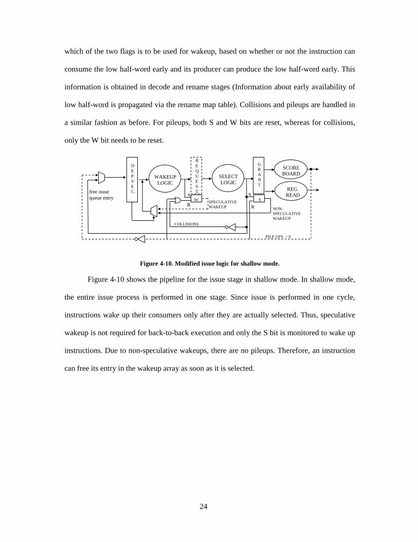
which of the two flags is to be used for wakeup, based on whether or not the instruction can

consume the low half-word early and its producer can produce the low half-word early. This

information is obtained in decode and rename stages (Information about early availability of

low half-word is propagated via the rename map table). Collisions and pileups are handled in

a similar fashion as before. For pileups, both S and W bits are reset, whereas for collisions,

only the W bit needs to be reset.

Figure 4-10. Modified issue logic for shallow mode.

Figure 4-10 shows the pipeline for the issue stage in shallow mode. In shallow mode,

the entire issue process is performed in one stage. Since issue is performed in one cycle,

instructions wake up their consumers only after they are actually selected. Thus, speculative

wakeup is not required for back-to-back execution and only the S bit is monitored to wake up

instructions. Due to non-speculative wakeups, there are no pileups. Therefore, an instruction

can free its entry in the wakeup array as soon as it is selected.

DEP.VEC.

WAKEUPLOGIC

REQUEST

SCOREBOARD

GRANT

REG.READ

R

S

SELECTLOGIC

COLLISIONS

PILE UPS = 0

W S

NON-SPECULATIVEWAKEUP

SPECULATIVEWAKEUP

S

R

free issuequeue entry

25

Chapter 5 Simulation Methodology

Independent experiments were performed using the two following simulators

1) An EDF scheduling simulator embedded with a frequency scaling algorithm.

2) A detailed cycle-accurate processor simulator. This simulator models the DPS-

enabled pipeline described in Chapter 4. Wattch power numbers and IPCs from

this simulator are used by the EDF scheduler.

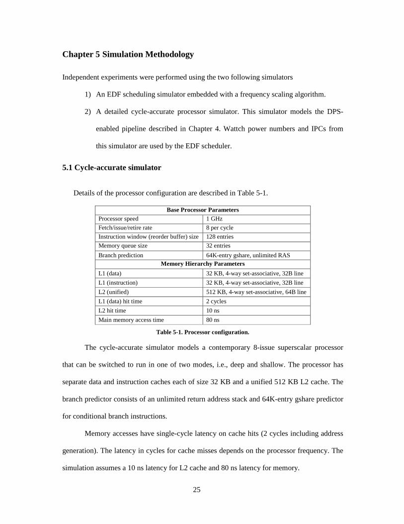
5.1 Cycle-accurate simulator

Details of the processor configuration are described in Table 5-1.

Base Processor ParametersProcessor speed 1 GHz

Fetch/issue/retire rate 8 per cycle

Instruction window (reorder buffer) size 128 entries

Memory queue size 32 entries

Branch prediction 64K-entry gshare, unlimited RASMemory Hierarchy Parameters

L1 (data) 32 KB, 4-way set-associative, 32B line

L1 (instruction) 32 KB, 4-way set-associative, 32B line

L2 (unified) 512 KB, 4-way set-associative, 64B line

L1 (data) hit time 2 cycles

L2 hit time 10 ns

Main memory access time 80 ns

Table 5-1. Processor configuration.

The cycle-accurate simulator models a contemporary 8-issue superscalar processor

that can be switched to run in one of two modes, i.e., deep and shallow. The processor has

separate data and instruction caches each of size 32 KB and a unified 512 KB L2 cache. The

branch predictor consists of an unlimited return address stack and 64K-entry gshare predictor

for conditional branch instructions.

Memory accesses have single-cycle latency on cache hits (2 cycles including address

generation). The latency in cycles for cache misses depends on the processor frequency. The

simulation assumes a 10 ns latency for L2 cache and 80 ns latency for memory.

26

5.2 Power modeling in cycle-accurate simulator

Wattch power models [3] were incorporated into the DPS-enabled processor simulator

to obtain cycle-accurate power information. The models estimate capacitance of various

structures based on their sizes and configuration. Dynamic power is then estimated using the

relation P =ÿ.C.V2.f. For simulations in this thesis clock gating was turned off.

The table below details the different voltage and frequency settings used in shallow

and deep modes in the processor simulator. These were derived from information available

for XScale microarchitecture [8].

Voltage f s fd

0.70 100 2000.82 200 4000.95 300 6001.07 400 8001.19 500 1000

Table 5-2. Voltage-frequency pairs for shallow and deep modes.

The simulator outputs accumulated power over all cycles for different frequencies.

This is averaged over all cycles (to obtain average power consumption) and fed to the EDF

scheduler simulator. Since frequency over a given time unit is constant, the scheduler

estimates energy consumed in one time unit to be Powerfreq, modex 1. Table 5-3 and Table 5-4

below show average power consumed when the processor is run at various voltage/frequency

levels in two different modes for the gap and bzip benchmarks, respectively.

Table 5-3. Power consumed in different modes on a variable-voltage processor, for the gap benchmark.

Voltage fshallow(MHz) Pshallow(W) fdeep(Mhz) Pdeep(W)

0.7 100 0.84 200 1.55

0.82 200 2.13 400 4.1

0.95 300 4.17 600 8.1

1.07 400 6.97 800 13.65

1.19 500 10.7 1000 21.25

27

Table 5-4. Power consumed in different modes on a variable-voltage processor, for the bzip benchmark.

On a variable-voltage processor, the power consumed at a given frequency in shallow

mode is more than the power consumed in deep mode because shallow mode requires a

higher operating voltage.

Table 5-5 shows the power consumed at different frequencies by a fixed-voltage

processor (V= 1.19 Volts, the peak voltage), for the gap and bzip benchmarks.

Frequency (Mhz) Gap: P (W) Bzip: P (W)

100 2.31 2.33

200 4.41 4.44

300 6.52 6.55

400 8.63 8.66

500 10.74 10.77

600 12.81 12.87

800 17.03 17.09

1000 21.25 21.31

Table 5-5. Power consumed on a fixed-voltage processor, for the gap and bzip benchmarks.

5.3 EDF scheduler simulator and frequency scaling algorithm

A frequency scaling algorithm was implemented by embedding it in a scheduling

simulator based on the Earliest-Deadline-First paradigm for periodic real-time tasks. A

prototype of this algorithm was developed for a course project. The prototype was improved

and modified to

• model scheduler invocation when a task completes before its allocated time slice,

• model the effect of voltage switching latency,

Voltage fshallow(MHz) Pshallow(W) fdeep(Mhz) Pdeep(W)

0.7 100 0.86 200 1.58

0.82 200 2.14 400 4.15

0.95 300 4.21 600 8.24

1.07 400 7.02 800 13.84

1.19 500 10.77 1000 21.31

28

• ensure safety in spite of multiple preemptions,

• model the effect of architectural variations due to pipeline switching on task

completion, and

• estimate energy consumption.

Frequency scaling is made possible by slack in the task schedule. This slack may be

either static slack or dynamic slack. Static slack is the slack existing in the schedule when all

tasks are assumed to take the worst-case execution time (WCET) and are run at peak

frequency. Dynamic slack is the slack accumulated dynamically when individual instances of

tasks take less time to execute than bounded by worst-case timing analysis.

Several algorithms have been proposed to scale frequency in order to optimize power

and energy consumption on variable-voltage processors. Most algorithms differ mainly in

their approaches for estimating and distributing the slack in the system among various tasks,

to run them at lower frequencies. However, none seem to have considered the latency

required to switch voltage. The electrical and thermal specifications manual for the Intel PXA

250 [7] specifies that voltage switching could have a maximum latency of 10 ms. The

minimum and typical values have not been specified. Pouwelse et al performed DVS on an

ARM processor and observed that when voltage was switched to a lower value, it took about

5.5 ms for the voltage to settle to the lower value [19]. This delay was attributed to the high

capacitance of the voltage regulator. These delays can be significant for fine-grained real-

time tasks with small deadlines.

The algorithm implemented for this thesis is a combination of the algorithms

developed by Srivastava et al [23] and Dudani et al. [2] along with a unique modification to

model the effect of voltage switching latency. At the beginning of the simulation, any static

slack existing in the task set is evenly distributed among all tasks by determining the

maximum constant frequency [23]. Because this is done prior to the execution of tasks, it

29

benefits voltage scaling, as switching penalties are not considered at this point. Dudani et al

propose to use slack with a greedy approach in which as much static slack as possible is

allocated to the current task at hand. However, a greedy approach is inefficient when the

voltage switching latency is high, because such an approach leads to more voltage

adjustments.

Dynamic slack generated by tasks is reclaimed as described by Dudani et al [2]. A

frequency decision is made on every task switch based on the available dynamic slack. Each

task’s execution time is split into two portions, the average execution time (Ca) and the

difference between worst-case and average execution times (Cb) [2]. The algorithm

speculates that the task will take only its typical execution time. However, reservations are

made to allow for a task to take its worst-case execution time and scaling is performed only

over the average portion of the execution time [2]. This can be expressed mathematically as

follows.

ba CCWCET +=

ba

ba

Cslack_usableCtime_Available

slack_usableCCtime_Available

slack_usableWCETtime_Available

++=

++=

+=

baba Cslack_usableCC

sf

C++=+

In the above equation, the scaling factor (sf) represents the ratio of the operating frequency to

the peak frequency of the processor.

At a given scheduling instant, the total slack existing in the system may be greater

than what can be utilized to scale frequency for the current task being scheduled. This is

because the dynamic slack generated by early completion of tasks having loose deadlines

cannot be passed to tasks that will be invoked in the future and have an earlier deadline. Also,

30

since voltage switching is not instantaneous, the scheduler considers each voltage switch as a

sporadic task that needs to be scheduled at that instant. To ensure safety, the scheduler checks

if there is enough slack between the current instant and deadline of the task being scheduled

at that instant.

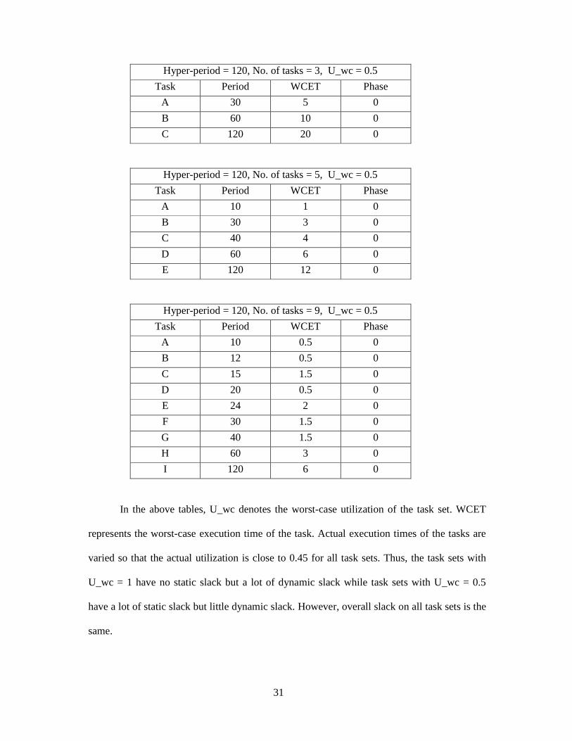
For our analysis, we are considering task sets with 3, 5, and 9 tasks. The hyper-period

for each of these task sets is 120 time units. Voltage switching latencies of 2 and 4 time units

were considered. When voltage scaling is disabled, frequency switching latency is taken to be

0.1 time units. The following task sets were used.

Hyper-period = 120, No. of tasks = 3, U_wc = 1

Task Period WCET Phase

A 30 10 0

B 60 20 0

C 120 40 0

Hyper-period = 120, No. of tasks = 5, U_wc = 1

Task Period WCET Phase

A 10 2 0

B 30 6 0

C 40 8 0

D 60 12 0

E 120 24 0

Hyper-period = 120, No. of tasks = 9, U_wc = 1

Task Period WCET Phase

A 10 1 0

B 12 1 0

C 15 3 0

D 20 1 0

E 24 4 0

F 30 3 0

G 40 1 0

H 60 6 0

I 120 12 0

31

Hyper-period = 120, No. of tasks = 3, U_wc = 0.5

Task Period WCET Phase

A 30 5 0

B 60 10 0

C 120 20 0

Hyper-period = 120, No. of tasks = 5, U_wc = 0.5

Task Period WCET Phase

A 10 1 0

B 30 3 0

C 40 4 0

D 60 6 0

E 120 12 0

Hyper-period = 120, No. of tasks = 9, U_wc = 0.5

Task Period WCET Phase

A 10 0.5 0

B 12 0.5 0

C 15 1.5 0

D 20 0.5 0

E 24 2 0

F 30 1.5 0

G 40 1.5 0

H 60 3 0

I 120 6 0

In the above tables, U_wc denotes the worst-case utilization of the task set. WCET

represents the worst-case execution time of the task. Actual execution times of the tasks are

varied so that the actual utilization is close to 0.45 for all task sets. Thus, the task sets with

U_wc = 1 have no static slack but a lot of dynamic slack while task sets with U_wc = 0.5

have a lot of static slack but little dynamic slack. However, overall slack on all task sets is the

same.

32

Chapter 6 Results

6.1 Experiments with the cycle-accurate processor simulator

We ran ten Spec2K benchmarks on the detailed cycle-accurate processor simulator

(described in the previous chapter) for 25 million instructions after having skipped the first 1

billion instructions.

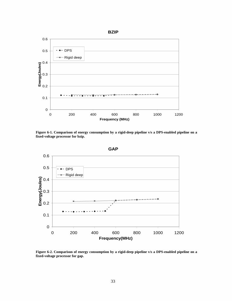
6.1.1 Comparison of energy consumption on a fixed-voltage processor

Figures 6-1 through 6-10 compare the energy consumed by a rigid deep pipeline and

the energy consumed by a DPS-enabled pipeline, on a fixed-voltage processor. It can be seen

that the energy savings with a DPS-enabled pipeline ranges from 6.5% for bzip to 40% for

gap. Other benchmarks have energy savings between 21%-29%. Bzip has a near-100%

branch prediction accuracy and cache hit rates. The L1 data and instruction cache miss rates

for bzip are about 0.2% and 0%, respectively. The two primary causes for differences in

energy between the shallow and deep pipelines -- branch misprediction penalties and data

stalls -- are minimal for bzip. This is the cause for low energy savings with bzip. It can also

be seen that on a fixed-voltage processor, energy consumption is fairly constant with

variations in frequency, for most benchmarks. Mcf is an anomalous case here. There is a 2.6x

variation in energy with a 5x variation in frequency. This is because mcf is a memory

intensive benchmark. As frequency is lowered, the memory latency in terms of cycles is also

reduced. This results in fewer data stall cycles at lower frequencies. Since clock gating is

disabled, reducing the frequency results in lower energy for mcf.

33

BZIP

0

0.1

0.2

0.3

0.4

0.5

0.6

0 200 400 600 800 1000 1200Frequency (MHz)

Ene

rgy(

Joul

es)

DPS

Rigid deep

Figure 6-1. Comparison of energy consumption by a rigid-deep pipeline v/s a DPS-enabled pipeline on afixed-voltage processor for bzip.

GAP

0

0.1

0.2

0.3

0.4

0.5

0.6

0 200 400 600 800 1000 1200Frequency(MHz)

Ene

rgy(

Joul

es)

DPS

Rigid deep

Figure 6-2. Comparison of energy consumption by a rigid-deep pipeline v/s a DPS-enabled pipeline on afixed-voltage processor for gap.

34

GCC

0

0.1

0.2

0.3

0.4

0.5

0.6

0 200 400 600 800 1000 1200Frequency(MHz)

Ene

rgy(

Joul

es)

DPS

Rigid deep

Figure 6-3. Comparison of energy consumption by a rigid-deep pipeline v/s a DPS-enabled pipeline on afixed-voltage processor for gcc.

GZIP

0

0.1

0.2

0.3

0.4

0.5

0.6

0 200 400 600 800 1000 1200Frequency(MHz)

Ene

rgy(

Joul

es)

DPS

Rigid deep

Figure 6-4. Comparison of energy consumption by a rigid-deep pipeline v/s a DPS-enabled pipeline on afixed-voltage processor for gzip.

35

MCF

0

0.2

0.4

0.6

0.8

1

1.2

1.4

1.6

1.8

2

0 200 400 600 800 1000 1200Frequency(MHz)

Ene

rgy(

Joul

es)

DPS

Rigid deep

Figure 6-5. Comparison of energy consumption by a rigid-deep pipeline v/s a DPS-enabled pipeline on afixed-voltage processor for mcf.

PARSER

0

0.1

0.2

0.3

0.4

0.5

0.6

0 200 400 600 800 1000 1200Frequency(MHz)

Ene

rgy(

Joul

es)

DPS

Rigid deep

Figure 6-6. Comparison of energy consumption by a rigid-deep pipeline v/s a DPS-enabled pipeline on afixed-voltage processor for parser.

36

PERL

0

0.1

0.2

0.3

0.4

0.5

0.6

0 200 400 600 800 1000 1200Frequency(MHz)

Ene

rgy(

Joul

es)

DPS

Rigid deep

Figure 6-7. Comparison of energy consumption by a rigid-deep pipeline v/s a DPS-enabled pipeline on afixed-voltage processor for perl.

TWOLF

0

0.2

0.4

0.6

0.8

1

0 200 400 600 800 1000 1200Frequency(MHz)

Ene

rgy(

Joul

es)

DPS

Rigid deep

Figure 6-8. Comparison of energy consumption by a rigid-deep pipeline v/s a DPS-enabled pipeline on afixed-voltage processor for twolf.

37

VORTEX

0

0.1

0.2

0.3

0.4

0.5

0.6

0 200 400 600 800 1000 1200Frequency(MHz)

Ene

rgy(

Joul

es)

DPS

Rigid deep

Figure 6-9. Comparison of energy consumption by a rigid-deep pipeline v/s a DPS-enabled pipeline on afixed-voltage processor for vortex.

VPR

0

0.1

0.2

0.3

0.4

0.5

0.6

0 200 400 600 800 1000 1200Frequency(MHz)

Ene

rgy(

Joul

es)

DPS

Rigid deep

Figure 6-10. Comparison of energy consumption by a rigid-deep pipeline v/s a DPS-enabled pipeline on afixed-voltage processor for vpr.

38

Figure 6-11 shows the percentage energy savings of a DPS-enabled pipeline over a

rigid-deep pipeline for the gcc benchmark at 200 MHz, for a fixed-voltage processor with

four modes. These modes are described below.

I: Real branch prediction, no clock gating.

II: Perfect branch prediction, no clock gating.

III: Real branch prediction, perfect clock gating.

IV: Perfect branch prediction, perfect clock gating.

Perfect clock gating eliminates the energy wasted due to data stall cycles. With perfect

branch prediction, there are no instructions executed down the wrong path. Thus, the energy

wasted due to wrong-path instructions is eliminated with perfect branch prediction. It can be

inferred from the graph below that the energy benefits due to DPS are minimal when the

processor operates in mode IV. This confirms our hypothesis that shallow pipelines are more

energy-efficient due to fewer wasteful transitions.

Figure 6-11 shows that in spite of perfect branch prediction and perfect clock gating

there is some residual energy savings with a DPS-enabled pipeline. This is due to the energy

wasted by collisions and pileups that are generated by the two-stage issue logic in deep mode.

Figure 6-11. Confirmation that energy difference between shallow and deep modes is due to wastefultransitions.

% Energy savings of a DPS-enabled pipelineover a rigid-deep pipeline for gcc at 200 MHz

0

5

10

15

20

25

30

I II III IV

%E

nerg

yS

avin

gs

39

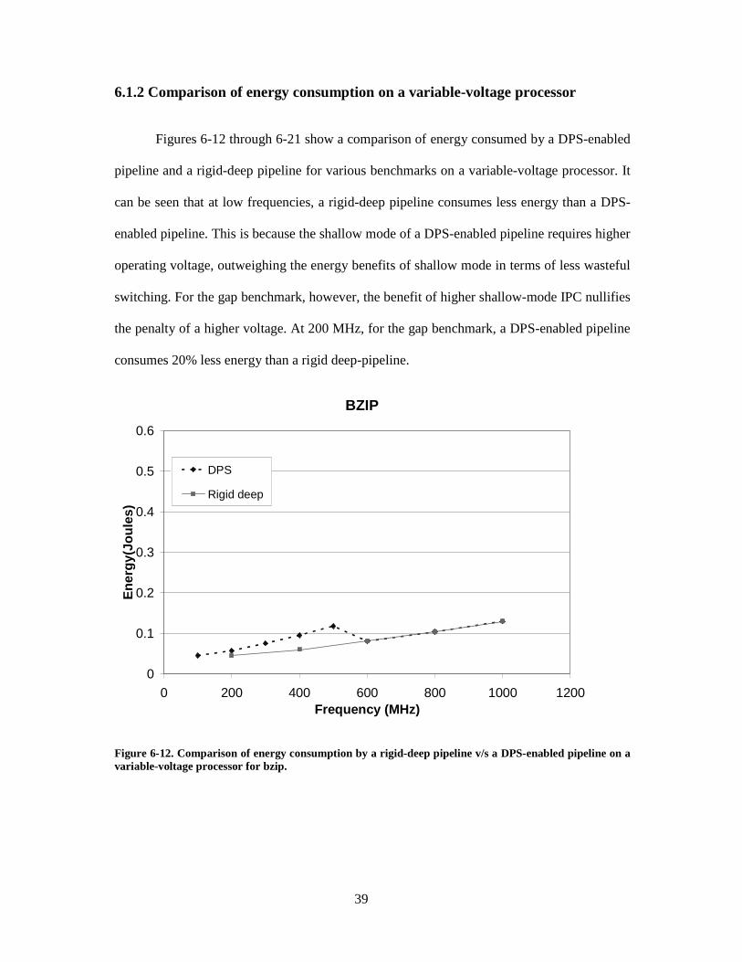
6.1.2 Comparison of energy consumption on a variable-voltage processor

Figures 6-12 through 6-21 show a comparison of energy consumed by a DPS-enabled

pipeline and a rigid-deep pipeline for various benchmarks on a variable-voltage processor. It

can be seen that at low frequencies, a rigid-deep pipeline consumes less energy than a DPS-

enabled pipeline. This is because the shallow mode of a DPS-enabled pipeline requires higher

operating voltage, outweighing the energy benefits of shallow mode in terms of less wasteful

switching. For the gap benchmark, however, the benefit of higher shallow-mode IPC nullifies

the penalty of a higher voltage. At 200 MHz, for the gap benchmark, a DPS-enabled pipeline

consumes 20% less energy than a rigid deep-pipeline.

BZIP

0

0.1

0.2

0.3

0.4

0.5

0.6

0 200 400 600 800 1000 1200Frequency (MHz)

Ene

rgy(

Joul

es)

DPS

Rigid deep

Figure 6-12. Comparison of energy consumption by a rigid-deep pipeline v/s a DPS-enabled pipeline on avariable-voltage processor for bzip.

40

GAP

0

0.1

0.2

0.3

0.4

0.5

0.6

0 200 400 600 800 1000 1200Frequency(MHz)

Ene

rgy(

Joul

es)

DPS

Rigid deep

Figure 6-13. Comparison of energy consumption by a rigid-deep pipeline v/s a DPS-enabled pipeline on avariable-voltage processor for gap.

GCC

0

0.1

0.2

0.3

0.4

0.5

0.6

0.7

0.8

0.9

1

0 200 400 600 800 1000 1200Frequency(MHz)

Ene

rgy(

Joul

es)

DPS

Rigid deep

Figure 6-14. Comparison of energy consumption by a rigid-deep pipeline v/s a DPS-enabled pipeline on avariable-voltage processor for gcc.

41

GZIP

0

0.1

0.2

0.3

0.4

0.5

0.6

0 200 400 600 800 1000 1200Frequency(MHz)

Ene

rgy(

Joul

es)

DPS

Rigid deep

Figure 6-15. Comparison of energy consumption by a rigid-deep pipeline v/s a DPS-enabled pipeline on avariable-voltage processor for gzip.

MCF

0

0.2

0.4

0.6

0.8

1

1.2

1.4

1.6

1.8

2

0 200 400 600 800 1000 1200Frequency(MHz)

Ene

rgy(

Joul

es)

DPS

Rigid deep

Figure 6-16. Comparison of energy consumption by a rigid-deep pipeline v/s a DPS-enabled pipeline on avariable-voltage processor for mcf.

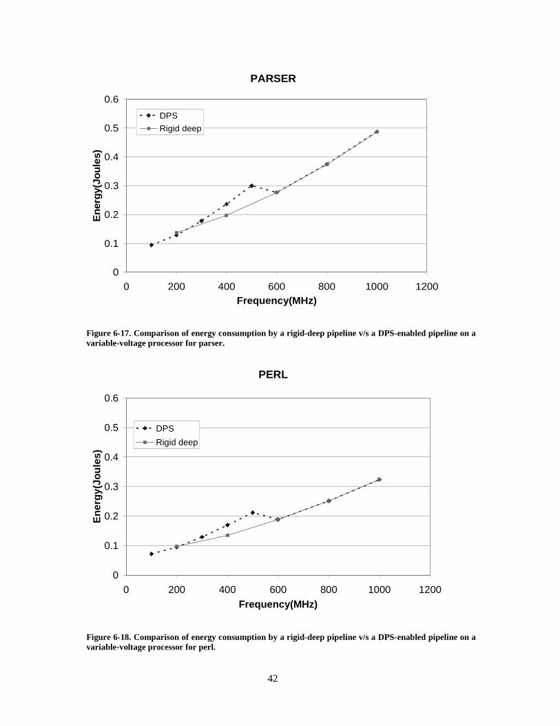
42

PARSER

0

0.1

0.2

0.3

0.4

0.5

0.6

0 200 400 600 800 1000 1200Frequency(MHz)

Ene

rgy(

Joul

es)

DPS

Rigid deep

Figure 6-17. Comparison of energy consumption by a rigid-deep pipeline v/s a DPS-enabled pipeline on avariable-voltage processor for parser.

PERL

0

0.1

0.2

0.3

0.4

0.5

0.6

0 200 400 600 800 1000 1200Frequency(MHz)

Ene

rgy(

Joul

es)

DPS

Rigid deep

Figure 6-18. Comparison of energy consumption by a rigid-deep pipeline v/s a DPS-enabled pipeline on avariable-voltage processor for perl.

43

TWOLF

0

0.1

0.2

0.3

0.4

0.5

0.6

0.7

0.8

0.9

1

0 200 400 600 800 1000 1200Frequency(MHz)

Ene

rgy(

Joul

es)

DPS

Rigid deep

Figure 6-19. Comparison of energy consumption by a rigid-deep pipeline v/s a DPS-enabled pipeline on avariable-voltage processor for twolf.

VORTEX

0

0.1

0.2

0.3

0.4

0.5

0.6

0 200 400 600 800 1000 1200Frequency(MHz)

Ene

rgy(

Joul

es)

DPS

Rigid deep

Figure 6-20. Comparison of energy consumption by a rigid-deep pipeline v/s a DPS-enabled pipeline on avariable-voltage processor for vortex.

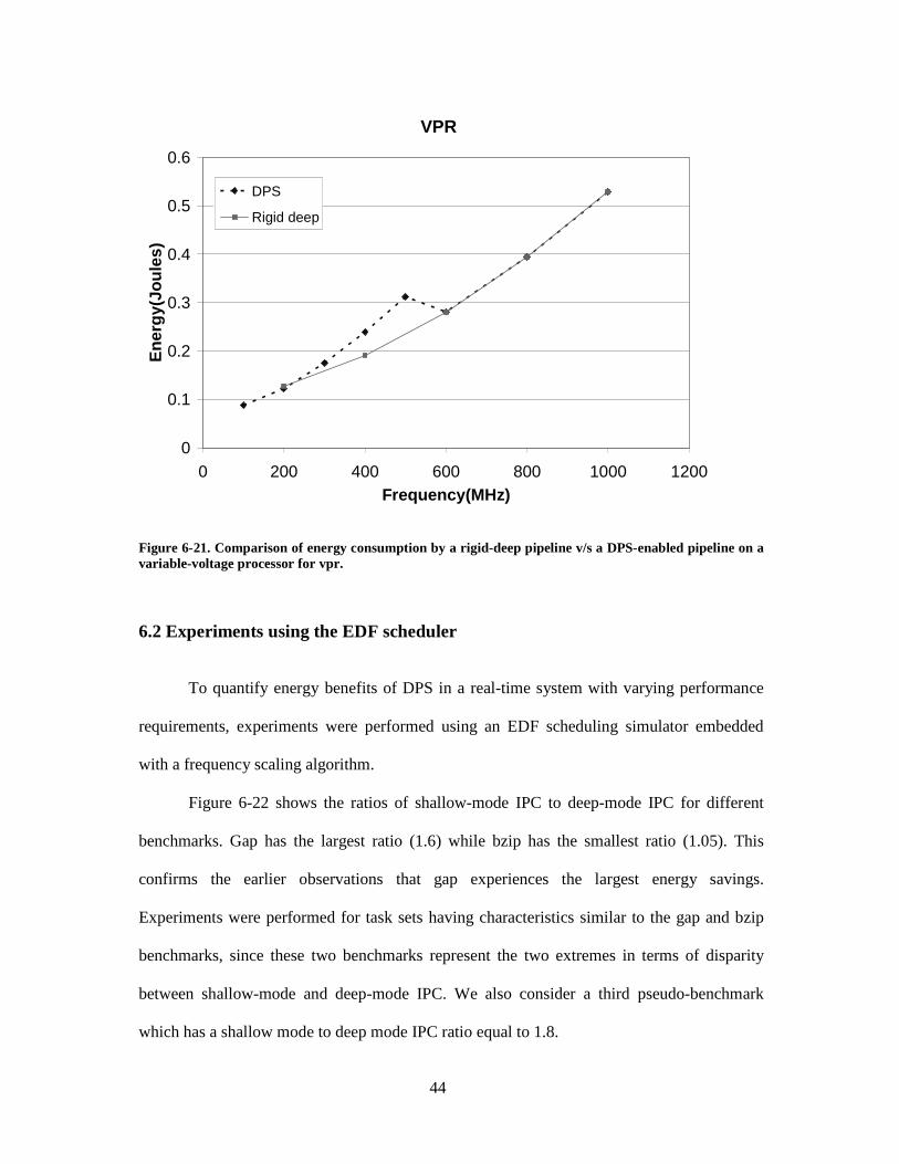
44

VPR

0

0.1

0.2

0.3

0.4

0.5

0.6

0 200 400 600 800 1000 1200Frequency(MHz)

Ene

rgy(

Joul

es)

DPS

Rigid deep

Figure 6-21. Comparison of energy consumption by a rigid-deep pipeline v/s a DPS-enabled pipeline on avariable-voltage processor for vpr.

6.2 Experiments using the EDF scheduler

To quantify energy benefits of DPS in a real-time system with varying performance

requirements, experiments were performed using an EDF scheduling simulator embedded

with a frequency scaling algorithm.

Figure 6-22 shows the ratios of shallow-mode IPC to deep-mode IPC for different

benchmarks. Gap has the largest ratio (1.6) while bzip has the smallest ratio (1.05). This

confirms the earlier observations that gap experiences the largest energy savings.

Experiments were performed for task sets having characteristics similar to the gap and bzip

benchmarks, since these two benchmarks represent the two extremes in terms of disparity

between shallow-mode and deep-mode IPC. We also consider a third pseudo-benchmark

which has a shallow mode to deep mode IPC ratio equal to 1.8.

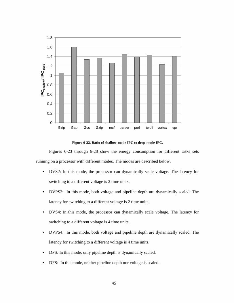
45

0

0.2

0.4

0.6

0.8

1

1.2

1.4

1.6

1.8

Bzip Gap Gcc Gzip mcf parser perl twolf vortex vpr

IPC

shal

low

/IP

Cde

ep

Figure 6-22. Ratio of shallow-mode IPC to deep-mode IPC.

Figures 6-23 through 6-28 show the energy consumption for different tasks sets

running on a processor with different modes. The modes are described below.

• DVS2: In this mode, the processor can dynamically scale voltage. The latency for

switching to a different voltage is 2 time units.

• DVPS2: In this mode, both voltage and pipeline depth are dynamically scaled. The

latency for switching to a different voltage is 2 time units.

• DVS4: In this mode, the processor can dynamically scale voltage. The latency for

switching to a different voltage is 4 time units.

• DVPS4: In this mode, both voltage and pipeline depth are dynamically scaled. The

latency for switching to a different voltage is 4 time units.

• DPS: In this mode, only pipeline depth is dynamically scaled.

• DFS: In this mode, neither pipeline depth nor voltage is scaled.

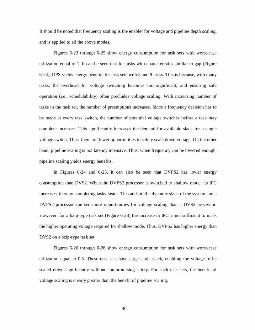
46

It should be noted that frequency scaling is the enabler for voltage and pipeline depth scaling,

and is applied to all the above modes.

Figures 6-23 through 6-25 show energy consumption for task sets with worst-case

utilization equal to 1. It can be seen that for tasks with characteristics similar to gap (Figure

6-24), DPS yields energy benefits for task sets with 5 and 9 tasks. This is because, with many

tasks, the overhead for voltage switching becomes too significant, and ensuring safe

operation (i.e., schedulability) often precludes voltage scaling. With increasing number of

tasks in the task set, the number of preemptions increases. Since a frequency decision has to

be made at every task switch, the number of potential voltage switches before a task may

complete increases. This significantly increases the demand for available slack for a single

voltage switch. Thus, there are fewer opportunities to safely scale down voltage. On the other

hand, pipeline scaling is not latency intensive. Thus, when frequency can be lowered enough,

pipeline scaling yields energy benefits.

In Figures 6-24 and 6-25, it can also be seen that DVPS2 has lower energy

consumption than DVS2. When the DVPS2 processor is switched to shallow mode, its IPC

increases, thereby completing tasks faster. This adds to the dynamic slack of the system and a

DVPS2 processor can see more opportunities for voltage scaling than a DVS2 processor.

However, for a bzip-type task set (Figure 6-23) the increase in IPC is not sufficient to mask

the higher operating voltage required for shallow mode. Thus, DVPS2 has higher energy than

DVS2 on a bzip-type task set.

Figures 6-26 through 6-28 show energy consumption for task sets with worst-case

utilization equal to 0.5. These task sets have large static slack, enabling the voltage to be

scaled down significantly without compromising safety. For such task sets, the benefit of

voltage scaling is clearly greater than the benefit of pipeline scaling.

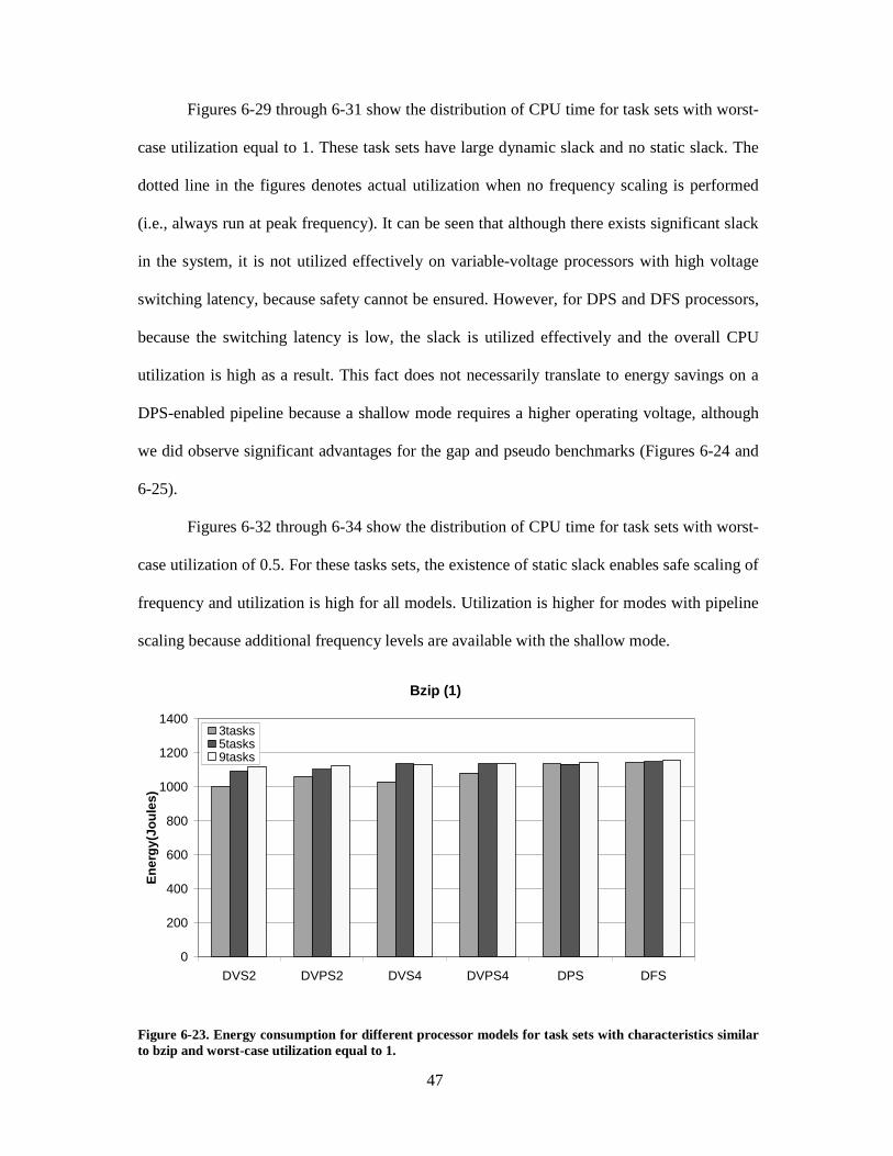
47

Figures 6-29 through 6-31 show the distribution of CPU time for task sets with worst-

case utilization equal to 1. These task sets have large dynamic slack and no static slack. The

dotted line in the figures denotes actual utilization when no frequency scaling is performed

(i.e., always run at peak frequency). It can be seen that although there exists significant slack

in the system, it is not utilized effectively on variable-voltage processors with high voltage

switching latency, because safety cannot be ensured. However, for DPS and DFS processors,

because the switching latency is low, the slack is utilized effectively and the overall CPU

utilization is high as a result. This fact does not necessarily translate to energy savings on a

DPS-enabled pipeline because a shallow mode requires a higher operating voltage, although

we did observe significant advantages for the gap and pseudo benchmarks (Figures 6-24 and

6-25).

Figures 6-32 through 6-34 show the distribution of CPU time for task sets with worst-

case utilization of 0.5. For these tasks sets, the existence of static slack enables safe scaling of

frequency and utilization is high for all models. Utilization is higher for modes with pipeline

scaling because additional frequency levels are available with the shallow mode.

Bzip (1)

0

200

400

600

800

1000

1200

1400

DVS2 DVPS2 DVS4 DVPS4 DPS DFS

Ene

rgy(

Joul

es)

3tasks5tasks9tasks

Figure 6-23. Energy consumption for different processor models for task sets with characteristics similarto bzip and worst-case utilization equal to 1.

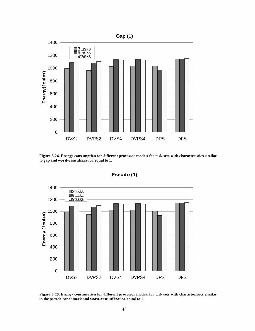
48

Gap (1)

0

200

400

600

800

1000

1200

1400

DVS2 DVPS2 DVS4 DVPS4 DPS DFS

Ene

rgy(

Joul

es)

3tasks5tasks9tasks

Figure 6-24. Energy consumption for different processor models for task sets with characteristics similarto gap and worst-case utilization equal to 1.

Pseudo (1)

0

200

400

600

800

1000

1200

1400

DVS2 DVPS2 DVS4 DVPS4 DPS DFS

Ene

rgy

(Jou

les)

3tasks5tasks9tasks

Figure 6-25. Energy consumption for different processor models for task sets with characteristics similarto the pseudo benchmark and worst-case utilization equal to 1.

49

Bzip (0.5)

0

200

400

600

800

1000

1200

1400

DVS2 DVPS2 DVS4 DVPS4 DPS DFS

Ene

rgy(

Joul

es)

3tasks5tasks9tasks

Figure 6-26. Energy consumption for different processor models for task sets with characteristics similarto bzip and worst-case utilization equal to 0.5.

Gap (0.5)

0

200

400

600

800

1000

1200

1400

DVS2 DVPS2 DVS4 DVPS4 DPS DFS

Ene

rgy(

Joul

es)

3tasks5tasks9tasks

Figure 6-27. Energy consumption for different processor models for task sets with characteristics similarto gap and worst-case utilization equal to 0.5.

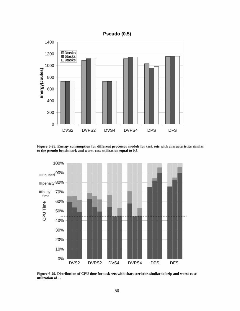
50

Pseudo (0.5)

0

200

400

600

800

1000

1200

1400

DVS2 DVPS2 DVS4 DVPS4 DPS DFS

Ene

rgy(

Joul

es)

3tasks5tasks9tasks

Figure 6-28. Energy consumption for different processor models for task sets with characteristics similarto the pseudo benchmark and worst-case utilization equal to 0.5.

0%

10%

20%

30%

40%

50%

60%

70%

80%

90%

100%

1

CP

UT

ime

unused

penalty

busytime

DVS2 DVPS2 DVPS4 DPS DFSDVS4

Figure 6-29. Distribution of CPU time for task sets with characteristics similar to bzip and worst-caseutilization of 1.

51

0%

10%

20%

30%

40%

50%

60%

70%

80%

90%

100%

1

CP

UT

ime

unused

penalty

busytime

DVS2 DVPS2 DVPS4 DPS DFSDVS4

Figure 6-30. Distribution of CPU time for task sets with characteristics similar to gap and worst-caseutilization of 1.

0%

10%

20%

30%

40%

50%

60%

70%

80%

90%

100%

1

CP

UT

ime

unused

penalty

busytime

DVS2 DVPS2 DVPS4 DPS DFSDVS4

Figure 6-31. Distribution of CPU time for task sets with characteristics similar to the pseudo benchmarkand worst-case utilization of 1.

52

0%

10%

20%

30%

40%

50%

60%

70%

80%

90%

100%

1

CP

UT

ime

unused

penalty

busytime

DVS2 DVPS2 DVPS4 DPS DFSDVS4

Figure 6-32. Distribution of CPU time for task sets with characteristics similar to bzip and worst-caseutilization of 0.5.

0%

10%

20%

30%

40%

50%

60%

70%

80%

90%

100%

1

CP

UT

ime

unused

penalty

busytime

DVS2 DVPS2 DVPS4 DPS DFSDVS4

Figure 6-33. Distribution of CPU time for task sets with characteristics similar to gap and worst-caseutilization of 0.5.

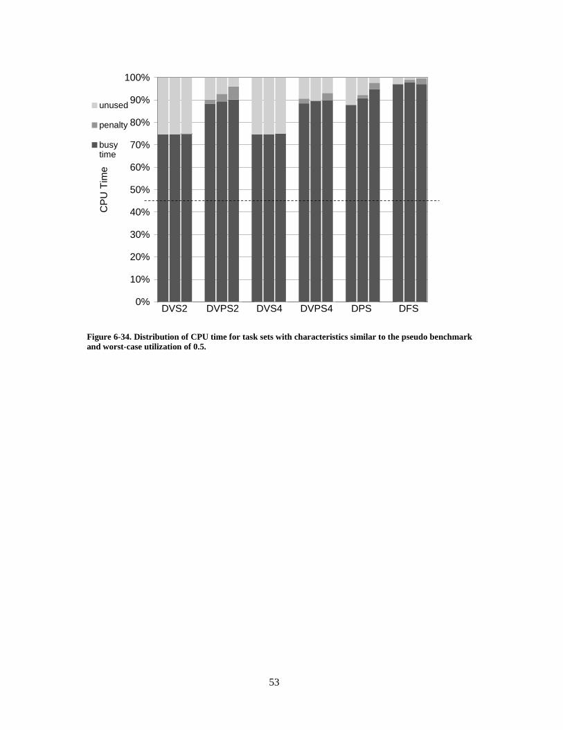
53

0%

10%

20%

30%

40%

50%

60%

70%

80%

90%

100%

1

CP

UT

ime

unused

penalty

busytime

DVS2 DVPS2 DVPS4 DPS DFSDVS4

Figure 6-34. Distribution of CPU time for task sets with characteristics similar to the pseudo benchmarkand worst-case utilization of 0.5.

54

Chapter 7 Summary and Future Work

When voltage scaling is not desirable or achievable, frequency scaling can still yield

energy benefits. Dynamic pipeline scaling (DPS) provides a microarchitectural substrate for

achieving this. When frequency is lowered enough, adjacent pipeline stages can be merged to

obtain a shallow pipeline that is half as deep. The shallow pipeline is more energy-efficient

than the deep pipeline, when they both operate at equal voltage and frequency. This is

because the shallow pipeline has fewer data stalls and lower branch misprediction penalties.

The minimum branch misprediction penalty for the shallow pipeline is half that of the deep

pipeline. Having fewer data stall cycles implies less useless switching and having lower

branch misprediction penalties implies fewer instructions fetched and executed down the

wrong path. These factors combine to make a shallow pipeline more energy-efficient.

Experiments using a detailed cycle-accurate processor simulator showed that a DPS-

enabled pipeline consumes from 6.5% to 40% less energy than a rigid-deep pipeline, on a

fixed-voltage processor. For a real-time system with many fine-grained tasks on a variable-

voltage processor, a DPS-enabled pipeline can be more energy-efficient than a rigid-deep

pipeline, depending on the nature of the tasks.

Future work includes a detailed analysis of the limitations of voltage scaling,

including future technology trends. An interesting project would be to implement dynamic

pipeline scaling on an existing verilog model of a processor and study the benefits. A high

priority future study is to compare a DPS-enabled pipeline to a pipeline with fetch-gating and

clock-gating support. Isolating dynamic pipeline scaling to regions in the program with long

dependence chains or badly behaving branches could accentuate the benefits of pipeline

scaling on a variable-voltage processor. Application of pipeline scaling to fully wave-

pipelined circuits would be an interesting study.

55

References

[1] D. H. Albonesi. Selective Cache Ways: On-Demand Cache Resource Allocation.32nd Int’l Symp. on

Microarchitecture,November 1999.

[2] A. Dudani, F. Mueller, Y. Zhu. Energy-Conserving Feedback EDF Scheduling for Embedded Systems with

Real-Time Constraints.Languages, Compilers, and Tools for Embedded Systems (LCTES),June 2002.

[3] D. Brooks, V. Tiwari, and M. Martonosi. Wattch: A Framework for Architectural-Level Power Analysis

and Optimizations. 27th Int’l Symp. on Computer Architecture,June 2000.

[4] M. D. Brown, J. Stark, and Y. N. Patt. Select-Free Instruction Scheduling Logic.34th Int’l Symp. on

Microarchitecture,December 2001.

[5] T. D. Burd and R. W. Brodersen. Energy Efficient CMOS Microprocessor Design.Kluwer Academic

Publishers, 2002.

[6] D. Burger, T. M. Austin, and S. Bennet. Evaluating Future Microprocessors: The Simplescalar Tool Set.

Tech. Rep.CS-TR-96-1308, University Of Wisconsin, Madison, July 1996.

[7] Intel® PXA250 and PXA210 Applications Processors Electrical, Mechanical, and Thermal Specifications.

[ftp://download.intel.com/design/pca/applicationsprocessors/manuals/278524-001.pdf]

[8] Intel XScale Microarchitecture.

[http://www.intel.com/design/intelxscale/benchmarks.htm]

[9] K. Govil, E Chan, and H. Wasserman. Comparing Algorithms for Dynamic Speed-Setting of a Low-Power

CPU.1st Int’l Conf. on Mobile Computing and Networking,November 1995.

[10] D. Grunwald, P. Levis, C Morrey III, M. Neufeld, and K. Farkas. Policies for Dynamic Clock Scheduling.

Symposium on Operating Systems Design and Implementation, October 2000.

[11] J. L. Hennessy and D. A. Patterson. Computer Architecture: A Quantitative Approach.Morgan Kauffman

Publishers.Second Edition. 1995.

[12] I. Hong, M. Potkonjak, and M. Srivastava. On-line Scheduling of Hard Real-Time Tasks on Variable

Voltage Processors.Int’l Conf. on Computer-Aided Design, November 1998.

56

[13] D.A. Jimenez. Reconsidering Complex Branch Predictors.9th Int’l Symp. on High Performance Computer

Architecture,February 2003.

[14] J. Koppanalil, P. Ramrakhyani, S. Desai, A. Vaidyanathan, and E. Rotenberg. A Case for Dynamic Pipeline

Scaling. International Conference on Compilers, Architecture, and Synthesis for Embedded Systems,

October 2002.

[15] Y. Lee and C. Krishna. Voltage Clock Scaling for Low Energy Consumption in Real-Time Embedded

Systems.6th Int’l Conf. on Real-Time Computing Systems and Applications,December 1999.

[16] J. Lorch and A. J. Smith. Improving Dynamic Voltage Scaling Algorithms with PACE.ACM SIGMETRICS

2001 Conf.,June 2001.

[17] S. Manne, A. Klauser, and D. Grunwald. Pipeline Gating: Speculation Control for Energy Reduction.25th

Int’l Symp. on Computer Architecture, June 1998.

[18] K. Olukotun, T. Mudge, and R. Brown. Performance Optimization of Pipelined Caches.19th Annual

International Symposium on Computer Architecture,June 1992.

[19] J. Pouwelse, K. Langendoen, and H. Sips. Dynamic voltage scaling on a low-power microprocessor.

Seventh ACM Annual International Conference on Mobile Computing and Networking,2001.

[20] R. Secareanu, D. Albonesi, and E. Friedman. A Dynamic Reconfigurable Clock Generator.IEEE ASIC

Conference, September 2001.

[21] A. Seznec, P. Sainrat, and P.Michaud. Multiple-Block Ahead Branch Predictors. 7th Int’l Conf.on Arch.

Support for Prog. Lang. and Operating Systems,October 1996.

[22] A. Srivastava, Y. Koh, B. Sano and A. Despain. 190-MHz CMOS 4-Kbyte Pipelined Caches.Int’l

Symposium on Circuits and SystemsApril 1995.

[23] Y Shin, K. Choi, and T. Sakurai. Power Optimization of Real Time Embedded Systems on Variable Speed

Processors.Int’l Conference on Computer-Aided Design,November 2000.

[24] T. Pering, T. Burd, and R. Brodersen. The Simulation of dynamic Voltage Scaling Algorithms.Symposium

on Low Power Electronics,October 2000.

[25] M. Weiser, B. Welch, A. Demers, and S. Shenker. Scheduling for Reduced CPU Energy.1st Symp. on

Operating Systems Design and Implementation,November 1994.

57

[26] Alpha 21264 Microprocessor Hardware Reference Manual.

[http://ftp.digital.com/pub/Digital/info/semiconductor/literature/21264hrm.pdf]