Random Assignmentson Sequentially Dichotomous Domains ∗

Peng Liu†

September 17, 2018

Abstract

We present a possibility result on the existence of a random assignment rule satisfy-ing sd-strategy-proofness, sd-efficiency, and equal treatment of equals. In particular, weintroduce a class of preference domains: sequentially dichotomous domains. On any suchdomain, the probabilistic serial rule (Bogomolnaia and Moulin (2001)) is sd-strategy-proof.Moreover, any sequentially dichotomous domain is maximal for this rule to be sd-strategy-proof.

Keywords: Random assignment; probabilistic serial rule; sequentially dichotomous do-main; sd-strategy-proof

JEL Classification: C78, D71.

1 Introduction

The random assignment problem (Bogomolnaia and Moulin (2001)) deals with the situationwhere n indivisible objects are to be allocated to n agents. Each agent receives exactly oneobject. Each agent reports to the planner a strict preference relation on objects. The plannerthen assigns a lottery to each agent according to some prescribed random assignment rule.1

A preference relation on objects is extended to a preference relation on lotteries by first-order

∗I would like to thank Shurojit Chatterji, Huaxia Zeng, and William Thomson for their patient reviews anddetailed suggestions. I am very grateful to an associated editor and two anonymous referees for their constructivesuggestions. I also thank Takashi Kunimoto, Jingyi Xue, Jordi Masso, Herve Moulin, John Weymark, and par-ticipants of the Mechanism Design Workshop at Singapore Management University, the conference on EconomicDesign at York, seminars at the University of Rochester and the Sun Yat-Sen University, the 4th MicroeconomicWorkshop at Nanjing Audit University, the 14th meeting of the Society for SCW at Seoul, and ESAM 2018 atAuckland.†School of Economics, Singapore Management University, Singapore. E-mail: pengliu0618@gmail.com1Examples include allocating houses to residents (Shapley and Scarf (1974)), tasks to workers (Hylland and

Zeckhauser (1979)), and college seats to applicants (Gale and Shapley (1962)).

1

stochastic dominance. Specifically, a lottery is perceived to be at least as good as another if theformer first-order stochastically dominates the latter according to the given preference relation.2

Based on the extension of preference relations by first-order stochastic dominance, severalaxioms of a rule are defined. The first deals with efficiency. A rule is sd-efficient if it alwaysspecifies a random assignment which cannot be Pareto improved. The second deals with incen-tive compatibility. A rule is sd-strategy-proof if, for each agent, reporting his true preferencerelation always delivers a lottery which first-order stochastically dominates the lottery deliveredby any misrepresentation. The third deals with fairness. A rule satisfies equal treatment ofequals if whenever two agents report the same preference relation, they get the same lottery.We call a rule desirable if it satisfies all three axioms.

Unfortunately, finding such a rule is an impossible mission in many economic environments.Initially, Bogomolnaia and Moulin (2001) proved that there is no such rule on the universaldomain.3 This impossibility was strengthened to the single-peaked domain (Kasajima (2013)),and to the subset of the single-peaked domain where agents have a common peak (Chang andChun (2017)). Recently, Liu and Zeng (2018) strengthened this impossibility to almost allconnected domains.4 These impossibilities raise the following question: Is there a desirablerule on some reasonably restricted domains?

We answer this question by introducing a class of domains: sequentially dichotomous do-mains. To define such a domain, we need some preliminary notions. A partition of the objectset is called a “dichotomous refinement” of another partition, if from the latter to the former,exactly one block breaks into two smaller blocks and all the other blocks remain the same. Asequence of partitions is then called a “dichotomous path” if it satisfies three conditions. First,it starts from the coarsest partition. Second, it ends at the finest partition. Third, along thesequence, each partition is a dichotomous refinement of its previous one.

A preference relation is said to “respect a partition” if, for every pair of blocks in this par-tition, every object in one block is better than every object in the other. Further, a preferencerelation “respects a dichotomous path” if it respects every partition on the path. A collectionof preference relations is a “sequentially dichotomous domain” if we can find a dichotomouspath such that a preference relation is included if and only if it respects this dichotomous path.Hence the preference relations included in a sequentially dichotomous domain respect the samedichotomous path. This requirement is analogous to the requirement, imposed when specifyinga single-peaked domain (Moulin (1980)), that all agents’ preference relations are single-peakedwith respect to the same linear order. Indeed, a sequentially dichotomous domain has the samecardinality as a single-peaked domain. Given that the number of objects is n, a sequentiallydichotomous domain contains 2n−1 preference relations. Another interesting feature of sequen-tially dichotomous domains is that every such domain turns out to be a maximal “Condorcet

2A lottery first-order stochastically dominates another if and only if the former gives an expected utility that isat least as high as the expected utility delivered by the latter, according to every cardinal utility representing thegiven preference relation.

3The universal domain in this paper refers to the collection of all strict preference relations, namely the linearorders on object set. In addition, we assume n > 4. For the cases where n < 4, desirable rule exists.

4Connectedness is a domain richness condition due to Monjardet (2009). Many well-studied domains of prefer-ence relations are connected, including the universal domain, the single-peaked domain, the single-dipped domain,the maximal single-crossing domain, and so on.

2

domain,” a well-studied domain in the classical social choice literature. We discuss this insubsection 1.1.

Our first main result, Theorem 1, states that on any sequentially dichotomous domain, theprobabilistic serial rule (or the PS rule, see Bogomolnaia and Moulin (2001)) is sd-strategy-proof. Note that the PS rule is sd-efficient and treats equals equally on any domain. Hence, wehave a possibility result: The PS rule is desirable on any sequentially dichotomous domain.

The next question we address is whether one can expand a sequentially dichotomous domainwhile preserving the sd-strategy-proofness of PS rule? The answer is in the negative. Theorem 2states that every sequentially dichotomous domain is maximal for the PS rule to be desirable. Inparticular, whenever a new preference relation is added to a sequentially dichotomous domain,the PS rule becomes manipulable.

The remainder of this section discusses in detail this paper’s relation and contribution to theliterature. Thereafter, section 2 defines the random assignment model. Section 3 formally de-fines the sequentially dichotomous domains. Section 4 presents the results. Section 5 concludes.Omitted proofs are gathered in the appendix.

1.1 Relation and Contribution to the literature

Following the series of impossibilities by Bogomolnaia and Moulin (2001), Kasajima (2013),Chang and Chun (2017), and Liu and Zeng (2018), this paper provides a possibility result in theliterature on designing a desirable random assignment rule.

In the literature on random assignment problems, two random assignment rules have beenintensively studied: the random priority rule (or the RP rule, see Abdulkadiroglu and Sonmez(1998)) and the PS rule. The RP rule is the uniform randomization of serial dictatorship rules.It is sd-strategy-proof and treats equals equally, but it is not sd-efficient. Quite a few papers aredevoted to understanding why the RP rule is sd-inefficient and under what conditions it becomessd-efficient (Abdulkadiroglu and Sonmez (2003); Manea (2008); Kesten (2009); Manea (2009)).

The PS rule is sd-efficient and treats equals equally, but it is not sd-strategy-proof. Relativeto the investigation on why the RP rule is not sd-efficient, a study of why the PS rule is notsd-strategy-proof, and under what conditions it becomes sd-strategy-proof, has been largelyneglected. The only paper on the subject, to the author’s knowledge, is Kojima and Manea(2010). However they dealt with a variant of the model, where each object has sufficientlymany copies. For the baseline model discussed here, not much is known. By showing that asequentially dichotomous domain is maximal for the PS rule to be sd-strategy-proof, the currentpaper helps in filling this gap.

This paper is also related to the literature on “Condorcet domains.”5 A set of preferencerelations is called a Condorcet domain if the majority rule does not generate Condorcet cycles.Classical papers in this literature include Black (1948), Black et al. (1958), Abello (1981),Fishburn (1997), Fishburn (2002), and so on. An excellent survey is by Monjardet (2009). Thestructure of sequentially dichotomous domains has been investigated by Danilov and Koshevoy(2013), who describe such a structure in a much more abstract manner from the view point

5I thank Herve Moulin and John Weymark for pointing out this link.

3

of operations research. They proved that each sequentially dichotomous domain is a maximalCondorcet domain. Moreover, the size of such a domain is the largest in a class of maximalCondorcet domains. This class is called the symmetric domains, requiring that whenever apreference relation is included, its reversal is also included. Moreover, due to the fact that asequentially dichotomous domain is a Condorcet domain, the sd-strategy-proofness of somerandom voting rules is guaranteed, for example the maximal lotteries (see Fishburn (1984) andBrandl et al. (2016)). This suggests that there may be some underlying link between the classicalvoting problem and the assignment problem, which deserves further research.

2 The Random Assignment Model

Let A ≡ {a, b, c, d, . . . } be a finite set of objects and I ≡ {1, 2, . . . , n} a finite set of agents.We assume |A| = |I| = n > 4. Each agent i has a strict preference Pi onA, namely a complete,transitive and antisymmetric binary relation on A.6 Let P denote the set of all strict preferenceson A. The set of admissible preferences is a set D ⊆ P, referred to as the domain. In particular,P is called the universal domain. Given Pi ∈ D and k ∈ {1, · · · , n}, let rk(Pi) denote the k-thranked object according to Pi. A preference profile P ≡ (P1, . . . , Pn) ∈ Dn is an n-tuple ofadmissible preferences.

A random assignment is a bi-stochastic matrix, namely a non-negative square matrixwhose elements in each row and each column sum to one. Formally, a random assignmentis denoted as L ≡ [Lia]i∈I,a∈A satisfying (i) Lia > 0, ∀i ∈ I, a ∈ A, (ii)

∑a∈A Lia = 1, ∀i ∈ I ,

and (iii)∑

i∈I Lia = 1, ∀a ∈ A. Let L denote the set of all random assignments. The i-th rowof a random assignment L, denoted as Li, is the lottery assigned to agent i. Let ∆(A) denotethe set of lotteries on A. Then Li ∈ ∆(A) and Lia specifies the probability that agent i getsa. The Birkhoff-von Neumann theorem guarantees that a random assignment can be decom-posed as a lottery over permutation matrices, each of which in our setting can be interpreted asa deterministic assignment which indicates who gets which object.

Agents compare lotteries by first-order stochastic dominance. A lottery Li ∈ ∆(A) first-order stochastically dominatesL′i ∈ ∆(A) according to Pi, denoted asLi P sd

i L′i, if∑k

l=1 Lirl(P0) >∑kl=1 L

′irl(P0) for all 1 6 k 6 n. Given P ∈ Dn, a random assignment L first-order stochasti-

cally dominates L′ according to P , denoted as L P sd L′, if Li P sdi L′i for all i ∈ I .

A rule is a mapping ϕ : Dn → L which selects a random assignment for each profile ofadmissible preferences. Given P ∈ Dn, ϕia(P ) denotes the probability of agent i receivingobject a, and thus ϕi(P ) denotes the lottery assigned to agent i.

A rule is called desirable if it satisfies the following three axioms.First, for every agent, her lottery under truth-telling always first-order stochastically domi-

nates her lottery induced by any misrepresentation, according to her true preference. Formally,ϕ : Dn → L is sd-strategy-proof (sd-SP) if for all i ∈ I , Pi, P ′i ∈ D, and P−i ∈ Dn−1,ϕi(Pi, P−i) P sd

i ϕi(P′i , P−i).

Second, a rule always selects a random assignment that cannot be Pareto improved. For-mally, ϕ : Dn → L is sd-efficient (sd-Eff) if, for all P ∈ Dn and all L′ ∈ L, [L′ P sd ϕ(P )]⇒

6Rigorously speaking, Pi should be called a preference relation. For short, we call it a preference.

4

[L′ = ϕ(P )].Last, whenever two agents report the same preference they receive the same lottery. For-

mally, a rule ϕ : Dn → L satisfies equal treatment of equals (ETE) if for all P ∈ Dn,[Pi = Pj]⇒ [ϕi(P ) = ϕj(P )].7

3 Sequentially Dichotomous Domains

This section defines the sequentially dichotomous domains.A partition A of the object set A is a set of nonempty subsets of A such that every object

is in exactly one of these subsets.8 Formally, A ⊂ 2A\{∅} such that⋃Ak∈AAk = A and

Ak ∩ Al = ∅ for all distinct Ak, Al ∈ A. A typical element of a partition is called a block andit is denoted by Ak ∈ A. We denote the set of partitions by A, on which a binary relation isdefined. A partition is called a dichotomous refinement of another if exactly one block of thelatter partition breaks into two smaller blocks in the former partition and all the other blocksremain the same.

Definition 1. A partition A′ ∈ A is a dichotomous refinement of another partition A ∈ A, ifthere are blocks Ak ∈ A and A′i, A

′j ∈ A′ such that Ak = A\A′ and {A′i, A′j} = A′\A.

A sequence (At)Tt=1 ⊂ A is a dichotomous path if it satisfies (i) A1 = {A}, (ii) AT =

{{a} : a ∈ A}, and (iii) At+1 is a dichotomous refinement of At for every t = 1, · · · , T−1. LetA′ be a dichotomous refinement of A, |A′| = |A| + 1 and hence T = n for any dichotomouspath. Henceforth we denote a dichotomous path as (At)

nt=1.

For each t ∈ {1, · · · , n − 1}, let At∗ ≡ At\At+1 be the block in At that breaks into twosmaller blocks. For each t ∈ {2, · · · , n}, let {At1, At2} ≡ At\At−1 be the two blocks whoseunion is a block in At−1. Hence from A1 to A2, A1∗ breaks into A21 and A22; from A2 to A3,A2∗ breaks into A31 and A32, and so on.

Figure 1 below presents all dichotomous refinements when A contains four objects. In par-ticular, two dichotomous paths are indicated, one by darkened arrows and the other by darkenedand dotted arrows.

We say a block Ak ⊂ A clusters in a preference Pi ∈ P, if the objects in Ak are rankednext to each other in Pi. Formally, for all a, b ∈ Ak, there is no x ∈ A\Ak such that a Pi xand x Pi b. By definition, the grand set A clusters in every preference Pi ∈ P. In addition,every singleton set clusters in every preference. For these two extreme cases, the requirementof clustering becomes vacuous. The example below presents another instance.

Example 1. Consider the preference Pi : o1 � o2 � a � b � c � x � y � o3 � o4. LetA1 = {a, b, c}, A2 = {x, y}, and A3 = A1 ∪ A2. Then A1, A2, and A3 cluster in Pi. �

A preference Pi ∈ P respects a partition A ∈ A if every Ak ∈ A clusters in Pi. GivenA, let DA denote the set of preferences respecting it, namely, DA ≡ {Pi ∈ P|Pi respects A}.

7The abbreviations of the axioms are used as both adjectives and nouns. For example, we write “ϕ satisfiesETE” as well as “ϕ is an ETE rule.”

8I denote a partition with bold A. Subscripts, superscripts, and accent symbols are used to differentiate partic-ular instances. I denote subsets of objects by A with subscripts, superscripts, and accent symbols.

5

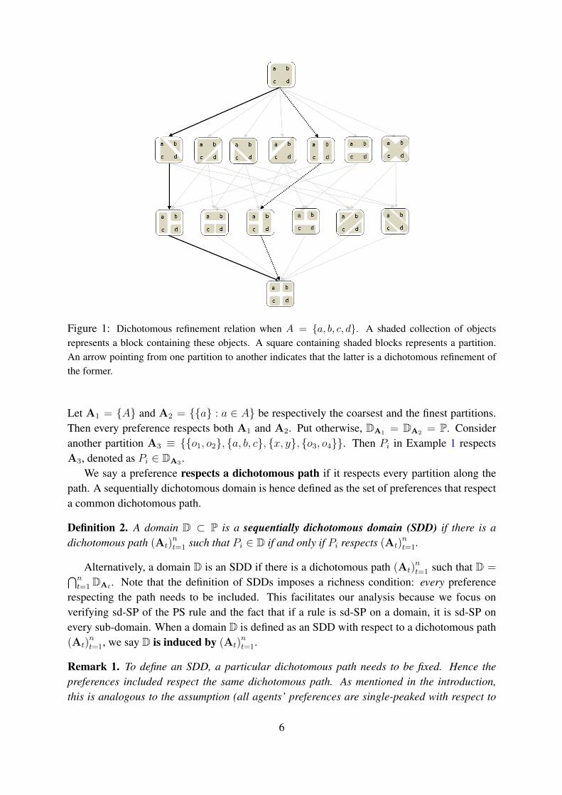
Figure 1: Dichotomous refinement relation when A = {a, b, c, d}. A shaded collection of objectsrepresents a block containing these objects. A square containing shaded blocks represents a partition.An arrow pointing from one partition to another indicates that the latter is a dichotomous refinement ofthe former.

Let A1 = {A} and A2 = {{a} : a ∈ A} be respectively the coarsest and the finest partitions.Then every preference respects both A1 and A2. Put otherwise, DA1 = DA2 = P. Consideranother partition A3 ≡ {{o1, o2}, {a, b, c}, {x, y}, {o3, o4}}. Then Pi in Example 1 respectsA3, denoted as Pi ∈ DA3 .

We say a preference respects a dichotomous path if it respects every partition along thepath. A sequentially dichotomous domain is hence defined as the set of preferences that respecta common dichotomous path.

Definition 2. A domain D ⊂ P is a sequentially dichotomous domain (SDD) if there is adichotomous path (At)

nt=1 such that Pi ∈ D if and only if Pi respects (At)

nt=1.

Alternatively, a domain D is an SDD if there is a dichotomous path (At)nt=1 such that D =⋂n

t=1 DAt . Note that the definition of SDDs imposes a richness condition: every preferencerespecting the path needs to be included. This facilitates our analysis because we focus onverifying sd-SP of the PS rule and the fact that if a rule is sd-SP on a domain, it is sd-SP onevery sub-domain. When a domain D is defined as an SDD with respect to a dichotomous path(At)

nt=1, we say D is induced by (At)

nt=1.

Remark 1. To define an SDD, a particular dichotomous path needs to be fixed. Hence thepreferences included respect the same dichotomous path. As mentioned in the introduction,this is analogous to the assumption (all agents’ preferences are single-peaked with respect to

6

the same linear order) that underlies the single-peaked domains. Continuing with the analogywith the single-peaked domain, the cardinality of an SDD coincides with the cardinality of thesingle-peaked domain. In particular, denoting by n the number of objects, both an SDD andthe single-peaked domain contain 2n−1 preferences. For instance, in Example 2, n = 4 and anSDD includes 8 preferences. �

Fixing a dichotomous path, the induced SDD is identified as the intersection of the domainsrespecting respectively the partitions in the path. The following are two examples of SDDs.

Example 2. Let A = {a, b, c, d}. We claim that the domain D ≡ {P1, · · · , P8} is an SDD,where the preferences are as follows.

P1 P2 P3 P4 P5 P6 P7 P8

a c d d b b b b

c a a c a c d d

d d c a c a a c

b b b b d d c a

In particular, we verify D =⋂4t=1 DAt , where (At)

4t=1 is a dichotomous path with A1 =

{{a, b, c, d}}, A2 = {{a, c, d}, {b}}, A3 = {{a, c}, {d}, {b}}, and A4 = {{a}, {c}, {d}, {b}}.This path is indicated by the darkened arrows in Figure 1.

First, since every preference respects A1 and A4, DA1 = DA4 = P. Second, a preferencerespects A2 if and only if b is ranked either at the top or at the bottom. Hence DA2 = {Pi ∈ P :

r1(Pi) = b or r4(Pi) = b}. Last, a preference Pi ∈ DA2 respects A3 if and only if {a, c} clustersin Pi. Hence DA2 ∩ DA3 = {Pi ∈ DA2 : {a, c} clusters in Pi}. In summary, D =

⋂4t=1 DAt .

Similarly, the domain D′ ≡ {P ′1, · · · , P ′8} is also an SDD. In particular, D′ is induced by(A′t)

4t=1, where A′1 = {{a, b, c, d}}, A′2 = {{a, c}, {b, d}}, A′3 = {{a}, {c}, {b, d}}, and

A′4 = {{a}, {c}, {b}, {d}}. This path is indicated by darkened and dotted arrows in Figure 1.

P ′1 P ′2 P ′3 P ′4 P ′5 P ′6 P ′7 P ′8

a c a c b d b d

c a c a d b d b

b b d d a a c c

d d b b c c a a

�

We provide in the following example an interpretation of the SDDs. One begins with aset of attributes and a linear order of them. Given an attribute, each object can be classifiedas either possessing the attribute or not. In particular, if an agent treats the first attribute asdesirable, every object possessing this attribute is better than every object that does not (andvice versa), and so on using the lexicographic rationale with respect to the pre-specified order.Thus, a dichotomous path is interpreted as the result of sequentially classifying the objects

7

according to the fixed order of attributes and the induced SDD is interpreted as being generatedby lexicographically expressing the desirability of the attributes.9 Example 3 below illustrates.

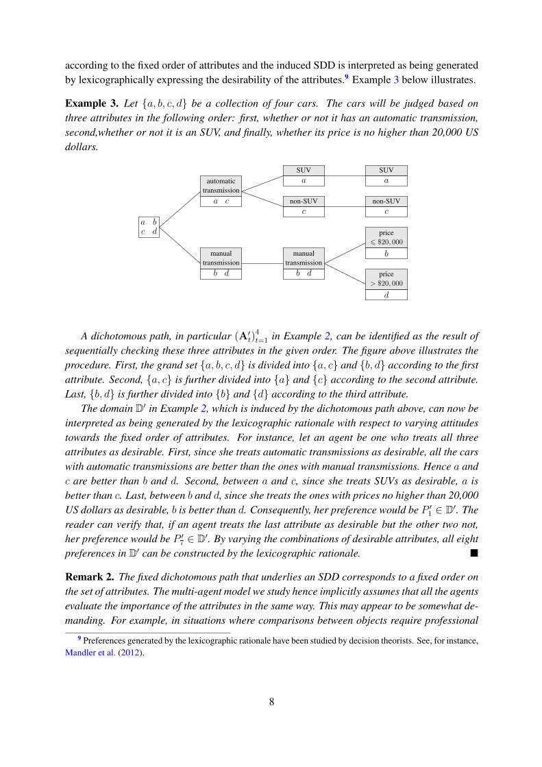
Example 3. Let {a, b, c, d} be a collection of four cars. The cars will be judged based onthree attributes in the following order: first, whether or not it has an automatic transmission,second,whether or not it is an SUV, and finally, whether its price is no higher than 20,000 USdollars.

a bc d

automatictransmissiona c

manualtransmissionb d

non-SUVc

SUVa

manualtransmissionb d

non-SUVc

SUVa

price6 $20, 000

b

price> $20, 000

d

A dichotomous path, in particular (A′t)4t=1 in Example 2, can be identified as the result of

sequentially checking these three attributes in the given order. The figure above illustrates theprocedure. First, the grand set {a, b, c, d} is divided into {a, c} and {b, d} according to the firstattribute. Second, {a, c} is further divided into {a} and {c} according to the second attribute.Last, {b, d} is further divided into {b} and {d} according to the third attribute.

The domain D′ in Example 2, which is induced by the dichotomous path above, can now beinterpreted as being generated by the lexicographic rationale with respect to varying attitudestowards the fixed order of attributes. For instance, let an agent be one who treats all threeattributes as desirable. First, since she treats automatic transmissions as desirable, all the carswith automatic transmissions are better than the ones with manual transmissions. Hence a andc are better than b and d. Second, between a and c, since she treats SUVs as desirable, a isbetter than c. Last, between b and d, since she treats the ones with prices no higher than 20,000US dollars as desirable, b is better than d. Consequently, her preference would be P ′1 ∈ D′. Thereader can verify that, if an agent treats the last attribute as desirable but the other two not,her preference would be P ′7 ∈ D′. By varying the combinations of desirable attributes, all eightpreferences in D′ can be constructed by the lexicographic rationale. �

Remark 2. The fixed dichotomous path that underlies an SDD corresponds to a fixed order onthe set of attributes. The multi-agent model we study hence implicitly assumes that all the agentsevaluate the importance of the attributes in the same way. This may appear to be somewhat de-manding. For example, in situations where comparisons between objects require professional

9 Preferences generated by the lexicographic rationale have been studied by decision theorists. See, for instance,Mandler et al. (2012).

8

inputs, this assumption requires that the agents refer to the same professional expert. In the cen-tralized allocation problems we consider, the authority who implements the assignment couldbe such an expert. �

In the next section we will show that the PS rule is sd-SP on any SDD. The verification ofsd-SP for a random assignment rule is in general a difficult task. In the following, we present akey feature of an SDD, which simplifies this task. In particular, it turns out that any deviation onan SDD can be decomposed as a sequence of preferences, where, between every two successivepreferences, exactly two adjacently ranked blocks are flipped. Such block flippings are calledblock-adjacent reversals and the preference resulting from a block-adjacent reversal is said tobe block-adjacent to the initial one.

Definition 3. A preference Pi is block-adjacent to Pi if there are two nonempty and disjointsubsets A1, A2 ⊂ A such that

1. A1, A2, and A1 ∪ A2 cluster in both Pi and Pi,

2. ∀ a, b ∈ A such that a ∈ A1 and b ∈ A2, a P0 b if and only if b P0 a,

3. ∀ a, b ∈ A such that either a 6∈ A1 or b 6∈ A2, a P0 b if and only if a P0 b.

Block-adjacency can be seen as a generalization of “adjacency” by Monjardet (2009), whichrefers to a pair of preferences which differ only in a flip between two adjacently ranked objects.It is important to note that a block-adjacent reversal between A1 and A2 does not change theranking of objects contained in A1, nor the ranking of objects contained in A2. This is capturedby the third requirement in the above definition.

The following example illustrates a decomposition of a deviation as a sequence of block-adjacent reversals.

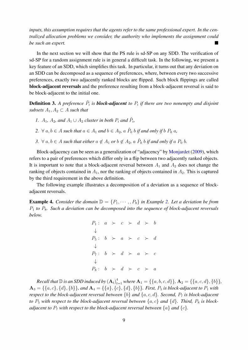
Example 4. Consider the domain D = {P1, · · · , , P8} in Example 2. Let a deviation be fromP1 to P8. Such a deviation can be decomposed into the sequence of block-adjacent reversalsbelow.

P1 : a � c � d � b

↓P5 : b � a � c � d

↓P7 : b � d � a � c

↓P8 : b � d � c � a

Recall that D is an SDD induced by (At)4t=1 where A1 = {{a, b, c, d}}, A2 = {{a, c, d}, {b}},

A3 = {{a, c}, {d}, {b}}, and A4 = {{a}, {c}, {d}, {b}}. First, P5 is block-adjacent to P1 withrespect to the block-adjacent reversal between {b} and {a, c, d}. Second, P7 is block-adjacentto P5 with respect to the block-adjacent reversal between {a, c} and {d}. Third, P8 is block-adjacent to P7 with respect to the block-adjacent reversal between {a} and {c}.

9

Note that these three reversals correspond to the dichotomous divisions along the dichoto-mous path. First, from A1 to A2, {a, b, c, d} breaks into {b} and {a, c, d}. Second, from A2 toA3, {a, c, d} breaks into {a, c} and {d}. Third, from A3 to A4, {a, c} breaks into {a} and {c}.In general, a deviation may not involve all the dichotomous divisions but a subset of them. Forexample, the deviation from P1 to P4 involves only two reversals: one between {a, c} and {d}and the other between {a} and {c}. �

The remainder of this section presents three remarks on the SDDs.

Remark 3. An SDD satisfies minimal richness, namely, for each a ∈ A, there is a preferencePi in the domain such that r1(Pi) = a. This is illustrated by the domains in Example 2. �

Remark 4. Two different dichotomous paths may induce the same SDD. Consider the domainD′ in Example 2. We have seen that this domain is an SDD induced by the dichotomous path(A′t)

4t=1. It turns out that D′ is also induced by (A′′t )

4t=1, where A′′3 ≡ {{a, c}, {b}, {d}} and

A′′t ≡ A′t for t = 1, 2, 4. However this non-uniqueness turns out to be inconsequential for ouranalysis. �

Remark 5. Liu and Zeng (2018) introduced the notion of a restricted tier domain and showedthat if a domain admits an sd-SP, sd-Eff, and ETE rule, then it is a subset of the union ofrestricted tier domains. A well-known fact about the PS rule is that it satisfies sd-Eff and ETEon any domain. We will show in Theorem 1 that the PS rule on an SDD is sd-SP. Then, asa corollary, an SDD can always be expressed as a subset of the union of some restricted tierdomains. To see this, we first introduce restricted tier domains. An ordered partition of A,denoted by P , is a restricted tier structure if each block contains at most two objects. Thecorresponding restricted tier domain, denoted by D(P), is then defined as the collection ofpreferences that respect the order of the blocks. Four restricted tier structures are listed below.

P1 P2 P3 P4

{a, c} {d} {b} {b}{d} {a, c} {a, c} {d}{b} {b} {d} {a, c}

The corresponding restricted tier domains are respectively D(P1) = {P1, P2}, D(P2) =

{P3, P4}, D(P3) = {P5, P6}, and D(P4) = {P7, P8}, where the involved preferences are fromExample 2. Recall that the set of these eight preferences is an SDD. Hence we have decomposedit as the union of four restricted tier domains. Generally, this decomposition can be identifiedby examining the dichotomous path that induces the given SDD. For details, see the extensionpart of Liu and Zeng (2018).

In addition, Liu and Zeng (2018) introduced a condition called the local elevating property.This condition requires the existence of three preferences, three objects, and three consecutivepositions such that (i) these three objects are ranked at these three positions in all three pref-erences, (ii) the set of objects ranked higher than these three positions is the same in all threepreferences, (iii) one of the three objects takes three different positions in three preferences andthe other two are ranked in the same way. They proved that if a domain admits a desirable rule,

10

it violates the local elevating property. By Theorem 1, an SDD admits a desirable rule. Thus itviolates the local elevating property. �

4 The PS Rule on Sequentially Dichotomous Domains

This section presents two main results. Theorem 1 shows that the PS rule is sd-strategy-proof on a sequentially dichotomous domain. Theorem 2 shows that a sequentially dichotomousdomain is maximal for the PS rule to be sd-strategy-proof.

Theorem 1 is proved by means of two lemmas. Recall that a deviation in an SDD canbe decomposed as a sequence of block-adjacent reversals. Accordingly, we define an incen-tive compatibility notion weaker than sd-SP, called block-adjacent sd-strategy-proofness. LetLi be agent i’s lottery when she reports her true preference. Let L′i be her lottery when shereports a different preference that is block-adjacent to the true one. Then block-adjacent sd-strategy-proofness requires that Li first-order stochastically dominates L′i according to her truepreference. Lemma 1 shows that, on an SDD, a rule is sd-SP if and only if it is block-adjacentsd-strategy-proof. Next, Lemma 2 implies block-adjacent sd-strategy-proofness of the PS rule.

We start the discussion from the formal definition of block-adjacent sd-strategy-proofness.

Definition 4. A rule ϕ : Dn → L is block-adjacent sd-strategy-proof (BA-sd-SP) if ∀ i ∈ I ,Pi, Pi ∈ D, and P−i ∈ Dn−1, such that Pi is block-adjacent to Pi, ϕi(Pi, P−i) P sd

i ϕi(Pi, P−i).

Although BA-sd-SP is a weaker condition than sd-SP, it turns out that these two conditionsare equivalent on an SDD. We present this fact below in Lemma 1. Example 5 illustrates theidea of the proof.

Example 5. Consider the deviation from P1 to P8 in Example 4. We have shown that thisdeviation can be decomposed as a sequence of block-adjacent reversals. Let L1, L5, L7, L8

denote respectively the deviating agent’s lottery when she reports P1, P5, P7, P8. Given BA-sd-SP, what we need to establish is L1 P

sd1 L8.

P1 : a � c � d � b

↓ L1 Psd1 L5 + L5 P

sd1 L7 + L7 P

sd1 L8 ⇒ L1 P

sd1 L8

P5 : b � a � c � d ⇑ ⇑

↓ L5 Psd5 L7

L7 Psd7 L5

L7 Psd5 L8

L7b = L8b

L7d = L8d

P7 : b � d � a � c ⇑

↓ L7 Psd7 L8

L8 Psd8 L7

P8 : b � d � c � a

First, by BA-sd-SP, we have L5 Psd5 L7 and L7 P

sd7 L5. These two statements together imply

L5b = L7b. Given this and the fact that P1 and P5 rank a, c, and d in the same way, L5 Psd5 L7

implies L5 Psd1 L7.

11

Second, by the same argument as above, BA-sd-SP implies L7b = L8b, L7d = L8d, andL7 P

sd5 L8. By noting that P1 and P5 rank a and c in the same way, we have further L7 P

sd1 L8.

Finally the transitivity of P sd1 establishes L1 P

sd1 L8. �

Lemma 1. On a sequentially dichotomous domain, a rule is sd-strategy-proof if and only if itis block-adjacent sd-strategy-proof.

The proof, which follows the logic illustrated in Example 5, is in Appendix A.Lemma 1 is related to the studies on the equivalence between local and global incentive com-

patibility. Sato (2013) focused on deterministic ordinal mechanisms, namely, mappings fromprofiles of ordinal preferences on a set of deterministic outcomes to these outcomes. Instancesinclude the deterministic voting rules and the deterministic allocation rules. He identified acondition, called non-restoration, and proved that if a domain satisfies this condition, a deter-ministic ordinal mechanism is strategy-proof if and only if it satisfies a local notion of incentivecompatibility. This notion is called AM-strategy-proofness and requires that a flip between twoadjacently ranked objects not lead to a better outcome. Cho (2016a) studied random ordinalmechanisms and proved that non-restoration is also sufficient for the equivalence between sd-SP and AM-sd-strategy-proofness, which requires that a flip between two adjacently rankedobjects not lead to a lottery which is not first-order stochastically dominated by the lottery de-livered by the original preference.10

The non-restoration property requires that between any two preferences, there is a sequenceof preferences connecting them such that (i) every pair of adjacent preferences differ only in aflip of two adjacently ranked objects, and (ii) along the sequence no pair of objects are flippedmore than once. An SDD violates the condition (i). To see this, note that between P2 and P3

in Example 2, there is no sequence of preferences in the given SDD satisfying (i). Hence theequivalence provided by Cho (2016a) cannot be used to simplify the verification of sd-SP onSDDs.

Block-adjacent reversals include as special cases the flips between adjacently ranked ob-jects. Hence BA-sd-SP is stronger than AM-sd-strategy-proofness. Although BA-sd-SP re-quires more, it still helps in the verification of sd-SP on SDDs.

Due to Lemma 1, to show sd-SP of the PS rule on an SDD, it suffices to show BA-sd-SP.Lemma 2 below asserts a slightly stronger property.

Lemma 2. Let P ∈ Pn, Pi ∈ P, if there are two nonempty and disjoint subsets of objectsA1, A2 ⊂ A such that

1. for all j ∈ I , A1, A2, and A1 ∪ A2 cluster in Pj ,

2. Pi is block-adjacent to Pi with respect to the reversal between A1 and A2,

3. ∀ a ∈ A1 and b ∈ A2, a P1 b and b P1 a,10In addition to the first-order stochastic dominance extension, Cho (2016a) studied two other extension meth-

ods. Independently, Carroll (2012) studied also the equivalence between local and global incentive compatibility.However, he examined the equivalence on specific preference domains, for instance, the single-peaked domain. Inaddition, he also investigated cardinal mechanisms.

12

then:

1. ∀ a ∈ A1, PS1a(P ) > PS1a(P1, P−1),

2. ∀ b ∈ A2, PS1b(P ) 6 PS1b(P1, P−1),

3. ∀ x ∈ A\A1 ∪ A2, PS1x(P ) = PS1x(P1, P−1).

The proof of Lemma 2 is in Appendix B.Lemma 2 says that if one agent performs a block-adjacent reversal between A1, A2 ⊂ A and

it is known that in every other’s preference A1, A2, and A1 ∪ A2 cluster, then for every objectthat has been moved downward in the deviator’s preference, the probability for the deviator toget this object is non-increasing. Note that there is no requirement on how the objects in A1 (orthe objects in A2) are ranked in Pj for j 6= i. It is evident that this lemma implies BA-sd-SP onan SDD.

The statement of Lemma 2 is stronger than the statement that the PS rule is BA-sd-SP on anSDD for two reasons. First, the lemma does not require the preferences to be taken from a givenSDD. Rather, the requirement is that A1, A2, and A1 ∪ A2 cluster in the preferences involved.Second, BA-sd-SP does not require the probability of every object that is moved downwardsto be non-increasing. Rather, it requires only the probability of every upper contour set to benon-increasing. For example, consider the block-adjacent deviation from a � b � c � d to c �a � b � d. BA-sd-SP requires that the probability of getting a, b combined be non-increasing.In particular, the probability of getting b is allowed to increase as long as the decrease in a’sprobability exceeds the increase in b’s probability. Although Lemma 2 states more than what isneeded to show the theorem, we still present it, in the hope that it may prove useful for furtherresearch.

We are now ready to present the theorem.

Theorem 1. The PS rule is sd-strategy-proof on a sequentially dichotomous domain.

The theorem follows directly from Lemma 1, and Lemma 2. By Lemma 2, the PS rule onan SDD is BA-sd-SP. Then by Lemma 1 the PS rule is sd-SP.

Given Theorem 1, the next question we ask is: Can we expand an SDD while preserving thesd-SP of PS rule? The answer is in the negative, as stated in Theorem 2.

Theorem 2. A sequentially dichotomous domain is maximal for the PS rule to be sd-strategy-proof.

The proof of Theorem 2 is in Appendix C. In the proof, we fix an arbitrary SDD, denoted byD, and an arbitrary preference P0 ∈ P\D. We first compare P0 with an arbitrary dichotomouspath which induces D. This allows us to identify two preferences in the SDD, P0, P0 ∈ D. Wethen construct two preference profiles consisting of only P0, P0, P0. In these two preferenceprofiles, one agent deviates. Finally we calculate the relevant probabilities specified by the PSrule and show that this deviation is profitable. The manipulability of the PS rule between the twoconstructed preference profiles is essentially the same as illustrated by the following example,although the proof is more complicated and involves the consideration of several cases.11

11This example is modified from the first example in Liu and Zeng (2018).

13

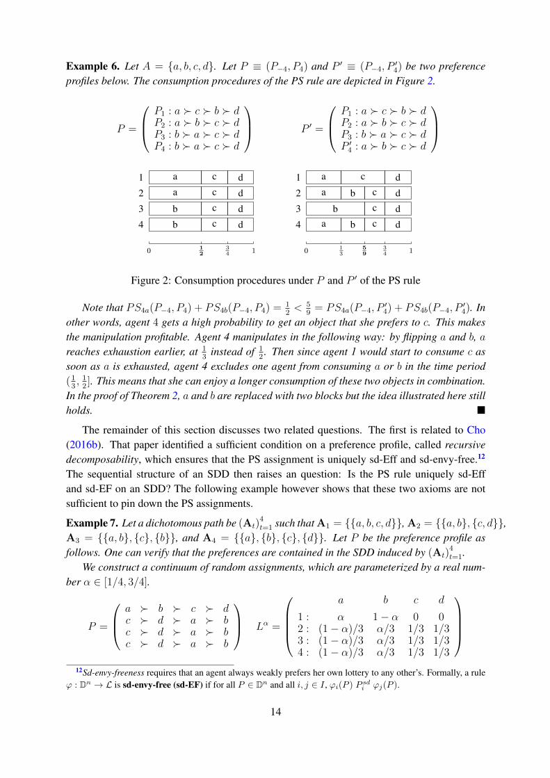
Example 6. Let A = {a, b, c, d}. Let P ≡ (P−4, P4) and P ′ ≡ (P−4, P′4) be two preference

profiles below. The consumption procedures of the PS rule are depicted in Figure 2.

P =

P1 : a � c � b � dP2 : a � b � c � dP3 : b � a � c � dP4 : b � a � c � d

P ′ =

P1 : a � c � b � dP2 : a � b � c � dP3 : b � a � c � dP ′4 : a � b � c � d

0 12

34 1

1

2

3

4

a c da c d

b c d

b c d

0 13

59

34 1

1

2

3

4

a c da b c d

b c da b c d

Figure 2: Consumption procedures under P and P ′ of the PS rule

Note that PS4a(P−4, P4) + PS4b(P−4, P4) = 12< 5

9= PS4a(P−4, P

′4) + PS4b(P−4, P

′4). In

other words, agent 4 gets a high probability to get an object that she prefers to c. This makesthe manipulation profitable. Agent 4 manipulates in the following way: by flipping a and b, areaches exhaustion earlier, at 1

3instead of 1

2. Then since agent 1 would start to consume c as

soon as a is exhausted, agent 4 excludes one agent from consuming a or b in the time period(1

3, 1

2]. This means that she can enjoy a longer consumption of these two objects in combination.

In the proof of Theorem 2, a and b are replaced with two blocks but the idea illustrated here stillholds. �

The remainder of this section discusses two related questions. The first is related to Cho(2016b). That paper identified a sufficient condition on a preference profile, called recursivedecomposability, which ensures that the PS assignment is uniquely sd-Eff and sd-envy-free.12

The sequential structure of an SDD then raises an question: Is the PS rule uniquely sd-Effand sd-EF on an SDD? The following example however shows that these two axioms are notsufficient to pin down the PS assignments.

Example 7. Let a dichotomous path be (At)4t=1 such that A1 = {{a, b, c, d}}, A2 = {{a, b}, {c, d}},

A3 = {{a, b}, {c}, {b}}, and A4 = {{a}, {b}, {c}, {d}}. Let P be the preference profile asfollows. One can verify that the preferences are contained in the SDD induced by (At)

4t=1.

We construct a continuum of random assignments, which are parameterized by a real num-ber α ∈ [1/4, 3/4].

P =

a � b � c � dc � d � a � bc � d � a � bc � d � a � b

Lα =

a b c d

1 : α 1− α 0 02 : (1− α)/3 α/3 1/3 1/33 : (1− α)/3 α/3 1/3 1/34 : (1− α)/3 α/3 1/3 1/3

12Sd-envy-freeness requires that an agent always weakly prefers her own lottery to any other’s. Formally, a rule

ϕ : Dn → L is sd-envy-free (sd-EF) if for all P ∈ Dn and all i, j ∈ I , ϕi(P ) P sdi ϕj(P ).

14

Note first that PS(P ) = L3/4. We show that an assignment L is sd-Eff and sd-EF at P ifand only if L ∈ {Lα : α ∈ [1/4, 3/4]}.

If: First, sd-EF can be verified by definition. We check sd-Eff. Suppose not, let L′ 6= L andL′ P sd L. We derive a contradiction for each of the following two cases. Case 1: L′1 6= L1.Then L′1 P sd

1 L1 implies L′1a > L1a = α and L′1c = L′1d = 0. Feasibility and L′i Psdi Li,

∀i = 2, 3, 4 then imply L′ic = Lic = 1/3, L′id = Lid = 1/3, and L′ia > Lia = (1 − α)/3, ∀i = 2, 3, 4. We have hence a contradiction to feasibility:

∑i∈I L

′ia >

∑i∈I Lia = 1. Case 2:

L′1 = L1. Then feasibility and L′i Psdi Li, ∀i = 2, 3, 4 imply L′i = Li, ∀i = 2, 3, 4, which is a

contradiction to L′ 6= L.Only if: Let L be sd-Eff and sd-EF. First sd-Eff implies either L1c = L1d = 0 or Lia =

Lib = 0 for all i = 2, 3, 4. Feasibility rules out the later case. Given L1c = L1d = 0, feasibilityand sd-EF imply Lic = Lid = 1/3 for all i = 2, 3, 4. Given this, feasibility and sd-EF furtherimply that L is in the form of Lα, with α ∈ [0, 1]. Finally, sd-EF requires α ∈ [1/4, 3/4]. Inparticular, L1 P

sd1 L2 implies α > 1/4 and L2 P

sd2 L1 implies α 6 3/4. �

The second question is whether the class of SDDs is uniquely maximal. Put otherwise, ifwe know that the PS rule is sd-SP on a given domain, can we structure it as a sub-domain of anSDD? The example below proves this to be wrong.

Example 8. Let n = 4 and let a domain D consist of the following two preferences.

P0 : a � b � c � d

P0 : c � a � d � b

It is not difficult to check that the PS rule is sd-SP on D. However D can never be a sub-domain of any SDD. The key is that we cannot find a binary partition that both P0 and P0

respect. �

Interestingly the pattern indicated by the preferences in the above example has been inves-tigated, for example Rossin and Bouvel (2006). It seems that the exclusion of the above patternis crucial for the computer either to generate permutations fast or to compare two sets of per-mutations fast. For CS studies, it is perfectly justified that the pattern is excluded artificially.However, there is no economically reasonable excuse, to my understanding, for excluding sucha pattern. Hence, although by excluding such a pattern, we might be able to establish theuniqueness of SDDs for the PS rule to be sd-SP, this exercise is of little economic interest.

5 Conclusion

We identified a class of domains, called sequentially dichotomous domains, and proved thatthe PS rule is sd-strategy-proof on any such domain. In addition, each of these domains ismaximal for the PS rule to be sd-strategy-proof.

We close the discussion by listing three questions for future research. First, are there in-teresting sets of axioms that characterize the PS rule on an SDD? Second, on an SDD, what isthe set of all sd-Eff and sd-EF rules? Finally, as mentioned in the introduction, there appears

15

to be some connection between the voting problem and the random assignment problem, whichdeserves further investigation.

Appendix

A Proof of Lemma 1

The necessity part is evident by definition. We prove the sufficiency part.Let D be an SDD and let (At)

nt=1 be a dichotomous path that induces D. In addition, let

ϕ : Dn → L be a BA-sd-SP rule. Let P ∈ Dn and P ′1 ∈ D\{P1}. In addition, let L ≡ ϕ(P )

and L′ ≡ ϕ(P ′1, P−1). It suffices to show L1 Psd1 L′1.

Along the dichotomous path from A1 to An, a block breaks into two smaller ones at eachstep. A preference P0 respecting the dichotomous path figures the ranking between the twoblocks in each step t = 2, · · · , n. (For t = 1, there is only one major block.) Recall that foreach t = 2, · · · , n, A(t−1)∗ breaks into At1 and At2. Without loss of generality, suppose a P1 b

for all t = 2, · · · , n, a ∈ At1, b ∈ At2. Consequently P1 6= P ′1 implies the existence of asubsequence {tγ}Γ

γ=1 ⊂ {t}nt=2 such that b P ′1 a for all γ = 1, · · · ,Γ, a ∈ Atγ1, b ∈ Atγ2.Let P10 ≡ P1. We define a sequence of preferences (P1γ)

Γγ=1 such that for each γ, (i) b P1γ a

if and only if a P1γ−1 b for all a ∈ Atγ1 and b ∈ Atγ2; and (ii) a P1γ b if and only if a P1γ−1 b

otherwise. That is, for each γ ∈ {1, · · · ,Γ}, the difference between P1γ and P1γ−1 is onlya reversal between the blocks Atγ1 and Atγ2. Hence each P1γ results from a block-adjacentreversal of P1γ−1. In addition, following this sequence of block-adjacent reversals, we approachP ′1 and in the end P1Γ = P ′1. Note that for each γ ∈ {1, · · · ,Γ}, P1γ ∈ D.

Correspondingly we denote Lγ ≡ PS(P1γ, P−1) for each γ = 1, · · · ,Γ. In the following,we fix γ and show Lγ−1

1 P sd1 Lγ1 , in two steps.

Step 1: Lγ−11 P sd

1γ−1 Lγ1 . Note that P1γ results from a block-adjacent reversal of P1γ−1. Then

BA-sd-SP establishes the step.Step 2: ∀α = 2, · · · , γ, Lγ−1

1 P sd1α−1 L

γ1 ⇒ Lγ−1

1 P sd1α−2 L

γ1 .

First note that, since α 6 γ, Atγ1, Atγ2, and Atγ1 ∪ Atγ2 cluster respectively in both P1α−1

and P1α−2. Note in addition that P1α−1 and P1α−2 differ only in block-adjacent reversal betweenAtα−11 and Atα−12. Note last that, by the definition of SDD, one of the following two casesoccurs.

Case 1:(Atγ1 ∪ Atγ2

)⊂ Atα−11 or

(Atγ1 ∪ Atγ2

)⊂ Atα−12. We show Lγ−1

1 P sd1α−1 L

γ1 ⇒

Lγ−11 P sd

1α−2 Lγ1 for the former sub-case and the argument applies to the latter sub-case as well.

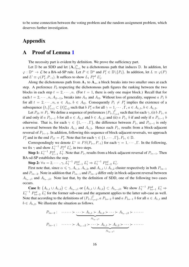
Note that according to the definitions of (P1γ)Γγ=1, a P1α−2 b and a P1α−1 b for all a ∈ Atγ1 and

b ∈ Atγ2. We illustrate the situation as follows.

P1α−2 : · · · · · · � · · · � Atγ1 � Atγ2 � · · ·︸ ︷︷ ︸Atα−11

� Atα−12 � · · · · · ·

P1α−1 : · · · · · · � Atα−12 � · · · � Atγ1 � Atγ2 � · · ·︸ ︷︷ ︸Atα−11

� · · · · · ·

16

Recall that BA-sd-SP implies that Lγ−11 and Lγ1 differ only in the assignments of the objects

in Atγ1 and Atγ2. In addition, by construction, the ranking of the objects within these twoblocks is the same in P1α−2 and P1α−1. Then by definition of first-order stochastic dominance,Lγ−1

1 P sd1α−1 L

γ1 ⇒ Lγ−1

1 P sd1α−2 L

γ1 .

Case 2:(Atγ1 ∪ Atγ2

)∩(Atα−11 ∪ Atα−12

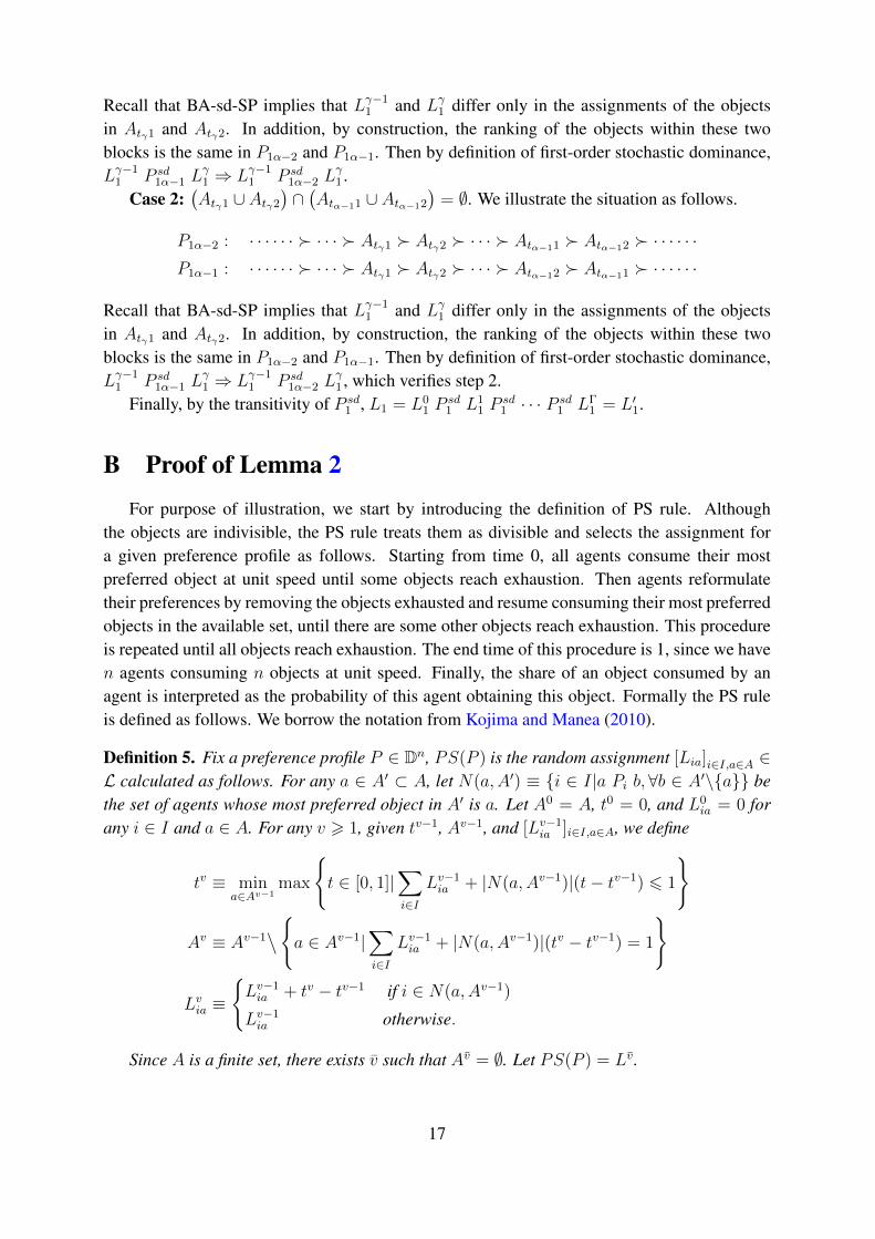
)= ∅. We illustrate the situation as follows.

P1α−2 : · · · · · · � · · · � Atγ1 � Atγ2 � · · · � Atα−11 � Atα−12 � · · · · · ·P1α−1 : · · · · · · � · · · � Atγ1 � Atγ2 � · · · � Atα−12 � Atα−11 � · · · · · ·

Recall that BA-sd-SP implies that Lγ−11 and Lγ1 differ only in the assignments of the objects

in Atγ1 and Atγ2. In addition, by construction, the ranking of the objects within these twoblocks is the same in P1α−2 and P1α−1. Then by definition of first-order stochastic dominance,Lγ−1

1 P sd1α−1 L

γ1 ⇒ Lγ−1

1 P sd1α−2 L

γ1 , which verifies step 2.

Finally, by the transitivity of P sd1 , L1 = L0

1 Psd1 L1

1 Psd1 · · · P sd

1 LΓ1 = L′1.

B Proof of Lemma 2

For purpose of illustration, we start by introducing the definition of PS rule. Althoughthe objects are indivisible, the PS rule treats them as divisible and selects the assignment fora given preference profile as follows. Starting from time 0, all agents consume their mostpreferred object at unit speed until some objects reach exhaustion. Then agents reformulatetheir preferences by removing the objects exhausted and resume consuming their most preferredobjects in the available set, until there are some other objects reach exhaustion. This procedureis repeated until all objects reach exhaustion. The end time of this procedure is 1, since we haven agents consuming n objects at unit speed. Finally, the share of an object consumed by anagent is interpreted as the probability of this agent obtaining this object. Formally the PS ruleis defined as follows. We borrow the notation from Kojima and Manea (2010).

Definition 5. Fix a preference profile P ∈ Dn, PS(P ) is the random assignment [Lia]i∈I,a∈A ∈L calculated as follows. For any a ∈ A′ ⊂ A, let N(a,A′) ≡ {i ∈ I|a Pi b,∀b ∈ A′\{a}} bethe set of agents whose most preferred object in A′ is a. Let A0 = A, t0 = 0, and L0

ia = 0 forany i ∈ I and a ∈ A. For any v > 1, given tv−1, Av−1, and [Lv−1

ia ]i∈I,a∈A, we define

tv ≡ mina∈Av−1

max

{t ∈ [0, 1]|

∑i∈I

Lv−1ia + |N(a,Av−1)|(t− tv−1) 6 1

}

Av ≡ Av−1∖{

a ∈ Av−1|∑i∈I

Lv−1ia + |N(a,Av−1)|(tv − tv−1) = 1

}

Lvia ≡

{Lv−1ia + tv − tv−1 if i ∈ N(a,Av−1)

Lv−1ia otherwise.

Since A is a finite set, there exists v such that Av = ∅. Let PS(P ) = Lv.

17

Fix a preference profile P , we call the sequence generated by applying the PS rule to P ,denoted by E ≡ (tv, Av, Lv)vv=0, the corresponding consumption procedure. Evidently, foreach v ∈ {0, · · · , v}, Av is the collection of objects which are still available at time tv. In otherwords, if a ∈ Av−1\Av, then a is available at tv−1 and reaches exhaustion at tv. For each a ∈ A,let ta ≡ tv where a ∈ Av−1\Av denote the time at which a reaches exhaustion.

Recall that an SDD is an intersection of domains, each of which respects a partition. Thenfor a better understanding of the consumption procedure specified by the PS rule when thepreferences belong to an SDD, we investigate the consumption procedure subject to a givenpartition.

Given a preference profile P ∈ DnA, every block in A clusters in every agent’s preference.

Let for instance {a, b} ∈ A be a block, then for every agent either a is ranked just above bor b is ranked just above a. Hence if a reaches exhaustion before b (ta < tb), the agents whoprefer a to b switch from a to b at ta while all the others keep consuming b until tb. If insteadb reaches exhaustion before a (tb < ta), then the agents who prefer b to a switch from b to aat tb and all the others keep consuming a until ta. Consequently, if we focus on only blocksrather than objects, we can ignore the time at which a reaches exhaustion if this occurs before band ignore the time at which b reaches exhaustion if this occurs before a. In other words, whatwe care about is only the time at which the whole block reaches exhaustion. For the examplehere, we need only to identify max{ta, tb}. Formally, the consumption procedure subject toA, denoted as E

∣∣A≡(tv∣∣A, Av∣∣A, Lv∣∣A

), is defined as follows.

Let V∣∣A≡ {v ∈ {0, · · · , v}|∃Ak ∈ A s.t. tv = maxa∈Ak ta} be the collection of time

points at which a block reaches exhaustion.

• tv∣∣A

is the subsequence of (tv)vv=0 involving elements in V∣∣A

. We record only the timepoints at which a block in A reaches exhaustion.

• Av∣∣A

is the subsequence of (Av)vv=0 involving elements in V∣∣A

.

• Lv∣∣A

is a matrix [LviAk ]i∈I,Ak∈A defined only for elements in V∣∣A

, whereLviAk ≡∑

a∈Ak Lvia.

When we focus on the consumption procedure subject to a partition, an important obser-vation is that the consumption procedure subject to A should not change when the preferenceprofile is changing in a way that the “ranking” of the blocks remain the same. That is, the changeinvolves only permutations within blocks won’t change the consumption procedure subject tothe partition. Here is an example.

Example 9. Let P ≡ (P1, P2, P5, P6) and P ≡ (P3, P2, P5, P6) where the preferences are fromExample 2. The consumption procedures of two profiles are illustrated as follows.

1:

2:

3:

4:0 1/2 3/4 1

a a d

c c d

b a d

b c d

1:

2:

3:

4:0 1/2 3/4 1

d d d

c c a

b a a

b c a

18

Recall that the involved preferences respect A2 = {{a, c, d}, {b}}. In addition the con-sumption procedure subject to A2 = {{a, c, d}, {b}} is not changing: In time interval (0, 1/2]

agents 1 and 2 consume objects in block {a, c, d} and agents 3 and 4 consume {b}. Then in timeinterval (1/2, 1] all agent consume objects in {a, c, d}. �

We formalize the observation illustrated in Example 9. Given a partition A, a preferencerespecting it, P0 ∈ DA, induces a (strict) preference on A in a natural way: a block is said tobe ranked above another block if every object in the former is ranked above every object in thelatter. Given a partition A, P(A) denotes the collection of all strict preferences on A.

Definition 6. Fixing a partition A, a preference on blocks PA0 ∈ P(A) is induced by P0 ∈ DA

if, ∀ Ak, Al ∈ A, [Ak PA0 Al]⇔ [∀a ∈ Ak, b ∈ Al, a P0 b].

Evidently, a preference P0 ∈ DA induces a unique preference PA0 on A. However the

converse is not true: two different preferences P0, P′0 ∈ DA may induce the same preference

PA0 on A. For example, preferences P1 and P3 in Example 2 induce the same preference on

A2: {a, c, d} � {b}.Now we formalize the observation in Example 9 as the following lemma.

Lemma 3. For P, P ∈ DnA such that PA

i = PAi for all i ∈ I , the consumption procedures

subject to A for two preference profiles are the same, namely E∣∣A

= E∣∣A

. This implies also∑a∈Ak PSia(P ) =

∑a∈Ak PSia(P ) for all i ∈ I and Ak ∈ A.

We are now ready to prove Lemma 2.Let L ≡ PS(P ) and L ≡ PS(P1, P−1). Let E ≡ (tv, Av, [Lvia]i∈I,a∈A)vv=0 and E ≡(

tv, Av, [Lvia]i∈I,a∈A

)¯v

v=0be respectively consumption procedures for P and (P1, P−1). In addi-

tion, let B ≡ {a ∈ A|a P1 x,∀x ∈ A1 ∪ A2} and C ≡ A\ (A ∪ A1 ∪ A2) be respectively theupper and lower contour sets of objects in A1 ∪ A2 according to P1. Evidently, these two setsare the same for P1.

Before proceeding to the proof, we clarify some notation.

• For each a ∈ A, let ta and ta denote respectively the times at which a reaches exhaustionin E and E .

• For each D ⊂ A, let tD ≡ max{ta : a ∈ D} and tD ≡ max{ta : a ∈ D} be respectivelythe times at which D reaches exhaustion in E and E .

• For each a ∈ A and v ∈ {0, 1, · · · , v}, let Sa(tv) ≡ 1−∑

i∈I Lvia be what remains of a at

time tv in E . Similarly, for each a ∈ A and v ∈ {0, 1, · · · , ¯v}, let Sa(tv) ≡ 1−∑

i∈I Lvia

be what remains of a at time tv in E .

We prove the lemma in three steps.Step 1: L1a = L1a for all a ∈ A\ (A1 ∪ A2).Consider a partition A ≡ {A1 ∪ A2, {a} : a ∈ A\ (A1 ∪ A2)}. Since P1 and P1 differ only

in a flip between A1 and A2, PA1 = PA

1 . Then, by Lemma 3, we are done. In addition, byLemma 3, we have the following facts.

19

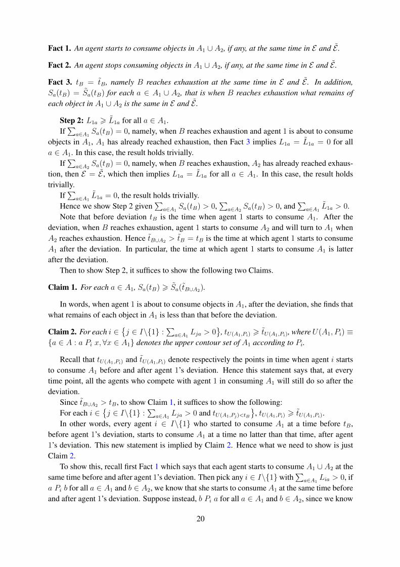
Fact 1. An agent starts to consume objects in A1 ∪ A2, if any, at the same time in E and E .

Fact 2. An agent stops consuming objects in A1 ∪ A2, if any, at the same time in E and E .

Fact 3. tB = tB, namely B reaches exhaustion at the same time in E and E . In addition,Sa(tB) = Sa(tB) for each a ∈ A1 ∪ A2, that is when B reaches exhaustion what remains ofeach object in A1 ∪ A2 is the same in E and E .

Step 2: L1a > L1a for all a ∈ A1.If∑

a∈A1Sa(tB) = 0, namely, when B reaches exhaustion and agent 1 is about to consume

objects in A1, A1 has already reached exhaustion, then Fact 3 implies L1a = L1a = 0 for alla ∈ A1. In this case, the result holds trivially.

If∑

a∈A2Sa(tB) = 0, namely, when B reaches exhaustion, A2 has already reached exhaus-

tion, then E = E , which then implies L1a = L1a for all a ∈ A1. In this case, the result holdstrivially.

If∑

a∈A1L1a = 0, the result holds trivially.

Hence we show Step 2 given∑

a∈A1Sa(tB) > 0,

∑a∈A2

Sa(tB) > 0, and∑

a∈A1L1a > 0.

Note that before deviation tB is the time when agent 1 starts to consume A1. After thedeviation, when B reaches exhaustion, agent 1 starts to consume A2 and will turn to A1 whenA2 reaches exhaustion. Hence tB∪A2 > tB = tB is the time at which agent 1 starts to consumeA1 after the deviation. In particular, the time at which agent 1 starts to consume A1 is latterafter the deviation.

Then to show Step 2, it suffices to show the following two Claims.

Claim 1. For each a ∈ A1, Sa(tB) > Sa(tB∪A2).

In words, when agent 1 is about to consume objects in A1, after the deviation, she finds thatwhat remains of each object in A1 is less than that before the deviation.

Claim 2. For each i ∈{j ∈ I\{1} :

∑a∈A1

Lja > 0}

, tU(A1,Pi) > tU(A1,Pi), whereU(A1, Pi) ≡{a ∈ A : a Pi x, ∀x ∈ A1} denotes the upper contour set of A1 according to Pi.

Recall that tU(A1,Pi) and tU(A1,Pi) denote respectively the points in time when agent i startsto consume A1 before and after agent 1’s deviation. Hence this statement says that, at everytime point, all the agents who compete with agent 1 in consuming A1 will still do so after thedeviation.

Since tB∪A2 > tB, to show Claim 1, it suffices to show the following:For each i ∈

{j ∈ I\{1} :

∑a∈A1

Lja > 0 and tU(A1,Pj)<tB

}, tU(A1,Pi) > tU(A1,Pi).

In other words, every agent i ∈ I\{1} who started to consume A1 at a time before tB,before agent 1’s deviation, starts to consume A1 at a time no latter than that time, after agent1’s deviation. This new statement is implied by Claim 2. Hence what we need to show is justClaim 2.

To show this, recall first Fact 1 which says that each agent starts to consume A1 ∪ A2 at thesame time before and after agent 1’s deviation. Then pick any i ∈ I\{1}with

∑a∈A1

Lia > 0, ifa Pi b for all a ∈ A1 and b ∈ A2, we know that she starts to consumeA1 at the same time beforeand after agent 1’s deviation. Suppose instead, b Pi a for all a ∈ A1 and b ∈ A2, since we know

20

this agent starts to consume A1 immediately when all the objects in A2 reach exhaustion, whatwe need to show is just tB∪A2 > tB∪A2 . This can be seen from the consumption proceduresfor P and (P1, P−1) subject to the partition {A1, A2, {a ∈ A : a 6∈ A1 ∪ A2}}. Hence wehave shown that for each i ∈ I\{1} with

∑a∈A1

Lia > 0, if she prefers A1 to A2, she starts toconsume A1 at the same time before and after the deviation; if she prefers A2 to A1, she startsto consume A1 after the deviation at a time earlier than before deviation, which proves Step 2.

Step 3: L1a 6 L1a for all a ∈ A2.By exchanging the roles of P1 and P1, Step 3 is implied by Step 2.

C Proof of Theorem 2

Let D be an SDD and let (At)nt=1 be a corresponding dichotomous path. Let P0 ∈ P\D be

an arbitrary preference not in D, we show that the PS rule defined on the union of D and P0 ismanipulable. Formally, the rule is a mapping PS :

(D ∪ {P0}

)n→ L.

Since D =⋃nt=1 DAt and P0 6∈ D, t ≡ min{t ∈ {1, · · · , n} : P0 6∈ DAt} is well-defined.

In addition, since P0 respects A1 = {A} trivially, t > 2. Recall that from At−1 to At, A(t−1)∗

breaks into At1 and At2. Let a ≡ r1(P0, A(t−1)∗) be the most preferred objects according to P0

in A(t−1)∗. Without loss of generality, let a ∈ At1. In addition, let c ≡ r1(P0, At2) be the mostpreferred objects according to P0 in At2. Since P0 does not respect At, there is b ∈ At1\{a}ranked below c. Let b ≡ r1(P0, {x ∈ At1 : c P0 x}) be the most preferred object in At1 thatis ranked below c. In addition, let C ≡ {x ∈ At1\{a} : x P0 c}. Note that C may be empty.Hence P0 can be illustrated as follows.

P0 : · · · · · · �A(t−1)∗︷ ︸︸ ︷

a � · · ·C · · ·︸ ︷︷ ︸⊂At1

� c � · · ·︸ ︷︷ ︸⊂At2

� b � · · ·︸ ︷︷ ︸⊂At1

� · · · · · · � · · · · · ·

There is a unique t > t such that a, b ∈ A(t−1)∗, a ∈ At1, and b ∈ At2 In other words, fromAt−1 to At, a and b are split into two separate blocks. Let B ≡ At1\{a} and D ≡ At2\{b}.Note that B and D may be empty.

In the following, we identify two preferences P0, P0 ∈ D. Then we construct two preferenceprofiles consisting of only P0, P0 and P0 and show that there is a profitable manipulation. Todo this, we need to consider four cases.

Case 1: C = ∅ or r1(P0, C) 6∈ B ∪D.Since P0 respects At−1, PAt−1

0 is well-defined. Let PAt−1

0 = PAt−1

0 = PAt−1

0 . Second, letA(t−1)∗ be the first-ranked block in At−1 according to both P0 and P0. Third, let At1P

At0 At2 and

At2PAt0 At1. Fourth, let a be the first-ranked object in At1 and b the first-ranked object in At2

according to both P0 and P0. Last, let P0 and P0 rank the objects contained in the same blockin the same way. It is evident that P0, P0 ∈ D. Hence, P0 and P0 are illustrated below.

21

P0 : · · · · · · �=At1︷ ︸︸ ︷

a � · · ·B · · · �=At2︷ ︸︸ ︷

b � · · ·D · · · � · · ·︸ ︷︷ ︸=At1

� c · · · · · ·︸ ︷︷ ︸=At2

� · · · · · ·

P0 : · · · · · · �=At2︷ ︸︸ ︷

b � · · ·D · · · �=At1︷ ︸︸ ︷

a � · · ·B · · · � · · ·︸ ︷︷ ︸=At1

� c · · · · · ·︸ ︷︷ ︸=At2

� · · · · · ·

Let P ≡ (P1, P2, P3, · · · , Pn) and P ′ ≡ (P1, P2, P3, · · · , Pn). We calculate the probabilitiesspecified by the PS rule as follows.

PS(P ) : a B b D

1 : 1n

0 0 0

2 · · ·n : 1n

|B|n−1

1n−1

|D|n−1

For P , all agents share a equally. Then agents 2 to n consume B ∪ {b} ∪D while agent 1

consumes c if C is empty and r1(P0, C) if not. Since the PS assignment is sd-Eff, PS(P )1x = 0

for all x ∈ B ∪ {b} ∪D. Then the ETE of PS assignment determines the other entries.

PS(P ′) : a B b D

1 : 1n−1

0 0 0

2 : 0 0 1n−1

+ |B|n−2

+1− 1

n−1− |B|n−2

n−1|D|n−1

3 · · ·n : 1n−1

|B|n−2

1− 1n−1− |B|n−2

n−1|D|n−1

For P ′, agents other than 2 share a equally. By sd-Eff, PS(P )1x = 0 for all x ∈ B∪{b}∪D.During the period when agents other than 2 consume a, agent 2 consumes b. When a reachesexhaustion, agents 3 to n start to consume B if B is nonempty and b if not; agent 1 starts toconsume c if C is empty and r1(P0, C) if not; and agent 2 still consumes b. It is evident that Bwill reach exhaustion before b or r1(P0, C). Then agents 3 to n join agent 2 in consuming b, sothey share equally what remains of b. In particular, 1− 1

n−1− |B|

n−2of b. Last, agents 2 to n share

D equally.Now we have a contradiction to sd-SP:

sd-SP⇒∑

x∈{a,b}∪B∪D

PS2x(P ) =∑

x∈{a,b}∪B∪D

PS2x(P ′)

⇒ 1

n+|B|n− 1

+1

n− 1+|D|n− 1

=1

n− 1+|B|n− 2

+1− 1

n−1 −|B|n−2

n− 1+|D|n− 1

⇒ 1

n(n− 1)2= 0 : contradiction.

Case 2: r1(P0, C) ∈ B.In order to identify a contradiction, we need to consider two sub-cases. Given r1(P0, C) ∈

B, there is an upper contour set in C contained in B. Let B1 be the largest such upper contour

22

set. Formally, B1 ≡ maxk6|C|{Uk(P0, C) ⊂ B}13. Hence either B1 = C or r1(P0, C\B1)

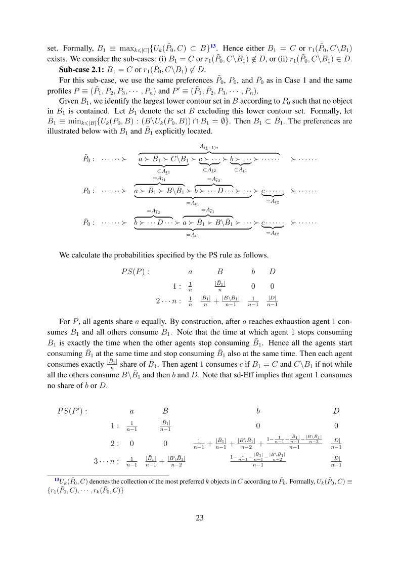
exists. We consider the sub-cases: (i) B1 = C or r1(P0, C\B1) 6∈ D, or (ii) r1(P0, C\B1) ∈ D.Sub-case 2.1: B1 = C or r1(P0, C\B1) 6∈ D.For this sub-case, we use the same preferences P0, P0, and P0 as in Case 1 and the same

profiles P ≡ (P1, P2, P3, · · · , Pn) and P ′ ≡ (P1, P2, P3, · · · , Pn).Given B1, we identify the largest lower contour set in B according to P0 such that no object

in B1 is contained. Let B1 denote the set B excluding this lower contour set. Formally, letB1 ≡ mink6|B|{Uk(P0, B) : (B\Uk(P0, B)) ∩ B1 = ∅}. Then B1 ⊂ B1. The preferences areillustrated below with B1 and B1 explicitly located.

P0 : · · · · · · �

A(t−1)∗︷ ︸︸ ︷a � B1 � C\B1︸ ︷︷ ︸

⊂At1

� c � · · ·︸ ︷︷ ︸⊂At2

� b � · · ·︸ ︷︷ ︸⊂At1

� · · · · · · � · · · · · ·

P0 : · · · · · · �

=At1︷ ︸︸ ︷a � B1 � B\B1 �

=At2︷ ︸︸ ︷b � · · ·D · · · � · · ·︸ ︷︷ ︸

=At1

� c · · · · · ·︸ ︷︷ ︸=At2

� · · · · · ·

P0 : · · · · · · �=At2︷ ︸︸ ︷

b � · · ·D · · · �

=At1︷ ︸︸ ︷a � B1 � B\B1 � · · ·︸ ︷︷ ︸

=At1

� c · · · · · ·︸ ︷︷ ︸=At2

� · · · · · ·

We calculate the probabilities specified by the PS rule as follows.

PS(P ) : a B b D

1 : 1n

|B1|n

0 0

2 · · ·n : 1n

|B1|n

+ |B\B1|n−1

1n−1

|D|n−1

For P , all agents share a equally. By construction, after a reaches exhaustion agent 1 con-sumes B1 and all others consume B1. Note that the time at which agent 1 stops consumingB1 is exactly the time when the other agents stop consuming B1. Hence all the agents startconsuming B1 at the same time and stop consuming B1 also at the same time. Then each agentconsumes exactly |B1|

nshare of B1. Then agent 1 consumes c if B1 = C and C\B1 if not while

all the others consume B\B1 and then b and D. Note that sd-Eff implies that agent 1 consumesno share of b or D.

PS(P ′) : a B b D

1 : 1n−1

|B1|n−1

0 0

2 : 0 0 1n−1

+ |B1|n−1

+ |B\B1|n−2

+1− 1

n−1− |B1|n−1− |B\B1|

n−2

n−1|D|n−1

3 · · ·n : 1n−1

|B1|n−1

+ |B\B1|n−2

1− 1n−1− |B1|n−1− |B\B1|

n−2

n−1|D|n−1

13Uk(P0, C) denotes the collection of the most preferred k objects inC according to P0. Formally, Uk(P0, C) ≡{r1(P0, C), · · · , rk(P0, C)}

23

For P ′, all agents other than 2 share a equally and at the same time agent 2 consumes b.Then agents other than 2 share B1 equally and agent 2 still consumes b. Then agent 1 starts toconsume c if C = B1 and C\B1 if not and agents 3 to n share B\B1 equally. During this timeperiod agent 2 is still consuming b. Then all agents other than 1 share equally what remains ofb, and D after b reaches exhaustion. The zero entries in the above table are implied by sd-Eff.

Now we have a contradiction to sd-SP:

sd-SP⇒∑

x∈{a,b}∪B∪D

PS2x(P ) =∑

x∈{a,b}∪B∪D

PS2x(P ′)

⇒ 1

n+|B1|n

+|B\B1|n− 1

+1

n− 1+|D|n− 1

=1

n− 1+|B1|n− 1

+|B\B1|n− 2

+1− 1

n−1 −|B1|n−1 −

|B\B1|n−2

n− 1+|D|n− 1

⇒ 1 + |B1|n(n− 1)2

= 0 : contradiction.

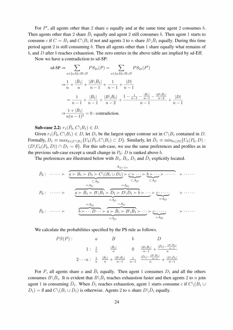
Sub-case 2.2: r1(P0, C\B1) ∈ D.Given r1(P0, C\B1) ∈ D, let D1 be the largest upper contour set in C\B1 contained in D.

Formally, D1 ≡ maxk6|C\B1|{Uk(P0, C\B1) ⊂ D}. Similarly, let D1 ≡ mink6|D|{Uk(P0, D) :

(D\Uk(P0, D)) ∩ D1 = ∅}. For this sub-case, we use the same preferences and profiles as inthe previous sub-case except a small change in P0: D is ranked above b.

The preferences are illustrated below with B1, B1, D1 and D1 explicitly located.

P0 : · · · · · · �

A(t−1)∗︷ ︸︸ ︷a � B1 � D1 � C\(B1 ∪D1)︸ ︷︷ ︸

⊂At1

� c � · · ·︸ ︷︷ ︸⊂At2

� b � · · ·︸ ︷︷ ︸⊂At1

� · · · · · · � · · · · · ·

P0 : · · · · · · �

=At1︷ ︸︸ ︷a � B1 � B\B1 �

=At2︷ ︸︸ ︷D1 � D\D1 � b � · · ·︸ ︷︷ ︸

=At1

� c · · · · · ·︸ ︷︷ ︸=At2

� · · · · · ·

P0 : · · · · · · �=At2︷ ︸︸ ︷

b � · · ·D · · · �

=At1︷ ︸︸ ︷a � B1 � B\B1 � · · ·︸ ︷︷ ︸

=At1

� c · · · · · ·︸ ︷︷ ︸=At2

� · · · · · ·

We calculate the probabilities specified by the PS rule as follows.

PS(P ) : a B b D

1 : 1n

|B1|n

0 |B\B1|n−1

+|D1|− |B\B1|

n−1

n

2 · · ·n : 1n

|B1|n

+ |B\B1|n−1

1n−1

|D1|− |B\B1|n−1

n+ |D\D1|

n−1

For P , all agents share a and B1 equally. Then agent 1 consumes D1 and all the othersconsumes B\B1. It is evident that B\B1 reaches exhaustion faster and then agents 2 to n joinagent 1 in consuming D1. When D1 reaches exhaustion, agent 1 starts consume c if C\(B1 ∪D1) = ∅ and C\(B1 ∪D1) is otherwise. Agents 2 to n share D\D1 equally.

24

PS(P ′) :

a B b D

1 : 1n−1

|B1|n−1 0 |B\B1|

n−2 +|D1|− |B\B1|

n−2

n−1

2 : 0 0 α+ 1−αn−1 0

3 · · ·n : 1n−1

|B1|n−1 + |B\B1|

n−21−αn−1

|D1|− |B\B1|n−2

n−1 + |D\D1|n−2

where α = 1n−1 + |B1|

n−1 + |B\B1|n−2 +

|D1|− |B\B1|n−2

n−1 + |D\D1|n−2 .

For P ′, agents other than 2 share a equally. When they consume a, agent 2 consumes b.After a reaches exhaustion, agents other than 2 share B1 equally and agent 2 still consumesb. After B1 reaches exhaustion, agent 1 consumes D1, agents 3 to n share B\B1 equally, andagent 2 still consumes b. It is evident that B\B1 reaches exhaustion faster. Then agents otherthan 2 share equally what remains of D1 and agent 2 still consumes b. Then agent 1 consumesc if C\(B1 ∪ D1) = ∅ and C\(B1 ∪ D1) if otherwise, agents 3 to n share D\D1 equally, andagent 2 still consumes b. Then agents other than 1 consume what remains of b.

Now we have a contradiction to sd-SP:

sd-SP⇒∑

x∈{a,b}∪B∪D

PS2x(P ) =∑

x∈{a,b}∪B∪D

PS2x(P ′)

⇒ 1

n+|B1|n

+|B\B1|n− 1

+1

n− 1+|D1| − |B\B1|

n−1

n+|D\D1|n− 1

= α+1− αn− 1

⇒|B1|+ |B\B1|+ |D1|+ 1

n(n− 1)2= 0 : contradiction.

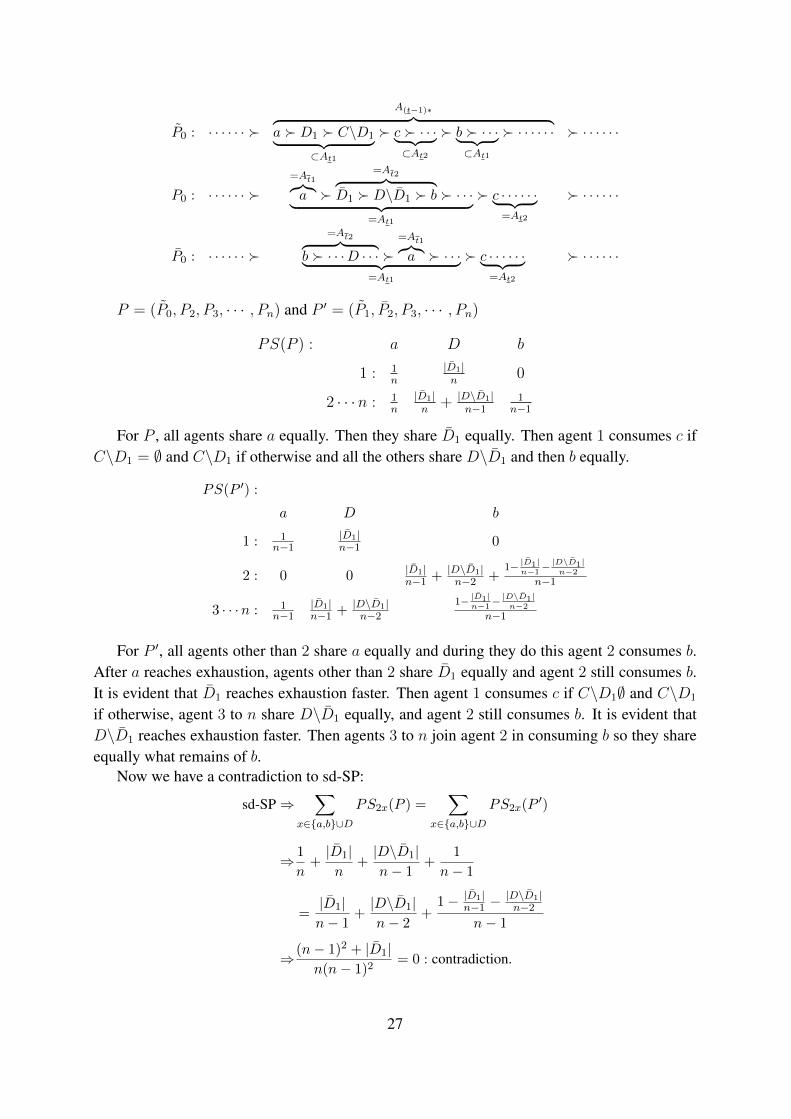
Case 3: r1(P0, C) ∈ D and B 6= ∅.Given r1(P0, C) ∈ D, letD1 be the largest upper contour set in C contained inD. Formally,

D1 ≡ maxk6|C|{Uk(P0, C) ⊂ D}. Similarly, let D1 ≡ mink6|D|{Uk(P0, D) : (D\Uk(P0, D))∩D1 = ∅}. For this sub-case, we use the same preferences and profiles as in Case 1.

For the reader to understand the consumption procedure better, preferences are illustratedbelow and D1 and D1 are explicitly located.

P0 : · · · · · · �

A(t−1)∗︷ ︸︸ ︷a � D1 � C\D1︸ ︷︷ ︸

⊂At1

� c � · · ·︸ ︷︷ ︸⊂At2

� b � · · ·︸ ︷︷ ︸⊂At1

� · · · · · · � · · · · · ·

P0 : · · · · · · �=At1︷ ︸︸ ︷

a � · · ·B · · · �

=At2︷ ︸︸ ︷b � D1 � D\D1 � · · ·︸ ︷︷ ︸

=At1

� c · · · · · ·︸ ︷︷ ︸=At2

� · · · · · ·

P0 : · · · · · · �

=At2︷ ︸︸ ︷b � D1 � D\D1 �

=At1︷ ︸︸ ︷a � · · ·B · · · � · · ·︸ ︷︷ ︸

=At1

� c · · · · · ·︸ ︷︷ ︸=At2

� · · · · · ·

25

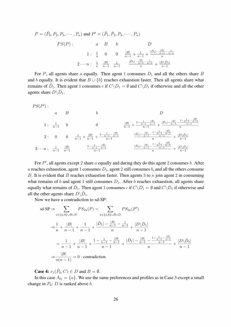
P = (P0, P2, P3, · · · , Pn) and P ′ = (P1, P2, P3, · · · , Pn)

PS(P ) : a B b D

1 : 1n

0 0 |B|n−1

+ 1n−1

+|D1|− |B|n−1

− 1n−1

n

2 · · ·n : 1n

|B|n−1

1n−1

|D1|− |B|n−1− 1n−1

n+ |D\D1|

n−1

For P , all agents share a equally. Then agent 1 consumes D1 and all the others share Band b equally. It is evident that B ∪ {b} reaches exhaustion faster. Then all agents share whatremains of D1. Then agent 1 consumes c if C\D1 = ∅ and C\D1 if otherwise and all the otheragents share D\D1.

PS(P ′) :

a B b D

1 : 1n−1 0 0 |B|

n−1 +1− 1

n−1− |B|n−1

n−1 +|D1|− |B|n−1

−1− 1

n−1−|B|n−1

n−1

n

2 : 0 0 1n−1 + |B|

n−1 +1− 1

n−1− |B|n−1

n−1

|D1|− |B|n−1−

1− 1n−1−

|B|n−1

n−1

n + |D\D1|n−1

3 · · ·n : 1n−1

|B|n−1

1− 1n−1− |B|n−1

n−1

|D1|− |B|n−1−

1− 1n−1−

|B|n−1

n−1

n + |D\D1|n−1

For P ′, all agents except 2 share a equally and during they do this agent 2 consumes b. Aftera reaches exhaustion, agent 1 consumesD1, agent 2 still consumes b, and all the others consumeB. It is evident that B reaches exhaustion faster. Then agents 3 to n join agent 2 in consumingwhat remains of b and agent 1 still consumes D1. After b reaches exhaustion, all agents shareequally what remains of D1. Then agent 1 consumes c if C\D1 = ∅ and C\D1 if otherwise andall the other agents share D\D1.

Now we have a contradiction to sd-SP:

sd-SP⇒∑

x∈{a,b}∪B∪D

PS2x(P ) =∑

x∈{a,b}∪B∪D

PS2x(P ′)

⇒ 1

n+|B|n− 1

+1

n− 1+|D1| − |B|

n−1 −1

n−1

n+|D\D1|n− 1

=1

n− 1+|B|n− 1

+1− 1

n−1 −|B|n−1

n− 1+|D1| − |B|

n−1 −1− 1

n−1− |B|n−1

n−1

n+|D\D1|n− 1

⇒ |B|n(n− 1)

= 0 : contradiction.

Case 4: r1(P0, C) ∈ D and B = ∅.In this caseAt1 = {a}. We use the same preferences and profiles as in Case 3 except a small

change in P0: D is ranked above b.

26

P0 : · · · · · · �

A(t−1)∗︷ ︸︸ ︷a � D1 � C\D1︸ ︷︷ ︸

⊂At1

� c � · · ·︸ ︷︷ ︸⊂At2

� b � · · ·︸ ︷︷ ︸⊂At1

� · · · · · · � · · · · · ·

P0 : · · · · · · �=At1︷︸︸︷a �

=At2︷ ︸︸ ︷D1 � D\D1 � b � · · ·︸ ︷︷ ︸

=At1

� c · · · · · ·︸ ︷︷ ︸=At2

� · · · · · ·

P0 : · · · · · · �=At2︷ ︸︸ ︷

b � · · ·D · · · �=At1︷︸︸︷a � · · ·︸ ︷︷ ︸

=At1

� c · · · · · ·︸ ︷︷ ︸=At2

� · · · · · ·

P = (P0, P2, P3, · · · , Pn) and P ′ = (P1, P2, P3, · · · , Pn)

PS(P ) : a D b

1 : 1n

|D1|n

0

2 · · ·n : 1n

|D1|n

+ |D\D1|n−1

1n−1

For P , all agents share a equally. Then they share D1 equally. Then agent 1 consumes c ifC\D1 = ∅ and C\D1 if otherwise and all the others share D\D1 and then b equally.

PS(P ′) :

a D b

1 : 1n−1

|D1|n−1 0

2 : 0 0 |D1|n−1 + |D\D1|

n−2 +1− |D1|

n−1− |D\D1|

n−2

n−1

3 · · ·n : 1n−1

|D1|n−1 + |D\D1|

n−2

1− |D1|n−1− |D\D1|

n−2

n−1

For P ′, all agents other than 2 share a equally and during they do this agent 2 consumes b.After a reaches exhaustion, agents other than 2 share D1 equally and agent 2 still consumes b.It is evident that D1 reaches exhaustion faster. Then agent 1 consumes c if C\D1∅ and C\D1

if otherwise, agent 3 to n share D\D1 equally, and agent 2 still consumes b. It is evident thatD\D1 reaches exhaustion faster. Then agents 3 to n join agent 2 in consuming b so they shareequally what remains of b.

Now we have a contradiction to sd-SP:

sd-SP⇒∑

x∈{a,b}∪D

PS2x(P ) =∑

x∈{a,b}∪D

PS2x(P ′)

⇒ 1

n+|D1|n

+|D\D1|n− 1

+1

n− 1

=|D1|n− 1

+|D\D1|n− 2

+1− |D1|

n−1 −|D\D1|n−2

n− 1

⇒(n− 1)2 + |D1|n(n− 1)2

= 0 : contradiction.

27

References

ABDULKADIROGLU, A. AND T. SONMEZ (1998): “Random serial dictatorship and the corefrom random endowments in house allocation problems,” Econometrica, 689–701.

——— (2003): “Ordinal efficiency and dominated sets of assignments,” Journal of EconomicTheory, 112, 157–172.

ABELLO, J. M. (1981): Toward a maximum consistent set, University of California, Depart-ment of Computer Science, College of Engineering.

BLACK, D. (1948): “On the rationale of group decision-making,” The Journal of PoliticalEconomy, 23–34.

BLACK, D., R. A. NEWING, I. MCLEAN, A. MCMILLAN, AND B. L. MONROE (1958): Thetheory of committees and elections, Springer.

BOGOMOLNAIA, A. AND H. MOULIN (2001): “A new solution to the random assignmentproblem,” Journal of Economic Theory, 100, 295–328.

BRANDL, F., F. BRANDT, AND H. G. SEEDIG (2016): “Consistent probabilistic social choice,”Econometrica, 84, 1839–1880.

CARROLL, G. (2012): “When are local incentive constraints sufficient?” Econometrica, 80,661–686.

CHANG, H.-I. AND Y. CHUN (2017): “Probabilistic assignment of indivisible objects whenagents have the same preferences except the ordinal ranking of one object,” MathematicalSocial Sciences, 90, 80–92.

CHO, W. J. (2016a): “Incentive properties for ordinal mechanisms,” Games and EconomicBehavior, 95, 168–177.

——— (2016b): “When is the probabilistic serial assignment uniquely efficient and envy-free?”Journal of Mathematical Economics, 66, 14–25.

DANILOV, V. I. AND G. A. KOSHEVOY (2013): “Maximal Condorcet Domains,” Order, 30,181–194.

FISHBURN, P. (1997): “Acyclic sets of linear orders,” Social choice and Welfare, 14, 113–124.

FISHBURN, P. C. (1984): “Probabilistic social choice based on simple voting comparisons,”The Review of Economic Studies, 51, 683–692.

——— (2002): “Acyclic sets of linear orders: A progress report,” Social Choice and Welfare,19, 431–447.

GALE, D. AND L. S. SHAPLEY (1962): “College admissions and the stability of marriage,”American Mathematical Monthly, 9–15.

28

HYLLAND, A. AND R. ZECKHAUSER (1979): “The efficient allocation of individuals to posi-tions,” Journal of Political Economy, 293–314.

KASAJIMA, Y. (2013): “Probabilistic assignment of indivisible goods with single-peaked pref-erences,” Social Choice and Welfare, 41, 203–215.

KESTEN, O. (2009): “Why do popular mechanisms lack efficiency in random environments?”Journal of Economic Theory, 144, 2209–2226.

KOJIMA, F. AND M. MANEA (2010): “Incentives in the probabilistic serial mechanism,” Jour-nal of Economic Theory, 145, 106–123.

LIU, P. AND H. ZENG (2018): “Random Assignments on Preference Domains with a TierStructure,” Mimeo.

MANDLER, M., P. MANZINI, AND M. MARIOTTI (2012): “A million answers to twenty ques-tions: Choosing by checklist,” Journal of Economic Theory, 147, 71–92.

MANEA, M. (2008): “Random serial dictatorship and ordinally efficient contracts,” Interna-tional Journal of Game Theory, 36, 489–496.

——— (2009): “Asymptotic ordinal inefficiency of random serial dictatorship,” TheoreticalEconomics, 4, 165–197.

MONJARDET, B. (2009): “Acyclic domains of linear orders: a survey,” in The Mathematics ofPreference, Choice and Order, Springer, 139–160.

MOULIN, H. (1980): “On strategy-proofness and single peakedness,” Public Choice, 35, 437–455.

ROSSIN, D. AND M. BOUVEL (2006): “The longest common pattern problem for two permu-tations,” Pure Mathematics and Applications, 17, 55–69.

SATO, S. (2013): “A sufficient condition for the equivalence of strategy-proofness and nonma-nipulability by preferences adjacent to the sincere one,” Journal of Economic Theory, 148,259–278.

SHAPLEY, L. AND H. SCARF (1974): “On cores and indivisibility,” Journal of MathematicalEconomics, 1, 23–37.

29